Ten Fast Transfer Learning Models for Carotid Ultrasound ...

diagnostics

Article

Ten Fast Transfer Learning Models for Carotid UltrasoundPlaque Tissue Characterization in Augmentation FrameworkEmbedded with Heatmaps for Stroke Risk Stratification

Skandha S. Sanagala 1,2 , Andrew Nicolaides 3 , Suneet K. Gupta 2, Vijaya K. Koppula 1 , Luca Saba 4,Sushant Agarwal 5 , Amer M. Johri 6, Manudeep S. Kalra 7 and Jasjit S. Suri 8,*

��

Citation: Sanagala, S.S.; Nicolaides,

A.; Gupta, S.K.; Koppula, V.K.; Saba,

L.; Agarwal, S.; Johri, A.M.; Kalra,

M.S.; Suri, J.S. Ten Fast Transfer

Learning Models for Carotid

Ultrasound Plaque Tissue

Characterization in Augmentation

Framework Embedded with

Heatmaps for Stroke Risk

Stratification. Diagnostics 2021, 11,

2109. https://doi.org/10.3390/

diagnostics11112109

Academic Editor: Kristoffer

Lindskov Hansen

Received: 25 October 2021

Accepted: 9 November 2021

Published: 15 November 2021

Publisher’s Note: MDPI stays neutral

with regard to jurisdictional claims in

published maps and institutional affil-

iations.

Copyright: © 2021 by the authors.

Licensee MDPI, Basel, Switzerland.

This article is an open access article

distributed under the terms and

conditions of the Creative Commons

Attribution (CC BY) license (https://

creativecommons.org/licenses/by/

4.0/).

1 CSE Department, CMR College of Engineering & Technology, Hyderabad 501401, TS, India;[email protected] (S.S.S.); [email protected] (V.K.K.)

2 CSE Department, Bennett University, Greater Noida 203206, UP, India; [email protected] Vascular Screening and Diagnostic Centre, University of Nicosia, Nicosia 1700, Cyprus;

[email protected] Department of Radiology, Azienda Ospedaliero Universitaria (A.O.U.), 10015 Cagliari, Italy;

[email protected] Global Biomedical Technologies, Roseville, CA 95661, USA; [email protected] Division of Cardiology, Queen’s University, Kingston, ON K7L 3N6, Canada; [email protected] Department of Radiology, Massachusetts General Hospital, 55 Fruit Street, Boston, MA 02114, USA;

[email protected] Stroke Diagnostic and Monitoring Division, AtheroPoint™ LLC, Roseville, CA 95661, USA* Correspondence: [email protected]; Tel.: +1-916-749-5628

Abstract: Background and Purpose: Only 1–2% of the internal carotid artery asymptomatic plaquesare unstable as a result of >80% stenosis. Thus, unnecessary efforts can be saved if these plaquescan be characterized and classified into symptomatic and asymptomatic using non-invasive B-modeultrasound. Earlier plaque tissue characterization (PTC) methods were machine learning (ML)-based,which used hand-crafted features that yielded lower accuracy and unreliability. The proposed studyshows the role of transfer learning (TL)-based deep learning models for PTC. Methods: As pertainedweights were used in the supercomputer framework, we hypothesize that transfer learning (TL)provides improved performance compared with deep learning. We applied 11 kinds of artificialintelligence (AI) models, 10 of them were augmented and optimized using TL approaches—a class ofAtheromatic™ 2.0 TL (AtheroPoint™, Roseville, CA, USA) that consisted of (i–ii) Visual GeometricGroup-16, 19 (VGG16, 19); (iii) Inception V3 (IV3); (iv–v) DenseNet121, 169; (vi) XceptionNet;(vii) ResNet50; (viii) MobileNet; (ix) AlexNet; (x) SqueezeNet; and one DL-based (xi) SuriNet-derived from UNet. We benchmark 11 AI models against our earlier deep convolutional neuralnetwork (DCNN) model. Results: The best performing TL was MobileNet, with accuracy andarea-under-the-curve (AUC) pairs of 96.10 ± 3% and 0.961 (p < 0.0001), respectively. In DL, DCNNwas comparable to SuriNet, with an accuracy of 95.66% and 92.7 ± 5.66%, and an AUC of 0.956(p < 0.0001) and 0.927 (p < 0.0001), respectively. We validated the performance of the AI architectureswith established biomarkers such as greyscale median (GSM), fractal dimension (FD), higher-orderspectra (HOS), and visual heatmaps. We benchmarked against previously developed Atheromatic™1.0 ML and showed an improvement of 12.9%. Conclusions: TL is a powerful AI tool for PTC intosymptomatic and asymptomatic plaques.

Keywords: stroke; carotid plaque characterization; symptomatic vs. asymptomatic; artificial intelli-gence; transfer learning; heatmaps

1. Introduction

Stroke is the third leading cause of mortality in the United States of America (USA) [1].According to World Health Organization (WHO) statistics, cardiovascular disease (CVD)

Diagnostics 2021, 11, 2109. https://doi.org/10.3390/diagnostics11112109 https://www.mdpi.com/journal/diagnostics

https://www.mdpi.com/journal/diagnostics

https://www.mdpi.com

https://orcid.org/0000-0003-3535-5613

https://orcid.org/0000-0003-3912-7394

https://orcid.org/0000-0002-4708-9538

https://orcid.org/0000-0003-2360-3886

https://doi.org/10.3390/diagnostics11112109


https://creativecommons.org/

https://creativecommons.org/licenses/by/4.0/

https://creativecommons.org/licenses/by/4.0/


https://www.mdpi.com/journal/diagnostics

https://www.mdpi.com/article/10.3390/diagnostics11112109?type=check_update&version=1

Diagnostics 2021, 11, 2109 2 of 31

causes 17.9 million deaths each year [2]. Atherosclerosis disease is the fundamental causeof CVD, which leads to the formation of complex plaques in the arterial walls owing to asedentary lifestyle over time [3].

Atherosclerotic plaques, particularly in the internal carotid artery (ICA), may ruptureand embolize the brain, leading to stroke. However, only a minority of plaques are unstableand rupture, producing an annual stroke rate of 1–2% in asymptomatic patients with>80% stenosis [4]. Thus, operating on all patients with >80% stenosis will result in manyunnecessary operations. In addition, the operation is associated with a 3% preoperativestroke rate. Some plaques are unstable owing to a large lipid core, a thin fibrous cap, and alow collagen content (vulnerable). Therefore, they are more likely to rupture by producingsymptoms (symptomatic or hyperechoic or unstable plaque). Compared with the morestable ones, they have a smaller lipid core, a thick fibrous cap, and a large amount ofcollagen, which tend not to produce symptoms (asymptomatic or hypoechoic or stableplaque) [5]. Therefore, it is important to characterize the plaque early, especially whenit is becoming symptomatic or likely to be unstable, leading to rupture with subsequentstroke [6,7].

Several imaging modalities exist to image the plaque, such as magnetic resonanceimaging (MRI) [8], computed tomography (CT) [9], and ultrasound (US) [10]. Ultrasoundoffers essential advantages because it is non-invasive, radiation-free, and portable proper-ties [11,12]. In addition, features like compound and harmonic imaging are now availableon standard ultrasonic equipment, yielding a resolution of 0.2 mm [12]. However, visualclassification of plaques into stable or unstable using ultrasound images is challengingowing to the inter-variability in plaque tissues [13].

Machine learning is a class of artificial intelligence (AI) that has been previously usedfor ultrasound-based tissue classification in several organs such as the liver [14,15], thy-roid [16–18], prostate [19,20], ovary [21], skin cancer [22–25], diabetes [26,27], coronary [28],and carotid atherosclerotic plaque [22,29–32]. All these methods use a trial-and-errorapproach for feature extraction, thus these methods are ad hoc and provide variableresults [33]. Therefore, there is a clear need to design and develop automated featureextraction approaches to characterize carotid atherosclerotic plaque into symptomatic andasymptomatic types.

Deep learning (DL) is a subset of AI that has revolutionized image classificationmethods [34–36]. Among all the different DL techniques available, transfer learning (TL)solves the high-performance computational challenges required for images rich withdata [37–39]. In addition to the computational problem, TL reduces the time taken fortraining the model compared with DL [40]. This saving of time can be crucial for peoplewith a high risk of stroke [41].

Several popular models exist in TL, and each model offers its own merits and de-merits. For example, some models are focused on fast optimization, while some aim forhyperparameter reduction. Some others apply the TL paradigm in edge devices, suchas NVIDIA Jetson (www.nvidia.com accessed 20 October 2021) or Raspberry Pi (fromRasberry Pi Foundation, UK) [42]. Few applications of TL have been developed in medicalimaging such as classification of Wilson disease [43], COVID pneumonia [44–47], braintumour [37], and so on, which has shown superior performance over DL. In this study,we choose ten types of TL architectures, where each one of these carries advantages suchas (a) intense neural network, (b) modified kernel sizes, (c) solving vanishing gradientproblems, and (d) feed-forward nature to the features [48]. Therefore, we hypothesize thatthe performance of TL is superior or comparable to that of DL.

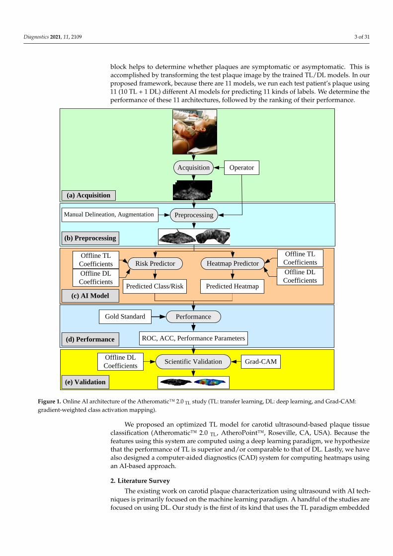
The architecture of the proposed global AI model is shown in Figure 1. It containsfive blocks: (i) image acquisition, (ii) pre-processing, (iii) AI-based models, and (iv–v) per-formance evaluation and validation. The image acquisition block is used for scanningthe internal carotid artery. These scans are normalized and manually delineated in thepre-processing block to obtain the plaque region-of-interest (ROI). As the cohort size wassmall, we added the augmentation block as part of the pre-processing step. The AI model

www.nvidia.com

Diagnostics 2021, 11, 2109 3 of 31

block helps to determine whether plaques are symptomatic or asymptomatic. This isaccomplished by transforming the test plaque image by the trained TL/DL models. In ourproposed framework, because there are 11 models, we run each test patient’s plaque using11 (10 TL + 1 DL) different AI models for predicting 11 kinds of labels. We determine theperformance of these 11 architectures, followed by the ranking of their performance.

Diagnostics 2021, 11, x FOR PEER REVIEW 3 of 32

internal carotid artery. These scans are normalized and manually delineated in the pre-

processing block to obtain the plaque region-of-interest (ROI). As the cohort size was

small, we added the augmentation block as part of the pre-processing step. The AI model

block helps to determine whether plaques are symptomatic or asymptomatic. This is ac-

complished by transforming the test plaque image by the trained TL/DL models. In our

proposed framework, because there are 11 models, we run each test patient’s plaque using

11 (10 TL + 1 DL) different AI models for predicting 11 kinds of labels. We determine the

performance of these 11 architectures, followed by the ranking of their performance.

We proposed an optimized TL model for carotid ultrasound-based plaque tissue clas-

sification (Atheromatic™ 2.0 TL, AtheroPoint™, Roseville, CA, USA). Because the features

using this system are computed using a deep learning paradigm, we hypothesize that the

performance of TL is superior and/or comparable to that of DL. Lastly, we have also de-

signed a computer-aided diagnostics (CAD) system for computing heatmaps using an AI-

based approach.

Acquisition Operator

PreprocessingManual Delineation, Augmentation

(a) Acquisition

(b) Preprocessing

Risk Predictor

Offline TL

Coefficients

Offline DL

Coefficients

(c) AI Model

Predicted Class/Risk

Performance

ROC, ACC, Performance Parameters(d) Performance

(e) Validation

Grad-CAM

Gold Standard

Scientific ValidationOffline DL

Coefficients

Heatmap Predictor

Predicted Heatmap

Offline TL

Coefficients

Offline DL

Coefficients

Figure 1. Online AI architecture of the Atheromatic™ 2.0 TL study (TL: transfer learning, DL: deep learning, and Grad-

CAM: gradient-weighted class activation mapping).

Figure 1. Online AI architecture of the Atheromatic™ 2.0 TL study (TL: transfer learning, DL: deep learning, and Grad-CAM:gradient-weighted class activation mapping).

We proposed an optimized TL model for carotid ultrasound-based plaque tissueclassification (Atheromatic™ 2.0 TL, AtheroPoint™, Roseville, CA, USA). Because thefeatures using this system are computed using a deep learning paradigm, we hypothesizethat the performance of TL is superior and/or comparable to that of DL. Lastly, we havealso designed a computer-aided diagnostics (CAD) system for computing heatmaps usingan AI-based approach.

2. Literature Survey

The existing work on carotid plaque characterization using ultrasound with AI tech-niques is primarily focused on the machine learning paradigm. A handful of the studies arefocused on using DL. Our study is the first of its kind that uses the TL paradigm embedded

Diagnostics 2021, 11, 2109 4 of 31

with heatmaps for PTC. The section briefly presents the works on PTC. Detailed tabulationis described in the discussion section.

Seabra et al. [49] used graph cut techniques for the characterization of 3D ultrasound.It allows for the detection and quantification of the vulnerable plaque. The same set ofauthors in [50] estimated the volume inside the ROI plaque using the Bayesian technique.They compared the proposed method with a gold standard and achieved better resultswith greyscale median (GSM) < 32. In [51], they characterized the plaque components suchas lipids, fibrotic, and calcified using the Rayleigh mixture model (RMM).

Afonso et al. [52] proposed a CAD tool (AtheroRisk™, AtheroPoint, Roseville, CA,USA) to characterize the plaque echogenicity using an activity index and enhanced activityindex (EAI). The authors achieved an area-under-the-curve (AUC) of 64.96%, 73.29%, and90.57% for the degree of stenosis, activity index, and enhanced activity index, respectively.This AtheroRisk™ CAD system was able to measure the plaque rupture risk. Loizou et al.identified and segmented the carotid plaque in M-mode ultrasound videos (MUVs) using asnake algorithm [53–55]. In [56], the authors studied the variations in texture features suchas spatial gray level dependence matrices (SGLD) and gray level difference statistic (GLDS)in the MUV framework to classify them using a support vector machine (SVM) classifier.Doonan et al. [57] studied the relationship between textural and echo density featuresof carotid plaque by applying the principal component analysis (PCA)-based featureselection technique. The authors showed a moderate coefficient of correlation (r) betweenthese two features, which range from 0.211 to 0.641. In addition to the above studies,Acharya et al. [58–60], Gastounioti et. al. [61], Skandha et. al. [62], and Saba et. al. [63] alsoconducted studies in the area of PTC using AI methods. This will be discussed in detail inSection 5, labeled benchmarking.

3. Methodology

This section focuses on patient demographics, ultrasound acquisition, pre-processing,and augmentation protocol. We also described all 11 AI architectures, consisting of tentransfer learning architectures and one deep learning architecture labelled as SuriNet.These are then benchmarked against the deep convolution neural network (DCNN).

3.1. Patient Demographics

This cohort consisted of 346 patients with a mean age of 69.9 ± 7.8 and 61% malepatients having an internal carotid artery (ICA) stenosis of 50% to 99%. The study wasapproved by the ethical committee of St. Mary’s Hospital, Imperial College, London, UK(in 2000). The cohort consisted of 196 symptomatic and 150 asymptomatic patients. All thesymptomatic patients have ipsilateral cerebral hemispheric symptoms (amaurosis fugax)(AF), transient ischemic attacks, and previous history of stroke. Overall, the symptomaticclass contained 38 AF, 70 transient ischaemic attack (TIAs), and 88 strokes, totaling 196. Allthe asymptomatic patients showed no abnormalities during the neurological study. Thesame cohort was used in our previous studies [29,32,40,58,62–65].

3.2. Ultrasound Data Acquisition and Pre-Processing

All the US scans were acquired using an ATL machine (Model: HDI 3000; Make:Advanced Technology Laboratories, Seattle, WA, USA) in Irvine Laboratory for Cardio-vascular Investigation and Research, St. Mary’s Hospital, UK. This scanner was equippedwith a linear broadband width 4–7 MHz (multifrequency) transducer with a 20 pixel/mmresolution. We used proprietary software called “PTAS” developed by Icon soft Interna-tional Ltd., Greenford, London, UK for normalization and plaque ROI delineation, as usedin previous studies [29,32,58,62,64,65]. The medical practitioners delineated the plaqueregion-of-interest (ROI) using the mouse and trackball; these were then saved in a separatefile. Full scans and delineated plaques are shown in Figure 2.

Diagnostics 2021, 11, 2109 5 of 31


in previous studies [29,32,58,62,64,65]. The medical practitioners delineated the plaque

region-of-interest (ROI) using the mouse and trackball; these were then saved in a separate

file. Full scans and delineated plaques are shown in Figure 2.

Figure 2. (a) Top: symptomatic (row 1 and row 3) and (b) down: asymptomatic; (row 5 and row 7): original carotid full

scans; row 2, row 4, row 6, and row 8 are the plaque delineated cut sections of (a) symptomatic and (b) asymptomatic

plaques after pre-processing and delineation.

3.3. Augmentation

Our cohort was unbalanced, consisting of 196 symptomatic and 150 asymptomatic.

Therefore, we choose to balance using the augmentation strategy prior to offline training

and online predicting processes. We accomplished this by adding 4 symptomatic and 50

asymptomatic augmented images using random linear transformations such as flipping,

rotation by 90 degrees, rotation by 270 degrees, and skew operations. This resulted in a

balanced cohort, containing 200 images in each class. Further, the database was incre-

mented two to six times, consisting of an equal number of images using linear transfor-

mations. This resulted in six folds of the augmented cohort. We represent these folds as

Augmented 2× (Aug 2×), Augmented 3× (Aug 3×), Augmented 4× (Aug 4×), Augmented

5× (Aug 5×), and Augmented 6× (Aug 6×). Thus, every fold contained 200 × n images in

each class, where n is the augmented fold.

3.4. Transfer Learning

The choice of the TL architecture for PTC was motivated by (a) the diversity of the

TL models and (b) the depth of the neural network models. Thus, we took two architec-

tures from the VGG group (VGG-16 and 19), two architectures from the DenseNet archi-

tectures (DenseNet121 and 169), and two architectures from the ResNet architectures (Res-

Net50 and 101). All these models had a depth of neural networks extending to 169 layers

while ensuring diversity. Note that some of the architectures such as MobileNet and Xcep-

tionNet are the most current, state-of-the-art, and popular TL architectures, demonstrat-

ing faster optimization (see Figure 3).

Figure 2. (a) Top: symptomatic (row 1 and row 3) and (b) down: asymptomatic; (row 5 and row 7): original carotid fullscans; row 2, row 4, row 6, and row 8 are the plaque delineated cut sections of (a) symptomatic and (b) asymptomaticplaques after pre-processing and delineation.

3.3. Augmentation

Our cohort was unbalanced, consisting of 196 symptomatic and 150 asymptomatic.Therefore, we choose to balance using the augmentation strategy prior to offline trainingand online predicting processes. We accomplished this by adding 4 symptomatic and50 asymptomatic augmented images using random linear transformations such as flipping,rotation by 90 degrees, rotation by 270 degrees, and skew operations. This resulted in abalanced cohort, containing 200 images in each class. Further, the database was incrementedtwo to six times, consisting of an equal number of images using linear transformations. Thisresulted in six folds of the augmented cohort. We represent these folds as Augmented 2×(Aug 2×), Augmented 3× (Aug 3×), Augmented 4× (Aug 4×), Augmented 5× (Aug 5×),and Augmented 6× (Aug 6×). Thus, every fold contained 200 × n images in each class,where n is the augmented fold.

3.4. Transfer Learning

The choice of the TL architecture for PTC was motivated by (a) the diversity of the TLmodels and (b) the depth of the neural network models. Thus, we took two architecturesfrom the VGG group (VGG-16 and 19), two architectures from the DenseNet architectures(DenseNet121 and 169), and two architectures from the ResNet architectures (ResNet50and 101). All these models had a depth of neural networks extending to 169 layers whileensuring diversity. Note that some of the architectures such as MobileNet and XceptionNetare the most current, state-of-the-art, and popular TL architectures, demonstrating fasteroptimization (see Figure 3).

Diagnostics 2021, 11, 2109 6 of 31Diagnostics 2021, 11, x FOR PEER REVIEW 6 of 32

Natural Images (ImageNet) Color Image (CIFAR)

Pretrained Transfer Weights

Offline System

Pretrained Models

Model Retraining

AlexNet

XceptionNet

MobileNet

Inception V3

VGG 16, 19

DenseNet 169

DenseNet121

ResNet50

SqueezeNet

TL Models

FCN

Transfer Weights

Fine Tune Models

FT Networks

CUS (tr)

GT (tr).

Prediction System

CUS (tr)

GT (tr).

CUS (te)

GT (te)

Predicted Labels

Performance

Predicted LablesOnline System

Figure 3. Global TL architecture using 10 different TL models (i–ii) Visual Geometric Group-16, 19 (VGG16, 19); (iii) In-

ception V3 (IV3); (iv–v) DenseNet121, 169; (vi) XceptionNet; (vii) ResNet50; (viii) MobileNet; (ix) AlexNet; and (x)

SqueezeNet. Te stands for testing and tr stands for training. FN: fine-tune networks.

3.4.1. VGG-16 and VGG-19

Visual Geometry Group (VGG-16) is a popular pre-trained model developed by Si-

monyan et al. [66] to increase the neural networks’ depth by adding a number of 3 × 3

convolution filters. The purpose of VGGx is to design a very deep CNN for complex pat-

tern understanding in the input features, typically adapted for object recognition in med-

ical imaging and computer vision. The architecture of the VGG-16 and 19 is shown in

Figure 4, where the input block accepts the image of size 224 × 224. VGG-19 is three layers

Figure 3. Global TL architecture using 10 different TL models (i–ii) Visual Geometric Group-16, 19 (VGG16, 19); (iii) Incep-tion V3 (IV3); (iv–v) DenseNet121, 169; (vi) XceptionNet; (vii) ResNet50; (viii) MobileNet; (ix) AlexNet; and (x) SqueezeNet.Te stands for testing and tr stands for training. FN: fine-tune networks.

3.4.1. VGG-16 and VGG-19

Visual Geometry Group (VGG-16) is a popular pre-trained model developed bySimonyan et al. [66] to increase the neural networks’ depth by adding a number of3 × 3 convolution filters. The purpose of VGGx is to design a very deep CNN for complexpattern understanding in the input features, typically adapted for object recognition inmedical imaging and computer vision. The architecture of the VGG-16 and 19 is shown inFigure 4, where the input block accepts the image of size 224 × 224. VGG-19 is three layers

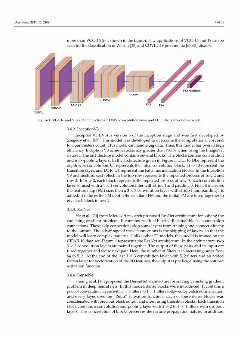
Diagnostics 2021, 11, 2109 7 of 31

more than VGG-16 (not shown in the figure). Few applications of VGG-16 and 19 can beseen for the classification of Wilson [38] and COVID-19 pneumonia [67,68] disease.


more than VGG-16 (not shown in the figure). Few applications of VGG-16 and 19 can be

seen for the classification of Wilson [38] and COVID-19 pneumonia [67,68] disease.

CONV1

CONV2

CONV3

CONV4

CONV4

FC6 FC7

FC8+Softmax

Figure 4. VGG16 and VGG19 architectures; CONV: convolution layer and FC: fully connected network.

3.4.2. InceptionV3

InceptionV3 (IV3) is version 3 of the inception stage and was first developed by Sze-

gedy et al. [69]. This model was developed to overcome the computational cost and low

parameters count. This model can handle big data. Thus, this model has overall high effi-

ciency. Inception V3 achieves accuracy greater than 78.1% when using the ImageNet da-

taset. The architecture model contains several blocks. The blocks contain convolution and

max-pooling layers. In the architecture given in Figure 5, DL1 to DL6 represent the depth

wise convolution, C1 represents the initial convolution block, T1 to T3 represent the tran-

sition layer, and D1 to D4 represent the batch normalization blocks. In the Inception V3

architecture, each block in the top row represents the repeated process of row 2 and row

3. In row 2, each block represents the repeated process of row 3. Each convolution layer is

fused with a 1 × 1 convolution filter with stride 1 and padding 0. First, it increases the

feature map (FM) size, then a 3 × 3 convolution layer with stride 1 and padding 1 is added.

It reduces the FM depth; the resultant FM and the initial FM are fused together to give

each block in row 2.

Figure 4. VGG16 and VGG19 architectures; CONV: convolution layer and FC: fully connected network.

3.4.2. InceptionV3

InceptionV3 (IV3) is version 3 of the inception stage and was first developed bySzegedy et al. [69]. This model was developed to overcome the computational cost andlow parameters count. This model can handle big data. Thus, this model has overall highefficiency. Inception V3 achieves accuracy greater than 78.1% when using the ImageNetdataset. The architecture model contains several blocks. The blocks contain convolutionand max-pooling layers. In the architecture given in Figure 5, DL1 to DL6 represent thedepth wise convolution, C1 represents the initial convolution block, T1 to T3 represent thetransition layer, and D1 to D4 represent the batch normalization blocks. In the InceptionV3 architecture, each block in the top row represents the repeated process of row 2 androw 3. In row 2, each block represents the repeated process of row 3. Each convolutionlayer is fused with a 1 × 1 convolution filter with stride 1 and padding 0. First, it increasesthe feature map (FM) size, then a 3 × 3 convolution layer with stride 1 and padding 1 isadded. It reduces the FM depth; the resultant FM and the initial FM are fused together togive each block in row 2.

3.4.3. ResNet

He et al. [70] from Microsoft research proposed ResNet architecture for solving thevanishing gradient problem. It contains residual blocks. Residual blocks contain skipconnections. These skip connections skip some layers from training and connect directlyto the output. The advantage of these connections is the skipping of layers, so that themodel will learn complex patterns. Unlike other TL models, this model is trained on theCIFAR-10 data set. Figure 6 represents the ResNet architecture. In the architecture, two3 × 3 convolution layers are paired together. The output of these pairs and its input arefused together and fed to next pair. Here, the number of filters is in increasing order from64 to 512. At the end of the last 3 × 3 convolution layer with 512 filters and an addedflatten layer for vectorization of the 2D features, the output is predicted using the softmaxactivation function.

3.4.4. DenseNet

Huang et al. [48] proposed the DenseNet architecture for solving vanishing gradientproblem in deep neural nets. In this model, dense blocks were introduced. It contains apool of convolution layers with 3 × 3 filters to 1 × 1 filters followed by batch normalization,and every layer uses the “ReLu” activation function. Each of these dense blocks wasconcatenated with previous block output and input using transition blocks. Each transitionblock contains a convolution and pooling layer with 2 × 2 to 1 × 1 filters with dropoutlayers. This concertation of blocks preserves the feature propagation nature. In addition,

Diagnostics 2021, 11, 2109 8 of 31

the author proposed architectures (DenseNet-121, 169, 201, and 264) to increase the denseblock. Figure 7 shows the DenseNet architecture.


Figure 5. Inception V3 architecture.

3.4.3. ResNet

He et al. [70] from Microsoft research proposed ResNet architecture for solving the

vanishing gradient problem. It contains residual blocks. Residual blocks contain skip con-

nections. These skip connections skip some layers from training and connect directly to

the output. The advantage of these connections is the skipping of layers, so that the model

will learn complex patterns. Unlike other TL models, this model is trained on the CIFAR-

10 data set. Figure 6 represents the ResNet architecture. In the architecture, two 3 × 3 con-

volution layers are paired together. The output of these pairs and its input are fused to-

gether and fed to next pair. Here, the number of filters is in increasing order from 64 to

512. At the end of the last 3 × 3 convolution layer with 512 filters and an added flatten

layer for vectorization of the 2D features, the output is predicted using the softmax acti-

vation function.

Figure 6. ResNet Architecture.




3.4.3. ResNet

He et al. [70] from Microsoft research proposed ResNet architecture for solving the

vanishing gradient problem. It contains residual blocks. Residual blocks contain skip con-

nections. These skip connections skip some layers from training and connect directly to

the output. The advantage of these connections is the skipping of layers, so that the model

will learn complex patterns. Unlike other TL models, this model is trained on the CIFAR-

10 data set. Figure 6 represents the ResNet architecture. In the architecture, two 3 × 3 con-

volution layers are paired together. The output of these pairs and its input are fused to-

gether and fed to next pair. Here, the number of filters is in increasing order from 64 to

512. At the end of the last 3 × 3 convolution layer with 512 filters and an added flatten

layer for vectorization of the 2D features, the output is predicted using the softmax acti-

vation function.

Figure 6. ResNet Architecture. Figure 6. ResNet Architecture.

Diagnostics 2021, 11, 2109 9 of 31


3.4.4. DenseNet

Huang et al. [48] proposed the DenseNet architecture for solving vanishing gradient

problem in deep neural nets. In this model, dense blocks were introduced. It contains a

pool of convolution layers with 3 × 3 filters to 1 × 1 filters followed by batch normalization,

and every layer uses the “ReLu” activation function. Each of these dense blocks was con-

catenated with previous block output and input using transition blocks. Each transition

block contains a convolution and pooling layer with 2 × 2 to 1 × 1 filters with dropout

layers. This concertation of blocks preserves the feature propagation nature. In addition,

the author proposed architectures (DenseNet-121, 169, 201, and 264) to increase the dense

block. Figure 7 shows the DenseNet architecture.

Figure 7. DenseNet architecture with three dense blocks and three transition blocks, followed by the fully connected net-

work. Post processing is represented by softmax.

3.4.5. MobileNet

Howard et al. [42] from Google developed the MobileNet architecture. The main in-

spiration of MobileNet comes from the IV3 network. It aims to solve resource constraint

problems such as working on edge devices like NVIDIA Jetson (www.nvidia.com ac-

cessed 20 October 2021) or Rasberry Pi (from Rasberry Pi Foundation, Cambridge, UK).

This architecture is a small, low latency, and low power model. This was the first com-

puter vision model developed for TensorFlow for mobile devices. It contains 28 layers and

uses the TFlite (database) library. Figure 8 presents the architecture of MobileNet archi-

tecture. This model contains bottleneck residual blocks (BRBs), also referred to as inverted

residual blocks used for reducing the number of training parameters in the model.

Figure 7. DenseNet architecture with three dense blocks and three transition blocks, followed by the fully connectednetwork. Post processing is represented by softmax.

3.4.5. MobileNet

Howard et al. [42] from Google developed the MobileNet architecture. The maininspiration of MobileNet comes from the IV3 network. It aims to solve resource constraintproblems such as working on edge devices like NVIDIA Jetson (www.nvidia.com accessed20 October 2021) or Rasberry Pi (from Rasberry Pi Foundation, Cambridge, UK). Thisarchitecture is a small, low latency, and low power model. This was the first computervision model developed for TensorFlow for mobile devices. It contains 28 layers and usesthe TFlite (database) library. Figure 8 presents the architecture of MobileNet architecture.This model contains bottleneck residual blocks (BRBs), also referred to as inverted residualblocks used for reducing the number of training parameters in the model.


Figure 8. MobileNet Architecture, BRB: bottleneck and residual blocks.

3.4.6. XceptionNet

Chollet et al. [71] from Google proposed modifying IV3 by replacing the inception

modules with modified depth-wise separable convolution layers. This architecture con-

tains 36 layers. In comparison with IV3, XceptionNet is lightweight and contains the same

number of parameters as IV3. This architecture outperforms InceptinV3 with top-1 accu-

racy of 0.790 and top-5 accuracy of 0.945. Figure 9 represents the architecture of Xception-

Net.

Figure 9. XceptionNet architecture.


3.4.6. XceptionNet

Chollet et al. [71] from Google proposed modifying IV3 by replacing the inceptionmodules with modified depth-wise separable convolution layers. This architecture contains36 layers. In comparison with IV3, XceptionNet is lightweight and contains the samenumber of parameters as IV3. This architecture outperforms InceptinV3 with top-1 accuracyof 0.790 and top-5 accuracy of 0.945. Figure 9 represents the architecture of XceptionNet.

www.nvidia.com

Diagnostics 2021, 11, 2109 10 of 31



3.4.6. XceptionNet

Chollet et al. [71] from Google proposed modifying IV3 by replacing the inception

modules with modified depth-wise separable convolution layers. This architecture con-

tains 36 layers. In comparison with IV3, XceptionNet is lightweight and contains the same

number of parameters as IV3. This architecture outperforms InceptinV3 with top-1 accu-

racy of 0.790 and top-5 accuracy of 0.945. Figure 9 represents the architecture of Xception-

Net.



3.4.7. AlexNet

Alex Krizhevsky et al. [72] proposed AlexNet in 2012 for solving complicated Ima-geNet challenges. It is the first CNN architecture built for solving complex computer visionproblems. This architecture achieves a top-5 error rate of 15.3%. This architecture shifts theparadigm of AI entirely. It takes 256 × 256 size image input and contains five convolutionlayers followed by max-pooling with two fully connected networks. The output layer isthe softmax layer. The sample architecture is shown in Figure 10.


3.4.7. AlexNet

Alex Krizhevsky et al. [72] proposed AlexNet in 2012 for solving complicated

ImageNet challenges. It is the first CNN architecture built for solving complex computer

vision problems. This architecture achieves a top-5 error rate of 15.3%. This architecture

shifts the paradigm of AI entirely. It takes 256 × 256 size image input and contains five

convolution layers followed by max-pooling with two fully connected networks. The out-

put layer is the softmax layer. The sample architecture is shown in Figure 10.

Figure 10. AlexNet architecture.

3.4.8. SqueezeNet

Landola et al. [73] proposed a 50× times smaller model than the AlexNet architecture.

Nevertheless, the authors achieved 82.5% in top-5 accuracy on ImageNet. This model con-

tains a novel “Fire Module”. It contains a 1 × 1 filtered squeeze convolution layer fed to

the “Expand Module”, which contains a mix of 1 × 1 to 3 × 3 filters for convolution. The

squeeze layer (Fire Module) helps to reduce the number of input channels to 3 × 3. The

architecture of the SqueezeNet and Fire Module is shown in Figure 11. In this study, we

transferred trained weights to SqueezeNet initial layers and fed our cohort at the end

layer.

Figure 11. SqueezeNet architecture.


3.4.8. SqueezeNet

Landola et al. [73] proposed a 50× times smaller model than the AlexNet architecture.Nevertheless, the authors achieved 82.5% in top-5 accuracy on ImageNet. This modelcontains a novel “Fire Module”. It contains a 1 × 1 filtered squeeze convolution layer fedto the “Expand Module”, which contains a mix of 1 × 1 to 3 × 3 filters for convolution. Thesqueeze layer (Fire Module) helps to reduce the number of input channels to 3 × 3. The

Diagnostics 2021, 11, 2109 11 of 31

architecture of the SqueezeNet and Fire Module is shown in Figure 11. In this study, wetransferred trained weights to SqueezeNet initial layers and fed our cohort at the end layer.


3.4.7. AlexNet

Alex Krizhevsky et al. [72] proposed AlexNet in 2012 for solving complicated

ImageNet challenges. It is the first CNN architecture built for solving complex computer

vision problems. This architecture achieves a top-5 error rate of 15.3%. This architecture

shifts the paradigm of AI entirely. It takes 256 × 256 size image input and contains five

convolution layers followed by max-pooling with two fully connected networks. The out-

put layer is the softmax layer. The sample architecture is shown in Figure 10.


3.4.8. SqueezeNet

Landola et al. [73] proposed a 50× times smaller model than the AlexNet architecture.

Nevertheless, the authors achieved 82.5% in top-5 accuracy on ImageNet. This model con-

tains a novel “Fire Module”. It contains a 1 × 1 filtered squeeze convolution layer fed to

the “Expand Module”, which contains a mix of 1 × 1 to 3 × 3 filters for convolution. The

squeeze layer (Fire Module) helps to reduce the number of input channels to 3 × 3. The

architecture of the SqueezeNet and Fire Module is shown in Figure 11. In this study, we

transferred trained weights to SqueezeNet initial layers and fed our cohort at the end

layer.



3.5. Deep Learning Architecture: SuriNet

In our study, we benchmarked TL architectures with two DL architectures. One isconventional CNN and the other is SuriNet architecture. Although the UNet networkis very popular for segmentation in medical image analysis, we used a modified UNetarchitecture called SuriNet for classification purposes. In the proposed SuriNet architecture,we used separable convolution neural networks to reduce the overfitting and the numberof parameters required for training. Figure 12 shows the SuriNet architecture. Table 1 givesthe detailed number of training parameters for SuriNet.


3.5. Deep Learning Architecture: SuriNet

In our study, we benchmarked TL architectures with two DL architectures. One is

conventional CNN and the other is SuriNet architecture. Although the UNet network is

very popular for segmentation in medical image analysis, we used a modified UNet ar-

chitecture called SuriNet for classification purposes. In the proposed SuriNet architecture,

we used separable convolution neural networks to reduce the overfitting and the number

of parameters required for training. Figure 12 shows the SuriNet architecture. Table 1

gives the detailed number of training parameters for SuriNet.

SuriNet

Figure 12. SuriNet architecture.

Table 1. SuriNet architecture parameters.

Layer Type Shape #Param

Convolution 2D 128 × 128 × 32 896

Batch normalization 128 × 128 × 32 128

Separable Convolution 2D 128 × 128 × 64 2400


MaxPooling 2D 64 × 64 × 64 0



MaxPooling 2D 32 × 32 × 128 0

Separable Convolution 2D 32 × 32 × 256 34,176


MaxPooling 2D 16 × 16 × 256 0



MaxPooling 2D 8 × 8 × 64 0







Flatten 1024 0

Dense 1024 1,049,600

Dropout 0.5 0

Dense 512 524,800

Dropout 0.5 0

Dense (softmax) 2 1026

Figure 12. SuriNet architecture.

3.6. Experimental Protocol

Our study used 12 AI models (10 TL and 2 DL) with six augmentation folds and1000 epochs using the K10 cross-validation protocol. It totals to ~720,000 (720 K) runs forfinding the optimization point of each AI model. The mean accuracy of each model iscalculated using the following section.

Diagnostics 2021, 11, 2109 12 of 31

Table 1. SuriNet architecture parameters.

Layer Type Shape #ParamConvolution 2D 128 × 128 × 32 896




MaxPooling 2D 64 × 64 × 64 0



MaxPooling 2D 32 × 32 × 128 0



MaxPooling 2D 16 × 16 × 256 0










Flatten 1024 0

Dense 1024 1,049,600

Dropout 0.5 0

Dense 512 524,800

Dropout 0.5 0

Dense (softmax) 2 1026

Total Trainable Parameters 1,687,330

3.6.1. Accuracy Bar Charts for Each Cohort Corresponding to All AI Models

If η(m, k) represents the accuracy of an AI model “m” using cross-validation combi-nation “k” out of total combinations K, then the mean accuracy for all the combinations forthe model “m”, represented by η(m) can be mathematically given by Equation (1). Notethat we considered K10 protocol in our paradigm, so K = K10 = 10.

η(m) =1K

K

∑k=1

η(m, k) (1)

3.6.2. Performance Analysis and Visualization of SuriNet

The objective of this experiment was to evaluate the performance of SuriNet usingEquation (1). In addition, SuriNet is based on the DL model. It is end-to-end trained on the

Diagnostics 2021, 11, 2109 13 of 31

target labels. So, we can visualize the intermediate layers’ feature maps of symptomaticand asymptomatic plaques. In this regard, we considered the optimized augmentation foldout of 10 combinations as the combination with the best performance for the visualizationof the filters.

4. Results

This section discusses three sets of experimentations for comparison of TL versus DL toprove the hypothesis. The first experiment is the 3D optimization of the ten TL architecturesby varying the augmentation folds. The second experiment is the 3D optimization of theSuriNet architecture by varying the same fold. The third experiment is the benchmarkingTL architectures with SuriNet and CNN by calculating the AUC.

4.1. 3D Optimization of TL Architectures and Benchmarking against CNN

In this experiment, we used all the TL architectures for finding the optimized TL byvarying the augmentation folds. There are 10 TL architectures, 6 augmentation folds, K10cross-validation protocol, and 1000 epochs. The model is trained by empirically selecting eachmodel’s flatten point at a loss versus accuracy, thus there were 12 × 6 × 10 × 1000 ~720 K runs.We used a total of 720,000 runs to obtain the optimization point. This is a reasonably largenumber of computations and needs high computation power. Thus, we used the Nvidia DGXV100 supercomputer at Bennett University, Gr. Noida. Figure 13 shows the performance often AI architectures, and the red arrow indicates the optimization point for each AI modelwhen ran over six augmentations. The corresponding values are represented in Table 2. UsingEquation (1), we calculate the mean accuracy of the AI models.


Figure 13. 3D bar chart representation of the AI model accuracy vs. augmentation folds, light blue color bar represents the

Aug 1×, orange color bar represents the Aug 2×, gray color bar represents Aug 3×, yellow bar represents the Aug 4×, dark

blue color represents Aug 5×, green color bar represents Aug 6×, and red arrow represents the optimization point of each

classifier.

As seen in Figure 13, MobileNet and DenseNet 169 show better accuracy than other

TL architectures. They showed 96.19% and 95.64% accuracy, respectively. Aug 2× is the

optimization point for both models. Table 3 shows the comparison between ten types of

TL, which include VGG16, VGG19, DenseNet121, XceptionNet, MobileNet, AlexNet, In-

ceptionV3, and SqueezeNet, along with seven types of DL. The ten types of TL and seven

types of DL include CNN5, CNN7, CNN9, CNN11, CNN13, CNN15, and SuriNet, respec-

tively. Note that CNN5 to CNN15 were taken from our previous study [62], so we have

elaborated on the CNN architecture in Appendix A.

Table 2. Accuracies of 10 TL and 2 DL models for 6 augmentations. Bold represents the optimiza-

tion point of each classifier

AI Model Balanced Aug 2× Aug 3× Aug 4× Aug 5× Aug 6×

VGG16 48 47.5 47.97 66.72 79.12 70.87

VGG19 81.5 87.33 88.07 89.08 87.5 91.56

ResNet50 70.4 75.4 78.2 70.5 68.7 66.5

DenseNet169 80.9 95.64 86.14 86.57 85.06 85.66

DenseNet121 76.99 79.69 73.29 85.17 77.33 75.81

Xception Net 67.49 82.74 79.99 81.87 76.49 86.55

MobileNet 81.49 96.19 72.82 79.99 83.59 81.24

InceptionV3 82.18 91.24 79 84.69 83.33 86.88

SuriNet 80.32 85.09 86.50 88.93 92.77 84.95

CNN [62] 84.24 90.6 92.12 92.99 95.66 92.66

AlexNet 62.84 74.29 80.21 91.09 78.81 80.91

SqueezeNet 74.65 83.20 79.23 83.12 81.33 82.00

In the SuriNet architecture, there are 22 layers, while there is a varying number of

layers in the CNN architecture, ranging from 5 to 15. It is important to note that all CNNs

except CNN5 have accuracies above 92.27%. The overall mean and standard deviation of

the DL accuracies was 90.86 ± 3.15%. The innovation of the current study was the design

and development of TLs. They are benchmarking against DL. In Table 3, the mean and standard deviation of ten TLs was 89.35 ± 2.54%. Thus, the mean accuracy of TL systems

Figure 13. 3D bar chart representation of the AI model accuracy vs. augmentation folds, light blue color bar representsthe Aug 1×, orange color bar represents the Aug 2×, gray color bar represents Aug 3×, yellow bar represents the Aug 4×,dark blue color represents Aug 5×, green color bar represents Aug 6×, and red arrow represents the optimization point ofeach classifier.

As seen in Figure 13, MobileNet and DenseNet 169 show better accuracy than otherTL architectures. They showed 96.19% and 95.64% accuracy, respectively. Aug 2× is theoptimization point for both models. Table 3 shows the comparison between ten typesof TL, which include VGG16, VGG19, DenseNet121, XceptionNet, MobileNet, AlexNet,InceptionV3, and SqueezeNet, along with seven types of DL. The ten types of TL andseven types of DL include CNN5, CNN7, CNN9, CNN11, CNN13, CNN15, and SuriNet,respectively. Note that CNN5 to CNN15 were taken from our previous study [62], so wehave elaborated on the CNN architecture in Appendix A.

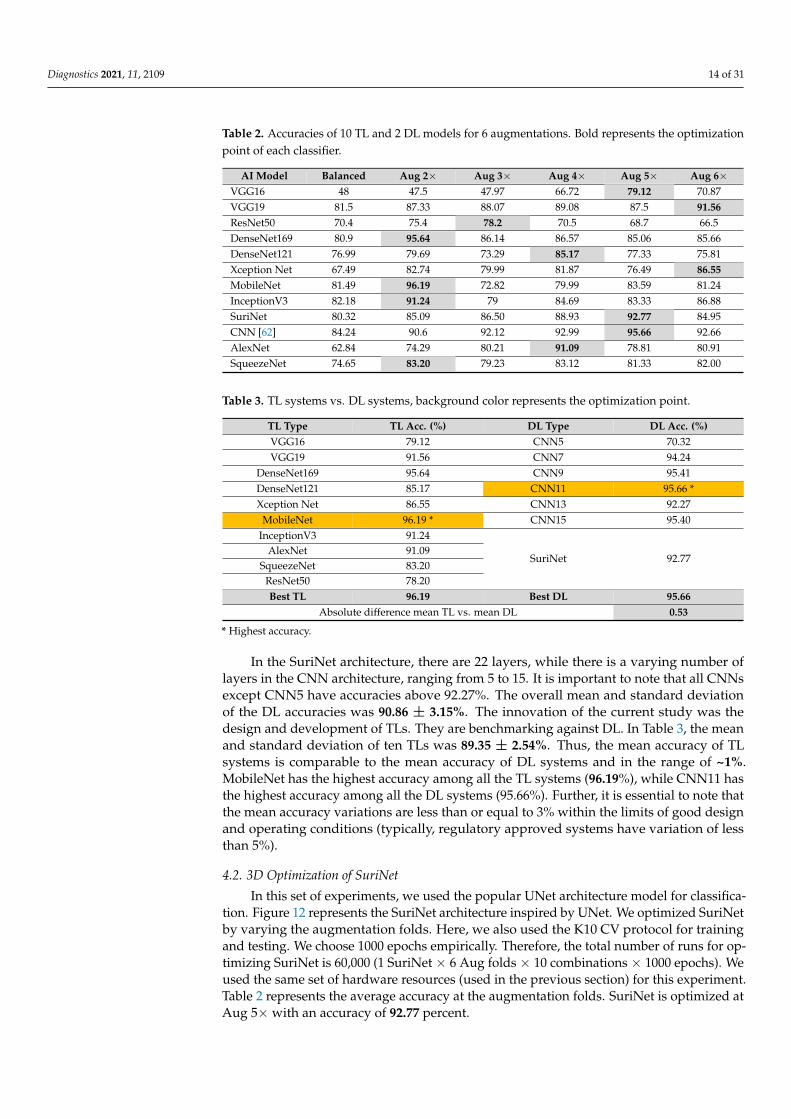
Diagnostics 2021, 11, 2109 14 of 31

Table 2. Accuracies of 10 TL and 2 DL models for 6 augmentations. Bold represents the optimizationpoint of each classifier.

AI Model Balanced Aug 2× Aug 3× Aug 4× Aug 5× Aug 6×VGG16 48 47.5 47.97 66.72 79.12 70.87VGG19 81.5 87.33 88.07 89.08 87.5 91.56ResNet50 70.4 75.4 78.2 70.5 68.7 66.5DenseNet169 80.9 95.64 86.14 86.57 85.06 85.66DenseNet121 76.99 79.69 73.29 85.17 77.33 75.81Xception Net 67.49 82.74 79.99 81.87 76.49 86.55MobileNet 81.49 96.19 72.82 79.99 83.59 81.24InceptionV3 82.18 91.24 79 84.69 83.33 86.88SuriNet 80.32 85.09 86.50 88.93 92.77 84.95CNN [62] 84.24 90.6 92.12 92.99 95.66 92.66AlexNet 62.84 74.29 80.21 91.09 78.81 80.91SqueezeNet 74.65 83.20 79.23 83.12 81.33 82.00

Table 3. TL systems vs. DL systems, background color represents the optimization point.

TL Type TL Acc. (%) DL Type DL Acc. (%)VGG16 79.12 CNN5 70.32VGG19 91.56 CNN7 94.24

DenseNet169 95.64 CNN9 95.41DenseNet121 85.17 CNN11 95.66 *Xception Net 86.55 CNN13 92.27

MobileNet 96.19 * CNN15 95.40InceptionV3 91.24

SuriNet 92.77AlexNet 91.09

SqueezeNet 83.20ResNet50 78.20Best TL 96.19 Best DL 95.66

Absolute difference mean TL vs. mean DL 0.53

* Highest accuracy.

In the SuriNet architecture, there are 22 layers, while there is a varying number oflayers in the CNN architecture, ranging from 5 to 15. It is important to note that all CNNsexcept CNN5 have accuracies above 92.27%. The overall mean and standard deviationof the DL accuracies was 90.86 ± 3.15%. The innovation of the current study was thedesign and development of TLs. They are benchmarking against DL. In Table 3, the meanand standard deviation of ten TLs was 89.35 ± 2.54%. Thus, the mean accuracy of TLsystems is comparable to the mean accuracy of DL systems and in the range of ~1%.MobileNet has the highest accuracy among all the TL systems (96.19%), while CNN11 hasthe highest accuracy among all the DL systems (95.66%). Further, it is essential to note thatthe mean accuracy variations are less than or equal to 3% within the limits of good designand operating conditions (typically, regulatory approved systems have variation of lessthan 5%).

4.2. 3D Optimization of SuriNet

In this set of experiments, we used the popular UNet architecture model for classifica-tion. Figure 12 represents the SuriNet architecture inspired by UNet. We optimized SuriNetby varying the augmentation folds. Here, we also used the K10 CV protocol for trainingand testing. We choose 1000 epochs empirically. Therefore, the total number of runs for op-timizing SuriNet is 60,000 (1 SuriNet × 6 Aug folds × 10 combinations × 1000 epochs). Weused the same set of hardware resources (used in the previous section) for this experiment.Table 2 represents the average accuracy at the augmentation folds. SuriNet is optimized atAug 5× with an accuracy of 92.77 percent.

Diagnostics 2021, 11, 2109 15 of 31

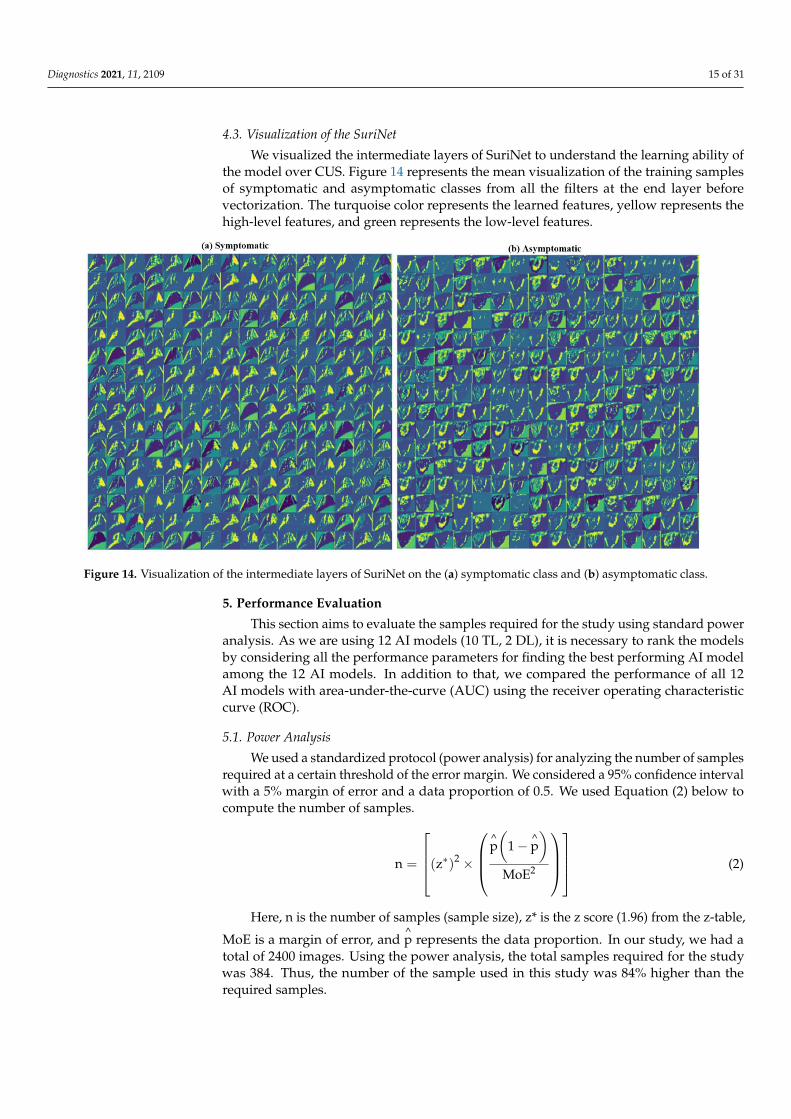
4.3. Visualization of the SuriNet

We visualized the intermediate layers of SuriNet to understand the learning ability ofthe model over CUS. Figure 14 represents the mean visualization of the training samplesof symptomatic and asymptomatic classes from all the filters at the end layer beforevectorization. The turquoise color represents the learned features, yellow represents thehigh-level features, and green represents the low-level features.


Figure 14. Visualization of the intermediate layers of SuriNet on the (a) symptomatic class and (b) asymptomatic class.

5. Performance Evaluation

This section aims to evaluate the samples required for the study using standard

power analysis. As we are using 12 AI models (10 TL, 2 DL), it is necessary to rank the

models by considering all the performance parameters for finding the best performing AI

model among the 12 AI models. In addition to that, we compared the performance of all

12 AI models with area-under-the-curve (AUC) using the receiver operating characteristic

curve (ROC).

5.1. Power Analysis

We used a standardized protocol (power analysis) for analyzing the number of sam-

ples required at a certain threshold of the error margin. We considered a 95% confidence

interval with a 5% margin of error and a data proportion of 0.5. We used Equation (2)

below to compute the number of samples.

n = [(z∗)2 × (p(1 − p)

MoE2)] (2)

Here, n is the number of samples (sample size), z* is the z score (1.96) from the z-

table, MoE is a margin of error, and p represents the data proportion. In our study, we

had a total of 2400 images. Using the power analysis, the total samples required for the

study was 384. Thus, the number of the sample used in this study was 84% higher than

the required samples.

5.2. Ranking of AI Models

After obtaining the absolute values of 12 AI models’ performance metrics, we sorted

the AI models into increasing order and then compared each value with the highest pos-

sible value in the attribute. We considered five marks. If the percentage was more signifi-

cant than 95%, we considered four marks. If it was greater than 90 and less than 95, we

considered three marks. If it was more significant than 80% and less than 90%, we consid-

ered two marks. If it was more significant than 75%, we considered one mark. If it was

greater than 50% or less than 50%, it was considered as zero. The resultant rank table of

the AI models is shown in Table 4. We color-coded each AI model from red to green. Each

Figure 14. Visualization of the intermediate layers of SuriNet on the (a) symptomatic class and (b) asymptomatic class.

5. Performance Evaluation

This section aims to evaluate the samples required for the study using standard poweranalysis. As we are using 12 AI models (10 TL, 2 DL), it is necessary to rank the modelsby considering all the performance parameters for finding the best performing AI modelamong the 12 AI models. In addition to that, we compared the performance of all 12AI models with area-under-the-curve (AUC) using the receiver operating characteristiccurve (ROC).

5.1. Power Analysis

We used a standardized protocol (power analysis) for analyzing the number of samplesrequired at a certain threshold of the error margin. We considered a 95% confidence intervalwith a 5% margin of error and a data proportion of 0.5. We used Equation (2) below tocompute the number of samples.

n =

(z∗)2 ×

^p(

1 − ^p)

MoE2

(2)

Here, n is the number of samples (sample size), z* is the z score (1.96) from the z-table,

MoE is a margin of error, and^p represents the data proportion. In our study, we had a

total of 2400 images. Using the power analysis, the total samples required for the studywas 384. Thus, the number of the sample used in this study was 84% higher than therequired samples.

Diagnostics 2021, 11, 2109 16 of 31

5.2. Ranking of AI Models

After obtaining the absolute values of 12 AI models’ performance metrics, we sortedthe AI models into increasing order and then compared each value with the highest possiblevalue in the attribute. We considered five marks. If the percentage was more significant than95%, we considered four marks. If it was greater than 90 and less than 95, we consideredthree marks. If it was more significant than 80% and less than 90%, we considered twomarks. If it was more significant than 75%, we considered one mark. If it was greaterthan 50% or less than 50%, it was considered as zero. The resultant rank table of the AImodels is shown in Table 4. We color-coded each AI model from red to green. Each modelis color-coded in this band. If the model performance is low, it is represented as red. If itperforms well, it is represented as green. Please see Appendix B for grading scheme.

Table 4. Ranking table of the AI models. The background color tells about the intensity of the classifier.

Rank Model O A F F1 Se Sp DS D TT Me AUC AS %1 VGG19 5 3 4 5 5 4 5 5 3 1 3 43 78.182 MobileNet 2 5 4 3 5 4 1 4 5 5 5 43 78.183 CNN11 * 4 5 2 4 5 4 4 5 1 3 5 42 76.364 AlexNet 5 4 2 2 2 2 5 3 4 3 3 35 63.605 Inception 1 3 5 5 4 5 1 5 1 1 3 34 61.826 DenseNet169 1 5 4 3 3 4 1 3 2 3 5 34 61.827 XceptionNet 5 3 2 2 3 2 5 0 3 4 3 32 58.188 SuriNet 2 3 3 3 4 3 3 3 3 3 30 54.559 VGG16 5 1 3 3 3 3 5 1 4 1 1 30 54.5510 SqueezeNet 2 2 3 3 3 3 4 1 2 3 2 28 50.9011 DenseNet 121 4 2 2 2 3 2 4 0 2 3 2 26 47.2712 ResNet50 3 2 2 2 3 2 3 0 1 3 2 23 41.80

O: optimization, A: accuracy, F: false positive rate, F1: F1 score, Se: sensitivity, Sp: specificity, DS: data size, D:DOR, TT: training time, Me: memory, AUC: area-under-the-curve AS: absolute score. * Note that CNN11 (rank 3)was used for benchmarking against other models (1, 2, and 4–12).

5.3. AUC-ROC Analysis

We computed the area-under-the-curve (AUC) for all the proposed AI models andcompared the performance with our previous existing work [62] consisting of a CNN modelwith an accuracy of 95.66% and AUC of 0.956. Figure 15 represents the ROC comparison of10 AI methods. Among all the architectures, MobileNet showed the highest AUC value as0.961 (p-value < 0.0001) and better performance than CNN [62].


model is color-coded in this band. If the model performance is low, it is represented as

red. If it performs well, it is represented as green. Please see Appendix B for grading

scheme.

Table 4. Ranking table of the AI models. The background color tells about the intensity of the clas-

sifier.

Rank Model O A F F1 Se Sp DS D TT Me AUC AS %

1 VGG19 5 3 4 5 5 4 5 5 3 1 3 43 78.18

2 MobileNet 2 5 4 3 5 4 1 4 5 5 5 43 78.18

3 CNN11 * 4 5 2 4 5 4 4 5 1 3 5 42 76.36

4 AlexNet 5 4 2 2 2 2 5 3 4 3 3 35 63.60

5 Inception 1 3 5 5 4 5 1 5 1 1 3 34 61.82

6 DenseNet169 1 5 4 3 3 4 1 3 2 3 5 34 61.82

7 XceptionNet 5 3 2 2 3 2 5 0 3 4 3 32 58.18

8 SuriNet 2 3 3 3 4 3 3 3 3 3 30 54.55

9 VGG16 5 1 3 3 3 3 5 1 4 1 1 30 54.55

10 SqueezeNet 2 2 3 3 3 3 4 1 2 3 2 28 50.90

11 DenseNet 121 4 2 2 2 3 2 4 0 2 3 2 26 47.27

12 ResNet50 3 2 2 2 3 2 3 0 1 3 2 23 41.80

O: optimization, A: accuracy, F: false positive rate, F1: F1 score, Se: sensitivity, Sp: specificity, DS:

data size, D: DOR, TT: training time, Me: memory, AUC: area-under-the-curve AS: absolute score.

* Note that CNN11 (rank 3) was used for benchmarking against other models (1, 2, and 4–12).

5.3. AUC-ROC Analysis

We computed the area-under-the-curve (AUC) for all the proposed AI models and

compared the performance with our previous existing work [62] consisting of a CNN

model with an accuracy of 95.66% and AUC of 0.956. Figure 15 represents the ROC com-

parison of 10 AI methods. Among all the architectures, MobileNet showed the highest

AUC value as 0.961 (p-value < 0.0001) and better performance than CNN [62].

False Postive Rate

ResNet50

VGG-16

SqueezeNet

DenseNet121

XceptionNet

Inception V3

AlexNet

VGG19

SuriNet

DenseNet169

DCNN

MobileNet

(0.780, p<0.0001)

(0.791, p<0.0001)

(0.832, p<0.0001)

(0.851, p<0.0001)

(0.851, p<0.0001)

(0.912, p<0.0001)

(0.915, p<0.0001)

(0.915, p<0.0001)

(0.927, p<0.0001)

(0.956, p<0.0001)

(0.956, p<0.0001)

(0.961, p<0.0001)

ROC Curve of 12 AI Methods

0.0 0.2 0.4 0.6 0.8 1.00.0

0.2

0.4

0.6

Tru

e P

ost

ive

Rate

0.8

1.0

Figure 15. ROC comparison of 12 AI models (10 TL and 2 DL). Figure 15. ROC comparison of 12 AI models (10 TL and 2 DL).

Diagnostics 2021, 11, 2109 17 of 31

6. Scientific Validation versus Clinical Validation

In this section, we discussed the validation of the hypothesis. Scientific validation wascarried out by heatmap analysis using the TL-based “Grad Cam” technique and clinicalvalidation was proved using a correlation analysis of the biomarker with AI.

6.1. Scientific Validation Using Heatmaps

We applied a novel visualization technique called gradient weighted class activationmap (“Grad Cam”) for identifying the diseased areas in the plaque cut sections usingVGG16 transfer learning architecture. Grad-CAM produces heatmaps based on the weightsgenerated during the training. Here, we take feature maps of the final layer. It gives theessential regions of the target, and heatmaps highlight these regions. Figures 16 and 17represent the heatmaps of the nine patients of symptomatic and asymptomatic class. Thedark red color region represents the diseased region in symptomatic plaque, whereas itrepresents the higher calcium area in asymptomatic plaque.

The Grad-Cam works on the training weights generated during the training phase. TheDL model captures the important regions of the target label. We compared the heatmapswith original images of both symptomatic and asymptomatic images. We observed thatheatmaps exhibit a darker region surrounded by grayscale regions. Meanwhile, in asymp-tomatic regions, DL observes grayscale regions. Figure 17(a1,a2,b1,c1) are the importantregions observed by DL of symptomatic images, and Figure 17(d1,e1,e2,e3,f1,f2,f3) arethe observed important regions of the asymptomatic images by the DL model. This com-parison proves our hypothesis that symptomatic plaques are hypoechoic and dark, andasymptomatic plaques are bright and hyperechoic.

6.2. Correlation Analysis

We correlated all the biomarkers for the detection of the risk with AI. Table 5 representsthe correlation coefficient of all the biomarkers. Among all the biomarkers, GSM versusFD shows a better p-value. We computed the correlation coefficient using MedCalc. Wecomputed the Euclidean distance (ED) between the centers of the two clusters (sym andasym). Table 6 represents the ED between two clusters, symptomatic versus asymptomatic.AI shows constant variation among all the techniques, whereas GSM with FD and higherorder spectra (HOS) shows the maximum distance. Figure 18 represents the correlationof AI (SuriNet), GSM, FD, and HOS, and the black dot represents the center of each class.The clusters of symptomatic and asymptomatic are represented with red and violet color,respectively. The black dot represents the center of the cluster and the eclipse on thecluster represents the high-density area. Figure 18b,d,e represent the (a) strong correlation,(c) moderate correlation, and (f) weak correlation between the biomarkers.

Table 5. Correlation analysis.

Symptomatic AsymptomaticComparison

CC p-Value CC p-ValueAbs.

Difference

FD vs. HOS 0.07221 0.0149 0.156 0.0017 1.160366

FD vs. GSM −0.241 <0.0001 −0.383 <0.0001 0.589212

GSM vs. HOS 0.0725 0.0147 −0.0630 0.0208 1.868966

SuriNet vs. GSM 0.0017 0.009 −0.0437 0.0031 26.70588

SuriNet vs. HOS −0.0234 0.006 −0.0394 0.0042 0.683761

SuriNet vs. FD 0.0623 0.0021 0.01347 0.0079 0.783788


Figure 16. Heat maps of the symptomatic plaque (left) and asymptomatic plaque (right). Figure 16. Heat maps of the symptomatic plaque (left) and asymptomatic plaque (right).

Table 6. Euclidean distance between biomarker pairs.

Comparison Euclidean DistanceSuriNet vs. FD 9.82

SuriNet vs. GSM 9.83

SuriNet vs. HOS 8.83

FD vs. GSM 24.20

GSM vs. HOS 24.19

FD vs. HOS 2.18


Figure 17. (a–c) The symptomatic image heatmaps vs. original images; (d–f) the asymptomatic image heatmaps vs. original

images (red color arrow represents the important regions).

6.2. Correlation Analysis

We correlated all the biomarkers for the detection of the risk with AI. Table 5 repre-

sents the correlation coefficient of all the biomarkers. Among all the biomarkers, GSM

versus FD shows a better p-value. We computed the correlation coefficient using MedCalc.

We computed the Euclidean distance (ED) between the centers of the two clusters (sym

and asym). Table 6 represents the ED between two clusters, symptomatic versus asymp-

tomatic. AI shows constant variation among all the techniques, whereas GSM with FD

and higher order spectra (HOS) shows the maximum distance. Figure 18 represents the

correlation of AI (SuriNet), GSM, FD, and HOS, and the black dot represents the center of

each class. The clusters of symptomatic and asymptomatic are represented with red and

violet color, respectively. The black dot represents the center of the cluster and the eclipse

on the cluster represents the high-density area. Figure 18b,d,e represent the (a) strong cor-

relation, (c) moderate correlation, and (f) weak correlation between the biomarkers.

Figure 17. (a–c) The symptomatic image heatmaps vs. original images; (d–f) the asymptomatic image heatmaps vs. originalimages (red color arrow represents the important regions).


Table 5. Correlation analysis.

Comparison Symptomatic Asymptomatic Abs.

Difference CC p-Value CC p-Value

FD vs. HOS 0.07221 0.0149 0.156 0.0017 1.160366

FD vs. GSM −0.241 <0.0001 −0.383 <0.0001 0.589212

GSM vs. HOS 0.0725 0.0147 −0.0630 0.0208 1.868966

SuriNet vs. GSM 0.0017 0.009 −0.0437 0.0031 26.70588

SuriNet vs. HOS −0.0234 0.006 −0.0394 0.0042 0.683761

SuriNet vs. FD 0.0623 0.0021 0.01347 0.0079 0.783788

Table 6. Euclidean distance between biomarker pairs.

Comparison Euclidean Distance

SuriNet vs. FD 9.82

SuriNet vs. GSM 9.83

SuriNet vs. HOS 8.83

FD vs. GSM 24.20

GSM vs. HOS 24.19

FD vs. HOS 2.18

Figure 18. Correlation of AI (SuriNet) and the three biomarkers—FD, GSM, and HOS (a) FD vs. SuriNet, (b) GSM vs.

SuriNet, (c) HOS vs. SuriNet, (d) FD vs. GSM, (e) HOS vs. GSM, and (f) FD vs. HOS.

7. Discussion

The proposed study is the first of its kind to use ten transfer learning models that

classify and characterize the symptomatic and asymptomatic carotid plaques. The pro-

posed models, 10 TL and 1 DL (SuriNet), are optimized using augmentation folds with K10 cross-validation protocol. The proposed MobileNet showed an accuracy of 96.19%,

while SuriNet was relatively high, having an accuracy of 92.70%, and our previous study

using CNN [62] showed 95.66%. Our overall performance analysis showed that TL per-

formance is superior to that of the DL models.

Figure 18. Correlation of AI (SuriNet) and the three biomarkers—FD, GSM, and HOS (a) FD vs. SuriNet, (b) GSM vs.SuriNet, (c) HOS vs. SuriNet, (d) FD vs. GSM, (e) HOS vs. GSM, and (f) FD vs. HOS.

Diagnostics 2021, 11, 2109 20 of 31

7. Discussion

The proposed study is the first of its kind to use ten transfer learning models thatclassify and characterize the symptomatic and asymptomatic carotid plaques. The proposedmodels, 10 TL and 1 DL (SuriNet), are optimized using augmentation folds with K10 cross-validation protocol. The proposed MobileNet showed an accuracy of 96.19%, while SuriNetwas relatively high, having an accuracy of 92.70%, and our previous study using CNN [62]showed 95.66%. Our overall performance analysis showed that TL performance is superiorto that of the DL models.

7.1. Benchmarking

In this section, we benchmarked the proposed system with the existingtechniques [29,58–63,74–84]. Table 7 shows the benchmarking table, where the table canbe classified into ML-based and DL-based systems for PTC. The table shows columns C1 toC6, where C1 represents the author and the corresponding year, C2 shows the selected featuresfor that study, C3 shows the classifiers used for PTC, C4 displays the dataset size and country,and C5 and C6 give the type of AI model and accuracy along with the AUC. Rows R1 to R17represent the existing studies on PTC using CUS, while R18 and R19 discuss the proposedstudies. In row R1, Christodoulou et al. [76] extracted ten different law texture energy featuresand fractal dimension features from the CUS and were able to characterize the PTC with diag-nostic yield (DY) of 73.1% using SOM and 68.8% using k-NN. Mougiakakou et al. (2006) [44](R2, C1) extracted first-order statistics and the law of texture energy features from 108 US scans.The authors reduced the dimensionality of the extracted features using ANOVA and thenfed the resultant features to neural networks with backpropagation and genetic architectureto classify symptomatic versus asymptomatic plaques. The authors achieved an accuracy of99.18% and 94.48%, respectively. Seabra et al. [74] (R3, C1) extracted echo-morphological andtexture features from 146 US scans. Then, they fused those features with clinical information,later used by AdaBoost classifier for classifying symptomatic versus asymptomatic plaques.The authors successfully achieved 99.2% accuracy using leave-one-participant-out (LOPO)cross-validation.

Table 7. Benchmarking table.

C1 C2 C3 C4 C5 C6SN#

Authors, Year FeaturesSelected

ClassifierType Dataset AI Type ACC. (%)

AUC (p-Value)

R1 Christodoulouet al. (2003) [76]

TextureFeatures

SOMKNN

230(-) ML 73.18, 68.88,

0.753, 0.738

R2 Mougiakakouet al. (2006) [77]

FOS andTextureFeatures

NN with BPand GA

108(UK) ML

99.18,94.48,0.918

R3 Seabra et al.2010 [74] Five Features Adaboost using

LOPO 146 Patients ML 99.2

R4Christodoulou

et al.2010 [79]

Shape Features,Morphology

Features,HistogramFeatures,

CorrelogramFeatures

SOMKNN 274 Patients ML 72.6,

73.0

R5 Acharya et al.(2011) [58]

TextureFeatures

SVM with RBFAdaboost

346(Cyprus) ML

82.48,81.78,

0.818, 0.810p < 0.0001

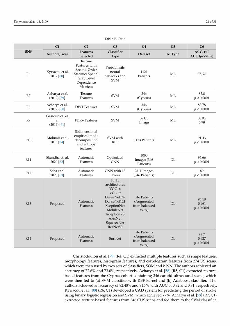
Diagnostics 2021, 11, 2109 21 of 31

Table 7. Cont.

C1 C2 C3 C4 C5 C6SN#

Authors, Year FeaturesSelected

ClassifierType Dataset AI Type ACC. (%)

AUC (p-Value)

R6 Kyriacou et al.2012 [80]

TextureFeatures withSecond-Order

Statistics SpatialGray Level

DependenceMatrices

Probabilisticneural

networks andSVM

1121Patients ML 77, 76

R7 Acharya et al.(2012) [59]

TextureFeatures SVM 346

(Cyprus) ML 83.8p < 0.0001

R8 Acharya et al.,(2012) [60] DWT Features SVM 346

(Cyprus) ML 83.78p < 0.0001

R9Gastounioti et.

al.(2014) [61]

FDR+ Features SVM 56 USImage ML 88.08,

0.90

R10 Molinari et al.2018 [84]

Bidimensionalempirical modedecomposition

and entropyfeatures

SVM withRBF 1173 Patients ML 91.43

p < 0.0001

R11 Skandha et. al.2020 [62]

AutomaticFeatures

OptimizedCNN

2000Images (346

Patients)DL 95.66

p < 0.0001

R12 Saba et al.2020 [63]

AutomaticFeatures

CNN with 13layers

2311 Images(346 Patients) DL 89

p < 0.0001

R13 Proposed AutomaticFeatures

10 TLarchitectures

VGG16VGG19

DenseNet169DenseNet121XceptionNetMobileNet

InceptionV3AlexNet

SqueezeNetResNet50

346 Patients(Augmented

from balancedto 6x)

DL96.180.961

p < 0.0001

R14 Proposed AutomaticFeatures SuriNet

346 Patients(Augmented

from balancedto 6x)

DL92.7

0.927p < 0.0001

Christodoulou et al. [79] (R4, C1) extracted multiple features such as shape features,morphology features, histogram features, and correlogram features from 274 US scans,which were then used by two sets of classifiers, SOM and k-NN. The authors achieved anaccuracy of 72.6% and 73.0%, respectively. Acharya et al. [58] (R5, C1) extracted texture-based features from the Cyprus cohort containing 346 carotid ultrasound scans, whichwere then fed to (a) SVM classifier with RBF kernel and (b) Adaboost classifier. Theauthors achieved an accuracy of 82.48% and 81.7% with AUC of 0.82 and 0.81, respectively.Kyriacou et al. [80] (R6, C1) developed a CAD system for predicting the period of strokeusing binary logistic regression and SVM, which achieved 77%. Acharya et al. [59] (R7, C1)extracted texture-based features from 346 CUS scans and fed them to the SVM classifier,

Diagnostics 2021, 11, 2109 22 of 31

and achieved an accuracy of 83.78%. The same authors in [60] (R8, C1) extracted discretewavelet transform (DWT) features using the Cyprus cohort of 346 US scans, and fed themto an SVM classifier, achieving an accuracy of 83.78%. Gatounioti et al. [61] (R9, C1)extracted Fisher discriminant ratio features from 56 CUS scans, and fed them to an SVMclassifier, achieving an accuracy of 88.08% with an AUC of 0.90. Molinari et al. [84] (R10,C1) used a data mining approach by taking bidimensional empirical mode decompositionand entropy features from 1173 CUS scans and then used an SVM classifier with RBF kernelfor classification. The authors achieved an accuracy of 91.43%.

The second set of studies used DL models for PTC. Skandha et al. [62] (R11, C1)extracted automatic features using optimized CNN from augmented 346 patients. Theauthors achieved an accuracy of 95.66% and an AUC of 0.956 (p < 0.0001). The authorssuccessfully characterized the symptomatic versus asymptomatic plaques using meanfeature strength, higher-order spectrum, and histogram analysis. Saba et al. [63] (R12, C1)used a randomized augmented cohort generated from 346 patient CUS with 13 layeredCNN and achieved an accuracy of 89% with an AUC of 0.9 (p < 0.0001).

7.2. Comparison of TL Models

TL architectures use the pretrained weights for retraining the model for target labelprediction. However, the TL architecture training time depended on the size of the pre-trained weights and hardware resources. Various TL models discussed in Table 6 hadadvantages over the other model, as explained in Tables 8 and 9.

Table 8. Comparison of TL models.

SN# Author, Year Name of theNetwork Dataset Purpose

PretrainedWeight Size

(MB)

Typeof

Layers

1 Krizhevskyet al., 2012 [72] AlexNet ImageNet Classification 244

Convolution,Max Pooling,

FCN

2 Simonyan et al.,2015 [66] VGG -16, 19 ImageNet Object

recognition 528, 549Convolution,Max Pooling,

FCN

3 Szegedy et al.,2015 [69] InceptionV3 ImageNet Object

recognition 92


Inception,FCN

4 He et al.,2016 [70]

ResNet 50, 101,and 152

ImageNet,CIFAR

Fastoptimizationfor extremelydeep neural

networks

98,171, 232

Convolution,Avg Pooling,

Residual,FCN

5 Howard et al.,2017 [42] MobileNet ImageNet

Classificationand

segmentationin mobiles

16

Convolution,Depth-wise

Convolution,Average Pooling,

FCN

6 Chollet et al.,2017 [71] XceptionNet ImageNet,

JFT

Modifieddepthwiseseparable

convolution.Advancement

ofInceptionV3

88

Convolution,Separable


Global Avg Pooling,FCN

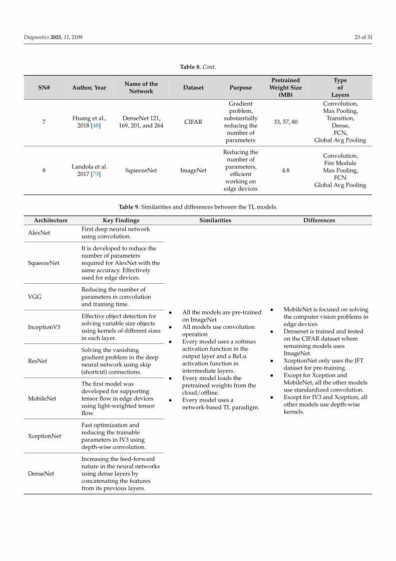
Diagnostics 2021, 11, 2109 23 of 31

Table 8. Cont.

SN# Author, Year Name of theNetwork Dataset Purpose

PretrainedWeight Size

(MB)

Typeof

Layers

7 Huang et al.,2018 [48]

DenseNet 121,169, 201, and 264 CIFAR

Gradientproblem,

substantiallyreducing thenumber ofparameters

33, 57, 80


Transition,Dense,FCN,

Global Avg Pooling

8 Landola et al.2017 [73] SqueezeNet ImageNet

Reducing thenumber of

parameters,efficient

working onedge devices

4.8

Convolution,Fire ModuleMax Pooling,

FCNGlobal Avg Pooling

Table 9. Similarities and differences between the TL models.

Architecture Key Findings Similarities Differences

AlexNet First deep neural networkusing convolution.

• All the models are pre-trainedon ImageNet

• All models use convolutionoperation

• Every model uses a softmaxactivation function in theoutput layer and a ReLuactivation function inintermediate layers.

• Every model loads thepretrained weights from thecloud/offline.

• Every model uses anetwork-based TL paradigm.

• MobileNet is focused on solvingthe computer vision problems inedge devices

• Densenet is trained and testedon the CIFAR dataset whereremaining models usesImageNet.

• XceptionNet only uses the JFTdataset for pre-training.

• Except for Xception andMobileNet, all the other modelsuse standardized convolution.

• Except for IV3 and Xception, allother models use depth-wisekernels.

SqueezeNet

It is developed to reduce thenumber of parametersrequired for AlexNet with thesame accuracy. Effectivelyused for edge devices.

VGGReducing the number ofparameters in convolutionand training time.

InceptionV3

Effective object detection forsolving variable size objectsusing kernels of different sizesin each layer.

ResNet

Solving the vanishinggradient problem in the deepneural network using skip(shortcut) connections.

MobileNet

The first model wasdeveloped for supportingtensor flow in edge devicesusing light-weighted tensorflow.

XceptionNet

Fast optimization andreducing the trainableparameters in IV3 usingdepth-wise convolution.

DenseNet

Increasing the feed-forwardnature in the neural networksusing dense layers byconcatenating the featuresfrom its previous layers.

Diagnostics 2021, 11, 2109 24 of 31

7.3. Advantages of TL Models

TL models’ designs have similarities and differences between them. These are ex-plained in Table 9, along the key findings of every TL model.

7.4. GUI Design

AtheroPoint™ developed the Atheromatic™ 2.0 TL system, a computer-aided diag-nostic system for stroke risk stratification. Figure 19 represents the screenshot of the CADsystem. This CAD system will provide the plaque risk and heatmaps generated by theGrad-Cam with the help of TL/DL models. In the CAD system, the heatmap would bepredicted on the test image once the training model is selected.


7.4. GUI Design

AtheroPoint™ developed the Atheromatic™ 2.0 TL system, a computer-aided diag-

nostic system for stroke risk stratification. Figure 19 represents the screenshot of the CAD

system. This CAD system will provide the plaque risk and heatmaps generated by the

Grad-Cam with the help of TL/DL models. In the CAD system, the heatmap would be

predicted on the test image once the training model is selected.

Figure 19. GUI screenshot of the Atheromatic™ 2.0 TL system.

7.5. Strengths/Weakness/Extensions

We evaluated the optimization point of the TL models against various augmentation

folds and compared the performance of the TL models against that of the DL models such

as SuriNet and CNN. The TL model showed an improvement for symptomatic versus

asymptomatic plaque classification accuracy. Furthermore, our Atheromatic™ 2.0 TL sys-

tem predicts the risk of plaque and vulnerability using the color heatmaps on test scans.

Even though the power sample suggests that we have enough samples for the train-

ing, the main limitation of this study was the moderate cohort size. In addition to the

cohort size, another limitation of this study is the limited availability of the hardware re-

sources such as supercomputer availability, especially in third-world developing coun-

tries.

Our study had a manual delineation of ICA data sets. In future, there could be a need

to design an automated ICA segmentation system [85]. Another possibility would be to

improve the CNN by an improved DCNN model, where the rectified linear unit (ReLU)

activation function was modified, ensuring “differentiable at zero” [38]. There are dense

networks such as DenseNet121, DenseNet169, and DenseNet201 that could be tried and

compared [39]. Further, one can further combine hybrid deep learning models for PTC

[86]. Finally, the proposed AI models can be extended to a big data framework by includ-

ing other risk factors.

8. Conclusions

Figure 19. GUI screenshot of the Atheromatic™ 2.0 TL system with three example cases (a–c).

7.5. Strengths/Weakness/Extensions

We evaluated the optimization point of the TL models against various augmentationfolds and compared the performance of the TL models against that of the DL modelssuch as SuriNet and CNN. The TL model showed an improvement for symptomaticversus asymptomatic plaque classification accuracy. Furthermore, our Atheromatic™ 2.0 TLsystem predicts the risk of plaque and vulnerability using the color heatmaps on test scans.

Even though the power sample suggests that we have enough samples for the training,the main limitation of this study was the moderate cohort size. In addition to the cohortsize, another limitation of this study is the limited availability of the hardware resourcessuch as supercomputer availability, especially in third-world developing countries.

Our study had a manual delineation of ICA data sets. In future, there could be a needto design an automated ICA segmentation system [85]. Another possibility would be toimprove the CNN by an improved DCNN model, where the rectified linear unit (ReLU)activation function was modified, ensuring “differentiable at zero” [38]. There are densenetworks such as DenseNet121, DenseNet169, and DenseNet201 that could be tried andcompared [39]. Further, one can further combine hybrid deep learning models for PTC [86].Finally, the proposed AI models can be extended to a big data framework by includingother risk factors.

Diagnostics 2021, 11, 2109 25 of 31

8. Conclusions

The proposed study is the first of its kind to characterize and classify the carotid plaqueusing an optimized transfer learning approach and SuriNet (a class of Atheromatic™ 2.0TL). Eleven AItherop models were implemented, and the best AUC was 0.961 (p < 0.0001)from MobileNet and 0.927 (p < 0.0001) from SuriNet. We validated the performanceusing grayscale median, fractal dimension, higher-order spectra, and spatial heatmaps.TL showed equal and comparable performance to deep learning. The Atheromatic™2.0 TL model showed a performance improvement of 12.9% over Atheromatic™ 1.0ML(AtheroPoint, Roseville, CA, USA) compared with the previous machine learning-basedparadigm. The system was validated with the widely accepted dataset.

Author Contributions: Conceptualization, J.S.S., S.S.S.; methodology, S.S.S., A.N., S.K.G. and V.K.K.;software, V.K.K., L.S. and S.A.; validation, A.N., L.S., S.A., A.M.J. and M.S.K.; formal analysis, S.S.S.,J.S.S. and L.S.; investigation, S.S.S., L.S. and J.S.S.; resources, A.N., S.K.G., V.K.K. and L.S.; datacuration, S.S.S. and J.S.S.; writing—original draft preparation, S.S.S., A.N., S.K.G., V.K.K., LS, S.A.,A.M.J. and J.S.S.; writing—review and editing, S.S.S., A.N., S.K.G., V.K.K., L.S., S.A., A.M.J., M.S.K.and J.S.S.; visualization S.S.S. and V.K.K.; supervision, S.K.G., V.K.K. and J.S.S.; project administration,J.S.S.; All authors have read and agreed to the published version of the manuscript.

Funding: This research received no external funding.

Institutional Review Board Statement: The study was approved by the ethical committee of St.Mary’s Hospital, Imperial College, London, UK (2000).

Informed Consent Statement: Informed consent was obtained from all subjects involved in the study.

Conflicts of Interest: Dr. Jasjit Suri is with AtheropointTM specialization in cardiovascular and strokeimaging. The rest of the authors declare no conflict of interest.

Abbreviations

Symbol AbbreviationAcc AccuracyAF Amaurosis fugaxAI Artificial intelligenceAPSI Atheromatic plaque separation indexAsym Asymptomatic plaqueAUC Area-under-the-curveCAD Computer-aided diagnosticCT Computed tomographyCV Cross-validationCVD Cardiovascular diseaseDCNN Deep convolutional neural networkDL Deep learningDOR Diagnostics odds ratioDWT Discrete wavelets transformDY Diagnostic yieldEAI Enhanced activity indexED Euclidean distanceFC, FCN Fully connected networkFD Fractal dimensionFN Fine-tune networksGLDS Gray level difference statisticGrad-Cam Gradient-weighted class activation mapGSM Greyscale medianICA Internal carotid arteryIV3 Inception V3k-NN K-nearest neighborLOPO Leave-one-participant-out

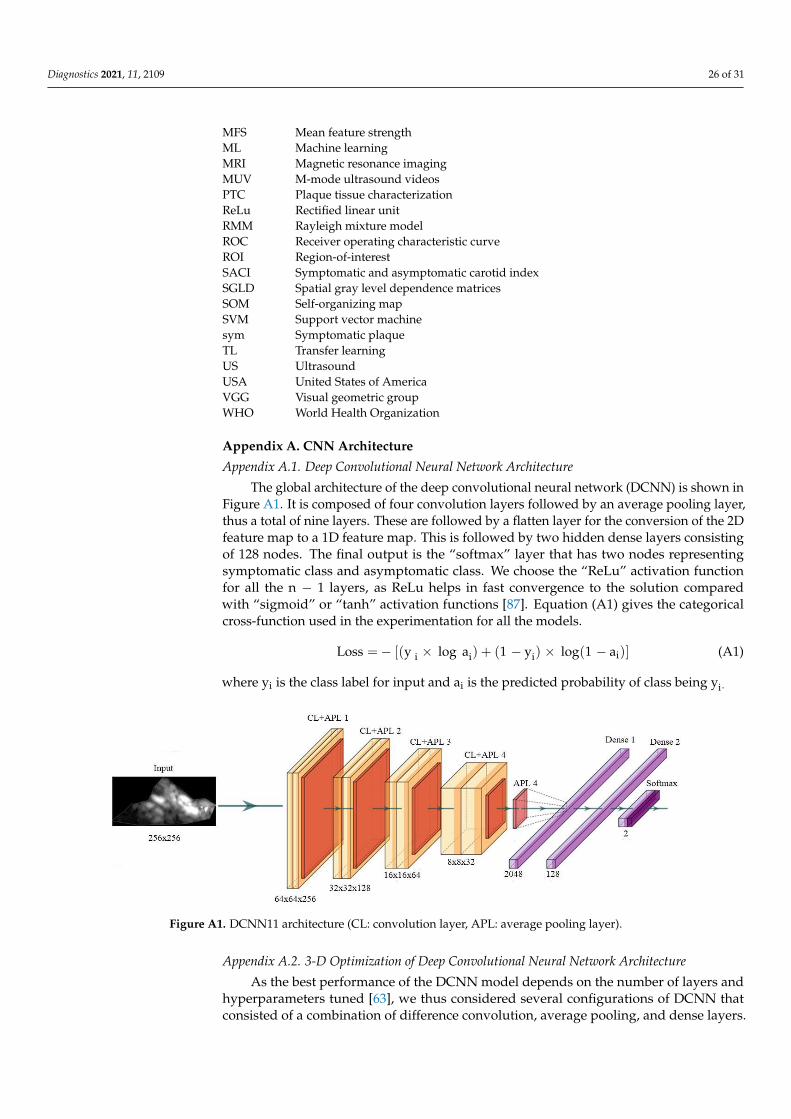
Diagnostics 2021, 11, 2109 26 of 31

MFS Mean feature strengthML Machine learningMRI Magnetic resonance imagingMUV M-mode ultrasound videosPTC Plaque tissue characterizationReLu Rectified linear unitRMM Rayleigh mixture modelROC Receiver operating characteristic curveROI Region-of-interestSACI Symptomatic and asymptomatic carotid indexSGLD Spatial gray level dependence matricesSOM Self-organizing mapSVM Support vector machinesym Symptomatic plaqueTL Transfer learningUS UltrasoundUSA United States of AmericaVGG Visual geometric groupWHO World Health Organization

Appendix A. CNN Architecture

Appendix A.1. Deep Convolutional Neural Network Architecture

The global architecture of the deep convolutional neural network (DCNN) is shown inFigure A1. It is composed of four convolution layers followed by an average pooling layer,thus a total of nine layers. These are followed by a flatten layer for the conversion of the 2Dfeature map to a 1D feature map. This is followed by two hidden dense layers consistingof 128 nodes. The final output is the “softmax” layer that has two nodes representingsymptomatic class and asymptomatic class. We choose the “ReLu” activation functionfor all the n − 1 layers, as ReLu helps in fast convergence to the solution comparedwith “sigmoid” or “tanh” activation functions [87]. Equation (A1) gives the categoricalcross-function used in the experimentation for all the models.

Loss =− [(y i × log ai) + (1 − yi) × log(1 − ai)] (A1)

where yi is the class label for input and ai is the predicted probability of class being yi.


ML Machine learning

MRI Magnetic resonance imaging

MUV M-mode ultrasound videos

PTC Plaque tissue characterization

ReLu Rectified linear unit

RMM Rayleigh mixture model

ROC Receiver operating characteristic curve

ROI Region-of-interest

SACI Symptomatic and asymptomatic carotid index

SGLD Spatial gray level dependence matrices

SOM Self-organizing map

SVM Support vector machine

sym Symptomatic plaque

TL Transfer learning

US Ultrasound

USA United States of America

VGG Visual geometric group

WHO World Health Organization

Appendix A. CNN Architecture

Appendix A.1. Deep Convolutional Neural Network Architecture

The global architecture of the deep convolutional neural network (DCNN) is shown

in Figure A1. It is composed of four convolution layers followed by an average pooling

layer, thus a total of nine layers. These are followed by a flatten layer for the conversion

of the 2D feature map to a 1D feature map. This is followed by two hidden dense layers

consisting of 128 nodes. The final output is the “softmax” layer that has two nodes repre-

senting symptomatic class and asymptomatic class. We choose the “ReLu” activation

function for all the n 1 layers, as ReLu helps in fast convergence to the solution compared

with “sigmoid” or “tanh” activation functions [87]. Equation (A1) gives the categorical

cross-function used in the experimentation for all the models.

Loss = − [(yi × log ai) + (1 − y

i) × log(1 − a

i)] (A1)

where yi is the class label for input and ai is the predicted probability of class being yi.

Figure A1. DCNN11 architecture (CL: convolution layer, APL: average pooling layer).

Appendix A.2. 3-D Optimization of Deep Convolutional Neural Network Architecture

As the best performance of the DCNN model depends on the number of layers and

hyperparameters tuned [63], we thus considered several configurations of DCNN that

consisted of a combination of difference convolution, average pooling, and dense layers.

Figure A1. DCNN11 architecture (CL: convolution layer, APL: average pooling layer).

Appendix A.2. 3-D Optimization of Deep Convolutional Neural Network Architecture

As the best performance of the DCNN model depends on the number of layers andhyperparameters tuned [63], we thus considered several configurations of DCNN thatconsisted of a combination of difference convolution, average pooling, and dense layers.

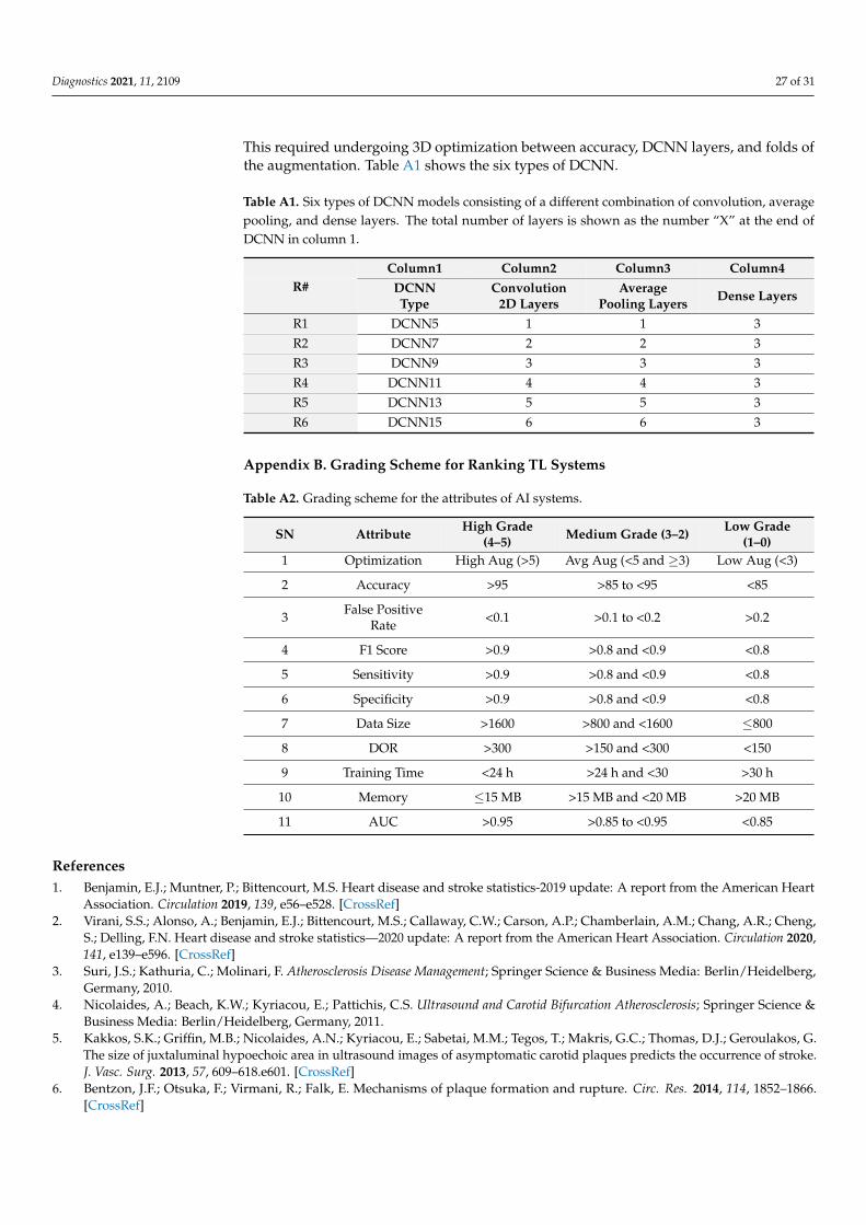
Diagnostics 2021, 11, 2109 27 of 31

This required undergoing 3D optimization between accuracy, DCNN layers, and folds ofthe augmentation. Table A1 shows the six types of DCNN.

Table A1. Six types of DCNN models consisting of a different combination of convolution, averagepooling, and dense layers. The total number of layers is shown as the number “X” at the end ofDCNN in column 1.

Column1 Column2 Column3 Column4R# DCNN

TypeConvolution

2D LayersAverage

Pooling Layers Dense Layers

R1 DCNN5 1 1 3R2 DCNN7 2 2 3R3 DCNN9 3 3 3R4 DCNN11 4 4 3R5 DCNN13 5 5 3R6 DCNN15 6 6 3

Appendix B. Grading Scheme for Ranking TL Systems

Table A2. Grading scheme for the attributes of AI systems.

SN Attribute High Grade(4–5) Medium Grade (3–2) Low Grade

(1–0)1 Optimization High Aug (>5) Avg Aug (<5 and ≥3) Low Aug (<3)

2 Accuracy >95 >85 to <95 <85

3 False PositiveRate <0.1 >0.1 to <0.2 >0.2

4 F1 Score >0.9 >0.8 and <0.9 <0.8

5 Sensitivity >0.9 >0.8 and <0.9 <0.8

6 Specificity >0.9 >0.8 and <0.9 <0.8

7 Data Size >1600 >800 and <1600 ≤800

8 DOR >300 >150 and <300 <150

9 Training Time <24 h >24 h and <30 >30 h

10 Memory ≤15 MB >15 MB and <20 MB >20 MB

11 AUC >0.95 >0.85 to <0.95 <0.85

References1. Benjamin, E.J.; Muntner, P.; Bittencourt, M.S. Heart disease and stroke statistics-2019 update: A report from the American Heart

Association. Circulation 2019, 139, e56–e528. [CrossRef]2. Virani, S.S.; Alonso, A.; Benjamin, E.J.; Bittencourt, M.S.; Callaway, C.W.; Carson, A.P.; Chamberlain, A.M.; Chang, A.R.; Cheng,

S.; Delling, F.N. Heart disease and stroke statistics—2020 update: A report from the American Heart Association. Circulation 2020,141, e139–e596. [CrossRef]

3. Suri, J.S.; Kathuria, C.; Molinari, F. Atherosclerosis Disease Management; Springer Science & Business Media: Berlin/Heidelberg,Germany, 2010.

4. Nicolaides, A.; Beach, K.W.; Kyriacou, E.; Pattichis, C.S. Ultrasound and Carotid Bifurcation Atherosclerosis; Springer Science &Business Media: Berlin/Heidelberg, Germany, 2011.

5. Kakkos, S.K.; Griffin, M.B.; Nicolaides, A.N.; Kyriacou, E.; Sabetai, M.M.; Tegos, T.; Makris, G.C.; Thomas, D.J.; Geroulakos, G.The size of juxtaluminal hypoechoic area in ultrasound images of asymptomatic carotid plaques predicts the occurrence of stroke.J. Vasc. Surg. 2013, 57, 609–618.e601. [CrossRef]

6. Bentzon, J.F.; Otsuka, F.; Virmani, R.; Falk, E. Mechanisms of plaque formation and rupture. Circ. Res. 2014, 114, 1852–1866.[CrossRef]

http://doi.org/10.1161/CIR.0000000000000659

http://doi.org/10.1161/CIR.0000000000000757

http://doi.org/10.1016/j.jvs.2012.09.045

http://doi.org/10.1161/CIRCRESAHA.114.302721

Diagnostics 2021, 11, 2109 28 of 31

7. Cuadrado-Godia, E.; Dwivedi, P.; Sharma, S.; Santiago, A.O.; Gonzalez, J.R.; Balcells, M.; Laird, J.; Turk, M.; Suri, H.S.; Nicolaides,A. cerebral small vessel disease: A review focusing on pathophysiology, biomarkers, and machine learning strategies. J. Stroke2018, 20, 302. [CrossRef]

8. Saba, L.; Gao, H.; Raz, E.; Sree, S.V.; Mannelli, L.; Tallapally, N.; Molinari, F.; Bassareo, P.P.; Acharya, U.R.; Poppert, H.Semiautomated analysis of carotid artery wall thickness in MRI. J. Magn. Reson. Imaging 2014, 39, 1457–1467. [CrossRef]

9. Saba, L.; Suri, J.S. Multi-Detector CT Imaging: Principles, Head, Neck, and Vascular Systems; CRC Press: Boca Raton, FL, USA, 2013;Volume 1.

10. Seabra, J.; Sanches, J. Ultrasound Imaging: Advances and Applications; Springer: Berlin/Heidelberg, Germany, 2012.11. Sanches, J.M.; Laine, A.F.; Suri, J.S. Ultrasound Imaging; Springer: Berlin/Heidelberg, Germany, 2012.12. Londhe, N.D.; Suri, J.S. Superharmonic imaging for medical ultrasound: A review. J. Med. Syst. 2016, 40, 279. [CrossRef]13. Hussain, M.A.; Saposnik, G.; Raju, S.; Salata, K.; Mamdani, M.; Tu, J.V.; Bhatt, D.L.; Verma, S.; Al-Omran, M. Association between

statin use and cardiovascular events after carotid artery revascularization. J. Am. Heart Assoc. 2018, 7, e009745. [CrossRef]14. Acharya, U.R.; Sree, S.V.; Ribeiro, R.; Krishnamurthi, G.; Marinho, R.T.; Sanches, J.; Suri, J.S. Data mining framework for fatty

liver disease classification in ultrasound: A hybrid feature extraction paradigm. Med. Phys. 2012, 39, 4255–4264. [CrossRef]15. Saba, L.; Dey, N.; Ashour, A.S.; Samanta, S.; Nath, S.S.; Chakraborty, S.; Sanches, J.; Kumar, D.; Marinho, R.; Suri, J.S. Automated

stratification of liver disease in ultrasound: An online accurate feature classification paradigm. Comput. Methods Programs Biomed.2016, 130, 118–134. [CrossRef]

16. Acharya, U.R.; Swapna, G.; Sree, S.V.; Molinari, F.; Gupta, S.; Bardales, R.H.; Witkowska, A.; Suri, J.S. A review on ultrasound-based thyroid cancer tissue characterization and automated classification. Technol. Cancer Res. Treat. 2014, 13, 289–301. [CrossRef]

17. Acharya, U.; Vinitha Sree, S.; Mookiah, M.; Yantri, R.; Molinari, F.; Zieleznik, W.; Małyszek-Tumidajewicz, J.; Stepien, B.; Bardales,R.; Witkowska, A. Diagnosis of Hashimoto’s thyroiditis in ultrasound using tissue characterization and pixel classification. Proc.Inst. Mech. Eng. Part H. J. Eng. Med. 2013, 227, 788–798. [CrossRef]

18. Acharya, U.R.; Sree, S.V.; Krishnan, M.M.R.; Molinari, F.; Garberoglio, R.; Suri, J.S. Non-invasive automated 3D thyroid lesionclassification in ultrasound: A class of ThyroScan™ systems. Ultrasonics 2012, 52, 508–520. [CrossRef]

19. Pareek, G.; Acharya, U.R.; Sree, S.V.; Swapna, G.; Yantri, R.; Martis, R.J.; Saba, L.; Krishnamurthi, G.; Mallarini, G.; El-Baz, A.Prostate tissue characterization/classification in 144 patient population using wavelet and higher order spectra features fromtransrectal ultrasound images. Technol. Cancer Res. Treat. 2013, 12, 545–557. [CrossRef]

20. McClure, P.; Elnakib, A.; El-Ghar, M.A.; Khalifa, F.; Soliman, A.; El-Diasty, T.; Suri, J.S.; Elmaghraby, A.; El-Baz, A. In-vitro andin-vivo diagnostic techniques for prostate cancer: A review. J. Biomed. Nanotechnol. 2014, 10, 2747–2777. [CrossRef]

21. Acharya, U.R.; Sree, S.V.; Kulshreshtha, S.; Molinari, F.; Koh, J.E.W.; Saba, L.; Suri, J.S. GyneScan: An improved online paradigmfor screening of ovarian cancer via tissue characterization. Technol. Cancer Res. Treat. 2014, 13, 529–539. [CrossRef]

22. Shrivastava, V.K.; Londhe, N.D.; Sonawane, R.S.; Suri, J.S. Computer-aided diagnosis of psoriasis skin images with HOS, textureand color features: A first comparative study of its kind. Comput. Methods Programs Biomed. 2016, 126, 98–109. [CrossRef]

23. Shrivastava, V.K.; Londhe, N.D.; Sonawane, R.S.; Suri, J.S. A novel and robust Bayesian approach for segmentation of psoriasislesions and its risk stratification. Comput. Methods Programs Biomed. 2017, 150, 9–22. [CrossRef]

24. Kaur, R.; GholamHosseini, H.; Sinha, R. Deep Learning in Medical Applications: Lesion Segmentation in Skin Cancer ImagesUsing Modified and Improved Encoder-Decoder Architecture. Geom. Vis. 2021, 1386, 39.

25. Sarker, M.M.K.; Rashwan, H.A.; Akram, F.; Singh, V.K.; Banu, S.F.; Chowdhury, F.U.; Choudhury, K.A.; Chambon, S.; Radeva, P.;Puig, D. SLSNet: Skin lesion segmentation using a lightweight generative adversarial network. Expert Syst. Appl. 2021, 115433.[CrossRef]

26. Maniruzzaman, M.; Kumar, N.; Abedin, M.M.; Islam, M.S.; Suri, H.S.; El-Baz, A.S.; Suri, J.S. Comparative approaches forclassification of diabetes mellitus data: Machine learning paradigm. Comput. Methods Programs Biomed. 2017, 152, 23–34.[CrossRef]

27. Maniruzzaman, M.; Rahman, M.J.; Al-MehediHasan, M.; Suri, H.S.; Abedin, M.M.; El-Baz, A.; Suri, J.S. Accurate diabetes riskstratification using machine learning: Role of missing value and outliers. J. Med. Syst. 2018, 42, 92. [CrossRef]

28. Acharya, U.R.; Sree, S.V.; Krishnan, M.M.R.; Krishnananda, N.; Ranjan, S.; Umesh, P.; Suri, J.S. Automated classification ofpatients with coronary artery disease using grayscale features from left ventricle echocardiographic images. Comput. MethodsPrograms Biomed. 2013, 112, 624–632. [CrossRef]

29. Acharya, U.R.; Mookiah, M.R.; Vinitha Sree, S.; Afonso, D.; Sanches, J.; Shafique, S.; Nicolaides, A.; Pedro, L.M.; e Fernandes, J.F.;Suri, J.S. Atherosclerotic plaque tissue characterization in 2D ultrasound longitudinal carotid scans for automated classification:A paradigm for stroke risk assessment. Med. Biol. Eng. Comput. 2013, 51, 513–523. [CrossRef]

30. Saba, L.; Jain, P.K.; Suri, H.S.; Ikeda, N.; Araki, T.; Singh, B.K.; Nicolaides, A.; Shafique, S.; Gupta, A.; Laird, J.R. Plaque tissuemorphology-based stroke risk stratification using carotid ultrasound: A polling-based PCA learning paradigm. J. Med. Syst. 2017,41, 98. [CrossRef]

31. Acharya, U.R.; Faust, O.; Alvin, A.; Krishnamurthi, G.; Seabra, J.C.; Sanches, J.; Suri, J.S. Understanding symptomatology ofatherosclerotic plaque by image-based tissue characterization. Comput. Methods Programs 2013, 110, 66–75. [CrossRef]

32. Acharya, R.U.; Faust, O.; Alvin, A.P.C.; Sree, S.V.; Molinari, F.; Saba, L.; Nicolaides, A.; Suri, J.S. Symptomatic vs. asymptomaticplaque classification in carotid ultrasound. J. Med. Syst. 2012, 36, 1861–1871. [CrossRef]

http://doi.org/10.5853/jos.2017.02922

http://doi.org/10.1002/jmri.24307

http://doi.org/10.1007/s10916-016-0635-x

http://doi.org/10.1161/JAHA.118.009745

http://doi.org/10.1118/1.4725759

http://doi.org/10.1016/j.cmpb.2016.03.016

http://doi.org/10.7785/tcrt.2012.500381

http://doi.org/10.1177/0954411913483637

http://doi.org/10.1016/j.ultras.2011.11.003

http://doi.org/10.7785/tcrt.2012.500346

http://doi.org/10.1166/jbn.2014.1990

http://doi.org/10.7785/tcrtexpress.2013.600273



http://doi.org/10.1016/j.eswa.2021.115433


http://doi.org/10.1007/s10916-018-0940-7


http://doi.org/10.1007/s11517-012-1019-0

http://doi.org/10.1007/s10916-017-0745-0


http://doi.org/10.1007/s10916-010-9645-2

Diagnostics 2021, 11, 2109 29 of 31

33. Saba, L.; Ikeda, N.; Deidda, M.; Araki, T.; Molinari, F.; Meiburger, K.M.; Acharya, U.R.; Nagashima, Y.; Mercuro, G.; Nakano, M.Association of automated carotid IMT measurement and HbA1c in Japanese patients with coronary artery disease. Diabetes Res.Clin. Pract. 2013, 100, 348–353. [CrossRef]

34. Saba, L.; Biswas, M.; Kuppili, V.; Godia, E.C.; Suri, H.S.; Edla, D.R.; Omerzu, T.; Laird, J.R.; Khanna, N.N.; Mavrogeni, S. Thepresent and future of deep learning in radiology. Eur. J. Radiol. 2019, 114, 14–24. [CrossRef]

35. Biswas, M.; Kuppili, V.; Saba, L.; Edla, D.; Suri, H.; Cuadrado-Godia, E.; Laird, J.; Marinhoe, R.; Sanches, J.; Nicolaides, A.State-of-the-art review on deep learning in medical imaging. Front. Biosci. 2019, 24, 392–426.

36. Sanagala, S.S.; Gupta, S.K.; Koppula, V.K.; Agarwal, M. A Fast and Light Weight Deep Convolution Neural Network Model forCancer Disease Identification in Human Lung(s). In Proceedings of the 2019 18th IEEE International Conference on MachineLearning And Applications (ICMLA), Boca Raton, FL, USA, 16–19 December 2019; pp. 1382–1387.

37. Tandel, G.S.; Balestrieri, A.; Jujaray, T.; Khanna, N.N.; Saba, L.; Suri, J.S. Multiclass magnetic resonance imaging brain tumorclassification using artificial intelligence paradigm. Comput. Biol. Med. 2020, 122, 103804. [CrossRef]

38. Agarwal, M.; Saba, L.; Gupta, S.K.; Johri, A.M.; Khanna, N.N.; Mavrogeni, S.; Laird, J.R.; Pareek, G.; Miner, M.; Sfikakis, P.P.Wilson disease tissue classification and characterization using seven artificial intelligence models embedded with 3D optimizationparadigm on a weak training brain magnetic resonance imaging datasets: A supercomputer application. Med. Biol. Eng. Comput.2021, 59, 511–533. [CrossRef]

39. Agarwal, M.; Saba, L.; Gupta, S.K.; Carriero, A.; Falaschi, Z.; Paschè, A.; Danna, P.; El-Baz, A.; Naidu, S.; Suri, J.S. A Novel BlockImaging Technique Using Nine Artificial Intelligence Models for COVID-19 Disease Classification, Characterization and SeverityMeasurement in Lung Computed Tomography Scans on an Italian Cohort. J. Med. Syst. 2021, 45, 1–30. [CrossRef]

40. Saba, L.; Sanagala, S.S.; Gupta, S.K.; Koppula, V.K.; Laird, J.R.; Viswanathan, V.; Sanches, J.M.; Kitas, G.D.; Johri, A.M.; Sharma,N. A Multicenter study on Carotid Ultrasound Plaque Tissue Characterization and Classification using Six Deep ArtificialIntelligence Models: A Stroke Application. IEEE Trans. Instrum. Meas. 2021, 70, 1–12. [CrossRef]

41. Umetani, K.; Singer, D.H.; McCraty, R.; Atkinson, M. Twenty-four hour time domain heart rate variability and heart rate: Relationsto age and gender over nine decades. J. Am. Coll. Cardiol. 1998, 31, 593–601. [CrossRef]

42. Howard, A.G.; Zhu, M.; Chen, B.; Kalenichenko, D.; Wang, W.; Weyand, T.; Andreetto, M.; Adam, H. Mobilenets: Efficientconvolutional neural networks for mobile vision applications. arXiv 2017, arXiv:1704.04861.

43. Saba, L.; Agarwal, M.; Sanagala, S.; Gupta, S.; Sinha, G.; Johri, A.; Khanna, N.; Mavrogeni, S.; Laird, J.; Pareek, G. Brain MRI-basedWilson disease tissue classification: An optimised deep transfer learning approach. Electron. Lett. 2020, 56, 1395–1398. [CrossRef]

44. Apostolopoulos, I.D.; Mpesiana, T.A. Covid-19: Automatic detection from X-ray images utilizing transfer learning with convolu-tional neural networks. Phys. Eng. Sci. Med. 2020, 43, 635–640. [CrossRef]

45. Maghdid, H.S.; Asaad, A.T.; Ghafoor, K.Z.; Sadiq, A.S.; Khan, M.K. Diagnosing COVID-19 pneumonia from X-ray and CT imagesusing deep learning and transfer learning algorithms. arXiv 2020, arXiv:2004.00038.

46. Sarker, M.M.K.; Makhlouf, Y.; Banu, S.F.; Chambon, S.; Radeva, P.; Puig, D. Web-based efficient dual attention networks to detectCOVID-19 from X-ray images. Electron. Lett. 2020, 56, 1298–1301. [CrossRef]

47. Nigam, B.; Nigam, A.; Jain, R.; Dodia, S.; Arora, N.; Annappa, B. COVID-19: Automatic detection from X-ray images by utilizingdeep learning methods. Expert Syst. Appl. 2021, 176, 114883. [CrossRef]

48. Huang, G.; Liu, Z.; Van Der Maaten, L.; Weinberger, K.Q. Densely connected convolutional networks. In Proceedings of the IEEEConference on Computer Vision and Pattern Recognition, Honolulu, HI, USA, 21–26 July 2017; pp. 4700–4708.

49. Seabra, J.C.; Pedro, L.M.; e Fernandes, J.F.; Sanches, J.M. A 3-D ultrasound-based framework to characterize the echo morphologyof carotid plaques. IEEE Trans. Biomed. Eng. 2009, 56, 1442–1453. [CrossRef]

50. Seabra, J.C.; Sanches, J.; Pedro, L.M.; e Fernandes, J. Carotid plaque 3d compound imaging and echo-morphology analysis: Abayesian approach. In Proceedings of the 2007 29th Annual International Conference of the IEEE Engineering in Medicine andBiology Society, Lyon, France, 22–26 August 2007; pp. 763–766.

51. Seabra, J.C.; Ciompi, F.; Pujol, O.; Mauri, J.; Radeva, P.; Sanches, J. Rayleigh mixture model for plaque characterization inintravascular ultrasound. IEEE Trans. Biomed. Eng. 2011, 58, 1314–1324. [CrossRef]

52. Afonso, D.; Seabra, J.; Suri, J.S.; Sanches, J.M. A CAD system for atherosclerotic plaque assessment. In Proceedings of the 2012Annual International Conference of the IEEE Engineering in Medicine and Biology Society, San Diego, CA, USA, 28 August–1September 2012; pp. 1008–1011.

53. Loizou, C.P.; Pantziaris, M.; Pattichis, C.S.; Kyriakou, E. M-mode state based identification in ultrasound videos of the atheroscle-rotic carotid plaque. In Proceedings of the 2010 4th International Symposium on Communications, Control and Signal Processing(ISCCSP), Limassol, Cyprus, 3–5 March 2010; pp. 1–6.

54. Loizou, C.P.; Nicolaides, A.; Kyriacou, E.; Georghiou, N.; Griffin, M.; Pattichis, C.S. A comparison of ultrasound intima-mediathickness measurements of the left and right common carotid artery. IEEE J. Transl. Eng. Health Med. 2015, 3, 1–10. [CrossRef]

55. Loizou, C.P.; Georgiou, N.; Griffin, M.; Kyriacou, E.; Nicolaides, A.; Pattichis, C.S. Texture analysis of the media-layer of theleft and right common carotid artery. In Proceedings of the IEEE-EMBS International Conference on Biomedical and HealthInformatics (BHI), Valencia, Spain, 1–4 June 2014; pp. 684–687.

56. Loizou, C.P.; Pattichis, C.S.; Pantziaris, M.; Kyriacou, E.; Nicolaides, A. Texture feature variability in ultrasound video of theatherosclerotic carotid plaque. IEEE J. Transl. Eng. Health Med. 2017, 5, 1–9. [CrossRef]

http://doi.org/10.1016/j.diabres.2013.03.032

http://doi.org/10.1016/j.ejrad.2019.02.038

http://doi.org/10.1016/j.compbiomed.2020.103804

http://doi.org/10.1007/s11517-021-02322-0

http://doi.org/10.1007/s10916-021-01707-w

http://doi.org/10.1109/TIM.2021.3052577

http://doi.org/10.1016/S0735-1097(97)00554-8

http://doi.org/10.1049/el.2020.2102

http://doi.org/10.1007/s13246-020-00865-4

http://doi.org/10.1049/el.2020.1962

http://doi.org/10.1016/j.eswa.2021.114883

http://doi.org/10.1109/TBME.2009.2013964

http://doi.org/10.1109/TBME.2011.2106498

http://doi.org/10.1109/JTEHM.2015.2450735

http://doi.org/10.1109/JTEHM.2017.2728662

Diagnostics 2021, 11, 2109 30 of 31

57. Doonan, R.; Dawson, A.; Kyriacou, E.; Nicolaides, A.; Corriveau, M.; Steinmetz, O.; Mackenzie, K.; Obrand, D.; Daskalopoulos,M.; Daskalopoulou, S. Association of ultrasonic texture and echodensity features between sides in patients with bilateral carotidatherosclerosis. Eur. J. Vasc. Endovasc. Surg. 2013, 46, 299–305. [CrossRef]

58. Acharya, U.R.; Faust, O.; Sree, S.V.; Alvin, A.P.C.; Krishnamurthi, G.; Sanches, J.; Suri, J.S. Atheromatic™: Symptomatic vs.asymptomatic classification of carotid ultrasound plaque using a combination of HOS, DWT & texture. In Proceedings of the2011 Annual International Conference of the IEEE Engineering in Medicine and Biology Society, Boston, MA, USA, 30 August–3September 2011; pp. 4489–4492.

59. Acharya, U.R.; Sree, S.V.; Krishnan, M.M.R.; Molinari, F.; Saba, L.; Ho, S.Y.S.; Ahuja, A.T.; Ho, S.C.; Nicolaides, A.; Suri, J.S.Atherosclerotic risk stratification strategy for carotid arteries using texture-based features. Ultrasound Med. Biol. 2012, 38, 899–915.[CrossRef]

60. Acharya, U.R.; Faust, O.; Sree, S.V.; Molinari, F.; Saba, L.; Nicolaides, A.; Suri, J.S. An accurate and generalized approach to plaquecharacterization in 346 carotid ultrasound scans. IEEE Trans. Instrum. Meas. 2011, 61, 1045–1053. [CrossRef]

61. Gastounioti, A.; Makrodimitris, S.; Golemati, S.; Kadoglou, N.P.; Liapis, C.D.; Nikita, K.S. A novel computerized tool to stratifyrisk in carotid atherosclerosis using kinematic features of the arterial wall. IEEE J. Biomed. Health Inform. 2014, 19, 1137–1145.

62. Skandha, S.S.; Gupta, S.K.; Saba, L.; Koppula, V.K.; Johri, A.M.; Khanna, N.N.; Mavrogeni, S.; Laird, J.R.; Pareek, G.; Miner, M.3-D optimized classification and characterization artificial intelligence paradigm for cardiovascular/stroke risk stratificationusing carotid ultrasound-based delineated plaque: Atheromatic™ 2.0. Comput. Biol. Med. 2020, 125, 103958. [CrossRef]

63. Saba, L.; Sanagala, S.S.; Gupta, S.K.; Koppula, V.K.; Johri, A.M.; Sharma, A.M.; Kolluri, R.; Bhatt, D.L.; Nicolaides, A.; Suri,J.S. Ultrasound-based internal carotid artery plaque characterization using deep learning paradigm on a supercomputer: Acardiovascular disease/stroke risk assessment system. Int. J. Cardiovasc. Imaging 2021, 37, 1511–1528. [CrossRef]

64. Acharya, U.R.; Molinari, F.; Saba, L.; Nicolaides, A.; Shafique, S.; Suri, J.S. Carotid ultrasound symptomatology using atheroscle-rotic plaque characterization: A class of Atheromatic systems. In Proceedings of the 2012 Annual International Conference of theIEEE Engineering in Medicine and Biology Society, San Diego, CA, USA, 28 August–1 September 2012; pp. 3199–3202.

65. Khanna, N.; Jamthikar, A.; Gupta, D.; Araki, T.; Piga, M.; Saba, L.; Carcassi, C.; Nicolaides, A.; Laird, J.; Suri, H. Effect of carotidimage-based phenotypes on cardiovascular risk calculator: AECRS1. 0. Med Biol. Eng. Comput. 2019, 57, 1553–1566. [CrossRef]

66. Simonyan, K.; Zisserman, A. Very deep convolutional networks for large-scale image recognition. arXiv 2014, arXiv:1409.1556.67. Loey, M.; Manogaran, G.; Khalifa, N.E.M. A deep transfer learning model with classical data augmentation and CGAN to detect

COVID-19 from chest CT radiography digital images. Neural Comput. Appl. 2020, 1–13. [CrossRef]68. Purohit, K.; Kesarwani, A.; Kisku, D.R.; Dalui, M. COVID-19 Detection on Chest X-ray and CT Scan Images Using Multi-image

Augmented Deep Learning Model. bioRxiv 2020. [CrossRef]69. Szegedy, C.; Vanhoucke, V.; Ioffe, S.; Shlens, J.; Wojna, Z. Rethinking the inception architecture for computer vision. In Proceedings

of the IEEE Conference on Computer Vision and Pattern Recognition, Las Vegas, NV, USA, 27–30 June 2016; pp. 2818–2826.70. He, K.; Zhang, X.; Ren, S.; Sun, J. Deep residual learning for image recognition. In Proceedings of the IEEE Conference on

Computer Vision and Pattern Recognition, Las Vegas, NV, USA, 27–30 June 2016; pp. 770–778.71. Chollet, F. Xception: Deep learning with depthwise separable convolutions. In Proceedings of the IEEE Conference on Computer

Vision and Pattern Recognition, Honolulu, HI, USA, 21–26 July 2017; pp. 1251–1258.72. Krizhevsky, A.; Sutskever, I.; Hinton, G.E. Imagenet classification with deep convolutional neural networks. In Proceedings of the

Advances in Neural Information Processing Systems, Lake Tahoe, NV, USA, 3–6 December 2012; pp. 1097–1105.73. Iandola, F.N.; Han, S.; Moskewicz, M.W.; Ashraf, K.; Dally, W.J.; Keutzer, K. SqueezeNet: AlexNet-level accuracy with 50× fewer

parameters and <0.5 MB model size. arXiv 2016, arXiv:1602.07360.74. Seabra, J.; Pedro, L.M.; e Fernandes, J.F.; Sanches, J. Ultrasonographic characterization and identification of symptomatic carotid

plaques. In Proceedings of the 2010 Annual International Conference of the IEEE Engineering in Medicine and Biology, BuenosAires, Argentina, 31 August–4 September 2010; pp. 6110–6113.

75. Pedro, L.M.; Sanches, J.M.; Seabra, J.; Suri, J.S.; Fernandes e Fernandes, J. Asymptomatic carotid disease—A new tool for assessingneurological risk. Echocardiography 2014, 31, 353–361. [CrossRef]

76. Christodoulou, C.I.; Pattichis, C.S.; Pantziaris, M.; Nicolaides, A. Texture-based classification of atherosclerotic carotid plaques.IEEE Trans. Med. Imaging 2003, 22, 902–912. [CrossRef]

77. Mougiakakou, S.G.; Golemati, S.; Gousias, I.; Nicolaides, A.N.; Nikita, K.S. Computer-aided diagnosis of carotid atherosclerosisbased on ultrasound image statistics, laws’ texture and neural networks. Ultrasound Med. Biol. 2007, 33, 26–36. [CrossRef]

78. Kyriacou, E.; Pattichis, M.S.; Pattichis, C.S.; Mavrommatis, A.; Christodoulou, C.I.; Kakkos, S.; Nicolaides, A. Classification ofatherosclerotic carotid plaques using morphological analysis on ultrasound images. Appl. Intell. 2009, 30, 3–23. [CrossRef]

79. Christodoulou, C.; Pattichis, C.; Kyriacou, E.; Nicolaides, A. Image retrieval and classification of carotid plaque ultrasoundimages. Open Cardiovasc. Imaging J. 2010, 2, 18–28. [CrossRef]

80. Kyriacou, E.C.; Petroudi, S.; Pattichis, C.S.; Pattichis, M.S.; Griffin, M.; Kakkos, S.; Nicolaides, A. Prediction of high-riskasymptomatic carotid plaques based on ultrasonic image features. IEEE Trans. Inf. Technol. Biomed. 2012, 16, 966–973. [CrossRef]

81. Tsiaparas, N.N.; Golemati, S.; Andreadis, I.; Stoitsis, J.S.; Valavanis, I.; Nikita, K.S. Comparison of multiresolution features fortexture classification of carotid atherosclerosis from B-mode ultrasound. IEEE Trans. Inf. Technol. Biomed. 2010, 15, 130–137.[CrossRef]

http://doi.org/10.1016/j.ejvs.2013.05.024

http://doi.org/10.1016/j.ultrasmedbio.2012.01.015

http://doi.org/10.1109/TIM.2011.2174897


http://doi.org/10.1007/s10554-020-02124-9

http://doi.org/10.1007/s11517-019-01975-2

http://doi.org/10.1007/s00521-020-05437-x

http://doi.org/10.1101/2020.07.15.205567

http://doi.org/10.1111/echo.12348

http://doi.org/10.1109/TMI.2003.815066

http://doi.org/10.1016/j.ultrasmedbio.2006.07.032

http://doi.org/10.1007/s10489-007-0072-0

http://doi.org/10.2174/1876538601002010018

http://doi.org/10.1109/TITB.2012.2192446

http://doi.org/10.1109/TITB.2010.2091511

Diagnostics 2021, 11, 2109 31 of 31

82. Tsiaparas, N.; Golemati, S.; Andreadis, I.; Stoitsis, J.; Valavanis, I.; Nikita, K. Assessment of carotid atherosclerosis from B-modeultrasound images using directional multiscale texture features. Meas. Sci. Technol. 2012, 23, 114004. [CrossRef]

83. Lambrou, A.; Papadopoulos, H.; Kyriacou, E.; Pattichis, C.S.; Pattichis, M.S.; Gammerman, A.; Nicolaides, A. Evaluation of therisk of stroke with confidence predictions based on ultrasound carotid image analysis. Int. J. Artif. Intell. Tools 2012, 21, 1240016.[CrossRef]

84. Molinari, F.; Raghavendra, U.; Gudigar, A.; Meiburger, K.M.; Acharya, U.R. An efficient data mining framework for thecharacterization of symptomatic and asymptomatic carotid plaque using bidimensional empirical mode decomposition technique.Med. Biol. Eng. Comput. 2018, 56, 1579–1593. [CrossRef]

85. Jain, P.K.; Sharma, N.; Giannopoulos, A.A.; Saba, L.; Nicolaides, A.; Suri, J.S. Hybrid deep learning segmentation models foratherosclerotic plaque in internal carotid artery B-mode ultrasound. Comput. Biol. Med. 2021, 136, 104721. [CrossRef]

86. Jena, B.; Saxena, S.; Nayak, G.K.; Saba, L.; Sharma, N.; Suri, J.S. Artificial Intelligence-based Hybrid Deep Learning Models forImage Classification: The First Narrative Review. Comput. Biol. Med. 2021, 137, 104803. [CrossRef]

87. Li, Y.; Yuan, Y. Convergence analysis of two-layer neural networks with relu activation. In Proceedings of the Advances in NeuralInformation Processing Systems, Long Beach, CA, USA, 4–9 December 2017; pp. 597–607.

http://doi.org/10.1088/0957-0233/23/11/114004

http://doi.org/10.1142/S0218213012400167

http://doi.org/10.1007/s11517-018-1792-5



Ten Fast Transfer Learning Models for Carotid Ultrasound ...

Documents