Temporal Structure Mining for Weakly Supervised Action ...

Temporal Structure Mining for Weakly Supervised Action Detection

Tan Yu1∗, Zhou Ren2∗, Yuncheng Li3, Enxu Yan3, Ning Xu4∗ and Junsong Yuan5

1 Cognitive Computing Lab, Baidu Research 2 Wormpex AI Research3 Snap Inc. 4 Amazon 5 State University of New York at Buffalo

v [email protected], [email protected], [email protected],

[email protected], [email protected], [email protected]

Abstract

Different from the fully-supervised action detection prob-

lem that is dependent on expensive frame-level annotations,

weakly supervised action detection (WSAD) only needs

video-level annotations, making it more practical for real-

world applications. Existing WSAD methods detect action

instances by scoring each video segment (a stack of frames)

individually. Most of them fail to model the temporal re-

lations among video segments and cannot effectively char-

acterize action instances possessing latent temporal struc-

ture. To alleviate this problem in WSAD, we propose the

temporal structure mining (TSM) approach. In TSM, each

action instance is modeled as a multi-phase process and

phase evolving within an action instance, i.e., the temporal

structure, is exploited. In this framework, phase filters are

used to calculate the confidence scores of the presence of an

action’s phases in each segment. Since in the WSAD task,

frame-level annotations are not available and thus phase

filters cannot be trained directly. To tackle the challenge,

we treat each segment’s phase as a hidden variable. We use

segments’ confidence scores from each phase filter to con-

struct a table and determine hidden variables, i.e., phases of

segments, by a maximal circulant path discovery along the

table. Experiments conducted on three benchmark datasets

demonstrate good performance of the proposed TSM.

1. Introduction

Thanks to the video representation learned by deep neu-

ral network, the community has achieved excellent perfor-

mance in action recognition task on trimmed video clips

[30, 35, 41, 5, 38, 37]. Nevertheless, people are usually in-

terested in action instances occurring in short intervals of a

video. Therefore, directly applying the classifier trained by

trimmed videos in untrimmed videos usually leads to fail-

ure. In order to alleviate the above problem, research com-

munity turns to the action detection task [9, 15, 3, 43, 19, 7],

which is to temporally localize action instances and mean-

∗This work was done when the authors were at Snap Inc.

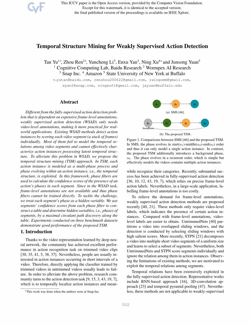
a1 a0 a2 a3

Background

a1 a2 a3

(a) SMS [46].

a1 a0 a2 a3

Background

a1 a2 a3

(b) The proposed TSM.

Figure 1. Comparisons between SMS [46] and the proposed TSM.

In SMS, the phase evolves in start(a1)-middle(a2)-end(a3) order

and thus it can only model a single action instance. In contrast,

the proposed TSM additionally introduces a background phase,

a0. The phase evolves in a recurrent order, which is simple but

effectively models the videos contains multiple action instances.

while recognize their categories. Recently, substantial suc-

cess has been achieved in fully-supervised action detection

[36, 10, 12, 43, 19, 7], which relies on precise frame-level

action labels. Nevertheless, in a large-scale application, la-

belling frame-level annotations is too costly.

To relieve the demand for frame-level annotations,

weakly supervised action detection methods are proposed

recently [40, 21]. These methods only require video-level

labels, which indicates the presence of certain action in-

stances. Compared with frame-level annotations, video-

level labels are easier to obtain. UntrimmedNets [40] par-

titions a video into overlapped sliding windows, and the

detection is conducted by selecting sliding windows with

high salient scores. More recently, STPN [21] decomposes

a video into multiple short video segments of a uniform size

and learns to select a subset of segments. Nevertheless, both

UntrimmedNets and STPN score segments individually and

ignore the relation among them in action instances. Observ-

ing the limitations of existing methods, we are motivated to

exploit the temporal relations among segments.

Temporal relations have been extensively exploited in

the fully-supervised action detection. Representative works

include RNN-based approach [16], 3D-convolution ap-

proach [23] and temporal pyramid pooling [47]. Neverthe-

less, these methods are not applicable to weakly-supervised

43215522

a1

a2

a3

a0

a0

a1

a2

a3

f1

f2

f3

f0

s1 sNsNs1

...

s1 sN

Loss

Segment Features

Scores Table

Phase Filters

Instance 1 Instance 2

-3

-1

-2

0 0 0 0 0 0 0 0 0 0 0 0 0 0 0 0 0 0 0 0 0 0

0 0 1 1 2 2 5 5 4 4 2 -2-2 1 0 3

4 6

1 31 4 3

0 3 2 １　0 1 1 0 0 -2-1 3 3 2 2 2

1 ４ 5 3 5 ６ 0 2 2 1 0 -1-2 2 1 2 4 4

(BG)

1 1 0

113

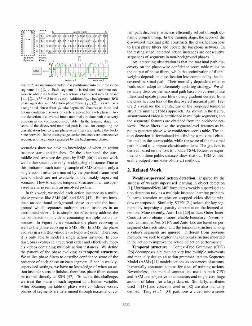
Figure 2. An untrimmed video V is partitioned into multiple video

segments {si}N

i=1. Each segment si is fed into backbone net-

work to obtain its feature. Each action is factorized into M phase

{am}Mm=1 (M = 3 in this case). Additionally, a background (BG)

phase a0 is devised. M action phase filters {fm}Mm=1 as well as a

background phase filter f0 take segments’ features as input and

obtain confidence scores of each segment for each phase. Ac-

tion detection is converted into a maximal circulant path discovery

problem in the confidence score table. In the training stage, the

score of the discovered maximal path is used for computing the

classification loss to learn phase-wise filters and update the back-

bone network. In the testing stage, action instances are consecutive

sequences of segments separated by the background phase.

scenarios since we have no knowledge of when an action

instance starts and finishes. On the other hand, the start-

middle-end structure designed by SMS [46] does not work

well either since it can only model a single instance. Due to

this limitation, each training sample of SMS contains only a

single action instance trimmed by the provided frame-level

labels, which are not available in the weakly-supervised

scenario. How to exploit temporal structure in an unsuper-

vised scenario remains an unsolved problem.

In this work, we model each action instance as a multi-

phase process like SMS [46] and SSN [47]. But we intro-

duce an additional background phase to model the back-

ground which separates multiple action instances in an

untrimmed video. It is simple but effectively address the

action detection in videos containing multiple action in-

stances. In Figure 1, we visualize the phase evolving as

well as the phase evolving in SMS [46]. In SMS, the phase

evolves in a start(a0)-middle (a1)-end(a2) order. Therefore,

it is only able to model a single action instance. In con-

trast, ours evolves in a recurrent order and effectively mod-

els videos containing multiple action instances. We define

the pattern of the phase evolving as temporal structure.

We utilize phase filters to describe confidence score of the

presence of each phase on each segment. Since in weakly-

supervised settings, we have no knowledge of when an ac-

tion instance starts or finishes, therefore, phase filters cannot

be trained directly as SSN [47]. To tackle this challenge,

we treat the phase of each segment as a hidden variable.

After obtaining the table of phase-wise confidence scores,

phases of segments are determined through maximal circu-

lant path discovery, which is efficiently solved through dy-

namic programming. In the training stage, the score of the

discovered maximal path constructs the classification loss

to learn phase filters and update the backbone network. In

the testing stage, detected action instances are consecutive

sequences of segments in non-background phases.

An interesting observation is that the maximal path dis-

covery on the phase-wise confidence score table relies on

the output of phase filters, while the optimization of filters’

weights depends on classification loss computed by the dis-

covered maximal path. Their mutually dependent relation

leads us to adopt an alternately updating strategy. We al-

ternately discover the maximal path based on current phase

filters and update phase filters using gradient derived from

the classification loss of the discovered maximal path. Fig-

ure 2 visualizes the architecture of the proposed temporal

structure mining (TSM) approach. As shown in the figure,

an untrimmed video is partitioned in multiple segments, and

the segments’ features are obtained from the backbone net-

work. Phase filters take the segment-level features as in-

put to generate phase-wise confidence scores table. The ac-

tion detection is formulated into finding a maximal circu-

lant path in the scores table, while the score of the maximal

path is used to compute classification loss. The gradient is

derived based on the loss to update TSM. Extensive exper-

iments on three public datasets show that our TSM consid-

erably outperforms state-of-the-art methods.

2. Related Work

Weakly-supervised action detection. Inspired by the

success of weakly supervised learning in object detection

[1], UntrimmedNets [40] formulates weakly supervised ac-

tion detection task as a multiple instance learning problem.

It learns attention weights on cropped video sliding win-

dow or proposals. Similarly, STPN [21] selects the key seg-

ments by imposing a sparsity constraint on the learned at-

tention. More recently, Auto-Loc [29] utilizes Outer-Inner-

Contrastive to obtain a more reliable boundary. Neverthe-

less, UntrimmedNet, STPN and Auto-Loc are based on per-

segment class activation and the temporal structure among

a video’s segments are ignored. Different from previous

methods, we seek to exploit the temporal structure inherited

in the action to improve the action detection performance.

Temporal structure. Context-Free Grammar (CFG)

[26] decomposes a human activity into multiple sub-events

and manually design an action grammar. Actom Sequence

Model (ASM) [11] models actions as sequences of actoms.

It manually annotates actoms for a set of training actions.

Nevertheless, the manual annotations used in both CFG

and ASM are subjective to annotators and might cost huge

amount of labors for a large dataset. Similarly, attributes

used in [18] and concepts used in [32] are also manually

defined. Tang et al. [34] partitions a video into a series

43225523

of events and designs a variable-duration hidden Markov

model (HMM) to model the events transitions. But the

huge amount of parameters of the designed HMM makes

the training difficult. Wang et al. [39] decompose an action

into atoms and phases. Clustering is used to discover ac-

tion atoms and continuous atoms are merged into AND/OR

structure phases. Nevertheless, it does not consider the case

when a video contains uninterested background. It might be

only applicable for action recognition on trimmed videos.

Structured Segment Network (SSN) [47] divides an action

instance into three stages and utilizes temporal pyramid

pooling to explicitly exploit temporal structure. Since in the

fully-supervised scenario, the start and end of an action in-

stance are known in training dataset, it is straightforward

to construct the temporal pyramid. Nevertheless, in the

weakly-supervised cases, no temporal annotations are pro-

vided, and thus we are not able to conduct temporal pyra-

mid pooling used in SSN. Structural Maximal Sum (SMS)

[46] also exploits the temporal structure in action instances.

SMS designs a start-middle-end structure, which can only

model a single action instance. In the training phase, due

to single instance limitation, SMS has to manually crop a

whole video into clips containing a single action instance

using the provided temporal annotations. Nevertheless, in

weakly-supervised scenarios, no temporal annotations are

provided, making the training of SMS infeasible. Mean-

while, some methods [2, 6, 25] align videos to transcripts.

They rely on temporal orderings of manually defined basic

actions. In contrast, ours only relies on video-level class

label and automatically discovers the action phases.

3. Problem Formulation

3.1. Definition

Given a video V , we uniformly decompose it into Nshort video segments [s1, · · · , sN ]. For each action class

c, we define M action phases {aj}Mj=1 and model each ac-

tion instance as a M -phase process. Meanwhile, the back-

ground is modelled by phase a0. We define xi = g(si,W)as the feature of segment si obtained from backbone where

W contains parameters of backbone. vjc,i is defined as the

confidence score of the presence of phase aj of class c in si:

vjc,i = f(xi,wjc, b

jc) = x⊤

i wjc + bjc, (1)

where f(·,wjc, b

jc) represents j-th action phase filter for the

class c. We use vjc,i to construct the confidence score table

visualized in Figure 3 where vjc,i is filled in the cell located

in row j and column i. We define (i, pi) as the cell in the

score table where the column index i is the segment index,

and the row index pi is the phase index, where pi ∈ [0,M ].We define [(1, p1), · · · , (N, pN )] as a path in the confidence

score table. For convenience, we omit the column index and

represent a path of class c by Pc = [p1, · · · , pN ].

3.2. Temporal Structure Mining

Now we describe the phase evolving constraint, which is

the core component of temporal structure modelling. Given

a segment si in the phase pi, the phase pi+1 of its next

segment si+1 only has two choices: 1) remaining the same

phase as si, 2) evolving to the next phase. Formally,

pi+1 ∈ {pi, (pi + 1)%(M + 1)}. (2)

The mod operation % means that the last phase aM evolves

to the background phase a0 and a0 evolves to the first action

phase a1. In other words, the action phase transits in a circu-

lant manner. This recurrent evolving mechanism effectively

handles videos containing multiple action instances.

Given an untrimmed video V , we obtain phase-wise con-

fidence scores of each segment {vjc,i}Mj=1 through Eq. (1) to

construct the confidence score table. Given a path Pc =[p1, p2, · · · , pN ] , we define the path score Fc(Pc) as

Fc(Pc) =

N∑

i=1

✶(pi 6= 0)vpi

c,i. (3)

where ✶(pi 6= 0) is the indicator function omitting segments

in background phase. Since the background’s scores are not

used in computing path score, by setting the background

score v0c,i = 0, we obtain an equivalent but simpler form as

Fc(Pc) =N∑

i=1

vpi

c,i. (4)

The temporal structure mining is formulated into discover-

ing a path constrained by Eq. (2) with maximal path score:

P∗c = argmax

Pc

Fc(Pc). (5)

We show an example of maximal circulant path in Fig-

ure 3 by green boxes. In the training stage, the score of

maximal circulant path Fc(P∗c ) represents the presence of

action c in the video, which constructs the classification

loss. In the testing stage, the action instances of a certain

class are detected by grouping consecutive segments sepa-

rated by background phase. As shown in Figure 3, it detects

two action instances, which are separated by background.

Until now, two problems remain unsolved: 1) how to

learn phase filters {f(·,wjc, b

jc)}

Mj=1 in Eq. (1); 2) how to

discover the maximal circulant path P∗c in Eq. (5) effi-

ciently. In Section 3.3 and 3.4, we tackle them, respectively.

3.3. Phase Filter Learning

Without frame-level action annotations, learning phase

filters is much more difficult than its fully-supervised coun-

terpart [47, 46]. We observe that filters learning relies on the

discovered maximal path, and on the same time the max-

imal path discovery depends on pre-trained phase filters.

43235524

-1.3 -2.0 0.3 0.4 0.6 0.2 0.1 0.1 0.0 -0.1 -0.5 0.3 0.2 0.2 0.1 -0.3

-2.1 -3.1 0.4 0.5 0.3 0.5 0.6 0.2 0.1 -0.2 -0.7 0.1 0.2 0.6 0.2 -0.2

-3.1 0.8 -0.3 0.1 0.1 0.2 0.2 0.5 0.2 -0.2 -0.3 -0.3 0.3 0.1 0.4 -0.3

0.0 0.0 0.0 0.0 0.0 0.0 0.0 0.0 0.0 0.0 0.0 0.0 0.0 0.0 0.0 0.0

a1

a2

a3

a0 (BG)

Instance 1 Instance 2

Figure 3. An example for confidence score table. The green bold

cells are along the maximal circulant path. Due to the phase evolv-

ing constraint, maximal path discovery is not equivalent to greed-

ily selecting the phase with highest score for each segment. For

instance, in the second column of the table, we select phase a0,

the background phase (background), even though phase a3 has the

largest confidence score in this column.

Algorithm 1 Alternately Updating

Input: Videos {Vk}Kk=1 and ground-truth labels {yk}

Kk=1.

Output: Weights of the phase filters {wjc, b

jc}

M,Cj=1,c=1,

backbone network weights W.

1: for c = 1 to C do

2: for j = 1 toM do

3: initialize wjc ,bjc

4: for k = 1 toK do

5: Vk → [sk,1, · · · , sk,N ]

6: for t = 1 to T do

7: for k = 1 toK do

8: xk,i ← g(sk,i,W)9: for c = 1 to C do

10: discover P∗k,c based on Algorithm 2

11: compute Lc based on Eq. (6)

12: for j = 1 toM do

13: compute ∂Lc

∂wjc

and ∂Lc

∂bjc

based on Eq. (7)

14: wjc ← wj

c − δ ∂Lc

∂wjc

, bjc ← bjc − δ ∂Lc

∂bjc

15: for i = 1 to N do

16: compute ∂Lc

∂xk,ibased on Eq. (8)

17: compute ∂Lc

∂Wuse Eq. (9)

18: W←W − δ ∂Lc

∂W

19: return {wjc}

M,Cj=1,c=1,W.

Their mutually dependence leads to the fact that the training

process can not be conducted in a sequential manner.

To tackle this problem, we adopt an alternately updat-

ing strategy consisting of two steps. In the first step, the

maximal path P∗c is discovered based on output of currently

phase filters {f(·,wjc, b

jc)}

Mj=1, using Maximal Path Dis-

covery as discussed in Sec. 3.4 (Algorithm 2). In the second

step, the path score of detected maximal path Fc(P∗c ) and

the video’s ground-truth class label yc ∈ {0, 1} are used to

compute the classification loss Lc defined as

Lc =− yc log(tanh(Fc(P∗c ) + ǫ)

− (1− yc) log(1− tanh(Fc(P∗c )).

(6)

Note that, Lc is not the standard cross-entropy loss. We

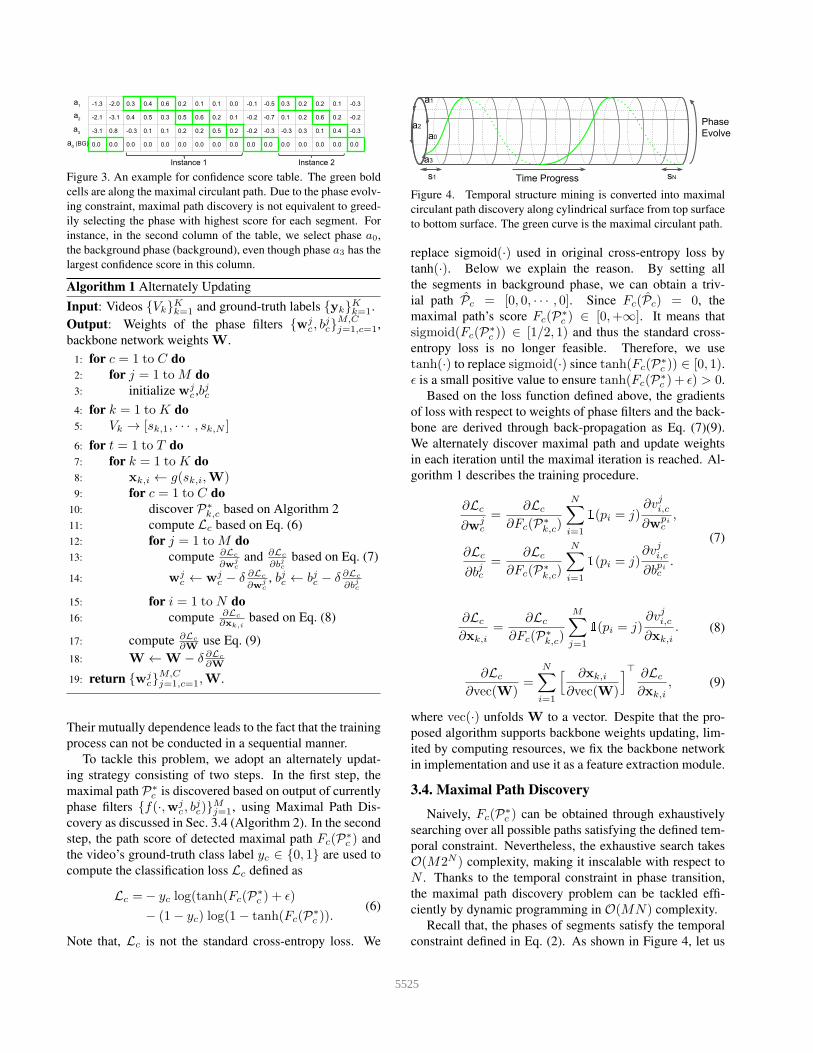
PhaseEvolve

Time Progresss1 sN

a0

a1

a2

a3

Figure 4. Temporal structure mining is converted into maximal

circulant path discovery along cylindrical surface from top surface

to bottom surface. The green curve is the maximal circulant path.

replace sigmoid(·) used in original cross-entropy loss by

tanh(·). Below we explain the reason. By setting all

the segments in background phase, we can obtain a triv-

ial path Pc = [0, 0, · · · , 0]. Since Fc(Pc) = 0, the

maximal path’s score Fc(P∗c ) ∈ [0,+∞]. It means that

sigmoid(Fc(P∗c )) ∈ [1/2, 1) and thus the standard cross-

entropy loss is no longer feasible. Therefore, we use

tanh(·) to replace sigmoid(·) since tanh(Fc(P∗c )) ∈ [0, 1).

ǫ is a small positive value to ensure tanh(Fc(P∗c ) + ǫ) > 0.

Based on the loss function defined above, the gradients

of loss with respect to weights of phase filters and the back-

bone are derived through back-propagation as Eq. (7)(9).

We alternately discover maximal path and update weights

in each iteration until the maximal iteration is reached. Al-

gorithm 1 describes the training procedure.

∂Lc

∂wjc

=∂Lc

∂Fc(P∗k,c)

N∑

i=1

✶(pi = j)∂vji,c∂wpi

c,

∂Lc

∂bjc=

∂Lc

∂Fc(P∗k,c)

N∑

i=1

✶(pi = j)∂vji,c∂bpi

c.

(7)

∂Lc

∂xk,i

=∂Lc

∂Fc(P∗k,c)

M∑

j=1

✶(pi = j)∂vji,c∂xk,i

. (8)

∂Lc

∂vec(W)=

N∑

i=1

[ ∂xk,i

∂vec(W)

]⊤ ∂Lc

∂xk,i

, (9)

where vec(·) unfolds W to a vector. Despite that the pro-

posed algorithm supports backbone weights updating, lim-

ited by computing resources, we fix the backbone network

in implementation and use it as a feature extraction module.

3.4. Maximal Path Discovery

Naively, Fc(P∗c ) can be obtained through exhaustively

searching over all possible paths satisfying the defined tem-

poral constraint. Nevertheless, the exhaustive search takes

O(M2N ) complexity, making it inscalable with respect to

N . Thanks to the temporal constraint in phase transition,

the maximal path discovery problem can be tackled effi-

ciently by dynamic programming in O(MN) complexity.

Recall that, the phases of segments satisfy the temporal

constraint defined in Eq. (2). As shown in Figure 4, let us

43245525

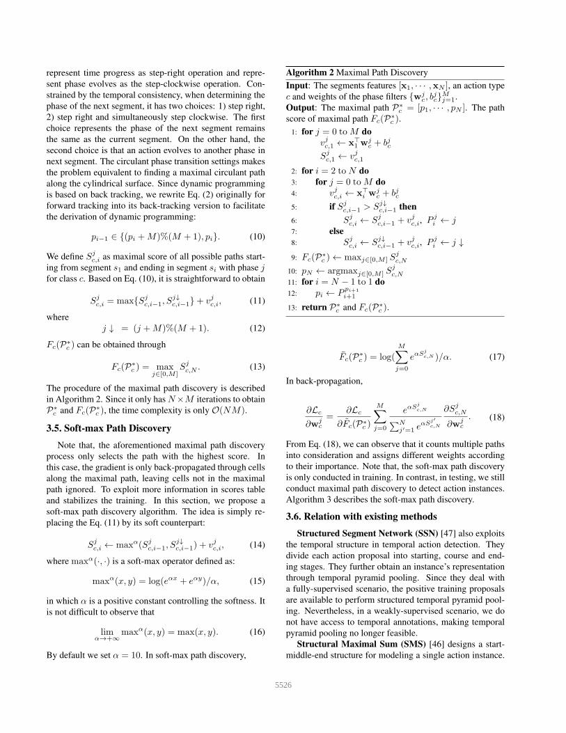
represent time progress as step-right operation and repre-

sent phase evolves as the step-clockwise operation. Con-

strained by the temporal consistency, when determining the

phase of the next segment, it has two choices: 1) step right,

2) step right and simultaneously step clockwise. The first

choice represents the phase of the next segment remains

the same as the current segment. On the other hand, the

second choice is that an action evolves to another phase in

next segment. The circulant phase transition settings makes

the problem equivalent to finding a maximal circulant path

along the cylindrical surface. Since dynamic programming

is based on back tracking, we rewrite Eq. (2) originally for

forward tracking into its back-tracking version to facilitate

the derivation of dynamic programming:

pi−1 ∈ {(pi +M)%(M + 1), pi}. (10)

We define Sjc,i as maximal score of all possible paths start-

ing from segment s1 and ending in segment si with phase jfor class c. Based on Eq. (10), it is straightforward to obtain

Sjc,i = max{Sj

c,i−1, Sj↓c,i−1}+ vjc,i, (11)

where

j ↓ = (j +M)%(M + 1). (12)

Fc(P∗c ) can be obtained through

Fc(P∗c ) = max

j∈[0,M ]Sjc,N . (13)

The procedure of the maximal path discovery is described

in Algorithm 2. Since it only has N×M iterations to obtain

P∗c and Fc(P

∗c ), the time complexity is only O(NM).

3.5. Soft­max Path Discovery

Note that, the aforementioned maximal path discovery

process only selects the path with the highest score. In

this case, the gradient is only back-propagated through cells

along the maximal path, leaving cells not in the maximal

path ignored. To exploit more information in scores table

and stabilizes the training. In this section, we propose a

soft-max path discovery algorithm. The idea is simply re-

placing the Eq. (11) by its soft counterpart:

Sjc,i ← maxα(Sj

c,i−1, Sj↓c,i−1) + vjc,i, (14)

where maxα(·, ·) is a soft-max operator defined as:

maxα(x, y) = log(eαx + eαy)/α, (15)

in which α is a positive constant controlling the softness. It

is not difficult to observe that

limα→+∞

maxα(x, y) = max(x, y). (16)

By default we set α = 10. In soft-max path discovery,

Algorithm 2 Maximal Path Discovery

Input: The segments features [x1, · · · ,xN ], an action type

c and weights of the phase filters {wjc, b

jc}

Mj=1.

Output: The maximal path P∗c = [p1, · · · , pN ]. The path

score of maximal path Fc(P∗c ).

1: for j = 0 toM do

vjc,1 ← x⊤1 w

jc + bjc

Sjc,1 ← vjc,1

2: for i = 2 to N do

3: for j = 0 toM do

4: vjc,i ← x⊤i w

jc + bjc

5: if Sjc,i−1 > Sj↓

c,i−1 then

6: Sjc,i ← Sj

c,i−1 + vjc,i, P ji ← j

7: else

8: Sjc,i ← Sj↓

c,i−1 + vjc,i, P ji ← j ↓

9: Fc(P∗c )← maxj∈[0,M ] S

jc,N

10: pN ← argmaxj∈[0,M ] Sjc,N

11: for i = N − 1 to 1 do

12: pi ← Ppi+1

i+1

13: return P∗c and Fc(P

∗c ).

Fc(P∗c ) = log(

M∑

j=0

eαSj

c,N )/α. (17)

In back-propagation,

∂Lc

∂wjc

=∂Lc

∂Fc(P∗c )

M∑

j=0

eαSj

c,N

∑Nj′=1 e

αSj′

c,N

∂Sjc,N

∂wjc

. (18)

From Eq. (18), we can observe that it counts multiple paths

into consideration and assigns different weights according

to their importance. Note that, the soft-max path discovery

is only conducted in training. In contrast, in testing, we still

conduct maximal path discovery to detect action instances.

Algorithm 3 describes the soft-max path discovery.

3.6. Relation with existing methods

Structured Segment Network (SSN) [47] also exploits

the temporal structure in temporal action detection. They

divide each action proposal into starting, course and end-

ing stages. They further obtain an instance’s representation

through temporal pyramid pooling. Since they deal with

a fully-supervised scenario, the positive training proposals

are available to perform structured temporal pyramid pool-

ing. Nevertheless, in a weakly-supervised scenario, we do

not have access to temporal annotations, making temporal

pyramid pooling no longer feasible.

Structural Maximal Sum (SMS) [46] designs a start-

middle-end structure for modeling a single action instance.

43255526

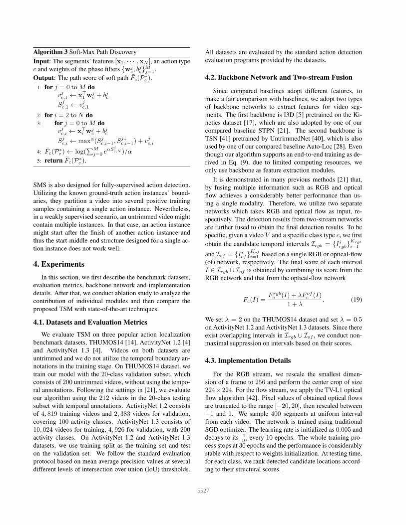
Algorithm 3 Soft-Max Path Discovery

Input: The segments’ features [x1, · · · ,xN ], an action type

c and weights of the phase filters {wjc, b

jc}

Mj=1.

Output: The path score of soft path Fc(P∗c ).

1: for j = 0 toM do

vjc,1 ← x⊤1 w

jc + bjc

Sjc,1 ← vjc,1

2: for i = 2 to N do

3: for j = 0 toM do

vjc,i ← x⊤i w

jc + bjc

Sjc,i ← maxα(Sj

c,i−1, Sj↓c,i−1) + vjc,i

4: Fc(P∗c )← log(

∑Mj=0 e

αSj

c,N )/α

5: return Fc(P∗c ).

SMS is also designed for fully-supervised action detection.

Utilizing the known ground-truth action instances’ bound-

aries, they partition a video into several positive training

samples containing a single action instance. Nevertheless,

in a weakly supervised scenario, an untrimmed video might

contain multiple instances. In that case, an action instance

might start after the finish of another action instance and

thus the start-middle-end structure designed for a single ac-

tion instance does not work well.

4. Experiments

In this section, we first describe the benchmark datasets,

evaluation metrics, backbone network and implementation

details. After that, we conduct ablation study to analyze the

contribution of individual modules and then compare the

proposed TSM with state-of-the-art techniques.

4.1. Datasets and Evaluation Metrics

We evaluate TSM on three popular action localization

benchmark datasets, THUMOS14 [14], ActivityNet 1.2 [4]

and ActivityNet 1.3 [4]. Videos on both datasets are

untrimmed and we do not utilize the temporal boundary an-

notations in the training stage. On THUMOS14 dataset, we

train our model with the 20-class validation subset, which

consists of 200 untrimmed videos, without using the tempo-

ral annotations. Following the settings in [21], we evaluate

our algorithm using the 212 videos in the 20-class testing

subset with temporal annotations. ActivityNet 1.2 consists

of 4, 819 training videos and 2, 383 videos for validation,

covering 100 activity classes. ActivityNet 1.3 consists of

10, 024 videos for training, 4, 926 for validation, with 200activity classes. On ActivityNet 1.2 and ActivityNet 1.3

datasets, we use training split as the training set and test

on the validation set. We follow the standard evaluation

protocol based on mean average precision values at several

different levels of intersection over union (IoU) thresholds.

All datasets are evaluated by the standard action detection

evaluation programs provided by the datasets.

4.2. Backbone Network and Two­stream Fusion

Since compared baselines adopt different features, to

make a fair comparison with baselines, we adopt two types

of backbone networks to extract features for video seg-

ments. The first backbone is I3D [5] pretrained on the Ki-

netics dataset [17], which are also adopted by one of our

compared baseline STPN [21]. The second backbone is

TSN [41] pretrained by UntrimmedNet [40], which is also

used by one of our compared baseline Auto-Loc [28]. Even

though our algorithm supports an end-to-end training as de-

rived in Eq. (9), due to limited computing resources, we

only use backbone as feature extraction modules.

It is demonstrated in many previous methods [21] that,

by fusing multiple information such as RGB and optical

flow achieves a considerably better performance than us-

ing a single modality. Therefore, we utilize two separate

networks which takes RGB and optical flow as input, re-

spectively. The detection results from two-stream networks

are further fused to obtain the final detection results. To be

specific, given a video V and a specific class type c, we first

obtain the candidate temporal intervals Irgb = {Iirgb}Krgb

i=1

and Iof = {Iiof}Kof

i=1 based on a single RGB or optical-flow

(of) network, respectively. The final score of each interval

I ∈ Irgb ∪ Iof is obtained by combining its score from the

RGB network and that from the optical-flow network

Fc(I) =F rgbc (I) + λF of

c (I)

1 + λ. (19)

We set λ = 2 on the THUMOS14 dataset and set λ = 0.5on ActivityNet 1.2 and ActivityNet 1.3 datasets. Since there

exist overlapping intervals in Irgb ∪ Iof , we conduct non-

maximal suppression on intervals based on their scores.

4.3. Implementation Details

For the RGB stream, we rescale the smallest dimen-

sion of a frame to 256 and perform the center crop of size

224×224. For the flow stream, we apply the TV-L1 optical

flow algorithm [42]. Pixel values of obtained optical flows

are truncated to the range [−20, 20], then rescaled between

−1 and 1. We sample 400 segments at uniform interval

from each video. The network is trained using traditional

SGD optimizer. The learning rate is initialized as 0.005 and

decays to its 110 every 10 epochs. The whole training pro-

cess stops at 30 epochs and the performance is considerably

stable with respect to weights initialization. At testing time,

for each class, we rank detected candidate locations accord-

ing to their structural scores.

43265527

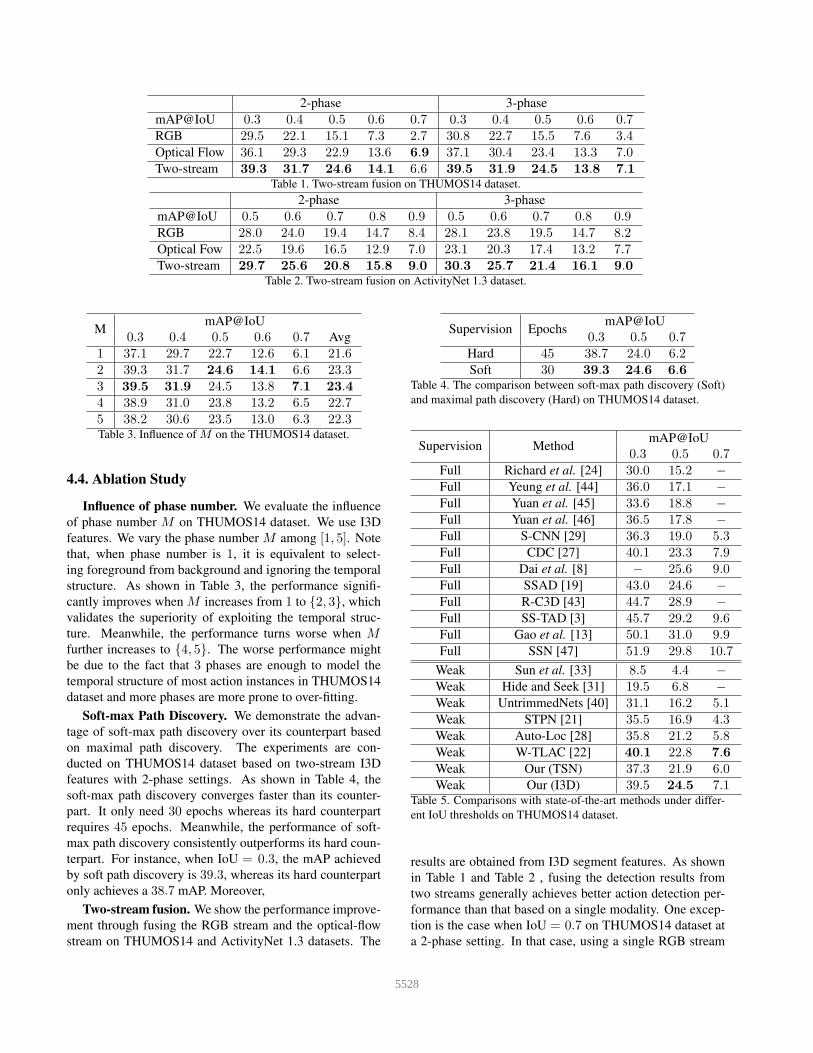
2-phase 3-phase

mAP@IoU 0.3 0.4 0.5 0.6 0.7 0.3 0.4 0.5 0.6 0.7RGB 29.5 22.1 15.1 7.3 2.7 30.8 22.7 15.5 7.6 3.4Optical Flow 36.1 29.3 22.9 13.6 6.9 37.1 30.4 23.4 13.3 7.0Two-stream 39.3 31.7 24.6 14.1 6.6 39.5 31.9 24.5 13.8 7.1

Table 1. Two-stream fusion on THUMOS14 dataset.

2-phase 3-phase

mAP@IoU 0.5 0.6 0.7 0.8 0.9 0.5 0.6 0.7 0.8 0.9RGB 28.0 24.0 19.4 14.7 8.4 28.1 23.8 19.5 14.7 8.2Optical Fow 22.5 19.6 16.5 12.9 7.0 23.1 20.3 17.4 13.2 7.7Two-stream 29.7 25.6 20.8 15.8 9.0 30.3 25.7 21.4 16.1 9.0

Table 2. Two-stream fusion on ActivityNet 1.3 dataset.

MmAP@IoU

0.3 0.4 0.5 0.6 0.7 Avg

1 37.1 29.7 22.7 12.6 6.1 21.62 39.3 31.7 24.6 14.1 6.6 23.33 39.5 31.9 24.5 13.8 7.1 23.44 38.9 31.0 23.8 13.2 6.5 22.75 38.2 30.6 23.5 13.0 6.3 22.3Table 3. Influence of M on the THUMOS14 dataset.

4.4. Ablation Study

Influence of phase number. We evaluate the influence

of phase number M on THUMOS14 dataset. We use I3D

features. We vary the phase number M among [1, 5]. Note

that, when phase number is 1, it is equivalent to select-

ing foreground from background and ignoring the temporal

structure. As shown in Table 3, the performance signifi-

cantly improves when M increases from 1 to {2, 3}, which

validates the superiority of exploiting the temporal struc-

ture. Meanwhile, the performance turns worse when Mfurther increases to {4, 5}. The worse performance might

be due to the fact that 3 phases are enough to model the

temporal structure of most action instances in THUMOS14

dataset and more phases are more prone to over-fitting.

Soft-max Path Discovery. We demonstrate the advan-

tage of soft-max path discovery over its counterpart based

on maximal path discovery. The experiments are con-

ducted on THUMOS14 dataset based on two-stream I3D

features with 2-phase settings. As shown in Table 4, the

soft-max path discovery converges faster than its counter-

part. It only need 30 epochs whereas its hard counterpart

requires 45 epochs. Meanwhile, the performance of soft-

max path discovery consistently outperforms its hard coun-

terpart. For instance, when IoU = 0.3, the mAP achieved

by soft path discovery is 39.3, whereas its hard counterpart

only achieves a 38.7 mAP. Moreover,

Two-stream fusion. We show the performance improve-

ment through fusing the RGB stream and the optical-flow

stream on THUMOS14 and ActivityNet 1.3 datasets. The

Supervision EpochsmAP@IoU

0.3 0.5 0.7Hard 45 38.7 24.0 6.2Soft 30 39.3 24.6 6.6

Table 4. The comparison between soft-max path discovery (Soft)

and maximal path discovery (Hard) on THUMOS14 dataset.

Supervision MethodmAP@IoU

0.3 0.5 0.7Full Richard et al. [24] 30.0 15.2 −Full Yeung et al. [44] 36.0 17.1 −Full Yuan et al. [45] 33.6 18.8 −Full Yuan et al. [46] 36.5 17.8 −Full S-CNN [29] 36.3 19.0 5.3Full CDC [27] 40.1 23.3 7.9Full Dai et al. [8] − 25.6 9.0Full SSAD [19] 43.0 24.6 −Full R-C3D [43] 44.7 28.9 −Full SS-TAD [3] 45.7 29.2 9.6Full Gao et al. [13] 50.1 31.0 9.9Full SSN [47] 51.9 29.8 10.7

Weak Sun et al. [33] 8.5 4.4 −Weak Hide and Seek [31] 19.5 6.8 −Weak UntrimmedNets [40] 31.1 16.2 5.1Weak STPN [21] 35.5 16.9 4.3Weak Auto-Loc [28] 35.8 21.2 5.8Weak W-TLAC [22] 40.1 22.8 7.6Weak Our (TSN) 37.3 21.9 6.0Weak Our (I3D) 39.5 24.5 7.1

Table 5. Comparisons with state-of-the-art methods under differ-

ent IoU thresholds on THUMOS14 dataset.

results are obtained from I3D segment features. As shown

in Table 1 and Table 2 , fusing the detection results from

two streams generally achieves better action detection per-

formance than that based on a single modality. One excep-

tion is the case when IoU = 0.7 on THUMOS14 dataset at

a 2-phase setting. In that case, using a single RGB stream

43275528

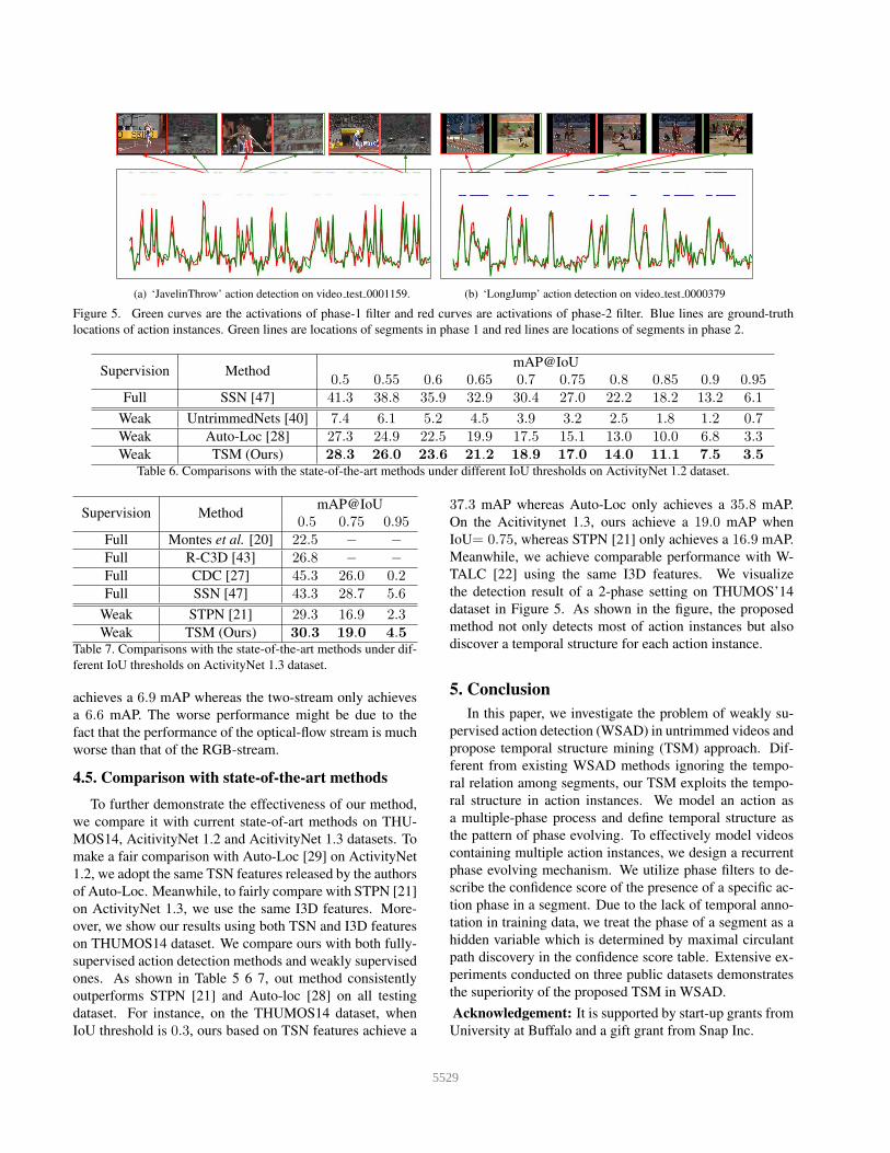
(a) ‘JavelinThrow’ action detection on video test 0001159. (b) ‘LongJump’ action detection on video test 0000379

Figure 5. Green curves are the activations of phase-1 filter and red curves are activations of phase-2 filter. Blue lines are ground-truth

locations of action instances. Green lines are locations of segments in phase 1 and red lines are locations of segments in phase 2.

Supervision MethodmAP@IoU

0.5 0.55 0.6 0.65 0.7 0.75 0.8 0.85 0.9 0.95Full SSN [47] 41.3 38.8 35.9 32.9 30.4 27.0 22.2 18.2 13.2 6.1

Weak UntrimmedNets [40] 7.4 6.1 5.2 4.5 3.9 3.2 2.5 1.8 1.2 0.7Weak Auto-Loc [28] 27.3 24.9 22.5 19.9 17.5 15.1 13.0 10.0 6.8 3.3Weak TSM (Ours) 28.3 26.0 23.6 21.2 18.9 17.0 14.0 11.1 7.5 3.5

Table 6. Comparisons with the state-of-the-art methods under different IoU thresholds on ActivityNet 1.2 dataset.

Supervision MethodmAP@IoU

0.5 0.75 0.95Full Montes et al. [20] 22.5 − −Full R-C3D [43] 26.8 − −Full CDC [27] 45.3 26.0 0.2Full SSN [47] 43.3 28.7 5.6

Weak STPN [21] 29.3 16.9 2.3Weak TSM (Ours) 30.3 19.0 4.5

Table 7. Comparisons with the state-of-the-art methods under dif-

ferent IoU thresholds on ActivityNet 1.3 dataset.

achieves a 6.9 mAP whereas the two-stream only achieves

a 6.6 mAP. The worse performance might be due to the

fact that the performance of the optical-flow stream is much

worse than that of the RGB-stream.

4.5. Comparison with state­of­the­art methods

To further demonstrate the effectiveness of our method,

we compare it with current state-of-art methods on THU-

MOS14, AcitivityNet 1.2 and AcitivityNet 1.3 datasets. To

make a fair comparison with Auto-Loc [29] on ActivityNet

1.2, we adopt the same TSN features released by the authors

of Auto-Loc. Meanwhile, to fairly compare with STPN [21]

on ActivityNet 1.3, we use the same I3D features. More-

over, we show our results using both TSN and I3D features

on THUMOS14 dataset. We compare ours with both fully-

supervised action detection methods and weakly supervised

ones. As shown in Table 5 6 7, out method consistently

outperforms STPN [21] and Auto-loc [28] on all testing

dataset. For instance, on the THUMOS14 dataset, when

IoU threshold is 0.3, ours based on TSN features achieve a

37.3 mAP whereas Auto-Loc only achieves a 35.8 mAP.

On the Acitivitynet 1.3, ours achieve a 19.0 mAP when

IoU= 0.75, whereas STPN [21] only achieves a 16.9 mAP.

Meanwhile, we achieve comparable performance with W-

TALC [22] using the same I3D features. We visualize

the detection result of a 2-phase setting on THUMOS’14

dataset in Figure 5. As shown in the figure, the proposed

method not only detects most of action instances but also

discover a temporal structure for each action instance.

5. Conclusion

In this paper, we investigate the problem of weakly su-

pervised action detection (WSAD) in untrimmed videos and

propose temporal structure mining (TSM) approach. Dif-

ferent from existing WSAD methods ignoring the tempo-

ral relation among segments, our TSM exploits the tempo-

ral structure in action instances. We model an action as

a multiple-phase process and define temporal structure as

the pattern of phase evolving. To effectively model videos

containing multiple action instances, we design a recurrent

phase evolving mechanism. We utilize phase filters to de-

scribe the confidence score of the presence of a specific ac-

tion phase in a segment. Due to the lack of temporal anno-

tation in training data, we treat the phase of a segment as a

hidden variable which is determined by maximal circulant

path discovery in the confidence score table. Extensive ex-

periments conducted on three public datasets demonstrates

the superiority of the proposed TSM in WSAD.

Acknowledgement: It is supported by start-up grants from

University at Buffalo and a gift grant from Snap Inc.

43285529

References

[1] Hakan Bilen and Andrea Vedaldi. Weakly supervised deep

detection networks. In CVPR, 2016.

[2] Piotr Bojanowski, Remi Lajugie, Francis Bach, Ivan Laptev,

Jean Ponce, Cordelia Schmid, and Josef Sivic. Weakly su-

pervised action labeling in videos under ordering constraints.

In ECCV, 2014.

[3] S Buch, V Escorcia, B Ghanem, L Fei-Fei, and JC

Niebles. End-to-end, single-stream temporal action detec-

tion in untrimmed videos. In BMVC, 2017.

[4] Fabian Caba Heilbron, Victor Escorcia, Bernard Ghanem,

and Juan Carlos Niebles. Activitynet: A large-scale video

benchmark for human activity understanding. In CVPR,

2015.

[5] Joao Carreira and Andrew Zisserman. Quo vadis, action

recognition? a new model and the kinetics dataset. In CVPR,

pages 4724–4733, 2017.

[6] Chien-Yi Chang, De-An Huang, Yanan Sui, Li Fei-Fei, and

Juan Carlos Niebles. D3tw: Discriminative differentiable

dynamic time warping for weakly supervised action align-

ment and segmentation. CoRR, abs/1901.02598, 2019.

[7] Yu-Wei Chao, Sudheendra Vijayanarasimhan, Bryan Sey-

bold, David A Ross, Jia Deng, and Rahul Sukthankar. Re-

thinking the faster R-CNN architecture for temporal action

localization. In CVPR, 2018.

[8] Xiyang Dai, Bharat Singh, Guyue Zhang, Larry S Davis, and

Yan Qiu Chen. Temporal context network for activity local-

ization in videos. In ICCV, 2017.

[9] Achal Dave, Olga Russakovsky, and Deva Ramanan. Predic-

tivecorrective networks for action detection. In CVPR, 2017.

[10] Tran Du, Yuan Junsong, and David Forsyth. Video event de-

tection: From subvolume localization to spatiotemporal path

search. IEEE Transactions on Pattern Analysis and Machine

Intelligence, 36(2):404–416, 2013.

[11] Adrien Gaidon, Zaid Harchaoui, and Cordelia Schmid. Ac-

tom sequence models for efficient action detection. In CVPR

2011, pages 3201–3208. IEEE, 2011.

[12] Yu Gang and Junsong Yuan. Fast action proposals for human

action detection and search. In CVPR, 2015.

[13] Jiyang Gao, Zhenheng Yang, and Ram Nevatia. Cas-

caded boundary regression for temporal action detection. In

BMVC, 2017.

[14] A Gorban, H Idrees, YG Jiang, A Roshan Zamir, I Laptev, M

Shah, and R Sukthankar. Thumos challenge: Action recog-

nition with a large number of classes, 2015.

[15] Fabian Caba Heilbron, Wayner Barrios, Victor Escorcia, and

Bernard Ghanem. Scc: Semantic context cascade for effi-

cient action detection. In CVPR, 2017.

[16] Rui Hou, Rahul Sukthankar, and Mubarak Shah. Real-time

temporal action localization in untrimmed videos by sub-

action discovery. In BMVC, 2017.

[17] Will Kay, Joao Carreira, Karen Simonyan, Brian Zhang,

Chloe Hillier, Sudheendra Vijayanarasimhan, Fabio Viola,

Tim Green, Trevor Back, Paul Natsev, et al. The kinetics hu-

man action video dataset. arXiv preprint arXiv:1705.06950,

2017.

[18] Weixin Li and Nuno Vasconcelos. Recognizing activities by

attribute dynamics. NIPS, 2013.

[19] Tianwei Lin, Xu Zhao, and Zheng Shou. Single shot tempo-

ral action detection. In ACM on Multimedia, 2017.

[20] Alberto Montes, Amaia Salvador, Santiago Pascual, and

Xavier Giro-i Nieto. Temporal activity detection in

untrimmed videos with recurrent neural networks. arXiv

preprint arXiv:1608.08128, 2016.

[21] Phuc Nguyen, Ting Liu, Gautam Prasad, and Bohyung Han.

Weakly supervised action localization by sparse temporal

pooling network. In CVPR, 2018.

[22] Sujoy Paul, Sourya Roy, and Amit K Roy-Chowdhury. W-

talc: Weakly-supervised temporal activity localization and

classification. In ECCV, 2018.

[23] Colin Lea Michael D Flynn Rene and Vidal Austin Reiter

Gregory D Hager. Temporal convolutional networks for ac-

tion segmentation and detection. In ICCV, 2017.

[24] Alexander Richard, Hilde Kuehne, and Juergen Gall. Weakly

supervised action learning with RNN based fine-to-coarse

modeling. In CVPR, pages 1273–1282, 2017.

[25] Alexander Richard, Hilde Kuehne, Ahsan Iqbal, and Juer-

gen Gall. Neuralnetwork-viterbi: A framework for weakly

supervised video learning. In ECCV, 2018.

[26] Michael S Ryoo and Jake K Aggarwal. Semantic represen-

tation and recognition of continued and recursive human ac-

tivities. IJCV, 82(1), 2009.

[27] Zheng Shou, Jonathan Chan, Alireza Zareian, Kazuyuki

Miyazawa, and Shih-Fu Chang. Cdc: Convolutional-de-

convolutional networks for precise temporal action localiza-

tion in untrimmed videos. In CVPR, pages 1417–1426, 2017.

[28] Zheng Shou, Hang Gao, Lei Zhang, Kazuyuki Miyazawa,

and Shih-Fu Chang. Autoloc: Weakly-supervised temporal

action localization in untrimmed videos. In ECCV, pages

154–171, 2018.

[29] Zheng Shou, Dongang Wang, and Shih-Fu Chang. Temporal

action localization in untrimmed videos via multi-stage cnns.

In CVPR, 2016.

[30] Karen Simonyan and Andrew Zisserman. Two-stream con-

volutional networks for action recognition in videos. In

NIPS, 2014.

[31] Krishna Kumar Singh and Yong Jae Lee. Hide-and-seek:

Forcing a network to be meticulous for weakly-supervised

object and action localization. In ICCV, 2017.

[32] Chen Sun and Ram Nevatia. Active: Activity concept tran-

sitions in video event classification. In ICCV, 2013.

[33] Chen Sun, Sanketh Shetty, Rahul Sukthankar, and Ram

Nevatia. Temporal localization of fine-grained actions in

videos by domain transfer from web images. In ACM on

Multimedia, 2015.

[34] Kevin Tang, Li Fei-Fei, and Daphne Koller. Learning latent

temporal structure for complex event detection. In CVPR,

2012.

[35] Du Tran, Lubomir Bourdev, Rob Fergus, Lorenzo Torresani,

and Manohar Paluri. Learning spatiotemporal features with

3d convolutional networks. In ICCV, 2015.

[36] Du Tran and Junsong Yuan. Max-margin structured output

regression for spatio-temporal action localization. In NIPS,

2012.

43295530

[37] Zhigang Tu, Hongyan Li, Dejun Zhang, Justin Dauwels,

and Junsong Yuan. Action-stage emphasized spatio-temporal

vlad for video action recognition. IEEE Transactions on Im-

age Processing, 28(6):2799–2812, 2019.

[38] Zhigang Tu, Xie Wei, Qianqing Qin, Ronald Poppe,

Remco C. Veltkamp, Baoxin Li, and Junsong Yuan. Multi-

stream cnn: Learning representations based on human-

related regions for action recognition. Pattern Recognition,

79:32–43, 2018.

[39] Limin Wang, Yu Qiao, and Xiaoou Tang. Mining motion

atoms and phrases for complex action recognition. In ICCV,

2013.

[40] Limin Wang, Yuanjun Xiong, Dahua Lin, and Luc Van Gool.

Untrimmednets for weakly supervised action recognition

and detection. In CVPR, 2017.

[41] Limin Wang, Yuanjun Xiong, Zhe Wang, Yu Qiao, Dahua

Lin, Xiaoou Tang, and Luc Van Gool. Temporal segment

networks: Towards good practices for deep action recogni-

tion. In ECCV, 2016.

[42] Andreas Wedel, Thomas Pock, Christopher Zach, Horst

Bischof, and Daniel Cremers. An improved algorithm for

tv-l 1 optical flow. In Statistical and geometrical approaches

to visual motion analysis. Springer, 2009.

[43] Huijuan Xu, Abir Das, and Kate Saenko. R-C3D: region

convolutional 3D network for temporal activity detection. In

ICCV, pages 5794–5803, 2017.

[44] Serena Yeung, Olga Russakovsky, Greg Mori, and Li Fei-

Fei. End-to-end learning of action detection from frame

glimpses in videos. In CVPR, 2016.

[45] Jun Yuan, Bingbing Ni, Xiaokang Yang, and Ashraf A Kas-

sim. Temporal action localization with pyramid of score dis-

tribution features. In CVPR, 2016.

[46] Ze-Huan Yuan, Jonathan C Stroud, Tong Lu, and Jia Deng.

Temporal action localization by structured maximal sums. In

CVPR, 2017.

[47] Yue Zhao, Yuanjun Xiong, Limin Wang, Zhirong Wu, Xi-

aoou Tang, and Dahua Lin. Temporal action detection with

structured segment networks. In ICCV, 2017.

43305531