Temporal and Spatial Variation in Switchgrass Biomass Composition and Theoretical Ethanol Yield

54 Agronomy Journa l • Volume104 , I s sue1 • 2012

Biofuels

TemporalandSpatialVariationinSwitchgrassBiomassCompositionandTheoreticalEthanolYield

M.R.Schmer,*K.P.Vogel,R.B.Mitchell,B.S.Dien,H.G.Jung,andM.D.Casler

Published in Agron. J. 104:54–64 (2012)Posted online 23 Nov 2011doi:10.2134/agronj2011.0195Copyright © 2012 by the American Society of Agronomy, 5585 Guilford Road, Madison, WI 53711. All rights reserved. No part of this periodical may be reproduced or transmitted in any form or by any means, electronic or mechanical, including photocopying, recording, or any information storage and retrieval system, without permission in writing from the publisher.

Cellulosic refineries will require substan-tial amounts of biomass on a year-round basis and are

expected to have higher capital costs than similar sized grain ethanol plants based on first-generation biomass refining technology (Wright and Brown, 2007). A reliable feedstock supply will be essential in maintaining stable operational costs. Further, cellulosic refineries will be required to convert biomass with potentially greater feedstock quality variability than existing corn (Zea mays L.) grain ethanol plants. Switchgrass is being developed as a biomass energy crop for the temper-ate regions of North America (Vogel and Mitchell, 2008). Temporal and spatial variation information across production years and fields for biomass yield and quality will be needed for establishing reliable feedstock supply areas for a cellulosic biorefinery. Information on field-scale spatial and temporal variation for biomass yield of switchgrass is becoming available (Schmer et al., 2010). Switchgrass biomass composition and theoretical ethanol production at the field-scale have thus far not been reported.

Biomass conversion to transportation fuels by biochemical methods will be dependent on efficient cellulose and hemicel-lulose polymer hydrolysis to simple sugars and then conver-sion to oxygenated hydrocarbons (Himmel et al., 2007). First generation cellulosic biorefineries, using biochemical methods, will produce primarily ethanol by converting cellulose, hemicel-lulose, and noncell wall carbohydrates into simple sugars which are then fermented to ethanol by genetically engineered organ-isms (Lynd et al., 1991; Perlack et al., 2005). Lignin, an abun-dant phenolic polymer in cell walls, can be used for combined heat and power generation (Demirbas, 2001; Lynd and Wang, 2003; Sheehan et al., 2003). Biochemical methods involve a pre-treatment to reduce cell wall recalcitrance and increase cell wall porosity, a saccharification process to hydrolyze complex poly-saccharides to monosaccharides, and a fermentation process to convert monosaccharides to a biofuel (Stephanopoulos, 2007). Near-term commercialized efforts to convert lignocellulosic feedstocks to biofuels through biochemical methods will likely involve simultaneous saccharification and fermentation (SSF). Alternative conversion systems such as consolidated bioprocess-ing which combines the enzymatic production, hydrolysis, and fermentation process into one reactor, thus reducing capital costs and increasing biorefinery efficiency, are expected to be commercially available as well (Lynd et al., 2005).

Cellulosic biomass conversion to biofuels via biochemi-cal or thermochemical methods require more complex and

ABstrActInformation on temporal and spatial variation in switchgrass (Panicum virgatum L.) biomass composition as it affects ethanol yield (L Mg–1) at a biorefinery and ethanol production (L ha–1) at the field-scale has previously not been available. Switchgrass biomass samples were collected from a regional, on-farm trial and biomass composition was determined using newly developed near-infrared reflectance spectroscopy (NIRS) prediction equations and theoretical ethanol yield (100% conversion efficiency) was calculated. Total hexose (cell wall polysaccharides and soluble sugars) concentration ranged from 342 to 398 g kg–1 while pentose (arabinose and xylose) concentration ranged from 216 to 245 g kg–1 across fields. Theoretical ethanol yield varied sig-nificantly by year and field, with 5 yr means ranging from 381 to 430 L Mg–1. Total theoretical ethanol production ranged from 1749 to 3691 L ha–1 across fields. Variability (coefficient of variation) within established switchgrass fields ranged from 1 to 4% for theoretical ethanol yield (L Mg–1) and 14 to 38% for theoretical ethanol production (L ha–1). Most fields showed a lack of spatial consistency across harvest years for theoretical ethanol yield or total theoretical ethanol production. Switchgrass biomass composition from farmer fields can be expected to have significant annual and field-to-field variation in a production region, and this variation will significantly affect ethanol or other liquid fuel yields per ton or hectare. Cellulosic biorefineries will need to consider this potential variation in biofuel yields when developing their business plans.

M.R. Schmer, USDA-ARS, Agroecosystem Management Research Unit, Lincoln, NE 68586-0937; K.P. Vogel and R.B. Mitchell, USDA-ARS, Grain, Forage, and Bioenergy Research Unit, Lincoln, NE 68586-0937; B.S. Dien, USDA-ARS, Bioenergy Research Unit, Rm. 3300, 1815 N. University St., Peoria, IL 61604-3999; H.G. Jung, USDA-ARS, Plant Science Research Unit, St. Paul, MN 55108-6026; M.D. Casler, USDA-ARS, U.S. Dairy Forage Research Center, Madison, WI 53706. Received 20 June 2011. *Corresponding author ([email protected]).

Abbreviations: ARA, arabinose; CRP, Conservation Reserve Program; ETOHTLT, total theoretical ethanol yield from all biomass sugars; FRU, fructose; GAL, galactose; GLC, cell wall glucose; GLCS, soluble glucose; HEX, total hexose; HEXEL, theoretical ethanol yield from all biomass hexoses; MAN, mannose; NIRS, near-infrared reflectance spectroscopy; NSC, nonstructural carbohydrates; PENTETL, theoretical ethanol yield from pentose sugars; PDSI, Palmer drought severity index; SSF, simultaneous saccharification and fermentation; STA, starch; SUC, sucrose; XYL, cell wall xylose.

Agronomy Journa l • Volume104, Issue1 • 2012 55

comprehensive analyses of feedstock composition determina-tions than typical forage quality analyses (Dien, 2010; Dien et al., 2006; Dowe and McMillan, 2001). Estimated costs of feed-stock composition analyses using wet laboratory methods are approximately $300 per sample without including equipment or laboratory overhead costs (Vogel et al., 2011). Near-infrared reflectance spectroscopy is a nondestructive technology that can be used to obtain rapid, low-cost, high-throughput and accurate estimates of agricultural product composition if suit-able prediction equations are available. The NIRS technology has been widely used in the food and pharmaceutical sector including recent advances to accurately predict corn grain quality and total fermentable carbohydrate content at dry-grind ethanol plants (Bothast and Schlicher, 2005). Advances in NIRS technology have made it feasible and analytically acceptable to determine if predicted spectral profile samples are within the spectral profile of the calibration set without con-tinual wet laboratory verification (Murray and Cowe, 2004; Shenk and Westerhaus, 1991; Westerhaus et al., 2004). This study was made feasible by USDA-ARS development of NIRS calibrations for switchgrass biomass composition including cell wall and soluble sugars which enables hundreds of biomass samples to be economically evaluated for biomass composition (Vogel et al., 2011). These NIRS calibrations are being made available for use by other laboratories, both public and private, through the NIRS Consortium (http://nirsconsortium.org/default.aspx; verified 18 Nov. 2011).

Cell wall and soluble carbohydrate biomass composition estimates at the field-scale for multiple years across a diverse geographical region have not been previously reported for switchgrass. The effect of variation in biomass composition on potential ethanol yield via SSF (L mg–1) and ethanol pro-duction per unit area (L ha–1) over years and fields in a large potential production region have likewise not been previously reported. Primary objectives of this study were to quantify temporal and spatial variation in biomass composition that can occur in switchgrass biomass over years and fields in a produc-tion region and to determine the effects of this variation on theoretical ethanol yield (L Mg–1) and production (L ha–1).

MAteriAls And MethodsThe study was conducted on farm fields in North Dakota

(two fields), South Dakota (four fields), and Nebraska (four fields) as a component of a large-scale, multipurpose experi-ment which included studies on switchgrass establishment, economics, yield modeling, net energy calculations, soil carbon sequestration, and spatial and temporal biomass yield variation (Kiniry et al., 2008; Liebig et al., 2008; Perrin et al., 2008; Schmer et al., 2006, 2008, 2010). Detailed information on switchgrass biomass production for each farm can be found in the previous reports cited above. Farms are identified by the nearest town (Fig. 1). The 10 fields were located in a major agro-ecoregion where previous economic model analyses indicated switchgrass grown as a biomass energy crop would be economi-cally feasible (Walsh, 1998). Fields were chosen based on char-acteristics of the region and qualifications in the Conservation Reserve Program (CRP). Nebraska fields were planted in 2000. The Atkinson, NE, field was replanted in 2001 because of stand failure caused by drought. The South Dakota and North

Dakota fields were planted in 2001. Field size ranged from 3 to 9.5 ha with an average of 6.7 ha. Farm cooperators man-aged all aspects of switchgrass production and harvest using a set of recommended management practices based on previous small plot research which included fertilization and harvesting procedures (Vogel, 2004).

Cultivars selected for each field were based on prior research within respective geographical regions. Switchgrass cultivars used in the study were ‘Cave-in-Rock’, ‘Trailblazer’, ‘Shaw-nee’, and ‘Sunburst’. The selected cultivars were primarily developed for use in livestock pastures. Soil descriptions, previous cropping history and field size by location have been described previously (Liebig et al., 2008; Schmer et al., 2006). Nitrogen fertilization rates were based on previous research in the Central Plains which showed that at current switchgrass yield levels, approximately 10 to 12 kg N ha–1 is required for each Mg ha–1 of expected biomass yield (Vogel et al., 2002). Nitrogen application varied across sites based on biomass yield expectations. Over the 5 yr period of the switchgrass stands, site averages of applied N ranged from 31 to 104 kg N ha–1 yr–1 (mean = 74 kg N ha–1) (Schmer et al., 2010).

Fields were mechanically harvested and baled by cooperators. Based on previous research, optimal harvest times are when switchgrass is at anthesis which occurs in early to mid-August in the Great Plains or after a killing frost (Parrish and Fike, 2005; Vogel et al., 2002). Most cooperators chose to harvest at emerged inflorescence to postanthesis (early to mid-August) in postestablishment years, except for the Bristol and Munich fields, which were harvested after a killing frost. Six fields were mechanically harvested in the establishment year while

Fig. 1. location of switchgrass fields managed for bioenergy in the Great Plains region.

56 Agronomy Journa l • Volume104, Issue1 • 2012

the Lawrence, Crofton, and Douglas fields were burned the following spring. The establishment year biomass at Ethan was neither removed nor burned the following spring but rather left standing due to lodging and subsequent switchgrass early spring growth in 2002.

Before mechanical harvest, fields were sampled each year at multiple quadrat sites to determine within-field variation for biomass yield and composition. Quadrat sample sites were randomly chosen by stratification based on cultivar and/or topography within each field (Schmer et al., 2010). A 12-chan-nel global position system receiver (Lowrance Globalmap 1001; Catoosa, OK1) was used to georeference each quadrat site within each switchgrass field. Biomass yields were estimated at 16 quadrat sites within a field using a 1- by 1-m quadrat in 2000 and a 0.3- by 3.66-m frame (1.1 m2) in 2001 through 2005 at the plant maturity stage of R1 to R5 (panicle fully emerged from boot to postanthesis) except for the establish-ment year which were sampled after a killing frost (Moore et al., 1991). Total plant biomass within the frame was clipped to a 10-cm stubble height and weighed with a portable electronic scale (Intercomp CS750, Minneapolis, MN). A subsample was dried at 55°C until a constant weight was reached to determine dry matter yield.

Switchgrass biomass subsamples from each sample site were ground through a 2-mm screen in a Wiley mill and then reground in a cyclone-type mill (Udy Corp., Ft. Collins CO) to pass a 1-mm screen. Ground samples were scanned using a Model 6500 near-infrared spectrometer (NIRSystems, Silver Springs, MD; now FOSS NIRSystems, Inc., Laurel, MD). A comprehensive set of switchgrass NIRS prediction equa-tions were used to predict the composition of the harvested biomass samples (Vogel et al., 2011). The calibration equa-tions were based on a set of switchgrass samples selected from several thousand switchgrass samples in a two-tiered process which represented a wide range of plant maturities, cultivars, ecotypes, fertility rates, and environments (Vogel et al., 2011). The NIRS calibration set of samples (n = 112) was analyzed for chemical composition, ethanol and pentose sugar yields following pretreatment, and SSF using commercial cellulases and Saccharomyces cerevisiae, and forage quality traits using wet laboratory methods (Dien et al., 2006; Vogel et al., 2011). The results of the wet laboratory analyses were then used to develop the NIRS prediction equations with specific calibration statistics reported between the wet laboratory value and NIRS predicted value (Vogel et al., 2011). No samples from this study were used in the development of the NIRS calibrations. Sample fitness from this study was determined using the Global H statistic (Murray and Cowe, 2004). The Global H statistic (Mahalanobis distance) is used to compare spectral profile of calibration samples and the samples to be analyzed. Samples with Global H values greater than three were excluded from the analysis (<4% of total samples). The NIRS calibrations are considered valid in estimating composition when Global H statistic values from analyzed samples are three or less (Murray and Cowe, 2004; Shenk and Westerhaus, 1991).

Although the available NIRS prediction equations can esti-mate 20 compositional components and 13 complex feedstock traits (Vogel et al., 2011), the focus in this report will be on the major biomass sugars that can be converted into ethanol and Klason lignin concentration. These carbohydrate traits include cell wall glucose (GLC), cell wall xylose (XYL), total hexose (HEX) which includes cell wall hexoses (GLC, mannose [MAN], galactose [GAL]) and nonstructural carbohydrates (NSC) of the biomass. The NSC consists of the soluble carbo-hydrates (glucose [GLCS], sucrose [SUC], and fructose [FRU]) and starch (STA) present in switchgrass biomass.

Total hexoses were calculated as per Vogel et al. (2011) as follows:

1. HEX (g kg–1) = [(MAN + GAL + GLC)(180/162)]+ NSC, where NSC is:

2. NSC (g kg–1) = GLCS + FRU + SUC + STA.

Total pentose includes XYL and arabinose (ARA).Theoretical ethanol yield and ethanol production was calcu-

lated using the following equations (Vogel et al., 2011):

3. Theoretical ethanol yield from all biomass hexoses: HEXEL (L Mg–1) = {[(MAN + GAL + GLC + STA) × 0.57] + [(GLCS + FRU) × 0.51) + (SUC × 0.537)] × 1.267}; assuming 100% conversion.

4. Theoretical ethanol yield from pentose sugars: PENTETL (L Mg–1) = (ARA + XYL) × 0.579 × 1.267.

5. Total Theoretical ethanol yield from all biomass sugars: ETOHTLT (L Mg–1) = HEXEL + PENTETL.

6. Total theoretical ethanol production (L ha–1) = ETOHTLT × biomass production yield (Mg ha–1).

Theoretical ethanol production values (L ha–1) for each sample site by field, harvest, and year were calculated based on quadrat yields and the composition of the biomass sample from each quadrat using the procedures described above.

statistical Analysis

The study was analyzed as a repeated-measure experiment, by field, with stand age (establishment year through Year 5) as a fixed effect while calendar year (2000 through 2005) was treated as a random effect to differentiate between the normal stand maturation trend over time and random weather effects (Loughin, 2006). Data were analyzed by cultivar and harvest year for Crofton, Douglas, and Lawrence where different cul-tivars were planted in the same field. Data were analyzed using the mixed procedure in SAS (Littel et al., 1996). Main effects and any interactions were considered significant when P £ 0.05. Mean separations was performed using Fisher’s LSD.

Pearson correlations were calculated among the cell wall composition traits. Variability in theoretical ethanol yield and theoretical ethanol production were determined using coefficient of variation by field and established harvest years (harvest years three through five). Spearman rank correlations were used to quantify year-to-year spatial consistency for theoretical ethanol yield (L Mg–1) and theoretical ethanol production (L ha–1) within a field. Rank correlations were based on the ranking of the sample sites within a field for all harvest years. Spearman rank

1 Trade and company names or commercial products mentioned is solely for the purpose of providing specific information and does not imply recommendation of endorsement by the U.S. Department of Agriculture.


correlations as suggested by Florin et al. (2009) above r = 0.5 would indicate that spatial patterns exist for sample sites within a field over harvest years while correlations below r = 0.5 would indicate a lack of spatial pattern consistency over harvest years.

resultsMean annual precipitation for the fields sites during the 5

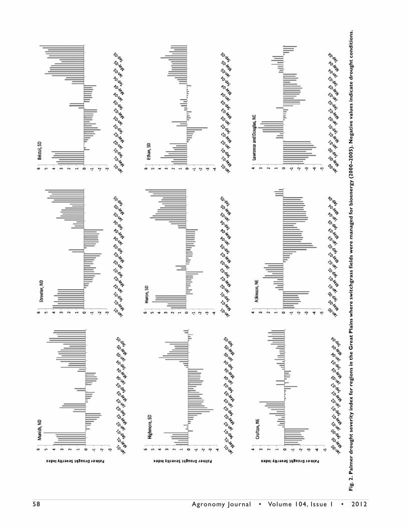
yr of study ranged from 430 mm in the west to 779 mm in the east, while mean annual temperature ranges from 2.7°C in the north to 12.8°C in the south (Schmer et al., 2010). Drought conditions were prevalent at most fields for the study duration as indicated by the Palmer drought severity index (PDSI) (Fig. 2). Negative PDSI values indicate degree of drought severity. Switchgrass fields in North Dakota and South Dakota tended to have above average precipitation conditions at establishment phase and at the end of the study (Fig. 2). Switchgrass fields in

Nebraska were under moderate drought conditions during the establishment phase with above average precipitation in 2001 (Fig. 2). Drought conditions were more prevalent at the south-ern and western fields (Fig. 1 and 2).

Total hexose components differed by harvest year for all fields (Table 1). Hexose sugars ranged from 342 g kg–1 at Munich to 398 g kg–1 at Lawrence across fields (Tables 2 and 3). Hexose concentrations differed by cultivar at Douglas and Lawrence (Table 1) with Cave-in-Rock and Shawnee hav-ing higher hexose concentrations than Trailblazer (Table 3). Pentose concentrations differed across harvest years at all fields with average concentrations ranging from 216 g kg–1 at Munich to 245 g kg–1 at Crofton. Cell wall glucose, found primarily in cellulose, comprised 66 to 82% of the total switch-grass hexose concentration while XYL was the most abundant pentose carbohydrate, found in hemicellulose, comprising 77

table 1. Analysis of variance F values and statistical significance for estimated switchgrass biofuel quality parameters from fields managed for bioenergy.

interaction

Field locations

Munich streeter Bristol highmore huron ethan Atkinson crofton douglas lawrence

Totalhexose,gkg–1

Harvestyear(HY) 81.6*** 28.8*** 38.4*** 102.9*** 119.0*** 4.63*** 112.2*** 34.9*** 9.6*** 34.8***

Cultivar(C) 0.75 6.8* 11.9***

HYĆ 0.26 1.6 1.7

Glucose,gkg–1

HY 147.7*** 34.4*** 89.5*** 112.7*** 86.7*** 1.65 36.7*** 25.4*** 8.61*** 102.6***

C 7.10*** 23.3*** 26.6***

HYĆ 0.9 0.6 3.4*

Pentose,gkg–1

HY 83.6*** 48.1*** 88.5*** 51.0*** 95.2*** 3.23*** 39.4*** 45.9*** 13.8*** 4.7**

C 14.7*** 34.7*** 18.7***

HYĆ 3.4* 5.41*** 2.3*

Xylose,gkg–1

HY 110.8*** 32.5*** 38.9*** 36.9*** 68.6*** 3.71** 22.2*** 45.4*** 6.8*** 24.9***

C 11.3*** 24.0*** 23.8***

HYĆ 5.31*** 2.64* 1.5

Nonstructuralcarbohydrates,gkg–1

HY 27.4*** 31.3*** 105.8*** 36.4*** 18.0*** 53.1*** 51.1*** 54.7*** 15.3*** 51.4***

C 25.8*** 30.5*** 25.8***

HYĆ 2.29 0.97 0.87

Klasonlignin,gkg–1

HY 0.61 6.32*** 14.9*** 30.3*** 13.1*** 20.4*** 2.28 1.63 13.7*** 93.5***

C 0.06 0.07 10.1***

HYĆ 0.30 2.41 0.57

Theoreticalethanolyield,LMg–1

HY 120.5*** 17.8*** 28.8*** 99.2*** 72.0*** 3.49** 14.31*** 6.5*** 20.4*** 14.6***

C 5.4* 2.2 0.83

HYĆ 2.65* 0.5 0.2

Theoreticalethanolproduction,Lha–1

HY 37.9*** 81.2*** 13.2*** 52.6*** 55.1*** 23.1*** 43.9*** 18.0*** 7.4*** 16.0***

C 10.7** 4.6* 0.3

HYĆ 1.0 5.0** 0.8

*Significanceatthe0.05Plevel.**Significanceatthe0.01Plevel.***Significanceatthe0.001Plevel.


Fig.

2. P

alm

er d

roug

ht s

ever

ity

inde

x fo

r re

gion

s in

the

Gre

at P

lain

s w

here

sw

itch

gras

s fi

elds

wer

e m

anag

ed fo

r bi

oene

rgy

(200

0–2

005)

. neg

ativ

e va

lues

indi

cate

dro

ught

con

diti

ons.


table 2. composition of switchgrass from a regional on-farm bioenergy trial in the Great Plains. Field samples (n = 16) per location were taken at panicle emergence to postanthesis.

Year Munich streeter Bristol highmore huron ethan Atkinson

Totalhexose,gkg–1

2001 283 –† 362 284 355 411 3972002 337 341 351 312 333 363 3232003 361 358 374 369 –‡ 375 2762004 357 380 381 373 385 372 3912005 374 373 388 381 381 402 –§Mean 342 363 371 344 364 385 347 LSD0.05 9 6 5 8 4 18 6

Glucose,gkg–1

2001 200 – 253 192 267 279 2632002 266 270 281 235 253 254 2432003 295 271 295 279 – 281 2752004 281 290 308 291 305 264 2822005 297 274 306 277 287 277 –Mean 268 276 289 255 278 271 266 LSD0.05 8 7 5 8 5 – 6

Pentose,gkg–1

2001 189 – 211 197 222 217 2242002 215 220 246 235 243 240 2542003 230 228 242 235 – 239 2462004 214 235 243 237 253 213 2392005 230 226 245 234 240 230 –Mean 216 227 237 228 240 228 241 LSD0.05 4 5 3 5 3 14 4

Xylose,gkg–1

2001 146 – 190 163 192 189 1962002 185 188 216 205 213 205 2192003 200 202 211 203 – 201 2102004 183 199 209 202 216 175 2022005 199 197 208 199 208 190 –Mean 183 197 207 194 207 192 207 LSD0.05 4 5 3 6 3 12 4

Non-structuralcarbohydrates,gkg–1

2001 49 – 68 52 37 84 882002 27 26 28 33 35 67 382003 19 46 28 40 – 40 422004 20 37 19 27 27 21 602005 25 50 29 59 46 75 –Mean 28 40 34 42 36 57 57 LSD0.05 7 10 5 6 5 10 9


2001 116 – 110 123 111 100 1022002 116 109 111 108 103 94 1022003 114 102 103 101 – 106 1012004 118 112 112 114 111 118 1072005 117 111 102 102 104 107 –Mean 116 109 108 106 108 105 103 LSD0.05 ns¶ 6 3 5 4 7 ns

†Mechanicalhayharvestwasdonemid-summerbeforequadratsamplingtoremovevolunteeroats.‡Mechanicalhayharvestwasdonebeforequadratsampling.§Studycompletedspringof2005.¶ns,notsignificant.


to 90% of the total pentose concentration (Tables 2 and 3). Total hexose and GLC concentrations were positively cor-related (r = 0.69, P < 0.01) as were XYL and total pentose concentration (r = 0.94 P < 0.01). Cell wall glucose concentra-tion was 38% higher than XYL concentration averaged across fields and harvest years. Concentrations of GLC and XYL were positively correlated (r = 0.59; P < 0.001). Cell wall glucose concentrations differed by harvest year for all fields except for Ethan (Table 1). Differences in 5-yr-mean GLC concentrations by fields ranged from 255 g kg–1 at Highmore to 289 g kg–1 at Bristol (Table 2 and 3). Cultivars differed for GLC concentra-tion at Crofton, Douglas, and Lawrence with a harvest year ´ cultivar interaction at Lawrence (Table 1). Trailblazer had higher 5-yr-mean GLC concentrations than either Cave-in-Rock or Shawnee at Crofton, Douglas, and Lawrence, respec-tively (Table 3). Xylose concentrations differed by harvest year at all fields with 5-yr-mean concentrations ranging from 183 g kg–1 at Munich to 209 g kg–1 at Crofton (Tables 2 and 3). Annual biomass yields and annual GLC concentrations were positively correlated (r = 0.54, P < 0.01) across all fields. Cor-relations between total hexose, total pentose, XYL, NSC, and Klason lignin concentrations were not correlated (P > 0.05) with annual biomass yields across all fields (data not shown).

Nonstructural carbohydrate concentrations differed by harvest year at all locations (Table 1). Field sites that were established in 2001 showed above average NSC concentrations during the establishment year while fields established in 2000 tended to have higher NSC concentration in 2002 (Tables 2 and 3). Trailblazer had lower NSC concentrations averaged

across harvest years than either Cave-in-Rock or Shawnee (Table 3). Nonstructural carbohydrates accounted for 12% of the total hexose concentration when averaged across fields and harvest years with a range from 2 to 22% by harvest year and field. Cell wall glucose was negatively correlated (r = –0.38; P < 0.01) with NSC concentration. Klason lignin concentra-tions differed by harvest year for 7 out of 10 locations (Table 1). Cultivar differences were found at Lawrence with Shawnee having lower 5-yr-mean values than Cave-in-Rock or Trail-blazer (Table 3). Klason lignin 5-yr-mean values ranged from 103 g kg–1 at Atkinson and Lawrence to 116 g kg–1 at Munich. Klason lignin was negatively correlated with XYL and NSC (r = -0.45 and -0.44, respectively; P < 0.01), but no significant correlations were found between Klason lignin and the other cell wall polysaccharide component sugars (data not shown).

Theoretical ethanol yield (L Mg–1) differed by harvest years for all fields (Table 1). Ethanol yield 5-yr-means across fields ranged from 381 L Mg–1 at Munich to 430 L Mg–1 at Lawrence (Tables 4 and 5). Theoretical ethanol yields differed between fields by as much as 122 L Mg–1 for individual harvest years. Ethanol yield differences between Trailblazer and Shawnee were present at Crofton (Table 5) but cultivars were similar at Douglas and Law-rence. Theoretical ethanol production (L ha–1) values differed by harvest years for all fields (Table 1) with cultivar differences present at Crofton and Douglas (Table 5). Theoretical ethanol production 5-yr-mean values ranged from 1749 at Highmore to 3691 L ha–1 at Bristol (Table 4). In 2002, drought conditions (Fig. 2) resulted in low switchgrass mean biomass yields (Schmer et al., 2010), with lower than average GLC levels for all fields

table 3. switchgrass cell wall composition from nebraska locations planted with cultivars cave-in-rock (cir), shawnee (sh), and trailblazer (tB). Field samples (n = 16) per location were taken at panicle emergence to postanthesis.

location

Year cultivar

2000 2001 2002 2003 2004 Mean lsd cir sh tB lsd

Totalhexose,gkg–1

Crofton 405 376 368 371 389 382 7 – 383 381 ns†Douglas 370 357 384 382 397 378 14 382 – 374 6Lawrence 416 374 393 413 394 398 8 399 405 390 7

Glucose,gkg–1

Crofton 325 276 268 282 296 289 6 – 285 294 4Douglas 280 285 268 280 296 282 10 277 – 287 4Lawrence 308 266 262 267 291 279 8 275 276 286 7

Pentose,gkg–1


Xylose,gkg–1


Nonstructuralcarbohydrates,gkg–1



Lawrence 121 112 87 87 109 103 5 105 99 106 4Douglas 117 118 98 106 118 111 7 111 – 112 nsCrofton 109 107 106 104 108 107 ns – 107 107 ns

†ns,notsignificant.


and above average XYL concentrations for 9 out of the 10 fields (Tables 2 and 3). Ethanol production values in 2002 were lower than the 5-yr-average for 9 out of the 10 fields (Tables 4 and 5).

Coefficients of variation, which were used as indicators of production stability, were smaller for theoretical ethanol yield than theoretical ethanol production (Tables 6 and 7). Coef-ficient of variation for established switchgrass fields ranged from 1 to 4% for theoretical ethanol yield (Tables 6 and 7).

Theoretical ethanol production had CV values ranging from 14 to 38% across fields and harvest years (Tables 6 and 7). Although theoretical ethanol yield varied by year for each field, within field theoretical ethanol yields showed minimal variation.

Rank correlations for theoretical ethanol yields were gener-ally low (r < 0.5) for most fields (Table 8). Low correlation coef-ficients that are either positive or negative indicates theoretical ethanol yield were not predictable by harvest years. A similar result was found for theoretical ethanol production (Table

table 4. switchgrass theoretical ethanol yield (100% conversion) and ethanol production means from a regional on-farm bioenergy trial in the Great Plains. Field samples (n = 16) per location were taken at panicle emergence to postanthesis.



2001 318 –† 401 333 397 427 4252002 381 387 419 378 401 417 4002003 409 411 425 414 –‡ 415 4162004 386 414 423 412 431 395 4272005 410 408 431 420 426 422 –§Mean 381 405 420 392 414 415 418 LSD0.05 8 7 4 8 4 11 7


2001 819 – 2962 737 1739 1898 15702002 1795 1790 3039 428 1952 1024 6222003 4012 2411 5085 2734 – 3267 30372004 2152 3069 4064 3502 3724 2343 32122005 2646 1891 3307 1178 1930 2050 –Mean 2311 1887 3691 1749 2336 2116 2194 LSD0.05 380 230 491 388 251 330 396

†Mechanicalhayharvestwasdonemid-summerbeforequadratsamplingtoremovevolunteeroats.‡Mechanicalhayharvestwasdonebeforequadratsampling.§Studycompletedspringof2005.

table 5. switchgrass theoretical ethanol yield (100% conversion) and ethanol production means from nebraska locations planted with cultivars cave-in-rock (cir), shawnee (sh), and trailblazer (tB). Quadrant samples (n = 16) per field were taken at panicle emergence to postanthesis.

location 2000 2001 2002 2003 2004 Mean lsd cir sh tB lsd


Crofton 436 406 426 416 426 422 7 – 420 425 4Douglas 394 410 429 413 420 413 14 411 – 415 ns†Lawrence 440 414 436 433 428 430 8 428 431 432 ns


Crofton 1315 1854 2231 2851 3184 2287 505 – 2032 2542 312Douglas 1943 2878 2984 3746 3902 3091 814 3286 – 2895 365Lawrence 1259 1918 2329 3485 2620 2322 591 2310 2247 2409 ns

†ns,notsignificant.

table 7. coefficient of variation for theoretical ethanol yield and theoretical ethanol production for years and cultivars in established switchgrass fields in nebraska.

location 2002 2003 2004 cir sh tB

TheoreticalethanolyieldCrofton 3 3 2 – 4 3Douglas 3 3 2 5 – 4Lawrence 3 2 2 3 3 3

TheoreticalethanolproductionCrofton 26 38 18 – 39 42Douglas 37 16 22 35 – 38Lawrence 28 24 24 42 48 45

table 6. coefficient of variation for theoretical ethanol yield and theoretical ethanol production from established switch-grass fields in north dakota, south dakota, and one field in nebraska.


Theoreticalethanolyield2003 2 3 2 2 – 2 22004 3 2 2 3 1 3 32005 3 4 2 3 2 3 –

Theoreticalethanolproduction2003 23 20 14 29 – 19 312004 17 19 21 38 17 34 272005 35 28 19 23 14 29 –


9). Crofton showed a high positive correlation for theoretical ethanol production between harvest Year 1 and harvest Year 2 through 5 (Table 9). Theoretical ethanol yields were not highly correlated at Crofton for most years (Table 8), indicating ethanol production rates were the probable result of correlated biomass yields. High positive correlations indicate that spatial patterns exist within fields for ethanol production and these values are predictable between harvest years. Negative rank correlations (r > 0.5) indicate that spatial patterns for ethanol

yield and ethanol production are inverted by growing season as a result of weather conditions.

discussionThe results of this study demonstrate that biorefineries can

expect significant annual variation in biomass composition as it affects potential ethanol yield (L Mg –1) and for ethanol production (L ha–1) from individual fields within a production region. This variation was not unexpected because year-to-year climatic variation due to variation in solar radiation,

table 8. spearman rank correlations for theoretical ethanol yield (l Mg–1) within fields over harvest years. ranked correla-tions above r = |0.5| indicate that sample sites within a field had some form of spatial pattern persistence while correla-tions below r = |0.5| indicates a lack of spatial patterns over harvest years.

locationharvest

years

harvest years

h1 h2 h3 h4 h5

Munich H1 – 0.11 0.13 -0.15 0.17H2 – -0.25 -0.37 -0.25H3 – 0.05 0.37H4 – -0.10

Streeter H1 – – – – –H2 – 0.18 0.60 0.19H3 – 0.51 0.14H4 – 0.29

Bristol H1 – 0.05 0.21 -0.17 0.12H2 – 0.19 -0.14 -0.32H3 – 0.33 0.36H4 – 0.21

Highmore H1 – 0.11 0.30 -0.15 0.12H2 – 0.17 0.60 -0.27H3 – -0.17 0.12H4 – -0.21

Huron H1 – 0.12 – 0.17 -0.08H2 – – 0.79 0.09H3 – – –H4 – 0.28

Ethan H1 – 0.17 0.50 -0.36 0.02H2 – -0.31 -0.40 0.52H3 – 0.26 -0.16H4 – -0.33

Atkinson H1 – -0.18 0.03 0.16 –H2 – 0.29 0.47 –H3 – 0.28 –H4 – –

Crofton H1 – 0.11 -0.21 0.10 0.19H2 . 0.18 0.16 0.70H3 – 0.31 0.10H4 – 0.37

Douglas H1 – 0.17 0.15 0.45 -0.44H2 – 0.14 0.16 -0.07H3 – 0.34 -0.18H4 – -0.13

Lawrence H1 – -0.23 0.19 0.17 0.20H2 – 0.33 0.20 0.18H3 – 0.10 -0.11H4 – 0.23

table 9. spearman rank correlations for theoretical total ethanol production (l ha–1) within fields over harvest years. ranked correlations above r = |0.5| indicate that sample sites within a field had some form of spatial pattern persistence while correlations below r = |0.5| indicates a lack of spatial pat-terns over harvest years.

locationharvest

years

harvest years

h1 h2 h3 h4 h5

Munich H1 – 0.28 0.35 -0.03 -0.03H2 – 0.53 -0.17 0.16H3 – 0.15 0.49H4 – 0.02

Streeter H1 – – – – –H2 – 0.34 -0.19 0.17H3 – 0.39 0.53H4 – 0.52

Bristol H1 0.68 0.69 0.16 0.43H2 0.47 0.33 0.52H3 0.26 0.39H4 0.49

Highmore H1 – 0.20 0.23 0.02 -0.50H2 – 0.57 0.40 -0.11H3 – 0.39 -0.09H4 – 0.50

Huron H1 – 0.34 – 0.08 -0.09H2 – – -0.23 -0.03H3 – – –H4 – 0.02

Ethan H1 – 0.52 0.02 0.00 -0.29H2 – 0.65 -0.08 0.40H3 – 0.16 0.55H4 – -0.07

Atkinson H1 – -0.17 -0.17 0.21 –H2 – 0.59 0.09 –H3 – 0.14 –H4 – –

Crofton H1 – 0.56 0.63 0.59 0.52H2 – 0.27 0.54 0.56H3 – 0.57 0.39H4 – 0.44

Douglas H1 – 0.04 -0.62 -0.15 0.18H2 – 0.19 0.09 -0.01H3 – 0.33 -0.05H4 – -0.21

Lawrence H1 – 0.41 0.06 0.09 0.14H2 – 0.13 0.08 0.11H3 – 0.54 0.34H4 – 0.43


temperature, and precipitation can affect plant growth and development of perennial grasses and thereby affect biomass yield and quality. Growth temperatures above the optimum growth range for perennial plants has been shown to acceler-ate plant maturation, lower the leaf/stem ratio, and promote lignification (Buxton and Casler, 1993). Rainfall limitations and variable growing season temperatures in the study region (Fig. 2) likely influenced biofuel quality traits evaluated in this study. Drought conditions increased cell wall hemicellulose concentration in switchgrass (Table 2 and 3) similar to previ-ous findings in tobacco (Nicotiana tabacum L.) cell cultures and white spruce [Picea glauca (Moench) Voss] needles (Iraki et al., 1989; Zwiazek, 1991). Management practices such as harvest dates and methods fertilization rates, and cultivars have resulted in biomass yield and forage quality variation (Adler et al., 2006; Buxton and Casler, 1993; Dien et al., 2006; Mulkey et al., 2006) which contributed to variation in this study. Improved and more consistent management practices in a production region could reduce management sources of variation in biomass conversion quality. Climatic variation is not controllable by management but it will be possible to model the effects of climatic variation during a growing season on biomass quality so that optimal harvest dates could be predicted based on desired quality traits. Previous research has demonstrated that switchgrass forage quality parameters can be predicted using growing degree day units or morphological development (Mitchell et al., 2001).

Theoretical ethanol yields obtained in this study assume 100% conversion of selected cell wall carbohydrates and storage polysaccharides similar to conversion formulas developed by the Department of Energy (USDOE, 2010). Actual ethanol yields obtained by a biorefinery will be less but at the present time are difficult to predict because biochemical conversion efficiency will be dependent on the pretreatment process, enzyme loading requirements, conversion rate, and ability to reduce inhibitors at all conversion stages (Lau and Dale, 2009). Cellulose polymers tend to be more recalcitrant than hemicel-lulose and overall conversion efficiency is sensitive to pretreat-ment method. Nonstructural carbohydrates were a significant portion of HEX concentrations but NSC recovery will be dependent on the pretreatment method used (Dien et al., 2006). Regardless of the pretreatment method and biochemical conversion technology, conversion efficiency will be dependent on the composition of the biomass being processed. Further, compositional knowledge of incoming switchgrass might allow for process conditions to be adjusted for increased conversion efficiency. The positive correlation we observed between GLC and XYL concentrations may require higher enzyme-loading requirements to increase conversion rates for switchgrass lots with these characteristics. Increased pretreatment severity may be required for switchgrass lots with high Klason lignin concentrations but may reduce XYL conversion because of the positive correlation we found between Klason lignin and XYL. The low negative correlation between GLC and NSC would suggest that ethanol yield from hexoses fractions would not vary greatly among switchgrass lots.

The within-field variation for switchgrass biomass quality is important because it is an indicator of the amount of bale-to-bale variation in feedstock composition that can be expected

from a single field. Variability in ethanol yield was relatively consistent with CV values ranging from 1 to 4% indicating minimal spatial variation within fields for potential conversion quality (Tables 6 and 7). This indicates that bales from a single harvest year from a field should be consistent in conversion quality and this consistent quality can be maintained using rec-ommended storage practices. However, this limited variation in conversion quality could be compromised if bales become degraded because of variable on-farm storage effects before processing (Digman et al., 2010; Sanderson et al., 1997).

Switchgrass ethanol production is influenced by both bio-mass yields and biomass quality. Our results indicate that there is significantly more spatial and temporal variation for ethanol production (L ha–1) than theoretical ethanol yield (L Mg–1). Weather-related stresses on annual crops have caused overall yield variability (CV) within fields to vary by year (Kravchenko et al., 2005) which is similar to switchgrass theoretical ethanol production values presented here. In addition, most fields showed a lack of spatial pattern consistency over harvest years for ethanol yield or production (Tables 8 and 9). Improvements in ethanol yield (L Mg–1) and ethanol production (L ha–1) and stability should be feasible via additional breeding and man-agement research (Digman et al., 2010; Mitchell et al., 2008; Vogel and Jung, 2001; Vogel et al., 2011).

In summary, switchgrass biomass composition from farmer fields can be expected to have significant annual and field-to-field variation in a production region and this variation will significantly affect ethanol or other liquid fuel yields per ton or hectare. Because of large differences in potential liquid fuel yields, it will be advisable for cellulosic biorefineries to test switchgrass for biomass quality before conversion. Rapid and economical testing of switchgrass for biomass composition is feasible using NIRS technology. Cellulosic biorefineries will need to consider this potential variation in biofuel yields when implementing their biochemical conversion technology.

AcKnoWledGMents

USDA is an equal opportunity provider and employer. Mention of trade names or commercial products in this publication is solely for the purpose of providing specific information and does not imply recom-mendation or endorsement by the U.S. Department of Agriculture.

reFerences

Adler, P.R., M.A. Sanderson, A.A. Boateng, P.J. Weimer, and H.-J.G. Jung. 2006. Biomass yield and biofuel quality of switchgrass harvested in fall or spring. Agron. J. 98:1518–1525. doi:10.2134/agronj2005.0351

Bothast, R.J., and M.A. Schlicher. 2005. Biotechnological processes for con-version of corn into ethanol. Appl. Microbiol. Biotechnol. 67:19–25. doi:10.1007/s00253-004-1819-8

Buxton, D.R., and M.D. Casler. 1993. Environmental and genetic effects on cell wall composition and digestibility. p. 685–714. In H.G. Jung et al. (ed.) Forage cell wall structure and digestibility. ASA, CSSA, and SSSA, Madison, WI.

Demirbas, A. 2001. Relationship between lignin contents and heating val-ues of biomass. Energy Convers. Manage. 42:183–188. doi:10.1016/S0196-8904(00)00050-9

Dien, B. 2010. Mass balances and analytical methods for biomass pre-treatment experiments, p. 213–231. In A. Vertes et al. (ed.) Biomass to biofuels: Strategies for global industries. John Wiley & Sons Ltd., Chichester, UK.


Dien, B., H. Jung, K. Vogel, M. Casler, J. Lamb, L. Iten, R. Mitchell, and G. Sarath. 2006. Chemical composition and response to dilute-acid pre-treatment and enzymatic saccharification of alfalfa, reed canarygrass, and switchgrass. Biomass Bioenergy 30:880–891. doi:10.1016/j.biombioe.2006.02.004

Digman, M., K. Shinners, R. Muck, and B. Dien. 2010. Full-scale on-farm pre-treatment of perennial grasses with dilute acid for fuel ethanol produc-tion. Bioenergy Res. 3:335–341. doi:10.1007/s12155-010-9092-4

Dowe, N., and J. McMillan. 2001. SSF experimental protocols—Lignocellu-losic biomass hydrolysis and fermentation. Laboratory analytical proce-dure (LAP). NREL/TP-510–42630. Available at http://www.nrel.gov/biomass/pdfs/42630.pdf (accessed 24 Aug. 2011; verified 14 Nov. 2011). Natl. Renewable Energy Lab., Golden, CO.

Florin, M.J., A.B. McBratney, and B.M. Whelan. 2009. Quantification and comparison of wheat yield variation across space and time. Eur. J. Agron. 30:212–219.

Himmel, M.E., S. Ding, D.K. Johnson, W.S. Adney, M.R. Nimlos, J.W. Brady, and T.D. Foust. 2007. Biomass recalcitrance: Engineering plants and enzymes for biofuels production. Science 315:804–807. doi:10.1126/science.1137016

Iraki, N.M., R.A. Bressan, P.M. Hasegawa, and N.C. Carpita. 1989. Alteration of the physical and chemical structure of the primary cell wall of growth-limited plant cells adapted to osmotic stress. Plant Physiol. 91:39–47. doi:10.1104/pp.91.1.39

Kiniry, J.R., M.R. Schmer, K.P. Vogel, and R.B. Mitchell. 2008. Switchgrass biomass simulation at diverse sites in the Northern Great Plains of the U.S. Bioenergy Res. 1:259–264. doi:10.1007/s12155-008-9024-8

Kravchenko, A.N., G.P. Robertson, K.D. Thelen, and R.R. Harwood. 2005. Management, topographical, and weather effects on spatial variability of crop grain yields. Agron. J. 97:514–523. doi:10.2134/agronj2005.0514

Lau, M.W., and B.E. Dale. 2009. Cellulosic ethanol production from AFEX-treated corn stover using Saccharomyces cerevisiae 424A(LNH-ST). Proc. Natl. Acad. Sci. USA 106:1368–1373. doi:10.1073/pnas.0812364106

Liebig, M.A., M.R. Schmer, K.P. Vogel, and R.B. Mitchell. 2008. Soil carbon storage by switchgrass grown for bioenergy. Bioenergy Res. 1:215–222. doi:10.1007/s12155-008-9019-5

Littel, R.C., G.A. Milliken, W.W. Stroup, and R.D. Wolfinger. 1996. SAS sys-tem for mixed models. SAS Inst., Cary, NC.

Loughin, T.M. 2006. Improved experimental design and analysis for long-term experiments. Crop Sci. 46:2492–2502. doi:10.2135/cropsci2006.04.0271

Lynd, L.R., J.H. Cushman, R.J. Nichols, and C.E. Wyman. 1991. Fuel etha-nol from cellulosic biomass. Science (Washington, DC) 251:1318–1323. doi:10.1126/science.251.4999.1318

Lynd, L.R., and M.Q. Wang. 2003. A product-nonspecific framework for eval-uating the potential of biomass-based products to displace fossil fuels. J. Ind. Ecol. 7:17–32. doi:10.1162/108819803323059370

Lynd, L., W. Zyl, J. McBride, and M. Laser. 2005. Consolidated bioprocessing of cellulosic biomass: An update. Curr. Opin. Biotechnol. 16:577–583. doi:10.1016/j.copbio.2005.08.009

Mitchell, R., J. Fritz, K. Moore, L. Moser, K. Vogel, D. Redfearn, and D. Wester. 2001. Predicting forage quality in switchgrass and big bluestem. Agron. J. 93:118–124. doi:10.2134/agronj2001.931118x

Mitchell, R.B., K.P. Vogel, and G. Sarath. 2008. Managing and enhancing switchgrass as a bioenergy feedstock. Biofuels Bioprod. Bioref. 2:530–539. doi:10.1002/bbb.106

Moore, K.J., L.E. Moser, K.P. Vogel, S.S. Waller, B.E. Johnson, and J.F. Peder-sen. 1991. Describing and quantifying growth stages of perennial forage grasses. Agron. J. 83:1073–1077. doi:10.2134/agronj1991.00021962008300060027x

Mulkey, V.R., V.N. Owens, and D.K. Lee. 2006. Management of switch-grass-dominated Conservation Reserve Program lands for biomass production in South Dakota. Crop Sci. 46:712–720. doi:10.2135/cropsci2005.04-0007

Murray, I., and I. Cowe. 2004. Sample preparation. p. 75–112. In C. Roberts et al. (ed.) Near-infrared spectroscopy in agriculture. Agron. Monogr. 44. ASA, CSSA, and SSSA, Madison, WI.

Parrish, D., and J. Fike. 2005. The biology and agronomy of switchgrass for biofu-els. Crit. Rev. Plant Sci. 24:423–459. doi:10.1080/07352680500316433

Perlack, R.D., L.L. Wright, A.F. Turhollow, R.L. Graham, B.J. Stokes, and D.C. Erbach. 2005. Biomass as feedstock for a bioenergy and bioproducts industry: The technical feasibility of a billion-ton supply. Rep. ORNL/TM-2006/66. Oak Ridge Natl. Lab., Oak Ridge, TN.

Perrin, R., K. Vogel, M. Schmer, and R. Mitchell. 2008. Farm-scale production cost of switchgrass for biomass. Bioenergy Res. 1:91–97. doi:10.1007/s12155-008-9005-y

Sanderson, M.A., R.P. Egg, and A.E. Wiselogel. 1997. Biomass losses dur-ing harvest and storage of switchgrass. Biomass Bioenergy 12:107–114. doi:10.1016/S0961-9534(96)00068-2

Schmer, M.R., R.B. Mitchell, K.P. Vogel, W.H. Schacht, and D.B. Marx. 2010. Spatial and temporal effects on switchgrass stands and yield in the Great Plains. Bioenergy Res. 3:159–171. doi:10.1007/s12155-009-9045-y

Schmer, M.R., K.P. Vogel, R.B. Mitchell, L.E. Moser, K.M. Eskridge, and R.K. Perrin. 2006. Establishment stand thresholds for switchgrass grown as a bioenergy crop. Crop Sci. 46:157–161. doi:10.2135/cropsci2005.0264

Schmer, M.R., K.P. Vogel, R.B. Mitchell, and R.K. Perrin. 2008. Net energy of cellulosic ethanol from switchgrass. Proc. Natl. Acad. Sci. USA 105:464–469. doi:10.1073/pnas.0704767105

Sheehan, J., A. Aden, K. Paustian, K. Killian, J. Brenner, M. Walsh, and R. Nelson. 2003. Energy and environmental aspects of using corn stover for fuel ethanol. J. Ind. Ecol. 7:117–146. doi:10.1162/108819803323059433

Shenk, J.S., and M.O. Westerhaus. 1991. Population definition, sample selec-tion, and calibration procedures for near infrared reflectance spectros-copy. Crop Sci. 31:469–474. doi:10.2135/cropsci1991.0011183X003100020049x

Stephanopoulos, G. 2007. Challenges in engineering microbes for biofuels production. Science (Washington, DC) 315:801–804. doi:10.1126/science.1139612

USDOE. 2010. Theoretical ethanol yield calculator. Available at www.eere.energy.gov/biomass/ethanol_yield_calculator.html (posted 28 May 2009; verified 14 Nov. 2011). U.S. Dep. of Energy, Washington, DC.

Vogel, K.P. 2004. Switchgrass. p. 561–580. In L.E. Moser et al. (ed.) Warm-season (C4) Grasses. ASA, CSSA, and SSSA, Madison, WI.

Vogel, K.P., J.J. Brejda, D.T. Walters, and D.R. Buxton. 2002. Switchgrass biomass production in the Midwest USA: Harvest and nitrogen manag-ment. Agron. J. 94:413–420. doi:10.2134/agronj2002.0413

Vogel, K.P., B. Dien, H. Jung, M. Casler, S. Masterson, and R.B. Mitchell. 2011. Quantifying actual and theoretical ethanol yields for switchgrass strains using NIRS analyses. Bioenergy Res. 4:96–110. doi:10.1007/s12155-010-9104-4

Vogel, K.P., and H.J. Jung. 2001. Genetic modification of herbaceous plants for feed and fuel. Crit. Rev. Plant Sci. 20:15–49.

Vogel, K.P., and R.B. Mitchell. 2008. Heterosis in switchgrass: Biomass yield in swards. Crop Sci. 48:2159–2164. doi:10.2135/cropsci2008.02.0117

Walsh, M.E. 1998. U.S. bioenergy crop economic analyses: Status and needs. Biomass Bioenergy 14:341–350. doi:10.1016/S0961-9534(97)10070-8

Westerhaus, M.O., J.J. Workman, J.I. Reeves, and H. Mark. 2004. Quantita-tive analysis. p. 133–174. In C. Roberts et al. (ed.) Near-infrared spec-troscopy in agriculture. Agron. Monogr. 44. ASA, CSSA, and SSSA, Madison, WI.

Wright, M.M., and R.C. Brown. 2007. Comparative economics of biorefiner-ies based on the biochemical and thermochemical platforms. Biofuels Bioprod. Bioref. 1:49–56. doi:10.1002/bbb.8

Zwiazek, J.J. 1991. Cell wall changes in white spruce (Picea glauca) needles subjected to repeated drought stress. Physiol. Plant. 82:513–518. doi:10.1111/j.1399-3054.1991.tb02940.x

Temporal and Spatial Variation in Switchgrass Biomass Composition and Theoretical Ethanol Yield

Documents