Temperature-calibrated imaging of seasonal changes in permafrost rock walls by quantitative electrical resistivity tomography (Zugspitze, German/Austrian Alps)

ArticleinProof

ClickHere

for

FullArticle

1 Temperature‐calibrated imaging of seasonal changes2 in permafrost rock walls by quantitative electrical resistivity3 tomography (Zugspitze, German/Austrian Alps)

4 Michael Krautblatter,1 Sarah Verleysdonk,1 Adrián Flores‐Orozco,2 and Andreas Kemna2

5 Received 3 December 2008; revised 28 July 2009; accepted 8 October 2009; published XX Month 2010.

6 [1] Changes of rock and ice temperature inside permafrost rock walls crucially affect their7 stability. Permafrost rocks at the Zugspitze were involved in a 0.3–0.4 km3 rockfall at8 3.7 ka B.P. whose deposits are now inhabited by several thousands of people. A 107 year9 climate record at the summit (2962 m asl) shows a sharp temperature increase in 1991–10 2007. This article applies electrical resistivity tomography (ERT) to gain insight into11 spatial thaw and refreezing behavior of permafrost rocks and presents the first approach to12 calibrating ERT with frozen rock temperature. High‐resolution ERT was conducted in13 the north face adjacent to the Zugspitze rockfall scarp in February and monthly from May14 to October 2007. A smoothness‐constrained inversion is employed with an incorporated15 error model, calibrated on the basis of normal reciprocal measurement discrepancy.16 Laboratory analysis of Zugspitze limestone indicates a bilinear temperature‐resistivity17 relationship divided by a 0.5 ± 0.1°C and 30 ± 3 kWm equilibrium freezing point and a18 twentyfold increase of the frozen temperature‐resistivity gradient (19.3 ± 2.1 kWm/°C).19 Temperature dominates resistivity changes in rock below −0.5°C, while in this case20 geological parameters are less important. ERT shows recession and readvance of frozen21 conditions in rock correspondingly to temperature data. Maximum resistivity changes22 in depths up to 27 m coincide with maximum measured water flow in fractures in May.23 Here we show that laboratory‐calibrated ERT does not only identify frozen and unfrozen24 rock but provides quantitative information on frozen rock temperature relevant for stability25 considerations.

26 Citation: Krautblatter, M., S. Verleysdonk, A. Flores‐Orozco, and A. Kemna (2010), Temperature‐calibrated imaging of27 seasonal changes in permafrost rock walls by quantitative electrical resistivity tomography (Zugspitze, German/Austrian Alps),28 J. Geophys. Res., 115, XXXXXX, doi:10.1029/2008JF001209.

29 1. Introduction

30 [2] An increasing number of hazardous rockfalls/rockslides31 of all magnitudes is reported from permafrost‐affected rock32 walls. Ice‐rock avalanches of bergsturz size (>1 million. m3)33 are frequently documented, for example at Mt. Steller, Alaska,34 (5 ± 1 × 107 m3) in 2005; at the Dzhimarai‐Khokh, Russian35 Caucasus, (4 × 106 m3) in 2002; and at the Brenva (2 × 106 m3)36 and the Punta Thurwieser (2 × 106 m3) in the Italian Alps, in37 1997 and 2004 [Bottino et al., 2002; Crosta et al., 2007;38 Haeberli et al., 2004; Huggel et al., 2008], with up to 14039 casualties in a single event. Accordingly, enhanced activity40 of cliff falls (104–106 m3), block falls (102–104 m3), boulder41 falls (101–102 m3), and debris falls (<10 m3) was observed42 from permafrost‐affected rock faces [Fischer et al., 2007;43 Rabatel et al., 2008; Ravanel et al., 2008; Sass, 2005]. The

44response time of permafrost‐related rockfalls to climate45change is expected to increase from years for boulder falls to46millennia for rockslides, that are hundreds of meters thick47[Wegmann, 1998]. In that sense the detachment of a 3.5 ±480.5 × 108 m3 rockslide at 3700 years B.P. from the permafrost‐49affected Zugspitze North Face was interpreted as a delayed50response to the Holocene Climatic Optimum [Gude and51Barsch, 2005; Jerz and v. Poschinger, 1995].52[3] The propensity for failure along planes of weaknesses53in permafrost‐affected bedrock is susceptible to subzero54temperature changes due to alterations in both, rock and ice55mechanical properties. (1) The tensile and shear strength of56asperities and rock bridges on the joint surface delimit the57speed of brittle fracture propagation during the initiation of58rockslides [Kemeny, 2003]. Both decrease exponentially by5950% or more in liquid water/ice‐saturated rocks between60−5°C and −0°C [Mellor, 1973] and help to initiate the61abrasion of a sliding plane. (2) Hereafter, the mechanical62properties of the ice along the sliding plane become more63important and govern the acceleration of the rockslide. Ice64mechanical properties relevant for small rockslides may65include breaking the connection of ice in fractures and

1Department of Geography, University of Bonn, Bonn, Germany.2Department of Geodynamics and Geophysics, University of Bonn,

Bonn, Germany.

Copyright 2010 by the American Geophysical Union.0148‐0227/10/2008JF001209$09.00

JOURNAL OF GEOPHYSICAL RESEARCH, VOL. 115, XXXXXX, doi:10.1029/2008JF001209, 2010

XXXXXX 1 of 15

ArticleinProof

66 along the rock fracture surface, while those for larger67 rockslides are governed by ductile shear deformation and68 fracture of ice itself [Günzel, 2008]. Both mechanisms of69 ice deformation respond strongly to temperature increases70 ranging from −5°C to 0°C [Budd and Jacka, 1989; Davies71 et al., 2000; Sanderson, 1988]. Ice segregation may72 enhance destabilization due to the creation, dislocation and73 widening of ice‐filled fractures and due to additional stress74 applied to the rock mass [Murton et al., 2006]. As tem-75 perature distribution and change exerts a major influence76 on the ice mechanical and rock mechanical performance of77 permafrost rocks, we argue that temperature‐referenced78 geophysics has the potential to provide spatially resolved79 input for stability models [Krautblatter, 2008].80 [4] Surface‐based geophysical methods represent a cost‐81 effective approach to permafrost characterization [Harris et82 al., 2001]. Hauck [2001] and Kneisel et al. [2008] compared83 geophysical methods for permafrost monitoring in high‐84 mountain environments. In ERT, the spatial distribution of85 electrical resistivity is determined from a set of electrical86 resistance measurements collected by an array of electrodes.87 Each measurement involves four electrodes: two electrodes88 where an electric current is injected and two electrodes89 where the resultant voltage response ismeasured; the voltage‐90 to‐current ratio defines the resistance. By systematically91 changing the location of the four electrodes, a resistance data92 set is assembled from which the underlying resistivity dis-93 tribution can be computed by means of inverse modeling.94 Since the associated inverse problem is generally strongly ill95 posed, regularization approaches are employed to obtain a96 stable, well‐defined solution [Binley and Kemna, 2005]. ERT97 is considered well suited for permafrost studies as freezing98 and thawing of most materials are associated with a signifi-99 cant, detectable resistivity change. The installation of per-100 manent electrodes allows direct assessment of spatial and101 temporal permafrost variability in loose materials and rock102 masses beneath loose debris covers [Hauck, 2002; Hilbich et103 al., 2008; Kneisel, 2006]. The recent attempt by Hauck et al.104 [2008] to quantify liquid water, ice, air, and rock debris105 contents in loose materials by combined ERT and refraction106 seismic modeling heralds a shift from qualitative to quanti-107 tative interpretation in permafrost geophysics.108 [5] Sass [2004] showed that ERT is capable of measuring109 rock moisture and temporal and spatial variations of the110 freezing front on a centimeter to decimeter scale in solid111 rock faces. Krautblatter and Hauck [2007] extended this112 method to a decameter scale and applied it to the investi-113 gation of active layer processes in permafrost‐affected solid114 rock walls. Solid rock walls have a number of advantages115 for the quantitative interpretation of geophysical results over116 debris: bedrock is the only constitutive material and the pore117 space of intact rock is accurately defined, while abundant118 fractures cause some distortions in inhomogeneous rock119 masses. Pore water conductivity is controlled by rock120 chemistry and resistivity gradients are mostly below 1 order121 of magnitude, which restricts the effects of an electrically122 impermeable surface layer [Oldenburg and Li, 1999].123 Quantitative application of ERT in rock walls, in particular124 to image the temperature distribution inside rock walls, has125 not yet been demonstrated. Quantitative ERT represents a126 nontrivial task as numerous factors have an influence on the127 inverted resistivity values, such as electrode arrangement,

128measurement scheme, and regularization approach [Binley129and Kemna, 2005]. The appropriate description of the130data errors in the inversion is of particular importance.131Underestimation of data errors results directly in the fitting132of data noise (i.e., details in the data are sought to be133explained by the resistivity model although they represent134noise) and thus the creation of artifacts in the ERT image.135Overestimation does not fully exploit the information given136in the data (i.e., details in the data are not sought to be137explained by the resistivity model although they represent138“signal”) at the cost of contrast in the final image. A139sophisticated data error description in the inversion must be140considered a prerequisite for the quantitative interpretation141of ERT images [Koestel et al., 2008].142[6] This articles aims to show that a shift from a quali-143tative interpretation of ERT results in terms of permafrost144distribution in bedrock to a quantitative interpretation in145terms of temperature‐ and stability‐relevant factors is pos-146sible if (1) laboratory measurements are conducted to reveal147specific temperature resistivity characteristics of studied148bedrocks; (2) ERT data error characteristics are properly149accounted for in the inversion process to yield error‐150referenced resistivity distributions without significantly151overfitting or underfitting the data; and (3) “uncontrolled152external noise” on the resistance measurements, for instance153associated with geological variations, can be excluded.

1542. Study Site

1552.1. Geographical and Geological Setting

156[7] Located in the Northern Calcareous Alps at the German‐157Austrian border, the Zugspitze summit (2962 m asl) is158Germany’s highest mountain (Figure 1). The exposed159topographic appearance results from an 800 m thick Tri-160assic limestone layer (Wettersteinkalk) stratified in tens of161meters thick beds [Miller, 1961] (Figure 2a). Karst disso-162lution since the Miocene has created a subsurface cave163drainage system that is sometimes blocked by permafrost164above 2500 m asl. Brecciated zones up to 1 m thick extend165tens of meters below presently exposed cliff faces, dip166steeply (60°–90°) in the directions of NW–ENE and are167often frozen and intercalated with centimeter to decimeter168thick ice lenses [Ulrich and King, 1993]. Intersecting dis-169continuities in these directions are held responsible for the170large wedge failure at 3700 years B.P. [Körner and Ulrich,1711965].

1722.2. Indications of Historical and Holocene Climate173Change and Permafrost

174[8] Meteorological data recorded at the summit since1751900 show a significant rise in temperatures starting in the176late 1980s. The mean annul air temperature (MAAT) in1771991–2007 was −3.9°C; this is 0.8–1.1°C warmer than the178prior reference periods (Figure 3). The shrinkage of the179formerly 3 km2 large Schneeferner Glacier by 90% since1801820 (Figure 1) is among the fastest rates in the European181Alps [Hera, 1997]. Construction problems with permafrost182occurred during the drilling of the cog railway tunnel in1831928–1930 [AEG, 1931], during the construction of the184cable car at the summit in the early 1960s [Körner andUlrich,1851965], and due to the seepage of water into the cog railway186tunnel in 1985 [Ulrich and King, 1993] (Figure 1). In 1990,

KRAUTBLATTER ET AL.: QUANTITATIVE ERT OF PERMAFROST ROCKS XXXXXXXXXXXX

2 of 15

ArticleinProof

187 the ice filling of a 30 m deep cave melted near the crestline188 at 2900 m asl, indicating changing thermal conditions of189 permafrost. Thermal modeling by Noetzli [2008], based on190 recent climatic data, predicted rock permafrost with tem-191 peratures of 0°C to −2°C close to the steep north face above192 2500 m asl. The borehole underneath the rock summit193 indicates permafrost temperatures between −2°C and −4°C194 (v. Poschinger, personal communication, 2009). Jerz and v.195 Poschinger [1995] pointed out that permafrost degradation196 is likely to have been the trigger for the 0.3–0.4 km3 rock-197 slide after the Holocene climatic optimum. Gude and198 Barsch [2005] postulated that rising permafrost levels due199 to global warming will herald a new increase in rockfall200 activity in the Zugspitze area.

201 3. Methods

202 3.1. Laboratory Calibration of Temperature‐203 Resistivity Relationship

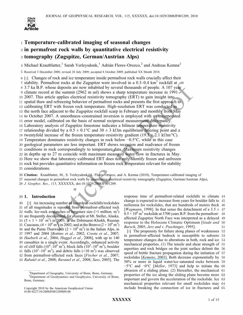
204 [9] Electrical resistivity as a function of temperature was205 measured in the laboratory using a 40 cm × 20 cm × 20 cm206 Wetterstein limestone cuboid sample taken from the study207 site. The Wetterstein limestone along the ERT transect is a208 fine‐grained dolomised limestone with a porosity of 4.42 ±209 0.41% and a permeability of 6.24 ± 1.12 mD and shows little210 vertical or lateral change in lithological properties. The

211sample was submerged in low conductive 0.032 (±0.002) S/m212water in a closed basin to approach its chemical equilibrium.213The pore space was fully saturated under atmospheric pres-214sure until (at 20°C) resistivity did not decline further. Free215saturation resembles the field situation more closely than216saturation under vacuum conditions [Sass, 1998]. The sample217was cooled and frozen in a freezing chamber in which the218temperature of the stone sample can be controlled with an219accuracy of 0.1–0.2°C in a range of 20°C to −4°C (Figure 4).220Ventilation was applied to avoid thermal layering. The221sample was loosely coated with a plastic film to minimize222drying. Two calibrated thermometers (Greisinger GMH2232000, with 0.03°C accuracy probes calibrated in an ice water224bath) were used to measure rock temperature during freezing.225Temperature probes were isolated with polystyrene and sili-226con from the surrounding air temperature. The rock temper-227ature inside the sample was recorded approximately at the228median depth of electric current flow (4.1 cm) for the229employed Wenner‐type four‐electrode configuration which230was estimated according to Barker [1989]. This array was231chosen for the resistance measurements as it resembles the232geometry of the fieldmeasurements. Stainless steel electrodes233of 5 mm diameter and 16 mm length were firmly placed in234holes drilled to a depth of 2–3 mm with a constant separation235of 8 cm. Four Wenner arrays were installed parallel on the236rock sample and were measured simultaneously to calculate

Figure 1. Map of the study site showing the ERT transect, geology, and features that were attributed topermafrost degradation after the Holocene climatic optimum (rockfall scarp) and at present. The Zug-spitze borehole is located directly under the black triangle at the summit. The new cog wheel train tunnelfollows a straight line from the doline (circle) to a point 300 m (directly) below the Zugspitze summit andthen proceeds in direction to the Gr. Riffelwandspitze.

KRAUTBLATTER ET AL.: QUANTITATIVE ERT OF PERMAFROST ROCKS XXXXXXXXXXXX

3 of 15

ArticleinProof

237 the mean deviation of resistivity. Galvanic contact was238 improved by adding conductive grease (Bosch) along the239 rock‐electrode contact. Resistance was measured in accor-240 dance with field measurements with an ABEM SAS 300B241 device at 0.2 mA and up to 160 V. To imitate natural con-242 ditions, we applied several freezing cycles. Resistivity was243 then calculated under the assumption of half‐space geometry.244 This assumption is justified given the dimensions of the rock

245samples. Deviations of current flow from real half‐space246conditions are expected to be in the range of 10% or less247according to depth of investigation models by Barker [1989]248and Roy [1972].

2493.2. ERT Data Acquisition

250[10] As outlined by Krautblatter and Hauck [2007],25110 mm diameter stainless steel electrodes were drilled 10 cm

Figure 2. (a) The 0.3–0.4 km3 wedge‐shaped rockfall scarp (dotted line) below the Zugspitze (2962 masl). The wedge starts in the top left part (Gr. Riffelwandspitze) as a steeply inclined sliding plane, coversthe whole width of the picture, and bottoms out at approximately 1900 m asl in the snow‐covered“Bayerisches Schneekar” Cirque. The transition from massive (tens of meter thick bedded) WettersteinLimestone to layered Muschelkalk sequences is visible at the bottom left part. (b) Position of the rockwall section monitored by ERT. Points 1 and 2 represent entrances to the gallery as shown in Figure 1.The rock wall outlined by the dotted line indicates the length of the transect monitored by ERT. Thesteep snow‐free rock face left of window (point 2) is the only part where undisturbed rock permafrostexists to date according to temperature and ERT measurements. A seasonally frozen rock body occursclose to the steep rock face at point 1.

Figure 3. MAAT of the Zugspitze meteorological station (2962 m asl) from 1991 to 2007 in comparisonto 30 year reference periods since 1901. Data indicate an abrupt rise in temperature in the last 17 years.

KRAUTBLATTER ET AL.: QUANTITATIVE ERT OF PERMAFROST ROCKS XXXXXXXXXXXX

4 of 15

ArticleinProof

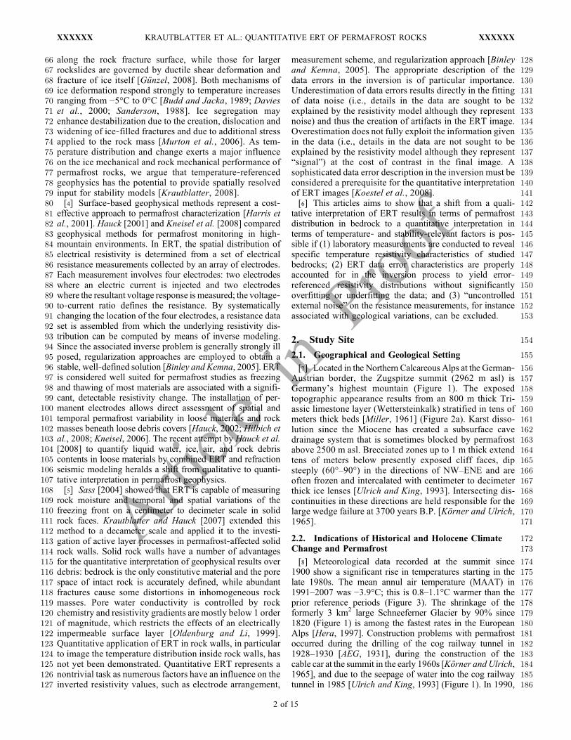
252 into the rock and firmly connected by electrode grease253 (Figure 5). Contact resistances range mostly between 100

254 and 102 W. The electrodes were placed in three arrays: the255 main array (61 electrodes) along a 276 m section of the main256 gallery, with an electrode spacing of 4.6 m (Figure 6). Two257 secondary arrays (41 electrodes each) with an electrode258 spacing of 1.533 m were located in the permafrost‐affected259 part. These arrays were installed parallel to the main gallery260 and perpendicular to the main gallery in the side gallery to261 improve the spatial resolution and coverage. In February262 2007, a total of 127 electrodes (16 electrodes of the different263 transects overlap) were installed to collect 750 resistance264 measurements with a Wenner array. Subsequently, mea-265 surements were performed with a high‐resolution array266 combining Wenner, Schlumberger, and Gradient config-267 urations, resulting in an average of 1550 measurements. Due268 to a lightning stroke, which damaged the instruments, the269 data set for June is reduced to 1050 measurements along the270 main gallery.

271 3.3. ERT Inversion

272 [11] ERT was processed using the 2‐D smoothness‐273 constrained inversion algorithm developed by Kemna274 [2000]. Here, inversion is accomplished by solving an275 optimization problem in which the model roughness is276 minimized subject to fitting the data to a predefined degree277 [LaBrecque et al., 1996]. Model roughness is quantified as278 the norm of the gradient of the log electrical conductivity279 distribution, lns(y, z), integrated over the considered two‐280 dimensional domain, which is evaluated on the basis of the281 given parameterization m of lns by a model roughness282 matrix Wm:

kWmmk2 �ZZ

kr2D ln�ð Þk2 dx dy ð1Þ

283 The regularization of the inverse problem by a smoothness284 constraint, i.e., the assumption of smooth model character-285 istics, represents a reasonable approach particularly for the

286present application, because in permafrost rocks thermal287diffusion along temperature gradients acts to smooth out288temperature‐induced gradients.289[12] The smoothness‐constrained inverse problem is solved290by minimizing the objective function

Y mð Þ ¼ Yd mð Þ þ � kWmmk2 ð2Þ

291by means of the Gauss‐Newton method [Kemna, 2000]. In292equation (2),Yd is the data misfit function and l the so‐called293regularization parameter which controls the influence of data294misfit versus model roughness in the objective function. The295data misfit is given as the misfit between the measured log296resistance data, d, and the corresponding predicted data, f(m),297for a given model m, weighted according to the individual298data uncertainties by a data weighting matrix Wd:

Yd ¼ kWd d� f mð Þð Þk2 ð3Þ

299[13] A diagonal weighting matrix is used, which corre-300sponds to the assumption of uncorrelated Gaussian data301errors. Their standard deviations are given by the inverse of302the entries of Wd, i.e., wii = "i

−1, where wii is the ith diagonal303element of Wd, "i is the standard deviation of the ith datum304di = lnRi, and Ri is the ith resistance measurement. Provided305that the correct standard deviations are used, an acceptable306data fit is achieved when the data misfit RMS (root‐mean‐307square) value

RMS ¼ Yd=Nð Þ1=2 ð4Þ

308is equal to one, where N is the number of given data points.309This approach, where the data are fitted to a well‐defined310degree based on an adequate data error description – in311contrast to the widely used approach of just minimizing the312data misfit – is essential for a quantitative interpretation of313ERT results.

Figure 4. Wetterstein limestone sample instrumented withelectrodes and high‐precision thermometers in the freezingchamber. Four parallel 24 cm long arrays are installed ona Wetterstein limestone sample that is coated with a plasticfilm to minimize drying.

Figure 5. Geophysical instrumentation in the Kammstollengallery 25 m from the north face at 2800 m asl. Permafrost isevident by perennial ice on the floor; electrodes and a tem-perature logger are shown on the right side.

KRAUTBLATTER ET AL.: QUANTITATIVE ERT OF PERMAFROST ROCKS XXXXXXXXXXXX

5 of 15

ArticleinProof

314 [14] The 2‐D ERT forward problem, defining the operator315 f in equation (3), is given by the 1‐D Fourier transform of316 the Poisson equation for a 3‐D point source in the image317 plane at (xs, ys) with current strength I:

@

@x�@�

@x

� �þ @

@y�@�

@y

� �� k2�� ¼ �I � x� xsð Þ� y� ysð Þ ð5Þ

318 In equation (5), k is the wave number corresponding to the319 assumed strike direction (z), � is the electric potential in the320 Fourier domain, and d is the Dirac delta function. For given321 boundary conditions, equation (5) is solved by means of the322 finite element (FE) method. The discretization accounts for323 the fact that each model cell of the parameterization is324 represented by a set of lumped finite elements. Once the325 transformed electric potential distribution is computed for326 each current injection position, inverse Fourier transform327 and appropriate superposition yields the transfer resistance

328Ri of any desired electrode configuration [Kemna, 2000].329The boundary conditions are generally expressed as

�@�

@nþ � � ¼ 0 ð6Þ

330where n denotes the outward normal and the parameter b331defines the type of boundary condition. We here impose a332no‐flow boundary condition (b = 0) at the rock face boundary333and so‐called mixed boundary conditions (b ≠ 0) at the grid334boundaries within the rock (Figure 6), where b is determined335based on the assumption that � behaves asymptotically as in336the homogeneous half‐space case [Dey and Morrison, 1979].337The finite element grid was designed to resemble the field338situation as closely as possible by accurate positioning of339electrodes along the rock galleries, mixed boundary condi-340tions toward the inner rock wall and no‐flow conditions at the341rock face (Figure 6).

Figure 6. ERT grid with 127 electrodes along the gallery. Different cell sizes refer to data sampling den-sity (electrode separation), and expected highest resolution is in the permafrost area close to the side gal-lery. Note that a no‐flow boundary condition is imposed at the rock face boundary (green line) and amixed boundary condition at the remaining grid boundaries inside the rock (red line). The color scaleof the ERT section is explained in Figure 11.

KRAUTBLATTER ET AL.: QUANTITATIVE ERT OF PERMAFROST ROCKS XXXXXXXXXXXX

6 of 15

ArticleinProof

342 3.4. ERT Data Error Characterization

343 [15] Errors in the ERT data can be both, systematic and344 random. Systematic errors involve a correlation of errors of345 different data in an ERT data set, or a correlation of data errors346 over time in time‐lapse ERT. They are associated with a347 malfunction of the measurement equipment, bad galvanic348 contact of electrodes, or misplaced or misconnected electro-349 des. Systematic errors should be rejected or corrected, before350 the inversion. Random errors, on the other hand, arise pri-351 marily from stochastic fluctuations in the contact between352 the electrodes with the air/ground, in the current injected, and353 due to changes in the current pathways [Slater et al., 2000].354 Random errors are uncorrelated and normally assumed to355 have a normal distribution (Gaussian noise).356 [16] An efficient procedure to characterize random error in357 geoelectrical measurements is based on the analysis of dif-358 ferences between measurements taken with normal and359 reciprocal configurations [Koestel et al., 2008; LaBrecque et

360al., 1996; Slater and Binley, 2006; Slater et al., 2000]. For a361given “normal” four‐electrode measurement configuration,362the reciprocal configuration applies swapped current and363voltage electrode pairs. Both measurements should be iden-364tical. In practice, they differ to some degree, and the deviation365can be considered as a measure of the present random error.366We here adopt the model of Slater et al. [2000] to describe the367data error, where the resistance error,DRi, is assumed to be a368linear function of the resistance Ri:

�Ri ¼ aþ bRi ð7Þ

369[17] In equation (7), parameter a represents an error370contribution in terms of absolute resistance (expressed in W),371dominating the error model for small resistances, and372parameter b, an error contribution in terms of relative373resistance (expressed in %), dominating the error model374for large resistances. Given the use of log‐transformed

Figure 7. Laboratory calibration of Wetterstein limestone from the Kammstollen study site. Four Wen-ner arrays (black, pink, orange, and green) with identical dimensions were installed on water‐saturatedlimestone and exposed to initial freezing, rethawing, and refreezing. (a) All measured data plotted as soliddots. All measured trajectories indicate a distinct knickpoint at the equilibrium freezing point at 30 kWmand −0.5°C. The higher unfrozen limb starting at 20°C (10 kWm) and falling to −0.5°C is the coolingpath; the lower unfrozen limb ending at 2°C (20 kWm) is the unfreezing path. (b) The results of initialfreezing. Solid dots indicate unfrozen values and supercooling between the equilibrium freezing point−0.5°C and the spontaneous freezing point −1.1°C. Spontaneous freezing occurs within 10 min with asudden warming of the sample of 0.7°C but little resistivity change. Frozen values are displayed as un-filled dots with the same color. (c) The results of refreezing experiments; note the absence of supercool-ing. For comparison, (d) initial freezing indicated as unfilled dots while solid dots with a highertemperature‐resistivity gradient represent refreezing values.

KRAUTBLATTER ET AL.: QUANTITATIVE ERT OF PERMAFROST ROCKS XXXXXXXXXXXX

7 of 15

ArticleinProof

375 data in the inversion, DRi is related to the data error "i376 according to

"i � �Ri

Ri¼ a

Riþ b ð8Þ

377 [18] The final inversion result depends strongly on the378 chosen parameters a and b. Overestimating the error present379 in the data will lead to a smooth, low‐resolution image due380 to underfitting of the data in the inversion. If the error is381 underestimated, the data will be overfitted and artifacts in382 the final image are likely to be generated. We follow the383 procedure of Koestel et al. [2008] to determine appropriate384 values for the parameters a and b. The range of resistances385 covered by the data set is subdivided into a number of386 “bins” (sub data sets). For each bin, the distribution of387 normal reciprocal differences (i.e., Rn − Rr, with Rn and Rr

388 denoting resistance measured with normal and reciprocal389 configuration) is statistically evaluated for its standard390 deviation. The linear model in equation (7) is then fitted to391 the obtained standard deviations for the different bins as a392 function of the mean resistance of the bins, yielding esti-393 mates for the parameters a and b. The diagonal entries of394 the data weighting matrix Wd in the inversion are then395 calculated from equation (8). We emphasize that this396 “calibration” of the error model for each individual data397 set is essential to avoid the creation of artifacts and398 guarantees consistency among data sets collected at dif-399 ferent times, allowing a quantitative interpretation of the400 obtained resistivity distributions.

401 3.5. Rock‐Wall Temperature Measurements

402 [19] Rock wall temperature probes were placed in the side403 gallery at a distance of 2.5, 5, 10, 15, and 20 m from the404 window in the north face (point 2 in Figure 6; see also405 Figure 5). The exits of the side gallery are closed at both406 sides by a wood construction. The probes were placed in407 40 cm deep boreholes that were sealed with silicon. We408 applied UTL II (GeoTest, 0.1°C accuracy) probes that

409were calibrated in ice water beforehand and data recording410was set to hourly intervals.

4114. Results

4124.1. Laboratory Temperature‐Resistivity Behavior413of Unfrozen, Supercooled, and Frozen Rocks

414[20] Figures 7a and 7d show that both, freezing and415refreezing of Wetterstein limestone occurs at −0.5 (±0.1) °C416and 30 (±3) kWm. When the sample is initially cooled fol-417lowing full saturation (initial freezing), the resistivity behavior418follows a linear trend from 22°C to 12°C (A in Figure 7) but419then remains constant from 12°C to the equilibrium freezing420point at −0.5°C (see B in Figure 7a and Discussion). During421initial freezing, supercooled conditions below the equilibrium422freezing point occur over a temperature range between423−0.5°C and −1.1°C, with a small resistivity decrease with424declining temperature (Figure 7b C). Spontaneous freezing425occurs with a sudden self‐induced increase of the temperature426of the rock sample by +0.6°C to −0.5°C due to latent heat427emission (Figure 7b D). After spontaneous freezing, a new428linear temperature‐resistivity behavior is evident with a much429steeper gradient (Figure 7b E). During melting and refreezing430of the limestone, unfrozen resistivities are significantly lower431than for initial freezing (Figure 7d B and F), no supercooling432below the equilibrium freezing point occurs and the resis-433tivity‐temperature gradient of frozen rock is steeper than for434initial freezing (Figure 7c G).435[21] Figure 8 shows that refrozen Wetterstein limestone436exhibits a steep resistivity‐temperature relationship with437small deviations (19.3 ± 2.1 kWm/°C). Temperature‐438dependent alterations of resistivity values in frozen rock439are much larger than internal deviations, while the oppo-440site is true for unfrozen resistivity‐temperature paths above441−0.5°C (Figure 7d B and F).

4424.2. Error Model Parameters

443[22] Figure 9 presents calculated standard deviations (DR)444of 3000 normal reciprocal measurements in bins as a func-445tion of their mean resistance. A linear model was fitted to

Figure 8. Mean resistivity values of refrozen Wetterstein limestone. Error bars indicate the mean devi-ation of refreezing resistivity values of the four arrays (Figure 7c “G”) from the mean value.

KRAUTBLATTER ET AL.: QUANTITATIVE ERT OF PERMAFROST ROCKS XXXXXXXXXXXX

8 of 15

ArticleinProof

446 obtain estimates for the error model parameters a and b. The447 bin analysis yields a = 48 W (absolute resistance error for448 small resistances) and b = 8.0% (relative resistance error for449 large resistances). Similar values are obtained, for a varying450 number of bins in the analysis. The error model parameters451 were used for the inversion of all data sets to ensure con-452 sistency among the ERT images at different times.

453 4.3. ERT Images

454 [23] The ERT record in 2007 starts after a 2.3°C warmer455 than average November to February winter period in com-456 parison to the mean of 1991–2007 (Figure 10). The observed457 period (February to October 2007) is 0.4°C warmer than458 average (1991–2007). From 1991 to 2007, February to459 October temperatures deviated on average by 1.5°C from the460 mean; thus, the temperatures of 2007 are well in the repre-461 sentative range for the last 17 years.

462 4.4. Absolute Resistivity Values

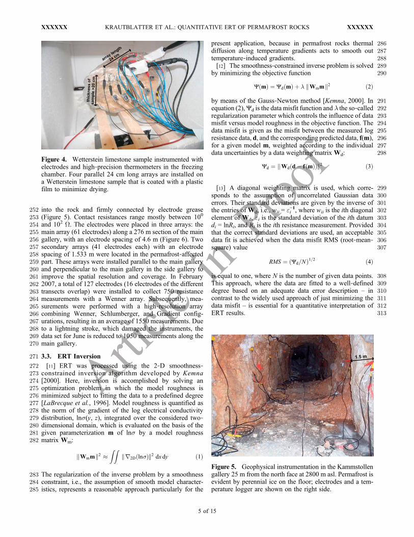
463 [24] In this specific case, changes in the degree of frac-464 turing or joint infillings appear to have no discernible465 influence on the resistivity distribution of the frozen rock

466mass (Figure 11). The gallery section, where perennial ice467and permafrost temperatures were found, appears as a cen-468tral high‐resistivity body from 50 m to 150 m with a pro-469nounced seasonal variation in resistivity. Resistivity values470greater than 104.5 Wm (≈laboratory value at −0.5°C), which471correspond to laboratory values of frozen rock, are con-472centrated close to the steep snow‐free rock face, while the473snow covered rock face yields resistivity values smaller than474104.5 Wm in all time frames. A seasonally frozen rock body475is found from 240 m to 276 m, also connected to a snow‐476free part of the rock face (Figure 2b, close to point 1). This477body shows a gradual reduction of resistivity away from the478rock face from February to June and disappears in July.479[25] The central perennial high‐resistivity body is char-480acterized by a core section of ≥104.7 Wm (≈laboratory value481at −2°C) and laterally aggrading or degrading of marginal482sections of ≥104.5 Wm (≈ laboratory value at −0.5°C).483February andMay, with rock temperature probe data between484−2°C and −4.5°C, yield the highest resistivity values of all485sections (≥104.95 Wm ≈ laboratory value at −3.5°C). Resis-486tivity values of 104.7 Wm slowly decrease, starting from the487rock face, and nearly disappear in August. Horizontal diffu-

Figure 9. Error model based on a bin analysis of the differences between normal and reciprocalmeasurements.

Figure 10. Mean monthly air temperature in 2006 and 2007 in comparison to 1991–2007 mean valuesand mean deviation.

KRAUTBLATTER ET AL.: QUANTITATIVE ERT OF PERMAFROST ROCKS XXXXXXXXXXXX

9 of 15

ArticleinProof

488 sion (y direction in Figure 10) of high resistivity values to489 27 m depth away from the rock face is observable until490 August, while lateral diffusion (x direction in Figure 10)491 peaks in May/June and is then substituted by a lateral con-492 traction of the marginal 104.5 Wm section in July/August.493 Resistivity increases in the permafrost lens are evident in494 September and diffuse to depth and laterally in October. In495 February, the high‐resistivity section broadens from 50 m to496 70 m toward the rock face. This trend reverses stepwise from497 May to August, with a pronounced narrowing toward the rock498 face of the 104.5Wm and 104.7Wm zone developed in August,499 and reappears in September coincidently with the drop of500 the mean monthly air temperatures below 0°C (Figure 10).501 The fractured section to the left of the side gallery (50–90 m)502 indicates an abrupt decrease in resistivity in May.

503 4.5. Absolute Resistivity Changes

504 [26] The most pronounced change in resistivity occurs505 between February and May (Figure 12). Resistivities values

506decrease rapidly in the 50–90 m section (note that the507tomography covers three months), while the section from508100 to 150 m still shows a moderate increase of resistivity.509Between May and July the decrease of resistivity values510occurs mainly in the central high‐resistivity section (80–511140 m) and is more intense close to the rock surface. From512July to August, a rapid decrease of resistivity values occurs at513all depths in the central permafrost body. The cool September514(Figure 10) reverses this trend and initiates resistivity515increase close to the central high‐resistivity body (60–95 m).516Only small resistivity changes are observed in October.

5174.6. Rock‐Wall Temperature Data

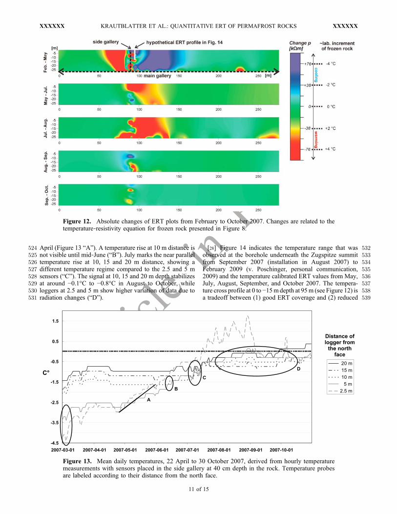
518[27] The temperature sensors, inserted at a depth of 40 cm519in the rock in the side gallery, give some indication of the520general temperature regime but they do not measure the521undisturbed rock temperature. Temperature probes located522at distances of 2.5 and 5 m from the Zugspitze North Face523show an abrupt linear temperature rise starting at the end of

Figure 11. ERT inversion results based on 127 electrodes and on average 1550 resistance measurementsper ERT frame. Because of a lightning damage of instruments in the side gallery, the image for June has alower resolution between 55 m and 135 m. The bar below shows sections where fracture zones with jointapertures >2 mm were mapped along the gallery irrespective of their orientation.

KRAUTBLATTER ET AL.: QUANTITATIVE ERT OF PERMAFROST ROCKS XXXXXXXXXXXX

10 of 15

ArticleinProof

524 April (Figure 13 “A”). A temperature rise at 10 m distance is525 not visible until mid‐June (“B”). July marks the near parallel526 temperature rise at 10, 15 and 20 m distance, showing a527 different temperature regime compared to the 2.5 and 5 m528 sensors (“C”). The signal at 10, 15 and 20 m depth stabilizes529 at around −0.1°C to −0.8°C in August to October, while530 loggers at 2.5 and 5 m show higher variation of data due to531 radiation changes (“D”).

532[28] Figure 14 indicates the temperature range that was533observed at the borehole underneath the Zugspitze summit534from September 2007 (installation in August 2007) to535February 2009 (v. Poschinger, personal communication,5362009) and the temperature calibrated ERT values from May,537July, August, September, and October 2007. The tempera-538ture cross profile at 0 to −15m depth at 95m (see Figure 12) is539a tradeoff between (1) good ERT coverage and (2) reduced

Figure 12. Absolute changes of ERT plots from February to October 2007. Changes are related to thetemperature‐resistivity equation for frozen rock presented in Figure 8.

Figure 13. Mean daily temperatures, 22 April to 30 October 2007, derived from hourly temperaturemeasurements with sensors placed in the side gallery at 40 cm depth in the rock. Temperature probesare labeled according to their distance from the north face.

KRAUTBLATTER ET AL.: QUANTITATIVE ERT OF PERMAFROST ROCKS XXXXXXXXXXXX

11 of 15

ArticleinProof

540 thermal influence from air circulation in the main and side541 gallery. ERT values were transformed into temperature using542 the equation given in Figure 8. Data sets from February and543 June are not displayed as the side gallery was not shielded by544 wooden doors before February and is, thus, heavily disturbed545 (see side gallery in Figure 11, top) and nomeasurements were546 taken in the side gallery in June due to the lightning damage.547 Figure 14 shows that there is a good correspondence of both548 methods for the upper limit of permafrost temperatures549 around −3°C, while data on minimum temperatures signifi-550 cantly differ.

551 5. Discussion

552 [29] McGinnis et al. [1973] suggested an exponential for-553 mula for the temperature‐resistivity behavior of bedrock.554 Their data derived from 10°C to 20°C increment laboratory555 measurements using Berea sandstones and limestones and556 did not precisely target on temperatures around the freezing557 point. Our laboratory data at 0.1–0.2°C increments indicate558 that freezing of low‐porosity rocks is better approached by a559 bilinear relationship divided at a freezing point significantly560 below 0°C.561 [30] 1. The resistivity increase from 22 to 12°C follows562 the linear relation postulated by Keller and Frischknecht563 [1966].564 [31] 2. The resistivity remains constant from 12°C to 0°C,565 possibly due to increasing conductivity of pore water566 resulting from enhanced carbonate solution at lower tem-567 peratures. This hypothesis is supported by the fact that we568 found this behavior in our studies only in carbonate samples569 and that the resistivity of thawing limestone is much lower

570than the resistivity of initially cooling limestone (Figure 7d,571“B” and “F”).572[32] 3. The depression of the equilibrium freezing point573below 0°C in rocks was not resolved in prior studies that574targeted rock resistivity [McGinnis et al., 1973; Mellor,5751973]. Petrophysical studies show that the lowering of the576equilibrium freezing point in confined porous media is577dependent on pore space and pore material [Sliwinska‐578Bartkowiak et al., 2008].579[33] 4. Supercooled conditions (−0.5°C to −1.1°C) may be580explained by excessive pore pressure build up in pores fully581saturated with water or by metastable supercooling effects582[Lock, 2005]. Supercooling occurs only during initial freez-583ing and not when refreezing. This points toward excessive584pore pressure build up and pore water extrusion coinciding585with instantaneous freezing.586[34] 5. The jump of resistivity at the freezing point and the587bilinear temperature‐resistivity relation for saturated natural588rocks is evident in data provided by Mellor [1973] but has589been poorly adapted since that. Both initial freezing and590refreezing of water‐saturated Wetterstein limestone yielded591an equilibrium freezing point at −0.5 ± 0.1°C with resistivity592values close to 30 ± 3 kWm. The resistivity of unfrozen593Wetterstein limestone increases by less than 104 Wm/°C,594while the resistivity of the refrozen specimen increases on595average by 19.1 (±0.6) × 104 Wm/°C. As rocks at the study596site have been exposed to repeated freezing, we assume597that the refreezing curve is relevant for the calibration of598ERT values. The refreezing curve is a good target for599temperature‐referencing of ERT results as the temperature600gradient of 19.1 × 104 Wm/°C is 30 times larger than601the mean deviation due to internal lithological variability602(±0.6 × 104 Wm/°C).

Figure 14. Comparison of the temperature range obtained by borehole data (temperature probe spacing,see diagram) at the Zugspitze summit north face (2920 m asl) and by temperature‐calibrated ERT at theKammstollen North Face (2800 m asl, position see Figure 12). This hypothetical ERT profile is theclosest analog to the borehole situation with the same aspect in 300 m distance and with an altitudinaldifference of 100 m.

KRAUTBLATTER ET AL.: QUANTITATIVE ERT OF PERMAFROST ROCKS XXXXXXXXXXXX

12 of 15

ArticleinProof

603 [35] Few publications target the problem of transferring604 laboratory‐scale electrical experiments to a decameter field605 scale [Day‐Lewis et al., 2005; Singha and Gorelick, 2006].606 Zisser et al. [2007] showed that pore volume, degree of607 interconnection of the pores through pore throats, and the608 distribution and orientation of open cracks and fractures609 determine electrical properties of limestone. Resistivity610 values of jointed rock masses in the field may vary from the611 resistivity values of intact laboratory samples. Jouniaux et612 al. [2006] showed that stress‐induced crack formation in613 intact saturated limestone increases electrical conductivity614 by up to 4%. However, a survey of joint width, spacing615 orientation and joint infillings along the monitored main616 gallery showed little correspondence to the ERT behavior of617 frozen rock (see Figure 9). This is likely due to homoge-618 neous lithological conditions in the Wetterstein limestone619 [Miller, 1961] and the application of this method in more620 heterogeneous rock sequences will require more geological621 input into the resistivity model.622 [36] A bin analysis of misfits against average of normal623 and reciprocal measurements [Binley et al., 1995] yielded an624 absolute error of 48 W and a relative error of 8.0%. These are625 reasonable values considering the high resistances (up to626 5 kW) measured. As the interpretation focuses on values627 greater than 104.5 Wm, the relative error of 8.0% is the rel-628 evant error parameter. Laboratory experiments by Koestel et629 al. [2008] derived relative errors of up to 1.1%. The error630 parameters in this study were obtained in the same way but631 we used a different number of bins for the analysis, which632 reflects the stability of the parameters in a range of measured633 resistances. Employed error model settings appear to be634 capable of avoiding underestimations or overestimations635 over the entire range of values. Smoothness‐constrained636 inversion of the data with the error model setting shows637 consistent results for all different data sets and resolutions.638 [37] A shift from qualitative to quantitative interpretation639 of geophysical results, as heralded by Hauck et al. [2008],640 appears to be possible for frozen permafrost‐affected bed-641 rock. All incorporated values lie within a realistic range in642 comparison to borehole temperature data (Figure 14). The643 images gained appear to be free of artifacts and their high644 resolution permits the detection of seasonal resistivity645 changes in frozen rock. Consistent with the rock and air646 temperature data, the absolute ERT plots show that the main647 thawing occurred from May to August with a significant648 retreat of high‐resistivity sections above 104.7Wm (≈lab value649 at −2°C) to distances of 20 m inward from the rock face. The650 onset of thawing processes in May, subsequent to the warm651 April, is pronounced by resistivity decreases corresponding to652 5°C (95 kWm) and more (Figure 12). The speed of tempera-653 ture change cannot be explained by heat conduction alone654 [Noetzli et al., 2007] and is concentrated close to a fracture655 zone with open (>2 mm) joints (60–80 m). Coincidently,656 significant joint water seepage into the gallery below the657 permafrost body was measured on 20 May. Water of 2.5–658 3.8°C seeped with a maximum discharge of 0.28 l/min659 at 1800 LT from a 34 cm long joint with an aperture of 2–660 3.5 cm. We hypothesize that the deep‐reaching decline in661 resistivity is due to meltwater percolation in joints trans-662 porting large amounts of latent and sensible heat (i.e.,663 advective heat transfer). Daily variations of joint water664 seepage below a rock mass, tens of meters thick, indicate

665rapid percolation through a highly permeable joint system,666as previously observed by Wegmann [1998]. Three‐667dimensional effects due to rock wall topography [Gruber668and Haeberli, 2007] could also act to accelerate response669times. A deep‐reaching thawing response is apparent in the670plot of August–July resistivity change also in the part of671the rock face that was covered by snow until mid‐July672(Figure 10). In the cold September and October, resistivity673increases around the permafrost body and resistivity values674greater than 104.7 Wm (≈lab value at −2°C) reappear675between the permafrost body and the north face. The exis-676tence of the galleries may locally influence the thermal677regime, but their impact is too small to affect much of the67860*20 m wide and decameter thick permafrost lens. Local679authorities (Bayerische Zugspitzbahn AG) report that the680main gallery was perennially floored with ice along the681whole observed transect in the 1970s and that the length of682frozen section of the main gallery decreased enormously in683summer 2003.684[38] Apparent resistivities up to 105.2 Wm alongside gal-685lery sections with cm thick ice‐filled joints and calculated686resistivities up to 105.3 Wm in the fracture zone at 60–80 m687from 0 to −20 m depth show that anisotropy along ice‐filled688fractures in the rock mass can disturb the electrical mea-689surements. Tensorial nonconductivity of ice‐filled joints of690unknown orientation may cause series disconnection or691parallel disconnection and influences resistivity in a yet not692exactly determined way [Matias, 2008]. Superficial apparent693resistivity values measured in the side gallery are affected by694ice in fractures, and temperature data obtained from the side695gallery are distorted by air circulation. Thus, a comparison696of temperature probe point data with ERT data (that mea-697sures average resistivity of several cubic meters of rock698volume) is not possible. However, borehole data from the699Zugspitze summit and temperature‐calibrated ERT provide700similar “core” permafrost temperatures (−3°C to −4°C) at70110–15 m from the north face (Figure 14). A comprehensive702understanding of the thermal regime that is indicated by the703ERT time sections requires an enhanced measurement704scheme of surface temperatures and joint water influence as705well as 3‐D modeling of thermal data. ERT could help to706calibrate and validate 3‐D thermal modeling inputs and707outputs and while 3‐D thermal modeling and geophysical708forward modeling could help to test the limitations of the709described ERT method.710[39] While GPR and seismic surveys are well implemented711in the stability considerations of rock mass properties712[Heincke et al., 2006a, 2006b], ERT has only been applied713in a few cases and solely in the in the context of fracture714characterization [Choi et al., 2006;Deparis et al., 2008]. As715soon as ERT data can be correlated reliably to temperature of716frozen rock, the link between temperature, rock mechanics717and icemechanics opens up a new application for geophysical718stability analysis.

7196. Conclusion

720[40] High‐resolution ERT with 127 electrodes and on721average 1550 datum points was conducted along a 276 m722long gallery in the permafrost‐affected north face of the723Zugspitze in 2800 m asl in February, May, June, July,724August, September, and October 2007. Data inversion was

KRAUTBLATTER ET AL.: QUANTITATIVE ERT OF PERMAFROST ROCKS XXXXXXXXXXXX

13 of 15

ArticleinProof

725 performed using an 8400 finite element grid with adjusted726 boundary conditions. In order to process quantitatively727 reliable ERT values, we fitted a smoothness‐constrained728 Occam’s inversion to an empirically measured normal729 reciprocal error model. Water‐saturated Wetterstein lime-730 stone was measured in the laboratory to freeze at −0.5 ±731 0.1°C with resistivity values close to 30 (±3) kWm. The732 temperature‐resistivity relationship of repeatedly frozen733 limestone below −0.5°C can be described by p [in kWm] =734 19.1 – 19.3 ± 2.1 × t [C°] with an R2 of 0.99. This equation735 was used to reference the ER tomographies along the per-736 mafrost gallery. Absolute resistivity values and monthly737 resistivity changes are generally consistent with seasonal738 air temperature changes and rock temperatures observed in739 the adjacent borehole. Differences in snow coverage dom-740 inate the general distribution of permafrost. Pronounced741 thaw occurs from May to August. Rapid melting occurs742 along fracture zones at the same time as joint water seepage743 into the gallery in May. Refreezing from the rock face starts744 in September and is apparent in both, increasing resistivity745 values and the expansion of the high‐resistivity body.746 Temperature‐resistivity calibration in the laboratory and747 error‐controlled inversion of high‐resolution ERT field748 data present the first step toward quantitative temperature‐749 referenced geophysics in permafrost rocks.

750 [41] Acknowledgments. Special thanks to A v. Poschinger from the751 Bayerisches Landesamt fuer Umwelt (LFU) and to M. Hurm (Bayerische752 Zugspitzbahn AG) for their friendly support. We gratefully acknowledge753 financial support from the DFG (German Research Council) as part of754 the projects “Sensitivity of rock permafrost to climate change and implica-755 tions for rock wall stability” and the graduate school 437 “Relief.” We are756 indebted to R. Dikau for steady support, discussions, and valuable advice.757 This paper profited much from the comments of O. Sass, two anonymous758 reviewers, the Editor M. Church, and Associate Editor E. Moore.

759 References760 AEG (1931), Die Bayerische Zugspitzbahn, 88 pp., Berlin.761 Barker, R. D. (1989), Depth of investigation of collinear symmetrical four‐762 electrode arrays, Geophysics, 54(8), 1031–1037, doi:10.1190/1.1442728.763 Binley, A., and A. Kemna (2005), Electrical methods, in Hydrogeophysics,764 edited by Y. Rubin and S. S. Hubbard, pp. 129–156, Springer, Dordrecht,765 Netherlands.766 Binley, A., A. Ramiraz, and W. Daily (1995), Regularised image recon-767 struction of noisy electrical resistance tomography data, paper presented768 at 4th Workshop of the European Concerted Action on Process Tomog-769 raphy, Univ. of Bergen, Bergen, Norway.770 Bottino, G., M. Chiarle, A. Joly, and G. Mortara (2002), Modelling rock771 avalanches and their relation to permafrost degradation in glacial772 environments, Permafrost Periglacial Processes, 13(4), 283–288,773 doi:10.1002/ppp.432.774 Budd, W. F., and T. H. Jacka (1989), A review of ice rheology for ice‐sheet775 modeling, Cold Reg. Sci. Technol., 16, 107–144, doi:10.1016/0165-232X776 (89)90014-1.777 Choi, J. S., H. H. Ryu, I. M. Lee, and G. C. Cho (2006), Rock mass clas-778 sification using electrical resistivity: An analytical study, in Advanced779 Nondestructive Evaluation, edited by S. S. Lee et al., pp. 1411–1414,780 Trans. Tech. Publ. LTD, Zurich, Switzerland.781 Crosta, G. B., O. Hungr, R. Sosio, and P. Frattini (2007), Dynamic analysis782 of the Punta Thurwieser rock avalanche, Geophys. Res. Abstr., 9, 09602.783 Davies, M. C. R., O. Hamza, B. W. Lumsden, and C. Harris (2000), Lab-784 oratory measurements of the shear strength of ice‐filled rock joints, Ann.785 Glaciol., 31, 463–467, doi:10.3189/172756400781819897.786 Day‐Lewis, F. D., K. Singha, and A. M. Binley (2005), Applying petrophy-787 sical models to radar travel time and electrical resistivity tomograms:788 Resolution‐dependent limitations, J. Geophys. Res., 110, B08206,789 doi:10.1029/2004JB003569.790 Deparis, J., et al. (2008), Combined use of geophysical methods and remote791 techniques for characterizing the fracture network of a potentially unsta-

792ble cliff site (the ‘Roche du Midi’, Vercors massif, France), J. Geophys.793Eng., 5(2), 147–157, doi:10.1088/1742-2132/5/2/002.794Dey, A., and H. F. Morrison (1979), Resistivity modelling for arbitrarily795shaped two‐dimensional structures, Geophys. Prospect., 27, 106–136,796doi:10.1111/j.1365-2478.1979.tb00961.x.797Fischer, L., C. Huggel, and F. Lemy (2007), Investigation and modeling of798periglacial rock fall events in the European Alps, Geophys. Res. Abstr., 9,79908160.800Gruber, S., and W. Haeberli (2007), Permafrost in steep bedrock slopes and801its temperature‐related destabilization following climate change, J. Geophys.802Res., 112, F02S13, doi:10.1029/2006JF000547.803Gude, M., and D. Barsch (2005), Assessment of the geomorphic hazards in804connection with permafrost occurrence in the Zugspitze area (Bavarian805Alps, Germany), Geomorphology, 66(1–4), 85–93, doi:10.1016/j.806geomorph.2004.03.013.807Günzel, F. (2008), Shear strength of ice‐filled rock joints, paper presented808at 9th International Conference on Permafrost, Inst. of Northern Eng.,809Univ. Alaska Fairbanks, Fairbanks, Alaska.810Haeberli, W., et al. (2004), The Kolka‐Karmadon rock/ice slide of 20811September 2002: An extraordinary event of historical dimensions in812North Ossetia, Russian Caucasus, J. Glaciol., 50, 533–546, doi:10.3189/813172756504781829710.814Harris, C., M. C. R. Davies, and B. Etzelmüller (2001), The assessment of815potential geotechnical hazards associated with mountain permafrost in a816warming global climate, Permafrost Periglacial Processes, 12(1), 145–817156, doi:10.1002/ppp.376.818Hauck, C. (2001), Geophysical methods for detecting permafrost in high819mountains, Ph.D. thesis, 204 pp., ETH Zurich, Zurich, Switzerland.820Hauck, C. (2002), Frozen ground monitoring using DC resistivity tomogra-821phy, Geophys. Res. Lett., 29(21), 2016, doi:10.1029/2002GL014995.822Hauck, C., M. Bach, and C. Hilbich (2008), A four‐phase model to quan-823tify subsurface ice content in permafrost regions based on geophysical824data sets, paper presented at 9th International Conference on Permafrost,825Inst. of Northern Eng., Univ. Alaska Fairbanks, Fairbanks, Alaska.826Heincke, B., A. G. Green, J. van der Kruk, and H. Willenberg (2006a),827Semblance‐based topographic migration (SBTM): A method for identifying828fracture zones in 3‐D georadar data, Near Surface Geophys., 4(2), 79–88.829Heincke, B., et al. (2006b), Characterizing an unstable mountain slope using830shallow 2‐D and 3‐D seismic tomography, Geophysics, 71(6), B241,831doi:10.1190/1.2338823.832Hera, U. (1997), Gletscherschwankungen in den Nördlichen Kalkalpen seit833dem 19. Jh., Muenchner Geogr. Abh., Reihe B, 25, 1–205.834Hilbich, C., et al. (2008), Monitoring mountain permafrost evolution using835electrical resistivity tomography: A 7‐year study of seasonal, annual, and836long‐term variations at Schilthorn, Swiss Alps, J. Geophys. Res., 113,837F01590, doi:10.1029/2007JF000799.838Huggel, C., S. Gruber, J. Caplan‐Auerbach, R. L. Wessels, and B. F. Molnia839(2008), The 2005 Mt. Steller, Alaska, rock‐ice avalanche: A large slope840failure in cold permafrost, paper presented at 9th International Conference841on Permafrost, Inst. of Northern Eng., Univ. Alaska Fairbanks, Fairbanks,842Alaska.843Jerz, H., and A. v. Poschinger (1995), Neuere Ergebnisse zum Bergsturz844Eibsee‐Grainau, Geol. Bavarica, 99, 383–398.845Jouniaux, L., M. Zamora, and T. Reuschle (2006), Electrical conductivity846evolution of non‐saturated carbonate rocks during deformation up to847failure, Geophys. J. Int., 167(2), 1017–1026, doi:10.1111/j.1365-848246X.2006.03136.x.849Keller, G. V., and F. C. Frischknecht (1966), Electrical Methods in Geo-850physical Prospecting, 519 pp., Pergamon Press, Oxford.851Kemeny, J. (2003), The time‐dependent reduction of sliding cohesion due852to rock bridges along discontinuities: A fracture mechanics approach,853Rock Mech. Rock Eng., 36(1), 27–38, doi:10.1007/s00603-002-0032-2.854Kemna, A. (2000), Tomographic inversion of complex resistivity—Theory855and application, Ph.D. thesis, Univ. of Bochum, Bochum, Germany.856Kneisel, C. (2006), Assessment of subsurface lithology in mountain857environments using 2D resistivity imaging, Geomorphology, 80(1–2),85832–44, doi:10.1016/j.geomorph.2005.09.012.859Kneisel, C., C. Hauck, R. Fortier, and B. Moorman (2008), Advances in860geophysical methods for permafrost investigations, Permafrost and Peri-861glacial Processes, 19(2), 157–178, doi:10.1002/ppp.616.862Koestel, J., A. Kemna, M. Javaux, A. Binley, and H. Vereecken (2008),863Quantitative imaging of solute transport in an unsaturated and undis-864turbed soil monolith with 3D ERT and TDR, Water Resour. Res., 44,865W12411, doi:10.1029/2007WR006755.866Körner, H., and R. Ulrich (1965), Geologische und felsmechanische867Untersuchungen für die Gipfelstation der Seilbahn Eibsee ‐ Zugspitze,868Geol. Bavarica, 55, 404–421.869Krautblatter, M. (2008), Rock permafrost geophysics and its explanatory870power for permafrost‐induced rockfalls and rock creep: A perspective,

KRAUTBLATTER ET AL.: QUANTITATIVE ERT OF PERMAFROST ROCKS XXXXXXXXXXXX

14 of 15

ArticleinProof

871 paper presented at 9th International Conference on Permafrost, Inst. of872 Northern Eng., Univ. Alaska Fairbanks, Fairbanks, Alaska.873 Krautblatter, M., and C. Hauck (2007), Electrical resistivity tomography874 monitoring of permafrost in solid rock walls, J. Geophys. Res., 112,875 F02S20, doi:10.1029/2006JF000546.876 LaBrecque, D. J., M. Miletto, W. Daily, A. Ramirez, and E. Owen (1996),877 The effects of noise on Occam’s inversion of resistivity tomography data,878 Geophysics, 61(2), 538–548, doi:10.1190/1.1443980.879 Lock, G. S. H. (2005), The Growth and Decay of Ice, Cambridge Univ.880 Press, Cambridge, U. K.881 Matias, M. J. S. (2008), Electrical strike imaging and anisotropy diagnosis882 from surface resistivity measurements, Near Surf. Geophys., 6(1), 49–58.883 McGinnis, L. D., K. Nakao, and C. C. Clark (1973), Geophysical identifi-884 cation of frozen and unfrozen ground, Antarctica, paper presented at 2nd885 International Conference on Permafrost, Int. Permafrost Assoc., Yakutsk,886 Russia.887 Mellor,M. (1973),Mechanical properties of rocks at low temperatures, paper888 presented at 2nd International Conference on Permafrost, Int. Permafrost889 Assoc., Yakutsk, Russia.890 Miller, H. (1961), Der Bau des westlichen Wettersteingebirges, Z. Dtsch.891 Geol. Ges., 113, 409–425.892 Murton, J. B., R. Peterson, and J.‐C. Ozouf (2006), Bedrock fracture by ice893 segregation in cold regions, Science, 314, 1127–1129, doi:10.1126/894 science.1132127.895 Noetzli, J. (2008), Modeling transient three‐dimensional temperature fields in896 mountain permafrost, Ph.D. thesis, Univ. of Zurich, Zurich, Switzerland.897 Noetzli, J., S. Gruber, T. Kohl, N. Salzmann, and W. Haeberli (2007),898 Three‐dimensional distribution and evolution of permafrost temperatures899 in idealized high‐mountain topography, J. Geophys. Res., 112, F02S13,900 doi:10.1029/2006JF000545.901 Oldenburg, D. W., and Y. G. Li (1999), Estimating depth of investigation902 in DC resistivity and IP surveys, Geophysics, 64(2), 403–416,903 doi:10.1190/1.1444545.904 Rabatel, A., P. Deline, S. Jaillet, and L. Ravanel (2008), Rock falls in high‐905 alpine rock walls quantified by terrestrial lidar measurements: A case906 study in the Mont Blanc area, Geophys. Res. Lett., 35, L10502,907 doi:10.1029/2008GL033424.908 Ravanel, L., P. Deline, S. Jaillet, and A. Rabatel (2008), Quantifying rock909 falls/avalanches in steep high‐alpine rock walls: Three years of laserscan-910 ning in the MontBlanc massif, Geophys. Res. Abstr., 10, 10361.911 Roy, A. (1972), Depth of investigation in Wenner, three‐electrode and912 dipole‐dipole DC resistivity methods, Geophys. Prospect., 20, 329–913 340, doi:10.1111/j.1365-2478.1972.tb00637.x.

914Sanderson, T. (1988), Ice Mechanics and Risks to Offshore Structures,915272 pp., Springer, Amsterdam.916Sass, O. (1998), Die Steuerung von Steinschlagmenge durch Mikroklima,917Gesteinsfeuchte und Gesteinseigenschaften im westlichen Karwendelge-918birge, Münchner Geogr., Abh. Reihe B, 29, 1–175.919Sass, O. (2004), Rock moisture fluctuations during freeze‐thaw cycles: Pre-920liminary results from electrical resistivity measurements, Polar Geogr.,92128(1), 13–31, doi:10.1080/789610157.922Sass, O. (2005), Spatial patterns of rockfall intensity in the northern Alps,923Z. Geomorphol., 138, 51–65.924Singha, K., and S. M. Gorelick (2006), Effects of spatially variable resolu-925tion on field‐scale estimates of tracer concentration from electrical inver-926sions using Archie’s law, Geophysics, 71(3), G83, doi:10.1190/9271.2194900.928Slater, L., and A. Binley (2006), Synthetic and field‐based electrical imag-929ing of zerovalent iron barrier: Implications for monitoring long‐term bar-930rier performance, Geophysics, 71, B129, doi:10.1190/1.2235931.931Slater, L., A. Binley, W. Daily, and R. Johnson (2000), Cross‐hole electri-932cal imaging of a controlled saline tracer injection, J. Appl. Geophys., 44,93385–102, doi:10.1016/S0926-9851(00)00002-1.934Sliwinska‐Bartkowiak, M., M. Jazdzewska, L. L. Huang, and K. E. Gubbins935(2008), Melting behavior of water in cylindrical pores: Carbon nanotubes936and silica glasses, Phys. Chem. Chem. Phys., 10(32), 4909–4919,937doi:10.1039/b808246d.938Ulrich, R., and L. King (1993), Influence of mountain permafrost on con-939struction in the Zugspitze mountains, Bavarian Alps, Germany, paper940presented at 6th International Conference on Permafrost, Chinese Soc.941Glaciol. and Geocryol., Beijing.942Wegmann,M. (1998), Frostdynamik in hochalpinen Felswänden amBeispiel943der Region Jungfraujoch ‐ Aletsch, Ph.D. thesis, 144 pp., ETH Zurich,944Zurich, Switzerland.945Zisser, N., G. Nover, H. Durrast, and S. Siegesmund (2007), Relationship946between electrical and hydraulic properties of sedimentary rocks,947Z. Dtsch. Ges. Geowiss., 158(4), 883–894, doi:10.1127/1860-1804/9482007/0158-0883.

949A. Flores‐Orozco and A. Kemna, Department of Geodynamics and950Geophysics, University of Bonn, D‐53012 Bonn, Germany.951M. Krautblatter and S. Verleysdonk, Department of Geography,952University of Bonn, D‐53012 Bonn, Germany.

KRAUTBLATTER ET AL.: QUANTITATIVE ERT OF PERMAFROST ROCKS XXXXXXXXXXXX

15 of 15