Technology Shocks, Employment, and Labor Market Frictions

Technology Shocks, Employment, and Labor Market Frictions�

Federico S. Mandelmany

Federal Reserve Bank of Atlanta

Francesco Zanettiz

Bank of England

December 2007

Abstract

Recent empirical evidence suggests that a positive technology shock leads to a decline

in labor inputs. However, the standard real business model fails to account for this

empirical regularity. Can the presence of labor market frictions address this problem,

without otherwise altering the functioning of the model? We develop and estimate a real

business cycle model using Bayesian techniques that allows, but does not require, labor

market frictions to generate a negative response of employment to a technology shock.

The results of the estimation support the hypothesis that labor market frictions are the

factor responsible for the negative response of employment.

JEL Classi�cation: E32.

Keywords: Technology shocks, employment, labor market frictions.

�We wish to thank Bob Hills and Pedro Silos for helpful comments and suggestions. M. Laurel Graefeprovided superb research assistantship. This paper represents the views and analysis of the authors andshould not be thought to represent those of the Bank of England, the Monetary Policy Committee members,the Federal Reserve Bank of Atlanta, or the Federal Reserve System.

yFederico S. Mandelman, Federal Reserve Bank of Atlanta, Research Department, 1000 Peachtree Street,N.E. Atlanta, GA 30309-4470, USA. Tel: +1-404-498-8785. Email: [email protected].

zFrancesco Zanetti, Bank of England, Threadneedle Street, London, EC2R 8AH, UK. Tel: +44-(0)-207-601-5602. Email: [email protected].

1

1 Introduction

A key question in macroeconomics is what driving forces generate aggregate �uctuations. Ac-

cording to the real business cycle (RBC) paradigm initiated by Kydland and Prescott (1982),

cycles are generated by persistent shocks to technology; other shocks are either absent or have

a minimal role in explaining aggregate �uctuations. A key feature of this theoretical frame-

work is the positive response of employment to technology shocks, as documented by King

and Rebelo (2000). Recent empirical evidence, however, con�icts with this prediction. Galí

(1999), using long-run restrictions on a structural VAR, where a technology shock is identi�ed

as the only shock that a¤ects labor productivity in the long-run, shows that technology shocks

have a contractionary e¤ect on employment. In addition, Francis and Ramey (2005), Liu and

Phaneuf (2006), Wang and Wen (2007), and Whelan (2004) �nd that this result is robust

to di¤erent speci�cations of the VAR and the measure of productivity used. Moreover, Shea

(1998) and Basu, Fernald, and Kimball (2004) �nd similar evidence by measuring technology

with �Solow residuals� derived from microdata. More recently, Canova, López-Salido and

Michelacci (2007) and López-Salido and Michelacci (2007) show that a structural VAR model

that incorporates job �ows also generates a negative response of employment to technology

shocks.1 On the basis of this stylized fact, the validity of the RBC paradigm could be called

into question.

A possible way to reconcile the RBC paradigm with this stylized empirical fact is to amend

the standard model such that it generates a negative reaction of employment to a technol-

ogy shock, but still preserves its original functioning. In this spirit, Hairault, Longot and

Portier (1997) embed implementation lags in the adoption of new technology into a standard

RBC model to make future productivity higher than the current level, thereby decreasing

1Nonetheless, the debate on this �nding is still open. See, among others, Christiano Eichenbaum andVigfusson (2004), McGrattan (2004), Chari, Kehoe, McGrattan (2005), and Alexopoulos (2006).

2

current labor supply for a given increase in labor demand and, consequently, generating a

negative response of employment to a technology shock. Francis and Ramey (2005) introduce

habit formation in consumption together with adjustment costs on investment, and Leontief

technology with variable utilization to match the negative e¤ect of a technology shock on

employment. Lindé (2004) observes that if the process for a permanent technology shock is

persistent in growth rates, labor inputs fall on impact. More recently, Collard and Dellas

(2007), using an international RBC model, show that if the degree of substitution between

domestic and foreign goods is low, the reaction of employment to a technology shock is neg-

ative. Finally, Wang and Wen (2007) show that a RBC model with �rm entry and exit in

which �rms need time-to-build before earning pro�ts also delivers a negative response of em-

ployment to a technology shock. All these works show that by appropriately modifying the

standard RBC model, the underlying framework can be revalidated.

Perhaps surprisingly, all of these contributions a¤ect the response of employment in the

RBC framework without changing the functioning of the labor market. In principle though,

the labor market should be the part of the model most closely related to the reaction of labor to

technology shocks. The standard RBC framework assumes perfectly competitive, frictionless,

labor markets. Empirical evidence from virtually all the major industrialized countries show

that this is rarely the case, as surveyed by Bean (1994), Nickell (1997), and Yashiv (2007).

In practice, labor markets are characterized by frictions that prevent the competitive market

mechanism from determining labor market equilibrium allocations. Therefore, would labor

market frictions be the factor that can generate a negative response of employment to a

technology shock? To answer this question, we set up a RBC model that allows, but does not

require, labor market frictions which are modeled like in Blanchard and Galí (2006). We use

Bayesian estimation techniques to investigate whether labor market frictions are empirically

consistent with the negative response of employment to technology shocks. The �ndings of

3

this exercise show that the data prefer the version of the model in which labor market frictions

generate a negative response of employment to technology shocks.

As mentioned, the presence of labor market frictions in the standard RBC framework

may overturn the positive reaction of employment to a technology shock, while leaving the

functioning of the model otherwise unchanged; the intuition can be explained as follows. In

the standard RBC model, households supply labor until the marginal disutility from supplying

an additional unit of labor equates its marginal contribution to production. An increase in

productivity induces the household to supply more labor in response to a technology shock.

In a labor market characterized by search and matching frictions, workers and �rms face a

cost in forming a match. Households supply labor until the marginal disutility from supplying

an additional unit of labor equates the marginal contribution to production of an extra unit of

labor, as in the standard RBC model, net of hiring costs the �rm encounters when recruiting

an extra worker. Hence, by introducing labor market frictions the optimal choice of labor units

also depends on the cost of hiring an additional worker. Hiring costs refer to costs incurred at

all stages of recruitment, thereby including the costs of advertising and screening as well as

the costs of training and disrupting production. In principle, as Yashiv (2000a,b) point out,

hiring costs can be either pro- or counter-cyclical. On the one hand, recessions represent times

of low opportunity costs, thereby implying more re-structuring of the workforce -including

more hiring- so that the �rms have to devote more resources to screening, leading hiring costs

to be counter-cyclical. On the other hand, recessions are also times when, due to the high

availability of workers looking for jobs, the cost of adverting is low, encouraging hiring costs

to be pro-cyclical. In this paper, we internalize this contradiction by allowing hiring costs to

react directly to productivity and leaving the data to decide whether their reaction is pro- or

counter-cyclical. Depending on how the cost of hiring reacts to productivity, the response of

employment to a technology shock can be either positive or negative. For instance, if hiring

4

costs co-move positively with productivity, a technology shock increases the marginal product

of labor, as in the standard RBC model, but it also increases the cost of recruiting an extra

worker. If the latter e¤ect dominates the �rst one, thereby reducing the marginal rate of

transformation, employment would react negatively to a technology shock.

Before proceeding, we discuss the context provided by two related studies. As mentioned,

Canova, López-Salido and Michelacci (2007) and López-Salido and Michelacci (2007) �nd

empirical support for a decline in labor inputs in response to technology shocks. They show

that this evidence is consistent with an extension of the Solow (1960) growth model that in-

corporates a vintage structure of technology shocks and labor market frictions. Our approach

di¤ers from these studies in two ways. First, in our paper we enrich a standard RBC model

with labor market frictions and the negative response of labor inputs to technology shocks

is solely due to the structure of the labor market. While the afore mentioned papers draw

their conclusions on the assumption that part of the existing productive units fail to adopt

the most recent technological advances.2 Second, we estimate the structural parameters of

the model using Bayesian estimation techniques and we then use this coherent framework

to draw conclusions. We think that the advantage of our approach is that it develops the

analysis using a uni�ed, empirically grounded framework where the data establish whether

labor market frictions are solely responsible for the results, rather than simply measuring

whether the predictions from a calibrated model are consistent with the empirical evidence.

The remainder of the paper is organized as follows. Section 2 lays out the theoretical

model, Section 3 describes the solution, data, and estimation, Section 4 presents the role of

2This assumption implies that newly created jobs always embody new technologies while old jobs are inca-pable of upgrading their technologies. Hence, technology shocks make some �rms unpro�table and generatea displacement of workers which triggers what the authors call Schumpeterian creative destruction that ulti-mately leads to lower employment. In their investigation the key element to generate the �nding is the vintagestructure of technology shocks. Labor market frictions are used as a convenient feature to internalize job �owsinto the analysis, but are not primarily responsible for the negative response of employment to technologyshocks.

5

labor market frictions, and Section 5 concludes.

2 The model

A standard RBC model is enriched to allow for labor market frictions of the Diamond-

Mortensen-Pissarides model of search and matching, as in Blanchard and Galí (2006). This

framework relies on the assumption that the processes of job search and recruitment are costly

for both the �rm and the worker.

The economy is populated by a continuum of in�nite-living identical households who

produce goods by employing labor. During each period, a constant fraction of jobs is destroyed

and labor is employed through hiring, which is a costly process. Each household maximizes

the utility function:

E

1Xt=0

�t"bt

lnCt � "lt

N1+�t

1 + �

!; (1)

where Ct is consumption, Nt is the fraction of household members who are employed, � is

the discount factor such that 0 < � < 1, and � is the inverse of the Frisch intertemporal

elasticity of substitution in labor supply such that � � 0. In this model we assume full

participation, such that the members of a household can be either employed or unemployed,

which implies 0 < Nt < 1. Equation (1), similar to Smets and Wouters (2003), contains two

preference shocks: "bt represents a shock to the discount rate that a¤ects the intertemporal

rate of substitution between consumption in di¤erent periods, and "lt represents a shock to

labor supply. Both shocks are assumed to follow a �rst-order autoregressive process with i.i.d.

normal error terms such that "bt+1 = �0("bt)�b exp(�b;t+1); where 0 < �b < 0; �b � N(0; �b);

and, similarly, "lt+1 = �0("lt)�l exp(�l;t+1); where 0 < �l < 0; and �l � N(0; �l):3

3As discussed in Smets and Wouters (2003), the inclusion of these structural shocks is a standard procedurenecessary to avoid the singularity problem in the model estimation, and allow for a better characterization ofthe unconditional moments in the data.

6

During each period, output, Yt; is produced according to the production function:

Yt = AtNt; (2)

where At = "at is an exogenous technology shock that follows a �rst-order autoregressive

process with i.i.d. normal error terms such that "at+1 = �0("at )�a exp(�a;t+1); where 0 < �a < 0;

and �a � N(0; �a): During each period total employment is given by the sum of the number

of workers who survive the exogenous separation, and the number of new hires, Ht. Hence,

total employment evolves according to

Nt = (1� �)Nt�1 +Ht; (3)

where � is the job destruction rate, and 0 < � < 1. Accounting for job destruction, the pool

of household�s members unemployed and available to work before hiring takes place is:

Ut = 1� (1� �)Nt�1: (4)

It is convenient to represent the job creation rate, xt, by the ratio of new hires over the

number of unemployed workers such that:

xt = Ht=Ut; (5)

with 0 < xt < 1; given that all new hires represent a fraction of the pool of unemployed

workers. The job creation rate, xt, may be interpreted as an index of labor market tightness.

This rate also has an alternative interpretation: from the viewpoint of the unemployed, it is

the probability of being hired in period t; or in other words, the job-�nding rate. The cost of

7

hiring a worker is equal to Gt and, as in Blanchard and Galí (2006), is a function of xt and

the state of technology:

Gt = A tBx

�t ; (6)

where determines the extent to which, if any, hiring costs co-move with technology; � is the

elasticity of labor market tightness with respect to hiring costs; and B is a scale parameter.

Hence, 2 R, � � 0, and B � 0. As pointed out in Yashiv (2000a,b) and subsequently

in Rotemberg (2006) and Yashiv (2006), this general formulation captures the idea that, in

principle, hiring costs may be either pro- or counter-cyclical. Note that, given the assumption

of full participation, the unemployment rate, de�ned as the fraction of household members

left without a job after hiring takes place, is de�ned as:

ut = 1�Nt: (7)

The aggregate resource constraint

Yt = Ct +GtHt (8)

completes the description of the model.

Since the two welfare theorems apply, resource allocations can be characterized by solving

the social planner�s problem. The social planner chooses {Yt, Ct, Ht, Gt, xt, Ut, Nt�1}1t=0 to

maximize the household�s utility subject to the aggregate resource constraints, represented

by equations (2)-(8). To solve this problem it is convenient to use equation (8), together with

the other constraints, to obtain the aggregate resource constraint of the economy expressed

in terms of consumption and employment. The aggregate resource constraint of the economy

8

can therefore be written as:4

AtNt = Ct +A tB[Nt � (1� �)Nt�1]1+�

[1� (1� �)Nt�1]�: (9)

In this way, the social planner chooses {Ct, Nt}1t=0 to maximize the household�s utility (1)

subject to the aggregate resource constraint (9). Letting �t be the non-negative Lagrangian

multiplier on the resource constraint, the �rst order condition for Ct is:

�t = "bt=Ct; (10)

and the �rst order condition for Nt is:

"ltN�t

�t= At �A tB(1 + �)x�t + �B(1� �)

A t+1�t+1

�t

�(1 + �)x�t+1 � �x1+�t+1

�: (11)

Equation (10) is the standard Euler equation for consumption, which equates the Lagrange

multiplier to the marginal utility of consumption. Equation (11) equates the marginal rate

of substitution to the marginal rate of transformation. The marginal rate of transformation

depends on productivity, At, as in the standard RBC model, but also, due to the presence of

labor market frictions, on foregone present and future costs of hiring. More speci�cally, the

three terms composing the marginal rate of transformation are the following. The �rst term,

At, corresponds to the additional output generated by a marginal employed worker. The

second term represents the cost of hiring an additional worker, and the third term captures

the savings in hiring costs resulting from the reduced hiring needs in period t + 1. In the

standard RBC model only the �rst term appears.

4To do so, use equation (2) to substitute for Yt into equation (8); use equation (3) to substitute for Ht intoequation (8); use equations (3) and (4) into (5) and substitute the outcome into (6) so to obtain an expressionof Gt that can be used into equation (8).

9

3 Bayesian Estimation

Equations (2)-(11) describe the behavior of the endogenous variables {Yt, Ct, Ht, Gt, xt, Ut,

ut, Nt�1, �t}, and persistent autoregressive processes describe the exogenous shocks {"bt , "lt,

"at }. The equilibrium conditions do not have an analytical solution. For this reason, the sys-

tem is approximated by loglinearizing equations (2)-(11) around the stationary steady state.5

In this way, a linear dynamic system describes the path of the endogenous variables�relative

deviations from their steady-state value, accounting for the exogenous shocks. The solution

to this system is derived using Klein (2000), which is a modi�cation of Blanchard and Kahn

(1980), and takes the form of a state-space representation. This latter can be conveniently

used to compute the likelihood function in the estimation procedure. The Bayesian estima-

tion technique uses a general equilibrium approach that addresses the identi�cation problems

of reduced-form models (see Leeper and Zha, 2000). In addition, as stressed by Lubik and

Schorfheide (2005), it overcomes the potential misspeci�cation problem in the comparison

of DSGE models, and, as pointed out in Fernandez-Villaverde and Rubio-Ramírez (2004),

it outperforms GMM and maximum likelihood methods for small data samples. To under-

stand the estimation procedure, de�ne � as the parameter space of the DSGE model, and

ZT = fztgTt=1 as the data observed. From their joint probability distribution P (ZT ;�) we

can derive a relationship between the prior distribution of the parameters P (�) and condi-

tional distribution of the likelihood function P (ZT j�): Using Bayesian theory, we obtain the

posterior distribution of the parameters, P (�jZT ), as follows: P (�jZT ) / P (ZT j�)P (�):

This method updates the a priori distribution using the likelihood contained in the data to

obtain the conditional posterior distribution of the structural parameters. The posterior den-

sity P (�jZT ) is used to draw statistical inference on the parameter space �. Combining the5See the Appendix for the full derivation of the steady state and loglinearized model.

10

state-space representation, implied by the solution of the linear rational expectation model,

and the Kalman �lter we can compute the likelihood function. The likelihood and the prior

permit a computation of the posterior, that can be used as the starting value of the random

walk version of the Metropolis algorithm, which is a Monte Carlo method used to generate

draws from the posterior distribution of the parameters.6

Data The econometric estimation uses US quarterly data for output, unemployment,

and the job �nding rate for the sample period 1951:1 through 2004:4. Output is de�ned

as real gross domestic product in chained 2000 dollars taken from the Bureau of Economic

Analysis. The unemployment rate is de�ned as the civilian unemployment rate, and is taken

from the Bureau of Labor Statistics. The job �nding rate is taken from Shimer (2007). The

data for output and consumption are logged and H-P �ltered prior to estimation, and the

unemployment and job �nding rate series are demeaned.

Calibration Some parameters are kept �xed from the start of the calculations. This

can be seen as a prior that is extremely precise. As in other similar studies,7 a �rst attempt

to estimate the model produced implausible values for the discount factor. We thus set the

real interest rate to 4 percent annually, a number commonly used in the literature, which

pins down the quarterly discount factor � to 0.99. Consistent with US data, the steady state

value of the job �nding rate, x; and unemployment rate, u; are set equal to 0.7 and 0.05

respectively. This yields a value for the separation rate, � = ux=((1�u)(1�x); roughly equal6This paper reports results based on 200,000 draws of such an algorithm. The jump distribution is normal-

ized to one, with covariance matrix equal to the Hessian of the posterior density evaluated at the maximum.The scale factor is chosen in order to deliver an acceptance rate between 20 and 35 percent depending on therun of the algorithm. Convergence of the algorithm is assessed by observing the plots of the moment draws(mean, standard deviation, skewness and kurtosis). Measures of uncertainty are derived from the percentilesof the draws.

7See, among others, Ireland (2004) and Fernandez-Villaverde and Rubio-Ramirez (2004).

11

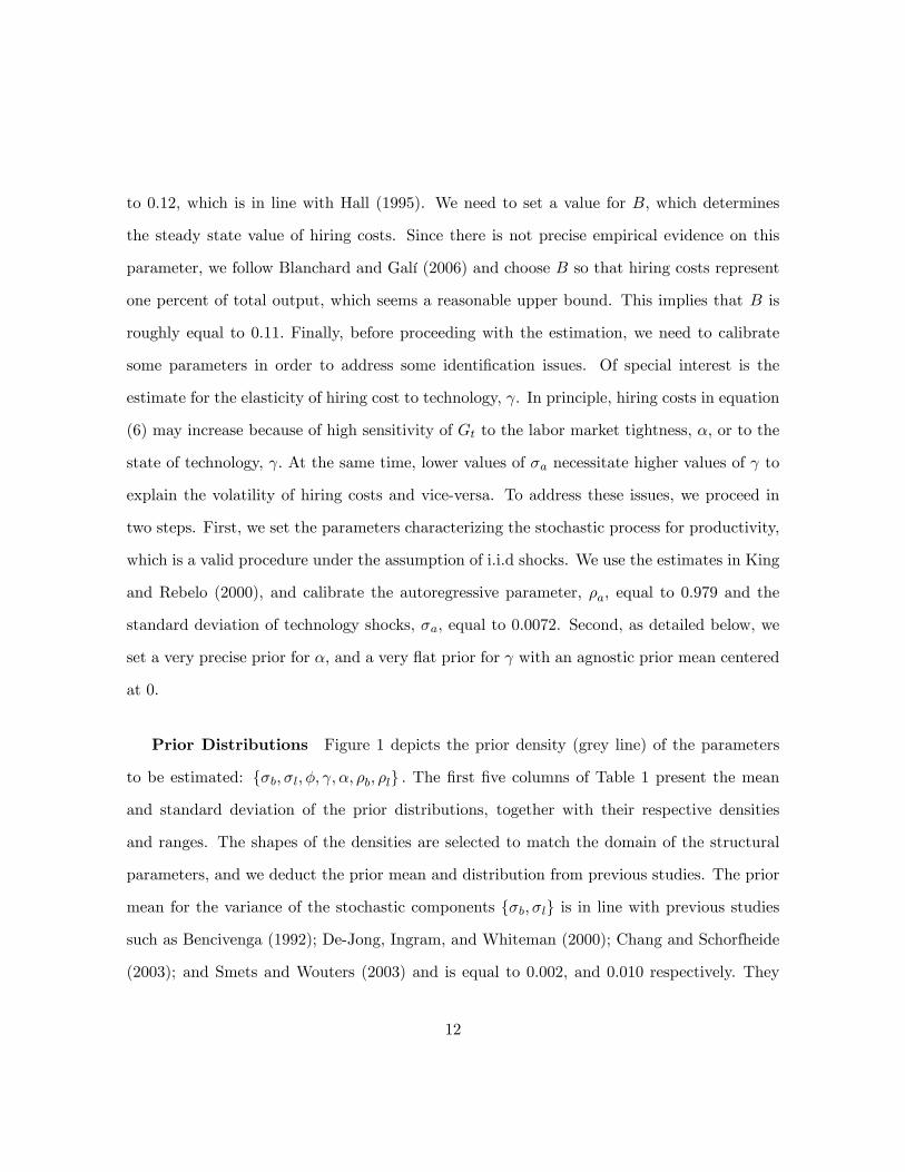
to 0.12, which is in line with Hall (1995). We need to set a value for B; which determines

the steady state value of hiring costs. Since there is not precise empirical evidence on this

parameter, we follow Blanchard and Galí (2006) and choose B so that hiring costs represent

one percent of total output, which seems a reasonable upper bound. This implies that B is

roughly equal to 0:11: Finally, before proceeding with the estimation, we need to calibrate

some parameters in order to address some identi�cation issues. Of special interest is the

estimate for the elasticity of hiring cost to technology, . In principle, hiring costs in equation

(6) may increase because of high sensitivity of Gt to the labor market tightness, �, or to the

state of technology, : At the same time, lower values of �a necessitate higher values of to

explain the volatility of hiring costs and vice-versa. To address these issues, we proceed in

two steps. First, we set the parameters characterizing the stochastic process for productivity,

which is a valid procedure under the assumption of i.i.d shocks. We use the estimates in King

and Rebelo (2000), and calibrate the autoregressive parameter, �a, equal to 0.979 and the

standard deviation of technology shocks, �a, equal to 0.0072. Second, as detailed below, we

set a very precise prior for �, and a very �at prior for with an agnostic prior mean centered

at 0.

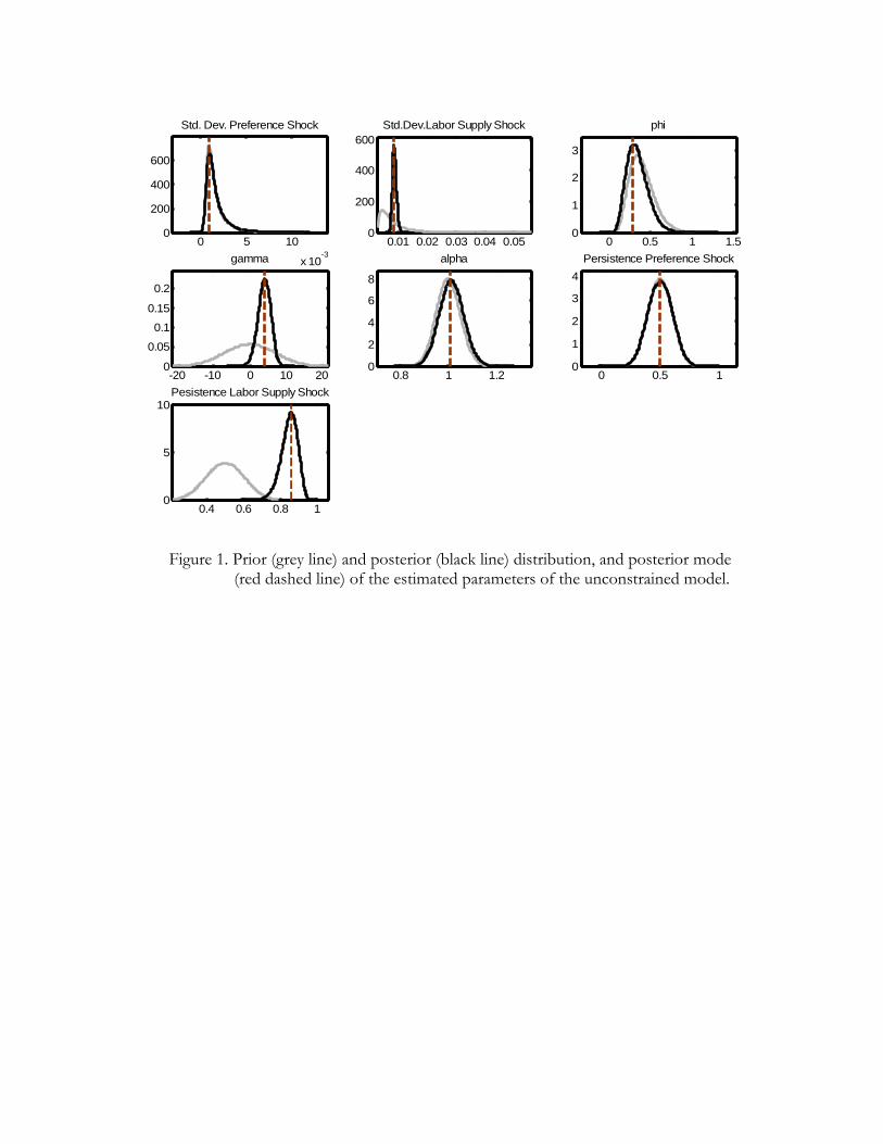
Prior Distributions Figure 1 depicts the prior density (grey line) of the parameters

to be estimated: f�b; �l; �; ; �; �b; �lg : The �rst �ve columns of Table 1 present the mean

and standard deviation of the prior distributions, together with their respective densities

and ranges. The shapes of the densities are selected to match the domain of the structural

parameters, and we deduct the prior mean and distribution from previous studies. The prior

mean for the variance of the stochastic components f�b; �lg is in line with previous studies

such as Bencivenga (1992); De-Jong, Ingram, and Whiteman (2000); Chang and Schorfheide

(2003); and Smets and Wouters (2003) and is equal to 0:002, and 0:010 respectively. They

12

are assumed to have an Inverse Gamma distribution with a degree of freedom equal to 2.

We use this distribution because it delivers positive values with a rather large domain. The

prior distribution of the autoregressive parameters of the shocks is a Beta distribution that

covers the range between 0 and 1, in accordance to the model speci�cation. As is common

practice in the Bayesian estimation literature, we want to distinguish between persistent and

non-persistent shocks, so we choose a precise mean, that is, a rather strict standard error,

which is equal to 0.1. Since the inverse of the Frisch intertemporal elasticity of substitution in

labor supply, �, and the elasticity of labor market tightness with respect to hiring costs, �, are

theoretically restricted to be positive, we consider a Gamma distribution for them. The prior

for � is loosely centered at 0:4 which corresponds to a value in between the microeconomic

estimates, as in Pencavel (1986), and the relative large values usually observed in the macro

literature, as in Rogerson and Wallenius (2007). In setting the prior for �; as suggested

in Blanchard and Galí (2006), we exploit a simple mapping between this model and the

Diamond-Mortensen-Pissarides speci�cation, and assume a precise prior mean equal to 1

with a standard error equal to 0:05; which is su¢ cient to capture the range of estimates in

the literature.8 Finally, since the elasticity of technology shocks to hiring costs, , is allowed

to be either positive, negative, or zero, we assume it has a Normal distribution. In order to

get a reliable identi�cation of , and allow for a wide range of possible values, we impose a

very �at prior with a mean equal to 0 and a standard deviation equal to 7.9

8 In the Diamond-Mortensen-Pissarides speci�cation the expected cost per hire is proportional to the ex-pected duration of a vacancy, with a steady-state value equal to V=H in which V denotes vacancies. Assuminga matching function H = ZU�V 1��: Hence, � in our paper corresponds to �=(1� �) in their setup. Since theestimates of � are typically very close to 0.5, as surveyed in Petrongolo and Pissarides (2001), we assume aprior mean for � equal to one, which is also the parameter value used in Blanchard and Galí (2006).

9To check the robustness of the results to the assumptions on the prior distribution of , we have estimatedthe model using di¤erent means and standard deviations on the prior of this parameter. This has very littleimpact on the results, which are available upon request.

13

Estimation results (posterior distributions) Figure 1 shows the posterior density

(black line) together with the mode of the posterior density (red dotted line) of the estimated

parameters. The plots show that the marginal posteriors and the priors of the behavioral

parameters are di¤erent, supporting the presumption that the data are relatively informative

about the values of the estimated parameters. The last three columns of Table 1 report

the posterior mean and 95% probability interval of the structural parameters. The posterior

mean of the inverse of the Frisch intertemporal elasticity of substitution in labor supply, �,

equals to 0.34, which implies an elasticity of labor supply equal to 2.9. This is consistent

with the value suggested by Rogerson and Wallenius (2007) and more generally is in line

with the calibrated values used in the macro literature as advocated by King and Rebelo

(2000). The posterior mean of the elasticity of hiring costs to labor market tightness, �, is

1.01. As shown in Blanchard and Galí (2006), in a decentralized version of this economy, we

can interpret this parameter as the ratio between the wage bargaining power of households

and �rms. Therefore, the estimated unitary value supports the idea that households and

�rms share their bargaining power equally. This result is in line with the empirical �ndings in

Petrongolo and Pissarides (2001). Of special interest here, of course, is the estimate for the

elasticity of hiring costs to technology, . The posterior mean of is 4.00, which, as detailed

below, supports the fact that the data prefer a positive response of hiring costs to technology

shocks. In addition, notice that the estimation delivers a sizable reading for despite its

loose prior.

Turning now to the stochastic processes, the posterior mean of the persistence of preference

shocks, �b, is 0.50, while the estimate of the persistence of labor supply shocks, �l, is 0.85.

The posterior mean of the volatility of preference shocks, �b, is 0.0018, and the posterior

mean of the volatility of labor supply shocks, �l, is 0.0087. These values are similar to the

estimates in Smets and Wouters (2003, 2007), and Chang, Doh, and Schorfheide (2007).

14

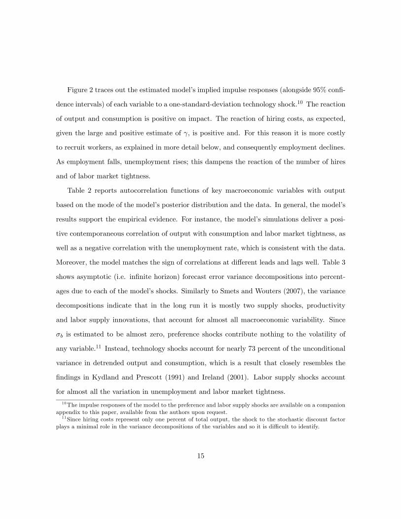
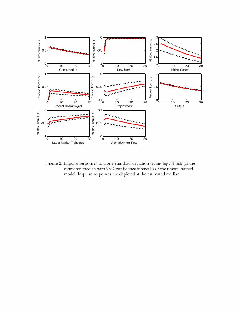
Figure 2 traces out the estimated model�s implied impulse responses (alongside 95% con�-

dence intervals) of each variable to a one-standard-deviation technology shock.10 The reaction

of output and consumption is positive on impact. The reaction of hiring costs, as expected,

given the large and positive estimate of , is positive and. For this reason it is more costly

to recruit workers, as explained in more detail below, and consequently employment declines.

As employment falls, unemployment rises; this dampens the reaction of the number of hires

and of labor market tightness.

Table 2 reports autocorrelation functions of key macroeconomic variables with output

based on the mode of the model�s posterior distribution and the data. In general, the model�s

results support the empirical evidence. For instance, the model�s simulations deliver a posi-

tive contemporaneous correlation of output with consumption and labor market tightness, as

well as a negative correlation with the unemployment rate, which is consistent with the data.

Moreover, the model matches the sign of correlations at di¤erent leads and lags well. Table 3

shows asymptotic (i.e. in�nite horizon) forecast error variance decompositions into percent-

ages due to each of the model�s shocks. Similarly to Smets and Wouters (2007), the variance

decompositions indicate that in the long run it is mostly two supply shocks, productivity

and labor supply innovations, that account for almost all macroeconomic variability. Since

�b is estimated to be almost zero, preference shocks contribute nothing to the volatility of

any variable.11 Instead, technology shocks account for nearly 73 percent of the unconditional

variance in detrended output and consumption, which is a result that closely resembles the

�ndings in Kydland and Prescott (1991) and Ireland (2001). Labor supply shocks account

for almost all the variation in unemployment and labor market tightness.

10The impulse responses of the model to the preference and labor supply shocks are available on a companionappendix to this paper, available from the authors upon request.11Since hiring costs represent only one percent of total output, the shock to the stochastic discount factor

plays a minimal role in the variance decompositions of the variables and so it is di¢ cult to identify.

15

4 The Role of Labor Market Frictions

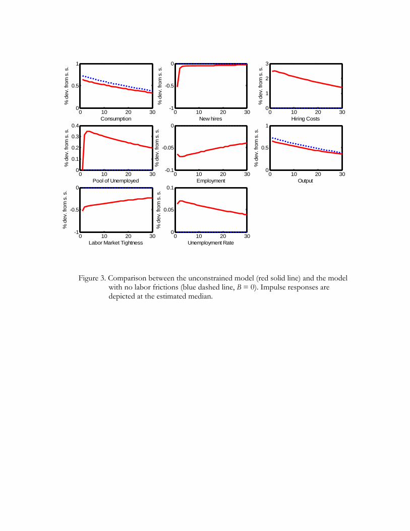
No hiring costs In order to establish a benchmark against which to compare, Table

4 estimates the model imposing B = 0, so that the theoretical framework nests the �rst

order conditions of a standard RBC model where labor frictions are absent. To be consistent

throughout the estimation exercise, the prior distributions of the parameters are the same as

those in the baseline model. Estimation results indicate that the posterior mean of the inverse

of the elasticity of labor supply, �, equals 0.39, and the posterior mean of the autoregressive

component of the labor supply shocks is highly persistent. Similarly, the magnitude of the

volatility of the shocks is close to that of the unconstrained model. In general, these estimates

are similar to those in the model that allow for labor market frictions, and, moreover, are

in line with �ndings in Bencivenga (1992); De-Jong, Ingram, and Whiteman (2000); Ireland

(2001, 2004); Chang and Schorfheide (2003); and Zanetti (2007) who estimate standard RBC

models.

What lies behind the posterior means of the parameters for the reaction of the variables

to technology shocks? Figure 3 traces out the estimated model�s implied impulse responses

of each variable to a one-standard-deviation technology shock for both versions of the model,

with and without labor frictions. It is immediately noticeable that the reaction of output

and consumption is quantitatively the same across the two models, while the reaction of

employment is negative in the presence of labor market frictions.12

How can the presence of labor market frictions generate such a striking result? As men-

tioned, the answer lies in the way hiring costs react to productivity shocks. Here the reaction

is determined by the elasticity of hiring costs to a technology shock, which is represented

by the parameter . The estimation exercise allows the value of this parameter to be either

12Of course, in the model with labor market frictions, in addition to the reaction of output, consumption,employment, we can also trace out the dynamics of �ring costs, number of hirings, and labor market tightness.

16

positive, negative, or equal to zero and leaves the data to choose the preferred value. The

estimation suggests that the data prefer to be positive, such that hiring costs co-move

positively with technology shocks (which is also the assumption in the calibrated model of

Blanchard and Galí (2006)). To understand how this generates a negative reaction of em-

ployment to technology shocks, consider equation (11), which represents the labor market

equilibrium condition. A productivity shock would increase the marginal product of labor,

the �rst term on the right hand side of equation (11), as in the standard RBC model, but

it would also increase the cost of recruiting an additional worker, the second term on the

right hand side of equation (11), and, at the same time, reduce the hiring needs in period

t+ 1, the third term on the right hand side of equation (11). The e¤ect on the second term,

namely the cost of recruiting an additional worker, dominates the other two and, as a re-

sult, the marginal rate of transformation, which is the right hand side of equation (11) is

reduced, and therefore generate a negative response of employment to technology shocks. In

the standard RBC model, the correspondent equilibrium condition, equivalent to equation

(11), is "ltN�+1t ="bt = 1, which implies a level of employment invariant to technology shocks,

which is the result of o¤setting income and substitution e¤ects on labor supply. Without

capital accumulation, such a result is standard in this class of models, as King and Rebelo

(2000) point out. Despite the di¤erent reactions of employment to a technology shock, the

functioning of the two models is qualitatively similar.

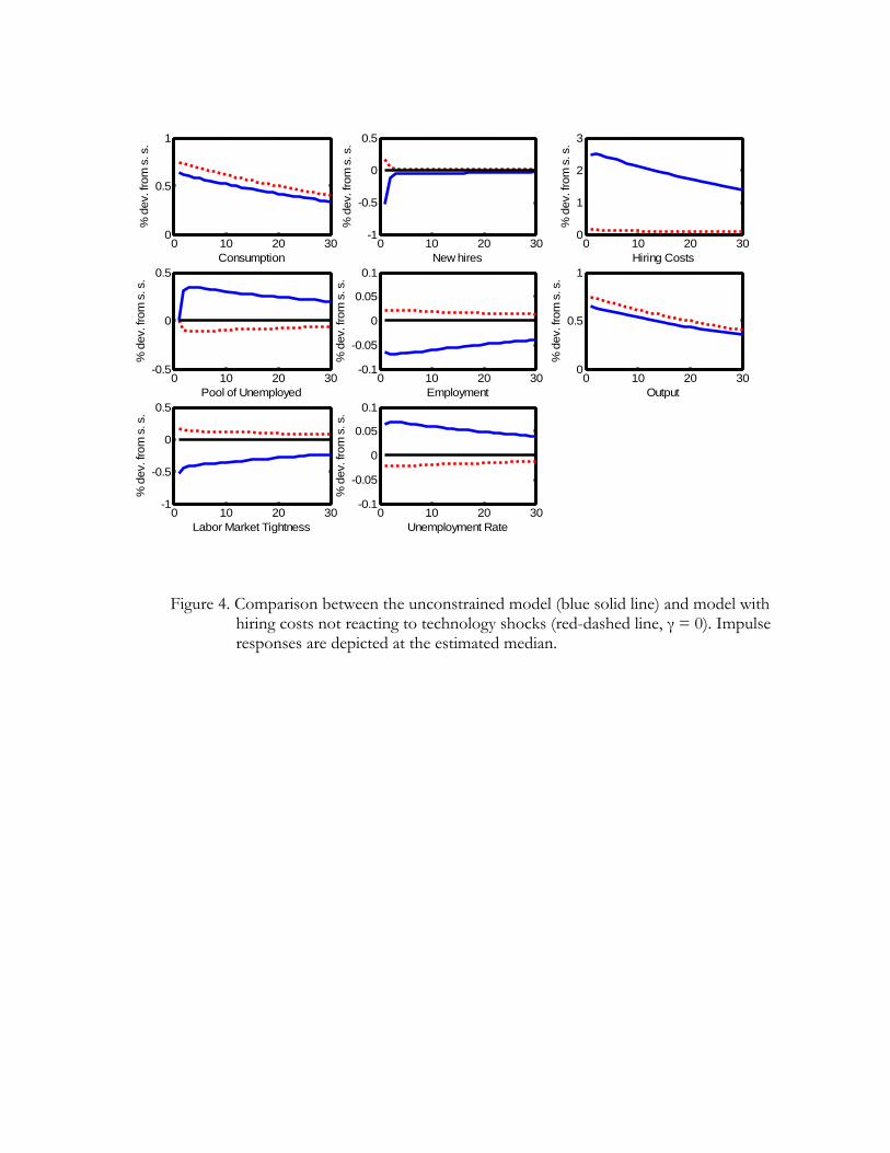
Hiring costs not reactive to technological shocks Turning to the parameter de-

scribing the elasticity of hiring costs to technology shocks, , we now impose the neutral

assumption that hiring costs do not react directly to technology shocks. In this way, we

determine whether the data prefer the version of the model with hiring costs reacting to

technology shocks or a more constrained speci�cation where hiring costs do not directly react

17

to technology. We test which version of the model the data prefer by imposing = 0 on

the speci�cation of the model. As before, the prior distributions of the parameters are the

same as those in the baseline model. Table 4 reports the posterior mean and 95% probability

interval of the parameters for the constrained model. The posterior mean of the structural

parameters for this constrained speci�cation are reasonably close to those where is allowed

to di¤er from zero. In particular, the posterior mean of the inverse of the elasticity of labor

supply, �, equals 0.34, and the posterior mean of the autoregressive component of the labor

supply shocks are highly persistent. Results indicate that the volatility of the stochastic com-

ponents are of a similar magnitude than the estimates of the unconstrained model. Also in

this instance, the posterior mean of � is almost unitary and equals 1.01. Overall, the similar-

ity of these estimates with those described above suggests that the underlying RBC model

is consistently estimated across di¤erent model speci�cations. Figure 4 shows the model�s

implied impulse responses of each variable to a one-standard-deviation technology shock for

both the constrained model where = 0, and the RBC model with labor frictions. Output,

consumption, and employment positively react to a technology shock, as in the unconstrained

speci�cation. When = 0; hiring costs do not directly react to technological innovations. In

this case, the e¤ect on the second term on the right hand side of equation (11), namely the

cost of recruiting an additional worker, is dominated by the counteracting e¤ect of the two

other terms, thus generating a positive response of employment to technology shocks. The

positive reaction of employment leads to a positive response in the number of hires and this,

coupled with the negative reaction of unemployment, generates an increase in labor market

tightness and, consequently, the cost of hiring increases slightly on impact.

Model Comparison In order to establish whether the data prefer the unconstrained

formulation of the model, the version without labor market frictions (B = 0); or the version

18

in which hiring costs do not directly react to technological innovations ( = 0), we �rst

consider the di¤erence between the log marginal likelihood of each model with respect to

the log marginal likelihood of the unconstrained speci�cation. We thus de�ne the marginal

likelihood of a model, J , as follows: MJ =R� P (�jJ)P (Z

T j�; J)d�: Where P (�jJ) is the

prior density for model J , and P (ZT j�; J) is the likelihood function of the observable data,

conditional on the parameter space � and the model J . The marginal likelihood of a model

(or the Bayes factor) is directly related to the predicted density of the model given by:

p̂T+mT+1 =R� P (�jZ

T ; J)T+m�

t=T+1P (ztjZT ;�; J)d�: Therefore the marginal likelihood of a model

also re�ects its prediction performance.

Considering that this criterion penalizes overparametrization, models with labor market

frictions do not necessarily rank better if the extra friction does not su¢ ciently help in ex-

plaining the data. As from the last row of Table 4, the log marginal likelihood di¤erence

between the unconstrained speci�cation and the model with no hiring costs is 24.53. In other

words, in order to choose the constrained version over the original formulation, the Bayes

factor requires a prior probability over the constrained version e24:53 times larger than over

the unconstrained model. This can be accepted as conclusive evidence in favor of the model

with labor market frictions, as suggested in Rabanal and Rubio-Ramírez (2005). Refering to

the last row of Table 4, the data also prefer the unconstrained version of the model in which

estimation results re�ect hiring costs that respond pro-cyclically to technology shocks. In

fact, the log-di¤erence between the unconstrained speci�cation and the one in which = 0;

is 1.11.

As a �nal exercise, in line with the RBC tradition and the seminal work by Merz (1995),

we determine which version of the model better matches the sample statistics in the data.

Here the series are treated in the same way as in the estimation exercise. Table 5 reports

measures of volatility for the posterior means relative to output for the series of consumption,

19

Ct, and the unemployment rate, ut, in the di¤erent models and the data. The model with

labor market frictions produces relative standard deviations of the unemployment rate and

consumption that are closer to the values in the data, than the model without labor frictions.

Overall, the match between models with labor market frictions and data is better than that

of alternative speci�cations. In the models characterized by labor market frictions, as in

the data, consumption is always less volatile than output, and the unemployment rate is less

volatile than both output and consumption. The ability of the model to replicate the moments

in the data could improve if capital accumulation is added into the model�s speci�cation. In

fact, as pointed out in King and Rebelo (2000), the presence of capital accumulation is central

for the RBC framework to match the cyclical movements that we see in the data. In this

study, the model excludes capital in order to maintain the theoretical framework as close

as possible to that of Blanchard and Galí (2006) and leave the investigation of the e¤ect of

capital open for future research.

5 Conclusion

Recent empirical evidence led by Galí (1999) and supported by several other studies suggests

that a positive technology shock leads to a decline in labor inputs. This is the opposite of a

key prediction of the standard RBC model, thereby calling the validity of the RBC paradigm

into question. This paper has investigated whether the presence of labor market frictions,

which are modeled as in Blanchard and Galí (2006), may rehabilitate the RBC framework.

Using Bayesian techniques, we show that data support the presence of labor market frictions

as the factor responsible for the negative response of employment to a technology shock.

The �ndings of this paper support those who suggest that it seems premature to reject

the notion that technology shocks are the main driving forces of the business cycle on the

20

ground of the negative response of employment to technology shocks.

6 References

Alexopoulos, M. (2006). �Read all about it! What happens after a technology shock�,Department of Economics University of Toronto.

Basu, S., Fernald J. G. and Kimball, M. S. (2006). �Are technology improvements contrac-tionary?�, American Economic Review, vol. 96(5) (December), pp. 1418-48.

Bean, C. R. (1994). �European unemployment: a survey�, Journal of Economic Literature,vol. 32(2) (June), pp. 573-619.

Bencivenga, V. R. (1992). �An econometric study of hours and output variation with pref-erence shocks�, International Economic Review, vol. 33(2) (May), pp. 449-71.

Blanchard, O. J. and Galí, J. (2006). �A new Keynesian model with unemployment�, Re-search Series 200610-4, National Bank of Belgium.

Blanchard, O. J. and Khan, C. M. (1980). �The solution of linear di¤erence models underrational expectation�, Econometrica, vol. 48 (5) (July), pp. 1305-11.

Canova, F., López-Salido, D. and Michelacci, C. (2007). �The labor market e¤ects of tech-nology shocks�, Documentos de trabajo 0719, Banco de España.

Chang, Y., Doh, T. and Schorfheide, F. (2007). �Non-stationary hours in a DSGE model�,Journal of Money, Credit, and Banking, vol. 39(6) (September), pp. 1357-73.

Chang, Y. and Schorfheide, F. (2003). �Labor-supply shifts and economic �uctuations�,Journal of Monetary Economics, vol. 50(8) (November), pp. 1751-68.

Chari, V. V., Kehoe P. J. and McGrattan, E. (2005). �A critique of structural VARs usingbusiness cycle theory�, Research Department Sta¤ Report 364. Minneapolis: FederalReserve Bank of Minneapolis.

Christiano, L. J., Eichenbaum, M. and Vigfusson, R. (2004). �The response of hours toa technology shock: evidence based on direct measures of technology�, Journal of theEuropean Economic Association, vol. 2(2-3) (April-May), pp. 381-95.

Collard, F. and Dellas, H. (2007). �Technology shocks and employment�, Economic Journal,vol. 117, pp. 1436-59.

De-Jong, D. N., Ingram, B. F. and Whiteman, C. H. (2000). �Keynesian impulses versusSolow residuals: identifying sources of business cycle �uctuations�, Journal of AppliedEconometrics, vol. 15(3) (May/June), pp. 311-29.

21

Fernandez-Villaverde, J. and Rubio-Ramírez, J. (2004). �Comparing dynamic equilibriumeconomies to data: a Bayesian approach�, Journal of Econometrics, vol. 123(1) (Janu-ary), pp 153-87.

Francis, N. and Ramey, V. A. (2005). �Is the technology-driven real business cycle hypothesisdead? Shocks and aggregate �uctuations revisited�, Journal of Monetary Economics,vol. 52(8) (November), pp. 1379-99.

Galí, J. (1999). �Technology, employment, and the business cycle: do technology shocksexplain aggregate �uctuations?�, American Economic Review, vol. 89(1) (March), pages249-71.

Hairault, J-O., Langot, F. and Portier, F. (1997). �Time to implement and aggregate �uc-tuations�, Journal of Economic Dynamics and Control, vol. 22(1) (November), pp.109-21.

Hall, R. E. (1995). �Lost Jobs�, Brookings Papers on Economic Activity, vol. 1, pp. 221-56.

Ireland, P. N. (2001). �Technology shocks and the business cycle: an empirical investigation�,Journal of Economic Dynamics and Control, vol. 25(5) (May), pp. 703-19.

Ireland, P. N. (2004). �A method for taking models to the data�, Journal of EconomicDynamics and Control, vol. 28(6) (March), pp. 1205-26.

King, R. and Rebelo, S. (2000). �Resuscitating real business cycle�, in (Taylor, J. B. andWoodford, M., eds.), Handbook of Macroeconomics, Amsterdam: North Holland.

Klein, P. (2000). �Using the generalized Schur form to solve a multivariate linear rationalexpectations model�, Journal of Economic Dynamics and Control, vol. 24(10) (Septem-ber), pp. 1405-23.

Kydland, F. E. and Prescott, E. C. (1982). �Time to build and aggregate �uctuations�,Econometrica, vol. 50(6) (November), pp. 1345-70.

Kydland, F. E. and Prescott, E. C. (1991). �Hours and employment variation in businesscycle theory�, Economic Theory, vol. 1(1) (January), pp. 63-81.

Leeper E. M. and Zha, T. (2000). �Assessing simple policy rules: a view from a completemacro model�, Working Paper 2000-19, Federal Reserve Bank of Atlanta.

Liu, Z. and Phaneuf, L. (2007). �Technology shocks and labor market dynamics: someevidence and theory�, Journal of Monetary Economics, forthcoming.

Lindé, J. (2004). �The e¤ects of permanent technology shocks on labor productivity andhours in the RBC model�, Working Paper Series 161, Sveriges Riksbank.

22

López-Salido, D. and Michelacci, C. (2007). �Technology shocks and job �ows�, Review ofEconomic Studies, forthcoming.

Lubik, T. and Schorfheide, F. (2005). �A Bayesian look at new open economy macroeco-nomics�, NBER Macroeconomics Annual, pp. 313-66.

Merz, M. (1995). �Search in the labor market and the real business cycle�, Journal ofMonetary Economics, vol. 36(2) (November), pp. 269-300.

McGrattan, E. (2004). �Comment on Galí and Rabanal�s Technology shocks and aggregate�uctuations: how well does the RBC model �t postwar U.S. data?�, NBER Macroeco-nomics Annual, pp. 289-308.

Nickell, S. (1997). �Unemployment and labor market rigidities: Europe versus North Amer-ica�, The Journal of Economic Perspectives, vol. 11(3) (Summer), pp. 55-74.

Pencavel, J. (1986). �Labor supply of men: a survey�, in (Ashenfelter, O. and Layard, R.,eds.), Handbook of Labor Economics, Amsterdam: North Holland.

Petrongolo, B. and Pissarides, C. (2001). �Looking into the black box: a survey of thematching function�, Journal of Economic Literature, vol. 38(2) (June), pp. 390-431.

Rabanal, P. and Rubio-Ramírez, J. F. (2005). �Comparing new Keynesian models of thebusiness cycle: a Bayesian approach�, Journal of Monetary Economics, vol. 52(6) (Sep-tember), pp. 1151-66.

Rogerson, R. and Wallenius, J. (2007). �Micro and macro elasticities in a life cycle modelwith taxes�, NBER Working Paper No. 13017.

Rotemberg, J. J. (2006). �Cyclical wages in a search-and-bargaining model with large �rms�,NBER Working Paper No. 12415.

Shea, J. S. (1998). �What do technology shocks do?�NBER Working Paper No. 6632.

Shimer, R. (2007). �Reassessing the ins and outs of unemployment�, NBER Working PaperNo. 13421.

Smets, F. and Wouters, R. (2003). �An estimated dynamic stochastic general equilibriummodel of the euro area�, Journal of the European Economic Association, vol. 1(5)(September), pp. 1123-75.

Smets, F. and Wouters, R. (2007). �Shocks and frictions in US business cycles: a BayesianDSGE approach�, American Economic Review, vol. 97(3) (June), pp. 586-606.

Wang, P. and Wen, Y. (2007). �Understanding the puzzling e¤ects of technology shocks�,Working Papers 2007-018, Federal Reserve Bank of St. Louis.

23

Whelan, K. (2004). �Technology shocks and hours worked: checking for robust conclusions�,Central Bank and Financial Services Authority of Ireland Research Technical Paper No.6/RT/04.

Yashiv, E. (2000a). �Hiring as investment behavior�, Review of Economic Dynamics, vol.3(3) (July), pp. 486-522.

Yashiv, E. (2000b). �The determinants of equilibrium unemployment�, American EconomicReview, vol. 90(5) (December), pp. 1297-1322.

Yashiv, E. (2006). �Evaluating the performance of the search and matching model�, EuropeanEconomic Review, vol. 50(4) (May), pp. 909-36.

Yashiv, E. (2007). �Labor search and matching in macroeconomics�, European EconomicReview, forthcoming.

Zanetti, F. (2007). �Labor and investment frictions in the real business cycle model�, Bankof England, unpublished manuscript.

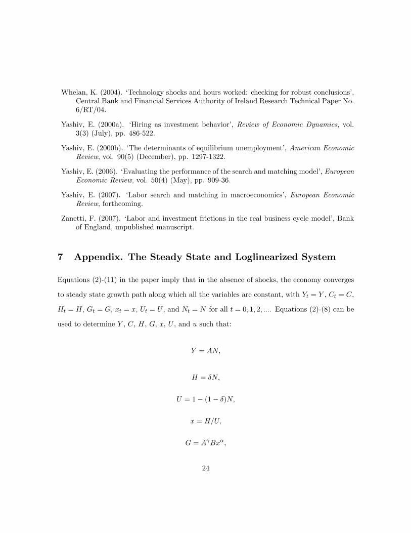
7 Appendix. The Steady State and Loglinearized System

Equations (2)-(11) in the paper imply that in the absence of shocks, the economy converges

to steady state growth path along which all the variables are constant, with Yt = Y , Ct = C,

Ht = H, Gt = G, xt = x, Ut = U , and Nt = N for all t = 0; 1; 2; :::. Equations (2)-(8) can be

used to determine Y , C, H, G, x, U , and u such that:

Y = AN;

H = �N;

U = 1� (1� �)N;

x = H=U;

G = A Bx�;

24

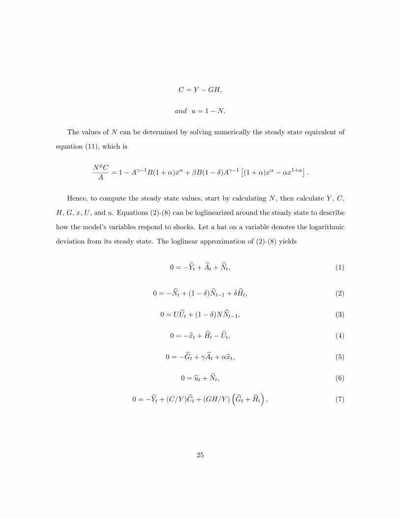
C = Y �GH;

and u = 1�N:

The values of N can be determined by solving numerically the steady state equivalent of

equation (11), which is

N�C

A= 1�A �1B(1 + �)x� + �B(1� �)A �1

�(1 + �)x� � �x1+�

�:

Hence, to compute the steady state values, start by calculating N , then calculate Y , C,

H, G, x, U , and u. Equations (2)-(8) can be loglinearized around the steady state to describe

how the model�s variables respond to shocks. Let a hat on a variable denotes the logarithmic

deviation from its steady state. The loglinear approximation of (2)-(8) yields

0 = �bYt + bAt + bNt; (1)

0 = � bNt + (1� �) bNt�1 + � bHt; (2)

0 = U bUt + (1� �)N bNt�1; (3)

0 = �bxt + bHt � bUt; (4)

0 = � bGt + bAt + �bxt; (5)

0 = but + bNt; (6)

0 = �bYt + (C=Y ) bCt + (GH=Y )� bGt + bHt� ; (7)

25

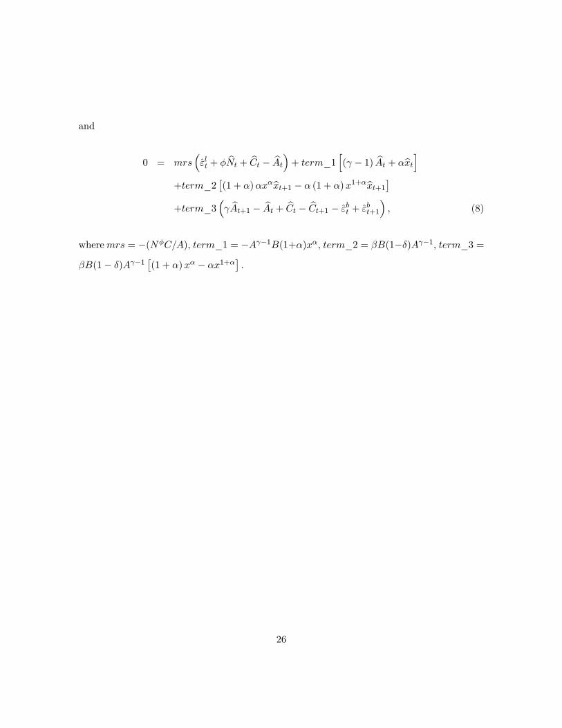
and

0 = mrs�"̂lt + � bNt + bCt � bAt�+ term_1 h( � 1) bAt + �bxti

+term_2�(1 + �)�x�bxt+1 � � (1 + �)x1+�bxt+1�

+term_3� bAt+1 � bAt + bCt � bCt+1 � "̂bt + "̂bt+1� ; (8)

wheremrs = �(N�C=A), term_1 = �A �1B(1+�)x�, term_2 = �B(1��)A �1, term_3 =

�B(1� �)A �1�(1 + �)x� � �x1+�

�:

26

Table 1. Summary statistics for the prior and posterior distribution of the

parameters

Parameter Prior Mean Prior SE Density Range Posterior 2.5% 97.5%

� 0.40 0.15 Gamma R+ 0.3438 0.1322 0.5367

0 7 Normal R 4.0003 1.1526 6.873

� 1 0.05 Gamma R+ 1.0126 0.9303 1.0947

�b 0.5 0.1 Beta [0,1] 0.5005 0.3306 0.6603

�l 0.5 0.1 Beta [0,1] 0.8485 0.7801 0.9214

�b 0.002 2* Inv gamma R+ 0.0018 0.0005 0.0033

�l 0.01 2* Inv gamma R+ 0.0087 0.0076 0.0099

Notes: Results based on 200,000 draws of the Metropolis Algorithm. For the Inverted Gamma function

the degrees of freedom are indicated.

27

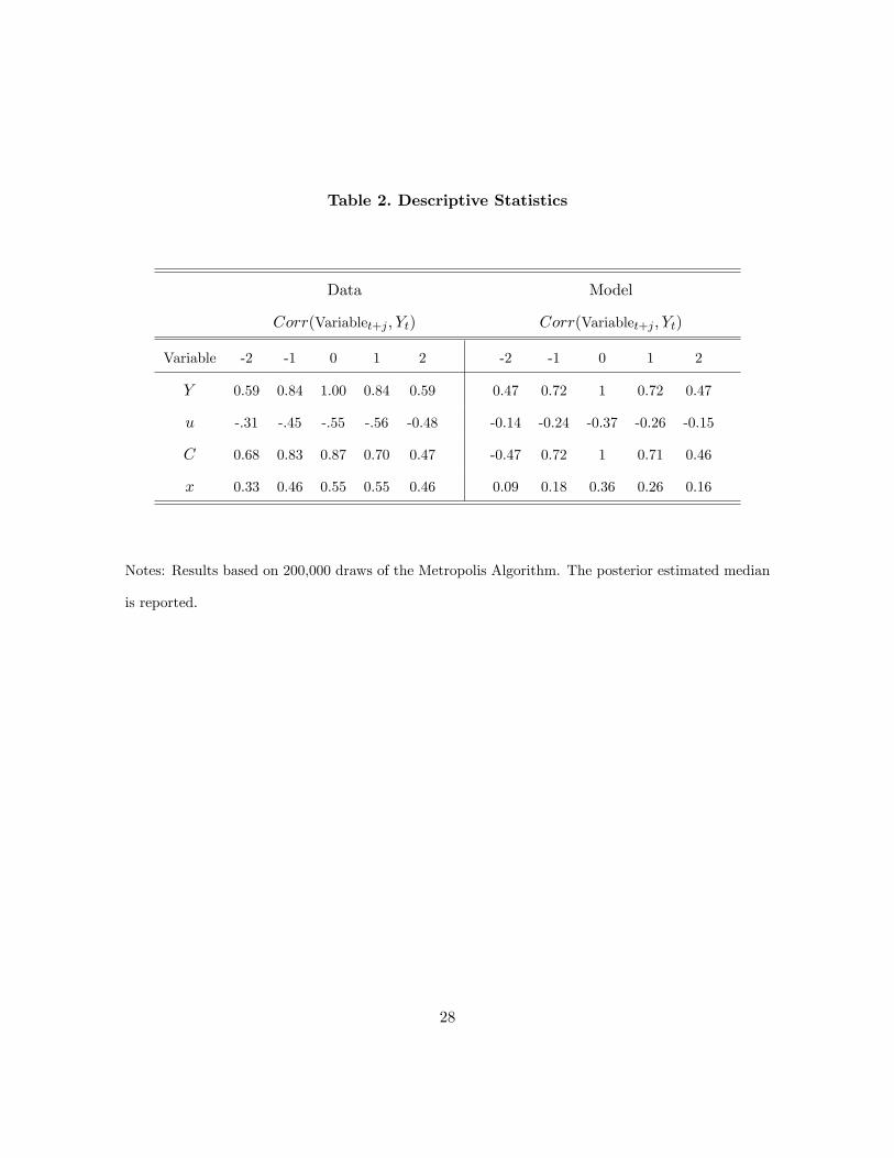
Table 2. Descriptive Statistics

Data Model

Corr(Variablet+j ; Yt) Corr(Variablet+j ; Yt)

Variable -2 -1 0 1 2 -2 -1 0 1 2

Y 0.59 0.84 1.00 0.84 0.59 0.47 0.72 1 0.72 0.47

u -.31 -.45 -.55 -.56 -0.48 -0.14 -0.24 -0.37 -0.26 -0.15

C 0.68 0.83 0.87 0.70 0.47 -0.47 0.72 1 0.71 0.46

x 0.33 0.46 0.55 0.55 0.46 0.09 0.18 0.36 0.26 0.16

Notes: Results based on 200,000 draws of the Metropolis Algorithm. The posterior estimated median

is reported.

28

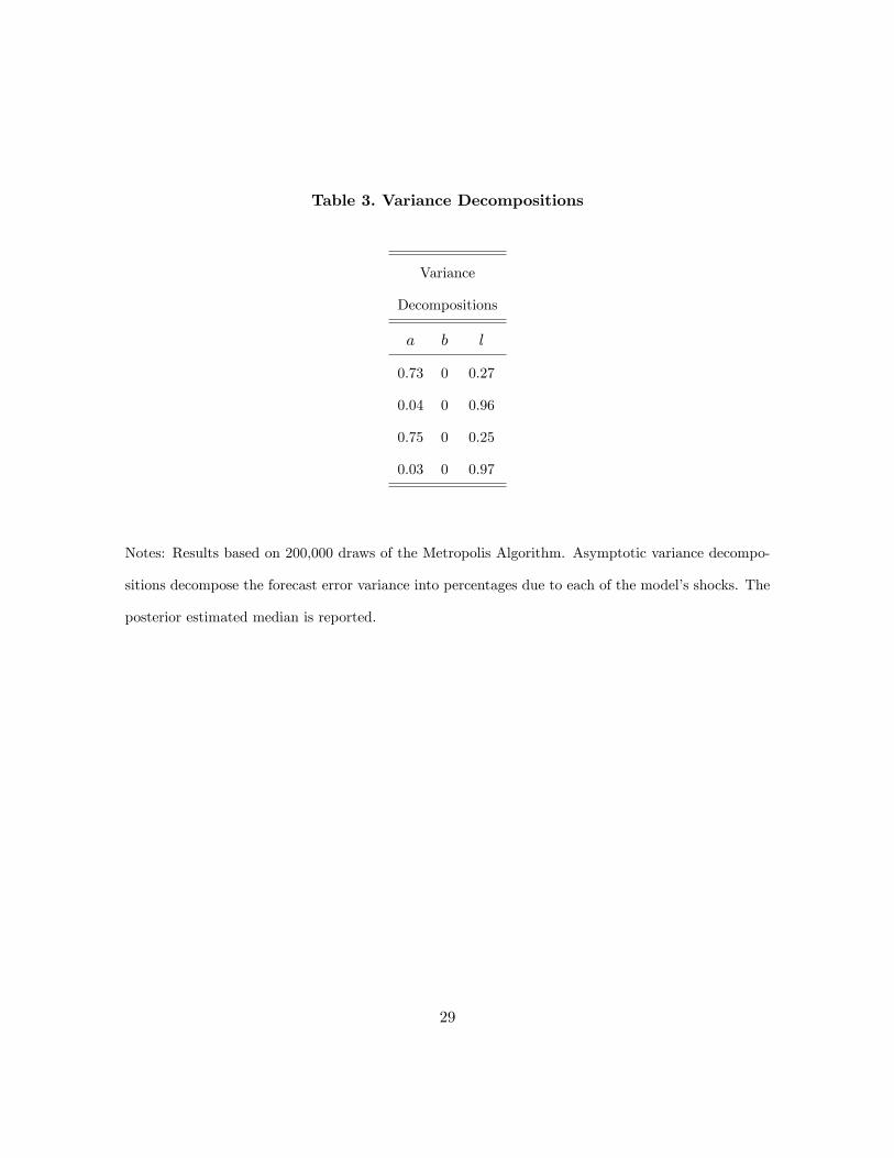
Table 3. Variance Decompositions

Variance

Decompositions

a b l

0.73 0 0.27

0.04 0 0.96

0.75 0 0.25

0.03 0 0.97

Notes: Results based on 200,000 draws of the Metropolis Algorithm. Asymptotic variance decompo-

sitions decompose the forecast error variance into percentages due to each of the model�s shocks. The

posterior estimated median is reported.

29

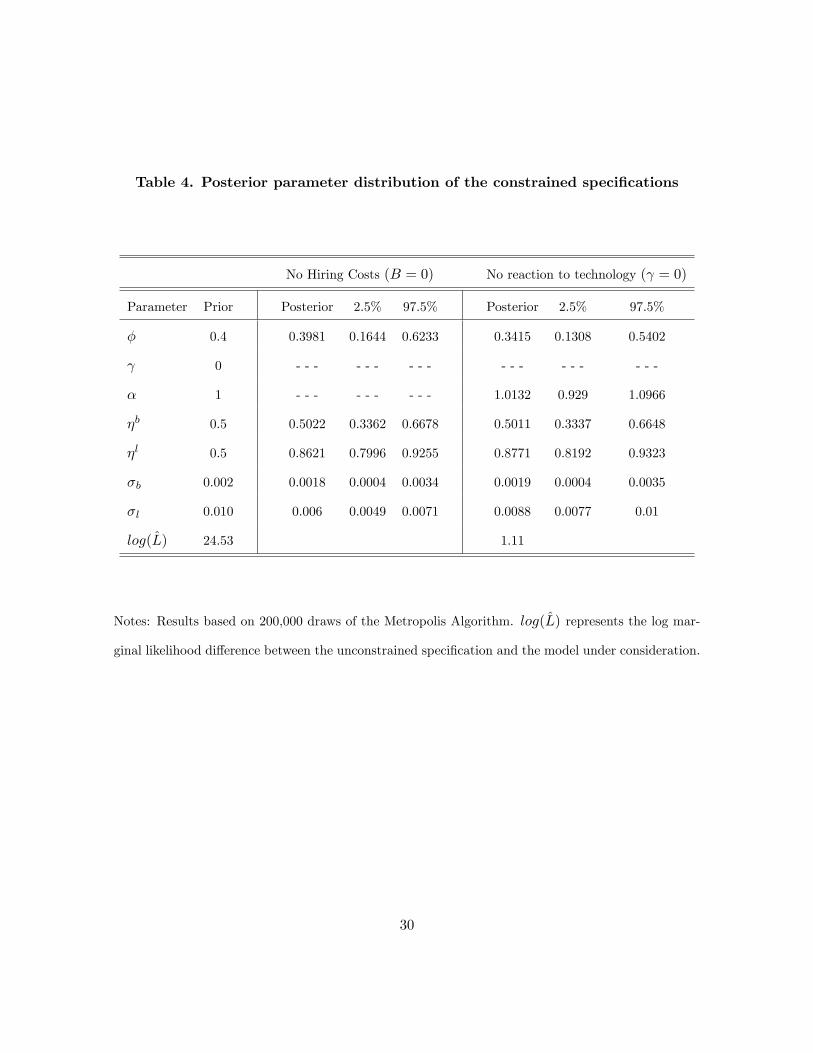
Table 4. Posterior parameter distribution of the constrained speci�cations

No Hiring Costs (B = 0) No reaction to technology ( = 0)

Parameter Prior Posterior 2.5% 97.5% Posterior 2.5% 97.5%

� 0.4 0.3981 0.1644 0.6233 0.3415 0.1308 0.5402

0 - - - - - - - - - - - - - - - - - -

� 1 - - - - - - - - - 1.0132 0.929 1.0966

�b 0.5 0.5022 0.3362 0.6678 0.5011 0.3337 0.6648

�l 0.5 0.8621 0.7996 0.9255 0.8771 0.8192 0.9323

�b 0.002 0.0018 0.0004 0.0034 0.0019 0.0004 0.0035

�l 0.010 0.006 0.0049 0.0071 0.0088 0.0077 0.01

log(L̂) 24.53 1.11

Notes: Results based on 200,000 draws of the Metropolis Algorithm. log(L̂) represents the log mar-

ginal likelihood di¤erence between the unconstrained speci�cation and the model under consideration.

30

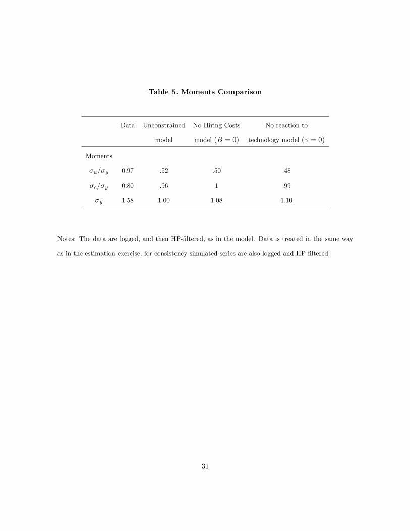
Table 5. Moments Comparison

Data Unconstrained No Hiring Costs No reaction to

model model (B = 0) technology model ( = 0)

Moments

�u=�y 0.97 .52 .50 .48

�c=�y 0.80 .96 1 .99

�y 1.58 1.00 1.08 1.10

Notes: The data are logged, and then HP-�ltered, as in the model. Data is treated in the same way

as in the estimation exercise, for consistency simulated series are also logged and HP-�ltered.

31

0 5 10

x 10-3

0

200

400

600

Std. Dev. Preference Shock

0.01 0.02 0.03 0.04 0.050

200

400

600Std.Dev.Labor Supply Shock

0 0.5 1 1.50

1

2

3

phi

-20 -10 0 10 200

0.05

0.1

0.15

0.2

gamma

0.8 1 1.20

2

4

6

8

alpha

0 0.5 10

1

2

3

4Persistence Preference Shock

0.4 0.6 0.8 10

5

10Pesistence Labor Supply Shock

Figure 1. Prior (grey line) and posterior (black line) distribution, and posterior mode

(red dashed line) of the estimated parameters of the unconstrained model.

0 10 20 300

0.5

1

Consumption

% d

ev. f

rom

s. s

.

0 10 20 30-1

-0.5

0

New hires

% d

ev. f

rom

s. s

.

0 10 20 301

1.5

2

2.5

3

Hiring Costs

% d

ev. f

rom

s. s

.

0 10 20 300

0.5

1

Pool of Unemployed

% d

ev. f

rom

s. s

.

0 10 20 30-0.1

-0.05

0

Employment

% d

ev. f

rom

s. s

.

0 10 20 300

0.5

1

Output

% d

ev. f

rom

s. s

.

0 10 20 30-1

-0.5

0

Labor Market Tightness

% d

ev. f

rom

s. s

.

0 10 20 300

0.05

0.1

Unemployment Rate

% d

ev. f

rom

s. s

.

Figure 2. Impulse responses to a one-standard-deviation technology shock (at the estimated median with 95% confidence intervals) of the unconstrained model. Impulse responses are depicted at the estimated median.

0 10 20 300

0.5

1

Consumption

% d

ev. f

rom

s. s

.

0 10 20 30-1

-0.5

0

New hires

% d

ev. f

rom

s. s

.

0 10 20 300

1

2

3

Hiring Costs

% d

ev. f

rom

s. s

.

0 10 20 300

0.1

0.2

0.3

0.4

Pool of Unemployed

% d

ev. f

rom

s. s

.

0 10 20 30-0.1

-0.05

0

Employment

% d

ev. f

rom

s. s

.

0 10 20 300

0.5

1

Output

% d

ev. f

rom

s. s

.

0 10 20 30-1

-0.5

0

Labor Market Tightness

% d

ev. f

rom

s. s

.

0 10 20 300

0.05

0.1

Unemployment Rate

% d

ev. f

rom

s. s

.

Figure 3. Comparison between the unconstrained model (red solid line) and the model with no labor frictions (blue dashed line, B = 0). Impulse responses are depicted at the estimated median.

0 10 20 300

0.5

1

Consumption

% d

ev. f

rom

s. s

.

0 10 20 30-1

-0.5

0

0.5

New hires

% d

ev. f

rom

s. s

.

0 10 20 300

1

2

3

Hiring Costs

% d

ev. f

rom

s. s

.

0 10 20 30-0.5

0

0.5

Pool of Unemployed

% d

ev. f

rom

s. s

.

0 10 20 30-0.1

-0.05

0

0.05

0.1

Employment

% d

ev. f

rom

s. s

.

0 10 20 300

0.5

1

Output

% d

ev. f

rom

s. s

.

0 10 20 30-1

-0.5

0

0.5

Labor Market Tightness

% d

ev. f

rom

s. s

.

0 10 20 30-0.1

-0.05

0

0.05

0.1

Unemployment Rate

% d

ev. f

rom

s. s

.

Figure 4. Comparison between the unconstrained model (blue solid line) and model with

hiring costs not reacting to technology shocks (red-dashed line, γ = 0). Impulse responses are depicted at the estimated median.