Technology shocks and current account dynamics ∗ Espen Henriksen University of Oslo Frederic Lambert † New York University March 2007 Abstract Despite success along some dimensions, international business cycle models have difficulty replicating several salient features of international capital flows among developed countries. In particular, net exports and current account balances are much more persistent in the data than in standard models. We account for this feature of the data with a simple one- good two-country model in which technology exhibits long run growth differences between the two countries. This specification implies persistent differences in per capita GDPs across countries, that are similar to what we observe among developed countries. Large and persistent trade balances arise as an optimal outcome of the model. JEL Classification Codes: F21, F32, E20. Keywords: net exports, current account, technology shocks. * We are especially grateful to David Backus, Mario Crucini and Julien Matheron for detailed comments. We also thank Cliff Hurvich, Fabrizio Perri, Matteo Pignatti, Victor Rios-Rull, Kjetil Storesletten, Daniel Volberg, and seminar participants at various institutions and conferences. † Corresponding author: Stern School of Business, 44 West 4th Street, Suite 7-176, New York, NY 10012 - tel: (212) 998-0881 - fax: (212) 995-4218 - fl[email protected] 1

Welcome message from author
This document is posted to help you gain knowledge. Please leave a comment to let me know what you think about it! Share it to your friends and learn new things together.
Transcript

Technology shocks and current account dynamics∗
Espen Henriksen
University of Oslo
Frederic Lambert†
New York University
March 2007
Abstract
Despite success along some dimensions, international business cycle models have difficulty
replicating several salient features of international capital flows among developed countries.
In particular, net exports and current account balances are much more persistent in the
data than in standard models. We account for this feature of the data with a simple one-
good two-country model in which technology exhibits long run growth differences between
the two countries. This specification implies persistent differences in per capita GDPs
across countries, that are similar to what we observe among developed countries. Large
and persistent trade balances arise as an optimal outcome of the model.
JEL Classification Codes: F21, F32, E20.
Keywords: net exports, current account, technology shocks.
∗We are especially grateful to David Backus, Mario Crucini and Julien Matheron for detailedcomments. We also thank Cliff Hurvich, Fabrizio Perri, Matteo Pignatti, Victor Rios-Rull, Kjetil
Storesletten, Daniel Volberg, and seminar participants at various institutions and conferences.†Corresponding author: Stern School of Business, 44 West 4th Street, Suite 7-176, New York,
NY 10012 - tel: (212) 998-0881 - fax: (212) 995-4218 - [email protected]
1

1 Introduction
Over recent years, the U.S. current account deficit has received considerable at-
tention. With both the U.S. trade and current account deficits growing to higher
levels, economists have tried to come up with new models, as standard international
models failed to account for the persistence of large external imbalances. We do not
provide a new model here, but show that a proper specification of the technology
process, consistent with the data on cross-country productivity differences is both
necessary and sufficient to generate external imbalances similar to what is observed
in the data, in a very simple international business cycle model. Large and persis-
tent trade balances arise as an optimal outcome of the model, that should alleviate
concerns about the sustainability of the U.S. deficit.
Standard models of the current account have trouble accounting for the U.S. sit-
uation. On the one hand, small-open economy models, which traditionally supports
the intertemporal approach to the current account, are ill-suited to look at the case
of an economy, which represents about one third of the world’s GDP. Besides the
transversality condition assumed by these models which requires that net foreign
asset positions converge to zero when time goes to infinity is of little help to assess
the sustainability of large and persistent current account imbalances in the short to
medium run. General equilibrium international business cycles models like Backus,
Kehoe and Kydland (1992) on the other hand completely ignore the low frequency
features of the data and of net exports and the current account in particular.
In the next section, we document some key facts about current accounts in
industrialized economies that highlight the importance of low frequency movements.
Not only can external imbalances be large (4.8% of GDP on average in 2004 for
current accounts), they are also very persistent as shown by their autocorrelation
functions and spectra.
In order to account for this persistence, we start with a simple frictionless two-
country model with complete markets and systematically explore possible deviations
from that benchmark. Neither the introduction of frictions, like adjustment costs
or trade costs, nor the relaxation of the complete markets assumption have any
substantial impact on the persistence of net exports.
The failure of the model to generate persistent imbalances and the observa-
2

tion that these imbalances arise while countries exhibit persistent productivity and
output growth differences, motivate our focus on technology. We suggest a spec-
ification of the technology process that includes a transitory shock and a labor-
augmenting technology “growth” shock. The transitory shock is modelled by a
stationary autoregressive process as is standard in the real business cycle literature.
Labor-augmenting technology follows a random walk whose drift evolves over time
according to a Poisson process. This allows us to account for the persistent cross-
country differences in total factor productivity growth rates we observe in the data.
While it is not possible to identify and estimate all parameters of this specification
directly from the data, we restrict the range of possible parameter values by requir-
ing the model to replicate the spectrum of per capita GDP differences between the
U.S. and an aggregate of OECD countries. We then show that for these values the
model delivers current account imbalances whose persistence matches that of the
data.
The form of the technology process is crucial to obtaining these results. In the
absence of persistent technology growth differences across countries, the model will
only yield transitory current account imbalances. The reason is that investment
is ultimately the main driver of the current account in the model. In a complete
markets set-up, capital responds to differences in technology levels by flowing across
countries to equalize expected marginal returns. As technology grows faster in one
country than in the other, the fast growing country keeps on attracting foreign
investment flows every period, which implies a current account deficit. This deficit
will not reverse unless growth differences are resorbed.
This result is consistent with the conclusion of Engel and Rogers (2006) who show
that expectations of higher growth in the U.S. than in other advanced economies
can generate the observed U.S. current account deficit. It is similar to the result ob-
tained by Caballero, Farhi and Gourinchas (2006) in an endowment economy. Their
model however does not incorporate any consumption/saving decision. Besides it
is used to emphasize cross-country differences in financial development as the main
force driving current account imbalances, which we ignore here. Our explanation
of current account imbalances also differs from Mendoza, Quadrini and Rıos-Rull
(2006) who too focus on structural differences in financial markets characteristics,
and from Fogli and Perri (2006) who consider the effect of the reduction in busi-
3

ness cycle volatility in the United States in a model similar to ours with incomplete
markets and an ad-hoc borrowing limit.
The rest of the paper is organized as follows. In Section 2, we document both
the size and persistence of current accounts and net exports in developed economies.
Section 3 presents the benchmark model and examines several ways to generate
persistent current accounts. Section 4 provides empirical evidence for a technology
growth process allowing for persistent growth differences and shows how it helps to
reconcile the theory with the data. Section 5 concludes.
2 Current accounts in developed economies
Contrary to some widespread belief, current account balances in developed economies
can be both large and persistent.
2.1 Current account balances are large
Table 1 reports the largest trade and current account deficits and surpluses in OECD
countries. In 2005, the ratio of the current account balance in absolute value to GDP
for all OECD countries was on average 5.7%. Nearly half the countries had a current
account balance of more than 5% of GDP in absolute value, and one out of ten had
a balance above 10% of GDP. With a current account deficit of 6.4% of GDP, the
United States ranks only seventh among OECD countries with deficits.
Net exports account for a large part of current account balances, which also
include income flows and current transfers. Eight out of ten countries with the
largest current account deficits are also among the ten countries with the largest
trade deficits. The same is true for the countries with the largest surpluses.
The magnitude of these balances is reflected in the outstanding stocks of external
assets and liabilities. At the end of 2004, net foreign asset positions in absolute
value averaged 43.3% of GDP among OECD countries. In two cases, Switzerland
and Luxembourg, the net foreign asset positions were larger than 100% of GDP
(Lane and Milesi-Ferretti, 2006).
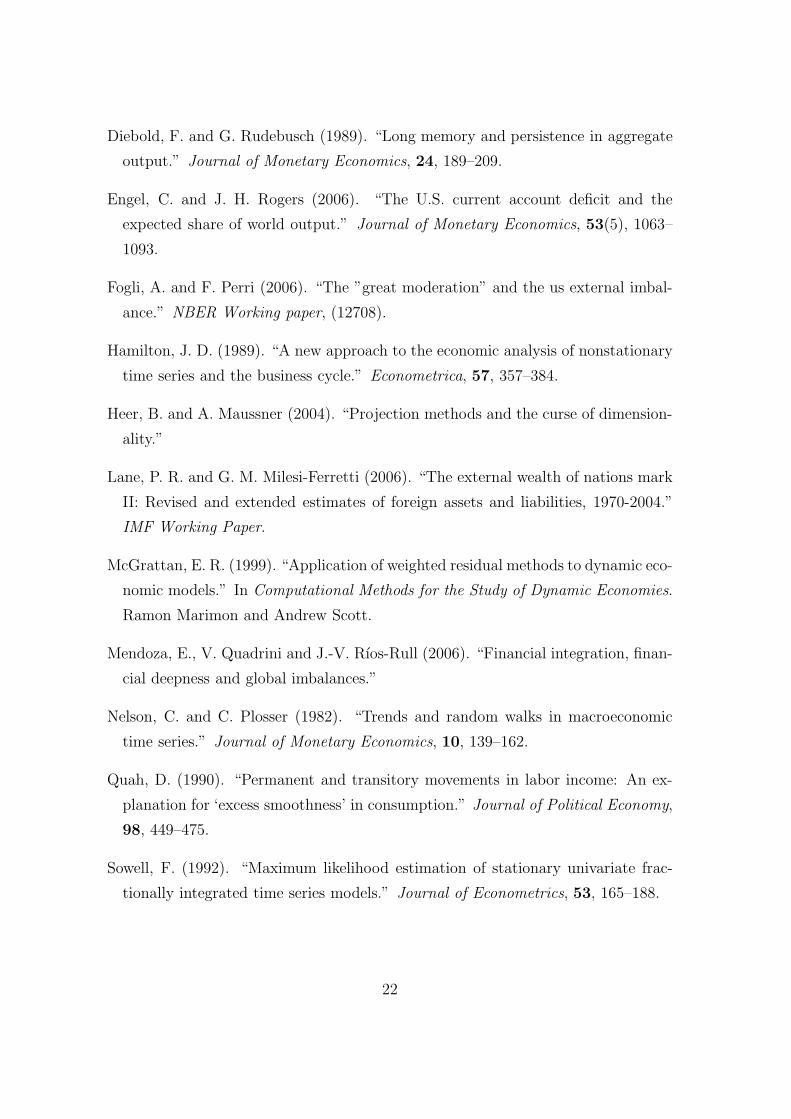
True, external balances have increased over the last ten years. Figure 1 shows
that the cross-sectional dispersion of both net exports and current account balances
4

to GDP ratios has increased since the 1960’s. However, as stressed in Backus, Hen-
riksen, Lambert and Telmer (2005), these balances are not unprecedented. Looking
at historical series for a small sample of countries (Australia, Canada, France, Japan,
Norway, the United Kingdom and the United States), we found that current account
deficits or surpluses over 5% of GDP occurred more than 15% of the time (based
on available observations prior to 1960), with balances above 10% of GDP in nearly
15% of the cases.
2.2 Current account balances are persistent
Current account imbalances are not a temporary feature either. Australia for in-
stance has been running a current account deficit since 1861 except for 29 years.
More than 25% of the time (39 years out of 144), the deficit was greater than 5%
of the Australian GDP, and on average over the last 30 years, it amounted to 4.2%
GDP. Canada has also been running a deficit for most of the 20th century, even if
the situation has reversed over the past few years.
Figure 2 provides some evidence of the persistence of both net exports and cur-
rent account imbalances. The correlations coefficients for current account balances
are slightly higher than for net exports. The main reason is that income flows tend
to increase the persistence of current accounts. Other things being equal, countries
running large trade deficits (surpluses) for several years will accumulate debt (as-
sets) that will generate income flows in the subsequent periods even after the trade
balance has reverted back to zero.
The persistence of current account balances is best seen in the frequency domain.
Figure 3 plots the autocorrelation function (ACF), the periodogram and the spec-
trum of the ratio of quarterly current account balances to GDP for the G7 countries.
All series are seasonally adjusted except for Germany and Italy, which in the case
of Italy explains the peak observed around frequency number 32 corresponding to
a period of one year in the periodogram. See Appendix B for a description of the
way these functions are computed.
For each country, the first graph represents the sample autocorrelation function
(or correlogram) of current account over GDP at all lags between 1 and 50, along
with the 95% confidence interval (the band between the two horizontal lines at
±2/√n, n being the number of observations for each country). The slow decay
5

pattern suggests a very persistent autoregressive process, as sample autocorrelations
appear significantly different from zero even for high lags. In fact, for many series,
we cannot reject the hypothesis of unit root using augmented Dickey-Fuller tests.
The picture for the autocorrelation function is consistent with the two other
graphs. These plot the raw periodogram and its smoothed counterpart, or spectrum
estimate, for frequencies between 1/n and 1/2 (the frequencies are expressed in
cycles per quarter). Both functions provide a decomposition of the variance of the
series by frequency. While there appear to be some short-run (high frequency)
variation, the graphs are clearly dominated by low frequency components, which
can be interpreted as evidence of high persistence.
Figure 4 presents similar graphs for net exports over GDP (seasonally adjusted).
The picture is essentially the same as for current account balances. Income flows
may actually increase the persistence of current account balances compared to net
exports, as income payments depend on accumulated past trade balances.
We have shown that both trade and current account balances can be large and
persistent at the same time. We now examine how these features of the data are
accounted for in a standard international dynamic general equilibrium model.
3 The benchmark model
3.1 A one-good two-country model with complete markets
Our benchmark model is the standard two-country extension of the neoclassical
growth model. The countries are indexed by i = 1, 2. Each country is represented
by one firm, which owns capital and makes investment decisions, and one household.
Time is discrete.
3.1.1 Environment
In each period, an event st drawn from some set S occurs that is observed by
all agents in the economy. The history of events up to period t is denoted by
st = [s0, s1, ..., st]. The unconditional probability of a particular history of events st
is given by π(st).
6

The production function in the two countries is of the Cobb-Douglas form
yi,t(st) = ezi,t(st)ki,t(s
t−1)αni,t(st−1)1−α, (1)
where zi,t(st) is a country-specific technology shock. For simplicity, we assume that
labor supply ni,t is fixed and equal to one in each country.
Capital is assumed to be internationally mobile and accumulates according to
ki,t+1(st) = (1 − δ)ki,t(s
t−1) + xi,t(st), (2)
where xi,t(st) denotes gross investment.
Preferences have the standard additive expected utility structure
Ui(ci) =∞
∑
t=0
∑
st
βtπ(st)ui
(
ci,t(st)
)
, (3)
where the one-period utility function is the same for the two countries and exhibits
constant relative risk aversion ui(c) = c1−γ/(1 − γ).
With complete markets, the budget constraint of country i in period t is given
by
ci,t(st) + xi,t(s
t) +∑
st+1
q(st+1, st)ai,t+1(st+1, s
t) ≤ yi,t(st) + ai,t(st, s
t−1) (4)
where ai,t+1(st+1, st) denote the number of Arrow securities purchased in period t
at history st that pay one unit of the consumption good in period t+ 1 if state st+1
is realized and q(st+1, st) is the price of such securities, expressed in units of the
consumption good in period t.
The aggregate resource constraint for the world economy is
∑
i=1,2
[
ci,t(st) + xi,t(s
t)]
=∑
i=1,2
yi,t(st). (5)
3.1.2 Equilibrium
Since the utility functions are concave, we can solve the social planner’s problem for
the equilibrium allocation. The Pareto problem (with equal Pareto weights on the
two countries) can be written as:
Choose {c1,t(st), c2,t(s
t), x1,t(st), x2,t(s
t)}∞t=0 to maximize
∞∑
t=0
∑
st
βtπ(st)
[
c1,t(st)1−γ
1 − γ+c2,t(s
t)1−γ
1 − γ
]
7

subject to the aggregate budget constraint (5) and the laws of motion for capital
stocks in the two countries (2) for all t, for all st.
The first-order conditions yield the well-known results for a complete markets
economy with full risk-sharing:
• Consumption is the same in the two countries:
c1,t(st) = c2,t(s
t) =1
2
∑
i=1,2
[
yi,t(st) − xi,t(s
t)]
≡ ct(st) (6)
• Capital flows across countries to equalize expected returns on capital:
βEt
{
(
ct+1(st+1)
ct(st)
)−γ(
αezi,t+1(st+1)ki,t+1(st)α−1 + 1 − δ
)
}
= 1, i = 1, 2 (7)
3.1.3 Net exports and current account
Net exports are defined as
nxi,t(st) = yi,t(s
t) − xi,t(st) − ci,t(s
t). (8)
The current account is the sum of net exports, net income flows and current trans-
fers. This definition is consistent with the one used to compute balance of payments
statistics (or national accounts) and does not include changes in asset prices or “valu-
ation effects”, which may be recorded in international investment position statistics.
Under complete markets, current account so defined is always equal to zero, as in-
surance flows (recorded as current transfers) completely offset net exports. Hence
we focus on net exports, the only meaningful aggregate in this set-up.
Besides “technical” considerations, there is another reason that justifies our focus
on net exports. As we have seen in the previous section, the persistence as well as
the magnitude of current account balances are closely linked to those of net exports.
Then accounting for the latter is a necessary step toward explaining the former.
3.1.4 Calibration
We follow Backus et al. (1992) for the calibration of the model’s parameters. In
particular, the technology shocks are modelled as a bivariate autoregression
zt = Λzt−1 + εt (9)
8
where zt = [z1,t, z2,t]′ and εt = [ε1,t, ε2,t]
′ ∼ N(0,Σ).
The elements of Λ and Σ are estimated by running a VAR of order one on
detrended estimates of Solow residuals for the United States and an aggregate of
European countries. They imply persistent technology shocks (the diagonal elements
of Λ are above 0.9) that are also positively correlated across countries. This calibra-
tion also allows for technology spillovers across countries. All parameter values are
summarized in Table 3.
Since the specification of the productivity process ensures that the model is
stationary, we can use a perturbation method to solve the social planner’s problem,
e.g. first or second-order approximation of the first-order conditions or quadratic
approximation of the social planner’s objective function around the steady-state.
This is the standard way to proceed in the real business cycle literature. However the
approximate optimal decision rules so obtained become less accurate as the economy
moves far away from its steady-state. Therefore, we use a weighted residual method
(McGrattan, 1999) and approximate the decision rules with Chebyshev polynomials
using collocation. Though less accurate than the Galerkin method for this type of
models according to Heer and Maussner (2004), the collocation procedure runs much
faster, especially as the dimension of the state-space increases. We use a modified
Newton-Raphson algorithm to solve for the vector of Chebyshev coefficients. The
expectation on the left-hand side of the Euler equation (7) which we use as our
residual function is computed with Gauss-Hermite quadrature.
3.1.5 Results
Following Watson (1993), we assess the performance of the model using spectral
methods. To do so, we generate 1000 simulations of the one-good economy, each
of 195 periods, and compute the average periodogram and spectrum of net exports
over GDP. We then compare the implied spectrum to the ones we computed from
the data for G7 countries. The left panel of Figure 5 plots the average spectrum
from simulated data (plain line) and the spectrum from US data (dotted line) as an
illustration.
From this comparison, it is obvious that the model fails to capture the low
frequency movements observed in the data. The flatness of the artificial spectrum
contrasts with the peak at very low frequencies observed in the data.
9

Figure 6 plots the impulse response function of output, investment, consumption
and net exports to a technology shock in one country. Right after the shock (in the
same period), investment increases sharply in country 1, while it decreases in country
2 as capital flows from one country to the other to equalize expected marginal
returns. The technology shock triggers an increase in output in country 1 which
persists one period after the shock as capital has accumulated. Consumption rises
in both countries. However the increase in consumption in country 1 is smaller than
that of output, so that the trade deficit is mainly driven by changes in investment.
The trade balance reverts to a surplus in the following period as investment drops,
and quickly returns to zero. Hence the absence of persistent imbalances in the
model.
Trade imbalances are also quite large in this frictionless environment. The av-
erage net exports to GDP ratio in absolute value is 5.5% against 2.7% in the data
for OECD countries and this result traditionally motivates the introduction of some
kind of friction in the model. We therefore turn to common modifications of the
model and investigate their effect on the persistence of net exports.
3.2 Adjustment costs
Introducing adjustment costs is standard in the literature and motivated by the need
for some type of friction to dampen the volatility of investment (and therefore net
exports) in response to technology shocks (see Backus et al. (1992) and Baxter and
Crucini (1993)). If adjustment costs help reducing investment fluctuations, which
were shown in the previous section to drive net exports, then one might expect that
adjustment costs also play a role in the persistence of net exports by smoothing
capital flows over time.
We model adjustment costs in the following way:
ψ(ki,t+1(st), ki,t(s
t−1)) = ϕ(ki,t+1(s
t) − ki,t(st−1))2
ki,t(st−1)(10)
Thus only net adjustments to the capital stock are costly. Note that this specification
ensures that production net of investment and adjustment costs is CRS.
We tried different values for the parameter ϕ ranging from 0.1% to 2%, without
any observable effect on the spectrum for net exports over GDP. Larger adjustment
costs limit international capital flows without increasing their persistence.
10

3.3 Incomplete markets
Although the recent years have witnessed a huge development of international finan-
cial markets with the diffusion of new financial products, thereby providing more
empirical support to the complete markets assumption, there remain some obstacles
to international asset trade. If due to these frictions country-specific shocks cannot
be fully insured, countries have a motive for precautionary saving. Faced with a
good shock, countries accumulate foreign assets in provision of less favorable times.
Hence the idea that current account imbalances should be more persistent in models
with incomplete markets or limited commitment.
To test this hypothesis, we consider the most parsimonious form of market incom-
pleteness by restricting the asset structure to a one-period risk-free bond. Country
i’s budget constraint becomes
ci,t(st) + xi,t(s
t) +bi,t+1(s
t)
Rt,t+1(st)≤ yi,t(s
t) + bi,t(st−1), (11)
where bi,t+1(st) denotes the number of risk-free bonds bought by country i in period
t that pay one unit of consumption for sure next period and Rt,t+1(st) is the gross
interest rate between periods t and t+ 1, known in period t (so that 1/Rt,t+1(st) is
the price of a bond in period t).
While as expected bond holdings are very persistent, the spectrum for net exports
over GDP remains flat (see Figure 7). Intuition for this result is given by Baxter
and Crucini (1995). As mentioned earlier the technology process specified by Backus
et al. (1992) allows for spillovers across countries, so that technology shocks spread
across countries over time. In fine most fluctuations in productivity are common
across countries. Then what really matters in terms of insurance and consumption
smoothing is the ability of individuals to smooth consumption across time rather
than across different states, which is precisely what the risk-free bond can be used
for. It is thus not surprising that as regards international capital flows and net
exports the bond economy looks similar to the complete markets one.
We did not impose any borrowing constraints (except for transversality condi-
tions) when solving the model. However considering the results of the simulations
from that model, it seems only a tight constraint would be sometimes binding. The
levels of net liabilities reached by several countries in 2004 (Hungary -97%, New
Zealand -92%, Portugal -70%) do not support such an assumption.
11

One way to have incomplete markets matter may be to introduce preference
shocks, as in Stockman and Tesar (1995). What we have in mind is the case of a
country which is spending a lot, e.g. to host the Olympic Games, thereby building
up external debt that it has to pay back for many periods afterwards. While this may
generate current account persistence thanks to persistent income flows, it is hard to
reconcile with other facts that we also looked at like the persistent differences in per
capita GDP across countries. Moreover it is not clear that this would generate any
persistence in net exports.
3.4 Random walk technology process
The case where technology shocks follow a random walk without spillovers but cor-
related innovations leads to similar results. As shown by Baxter and Crucini (1995),
this alternative specification cannot be rejected from the data on detrended resid-
uals, while it has widely different implications for the international transmission of
business cycles depending on the assumed asset structure. However our results show
that it does not matter for the persistence of the current account. The reason is
that the random walk specification implies a lot of short-run volatility in the cross-
country productivity differences while it does not impose any kind of restriction on
the long-run behavior of productivity in the two countries, e.g. it does not require
long-run convergence of productivity levels, thereby ignoring low frequency features
on the data. These features are the focus of the next section.
4 Long run differences in technology growth
4.1 Evidence
As emphasized by several statistical agencies, there are differences in long-run aver-
age growth rates among advanced countries, both in time-series and in cross-section.
Bassanini and Scarpetta report in an OECD study that a few countries have ex-
perienced an acceleration in per capita GDP growth while other major economies
were lagging behind. The Economic Report to the President 2007 contains similar
observations. Over the past 10 years, per capita GDP and its components like labor
productivity have grown faster in the United States than in most other advanced
12

industrialized country. Further, the report notes that productivity growth acceler-
ated in the United States while it was slowing down in other major industrialized
countries between 2000 and 2005.
Table 4 displays 10-year average productivity growth rates for G7 countries since
1960. These figures confirm that productivity in the United States, as measured by
the Solow residuals, has been growing much faster on average than in all other
G7 countries since 1990. This persistence of productivity growth differences is also
reflected in the spectrum of total factor productivity differences between the US and
an aggregate of ten OECD countries1 (see Figure 8).
While we acknowledge that our measure of total factor productivity may be
inaccurate (see Appendix A for details on the sources and the method used to
compute the Solow residuals), the overall picture is consistent with that obtained
by looking at per capita GDP growth rates, as illustrated by Table 5 and Figure 8.
These findings motivate us to investigate whether our benchmark model with
a more carefully calibrated technology process could account for the persistence of
international capital flows as well as the persistence of cross-country GDP growth
rates.
4.2 Estimating the persistence of technology differences
Motivated by these figures we tried to estimate a process which allowed for persis-
tent differences in technological growth across countries and at the same time was
consistent with economic theory of long-run growth.
In the 1980s a number of studies sought to characterize the nature of the long-run
trend in GDP. Nelson and Plosser (1982), following the work and ideas of Box and
Jenkins (1970), showed that many macroeconomic series could be specified in terms
of unit roots. A discussion about whether macroeconomic time series are better
characterized as integrated or as stationary about a trend followed this contribution
(e.g. Campbell and Mankiw, 1987; Cochrane, 1988).
If technology spreads across countries and the economies have the same structural
parameters, long-run absolute convergence is a prediction of the neoclassical growth
model which we are using in this paper. This prediction has received some empirical
1In addition to the non-U.S. G7 countries, the aggregate includes all OECD countries for which
data were available: Australia, Finland, New Zealand and Norway.
13

supports for OECD countries (Barro and Sala-i Martin, 1992). We will therefore
restrict ourselves to processes which exhibit long-run absolute convergence, hence
rule out non-stationary processes.
Several contributions, like Diebold and Rudebusch (1989) and Sowell (1992),
showed how macroeconomic series while stationary could still exhibit long memory.
We say that xt is fractionally integrated of order d or I(d) if
(1 − L)dxt = ut t = 1, 2, . . .
where L is the lag operator (Lxt = xt−1), d can be any real number greater than
-1 and ut is zero-mean white noise. If d is not an integer, the process is said to be
fractionally integrated. If −0.5 < d < 0.5, xt is said to have long memory, indicating
a non-negligible correlation between observations widely separated in time. The
process is stationary even if d 6= 0. d ∈ [0.5, 1) however implies that the series is
non-stationary but still mean reverting.
Using data on t.f.p. differences among OECD countries between 1970 and 2000,
we estimate d to be around 0.9 when we consider productivity differences between
the United States and the other G7 countries and slightly above 1 in the case of
productivity differences between the United States and an aggregate of OECD coun-
tries. In both cases, a lot of uncertainty surrounds the estimates as the series are
both very short and potentially plagued by measurement errors. In any case, these
estimates stand in contradiction with the theory on long-run convergence of per
capita GDP levels across countries.
4.3 Model specification
Following Aguiar and Gopinath (2007), we rewrite the production function as:
yi,t = ezi,tkαi,t(Gi,tni,t)
1−α, i = 1, 2 (12)
where zi,t is a transitory shock following a stationary autoregressive process and Gi,t
denotes the cumulative product of labor-augmenting “growth” shocks. In particular,
Gi,t = egi,tGi,t−1, i = 1, 2 (13)
where gi,t is a growth shock generated by some autoregressive process to be specified.
14

Alternative modelling approaches include models allowing for both permanent
and transitory innovations in each period (e.g. Quah (1990)) or a regime-switching
model in the tradition started by Hamilton (1989). However, we believe that the
above specification is both very intuitive and easy to deal with whereas it captures
the essential features of data.
While Aguiar and Gopinath (2007) used this specification in the framework of
a small-open economy model, we are looking at a two-country model. Then we
also need to specify the relationship between the technology processes in the two
countries.
We assume that ln(G1,t) and ln(G2,t) are cointegrated with cointegrating vector
[1,−1].2 Let ut ≡ ln(G2,t) − ln(G1,t).
ut = τµt + ρuut−1 + εut (14)
where µt is a random variable drawn from a standard normal distribution whose
value changes with probability λ > 0 every period, and εut is the innovation to the
technology trend difference (εut ∼ N(0, σu)). Different values of the variable µ can be
interpreted as corresponding to different technology epochs, in which one country
is growing faster than the other. This specification thus captures the idea that
countries can diverge, rather than converge, for some periods of time, while keeping
the overall process consistent with absolute convergence in the very long run, as the
unconditional mean of ut is zero.
Given the assumed cointegration relationship, we can solve the model by nor-
malizing all variables in the model by the common technology trend G1,t−1 to ensure
stationarity. For any variable x, let x denote its detrended counterpart:
xt ≡xt
G1,t−1. (15)
This normalization is inocuous for our purpose. What indeed matters for net exports
or current account is the difference in technology ln(G2,t)− ln(G1,t). In steady-state
where G = 1 in both countries, there is no current account imbalance.
2A regression of the Solow residuals in the US on the residuals in an aggregate of ten OECD
countries yields a coefficient that is not significantly different from one, so we find some support
for that assumption in the data.
15

With normalized variables, the Euler equations used to solve the model become
(we dropped the history-dependent notation):
βe−γg1,tEt
{
(
ct+1
ct
)−γ(
αe(z1,t+1+(1−α)g1,t+1)kα−11,t+1 + 1 − δ
)
}
= 1 (16)
βe−γg1,tEt
{
(
ct+1
ct
)−γ(
αe(z2,t+1+(1−α)g2,t+1)e(1−α)ut kα−12,t+1 + 1 − δ
)
}
= 1 (17)
where ut is defined by Equation (14).
4.4 Calibration
The difference in the logarithms of technology levels l between the two country is
given by:
tfp2,t − tfp1,t = z2,t − z1,t + (1 − α)ut (18)
The question is how to pin down the process for ut and for zi,t, i = 1, 2. Let
zi,t = ρzzi,t−1 + εzi,t. If for simplicity we fix the technology level in country 1 to one,
ez1,tG1−α1,t = 1 for all t and let g2,t = ut − ut−1, then we still need to get calibrated
values for six parameters: ρz (autoregressive coefficient of the transitory shock), σz
(standard deviation of the transitory shocks), ρu (autoregressive coefficient of the
growth shock), τ (standard deviation of the technological shifts), λ (probability of a
technological shift) and σu (standard deviation of the innovations to the technology
trend differences).
We may impose ρz = ρu ≡ ρ and estimate an AR(1), on the differences of Solow
residuals between the US and an OECD aggregate. This yields ρ = 0.97 and a
standard deviation of the residuals equal to 0.007. The problem is now how to split
this standard deviation between the two components: growth shocks and transitory
shocks. Let us set σu = 0 and focus on σz, τ . and λ. We consider four cases,
summarized in Table 6: high and low variance of the transitory shock differences
compared to the variance of the technological changes, and high and low values of λ,
which determines the average frequency of those changes. Other parameter values
were taken from Backus et al. (1992) (see Table 3).
All four parameterizations yield a simulated spectrum for quarterly productivity
differences roughly similar to the one computed from the data for the United States
and our aggregate of OECD countries (dashed lines on Figure 9). This resemblance is
16

due to the fact that very short series (195 periods for the simulated series, 123 periods
for measured productivity differences in the data) were used to compute the spectra
and illustrates the difficulty of identifying the “true” technology specification directly
from the data on Solow residuals, even without thinking about measurement issues
in the computation of these residuals. While the four parameterizations cannot be
rejected from the data, they yield very different results in terms of persistence of
net exports over GDP.
4.5 Results
Figure 10 plots the average ACF and spectrum of the ratio of net exports over
GDP from a large number of simulations of 195 periods of the model for the four
parameterizations of the technology process. The graphs show striking differences.
While persistence is low for parameterizations 1 and 3, when the variance of the
transitory shock differences is set equal to the variance of the technological changes,
it is much higher when we increase the variance of the technological changes. Thus
for some parameterization, the model is successful at capturing the low frequency
dimension of the data. The key parameter is the relative variance of the two types
of shocks, rather than the frequency of technological shifts.
For all parameterizations, the average net exports to GDP ratio (in absolute
values) lies between 5.3% and 6.0%. While this is higher than what is observed in
OECD countries (2.7%), the difference may be accounted for by the absence of any
form of adjustment costs in this version of the model. As explained in section 3.2,
the usual reason for introducing adjustment costs in this type of models is precisely
to dampen the volatility of investment, which reduces the size of net exports.
The spectrum of per capita GDP differences generated from the model is similar
across parameterizations and very close to what is observed in the data (Figure 11).
Again this does not allow us to reject any of the parameterizations.
Crucial for the success of the model is the persistence of growth differences im-
plied by our specification of the technology process. Detrending the Solow residuals
using the Hodrick-Prescott filter or other kind of band-pass or high-pass filter, as is
done in Backus et al. (1992) and other international business cycle studies, removes
most low frequency movements in technology. Part of the reason why the various
extensions of the benchmark model failed to reproduce the low frequency dynamics
17

in net exports is because these extensions do not provide sufficiently strong propaga-
tion mechanisms for high-frequency shocks. In a one-country set-up, a similar point
was emphasized by Cogley and Nason (1995). Our results show that a more careful
specification of the technology process which captures the observed long-run growth
differences across countries is both necessary and sufficient to get the spectrum of
the trade balance right.
5 Conclusion
Three things should be taken away from this paper. First, the paper stresses the
importance of the low frequency features of the data on net exports and current
accounts that have been neglected by the recent international business cycle lit-
erature. Thereby we stick to the sometimes overlooked original objective of real
business cycles models to provide a consistent framework to account for both long-
run movements and business cycle fluctuations. Second, we show that deviations
from the frictionless, complete-markets environment are not sufficient to account
for the persistence of external imbalances and that carefully specifying a technology
process consistent with the low frequency features of the data on productivity and
per capita GDP is required to obtain such a result. We argue that long-run shifts
in technology more than transitory shocks are what matter for current account dy-
namics, and show that once these shifts are taken into account, current account
imbalances can be both large and very persistent, as is the case in the United States
today. In fact, and this is our third main result, given the observed persistence of
productivity and per capita GDP differences, net exports over GDP in the model
are substantially larger than what is observed.
We leave many questions open. In particular, we did not address the origins
of these long-run productivity growth differences. In our model with fixed labor
supply, technology is a convenient concept that can be interpreted in various ways
and its process may capture both “pure” technological changes as well as changes
in labor supply for instance. Trying to endogenize technology has been the subject
of a lot of research. Looking at this issue from an international perspective might
provide new insights.
18

Appendix A : Data sources
Current account, net exports and GDP data after 1960 were obtained from Datas-
tream (national sources) and the OECD Quarterly National Accounts Database.
Historical series are from Backus et al. (2005).
The expression used to compute Solow residuals in country i at time t is derived
from the production function (1) in log:
zi,t = log yi,t − α log ki,t − (1 − α) logni,t, (A-1)
where for notational concision we dropped the history-dependent notation. ni,t is
computed as the product of total employment and the average number of hours
worked per employee in the business sector (the average number of hours worked for
all sectors is generally not available). ki,t is approximated by the capital stock of the
business sector, excluding house building, in real terms. yi,t is real GDP. To allow
international comparisons of productivity levels, both capital stocks and GDP were
converted into US dollars. We use country-specific labor shares (1−α) computed by
Bernanke and Gurkaynak (2001). Except for labor shares data, all series come from
the OECD Main Economic Indicators, Economic Outlook or Quarterly National
Accounts databases.
Appendix B : Tools for the spectral analysis of time
series
Consider the covariance-stationary series {xt}n−1t=0 with mean x. The sample autocor-
relation at lag r is defined as the ratio of the autocovariance at lag r to the variance
of the series:
ˆacf r =crc0
(B-1)
where cr = 1n
∑n−1t=|r|(xt− x)(xt−|r|− x). This definition which corresponds to a biased
estimator of the autocovariance ensures that the sample autocorrelation lies between
-1 and 1. The periodogram is the Fourier transform of the sample autocovariance
sequence:
I(ωj) =1
2π
∑
|r|<n
cre−irωj (B-2)
19

where ωj = 2πj/n is the jth Fourier frequency. The periodogram integrates to the
sample variance:∫ π
−π
I(ω)dω = c0 (B-3)
It follows that the ordinate I(ωj) has a nice interpretation as the portion of the
sample variance due to the harmonic component at frequency ωj . Note that it can
be rewritten as:
I(ωj) =1
2π
[
c0 + 2
n−1∑
r=1
cr(eirωj + e−irωj)
]
=1
2π
[
c0 + 2
n−1∑
r=1
cr cos(ωjr)
]
(B-4)
The spectrum is obtained by smoothing the periodogram using a q-period Bartlett
window, where the choice of the bandwith parameter q results from a trade-off
between reducing the variance and minimizing the bias of the estimate. Then,
f(ωj) =1
2π
∑
|r|<q
(1 − |r|/q)cre−irωj
=1
2π
[
c0 + 2
q−1∑
r=1
(1 − |r|/q)cr cos(ωjr)
]
(B-5)
20

References
Aguiar, M. and G. Gopinath (2007). “Emerging market business cycles: The cycle
is the trend.” Journal of Political Economy, 115(1), 69–102.
Backus, D., E. Henriksen, F. Lambert and C. Telmer (2005). “Current account fact
and fiction.”
Backus, D. K., P. J. Kehoe and F. E. Kydland (1992). “International real business
cycles.” Journal of Political Economy, 100(4), 745–775.
Barro, R. J. and X. Sala-i Martin (1992). “Convergence.” Journal of Political
Economy, 100(2), 223–251.
Bassanini, A. and S. Scarpetta (2002). “The driving forces of economic growth:
Panel data evidence for the OECD countries.” OECD Economic Studies, 33.
Baxter, M. and M. J. Crucini (1993). “Explaining saving-investment correlations.”
American Economic Review, 83(3), 416–436.
Baxter, M. and M. J. Crucini (1995). “Business cycles and the asset structure of
foreign trade.” International Economic Review, 36(4), 821–854.
Bernanke, B. S. and R. S. Gurkaynak (2001). “Is growth exogenous? Taking
Mankiw, Romer and Weil seriously.” NBER Working Paper, (8365).
Box, G. and G. Jenkins (1970). Time Series Analysis, Forecasting and Control.
Holden Day, San Francisco.
Caballero, R. J., E. Farhi and P.-O. Gourinchas (2006). “An equilibrium model of
“global imbalances” and low interest rates.”
Campbell, J. Y. and N. G. Mankiw (1987). “Are output fluctuations transitory?”
The Quarterly Journal of Economics, 102(4), 857–80.
Cochrane, J. (1988). “How big is random walk in GDP?” Journal of Political
Economy, 96(5), 893–92.
Cogley, T. and J. M. Nason (1995). “Output dynamics in real-business-cycle mod-
els.” American Economic Review, 85(3), 492–511.
21
Diebold, F. and G. Rudebusch (1989). “Long memory and persistence in aggregate
output.” Journal of Monetary Economics, 24, 189–209.
Engel, C. and J. H. Rogers (2006). “The U.S. current account deficit and the
expected share of world output.” Journal of Monetary Economics, 53(5), 1063–
1093.
Fogli, A. and F. Perri (2006). “The ”great moderation” and the us external imbal-
ance.” NBER Working paper, (12708).
Hamilton, J. D. (1989). “A new approach to the economic analysis of nonstationary
time series and the business cycle.” Econometrica, 57, 357–384.
Heer, B. and A. Maussner (2004). “Projection methods and the curse of dimension-
ality.”
Lane, P. R. and G. M. Milesi-Ferretti (2006). “The external wealth of nations mark
II: Revised and extended estimates of foreign assets and liabilities, 1970-2004.”
IMF Working Paper.
McGrattan, E. R. (1999). “Application of weighted residual methods to dynamic eco-
nomic models.” In Computational Methods for the Study of Dynamic Economies.
Ramon Marimon and Andrew Scott.
Mendoza, E., V. Quadrini and J.-V. Rıos-Rull (2006). “Financial integration, finan-
cial deepness and global imbalances.”
Nelson, C. and C. Plosser (1982). “Trends and random walks in macroeconomic
time series.” Journal of Monetary Economics, 10, 139–162.
Quah, D. (1990). “Permanent and transitory movements in labor income: An ex-
planation for ‘excess smoothness’ in consumption.” Journal of Political Economy,
98, 449–475.
Sowell, F. (1992). “Maximum likelihood estimation of stationary univariate frac-
tionally integrated time series models.” Journal of Econometrics, 53, 165–188.
22

Stockman, A. C. and L. L. Tesar (1995). “Tastes and technology in a two-country
model of the business cycle: Explaining international comovements.” American
Economic Review, 85(1), 168–185.
Watson, M. W. (1993). “Measures of fit for calibrated models.” Journal of Political
Economy, 101(6), 1011–1041.
23

Table 1: Trade and current account balances in OECD countries
Trade balances in % of GDP (2005)
Largest deficits Largest surplusses
Iceland -12.4% Luxembourg 21.3%
Portugal -8.9% Norway 17.2%
Greece -7.2% Ireland 12.7%
Turkey -6.6% Sweden 7.7%
United States -5.8% Netherlands 7.7%
Spain -5.4% Switzerland 6.8%
Slovakia -5.1% Finland 5.6%
United Kingdom -3.7% Germany 5.2%
Current account balances in % of GDP (2005)
Largest deficits Largest surplusses
Iceland -16.5% Norway 15.5%
Portugal -9.2% Switzerland 15.3%
New Zealand -9.0% Luxembourg 11.8%
Slovakia -8.6% Netherlands 7.7%
Spain -7.4% Sweden 7.1%
Hungary -6.8% Finland 4.9%
Turkey -6.4% Germany 4.0%
United States -6.4% Japan 3.7%
Sources: Datastream/National sources.
24

Table 2: Summary statistics (based on quarterly data)
Mean Autocorrelation at lag:
Variable (of absolute values) 4 8 12 20
net exports/GDP 2.7% 0.76 0.64 0.55 0.47
current account/GDP 3.1% 0.77 0.68 0.58 0.53
Sources: Datastream/National sources and OECD.
Computations based on data for 18 OECD countries. The sample period covers
1957:01-2005:03.
Table 3: Benchmark parameter values
Preferences β = .99, γ = 2
Technology α = .36, δ = .025
Productivity process Λ =
[
.906 .088
.088 .906
]
Σ = .008522 ×[
1 0.258
0.258 1
]
Table 4: Average annual t.f.p. growth rates across G7 countries (in %)
1970-80 1980-90 1990-00 2000-05
United States 0.76 0.78 1.49 1.36
Canada 0.74 0.50 1.11 0.91
United Kingdom - 1.03 1.37 1.02
France - 1.22 0.78 0.90
Germany 2.11 1.09 1.13 0.86
Italy 3.86 1.35 0.93 -0.56
Japan - 1.38 0.42 1.44
Source: OECD, authors’ calculations.
25

Table 5: Average annual per capita GDP growth rates across G7 countries (in %)
1960-701 1970-80 1980-90 1990-00 2000-04
United States 2.89 2.21 2.11 1.98 1.43
Canada 3.32 2.60 1.69 1.53 1.80
United Kingdom 2.24 2.25 2.16 1.99 2.25
France 3.42 2.97 1.70 1.47 1.33
Germany 3.49 2.82 1.72 0.85 0.73
Italy 4.62 5.16 2.16 1.37 0.87
Japan 9.07 3.50 3.23 1.00 1.24
1France: 1963-1970. Source: OECD.
Table 6: Different parametrization of the technology process
Parametrization 1 σz = τ = 0.006, λ = 1/20 (on average technological changes
happen every 5 years)
Parametrization 2 σz = 0.5τ = 0.0043, λ = 1/20
Parametrization 3 σz = τ = 0.006, λ = 1/40 (on average technological changes
happen every 10 years)
Parametrization 4 σz = 0.5τ = 0.0043, λ = 1/40
26
Figure 1: External deficits since 1960
−.1
0.1
.2R
atio
of N
et E
xpor
ts to
GD
P
1960 1970 1980 1990 2000 2010Year
−.1
0.1
.2R
atio
of C
urre
nt A
ccou
nt to
GD
P
1960 1970 1980 1990 2000 2010Year
The data cover 18 OECD countries: Australia, Austria, Canada, Denmark, Finland,France, Germany, Italy, Japan, Netherlands, New Zealand, Norway, Portugal, Spain, Swe-den, Switzerland, United Kingdom and the United States.
27

Figure 2: Persistence of net exports and current accounts
−.2
−.1
0.1
.24
Qua
rter
s A
head
−.2 −.1 0 .1 .2Ratio of Net Exports to GDP
−.2
−.1
0.1
.28
Qua
rter
s A
head
−.2 −.1 0 .1 .2Ratio of Net Exports to GDP
−.2
−.1
0.1
.212
Qua
rter
s A
head
−.2 −.1 0 .1 .2Ratio of Net Exports to GDP
−.2
−.1
0.1
.220
Qua
rter
s A
head
−.2 −.1 0 .1 .2Ratio of Net Exports to GDP
−.2
−.1
0.1
.24
Qua
rter
s A
head
−.2 −.1 0 .1 .2Ratio of Current Account to GDP
−.2
−.1
0.1
.28
Qua
rter
s A
head
−.2 −.1 0 .1 .2Ratio of Current Account to GDP
−.2
−.1
0.1
.212
Qua
rter
s A
head
−.2 −.1 0 .1 .2Ratio of Current Account to GDP
−.2
−.1
0.1
.220
Qua
rter
s A
head
−.2 −.1 0 .1 .2Ratio of Current Account to GDP
Quarterly data for 18 OECD countries: Australia, Austria, Canada, Denmark, Finland,France, Germany, Italy, Japan, Netherlands, New Zealand, Norway, Portugal, Spain, Swe-den, Switzerland, United Kingdom and the United States.
28

Figure 3: Current account balance/GDP
0 10 20 30 40 50
−1
−0.5
0
0.5
1
ACF: Canada, n=195
0 0.1 0.2 0.3 0.4 0.50
1
2
3
4
5
6Periodogram: Canada
0 0.1 0.2 0.3 0.4 0.50
0.5
1
1.5Spectrum: Canada
0 10 20 30 40 50
−1
−0.5
0
0.5
1
ACF: France, n=75
0 0.1 0.2 0.3 0.4 0.50
1
2
3
4
5Periodogram: France
0 0.1 0.2 0.3 0.4 0.50
0.5
1
1.5Spectrum: France
0 10 20 30 40 50
−1
−0.5
0
0.5
1
ACF: Germany, n=59
0 0.1 0.2 0.3 0.4 0.50
0.5
1
1.5
2Periodogram: Germany
0 0.1 0.2 0.3 0.4 0.50
0.2
0.4
0.6
0.8
1Spectrum: Germany
0 10 20 30 40 50
−1
−0.5
0
0.5
1
ACF: Italy, n=131
0 0.1 0.2 0.3 0.4 0.50
0.5
1
1.5
2
2.5Periodogram: Italy
0 0.1 0.2 0.3 0.4 0.50
0.1
0.2
0.3
0.4
0.5
0.6
0.7
0.8Spectrum: Italy
0 10 20 30 40 50
−1
−0.5
0
0.5
1
ACF: Japan, n=82
0 0.1 0.2 0.3 0.4 0.50
0.5
1
1.5
2
2.5Periodogram: Japan
0 0.1 0.2 0.3 0.4 0.50
0.2
0.4
0.6
0.8
1Spectrum: Japan
0 10 20 30 40 50
−1
−0.5
0
0.5
1
ACF: UK, n=195
0 0.1 0.2 0.3 0.4 0.50
0.5
1
1.5
2
2.5
3
3.5
4Periodogram: UK
0 0.1 0.2 0.3 0.4 0.50
0.5
1
1.5Spectrum: UK
0 10 20 30 40 50
−1
−0.5
0
0.5
1
ACF: US, n=183
0 0.1 0.2 0.3 0.4 0.50
1
2
3
4
5
6Periodogram: US
0 0.1 0.2 0.3 0.4 0.50
0.5
1
1.5Spectrum: US
29

Figure 4: Net exports/GDP
0 10 20 30 40 50
−1
−0.5
0
0.5
1
ACF: Canada, n=179
0 0.1 0.2 0.3 0.4 0.50
1
2
3
4
5Periodogram: Canada
0 0.1 0.2 0.3 0.4 0.50
0.5
1
1.5Spectrum: Canada
0 10 20 30 40 50
−1
−0.5
0
0.5
1
ACF: France, n=110
0 0.1 0.2 0.3 0.4 0.50
1
2
3
4
5
6
7
8Periodogram: France
0 0.1 0.2 0.3 0.4 0.50
0.5
1
1.5Spectrum: France
0 10 20 30 40 50
−1
−0.5
0
0.5
1
ACF: Germany, n=59
0 0.1 0.2 0.3 0.4 0.50
0.5
1
1.5
2
2.5Periodogram: Germany
0 0.1 0.2 0.3 0.4 0.50
0.5
1
1.5Spectrum: Germany
0 10 20 30 40 50
−1
−0.5
0
0.5
1
ACF: Italy, n=103
0 0.1 0.2 0.3 0.4 0.50
1
2
3
4
5Periodogram: Italy
0 0.1 0.2 0.3 0.4 0.50
0.5
1
1.5Spectrum: Italy
0 10 20 30 40 50
−1
−0.5
0
0.5
1
ACF: Japan, n=103
0 0.1 0.2 0.3 0.4 0.50
0.5
1
1.5
2Periodogram: Japan
0 0.1 0.2 0.3 0.4 0.50
0.5
1
1.5Spectrum: Japan
0 10 20 30 40 50
−1
−0.5
0
0.5
1
ACF: UK, n=195
0 0.1 0.2 0.3 0.4 0.50
0.5
1
1.5
2
2.5
3
3.5
4Periodogram: UK
0 0.1 0.2 0.3 0.4 0.50
0.5
1
1.5Spectrum: UK
0 10 20 30 40 50
−1
−0.5
0
0.5
1
ACF: US, n=195
0 0.1 0.2 0.3 0.4 0.50
1
2
3
4
5
6Periodogram: US
0 0.1 0.2 0.3 0.4 0.50
0.5
1
1.5Spectrum: US
30

Figure 5: Spectrum of net exports/GDP implied by the benchmark model
0 10 20 30 40 50
−1
−0.8
−0.6
−0.4
−0.2
0
0.2
0.4
0.6
0.8
1
ACF
0 0.1 0.2 0.3 0.4 0.50
0.2
0.4
0.6
0.8
1
1.2
1.4Spectrum
Figure 6: Impulse response functions to a 1% productivity shock in country 1
(benchmark model)
0 10 20 30 40 500
0.002
0.004
0.006
0.008
0.01technology
z1z2
0 10 20 30 40 500.995
1
1.005
1.01
1.015output
y1y2
0 10 20 30 40 50−0.4
−0.2
0
0.2
0.4net investment
ni1ni2
0 10 20 30 40 501
1.002
1.004
1.006
1.008consumption
0 10 20 30 40 50−0.1
−0.05
0
0.05
0.1net exports/GDP
nx1nx2
31

Figure 7: Spectrum of net exports/GDP implied by an incomplete markets model
with Backus et al. (1992) calibration
0 5 10 15 20 25 30 35 40 45 50
−1
−0.8
−0.6
−0.4
−0.2
0
0.2
0.4
0.6
0.8
1
ACF
0 0.05 0.1 0.15 0.2 0.25 0.3 0.35 0.4 0.45 0.50
0.2
0.4
0.6
0.8
1
1.2
1.4Spectrum
Figure 8: Spectrum of productivity and per capita GDP differences US/OECD
aggregate
0 0.1 0.2 0.3 0.4 0.50
0.2
0.4
0.6
0.8
1
1.2
1.4Productivity differences
0 0.1 0.2 0.3 0.4 0.50
0.2
0.4
0.6
0.8
1
1.2
1.4Per capita GDP differences
32

Figure 9: Spectrum of productivity differences for the different parameterizations
0 0.05 0.1 0.15 0.2 0.25 0.3 0.35 0.4 0.45 0.50
0.5
1
1.5Parameterization 1
0 0.05 0.1 0.15 0.2 0.25 0.3 0.35 0.4 0.45 0.50
0.5
1
1.5Parameterization 2
0 0.05 0.1 0.15 0.2 0.25 0.3 0.35 0.4 0.45 0.50
0.5
1
1.5Parameterization 3
0 0.05 0.1 0.15 0.2 0.25 0.3 0.35 0.4 0.45 0.50
0.5
1
1.5Parameterization 4
33

Figure 10: ACF and spectrum of net exports/GDP for the different parameteriza-
tions
Parametrization 1
0 5 10 15 20 25 30 35 40 45 50
−1
−0.8
−0.6
−0.4
−0.2
0
0.2
0.4
0.6
0.8
1
ACF
0 0.05 0.1 0.15 0.2 0.25 0.3 0.35 0.4 0.45 0.50
0.2
0.4
0.6
0.8
1
1.2
1.4Spectrum
Parametrization 2
0 5 10 15 20 25 30 35 40 45 50
−1
−0.8
−0.6
−0.4
−0.2
0
0.2
0.4
0.6
0.8
1
ACF
0 0.05 0.1 0.15 0.2 0.25 0.3 0.35 0.4 0.45 0.50
0.2
0.4
0.6
0.8
1
1.2
1.4Spectrum
Parametrization 3
0 5 10 15 20 25 30 35 40 45 50
−1
−0.8
−0.6
−0.4
−0.2
0
0.2
0.4
0.6
0.8
1
ACF
0 0.05 0.1 0.15 0.2 0.25 0.3 0.35 0.4 0.45 0.50
0.2
0.4
0.6
0.8
1
1.2
1.4Spectrum
Parametrization 4
0 5 10 15 20 25 30 35 40 45 50
−1
−0.8
−0.6
−0.4
−0.2
0
0.2
0.4
0.6
0.8
1
ACF
0 0.05 0.1 0.15 0.2 0.25 0.3 0.35 0.4 0.45 0.50
0.2
0.4
0.6
0.8
1
1.2
1.4Spectrum
34

Figure 11: Spectrum of per capita GDP differences for the different parameteriza-
tions
0 0.05 0.1 0.15 0.2 0.25 0.3 0.35 0.4 0.45 0.50
0.5
1
1.5Parameterization 1
0 0.05 0.1 0.15 0.2 0.25 0.3 0.35 0.4 0.45 0.50
0.5
1
1.5Parameterization 2
0 0.05 0.1 0.15 0.2 0.25 0.3 0.35 0.4 0.45 0.50
0.5
1
1.5Parameterization 3
0 0.05 0.1 0.15 0.2 0.25 0.3 0.35 0.4 0.45 0.50
0.5
1
1.5Parameterization 4
35
Related Documents