Technology management models for marine seismic ... - CORE

Technology management models for

marine seismic acquisition projects

Author

LEI LI

Student‘s Registration Number

214752

Supervisor

Professor Ove T Gudmestad

DEPARTMENT OF CIVIL AND MECHANICAL

ENGINEERING

FACULTY OF SCIENCE AND TECHNOLOGY

UNIVERSITY OF STAVANGER NORWAY

March 2013

brought to you by COREView metadata, citation and similar papers at core.ac.uk

provided by NORA - Norwegian Open Research Archives

https://core.ac.uk/display/30922089?utm_source=pdf&utm_medium=banner&utm_campaign=pdf-decoration-v1

1 / 83

Technology management models for marine

seismic acquisition projects

Author

LEI LI

Student‘s Registration Number

214752

A thesis submitted in partial fulfillment of the requirement for the degree of

M.Sc. Asset Mangement

Thesis Supervisor:

Professor Ove T Gudmestad

DEPARTMENT OF

CIVIL AND MECHANICAL ENGINEERING

FACULTY OF SCIENCE AND TECHNOLOGY

UNIVERSITY OF STAVANGER NORWAY

STAVANGER

February 2013

2 / 83

Acknowledgement

First and foremost, I would like to express my utmost gratitude to my supervisor Professor

Ove Tobias Gudmestad who helped me in developing this master thesis with professional

guidance, suggestions and comments, I will never forget his sincerity and encouragement on

this thesis writing.

I am greatly appreciated to my company COSL and GEO-COSL for giving me the

opportunity to study master degree aboard; my debt to them is beyond measure, because I am

sure I will benefit from this study for rest of my life.

My further sincere thanks go to my colleagues and classmates of COSL who helped me in

learning and living in Stavanger, Norway; I want to especially thank Hu Pengfei, Xu

Fengyang, Peng Guicang, Li Fengyun and my roommates: Wu Zixian, Yu Peigang, and Chen

Wenming.

During master thesis writing, I would like to thank Cao Zhanquan，Li Jianmin, Zhang

Hongxing, Wei Chengwu, Wang Jianguo, Liu Genyuan, Cai Yue, Chen Gang, and Zhang

Lijun for their help, support and encouragement.

Last but not the least; I am grateful to my family, especially my parents and my wife, thank

you so much for the support that you have given me.

Beijing, China

LEI LI

李磊

3 / 83

Abstract

A marine seismic exploration project is a high investment project with complex procedures,

state of art management models should be implemented to solve the limitations and problems

encountered in marine environment projects.

High investments in the seismic exploration need high working efficiency. So the specifics of

technology for marine seismic acquisition should focus on how to improve the efficiency of

marine seismic exploration,

Marine seismic data acquisition vessels are specialized vessels that towing a number of

streamers (cables) and air guns, vessels characteristics and stability are all discussed and

analyzed in this thesis.

Management strategy for equipment procurement and management of the spare parts that

support the projects are crucial to any projects, they are the safeguard to make sure the marine

seismic exploration follows the plan, and effective ways to reduce cost.

An advanced maintenance technology will save lots of money and will be welcomed by all

project managers. Maintenance technologies are also discussed in this thesis to give managers

a clear concept of equipment replacement, optimize their management.

Risk involved in the acquisition project management shall be emphasized by project managers

and executors. Risks methodologies used to analyze risks in marine seismic data acquisitions

should be concerned by all managers, in this thesis, we mainly focus on operational risk and

environment risk.

4 / 83

Abstract in Chinese

海洋地震勘探项目是一个具有复杂程序的高投入的项目，这个特性决定了我们需要将

先进的管理模式应用到项目的实施中，以解决实际操作中遇到的问题。

在地震勘探的高投资需要较高的工作效率，因此，海洋地震数据采集中的关键技术应

将重点放在如何提高海上地震勘探的工作效率中。

海上地震数据采集船是经过专门设计的特种作业船，他在作业过程中会一直拖曳电缆

和空气枪，作业方式决定了勘探船的独有特性，在本篇论文中，我们着重讨论和分析

了勘探船的特性和稳定性。

设备采购和备件管理策略在项目实施中起到了非常关键的作用，这是保障项目顺利实

施的基础，同时又是最立竿见影的减少项目成本的方法。

先进的维修技术将节省大量的金钱，因此会受到项目经理们欢迎。先进的设备维护保

养理念会使管理人员能够更加深层的了解他们的设备，实现更加优化的管理。

项目管理人员应该在项目实施的过程中加强对项目的风险分析，管理人员应该重视项

目风险分析的方法论，这篇论文中着重讨论了操作风险分析和环境风险分析。

5 / 83

Table of Content Abstract .............................................................................................................................................. 3

Chapter 1 Introduction ...................................................................................................................... 12

1.1 Background ......................................................................................................................... 12

1.2 Objective and method ......................................................................................................... 13

1.3 The scope of the work ......................................................................................................... 13

1.4 The structure of the thesis ................................................................................................... 13

Chapter 2 Overview of marine seismic acquisition ............................................................................ 14

2.1 Introduction and underlying principles ................................................................................ 14

2.2 Propagation fundamentals .................................................................................................. 15

2.2.1 P waves theory .......................................................................................................... 15

2.2.2 S waves theory .......................................................................................................... 15

2.3 Towed marine seismic acquisition methods ......................................................................... 16

2.3.1 Towed 2D acquisition ............................................................................................... 16

2.3.2 Towed 3D acquisition ............................................................................................... 17

2.4 Conventional marine seismic equipment ........................................................................ 18

2.4.1 Seismic streamer ....................................................................................................... 18

2.4.2 Seismic sources......................................................................................................... 21

2.5 New developments and advance technologies .................................................................... 22

2.5.1 Streamer technology improvement ............................................................................ 23

2.5.2 De-ghosting technology ............................................................................................ 23

2.5.3 More Azimuth Marine Acquisition ............................................................................ 24

Chapter 3 Marine seismic vessel characteristics................................................................................. 28

3.1 What are marine seismic vessels ......................................................................................... 28

3.2 Vessel characteristics........................................................................................................... 29

3.2.1 General characteristics .............................................................................................. 29

3.2.2 Vessel design ............................................................................................................ 30

6 / 83

3.3 Vessel movements............................................................................................................... 31

3.4 Marine seismic vessel stability consideration ....................................................................... 32

3.5 Vessel operational constraints ............................................................................................. 35

3.5.1 Turning radius constraint .......................................................................................... 36

3.5.2 Vessel speed constraint ............................................................................................. 36

3.5.3 Ambient environment constraint ............................................................................... 36

3.6 Class notation for seismic vessels ........................................................................................ 37

Chapter 4 Acquisition project management ....................................................................................... 38

4.1 Creating a project network .................................................................................................. 38

4.1.1 Sequencing activities................................................................................................. 38

4.1.2 The network diagram ................................................................................................ 39

4.1.3 Creating a network .................................................................................................... 40

4.2 Procurement management .................................................................................................. 41

4.3 Equipment maintenance technology ................................................................................... 44

4.3.1 Preventive maintenance............................................................................................. 44

4.3.2 Predictive Maintenance ............................................................................................. 45

4.4 Maintenance interval calculation models............................................................................. 46

4.4.1 Age replacement model............................................................................................. 46

4.4.2 The Block replacement model ................................................................................... 47

4.4.3 Minimal repair block replacement ............................................................................. 48

4.5 Spare parts management .................................................................................................... 48

4.5.1 What spare parts to store? ......................................................................................... 49

4.5.2 How many spare parts to store? ................................................................................. 50

4.5.3 Where to store the spare parts? .................................................................................. 52

Chapter 5 Risk analysis and management .......................................................................................... 54

5.1 Risk and risk analysis methodology ...................................................................................... 54

7 / 83

5.2 Risk management methodologies ........................................................................................ 56

5.2.1 Hazard identification ................................................................................................. 57

5.2.2 Qualitative analysis ................................................................................................... 58

5.3 Risk involved in marine seismic exploration ......................................................................... 61

5.3.1 Personnel operational risk ......................................................................................... 61

5.3.2 Environmental risk .................................................................................................... 62

5.3.3 Weather risk ............................................................................................................. 64

5.3.4. Supply chain risk ..................................................................................................... 64

Chapter 6 Conclusions and Recommendations .................................................................................. 66

References ........................................................................................................................................ 67

Appendix 1: LCC analysis ................................................................................................................ 71

Appendix 2: DNV Rules for Ships .................................................................................................... 76

8 / 83

List of Figures

Figure 2. 1 Marine seismic acquisition principle (Odland, 2009a) ............................................. 14

Figure 2. 2 P waves simulation (credit: Tech Museum of Innovation 2012)................................ 15

Figure 2. 3 S wave simulation (credit: Tech Museum of Innovation 2012).................................. 16

Figure 2. 4 2D acquisition feather ............................................................................................. 17

Figure 2. 5 3D survey with a ‘racetrack’ pattern (credit: HYSY718, GEO-COSL)...................... 18

Figure 2. 6 Fluid filled streamer (left) and solid streamer (right)

(credit: HYSY718 and HYSY720 GEO-COSL) .................................................................... 19

Figure 2. 7 Devices attached on streamers (credit: ION geophysical) ........................................ 20

Figure 2. 8 Tailbuoy on board (left) and acoustic network (credit: HYSY720-GEOCOSL) ......... 20

Figure 2. 9 A photo of G. Gun and suspended guns ................................................................... 21

Figure 2. 10 Pre-fired operation and fired operation of airgun (credit: SERCEL company) ....... 21

Figure 2. 11 Air gun array configurations (credit HYSY 719, GEO-COSL) ................................ 22

Figure 2. 12 Noise of solid streamer compared with fluid-filled streamer (credit: Soubaras et al)

.......................................................................................................................................... 23

Figure 2. 13 Ghosting effect (credit: PGS)................................................................................. 24

Figure 2. 14 GEO-COSL towing techniques (credit: HYSY 719, GEO-COSL) ............................ 24

Figure 2. 15 Multi-azimuth planned vessel tracks (credit: WesternGeco) ................................... 25

Figure 2. 16 Wide-azimuth seismic (credit: CGGVeritas) .......................................................... 26

Figure 2. 17 A RAZ survey design (credit: Howard, 2007) ......................................................... 27

Figure 3. 1 Seismic vessel HYSY720 from GEO-COSL .............................................................. 28

Figure 3. 2 Deck machinery for seismic vessels (credit: Rolls-Royce) ........................................ 30

Figure 3. 3 Streamer tow point (left) and paravane (right) (credit HYSY 720, GEO-COSL) ....... 31

Figure 3. 4 Forces working on vessel (credit: USACE National Economic Development ) ......... 32

Figure 3. 5 A marine seismic vessel (PGS, 2012) ....................................................................... 33

Figure 3. 6 A marine seismic vessel model................................................................................. 34

Figure 3. 7 Vessel stability analysis ........................................................................................... 34

9 / 83

Figure 4. 1 Relationship between activities (credit: Gardiner, P, D) .......................................... 38

Figure 4. 2 Standard labelling for an activity box (credit: Gardiner,P,D) .................................. 39

Figure 4. 3 Relationships between activities (credit: Gardiner, P, D)......................................... 39

Figure 4. 4 An activity network.................................................................................................. 41

Figure 4. 5 Life Cycle Cost Analysis, (PMstudy, 2012) .............................................................. 42

Figure 4. 6 Typical bathtub curve (credit: Astrodyne and Mansfield, 2009) ............................... 45

Figure 4. 7 Age replacement model(credit: Abrahamsen,2012) .................................................. 47

Figure 4. 8 Block replacement model(credit: Abrahamsen, 2012) .............................................. 47

Figure 4. 9 Minimal repair block model(credit: Abrahamsen, 2012) .......................................... 48

Figure 4. 10 Analytic hierarchy processes (Gajpal et al., 1994) ................................................. 50

Figure 4. 11 Inventory considerations: (Blanchard, 2004) ......................................................... 52

Figure 5. 1 Definition of risk (Charette, 2000) ........................................................................... 54

Figure 5. 2 An example of bow-tie diagram (based on Aven, 2008) ............................................ 55

Figure 5. 3 Hazard identification (Aven, 2008) .......................................................................... 57

Figure 5. 4 A HAZOP procedure (Rausand, 2005) ..................................................................... 60

Figure 5. 5 Risk matrix – balloon diagram ( Odland, 2009b) ..................................................... 62

10 / 83

List of Tables

Table 3. 1 Ramform Titan Class specification (PGS, 2012) ........................................................ 29

Table 3. 2 Typical requirements for barge transport (DNV, 2005) ............................................. 33

Table 4. 1 Duration of each activity ........................................................................................... 41

Table 4. 2 LCC structure (NORSOK Standard O-CR-002) ......................................................... 43

Table 5. 1 Barrier acceptance criteria (Gudmestad, 2012)......................................................... 56

Table 5. 2 Job safety analysis form (NWP103A, 2012) ............................................................... 59

Table 5. 3 Lost Time Injuries by work area (Nick &Gatwick, 1999) ........................................... 61

Table 5. 4 Environment protection based on ALARP (Apache Energy Ltd, 2011) ....................... 63

11 / 83

ABBREVIATIONS

2D Two Dimensional

3D Three Dimensional

4D Four Dimensional

DGPS Differential Global Positioning System

DNV Det Norske Veritas

IMO International Maritime Organization

LCC Life Cycle Cost

MAZ Multi Azimuth

MTBF Mean Time Between Failures

MTTF Mean Time To Failure

NAZ Narrow Azimuth

NPV Net Present Value

PSI Per Square Inch

P wave Primary Wave

PV Present Value

RAZ Rich Azimuth

S wave Share Wave or Secondary Wave

WAZ Wide Azimuth

VED Vital &Essential &Desirable

12 / 83

Chapter 1 Introduction

1.1 Background

Marine seismic acquisition, which is used to acquire sub-surface image, has significant impact

throughout the life cycle of oil and gas industry. As the increased demand of oil and gas in

forward world, the demand of marine seismic acquisition is also increase at the same time.

However, marine seismic is also a high investment industry; the procedure of marine seismic

is complex. Under fierce market competition, companies are dedicating to technology

innovation and optimal management to improve their competitive position by four driving

forces: the demand for high quality of seismic image, survey cost reduction, and

environmentally friendly, working safety, personnel healthy (HSE).

As the investor, they always want to receive high quality image of subsurface, especially in

areas with complex formation structure. Thus, marine seismic companies who have the ability

to acquire high fidelity subsurface image will have advantage to win the bidding in market

competition. Recently, many new technology on improve seismic image have already go into

production, such as wide and multi-azimuth (WAZ and MAZ) seismic; broadband seismic,

besides that, some companies also dedicate to design special vessel and streamers to achieve

high quality image.

Seismic companies are dedicating to reduce cost to the greatest extent due to marine seismic

acquisition is a high investment industry. During marine seismic project implementation,

many ways are considered to address cost issues: such as design a vessel with fuel efficient;

equipment procurement management based on life cycle cost analysis; optimal spare part

management; effective fleet management and personnel management.

After the oil leakage disaster happened in Gulf of Mexico, companies who work in offshore

realize the importance of environment protection. Crews (1994) stated that and equipment.

Seismic exploration is the first step in the exploration and development process and usually

provides more exposure geographically than other types of operations. If seismic crews

demonstrate a proper regard for environmental protection and preservation, it is likely that

others who follow to drill the wells, and then develop the necessary production and

transportation facilities, will carry out their activities in a similar responsible and professional

manner.

In project operation, series methods are implemented to protect the environment, streamer

updated from fluid streamer into solid streamer, air gun soft start to protect fishes and animals

in the sea and so on.

13 / 83

1.2 Objective and method

The objective of this thesis is to discuss how to improve marine seismic acquisition by

technology innovation and cost effective management models. Under the implementation of

technology and management models, risk analysis is discussed for marine seismic acquisition,

because it is important to realize that risk management is critical for a successful marine

seismic acquisition project, such as in the process of streamer deployment and retrieval,

working in hazard environment.

The methods are mainly based on my work experience and what I have learned in the

University of Stavanger. (UIS)

1.3 The scope of the work

The scope of the thesis will be limited in three dimensional (3D) marine seismic acquisitions,

as 3D marine seismic acquisitions stay at a dominant position in geophysical activities. The

primary scope of the thesis will be guided by four driving forces: the demand for high quality

of seismic image, survey cost reduction, and environmentally friendly, working safety,

personnel healthy (HSE):

Some new technology and researches on improve high quality subsurface seismic data

will be recommended in the thesis, such as broadband technology and wide azimuth

technology.

Management models throughout the life of marine seismic acquisition will be discussed,

especially in procurement management, inventory management, and spare parts

management. Life cycle cost (LCC) analysis is a cost effective method on equipment

determination.

Argue for maintenance technology and demonstrate the benefit of predictive maintenance

technology.

Implement qualitative risk analysis in marine seismic acquisition project to identify risk.

1.4 The structure of the thesis

The organization structure of this thesis will expand with 5 chapters: chapter 2 presents the

overview of marine seismic acquisition. Chapter 3 illustrates the vessel characteristics of

marine seismic vessel. Chapter 4 is about marine seismic data acquisition procedures and

technology management, some management models throughout the acquisition will be

detailed discussed. Chapter 5 mainly focuses on the risk analysis that involved in marine

seismic acquisition. Chapter 6 summaries the Conclusions and recommendations for cost

effective marine seismic acquisition projects

14 / 83

Chapter 2 Overview of marine seismic acquisition

2.1 Introduction and underlying principles

The word ―seismic‖ comes from the Greek word which means an earthquake. It involves

earthquake measurement, monitoring and prediction. Measure the energy waves created by

the earthquakes and the effect of these waves close to where the earth‘s crust actually moved

during the earthquake. (IAGC, 2002)

As the name suggests, marine seismic surveys use surface-induced seismic pulses to image

subsurface formations. Basically, a seismic wave is generated underneath the earth's surface,

and then picked up by sensors called "geophones" as the waves bounce off subsurface

formations -- that is, layers of rock beneath the surface. This process becomes more

complicated when there are hundreds or thousands of feet of water between the earth's surface

and the geophones. (Rigzone, 2012)

Figure 2. 1 Marine seismic acquisition principle (Odland, 2009a)

During marine seismic acquisition, Figure 2.1, pulses are generated by sources like air guns,

water guns and some other kind of acoustic sources. After the pulses penetrate into the

subsurface layer, reflection pulses which represent the layer formation will be picked up by

geophones attached to the streamer towed by the seismic vessel. Then the information on the

streamer will be transferred to the instrument room and stored in the logging system. Because

the information picked by geophones is always analog signals, during the process of

information transfer, analog signals will be converted into digital information. Digital

information can be translated into maps which are used to reflect the structure of the

subsurface, these maps help geologists analyze the structure of the survey area and provide

the basis which investors can have confidence in decision making.

15 / 83

2.2 Propagation fundamentals

Marine seismic acquisition propagation fundamentals come from the research of earthquakes,

from where seismic waves are used to determine the internal structure of the earth. The two

main waves are body waves and surface waves. Body waves can travel through the layer of

the earth, according to this characteristic, in marine seismic acquisition, body waves are used

to acquire subsurface image. In this thesis, we mainly focus on body waves.

2.2.1 P waves theory

The first kind of body waves is called P wave, here P stand for primary, because they always

the first to arrive, the P wave can move through solid rocks and fluids.

P waves are also known as compressional waves, because of the pushing and pulling they do.

Subjected to a P wave, particles move in the same direction that the wave is moving in, which

is the direction that the energy is traveling in, and is sometimes called the 'direction of wave

propagation' (UPSeis, 2012). The motions of P waves just like the motion of a spring as figure

2.2 shows below, energy move in the same direction as the spring is moving in.

Figure 2. 2 P waves simulation (credit: Tech Museum of Innovation 2012)

2.2.2 S waves theory

The second kind of body waves is called S waves, as an S wave travels slower than a P wave,

it is also called the second wave. On the contrast with P waves, S waves cannot penetrate any

liquid medium, S waves can only penetrate through solid rock. The motion of S waves is

different from P waves, The Tech Museum of Innovation (2012) illustrates that the P waves

move in a compressional motion similar to the motion of a spring, while the S waves move in

a shear motion perpendicular to the direction the wave is travelling. Figure 2.3 shows a

simulation of S wave propagation by kicking a rope.

16 / 83

Figure 2. 3 S wave simulation (credit: Tech Museum of Innovation 2012)

In marine seismic acquisition, according to the characteristic of these two kinds of body

waves, sea water will only propagate P waves during acquisition.

2.3 Towed marine seismic acquisition methods

With the increase of exploration activities in marine environment, two principal marine

seismic acquisition methods are widely used, they are two dimensional (2D) seismic surveys

and three dimensional (3D) seismic surveys.

2D can be described as a fairly basic survey method, which, although somewhat simplistic in

its underlying assumptions, has been and still is used very effectively to find oil and gas, 2D

work dominated in oil and gas until the beginning of the 1980s; while 3D surveying is a more

complex method of seismic surveying than 2D and involves greater investments and much

more sophisticated equipment than 2D surveying. In the late 1980s 3D surveys become the

dominate survey technique with the introduction of improved streamer towing and positioning

technologies. (OGP, 2011)

2.3.1 Towed 2D acquisition

During 2D acquisition, the traditional mode of operation is a single vessel which tows a single

streamer with a single source (we will discuss streamer and source later). The data acquired

are assumed to reflect the subsurface structure beneath the survey line that the vessel followed,

and the data are always two dimensions- horizontal and vertical data, that is the reason the

term ‗2D‘ come from.

Under actual operations, an angle will be generated between the sail line and the streamer due

to the impact of current and tides in the sea, for this angle, we refer to the terminology as

―streamer feather‖. Figure 2.4 shows a typical tow method of 2D seismic acquisition streamer

and the real shape of the streamer caused by current and tides.

17 / 83

Figure 2. 4 2D acquisition feather

2.3.2 Towed 3D acquisition

Unlike 3D surveys, the traditional 3D marine seismic operation mode is that a special

designed vessel tows a set number of streamers with certain sources. 3D seismic acquisitions

have greater efficiency and quality than 2D surveys. 3D surveys are more expensive than 2D

surveys; 3D produces spatially continuous results which reduce uncertainty in areas of

structurally complex geology and/or small stratigraphic targets. (CGGVeritas, 2012)

A 3D survey covers a specific area, generally with known geological targets, which have been

identified by previous 2D exploration. Prior to the survey, careful planning will have been

undertaken to ensure that the survey area is precisely defined. (OGP, 2011)

In order to achieve the objective of the survey, a map with boundary coordinates and direction

of survey lines should be expatiated before the activity of the seismic operation, all

acquisition parameters involved in the operation configuration should also be defined.

Normally, survey lines are evenly distributed within the prospect, the separation of the survey

lines are designed according to the vessel towing capacity, in other word, the number of

streamers of the seismic vessel. Utilize more streamers and more than on source make the 3D

survey method more efficient than 2D surveys. It is worth noting that large area surveys (that

are over 3000 to 5000 square kilometers) always call for a high capacity vessel which is

towing more streamers.

3D surveys are typically acquired as shown in figure 2.5, with a ‗racetrack‘ pattern being

employed. This allows adjacent sail lines to be recorded in the same direction (swath), whilst

reducing the time necessary to turn the vessel to the opposite direction (OGP, 2011).

Normally, the turning radius of a ‗racetrack‘ pattern is always designed by navigators

according to the number and length of the streamers, current and tides, shape of the survey,

obstructions. Let us take figure 2.5 for instance, a vessel towed 6 streamers, the distance

18 / 83

between each streamer is 100 meters, and the length of each streamer is 5000 meters; from

figure 2.5, we know the turning radius is 4.5 kilometers. According to the ‗racetrack‘ pattern,

a prospecting is always divided into several small blocks, in most cases, how to divide the

survey is decided by the client‘s chief and the chief navigator according to customer demand.

Figure 2. 5 3D survey with a ‘racetrack’ pattern (credit: HYSY718, GEO-COSL)

Data acquired are always logged by software systems like ORCA and SPECTRA, after

processing and interpretation; an image that presents the subsurface structure will help the

geoscientist evaluate the probability of the surveyed area to contain hydrocarbons. If the

survey is documented as oil bearing structure, these data are also useful in the late stage, after

a repeat 3D survey is implemented, these two 3D seismic data acquired at different times over

the same area can be used to assess changes in this producing hydrocarbon reservoir.

Repeated 3D surveys are also called 4D or ‗Time Lapse‘ surveys.

2.4 Conventional marine seismic equipment

2.4.1 Seismic streamer

The seismic streamer plays a principal role in marine seismic data acquisition. Seismic

streamers use hydrophones to detect and receive analog signals reflected from the subsurface,

after these signals are received by hydrophones, these analog signals will be converted into

electrical signals and then transmitted into the recording system onboard.

OGP (2011) stated that the streamer is mainly made up of five principal components:

Hydrophones, usually spaced almost 1 meter apart, but electrically coupled in groups

12.5 or 25 meters in length.

Electronic modules, which digitize and transmit the seismic data.

19 / 83

Stress members, steel or Kevlar, that provide the physical strength required, allowing the

streamer to be towed in the roughest weather.

An electrical transmission system, which is designed for power to the streamer electronic

modules and peripheral devices, and for data telemetry.

The skin of the streamer in which all the above are housed.

The length of a single streamer is always designed to be 50-150 meters, which makes it

convenient for modular replacement of damaged units. In both ends of a single streamer, there

is a connector which is used to connect with other streamers; normally the total typical length

of streamers is 5000-8000 meters long. Conventional towed streamers are fluid-filled

streamers; normally the fluid is organic compound such as kerosene which can make

streamers keep certain buoyancy in the sea environment. However, several weaknesses on

working efficiency and environment makes that it will be replaced by advanced technology

sooner or later:

Fluid filled streamers are too sensitive to the weather and wave noise, this shorten the

working windows especially in some harsh environments such as the North Sea or Arctic

areas; and also influence the quality of the data of the subsurface structure.

Marine seismic acquisition environmental conservation. Even the organic compound fluid

in streamer has the characteristic of volatilization, if the skins of streamers are destroyed

underwater, the fluid will leak into the sea, and these events will pollute the sea and cause

bad influence to the sea animals.

If fluid leakage happens, the speed of the streamer deployment always slow down by

replenishment, sometimes these kind of work will last more than 20 hours, these activities

will reduce work efficiency.

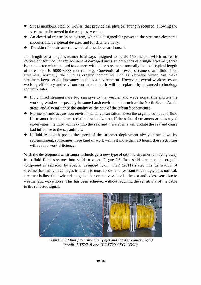
With the development of streamer technology, a new type of seismic streamer is moving away

from fluid filled streamer into solid streamer, Figure 2.6. In a solid streamer, the organic

compound is replaced by special designed foam. OGP (2011) stated this generation of

streamer has many advantages in that it is more robust and resistant to damage, does not leak

streamer ballast fluid when damaged either on the vessel or in the sea and is less sensitive to

weather and wave noise. This has been achieved without reducing the sensitivity of the cable

to the reflected signal.

Figure 2. 6 Fluid filled streamer (left) and solid streamer (right)

(credit: HYSY718 and HYSY720 GEO-COSL)

20 / 83

As the weather and the waves always affect seismic activities, the towing depth of streamers

is always designed to escape from the influence of bad weather and noise; and is also

designed according to the customers‘ demand. Normally the depth is designed within 6-10

meters.

During marine seismic acquisition, some traditional external devices are always attached on

the streamers to achieve functionality, such as the acoustic unit (figure 2.7 left up) which is

used to supply position service and compass birds (figure 2.7 down left) which are used to

control the depth of the streamer; while lateral-control birds are used to control the movement

in the horizontal direction.

Figure 2. 7 Devices attached on streamers (credit: ION geophysical)

In the end of each streamer there is a tail boy (figure 2.8) used to house Differential Global

Positioning System (DGPS) receivers that are used in the positioning solution for the

hydrophone groups in the streamers. DGPS is a standard system used for positioning the

vessel itself and relative DGPS used to position both source floats and tail buoys (OGP, 2011).

As the top right acoustic units shown in figure 2.7, these acoustic are always housed on gun

array and tail buoys, connecting with acoustic on streamer and DGPS systems, a specific

acoustic network is generated, shown in figure 2.8.

Figure 2. 8 Tailbuoy on board (left) and acoustic network (credit: HYSY720-GEOCOSL)

21 / 83

2.4.2 Seismic sources

In marine seismic acquisition activities, airgun arrays are high frequency used seismic sources.

As airgun arrays consist of sub arrays with several multiple airguns, Krail (2010) stated that

the airgun releases a high pressure bubble of air underwater as a source of energy to generate

the acoustic/pressure waves that are used in seismic reflection surveys.

One type of airgun called G. Gun 150 designed by SERCEL Company is shown in figure 2.9,

the operation of this type of airgun can be broken down into three phases: pre-fired phase; fire

phase and return phase.

Figure 2. 9 A photo of G. Gun and suspended guns

Figure 2.10（left）describes the pre-fired phase, compressed air fills up the return chamber in

the hollow shuttle to close and seal the main chamber. At the same time, the main chamber

located between the casing and the shuttle is pressurized. When the solenoid valve is

energized (figure 2.10 right), the triggering chamber is pressurized, allowing the shuttle to

unseal and the shuttle larger area to be pressurized. The lightweight shuttle quickly acquires a

high velocity before uncovering the ports. High-pressure air is then explosively released into

the surrounding water to generate the main acoustic pulse (fire phase). When the pressure

within the main chamber drops, the still fully pressurized return chamber returns the shuttle to

its pre-fired position (SERCEL, 2006).

Figure 2. 10 Pre-fired operation and fired operation of airgun (credit: SERCEL company)

22 / 83

As we know, marine seismic sources are made up of sub-arrays, so the output pressure of the

source is always proportional to the number and volume of the single airguns. The output of

the sources are always different from survey to survey, normally it is designed by customer or

client who has invested in the survey. Common surveys are always designed with 2000 to

3000 pounds per square inch (psi) pressure.

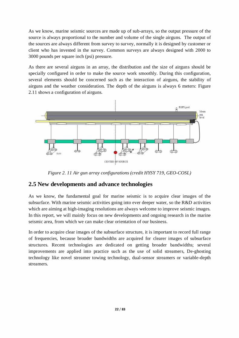
As there are several airguns in an array, the distribution and the size of airguns should be

specially configured in order to make the source work smoothly. During this configuration,

several elements should be concerned such as the interaction of airguns, the stability of

airguns and the weather consideration. The depth of the airguns is always 6 meters: Figure

2.11 shows a configuration of airguns.

Figure 2. 11 Air gun array configurations (credit HYSY 719, GEO-COSL)

2.5 New developments and advance technologies

As we know, the fundamental goal for marine seismic is to acquire clear images of the

subsurface. With marine seismic activities going into ever deeper water, so the R&D activities

which are aiming at high-imaging resolutions are always welcome to improve seismic images.

In this report, we will mainly focus on new developments and ongoing research in the marine

seismic area, from which we can make clear orientation of our business.

In order to acquire clear images of the subsurface structure, it is important to record full range

of frequencies, because broader bandwidths are acquired for clearer images of subsurface

structures. Recent technologies are dedicated on getting broader bandwidths; several

improvements are applied into practice such as the use of solid streamers, De-ghosting

technology like novel streamer towing technology, dual-sensor streamers or variable-depth

streamers.

23 / 83

2.5.1 Streamer technology improvement

A key element of this towed streamer broadband seismic technique is the streamer itself.

Dowle (2006) describes some of the recent improvements in streamer technology. The new

generation of streamer electronics can record hydrophone signals as low as 2 Hz, which add

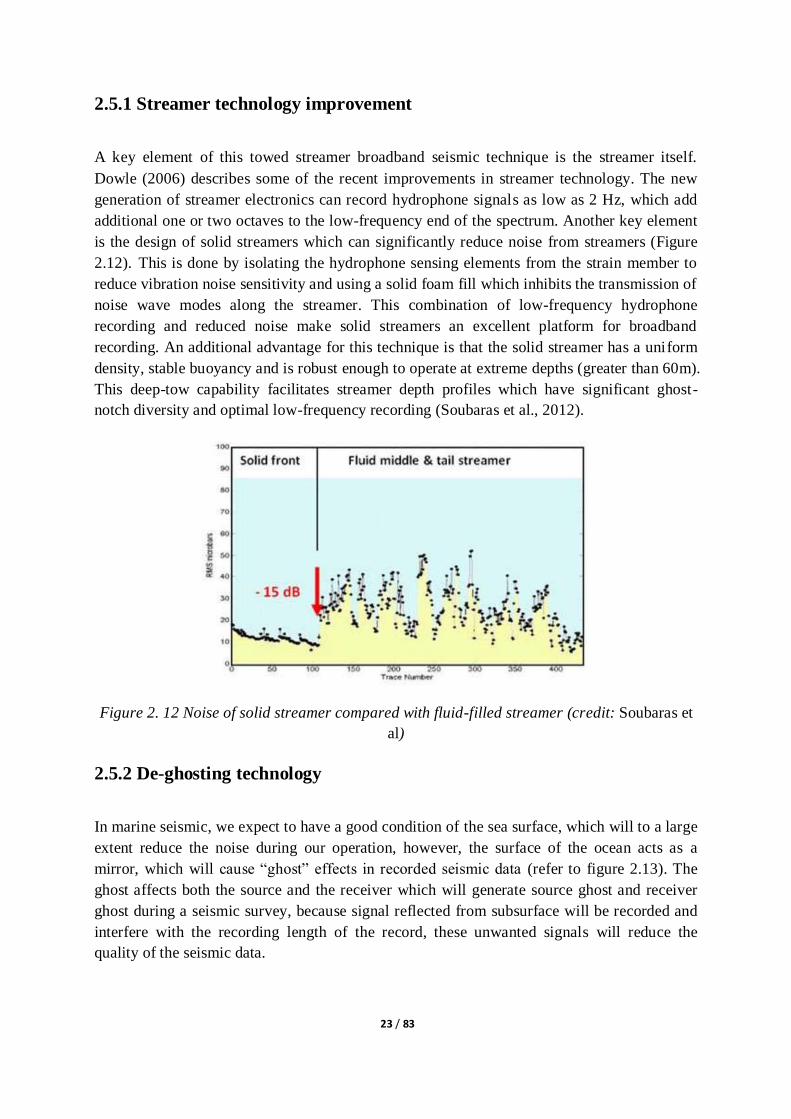
additional one or two octaves to the low-frequency end of the spectrum. Another key element

is the design of solid streamers which can significantly reduce noise from streamers (Figure

2.12). This is done by isolating the hydrophone sensing elements from the strain member to

reduce vibration noise sensitivity and using a solid foam fill which inhibits the transmission of

noise wave modes along the streamer. This combination of low-frequency hydrophone

recording and reduced noise make solid streamers an excellent platform for broadband

recording. An additional advantage for this technique is that the solid streamer has a uniform

density, stable buoyancy and is robust enough to operate at extreme depths (greater than 60m).

This deep-tow capability facilitates streamer depth profiles which have significant ghost-

notch diversity and optimal low-frequency recording (Soubaras et al., 2012).

Figure 2. 12 Noise of solid streamer compared with fluid-filled streamer (credit: Soubaras et

al)

2.5.2 De-ghosting technology

In marine seismic, we expect to have a good condition of the sea surface, which will to a large

extent reduce the noise during our operation, however, the surface of the ocean acts as a

mirror, which will cause ―ghost‖ effects in recorded seismic data (refer to figure 2.13). The

ghost affects both the source and the receiver which will generate source ghost and receiver

ghost during a seismic survey, because signal reflected from subsurface will be recorded and

interfere with the recording length of the record, these unwanted signals will reduce the

quality of the seismic data.

24 / 83

Figure 2. 13 Ghosting effect (credit: PGS)

With the development of De-ghosting technology, methodology like novel streamer towing

technology, dual-sensor streamers or variable-depth streamers are widely used by many

leading companies. The following figure 2.14 shows a configuration of a novel streamer

towing techniques operated by GEO-COSL. The deployed configuration includes a different

depth source array (6m and 12m), also with disparate streamer depth. This towing method

highly reduces attenuation and increased bandwidth. In 2009, the seismic vessels HYSY718

and HYSY719 from GEO-COSL also implemented this research which clearly demonstrated

the benefit of extending the low frequencies to improve deep imaging.

Figure 2. 14 GEO-COSL towing techniques (credit: HYSY 719, GEO-COSL)

2.5.3 More Azimuth Marine Acquisition

3D marine seismic data have traditionally been acquired by a vessel sailing in a series of

parallel straight lines. These conventional streamer surveys are called narrow azimuth, or

NAZ. This configuration suffers from an inherent problem in that the seismic ray paths are

aligned predominantly in one direction. In the presence of complex geology, salt, volcanic

layers or carbonates always exit in the overburden. Each of these so-called ―penetration

barriers‖ are associated with poor-quality seismic images contaminated with excessive noise,

and ray bending can leave portions of the subsurface untouched by seismic waves and only a

narrow range of source-receiver azimuths is recorded (WesternGeco,2012).

25 / 83

With the development of advanced acquisition techniques, acquisition methodologies such as

multi-azimuth (MAZ), wide-azimuth (WAZ), and rich-azimuth (RAZ) are widely applied to

address such illumination problems referred in narrow azimuth acquisition. Because these

advance technologies will deliver better information of subsurface structures and improve

signal-to-noise ratio during marine seismic data acquisition. In the following parts, we will

give an introduction to these methodologies.

2.5.3.1 Multi-azimuth (MAZ)

As we know, narrow-azimuth conventional surveys acquire data with one vessel with

‗racetrack‘ pattern; this kind of pattern is referencing two directions, for instance, 7°and

187°. Multiple-azimuth also uses one vessel but we acquire data in three to six directions.

The following figure 2.15 shows a typical multi-azimuth design; the survey was shot in three

complimentary azimuths, 7°, 67°and 127°.

Figure 2. 15 Multi-azimuth planned vessel tracks (credit: WesternGeco)

Howard (2007) stated that MAZ has clear operational advantages since only a single

source/recording vessel is required. It can be very cost effective because having multiple

sailing directions gives flexibility in dealing with weather, currents, waves, or temporary

surface obstructions and it eliminates the need for substantial infill. Thus, a MAZ survey with,

say, six azimuths will cost much less than six times a conventional NAZ survey. Of course, it

may cost nearly six times as much to process. In many areas, it may be a distinct advantage to

have independent conventional surveys to processes. For example, small scale anomalies can

be very difficult to resolve and build into a single velocity model, as would be required for

depth imaging.

However, MAZ still have disadvantages during marine seismic acquisition. Because even

when three to six directions‘ data are acquired, we cannot get full azimuth coverage, one

vessel sailing three to six directions will acquire repeated data, which seems not so cost

effective for a high investment project.

26 / 83

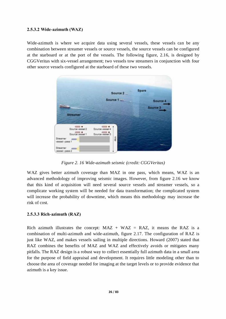
2.5.3.2 Wide-azimuth (WAZ)

Wide-azimuth is where we acquire data using several vessels, these vessels can be any

combination between streamer vessels or source vessels, the source vessels can be configured

at the starboard or at the port of the vessels. The following figure, 2.16, is designed by

CGGVeritas with six-vessel arrangement; two vessels tow streamers in conjunction with four

other source vessels configured at the starboard of these two vessels.

Figure 2. 16 Wide-azimuth seismic (credit: CGGVeritas)

WAZ gives better azimuth coverage than MAZ in one pass, which means, WAZ is an

advanced methodology of improving seismic images. However, from figure 2.16 we know

that this kind of acquisition will need several source vessels and streamer vessels, so a

complicate working system will be needed for data transformation; the complicated system

will increase the probability of downtime, which means this methodology may increase the

risk of cost.

2.5.3.3 Rich-azimuth (RAZ)

Rich azimuth illustrates the concept: MAZ + WAZ = RAZ, it means the RAZ is a

combination of multi-azimuth and wide-azimuth, figure 2.17. The configuration of RAZ is

just like WAZ, and makes vessels sailing in multiple directions. Howard (2007) stated that

RAZ combines the benefits of MAZ and WAZ and effectively avoids or mitigates many

pitfalls. The RAZ design is a robust way to collect essentially full azimuth data in a small area

for the purpose of field appraisal and development. It requires little modeling other than to

choose the area of coverage needed for imaging at the target levels or to provide evidence that

azimuth is a key issue.

27 / 83

Figure 2. 17 A RAZ survey design (credit: Howard, 2007)

28 / 83

Chapter 3 Marine seismic vessel characteristics

This chapter is intended to provide an overview of marine seismic vessels and their

characteristics. Our objective is to discuss how we can design advanced marine seismic

vessels through analyzing stability and motions due to waves within a fixed budget.

3.1 What are marine seismic vessels

Sharda (2011) stated that seismic vessels are ships that are solely used for the purpose of

seismic surveys in the high seas and oceans. A seismic vessel is used as a survey vessel for

the purpose of pinpointing and locating the best possible area for oil drilling in the middle of

the oceans.

Figure 3. 1 Seismic vessel HYSY720 from GEO-COSL

As oil drilling activities are high investment project, investors are very cautious to implement

their project without acquiring the data about the area they want to drill, because these data

that reflect the subsurface structure will give the investors‘ confidence whether they should

drill or not. In this situation, seismic vessels which are used to acquire these data are

considered critical. Besides that a seismic vessel is the one that is used to monitor the

condition of the subsurface structure.

Along with people who have strong demand for oil and gas, it is indicated that marine seismic

survey is a must, Sharda (2011) stated that in fact it can be said that every underwater

operation requires a seismic survey with the help of seismic vessels. A seismic vessel is one

of those technological developments that have the ability to enable more successes than

29 / 83

failures in fields where losses are far more costly than wins. And for this purpose alone, a

survey vessel can be regarded as the pride of modern technological invention.

3.2 Vessel characteristics

Understanding marine seismic vessels is the first step in constructing an advanced vessel, this

include general characteristics and vessel movements in the sea environment.

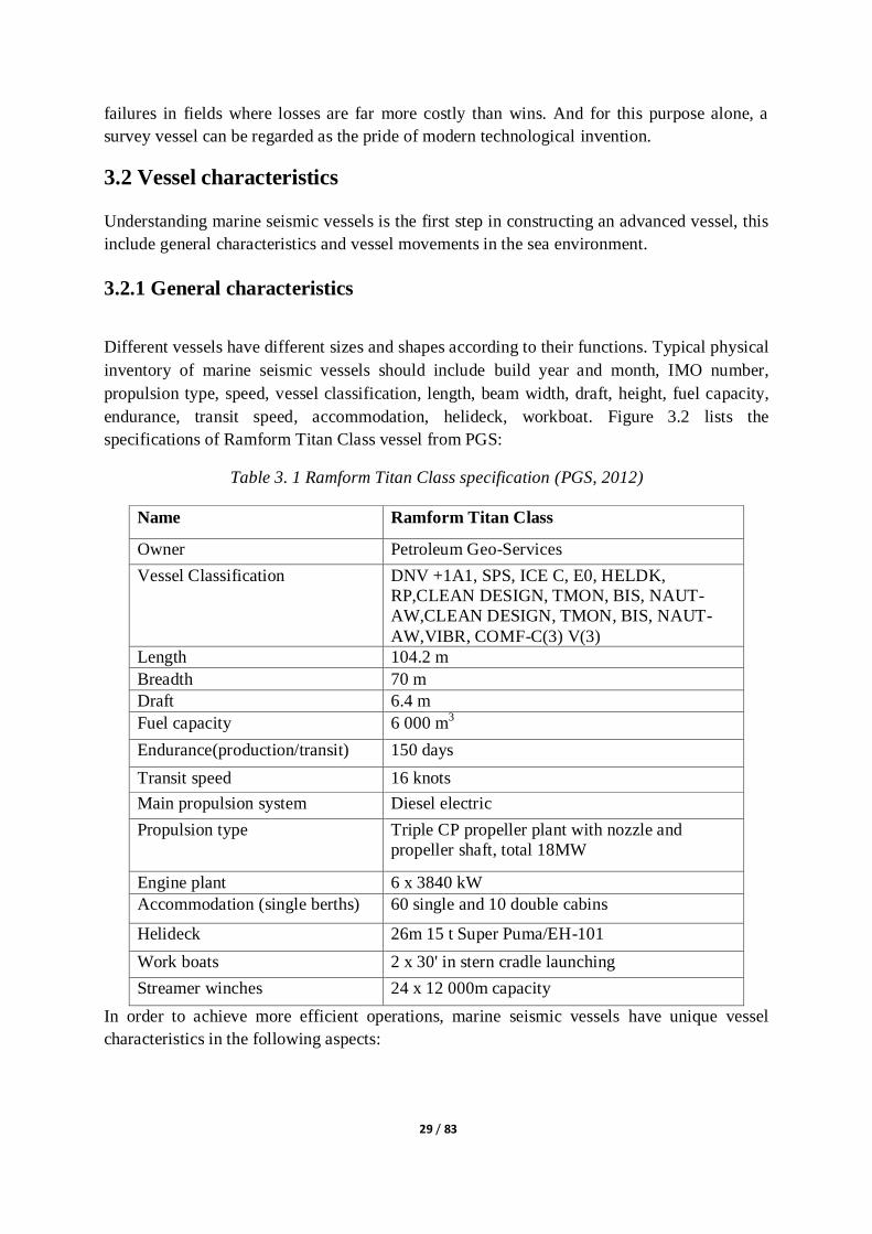
3.2.1 General characteristics

Different vessels have different sizes and shapes according to their functions. Typical physical

inventory of marine seismic vessels should include build year and month, IMO number,

propulsion type, speed, vessel classification, length, beam width, draft, height, fuel capacity,

endurance, transit speed, accommodation, helideck, workboat. Figure 3.2 lists the

specifications of Ramform Titan Class vessel from PGS:

Table 3. 1 Ramform Titan Class specification (PGS, 2012)

Name Ramform Titan Class

Owner Petroleum Geo-Services

Vessel Classification DNV +1A1, SPS, ICE C, E0, HELDK,

RP,CLEAN DESIGN, TMON, BIS, NAUT-

AW,CLEAN DESIGN, TMON, BIS, NAUT-

AW,VIBR, COMF-C(3) V(3)

Length 104.2 m

Breadth 70 m

Draft 6.4 m

Fuel capacity 6 000 m3

Endurance(production/transit) 150 days

Transit speed 16 knots

Main propulsion system Diesel electric

Propulsion type Triple CP propeller plant with nozzle and

propeller shaft, total 18MW

Engine plant 6 x 3840 kW

Accommodation (single berths) 60 single and 10 double cabins

Helideck 26m 15 t Super Puma/EH-101

Work boats 2 x 30' in stern cradle launching

Streamer winches 24 x 12 000m capacity

In order to achieve more efficient operations, marine seismic vessels have unique vessel

characteristics in the following aspects:

30 / 83

Special designed propulsion system according to the vessel towing capacity. Generally

speaking, the towing capacity is increasing with the client‘s demand.

Higher acquisition speed and transit speed to improve working efficiency and reduce

recovery time.

Higher fuel efficiency is always welcomed due to this higher investment projects.

Longer endurance and comfort accommodations onboard.

Faster streamer deployment and retrieval.

Higher reel capacity.

3.2.2 Vessel design

With offshore operation properties, marine seismic vessels are integrated and independent. In

order to work safely and orderly, equipment and facilities onboard the vessel should be laid

out regularly. The basic difference between seismic vessels and other vessels are professional

equipment or systems that are used for data acquisition; they are the streamer system, source

handling system, towing system and auxiliary system. In the following figure, a seismic

vessel designed by Rolls-Royce is shown, with detailed lay out of these systems onboard.

Figure 3. 2 Deck machinery for seismic vessels (credit: Rolls-Royce)

The streamer system and source handling system are core systems of these four systems. The

streamer system and source system are always driven by electricity or hydraulic engineering.

The streamer system is intended to deploy/retrieve streamers into/from the sea. It consists of

streamer winch, spooling device and tow point (with Fairlead Block, see figure 3.3). The

31 / 83

Source handling system is used to pick up/deploy seismic sources from/into the sea. With

implantation of science and technology into these systems, now streamer systems and source

handling systems have the ability of remote and automated operation.

Figure 3. 3 Streamer tow point (left) and paravane (right) (credit HYSY 720, GEO-COSL)

The wide tow system is typically used to deploy and retrieve paravanes (used to extend the

interval between streamers). This system mainly consists of towing winch and spooling

devices.

The auxiliary system consists of various types of equipment that complements the main

system; the auxiliary equipment can be delivered as a system and be integrated in the control

system or delivered as standalone units. The system comprises the following units: Auxiliary

winches, storage winches, spread rope winches, spooling racks, HP Air manifold, rope/wire

blocks, various types of floats, handling booms, transverse multi-purpose winches moving

vessel profiler, hydraulic power units (Rolls-Royce, 2012).

3.3 Vessel movements

A seismic vessel that is working in sea is always subject to the outer forces from winds,

waves, currents and forces from streamers and sources and other equipment in the sea water.

Generally speaking, all vessels in the sea will involve three types of linear motion: surge,

sway and heave; and three types of rotational motion: roll, pitch and yaw, these types of

motion are shown in figure 3.4. We should know that all these six types of motion are mainly

generated by sea waves.

32 / 83

Figure 3. 4 Forces working on vessel (credit: USACE National Economic Development )

From figure 3.4 we know that rolling and surging moves around X axis. Rolling happens

when waves strike the starboard or port side of the vessel, it is side to side movement; while

surging happens when waves strike one end of the vessel, the vessel will be pushed in the

direction of the wave.

Pitching and swaying moves around Y axis. Pitching happen when wave crest strike bow of

the vessel, which will cause bow is lifted and stern is lower. Pitching is a rotary movement

around Y axis. Swaying happen when wave strike the starboard side of the vessel, it will

cause the vessel move in the direction to the port side, swaying is a linear movement.

Just like we discuss four movements upside, heaving and yawing moves around Z axis.

Heaving happens when wave come from the bottom of the vessel, which make vessel moves

up with the same direction of the waves, it is a linear movement; yawing happen when waves

come from bow on starboard side, the vessel will be generated a rotary movement around Z

axis.

3.4 Marine seismic vessel stability consideration

Under any circumstance, vessel stability is a fundamental principle to guarantee that the

vessel will perform daily activity safely. Ship Hydrostatics (2002) stated that stability is the

ability of a body, in this setting a ship or a floating vessel, to resist the overturning forces and

return to its original position after the disturbing forces are removed. Actually, stability is to

balance idealized ship weight against the external forces. According to Ship Stability (1997),

these forces may arise from weather phenomena such as wind and waves, or from tow lines,

shifting of cargo or passengers, or flooding due to damage.

Most seismic vessels are used for the purpose of marine seismic survey in deep sea and

oceans. A marine seismic vessel is always special designed according to its functions. During

seismic acquisition, these vessels always tow many streamers in the sea. In order to achieve

convenient streamers deployment and retrieval, seismic vessels have wider stern than normal

vessels, (see the following figure 3.5), which make marine seismic vessels especially need

good initial stability.

33 / 83

Figure 3. 5 A marine seismic vessel (PGS, 2012)

O.T.Gudmestad (2012) has stated that initial stability is required for a small deviation from

the original position; it means that the vessel will go back to its original position when the

outer force goes away. From figure 3.1 we see that this marine seismic vessel can be

considered as a triangular vessel, in the following part I will use knowledge learned from the

Marine technology and design course at University of Stavanger to find the formula for the

initial stability of this triangular vessel.

According to DNV (one of the world‘s leading classification societies) rules for

classifications of ships, typical requirements for barge transport as shown in table 3.2, here

GM is the distance from the center of gravity to the metacenter. DNV Rules for Ships, which

announced in January 2005 demonstrated typical requirements for barge transport, see table

3.2:

Table 3. 2 Typical requirements for barge transport (DNV, 2005)

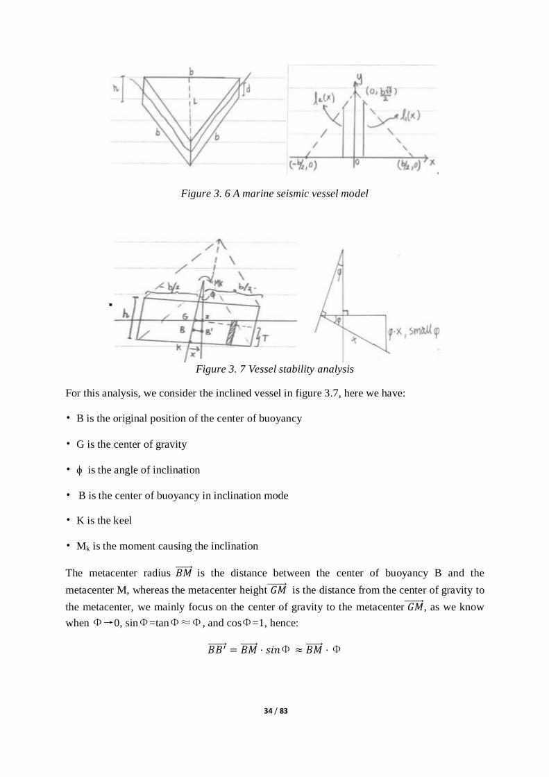
Now let us look at a vessel model shown in figure 3.6 (left), in order to achieve a simple

analysis of the initial stability of the marine seismic vessel. We assume this vessel with all

sides equal to a value b, the hull draft is d, the height is h and the total weight M, the vessel is

designed as having its weight uniformly distributed, let us try to find the formula for the initial

stability of this vessel.

34 / 83

Figure 3. 6 A marine seismic vessel model

Figure 3. 7 Vessel stability analysis

For this analysis, we consider the inclined vessel in figure 3.7, here we have:

• B is the original position of the center of buoyancy

• G is the center of gravity

• ϕ is the angle of inclination

• B is the center of buoyancy in inclination mode

• K is the keel

• Mk is the moment causing the inclination

The metacenter radius is the distance between the center of buoyancy B and the

metacenter M, whereas the metacenter height is the distance from the center of gravity to

the metacenter, we mainly focus on the center of gravity to the metacenter , as we know

when Φ→0, sinΦ=tanΦ≈Φ, and cosΦ=1, hence:

Φ Φ

35 / 83

l1(x) = √

√ , l2(x) =

√

√

First, let us consider the term ｇ ∇ , from geometry, we have that:

ｇ ∇ = ∫ √ ｇ

(

) ∫ √ ｇ

(

) =√ ｇ ∫

√ ｇ ∫

=√ ｇ

+√ ｇ

=√ ｇ

(

)

(

)

(

)

(

)

(

)

(

)

=√ ｇ

= √ ｇ

Here ∇ is the submerged volume of the vessel, we have ∇=

(

√

) =

√

So: ｇ √

√ ｇ

we get

We know

As we know, GM is the distance from the center of gravity to the metacenter, according to

typical requirements from DNV rules, if vessels transport is in open sea, after check on this

figure from the DNV roles, should meet the need that

This formulate demonstrate the relationship among draft, side and height. Design of vessel

geometry should be based on this formulate when investors want to follow DNV standard.

3.5 Vessel operational constraints

Unlike other vessels, marine seismic vessels tow amount of underwater equipment, the length

of streamers are several kilometers long, the width normally more than one kilometer, under

this condition, marine seismic vessel have some constraints during data acquisition.

36 / 83

3.5.1 Turning radius constraint

As we stated above, streamers towed behind a seismic vessel are always several kilometers

long, if the vessel need to turn to another direction, it is definitely different from other kind of

vessels; during turning, an appropriate radius is needed to help underwater equipment keep in

a safety position, that is why marine seismic data acquisition should follow a racetrack pattern.

Normally the turning radius is rough estimated according to the length of the streamers, for

example, if the streamer is 5 kilometers long, the turning radius with 2 kilometers is

appropriate.

3.5.2 Vessel speed constraint

During marine seismic acquisition activities, we ask for a faster transit speed, which will save

time for a high investment project, while to a certain extent, the acquisition speed is restrict by

a specific acquisition parameter such as a given acquisition length, too fast speed will cause

data lose.in some manual specification, acquisition speed cannot be exceed 5 knots (1knot

=1.852 kilometer/hour).

3.5.3 Ambient environment constraint

Every investor call for an ideal acquisition area during acquisition, however, deal and reality

always has a gap, almost every survey will be influenced by ambient environment, which will

slow down vessel acquisition efficiency.

Fishing activity in the survey is major challenge for data acquisition, this will highly

constraint vessel operations. If fishing activities involve in marine seismic survey, under

water equipment will be damaged if they entangle with fishing net or auxiliary equipment,

probability of physical confrontation will be increased between fishing personnel and

acquisition personnel, even acquisition personnel undertake notification to fishing personnel,

sometimes, acquisition vessel need to slow down the speed to wait fishing activities, which

will lower working efficiency.

OGP (2012) summarized that the presence of shipping in the survey can restrict vessel

operations due to physical access constraints such as proximity to harbors, data acquisition in

shipping lane area such as the English Channel, or due to excessive noise contamination from

other vessels. The effect of such vessel noise can require portions of the recorded data to be

re-recorded, which necessitates the vessel repeating a sail line. Although seismic vessels are

flagged to indicate that they are towing equipment in the water, and employ guard vessels to

try to ensure that other vessels do not sail across the submerged streamers, other vessels do

not always respond and the depth control bird have to effect and emergency dive to lower

streamer below the keel depth of the transgressing vessel when this happens, this results in

37 / 83

data acquisition having to be aborted and the vessel having to circle to re-acquire the line,

starting some distance back from where the incident occurred to ensure proper overlap of

subsurface data coverage.

Fixed obstacles such as drilling rigs or platforms in and around the survey are also constraints

for vessel operations. For these kinds of obstacles, seismic vessel has to escape from these

obstacle in order to make the underwater equipment safe, this will cause a data lose near the

obstacles

The seismic interference from other seismic vessels in ambient area is also vessel constraint

during operation. The degree of influence by seismic interference depends on the direction

and source energy of ambient vessels.

3.6 Class notation for seismic vessels

In the summer of 2012, DNV announced a new class notation for seismic vessels after

consulted with three leading geophysical companies WesternGeco, PGS and Fugro-Geoteam.

The new notation focuses on the requirement to hull arrangement and hull strength, as well as

certification requirement of system and equipment; all of these will increase the availability of

the vessels‘ operations.

The class notation has taken the DNV concept for redundant propulsion one step further so

that any failure on board will not lead to loss of more than 50 per cent forward trust. This is

sufficient to maintain a minimum speed of a few knots and will protect any high cost air guns

and streamers deployed (Richardsen, P, W., 2012).

In the new class notation, from pipe arrangement to pressure relief valves arrangement, all

parts in the high pressure systems are all given specific instructions, all of which are used to

ensure safe deck operations.

For more details about class notation for seismic vessels, please refer to appendix 2: DNV

Class notation of seismographic research vessels.

38 / 83

Chapter 4 Acquisition project management

In order to achieve an effective marine seismic data acquisition project, some project

management models are recommended. In this chapter, we mainly discuss some models used

in project initiation, procurement, operation and maintenance.

4.1 Creating a project network

During marine seismic data acquisition, many activities are involved in the project. Defining

the logical relationships between these activities will save time and budget, especially for this

high investment acquisition project. In this part, we will therefore discuss how a project

network will save time and budget in the acquisition project. We assume the duration of every

activity has already been estimated (normally we use historical data for the, time the activity

takes or we use a probabilistic method). Under this assumption, we define activity

dependencies and create a project network.

4.1.1 Sequencing activities

Gardiner, P, D (2005) suggested a method to define the logical relationships between

activities. If activities in the project are independent of each other and can be done at the same

time, these activities are sequenced in parallel (see figure 4.1(a)), if these activities are

dependent on each other and must follow one after the other, these activities are sequence in

series (see figure 4.1(b)).

Figure 4. 1 Relationship between activities (credit: Gardiner, P, D)

39 / 83

4.1.2 The network diagram

Gardiner, P,D (2005) stated that a network diagram not only shows the relationships between

activities but can be used to reveal which activities are time-critical, and so warrant greater

management attention. So a network diagram is very important for a project management.

Before we draw a network diagram, we should know that each activity should have seven

attributes as shown in figure 4.2, activity name and code, earliest start time, duration, earliest

finish time, latest start time, float/slack, latest finish time. This box which is used to display

these attributes is called the activity box.

Figure 4. 2 Standard labelling for an activity box (credit: Gardiner,P,D)

Now, there is one consideration before we draw a diagram, how many kinds of relationships

are there between activities? Totally there are four relationships between activities (for

example between A and B), they are finish-to-start; start-to-start; finish-to-finish and start-to-

finish, and the diagram of relationships is shown in figure 4.3.

Figure 4. 3 Relationships between activities (credit: Gardiner, P, D)

40 / 83

Finish-to-start means activity A must finish before activity B has permission to start; Start-to-

start means once activity A has started, activity B must also be started; Finish-to-finish means

activity A must be finished before activity B can finish; Start-to-finish means as long as

activity A has started, we can proceed to finish activity B. For these four relationships, a time

lag can be written on the arrow to indicate if there must be a delay between A and B (Gardiner,

P, D, 2005). We should know that, during marine seismic data acquisition project, Finish-to-

start relationships are the most common used relationships in the project network.

4.1.3 Creating a network

Creating a network will give managers a holistic overview of relationships between all

activities that are involved in a project, and a network will help managers to find which

activities are critical and which activities cannot be delayed, here these activities which

cannot be delayed are called ―critical activities‖.

We should know that critical activities have zero float, these critical activities generate a

critical path which have the longest duration in the network. In order to find critical activities,

the first step is to carry out a forward pass through a network, it begins from the first activity

until we reach to the last activity, and the EST of the first activity is always zero. If an activity

can be started after several activities, the EST is taken from the activity that has the highest

EFT. After finishing forward pass, we should write down EST and EFT. The EFT for the last

activity is the expected duration of the project.

After finishing the forward pass, the next step is to continue backward pass, it start from the

last activity, the LFT is equal to EFT, and the LST= LFT- duration, the float = LFT-EFT =

LST-EST.

If an activity has more than one immediate successor, the LFT is taken from the path having

the numerically lowest LST (Gardiner, P, D, 2005).

According to description above, we give an example and try to find the critical path and the

duration of the project. Assume there are eight activities involved in a project, activity H can

start when the activities E, F and G are completed. Activity D and E can start when activity B

is completed. Activity F can start when the activity C is completed, and activity G can start

when the activity D is completed. Activity B can start when A is completed, and activity C

can start 2 weeks after A is completed. The duration of each activity is given in table 4.1.

41 / 83

Table 4. 1 Duration of each activity

Activity Duration (in weeks)

A 4

B 6

C 8

D 8

E 10

F 11

G 4

H 10

With this information given above, a network diagram is shown in figure 4.4, in which the

duration is 35 weeks and the critical path is A-C-F-I.

Figure 4. 4 An activity network

Applying network diagrams in marine seismic data acquisition project will help managers

schedule and plan resources for the project, network diagrams will help managers concentrate

on managing those activities which could cause delays to the whole project.

4.2 Procurement management

Project procurement management includes the processes required to acquire goods and

services, to attain project scope, from outside the performing organization (PMI, 2000:8).

In this thesis, we mainly discuss a procurement strategy based on a life cycle cost

consideration. We will take streamer procurement as an example to illustrate LCC

procurement strategy.

In the past, comparisons of asset alternatives are mainly based on initial capital costs,

however, usually the cost of operation, maintenance, and disposal exceed all other first costs

many times over (supporting costs are often 2-20 times greater than the initial procurement

costs) (Barringer, 2003) .

42 / 83

The Life cycle cost (LCC), Figure 4.1, is the total cost of ownership of machinery and

equipment, including its cost of acquisition, operation, maintenance, conversion, and/or

decommission (SAE 1999). LCC analysis is a tool for economic analysis and engineering

analysis. It is used as a measurement and comparison tool to evaluate the life cycle cost

among all alternatives and make choices accordingly. It is a reliable method to reveal which

equipment or system is cost-effective throughout the life cycle of a project.

Figure 4. 5 Life Cycle Cost Analysis, (PMstudy, 2012)

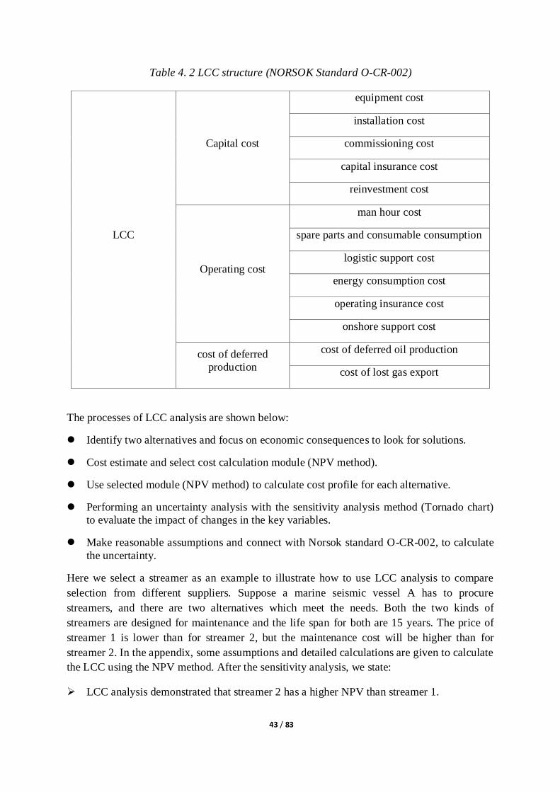
NORSOK Standard O-CR-002 clarifies three functions of LCC for production facilities:

Optimizing the production facility

System optimization during the engineering phase

Modification projects and optimization during operation

In this part, we use NORSOK Standard O-CR-002 to make a LCC analysis for the selection of

marine seismic streamers which are supplied from different suppliers. During the LCC

analysis, the Net Present Value (NPV) methodology will be used to determine which kind of

streamer is most cost effective. The Net Present Value (NPV) of an investment is the present

value (PV) of the expected cash flows, less the cost of the investment, NPV= PV- Cost. While

PV mean the present worth of a future value, it is calculate by a discount of future value,

PV=future value/discount rate.

NORSOK Standard O-CR-002 defines LCC as being equal to the sum of the operating cost,

capital cost and deferred production cost. We will apply this method to perform a LCC

analysis of a marine seismic project. Table 4.2 shows the major costs and potential loss

factors involved in the LCC analysis which are referred in NORSOK Standard O-CR-002:

43 / 83

Table 4. 2 LCC structure (NORSOK Standard O-CR-002)

LCC

Capital cost

equipment cost

installation cost

commissioning cost

capital insurance cost

reinvestment cost

Operating cost

man hour cost

spare parts and consumable consumption

logistic support cost

energy consumption cost

operating insurance cost

onshore support cost

cost of deferred

production

cost of deferred oil production

cost of lost gas export

The processes of LCC analysis are shown below:

Identify two alternatives and focus on economic consequences to look for solutions.

Cost estimate and select cost calculation module (NPV method).

Use selected module (NPV method) to calculate cost profile for each alternative.

Performing an uncertainty analysis with the sensitivity analysis method (Tornado chart)

to evaluate the impact of changes in the key variables.

Make reasonable assumptions and connect with Norsok standard O-CR-002, to calculate

the uncertainty.

Here we select a streamer as an example to illustrate how to use LCC analysis to compare

selection from different suppliers. Suppose a marine seismic vessel A has to procure

streamers, and there are two alternatives which meet the needs. Both the two kinds of

streamers are designed for maintenance and the life span for both are 15 years. The price of

streamer 1 is lower than for streamer 2, but the maintenance cost will be higher than for

streamer 2. In the appendix, some assumptions and detailed calculations are given to calculate

the LCC using the NPV method. After the sensitivity analysis, we state:

LCC analysis demonstrated that streamer 2 has a higher NPV than streamer 1.

44 / 83

Streamer 1 has lower capital cost than streamer 2, but operation cost are much higher than

for streamer 2. Man hour costs and spare parts and consumable consumption are key

factors to make the operation cost higher, higher man hour cost and needs for more spare

parts and consumable consumption means that streamer 1 will have more failures which

induce more operation and maintenance cost; and downtime costs to carry out

maintenance and repair during its lifecycle.

Tornado chart is a risk analysis method to uncover the key factors and demonstrate how

these key factors affect the LCC of the two alternatives.

Streamer 2 is more cost effective than streamer 1.

In this case study, the whole life cycle costs are considered in equipment selection, rather than

only the procurement costs. Based on a payback period, LCC analysis helps investors

maintain budgets, reduce their cost and present decision making in financial perspective to

select streamers to achieve the lowest long term cost.

4.3 Equipment maintenance technology

Maintenance costs always occupy a large propotion of the total costs during equipment

operation. Recent researches indicate that more than 30 persent of all maintenance cost are

wasted due to unconscionable maintenance technology. From this point of view, we can judge

that an advanced maintenance technology will save lots of money and will be welcomed by

all project managers. In this part, two maintennace technology are discussed to help project

managers reliazed the importance of maintenance technology.

4.3.1 Preventive maintenance

Preventative maintenance is a program of routine equipment inspections, maintenance tasks

and repairs which are scheduled to ensure that degradation of equipment is minimized. A

well-designed preventative maintenance program slightly over-maintains equipment because

scheduling is designed for the worst case operating conditions. The overall objective is to

prevent operating problems or failures, and ensure reliable operation of a facility (Okrasa, R

1997)

Figure 4.6 is a typical bathtub curve illustrates the reliability of a product. The early life

period of the bathtub curve indicates that a new machine has a high probability of failure

because of installation problems during the first stage of operation. After this initial period,

the product will be operated in a normal life period, in this period the probability of failure is

relatively low. After this normal machine life period, the probability of failure increases and

goes into the end life of wear out period.

45 / 83

Figure 4. 6 Typical bathtub curve (credit: Astrodyne and Mansfield, 2009)

All preventive maintenance management programs assume that machines will degrade within

a time frame, from the picture, we know that it represents a likelyhood of failure over the life

of an asset. For example, an acoustic CMX will normally run 6 months before it must be

replaced. Using preventive management techniques, the CMX would be removed from

service and replaced after 6 months of operation. The problem with this approach is that the

mode of operation and variables directly affect the normal operating life of machinery. The

normal life are not the same for all CMX that handles. In this exam, the CMX may not to be

replaced after 6 months. Therefore, the labor and material used to make the repair was wasted.

According to my experience, we always use preventive maintenance in our operations, and we

are trying to find advanced solutions to achieve cost effective operation in marine seismic

acquisition.

4.3.2 Predictive Maintenance

Predictive maintenance is a philosophy or attitude that, simply stated, uses the actual

operating condition of plant equipment and systems to optimize total plant operation. A

comprehensive predictive maintenance management program uses the most cost-effective

tools (e.g., vibration monitoring, thermography, tribology) to obtain the actual operating

condition of critical plant systems and based on this actual data schedules all maintenance

activities on an as-needed basis (Okrasa, 1997).

From the definition we know that predictive maintenance is a condition-based preventive

maintenance program, in order to acquire the real time condition of an equipment, some

monitoring and diagnostic techniques should be include in a comprehensive predictive

maintenance diagram, normally, these techniques include vibration monitoring, thermography,

tribology (refer to wear oil analysis and lube oil analysis), process parameters, visual

inspection, ultrasonics, and other nondestructive testing techniques. Table 4.3 highlight some

typical applications of predictive maintenance.

46 / 83

Table 4.3 Applications of predictive maintenance (credit:NASA, 2000)

Let us consider this condition based predictive maintenance applys in a marine seismic data

acquisition project, typical benifits will be included:

Estabilish a scheduled maintennace planning

Minimize equipment downtime and unexpected failures

Reduce maintenance cost and overhaul time

Optimize spare part inventory.

Increase useful life period

4.4 Maintenance interval calculation models

In practical operations, many failure caused by replacement occurs in every phase, we now

look at some models for calculating optimal maintenance intervals. We assume that

maintenance either means replacement or perfect repair; here perfect repair means the

component is as good as new after maintenance, now we will list three models to calculate

maintenance replacement intervals.

4.4.1 Age replacement model

In the ―Age replacement model‖, the component is replaced at failure, or at age u, here u is a

fix time (see following chart, figure 4.7), whichever comes first.

47 / 83

Figure 4. 7 Age replacement model(credit: Abrahamsen,2012)

If T is the lifetime of the component, the expected time between each replacement becomes:

∫

∫

∫

( ) ∫

If we assume the cost by corrective replacement (at failure) is kc, the preventive replacement

(at age u) cost is kp, the expected cost per replacement is then:

Then the expected replacement cost per time unit becomes:

K(u)=

∫

For Age replacement only old or failed components are replaced, but we must keep an over

view of all failure or replacement times.

4.4.2 The Block replacement model

For this replacement model, the component is replaced at failure and at fixed times u, 2u, 3u...,

which is shown in figure 4.8

Figure 4. 8 Block replacement model(credit: Abrahamsen, 2012)

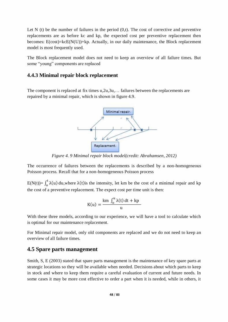
48 / 83

Let N (t) be the number of failures in the period (0,t). The cost of corrective and preventive

replacements are as before kc and kp, the expected cost per preventive replacement then

becomes: E(cost)=kcE(N(U))+kp. Actually, in our daily maintenance, the Block replacement

model is most frequently used.

The Block replacement model does not need to keep an overview of all failure times. But

some ―young‖ components are replaced

4.4.3 Minimal repair block replacement

The component is replaced at fix times u,2u,3u,… failures between the replacements are

repaired by a minimal repair, which is shown in figure 4.9.

Figure 4. 9 Minimal repair block model(credit: Abrahamsen, 2012)

The occurrence of failures between the replacements is described by a non-homogeneous

Poisson process. Recall that for a non-homogeneous Poisson process

E(N(t))= ∫

,where is the intensity, let km be the cost of a minimal repair and kp

the cost of a preventive replacement. The expect cost per time unit is then:

∫

With these three models, according to our experience, we will have a tool to calculate which

is optimal for our maintenance replacement.

For Minimal repair model, only old components are replaced and we do not need to keep an

overview of all failure times.

4.5 Spare parts management

Smith, S, E (2003) stated that spare parts management is the maintenance of key spare parts at

strategic locations so they will be available when needed. Decisions about which parts to keep

in stock and where to keep them require a careful evaluation of current and future needs. In

some cases it may be more cost effective to order a part when it is needed, while in others, it

49 / 83

is necessary to keep a spare part on hand to prevent down time in the event of breakage or

problems.

Spare parts management is used to achieve part availability when failure or wear out have

happened, effective spare parts management will face three questions: What spare parts to

store? How many spare parts to store? Where to store the spare parts? In this part, we will

solve these three problems with some models and theory.

4.5.1 What spare parts to store?

Spare parts are also called service parts, Business dictionary (2012) defines a spare part as

―Replaceable component, sub assembly, and assembly identical to and interchangeable with

the item it is intended to replace‖. Spare parts management plays a crucial role in any

organization as optimal spare parts supportability and stock levels will increase working

efficiency and to some extent reduce cost. When we decide what spare parts to store, several

factors that are involved are needed to be considered:

The criticality of item application regarding mission success.

The quantity, reliability and availability of the item.

Lead time of spare parts procurement.

Various characteristics such as the operation condition, the annual consumption value and

the unit cost.

Maintenance and inspection requirement.

The most crucial factor, the criticality of items, which is based on its function in the system,

always, specify item levels and determines what to store. Reliability and availability condition

of the production equipment/facility, when a working component will fail and need to be

replaced by a spare part. Some spare parts will be decided to store or not according to the lead

time, if the lead time is short it may be not necessary to store, however, the spare parts which

have a long lead time have to be stored to reduce the waiting time. The operation and

consumption condition will require some spare parts to be stored to meet the requirements of

operation and consumption. As well, if some overhaul or annual inspection will be

implemented, some spare parts will be required to be stored ahead of the overhaul and

inspection. The required spare parts could be standard spare parts or spare parts needed to be

manufactured according to specification.

There are several methods for classification about what spare parts to store. These are based

on the frequency of issues (FSN Analysis), the annual consumption value (ABC Analysis),

the criticality (VED Analysis), the lead time (SDE Analysis) and unit price (HML Analysis).

In marine seismic exploration, I think VED Analysis is quite appropriate, because the

criticality of items always occupies a larger weight on the decision of what spare to store.

50 / 83

In order to find out the critical items, Gajpal et al. (1994) suggested a three step hierarchy

process which is called the Analytic hierarchy process (AHP) to determine the criticality of

the items. The decision model is a breakdown structure; it is based on structuring the problem

into a hierarchy with the overall objective (or focus) at the top level 1. Criteria that are used to

evaluate the criticality of spare parts are located in the middle level 2, and the alternative

modes characterizing each of the criteria are located in the bottom level 3. For example, three

alternative of spare can be standard spare available off the shelf; standard spare but

availability not certain; non-standard spare to be fabricated according to specifications.

(Gajpal et al., 1994).

Figure 4. 10 Analytic hierarchy processes (Gajpal et al., 1994)

Based on the reliability and availability of different machines and equipment, we can classify

the items for a VED Analysis into a Vital, Essential and Desirable hierarchy, and to determine

the criticality of an item and its effect on production and other services, then we make a

classification of what spare parts to store.

4.5.2 How many spare parts to store?

Blanchard (2004) stated that ―spare parts quantities are a function of demand rates‖ and

included the consideration of the following:

1) Spare and repair parts converting actual item replacement occurring as a result of

corrective and preventive maintenance actions.

2) An additional stock level of spare parts to compensate for repairable items in the process

of undergoing maintenance.

3) An additional stock level of spare parts to compensate for the procurement lead times

required for item acquisition.

4) An additional stock level of spare parts to compensate for the condemnation or scrap age

of repairable items.

Calculation factors:

1. The reliability of items to be spared (expressed as fail, removal, replacement or inversely

as mean time between failures, MTBR, replacements).

51 / 83

2. The number of items installed.

3. The required probability that a spare part will be available when needed; normally, to

determine the quantity of spare parts, the probability P should satisfy: 90%<= P <=95%

The reliability of a system is the most important indicator of the required quantity of spare

parts, so we here focus on the calculation of system reliability. Then we calculate the quantity

of spare parts according to the result of the reliability of the system.

Fukuda, J (2008) stated that Poisson distribution is a quite frequently used forecasting

technology in spare parts quantity determination. It takes use of reliability analysis with the

following formula:

∑ [

]

Where λ=failure rate

t = time considered (or total operation period of all items involved).

x = number of failures.

λt = number of failures in time t.

Fukuda (2008) stated that spare parts can be divided in non-repairable and repairable parts.

For non-repairable parts, the number of failures equal to the number of spares. The quantity of

spare parts is the minimum value of n which satisfies the following formula:

∑ [

]

For repairable items the number of failure is different from the number of spares, because the

spares are used when the replaced items are under repair. We can apply Palm‘s theorem to

calculate

=

where MTBR means Mean Time Between Repair. For the

repairable items, the n need to be replaced by (n-1). So the formula for repairable items will

be expressed as

∑ [

]

Besides what we discussed above, Inventory system should also take into considerations

about the quantities of spare parts. An optimum balance (not too much or too little) must be

sought between the inventory on hand, the procurement frequency, and the procurement

quantity based on the budget. The following figure 4 shows the general deterministic

inventory process:

52 / 83

Figure 4. 11 Inventory considerations: (Blanchard, 2004)

The main objective of inventory considerations is to have enough amounts of spare parts to

support that a normal operational system goes smoothly versus MTTF (mean time to failure),

also to have successful repair times, and procurement lead times, and to be able to reply to

some unexpected failures and unforeseen delays. All of these activities are aiming at lowest

total cost.

Sometimes the customer satisfaction is another element of inventory consideration, because

the cost of storage will make customer satisfied in the form of short lead time and less risk of

downtime which will cost him more money.

4.5.3 Where to store the spare parts?

In offshore marine seismic industry, according to the hierarchy of the items in the VED

Analysis, it is suggested that there are three locations that will be suitable to store spare parts:

Onsite（On board or in offshore depot）: Spare parts that are vital (for frequent use and all

that with high criticality) should be stored on board to ensure normal system operation. The

onsite storage could be a decentralized storage or centralized storage. The spare parts require

some special methods to store, will be stored in a centralized way; the spare parts which are

heavy and large dimensions, not easy to transport, or required to be available at any moment

when failures occurs, will be stored in a decentralized way.

Onshore warehouse: spare parts that are essential (not so frequently used and extra parts more

than needed) could be stored in an onshore warehouse. As the onshore warehouse could

provide a better protection to the spare parts and has enough space to store large dimension

and heavy spare parts, this is also a very important method to store the spare parts. Most

onshore spare parts will be stored in the main warehouse near to the head quarter of the

53 / 83

company, but some would be stored in the warehouse close to the vessel and could easily and

quickly be transported to the vessel if needed.

Manufacturer warehouse: for the spare parts considered to be desirable (very few used but the

unavailability of which when needed would be significant), storing them in manufacturer‘s

warehouse is a good selection, these spare parts can be accessed and traced by an online

condition monitor system.

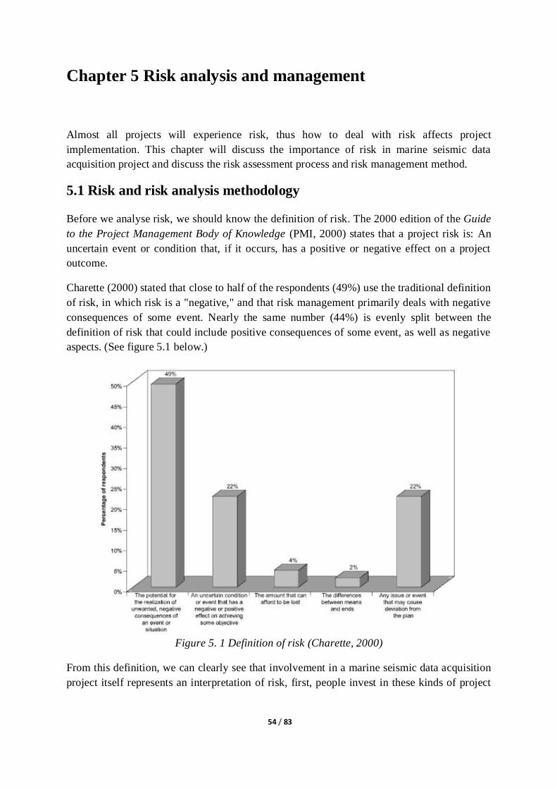
54 / 83

Chapter 5 Risk analysis and management

Almost all projects will experience risk, thus how to deal with risk affects project

implementation. This chapter will discuss the importance of risk in marine seismic data

acquisition project and discuss the risk assessment process and risk management method.

5.1 Risk and risk analysis methodology

Before we analyse risk, we should know the definition of risk. The 2000 edition of the Guide

to the Project Management Body of Knowledge (PMI, 2000) states that a project risk is: An

uncertain event or condition that, if it occurs, has a positive or negative effect on a project

outcome.

Charette (2000) stated that close to half of the respondents (49%) use the traditional definition

of risk, in which risk is a "negative," and that risk management primarily deals with negative

consequences of some event. Nearly the same number (44%) is evenly split between the

definition of risk that could include positive consequences of some event, as well as negative

aspects. (See figure 5.1 below.)

Figure 5. 1 Definition of risk (Charette, 2000)

From this definition, we can clearly see that involvement in a marine seismic data acquisition

project itself represents an interpretation of risk, first, people invest in these kinds of project

55 / 83

just like buy a stock, and the consequence will be a loss (no hydrocarbon) or a profit (find

hydrocarbon). So, an investment in a data acquisition projects have a positive or a negative

outcome, so we can consider this as a speculative risk; during project implementation, some

activities will only meet negative effects. For example, deploying streamers and guns will

only involve the chance of equipment damage in the sea, so these risks are pure negative risk.

Aven (2008) illustrate a bow-tie diagram to express the risk picture, see figure 5.2.

Figure 5. 2 An example of bow-tie diagram (based on Aven, 2008)

We can schematically describe an incident with a bow tie diagram:

The probability related events are to the left and are hindered by barriers

The possible consequences are to the right and are also hindered by barriers

The issue is then to ensure a sufficient number of barriers to hinder any possible

negative event to escalate into an unwanted consequence.

From the bow-tie diagram, we know that the risk analysis focuses on establishing a risk

picture by analyzing causes and consequences of the initiating events, in marine seismic data

acquisition project, the initiating events can be a hazard/threat which has a bad influence to

the project, or the opportunity to find a hydrocarbon structure. Some causes and consequence

barriers that effect on the initiating event are demonstrated and listed in this diagram; risk

influencing factors that are critical to the risk are also identified.

In all activities there is a risk, and in order to reduce risk to the minimum extent, we cannot

completely avoid hazard and risk during any operation, what we can do is reduce risk as much

as we can, in this condition, we introduce ALARP principle.

ALARP means the risk should be reduced to a level that is As Low As Reasonably

Practicable. This principle means that the benefits of a measure should be assessed in relation

to the disadvantages or costs of the measure. This means that an identified measure should be

implemented unless it can be documented that there is a ―gross disproportion‖ between

costs/disadvantages and benefits (Aven,2008).

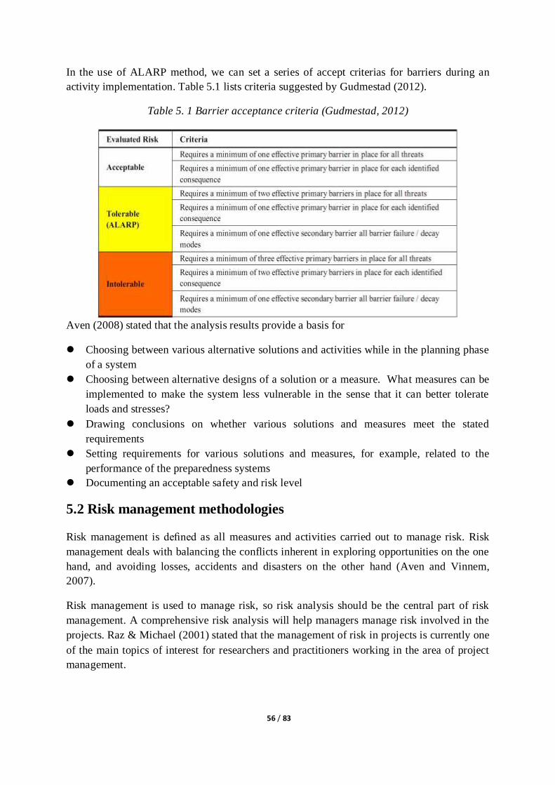
56 / 83

In the use of ALARP method, we can set a series of accept criterias for barriers during an

activity implementation. Table 5.1 lists criteria suggested by Gudmestad (2012).

Table 5. 1 Barrier acceptance criteria (Gudmestad, 2012)

Aven (2008) stated that the analysis results provide a basis for

Choosing between various alternative solutions and activities while in the planning phase

of a system

Choosing between alternative designs of a solution or a measure. What measures can be

implemented to make the system less vulnerable in the sense that it can better tolerate

loads and stresses?

Drawing conclusions on whether various solutions and measures meet the stated

requirements

Setting requirements for various solutions and measures, for example, related to the

performance of the preparedness systems

Documenting an acceptable safety and risk level

5.2 Risk management methodologies

Risk management is defined as all measures and activities carried out to manage risk. Risk

management deals with balancing the conflicts inherent in exploring opportunities on the one

hand, and avoiding losses, accidents and disasters on the other hand (Aven and Vinnem,

2007).

Risk management is used to manage risk, so risk analysis should be the central part of risk

management. A comprehensive risk analysis will help managers manage risk involved in the

projects. Raz & Michael (2001) stated that the management of risk in projects is currently one

of the main topics of interest for researchers and practitioners working in the area of project

management.

57 / 83

5.2.1 Hazard identification

Before we implement a risk analysis methodology, we should first talk about hazard

identification.

Maragakis et al. (2009) stated that Hazards identification is the act of recognizing the failure

conditions or threats (Safety Events), which could lead to Undesirable Events and defined the

characteristics of theses undesirable events in terms of their potential Safety Outcomes and of

the magnitude of these safety outcomes‘ Consequences.

Aven (2008) stated that it is difficult to avoid or to reduce the consequences of events that one

has not identified. For this reason, the identification of the initiating events (here we talk about

hazard) is a critical task of the analysis. Figure 5.3 lists the process of hazard identification,

and lists some hazard identification techniques which are based on qualitative analysis.

Figure 5. 3 Hazard identification (Aven, 2008)

In order to identify all the hazards which may occur during an operation, it is recommended to

apply methodically techniques during hazard identification. Normally, there are two kind of

methodologies used to identify hazard; they are the qualitative and quantitative risk analysis.

Investopedia US (2013) stated that qualitative analysis uses subjective judgment based on no

quantifiable information, such as management expertise, industry cycles, strength of research

and development, and labor relations. This type of analysis technique is different than

quantitative analysis, which focuses on numbers. Due to the marine operation of seismic data

acquisition projects, in this thesis, we mainly discuss qualitative analysis.

58 / 83

5.2.2 Qualitative analysis

Smith et al. (2006) state that a typical qualitative risk management usually includes the

following aspects:

A brief description of the risk;

The stages of the projects when risk may occur;

The elements of the project that could be affected;

The factors that influence risk to occur;

The relationship with other risks;

The likelihood of risk occurring;

How risk could affect the project.

In the following part, we will discuss several qualitative risk methodologies; all these risk

methodologies are based on Aven (1992).

5.2.1.1 Checklist

Checklists are lists of known hazards or hazard causes that have been derived from past

experience. The past experience could be previous risk assessments of similar systems or

operations or from actual incidents that have occurred in the past (Maragakis et al., 2009).

Checklist methodology is a previous knowledge and experience based technique, hazard that

have never happen before may be missed, and it has limitation in novel systems.

5.2.1.2 Job Safe Analysis (JSA)

JSA is usually based on checklists; it is used to identify potential hazards during every step

involved in implementing a specific job, analyzing and taking actions to make the job avert

from hazards.

Special forms are always designed for job safety analysis. In the form, potential hazards are

analyzed and measures are demonstrated in advance. JSA will help people realize that

everyone‘s safety is the first priority; job safety analysis usually decomposes a task into

several sub-tasks, and analyzes each task respectively. Table 5.2 is a typical job safety

analysis form.

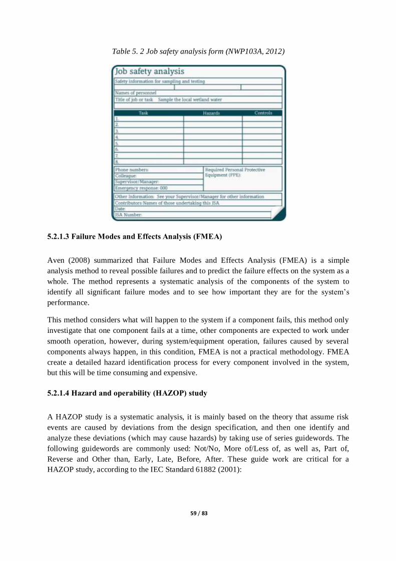
59 / 83

Table 5. 2 Job safety analysis form (NWP103A, 2012)

5.2.1.3 Failure Modes and Effects Analysis (FMEA)

Aven (2008) summarized that Failure Modes and Effects Analysis (FMEA) is a simple

analysis method to reveal possible failures and to predict the failure effects on the system as a

whole. The method represents a systematic analysis of the components of the system to

identify all significant failure modes and to see how important they are for the system‘s

performance.

This method considers what will happen to the system if a component fails, this method only

investigate that one component fails at a time, other components are expected to work under

smooth operation, however, during system/equipment operation, failures caused by several

components always happen, in this condition, FMEA is not a practical methodology. FMEA

create a detailed hazard identification process for every component involved in the system,

but this will be time consuming and expensive.

5.2.1.4 Hazard and operability (HAZOP) study

A HAZOP study is a systematic analysis, it is mainly based on the theory that assume risk

events are caused by deviations from the design specification, and then one identify and

analyze these deviations (which may cause hazards) by taking use of series guidewords. The

following guidewords are commonly used: Not/No, More of/Less of, as well as, Part of,

Reverse and Other than, Early, Late, Before, After. These guide work are critical for a

HAZOP study, according to the IEC Standard 61882 (2001):

60 / 83

The identification of deviations from the design intent is achieved by a questioning process

using predetermined ―guide words‖. The role of the guide word is to stimulate imaginative

thinking, to focus the study and elicit ideas and discussion.

The main job of HAZOP is analyzing the causes and consequences of these deviations. The

procedure of a HAZOP can be illustrated in the following figure 5.4.

Figure 5. 4 A HAZOP procedure (Rausand, 2005)

5.2.1.5 Structured What-If Technique (SWIFT)

SWIFT is a systematic technique for hazard identification. It is just like HAZOP, it is also

using predefined checklists to identify deviations from normal operations, SWIFT analyze

deviations from normal operation is based on brainstorming, it is beginning with ―what if‖

and ―how could‖. It relies on a higher level the opinions from experts to identify hazard.

In a word, all these five qualitative methods are cost effective methodologies for hazard

identification, we can also consider these methods as risk reduction methods. According to

DNV-OSS-121:

The results of hazard identification and evaluation present a good opportunity for targeted

risk reduction. In assigning classification, DNV expects that such risk reduction will be

undertaken wherever significant and practicable opportunities are identified.

Hazard identification and evaluation is most effectively initiated at concept design stage

where risks can be avoided or reduced. For existing installations where this is not possible,

hazard identification and evaluation should be used to address hazards and optimising the

protection measures to manage them. In order of importance, this means measures to prevent,

detect, control and mitigate against hazards.

61 / 83

5.3 Risk involved in marine seismic exploration

An investment in data acquisition projects is an activity with speculative risk, although marine

seismic data acquisition projects themselves are risk reduction measures for oil drilling

projects, implement these projects always involve different kinds of hazards or risks. In this

part, the mainly risks involved in data acquisition projects are discussed in details.

5.3.1 Personnel operational risk

Joshi (2012) stated that a good survey design, technology, resources (equipment, software,

and hardware), financial back up etc. can be easily ruined by deputing non suitable personnel

in the key position and there is no way to cover up this risk once the project is complete.

Personnel at every stage of the job always play a crucial role in the life cycle of a project,

especially in a complicated working environment.

From 1993 to 1997, UKOOA (1998) as cited in Nick &Gatwick (1999) stated that an

investigation relating to LTI (Lost Time Injuries) in marine seismic business demonstrated

that the back deck operations are the most hazardous work area, see table 5.2. The reason

being that although air-gun deck and streamer decks are designed in different floors, some

deflector systems are mixed with numerous towing winches and handling systems. At the

same time, personnel is challenged to deploy and operate an increasing number of auxiliary

equipment packing on the streamers, that is why back deck operation occupy such a big

proportion of risk.

Table 5. 3 Lost Time Injuries by work area (Nick &Gatwick, 1999)

In order to eliminate operational risk during marine seismic business, a HAZOP can be used

as a risk reduction methods, Swinstead (2004) suggested several principles to undertaken:

Eliminate safety hazards with the work area by redesigning deployment equipment and

working practices. Such as: a dynamic streamer tow-point system, which will retract and

lower streamers to a comfortable operation; taking use of remote control device to make

a safety distance between human and equipment.

Only standard and certified equipment is accepted for the whole fleet.

62 / 83

Improve training methods so that potentially hazardous situations can be anticipated and

acted upon before they arise.

Improve communications between the back deck environment and the navigation and

data acquisition activities undertaken in the instrument room, also the bridge.

Standard operation regulations should be established and enforced.

Seismic vessels back deck should be divided into different areas according to function

and all these areas should be marked clearly.

Operators in the instrument room should have a holistic overview of the back deck

operation.

5.3.2 Environmental risk

During marine data acquisition, towed streamers and airguns will be deployed into the water;

personnel will live and work on board the vessel; there are also some chase boats and supply

vessels work in the survey, all of these will increase the risk to the environment, the main

potential hazard associated with the projects include:

Fuel and oil leakage from seismic vessel and equipment.

Seismic sources that cause physical disturbance to biota such as marine mammals, turtles,

fishes and sharks.

Interference with commercial fishing activities.

Garbage disposal to marine environment.

Refuel activities that could pollute the water.

Risk of introducing marine pests into the water.

In order to mitigate operation risk to the environment, we introduce the ALARP process to

reduce risk. Figure 5.5 illustrates the principle of ALARP.

Figure 5. 5 Risk matrix – balloon diagram ( Odland, 2009b)

with the ALARP principle, measures and activities should be implemented to achieve risk As

Low As Reasonably Practicable. Table 5.3 lists some activities to protect the environment

during 3D seismic data acquisitions.

63 / 83

Table 5. 4 Environment protection based on ALARP (Apache Energy Ltd, 2011)

Activity Requirement

Operational

Environmental

Awareness

Through inductions and educational material present on the

vessels, ensure that all personnel are familiar with the

environmental requirements of the environment plan to ensure

these guidelines and procedures are being followed.

Ensure all personnel sign off on the vessel register book

confirming their induction.

Minimize risk of

adverse effect to

marine biota and the

marine environment.

―Soft start‖ procedures and Interaction procedures in place

and adhered to.

Supply vessel used to assist in keeping watch for whales

Responsibilities for monitoring, responding to and recording

challenging sightings clearly identified and conveyed to vessel

personnel.

Deck drainage,

Liquid Discharges

chemical storage and

management

All discharges, including sewage, black and grey water, brine,

cooling water, bilge, ballast water, deck drainage, to comply

with legal requirements, including MARPOL (Maritime

Agreement Regarding Oil Pollution) Regulations

Maintain good housekeeping practices.

Store chemicals in enclosed areas away from open drains and

chemical containers are to be intact.

Use drip trays under all machinery and fuel points and valves.

In the event of a spill, take all actions to control the spill and

divert deck drainage to on board containment tanks for

treatment through the oil in water separator.

Ensure absorbent material is on board to use in soaking up

chemical or oil spills on deck.

Maintain oil water separators regularly to ensure 15 ppm oil

concentration alarm is functional, in accordance with

MARPOL 1973/78 requirements.

Sewage discharge Treat sewage to secondary level prior to discharge through the

sewage plant (aerates, macerates and chlorinates).

Sewage facilities to meet MARPOL 1973/78 requirements.

Maintain the sewage treatment plant in order to ensure

effective treatment.

Solid waste

management :

Food scraps

(including

putrescible

galley waste)

Garbage, Litter

Scrap metal and wood etc.

Disposal of food scraps in accordance with MARPOL

1973/78

–no disposal of un-macerated food within 12 nm from coast

Do not dispose of debris, garbage or litter into the sea (ships

need covers to prevent wind-blown rubbish – especially

plastics and cups).

Segregate industrial waste (scrap metals / drums etc.)

wherever possible for appropriate disposal onshore.

Do not use polystyrene cups.

Reduce, reuse and recycle waste wherever practicable.

Record the volume and type of waste taken off vessels and

forward to the Environmental Department at the end of the

64 / 83

seismic survey.

Minimize risk of

introducing marine

pests into surveyed

waters

Vessel log book records a full ballast water exchange at sea

prior to entry into Australian waters.

Compliance with National Biofouling Management

Guidelines for Commercial vessels and National biofouling

management guidance for the petroleum production and

exploration industry.

Maintain air quality Include inspections and tuning of engines and equipment on a

regular maintenance schedule.

Verify that vessel procedures comply with requirements of

MARPOL.

5.3.3 Weather risk

No one will deny that weather is one of the most common risks in marine seismic operations;

a better weather condition will increase the work window of marine operations. It is clear that

acquisition in areas with typhoons or monsoons have lower working efficiency than area

without them, because weather will reduce the data quality and generate delays to the working

plan. For a contract where the clients do not pay for the standby caused by weather condition,

weather influence is an indirect way to increase survey cost. So before implement an

acquisition project, an SWIFT should be discussed and analyzed regarding what will be the

consequences if bad weather exists in and around the survey area.

5.3.4. Supply chain risk

Smooth supply chain activities among suppliers and receivers are used to ensure profitability

and continuity of a specified project. Events caused by supply chain risk always bring

substantial negative consequence to the system. Tang and Nurmaya Musa (2011) summarized

several risks may happen in the supply chain:

Material flow risk. When we talk about material flow risk, the first disaster come into our

mind is Ericsson‘s inability of reacting to a supplier‘s fire accident is the consequence of

single sourcing risk (Peck et al., 2003). In order to avert this single sourcing risk, many

companies turn to multi-suppliers. However, when we switch suppliers between different

suppliers, changing supplier will also bring new risk in to the system.

Financial flow. Financial flow risk involves the inability to settle payments and leads to

improper investment. The common risks are exchange rate risk, price and cost risk,

financial strength of supply chain partners and financial handling/practice.

Information risk. Supply activities are always triggered by the information transmission

between suppliers and users, we should make sure the information is accurate during

decision making in supply chain.

65 / 83

In order to reduce supply risk in marine seismic acquisition activities, a cost-benefit method

which is based on NPV (Net Present Value) consideration will be helpful in decision making.

In appendix 1 we show a clear LCC analysis under the NPV methodology.

66 / 83

Chapter 6 Conclusions and Recommendations

A marine seismic exploration project is a high investment project with complex procedures.

In order to achieve a cost effective project, methods concerned with how to reduce cost and

improve working efficiency is appreciated by every project manager and operator. The thesis

only covers a few aspects related to marine seismic vessel design, management models and

risk reduction measures.

As the marine seismic exploration goes into deeper waters, advanced technologies are

required to meet the needs, and narrow azimuth acquisition methods will be replaced sooner

or later. Advanced technologies such as broadband, WAZ, MAZ and RAZ will be the

predominant methodologies in the future. Besides these methodologies, high volume air guns,

longer streamers, and novel streamer towing technology, dual-sensor streamers or variable-

depth streamers will be widely applied in practice.

Seismic vessels are the main vehicles for the marine seismic data acquisition project, for

towing of equipment in the water, for handling of systems and for supply of accommodations

for personnel and so on. Due to the high investment, special designed vessels should focus on

absolute safety and high working efficiency. In this thesis, a detailed stability analysis of a

marine seismic vessel is discussed. Special vessel characteristics are discussed under the

consideration of some operational constraints.

Marine seismic data acquisition projects always include plenty of activities, a network

diagram is recommended to achieve an easy management plan. LCC analysis, minimal repair

block model and the VED analysis model are recommended to achieve a cost-effective project

management.

Risk in marine seismic acquisition projects may bring disasters as acquisition activities are

always far away from the land; thus, identifying hazard in advance will reduce the probability

of bad consequences, five qualitative risk analysis methodologies are recommended in

managing risk involved in marine seismic acquisition projects.

With the acquisition activities going into deeper water and more complex environment,

further study should also focus on technology and management of harsh environment

operations, such as operations in arctic areas.

67 / 83

References

Abrahamsen, E, B., 2012. Reliability analysis, MOS 190. Optimal maintenance interval. Lectures at

University of Stavanger, unpublished.

Apache Energy Ltd, 2011. Cambozola 3D Marine Seismic Survey Environment Plan: Public Summary.

Online Available:

http://www.dmp.wa.gov.au/documents/30620_APACHE_Cambozola_3D_MSS_EP_Summary.pdf

[Accessed Jan 19th, 2013].

Astrodyne, J, B & Mansfield, M, 2009. MTBF and power supply reliability. Online Available:

http://www.electronicproducts.com/Power_Products/AC_DC_Power_Supplies/MTBF_and_power_su

pply_reliability.aspx [Accessed Oct 10th, 2012].

Aven,T.(1992)ReliabilityandRiskAnalysis.Elsevier,London.

Aven, T, 2008. Risk analysis: assessing uncertainties beyond expected values and probabilities.

Chichester: John Wiley.

Aven,T.and Vinnem,J.E., 2007. RiskManagement,with Applications from the Offshore Oil and Gas

Industry.Springer Verlag, NewYork, NY.

BARRINGER, H. P. A life cycle cost summary. International Conference of Maintenance societies, 2003.

Online Available: http://www.barringer1.com/pdf/LifeCycleCostSummary.pdf . [Accessed Oct 10th,

2012].

BLANCHARD, B. S., 2004. Logistics engineering and management. Prentice Hall, New Jersey.

British Standard, IEC Standard 61882, 2001. Hazard and operability studies (HAZOP studies) —

Application guide. Available online: http://zh.scribd.com/doc/23637115/BS-IEC-61882-2001-HAZOP-

guide [accessed Jan 12th,2013]

Business Dictionary, 2012. Spare parts definition. WebFinance, Inc., Available:

http://www.businessdictionary.com/definition/spare-part.html. [Accessed June 10th, 2012].

Charette, R., 2000. What exactly is risk management? Online Available:

http://www.cutter.com/press/020606.html [Accessed Jan 10th, 2013].

CGGVeritas,2012. Seismic overview. Online avialiable:

http://www.cggveritas.com/popup_page.aspx?cid=1-24-143 [Accessed Nov 15th, 2012].

CREWS, M. Seismic Operations in Environmentally Sensitive Areas. SPE Health, Safety and Environment in Oil and Gas Exploration and Production Conference, 1994.

http://www.dmp.wa.gov.au/documents/30620_APACHE_Cambozola_3D_MSS_EP_Summary.pdf

http://www.electronicproducts.com/Power_Products/AC_DC_Power_Supplies/MTBF_and_power_supply_reliability.aspx

http://www.electronicproducts.com/Power_Products/AC_DC_Power_Supplies/MTBF_and_power_supply_reliability.aspx

http://www.barringer1.com/pdf/LifeCycleCostSummary.pdf

http://zh.scribd.com/doc/23637115/BS-IEC-61882-2001-HAZOP-guide

http://zh.scribd.com/doc/23637115/BS-IEC-61882-2001-HAZOP-guide

http://www.businessdictionary.com/definition/spare-part.html

http://www.cutter.com/press/020606.html

http://www.cggveritas.com/popup_page.aspx?cid=1-24-143

68 / 83

DNV- Rules for Ships, January 2005 Pt,3 Ch.3 Sec.9 - Page 73. Hull equipment and safety. Online

avialiable: http://exchange.dnv.com/publishing/rulesship/2005-01/ts303.pdf [Accessed Feb 19st,

2013].

DNV Rules for Ships, July 2012, Pt.5 Ch.7 Sec.24 Class notation for of seismographic research vessels.

Online avialiable: http://exchange.dnv.com/publishing/rulesship/2012-07/ts507.pdf [Accessed Jan

15th, 2013].

DNV OFFSHORE SERVICE SPECIFICATION. DNV-OSS-121,2008. Classification Based on Performance

Criteria Determined from Risk Assessment Methodology. Online avialiable:

http://exchange.dnv.com/publishing/codes/ToC_edition.asp [Accessed Jan 16th, 2013].

Fukuda, J. 2008. SPARE PARTS STOCK LEVEL CALCULATION. Available:

http://www.geocities.ws/riekonissi/spareparts.pdf [Accessed June 15th, 2012].

GAJPAL, P. P., GANESH, L. & RAJENDRAN, C. 1994. Criticality analysis of spare parts using the ath

nalytic hierarchy process. International Journal of Production Economics, 35, 293-297.

Gardiner,P,D., 2005. Project management. London, PALGRAVE MACMILLAM, UK.

GJESTRUM, E. & SIMON, J. Accident Risk Reduction on the Back Deck of Seismic Vessels. SPE Health, Safety and Environment in Oil and Gas Exploration and Production Conference, 1994.

Gudmestad, O.T., 2012. Marine Technology and Design, MOM 480 Stability of ships and floating

vessels. Lectures at University of Stavanger, unpublished.

Howard, M. 2007. Marine seismic surveys with enhanced azimuth coverage lessons in survey design

and acquisition. [Online]. Available:

http://www.slb.com/~/media/Files/westerngeco/resources/articles/2007/apr07_tle_marine.pdf

[Accessed Nov 12th,2012]

IAGC, 2002. An overview of marine seismic operations. Available online:

http://www.iagc.org/files/306/ . [accessed Nov 12th,2012]

Investopedia US, 2013. Definition of 'Qualitative Analysis'. [Online]. Available:

http://www.investopedia.com/terms/q/qualitativeanalysis.asp#axzz2LEWb5UQp . [accessed Feb

12th,2013]

Joshi,M., 2012. Risk assessement & Business Issues In Planning 2D/3D Marine Seismic Surveys From

E&P Operator(Oil Company) Perspective. [Online]. Available: http://www.veritasearth.com/risk-

assessment-business-issues-in-planing-2d3d-marine-seismic-surveys-from-e-p-operator%E2%80%99s-

oil-company-perspective/[accessed Feb 19th,2013]

Krail, P.M., 2010. Airguns: theory and operation of the marine seismic source. Course notes for GEO-

391 Principles of seismic data acquisition, University of Texas at Austin

Maragakis et al., 2009. Safety management system and safety culture working group (SMSWG)

Guidance on hazards identification. [Online]. Available: http://easa.europa.eu/essi/ecast/wp-

http://exchange.dnv.com/publishing/rulesship/2005-01/ts303.pdf

http://exchange.dnv.com/publishing/rulesship/2012-07/ts507.pdf

http://exchange.dnv.com/publishing/codes/ToC_edition.asp

http://www.geocities.ws/riekonissi/spareparts.pdf

http://www.slb.com/~/media/Files/westerngeco/resources/articles/2007/apr07_tle_marine.pdf

http://www.iagc.org/files/306/

http://www.investopedia.com/terms/q/qualitativeanalysis.asp#axzz2LEWb5UQp

http://www.veritasearth.com/risk-assessment-business-issues-in-planing-2d3d-marine-seismic-surveys-from-e-p-operator%E2%80%99s-oil-company-perspective/



http://easa.europa.eu/essi/ecast/wp-content/uploads/2011/08/ECASTSMSWG-GuidanceonHazardIdentification1.pdf

69 / 83

content/uploads/2011/08/ECASTSMSWG-GuidanceonHazardIdentification1.pdf [accessed Feb

12th,2013]

NASA, 2000. Reliability Centered Maintenance Guide for Facilities and Collateral Equipment. National

Aeronautics and Space Administration, Washington, D.C.

Nick & Gatwick, 1999. A better way to work. [Online]. Available:

http://www.slb.com/~/media/Files/resources/oilfield_review/ors99/aut99/better.pdf [accessed Feb

19th,2013]

NWP103A,2012. Job safety analysis. [Online]. Available:

http://toolboxes.flexiblelearning.net.au/demosites/series11/11_04/toolbox_11_04/uoc3/html/p4saf

e_jsa.htm [accessed Feb 12th,2013]

NORSOK standard, O-CR-002, Rev. 1, April 1996. Standard Norway, Oslo, Norway

OGP, 2011. An overview of marine seismic operations. [Online]. Available:

http://entry.ogp.org.uk/pubs/448.pdf. [Accessed Nov 12th,2012]

Okrasa, R 1997. ELECTRICAL SYSTEMS PREVENTIVE MAINTENANCE Handbook. 2nd edition. 700

University Avenue, H10-F18 Toronto, Ontario Hydro.

Odland, J., 2009a. Offshore Field Development. MOK120, Module 4-Exploration and reserves

Replacement. Lecture notes at University of Stavanger, unpublished.

Odland, J., 2009b. Offshore Field Development. MOK120, Module 19-Economic analyses. Lecture

notes at University of Stavanger, unpublished.

Peck,H., Abley,J., Christopher,M., Haywood,M., Saw,R., Rutherford,C., Strathern,M., 2003. Creating

Resilient Supply Chains.. Cranfield University,Cranfield School of Management, UK.

PMI, 2000. Guide to the project management body of knowledge, project management institute,

Pennsylvania.

PMstudy, 2012. Life cycle cost. [Online]. Available: http://pmstudy.com/blog/?p=286 [accessed Feb

12th,2013]

Rausand, M, 2005. HAZOP, Hazard and Operability Study. [Online]. Available:

http://frigg.ivt.ntnu.no/ross/slides/hazop.pdf [accessed Feb 17th,2013]

Raz, T., & Michael, E. (2001). Use and benefits of tools for project risk management. International

Journal of Project Management, 19(1), 9-17.

Richardsen, P, W., 2012. New class notation for seismic vessels. [Online]. Available:

http://www.dnv.com/press_area/press_releases/2012/new_class_notation_for_seismic_vessels.asp

[Accessed Jan 12th,2013]

http://easa.europa.eu/essi/ecast/wp-content/uploads/2011/08/ECASTSMSWG-GuidanceonHazardIdentification1.pdf

http://www.slb.com/~/media/Files/resources/oilfield_review/ors99/aut99/better.pdf

http://toolboxes.flexiblelearning.net.au/demosites/series11/11_04/toolbox_11_04/uoc3/html/p4safe_jsa.htm

http://toolboxes.flexiblelearning.net.au/demosites/series11/11_04/toolbox_11_04/uoc3/html/p4safe_jsa.htm

http://entry.ogp.org.uk/pubs/448.pdf

http://pmstudy.com/blog/?p=286

http://frigg.ivt.ntnu.no/ross/slides/hazop.pdf

http://www.dnv.com/press_area/press_releases/2012/new_class_notation_for_seismic_vessels.asp

70 / 83

Rigzone,2012. How Does Marine Seismic Work? [Online]. Available:

http://www.rigzone.com/training/insight.asp?i_id=303 . [Accessed Nov 12th,2012]

Rolls-Royce,2012., Deck machinery for seismic vessels. Online avaiable at: http://www.rolls-

royce.com/marine/products/deck_machinery/dm_offshore/dm_siesmic/ [Accessed Nov 12th,2012]

(SAE)Society of Automotive Engineers, Reliability and Maintainability Guideline for Manufacturing

Machinery and Equipment, M-110.2, Warrendale, PA (1999)

Sercel Company,2006., Marine source. [Online]. Available:

http://www.oceandata.co.kr/GroupWare/Home/product/brochure/Sercel/Marine%20Sources.pdf

Accessed Nov 12th,2012]

Sharda, 2011. What are Seismic Vessels? [Online]. Available:

http://www.marineinsight.com/marine/types-of-ships-marine/what-are-seismic-vessels/ [Accessed

Sep 10th 2012]

Ship Hydrostatics, 2002 [Online].

Available:http://web.nps.navy.mil/~me/tsse/NavArchWeb/1/module7/basics.htm# [Accessed Sep

10th 2012]

Smith, N. J., Merna, T., & Jobling, P. (2006). Managing risk in construction projects. Oxford: Blackwell.

Smith, S.E, 2003. What is spare parts management. [Online]. Available:

http://www.wisegeek.com/what-is-spare-parts-management.htm#did-you-know [Accessed Sep 10th

2012]

Ship Stability, 1997. [Online]. Available: http://www.ghsport.com/stab.htm [Accessed Sep 10th 2012]

Soubaras, R., Whiting, P.,West, B,V., Taylor, R., 2012. Broadband marine seismic – Breaking the limits.

Online available at http://www.cggveritas.com/technicalDocuments/cggv_0000010082.pdf

[accessed Nov 12th,2012]

Swinstead,N., 2004. Human factors impact on risk analysis of complex systems. SPE Health, Safety

and Environment in Oil and Gas Exploration and Production Conference.

Tang,C.S.,2006a. Perspectives in supply chain risk management. International Journal of Production

Economics 103 (2006), 451–488.

TANG, O. & NURMAYA MUSA, S. 2011. Identifying risk issues and research advancements in supply

chain risk management. International Journal of Production Economics, 133, 25-34.

UPSeis, 2012.What is seismology and what are seismic waves? Online available at

http://www.geo.mtu.edu/UPSeis/waves.html [accessed Nov 12th,2012]

WesternGeco, 2012. Coil Shooting. Online avaiable at:

https://slb.com/services/westerngeco/services/marine/techniques_enabled/coilshooting.aspx

[Accessed Nov 12th,2012]

http://www.rigzone.com/training/insight.asp?i_id=303

http://www.rolls-royce.com/marine/products/deck_machinery/dm_offshore/dm_siesmic/

http://www.rolls-royce.com/marine/products/deck_machinery/dm_offshore/dm_siesmic/

http://www.oceandata.co.kr/GroupWare/Home/product/brochure/Sercel/Marine%20Sources.pdf

http://www.marineinsight.com/marine/types-of-ships-marine/what-are-seismic-vessels/

http://web.nps.navy.mil/~me/tsse/NavArchWeb/1/module7/basics.htm

http://www.wisegeek.com/what-is-spare-parts-management.htm#did-you-know

http://www.ghsport.com/stab.htm

http://www.cggveritas.com/technicalDocuments/cggv_0000010082.pdf

http://www.geo.mtu.edu/UPSeis/waves.html

https://slb.com/services/westerngeco/services/marine/techniques_enabled/coilshooting.aspx

71 / 83

Appendix 1: LCC analysis

Table A1.1 BASIC ASSUMPTIONS FOR STREAMER 1 and STREAMER 2

BASIC ASSUMPTIONS FOR STREAMER 1 and STREAMER 2

Streamer 1 Streamer 2

investment year 2012 2012

start of production 2013 2013

operating hours per year 8400 8520

Man hour cost 60000 16000

cost of deferred production per hour 7000 7000

spare parts and consumable consumption 40000 10000

discount rate 10% 10%

streamer life span (years) 15 15

cost of fuel per kW+CO2 tax cost per kW 0.6 0.3

We assume the power requirement is equal each year, the unit is NOK

The formula to calculate average annual energy consumption cost of single equipment is

shown as below:

Annual average energy consumption= power requirement*time in operation*cost of power

Table A1.2 Annual average energy consumption calculation

Streamer 1 Streamer 2

power requirement (kW) 3 4

operation time per year (hours) 8400 8520

cost of power (NOK/kWhour) 0.6 0.3

average annual average energy consumption (kW) 15120 10224

The formula for production loss on the streamer is as follows:

PLt=E*p*L*D Where:

PLt =Production loss in year t

E=average number of critical failures per year

72 / 83

p=probability of production reduction

L=quantity of production loss per time unit

D= duration of production reduction

Table A1.3 Cost of deferred production calculation

streamer1 streamer2

E 0.2 0.2

p 5% 5%

D ( hours) 360 240

L 0.8 0.8

PL 2.88 1.92

cost of deferred production

(NOK) 20160 13440

Evaluate the economic consequences of streamer 1 with LCC analysis.

Table A1.4 LCC analysis for streamer 1

LCC

For streamer 1 Detail cost Year 2012 Year 2013-2027

Capital cost (NOK)

equipment cost -1500000

installation cost -200000

commissioning cost -100000

insurance cost -50000

reinvestment cost -150000

Operating cost

(NOK)

man hour cost -60000

spare parts and

consumable consumption -40000

logistic support cost -10000

energy consumption cost -15120


onshore support cost -25000

Cost of deferred

production (NOK) -20160

Total cost per year -200280

Discount rate (10%) 0.1

PV -2000000 -1523345.604

LCC -3523345.6

Then we will use a Tornado Chart to determine how changes in key variables impact LCC,

and evaluate how the variables influence the LCC when they increase/ decrease by 10%.

73 / 83

Table A1.5 OPEX decrease and increase 10%

OPEX decrease 10% OPEX increase 10%

capital insurance cost (NOK) -5000 5000

logistic support cost (NOK) -7606.1 7606.08

commissioning cost (NOK) -10000 10000

energy consumption cost (NOK) -11500.4 11500.4

reinvestment cost (NOK) -15000 15000

cost of deferred production (NOK) -15333.85 15333.86

onshore support cost -19015.2 19015.2

installation cost -20000 20000

operation insurance cost -22818.23 22818.24

spare parts and consumable consumption -30424.31 30424.32

man hour cost -45636.47 45636.48

equipment cost -150000 150000

Figure A1.2 Streamer 1 Tornado chart

-150000 -100000 -50000 0 50000 100000 150000

capital insurance cost


commissioning cost


reinvestment cost



installation cost

operation insurance cost

spare parts and consumable…

man hour cost

equipment cost

decrease 10%

increase 10%

Streamer 1 Tornado chart for variable change 10% (NOK)

74 / 83

Table A1.6 LCC analysis for streamer 2

LCC

For streamer 2 detail cost Year 2012 Year 2013-2027

Capital cost (NOK)

equipment cost -2000000

installation cost -300000

commissioning cost -150000


reinvestment cost -100000

Operating cost

man hour cost -16000

spare parts and consumable consumption

-10000

logistic support cost -5000

energy consumption cost -10224


onshore support cost -25000

Cost of deferred

production -13440

Total cost per year -109664

Discount rate (10%) 0.1

PV -2620000 -834113.103

LCC -3454113.1

Table A1.7 OPEX decrease and increase 10%

OPEX decrease 10% OPEX increase 10%

logistic support cost -3803 3803

Capital insurance cost -7000 7000

spare parts and consumable consumption -7606 7606

energy consumption cost -7776 7777

reinvestment cost -10000 10000

cost of deferred production -10222 10223

man hour cost -12170 12170

commissioning cost -15000 15000

onshore support cost -19015 19015

Operation insurance cost -22818 22818

installation cost -30000 30000

equipment cost -200000 200000

75 / 83

Figure A1.3 Streamer2 Tornado chart

Table A1.8 Cost Summary for alternative streamer 1 and streamer 2 (NOK)

streamers streamer 1 streamer 2

Capital cost per year

equipment cost

installation cost

commissioning cost

insurance cost

reinvestment cost

-1500000 -2000000

-200000 -300000

-100000 -150000

-50000 -70000

-150000 -100000

Total capital cost per year -2000000 -2620000

Operation cost per year

Man hour cost

Spare parts and consumable consumption

Logistic support cost

Energy consumption cost

Insurance cost

Onshore support cost

-60000 -16000

-40000 -10000

-10000 -5000

-15200 -10224

-30000 -30000

-25000 -25000

Total operation cost per year -180120 -96224

Cost of deferred production -20160 -13440

Total LCC -3523345.6 -3454113.1

-200000 -150000 -100000 -50000 0 50000 100000 150000 200000 250000


Capital insurance cost

spare parts and consumable…


reinvestment cost


man hour cost

commissioning cost


Operation insurance cost

installation cost

equipment cost

decrease 10%

increase 10%

Streamer2 Tornado chart for variable change 10% (NOK)

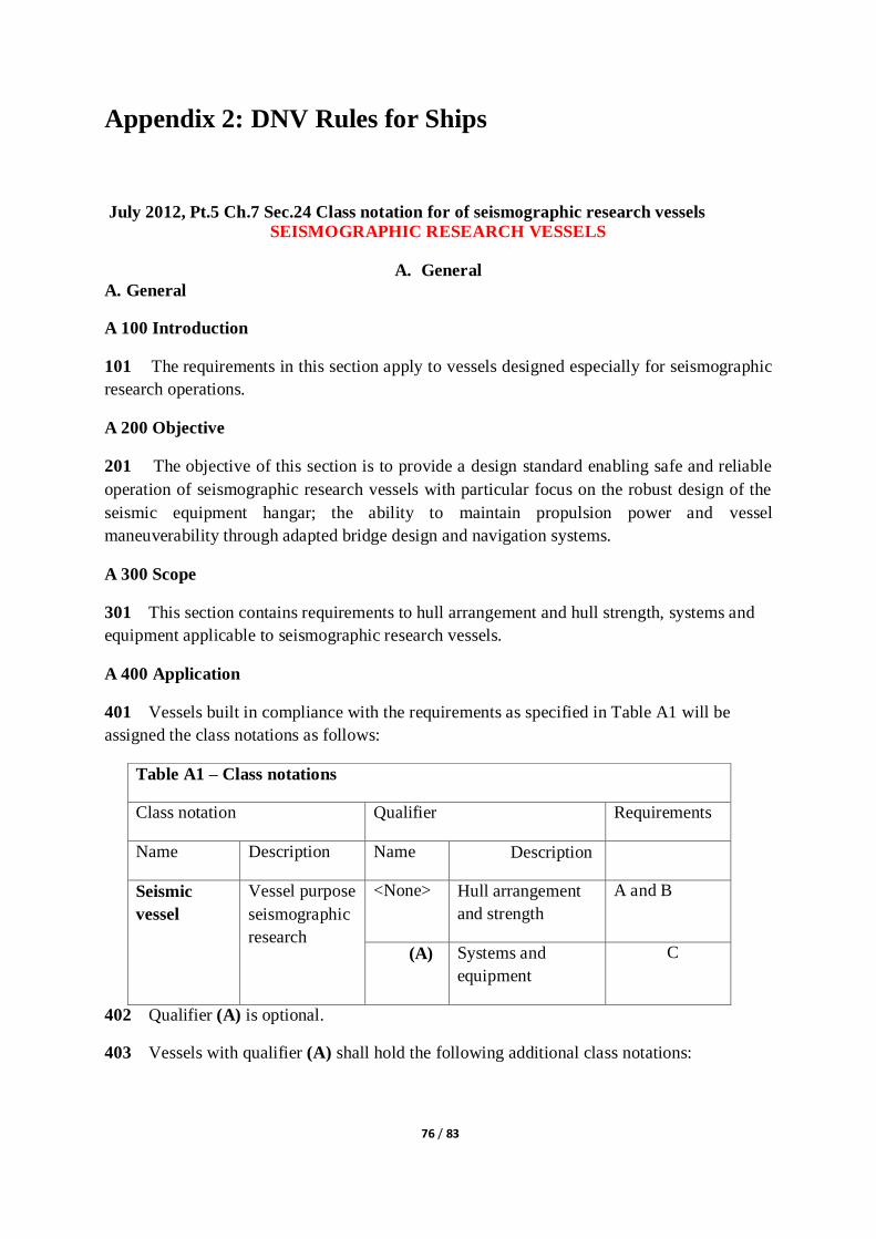
76 / 83

Appendix 2: DNV Rules for Ships

July 2012, Pt.5 Ch.7 Sec.24 Class notation for of seismographic research vessels

SEISMOGRAPHIC RESEARCH VESSELS

A. General

A. General

A 100 Introduction

101 The requirements in this section apply to vessels designed especially for seismographic

research operations.

A 200 Objective

201 The objective of this section is to provide a design standard enabling safe and reliable

operation of seismographic research vessels with particular focus on the robust design of the

seismic equipment hangar; the ability to maintain propulsion power and vessel

maneuverability through adapted bridge design and navigation systems.

A 300 Scope

301 This section contains requirements to hull arrangement and hull strength, systems and

equipment applicable to seismographic research vessels.

A 400 Application

401 Vessels built in compliance with the requirements as specified in Table A1 will be

assigned the class notations as follows:

Table A1 – Class notations

Class notation Qualifier Requirements

Name Description Name Description

Seismic

vessel

Vessel purpose

seismographic

research

<None> Hull arrangement

and strength

A and B

(A) Systems and

equipment

C

402 Qualifier (A) is optional.

403 Vessels with qualifier (A) shall hold the following additional class notations:

77 / 83

— RP (+) or RPS (+), see Pt.6 Ch.2; or DYNPOS-AUTR or DYNPOS-AUTRO, see Pt.6

Ch.7; or

DYNPOS-ER, see Pt.6 Ch.26

— E0 or ECO, see Pt.6 Ch.3

— NAUT- OSV(A), see Pt.6 Ch.20

A 500 Documentation Requirements

501 Documentation shall be submitted as required by Table A2.

Table A2 Document requirements

Object Documentation type Additional description info

Seismic

handling

equipment

C010 – Design criteria Design loads (safe working load,

fleet angles, brake rendering load

and wire breaking load as

relevant). Self-weights of

equipment in operational and in

transit modes.

F1

Z030 Arrangement plan Heavy machinery in hangar and

on deck and equipment for

handling and storage and mooring

at sea.

F1

Z030 Calculation report Hangar: Design loads and racking

calculations covering operational

and transit modes.

F1

Seismic

equipment

supporting

structures

H050 Structural drawing Including foundations. Design

loads, footprint loads and

fastening details.

AP

Work boat

davits

C060 – Mechanical

component

documentation

Including: Safe working load,

heel/trim if applicable and

dynamic factor if above 1.5.

AP

Z160 – Operation manual F1

Z170 – Installation

manual

F1

Z180 – Maintenance

manual

F1

Work boat

davit

winches

C060 – Mechanical

component

documentation

Including: Safe working load,

heel/trim if applicable and

dynamic factor if above 1.5.

AP

Z160 – Operation manual F1

Z170 – Installation

manual

F1

Z180 – Maintenance

manual

F1

78 / 83

Work boat

davits and

winches

supporting

structures

H050 Structural drawing Including foundations. Design

loads, footprint loads and

fastening details.

AP

B. Hull Arrangement and Strength

B 100 Design Loads for Seismic Equipment Hangar

101 Loading conditions and load combinations are to be as specified in the Table B1 for

transit vessel mode (fully loaded deck equipment in stowed condition) and operational mode

(seismographic equipment is deployed).

Table B1 Loading conditions and load combinations on the seismic equipment

hangar

Transit Seismic operation

Load

combination

Vertical Transverse Longitudinal Vertical Transverse

(g0+0.5ay)M X X

g0M X X X

0.67 atM X

0.67 alM X

Equipment

load

X X

Sea pressure X X

Guidance note:

Accelerations are to be according to Pt.3 Ch.1 Sec.4. In no case transverse accelerations

(0.67at) are to be less than 0.5g0.

---e-n-d---of---G-u-i-d-a-n-c-e---n-o-t-e---

102 The total weight M is to include steel weight of the hangar, weight of the deck cargo

and fully loaded equipment. For the operational conditions the weight of the equipment can be

reduced by the weight of deployed cables.

103 Combinations of equipment loads are to include maximum operational loads on

seismographic handling equipment (winches, towing points, etc.) which are assumed to be at

least one line with breaking load and remaining lines with safe working load times the

dynamic factor.

In case of maximum transverse loading, safe working load on towing points times dynamic

factor is to be combined with maximum breaking strength on at least one line in the most

79 / 83

unfavorable position (normally the outermost line). Similar for maximum vertical loading the

breaking load is normally to be applied to the mid-span line and combined with SWL time‘s

dynamic factor for the remaining lines.

If the design specification should include combinations with more than one piece of

equipment with breaking load then this is to be included in the load specification of the

seismic equipment hangar.

104 Breaking load need not to be taken greater than the force causing the winch to render.

105 A design dynamic factor of not less than 1.3 shall be applied to the static SWL of the

seismic handling equipment.

106 For the lowermost deck on semi- enclosed hangars, the design load shall be taken as

the greater value of the Rule sea pressure and specified deck load (when below 2t/m2) in

combination with sea pressure. The sea pressure does not need to exceed 30kN/m2, when it is

used in combination with the deck load. For the remaining decks on semi enclosed hangars,

the design load shall be taken as the greater value of the Rule sea pressure and deck load. For

open weather deck located over 1.7Cw (ref. Pt.3 Ch.1 Sec.4) above the Summer Load

Waterline, the design load shall be taken as the greater value of the Rule sea pressure and

deck load.

107 Allowable stresses:

—Normal stresses: 160 f1 N/mm2

—Shear stresses: 90 f1 N/mm2

B 200Supporting Structures for Seismic Handling Equipment

201 Local structural strength in way of the equipment foundation is to be in compliance

with Pt.3 Ch.3 Sec.5.

202 In case the winch is supported by two deck levels, then local support at one deck level

shall be capable of bearing all vertical loads from the winch.

203 When part of the equipment is acting as structural hull support (i.e. winch frame

providing pillar support for the decks) it is to comply with the strength requirements as for the

main structure with respect to the design loads and Rule acceptance criteria.

204 In cases when equipment is being used as hull structural support this is to be stated in

Memo to Owner (MO) and Appendix to Class Certificate.

B 300Strengthening for Side-By-Side Mooring

80 / 83

301 The SWL for the mooring bollard shall be at least 3 times the minimum breaking load

of the mooring lines according to the vessel‘s equipment letter, or based upon the designer‘s

specification for the minimum breaking load to be used for side-by-side mooring lines.

302 The mooring line specification and restrictions on operation of the mooring bollards are

to be stated in the Appendix to Class Certificate and in a Memo to Owner.

303 The strength of supporting deck structure is to be based on the mooring bollard‘s SWL

times 1.5.

304 Allowable stresses:

—Normal stresses: 160 f1 N/mm2

—Shear stresses: 90 f1 N/mm2

C. Systems and Equipment

C 100 Certification Requirements

101 Components shall be certified as required by Table A3.

Table A3 Certification requirements

Object Certificate type Additional description

Work boats NV-P DNV product

certificate

DNV Standard for Certification

2.21 – Craft

Wide tow equipment

NV-P DNV product

certificate

DNV Standard for Certification

2.22 – Lifting Appliances,

normally as ‗Industrial crane‘ Handling and

towing booms

NV-P DNV product

certificate

Work boat davits NV-P DNV product

certificate

NV-M DNV material

certificate

EN 10204

Work boat winches NV-P DNV product

certificate

NV-M DNV material

certificate

EN 10204

102 For a definition of the certificate types, see Pt.1 Ch.1 Sec.4 B.

C 200Work Boat Davits and winches

201 Where fitted, work boat davits and winches, unless otherwise required by national

authorities are to comply with SOLAS 1974 and the LSA Code, with the following exceptions:

—No requirements to heel or trim unless specified by operator.

—Stored mechanical power not required, however lowering in dead ship condition shall be

possible.

81 / 83

—No requirements to hoisting or lowering speed.

—If estimated dynamic factor exceeds 1.5, shock damper arrangement is required.

202 In addition to strength requirements given in above regulations, fatigue according to a

recognized standard to be considered.

203 Testing at factory and after installation on board shall be performed in line with IMO

MSC. 81(70) part 2.

C 300High pressure air system

301 The piping system shall comply with the requirements in Pt.4 Ch.6. In addition, the

requirements specified in 302 to 311 are to be fulfilled.

302 High pressure pipes shall not be installed in the vicinity of gangways or other spaces

which are in normal use by personnel. If this cannot be avoided, shielding or equivalent

arrangement shall be applied.

Any manifold and pressure relief valve shall be shielded to safeguard any operator. The

pressure relief valves shall be arranged for venting to exhaust or overboard.

Guidance note:

Example of appropriate shielding may be punched steel shields. The shielding may also be

removable in order for accessing de-pressurized equipment.


303 Pipes should be inclined relative to the horizontal. Water pockets in the pipeline shall

be avoided as far as practicable. If this cannot be avoided, means of drainage shall be

arranged.

304 All manifolds and other locations where liquid may accumulate shall be arranged with

possibilities for efficient drainage. Automated drains shall be arranged for air receivers, with

additional possibility for manual operation.

305 Lubricating oil points for the air guns shall not be located in the vicinity of manifolds. If

this cannot be avoided, there shall be arranged automatic shutdown of lubrication pumps

when the high pressure air system is not pressurized.

306 All valves shall be automatically operated in order to prevent adiabatic compression or

water hammer in the system. Alternatively, the system shall always be de-pressurized before

operating any valves.

Guidance note 1:

Opening time of a valve shall be at least 10 seconds.

82 / 83

Controlled pressure adjustment before opening a high pressure valve may, in some cases

serve as an equivalent to automatically operated valves. By adjusting the system pressure to

1:8 of design pressure, the risk of generating high temperatures through adiabatic compression

is negligible.


Guidance note 2:

In cases where automatic operation is not possible to install, each valve shall be permanently

marked with warning against rapid opening.


307 Air intakes for the compressors shall be so located as to minimize the intake of oil or

water contaminated air.

308 Pipes from air compressors with automatic start shall be fitted with a separator or

similar device to prevent condensate and HP piping must be done in a way to prevent

condensate from draining back into compressors.

309 Cylinder banks shall be located in areas which are not in normal use by personnel. The

area shall be arranged for high pressure air to expand in case of an explosion.

Guidance note:

Proper shielding of connected piping and valves may be considered as an equivalent solution

if designated areas cannot be arranged.


310 There shall be at least one burst disc installed at the manifold, and one at the cylinder

bank. The discs shall be directed away from working areas.

311 The piping shall be hydrostatically tested for at least 30 minutes in the presence of a

DNV surveyor after installation on board with the following test pressure:

PH = 1.5 p

PH =test pressure in bar

p =design pressure in bar as defined in Pt.4 Ch.6 Sec.7 A303.

The test pressure need not exceed the design pressure by more than 70 bar.