TECHNOLOGY IN MATHEMATICS CLASSROOMS: A META-ANALYSIS OF THE

*E-mail: [email protected]

Journal of Econometrics 86 (1998) 221—241

Estimation and comparison of multiple change-pointmodels

Siddhartha Chib*John M. Olin School of Business, Washington University, 1 Brookings Drive, Campus Box 1133,

St. Louis, MO 63130, USA

Received 1 January 1997; received in revised form 1 August 1997; accepted 22 September 1997

Abstract

This paper provides a new Bayesian approach for models with multiple change points.The centerpiece of the approach is a formulation of the change-point model in terms ofa latent discrete state variable that indicates the regime from which a particular observa-tion has been drawn. This state variable is specified to evolve according to a discrete-timediscrete-state Markov process with the transition probabilities constrained so that thestate variable can either stay at the current value or jump to the next higher value. Thisparameterization exactly reproduces the change point model. The model is estimated byMarkov chain Monte Carlo methods using an approach that is based on Chib (1996).This methodology is quite valuable since it allows for the fitting of more complex changepoint models than was possible before. Methods for the computation of Bayes factors arealso developed. All the techniques are illustrated using simulated and real datasets. ( 1998 Published by Elsevier Science S.A. All rights reserved.

JEL classification: C1; C4

Keywords: Bayes factors; Change points; Gibbs sampling; Hidden Markov model; Mar-ginal likelihood; Markov mixture model; Markov chain Monte Carlo; Monte Carlo EM

1. Introduction

1.1. Change-point model

This paper is concerned with the problems of estimating and comparingtime-series models that are subject to multiple change points. Suppose

0304-4076/98/$19.00 ( 1998 Published by Elsevier Science S.A. All rights reserved.PII S 0 3 0 4 - 4 0 7 6 ( 9 7 ) 0 0 1 1 5 - 2

½n"My

1, y

2,2,y

nN is a time series such that the density of y

tgiven ½

t~1(with

respect to some p-finite measure) depends on a parameter mt

whose valuechanges at unknown time points ¶

m"Mq

1,2,q

mN and remains constant other-

wise, where q1'1 and q

m(n. Upon setting

mt"G

h1

if t)q1,

h2

if q1(t)q

2,

F F F

hm

if qm~1

(t)qm,

hm`1

if qm(t)n,

where hk3Rd, the problems of inference include the estimation of the parameter

vector H"(h1,2,h

m`1), the detection of the unknown change points

¶m"(q

1,2,q

m), and the comparison of models with different numbers of

change points.This multiple change-point model has generated an enormous literature. One

question concerns the specification of the jump process for the mt. In the

Bayesian context this is equivalent to the joint prior distribution of the qkand

the hk, the parameters of the different ‘regimes’ induced by the change points.

The model is typically specified through a hierarchical specification in which(for every time point t) one first models the probability distribution of achange, given the previous change points; then, the process of the parameters inthe current regime, given the current change points and previous parameters;and finally, the generation of the data, given the parameters and the changepoints.

Chernoff and Zacks (1964) propose a special case of this general model inwhich there is a constant probability of change at each time point (not depen-dent on the history of change points). Then, given that the process has experi-enced changes at the points ¶

k~1"(q

1,2,q

k~1), the parameter vector h

kin the

new regime, conditioned on the parameters Hk~1

of the previous regimes, isassumed to be drawn from some distribution h

kDh

k~1that depends only on h

k~1.

The parameters of this distribution, referred to as hyperparameters, are eitherspecified or estimated from the data. For instance, one may let h

kDH

k~1,

¶k~1

&N(hk~1

, R0), where N denotes the normal distribution and R

0(the

variance matrix) is the hyperparameter of this distribution.Yao (1984) specified the same model for the change points but assumed that

the joint distribution of the parameters MhkN is exchangeable and independent of

the change points. Similar exchangeable models for the parameters have beenstudied by Carlin et al. (1992) in the context of a single change point and byInclan (1993) and Stephens (1994) in the context of multiple change points. Barryand Hartigan (1993) discussed alternative formulations of the change points interms of product partition distributions.

222 S. Chib / Journal of Econometrics 86 (1998) 221–241

One purpose of this paper is to show that it is possible to extend the literatureand fit models in which the change-point probability is not a constant butdepends on the regime. In this case, the probability distribution of the changepoints is characterized not by just one parameter but by a set of parameters (say)P. The precise definition of these parameters is explained in Section 2 below.

Consider the distribution of the data given the parameters. Let ½i"(y

1,2,y

i)

denote the history through time i, and ½i,j"(yi, y

i`1,2,y

j) the history from

time i through j. Then the joint density of the data conditional on (H, ¶m) is

given by

f (½nDH,¶

m)"

m`1<k/1

f (½qk~1`1,qkD½qk~1, h

k, q

k), (1)

where q0"0, q

m`1"n, and f ( ) ) is a generic density or mass function. This is

obtained by applying the law of total probability to the partition induced by ¶m.

A feature of this problem is that the density f (½nDH,P), obtained by marginaliz-

ing f (½nDH,¶

m) over all possible values of Mq

jN with respect to the prior mass

function on ¶m, is generally intractable.

1.2. An existing computational approach

The intractability of f (½nDH, P) has led to some interesting approaches based

on Markov chain Monte Carlo simulation methods. One idea due to Stephens(1994) (see Barry and Hartigan, 1993 for an alternative approach) is to samplethe unknown change points ¶

mand the parameters from the set of full condi-

tional distributions

H, PD½n, ¶

m; q

kD½

n, H, P, ¶

mCk, k)m, (2)

where P denotes (generically) the parameters of the change-point process and

¶mCk

"(q1,2,q

k~1, q

k`1,2,q

m)

is the set of change points excluding the kth. The essential point is that theconditional distribution H, PD½

n, ¶

mis usually simple, whereas each of the

conditional distributions qkD½

n, H, P, ¶

mCkdepends on the two neighboring

change points (qk~1

, qk`1

) and on the data ½qk~1`1,qk`1. Specifically,qkD½

n, H, P, ¶

mCkis given by the mass function

Pr(qk"jD½

n, H, P, ¶

mCk)"Pr(q

k"jD½qk`1

, hk, h

k`1, P, q

k~1, q

k`1)

Jf (½qk~1`1,jD½qk, hk)]f (½j`1, qk`1~1D½

j, h

k`1)]Pr(q

k"jDq

k~1),

for qk~1

(j(qk`1

. The normalizing constant of this mass function is the sum ofthe right-hand side over j.

This approach suffers from two weaknesses. Both are connected to thesimulation of the change points. The first arises from the fact that the change

S. Chib / Journal of Econometrics 86 (1998) 221–241 223

points ¶m

are simulated one at a time from the m full conditional distributionsqkD½

n, H, P, ¶

mCkrather than from the joint distribution

¶mD½

n, H, P.

Sampling the latter distribution directly, say through a Metropolis—Hastingsstep, is not practical because of the difficulty of developing appropriate proposalgenerators for the change points. Liu et al. (1994) in theoretical work and Carterand Kohn (1994), Chib and Greenberg (1995) and Shephard (1994) in empiricalwork have shown that the mixing properties of the MCMC output is consider-ably improved when highly correlated components are grouped togetherand simulated as one block. Conversely, MCMC algorithms that do notexploit such groupings tend to be slow to converge. The second is thecomputational burden in evaluating the joint density functionsf (½qk~1`1,jD½qk, h

k)]f (½j`1,qk`1~1D½

j, h

k`1) for each value of j in the support

qk~1

(j(qk`1

. This calculation must be repeated for each break point leadingto individual density evaluations of the order nm. With a long time series runninginto several hundreds of observations, these calculations are too burdensome tobe practical for even relatively small values of m.

1.3. Outline of paper

The rest of the paper is organized as follows. In Section 2, a new parameteriz-ation of the change point model and an associated MCMC algorithm is suppliedthat eliminates the weaknesses of existing approaches. The MCMC implementa-tion is shown to be straightforward and a simple consequence of the approachdeveloped by Chib (1996) for hidden Markov models. In Section 3 the problemof model comparison is considered and approaches for estimating the likelihoodfunction, the maximum-likelihood estimate, and the Bayes factors for compar-ing change-point models are provided. It is shown that the Bayes factors can bereadily obtained from the method of Chib (1995) in conjunction with theproposed parameterization of the model. Section 4 contains examples of theideas and Section 5 concludes.

2. A new parameterization

We begin this section by providing a new formulation of the change-pointmodel that lends itself to straightforward calculations. This formulation is basedon the introduction of a discrete random variable s

tin each time period, referred

to as the state of the system at time t, that takes values on the integersM1, 2,2,m#1N and indicates the regime from which a particular observationythas been drawn. Specifically, s

t"k indicates that the observation y

tis drawn

from f (ytD½

t~1, h

k).


The variable st

is modeled as a discrete time, discrete-state Markovprocess with the transition probability matrix constrained so that the modelis equivalent to the change-point model. To accomplish this, the transitionprobability matrix specifies that s

tcan either stay at the current value or jump to

the next higher value. This one-step ahead transition probability matrix isrepresented as

P"Ap11

p12

0 2 0

0 p22

p23

2 0

F F F F F

2 F 0 pmm

pm,m`1

0 0 2 0 1 B , (3)

where pij"Pr(s

t"jDs

t~1"i) is the probability of moving to regime j at time

t given that the regime at time t!1 is i. The probability of change thus dependson the current regime, a generalization of both Yao (1984) and Barry andHartigan (1993) (it is easy to make the p

iia function of covariates through

a probit link function, if desired). It is specified that the chain begins in state 1 att"1, implying that the initial probability mass function on the states is(1, 0,2,0), and the terminal state is m#1. Note that there is only one unknownelement in each row of P.

One way to view this parameterization is as a generalized change-point modelin which the jump probabilities p

ii(i)m) are dependent on the regime and the

transitions of the state identify the change points ¶m"(q

1,2,q

m). The kth

change occurs at qk

if sqk"k and sqk`1"k#1. Note that this reparameteriz-

ation automatically enforces the order constraints on the break points. Anotherway to view this parameterization is as a hidden Markov model (HMM) (Chib,1996) in which the transition probabilities of the hidden state variable s

tare

restricted in the manner described above. This view of the model forms the basisof our computational MCMC scheme.

2.1. Markov chain Monte Carlo scheme

Suppose that we have specified a prior density n(H, P) on the parameters andthat data ½

nis available. In the Bayesian context, interest centers on the

posterior density n(H, PD½n)Jn(H, P) f (½

nDH, P). Note that we use the notation

n to denote prior and posterior density functions of (H, P). This posteriordensity is most fruitfully summarized by Markov chain Monte Carlo methodsafter the parameter space is augmented to include the unobserved statesSn"(s

1,2,s

n) (see Chib and Greenberg, 1996 for a convenient summary of these

methods). In other words, we apply our Monte Carlo sampling scheme to theposterior density n(S

n, H, PD½

n).


The general sampling method works recursively. First, the states Sn

aresimulated conditioned on the data ½

nand the other parameters (where s

nis set

equal to m#1), and second, the parameters are simulated conditioned on thedata and S

n. Specifically, the MCMC algorithm is implemented by simulating

the following full conditional distributions:

1. H, PD½n, S

n, and

2. SnD½

n, H, P,

where the most recent values of the conditioning variables are used in allsimulations. Note that the first distribution is the product of PDS

nand

HD½n, S

n, P. The latter distribution is model specific and is therefore discussed

only in the context of the examples below.

2.2. Simulation of MstN

Consider now the question of sampling Snfrom the distribution S

nD½

n, H, P,

which amounts to the simulation of ¶m

from the joint distribution ¶mD½

n, H, P.

As mentioned earlier, sampling the change points from the latter distribution isdifficult, if not impossible, however, the simulation of the states from the formerdistribution is relatively straightforward and requires just two passes throughthe data, regardless of the number of break points. Because the MCMC sampleson the states are obtained by sampling the joint distribution, significant im-provements in the overall mixing properties of the output (relative to theone-at-a time sampler) can be expected. In addition, this algorithm producesconsiderable time savings, requiring merely order n conditional density evalu-ations of y

t.

The algorithm for sampling the states follows from Chib (1996), where theunrestricted Markov mixture model is analyzed by MCMC methods. Theobjective is to draw a sequence of values of s

t3M1, 2,2,m#1N from the mass

function p(SnD½

n, H, P). Henceforth, the notation p( ) ) is used whenever one is

dealing with a discrete mass function. Let

St"(s

1,2,s

t); St`1"(s

t`1,2,s

n),

denote the state history up to time t and the future from t#1 to n, respectively,with a similar convention for ½

tand ½t`1, and write the joint density in reverse

time order as

p(sn~1

D½n, s

n, H, P)]2]p(s

tD½

n, St`1, H, P)]2]p(s

1D½

n, S2, H, P).

(4)

We write the joint density in this form because only then can each of themass functions be derived and sampled. The process is completed by sampling,


in turn,

f sn~1

from p(sn~1

D½n, s

n"m#1, H, P),

f sn~2

from p(sn~2

D½n, Sn~1, H, P),

f Ff s

1from p(s

1D½

n, S2, H, P).

The last of these distributions is degenerate at s1"1. Thus, to implement this

sampling it is sufficient to consider the sampling of stfrom p(s

tD½

n, St`1, H, P).

Chib (1996) showed that

p(stD½

n, St`1, H, P)Jp(s

tD½

t, H, P)p(s

t`1Dst, P), (5)

where the normalizing constant is easily obtained since sttakes on only two

values, conditioned on the value taken by st`1

. There are two ingredients in thisexpression — the quantity p(s

tD½

t, H, P) and p(s

t`1Dst, H, P), which is just the

transition probability from the Markov chain. To obtain the mass functionp(s

tD½

t, H, P), t"1,2,2,n, a recursive calculation is required. Starting with

t"1, the mass function p(st~1

D½t~1

, H, P) is transformed into p(stD½

t, H, P)

which in turn is transformed into p(st`1

D½t`1

, H, P), and so on. The details areas follows. Suppose p(s

t~1"lD½

t~1, H, P) is available. Then, the update to the

required distribution is given by

p(st"kD½

t, H, P)"

p(st"kD½

t~1,H, P)]f (y

tD½

t~1, h

k)

+kl/k~1

p(st"lD½

t~1,H,P)]f (y

tD½

t~1,h

l),

where

p(st"kD½

t~1, H, P)"

k+

l/k~1

plk]p(s

t~1"lD½

t~1, H, P), (6)

for k"1, 2,2, m#1, and plk

is the Markov transition probability in Eq. (3).These calculations are initialized at t"1 by setting p(s

1D½

0, h) to be the mass

distribution that is concentrated at 1. With these mass functions at hand, thestates are simulated from time n (setting s

nequal to m#1) and working

backwards according to the scheme described in Eq. (5).It can be seen that the sample output of the states can be used to determine the

distribution of the change points. Alternatively, posterior information aboutchange points can be based on the distribution

Pr(stD½

n)"Pp(s

t"kD½

t~1, H, P)n(H, PD½

n)d(H, P).

This implies that a Monte Carlo estimate of Pr(stD½

n) can be found by taking an

average of p(st"kD½

t~1, H, P) over the MCMC iterations. By the Rao—Black-

well theorem, this estimate of Pr(stD½

n) is more efficient than one based on the

empirical distribution of the simulated states.


2.3. Simulation of P

The revision of the non-zero elements pii

in the matrix P given the data andthe value of S

nis straightforward since the full conditional distribution

PD½n, S

n, H is independent of (½

n, H), given S

n. Thus, the elements p

iiof P may

be simulated from PDSnwithout regard to the sampling model for the data y

t(see

Albert and Chib, 1993).Suppose that the prior distribution of p

ii, independently of p

jj, jOi, is Beta,

i.e.,

pii&Beta(a,b)

with density

n(piiDa,b)"

C (a#b)

C (a)C (b)pa~1ii

(1!pii)b~1,

where a< b. The joint density of P is, therefore, given by

n(P)"cm<i/1

p(a~1)ii

(1!pii)(b~1)

where c"M(C(a#b))/(C(a)C(b))Nm. The parameters a and b may be specified sothat they agree with the prior beliefs about the mean duration of each regime.Because the prior mean of p

iiis equal to pN "a/(a#b), the prior density of the

duration d in each regime is approximately n(d)"pN d~1(1!pN ) with prior meanduration of (a#b)/b. Let n

iidenote the number of one-step transitions from

state i to state i in the sequence Sn. Then multiplying the prior by the likelihood

function of PDSn

yields

piiDS

n&Beta(a#n

ii, b#1), i"1,2,m, (7)

since ni,i`1

"1. The probability pii

(1)i)m) can now be simulated fromEq. (7) by letting

pii"

x1

+2j/1

xj

, x1&Gamma(a#n

ii, 1); x

2&Gamma(b#1, 1)

This completes the simulation of Snand the non-zero elements of P.

3. Bayes factor calculation

In this section we consider the comparison of alternative change-point models(e.g., a model with one change point vs. one with more than one change point).The Bayesian framework is particularly attractive in this context because these


models are non-nested. In such settings, the marginal likelihood of the respectivemodels, and Bayes factors (ratios of marginal likelihoods), are the preferredmeans for comparing models (Kass and Raftery, 1995; Berger and Perrichi,1996).

The computation of the marginal likelihood using the posterior simulationoutput has been an area of much current activity. A method developed by Chib(1995) is particularly simple to implement. The key point is that the marginallikelihood of model M

r

m(½nDM

r)"P f (½

nDM

r, H, P)n(H, P)DM

r) dt

may be re-expressed as

m(½nDM

r)"

f (½nDM

r, H*, P*)n(H*, P*DM

r)

n(H*, P*D½n, M

r)

, (8)

where (H*, P*) is any point in the parameter space. Note that, for convenience,the notation does not reflect the fact that the size of the parameter space, and theparameters, are model dependent. The latter expression, which has been calledthe basic marginal likelihood identity, follows from Bayes theorem. This expres-sion requires the value of the likelihood function f (½

nDM

r, t*) at the point

t*"(H*, P*) along with the prior and posterior ordinates at the same point.These quantities are readily obtained from the MCMC approach discussedabove. The choice of the point t* is in theory completely irrelevant but inpractice it is best to choose a high posterior density point such as the maximum-likelihood estimate or the posterior mean. Given estimates of the marginallikelihood for two models M

rand M

s, the Bayes factor of r vs. s is defined as

Brs"

m(½nDM

r)

m(½nDM

s).

Large values of Brs

indicate that the data support Mrover M

s(Jeffreys, 1961).

In the rest of the discussion we explain how each of the quantities required forthe marginal likelihood calculation is obtained. The model index M is sup-pressed for convenience.

3.1. Likelihood function at t*"(H*, P*)

A simple method for computing the likelihood function is available from theproposed parameterization of the change-point model. It is based on thedecomposition

ln f (½nDt*)"

n+t/1

ln f (ytD½

t~1, t*),


where

f (ytD½

t~1, t*)"

m+k/1

f (ytD½

t~1, t*, s

t"k)p(s

t"kD½

t~1, t*) (9)

is the one-step ahead prediction density. The quantity f (ytD½

t~1, t*, s

t"k) is

the conditional density of ytgiven the regime s

t"k whereas p(s

t"kD½

t~1, t*) is

the mass in Eq. (6). The one-step ahead density (and, consequently, the jointdensity of the data) is thus easily obtained. It should be noted that the likelihoodfunction is required at the selected point t* for the computation of the marginallikelihood. It is not required for the MCMC simulation.

3.2. Estimation by simulation

A Monte Carlo version of the EM algorithm can be used to find the maximumlikelihood estimate of the parameters (H, P). This estimate can be used as thepoint t* in the calculation of the marginal likelihood.

Note that the EM algorithm entails the following steps: First, the computa-tion of the function

Q(t, t(i))"PSn

ln ( f (½n, S

nDt))p(S

nD½

n, t(i)) dS

n, (10)

which requires integrating Sn

out from the complete data joint densityf (½

n, S

nDt) with respect to the current distribution of S

ngiven ½

nand the current

parameter estimate t(i). The second step is the maximization of this function toobtain the revised value t(i`1).

Due to the intractability of the integral above, the first step is implemented bysimulation. Because the integration is with respect to the joint distribution

p(SnD½

n, t(i)),p(s

1, s

2,2,s

nD½

n, t(i)), (11)

the Q function may be calculated as follows (see also Wei and Tanner, 1990). LetSn,j

(j)N) denote the N draws of Snfrom p(S

nD½

n, t(i)) and let

QK (t)"N~1N+j/1

lnM f (½n, S

n,jDt)N"N~1

N+j/1

Mln f (½nDS

n,j,H)#ln f (S

n,jDP)N.

(12)

The M-step is implemented by maximizing the QK function over t. This two-stepprocess is iterated until the values t(i) stabilize (N is usually set small at the startof the iterations and large as the maximizer is approached). The quantity thusobtained is the (approximate) maximum-likelihood estimate.

Each of these steps is quite easy. Estimating the Q function requires draws onSn, and these are obtained by the method discussed in Section 2.1. In the M-step,


the maximization is usually straightforward and separates conveniently into oneinvolving H in the sampling model and one involving P in the jump process. Thelatter estimates are

pLii"

+Nj/1

nii,j

+Nj/1

(nii,j

#1), i"1,2,m, (13)

where nii,j

is equal to the number of transitions from state i to state i in the vectorSn,j

.

3.3. Marginal likelihood

The estimate of the marginal likelihood is completed by computing the valueof the posterior ordinate n(t*D½

n) at t*. By definition of the posterior density

n(H*, P*D½n)"n(H*D½

n)n(P*D½

n, H*),

where

n(H*D½n)"Pn(H*D½

n, S

n)p(S

nD½

n) dS

n(14)

and

n(P*D½n, H*)"Pn(P*DS

n)p(S

nD½

n, H*) dS

n, (15)

since n(P*D½n, H*, S

n)"n(P*DS

n). The first of these ordinates may be estimated

as

nL (H*D½n)"G~1

G+g/1

n(H*D½n, S

n,g),

using the G draws on Sn

from the run of the Markov chain Monte Carloalgorithm. The value n(H*D½

n, S

n,g) may be stored at the completion of each

cycle of the simulation algorithm.The calculation of the second ordinate in Eq. (15) requires an additional

simulation MSn,j

NGj/1

of Snfrom p(S

nD½

n, H*). These draws are readily obtained by

appending a pair of additional calls to the simulation of Sn

conditioned on(½

n, H*, P) and P conditioned on (½

n, H*, S

n) within each cycle of the MCMC

algorithm. Because the ordinate n(P*DSn) is a product of Beta densities from the

first m rows of P, the estimate of the reduced conditional ordinate in Eq. (15) is

nL (P*D½n,H*)"G~1

G+j/1

m<i/1

n(piiDS

n,j)

"G~1G+j/1

m<i/1GC (a#b#n

ii,j#1)

C (a#nii,j

)C (b#1)Hp(a`nii,j~1)ii

(1!pii)(b`1~1).


The log of the marginal likelihood from Eq. (8) is now given by

lnmL (½n)"ln f (½

nDt*)#lnn(H*)#lnn(P*)

!ln nL (H*D½n)!ln nL (P*D½

n,H*). (16)

The calculation of Eq. (16) is illustrated in the examples.

4. Examples

4.1. Binary data with change point

Consider first a sequence of binary observations MytN, where y

t3M0,1N, and

suppose that yt&Bernoulli(m

t), where the probability m

tis subject to change at

unknown time points. This is a canonical but non-trivial problem involvingchange points. To illustrate the ideas discussed above, y

tis simulated from the

process

mt"G

h1, t)50,

h2, 50(t)100,

h3, 100(t)150,

where h1"0.5, h

2"0.75 and h

3"0.25. The data is reproduced (in cumulative

sum form) in Fig. 1. To keep the discussion simple, it is assumed that hk(k)3)

is independent of any covariates. Note that the break at t"50 is not clearlydistinguishable in the graph.

One important inferential question is the estimation of the jump probabilitymatrix

P"Ap11

p12

0

0 p22

p23

0 0 1 Band the change points Mq

1,q2N. A second question is the comparison of models

with a single change point (M1), two change points (M

2), and three change

points (M3). Note that M

1contains the parameters (h

1, h

2, p

11), whereas

M2

and M3

contain the parameters (h1, h

2, h

3, p

11, p

22) and (h

1, h

2,

h3, h

4, p

11, p

22, p

33), respectively.

For the prior distributions, assume exchangeability within each model and let

hkDM

r&Beta(2,2), k)r#1,

piiDM

r&Beta(8,0.1), i)r.


Fig. 1. Binary 0—1 data ytin example 4.1.

The prior on pii

reflects the prior beliefs that in model Mr, the expected duration

of each regime is approximately 80 periods. One could argue that this assump-tion is not reasonable for models M

2or M

3and a prior with shorter expected

duration for these models should be specified (e.g., by letting the first parameterof the Beta distribution be 6 instead of 8). As one would expect, such a priorchanges the marginal likelihood but, in this example, does not alter the rankingsof the models that is reported below. In general, therefore, the key question iswhether the conclusions change (not just whether the Bayes factors change) asthe prior is perturbed by a reasonable amount. This must be ascertained ona case by case basis.

Under these prior distributions, MhkN in model M

r, given the complete condi-

tioning set, are independent with density

n(hkD½

n, S

n, P)"Beta(h

kD2#º

k, 2#N

k!º

k), k)r#1, (17)

where Nk"+n

t/1I(s

t"k) is the number of observations ascribed to regime k

and ºk"+n

t/1I(s

t"k)y

tis the sum of the y

tin regime k. This corresponds to

the familiar Bayesian update for a Bernoulli probability with a single regime k.The MCMC simulation algorithm is completed by simulating Mh

kN from Eq. (17)

and Sn

and P as described in Sections 2.2 and 2.3. The MCMC sampling


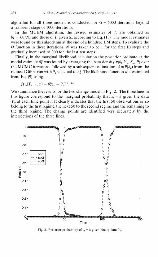
Fig. 2. Posterior probability of st"k given binary data ½

n.

algorithm for all three models is conducted for G"6000 iterations beyonda transient stage of 1000 iterations.

In the MCEM algorithm, the revised estimates of hk

are obtained ashKk"º

k/N

kand those of P given S

naccording to Eq. (13). The modal estimates

were found by this algorithm at the end of a hundred EM steps. To evaluate theQ function in these iterations, N was taken to be 1 for the first 10 steps andgradually increased to 300 for the last ten steps.

Finally, in the marginal likelihood calculation the posterior ordinate at themodal estimate h*

kwas found by averaging the beta density n(h

kD½

n, S

n, P) over

the MCMC iterations, followed by a subsequent estimation of n(PDSn) from the

reduced Gibbs run with hkset equal to h*

k. The likelihood function was estimated

from Eq. (9) using

f (ytD½

t~1, s

t)"hyt

st(1!h

st)(1~yt).

We summarize the results for the two change model in Fig. 2. The three lines inthis figure correspond to the marginal probability that s

t"k given the data

½nat each time point t. It clearly indicates that the first 50 observations or so

belong to the first regime, the next 50 to the second regime and the remaining tothe third regime. The change points are identified very accurately by theintersections of the three lines.


Table 1Maximized log-likelihood and log marginal likelihood for binary data

M1

(One change point) M2

(Two change points) M3

(Three change points)

ln f (½nDt*) !97.548 !92.912 !92.326

lnm(½n) !103.665 !101.872 !102.402

We report in Table 1 the evidence in the data for each of the three models.The results imply that the Bayes factor B

21is approximately six, while B

23is

approximately 1.7. These Bayes factor provide (moderate) evidence in favor ofthe two change-point model in relation to the two competing models.

4.2. Poisson data with change point

As another illustration of the methods in the paper consider the muchanalyzed data on the number of coal-mining disasters by year in Britain over theperiod 1851—1962 (Jarrett, 1979). Let the count y

tin year t be modeled via

a hierarchical Poisson model

f (ytDm

t)"myt

te~mt/y

t! (t)112)

and consider determining the evidence in favor of three models M1!M

3.

Under M1, the no change point case, m

t"j, j&Gamma(2,1). Under M

2,m

tis

subject to a single break:

mt"G

j1

for t)q1,

j2

for q1#1)t)112

with

j1, j

2&Gamma(2,1).

Finally, under model M3, m

tis subject to two breaks with

j1, j

2, j

3&Gamma(3,1).

The data on ytis reproduced in Fig. 3. In this context it is of interest to fit all

three models and to determine the Bayes factor B12

for 1 vs. 2, B13

for 1 vs. 3 andB23

for 2 vs. 3.Carlin et al. (1992), in their analysis of these data, use a hierarchical Poisson

Bayesian model and fit the one change-point model and find that the posteriormass function on q

1is concentrated on the observations 36—46 with a mode at

y41

. The three largest spikes are at t"39, 40, and 41, corresponding to a changesometime between 1889 and 1892. These results are also easily reproduced from


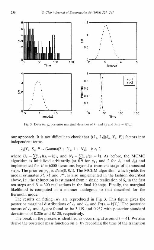
Fig. 3. Data on yt, posterior marginal densities of j

1and j

2and Pr(s

t"kD½

n).

our approach. It is not difficult to check that M(j1, j

2)D(S

n, ½

n, P)N factors into

independent terms

jkD½

n, S

n, P&Gamma(2#º

k, 1#N

k), k)2,

where ºk"+n

t/1I(s

t"k)y

tand N

k"+n

t/1I(s

t"k). As before, the MCMC

algorithm is initialized arbitrarily (at 0.9 for p11

and 2 for j1

and j2) and

implemented for G"6000 iterations beyond a transient stage of a thousandsteps. The prior on p

11is Beta(8, 0.1). The MCEM algorithm, which yields the

modal estimates j*1, j*

2and P*, is also implemented in the fashion described

above, i.e., the Q function is estimated from a single realization of Snin the first

ten steps and N"300 realizations in the final 10 steps. Finally, the marginallikelihood is computed in a manner analogous to that described for theBernoulli model.

The results on fitting M2

are reproduced in Fig. 3. This figure gives theposterior marginal distributions of j

1and j

2and Pr(s

t"kD½

n). The posterior

means of j1

and j2

are found to be 3.119 and 0.957 with posterior standarddeviations of 0.286 and 0.120, respectively.

The break in the process is identified as occurring at around t"41. We alsoderive the posterior mass function on q

1by recording the time of the transition


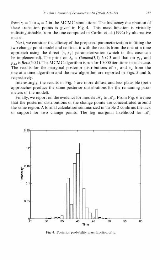
Fig. 4. Posterior probability mass function of q1.

from st"1 to s

t"2 in the MCMC simulations. The frequency distribution of

these transition points is given in Fig. 4. This mass function is virtuallyindistinguishable from the one computed in Carlin et al. (1992) by alternativemeans.

Next, we consider the efficacy of the proposed parameterization in fitting thetwo change-point model and contrast it with the results from the one-at-a timeapproach using the direct Mq

1,q2N parameterization (which in this case can

be implemented). The prior on jk

is Gamma(3,1), k)3 and that on p11

andp22

is Beta(5,0.1). The MCMC algorithm is run for 10,000 iterations in each case.The results for the marginal posterior distributions of q

1and q

2from the

one-at-a time algorithm and the new algorithm are reported in Figs. 5 and 6,respectively.

Interestingly, the results in Fig. 5 are more diffuse and less plausible (bothapproaches produce the same posterior distributions for the remaining para-meters of the model).

Finally, we report on the evidence for models M1

to M3. From Fig. 6 we see

that the posterior distributions of the change points are concentrated aroundthe same region. A formal calculation summarized in Table 2 confirms the lackof support for two change points. The log marginal likelihood for M

1


Fig. 5. Posterior probability function of q1

(top panel) and q2: One-at-a time algorithm.

Fig. 6. Posterior probability function of q1

(top panel) and q2: New algorithm.


Table 2Maximized log-likelihood and log marginal likelihood for coal mining disaster data

M1

(No change point) M2

(One change points) M3

(Two change points)

ln f (½nDt*) !203.858 !172.181 !171.450

lnm(½n) !206.365 !179.684 !180.836

is !206.365 and that of M2

is !172.181, implying decisive evidence in favorof M

2.

The log marginal likelihood of the two change-point model M3

is !180.836,slightly lower than that of M

2. Thus, we are able to conclude that these data do

not support a second change point.

5. Concluding remarks

This paper has proposed a new approach for the analysis of multiplechange-point models. The centerpiece of this approach is a formulation of thechange-point model in terms of an unobserved discrete state variable thatindicates the regime from which a particular observation has been drawn. Thisstate variable is specified to evolve according to a discrete-time, discrete-stateMarkov process with the transition probabilities constrained so that the statevariable can either stay at the current value or jump to the next higher value.This parameterization exactly reproduces the change-point model. In addition,it was shown that the MCMC simulation of this model is straightforward andimproves on existing approaches in terms of computing time and speed ofconvergence.

The paper also provides a means for comparing alternative change-point models through the calculation of Bayes factors. This calculationwhich was hitherto not possible, in general, due to the intractability of thelikelihood function is based on the computation of the marginal likeli-hood of each competing model from the output of the MCMC simulation.These calculations were illustrated in the context of models for binary andcount data.

It is important to mention that the approach proposed here should proveuseful in the development of new approaches for the classical analysis of thechange-point model. Besides providing a simple approach for the computationof the likelihood function and maximum-likelihood estimates, it should allowfor the construction of new tests due to the connection with hidden Markovmodels that is developed in this paper.


Finally, the approach leads to a new analysis for the class of epidemicchange-point models. In a version of this model considered by Yao (1993), anepidemic state is followed by a return to a normal state. This model becomesa special case of the above framework if one restricts the state variable to takethree values such that the parameter values in the first and last state (corres-ponding to the normal state) are identical. The MCMC analysis of the modelthen proceeds with little modification.

Acknowledgements

The comments of the editor, associate editor and two annonymous refereesare gratefully acknowledged.

References

Albert, J., Chib, S., 1993. Bayes inference via Gibbs Sampling of autoregressive time seriessubject to Markov mean and variance shifts. Journal of Business and Economic Statistics 11,1—15.

Barry, D., Hartigan, J., 1993. A Bayesian analysis for change point problems. Journal of theAmerican Statistical Association 88, 309—319.

Berger, J., Pericchi, L., 1993. The intrinsic Bayes factor for model selection and prediction. Journal ofthe American Statistical Association 91, 109—122.

Carlin, B., Gelfand, A., Smith, A.F.M., 1992. Hierarchical Bayesian analysis of change-pointproblems. Applied Statistics 41, 389—405.

Carter, C.K., Kohn, R., 1994. On Gibbs Sampling for state space models. Biometrika 81,541—553.

Chernoff, H., Zacks, S., 1964. Estimating the current mean of a Normal distribution which is subjectto changes in time. Annals of Mathematical Statistics 35, 999—1018.

Chib, S., 1995. Marginal likelihood from the Gibbs output. Journal of the American StatisticalAssociation 90, 1313—1321.

Chib, S., 1996. Calculating posterior distributions and modal estimates in Markov mixture models.Journal of Econometrics 75, 79—98.

Chib, S., Greenberg, E., 1995. Hierarchical analysis of SUR models with extensions to correlatedserial errors and time-varying parameter models. Journal of Econometrics 68, 339—360.

Chib, S., Greenberg, E., 1996. Markov Chain Monte Carlo simulation methods in econometrics.Econometric Theory 12, 409—431.

Inclan, C., 1993. Detection of multiple changes of variance using posterior odds. Journal of Businessand Economic Statistics 11, 289—300.

Jarrett, R.G., 1979. A note on the interval between coal mining disasters. Biometrika 66, 191—193.Jeffreys, H., 1961. Theory of Probability. Oxford University Press, Oxford.Kass, R., Raftery, A., 1995. Bayes factors. Journal of the American Statistical Association 90,

773—795.Liu, J.S., Wong, W.H., Kong, A., 1994. Covariance structure of the Gibbs Sampler with appli-

cations to the comparisons of estimators and data augmentation schemes. Biometrika 81,27—40.

Shephard, N., 1994. Partial non-Gaussian state space. Biometrika 81, 115—131.


Stephens, D.A., 1994. Bayesian retrospective multiple-changepoint identification. Applied Statistics43, 159—178.

Wei, G.C.G., Tanner, M.A., 1990. A Monte Carlo implementation of the EM Algorithm and thePoor Man’s data augmentation algorithm. Journal of the American Statistical Association 85,699—704.

Yao, Y.C., 1984. Estimation of a noisy discrete-time step function: Bayes and Empirical Bayesapproaches. Annals of Statistics 12, 1434—1447.

Yao, Q., 1993. Tests for change-points with epidemic alternatives. Biometrika 80, 179—191.


TECHNOLOGY IN MATHEMATICS CLASSROOMS: A META-ANALYSIS OF THE

Documents