Techniques of the Average Case Analysis of Algorithms · The suffix tree and the compact sujJix tree are similar to the hie and PATRICIA tric, but differ in the structure ofthe words

Purdue UniversityPurdue e-Pubs

Computer Science Technical Reports Department of Computer Science

1996

Techniques of the Average Case Analysis ofAlgorithmsWojciech SzpankowskiPurdue University, [email protected]

Report Number:96-064

This document has been made available through Purdue e-Pubs, a service of the Purdue University Libraries. Please contact [email protected] foradditional information.

Szpankowski, Wojciech, "Techniques of the Average Case Analysis of Algorithms" (1996). Computer Science Technical Reports. Paper1318.http://docs.lib.purdue.edu/cstech/1318

TECHNIQUES OF THE AVERAGECASE ANALYSIS OF ALGORITHMS

Wojciech Szpankowski

Department of Computer SciencePurdue University

West Lafayette, IN 47907

CSD-TR 96-064October 1996

TECHNIQUES OF THE AVERAGE CASE ANALYSIS OF ALGORITHMS

Wojciech Szpankowski*Department of Computer Science

Purdue UniversityW. Lafayette, IN 47907

U.S.A.

Abstract

This is an extended version of a book chapter that I wrote for the Handbook on Al­gorithms and Theon) of Computation (Ed. M. Atallah) in which some probabilistic andanalytical techniques of the average case analysis of algorithms are reviewed. By analyticaltechniques we mean those in which complex analysis plays a primary role. We choose onefacet of the theory of algorithms, namely that of algorithms and data structures on words(strings) and present a brief exposition on certain analytical and probabilistic methods thathave become popular in such an endeavor. Our choice of the area stems from the fact thatthere has been a resurgence of interest in string algorithms due to several novel applica~

tions, most notably in computational molecular biology and data compression. Our choiceof methods covered here is aimed at closing a gap between analytical and probabilistic meth­ods. We discuss such probabilistic methods as: the sieve method, first and second momentmethods, subadditive ergodic theorem, techniques of information theory (e.g., entropy andits applications), and large deviations (i.e., Chernoff's bound) and Azuma's type inequal­ity. Finally, on the analytical side, we survey here certain class of recurrences, complexasymptotics (i.e., Rice's formula, singularity analysis, etc." the Mellin transform and itsapplications, and poissonization and depoissonlzation.

"This research was supported in part by NSF Grants NCR-9206315, NCR-9415491, and CCR-9201078,and in part by NATO Collaborative Grant CGR.950060.

1

Contents

1 Introduction

2 Data Structures and Algorithms on Words2.1 Digital Trees .2.2 String Editing Problem .2.3 Shortest Common Superstring.

3 Probabilistic Models3.1 Probabilistic Models of Strings _ _ .3.2 Quick Review from Probability: Types of Stochastic Convergence.3.3 Review from Complex Analysis .

4 Probabilistic Techniques4.1 Sieve Method and Its Variations .4.2 Inequalities: First and Second Moment Methods4.3 Subadditive Ergodic Theorem .4.4 Entropy and Its Applications .4.5 Central Limit and Large Deviations Results

5 Analytical Techniques5.1 Recurrences and Functional Equations5.2 Complex Asymptotics .5.3 Mellin Transform and Asymptotics

6 References

2

3

4578

10101114

151519232629

34344145

52

1 Introduction

An algorithm is a finite set of instructions for a treatment of data to meet some desired

objectives. The most obvious reason for analysing algorithms and data structures (associ­

ated with them) is to discover their characteristics in order to evaluate their suitability for

various applications or to compare them with other algorithms for the same application.

Needless to say, we are interested in efficient algorithms in order to use efficiently scarce

resources such as computer space and time.

Most often algorithm designs are finalized to the optimization of the asymptotic worst

case performance, as popularized by Aho, Hopcroft and Ullman [2J. Insightful, elegant

and generally useful constructions have been set up in this endeavor. Along these lines,

however, the design of an algorithm is usually targeted at coping efficiently with unrealistic,

even pathological inputs and the possibility is neglected that a simpler algorithm that works

fast 'lon average" might perform just as well, or even better in practice. This alternative

solution, called also a probabilistic approach, became an important issue two decades ago

when it became clear that the prospects for showing the existence of polynomial time

algorithms for NP-hard problems, were very dim. This fact, and apparently high success

rate of heuristic approaches to solving certain difficult problems, led Richard Karp [56J to

undertake a more serious investigation of probabilistic approximation algorithms. (But, one

must realize that there are problems which are also hard "on average" as shown by Levin

[67J.) In the last decade we have witnessed an increasing interest in the probabilistic, also

called average case analysis and design of algorithms, possibly due to the high success rate

of randomized algorithms for computational geometry, scientific visualization, molecular

biology, etc. (e.g., see (14, 42, 75, 97]).

The average case analysis of algorithms can be roughly divided into categories, namely:

analytical (also called precise) and probabilistic analysis of algorithms. The former was

popularized by Knuth's monumental three volumes The Art of Computer Programming

[63, 64, 65J whose prime goal was to accurately predict the performance characteristics of an

algorithm. Such an analysis more than often sheds light on properties of computer programs

and provides useful insights of combinatorial behaviors of such programs. Probabilistic

methods were introduced by Erdos and Renyi and popularized by Erdos and Spencer in

their book [23] (ef. also [5]). In general, nicely structured problems arc amiable to an

analytical approach that usually gives much more precise information about the algorithm

under consideration. On the other hand, structurally complex algorithms are more likely

to be first solved by a probabilistic tool that later could be further enhanced by a more

3

precise analytical approach. The average case analysis of algorithms, as a discipline, uses

a number of branches of mathematics: combinatorics, probability theory, graph theory,

real and complex analysis, and occasionally algebra, geometry, number theory, operations

research, and so forth.

In this chapter, we choose one facet of the theory of algorithms, namely that of algo­

rithms and data structures on words (strings) and present a brief exposition on certain

analytical and probabilistic methods that have become popular in such an endouver. Our

choice of the area stems from a fact that there has been a resurgence of interest in string al­

gorithms due to several novel applications, most notably in computational molecular biology

and data compression. Our choice of methods covered here is aimed at closing a gap between

analytical and probabilistic methods. There are excellent books on analytical methods (d.

Knuth's three volumes [63, 64, 651, Sedgewick and Flajolet [84]) and probabilistic methods

(cf. Alon and Spencer [5], Coffman and Lueker [17], and Motwani and Raghavan [75]), how­

ever, remarkably very few books have been dedicated to both analytical and probabilistic

analysis of algorithms (with possible exceptions of Hofri [45] and Mahmoud [73]). Finally,

before we launch our journey through probabilistic and analytical methods, we should add

that in recent years several useful surveys on analysis of algorithms have been published.

We mentioned here: Karp [57], Vitter and Flajolet [961, and Flajolet [28].

This chapter is organized as follows: In the next section we describe some algorithms

and data structures on words (e.g., digital trees, suffix trees, edit distance, Lempel-Ziv data

compression algorithm, etc.) that we use throughout to illustrate our ideas and methods

of analysis. Then, we present probabilistic models for algorithms and data structures on

words together with a short review from probability and complex analysis. Section 4 is

devoted to probabilistic methods and we discuss the sieve method, first and second moment

methods, subadditive ergodic theorem, techniques of information theory (e.g., entropy and

its applications), and large deviations (i.e., Chernoff's bound) and Azuma's type inequal­

ity. Finally, in the last section we concentrate on analytical techniques that we define as

such in which complex analysis plays an important role. We plan to touch here analytical

techniques for recurrences and asymptotics (i.e., Rice's formula, singularity analysis, etc.),

Mellin transform and its applications, and poissonization and depoissonization.

2 Data Structures and Algorithms on Words

As mentioned above, in this survey we choose one facet of the theory of algorithms, namely

that of data structures and algorithms on words (strings) to illustrate several probabilistic

4

and analytical techniques of the analysis of algorithms. In this section, we briefly recall

to the reader certain data structures and algorithms on words that we use extensively

throughout this chapter.

Algorithms on words have experienced a new wave of interest due to a number of novel

applications in computer science, telecommunications, and biology. Among others, these

include dynamic hashing, partial match retrieval of multidimensional data, conflict reso­

lution algorithms for broadcast communications, pattern matching, data compression, and

searching and sorting. To satisfy these diversified demands various data structures were

proposed for these algorithms. Undoubtly, the most popular data structures in algorithms

on words are digital trees [65, 73] (e.g., tries, PATRICIA, digital search trees), and in par­

ticular suffix trees [2, 6, 19,83,84,91]. We discuss them briefly below, together with general

edit distance problem [8, 10, 16, 19, 66, 70, 76, 83, 97], and the shortest common superstring

[13, 36, 66, 95] problem which recently became very popular due to possible application to

the DNA sequencing problem.

2.1 Digital Trees

We start our discussion with a brief review of the digital trees. The most basic digital

tree known as a trie (the name comes from retrieval) is defined first, and then other digital

trees are described in terms of the trie.

The primary purpose of a trie is to store a set 8 of strings (words, keys), say 8 =

{Xl, ... , X n }. Each word X = Xl x2x3 ... is a finite or infinite string of symbols taken from

a finite alphabet E = {WI, ... ,wv} of size V = lEI. A string will be stored in a leaf of the

trie. The trie over 8 is built recursively as follows: For 181 = 0, the trie is, of course, empty.

For lSI = 1, trie(S) is a single node. If 181 > 1, 8 is split into V subsets 81,82"", 8v so

that a string is in 8j if its first symbol is Wj' The tries trie(8I) , trie(82 ), _.. , trie(8v ) are

constructed in the same way except that at the k·th step, the splitting of sets is based on

the k-th symbol. They are then connected from their respective roots to a single node to

create trie(8). Figure 2.1 illustrates such a construction.

There are many possible variations of the trie. One such variation is the b-trie in which

a leaf is allowed to hold as many as b strings (cf. [31, 73, 91]). The b-trie is particularly

useful in algorithms for extendible hashing in which the capacity of a page or other storage

unit is b. A second variation of the trie, the PATRICIA trie, eliminates the waste of space

caused by nodes having only one branch. This is done by collapsing one-way branches into

a single node. In a digital search tree keys (strings) are directly stored in nodes, and

5

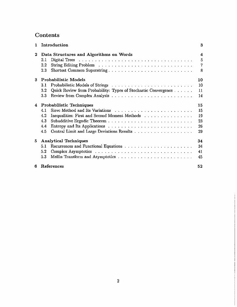
trio

'----'" 0

Patricia DST

Figure 1: A trie, Patricia trie and a digital search tree (DST) built from the following four

strings Xl = 11100. _. , X 2 = 10111. _. , X3 = 00110 ... , and X.i = 00001 ....

hence external nodes are eliminated. The branching policy is the same as in tries. Figure

2.1 illustrates these definitions.

The suffix tree and the compact sujJix tree are similar to the hie and PATRICIA tric,

but differ in the structure of the words that are being stored. In suffix trees and compact

suffix trees, the words arc suffixes of a given string X; that is, the word Xj = XjXj+1Xj+2 ...

is the suffix of X which begins at the j-th position of X. Thus a suffix tree is a trie and a

compact suffix tree is a PATIUCIA trie in which the words are all suffixes of a given string.

Certain characteristics of tries and suffix trees are of primary importance. Hereafter,

we assume that a digital tree is built from n strings or a suffix tree is constructed from a

string of length n. The m-depth Dn(m) of the m-th leaf in a trie is the number of internal

nodes on the path from the root to the leaf. The (typical) depth of the trie Dn then, is the

average depth over all its leaves, that is,

1 nPr{Dn S k} ~ - L Pr{Dn(m) S k} .

n m=l

The path length L n is the sum of all depths, that is,

n

Ln = L Dn(m).m=l

Closely related to the depth of a trie is the depth of insertion, which gives the depth of the

(n+l)-st key inserted into a trie ofn keys. The height Hn of the trie is the maximum depth

of a leaf in the trie and can also be defined as the length of the longest path from the root

to a leaf, that is,

6

The shortest path Sn of the trie is the length of the shortest such path. Finally, the size Sf!

of the trie is given by the number of internal nodes in the trie. These characteristics are

very useful in determining the expected size and shape of the data structures involved in

algorithms on words. We study some of them in this chapter.

2.2 String Editing Problem

The string editing problem arises in many applications, notably in text editing, speech

recognition, machine vision and, last but not least, molecular sequence comparison (d.

[97]). Algorithmic aspects of this problem have been studied rather extensively in the past

(d. [10, 76, 83, 97]). In fact, many important problems on words are special ca."les of

string editing, including the longest common subsequence problem (cf. [19, 16, 83]) and the

problem of approximate pattern matching (cf. [19]). In the following, we review the string

editing problem and its relationship to the longest path problem in a special grid graph.

Let Y be a string consisting of esymbols on some alphabet 2: ofsize V. There are three

operations that can be performed on a string, namely deletion of a symbol, insertion of a

symbol, and substitution of one symbol for another symbol in 2:. With each operation is

associated a weight function. We denote by WI(yt}, Wn(Yi) and WQ(Xi,Yj) the weight of

insertion and deletion of the symbol Yi E 2:, and substitution of Xi by Yj E 2:, respectively.

An edit script on Y is any sequence of edit operations, and the total weight of it is the sum

of weights of the edit operations.

The string editing problem deals with two strings, say Y of length l (for long) and

X of length s (for short), and consists of finding an edit script of minimum (maximum)

total weight that transforms X into Y. The maximum (minimum) weight is called the edit

distance from X to Y, and its is also known as the Levenshtein distance. In molecular biol­

ogy, the Levenshtein distance is used to measure similarity (homogeneity) of two molecular

sequences, say DNA sequences (cf. [83]).

The string edit problem can be solved by the standard dynamic programming method.

Let Cmax (i, j) denote the maximum weight of transforming the prefix of Y of size i into the

prefix of X of size j. Then, (cf. [10, 76, 97])

for aliI::; i ::; eand 1 ::; j S s. We compute Cmax(i,j) row by row to obtain finally the

total cost Cmax = Cmax(e, s) of the maximum edit script. A similar procedure works for the

minimum edit distance.

7

o w,

E

Figure 2: Example of a grid graph of size e= 4 and s = 3.

The key observation for us is to notc that interdependency among the partial optimal

weights Gmax(i,j) induce an ex s grid-like directed acyclic graph, called further a grid

graph. In such a graph vertices are points in the grid and edges go only from (i,j) point

to neighboring points, namely (i,j + 1), (i + 1,j) and (i + l,j + 1). A horizontal edge

from (i -1,i) to (i,j) carries the weight WI(Yj)i a vertical edge from (i,j -1) to (i,j) has

weight WO(Xi)i and finally a diagonal edge from (i - 1, j -1) to (i, j) is weighted according

to WQ(Xi,Yj). Figure 2 shows an example of such an edit graph. The edit distance is the

longest (shortest) path from the point 0 = (0,0) to E = (l, s).

Finally, we should mention that by selecting properly the distributions of Wj, WD and

WQ we can model several variations of the string editing problem. For example, in the

standard setting the deletion and insertion weights are identical, and usually constant,

while the substitution weight takes two values, one (high) when matching between a letter

of X and a letter of Y occurs, and another value (low) in the case of a mismatch (e.g., in

the Longest Common Substring problem [16, 831, one sets WI = WD = 0, and WQ = 1

when a matching occurs, and WQ = -00 in the other case).

2.3 Shortest Common Superstring

Various versions of the shortest common superstring (in short: SCS) problem play

important roles in data compression and DNA sequencing. In fact, in laboratories DNA

sequencing (cf. [66, 97]) is routinely done by sequencing large numbers of relatively short

fragments, and then heuristically finding a short common superstring. The problem can be

formulated as follows: given a collection of strings, say Xl, X 2 , • •. ,Xn over an alphabet E,

find the shortest string Z such that each of Xi appears as a substring (a consecutive block)

8

of Z.

It is known that computing the shortest common superstring is NP-hard. Thus con~

structing a good approximation to SCS is of prime interest. It has been shown recently,

that a greedy algorithm can compute in O(n log n) time a superstring that in the worst case

is only {3 times (where 2 :$ (3 :$ 4) longer than the shortest common superstring [13, 95].

Often, one is interested in maximizing total overlap of SCS using a greedy heuristic and

to show that such a heuristic produces an overlap o~r that approximates well the optimal

overlap o~Pt where n is the number of strings.

More precisely, suppose X = XIX2 ... X r and Y = Y!Y2 ... Ys are strings over the same

finite alphabet E. We also write IXI for the length of X. We define their overlap o(X, Y)

by

o(X, Y) = max{j : Yi = xr-Hl, 1:$ i:$ j}.

If X'" Y and k = o(X, Y), then

X EB Y = XIX2··· XrYk+lYk+2··· Ys'

Let S be a set of all superstrings built over the strings Xl, ... ,Xn. Then,

n

O~P' = I: IXiI - min IZI·i=l ZES

A generic greedy algorithm for the SCS problem can be described as follows: Its input

is the n strings Xl, X 2, ... , X n over E. It outputs a string Z which is a superstring of the

input.

Generic greedy algorithm

1. I {-- {Xl, X 2, X 3 , _ .. , Xn}j Or {-- 0;

2. repeat

3. choose X, Y E I; Z = X EB Y;

4. It- {l\ {X,Y}) U{Z};

5. Or {-- or + o(X, Y);

6. nntilill ~ 1

Different variants of the above generic algorithm can be envisioned by interpreting ap­

propriately the "choose" statement in Step 3 above. We shall discuss some probabilistic

aspects of it in sections below.

9

3 Probabilistic Models

In this section, we first discuss a few probabilistic models of randomly generated strings.

Then, we briefly review some basic facts from probability theory (e.g., types of stochastic

convergence), and finally we provide some elements of complex analysis that we sballu,se

in this chapter.

3.1 Probabilistic Models of Strings

As expected, random shape of data structures on words depends on the underlying proba­

bilistic assumptions concerning the strings involved. Below, we discuss a few basic proba­

bilistic models that one often encounters in the analysis of problems on words.

We start with the most elementary model, namely the Bernoulli model that is defined

as follows:

(B) BERNOULLI MODEL

Symbols oCthe alphabet E = {WI, ... ,wv} occur independently oCone another; thus, a

key X = XIX2X3 ••• can be described as the outcome of an infinite sequence of Bernoulli

trials in which Pr{xj = Wi} = Pi and EY=IPi = 1. If PI = pz = ... = pv = l/V, then

the model is called symmetric; otherwise, it is asymmetric. Throughout the paper

we only consider binaT1J alphabet ~ = {O, I} with p being the probability of "0" and

q = 1 - p the probability of "1" .

In general, when one deals with many strings (e.g., when building a digital tree) additional

assumption is made concerning the independence of the strings involved.

In many cases, assumption (B) is not very realistic. For instance, if the strings are words

from the English language, then there certainly is a dependence among the symbols oC the

alphabet. As an example, h is much more likely to follow an s than a b. When this is the

case, assumption (B) can be replaced by

(M) MARKOVIAN MODEL

There is a Markovian dependency between consecutive symbols in a keYi that is, the

probability Pij = Pr{Xk+l = WjlXk = wI} describes the conditional probability of

sampling symbol Wj immediately after symbol Wi.

There are two further generaliz~tionsof the Markovian model, namely mixing model and

the stationary model that are very useful in practice, especially when dealing with problems

10

of data compression or molecular biology when one expects long dependency among symbols

of a string.

(MX) MIXING MODEL

Let ~ be a a-field generated by {Xdk""m for m ::; n. There exists a function 0:(-)

of 9 such that: (i) limg--too o:(g) = 0, (ii) 0:(1) < 1, and (iii) for any m, and two events

A E~~ and B E ;:;;:+9 the following holds

(1- a(g))Pr{A}Pr{B} <: Pr{AB} <: (1 + a(g))Pr{A}Pr{B} .

In words, model (MX) says that the dependency between {Xdk=l and {Xdr""m+9 IS

getting weaker and weaker as 9 becomes larger (note that when the sequence {Xd is i.i.d.,

then Pr{AB} = Pr{A}Pr{B}). The "quantity" of dependency is charaderi:o:ed by o:(g) (d.

[11, 24]).

The most general probabilistic model that can provide some useful results, is the sta­

tionary model.

(8) STATIONARY MODEL

The sequence {Xdk=l of letters from a finite alphabet is a ,~tationary and ergodic

sequence of random variables.

To explain how the stationary model works, we need to introduce some notations. Let

X::l = (Xm, ... , Xn) for m < n, and let for every n 2: 1 the nth order probability distribution

for {Xd be P(Xf) = Pr{Xk = xk, 1::; k ::; n, Xk E A}. In the stationary model, this

probability does not depend on time·shift, that is, if T is an integer, then for every nand

T the following holds P(X1.t;) = P(Xf) (cf. [11, 24]).

3.2 Quick Review from Probability: Types of Stochastic Convergence

We begin with some elementary definitions from probability theory. The reader is refered to

(24, 25, 26, 85J for more detailed discussions. Let the random variable X n denote the value

of a parameter of interest depending on n (e.g., depth in a suffix tree and/or trie built over

n strings). The expected value E[Xnl or mean and the variance Var[XnJ can be computed

as E[Xnl ~ L~okPr{Xn ~ k} and Var[Xn]~ D"~o(k - E[Xn])'Pr{Xn = k}.

CONVERGENCE OF RANDOM VARIABLES. It is important to note the different ways in which

random variables are said to converge. To examine the different methods of convergence,

let X n be a sequence of random variables, and let their distribution functions be Fn(x),

11

respectively. A good and easy to read account on various types of convergence can be found

in Shiryayev [85].

The first notion of convergence of a sequence of random variables is known as conver­

gence in probability. The sequence X n converges to a random variable X in probability,

denoted X n -7 X (pr.) or Xn...!tX, if for any E > 0,

lim Pr{IXn -XI < ,j ~ 1.n~=

Note that tills does not say that the difference between X n and X becomes very small.

What converges here is the probability that the difference between X n and X becomes very

small. It is, therefore, possible, although unlikely, for Xn and X to differ by a significant

amount and for such differences to occur infinitely often.

A stronger kind of convergence which does not allow such behavior is called almost sure

convergence or strong convergence. A sequence of random variables X n converges to

a random variable X almost surely, denoted X n --t X (a.s.) or X n(~.)X, if for any E > 0,

lim Pr{sup IXn - XI < ,j ~ 1.N->oo n?N

From this formulation of almost sure convergence, it is clear that if Xn -7 X (a.s.), the

probability of infinitely many large differences between X n and X is zero. The sequence X n

in tltis case is said to satisfy the strong law of large numbers. As the term strong implies,

almost sure convergence implies convergence in probability.

A simple criterion for almost sure convergence can be inferred from the Borel-Cantelli

lemma. We give it in the following corollary.

Lemma 1 (Borel-Cantelli) Let E> O. If 2:~=oPr{IXIl - XI > E} < 00, then X n --t X

(a.s.).

Proof. It follows directly from the following chain of inequalities (the reader is referred to

Section 4.1 for more explanations on these inequalities):

Pr{sup IXn - XI'"' ,j ~ Pr{ U (IXn - XI,", ,n S L Pr{IXn - XI'"' ,j -+ 0 .n?N n?N n?N

The last convergence follows from our assumption that 2:~=oPr{IXn - XI > E} < 00.•

A third type of convergence is defined on the distribution functions Fn(x). The sequence

of random variables X n converges in distribution or converges in law to the random

variable X, denoted X n ~ X if

lim Fn(x) = F(x)n~=

12

for each point of continuity of F(x). Almost sure convergence implies convergence in dis­

tribution.

Finally, the convergence in mean of orderp implies that E[lXn -XIPj--7 0 as n -+ 00. It

is well known that almost sure convergence and convergence in mean imply the convergence

in probability. On the other hand, the convergence in probability leads to the convergence

in distribution. If the limiting random variable X is a constant, then the convergence in

distribution also implies the convergence in probability (d. [11, 24]).

GENERATING FUNCTIONS. The distribution of a random variable can also be described

using generating functions. The ordinary generating junction Gn(u), and a bivariate expo­

nential generating junction g(z, u) are defined as

G.(u)

g(z,u)

00

E[ux'J ~ L PriX. ~ k}uk ,

k==O

00 z.LG.(u),"n==O n.

These functions are well-defined for any complex numbers z and u such that lui < 1.

Observe that

- G~(1),

G~(I) + G~(I) - [G~(1)]2 "

LEVY'S CONTINUITY THEOREM. Our next step is to relate convergence in distribution

to convergence of generating functions. The following results, known as Levy's continuity

theorem is an archi-fact for most distributional analysis. For OUI purpose we formulate it

in terms of the Laplace transform of X n, namely Gn(Ct ) = E[e- tXn ) for real t.

Theorem 1 (Continuity Theorem) Let X n

transforms Gn(e-t ) and G(e- t ), respectively.

Xn~X is that Gn(e-t ) -+ G(e-t ) for all t ~ o.

and X be random variables with Laplace

A necessary and sufficient condition for

The above theorem holds if we set t = iv for -00 < 1I < 00 (i.e., we consider character­

istic functions). Moreover, if the above holds for t complex number, then we automatically

derive convergence in moments due to the fact that an analytical function possesses all its

derivatives.

Finally, a key result used in establishing central limit theorem (i.e., convergence to

a normal distribution) is a theorem by Goncharov (ef. [63], Chap 1.2.10, Ex. 13). This

13

theorem states that a sequence ofrandom variables X n with mean E[XnJ = tLn and standard

deviation an = JVar[Xnl approaches a normal distribution if the following holds:

lim e-TJJn/Un Pn(eT/Un) = eT2 / 2n~oo

for all T = iv and -00 < v < 00, and X n converges in moments if T is a complex number.

3.3 Review from Complex Analysis

Much of the necessary complex analysis involves the use of Cauchy's integral formula and

Cauchy's residue theorem. We briefly recall a few facts from analytical functions, and

then discuss the above two theorems. For precise definitions and formulations the reader is

referred to [44, 82]. We shall follow here Flajolet and Sedgewick [35J.

A function j(z) of complex variable z is analytical at point z = a if it is differentiable in

a neighbourhood of z = a or equivalently it has a convergent series representation around

z = a. Let us concentrate our discussion only on meromorphic functions that are analytical

with an exception of a finite number of points called poles. More formally, a meromorphic

function j(z) can be represented in a neighbourhood of z = a with z i- a by Laurent series

as follows:

I(z) = L: In(z - a)n ,n~-M

for some integer M. If the above holds with f-M i- 0, then it is ~aid that f(z) has a pole

of order M at z = a. Cauchy's Integral Theorem says that the coefficients f n of an

analytical function in a disk can be computed as

1 f dzIn ,~ [znlf(z) ~ 211"i I(z) zn+,

and the circle is traversed counterclockwise.

An important tool frequently used in the analytical analysis of algorithms is residue

thenry. The residue of j(z) at a point a is the coefficient of (z - a)-I in the expansion of

j(z) around a, and it is denoted as

Res[/(z); z ~ aJ ~ I-I

There are many simple rules to evaluate residues and the reader can find them in any

standard book on complex analysis (e.g., [44, 82]). Actually, the easiest way to compute

a residue of a function is to use the series commend in MAPLE that produces a series

development of a function. The residue is ~imply the coefficient at (z - a)-I. For example,

the following session of MAPLE computes series of j(z) = r(z)j(l - 2<:) at z = 0:

14

series(GAMMA(z)/(1-2-z), z=O, 4);

11 -7 - -In(2)

-2 2 -1-In(2) z - In(2) z-

1 1 1 1- (iln( 2)2 + 12,,2 + :2 72 + 4" (27 + In( 2) ) lo( 2)

In(2) +O(z)

From the above we see that Res[J(z); z = OJ = ~ +!.Residues are very important in evaluating contour integrals. In fact, a well-known

theorem in complex analysis, that 1s, Cauchy's residue theorem states that if f(z) is

analytic within and on the boundary of G except at a finite number of poles aI, a2, ... ,aN

inside of G having residues Res[J(z); z = al]"", Res[f(z); z = aN], then

Ni j(z)dz ~ 2"i L: Res[j(z); z ~ aj] ,C j=l

where the curve C is traversed counterclockwise.

4 Probabilistic Techniques

In this section we discuss several probabilistic techniques that have been successfully applied

to the average case analysis of algorithms. We start with some elementary inclusion­

exclusion principle known also as sieve methods. Then, we present very useful first

and second moment methods. We continue with the subadditive ergodic theorem

that is quite popular for deducing some properties of problems on words. Next, we turn

our attention to some probabilistic methods of information theory, and in particular we

discuss entropy and asymptotic equipartition property. Finally, we look at some

large deviations results and Azuma's type inequality. In thls section, as well in

the next one where analytical techniques are discussed, we adopt the following scheme of

presentation: First, we describe the method and give a short intuitive derivation. Then, we

illustrate it on some non-trivial examples taken from the problems on words discussed in

Section 2.

4.1 Sieve Method and Its Variations

The inclusion-exclusion principle is one of the oldest tools in combinatorics, number theory

(where this principle is known as sieve methorI), discrete mathematics, and probabilistic

15

analysis. It provides a tool to estimate probability of a union of not disjoint events, say

Ui~l Ai where Ai are events for i = 1, ... ,n. However, before we plunge into our discussion,

let us first show a few examples of problems on words for which an estimation of the

probability of a union of events is required.

Example 1: Depth and Height in a Trie

In Section 2.1 we discussed tries built over n binary strings Xl, ... ,XT/.' We assume

that those strings are generated according to the Bernoulli model with one symbol, say "0",

occurring with probability p and the other, say "1", with probability q = 1 - p. Let Cij,

known as alignment between ith and jth strings, be defined as the length of the longest

string that is a prefix of Xi and Xj. Then, it is easy to see that the mth depth Dn(m) (Le.,

length of a path in trie from the root to the external node containing X m ), and the height

H n (Le., the length of the longest path in a trie) can be expressed as follows:

max {C,m}+I,l:::;#m:::;n '

max {Cij} + 1.l:::;i<j:::;n

(1)

(2)

Certainly, the alignments Gij are dependent random variables even for the Bernoulli model.

The above equations expressed the depth and the height as an order statistic (i.e., maximum

of the sequence Ci,j for i,j = 1, ... ,n). We can estimate some probabilities associated with

the depth and the height as a union of properly defined events. Indeed, let Aij = {Gij > k}

for some k. Then, one finds

nPr{Dn(m) > k} - Prj U Ai,m} , (3)

i=l,:;lm

nPr{Hn > k} ~ Prj U AiJ } (4)

i,j=l

In passing, we should point out that for the Shortest Common Superstring Problem (d.

Section 2.3) we need to estimate a quantity Mn(m) which is similar to Dn(m) except that

Gim is defined as the length of the longest string that is a prefix of Xi and suffix of X m for

fixed m. One easily observes that Mn(m) 4 Dn(m), that is, these two quantities are equal

in distribution. 0

We have just seen that often we need to estimate a probability of union of events. The

following formula is known as inclusion-exclusion formula (d. [12])

n n

Pr{U Ai} ~ 2)-1)'+1 L: Pr{ nAj } . (5)i=l r=l IJI=r jEJ

16

The next example illustrates it on the depth on a trie.

Example 2: Generating Function of the Depth in a The

Let us compute the generating function of the depth Dn := D n (1) for the first string

Xl. We start with (3), and after some algebraic manipulation (5) leads to (cf. [51, 52])

Pr{DIl 2: k}n

Pr{ U[Ci,1 ~ kJ}1=2

~ ~ I=(-lr (n)pr{C2" ~k, ... ,C;,1 ~k}n r=2 r

since the probability Pr{C2,1 2: k, ... , Cr ,1 2: k} does not depend on the choice of strings

(i.e., it is the same for any r-tuple of strings selected). Moreover, it can be easily explicitly

computed. Indeed, we obtain

since r independent strings must agree on the first k symbols. Thus, the generating function

Dn(u) = EuD" becomes

_l_I-Z~(_lr(n)r 1- n ~ r 1 - z(pr + qr) .

The last formula is a simple consequence of the above, and the following well known fact

from the generating function Eux for a random variable X:

. 1 00

Eu" ~ -- L PriX '" k}uk

1 - U k=O

o

In many real computations, however, one cannot explicitly compute the probability of

the events union. Often, one must retreat to inequalities that actually are enough to reach

one's goal. The most simple yet still very powerful is the following inequality

n n

Pr{ UAi} '" L Pr{Ai } .i=1 i=1

(6)

The latter is an example of a series of inequalities due to Bonferroni which can be formulated

as follows: For every event integer e 2: 1 we have,L L Pr{A t , n .. · nAt,} '"p=1191S .. ·-::;LpSn

n

Pr{ UAi}i=1

,:-:; L L Pr{ALI n .. ·nAlp+J.

p=1191S ""S!pSn

17

In combinatorics (e.g., enumeration problems) and probability the so called inclw;ion­

exclusion principle is very popular and had many successes. We formulate it in a form of a

theorem whose proof can be found in Bollobas [12].

Theorem 2 (Inclusion-Exclusion Principle) Let AI,"" An be events in a probability

space, and let Pk be the probability of exactly k of them to occur. Then:

Example 3: Computing a Distribution Through Its Moments

Let X be a random variable defined on {O,l, ... , n}, and let Er[X] = EX(X -1)··' (X­

r + 1) be the rth factorial moment of X. Then:

P,{X = k} = ~ ~(-1)* E,[Xjk! L, (r k)!r,="k

Indeed, it suffices to set Ai = {X 2: i} for all i = 1, ... , n, and observe that 2::1J1,="r Pr{njEJ Aj } =

Er[X]/r!. Since the event {X = k} is equivalent to the event that exactly k of A occur, a

simple application of Theorem 2 proves the announced result. 0

Finally, we say a few words about the so called Lovasz Local Lemma (cf. [5, 12, 75])

which can be Himply stated as follows: If there are n mutually independent (bad) events Bi

each of probability strictly smaller than one, then there i.<; a positive probability that none of

the bad events happens. We shall formulate this in a more precise manner below. It Hhould

be clear, however, from the above that this lemma can be used to prove the existence of

some complicated structure by showing that it must occur with a positive probability.

Let us start with a simple statement. If 2::i,=,,1 Pr{B j } < 1, then Pr{ni~IEJ > O.

Indeed,n n n

p,{n Hi} ~ 1- P,{U Ai} ~ 1- LP,{Bi} > 0t,="l i,="l i,="l

where the first inequality follows from Bonferroni's inequality (6).

A stronger statement is in fact true. First of all, let us notice that if Pr{Bi} < 1 and

all n events are mutually independent, then Pr{nf,="l Bi } > O. Indeed, it suffices to observe

that Pr{ni,="l B i } = ITi,="d1 - Pr{Bd) > O. Erdos and Lovasz (d. (12]) proved that the

above conclusion is true even if there is some dependency among the events. For example:

let every d events be dependent and let Pr{Bi } :::; P for all i = 1, ... , n such that 4dP < 1.

Then, Pr{ni,="l EJ > O. The reader is referred to [5, 12) for a more general formulation of

this lemma, and for interesting applications.

18

4.2 Inequalities: First and Second Moment Methods

In this subsection, we review some inequalities that playa considerable role in probabilistic

analysis of algorithms. In particular, we discuss first and second moment methods that are

"bread-and-butter" of a typical probabilistic analysis.

We start with a few standard inequalities (cf. [24, 85]):

Markov Inequality: For a nonnegative random variable X and E > 0 the following holds:

Indeed: let leA) be the indicator function of A (Le., leA) = 1 if A occurs, and zero

otherwise). Then,

E[X] 2 E[XI(X 2 E)] 2 EE[I(X 2 Ej] ~ EPr{X 2 EJ .

Chebyshev's Inequality: If one replaces X by IX - E[X]I in the Markov inequality, then

Schwarz's Inequality (also called Cauchy-Schwarz): Let X and Y be such that E[X2] <00 and E[y2] < 00. Then:

EIIXYI]' " E[X']E[Y'] ,

where E[X]' ,~ (E[X])'.

Jensen's Inequality: Let f(-) be a downward convex function, that is, for).. E (0,1)

Af(x) + (1- A)f(y) 2 f(AX + (1- A)Y) .

Then:

f(E[X]) " EIJ(X)] .

The remainder part of this subsection is devoted to the first and the second moment

methods that we illustrate on several examples arising in the analysis of digital trees. The

first moment method for a nonnegative random variable X boils down to

PriX > OJ "E[X) . (7)

This follows directly from Markov's inequality after setting E = 1. The above inequality

implies also the basic Bonfferroni inequality (6). Indeed, let Ai (i = 1, ... ,n) be events,

and set X ~ I(Ad + ... + I(An ). Inequality (6) follows.

19

In a typical usage of (7), we expect to show that E[X] -t 0, just X = 0 occurs almost

always or with high probability (whp). We illustrate it in the next example.

Example 4: Upper Bound on the Height in a Trie

In Example 1 we showed that the height Hn of a trie is given by (2) or (4). Thus, using

the first moment method we have

for any integer k. From Example 2 we know that Pr{Cij 2. k} = (p2+ q2)k. Let P = p2+ q2,

Q = p-l, and set k = 2(1 + e) logQ n for any e > O. Then, the above implies

thus Hn /(2IogQ n) ::; 1 (pr.). In the example below, we will actually prove that Hn /(2IogQ n) =

1 (pr.) by establishing a lower bound. 0

Let us look now at the second moment method. Setting in the Chebyshev inequality

to = E[X] we easily prove that

VariX]Pr{X ~ O} '" E[X)' .

But, one can do better (cE. [5,17]). Using Schwar:.-.'s inequality for a random variable X we

obtain the following chain of inequalities

E[X]' = E[I(X # O)X]' '" E[I(X # O)]E[X'] ~ Pr{I(X # O)}E[X'] ,

which finally implies the second moment inequality

E[X)'PriX > O} 2 E[X'] . (8)

Actually, another formulation of this inequality due to Chung and Erdos is quite popular.

To derive it, set in (8) X = I(A1) + ... +I(An) for a sequence of events AI, ... , An. Noting

that {X > O} = Ui=lA j , we obtain after some algebra

(9)

In a typical application, we are able to prove that Var[X]/E[X2] -t 0, thus showing

that {X > O} almost always. The next example - which is a continuation of Example 4­

illustrates this point.

20

Example 5: Lower Bound fOT the Height in a Trie.

We now prove that Pr{Hl1 ~ 2(1- c) logQ n} -+ 1, just completing the proof that

Hn/(2IogQ n) -+ 1 (pr.). We use the Chung~Erd6s formulation, and set Aii = {Gii ~ k}.

Throughout this example, we assume k = 2(1-£) logQn. Observe that now in (9) we must

replace the single summation index i by a double summation index (i,j). The following is

obvious

L P,{Aij } = ~n(n - 1)pk ,I5i<i5n

where P = p2 + q2. The other sum in (9) is a little harder to deal with. We must sum over

(i,j), (l,m), and we consider two cases: (i) all indices are different, (ii) i = 1 (i.e., we have

(i,j), (i,m)). In the second case we must consider the probability Pr{Cii ~ k,Gi,m ~ k}.

But, as in Example 2, we obtain Pr{Gij ~ k, Ci,m 2. k} = (p3 + q3)k since once you choose

a symbol in the string Xi you must have the same symbol on the same pm,ition in Xi, X m .

In summary,

" P,{C·· > k C, > k} < ~n'p2k +n3(p3 +q3)k .L...J 11_' m_ -4(ij),(l,m)

We need a simple inequality that can be easily verified (see [55, 7] for a more elaborate

extension), namely:

Then, (9) becomes

1

>

"P,{H" ~ k} = P,{U Ai} >

i=1n 2p k+1+4(p3+ q3)kf{nP2k)

1 > 11 +n 2£" + 4/(nPk/2) - 1 + n 2£" + 4n £" -+ 1 .

Thus, we have shown that Hn/(21ogQ n) 21 (pr.), which completes OUI proof of

for any E > O. D

We complete this subsection with two results concerning order statistics that find plenty

of applications in average case analysis of algorithms. These results are direct consequences

of the methods discussed here, but for completeness we give a short derivation (d. [4, 38]).

Lemma 2 Let YI, Y2, ... ,Ym be a sequence of random variables with distribution functions

FI (y), F2(y) , ... , Fm(y), respectively. Let .n.(y) = Pr{Yi ~ y} be the complement function

of the distribution function Fi(Y)· Define Mm = maxt<i<m{Yi}.

21

(i) If am is the smallest solution of

m

L R.(am) = 1 ,k=1

thenm 00

E[Mml 5: am + L L Rdj) .k=1 j=am

(10)

(ii) If dist1ibution Junctions Fi (y) of Y1 , Y2, _.. ,Ym satisfying for all 1 ~ i ~ m the following

two condition,<;

and

F;(y) < 1 for all y<oo,

lim sup 1- Fi(CY) = a for c> 1 ,Y-tOO i 1 - Fi(Y)

then Mm/am :::; 1 in probability (pr.), that i,<;, for any c > a

(11)

where am ,<;olve,<; a,<;ymptotically (10).

(iii) If Yj, ... , Ym are independently and identically di,<;tributed (i.e., i.i.d.) with common

distribution function F(·), then M m '" am (pr.), that i,<;, for any c > a

lim Pr{(l- clam :::; M m .:S (1 + clam} = 1,m~oo

where am is a solution of (10) which in this ca!.e becomes mR(am) = 1.

Proof. For (i) observe that, for any a,

m

M m 5: a + L[Y' - aJ+k=l

where t+ denotes max{O, t}. Since [Yk - a]+ is a nonnegative random variable, then

E[Yk - a]+ = faoo Rk(y)dy, so that (assuming for simplicity that Yi is a continuous random

variable)

E[MmJ 5: a + f:100

Rdx)dx .k=1 a

Minimizing the right-hand side of the above with respect to a yields part (i). For part (ii)

we apply inequality (6) to get

m

Pr{Mm > x} = Pr{Yl > x, or , .... , or ,Ym > x}:::; L:.R>(x).i=1

22

Let x = (l+c)am where f: > 0 and am be defined by (10). Then1(11) with c = l+c implies

R(I + <lam) ~ o(I)R(am), hence

m

PrIMm ?' (I + clam) ~ 0(1) L R(am) ~ 0(1) .i=l

Finally, part (iii) can be proved using the additional assumption about the independence

ofYl1···,Ym· •

In certain applications, we are interested not only in the maximum value but the r·th

maximum value of the sequence Yl1 ... ,Ym. Let mint:Si:5m {Yi} = 1(1) :$; 1(2) :$; ... :$; Y(m) =

maxl-::;i-::;m, and we call Y(r) the rth order statistics of Y1 , ... , Ym . Below, we present a simple

asymptotic result concerning the behavior of Y(r) for the so called exchangeable random

variables. A sequence {Yi}~1 is exchangeable iffor any k-tuple {jt, ... ,id of the index set

{l, ... ,m} the following holds: Pr{1'jl < Yil,···,Yjk < Yik} = Pr{YI < Yl, ... ,Yk < Yk},

that is, the joint distribution depends only on the number of variables (cf. [38]).

Lemma 3 Let {Yi}kl be exchangeable random variables, and let R(r)(x)

X, ... , Yr > x} satisfies (H). Define a~) as the smallest solution of

Pr{Y, >

Then, M(r) ::; a~) (pr.). If, in addition, Yi are i.i.d., then M(r) ,..... a~) (pr.) for m ----t 00.

Proof. One should apply inequality (6) to Pr{MZ) > x} = Pr{UJI, ..,jm_~+In~lr+l(Yji >yn for all distinct il, ... ,im-r+1 E {I, ... ,m}.•

4.3 Subadditive Ergodic Theorem

The celebrated ergodic theorem of Birkhoff [25, 26] found many useful applications in com­

puter science. It is used habitually during a computer simulation run or whenever one must

perform experiments and collect data. However, for probabilistic analysis of algorithms a

generalization of this result due to Kingman [58] is more important. We briefly review it

here and illustrate on a few examples.

Let us start with the following well known fact: Assume a (deterministic) sequence

{xn}~=o satisfies the so called subadditivity property, that is,

23

for all integers m,n';::: o. It is easy to see that then (cf. [24])

, . Xn - r "m1m - = In - =e>n-HlO n m~1 m

for some a E [-00,00). Indeed, it suffices to fix m 2 0, write n = km+l for some 0 S; I ::; m,

and observe that by the above subadditivity property

Taking n --t 00 with njk --t m we finally arrive at

X n X mlimsup- S - S; a,n--)oo n m

where the last inequality follows from arbitrariness of m. This completes the derivation

since

li . r"nmm ->e>n-Jooo n -

is automatic. One can also see that replacing "s;" in the subadditivity property by">"

(thus, supemdditivity properly) will not change OUI conclusion except that infm>1 ~ should_ m

be replaced by sUPm~1 ~.

In the early seventies people started asking whether the above deterministic subaddi­

tivity result could be extended to a sequence of random variables. Such an extension would

have an impact on many research problems of those days. For example, Chvatal and Sankoff

[16] used ingenious tricks to establish the probabilistic behavior of the Longest Common

Superstring problem (cf. Section 2.2 and below) while we show below that it is a trivial

consequence of a stochastic extension of the above subadditivity result. In 1976 Kingman

[58] presented the first proof of what later will be called Subadditivity Ergodic Theorem.

Below, we present an extension of Kingman's result.

To formulate it properly we must consider a sequence of of doubly-indexed random

variables Xm,n with m ::; n. One can think of it as Xm,n = (Xm,Xm+l,"" X n), that is, as

a substring of a single-indexed sequence X n .

Theorem 3 (Subadditive Ergodic Theorem) (i) Let Xm,n (m < n) be a sequence of

nonnegative mndom variables satisfying the following three properties

(a) XO,n S; XO,m + Xm,n (subadditivity),-

(b) Xm,n is stationary (i.e., the joint distributions of Xm,n are the same as Xm+l,n+l)

and ergodic (ef. {II]};

24

(e) E[Xo,,J < 00.

Then,lim E[Xo,n) ~?

n-lOO n

for some constant 'Y.

and lim XO,n = 'Y (a.s.)n--+= n

(12)

(ii) (Almost Subadditive Ergodic Theorem [21]) If the subadditivity inequality is re­

placed by

XO,n ~ XO,m + Xm,n + An

such that limn--+= E[An/n] = 0, then (12) holds, too.

(13)

We must point Dut, however, that the above result proves only the existence of a constant

i such that (12) holds. It says nothing how to compute it, and in fact many ingenious

methods have been devised in the past to bound this constant. We discuss it in a more

detailed way in the examples below_

Example 6: String Editing Problem

Let us consider the string editing problem of Section 2.2. To recall, one is interested in

estimating the minimum Cmill or the maximum cost Cmax of transforming one sequence into

another. In a particular case (i.e., Longest Common Superstring problem) one selects the

longest common superstring of two given strings. As mentioned in Section 2.2 this problem

can be reduced to finding the longest (shortest) path in a special grid graph (cf. Figure 2).

Let us assume that the weights WI, WD and WQ are independently distributed, thus we

adopt the Bernoulli model (B) of Section 3.1. Then, using the subadditive ergodic theorem

it is easy to prove that for some constant a > a

li Cm~ li ECmiU ()m -- = m = a a.s.,n-t= n n--+oo n

provided eJs has a limit as n --Jo 00. Indeed, let us consider the I!. x oS grid with starting point

o and ending point E (cf. Figure 2). Call it Grid(O,E). We also choose an arbitrary point,

say A, inside the grid so that we can consider two grids, namely Grid(O,A) and Grid(A,E).

Actually, point A splits the edit distance problem into two subproblems with objective

functions Cmax(O,A) and CmiU(A,E). Clearly, CmiU(O,E) ~ CmiU(O,A) + CmiU(A,E).

Thus, under our assumption regarding weights, the objective function Cmax: is superadditive,

and direct application of the Superadditive Ergodic Theorem proves the result.

We should observe, however, that the above result does not tell us how to compute a.

In fact, even in the simplest ca.se of the Longest Common Superstring problem the constant

a is unknown, but there are some bounds on a (cf. [16, 83]). 0

25

4.4 Entropy and Its Applications

Entropy and mutual information was introduced by Shannon in 1948, and over a night

a new field of information theon) was born. Over the last fifty years information theory

underwent many changes, and remarkable progress was achieved. These days entropy and

the Shannon-McMillan-Breiman Theorem are standard tools of the average case anal­

ysis of algorithms. In thls subsection, we review some elements of information theory and

illustrate its usage to the analysis of algorithms.

Let us start with a simple observation: Consider a binary sequence of symbols of length

n, say (Xl, ... ,Xu), with p denoting the probability of one symbol and q = 1 - p the

probability of the other symbol. When p = q = 1/2, then Pr{XI , ... , Xn} = 2-u and it

does not matter what are the actual values of Xl, ... , Xn. In general, Pr{XI , ... , Xn} is

not the same for all possible values of Xl, ... , Xn, however, we shall show that a typical

sequences (XI, .. _, Xn) have "asymptotically" the same probability. Indeed, consider p i- q

in the example above. Then, a typical sequence has the probability of its occurrence (we

use here the ccntrallimlt theorem for i.i.d. sequences):

where h = -p logp-q log q is the entropy of the underlying Bernoulli model. Thus, a typical

sequence Xf has asymptotically the same probability equal to e-nh .

To be more precise, let us consider a stationary and ergodic sequence {Xdgl (cf.

Section 3.1), and define X~ = (Xm,Xm+I, ... , Xn) for m ::; n as a substring of {Xdk=l.

The entropy h of {Xdk::l is defined as (d. [11, 18, 24])

h,~ - lim E[logP,{Xf}] (14)n---)oo n

where one can prove the limt above exists. We must point out that Pr{Xf} is a random

variable since Xr is a random sequence!

We show now how to derive the Shannon-McMillan-Breiman theorem in the case of

the Bernoulli model and the mixing model, and later we formulate the theorem in its full

generality. Consider first the Bernoulli model, and let {Xd be generated by a Bernoulli

source. Thus

log Pr{Xf}n

1 n

-- I)og P,{X,}n i=l

--> E[-logP,{Xdl = h (a.s.) ,

where the last implication follows from the Strong Law of Large Numbers (cf. [11]) applied

to the sequence (-log Pr{XI }, ... , -log Pr{Xn}). One should notice a difference between

26

the definition of the entropy (14) and the result above. In (14) we take the average. of

log Pr{Xf} while in the above we proved that almost surely for all but finitely sequences

the probability Pr{Xf} can be closely approximated by e-nh . For the Bernoulli model l we

have already seen it above, but we are aiming at showing that the above conclusion is true

for much more general probabilistic models.

As the next step, let us consider the mixing model (MX) (that includes as a special case

the Markovian model (M». For the mixing model the following is true:

for some constant c> 0 and any integers n, m ;::: O. Taking logarithm we obtain

log Pr{X1+m} ::; log Pr{Xr} + log Pr{X:ti} + loge

which satisfies the subadditivity property (13) of the Subadditive Ergodic Theorem discussed

in Subsection 4.3. Thus, by (12) we have

h ~ _ lim log Pr{XrJn--+oo n

(a.s.) .

Again, the reader should notice the difference between this result and the definition of the

entropy.

We are finally ready to state the Shannon-McMillan-Breiman in its full generality (d.

[11, 24]).

Theorem 4 (Shannon-McMillan-Breiman) For a stationanj and ergodic sequence {Xd~_oo

the following holds

I· ,I.o:;,ge:-Pe:-r{~X:!f~}h=- Im-n--+oo n

where h is the entropy of the process {Xd.

(a.s.) .

An important conclusion of this result is the so called Asymptotic Equipartition

Property (AEP) which basically asserts that asymptotically all sequences have the same

probability approximately equal to e-nh . More precisely:

For a stationary and ergodic sequence Xf I the state space :En can be partitioned

into two subsets B~ (i'bad set n) and g~ ("good set") such that for given c > 0

there is Ne so that for n;::: Ne we have Pr{B~} ::; c, and cnlt(l+e) ::; Pr{xr} ::;e-nh(l-e) for all xr E g~.

27

o

Example 7: Shortest Common Superstring or Depth in a The/Suffix Tree

For concreteness let us consider the Shortest Common Superstring discussed in Sedion

2.3, but the same arguments as below can be used to derive the depth in a trie (cf. [79]) or

a suffix tree (cf. [91]). Define Gij as the length of the longest suffix of Xi that is equal to

the prefix of Xj. Let

M.(i) = max .{C'j}.1:5,:511.:1#'

We write M l1 for a generic random variable distributed as M l1 (i) (observe that M n4Mn (i)

for all i, where 4 means "equal in distribution"). We would like to prove that in the mixing

model, for any £ > 0

lim Pr {(1- o)-hlI0gn S M. S (1 + o).!.IOgn} ~ 1 - O(I(n')71-1-00 h

provided a(g) --) 0 as 9 --+ 00, that is, Mnj log n ----+ h (pr.). To prove an upper bound, we

take any fixed typical sequence Wk E gk as defined in AEP above, and Dbserve that

The result fDllDws immediately after substituting k = (1 + £)h-1 10gn and nDting that

Pr{wd S e nh(1-e-). FDr a lDwer bDund, let Wk E gf be any fixed typical sequence with

k = *(1 - £) lDgn. Define Zk as the number of strings j t- i such that a prefix Df length

k is equal tD Wk and a suffix of length k Df the ith string is equal to Wk E gk. Since Wk is

fixed, the random variables Cij are independent, and hence by the second moment method

(cf. Section 4.2)

VarZk 1 2

PrIM. < k} ~ Pr{Zk ~ O} S ( )2 S P { } = O(n-' ) ,EZk n r Wk

since VarZk S nP(wk), and this completes the derivation.

In many problems on words another kind of entropy is widely used (cf. [7, 8, 9, 91]). It

is called Renyi entropy and defined as follows: For -00 S b S 00, the bth order Re.nyi

entropy is

provided the above limit exists. In particular: by inequalities on means we obtain

ho

h-oo

h,lim _m_ax_{,--_lo",g_P_r{,-X~f...,},--,--,P_r-,,{X,-,,-f.<-}-,->_O,-,-}

n---Joco n

lim "m"in"'{c.---""'og"-'--P"r{-'-X"f2}--',-'-P-'-r{"X.:.f...,}'-.:.->--'O"-}n-l-OO n

28

For example, the entropy h_ oo appears in the formulation of the shortest path in digital

trees (cf. [79, 91]), the entropy hco is responsible for the height in PATRlCIA tries (d.

[79, 91]), whilc h2 determines the height in a trie. Indeed, we claim that in a mixing model

the height Hn in a trie behaves probabilistlcally as Hn/logn --+ 21h2 • Consider first the

Bernoulli model as in Examples 4 and 5. Using oUI definition of h2 in the Bernoulli model

one immediately proves that h2 = logP-l = logQ where P = p2+ q2 as defined in Example

4. This confirms our observation. An extension to a mixing model follows the footsteps of

our proof from Examples 4 and 5 and can be found in [79, 90, 91]'

4.5 Central Limit and Large Deviations Results

Convergence of a sum of independent, identically distributed (Li.d.) random variables is

central to probability theory. In the analysis of algorithms, we mostly deal with weakly

dependent random variables, but often results from the i.i.d. case can be cxtended to this

new situation by some clever tricks. A more systematic treatment of such cases is usually

done through generating functions and complex analysis techniques (cf. [32,48,49, 51, 52,

53,73]) which we briefly discuss it in the next section. Hereafter, we conccntrate on the

i.i.d. case.

Let us consider a sequence Xl,"" X n of i.i.d. random variables, and let 8n = Xl +... + Xn. Define J.L := E[XI] and 0-

2 := Var[XIJ. We pay particular interest to another

random variable, namely8n - nJ.L

8 n := --"---,""-",fii

which distribution function we denote as Fn(x) = Pr{8n ::; x}.

distribution function of the standard normal distribution, that is,

Let also ID(x) be the

The Central Limit Theorem asserts that Fn(x) --t l1>(x) for continuity points of Fn(-),

provided a < 00 (cf. [24, 26]). A stronger version is due to Berry-Esseen who proved that

2pIFn(x) - <I'(x)1 S 2 r.;;

" yn(16)

where p = E[IX - J.L1 3) < 00. Finally, Feller [26] has shown that if centralized momcnts

J.L2, .•. ,J.Lr exist, then

29

uniformly in x, where Rk(X) is a polynomial depending only on 11-1, ... ,l1-r but not on nand

T.

One should notice from the above, in particular from (16), the weakness of central limit

results which are able only to assess the probability of small deviations from the mean.

Indeed, the results above are true for x = 0(1) (i.e., for 8Tl E (/l-n- O(.Jii),/l-n + O(vn))

due to only a polynomial rate of convergence as shown in (16). To see it more clearly, we

quote a result from Greene and Knuth [40] who estimated

(17)

where ~3 is the third cumulant of Xl. Observe now that when r = O(.jn) (which is

equivalent to x = 0(1) in our previous formulce) the error term dominates the leading term

of the above asymptotic, thus the estimate is quite useless.

From the above discussion, one should conclude that the central limit theorem has

limited range of application, and one should expect another law for large deviations from

the mean, that is, when Xn. --7 00 in the above formulce. The most interesting from

the application point of view is the case when x = O(J1i) (or r = O(n)), that is, for

Pr{8n. = n(/l- + on for 0 f. O. We shall discuss this large deviations behavior next.

Let us first try to "guess" a large deviation behavior of 8n = Xl + ... X n for i.i.d.

random variables. We estimate Pr{8n ~ an} for a > 1 as n --7 00. Observe that (d. [24]

Pr{Sn.+m ~ (n+m)a} ~ PriSm ~ rna, 8n.+m - 8m ~ na} = Pr{8n ;::: na}Pr{Sm:::::' rna}

since 8m and 8n.+m - 8 m are independent. Taking logarithm of the above, and recognizing

that log Pr{Sn:::::' an} is a superadditive sequence (cf. Subsection 4.3), we obtain

1lim -logPr{Sn~na}~-I(a)n~oo n

where 1(a) 2: O. Thus, 8n. decays exponentially when far away from its mean, not in a

Gaussian way as the central limit theorem would predict! Unfortunately, we obtain the

above result from the subadditive property which allowed us to conclude the existence of

the above limit, but says nothing about 1(a).

In order to take a full advantage of the above derivation, we should say something about

1(a) and, more importantly, to show that 1(a) > 0 under some mild conditions. For the

latter. let us first assume that the moment genemting function

M(>.) = E[e.\X1 ] < 00 for some>' > O.

30

Let also x;(.\) = logM(A) be the cumulant function of Xl. Then, by Markov's inequality

(cf. Subsection 4.2)

Actually, due to arbitrariness of A subject to .\ > 0, we finally arrive at the so called

Chernoff bound, that is,

(18)

We should emphasize that the above bound is true for dependent random variables since we

only used Markov's inequality applied to S'l·

Returning to the i.i.d. case, we can rewrite the above as

P,{Sn > na} $ min {exp(-n(aA - K(a)))- ),>0

But, under mild conditions the above minimization problem is easy to solve. One finds that

the minimum is attended at Aa which satisfies a = M'(Aa)jM(Aa). Thus, we proved that

I(a) ;::: aAa -logM(Aa ). However, a careful evaluation of the above leads to the following

c1assicallarge deviations result (cf. [24])

Theorem 5 Assume X I1 ... , X n are i.i.d. Let M(...\) = E[e),x1 ] < 00 for !lome A> 0, the

distribution of Xi is not a point mass at fJ-, and there exist!l Aa > 0 in the domain of the

definition of M(A) such that

Then:. 1

hm -logPr{Sn;::: na} = -(aAa -logM(.\a))n--Jco n

for a > fJ-.

A major strengthening of this theorem is due to mutner and Ellis who extended it to

weakly dependent random variables. Let us consider Sn as a sequence of random variables

(e.g., Sn = Xl + ... + X n), and let Mn(A) = E[e)'Sn]. The following is known (d. [22]):

Theorem 6 (Gartner-Ellis) Let

lim log Mn(A) = c(A)n--Jco n

exist and is finite in a subinterval of the real axis. If there exists Aa such that d(...\a) is finite

and c'(Aa) = a, then

31

Let us return again to the i.i.d. case and see if we can strengthen Theorem 5 which in its

present form gives only a logarithmic limit. We explain our approach on a simple example,

following Greene and Knuth [40]. Let us assume that Xl, ... , Xf! are discrete i.i.d. with

common generating function G(z) = E[zX]. We recall that [zm]G(z) denote the coefficient

at zTll of G(z). In (17) we show how to compute such a coefficient at m = JLn + O(vn) of

Gn(z) = Ezs". We observed also that (17) cannot be used for large deviations since the

error term was dominating the leading term in such a case. But, one may shift the mean of

Sn to a new value such that (17) is valid again. Thus, let us define a new random variable

X whose generating function is

G-( ) ~ G(za)z G(a)

where a is a constant that is to be determined. Observe that E[X] = 0"(1) = aG1(a)/G(a).

Assume one needs large deviations result around m = n(M + 8) where 8 > O. Clearly, (17)

cannot be applied directly. Now, a proper choice of a can help. Let us select a such that

the new Sn = Xl + ... + Xn has mean m = n(p, + 8). This results in setting a to be a

solution ofaG1(a) _ m _ l'

G(a) - n - I' + v .

In addition, we have the following obvious identity

(19)

But, nOw we can use (17) to the right-hand side of the above since the new random variable

Sf! has mean around m.

To illustrate the above technique that is called shift of mean we present an example.

Example 8: Large Deviations by "Shift of Mean" (cf. [40]).

Let Sn be be binomially distributed with parameter 1/2, that is, Gn(z) = ((1 + z)/2)n.

We want to estimate the probability Pr{Sn = n/3} which is far away from its mean (ESn =

n/2) and central limit result (17) cannot be applied. We apply shift of mean, and compute

=l+a 3'

aasaG'(a)G(a)

thus, a = 1/2. Using (17) we obtain

a 1

[ n/3j (2 1) n 3 ( 7 ) -5/2Z - + -z = -- 1 - - + O(n ) .3 3 2y0ffi 24n

32

To obtain the result we want (i.e., coefficient at znj3 of (z/2 + 1/2)n), one must apply (18).

This finally leads to

(3 21/3)" 3 (7 )[zn/3](z/2 + 1/2)" =' -- 1 - - + O(n-')

4 2y'iFii 24n

which is a large deviations result (the reader should observe the exponential decay of the

above probability). 0

The last example showed that one may expect a stronger large deviation result than the

one presented in Theorem 5. Indeed, under proper mild conditions it can be proved that

Theorem 5 extends to (cf. [22])

1Pr{S";:> na} - m= exp(-nI(a))

v 2nna(1)'(1

for a constant aa, and ,\(1 and I(a) = a>'(1 -logM(>,(1) defined as in Theorem 5.

Finally, we deal with an interesting extension of the above large deviations results ini­

tiated by Azuma, and recently significantly extended by Talagrand [93J. These results

are known in the literature under the name Azuma's type inequality or method of

bounded differences (cf. [74]). It can be formulated as follows:

Theorem 7 (Azuma's type Inequality) Let Xi be i.i.d. random variables such that for

some function f(·, . .. , .) the following is true

(20)

where Ci < 00 are constants, and XI has the same distribution as Xi. Then,

n

Pr{If(X" ... ,Xn ) - Ef(X" ... ,X")I ;:> t} '" 2exp(-2t'/ I:>l) (21)i=!

for some t > O.

We finish this long subsection, and the whole Section 4, with an application of the

Azuma inequality (cf. [70]):

Example 9: Concentration of Mean for the Editing Problem

Let us consider again the editing problem from Section 2.2. The following is true:

provided all weights are bounded random variables, say max{Wj, Wn, WQ} ::; 1. Indeed,

under the Bernoulli model, the Xi are i.i.d. (where Xi, 1 ::; i ::; n = £. + s, represents

33

symbols of the two underlying sequences), and therefore (20) holds with f(-) = Gma.x. More

precisely,

where Wmax{i) = max{W[(i), WD(i), WQ(i)}. Setting Ci = 1 and t = ro:ECmaJo: = O{n) in

the Azuma inequality we obtain the desired result. 0

5 Analytical Techniques

Analytical (or precise) analysis of algorithms was initiated by Knuth almost thirty years

ago in his magnum opus [63, 64, 65] who treated many aspects of fundamental algorithms,

semi-numerical algorithms, or sorting and searching. A modern introduction to analytical

methods can be found in a marvelous book [84] by Sedgewick and Flajolet, while advanced

analytical techniques are covered in a forthcoming book Analytical Combinatorics by Fla­

jolet and Sedgewick. In this section, we only touch "a tip of an iceberg" and briefly discuss

functional equations arising in the analysis of digital trees, complex asymptotics techniqnes,

Mellin transform, and analytical depoissonization.

5.1 Recurrences and Functional Equations

Recmrences and functional equations are widely used in computer science. For example, the

divide-and-conquer recurrence equations (d. Chapter 1) appear in the analysis of searching

and sorting algorithms (cf. [65]). Hereafter, we concentrate on recurrences and functional

equations that arise in the analysis of digital trees and problems on words.

However, to introduce the reader into the main subject we first consider two well known

functional equations that should be in a "knapsack" of every computer scientist. Let us

enumerate the number of unlabeled binary trees built over n vertices. Call this number

bn, and let B(z) = L~=o bnzn be its ordinary generating function. Since each such tree is

constructed in a recursive manner with left and right subtrees being unlabeled binary trees,

we immediately arrive at the following recurrence for n ;:::.. 1

with bo = 1 by definition. Multiplying by zn and summing from n = 1 to infinity, we obtain

B{z) - 1 = zB2 (z) which is a simple functional equation that can be solved to find

B(z) ~ 1 - v'f=4z .2z

34

To derive the above functional equation, we used a simple fact that the generating function

C(z) of the convolution en of two sequences, say aJl and bJl (i.e., en = aobn + atbn_1 + ... +anbo), is the product of A(z) and B(z), that is, C(z) = A(z)B(z).

The above functional equation and its solution can be used to obtain an explicit formula

on bn . Indeed, we first recall that [znlB(z) denotes the coefficient at zJl of B(z) (i.e., bn ).

A standard analysis leads to (d. [63, 73})

1 (2n)b" ~ [z"JE(z) = n + 1 n '

which is the famous Catalan number.

Let us now consider a more challenging example, namely, enumeration of rooted labeled

lrees_ Let til the number of rooted labeled trees, and t(z) = L~=o ~zn its exponential

generating function. It is known that t(z) satisfies the following functional equation (cf.

[45, 84, 98])

The easiest way of finding tn, which is the coefficient at zn, is by Lagrange's Inversion

Formula. Let iV(u) be a formal power series with [uolq,(u) #- 0, and let X(z) be a solution

of X = zq,(X). The coefficients of X(z) or in general lJ1(X(z)) where lJ1 h. an arbitrary

series can be found by

[z"]X(z)

(z"]qi(X(z))

~[U"-lJ (<l'(u))" ,n

~ ~[u"-l](<l'(U))" qi'(u) .n

(23)

In particular, an application of the above to t(z) leads to tn = nn-1, and to an interesting

formula (which we encounter again in Example 14)

00 n-1t(z) = L ~z" (22)

JI=1 n!

where T(z) = zeT(z).

After these introductory remarks, we can now concentrate on certain recurrences that

arise in problems on words; in particular in digital trees and shortest common superstring

problems. Let X n be a generic notation for a quantity of interest (e.g., depth, size or path

length in a digital tree built over n strings). Given Xo and Xl, the following three recurrences

originate from problems on tries, PATRICIA tries and digital search trees, respectively (cf.

[28, 31, 34, 45, 50, 51, 59, 60, 61, 65, 71, 73, 84, 86, 86, 87, 88, 89}):

~(n)knkXJI = an + {J LJ k P q - (Xk + Xn-k) , n ;::: 2k=O

35

x" a" + /lI: (~)pkqn-k(Xk + xn-d - a(pn + qn)Xn ,k=l

Xn+l - an + f3 t (~)pkqn-k(Xk + Xn-k) n;:::: 0k:=O

(24)

(25)

where all is a known sequence (also called additive term), a and fJ are some constants, and

finally p + q = 1.

To solve this recurrences and to obtain explicit or asymptotic expression for X n we apply

exponential generating functions. We need to know the following two obvious facts: Let

an and bn be sequences with a(z) = I:~=o ~zn and b(z) as their exponential generating

functions. (Hereafter, we consequently use lower-case letters for exponential generating

functions, like a(z), and upper-case letters for ordinary generating functions, like A{z».

Then:

• For any integer h ~ 0dh =

() _"an+hnd ha z - LJ --,-z .

Z n=O n .

• If en = L~=o (~)arbn-T' then the exponential generating function c(z) of en becomes

c(z) ~ a(z)b(z) .

Now, we are ready to attack the above recurrences and show how they can be solved.

Let us start with the simplest one l namely (23). Multiplying it by zn, summing UPl and

taking into account the initial conditions we obtain

x(z) = a(z) + /lx(zp)e,q + (3x(zq)e'P + d(z) (26)

where d(z) = do +dtz and do and d1 depend on the initial condition for n = 0, 1. The trick

is to introduce the so called Poisson transform X(z) = x(z)e-': which reduces the above

functional equation to

X(z) = A(z) + (3X(zp) + /lX(z) + d(z)e-' . (27)

Observe that xn and X n are related by X n = Lk=O (~)Xk. Using this, and comparing

coefficients of X(z) at zn we finally obtain

(28)

36

an ~ t (~) (-I)'a, ,k=O

where n![zn]A(z) = an := (-l)nan. In fact, an and an form the so called binomial inverse

relations, and

that is, an = an (d. [65]).

EXanlple 10; Average Path Length in a 'I'rie

Let us consider a trie in the Bernoulli model, and estimate the average £11 of the external

path length, i.e., £n = E[Lnl (d. Section 2.1). Clearly, eo = £1 = 0 and for n ~ 2

Thus, hy (28)

en~t(-1)'(~)I_ Z_ ,.k=2 P q

Below, we shall discuss the asymptotics of £11 (cf. Example 15). o

Let us now consider recurrence (24) which is much more intricate. It has an exact

solution only for some special cases (cf. [65, 86, 88]) that we discuss below. We first

consider a simplied version of (24), namely

with Xo = Xl = 0 (for a more general recurrence of this type see [86]). After multiplying by

zn and summing up we arrive at

x(z) ~ (0./2 + l)x(z(2) + a(z) - ao (29)

where x(z) and a(z) are exponential generating functions of X n and an, To solve this

recurrence we must observe that after multiplying both sides by zj(eZ- 1) and defining

. zX(z) ~ x(z)--

eZ- 1

we obtain a new functional equation that is easy to solve, namely:

X(z) ~ X(z(2) + A(z)

(30)

where in the above we assume for simplicity ao = O. This function equation is of similar

type to X(x) considered above, and the coefficient xn at zn of X(z) can be easily extracted.

One must, however, translate coefficients xn into the original sequence XIl . In order to

37

accomplish this, let us introduce the Bernoulli polynomials Bn(x) and Bernoulli numbers

En = Bn(O), that is, Bn(x) are defined as

Furthermore, we introduce Bernoulli inverse relations for a sequence an as

One should know that (cf. [65])

for 0 < q < 1. For example, for such a choice of an as above (i.e., an = (~)qn) the above

recurrence has a particular simply solution, namely:

x ~~(_1)k(n)Bk+l(1-q) 1n LJ k k+l 2k+1_l

k=l

A general solution to the above recurrence can be found in [86]' and it involves lin.

Example 11: Unsuccessful Search in PATRICIA

Let us consider the number of trials Un in an unsuccessful search of a string in a PATRl­

CIA trie constructed over the symmetric Bernoulli model (i.e., p = q = 1/2). As in Knuth

[65J (ef. [88])

un(2n - 2) ~ 2n(1- 2'-n) +I: (~)Ukk=l

and UQ = Ul = O. A simple application of the above derivation leads, after some algebra, to

4 2 ~ (n+ 1) Bkun=2-n+l+20nO+n+lLJ k 2k1 1

k=2

where On,k is the Kronecker delta, that is, On,k = 1 for n = k and zero otherwise. 0

We were able to solve the functional equations (26) and (29) exactly since we reduce

them to a simple functional equation of the form (27). In particular, equation (29) became

(27) since luckily eZ -1 = (ez/2 _1)(ez/2 + 1), as already pointed out by Knuth (65], but one

cannot expect that much luck with other functional equations. Let us consider a general

functional equation

F(z) = a(z) + b(z)F(a(z))

38

(31)

where a(z), b(z), a(z) are known function. Formally, iterating this equation we obtain its

solution as00 k-l

F(z) ~ La(a(k)(z)) II b(a(j)(z))k=O j=O

where aCk)(z) is the kth iterate of a(·). When applying the above to solve real problems,

one must assure the existence of the infinite series involved (d. [29]). In some cases (cf.

(33, 62]), we can provide asymptotic solutions to such complicated formulre by appealing to

the Mellin transform which we discuss below in Subsection 5.3.

Finally, we deal with the recurrence (25). Multiplying by zllfn! and using the above

discussed properties of exponential generating functions we obtain for x(z) = 2:n;:::o Xu ~~

X/(z) = a(z) + x(zp)ezq + x(zq)eZP ,

which becomes after substitution .f(z) = x(z)e-Z

X'(z) + X(z) ~ A(z) + X(zp) + X(zq) . (32)

The above is a differential-functional equation that we did not discuss so far. It can be solved

since a direct translation of coefficients gives: xn+! + xn = an + xn(pn + qn). Fortunately,

this is a simple linear recurrence that has an explicit solution. Taking into account X n =

2:k=O (~)Xk, we finally obtain

n ( ) k-1 k-1 n ( ) k-1 Qkn A •• kn _ kxn~xO-L(-l) k Lai.II (l-P'-q')~xO-L(-l) k La'-Q"

k=1 1=1 ]=1+1 k=1 1=1 1

(33)

where Qk = TI}=2(1 - pi - qj), and Un is the binomial inverse of an as defined above_

In passing, we should observe that solutions of the recurrences (23)-(25) have a form of

an alternating sum, that is, X n = 2:k=tC-l)k(~)In where In has an explicit formula. In

subsection 5.3, we discuss how to obtain asymptotics of such an alternating sum.

Example 12: Expected Path Length in a Digital SeaTch Tree

Let en be the expected path length in a digital search tree. Then (d. [35, 65, 90]) for

alln 2: 0

in+! ~ n + f (~)pkqn-k(ik + i n- k)1.:=1

with £0 = O. By (33) it has the following solution

39

where Qk is defined above. o

We were quite lucky when solving the above differential-functional equation since we

could reduce it to a linear recurrence of first order. However, this is not any longer true

when we consider the so called b-digital search trees in which one assumes that a node of

such a tree can store up to b strings. Then, the general recurrence (25) becomes

n ( )n k n-k

xn+b = an + f3 L k P q (Xk + xn_dk=O

n;:::O

provided Xo, ... , Xb_1 are gIven. Our previous approach would lead to a linear recurrence

of order b that does not possess a nice explicit solution. The "culprit" lies in the fact

that the exponential generating function of a sequence {Xn+b}~=O is the b-th derivative of

the exponential generating function x(z) of {xn}~=o' On the other hand, if one consider

ordinary generating function X(z) = En~oxnzn, then the sequence {xn+b}~=O translates

into z-b(X(z) - Xo - ... - Xb_IZb- 1). Thls observation led Flajolet and Richmond [31]

to reconsider the standard approach to the above binomial recurrences, and to introduce

ordinary generating function into the play. A careful reader observes, however, that then

one must translate into ordinary generating functions sequences such as Sn = Lk=O (~)ak

(which were easy under exponential generating functions since they become a(z)eZ). But,

it is not difficult to see that

S(z) ~ _IA (_Z) "l-z 1-z

Indeed,

= = ( ")" "m+J"LJ amzm LJ . zJ111=0 j=O J

Thus, the above recurrence for p - q

ordinary generating functions as

X(z)

G(z)(1 + z)'

1/2 and any b ;::: 1 can be translated into

I~ZGC~z)2z'G(z/2) + PCz)

P(z) is a function of an and initial conditions. But, the latter functional equation falls

under (31) and its solution is given above.

40

Finally(!) an interested reader may ask how to translate from exponential generating

function back to ordinary generating functions. Let an be a sequence such that its ordinary

generating function A(z) exists, say in a unit disk. Let also a(z) denote its exponential

generating function. Then, Borel transform (cr. [94, 99]) asserts that

A(z) = /,00 e-'a(zt)dt

at least for Izl :0:; 1. The above is rather easy to understand. Formally, it suffices to develop

a(zt) into Taylor's series, and integrate term by term (noting that Jooo e-ttndt = n!).

5.2 Complex Asymptotics

When analyzing an algorithm we often aim at predicting its rate of growth of time or space

complexity for large inputs, n. Precise analysis of algorithms launched by Knuth [63, 64, 65J

aims at obtaining precise asymptotics of some performance measure of an algorithm. For

example, in the previous subsection we studied some parameters of tries (e.g., path length

En, unsuccessful search Un, etc.) that depend on input of size n. We observed that these

quantities are expressed by some complicated alternating sums (d. Examples 10-12). One

might be interested in precise rate of growth of these quantities. More precisely, if X n

represents a quantity of interest with input size n, we may look for a simple explicit function

all (e.g., an = logn or an = vn) such that Xn '" all (i.e., limn--too xII/an = 1) or we may be

aiming at a very precise asymptotic expansion such as X n = aA + a~ +... + o(a~) where for

each 1 < i < k we have ai+l = o(a')._ _ n n

The reader is referred to an excellent recent survey by Odlyzko [78J on asymptotic meth­

ods. In this subsection, we briefly discuss some elementary facts of asymptotic evaluation,

and describe a few useful methods.

It is well recognized that complex analysis through generating functions provides the

most powerful approach to deal with asymptotic evaluation of a sequence {an}~=o. Let

A(z) = L~=o anzn be its generating function. In the previous subsection, we look at A(z)

as a formal power series. Now, we ask whether A(z) converges, and what is its region of

convergence. It turns out that the radius of convergence for A(z) is responsible for the

asymptotic behavior of all for large n. Indeed, by Hadamard's Theorem [44, 94] we know

that radius R of convergence of A(z) (where z is a complex variable) is given by

1R~ I 1'/ .limsuPn--too an n

In other words, for every E > 0 there exists N such that for n > N we have

41

and for infinitely many n we have

Informally saying, ~loglanl .-v l/R; or even less formally the exponential growth of an is

determined by (l/R)n. In summary, singularities of A(z) determine asymptotic behavior

of its coefficients for large n. In fact, formally from Cauchy's Integral Theorem (cr. Section

3.3) we know that

where M(r) is the maximum value of IA(z)1 for circle r < R.

Our goal now is to make a little more formal our discussion above, and deal with

multiple singularities. We restrict ourselves to meromorphic functions A(z), Le., ones that

are analytical with the exception of a finite number of poles. To make our discussion morc

concrete we study the following function (cf. [98])

More precisely, we assume that A(z) has the above Laurent expansion around a pole p of

multiplicity r. Let ll.B further assume that the pole p is the closest to the origin, that is,

R = Ipl (and there are no more poles on the circle of convergence). In other words, the sum

of A(z) which we denote for simplicity as A1(z), is analytical in the circle Izl ::; Ipl, and

its possible radius of convergence R' > Ipl. Thus, coefficients a~ of A1(n) are bounded by

la~1 = O((l/RI +e)n) for any e > O. Let us now deal with the first part of A(z). Using the

fact that [zn](l - z)-r = (n~~~l) for r a positive integer, we obtain:

,L ajj~l (z p)j

In summary, we prove that

[z"JA(z) ~ t(-iFaj (. n )p-I,,+jj + O((i/R' + e)")j=l J -1

for R' > p and any e > O.

42

Example 13: Frequency of a Given Pattern Occurrence

Let H be a given pattern of size m, and consider a random text of length n generated

according to the Bernoulli model. An old and well studied problem of pattern matching

(cf. [26]) asks for an estimation of the number On of pattern H occurrences in the text.

Let Tr(z) = L~=o Pr{On = r}zn denote the generating function of Pr{On = T} for Izi S 1.

It can be proved (cf. [37,43]) that

( )_ zmp(H)(D(z) + z _ 1)'-1

Tr Z - DT+l(Z)

where D(z) = p(H)zm + (1- Z)AII(Z) and A(z) is the so called autocorrelation polynomial

(a polynomial of degree m). It is also easy to $ee that there exists smallest p > 1 slich that

D (p) = O. Then, an easy application of the above analysis leads to

Pr{On(H) ~ r} ~ ~(-l)jajC: l)p-(n+j) + O(p,n)

where PI> P and ar +l = pmp(H) (p _ly-l (D'(p))-r-l. o

The method just described can be called the method of subtracted singularities, and its

general description follows: Imagine that we are interested in the asymptotic formula for

coefficients an of a function A(z) whose circle of convergence is R. Let us also assume that

we can find a simpler function, say A(z) that has the same singularities as A(z) (e.g., in the

example above A(z) = 2:}=1 (z~J)J). Then, A1(z) = A(z) - A(z) is analytical in a larger

disk, of radius R' > R, say, and its coefficients are not dominant in an asymptotic sense. To

apply this method successfully, we need to develop asymptotics of some known functions

(e.g., (1 - z)ll' for any real a) and establish the so called transfer theorems (d. [30]). This

leads us to the so called singularity analysis of Flajolet and Odlyzko [30] which we discuss

next.

We start with the observation that

[z"JA(z) ~ pn[znJA(z/p) ,

that is, we need only to study singularities at, say, z = 1. The next observation deals with

asymptotics of (1- z)-ll'. Above, we show how to obtain coefficients at zn of this function

when a is a natural number. Then, the function (1 - z)-ll' has a pole of order a at z = 1.

However, when a i- 1,2 ... , then the function has an algebraic singularity (in fact, it is then

a multi~valued function). Luckily enough, we can proceed formally as follows:

[zn](l- z)-a ~(n+a-1) ~ f(n+a)

n r(a)r(n + 1)

43

(34)

= ;~:; (1+ a(~~ 1) + 0 (~2))

provided a 1- {O,-1,-2, ... }. In the above, r(x) = Joooe-txt-1dx is the Euler Gamma

function (d. [5, 44J), and the latter asymptotic expansion follows from the Stirling formula.

Even more generally, let

(1 1)8A(z) = (1 - z)-" -log-­z 1-z

Then, as shown by Flajolet and Odlyzko [30J

a" = [z"jA(z) = nr "(-)' (1 + C'-l(3 + c,f3({3 -; 1) + 0 (+))ex ogn 210g n log n

provided a rt {a, -1, -2, ... }, and 01 and C2 are constants that can be calculated explicitly.

The most important aspect of the singularity theory comes next: In many instances we

do not have an explicit expression for the generating function A(z) but only an expansion

of A(z) around a singularity. For example: let A(z) = (l-z)-O +O(B(z)). In order to pass

to coefficients of an we need a "transfer theorem" that will allow us to pass to coefficients

of B(z) under the "Big Oh" notation. These transfer theorems are jewels of Flajolet and

Odlyzko theory [30], and we discuss them below.

We need a definition of .6.-analyticity around the singularity z = 1:

LJ. ~ {" Izl < R, q't, 1arg(z -1)1> ¢}

for some R > 1 and 0 < ¢ < 7l"/2 (i.e., the domain t:::,. is an extended disk around z = 1 with

a circular part rooted at z = 1 deleted). Then:

Theorem 8 (Flajolet and Odlyzko 1990) Let A(z) be .6.-analytical that satisfies in a

neighbourhood of z = 1 either

or

Then, either

or

respectively.

44

A classical example of singularity analysis is the Flajolet and Odlyzko analysis of the

height of binary trees (cL [30]), however, we finish this subsection with a simpler application

that quite well illustrates the theory.

Example 14: Certain Sums from Coding Theon)

In coding theory the following sum is of some interest:

Sn ~ t (n) (iln)i(1 _ iln)n-ii=O 't

Let Sn = nnSn. If s(z) denotes the exponential generating function of Sn, then by a

simple application of convolution principle of exponential generating functions we obtain

s(z) = (b(z))2 where b(z) = (1-t(z))-1 and t(z) is the "tree function" defined in Subsection

5.1 (cf. (22)). In fact, we already know that this function also satisfies the functional

equation t(z) = zef(zl. One observes that z = e- l is the singularity point of t(z), and (cf.

[92])

t(z) - 1

,(z)

/2(1 - cz) + ~(1- ez) + 11,/2(1_ ez)3/' + 43 (1 _ cz)' + 0((1 _ ez)5/2)V 3 36 135 '

1~

2h(z) (1 + >!fJh(z) + J]h(z) + 0(h3/2(Z»)'1 ,/2 1,/2

2(1 _ ez) + 3J(1 ez) + 36 + 540,,11- ez + 0(1 - ez) .

Thus, an application of the ~ingularity analysis leads finally to the following asymptotic

expansionJmr 2 .j2; 1 4 1 3/2

Sn ~ 2 + :I + 24 v'Ti - 135;; + O(lln ).

For more sophisticated examples the reader is referred to [30, 35, 92].

5.3 Mellin Transform and Asymptotics

o

In previous sections, we study functional equations such as (27) or more generally (32).

They can be summarized by the following general functional equation:

jlb)(Z) = a(z) + "j(zp) + {3f(zq) (35)

where f(b)(z) denotes the bth derivative of fez), Cl,{3 are constants, and a(z) is a known

function. An important point to observe is that in the applications described so far the

unknown function fez) was usually a Poisson transform, that is, J(z) = En>o In z~ e-z . We_ n.

briefly discuss consequences of this point at the end of this subsection where some elementary

45

depoissonization results will be presented. An effective approach to solve asymptotically

(either for z --7 0 or z --7 00) the above function equation is by the so called Mellin

transform which we discuss next. D.E. Knuth [65], together with De Bruijn, is responsible

for introducing the Mellin transform in the "orbit" of the average case analysis of algorithms,

however, it was popularized by Flajolet and his school who applied Mellin transforms to

"countably" many problems of analysis of algorithms and analytical combinatorics. We

base this subsection mostly on a beautiful survey of Flajolet et al. [33].

For a function f(x) defined on x E [0,00) we define the Mellin transform as

where s is a complex number. For example, observe that from the definition of the Euler

gamma function, we have f(s) = M(eX,s). The Mellin transform is a special case of the

Laplace transform (set x = el) or the Fourier transform (set x = eiw ). Therefore, using

the inverse Fourier transform, one establishes the inverse Mellin transform as (cf. [20, 44]),

namely:1 /0+'00f(x) = -2. f'(s)x-"ds7rZ c-ioo

provided f(x) is continuous. In the above, the integration is along a vertical line ~(8) = c,

and c must belong to the so called fundamental strip where the Mellin transform exists (sec

properly (PI) below).

The usefulness of the Mellin transform to the analysis of algorithms is a consequence of

a few properties that we discuss in the sequel.

(PI) FUNDAMENTAL STRlP

Let f (x) be a piecewise continuous function on the interval [0,00) such that

{O(x")

f(x) = O(x~)X-.;O

X--7oo.

Then the Mellin transform of f(x) exists for any complex number s in the fundamental

strip -a < R(s) < -{3, which we will denote (-a; -(3).

(P2) SMALLNESS OF MELLIN TRANSFORMS

Let S = (J" + it. By the Riemann-Lebesgue lemma

r(u + it) = o(IWe) as t --7 ±oo

provided f E Cr where Cr is the set of functions having continuous T derivatives. More

formally:

46

(P3) BASIC FUNCTIONAL PROPERTIES

The following holds in appropriate strips:

(I' > 0)

(p > 0)

J(I'X)

f(x P)

ddxf(X)

f J(t)dt

f(x) = L '.g(I"x)k~O

1'-'/,(s)

1..j"(sjp)p

-(s -1)/'(.,)

_1.. j"(s + 1)s

/,(s) = g'(s) L 1.'1','k;?O

(Harmonic Sum Rule)

(P4) ASYMPTOTICS FOR x -+ a AND x -+ 00

Let the fundamental strip of r(s) be the set of all s such that -0: < !R(s) < -f3 and assume

that for s = a + iT, /*(s) = O(lsn with r > 1 as lsi -+ 00. If /*(s) can be analytically

continued to a meromorphic function for -f3 ~ R(s) ~ M with finitely many poles Ak such

that !R(Ak) < M, then as x -+ 00,

F(x) = - L R",{F"(s)x-',s = 'k} + O(x-M) x -+ 00

A",E1i

where M is as large as we want. (In a similar fashion one can continue the function r(s)

to the left to get an asymptotic formula for x -+ 0.) This property is so important that

we provide here a sketch of a proof. Consider the rectangle R given in Figure 3 with the

corners as illustrated. Choose A so that the sides of R do not pass through any singularities

of F'"(s)x-s. When evaluating

/, l '+iA 1M+iA /,M-iA /,,-iAlim = lim ( + + + ),

A-loOO R A-loOO c-iA c+iA M+iA M-iA

the second and fourth integrals contribute very little since F-(s) is small for s with a large

imaginary part by property (P2). The contribution of the fourth integral is computed as

follows:

But the last integrand decreases exponentially as ItI -+ 00, thus giving a contribution of

O(x-M ). Finally, using Cauchy's residue theorem and taking into account the negative

direction of R, we have

47

,-a

c +iA~ -,

,-fJI

c ~ iA l..- --i

M+iA

M-iA

Figure 3: The fundamental strip of /*(!i) and the integration contour

which proves the desired result.

Specifically, the above implies that if the above smallness condition on /*(s) is satisfied

for -fJ < !Jl(s) ~ M, (M > 0), 'hen

implies

K

'() " d.I 8 ~ t:o (8 _ b)k+l (36)

I(x) ~ - f, ~~x-b(-logx)' +O(x-M ) x --> 00. (37)k=O

In a similar fashion, if for -M < !R:(s) < -a the smallness condition of /*(s) holds and

then

J(

'() " d.f s = f:'o (s _ b)k+l (38)

I(x) ~ f, d>_b( -log x)' + O(xM) x --> 0 . (39)k=O k.

MELLIN TRANSFORM IN THE COMPLEX PLANE (d. [20,33, 54))

If j(z) is analytic in a cone 81 :::; arg(z) :::; (J2 with (Jl < 0 < (J21 then the Mellin transform

j*(s) can be defined by replacing the path of integration [O,oo[ by any curve starting at

48

z = a and going to 00 inside the cone, and it is identical with the real transform res) of

fez) = F(z)1 . In particular, if res) fulfills an asymptotic expansion as (36) or (38),,ER

then (37) or (39) for fez) holds in z ~ 00 and z -t 0 in the cone, respectively.

Let us now apply Mellin transforms to some problems studies above. For example,

consider a trie for which the functional equation (27) becomes

X(z) ~ A(z) + X(zp) + X(zq)

where p+q = 1 and 11(z) is the Poisson transform of a known function. Thanks to property

(P3) the Mellin transform translates the above functional equation to an algebraic one which

can be immediately solved re..'iulting in

A'(s)X' (s) ~ ~l-p:,:,-;,"-'-q='

provided there exists a fundamental strip for X*(s) where also A·(s) is well defined. Now,

thanks to property (F4) we can easily compute asymptotics of X(z) as z -1 00 in a cone.

More formally, we obtain asymptotics for z real, say x, and then either analytically continue

our results or apply property (P5) which basically says that there is a cone in which the

asymptotic results for real x can be extended to a complex z. Examples of usage of this

technique can be found in [27, 35, 45, 48, 49, 50, 53, 54, 62, 65, 73J.This is a good plan to attack the problem, however, one must translate asymptotics

of the Poisson transform X(z) into the original sequence, say X n. One would like to have

XIl '"'"' X(n), but this is not true in general (e.g., take X n = (-lY''). To assure the above

asymptotic equivalence, we enter another area of research called depoissonization that

was recently actively pursued [48, 49, 50, 53, 54, 81J. Due to lack of space, we cite below

only one result that found many applications in the analysis of algorithms:

Theorem 9 (Jacquet and Szpankowski 1995, 1996) Let X(z) be the Poisson trans­

form of a sequence X n that is assumed to be an entire function of z. We postulate that in a

cone So (() < 1f/2) the following two conditions simultaneously hold for some real nUmbe7"S

A,B,R > 0, (3, and a: < 1:

(I) For z E S,

(0) For z i So

Izi > R => IX(z)e'l SAexp(alzl) .

Then,

(40)

49

for large n.

The verification of conditions (I) and (0) is usually not too difficult, and can be accom­

plished directly on the functional equation at hand through the so called increasing domains

method discussed in [53].

Finally, we should say that there is an casier (however, not that powerful) approach to

deal with a majority of functional equations of type (27). As we pointed out, such equations

possess solutions that can be represented as some alternating sums (d. (28) and Examples

10-12). Let us consider a general alternating sum

where !k is a known, but otherwise, general sequence. The following two equivalent ap­

proaches (cf. [34, 65, 87]) use complex integration (the second one is actually a Mellin-like

approach) to simplify the computations of asymptotics of Bit for n -+ 00 (usually through

residue calculus).

Theorem 10 (Rice's Formula) (i) Let 1(8) be an analytical continuation of J(k) = !kthat contains the half line [m, 00). Then,

~()k(n) (-1)'1 () n!S.o= L -1 k h=-2-· fs ( 1) ( )ds

k=m 1n C s s- ... s-n

where C is a positively enclosed curve that encircles [m, nJ and doe.,> not include any of the

integers 0, 1, ... ,m - 1.

(ii) (Szpankowski 1988) Let f(s) be analytical left to the vertical line (! - m - ioo,! ­

m + ioo) and it does not grow too fast at infinity, then

BTl = ~ {~-m+ioo f( -z)B(N + 1, z)dz211"z } t-m-ioo

21. \t-m+ioo f(-z)n-'I'{z) (1 _ Z(Z2+ 1) + z~/:) (3(1 +z)' + z -1) + o(n-3») dz'1fZ J~-m-loo n n

where B(x,y) = r(x)r(y)jr(x + y) is the Beta function.

The precise growth condition for f(z) of part (ii) can be found in [87J.

Example 15: Asymptotics of Some Alternating Sums

In Examples 10-12 we deal with alternating sums of the following general type:

S.(e) = f:(_1)k (~) (~) ~k-"~-q~kk=2 P

50

where p + q = 1. We now use Theorem 10 to obtain asymptotics of Sn as n becomes large

and r is fixed. To simplify our computation we use part(ii) of the above theorem which

leads to1 (_1)n j,t-12-rJ++ioo 1

Sn(r) = -,--,- nr-zr(z) dz+en27rz r. t-[2-T]+-ioo 1 _ pT Z _ qT Z

x+ = max{O,x}, where en is an error term that we discuss later. The above integral should

remind the reader of the integral appearing in the inverse Mellin transform. Thus, we can

es~ima~e i~ using a similar approach. Firs~ of all, we observe that the function under the

integral has infinitely many poles a~

It can be proved (cf. [53]) that these poles, say Zk for k = 0, ±l' ... J lie on a line at(z) = r-1

provided logpj log q is rational, which we assume to hold. Thus, we can write Zk = r-1 +iYk

where Yo = 0 and otherwise a real number for k i- O. Observe also that the line at

at(z) = r - 1 lies right to the line of integration (! - [2 - r]+ - ioo,! - [2 -1·J+ + ioo). To

take advantages of the Cauchy residue theorem, as in Figure 3, we consider a big rectangle

with left side being the line of integration, the right size position at at(z) = M (where

M is a large number), and bottom and top side position a~ ~(z) = ±A, say. We further

observe that the right side contributes only O(nT-

M ) due to the factor n T-

M in ~he integral.

Both, bottom and top sides, contributes negligible, too, since the gamma function decays

exponentially fast with the increase of imaginary part (i,e., when A ---+ 00). In summary, the

integral is equal to a circular integral (around the rectangle) plus a negligible part O(nT-

M ).

But, then by Cuachy's residue theorem the latter integral is equal to minus the sum of all

residues at Zk, that is,

We can compute the residues using MAPLE (as shown in Section 3.3). Equivalently, for

k = 0 (the main con~ribu~ion to the asymp~otics comes from Zo = r - 1) we can use the

following expansions around w = z - Z - Zo

(I T-Z T-Z)-l-p ~q

f(z)

n(1 ~wlnn+O(w2))

_w-1h-1+ ~h2h-2 + D(w),

(~I)'+l(W-l_'Y+O,.o)+O(w) r~O,1

51

where h =-plnp~qlnq, h2 =pln2 p+qln2 q, and ,= 0.577215 ... is the Euler constant.

Considering in addition the residues coming from Zk for k i- 0 we finally arrive at

where the error term can be computed easily to be en = 0(1) (using the arguments as above

and observing that the error term has a similar integral representation but with term n-1

in front of it). In the above Fr(n) is a contribution from Zk for k i- 0, and it is a fluctuating

function with small amplitude. For example, when p = q = 1/2, then

P,(n) ~ _1_ L r(r + 2nik/ log 2) cxp(-2nik log, n)In2 k~O

is a periodic function of log x with period 1, mean 0 and amplitude'::::: 10-6 for r = 0, 1. 0

ACKNOWLEDGEMENT

The author thanks his colleagues P. Jacquet, G. Louchard, H. Prodinger and K. Park

for reading earlier versions of this chapter and comments that led to improvements of the

presentation.

References

[1] M. Abramowitz, and 1. Stegun, Handbook of Mathematical Functions, Dover, New York 1964.

[2] A. Aha, J. Hopcroft, and J. Ullman, The Design and Analy.~is of Computer Algorithms,Addison-Wesley, Reading 1974.

[3] D. Aldous, Probability Approximations via the Poisson Clumping Heuristic, Springer Verlag,New York 1989.

[4) D. Aldous, M. Hofri, and W. Szpankowski, Maximum Size of a Dynamic Data Structure:Hashing with Lazy Deletion Revisited, SIAM J. Computing, 21, 713-732, 1992.

[5] N. Alon and J. Spencer, The Probabilistic Method, John Wiley & Sons, New York 1992.

[6] A. Apostolico, The Myriad Virtues of Suffix Trees, Combinatorial Algorithms on Words, 85-96,Springer-Verlag, ASI F12 (1985).

(7] R. Arratia and M. Waterman, The Erd6s-Renyi Strong Law for Pattern Matching with GivenProportion of Mismatches, Annals of Probability, 17, 1152-1169, 1989.

[8] R. Arratia and M. Waterman, A Phase Transition for the Score in Matching Random SequencesAllowing Deletions, Annals of Applied Probability, 4, 200-225, 1994.

[9] R. Arratia, L. Gordon, and M. Waterman, The Erd6s-Rcnyi Law in Distribution for CoinTossing and Sequence Matching, Annals 0/ Statistics, 18, 539-570, 1990.

52

(10] A. Apostolico, M. Atallah, L. Larmore, and S. McFaddin, Efficient Parallel Algorithms forString Editing and Related Problems, SIAM J. Comput., 19, 968-988, 1990.

[11] P. Billingsley, Convergence of Probability Measures, John Wiley & Sons, New York H168.

[12] B. Bollobas, Random Graphs, Academic Press, London 1985.

[13] A. Blum, T. Jiang, M. Li, J. Tromp, M. Yannakakis, Linear Approximation of Shortest Super­string, J. tile ACM, 41, 630-647, 1994

[14] G. Brassard and P. Bratley, Algorithmics. Theory and Practice, Prentice Hall, Englewood Cliffs,198B.

[15] S-N. Choi and M. Golin, Lopsided trees: Algorithms, Analyses and Applications, Proc. tlie23rd International Colloquium on Automata Languages and Programming (lCALP '96), July1996.

[16] V. Chvatal and D. Sankoff, Longest Common Subsequence of Two Random Sequences, J. Appl.Prob., 12, 306-315, 1975.

(17] E. Coffman and G. Lueker, Probabilistic Analysis of PacJ..;ng and Partitioning Algorithm.~, JohnWiley & Sons, New York 1991.

[18] T.M. Cover and J.A. Thomas, Elements of Information Theory, John Wiley & Sons, New York(1991).

[19] M. Crochemore and W. Rytter, Text Algorithms, Oxford University Press, New York (1995).

[20] B. Davies, Integral Transforms and Their Applications, Springer-Verlag, New York 1978.

[21] Y. Derriennic, Un Theoreme Ergodique Presque Sous Additif, Ann. Probab., 11,669-677,1983.

[22] A. Demho and O. Zeitouni, Large Deviations Techniques, Jones and Bartlett Publishers, Boston1993.

[23J P. Erdos and J. Spencer, Probabilistic Methods in Combinatorics, Academic Press, New York1974.

[24] Durrett, R., Probability: Theory and Examples, Wadsworth, Belmont CA 1991.

[25] W. Feller, An Introduction to Probability Theory and its Applications, YoU, John Wiley &Sons, 1970

[26] W. Feller An Introduction to Probability Tlleon) and its Applications, Vol.lI, John Wiley &Sons, 1971

[27J FBI, .1. A., Mahmoud, H. M., and Szpankowski, W. On the distribution for the duration of arandomized leader election algorithm. Ann. Appl. Probab., 1996.

(28J P. Flajolet, Analytic Analysis of Algorithms, Lectures Notes in Computer Science, Vol. 623,Ed. W. Kuich, 186-210, Springer-Verlag 1992.

[29] P. Flajolet, M. Regnier and D. Sotteau, Algebraic Methods for Tric Statistics, Annals of Dis­crete Mathematics, 25, 145-188, 1985.

[30] P. Flajolet and A. Odlyzko, Singularity Analysis of Generating FUnctions, SIAM J. Disc.Methods, 3, 216-24.0, 1990.

53

[31] P. Flajolet and B. Richmond, Generalized Digital Trees and Thoir Difference-Differential Equa­tions, Random Structures and Algorithms, 3, 305-320, 1992.

[32J P. Flajolet and M. Soria, General Combinatorial SChCffias: Gaussian Limit Distributions andExponential Tails, Discrete Mathematics, 114, 159-180 (1993).

[33] P. Flajolet, X. Gourdon, P. Dumas, Mellin Transforms and Asymptotics: Harmonic sums,Theoretical Computer Science, 144, 3-58, 1995.

[34] P. Flajolet, and R. Scdgewick, Mellin Transforms and Asymptotics: Finite Differences andRice's Integrals. Theoretical Computer Science, 144, 101-124, 1995.

[35J P. Flajolet, and R. Sedgewick, Analytical Combinatorics, in preparation; see also INRlA TR­1888 U193, TR-2026 1993 and TR-2376 1994.

[36] A. Frieze and W. Szpankowski, Greedy Algorithms for the Shortest Common Superstring ThatAre Asymptotically Optimal, Pmc. European Symposium on Algorithms, Barcelona (1996).

[37] 1. Fudos, E. Pitoura and W. Szpankowski, On Pattern Occurrences in a Random Te:d, Infor­mation Processing Letters, 57, 307-312, 1996.

[38] J. Galambos, The Asymptotic Theory of Extreme Order Statistics, Robert E. Krieger PublishingCompany, Malabar, Florida 1987.

(39) Z. Galil and R. Giancarlo, Data Structures and Algorithms for Approximate String Matching,J. Complexity, 4, 33-72, (1988).

[40] D.H. Greene and D.E. Knuth, Mathematics for the Analysis of Algorithms, Birkhauser, 1981

[41] M. Galin, Limit Theorems for Minimum-Weight Triangulations, Other Euclidean Functionalsand Probabilistic Recurrence Relations, Seventh Annual ACM-SlAM Symposium on DiscreteAlgorithms (SODA96), 252-260, 1996

[42] a.H. Gannet and R. Baeza-Yates, Handbook of Algorithms and Data Structures, Addison­Wesley, Workingham (1991).

[43] L. Guibas and A. M. Odlyzko, String Overlaps, Pattern Matching, and Nontransitive Games,J. Combin. Theory Ser. A, 30, 183-208, 1981.

[44] P. Henrici, Applied and Computational Complex Analysis, Vols. 1-3, John Wiley & Sons 1977.

[45] M. Hofri, Analysis of Algorithms. Computational Method.~ and Mathematical Tools, O),.-{ordUniversity Press, New York 1995.

[46] H-K. Hwang, Large Deviations for Combinatorial Distributions I: Central Limit Theorems,Ann. Appl. Probab., 6, 297-319, 1996.

[47] H-K. Hwang, Limit Theorems for Mergesort, Random Structures and Algorithms, 8, 319-336,1996.

[48] P. Jacquet and M. Regnier, Limiting Distributions for Trio. Parameters, Lecture Notes in Com­puter Science, 214, 196-210, 1986.

[49] P. Jacquet and M. Regnier, Normal Limiting Distribution of the Size of Tries, Proc. Perfor­mance'S?, 209-223, North Holland, Amsterdam 1987

54

[50] P. Jacquet and W. Szpankowski, Ultimate Characterizations of the Burst Response of an Inter­val Searching Algorithm: A Study of a Functional Equation, SIAM J. Computing, 18,777-791,1989.

[51] P. Jacquet and W. Szpankowski, Analysis of Digital Tries with Markovian Dependency, IEEE1hlns. Information Theory, 37, 1470-1475, 1991.

[52J P. Jacquet and W. Szpankowski, Autocorrelation on Words and Its Applications. Analysis ofSuffix Trees by String-Ruler Approach, J. Combin. Theory Ser. A, 66, 237-269, 1994.

[53] P. Jacquet and W. Szpankowski, Asymptotic Behavior of the Lempel-Ziv Parsing Scheme andDigital Search Trees, Theoretical Computer Science, 144, 161-197, 1995.

[54] P. Jacquet and W. Szpankowski, Analytical Depoissonization and Its Applications, preprint.

[55] S. Karlin and F. Ost, Counts of Long Aligned Word Matches Among Random Letter Sequences,Adv. Appl. Prob., 19, 293-351, 1987.

[56] R. Karp, The Probabilistic Analysis of Some Combinatorial Search Algorithms. In Algorithmsand Complexity, ed. J.F. Traub, Academic Press, New York 1976.

[57] R. Karp, An Introduction to Randomized Algorithms, Discrete Applied Mathematics, 34, 165­201,1991.

[58] J.F.C. Kingman, Subadditive Processes, in Ecole d'EM de Probabilites de Saint-Flour V-1975,Lecture Notes in Mathematics, 539, Springer-Verlag, Berlin (1976).

[59] P. Kirschenhofer and H. Prodinger, On Some Applications of Formulre of Ramanujan in theAnalysis of Algorithms, Mathematika, 38, 14-33, 1991.

[60] P. Kirschenhofer, H. Prodinger and W. Szpankowski, On the Variance of the External Path ina Symmetric Digital Trie Discrete Applied Mathematics, 25, 129-143, 1989.

[61] P. Kirschenhofer, H. Prodinger and W. Szpankowski, Digital Search Trees Again Revisited:The Internal Path Length Perspective, SIAM J. Computing, 23, 598-616, 1994.

[62] P. Kirschenhofer, H. Prodinger and W. Szpankowski, Analysis of a Splitting Process Arisingin Probabilistic Counting and Other Related Algorithms, Random Strnctures £3 Algorithms, toappear.

[63J D. E. Knuth, The Art of Computer Programming. Fundamental Algorithms, Vol. 1. Addison­Wesley, Reading, Mass. 1973.

[64] D.E. Knuth, The Art of Computer Programming. Seminumerical Algorithms. Vol. II. AddisonWesley, Reading, Mass. 1981.

[65] D.E. Knuth, The Art of Computer Programming. Sorting and Searching, Vol. 3., Addison­Wesley, Reading, MA 1973.

[66] A. Lesek (Ed.), Computational Molecular Biology, Sources and Methods for SCljuence Analysis,Oxford University Press, 1988.

[67] L. Levin, Average Case Complete Problems, SIAM J. Computing, 15,285-286,1986.

[68] G. Louchard, Random Walks, Gaussian Processes and List Structures, Theor. Compo Sci., 53,99-124,1987.

55

[69] G. Louchard, R. Schott, Probabilistic Analysis of Some Distributed Algorithms, Random Struc­tures f;J Algorithms, 2, 151-186, 1991.

[70] G. Louchard and W. Szpankowski, A Probabilistic Analysis of a String Editing Problem andits Variations, Combinatorics, Probability and Computing, 4, 143-166, 1994.

[71] G. Louchard and W. Szpankowski, Average Profile and Limiting Distribution for a Phrase Sizein the Lempel-Ziv Parsing Algorithm, IEEE 1h111S. Information Theory, 41, 478-488, 1995.

[72] G. Louchard, W. Szpankowski and J. Tang, Average Profile of Generalized Digital Search Treesand The Generalized Lempel-Ziv Algorithm, SIAM J. Computing, to appear.

[73] H. Mahmoud, Evolution of Random Search Trees. Wiley, New York 1992.

[74] C. McDiarmid, On the Method of Bounded Differences, in SUnJeys in Combinatoric..., J. Siemons(Ed.), vol 141, pp. 148-188, London Mathematical Society Lecture Notes Series, CambridgeUniversity Press, 1989.

[75J R. Motwani and P. Raghavan, Randomized Algorithms, Cambridge University Press, Cambridge1995.

[76] E. Myeres, An O(ND) Difference Algorithm and Its Variations, Algorithmica, I, 251-266, 1986.

[77] C. Newman, Chain Lengths in Certain Random Directed Graphs, Random Structures f;J Algo­rithms, 3, 243-254, 1992.

[78] A. Odlyzko, Asymptotic Enumeration, in Handbook of Combinatorics, Vol. II, (Eds. R. Graham,M. Gotschel and L. Lovasz), Elsevier Science, 1063-1229,1995.

[79J B. Pittel, Asymptotic Growth of a Class of Random Trees, Annals of Probability, 18, 414 ­427 (1985).

[80J B. Pittel, Paths in a Random Digital Tree: Limiting Distributions, Adv. Appl. Prob., 18, 139­155 (1986).

[81] B. Rais, P. Jacquet, and W. Szpankowski, Limiting Distribution for the Depth in Patricia Tries,SIAM J. Discrete Mathematics, 6, 197·213, 1993.

[82] R. Remmert, TheOlY of Complex Functions, Springer VC!rlag, New York 1991.

[83] D. Sankoff and J. Kruskal (Eds.), Time Warps, String Edits, and Macromolecules: The Theoryand Practice of Sequence Comparison, Addison-Wesley, Reading, Mass., 1983.

[84] R. Sedgewick and P. Flajolet, An Introduction to the Analysis of Algorithms, Addison-WesleyPublishing Company, Reading Mass., 1995.

[85J A. N. Shiryayev, Probability, Springer-Verlag, New York 1984.

[86J W. Szpankowski, Solution of a Linear Recurrence Equation Arising in the Analysis of SomeAlgorithms, SIAM J. Alg. Disc. Methods, 8, 233-250, 1987.

[87] W. Szpankowski, The Evaluation of an Alternating Sum with Applications to the Analy~is ofSome Data Structures, Information Processing Letters, 28, 13-19, 1988.

[88] W. Szpankowski, Patricia Tries Again Revisited, JACM, 37, 691-711, 1990.

56

[89] W. Szpankowski, A Characterization of Digital Search Trees From the Successful Search View­point, Theoretical Computer Science, 85, 117·134, 1991.

[90] W. Szpankowski, On the Height of Digital Trees and Related Problems, Algorithmica, 6, 256­277, 1991.

[91] W. Szpankowski, A Generalized Suffix Tree and Its (Un)Expectecl Asymptotic Behaviors, SIAMJ. Computing, 22, 1176·1198, 1993.

(92] W. Szpankowski, On Asymptotics of Certain Sums Arising in Coding Theory, IEEE Trans.Information Theory, 41, 2087-2090, 1995.

[93] M. Talagrand, A New look at Independence, Ann. Appl. Probab., 6, 1-34, 1996.

[94] E. C. Titchmarsh, The Theory of Functions, Oxford University Press, Oxford 1944.

[95] E. DkkoneD, A Linear-Time Algorithm for Finding Approximate Shortest Common Super­strings, Algorithmica, 5, 313-323, 1990.

[96] J. Vitter and P. Flajolet, Average-Case Analysis of Algorithms and Data Structures, In Hand­book of Theoretical Computer Science, Ed. J. van Leewen. 433-524, Elsevier Science Publishers,1990.

[97J M. Waterman, Introduction to Computational Biology, Chapman & Hall, London 1995.

[98] H. Wilf, genemtingfunctionology, Academic Press, Boston 1990.

[99] E. Whittaker and G. Watson, A Course of Modern Analysis, Cambridge University Press,Cambridge 1927.

[100] A. Wyner and J. Ziv, Some Asymptotic Properties of the Entropy of a Stationary ErgodicData Source with Applications to Data Compression, IEEE Trans. Information Theory, 35,1250-1258 (1989).

57