f mm Techniques in Sedimentology Edited by MAURICE TUCKER BSc, PhD Department of Geological Sciences University of Durham Durham DH1 3LE UK Blackwell Scientific Publications OXFORD LONDON EDINBURGH BOSTON MELBOURNE illlltllllllllllllffllllUMHIl http://jurassic.ru/

Welcome message from author
This document is posted to help you gain knowledge. Please leave a comment to let me know what you think about it! Share it to your friends and learn new things together.
Transcript
f
mm
Techniques in Sedimentology
Edited by M A U R I C E T U C K E R BSc, P h D Depar tmen t of Geological Sciences University of Durham D u r h a m D H 1 3LE U K
Blackwell Scientific Publications O X F O R D L O N D O N E D I N B U R G H B O S T O N M E L B O U R N E
illlltllllllllllllffllllUMHIl Lil http://jurassic.ru/

© 1988 by Blackwell Scientific Publications Editorial offices: Osney Mead, Oxford OX2 OEL 8 John Street, London WC1N 2ES 23 Ainslie Place, Edinburgh EH3 6AJ 3 Cambridge Center, Suite 208
Cambridge, Massachusetts 02142, USA 107 Barry Street, Carlton
Victoria 3053, Australia
All rights reserved. No part of this publication may be reproduced, stored in a retrieval system, or transmitted, in any form or by any means, electronic, mechanical, photocopying, recording or otherwise without the prior permission of the copyright owner.
First published 1988 • Reprinted 1989
Set by Setrite Typesetters Ltd, Hong Kong Printed and bound in Great Britain by William Clowes, Beccles, Suffolk
DISTRIBUTORS
Marston Book Services Ltd POBox87 Oxford OX2 ODT (.Orders .Tel: 0865 791155
Fax: 0865791927 Telex: 837515)
USA Publishers' Business Services PO Box 447 Brookline Village Massachusetts 02147 (Orders: Tel. (617) 542-7678)
Canada Oxford University Press 70 Wynford Drive Don Mills Ontario M3C 1J9 (Orders: Tel: (416) 441-2941)
Australia Blackwell Scientific Publications (Australia) Pty Ltd 107 Barry Street Carlton, Victoria 3053 (Orders: Tel. (03) 347 0300)
British Library Cataloguing in Publication Data
Techniques in sedimentology. 1. Sedimentology — Technique I. Tucker, Maurice E. 551.3'04'028 QE471
ISBN 0-632-01361-3 ISBN 0-632-01372-9 Pbk
Library of Congress Cataloging-in-Publication Data
Techniques in sedimentology.
Bibliography: p. Includes index. 1. Sedimentology 471 .T37 1988 ISBN 0-632-01361-3 ISBN 0-632-01372-9 (pbk.)
I. Tucker, Maurice E. 552'.5 87-34120
lllllllllll mm Mllll W mm
Contents
List of contributors vii
Preface ix
1 Introduction 1 M A U R I C E T U C K E R
2 Collection and analysis of field data 5 J O H N G R A H A M
3 Grain size determination and interpretation 6 3 J O H N M C M A N U S
4 Microscopical techniques: I. Slices, slides, stains and peels 86 J O H N M I L L E R
5 Microscopical techniques: II. Principles of sedimentary petrography 108 G I L L H A R W O O D
6 Cathodoluminescence microscopy 174 J O H N M I L L E R
7 X-ray powder diffraction of sediments 191 R O N H A R D Y and M A U R I C E T U C K E R
8 Use of the scanning electron microscope in sedimentology 229 N I G E L T R E W I N
9 Chemical analysis of sedimentary rocks 274 I A N F A I R C H I L D , G R A H A M H E N D R Y , M A R T I N Q U E S T and M A U R I C E T U C K E R
References 355 ^
Index 387
http://jurassic.ru/

•iHiiiiM
List of contributors
I A N F A I R C H I L D
Depar tmen t of Geological Sciences, The University, Birmingham B15 2TT.
J O H N G R A H A M Depa r tmen t of Geology, Trinity College, Dubl in , Ei re .
R O N H A R D Y Depar tmen t of Geologial Sciences, The University, D u r h a m D H 1 3LE.
G I L L H A R W O O D
Depar tmen t of Geology, T h e University, Newcastle upon Tyne N E 1 7 R U .
G R A H A M H E N D R Y
Depar tmen t of Geological Sciences, T h e University, Birmingham B15 2TT.
J O H N M C M A N U S
Depar tmen t of Geology, T h e University, D u n d e e D D I 4 H N .
J O H N M I L L E R
Grant Insti tute of Geology, The University, Edinburgh E H 9 3JW.
M A R T I N Q U E S T Depar tmen t of Geological Sciences, The University, Birmingham B15 2TT. Present address: Core Laborator ies , Isleworth, Middlesex T W 7 5 A B . N I G E L T R E W I N Depa r tmen t of Geology and Mineralogy, The University, Abe rdeen A B 9 I A S . M A U R I C E T U C K E R Depa r tmen t of Geological Sciences, The University, Durham D H 1 3LE.
http://jurassic.ru/
Preface
Sedimentologists are keen to discover the processes, conditio position and diagenesis of their rocks. They currently use a w h o i 3 " ^ e n v i r ° n m e n t s of de cated instruments and machines, in addition to routine fieM.
r a n g e of . • •" ' ^ W o r W Quite s o D h i s t i -
Although geologists have been making field observations f 0 r
a " d microsco ' two decades there have been many new approaches to the c o l i e ^ 1 ^ ^00 years in"theUlast da ta . New sedimentary structures and relationships are stil) b e T ' 0 1 1 3 n d Processi'n oilfield studied rocks. T h e microscopic examination of sediments i s a n e ' n ^ ^°Und i n 'classic' well tion and interpretat ion of sediments , but there are ways to r n a x ^ S S e n t i a l tool in t h e ' d ' ^ slice of rock will yield. Chemical analyses are being increa*;., ? 1 1 2 e t n e infr,rm »• e s c "?~
r j - . • t A i j d S l n g l v ,,<.„, " l T ° r m a t i o n a thin ou t of sedimentary minerals and rocks and many of the analytj t o P r ' s e the stories from other branches of the ear th sciences or are more f r e a u P „ t , 1 C a ' P rocedure u
. , i „ i U . u • ^ u e n t l y u „ . . . ^ u r e s have come This book aims to cover all the various techniques used ' ^y other
rocks. It aims to provide instructions and advice on the vari" ^ s t u d y of sed'° ^ t S
examples of the information obtained and interpretations p o S s ^ ? a ' 3 P r ° a c h e s and to ive O n e chapter is concerned with the collection of field d a t a
S ' . ° these data can be analysed and presented. The follow; n „ ' , W l t n t r t e e m n L • ,
, . . / , - • . i n 8 chanty , m P " a s i s on how analyses, and grain size parameters and their i n t e r p r e t a t i o n
d P t e r looks a t g r a i n s i z e
microscopic studies: one being concerned with the p r o d u c t j 0 n
0 chapters deal with slices, and the other with the description and interpretation t m n ser..™„ 6 a , W ' j
. . . . , t , , , u n of sed i^ ^ " o n s , peels and depositional and diagenetic textures. T h e now popular t e c h r , ;
l t n enta . -v „ • , i5 u i l j j . . t i i t u v n n i q u e of „ , y m i n e r a l s and
which can reveal hidden structures, follows. The X - r a y ^ °» C a thodoluminiscence bonates and cherts , providing information on mineralogy a „ . c t l ° n 0 f m „ j
, i_ a i_ *. c • c i 4. \t y a n d c o m ^ m u d r o c k s , car-some depth . A chapter on Scanning Electron Microscopy e v „ , . ""Position • . j u i i . . A A A j . l w % h « n > 1 S t rea ted i n
and how samples are best p repared and viewed, and then g j V e s
n ° w the machine works soft-rock geology. A final chapter reviews the principles behi H X a m p l e s of S E M uses in mentary rocks and discusses the collection and p r e p a r a t i 0 n 0 ^ t n e chernistr of sedi techniques of electron beam microanalysis, X R F , A A S , T Q p S a i l l p l e s , followed b the MS. Sections are included on analytical quality and the r e p o r t j ' ^A.A a n d s t a y e isJ£
6
concludes with examples of the application of chemcial anal,, • ^ °^ r e &ults ,
r m . - u , • u T A . i i a 'ysis to c » A s a n d the chapter This book is a mult i-authored volume and so naturally t h e T o
S e d i r n e n t o , u • . u u . . u . . e are ri;« l e n t a r y problems,
ment and emphasis throughout the text. U l t t e r e n t levels of treat Techniques in Sedimentology is written for final year under
to give them information and ideas on how to deal with their r ' r a ^ U a t e s and post in the laboratory during dissertation and thesis research. Much ^ t l l e n e ' d and sa" T' is also provided which will be relevant to lecture courses Tu„ , U s e r u l b a c k o r ^ • ,
c • i A- | . . . ' A * . A . h e b o o t . , , K 8 r ° n n d mater ia l to professional sedimentologists, in industry and a c a d e m j a ^ also be invaluable scientists, as a source book for the various techniques c o v e r s a ' ' k e , a n . ' n v a u a e
. . , . , • • , v c r e d and t t o o the r ear th extracting information from sedimentary rocks. " u tor t i p s a d
n Maur ice Tucke r Uurhani, March 1988
I X
http://jurassic.ru/
1 Introduction MAURICE TUCKER
(
1.1 I N T R O D U C T I O N A N D R A T I O N A L E
T h e study of sediments and sedimentary rocks has come a long way from the early days Of field observations followed by a cursory examination of samples in the laboratory. Now many sophisticated techniques are applied to da ta collected in the field and to specimens back in the laboratory. Some of these techniques have been brought in from other branches of the ear th sciences, while some have been specifically developed by sedimentologists.
Research on sediments and sedimentary rocks is usually a progressive gathering of information. First, there is the fieldwork, an essential par t of any sedimentological project , from which data relating to the conditions and environments Of deposition are obta ined. With modern sediments, measurements can be m a d e of the various environmental parameters such as salinity, current velocity and suspended sediment content , and the sediments themselves can be subject to close scrutiny and sampling. With ancient sediments , the identification of facies types and facies associations follows from detailed examination of sedimentary structures, lithologies, fossil content e tc . , and subsequent laboratory work on representat ive rocks. After consideration of deposit ional environment , the larger scale context of the sequence in its sedimentary basin may be sought , necessitating information on the broad palaeogeographical setting, the tectonics of the region, both in terms of synsedimentary and post-sedimentary movements , and the subsurface s t ructure, perhaps with input from seismic sections. With an unders tanding of a sedimentary rock's deposition and tectonic history, leading to an appreciation of the rock 's burial history, the diagenetic changes can be studied to throw light on the pat terns of cementat ion and alteration of the original sedimen t , and on the na ture of pore fluids which have moved through the sedimentary sequence. Al though much information on the diagenesis can be obtained from petrograpic microscopic examination of thin sections of the rock, sophisticated instruments are
increasingly used to analyse the rocks and their components for mineralogical composit ion, major , minor and trace e lements , isotopic signatures and organic content . T h e data obtained provide much useful information on the diagenesis, and also on the original depositional conditions.
Which techniques to use in sedimentological research depend of course on the questions being asked. The aims of a project should be reasonably clear before work is commenced; knowing what answers are being sought makes it much easier to select the appropr ia te technique. The re is usually not much point in hitting a rock with all the sophisticated techniques going, in the hope that something meaningful will come out of all the data . It may be tha t the problem would be solved with a few simple field measurements or five minutes with the microscope on a thin section, ra ther than a detailed geochemical analysis giving hundreds of impressive numbers which add little to one 's understanding of the rock.
The techniques available to sedimentologists, and those covered in this book , often cannot be used for all sedimentary rock types. It is necessary to be aware of what all the various instruments available in a well-found earth sciences depar tment can do and how they can be used with sedimentary rocks. Many such instruments are more frequently used and opera ted by hard rocks petrologists and geo- ' chemists, but they can be used with great success on sedimentary rocks, as long as one is still seeking an answer to a particular question rather than just another analysis. Certain techniques are best suited to specific sedimentary rock types and cannot be used generally to analyse any rock. In the next sections of this introduction (1.2 to 1.9), the techniques covered in this book, in Chapters 2 to 9 are briefly reviewed. Not all the possible techniques available are included in this book and Section 1.10 notes what is omitted and where to find details. It also indicates where new techniques in soft-rock geology are frequently published, so that the keen student can keep up to date with developments in this field.
Ill http://jurassic.ru/
2 M.E.TUCKER
1.2 C O L L E C T I O N A N D A N A L Y S I S OF F I E L D D A T A : C H A P T E R 2
1.3 G R A I N S I Z E D E T E R M I N A T I O N A N D I N T E R P R E T A T I O N : C H A P T E R 3
It is very important to know quite precisely what the grain size distribution is in a sediment sample and the procedures here are described by John McManus. Sample preparat ion varies from the unnecessary to having to break up the rock into its constituent grains, dissolve out the cement in acid, or make a thin section of the sample. Sieving, sedimentat ion methods and Coulter counter analysis can be used for unconsolidated or disaggregated samples , but microscopic measurements are required for fully lithified sandstones and most l imestones. With a grain size analysis at hand, various statistical parameters are calculated. From these, with care , it is possible to make deduct ions on the sediment 's conditions and environment of deposit ion.
1.4 M I C R O S C O P I C T E C H N I Q U E S I: S L I C E S , S L I D E S , S T A I N S A N D P E E L S : C H A P T E R 4
T h e rock thin section is the basis of much routine description and interpretat ion but all too often the
production of the slide is not given thought . John Miller explains how the best can be achieved by double-polished thin sections and describes the various techniques of impregnating, staining and etching to encourage the slide to give up more of its hidden secrets. Aceta te peels are frequently made of limestones and the manufacture of these is also discussed.
1.5 M I C R O S C O P I C T E C H N I Q U E S I I : P R I N C I P L E S OF S E D I M E N T A R Y P E T R O G R A P H Y : C H A P T E R 5
This chapter is by Gill Harwood and follows on from the previous one by explaining how the various minerals and textures in sedimentary rocks can be recognized and interpreted. The chapter is writ ten in such a way so that it is applicable to all sedimentary rock types, ra ther than discussing each separately, as is frequently the case in sedimentary petrography texts. The re is a huge textbook li terature on 'sed. pet . ' and many of the books will be readily available in a university or institute library (see, e.g. Folk, 1966; Scholle, 1978, 1979; Tucker , 1981; Blat t , 1982). Thus , in depositional fabrics (Section 5.2), grain identification, modal composit ion, point counting techniques, grain morphology, size and orientat ion, and provenance studies are briefly t reated with pert inent l i terature references and many diagrams, photomicrographs and tables. In diagenetic fabrics (Section 5.3), again a topic with a voluminous l i terature, the various diagenetic environments and porosity types are no ted , and then compaction-related fabrics are described and illustrated. H e r e , compaction is divided into that resulting from mechanical processes, from chemical (solution) processes between grains, and from chemical processes in lithified sediments. Cementa t ion is a major factor in a rock's diagenesis and Section 5.3.3 demonst ra tes the variety of cements in sandstones and l imestones, their precipitational environments and how the timing of cementat ion can be deduced. Typical fabrics of dissolution, alteration and replacement are described and illustrated, with emphasis on how these can be distinguished from other diagenetic fabrics. This overview of microscopic fabrics shows what can be seen, how they can be described, and their significance in terms of depositional and diagenetic processes. Sound microscope work is a fundamental prerequisi te for geochemical analyses, and of course it provides much basic information on the na ture , origin and history of a sedimentary rock.
INTRODUCTION 3
1.6 C A T H O D O L U M I N E S C E N C E : C H A P T E R 6
This chapter is presented by John Miller and describes a technique which has been very popular amongst carbonate sedimentologists for the last few years. Very pretty colour photographs can be obtained with CL and these have enhanced many a lecture and published paper . The specimen in a vacuum chamber is bombarded with electrons and light is emitted if activator elements are present . An explanation of the luminescence is given, with a consideration of excitation factors and luminescence centres, and then a discussion of equipment needs and operat ion. Sample preparat ion is relatively easy; polished thin sections (or slabs) are used. General principles of the description and interpretat ion of CL results are given, along with applications to sedimentology. It is with carbonate rocks that CL is most used and here it is particularly useful for recognizing different cement generat ions and for distinguishing replacements from cements . In sandstones it can differentiate between different types of quartz grain, help to spot small feldspar crystals, and reveal overgrowths on detrital grains. Good photography is important in CL studies and hints are provided on how the quality of photomicrographs can be improved. These days, a study of carbonate diagenesis is not complete without consideration of cathodo-luminescence and the textures it reveals.
1.7 X - R A Y D I F F R A C T I O N O F S E D I M E N T A R Y R O C K S : C H A P T E R 7
X-ray diffraction is a routine technique in the study of mudrocks and is frequently used with carbonate rocks too , and cherts . Ron Hardy and Maurice Tucker provide a brief general introduction to X R D , the theory and the instrument . X R D is the s tandard technique for determining clay mineralogy and various procedures are adopted to separate the different clay minerals. Examples are given of how X R D data from muds can be used to infer palaeoclimate, transport direction, conditions of deposit ion, and the pat tern of diagenesis. With carbonates , X R D is mostly used to study the composition of modern sediments , the Mg content of calcite, and the stoi-chiometry and ordering of dolomites. The procedure is relatively straightforward and the precision is good, and much useful information is provided.
Fine-grained siliceous rocks are often difficult to describe petrographically, but X R D enables the minerals present , opal A , opal C-T or quartz , to be determined readily. It has been especially useful in documenting the diagenesis of deep sea siliceous oozes through to radiolarian and diatom cherts.
1.8 S C A N N I N G E L E C T R O N M I C R O S C O P Y IN S E D I M E N T O L O G Y : C H A P T E R 8
The S E M has become popular for studying finegrained sedimentary rocks and for examining the ultrastructure of grains, fossils and cements . Nigel Trewin briefly describes the microscope and provides an account of how sedimentary materials are prepared for the machine. The SEM is a delicate machine and often the picture on the screen or the photographs may not be as good as expected. Comments are given on how such difficulties can be overcome or minimized. The S E M also has the facility for a t tachments providing analysis, E D S and E D A X , and these can be most useful when the elemental composition of the specimen is not known. A n S E M can also be adjusted to give a back-scattered electron image and with mudrocks this can reveal the na ture of the clay minerals themselves. T h e S E M has been applied to many branches of sedimentology, particularly the study of the surface textures of grains, both carbonate and clastic. In diagenetic studies, the S E M is extensively used with sandstones, to look at the na ture of clay cements , evidence of grain dissolution and quartz overgrowths. In carbonates t oo , the fine structure of ooids and cements is only seen with SEM examination.
1.9 C H E M I C A L A N A L Y S I S OF S E D I M E N T A R Y R O C K S : C H A P T E R 9
In many branches of sedimentology, chemical analyses are made to determine major, minor and trace element concentrat ions and stable isotope signatures , to give information on the conditions of deposition and diagenesis, and on long- and short-term variations in seawater chemistry and elemental cycling. In this chapter , largely written by Ian Fair-child, with contributions from his colleagues Graham Hendry and Martin Ques t , and Maurice Tucker , a quite detailed background is given on some of the
In Chapter 2, John Graham examines the rationale behind fieldwork, and the various ways in which field data can be collected and presented in graphic form are shown. The various sedimentary structures and the identification of lithologies and fossils are not described in detail since there are textbooks on these topics (e.g. Collinson & Thompson , 1982; Tucker , 1982), but the problems of recognizing certain structures are aired. T h e collection and analysis of palaeocurrent data (described in Section 2.3) are important in facies analysis and palaeogeographical reconstruction and statistical t reatments are available to make the data more meaningful. There are many ways in which to examine a sedimentary sequence for rhythms and cycles (Section 2.4) and again the field data can be manipulated by statistical analysis to reveal t rends. This chapter also shows the many ways in which information from the field can be presented for publication.
http://jurassic.ru/
4 M.E.TUCKER
important principles of sedimentary geochemistry: concentrat ions and activities, equilibrium, adsorpt ion, incorporation of trace elements and parti t ion coefficients, and stable isotope fractionation This chapter should help the reader appreciate some of the problems in interpreting gepchemical data from rocks where , commonly, inferences are being made about the na ture of fluids from which precipitation took place. In sedimentary geochemistry much emphasis is now placed on the sample itself since there is a great awareness of the chemical inhomogeneit ies in a coarse-grained, well-cemented rock. Individual grains or growth zones in a cement are now analysed where possible, rather than the bulk analyses of whole rocks.
The techniques covered in this chapter are X-ray fluorescence, atomic absortion spectrometry, inductively-coupled plasma optical emission and mass spectrometry, electron microbeam analysis, neut ron activation analysis and stable isotope (C .O.S) analysis. With the t rea tment of most of these techniques , the accent is not on the instrument operat ion, or theory — since there are many textbooks covering these aspects (e.g. Potts , 1987) — but on how sedimentary rocks can be analysed by these methods and the sorts of data that are obtained. A further section discusses precision and accuracy, the use of standards and how data can be presented.
To illustrate the use of geochemical data from sedimentary rocks, applications are described to the study of provenance and weathering, the deduction of environmental parameters , diagenesis and pore fluid chemistry, and elemental cycling.
1.10 T E C H N I Q U E S N O T I N C L U D E D
This book describes most of the techniques currently employed by sedimentologists in their research into
facies and diagenesis. It does not cover techniques more in the field of basin analysis, such as seismic stratigraphic interpretat ion, and decompact ion, backstripping and geohistory analysis. A recent book on this which includes wire-line log interpretation and the tectonic analysis of basins is published by the O p e n University (1987). The measurement of porosity-permeabili ty is also not covered.
T h i s . b o o k does not discuss the techniques for collecting modern sediments through shallow coring, including vibracoring. The latter is described by Lanesky et al. (1979). Smith (1984) and others . There are many papers describing very simple inexpensive coring devices for marsh, tidal flat and shallow subtidal sediments (see, e.g. Perillo et al., 1984). Also with modern deposits (and some older unconsolidated sands), large peels can be taken to demonstra te the sedimentary structures. Cloth is put against a smoothed , usually vertical surface of damp sand and a low viscosity epoxy resin sprayed or painted on to and through the cloth to the sand. O n drying and removal , the sedimentary structures are neatly and conveniently preserved on the cloth. This technique is fully described by Bouma (1969).
T h e techniques used by sedimentologists are constantly being improved and new ones developed. Many sedimentological journals publish the occasional accounts of a new techique or me thod , and in many research papers there is often a methods section, which may reveal a slightly different, perhaps bet ter , way of doing something. The Journal of Sedimentary Petrology publishes many 'research-methods papers ' , all collected together into one particular issue of the year. It is useful to keep an eye out for this section for the latest developments in techniques in sedimentology.
2 Collection and analysis of field data JOHN GRAHAM
2.1 I N T R O D U C T I O N
Much of the information preserved in sedimentary rocks can be observed and recorded in the field. The amount of detail which is recorded will vary with the purpose of the study and the amount of t ime and money available. This chapter is primarily concerned with those studies involving sedimentological aspects of sedimentary rocks ra ther than structural or other aspects. C o m m o n aims of such studies are the interpretat ion of depositional environments and stratigraphic correlat ion. Direction is towards ancient sedimentary rocks ra ther than modern sediments , since techniques for studying the latter are often different and specialized, and are admirably covered in other texts such as Bouma (1969). In fieldwork the tools and aids commonly used are relatively simple, and include maps and aerial photographs, hammer and chisels, dilute acid, hand lens, penknife, t ape , camera , binoculars and compass-clinometer.
Dur ing fieldwork, information is recorded at selected locations within sedimentary formations. This selection is often determined naturally such that all available exposures are examined. In other cases, e.g. in glaciated terrains, exposure may be sufficiently abundan t that del iberate sampling is possible. T h e generat ion of natural exposures may well include a bias towards particular lithologies, e.g. sandstones tend to be exposed preferentially to mudrocks . These limitations must be considered if s ta tements regarding bulk propert ies of rock units are to be m a d e . For many purposes , vertical profiles of sedimentary strata are most useful. In order to construct these , continuous exposures perpendicular to dip and strike are preferred. With such continuous exposures, often chosen where access is easy, one must always be cautious of a possible bias because of an underlying lithological control .
The main aspects of sedimentary rocks which are likely to be recorded in the field are:
Lithology:
Texture: Beds:
Sedimentary structures:
Fossil content:
Palaeocurrent data:
mineralogy/composition and colour of the rock. grain size, grain shape, sorting and fabric, designation of beds and bedding planes, bed thickness, bed geometry, contacts between beds. internal structures of beds, structures on bedding surfaces and larger scale structures involving several beds, type, mode of occurrence and preservation of both body fossils and trace fossils. orientation of palaeocurrent indicators and other essential structural information.
In some successions there will be an abundance of information which must be recorded concisely and objectively. Records are normally produced in three complementary forms and may be augmented by data from samples collected for further laboratory work. These are:
(i) Field notes: These are written descriptions of observed features which will also include precise details of location. Guidance on the production of an accurate , concise and neat notebook is given in Barnes (1981), Moseley (1981) and Tucker (1982).
(ii) Drawings and photographs: Many features are best described by means of carefully labelled field sketches, supplemented where possible by photographs . All photographs must be cross referenced to field notes or logs and it is important to include a scale on each photograph and sketch.
(iii) Graphic logs: These are diagrams of measured vertical sections through sedimentary rock units. The re are a variety of formats which are discussed below (Section 2.2.9). Al though many logs are constructed on pre-printed forms, additional field notes accompany them in most cases.
mm*. mmm
http://jurassic.ru/
4 M.E.TUCKER
important principles of sedimentary geochemistry: concentrations and activities, equilibrium, adsorption, incorporation of trace elements and partit ion coefficients, and stable isotope fractionation This chapter should help the reader appreciate some of the problems in interpreting gepchemical data from rocks where , commonly, inferences are being made about the na ture of fluids from which precipitation took place. In sedimentary geochemistry much emphasis is now placed on the sample itself since there is a great awareness of the chemical inhomogeneit ies in a coarse-grained, well-cemented rock. Individual grains or growth zones in a cement are now analysed where possible, ra ther than the bulk analyses of whole rocks.
The techniques covered in this chapter are X-ray fluorescence, atomic absortion spectrometry, inductively-coupled plasma optical emission and mass spectrometry, electron microbeam analysis, neut ron activation analysis and stable isotope (C .O.S) analysis. With the t rea tment of most of these techniques , the accent is not on the instrument operat ion, or theory — since there are many textbooks covering these aspects (e.g. Pot ts , 1987) — but on how sedimentary rocks can be analysed by these methods and the sorts of data that are obtained. A further section discusses precision and accuracy, the use of s tandards and how data can be presented.
To illustrate the use of geochemical data from sedimentary rocks, applications are described to the study of provenance and weathering, the deduction of environmental parameters , diagenesis and pore fluid chemistry, and elemental cycling.
1.10 T E C H N I Q U E S N O T I N C L U D E D
This book describes most of the techniques currently employed by sedimentologists in their research into
facies and diagenesis. It does not cover techniques more in the field of basin analysis, such as seismic stratigraphic interpretat ion, and decompact ion, backstripping and geohistory analysis. A recent book on this which includes wire-line log interpretation and the tectonic analysis of basins is published by the O p e n University (1987). The measurement of porosity-permeabili ty is also not covered.
T h i s . b o o k does not discuss the techniques for collecting modern sediments through shallow coring, including vibracoring. T h e latter is described by Lanesky et al. (1979). Smith (1984) and others . The re are many papers describing very simple inexpensive coring devices for marsh, tidal flat and shallow subtidal sediments (see, e.g. Perillo et al., 1984). Also with modern deposits (and some older unconsolidated sands) , large peels can be taken to demonst ra te the sedimentary structures. Cloth is put against a smoothed , usually vertical surface of damp sand and a low viscosity epoxy resin sprayed or painted on to and through the cloth to the sand. O n drying and removal , the sedimentary structures are neatly and conveniently preserved on the cloth. This technique is fully described by Bouma (1969).
T h e techniques used by sedimentologists are constantly being improved and new ones developed. Many sedimentological journals publish the occasional accounts of a new techique or me thod , and in many research papers there is often a methods section, which may reveal a slightly different, perhaps bet ter , way of doing something. T h e Journal of Sedimentary Petrology publishes many ' research-methods papers ' , all collected together into one particular issue of the year. It is useful to keep an eye out for this section for the latest developments in techniques in sedimentology.
Collection and analysis of field data JOHN GRAHAM
2.1 I N T R O D U C T I O N
Much of the information preserved in sedimentary rocks can b e observed and recorded in the field. T h e amount of detail which is recorded will vary with the purpose of the study and the amount of t ime and money available. This chapter is primarily concerned with those studies involving sedimentological aspects of sedimentary rocks ra ther than structural or o ther aspects. C o m m o n aims of such studies are the interpretat ion of depositional environments and stratigraphic correlat ion. Direction is towards ancient sedimentary rocks ra ther than modern sediments , since techniques for studying the latter are often different and specialized, and are admirably covered in other texts such as Bouma (1969). In fieldwork the tools and aids commonly used are relatively simple, and include maps and aerial pho tographs, h a m m e r and chisels, dilute acid, hand lens, penknife, t ape , camera , binoculars and compass-clinometer.
Dur ing fieldwork, information is recorded at selected locations within sedimentary formations. This selection is often determined naturally such that all available exposures are examined. In other cases, e.g. in glaciated terrains, exposure may be sufficiently abundan t that del iberate sampling is possible. T h e generat ion of natural exposures may well include a bias towards particular lithologies, e.g. sandstones tend to be exposed preferentially to mudrocks . These limitations must be considered if s tatements regarding bulk propert ies of rock units are to be made . For many purposes , vertical profiles of sedimentary strata are most useful. In order to construct these, continuous exposures perpendicular to dip and strike are preferred. With such continuous exposures , often chosen where access is easy, one must always be cautious of a possible bias because of an underlying lithological control .
T h e main aspects of sedimentary rocks which are likely to be recorded in the field are :
Lithology: mineralogy/composition and colour of the rock.
Texture: grain size, grain shape, sorting and fabric. Beds: designation of beds and bedding planes,
bed thickness, bed geometry, contacts between beds.
Sedimentary internal structures of beds, structures on structures: bedding surfaces and larger scale
structures involving several beds. Fossil content: type, mode of occurrence and
preservation of both body fossils and trace fossils.
Palaeocurrent orientation of palaeocurrent indicators data: and other essential structural
information.
In some successions there will be an abundance of information which must be recorded concisely and objectively. Records are normally produced in three complementary forms and may be augmented by data from samples collected for further laboratory work. These are:
(i) Field notes: These are written descriptions of observed features which will also include precise details of location. Guidance on the production of an accurate , concise and neat no tebook is given in Barnes (1981), Moseley (1981) and Tucker (1982).
(ii) Drawings and photographs: Many features are ' best described by means of carefully labelled field sketches, supplemented where possible by photographs. All photographs must be cross referenced to field notes or logs and it is important to include a scale on each photograph and sketch.
(iii) Graphic logs: These are diagrams of measured vertical sections through sedimentary rock units. There are a variety of formats which are discussed below (Section 2.2.9). Although many logs are constructed on pre-printed forms, additional field notes accompany them in most cases.
5
http://jurassic.ru/
6 J .GRAHAM
Table 2.1. Scheme for nomenclature of fine-grained clastic sedimentary rocks
Breaking characteristic
Grain size General terms Non-fissile Fissile
Silt + clay Mudrock Mudstone Shale S i l t » clay Siltrock Siltstone Silt shale Clay » silt Clayrock Claystone Clay shale
even in thin section (Blatt , 1982), but it is often possible in a crude way to distinguish matrix-rich (wackes) from matrix-poor (arenites) sandstones in the field. This is most difficult when lithic grains are dominant and the sandstones are dark coloured and slightly metamorphosed and/or deformed.
C O N G L O M E R A T E S
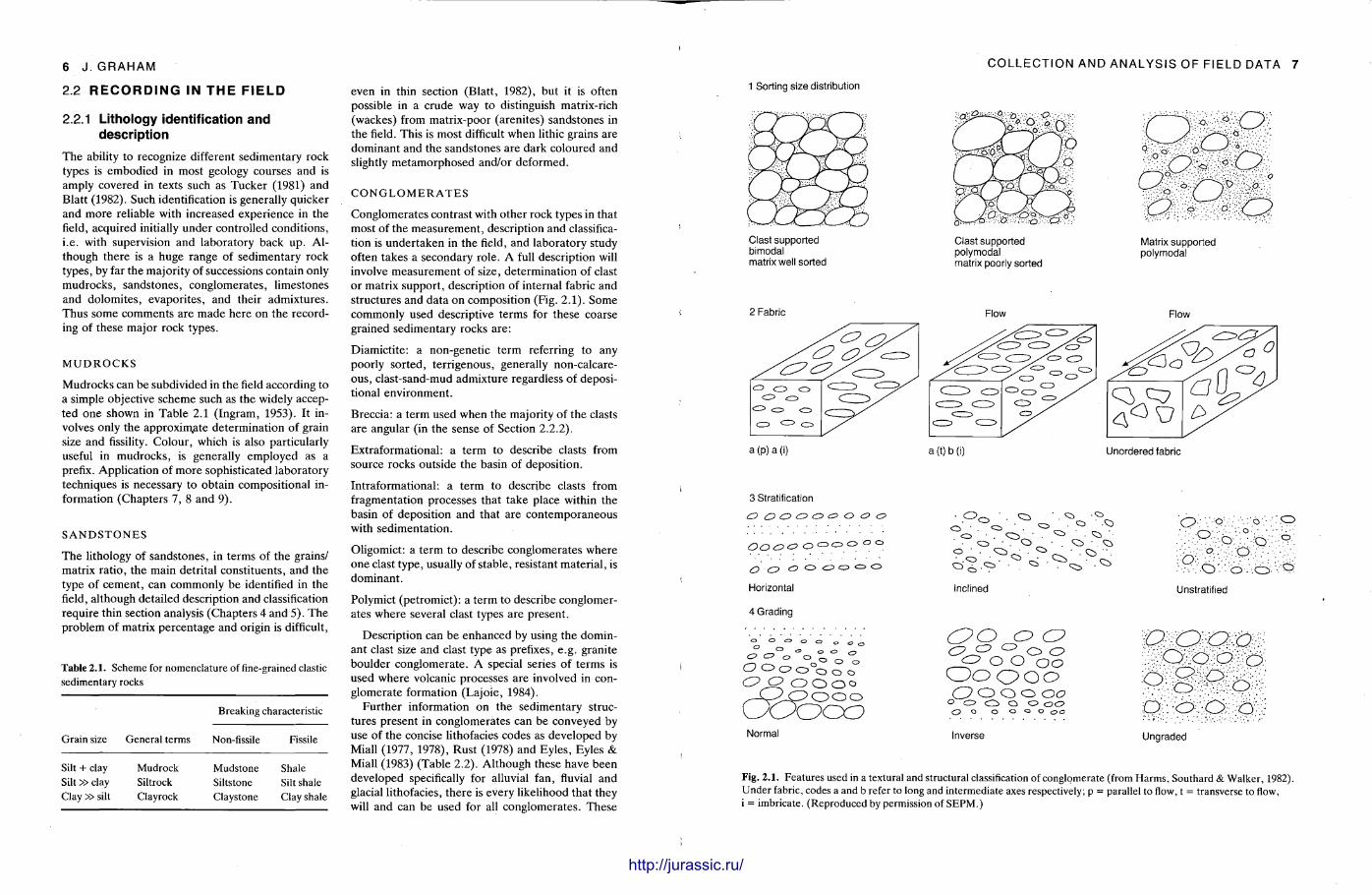
Conglomerates contrast with other rock types in that most of the measurement , description and classification is under taken in the field, and laboratory study often takes a secondary role. A full description will involve measurement of size, determinat ion of clast or matrix support , description of internal fabric and structures and data on composit ion (Fig. 2.1). Some commonly used descriptive terms for these coarse grained sedimentary rocks are:
Diamicti te: a non-genetic term referring to any poorly sorted, terr igenous, generally non-calcareous , clast-sand-mud admixture regardless of depositional environment .
Breccia: a term used when the majority of the clasts are angular (in the sense of Section 2.2.2).
Extraformational : a te rm to describe clasts from source rocks outside the basin of deposit ion.
Intraformational: a te rm to describe clasts from fragmentation processes that take place within the basin of deposition and that are contemporaneous with sedimentat ion.
Oligomict: a term to describe conglomerates where one clast type, usually of stable, resistant mater ia l , is dominant .
Polymict (petromict) : a te rm to describe conglomerates where several clast types are present .
Description can be enhanced by using the dominant clast size and clast type as prefixes, e.g. granite boulder conglomerate . A special series of terms is used where volcanic processes are involved in conglomerate formation (Lajoie, 1984).
Fur ther information on the sedimentary structures present in conglomerates can be conveyed by use of the concise lithofacies codes as developed by Miall (1977, 1978), Rust (1978) and Eyles, Eyles & Miall (1983) (Table 2.2). Al though these have been developed specifically for alluvial fan, fluvial and glacial lithofacies, there is every likelihood that they will and can be used for all conglomerates . These
IIIHIHIIHHHW
COLLECTION AND ANALYSIS OF FIELD DATA 7
1 Sorting size distribution
Clast supported Clast supported Matrix supported bimodal polymodal polymodal matrix well sorted matrix poorly sorted
2 Fabric Flow Flow
a (p) a (i) a (t) b (i) Unordered fabric
3 Stratification O O O O O C O £) O
OCxZ>& O
O <0 o o o o o o
Horizontal
4 Grading
° <=> o o 0 °
O O O o
Normal
Or
Inclined
C ? 0 o CD C o o
o o o o
O o o o o CD O o o ' o o O o O o ° o o o
O o . o CD
. ° Q. ° O ° . o a ; \ . ° • . . . O o . e > °
Unstratified
. : . 0 ' . 0 ' o ; o
Inverse Ungraded
Fig. 2.1. Features used in a textural and structural classification of conglomerate (from Harms, Southard & Walker, 1982). Under fabric, codes a and b refer to long and intermediate axes respectively; p = parallel to flow, t = transverse to flow, i = imbricate. (Reproduced by permission of SEPM.)
2 . 2 R E C O R D I N G IN T H E F I E L D
2.2 .1 Lithology identification and description
The ability to recognize different sedimentary rock types is embodied in most geology courses and is amply covered in texts such as Tucker (1981) and Blatt (1982). Such identification is generally quicker and more reliable with increased experience in the field, acquired initially under controlled condit ions, i .e. with supervision and laboratory back up . Although there is a huge range of sedimentary rock types, by far the majority of successions contain only mudrocks , sandstones, conglomerates , l imestones and dolomites , evapori tes , and their admixtures . Thus some comments are made here on the recording of these major rock types.
M U D R O C K S
Mudrocks can be subdivided in the field according to a simple objective scheme such as the widely accepted one shown in Table 2.1 ( Ingram, 1953). It involves only the approximate determinat ion of grain size and fissility. Colour , which is also particularly useful in mudrocks , is generally employed as a prefix. Application of more sophisticated laboratory techniques is necessary to obtain compositional information (Chapters 7, 8 and 9).
S A N D S T O N E S
The lithology of sandstones, in terms of the grains/ matrix rat io , the main detrital consti tuents, and the type of cement , can commonly be identified in the field, al though detailed description and classification require thin section analysis (Chapters 4 and 5). The problem of matrix percentage and origin is difficult,
http://jurassic.ru/

8 J . GRAHAM
(a) Criteria used for low sinuosity and glaciofluvial stream deposits (modified Table 2.2. Use of concise lithofacies from Miall, 1977) codes in field description
Code Lithofacies Sedimentary structures
Gms Massive, matrix- None supported gravel
Gm Massive or crudely Horizontal bedding, imbrication bedded gravel
Gt Gravel, stratified Trough crossbeds Gp Gravel, stratified Planar crossbeds St Sand, medium to Solitary (theta) or grouped (pi) trough
coarse, may be crossbeds pebbly
Sp Sand, medium to Solitary (alpha) or grouped (omicron) coarse, may be planar crossbeds pebbly
Sr Sand, very fine to Ripple marks of all types coarse
Sh Sand, very fine to very Horizontal lamination, parting or coarse, may be streaming lineation pebbly
SI Sand,fine Low angle (10°) crossbeds Se Erosional scours with Crude crossbedding
intraclasts Ss Sand, fine to coarse, Broad, shallow scours including eta
may be pebbly cross-stratification Sse, She, Spe Sand Analogous to Ss, Sh, Sp Fl Sand, silt, mud Fine lamination, very small ripples Fsc Silt, mud Laminated to massive Fcf Mud Massive with freshwater molluscs Fm Mud, silt Massive, dessication cracks Fr Silt, mud Rootlet traces C Coal, Carbonaceous Plants, mud films
mud P Carbonate Pedogenic features
(b) Diagnostic criteria for recognition of common matrix-supported diamict lithofacies (from Eyles et al., 1983)
Code Lithofacies Description
Dmm Matrix-supported, Structureless mud/sandVpebble massive admixture
Dmm(r) Dmm with evidence of Initially appears structureless but resedimentation careful cleaning, macro-sectioning, or
X-ray photography reveals subtle textural variability ahd fine structure (e.g. silt or clay stringers with small flow noses). Stratification less than 10% of unit thickness
COLLECTION AND ANALYSIS OF FIELD DATA 9
Code Lithofacies Sedimentary structures
Dmm(c) Dmm with evidence of Initially appears structureless but current reworking careful cleaning, macro-sectioning,
or textural analysis reveals fine structures and textural variability produced traction current activity (e.g. isolated ripples or ripple trains). Stratification less than 10% of unit thickness
Dmm(s) Matrix-rupported, Dense, matrix supported diamict with massive, sheared locally high clast concentrations.
Presence of distinctively shaped flat-iron clasts oriented parallel to flow direction, sheared
Dms Matrix-supported, Obvious textural differentiation or stratified diamict structure within diamict.
Stratification more than 10% of unit thickness
Dms(r) Dms with evidence of Flow noses frequently present; diamict resedimentation may contain rafts of deformed
silt/clay laminae and abundant silt/stringers and rip-up clasts. May show slight grading. Dms(r) units often have higher clast content than massive units; clast clusters common. Clast fabric random or parallel to bedding. Erosion and incorporation of underlying material may be evident
Dms(c) Dms with evidence of Diamict often coarse (winnowed) current reworking interbedded with sandy, silty and
gravelly beds showing evidence of traction current activity (e.g. ripples, trough or planar cross-bedding). May be recorded as Dmm, St, Dms, Sr etc. according to scale of logging. Abundant sandy stringers in diamict. Units may have channelized bases
Dmg Matrix-supported, Diamict exhibits variable vertical graded grading in either matrix or clast
content; may grade into Dcg Dmg(r) Dmg — with evidence Clast imbrication common
of resedimentation
schemes are still being refined and modified (cf. Eyles et al., 1983 with McCabe , Dardis & Hanvey, 1984 and Shultz, 1984) and the overlap between the
D (diamictite) and G (gravel) codes needs further clarification. T h e codes should not be regarded as all that is needed for environmental interpretation
http://jurassic.ru/
10 J . GRAHAM
(Dreimanis , 1984; Kemmis & Hallberg, 1984) but simply a concise and convenient shorthand description of some of the main observable features.
In addition to information on depositional processes and environments , polymict conglomerates can yield some information on the relative contribution of various source lithologies. However , there are many factors which affect the presence and size of clasts in conglomerates . The initial size of fragments released from the source area varies with lithology, being related to features such as bed thickness, joint spacing and resistance to weathering. In addition clasts have varying resistances to size reduction during transport . T o avoid spurious size-related effects, compositional data can be compared at constant size. This can be achieved either by counting the clast assemblage for a given size class or by a more detailed analysis in which the proportion of clast types is examined over a spectrum of size classes at a single site.
To determine the distribution of clast types by size, an area of several square metres should be chosen on a clean exposure surface on which all clasts can be identified easily. Areas of strong shape selection, common in some proximal fluvial and beach environments , should be avoided since this can introduce a bias towards anisotropic clast lithologies. Preliminary observations and the nature of the study will determine the number of lithological types to which clasts are assigned. Often crude discriminants, e.g. granite porphyry, e tc . , will suffice. More detailed studies require more subtle subdivision and may involve thin section checks on field identification.
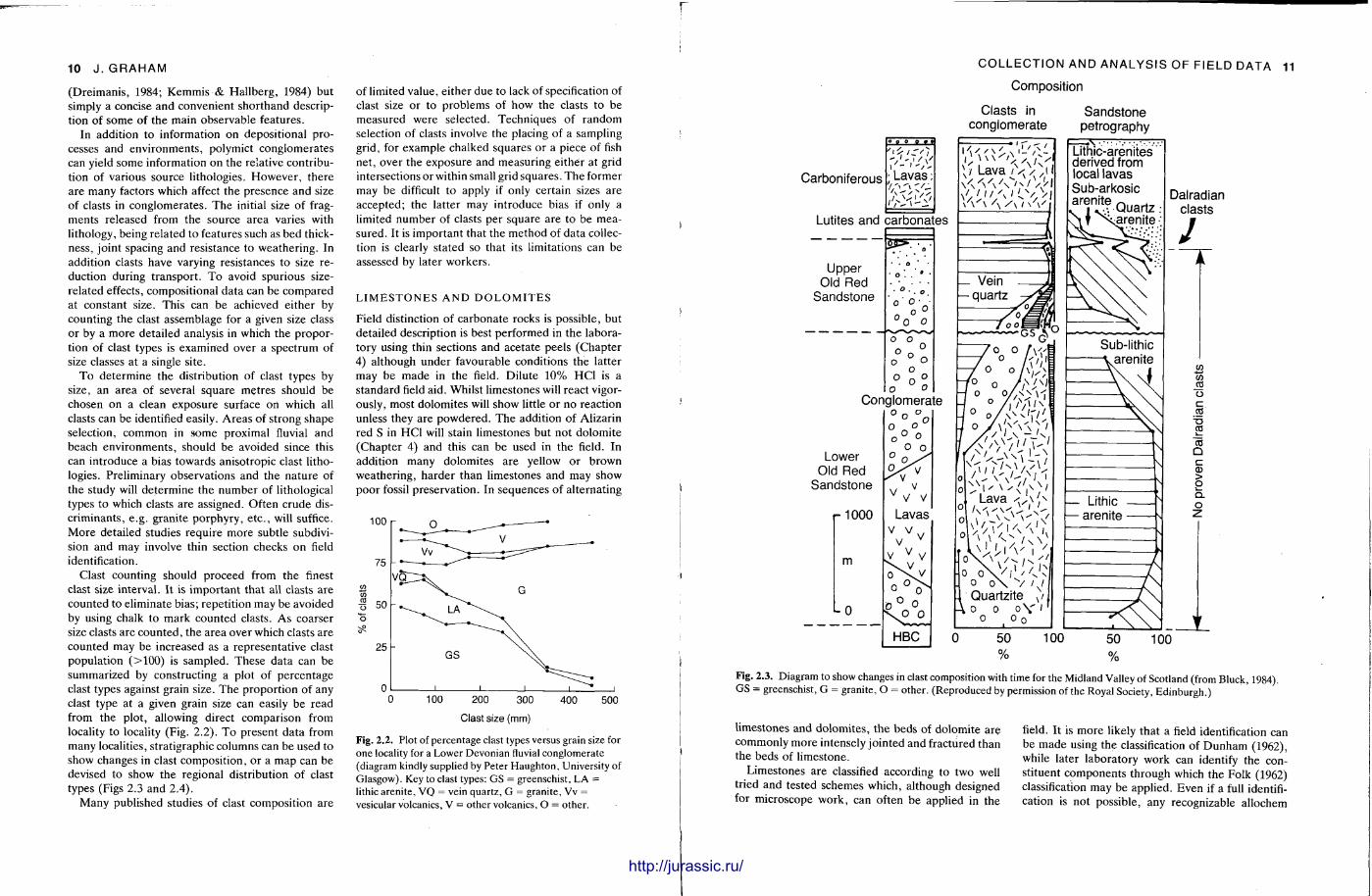
Clast counting should proceed from the finest clast size interval. It is important that all clasts are counted to eliminate bias; repetit ion may be avoided by using chalk to mark counted clasts. As coarser size clasts are counted, the area over which clasts are counted may be increased as a representat ive clast populat ion (>100) is sampled. These data can be summarized by constructing a plot of percentage clast types against grain size. The proport ion of any clast type at a given grain size can easily be read from the plot, allowing direct comparison from locality to locality (Fig. 2.2). To present data from many localities, stratigraphic columns can be used to show changes in clast composit ion, or a map can be devised to show the regional distribution of clast types (Figs 2.3 and 2.4).
Many published studies of clast composition are
of limited value, either due to lack of specification of clast size or to problems of how the clasts to be measured were selected. Techniques of random selection of clasts involve the placing of a sampling grid, for example chalked squares or a piece of fish net, over the exposure and measuring either at grid intersections or within small grid squares. The former may be difficult to apply if only certain sizes are accepted; the latter may introduce bias if only a limited number of clasts per square are to be measured. It is important that the method of data collection is clearly stated so that its limitations can be assessed by later workers .
L I M E S T O N E S A N D D O L O M I T E S
Field distinction of carbonate rocks is possible, but detailed description is best performed in the laboratory using thin sections and acetate peels (Chapter 4) although under favourable conditions the latter may be made in the field. Dilute 10% HC1 is a standard field aid. Whilst l imestones will react vigorously, most dolomites will show little or no reaction unless they are powdered . The addition of Alizarin red S in HC1 will stain limestones but not dolomite (Chapter 4) and this can be used in the field. In addition many dolomites are yellow or brown weathering, harder than limestones and may show poor fossil preservation. In sequences of alternating
0 100 200 300 400 500
Clast size (mm)
Fig. 2.2. Plot of percentage clast types versus grain size for one locality for a Lower Devonian fluvial conglomerate (diagram kindly supplied by Peter Haughton, University of Glasgow). Key to clast types: GS = greenschist, LA = lithic arenite, VQ = vein quartz, G = granite, Vv = vesicular volcanics, V = other volcanics, O = other.
Carboniferous • Lavas;
Lutites and carbonates
COLLECTION AND ANALYSIS OF FIELD DATA 11
Composition
Clasts in conglomerate
Sandstone petrography
\ / Lava /V/>l|
, Lava s \ ' \
\ ^ i V i ' O V X / ^ si
Lithic-arenites derived from local lavas Sub-arkosic ^ Q u a r t z
f xa ren i te
Sub-lithic .arenite
— Lithic — arenite
100
Dalradian clasts
w GO m o c « CO "co Q c CD > O i Q_ O
100 Fig. 2.3. Diagram to show changes in clast composition with time for the Midland Valley of Scotland (from Bluck, 1984). GS = greenschist, G = granite, O = other. (Reproduced by permission of the Royal Society, Edinburgh.)
l imestones and dolomites , the beds of dolomite are commonly more intensely jointed and fractured than the beds of l imestone.
Limestones are classified according to two well tried and tested schemes which, although designed for microscope work, can often be applied in the
field. It is more likely that a field identification can be made using the classification of Dunham (1962), while later laboratory work can identify the constituent components through which the Folk (1962) classification may be applied. Even if a full identification is not possible, any recognizable allochem
http://jurassic.ru/
1 2 J . GRAHAM
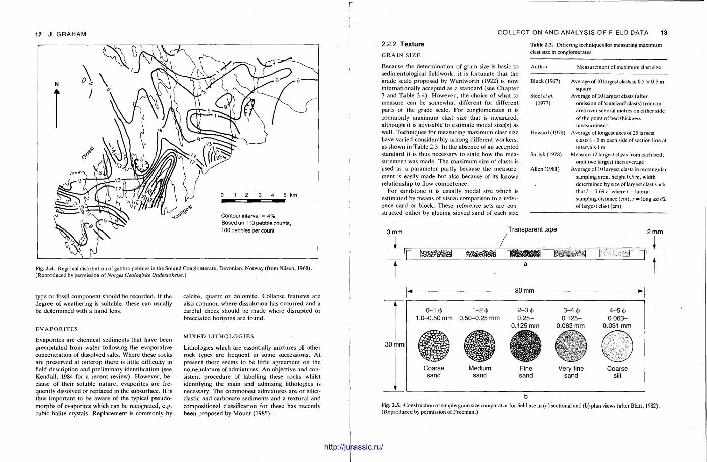
5 km
Contour interval = 4% Based on 110 pebble counts, 100 pebbles per count
Fig. 2.4. Regional distribution of gabbro pebbles in the Solund Conglomerate, Devonian, Norway (from Nilsen, 1968). (Reproduced by permission of Norges Geologiske Undersokelse.)
type or fossil component should be recorded. If the degree of weather ing is suitable, these can usually be determined with a hand lens.
E V A P O R I T E S
Evapori tes are chemical sediments that have been precipitated from water following the evaporative concentrat ion of dissolved salts. Where these rocks are preserved at outcrop there is little difficulty in field description and preliminary identification (see Kendall , 1984 for a recent review). However , because of their soluble na ture , evaporites are frequently dissolved or replaced in the subsurface. It is thus important to be aware of the typical pseudo-morphs of evaporites which can be recognized, e.g. cubic halite crystals. Replacement is commonly by
calcite, quartz or dolomite . Collapse features are also common where dissolution has occurred and a careful check should be made where disrupted or brecciated horizons are found.
M I X E D L I T H O L O G I E S
Lithologies which are essentially mixtures of o ther rock types are frequent in some successions. A t present there seems to be little agreement on the nomenclature of admixtures. A n objective and consistent procedure of labelling these rocks whilst identifying the main and admixing lithologies is necessary. The commonest admixtures are of silici-clastic and carbonate sediments and a textural and compositional classification for these has recently been proposed by Mount (1985).
COLLECTION AND ANALYSIS OF FIELD DATA 13
2.2.2 Texture
G R A I N S I Z E
Because the determinat ion of grain size is basic to sedimentological fieldwork, it is fortunate that the grade scale proposed by Wentwor th (1922) is now internationally accepted as a standard (see Chapter 3 and Table 3.4). However , the choice of what to measure can be somewhat different for different parts of the grade scale. For conglomerates it is commonly maximum clast size that is measured , although it is advisable" to est imate modal size(s) as well. Techniques for measuring maximum clast size have varied considerably among different workers , as shown in Table 2.3. In the absence of an accepted s tandard it is thus necessary to state how the measurement was made . The maximum size of clasts is used as a parameter partly because the measurement is easily made but also because of its known relationship to flow competence .
For sandstone it is usually modal size which is estimated by means of visual comparison to a reference card or block. These reference sets are constructed either by glueing sieved sand of each size
T a b l e 2.3. Differing techniques for measuring maximum clast size in conglomerates
Author Measurement of maximum clast size
Bluck (1967) Average of 10 largest clasts in 0.5 x 0.5 m square
Steel et al. Average of 10 largest clasts (after (1977) omission of 'outsized' clasts) from an
area over several metres on either side of the point of bed thickness measurement
Heward (1978) Average of longest axes of 25 largest clasts 1—5 m each side of section line at intervals 1 m
Surlyk (1978) Measure 12 largest clasts from each bed; omit two largest then average
Allen (1981) Average of 10 largest clasts in rectangular sampling area, height 0.5 m, width determined by size of largest clast such that / = 0.69 r2 where / = lateral sampling distance (cm), r = long axis/2 of largest clast (cm)
3 mm Transparent tape 2 mm
-80 mm-
0-1 <b
1.0-0.50 mm 1-2 cb
0.50-0.25 mm
30 mm
Coarse sand
Medium sand
2-3 <b 0.25-
0.125 mm
3-4 cb 4-5 <b
0.125- 0.063-0.063 mm 0.031 mm
Very fine Coarse sand silt
Fig. 2.5. Construction of simple grain size comparator for field use in (a) sectional and (b) plan views (after Blatt, 1982). (Reproduced by permission of Freeman.)
http://jurassic.ru/
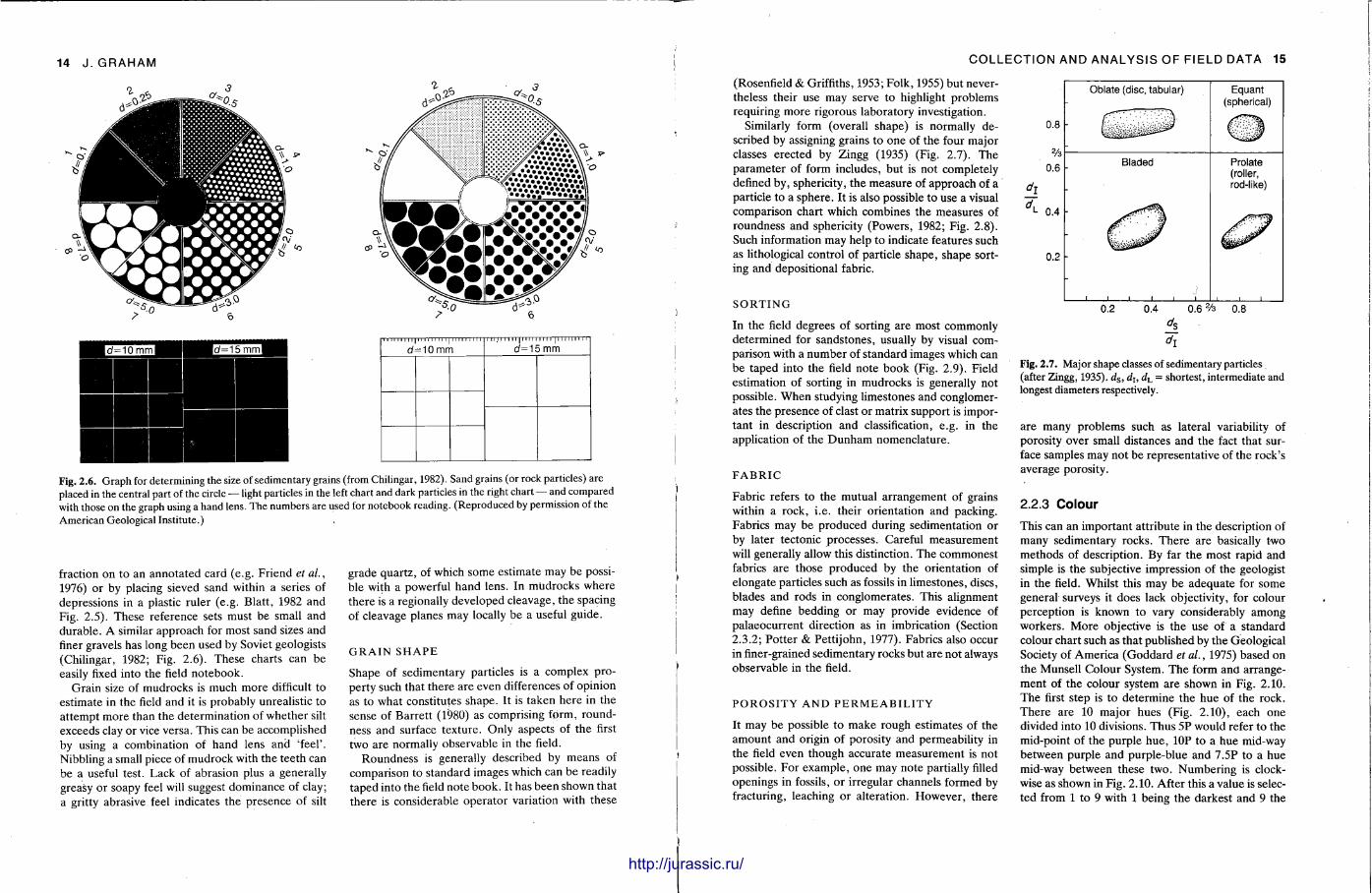
14 J .GRAHAM
Fig. 2.6. Graph for determining the size of sedimentary grains (from Chilingar, 1982). Sand grains (or rock particles) are placed in the central part of the circle — light particles in the left chart and dark particles in the right chart — and compared with those on the graph using a hand lens. The numbers are used for notebook reading. (Reproduced by permission of the American Geological Institute.)
fraction on to an annota ted card (e.g. Friend et al., 1976) or by placing sieved sand within a series of depressions in a plastic ruler (e.g. Blatt , 1982 and Fig. 2.5). These reference sets must be small and durable . A similar approach for most sand sizes and finer gravels has long been used by Soviet geologists (Chilingar, 1982; Fig. 2.6). These charts can be easily fixed into the field notebook.
Grain size of mudrocks is much more difficult to est imate in the field and it is probably unrealistic to a t tempt more than the determinat ion of whether silt exceeds clay or vice versa. This can be accomplished by using a combination of hand lens and 'feel ' . Nibbling a small piece of mudrock with the teeth can be a useful test. Lack of abrasion plus a generally greasy or soapy feel will suggest dominance of clay; a gritty abrasive feel indicates the presence of silt
grade quar tz , of which some est imate may be possible with a powerful hand lens. In mudrocks where there is a regionally developed cleavage, the spacing of cleavage planes may locally be a useful guide.
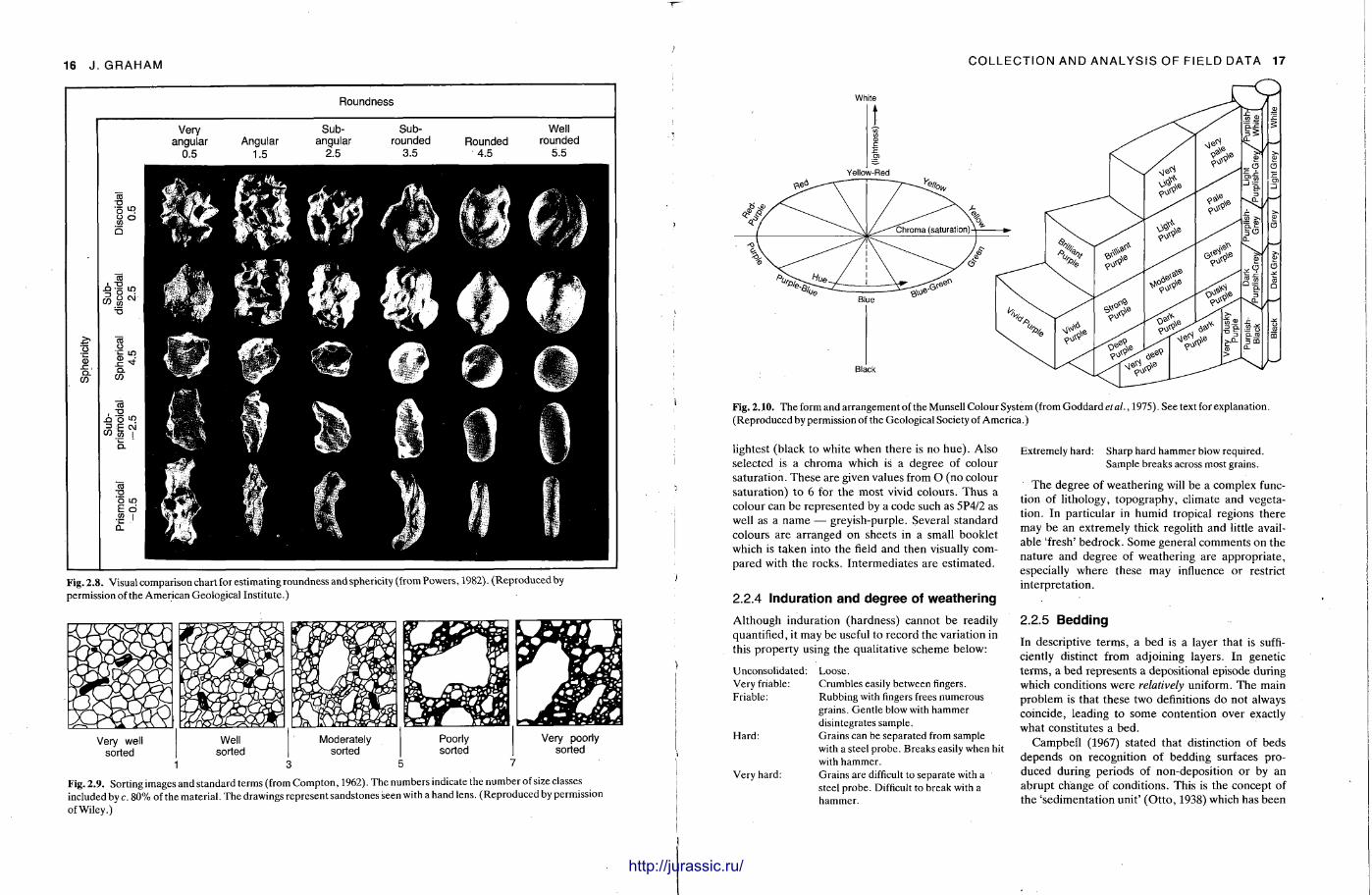
G R A I N S H A P E
Shape of sedimentary particles is a complex property such that there are even differences of opinion as to what constitutes shape. It is taken here in the sense of Barret t (1980) as comprising form, roundness and surface texture . Only aspects of the first two are normally observable in the field.
Roundness is generally described by means of comparison to s tandard images which can be readily taped into the field note book. It has been shown that there is considerable operator variation with these
f f f * + I
COLLECTION AND ANALYSIS OF FIELD DATA 15
(Rosenfield & Griffiths, 1953; Folk, 1955) but nevertheless their use may serve to highlight problems requiring more rigorous laboratory investigation.
Similarly form (overall shape) is normally described by assigning grains to one of the four major classes erected by Zingg (1935) (Fig. 2.7). The parameter of form includes, but is not completely defined by, sphericity, the measure of approach of a particle to a sphere . It is also possible to use a visual comparison chart which combines the measures of roundness and sphericity (Powers, 1982; Fig. 2.8). Such information may help to indicate features such as lithological control of particle shape, shape sorting and depositional fabric.
S O R T I N G
In the field degrees of sorting are most commonly determined for sandstones, usually by visual comparison with a number of s tandard images which can be taped into the field note book (Fig. 2.9). Field estimation of sorting in mudrocks is generally not possible. W h e n studying limestones and conglomerates the presence of clast or matrix support is important in description and classification, e.g. in the application of the D u n h a m nomenclature .
F A B R I C
Fabric refers to the mutual arrangement of grains within a rock, i.e. their orientation and packing. Fabrics may be produced during sedimentation or by later tectonic processes. Careful measurement will generally allow this distinction. The commonest fabrics are those produced by the orientation of elongate particles such as fossils in l imestones, discs, blades and rods in conglomerates. This alignment may define bedding or may provide evidence of palaeocurrent direction as in imbrication (Section 2.3.2; Pot ter & Pet t i john, 1977). Fabrics also occur in finer-grained sedimentary rocks but are not always observable in the field.
P O R O S I T Y A N D P E R M E A B I L I T Y
It may be possible to make rough estimates of the amount and origin of porosity and permeability in the field even though accurate measurement is not possible. For example , one may note partially filled openings in fossils, or irregular channels formed by fracturing, leaching or alteration. However , there
0.2
Oblate (disc, tabular) Equant (spherical)
Bladed
~i
Prolate (roller, rod-like)
i i i _ l I I I I l_l L_ 0.2 0.4 0.6 % 0.8
Cfs di
Fig. 2.7. Major shape classes of sedimentary particles _ (after Zingg, 1935). ds, a\, d L = shortest, intermediate and longest diameters respectively.
are many problems such as lateral variability of porosity over small distances and the fact that surface samples may not be representat ive of the rock's average porosity.
2.2.3 Colour
This can an important at tr ibute in the description of many sedimentary rocks. There are basically two methods of description. By far the most rapid and simple is the subjective impression of the geologist in the field. Whilst this may be adequate for some general surveys it does lack objectivity, for colour perception is known to vary considerably among workers . More objective is the use of a s tandard colour chart such as that published by the Geological Society of Amer ica (Goddard et al., 1975) based on the Munsell Colour System. The form and arrangement of the colour system are shown in Fig. 2.10. The first s tep is to determine the hue of the rock. There are 10 major hues (Fig. 2.10), each one divided into 10 divisions. Thus 5P would refer to the mid-point of the purple hue , 10P to a hue mid-way between purple and purple-blue and 7.5P to a hue mid-way between these two. Number ing is clockwise as shown in Fig. 2.10. After this a value is selected from 1 to 9 with 1 being the darkest and 9 the
http://jurassic.ru/
16 J . GRAHAM
Very well sorted
Well sorted
Moderately sorted
Poorly sorted
Very poorly sorted
1 7
Fig. 2.9. Sorting images and standard terms (from Compton, 1962). The numbers indicate the number of size classes included by c. 80% of the material. The drawings represent sandstones seen with a hand lens. (Reproduced by permission ofWiley.)
COLLECTION AND ANALYSIS OF FIELD DATA 17
Fig. 2.10. The form and arrangement of the Munsell Colour System (from Goddard et al., 1975). See text for explanation. (Reproduced by permission of the Geological Society of America.)
lightest (black to white when there is no hue) . Also selected is a chroma which is a degree of colour saturat ion. These are given values from O (no colour saturat ion) to 6 for the most vivid colours. Thus a colour can be represented by a code such as 5P4/2 as well as a name — greyish-purple. Several standard colours are arranged on sheets in a small booklet which is taken into the field and then visually compared with the rocks. Intermediates are est imated.
2.2.4 Induration and degree of weathering
Although induration (hardness) cannot be readily quantified, it may be useful to record the variation in this property using the qualitative scheme below:
Unconsolidated: Loose. Very friable: Crumbles easily between fingers. Friable: Rubbing with fingers frees numerous
grains. Gentle blow with hammer disintegrates sample.
Hard: Grains can be separated from sample with a steel probe. Breaks easily when hit with hammer.
Very hard: Grains are difficult to separate with a steel probe. Difficult to break with a hammer.
Extremely hard: Sharp hard hammer blow required. Sample breaks across most grains.
T h e degree of weathering will be a complex function of lithology, topography, climate and vegetation. In particular in humid tropical regions there may be an extremely thick regolith and little available 'fresh' bedrock. Some general comments on the na ture and degree of weather ing are appropr ia te , especially where these may influence or restrict interpretat ion.
2.2.5 Bedding
In descriptive te rms , a bed is a layer that is sufficiently distinct from adjoining layers. In genetic terms, a bed represents a depositional episode during which conditions were relatively uniform. The main problem is that these two definitions do not always coincide, leading to some content ion over exactly what constitutes a bed.
Campbell (1967) stated that distinction of beds depends on recognition of bedding surfaces produced during periods of non-deposit ion or by an abrupt change of condit ions. This is the concept of the 'sedimentat ion unit ' (Ot to , 1938) which has been
http://jurassic.ru/
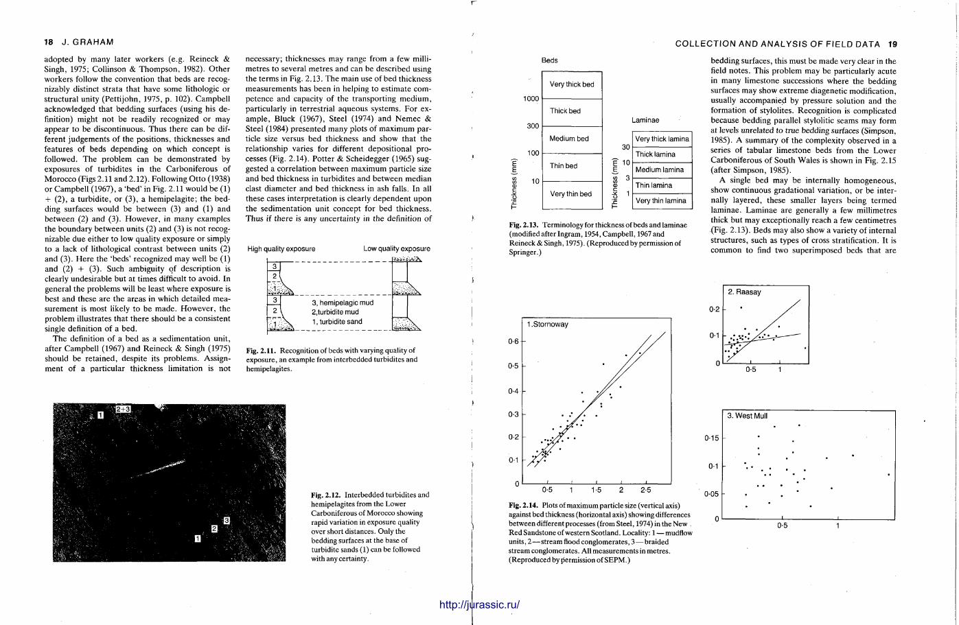
18 J . GRAHAM
adopted by many later workers (e.g. Reineck & Singh, 1975; Collinson & Thompson , 1982). O the r workers follow the convention that beds are recognizably distinct strata that have some lithologic or structural unity (Pett i john, 1975, p . 102). Campbell acknowledged that bedding surfaces (using his definition) might not be readily recognized or may appear to be discontinuous. Thus there can be different judgements of the positions, thicknesses and features of beds depending on which concept is followed. The problem can be demonst ra ted by exposures of turbidites in the Carboniferous of Morocco (Figs 2.11 and 2.12). Following Ot to (1938) or Campbell (1967), a 'bed ' in Fig. 2.11 would be (1) + (2), a turbidite, or (3) , a hemipelagite; the bedding surfaces would be between (3) and (1) and between (2) and (3). However , in many examples the boundary between units (2) and (3) is not recognizable due either to low quality exposure or simply to a lack of lithological contrast between units (2) and (3). He re the 'beds ' recognized may well be (1) and (2) + (3). Such ambiguity of description is clearly undesirable but at times difficult to avoid. In general the problems will be least where exposure is best and these are the areas in which detailed measurement is most likely to be made . However , the problem illustrates that there should be a consistent single definition of a bed.
The definition of a bed as a sedimentat ion unit , after Campbell (1967) and Reineck & Singh (1975) should be retained, despite its problems. Assignment of a particular thickness limitation is not
necessary; thicknesses may range from a few millimetres to several metres and can be described using the terms in Fig. 2.13. The main use of bed thickness measurements has been in helping to est imate competence and capacity of the transport ing medium, particularly in terrestrial aqueous systems. For example , Bluck (1967), Steel (1974) and Nemec & Steel (1984) presented many plots of maximum particle size versus bed thickness and show that the relationship varies for different depositional processes (Fig. 2.14). Pot ter & Scheidegger (1965) suggested a correlation between maximum particle size and bed thickness in turbidites and between median clast diameter and bed thickness in ash falls. In all these cases interpretat ion is clearly dependent upon the sedimentat ion unit concept for bed thickness. Thus if there is any uncertainty in the definition of
High quality exposure Low quality exposure
Ico L_
2 I
3 3, h e m i p e l a g i c m u d 2 I 2 ,turbidite m u d
1 \ . 1, turbidite s a n d
Fig. 2.11. Recognition of beds with varying quality of exposure, an example from interbedded turbidites and hemipelagites.
Fig. 2.12. Interbedded turbidites and hemipelagites from the Lower Carboniferous of Morocco showing rapid variation in exposure quality over short distances. Only the bedding surfaces at the base of turbidite sands (1) can be followed with any certainty.
COLLECTION AND ANALYSIS OF FIELD DATA 19
Beds
1000
300
100
10
Very thick bed
Thick bed
Medium bed
Thin bed
Very thin bed
Laminae
30
If 10 E v> 3 m CO * 1
Very thick l a m i n a
Thick lamina
Medium lamina
Thin lamina
Very thin l a m i n a
Fig. 2.13. Terminology for thickness of beds and laminae (modified after Ingram, 1954, Campbell, 1967 and Reineck & Singh, 1975). (Reproduced by permission of Springer.)
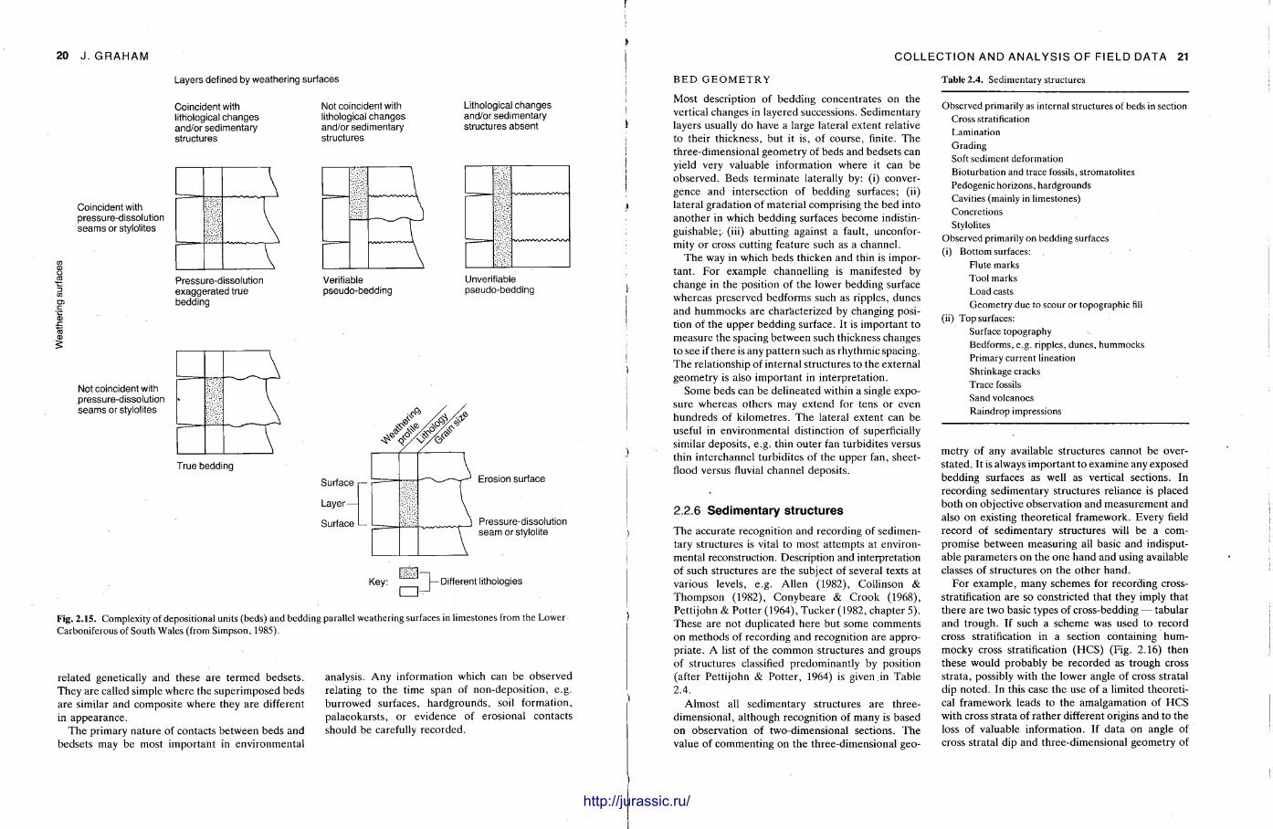
bedding surfaces, this must be made very clear in the field notes. This problem may be particularly acute in many limestone successions where the bedding surfaces may show extreme diagenetic modification, usually accompanied by pressure solution and the formation of stylolites. Recognit ion is complicated because bedding parallel stylolitic seams may form at levels unrelated to true bedding surfaces (Simpson, 1985). A summary of the complexity observed in a series of tabular l imestone beds from the Lower Carboniferous of South Wales is shown in Fig. 2.15 (after Simpson, 1985).
A single bed may be internally homogeneous , show continuous gradational variation, or be internally layered, these smaller layers being termed laminae. Laminae are generally a few millimetres thick but may exceptionally reach a few centimetres (Fig. 2.13). Beds may also show a variety of internal structures, such as types of cross stratification. It is common to find two superimposed beds that are
Fig. 2.14. Plots of maximum particle size (vertical axis) against bed thickness (horizontal axis) showing differences between different processes (from Steel, 1974) in the New . Red Sandstone of western Scotland. Locality: 1 — mudflow units, 2—stream flood conglomerates, 3 — braided stream conglomerates. All measurements in metres. (Reproduced by permission of SEPM.)
0-5 1
0-15
0-1 h
0-05
0
3. West Mull
0-5
http://jurassic.ru/
20 J. GRAHAM
Layers defined by weathering surfaces
Coincident with lithological changes and/or sedimentary structures
Not coincident with lithological changes and/or sedimentary structures
Lithological changes and/or sedimentary structures absent
Different lithologies
Fig. 2.15. Complexity of depositional units (beds) and bedding parallel weathering surfaces in limestones from the Lower Carboniferous of South Wales (from Simpson, 1985).
related genetically and these are te rmed bedsets . They are called simple where the superimposed beds are similar and composite where they are different in appearance.
The primary nature of contacts between beds and bedsets may be most important in environmental
analysis. Any information which can be observed relating to the t ime span of non-deposit ion, e.g. burrowed surfaces, hardgrounds , soil formation, palaeokarsts , or evidence of erosional contacts should be carefully recorded.
COLLECTION AND ANALYSIS OF FIELD DATA 21
B E D G E O M E T R Y
Most description of bedding concentrates on the vertical changes in layered successions. Sedimentary layers usually do have a large lateral extent relative to their thickness, but it is, of course, finite. The three-dimensional geometry of beds and bedsets can yield very valuable information where it can be observed. Beds terminate laterally by: (i) convergence and intersection of bedding surfaces; (ii) lateral gradation of material comprising the bed into another in which bedding surfaces become indistinguishable; (iii) abutt ing against a fault, unconformity or cross cutting feature such as a channel .
The way in which beds thicken and thin is important . For example channelling is manifested by change in the position of the lower bedding surface whereas preserved bedforms such as ripples, dunes and hummocks are characterized by changing position of the upper bedding surface. It is important to measure the spacing between such thickness changes to see if there is any pat tern such as rhythmic spacing. The relationship of internal structures to the external geometry is also important in interpretat ion.
Some beds can be delineated within a single exposure whereas others may extend for tens or even hundreds of kilometres. The lateral extent can be useful in environmental distinction of superficially similar deposits , e.g. thin outer fan turbidites versus thin interchannel turbidites of the upper fan, sheet-flood versus fluvial channel deposits .
2.2.6 Sedimentary structures
The accurate recognition and recording of sedimentary structures is vital to most a t tempts at environmental reconstruction. Description and interpretation of such structures are the subject of several texts at various levels, e.g. Allen (1982), Collinson & Thompson (1982), Conybeare & Crook (1968), Petti john & Pot ter (1964), Tucker (1982, chapter 5). These are not duplicated here but some comments on methods of recording and recognition are appropr ia te . A list of the common structures and groups of structures classified predominantly by position (after Pettijohn & Pot ter , 1964) is given in Table 2.4.
Almost all sedimentary structures are three-dimensional , al though recognition of many is based on observation of two-dimensional sections. The value of commenting on the three-dimensional geo-
Table 2.4. Sedimentary structures
Observed primarily as internal structures of beds in section Cross stratification Lamination Grading Soft sediment deformation Bioturbation and trace fossils, stromatolites Pedogenic horizons, hardgrounds Cavities (mainly in limestones) Concretions Stylolites
Observed primarily on bedding surfaces (i) Bottom surfaces:
Flute marks Tool marks Load casts Geometry due to scour or topographic fill
(ii) Top surfaces: Surface topography Bedforms, e.g. ripples, dunes, hummocks Primary current lineation Shrinkage cracks Trace fossils Sand volcanoes Raindrop impressions
metry of any available structures cannot be overstated. It is always important to examine any exposed bedding surfaces as well as vertical sections. In recording sedimentary structures reliance is placed both on objective observation and measurement and also on existing theoretical framework. Every field record of sedimentary structures will be a compromise between measuring all basic and indisputable parameters on the one hand and using available classes of structures on the other hand.
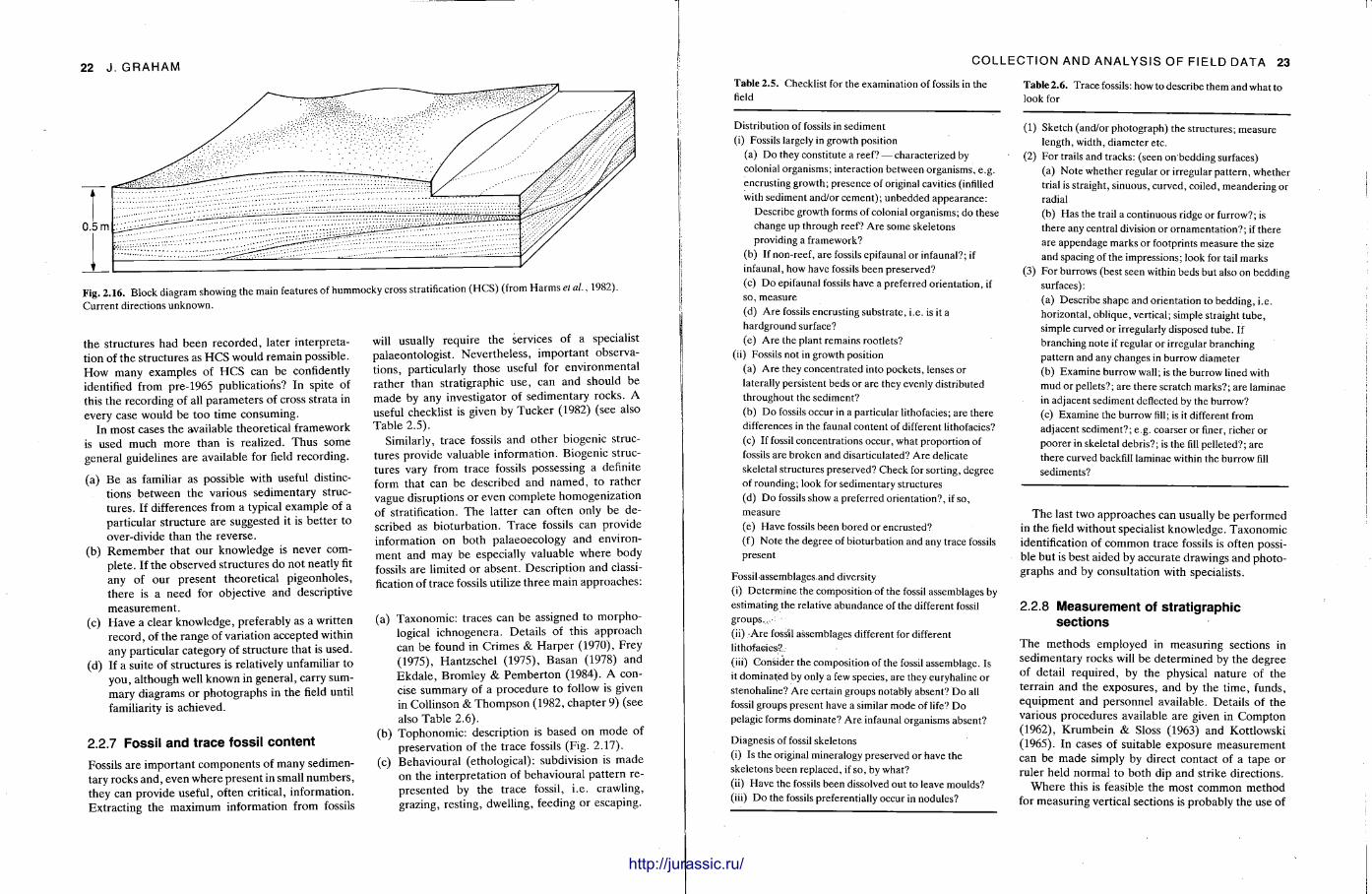
For example , many schemes for recording cross-stratification are so constricted that they imply that there are two basic types of cross-bedding — tabular and t rough. If such a scheme was used to record cross stratification in a section containing hum-mocky cross stratification (HCS) (Fig. 2.16) then these would probably be recorded as t rough cross strata, possibly with the lower angle of cross stratal dip noted. In this case the use of a limited theoretical framework leads to the amalgamation of H C S with cross strata of ra ther different origins and to the loss of valuable information. If data on angle of cross stratal dip and three-dimensional geometry of
"HIIII! http://jurassic.ru/
22 J . GRAHAM
0.5 m
Fig. 2.16. Block diagram showing the main features of hummocky cross stratification (HCS) (from Harms et al., 1982). Current directions unknown.
the structures had been recorded, later interpretation of the structures as H C S would remain possible. How many examples of H C S can be confidently identified from pre-1965 publications? In spite of this the recording of all parameters of cross strata in every case would be too t ime consuming.
In most cases the available theoretical framework is used much more than is realized. Thus some general guidelines are available for field recording.
(a) Be as familiar as possible with useful distinctions between the various sedimentary structures . If differences from a typical example of a particular structure are suggested it is bet ter to over-divide than the reverse.
(b) R e m e m b e r that our knowledge is never complete. If the observed structures do not neatly fit any of our present theoretical pigeonholes, there is a need for objective and descriptive measurement .
(c) Have a clear knowledge, preferably as a written record, of the range of variation accepted within any particular category of structure that is used.
(d) If a suite of structures is relatively unfamiliar to you, although well known in general , carry summary diagrams or photographs in the field until familiarity is achieved.
2.2.7 Fossil and trace fossil content
Fossils are important components of many sedimentary rocks and, even where present in small numbers , they can provide useful, often critical, information. Extracting the maximum information from fossils
will usually require the services of a specialist palaeontologist . Nevertheless, important observations, particularly those useful for environmental rather than stratigraphic use, can and should be made by any investigator of sedimentary rocks. A useful checklist is given by Tucker (1982) (see also Table 2.5).
Similarly, t race fossils and other biogenic structures provide valuable information. Biogenic structures vary from trace fossils possessing a definite form that can be described and named , to ra ther vague disruptions or even complete homogenizat ion of stratification. The latter can often only be described as bioturbat ion. Trace fossils can provide information on both palaeoecology and environment and may be especially valuable where body fossils are limited or absent . Descript ion and classification of trace fossils utilize three main approaches:
(a) Taxonomic: traces can be assigned to morphological ichnogenera. Details of this approach can be found in Crimes & Harpe r (1970), Frey (1975), Hantzschel (1975), Basan (1978) and Ekda l e , Bromley & Pember ton (1984). A concise summary of a procedure to follow is given in Collinson & Thompson (1982, chapter 9) (see also Table 2.6).
(b) Tophonomic : description is based on mode of preservation of the trace fossils (Fig. 2.17).
(c) Behavioural (ethological): subdivision is made on the interpretat ion of behavioural pa t tern represented by the trace fossil, i .e. crawling, grazing, resting, dwelling, feeding or escaping.
COLLECTION AND ANALYSIS OF FIELD DATA 2 3
Table 2.5. Checklist for the examination of fossils in the field
Distribution of fossils in sediment (i) Fossils largely in growth position
(a) Do they constitute a reef? — characterized by colonial organisms; interaction between organisms, e.g. encrusting growth; presence of original cavities (infilled with sediment and/or cement); unbedded appearance:
Describe growth forms of colonial organisms; do these change up through reef? Are some skeletons providing a framework?
(b) If non-reef, are fossils epifaunal or infaunal?; if infaunal, how have fossils been preserved? (c) Do epifaunal fossils have a preferred orientation, if so, measure (d) Are fossils encrusting substrate, i.e. is it a hardground surface? (e) Are the plant remains rootlets?
(ii) Fossils not in growth position (a) Are they concentrated into pockets, lenses or laterally persistent beds or are they evenly distributed throughout the sediment? (b) Do fossils occur in a particular lithofacies; are there differences in the faunal content of different lithofacies? (c) If fossil concentrations occur, what proportion of fossils are broken and disarticulated? Are delicate skeletal structures preserved? Check for sorting, degree of rounding; look for sedimentary structures (d) Do fossils show a preferred orientation?, if so, measure (e) Have fossils been bored or encrusted? (f) Note the degree of bioturbation and any trace fossils present
Fossil assemblagesand diversity (i) Determine the composition of the fossil assemblages by estimating the relative abundance of the different fossil groups. (ii) Are fossil assemblages different for different lithofacies?. (iii) Consider the composition of the fossil assemblage. Is it dominated by only a few species, are they euryhaline or stenohaline? Are certain groups notably absent? Do all fossil groups present have a similar mode of life? Do pelagic forms dominate? Are infaunal organisms absent?
Diagnesis of fossil skeletons (i) Is the original mineralogy preserved or have the skeletons been replaced, if so, by what? (ii) Have the fossils been dissolved out to leave moulds? (iii) Do the fossils preferentially occur in nodules?
Table 2.6. Trace fossils: how to describe them and what to look for
(1) Sketch (and/or photograph) the structures; measure length, width, diameter etc.
(2) For trails and tracks: (seen on bedding surfaces) (a) Note whether regular or irregular pattern, whether trial is straight, sinuous, curved, coiled, meandering or radial (b) Has the trail a continuous ridge or furrow?; is there any central division or ornamentation?; if there are appendage marks or footprints measure the size and spacing of the impressions; look for tail marks
(3) For burrows (best seen within beds but also on bedding surfaces): (a) Describe shape and orientation to bedding, i.e. horizontal, oblique, vertical; simple straight tube, simple curved or irregularly disposed tube. If branching note if regular or irregular branching pattern and any changes in burrow diameter (b) Examine burrow wall; is the burrow lined with mud or pellets?; are there scratch marks?; are laminae in adjacent sediment deflected by the burrow? (c) Examine the burrow fill; is it different from adjacent sediment?; e.g. coarser or finer, richer or poorer in skeletal debris?; is the fill pelleted?; are there curved backfill laminae within the burrow fill sediments?
The last two approaches can usually be performed in the field without specialist knowledge. Taxonomic identification of common trace fossils is often possible but is best aided by accurate drawings and photographs and by consultation with specialists.
2.2.8 Measurement of stratigraphic sections
The methods employed in measuring sections in sedimentary rocks will be determined by the degree of detail required, by the physical nature of the terrain and the exposures, and by the t ime, funds, equipment and personnel available. Details of the various procedures available are given in Compton (1962), Krumbein & Sloss (1963) and Kottlowski (1965). In cases of suitable exposure measurement can be made simply by direct contact of a tape or ruler held normal to both dip and strike directions.
Where this is feasible the most common method for measuring vertical sections is probably the use of
"'lllll http://jurassic.ru/
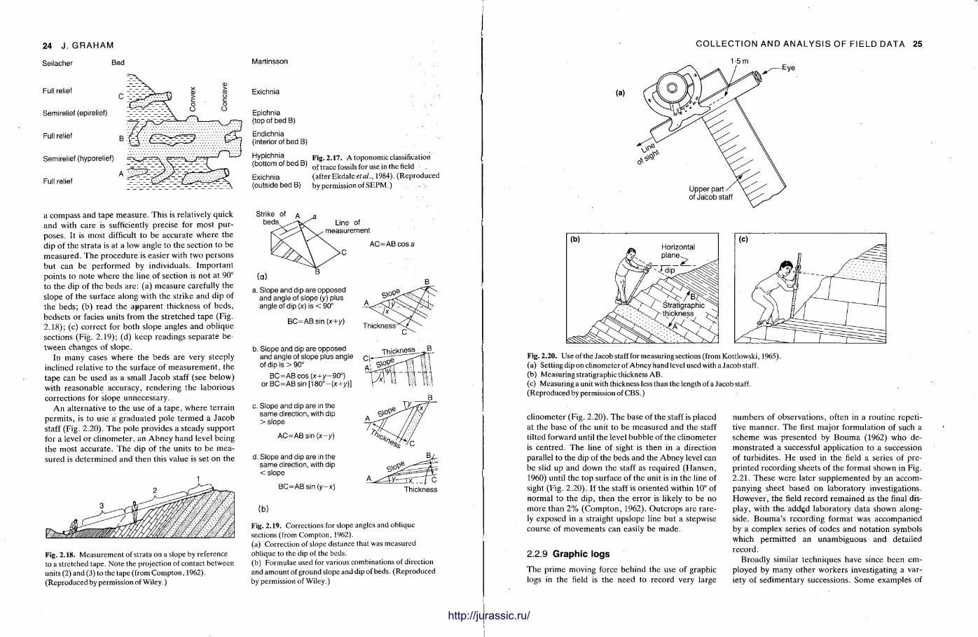
24 J. GRAHAM
Martinsson
Exichnia
Epichnia (top of bed B)
Endichnia (interior of bed B)
Hypichnia Fig. 2.17. A toponomic classification (bottom of bed B) rftrac£ fossils for u s e j n t h e field
Exichnia (afterEkdaleefa/., 1984). (Reproduced (outside bed B) by permission of SEPM.)
a compass and tape measure . This is relatively quick and with care is sufficiently precise for most purposes. It is most difficult to be accurate where the dip of the strata is at a low angle to the section to be measured. The procedure is easier with two persons but can be performed by individuals. Impor tant points to note where the line of section is not at 90° to the dip of the beds are: (a) measure carefully the slope of the surface along with the strike and dip of the beds; (b) read the apparent thickness of beds, bedsets or facies units from the stretched tape (Fig. 2.18); (c) correct for both slope angles and oblique sections (Fig. 2.19); (d) keep readings separate between changes of slope.
In many cases where the beds are very steeply inclined relative to the surface of measurement , the tape can be used as a small Jacob staff (see below) with reasonable accuracy, rendering the laborious corrections for slope unnecessary.
A n alternative to the use of a tape, where terrain permits , is to use a graduated pole te rmed a Jacob staff (Fig. 2.20). T h e pole provides a steady suppor t for a level or cl inometer, an Abney hand level being the most accurate. The dip of the units to be measured is determined and then this value is set on the
Strike of beds
Fig. 2.18. Measurement of strata on a slope by reference to a stretched tape. Note the projection of contact between units (2) and (3) to the tape (from Compton, 1962). (Reproduced by permission of Wiley.)
Line of measurement
a. Slope and dip are opposed and angle of slope (y) plus angle of dip (x) is < 90°
BC=AB sin (x+y)
b. Slope and dip are opposed and angle of slope plus angle of dip is > 90°
BC=AB cos (x+y-90°) or BC=AB sin [180°-(x+y)]
c. Slope and dip are in the same direction, with dip > slope
AC=ABsin (x-y)
d. Slope and dip are in the same direction, with dip < slope
BC=AB sin (y-x)
(b)
AC=AB cos a
Thickness
Fig. 2.19. Corrections for slope angles and oblique sections (from Compton, 1962). (a) Correction of slope distance that was measured oblique to the dip of the beds. (b) Formulae used for various combinations of direction and amount of ground slope and dip of beds. (Reproduced by permission of Wiley.)
COLLECTION AND ANALYSIS OF FIELD DATA 25
1-5m
(a)
Upper part -of Jacob staff
Horizontal ilane^
Fig. 2.20. Use of the Jacob staff for measuring sections (from Kottlowski, 1965). (a) Setting dip on clinometer of Abney hand level used with a Jacob staff. (b) Measuring stratigraphic thickness AB. (c) Measuring a unit with thickness less than the length of a Jacob staff. (Reproduced by permission of CBS.)
clinometer (Fig. 2.20). The base of the staff is placed at the base of the unit to be measured and the staff tilted forward until the level bubble of the clinometer is centred. The line of sight is then in a direction parallel to the dip of the beds and the Abney level can be slid up and down the staff as required (Hansen, 1960) until the top surface of the unit is in the line of sight (Fig. 2.20). If the staff is oriented within 10° of normal to the dip, then the error is likely to be no more than 2 % (Compton , 1962). Outcrops are rarely exposed in a straight upslope line but a stepwise course of movements can easily be made .
2.2.9 Graphic logs
The prime moving force behind the use of graphic logs in the field is the need to record very large
numbers of observations, often in a routine repetitive manner . The first major formulation of such a scheme was presented by Bouma (1962) who demonstrated a successful application to a succession of turbidites. H e used in the field a series of preprinted recording sheets of the format shown in Fig. 2 .21. These were later supplemented by an accompanying sheet based on laboratory investigations. However , the field record remained as the final display, with t he addgd laboratory data shown alongside. Bouma ' s recording format was accompanied by a complex series of codes and notat ion symbols which permit ted an unambiguous and detailed record.
Broadly similar techniques have since been employed by many other workers investigating a variety of sedimentary successions. Some examples of
Seilacher Bed
Full relief
Semirelief (epirelief)
Full relief g •.
Semirelief (hyporelief)
Full relief
http://jurassic.ru/
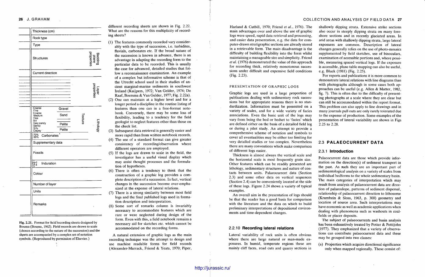
26 J .GRAHAM
Thickness (cm)
Rock type
Type
Structures O "O CD III CD (Q 0)
Current direction
"O
CD -< CD
Coarse Fine Coarse Medium Fine Silt Very sandy Sandy Silty Clayey
Gravel
Sand
Pelite
Pelite
c CD O O CO
Carbonates
Supplementary data
Fossils
Induration
Colour
Number of layer
Units
Remarks
Fig. 2.21. Format for fieldTecording sheets designed by Bouma (Bouma, 1962). Field records are drawn to scale (chosen according to the nature of the succession) and the sheets are accompanied by a complex set of notation symbols. (Reproduced by permission of Elsevier.)
different recording sheets are shown in Fig. 2.22. Wha t are the reasons for this multiplicity of recording sheets?
(1) The features commonly recorded vary considerably with the type of succession, i .e. turbidites, fluvials, carbonates etc. If the broad na ture of the succession is known in advance, there is an advantage in adapting the recording form to the particular da ta to be recorded. This is usually the case for advanced, detailed studies that follow a reconnaissance examinat ion. A n example of a complex but informative scheme is that of the Ut rech t school used in their studies of ancient marginal-marine sediments in southwest Ireland (Kuijpers, 1972; Van Gelder , 1974; D e Raaf, Boersma & Van Gelder , 1977; Fig. 2.22a).
(2) O n e can maintain at a higher level and for a longer period a discipline in the routine listing of features than one can in a free-format notebook. Conversely, there may be some loss of flexibility, leading to a tendency for the field geologist to neglect features o ther than those on the check list.
(3) Subsequent data retrieval is generally easier and more rapid than from written no tebook records.
(4) T h e use of a s tandard format can give greater consistency of recording/observation where different operators are employed.
(5) If the logs are drawn to scale in the field, the investigator has a useful visual display which may assist thought processes and the formulation of hypotheses.
(6) There is often a tendency to think that the construction of a graphic log provides a complete description of a succession. In fact, vertical changes in the succession become over-emphasized at the expense of lateral relations.
(7) There is a strong similarity between most field logs and the final published logs used in formation description and interpretat ion.
(8) Some sort of remarks column is invariably necessary to accommodate features which are rare or were neglected during design of the form. Even with this, a field notebook remains a necessary aid for sketches etc. which cannot be accommodated on the recording forms.
A natural extension of graphic logs as the main recording technique was the a t tempt to design and use machine readable forms for field records (Alexander-Marrack, Friend & Yeats , 1970; Piper,
COLLECTION AND ANALYSIS OF FIELD DATA 27
Harland & Cutbill, 1970; Friend et al., 1976). The main advantages over and above the use of graphic logs were speed, rapid data retrieval and processing, and easier data presentat ion, e.g. the data for computer-drawn stratigraphic sections are already stored in a retrievable form. The main disadvantage is the difficulty of building flexibility into the form whilst maintaining a manageable size and simplicity. Friend et al. (1976) demonstra ted the value of this approach for recording thick, relatively monotonous successions under difficult and expensive field conditions (Fig. 2.23).
P R E S E N T A T I O N O F G R A P H I C L O G S
Graphic logs are used in a large proport ion of publications dealing with sedimentary rock successions but for appropr ia te reasons there is no standardization. Information must be presented on a variety of scales, and for a wide variety of facies associations. Even the basic unit of the logs may vary from being the bed or bedset to 'facies' which are defined either on the basis of a detailed field log or during a pilot study. A n at tempt to provide a comprehensive scheme of notat ion and symbols to cover all eventualities may be either too limiting for very detailed studies or too complex. Nevertheless there are many conventions which make comparison of different logs easier.
Thickness is almost always the vertical scale and the horizontal scale is most frequently grain size. O the r features which can be readily presented are lithology, sedimentary structures and nature of contacts between units. Palaeocurrent data (Section 2.3) and some other data on vertical sequences (Section 2.4) can be conveniently located at the side of these logs. Figure 2.24 shows a variety of typical examples.
A n overall aim in the presentat ion of logs should be that the reader has a good basis for comparison with the l i terature and the data on which to build preliminary interpretat ions of depositional environments and t ime-dependent changes.
2.2.10 Recording lateral relations
Lateral variability of rock units is often obvious where there are large natural or man-made exposures . In humid, t empera te regions these are mainly cliff faces, road cuts and quarry sections in
shallowly dipping strata. Extensive strike sections also occur in steeply dipping strata on many foreshore sections and in recently glaciated areas. In arid areas with shallowly dipping strata, large lateral exposures are common. Description of lateral changes generally relies on the use of photo-mosaics supplemented by field sketches, use of binoculars, examination of accessible port ions and, where possible, measuring spaced vertical logs. If the exposure is accessible, plane table mapping can also be useful, e.g. Bluck (1981) (Fig. 2.25).
For reports and publications it is more common to demonst ra te lateral relations with line diagrams than with photographs although in some cases both approaches can b e useful (e .g. Allen & Mat ter , 1982, fig. 7) . This is often due to the difficulty of presenting photographs at a scale where they are clear but can still be accommodated within the report format. This problem can also apply to line drawings and in many journals pull outs are only rarely tolerated due to the expense of product ion. Some examples of the presentat ion of lateral variability are shown in Figs 2.25 to 2.28.
2.3 P A L A E O C U R R E N T D A T A
2.3.1 Introduction
Palaeocurrent data are those which provide informat ion on the direction(s) of sediment transport in the past. As such they are an important part of sedimentological analysis on a variety of scales from individual bedforms to the whole sedimentary basin. The main categories of interpretat ion which may result from analysis of palaeocurrent data are direction of palaeoslope, pat terns of sediment dispersal, relationship of palaeocurrent direction to l i thosome (Krumbein & Sloss, 1963, p . 300) geometry and location of source area. Such interpretat ions may have economic as well as academic applications when dealing with phenomena such as washouts in coalfields or placer deposits.
The subject of palaeocurrents and basin analysis has been exhaustively treated by Pot ter & Petti john (1977). They emphasized that a variety of observations can contr ibute palaeocurrent data and these may be grouped into two classes:
(a) Propert ies which acquire directional significance only when mapped regionally. These consist of:
http://jurassic.ru/
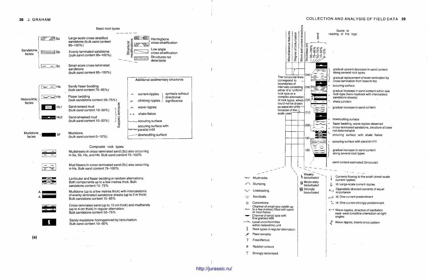
28 J .GRAHAM
Basic rock types
Sandstone facies
[ W Sa Large-scale cross-stratified sandstone (bulk sand content 95-100%)
Evenly laminated sandstone (bulk sand content 95-100%)
I\-"- \ Sc Small-scale cross-laminated sandstone (bulk sand content 95-100%)
Heterolithic facies
| Ha Sandy flaser bedding (bulk sand content 75-95%)
Flaser bedding (bulk sandstone content 50-75%) i
Hc1 Sand-lensed mud (bulk sand content 10-50%)
Hc2 Sand-streaked mud (bulk sand content 10-50%)
Mudstone _ ^ , Mudstone facies (bulk sand content 0-10%)
CO — c to o
« < «<ll Herringbone
Low angle cross-stratification Structures not detectable
Additional sedimentary structures
current-ripples "] symbols without > directional
climbing ripples J significance
wave-ripples
shale-flakes
-scouring surface scouring surface with
=-parallel infill - downcutting surface
Composite rock types Mudstreaks in cross-laminated sand (Sc) also occurring in Sa, Sb, Ha, and Hb. Bulk sand content 75-100%
Mud flasers in cross-laminated sand (Sc) also occurring in Ha. Bulk sand content 75-100%
Lenticular and flaser bedding in random alternations. Both components up to a few metres thick. Bulk sandstone content 10-75%
Mudstone (up to a few metres thick) with intercalations of evenly laminated sandstone sheets (up to 2 m thick) Bulk sandstone content 10-95%
Cross-laminated sand (up to 10 cm thick) and mudbands (up to 4 cm thick) in regular alternation. Bulk sandstone content 50-75%
Sandy mudstone homogenized by bioturbation. Bulk sand content 10-50%
(a)
COLLECTION AND ANALYSIS OF FIELD DATA
Guide to reading of the logs
iA J) i i T o en m i - o
The horizontal lines correspond to — boundaries of intervals consisting either of a 'uniform' rock type or a complex alternation of rock types, which could not be drawn as separate units — because of the 11 scale used
240 f 230
210
2001- 1 ^-"" 5
180
gradual upward decrease in sand content along several rock types gradual replacement of even lamination by cross-lamination from base to top scouring surface
gradual increase in sand content within one rock-type (here mudrock with intercalated sandstone sheets) sharp junction
gradual increase in sand content
downcutting surface flaser bedding, wave-ripples observed cross-laminated sandstone, structure at base not determinable
scouring surface with shale flakes
scouring surface with parallel infill
gradual increase in sand content along several rock types
sand content estimated (binocular)
Mudcracks
Slumping
Loadcasting
Sandballs
Concretions Channel of small size (width up to a few metres) filled with sand or mud-flakes Channel of small size with fine grained infill Local unconformities within heterolithic unit
Rock types in regular alternation Plant remains
Fossiliferous
Reddish colours
Strongly tectonized
. Weakly \ bioturbated U Moderately
bioturbated \\\ Strongly
bioturbated
| Currents flowing to the south (small-scale » current ripples) JJ, Id. Large-scale current ripples
, Oppositely directed currents of equal * importance
^ Id. One current predominant
\ Id. One current strongly predominant
*—> Wave-ripples, direction of oscillation east-west (crestline orientation at right angles
^ Wave ripples, interference pattern
http://jurassic.ru/
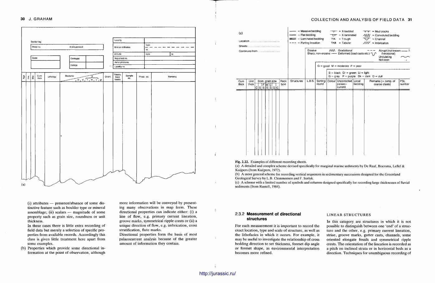
30 J . GRAHAM
Section log
Sheet no.
Geologist
Date(s)
Locality
Grid co-ordinates from
to
Altitude from | to
Map sheet no.
Aerial photo no.
Locality no.
Cum-thick
Lithology Fossils,
trace fossils
Sample
(b)
(i) at tr ibutes — presence/absence of some distinctive feature such as boulder type or mineral assemblage; (ii) scalars — magnitude of some proper ty such as grain size, roundness or unit thickness. In these cases there is little extra recording of field data but merely a selection of specific properties from available records. Accordingly this class is given little t rea tment here apart from some examples. Propert ies which provide some directional information at the point of observation, al though
more information will be conveyed by presenting many observations in map form. These directional propert ies can indicate ei ther: (i) a line of flow, e.g. pr imary current l ineation, groove marks , symmetrical ripple crests or (ii) a unique direction of flow, e.g. imbricat ion, cross stratification, flute marks . Directional propert ies form the basis of most palaeocurrent analysis because of the greater amount of information they contain.
COLLECTION AND ANALYSIS OF FIELD DATA 31
(0
Location
Sheets
Continues f rom.
• Massive bedding •• Flat bedding • Laminated bedding • Parting lineation
= X-bedded v v = Mud cracks = X-laminated JW\J = Convoluted bedding = Trough v_/ = Channel = Tabular / / / / = Imbrication
Erosive AA/\ Gradational Abrupt (not known -
Sharp, non-erosive Deformed (load casts etc.) "\J^ if erosional) Undulating -Not seen
G = good M = moderate P = poor
B = black Gr = green Lt = light G = grey P = purple Dk = dark D = dull
Cum thick
Unit thick
Pom, grain size F
clsls M C S S l G I C
Rock type
Structures L.B.S. Sorting/ round
Colour Uncorrected palaeo-
Local bedding
Remarks (+ comp. of coarse clasts)
PSL number
Fig. 2.22. Examples of different recording sheets. (a) A detailed and complex scheme devised specifically for marginal marine sediments by De Raaf, Boersma, Leflef & Kuijpers (from Kuijpers, 1972). (b) A more general scheme for recording vertical sequences in sedimentary successions designed for the Greenland Geological Survey by L.B. Clemmensen and F. Surlyk. (c) A scheme with a limited number of symbols and columns designed specifically for recording large thicknesses of fluvial sediments (from Russell, 1984).
2.3.2 Measurement of directional structures
For each measurement it is important to record the exact location, type and scale of s tructure, as well as the lithofacies in which it occurs. For example , it may be useful to investigate the relationship of cross bedding direction to set thickness, foreset dip angle or foreset shape, as environmental interpretat ion becomes more refined.
L I N E A R S T R U C T U R E S
In this category are structures in which it is not possible to distinguish between one ' end ' of a structure and the o ther , e.g. primary current l ineation, striae, groove marks , gutter casts, channels, some oriented elongate fossils and symmetrical ripple crests. T h e orientat ion of the lineation is recorded as a pitch on inclined strata or in horizontal beds as a direction. Techniques for unambiguous recording of
http://jurassic.ru/
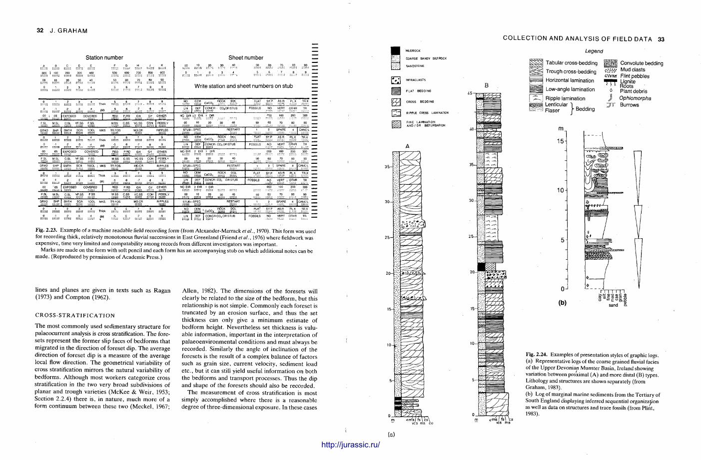
32 J.GRAHAM
Station number Sheet number A B C D E F G H J K 10 20 _ 30 _ 40 ^ 50 60 70 80 -.90
100 200 300 400 500 600 700 800 900 0 1 2 3 4 5 6 ' 7 8 _ - . 9 .
00
0 2 _
__30
3
40
4 5 6
70
7
SO
_ 8 _
90
9 Write station and sheet numbers on stub
0 =:!:=
2 4 Thick . . 6 . - 7 _ . A . NO CEM ROCK DOL
CaC0 3 : : : : r
FLAT SY.P AS.R PL.X TR.X
•0 •i .:?-. •4 (M) 7 •9 LIN DEF CONCR - C0 3 ORSTUB FOSSILS NO VERT OTHR TR
•00 | «_ EXPOSED COVERED I _RED F\RD _GY_ OTHER NO DIR | 2 DIR 1 DIR "00 100 200 300
F.SL M.SL C.SL VF.SS F.SS_ M_SS C.SS VC.SS ?. 0 N. PEBBLY 00 10 20 30 40 50 60 70 80 90
GRAD SHP SMTH SCR TOOL MKS TR.FOS MD ;CR RIPPLES STUB-—SPEC RESTART 2 SPARE 4 CANC'L
.9. 1 2 .A 4 Thick
5 _6_ 7 9 NO CEM ROCK DOL CaCO.1 : : : : :
FLAT SY.P AS.R PL.X TR.X
-0 •1 •2 •3 (M) •5 •6 •7 •9 LIN CONCR- COj OR STUB FOSSILS NO VERT OTHR TR
•00 EXPOSED COVERED | _RED P.RD ^GN_ -9.X. OTHER NO DIR 2 DIR 1 DIR 000 100 200 300
F.SL M.SL C.SL VF.SS F.SS M.SS C.SS VC.SS CON PEBBLY 00 10 20 30 40 50 60 70 80 90
GRAD SHP SMTH SCR TOOL | MKS TR.FOS. MD.CR RIPPLES STUB- -SPEC RESTART 1 SPARE =!,
CANC'L
—9.. :~=
2 3 ::::: Thick 5 6 7 8 9 NO CEM
c»co3 ?S5 :
K f ? i FLAT SY.P AS.R PL.X TR.X
•0 •2 -3 •4 (M) -5 •6 •7 •a 9 LIN CONCR- C 0 3 OR STUB FOSSILS NO VERT OTHR TR
•00 EXPOSED COVERED 1 RED P.RD GN GY OTHER NO DIR 2 DIR 1 DIR 000 100 200 300
F.SL M.SL C.SL VF.SS F.SS M.SS C.SS^ VC.SS CON PEBBLY 00 10 20 30 40 50 60 70 80 90
GRAD SHP SMTH SCR TOOL MKS. TR.FOS MD.CR RIPPLES STUB—SPEC RESTART 1 2 SPARE 4 CANC'L
0 __1. =
2 3 _ 4 Thick
5 6 7 B 9 NO CEM ROCK DOL CaC0 3 , -zzz:
FLAT SY.P AS.R PL.X TR.X
•0 ==-.:=
•2 -3 •4 (M) •5 -6 -7 •8 •9 LIN CONCR-C0 3 OR STUf3 FOSSILS NO VERT OTHR TR
Fig. 2.23. Example of a machine readable field recording form (from Alexander-Marrack etal., 1970). This form was used for recording thick, relatively monotonous fluvial successions in East Greenland (Friend et al., 1976) where fieldwork was expensive, time very limited and compatability among records from different investigators was important.
Marks are made on the form with soft pencil and each form has an accompanying stub on which additional notes can be made. (Reproduced by permission of Academic Press.)
lines and planes are given in texts such as Ragan (1973) and Compton (1962).
C R O S S - S T R A T I F I C A T I O N
T h e most commonly used sedimentary structure for palaeocurrent analysis is cross stratification. The fore-sets represent the former slip faces of bedforms that migrated in the direction of foreset dip. T h e average direction of foreset dip is a measure of the average local flow direction. T h e geometrical variability of cross stratification mirrors the natural variability of bedforms. Al though most workers categorize cross stratification in the two very broad subdivisions of planar and trough varieties (McKee & Weir , 1953; Section 2.2.4) there is, in na ture , much more of a form continuum between these two (Meckel , 1967;
Allen, 1982). The dimensions of the foresets will clearly be related to the size of the bedform, but this relationship is not simple. Commonly each foreset is t runcated by an erosion surface, and thus the set thickness can only give a minimum estimate of bedform height. Nevertheless set thickness is valuable information, important in the interpretat ion of palaeoenvironmental conditions and must always be recorded. Similarly the angle of inclination of the foresets is the result of a complex balance of factors such as grain size, current velocity, sediment load etc . , but it can still yield useful information on both the bedforms and transport processes. Thus the dip and shape of the foresets should also be recorded.
T h e measurement of cross stratification is most simply accomplished where there is a reasonable degree of three-dimensional exposure. In these cases
M i l l !
El
MUOROCK coarse SANDY siltrock sandstone
intraclasts
[ =| flat beoding
cross beoding
j2̂ | ripple cross lamination
fine lamination fc-r-Ij AND / OR BIOTURBATION
20-
COLLECTION AND ANALYSIS OF FIELD DATA 33
Legend
Convolute bedding
35-
2 5 -
20-
10-+
mm Tabular cross-bedding Trough cross-bedding Mud clasts
i'sms Flint pebbles Horizontal lamination ''
Low-angle lamination
1̂] Ripple lamination j s Lenticular "|
Flaser f Bedding
m.
15
k ' 9 n i t e
' * 1 Roots 6 Plant debris
J Ophiomorpha ~JT Burrows
10H
0 (b)
1 1 1 1 1 1 1 ffl ' in c n) at to ~
sand
Fig. 2.24. Examples of presentation styles of graphic logs. (a) Representative logs of the coarse grained fluvial facies of the Upper Devonian Munster Basin, Ireland showing variation between proximal (A) and more distal (B) types. Lithology and structures are shown separately (from Graham, 1983). (b) Log of marginal marine sediments from the Tertiary of South England displaying inferred sequential organization as well as data on structures and trace fossils (from Plint, 1983).
(a)
http://jurassic.ru/
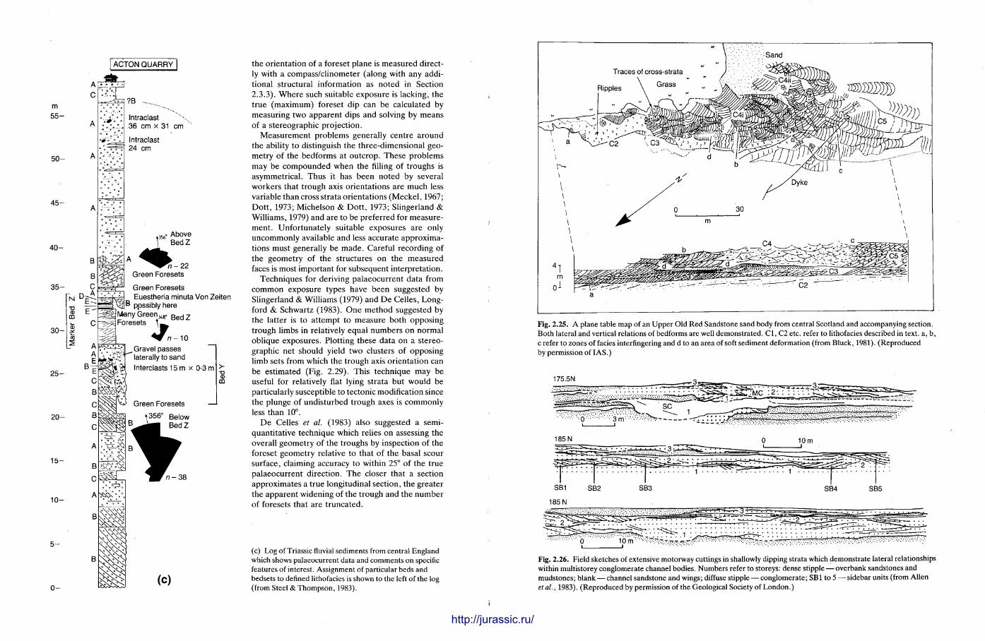
m 55-
50-
45-
40-
3 5 -
30-
2 5 -
20-
15-
10-
Intraclast 36 cm x 31 cm
Intraclast 24 cm
. Above » S 6 '
\ BedZ
"77-22 Green Foresets
Green Foresets ^ Euestheria minuta Von Zeiten Vj|B ppssiblyhere Many Green,,,,. B e d z
Foresets \ fc
n-10 Gravel passes laterally to sand fiSi* ?H Interclasts 15 m x 0-3 m I >"
. 0> m
Green Foresets
\356° Below BedZ
(c)
the orientation of a foreset plane is measured directly with a compass/clinometer (along with any additional structural information as noted in Section 2.3.3). Where such suitable exposure is lacking, the t rue (maximum) foreset dip can be calculated by measuring two apparent dips and solving by means of a stereographic projection.
Measurement problems generally centre around the ability to distinguish the three-dimensional geometry of the bedforms at outcrop. These problems may be compounded when the filling of t roughs is asymmetrical . Thus it has been noted by several workers that trough axis orientat ions are much less variable than cross strata orientat ions (Meckel , 1967; Dot t , 1973; Michelson & Dot t , 1973; Slingerland & Williams, 1979) and are to be preferred for measurement . Unfortunately suitable exposures are only uncommonly available and less accurate approximations must generally be made . Careful recording of the geometry of the structures on the measured faces is most important for subsequent interpretation.
Techniques for deriving palaeocurrent data from common exposure types have been suggested by Slingerland & Williams (1979) and De Celles, Longford & Schwartz (1983). O n e method suggested by the latter is to a t tempt to measure both opposing trough limbs in relatively equal numbers on normal oblique exposures. Plotting these data on a stereo-graphic net should yield two clusters of opposing limb sets from which the trough axis orientat ion can be estimated (Fig. 2.29). This technique may be useful for relatively flat lying strata but would be particularly susceptible to tectonic modification since the plunge of undisturbed trough axes is commonly less than 10°.
D e Celles et al. (1983) also suggested a semiquanti tat ive technique which relies on assessing the overall geometry of the troughs by inspection of the foreset geometry relative to that of the basal scour surface, claiming accuracy to within 25° of the t rue palaeocurrent direction. The closer that a section approximates a t rue longitudinal section, the greater the apparent widening of the trough and the number of foresets that are t runcated.
(c) Log of Triassic fluvial sediments from central England which shows palaeocurrent data and comments on specific features of interest. Assignment of particular beds and bedsets to defined lithofacies is shown to the left of the log (from Steel & Thompson, 1983).
HIIHIIHIimiHimiHIIHIHIIWfflllHIll
Fig. 2.25. A plane table map of an Upper Old Red Sandstone sand body from central Scotland and accompanying section. Both lateral and vertical relations of bedforms are well demonstrated. CI, C2 etc. refer to lithofacies described in text, a, b, c refer to zones of facies interfingering and d to an area of soft sediment deformation (from Bluck, 1981). (Reproduced by permission of IAS.)
Fig. 2.26. Field sketches of extensive motorway cuttings in shallowly dipping strata which demonstrate lateral relationships within multistorey conglomerate channel bodies. Numbers refer to storeys: dense stipple -— overbank sandstones and mudstones; blank — channel sandstone and wings; diffuse stipple — conglomerate; SB 1 to 5 — sidebar units (from Allen et al., 1983). (Reproduced by permission of the Geological Society of London.)
http://jurassic.ru/
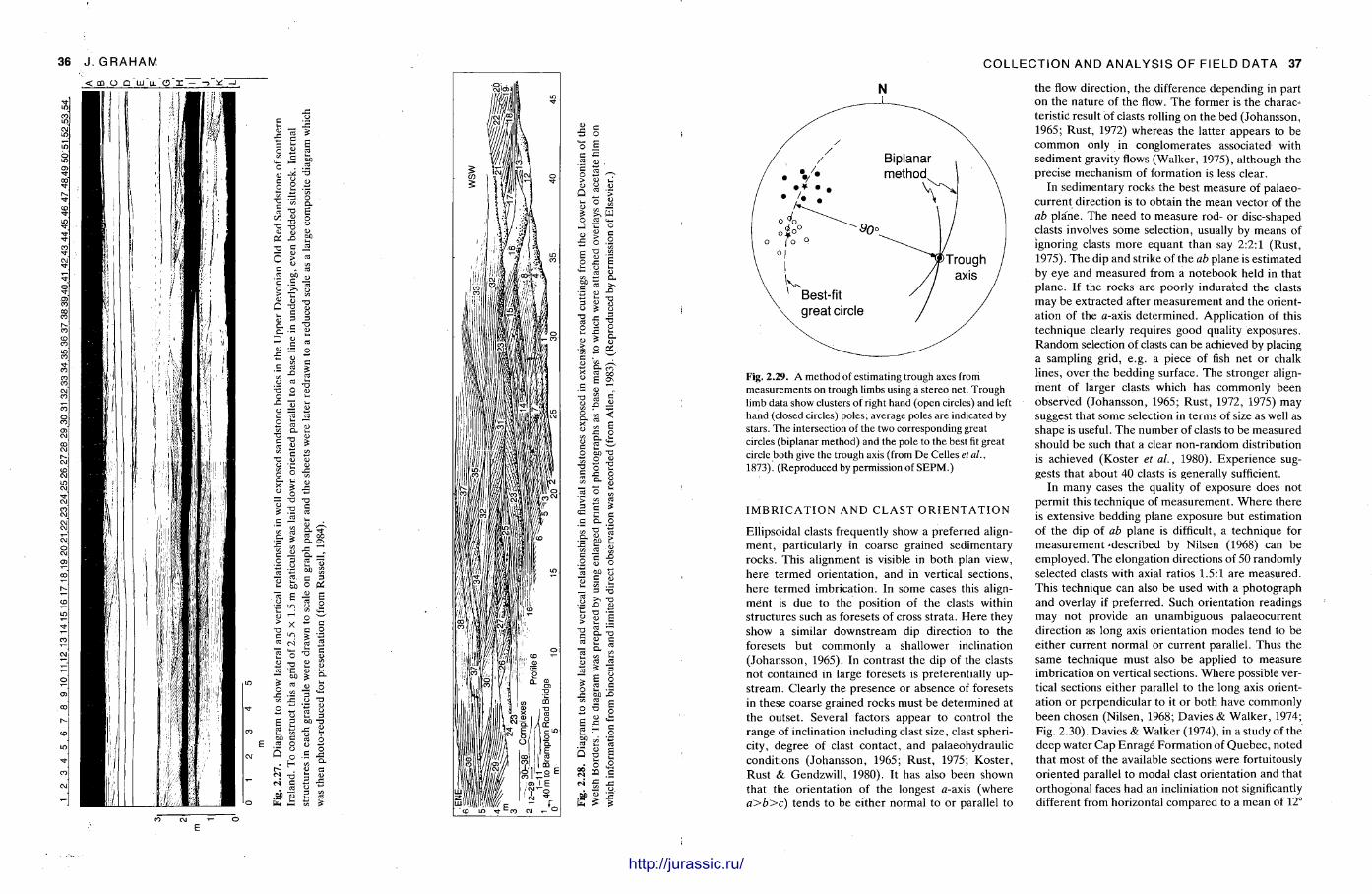
COLLECTION AND ANALYSIS OF FIELD DATA 37
£ 00
o a o
« D. •a E •8 °
Q "a 3 •- 3 3 U 3 3 a c " a - S 3 £ a S = 2
« c E a s
O ° -5
^ 2 "S
9-cd oo CL Ov D. _T 2 U M 2
00 ° s -3
o •a - _ <u - oo ^
o a £ a
a> o
~ O ^ „. e 3 oo -o 5 h _ o
^ -a 3 2 « . S | « b i S S
o E
o
•s u 3 13 O
T3 O O S g-
O £< c -s S- <̂> u E " •E o 1
•s 1 I S •» E
•a o a 5 -c o 5 a ° — .2 ° M > j2 5
•o oo
en , J2
Fig. 2.29. A method of estimating trough axes from measurements on trough limbs using a stereo net. Trough limb data show clusters of right hand (open circles) and left hand (closed circles) poles; average poles are indicated by stars. The intersection of the two corresponding great circles (biplanar method) and the pole to the best fit great circle both give the trough axis (from De Celles etal., 1873). (Reproduced by permission of SEPM.)
I M B R I C A T I O N A N D C L A S T O R I E N T A T I O N
Ellipsoidal clasts frequently show a preferred alignment , particularly in coarse grained sedimentary rocks. This alignment is visible in both plan view, here te rmed orientat ion, and in vertical sections, here te rmed imbrication. In some cases this alignment is due to the position of the clasts within structures such as foresets of cross strata. He re they show a similar downstream dip direction to the foresets but commonly a shallower inclination (Johansson, 1965). In contrast the dip of the clasts not contained in large foresets is preferentially upstream . Clearly the presence or absence of foresets in these coarse grained rocks must be determined at the outset . Several factors appear to control the range of inclination including clast size, clast sphericity, degree of clast contact , and palaeohydraulic conditions (Johansson, 1965; Rust , 1975; Koster , Rust & Gendzwill , 1980). It has also been shown that the orientation of the longest a-axis (where a>b>c) tends to be either normal to or parallel to
the flow direction, the difference depending in part on the nature of the flow. The former is the characteristic result of clasts rolling on the bed (Johansson, 1965; Rust , 1972) whereas the latter appears to be common only in conglomerates associated with sediment gravity flows (Walker , 1975), although the precise mechanism of formation is less clear.
In sedimentary rocks the best measure of palaeocurrent direction is to obtain the mean vector of the ab pla'ne. The need to measure rod- or disc-shaped clasts involves some selection, usually by means of ignoring clasts more equant than say 2:2:1 (Rust , 1975). T h e dip and strike of the ab plane is estimated by eye and measured from a notebook held in that plane. If the rocks are poorly indurated the clasts may be extracted after measurement and the orientation of the a-axis de termined. Application of this technique clearly requires good quality exposures. Random selection of clasts can be achieved by placing a sampling grid, e.g. a piece of fish net or chalk lines, over the bedding surface. The stronger alignment of larger clasts which has commonly been observed (Johansson, 1965; Rust , 1972, 1975) may suggest that some selection in terms of size as well as shape is useful. The number of clasts to be measured should be such that a clear non-random distribution is achieved (Koster et al., 1980). Experience suggests that about 40 clasts is generally sufficient.
In many cases the quality of exposure does not permit this technique of measurement . Where there is extensive bedding plane exposure but estimation of the dip of ab p lane is difficult, a technique for measurement 'described by Nilsen (1968) can be employed. The elongation directions of 50 randomly selected clasts with axial ratios 1.5:1 are measured. This technique can also be used with a photograph and overlay if preferred. Such orientation readings may not provide an unambiguous palaeocurrent direction as long axis orientat ion modes tend to be either current normal or current parallel. Thus the same technique must also be applied to measure imbrication on vertical sections. Where possible vertical sections either parallel to the long axis orientation or perpendicular to it or both have commonly been chosen (Nilsen, 1968; Davies & Walker , 1974; Fig. 2.30). Davies & Walker (1974), in a study of the deep water Cap Enrage Format ion of Quebec , noted that most of the available sections were fortuitously oriented parallel to modal clast orientation and that or thogonal faces had an incliniation not significantly different from horizontal compared to a mean of 12°
http://jurassic.ru/
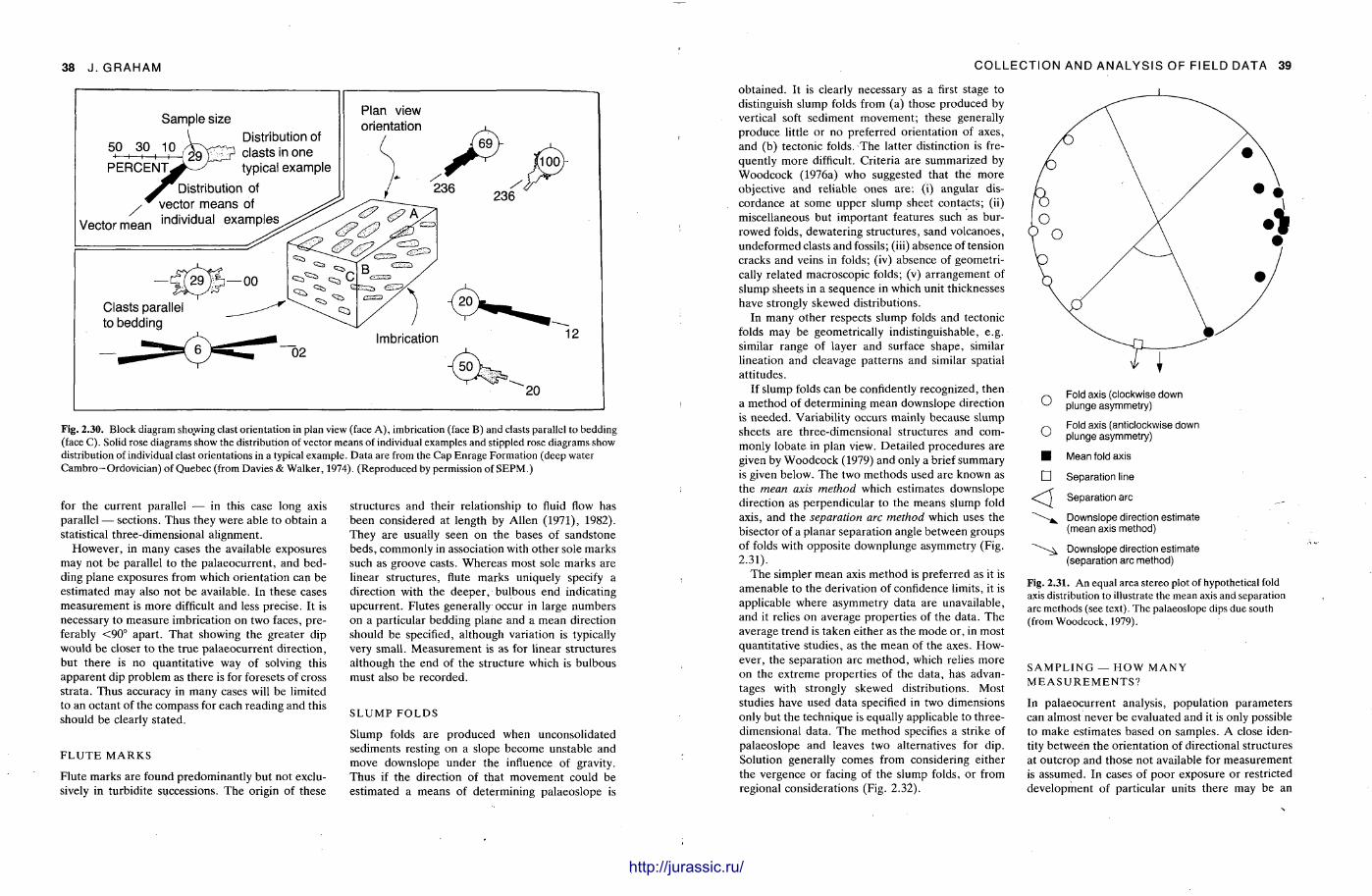
38 J . GRAHAM
Sample size
50 30 10 -i—i—i—^
PERCENT W
Distribution of vector means of
Vector mean individual examples
Distribution of clasts in one typical example
Plan view orientation
Clasts parallel to bedding
Fig. 2.30. Block diagram showing clast orientation in plan view (face A), imbrication (face B) and clasts parallel to bedding (face C). Solid rose diagrams show the distribution of vector means of individual examples and stippled rose diagrams show distribution of individual clast orientations in a typical example. Data are from the Cap Enrage Formation (deep water Cambro-Ordovician) of Quebec (from Davies & Walker, 1974). (Reproduced by permission of SEPM.)
for the current parallel — in this case long axis parallel — sections. Thus they were able to obtain a statistical three-dimensional alignment.
However , in many cases the available exposures may not be parallel to the palaeocurrent , and bedding plane exposures from which orientat ion can be est imated may also not be available. In these cases measurement is more difficult and less precise. It is necessary to measure imbrication on two faces, preferably <90° apart . Tha t showing the greater dip would be closer to the t rue palaeocurrent direction, but there is no quanti tat ive way of solving this apparent dip problem as there is for foresets of cross strata. Thus accuracy in many cases will be limited to an octant of the compass for each reading and this should be clearly stated.
F L U T E M A R K S
Flute marks are found predominantly but not exclusively in turbidite successions. The origin of these
structures and their relationship to fluid flow has been considered at length by Allen (1971), 1982). They are usually seen on the bases of sandstone beds, commonly in association with other sole marks such as groove casts. Whereas most sole marks are linear structures, flute marks uniquely specify a direction with the deeper , bulbous end indicating upcurrent . Flutes generally occur in large numbers on a particular bedding plane and a mean direction should be specified, al though variation is typically very small. Measurement is as f oT linear structures al though the end of the structure which is bulbous must also be recorded.
S L U M P F O L D S
Slump folds are produced when unconsolidated sediments resting on a slope become unstable and move downslope under the influence of gravity. Thus if the direction of that movement could be est imated a means of determining palaeoslope is
iHimimiHiiHummiinHiif im
COLLECTION AND ANALYSIS OF FIELD DATA 39
obtained. It is clearly necessary as a first stage to distinguish slump folds from (a) those produced by vertical soft sediment movement ; these generally produce little or no preferred orientation of axes, and (b) tectonic folds. The latter distinction is frequently more difficult. Criteria are summarized by Woodcock (1976a) who suggested that the more objective and reliable ones are: (i) angular discordance at some upper slump sheet contacts; (ii) miscellaneous but important features such as burrowed folds, dewatering structures, sand volcanoes, undeformed clasts and fossils; (iii) absence of tension cracks and veins in folds; (iv) absence of geometrically related macroscopic folds; (v) ar rangement of slump sheets in a sequence in which unit thicknesses have strongly skewed distributions.
In many other respects slump folds and tectonic folds may be geometrically indistinguishable, e.g. similar range of layer and surface shape, similar lineation and cleavage pat terns and similar spatial at t i tudes.
If slump folds can be confidently recognized, then a method of determining mean downslope direction is needed . Variability occurs mainly because slump sheets are three-dimensional structures and commonly lobate in plan view. Detai led procedures are given by Woodcock (1979) and only a brief summary is given below. The two methods used are known as the mean axis method which estimates downslope direction as perpendicular to the means slump fold axis, and the separation arc method which uses the bisector of a planar separation angle between groups of folds with opposite downplunge asymmetry (Fig. 2.31).
T h e simpler mean axis method is preferred as it is amenable to the derivation of confidence limits, it is applicable where asymmetry data are unavailable, and it relies on average propert ies of the data. The average t rend is taken either as the mode or, in most quanti tat ive studies, as the mean of the axes. However, the separation arc method , which relies more on the ext reme propert ies of the data , has advantages with strongly skewed distributions. Most studies have used data specified in two dimensions only but the technique is equally applicable to three-dimensional data. The method specifies a strike of palaeoslope and leaves two alternatives for dip. Solution generally comes from considering either the vergence or facing of the slump folds, or from regional considerations (Fig. 2.32).
o o • •
Fold axis (clockwise down plunge asymmetry)
Fold axis (anticlockwise down plunge asymmetry)
Mean fold axis
Separation line
Separation arc
Downslope direction estimate (mean axis method)
Downslope direction estimate (separation arc method)
Fig. 2.31. An equal area stereo plot of hypothetical fold axis distribution to illustrate the mean axis and separation arc methods (see text). The palaeoslope dips due south (from Woodcock, 1979).
S A M P L I N G — H O W M A N Y M E A S U R E M E N T S ?
In palaeocurrent analysis, population parameters can almost never be evaluated and it is only possible to make estimates based on samples. A close identity between the orientation of directional structures at outcrop and those not available for measurement is assumed. In cases of poor exposure or restricted development of particular units there may be an
http://jurassic.ru/
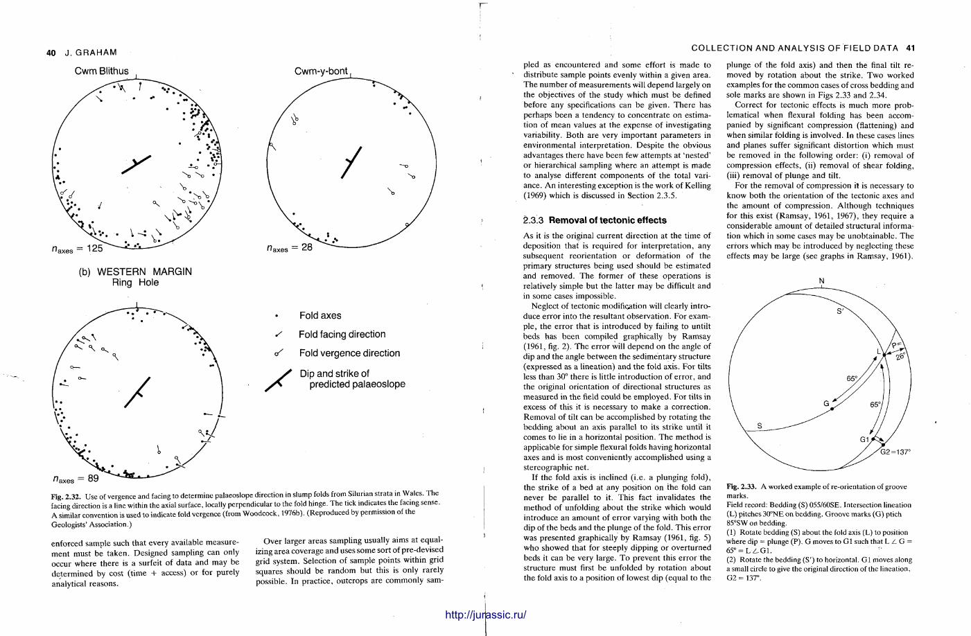
40 J .GRAHAM
Cwm Blithus Cwm-y-bont
(b) WESTERN MARGIN Ring Hole
n — RQ ""*"--*-AaL»—»-" a x e s
Fold axes
s Fold facing direction
</ Fold vergence direction
X Dip and strike of predicted palaeoslope
Fig. 2.32. Use of vergence and facing to determine palaeoslope direction in slump folds from Silurian strata in Wales. The facing direction is a line within the axial surface, locally perpendicular to the fold hinge. The tick indicates the facing sense. A similar convention is used to indicate fold vergence (from Woodcock, 1976b). (Reproduced by permission of the Geologists' Association.)
enforced sample such that every available measurement must be taken. Designed sampling can only occur where there is a surfeit of data and may be determined by cost (t ime + access) or for purely analytical reasons.
Over larger areas sampling usually aims at equalizing area coverage and uses some sort of pre-devised grid system. Selection of sample points within grid squares should be random but this is only rarely possible. In practice, outcrops are commonly sam-
COLLECTION AND ANALYSIS OF FIELD DATA 41
pled as encountered and some effort is made to distribute sample points evenly within a given area. The number of measurements will depend largely on the objectives of the study which must be defined before any specifications can be given. There has perhaps been a tendency to concentrate on estimation of mean values at the expense of investigating variability. Both are very important parameters in environmental interpretat ion. Despite the obvious advantages there have been few at tempts at 'nested ' or hierarchical sampling where an a t tempt is made to analyse different components of the total variance. A n interesting exception is the work of Kelling (1969) which is discussed in Section 2.3.5.
2.3.3 Removal of tectonic effects
As it is the original current direction at the time of deposition that is required for interpretat ion, any subsequent reorientat ion or deformation of the primary structures being used should be estimated and removed. The former of these operat ions is relatively simple but the latter may be difficult and in some cases impossible.
Neglect of tectonic modification will clearly introduce error into the resultant observation. For example, the error that is introduced by failing to untilt beds has been compiled graphically by Ramsay (1961, fig. 2). The error will depend on the angle of dip and the angle between the sedimentary structure (expressed as a lineation) and the fold axis. For tilts less than 30° there is little introduction of error , and the original orientat ion of directional structures as measured in the field could be employed. For tilts in excess of this it is necessary to make a correction. Removal of tilt can be accomplished by rotating the bedding about an axis parallel to its strike until it comes to lie in a horizontal position. The method is applicable for simple flexural folds having horizontal axes and is most conveniently accomplished using a stereographic net .
If the fold axis is inclined (i .e. a plunging fold), the strike of a bed at any position on the fold can never be parallel to it. This fact invalidates the method of unfolding about the strike which would introduce an amount of error varying with both the dip of the beds and the plunge of the fold. This error was presented graphically by Ramsay (1961, fig. 5) who showed that for steeply dipping or overturned beds it can be very large. To prevent this error the structure must first be unfolded by rotation about the fold axis to a position of lowest dip (equal to the
plunge of the fold axis) and then the final tilt removed by rotation about the strike. Two worked examples for the common cases of cross bedding and sole marks are shown in Figs 2.33 and 2.34.
Correct for tectonic effects is much more problematical when flexural folding has been accompanied by significant compression (flattening) and when similar folding is involved. In these cases lines and planes suffer significant distortion which must be removed in the following order: (i) removal of compression effects, (ii) removal of shear folding, (iii) removal of plunge and tilt.
For the removal of compression it is necessary to know both the orientation of the tectonic axes and the amount of compression. Al though techniques for this exist (Ramsay, 1961, 1967), they require a considerable amount of detailed structural information which in some cases may be unobtainable . The errors which may be introduced by neglecting these effects may be large (see graphs in Ramsay, 1961).
G2=137°
Fig. 2.33. A worked example of re-orientation of groove marks. Field record: Bedding (S) 055/60SE. Intersection lineation (L) pitches 30°NE on bedding. Groove marks (G) ptich 85°SW on bedding. (1) Rotate bedding (S) about the fold axis (L) to position where dip = plunge (P). G moves to Gl such that L Z. G = 65° I . / . G 1 . (2) Rotate the bedding (S') to horizontal. Gl moves along a small circle to give the original direction of the lineation, G2 = 137°.
http://jurassic.ru/
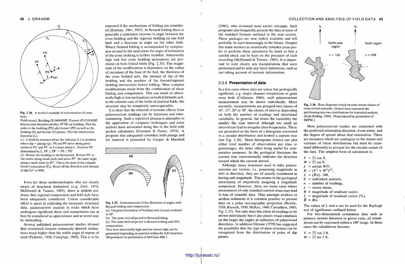
42 J .GRAHAM
N
Fig. 2.34. A worked example of reorientation of cross beds. Field record: Bedding (S) 040/40SE. Foreset (F) 010/48SE. Intersection lineation pitches 30°NE on bedding. Plot the poles to the bedding (PS) and foreset (PF) as well as the bedding (S) and foreset (F) planes. Plot the intersection lineation (L). (1) Unfold by rotation about the fold axis (L) to position where dip = plunge (p). PS and PF move along great circles to PS' and PF' as S rotates about L. Position PS' determined by L. PF Z. PF' = PS L PS'. (2) Rotate the bedding to the horizontal. Return PS' to the centre along small circle and move PF' the same angle along a small circle to PF". This is the pole of the original foreset orientation (F 0). Read off the direction and amount of dip (25° to 040).
Even for those sedimentologists who are clearly aware of structural limitations (e.g. Dot t , 1974; McDonald & Tanner , 1983), there is seldom evidence that regional compression and fold style have been adequately considered. Unless considerable effort is spent in collecting the necessary structural data , palaeocurrent analysis in rocks which have undergone significant shear and compression can at best be considered as approximate and at worst may be misleading.
Several published palaeocurrent studies showed that reoriented foresets commonly showed inclinations much higher than the stable angle of repose of sand (Pelletier, 1958; Cassyhap, 1968). This is to be
expected if the mechanisms of folding are considered (Ramsay, 1961, 1967). In flexural folding there is generally a systematic increase in angle between the cross bedding and the regional bedding on one fold limb and a decrease in angle on the other l imb. Where flexural folding is accompanied by compression normal to the axial plane the angle of inclination of the cross bedding is further modifed. Abnormal ly high and low cross bedding inclinations are produced on both folded limbs (Fig. 2.35). The magnitude of the modifications is dependent on the radius of curvature of the base of the bed, the thickness of the cross bedded unit, the amount of dip of the bedding and the position of the foreset/regional bedding intersection before folding. Most complex modifications result from the combination of shear folding and compression. This can result in abnormally high or low inclinations on both fold limbs and, in the extreme case of the limbs of isoclinal folds, the structure may be completely unrecognizable.
It is clear that the removal of tectonic effects from palaeocurrent readings can be laborious and t ime-consuming. Such a repetitive process is amenable to the application of computer techniques and some authors have advocated doing this in the field with pocket calculators (Freeman & Pierce, 1979). A program that adequately considers both plunge and tilt removal is presented by Cooper & Marshall
Fig. 2.35. Demonstration of the distortion of angles with flexural folding and compression. (a) Original orientation of bedding with foresets inclined at 30°. (b) The same bed subjected to flexural folding. (c) The same bed subjected to flexural folding and 50% compression. Note how abnormally high and low foreset dips can be generated depending on position within the fold structure. (Reproduced by permission of McGraw-Hill.)
COLLECTION AND ANALYSIS OF FIELD DATA 4 3
(1981), who reviewed most earlier a t tempts . Such programs also frequently present the data in some of the s tandard formats outlined in the next section. These packages are now widely available and will probably be used increasingly in the future. Despite this some workers in structurally complex areas prefer to perform these operat ions by hand so that a careful check can be kept on the precision of each recording (McDonald & Tanner , 1983). It is important to state clearly any manipulations that were performed and to note any likely limitations, such as not taking account of tectonic deformation.
2.3.4 Presentation of data
In a few cases where data are scarce but geologically significant, e.g. major channel orientat ions or giant cross beds (Collinson, 1968), each palaeocurrent measurement may be shown individually. More normally, measurements are grouped into classes of 10°, 15°, 20° or 30°, the choice of interval depending on both the number of readings and directional variability. In general , the lower the variability the smaller the class interval although too small an interval can lead to irregular class frequencies. These are presented in the form of a histogram converted to a circular distribution and termed a current rose (see Fig. 2.36). These histograms (roses) can plot either total number of observations per class or percentages , the latter often being useful for comparative purposes. In the geological l i terature the current rose conventionally indicates the direction toward which the current moved.
Although many structures used to infer palaeo-currents are vectors, i.e. possessing magnitude as well as direction, they are all usually considered as having unit magni tude. This relates to the geological uncertainty of objectively assigning a magni tude component . However , there are many cases where presentat ion of only s tandard current roses may lead to loss of valuable data . Thus amongst workers in aeolian sediments it is common practice to present data on a polar stereographic projection (Reiche, 1938; Kiersch, 1950; McKee , 1966; Carruthers , 1985; Fig. 2.37). Not only does this allow all readings to be shown individually but it also places visual emphasis on the larger dip angles as indicators of palaeowind directions. In addition Glennie (1970) has suggested the possibility that the type of dune structure can be recognized from the distribution of poles of dip planes.
N 4 North-east
region
n = 120
North region
n = 258
Fig. 2.36. Rose diagrams based on semi-octant classes of cross-stratal azimuths. Dotted lines represent the partitioning into two distributions for statistical analysis , (from Kelling, 1969). (Reproduced by permission of SEPM.)
Most palaeocurrent studies are concerned with the preferred orientation direction, if one exists, and the degree of spread about that orientat ion. These are measures which are analogous to the means and variance of linear distributions but must be calculated differently to account for the circular nature of the data . The simplest form of calculation is:
V = £" cos 6, W = E',' sin 9, x = arctan WIV, R = (v2 + w2y/2, L = (R/n). 100, 0 = individual azimuth, n = number of readings, x = vector mean , R = magni tude of resultant vector, L = magni tude of resultant vector ( % ) . R = R/n
The values of L and n can be used for the Rayleigh test of significance outlined below.
For two-dimensional orientat ion data such as primary current lineation or goove casts, all orientations can be expressed within a 180° range. In these cases the calculations become:
V = Li cos 2 0, W = £" sin 2 9,
http://jurassic.ru/
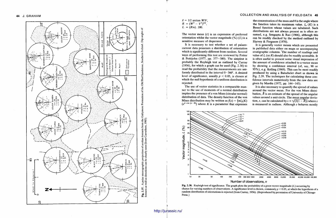
44 J . GRAHAM COLLECTION AND ANALYSIS OF FIELD DATA 45
x = 1/2 arctan WIV, R = (w2 - V2)1'2, L = (Rlri). 100.
The vector mean (x) is an expression of preferred orientat ion whilst the vector magni tude (%) (L) is a sensitive measure of dispersion.
It is necessary to test whether a set of palaeocurrent data possesses a distribution of orientation which is significantly different from random. Several ways of performing this test are reviewed by Pot ter & Petti john (1977, pp . 3 7 7 - 3 8 0 ) . The simplest is probably the Rayleigh test as outlined by Curray (1956), for which a graph can be used (Fig. 2.38) to read the probability that t he measurements a re uniformly distributed in the interval 0—360°. A desired level of significance, usually p < 0.05, is chosen at which the null hypothesis of a uniform distribution is rejected.
T h e use of vector statistics in a comparable manner to the use of moments of a normal distribution implies the presence of a von Mises (circular normal) distribution of da ta . T h e density function of the von Mises distribution may be written as f(x) = jnI0(K) (ek c o s ( x _ e ) ) where K is a pa ramete r that expresses
the concentrat ion of the mass and 8 is the angle where the function takes its maximum value. I0 (K) is a Bessel function whose values are tabulated. Such distributions are not always present as is often assumed, e.g. Sengupta & R a o (1966), al though this can be readily checked by the method outlined by Harvey & Ferguson (1976).
It is generally vector means which are presented in published data ei ther on maps or accompanying stratigraphic columns. "The number of readings and value of L (or R) should also be readily accessible. It is often useful to present some visual impression of t he amoun t of confidence at tached to a vector mean by showing a confidence interval (of, say, 90 or 9 5 % ) , e.g. Kelling (1969). This can be most readily p roduced by using a Batschelet chart as shown in Fig. 2.39. The techniques for calculating these confidence intervals numerically from the raw data are given by Mardia (1972, pp . 144—145).
It is also necessary to quantify the spread of values around the vector mean. For the von Mises distribution, R is an est imate of the spread of the angular values a round a unit circle. The mean angular deviation, s, can be calculated by s = V(2(l — R)) where s is measured in radians. Al though s behaves mostly
1 0 20 50 100 200 400 600 800 1000 2000 4000 6000 10,000 20,000 40,000 60,000 100,000
Number of observations, n Fig. 2.38. Rayleigh test of significance. The graph plots the probability of a given vector magnitude (L) occurring by chance for varying numbers of observations. A significance level is chosen, commonly p < 0.05, at which the hypothesis of a random distribution of orientations is rejected (from Curray, 1956). (Reproduced by permission of University of Chicago Press.)
http://jurassic.ru/
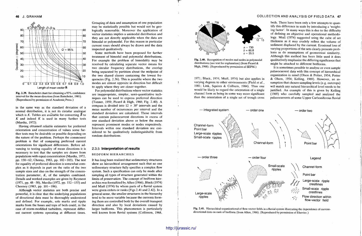
46 J . GRAHAM
0 0.1 0.2 0.3 0.4 6.5 0.6 0.7 0.8 0.9 1.0 Length of mean vector R
Fig. 2.39. Batschelet chart for obtaining a 95% confidence ipterval for the mean direction (from Batschelet, 1981). (Reproduced by permission of Academic Press.)
in the same way as the s tandard deviation of a normal distribution, it is not its circular analogue which is K. Tables are available for converting R to K and indeed K is used in many further tests (Mardia , 1972).
Having obtained reliable estimates for preferred orientation and concentrat ion of values some further tests may be desirable or possible depending on the na ture of the problem. Perhaps the commonest problem is that of comparing preferred current orientat ions for significant differences. Before advancing to testing equality of mean directions it is necessary to test that the samples are drawn from populat ions with equal concentrat ion (Mardia , 1972, pp . 1 5 8 - 6 2 ; Cheeny, 1983, pp . 102 -103) . T h e test for equality of preferred direction is somewhat complex as it depends in part on the ratio of the two sample sizes and also on the strength of the concentration parameter , K, of the samples combined. Details and worked examples are given by Reyment (1971, pp . 4 8 - 5 0 ) , Mardia (1972, pp . 152 -155 ) and Cheeney (1983, pp . 1 0 1 - 1 0 6 ) .
Al though vector statistics are both precise and powerful, it is clear that the underlying populat ions of directional data must be thoroughly unders tood and defined. For example , sole marks and ripple marks from the bases and tops of beds could, in the case of storm-modified turbidites, represent different current systems operat ing at different t imes.
Grouping of data and assumption of one populat ion may be statistically possible but would not be geologically reasonable . Moreover the application of vector statistics implies a unimodal distribution and they are not directly applicable when the data are bimodal or polymodal . For this reason in particular current roses should always be drawn and the data inspected qualitatively.
Some methods have been proposed for further t rea tment of bimodal and polymodal distributions. For example the problem of bimodality may be resolved by calculating separate vector means for two circular frequency distributions, the overlap being separated by partit ion about the midpoint of the two shared classes containing the lowest frequencies (Fig. 2.36). This is possible where the two modes are almost opposite in direction but difficult to apply where they are closer together .
For polymodal distributions where vector statistics are inappropr ia te , simpler, semi-quantitative techniques can be used to express preferred direction (Tanner , 1959; Picard & High, 1968; Fig. 2.40). A compass is divided into 12 x 30° intervals and the mean number of occurrences per interval and the s tandard deviation are calculated. Those intervals that contain palaeocurrent directions in excess of one s tandard deviation above or below the mean represent prominent modes or nodes respectively. Intervals within one s tandard deviation are considered to be qualitatively indistinguishable from random distributions.
2.3.5 Interpretation of results
B E D F O R M H I E R A R C H I E S
It has long been realized that sedimentary structures show an hierarchical ar rangement such that no one sedimentary structure fully specifies a complex flow system. Such a specification can only be made after sampling all types of structure generated within the limits of preservation. The concept of bedform hierarchies was formalized by Allen (1966), Bluck (1974) and Miall (1974) by whom parts of a fluvial system were given orders or ranks (Figs 2.41 and 2.42). In a general sense, the smaller structures in the hierarchy tend to be more variable because the currents forming them are controlled both by the overall t ransport direction and also by local deviations caused by larger bedforms. This phenomenon is particularly well known from fluvial systems (Collinson, 1968,
1UJIM1
COLLECTION AND ANALYSIS OF FIELD DATA 47
10 15
Fig. 2.40. Recognition of modes and nodes in polymodal distributions (see text for explanation) (from Picard & High, 1968). (Reproduced by permission of SEPM.)
1971; Bluck, 1974; Miall, 1974) but also applies in varying degrees to o ther environments (Field et al., 1981; Link, Squires & Colburn , 1984). Thus one would be likely to regard the orientation of a single channel form as being in some way more significant than the orientation of a single set of trough cross
beds. There have been only a few at tempts to quantify this difference in scale by introducing a 'weighting factor' . In many ways this is due to the difficulty of defining an objective and operat ional methodology. Miall (1974) suggested using the cube of set thickness as it may crudely reflect the volume of sediment displaced by the current . Erosional loss of varying proport ions of the sets clearly presents problems as do assumptions of geometrical similarity. Al though this method has been little used it does qualitatively emphasize the differing significance that might be attached to different bedforms.
It is sometimes possible to analyse or even sample palaeocurrent data with this concept of hierarchical organization in mind (Olson & Pot ter , 1954; Potter & Olson, 1954; Kelling, 1969). However , an assumption that chosen sampling levels (e.g. outcrops) will match any natural hierarchical level needs to b e justified. A n example of this is given by Kelling (1969) who carefully sampled and analysed the palaeocurrents of some Uppe r Carboniferous fluvial
integrated system
Channel-form Point bar Large-scale ripples Small-scale ripples
• order one — order two
Channel-form
• order three — order four
Large-scale ripples
Small-scale ripples
„rrfc 1 r r r
Legend
Channel-form
Point bar
Large-scale ripple crestlines
Small-scale ripple crestlines
Flow direction within flow-vector field
Fig. 2.41. Hierarchical organizational of flow-vector fields in a fluvial system illustrating the dependence of current-directional data on rank of bedform (from Allen, 1966). (Reproduced by permission of Elsevier.)
lit http://jurassic.ru/
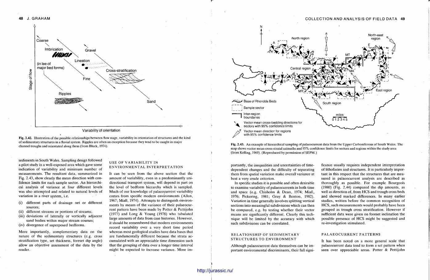
48 J . GRAHAM
Variability of orientation
Fig. 2.42. Illustration of the possible relationships between flow stage, variability in orientation of structures and the kind of sedimentary structures in a fluvial system. Ripples are often an exception because they tend to be caught in major channel troughs and orientated along them (from Bluck, 1974).
sediments in South Wales . Sampling design followed a pilot study in a well-exposed area which gave some indication of variability and minimum number of measurements . The resultant data, summarized in Fig. 2 .43, show clearly the mean direction with confidence limits for each sample sector. A n hierarchical analysis of variance at four different levels was also a t tempted and related to natural levels of variation in a river system, i .e.
(i) different parts of drainage net or different sources;
(ii) different streams or port ions of s t reams; (iii) deviations of laterally or vertically adjacent
sand bodies within major stream courses; (iv) divergence of superposed bedforms.
More importantly, complementary data on the na ture of the sedimentary structures (e.g. cross stratification type, set thickness, foreset dip angle) allow an objective assessment of the data by the reader .
U S E O F V A R I A B I L I T Y IN E N V I R O N M E N T A L I N T E R P R E T A T I O N
It can be seen from the above section that the amount of variability, even in a predominant ly unidirectional t ransport system, will depend in part on the level of bedform hierarchy which is sampled. Much of our knowledge of palaeocurrent variability comes from specific modern environments (Allen, 1967; Miall, 1974). At tempts to distinguish environments by means of the variance of their palaeocurrent pat tern have been made by Potter & Petti john (1977) and Long & Young (1978) who tabulated large amounts of data from case histories. However , it should be r emembered that modern environments record variability over a very short t ime period whereas most geological studies have data bases that are fundamentally different because the strata accumulated with an appreciable t ime dimension such that the grouping of data over a longer t ime interval might be expected to increase variance. More im-
ll!!ll!!ll!!ll!!l!HIHIl!lllHlllltl
COLLECTION AND ANALYSIS OF FIELD DATA 49
Fig. 2.43. An example of hierarchical sampling of palaeocurrent data from the Upper Carboniferous of South Wales. The map shows vector mean cross-stratal azimuths and 95% confidence limits for sectors and regions within the study area (from Kelling, 1969). (Reproduced by permission of SEPM.)
portantly, the inequalities and uncertainties of time-dependent changes and the difficulty of separating them from spatial variation make overall variance at best a very crude criterion.
In specific studies it is possible and often desirable to examine variability of palaeocurrents in both time and space (e.g. Chisholm & D e a n , 1974; Miall, 1976; Pickering, 1981; Gray & Benton , 1982), Variat ion in t ime generally involves splitting vertical sections into meaningful subdivisions which can then be compared , e.g. by testing whether their vector means are significantly different. Clearly this technique will be limited by the accuracy with which such subdivisions can be correlated.
ficance usually requires independent interpretat ion of lithofacies and structures. It is particularly important in this respect that the structures that are measured in palaeocurrent analysis are described as thoroughly as possible. For example Bourgeois (1980) (Fig. 2.44) compared the dip amounts , as well as direction of, from H C S and trough cross beds and showed marked differences. In many earlier studies, written before the common recognition of H C S , such measurements would probably have been grouped as trough cross stratification. However if sufficient data were given on foreset inclination the possible presence of H C S might be suggested and re-investigation st imulated.
R E L A T I O N S H I P O F S E D I M E N T A R Y S T R U C T U R E S T O E N V I R O N M E N T
Although palaeocurrent data themselves can be impor tant environmental discriminants, their full signi-
P A L A E O C U R R E N T P A T T E R N S
It has been noted on a more general scale that palaeocurrent data tend to form a set pat tern when seen over appreciable areas. Potter & Pettijohn
http://jurassic.ru/
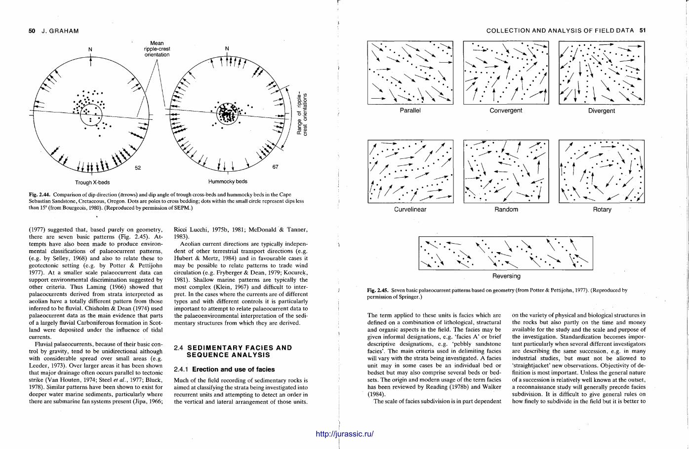
50 J .GRAHAM
Mean ripple-crest orientation
Trough X-beds Hummocky beds
A «
o ®
OJ (D
Fig. 2.44. Comparison of dip direction (arrows) and dip angle of trough cross-beds and hummocky beds in the Cape Sebastian Sandstone, Cretaceous, Oregon. Dots are poles to cross bedding; dots within the small circle represent dips less than 15° (from Bourgeois, 1980). (Reproduced by permission of SEPM.)
(1977) suggested that , based purely on geometry , there are seven basic pat terns (Fig. 2.45). Attempts have also been m a d e to produce environmental classifications of palaeocurrent pat terns , (e.g. by Selley, 1968) and also to relate these to geotectonic setting (e.g. by Pot ter & Petti john 1977). A t a smaller scale palaeocurrent data can support environmental discrimination suggested by other criteria. Thus Laming (1966) showed that palaeocurrents derived from strata interpreted as aeolian have a totally different pat tern from those inferred to be fluvial. Chisholm & D e a n (1974) used palaeocurrent data as the main evidence that parts of a largely fluvial Carboniferous formation in Scotland were deposited under the influence of tidal currents.
Fluvial palaeocurrents , because of their basic control by gravity, tend to be unidirectional al though with considerable spread over small areas (e.g. Leeder , 1973). Over larger areas it has been shown that major drainage often occurs parallel to tectonic strike (Van Hou ten , 1974; Steel e r a / . , 1977; Bluck, 1978). Similar pat terns have been shown to exist for deeper water marine sediments , particularly where there are submarine fan systems present (Jipa, 1966;
Ricci Lucchi, 1975b, 1981; McDonald & Tanner , 1983).
Aeol ian current directions are typically independent of o ther terrestrial t ransport directions (e.g. Hube r t & Mertz , 1984) and in favourable cases it may be possible to relate pat terns to t rade wind circulation (e.g. Fryberger & D e a n , 1979; Kocurek, 1981). Shallow mar ine pat terns are typically the most complex (Klein, 1967) and difficult to interpret . In the cases where the currents are of different types and with different controls it is particularly important to a t tempt to relate palaeocurrent data to the palaeoenvironmental interpretat ion of the sedimentary structures from which they are derived.
2.4 S E D I M E N T A R Y F A C I E S A N D S E Q U E N C E A N A L Y S I S
2.4.1 Erection and use of facies
Much of the field recording of sedimentary rocks is aimed at classifying the strata being investigated into recurrent units and at tempting to detect an order in the vertical and lateral a r rangement of those units.
COLLECTION AND ANALYSIS OF FIELD DATA 51
Parallel Convergent Divergent
Curvelinear Random Rotary
Reversing
Fig. 2.45. Seven basic palaeocurrent patterns based on geometry (from Potter & Pettijohn, 1977). (Reproduced by permission of Springer.)
The term applied to these units is facies which are defined on a combinat ion of lithological, structural and organic aspects in the field. The facies may be given informal designations, e^g. 'facies A ' or brief descriptive designations, e.g. 'pebbly sandstone facies'. The main criteria used in delimiting facies will vary with the strata being investigated. A facies unit may in some cases be an individual bed or bedset but may also comprise several beds or bed-sets. T h e origin and modern usage of the term facies has been reviewed by Reading (1978b) and Walker (1984).
The scale of facies subdivision is in part dependent
on the variety of physical and biological structures in the rocks but also partly on the time and money available for the study and the scale and purpose of the investigation. Standardization becomes important particularly when several different investigators are describing the same succession, e.g. in many industrial studies, but must not be allowed to 'straightjacket ' new observations. Objectivity of definition is most important . Unless the general nature of a succession is relatively well known at the outset , a reconnaissance study will generally precede facies subdivision. It is difficult to give general rules on how finely to subdivide in the field but it is bet ter to
http://jurassic.ru/
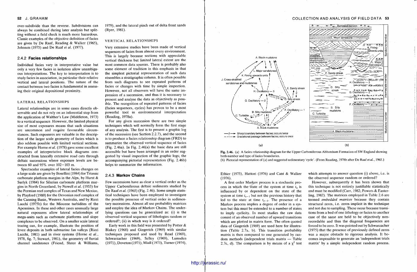
52 J .GRAHAM
over-subdivide than the reverse. Subdivisions can always be combined during later analysis but splitting without a field check is much more hazardous . Classic examples of the objective definition of facies are given by De Raaf, Reading & Walker (1965), Johnson (1975) and D e Raaf et al. (1977).
2.4.2 Facies relat ionships
Individual facies vary in interpretative value but only a very few facies in isolation allow unambiguous interpretat ions. T h e key to interpretat ion is to study facies in association, in particular their relative vertical and lateral positions. The nature of the contact between two facies is fundamental in assessing their original depositional proximity.
L A T E R A L R E L A T I O N S H I P S
Lateral relationships are in some cases directly observable and do not rely on an inferential step from the application of Walther 's Law (Middleton, 1973) to a vertical sequence. However , the limited physical size of most exposures means that such situations are uncommon and require favourable circumstances. Such exposures are valuable in the description of the larger scale geometry of facies which is also seldom possible with limited vertical sections. For example H o m e et al. (1978) gave some excellent examples of interpretative block diagrams constructed from laterally extensive road cuts through deltaic successions where exposure levels are between 60 and 9 5 % over 1 0 2 - 1 0 3 m.
Spectacular examples of lateral facies changes on a large scale are given by Bosellini (1984) for Triassic carbonate platform margins in the Alps , by Hurs t & Surlyk (1984) for Silurian carbonate platform margins in North Greenland , by Newell et al. (1953) for the Permian reef complex of Texas and New Mexico, by Playford (1980) for the Devonian reef complex of the Canning Basin, Western Austral ia, and by Ricci Lucchi (1975b) for the Miocene turbidites of the Apennines . In these and other cases unusually large natural exposures allow lateral relationships of mega-units such as carbonate platforms and slope complexes to be observed. On a smaller scale lateral tracing can, for example , illustrate the position of levee deposits in both submarine fan valleys (Ricci Lucchi, 1981) and in river systems ( H o m e et al., 1978, fig. 7; Stewart , 1981), the geometry of fluvial channel sandstones (Friend, Slater & Williams,
1979), and the lateral pinch out of delta front sands (Ryer , 1981).
V E R T I C A L R E L A T I O N S H I P S
Very extensive studies have been made of vertical sequences of facies from almost every environment . This is largely because sections with appreciable vertical thickness but limited lateral extent are the most common data sources. There is probably also some element of tradition in this emphasis in that the simplest pictorial representat ion of such data resembles a stratigraphic column. It is often possible from such diagrams to see repeated pat terns of facies or changes with t ime by simple inspection. However , not all observers will have the same in> pression of a succession, and thus it is necessary to present and analyse the data as objectively as possible. The recognition of repeated pat terns of facies (facies sequences, cycles) has proven to be a most powerful tool in environmental interpretat ion (Reading, 1978a).
For any given succession there are two simple techniques which will normally form the first stage of any analysis. The first is to present a graphic log of the succession (see Section 2.2.7), and the second is to produce a facies relationship diagram ( F R D ) to summarize the observed vertical sequence of facies (Fig. 2.46a). In Fig. 2.46(a) the basic data are still accessible but have been arranged in an order suggested by visual inspection of the graphic logs; the accompanying pictorial representat ion (Fig. 2.46b) helps to summarize the information.
2.4.3 Markov Chains
Few successions have as clear a vertical order as the Uppe r Carboniferous deltaic sediments studied by D e Raaf etal. (1965) (Fig. 2.46). Some simple statistical techniques have been employed to investigate the possible presence of vertical order in sedimentary successions. Almost all use probability matrices and employ the idea of Markov Chains. The underlying questions can be generalized as: (i) is the observed vertical sequence of lithologies r andom or o rde red? ; (ii) in which way is it o rdered?
Early work in this field was presented by Pot ter & Blakey (1968) and Gingerich (1969) with similar techniques proposed and used by Read (1969), Schwarzacher (1969), Selley (1969), Lumsden (1971), Doveton (1971), Miall (1973), Turner (1974),
COLLECTION AND ANALYSIS OF FIELD DATA 53
A. Black mudstone
\ * K 1 2 \ \
/ ' v * V ,•1 / L . Majorsandstones\\
K. Fining upwards units i J. Cross-stratified sandstones and mudstones
E. Sandy streak
Tl!^\\f • 1 i ~ » T D . S i l t y streak
F. Oscillatory — 1
A. Black mudstone
- 2 — » • Sharp boundary between facies; occurs twice -1 — G r a d a t i o n a l passage between facies; occurs once
. Burrowed horizon
- L Major sandstonez
q o , o . o i o i t , a . o - o b
Q. Oscillatory — 2 _ 9 b ^ 8 ' Q.'s S o - » . D " 0 : ; t O a
e"o: e 6 ' « - e . P o ee.B'.e.e
• B. Silty mudstone
F. Oscillatory— 1:
C. Turbidite
-A. Black mudstone-
(a) (b)
Fig. 2.46. (a) A facies relationship diagram for the Upper Carboniferous Abbotsham Formation of SW England showing both number and type of facies boundaries. (b) Pictorial representation of (a) and suggested sedimentary 'cycle'. (From Reading, 1978b after De Raaf etal., 1965.)
Ethier (1975), Hat tor i (1976) and Cant & Walker (1976).
A first order Markov process is a stochastic process in which the^state of the system at t ime t„ is influenced by or dependent on the state of the system at t ime f„_ { but not the previous history that led to the state at t ime t„-.x. The presence of a Markov process implies a degree of order in a system but this must be extended to a number of states to imply cyclicity. In most studies the raw data consist of an observed number of upward transitions which are plotted in matrix form. The often quoted data of Gingerich (1969) are used here for illustration (Table 2.7a, b ) . This transition probability matrix is then compared to one generated by random methods ( independent trials matrix — Table 2.7c, d) . The comparison is by means of a %2 test
which a t tempts to answer question (i) above, i.e. is the observed sequence random or ordered?
However , subsequently it has been shown that this technique is not entirely justifiable statistically and must be modified (Carr , 1982; Powers & Easter-ling, 1982). The matrices employed in Table 2.6 are te rmed embedded matrices because they contain structural zeros, i.e. zeros implicit in the technique and not due to sampling. These occur because transitions from a bed of one iithology or facies to another case of the same are held to be objectively non-recordable and thus the diagonal frequencies are forced to be zero . It was pointed out by Schwarzacher (1975) that the presence of previously defined zeros was a major obstacle to rigorous analysis. It becomes impossible to generate an ' independent trials matrix ' by a simple independent random process.
http://jurassic.ru/
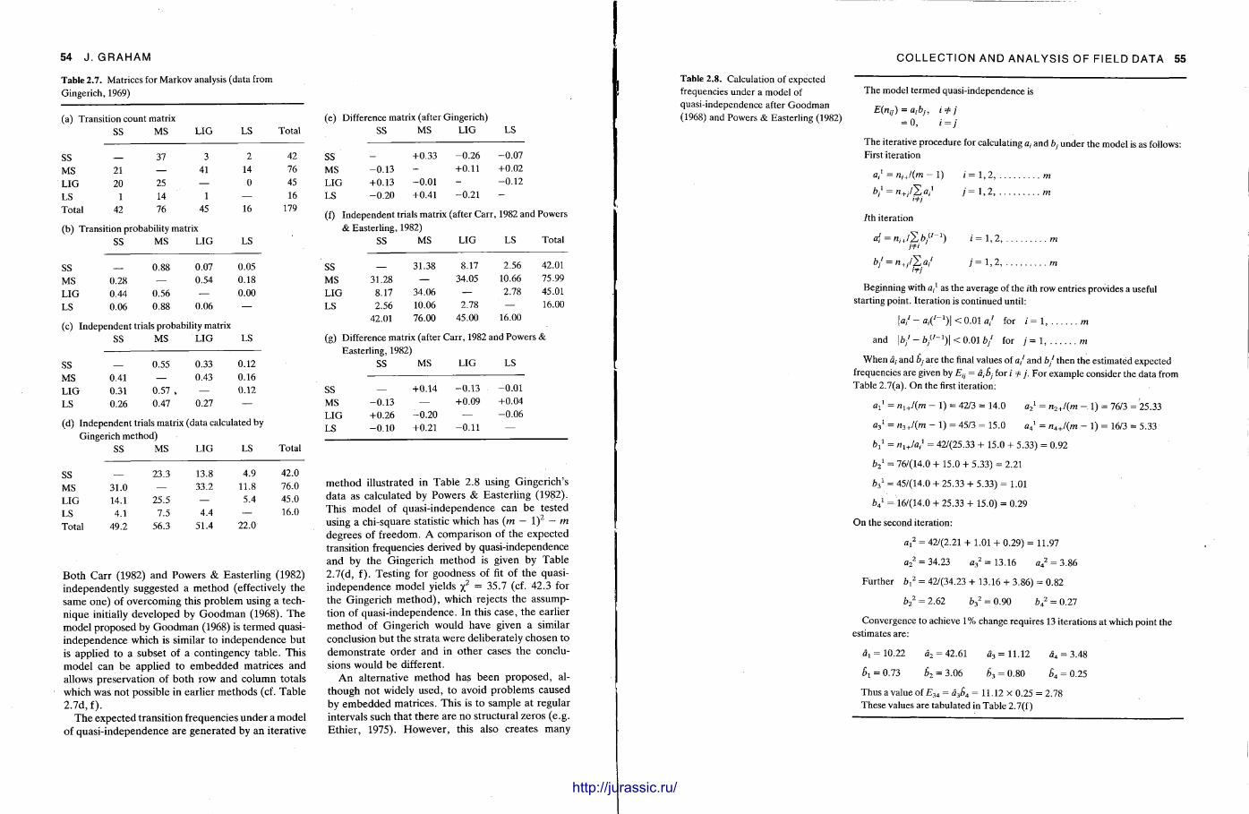
54 J . GRAHAM
Table 2.7. Matrices for Markov analysis (data from Gingerich, 1969)
(a) Transition count matrix SS MS LIG LS Total
SS 37 3 2 42 MS 21 — 41 14 76 LIG 20 25 0 45 LS 1 14 1 — 16 Total 42 76 45 16 179
(b) Transition probability matrix SS MS LIG LS
SS 0.88 0.07 0.05 MS 0.28 — 0.54 0.18 LIG 0.44 0.56 — 0.00 LS 0.06 0.88 0.06
(c) Independent trials probability matrix SS MS LIG 1 S
SS 0.55 0.33 0.12 MS 0.41 — 0.43 0.16 LIG 0.31 0.57 . — 0.12 LS 0.26 0.47 0.27 —
(d) Independent trials matrix (data calculated by Gingerich method)
SS MS LIG LS Total
SS 23.3 13.8 4.9 42.0 MS 31.0 — 33.2 11.8 76.0 LIG 14.1 25.5 — 5.4 45.0 LS 4.1 7.5 4.4 — 16.0 Total 49.2 56.3 51.4 22.0
Both Carr (1982) and Powers & Easterl ing (1982) independent ly suggested a method (effectively the same one) of overcoming this problem using a technique initially developed by G o o d m a n (1968). T h e model proposed by Goodman (1968) is termed quasi-independence which is similar to independence but is applied to a subset of a contingency table. This model can be applied to embedded matrices and allows preservation of both row and column totals which was not possible in earlier methods (cf. Table 2 . 7 d , f ) .
T h e expected transit ion frequencies unde r a model of quasi- independence are generated by an iterative
(e) Difference matrix (after Gingerich) SS MS LIG LS
SS +0.33 -0 .26 -0 .07 MS -0 .13 - +0.11 +0.02 LIG +0.13 -0.01 - -0 .12 LS -0.20 +0.41 -0.21 -(f) Independent trials matrix (after Carr, 1982 and Powers
& Easterling, 1982) SS MS LIG LS Total
SS — 31.38 8.17 2.56 42.01 MS 31.28 — 34.05 10.66 75.99 LIG 8.17 34.06 — 2.78 45.01 LS 2.56 10.06 2.78 — 16.00
42.01 76.00 45.00 16.00
(g) Difference matrix (after Carr, 1982 and Powers & Easterling, 1982)
SS MS LIG LS
SS +0.14 -0 .13 -0 .01 MS -0 .13 — +0.09 +0.04 LIG +0.26 -0.20 — -0 .06 LS -0 .10 +0.21 -0 .11 —
method illustrated in Table 2.8 using Gingerich 's da ta as calculated by Powers & Easterl ing (1982). This model of quasi- independence can be tested using a chi-square statistic which has (m — l ) 2 — m degrees of freedom. A comparison of the expected transition frequencies derived by quasi-independence and by the Gingerich method is given by Table 2.7(d, f ) . Testing for goodness of fit of the quasi-independence model yields %2 = 35.7 (cf. 42.3 for the Gingerich me thod ) , which rejects the assumption of quasi- independence. In this case, the earlier method of Gingerich would have given a similar conclusion but the strata were deliberately chosen to demonst ra te order and in other cases the conclusions would be different.
A n alternative method has been proposed, although not widely used, to avoid problems caused by embedded matrices. This is to sample at regular intervals such that there a r e no structural zeros (e.g. Ethier , 1975). However , this also creates many
mam
COLLECTION AND ANALYSIS OF FIELD DATA 55
Table 2.8. Calculation of expected frequencies under a model of quasi-independence after Goodman (1968) and Powers & Easterling (1982)
The model termed quasi-independence is
E(nu) = aibJ, ii= j = 0, i=j
The iterative procedure for calculating a, and b, under the model is as follows: First iteration
a,' = ni+/(m - 1) i = 1, 2, m
bj1 = n+j/'Zai' y = 1,2, m /th iteration
a? = nij'2bf'-1) i = l , 2 , m b,' = a' 7 = 1 , 2 , m
•f) Beginning with a,1 as the average of the rth row entries provides a useful
starting point. Iteration is continued until: | a / - a ,< / - 1 ) | < 0.01 a / for / = 1, m
and | b / - i » / / _ 1 ) | < 0 . 0 1 b / for y = l , m
When a, and b y are the final values of a/ and b / then the estimated expected frequencies are given by £ / ; = a,b, for i i= j . For example consider the data from Table 2.7(a). On the first iteration:
ai1 = nl+l(m - 1) = 42/3 = 14.0 a2
l = n2+l(m - 1) = 76/3 = 25.33
a 3 ' = n 3 + / (m - 1) = 45/3 = 15.0 a 4 ' = n 4 + / (m - 1) = 16/3 = 5.33
ft,1 = n1+/al = 42/(25.33 + 15.0 + 5.33) = 0.92
b2
1 = 76/(14.0 + 15.0 + 5.33) = 2.21
& 3 1 = 45/(14.0 + 25.33 + 5.33) = 1.01
&41 = 16/(14.0 + 25.33 + 15.0) = 0.29
On the second iteration:
a? = 42/(2.21 + 1.01 + 0.29) = 11.97
a 2
2 = 34.23 a 3
2 = 13.16 a/ = 3.86
Further b , 2 = 42/(34.23 + 13.16 + 3.86) = 0.82
b 2
2 = 2.62 b 3
2 = 0.90 b 4
2 = 0.27
Convergence to achieve 1% change requires 13 iterations at which point the estimates are:
d, = 10.22 d2 = 42.61 a 3 = 11.12 a 4 = 3.48
bi = 0.73 b 2 = 3.06 b 3 = 0.80 b 4 = 0.25
Thus a value of £ 3 4 = a 3 b 4 = 11.12 x 0.25 = 2.78 These values are tabulated in Table 2.7(f)
http://jurassic.ru/

56 J. GRAHAM
problems as the choice of sample interval is very important . The sample interval must be sufficiently small to catch important transitions and this usually leads to large diagonal frequencies with which testing the full matrix for independence can be misleading. This can be overcome by testing off-diagonal frequencies against the model of quasi-independence. In general , there seems to be little advantage in following this more complex method .
Having established that a succession contains some order , the next question concerns the na ture of that order and an identification of preferred transitions (question (ii) above) . Gingerich (1969) a t tempted to express that order by constructing a difference matrix (Table 2.7e) produced by subtracting the independent trials matrix (the 'expected ' results) from the transition probability matrix (the 'observed' results) . A n assumption is made that the positive elements in this matrix have a higher than random chance of occurring. All positive differences are used to indicate the path of the sedimentary 'cycle'. With minor alterations most later workers have employed a similar technique. However , small positive differences can arise from a random process and failure to evaluate the significance of positive differences can lead to the identification of too many preferred transitions (Harper , 1984). Similarly, negative depar tures are ignored by this technique even though they contr ibute to the test statistic and to the rejection of the model of independence .
The currently used techniques for identifying sources of non-randomness are relatively crude and demonst ra te the need for further research. Such techniques involve the identification of ' ex t reme ' cells, i .e. those which show the largest differences between observed and expected transition frequencies. A simple method (Turk, 1979; Powers & Easterl ing, 1982) is to tabulate
Z,j = {Oij - En)IEJn.
The Z,y's are squared and summed to yield %2 and they have approximately the s tandard normal distribution. As 9 5 % of the standard normal distribution falls between ± 2 . 0 , so a ZV] value outside this is fairly unusual . Analysis of the Gingerich data (Table 2.9) shows that the primary contr ibutor to the large X2 is the large number of transitions from lignite to sandstone.
Table 2.9. Normalized differences (0, y - £, y )/£, y " 2
SS MS LIG LS
SS _ + 1.02 -1.81 -0.35 MS -1.84 - + 1.19 + 1.02 LIG +4.14 -1.55 - -1 .67 LS -0.98 + 1.02 -1.07 -
Where 0 / y is shown in Table 2.7(a), £,y is shown in Table 2.7(f).
D — * ~ A — * • Bo B 3 -* - D
D A B 2 ^ B 3 D
B A C
Fig. 2.47. Tree diagrams for Devonian fluvial sediments which show upward facies transition probabilities >0.15. Arbitrary selection of this value is used to imply order of sequence (from Allen, 1970). (Reproduced by permission ofSEPM.)
COLLECTION AND ANALYSIS OF FIELD DATA 57
An alternative method is described by Brown (1974) and Carr (1982). The x2, is calculated for each cell and that whose elimination produces the smallest X2 is deleted, i.e. t reated as a structural zero. The remaining cells are then refitted by a quasi-independent model and the %2 test for quasi- independence is recalculated. This stepwise procedure is continued until a chosen level of significance. Correct identification of a single cell when it is the only cell that does not fit a quasi- independent model is a far simpler problem than identifying a subset of cells, all of which deviate from a model fitted to the other cells. An optimal solution to this latter problem has yet to be found but all ext reme cells are likely to be identified. In the case of the Gingerich data , a chosen level of significance of a = 0.1 was exceeded after selection of the first cell (sandstone over ligni te) . This shows good agreement with the normalized differences approach above.
grams. Their aim is to present either the raw data or statistics based on those da ta in a format which aids interpretat ion. Figure 2.46(a) above was derived from the raw data and retained information on the na ture of facies boundar ies as well as number of transitions. O the r workers have a t tempted to select from the raw data the more commonly occurring transitions (e.g. Allen, 1970 and Fig. 2.47), in some cases implying preferred sequence.
Preferred sequence has been suggested mainly following statistical analysis of data , usually by plotting the positive elements of the difference matrix (Gingerich, 1969; Miall, 1973; Hube r t & Hyde , 1982) (Figs 2.48, 2.49 and 2.50). The data of Gingerich
Sandstone ^Mudstone *• Lignite
D A T A P R E S E N T A T I O N A N D I N T E R P R E T A T I O N
Vertical a r rangement of different facies can be represented by a variety of facies relationship dia-
Limestone
Fig. 2.48. Tree diagram constructed from the positive elements of the differences matrix (Table 2.8d) (after Gingerich, 1969). (Reproduced by permission of SEPM.)
Difference matrix, Lower Peel Sound Formation
Fig. 2.49. Difference matrix 1 2 3 4 5 6 7
constructed for Devonian fluvial sediments, Arctic Canada, following Conglomerate 1 0.00 0.25 0.02 0.02 -0 .06 -0.09 -0.14 the methodology of Gingerich (1969). Red sandstone 2 0.33 0.00 -0 .03 -0.01 -0.20 -0 .06 -0.02 The accompanying tree diagram Red siltstone 3 0.19 -0 .23 0.00 -0.01 0.01 0.16 -0 .13 distinguishes between 'major' Red limestone 4 0.20 -0 .23 -0 .02 0.00 -0.23 0.41 -0.13 =d,j transition paths (solid lines) and Grey sandstone 5 0.03 -0.15 0.00 -0.01 0.00 0.07 0.07 'minor' transition paths (dashed lines). Grey siltstone 6 -0 .20 -0 .12 -0 .02 -0.01 0.25 0.00 0.11 on the basis of values in the difference Grey limestone 7 -0.21 -0.17 -0 .02 -0 .01 0.39 0.03 0.00 matrix (from Miall, 1973).
Grey limestone
http://jurassic.ru/
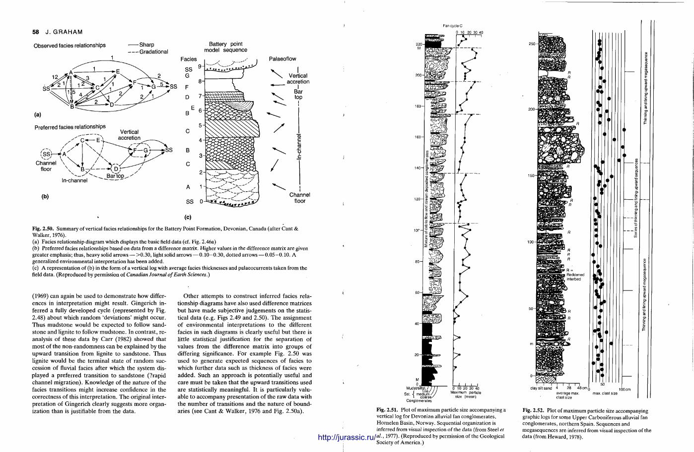
58 J . GRAHAM
Observed facies relationships —Sharp — Gradational
Preferred facies relationships
fssj— Channel
floor
Vertical accretion
In-channel
(b)
Battery point model sequence
Facies
S S G
F
D
B
C
A
S S
(c)
Palaeoflow
V 1
\ Vertical accretion
Bar top
i
/
CD C CO o c
Channel floor
Fig. 2.50. Summary of vertical facies relationships for the Battery Point Formation, Devonian, Canada (after Cant & Walker, 1976). (a) Facies relationship diagram which displays the basic field data (cf. Fig. 2.46a) (b) Preferred facies relationships based on data from a difference matrix. Higher values in the difference matrix are given greater emphasis; thus, heavy solid arrows — >0.30, light solid arrows — 0.10—0.30, dotted arrows — 0.05-0.10. A generalized environmental interpretation has been added. (c) A representation of (b) in the form of a vertical log with average facies thicknesses and palaeocurrents taken from the field data. (Reproduced by permission of Canadian Journal of Earth Sciences.)
(1969) can again be used to demonst ra te how differences in interpretat ion might result. Gingerich inferred a fully developed cycle (represented by Fig. 2.48) about which random 'deviations' might occur. Thus mudstone would be expected to follow sandstone and lignite to follow mudstone . In contrast , re-analysis of these data by Carr (1982) showed that most of the non-randomness can be explained by the upward transition from lignite to sandstone. Thus lignite would be the terminal state of r andom succession of fluvial facies after which the system displayed a preferred transition to sandstone (?rapid channel migrat ion) . Knowledge of the na ture of the facies transitions might increase confidence in the correctness of this interpretat ion. The original interpretat ion of Gingerich clearly suggests more organization than is justifiable from the data .
Other at tempts to construct inferred facies relationship diagrams have also used difference matrices but have made subjective judgements on the statistical data (e.g. Figs 2.49 and 2.50). T h e assignment of environmental interpretat ions to the different facies in such diagrams is clearly useful but there is little statistical justification for the separat ion of values from the difference matrix into groups of differing significance. For example Fig. 2.50 was used to generate expected sequences of facies to which further data such as thickness of facies were added. Such an approach is potentially useful and care must be taken that the upward transitions used are statistically meaningful. It is particularly valuable to accompany presentat ion of the raw data with the number of transitions and the na ture of boundaries (see Cant & Walker , 1976 and Fig. 2.50a).
F a n c y c l e C
C o n g l o m e r a t e s
Fig. 2.51. Plot of maximum particle size accompanying a Fig. 2.52. Plot of maximum particle size accompanying vertical log for Devonian alluvial fan conglomerates, graphic logs for some Upper Carboniferous alluvial fan Hornelen Basin, Norway. Sequential organization is conglomerates, northern Spain. Sequences and inferred from visual inspection of the data (from Steel et megasequences are inferred from visual inspection of the al., 1977). (Reproduced by permission of the Geological data (from Heward, 1978). Society of America.)
i l l l l M http://jurassic.ru/
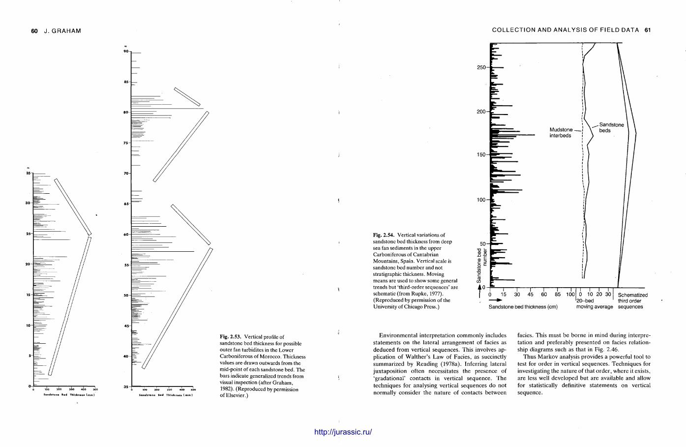
60 J. GRAHAM
200 300 400
Sandstone Bed Th ickness ( n
200 300 400 500
S a n d s t o n e Bed Th Ick ness t m m )
Fig. 2.53. Vertical profile of sandstone bed thickness for possible outer fan turbidites in the Lower Carboniferous of Morocco. Thickness values are drawn outwards from the mid-point of each sandstone bed. The bars indicate generalized trends from visual inspection (after Graham, 1982). (Reproduced by permission of Elsevier.)
COLLECTION AND ANALYSIS OF FIELD DATA 61
Fig. 2.54. Vertical variations of sandstone bed thickness from deep sea fan sediments in the upper Carboniferous of Cantabrian Mountains, Spain. Vertical scale is sandstone bed number and not stratigraphic thickness. Moving means are used to show some general trends but 'third-order sequences' are schematic (from Rupke, 1977). (Reproduced by permission of the University of Chicago Press.) Sandstone bed thickness (cm) moving average sequences
Environmenta l interpretat ion commonly includes s tatements on the lateral ar rangement of facies as deduced from vertical sequences. This involves application of Walther ' s Law of Facies, as succinctly summarized by Reading (1978a). Inferring lateral juxtaposit ion often necessitates the presence of 'gradational ' contacts in vertical sequence. The techniques for analysing vertical sequences do not normally consider the nature of contacts between
facies. This must be borne in mind during interpretation and preferably presented on facies relationship diagrams such as that in Fig. 2.46.
Thus Markov analysis provides a powerful tool to test for order in vertical sequences. Techniques for investigating the na ture of that order , where it exists, are less well developed but are available and allow for statistically definitive s tatements on vertical sequence.
http://jurassic.ru/
62 J . GRAHAM
2.4.4 Non-Markov techniques for sequence analysis
Presentat ion and analysis of vertical sequences of rock is not limited to Markov analysis. Several o ther , often simpler, techniques have been employed with considerable success. Perhaps the most common are those that consider vertical changes in grain size or bed thickness. T h e former have commonly been employed in the study of conglomerates (Figs 2.24c, 2.51 and 2.52) (Bluck, 1967; Steel etal., 1977; Heward , 1978; Surlyk, 1978; Allen, 1981). T h e aim has largely been the detection of sequences showing a unidirectional variation of maximum clast size, i.e. coarsening up (CU) or fining up (FU) sequences. The detection of such sequences has often been by simple visual inspection of the data but they are also susceptible to techniques such as moving means .
Vertical changes in layer thickness have also been
useful, particularly in turbidite successions (Ricci Lucchi, 1975b; R u p k e , 1977; Shanmugam, 1980; G r a h a m , 1982). Techniques of presentat ion show considerable variation, e.g. the vertical scale may be stratigraphic thickness as in Fig. 2.53 or sandstone number as in Fig. 2.54. A criticism of many of these presentat ions is that ' t rends ' are designated from visual inspection of the data (Fig. 2 .53, Fig. 2.54 — third order sequences) without any statistical justification. Techniques such as moving means (Fig. 2.54) can be useful here although these should always be presented along with the original da ta as averaging will lead to displacement of the peak values that are commonly used to delimit packets of sediment (rhythms or cycles). O n e must take care that compared units of thickness have similar definition and that their significance is unders tood (see Section 2.2.3).
3 Grain size determination and interpretation JOHN MCMANUS
3.1 I N T R O D U C T I O N
The size of the component particles is one of the fundamental textural characteristics of all fragmentary deposits and their lithified equivalents. From the earliest days of observation and recording of geological features, terms such as 'coarse ' , 'medium' or 'fine' grained have been applied to unconsolidated deposits . Al though considered a useful lithological discriminator for tracing individual horizons during geological mapping, little systematic study of grain size characterization and measurement occurred before the end of the nineteenth century. By that t ime there was already an appreciation that very substantial currents of water were necessary to transport coarse sediments but , without systematic means of establishing precisely the sizes of particles and the range of particle sizes within a deposit , little scientific advance was made .
In general terms, 'size' of particles is not readily defined as it is a measure of the dimensions which best describe a specific group of particles. At one ext reme the particle dimensions may exceed one me t re , but at the other are the very fine particles less than one micrometre in diameter . A cube may be best described by its edge length, a sphere by its d iameter , a rod perhaps by its intermediate axis and a flake by its projection area. Thus 'size' is partly dependent on shape , a fact which was gradually recognized during the early years of the present century.
T h e methods used in determinat ion of size vary widely from calipers on the coarsest fragments, through sieving and techniques dependent upon settling velocity, to those detecting changes in electrical resistance as particles are passed through small electrolyte-filled orifices. N o single technique of assessing particle size is applicable throughout the entire size spectrum, and each is suited to specific size ranges.
Al though when measuring pebbles to determine axial lengths individually, relatively small numbers of grains are considered, in most methods large
numbers of grains are examined so that a statistically meaningful set of numbers is obtained to characterize the sample.
T h e techniques of processing the data on grain size were largely explored during the 1920s and 1930s when a series textural classifications was int roduced. In their simplest forms these classifications indicate average grain size, and the degree and form of the spread around that average. Statistical analysis is aided by means of a simple transformation of size from a metric scale to a logarithmic one which enables application of both graphic and moment statistical techniques. Explored initially for sand-dominated assemblages, the methods were refined during the 1950s and applied to thin section analysis of lithified sediments during the early 1960s. Fresh techniques of exploring the information on grain populations with a view to interpreting depositional environment or t ransporta t ion experienced by the deposits continue to be introduced with varying degrees of success. Many have appeared, been explored and found applicable only under certain restricted conditions.
E v e n t h e most sanguine grain size enthusiast would agree that no universal solution exists as yet to enable the sedimentologist unequivocally to distinguish depositional environments in ancient deposits on grain size criteria a lone. Nevertheless, an enormous amount of information about a sedimentary deposit may be obtained from systematic examination of the multiple sub-populations of which most are formed. Specific sub-populations may be source-or process-diagnostic, a factor which frequently emerges from regional surveys.
From the outset it is most important that the investigator should decide precisely what information is required from the sediments to be analysed (McCave, 1979a). Analysis solely to obtain numerical assessment of the texture of a deposit is unlikely to satisfy the sedimentologist but this information may be all that is required to demonst ra te to a fisheries expert the potential value of a site for the introduction of an economically important species
6 3
http://jurassic.ru/
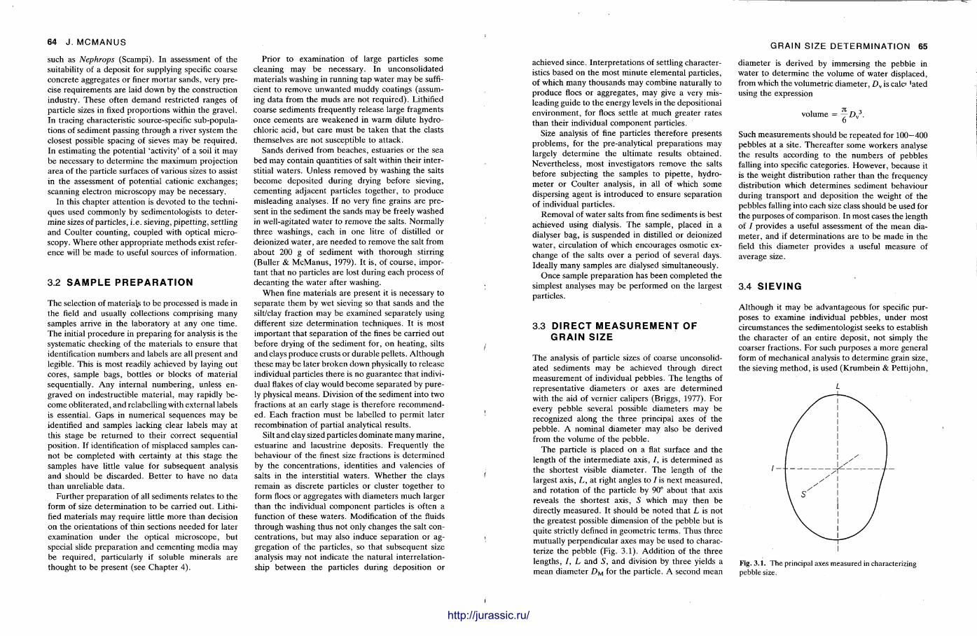
64 J. MCMANUS
such as Nephrops (Scampi). In assessment of the suitability of a deposit for supplying specific coarse concrete aggregates or finer mor tar sands, very precise requirements are laid down by the construction industry. These often demand restricted ranges of particle sizes in fixed proport ions within the gravel. In tracing characteristic source-specific sub-populations of sediment passing through a river system the closest possible spacing of sieves may be required. In estimating the potential 'activity' of a soil it may be necessary to determine the maximum projection area of the particle surfaces of various sizes to assist in the assessment of potential cationic exchanges; scanning electron microscopy may be necessary.
In this chapter at tention is devoted to the techniques used commonly by sedimentologists to determine sizes of particles, i.e. sieving, pipett ing, settling and Coulter counting, coupled with optical microscopy. W h e r e other appropr ia te methods exist reference will be made to useful sources of information.
3.2 S A M P L E P R E P A R A T I O N
The selection of materials to be processed is made in the field and usually collections comprising many samples arrive in the laboratory at any one t ime. The initial procedure in preparing for analysis is the systematic checking of the materials to ensure that identification numbers and labels are all present and legible. This is most readily achieved by laying out cores, sample bags, bott les or blocks of material sequentially. Any internal number ing , unless engraved on indestructible material , may rapidly become obli terated, and relabelling with external labels is essential. Gaps in numerical sequences may be identified and samples lacking clear labels may at this stage be re turned to their correct sequential position. If identification of misplaced samples cannot be completed with certainty at this stage the samples have little value for subsequent analysis and should be discarded. Bet ter to have no data than unreliable data .
Fur ther preparat ion of all sediments relates to the form of size determinat ion to be carried out . Lithified materials may require little more than decision on the orientations of thin sections needed for later examination under the optical microscope, but special slide preparat ion and cementing media may be required, particularly if soluble minerals are thought to be present (see Chapter 4) .
Prior to examination of large particles some cleaning may be necessary. In unconsolidated materials washing in running tap water may be sufficient to remove unwanted muddy coatings (assuming data from the muds are not required) . Lithified coarse sediments frequently release large fragments once cements are weakened in warm dilute hydrochloric acid, but care must be taken that the clasts themselves are not susceptible to attack.
Sands derived from beaches , estuaries or the sea bed may contain quantit ies of salt within their interstitial waters . Unless removed by washing the salts become deposited during drying before sieving, cementing adjacent particles together , to produce misleading analyses. If no very fine grains are present in the sediment the sands may be freely washed in well-agitated water to remove the salts. Normally three washings, each in one litre of distilled or deionized water , are needed to remove the salt from about 200 g of sediment with thorough stirring (Buller & McManus , 1979). It is, of course , important that no particles are lost during each process of decanting the water after washing.
When fine materials are present it is necessary to separate them by wet sieving so that sands and the silt/clay fraction may be examined separately using different size determinat ion techniques. It is most important that separat ion of the fines be carried out before drying of the sediment for, on heat ing, silts and clays produce crusts or durable pellets. Al though these may be later broken down physically to release individual particles there is no guarantee that individual flakes of clay would become separated by purely physical means . Division of the sediment into two fractions at an early stage is therefore recommended. Each fraction must be labelled to permit later recombinat ion of partial analytical results.
Silt and clay sized particles dominate many mar ine , estuarine and lacustrine deposits. Frequent ly the behaviour of the finest size fractions is de termined by the concentrat ions, identities and valencies of salts in the interstitial waters . Whe the r the clays remain as discrete particles or cluster together to form floes or aggregates with diameters much larger than the individual component particles is often a function of these waters . Modification of the fluids through washing thus not only changes the salt concentrat ions, but may also induce separat ion or aggregation of the particles, so that subsequent size analysis may not indicate the natural interrelationship between the particles during deposition or
I
1 11111 F
GRAIN SIZE DETERMINATION 65
achieved since. Interpretat ions of settling characteristics based on the most minute elemental particles, of which many thousands may combine naturally to produce floes or aggregates, may give a very misleading guide to the energy levels in the depositional environment , for floes settle at much greater rates than their individual component particles.
Size analysis of fine particles therefore presents problems, for the pre-analytical preparat ions may largely determine the ult imate results obtained. Nevertheless , most investigators remove the salts before subjecting the samples to pipet te , hydrometer or Coul ter analysis, in all of which some dispersing agent is introduced to ensure separation of individual particles.
Removal of water salts from fine sediments is best achieved using dialysis. The sample, placed in a dialyser bag, is suspended in distilled or deionized water , circulation of which encourages osmotic exchange of the salts over a period of several days. Ideally many samples are dialysed simultaneously.
Once sample prepara t ion has been completed the simplest analyses may be performed on the largest particles.
3.3 D I R E C T M E A S U R E M E N T OF G R A I N S I Z E
The analysis of particle sizes of coarse unconsolidated sediments may be achieved through direct measurement of individual pebbles. The lengths of representat ive diameters or axes are determined with the aid of vernier calipers (Briggs, 1977). For every pebble several possible diameters may be recognized along the three principal axes of the pebble . A nominal d iameter may also be derived from the volume of the pebble .
The particle is placed on a flat surface and the length of the intermediate axis, / , is de termined as the shortest visible diameter . The length of the largest axis, L , at right angles to / is next measured, and rotat ion of the particle by 90° about that axis reveals the shortest axis, S which may then be directly measured. It should be noted that L is not the greatest possible dimension of the pebble but is quite strictly defined in geometric terms. Thus three mutually perpendicular axes may be used to characterize the pebble (Fig. 3.1). Addit ion of the three lengths, / , L and 5 , and division by three yields a mean diameter DM for the particle. A second mean
diameter is derived by immersing the pebble in water to determine the volume of water displaced, from which the volumetric diameter , D v is ca lc 'ated using the expression
volume = ^ r D v
3 . 6
Such measurements should be repeated for 100 -400 pebbles at a site. Thereafter some workers analyse the results according to the numbers of pebbles falling into specific categories. However , because it is the weight distribution rather than the frequency distribution which determines sediment behaviour during transport and deposition the weight of the pebbles falling into each size class should be used for the purposes of comparison. In most cases the length of / provides a useful assessment of the mean diameter , and if determinat ions are to be made in the field this diameter provides a useful measure of average size.
3.4 S I E V I N G
Although it may be advantageous for specific purposes to examine individual pebbles , under most circumstances the sedimentologist seeks to establish the character of an entire deposit , not simply the coarser fractions. For such purposes a more general form of mechanical analysis to determine grain size, the sieving method , is used (Krumbein & Pett i john,
L
I
Fig. 3.1. The principal axes measured in characterizing pebble size.
http://jurassic.ru/
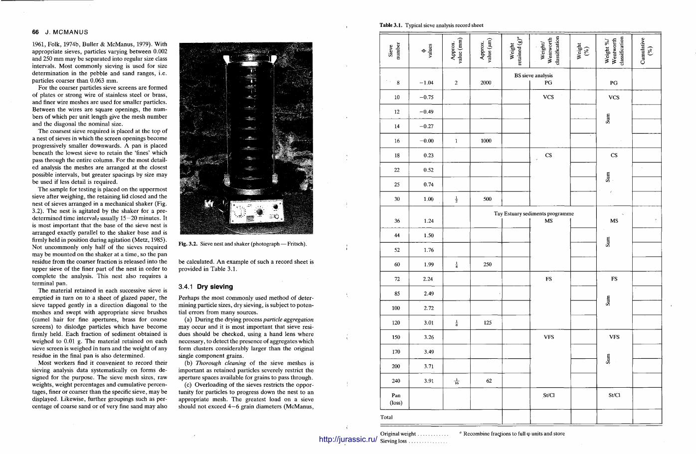
66 J . MCMANUS
1961, Folk, 1974b, Buller & McManus , 1979). With appropr ia te sieves, particles varying between 0.002 and 250 m m may be separated into regular size class intervals. Most commonly sieving is used for size determinat ion in the pebble and sand ranges, i.e. particles coarser than 0.063 mm.
For the coarser particles sieve screens are formed of plates or strong wire of stainless steel or brass, and finer wire meshes are used for smaller particles. Between the wires are square openings, the numbers of which per unit length give the mesh number and the diagonal the nominal size.
The coarsest sieve required is placed at the top of a nest of sieves in which the screen openings become progressively smaller downwards . A pan is placed benea th the lowest sieve to retain the 'fines' which pass through the entire column. For the most detailed analysis the meshes are arranged at the closest possible intervals, but greater spacings by size may be used if less detail is required.
The sample for testing is placed on the uppermost sieve after weighing, the retaining lid closed and the nest of sieves arranged in a mechanical shaker (Fig. 3.2). The nest is agitated by the shaker for a predetermined t ime interval? usually 15—20 minutes . It is most important that the base of the sieve nest is arranged exactly parallel to the shaker base and is firmly held in position during agitation (Metz , 1985). Not uncommonly only half of the sieves required may be mounted on the shaker at a t ime, so the pan residue from the coarser fraction is released into the upper sieve of the finer part of the nest in order to complete the analysis. This nest also requires a terminal pan.
T h e material retained in each successive sieve is emptied in turn on to a sheet of glazed paper , the sieve tapped gently in a direction diagonal to the meshes and swept with appropr ia te sieve brushes (camel hair for fine aper tures , brass for coarse screens) to dislodge particles which have become firmly held. Each fraction of sediment obtained is weighed to 0.01 g. The material retained on each sieve screen is weighed in turn and the weight of any residue in the final pan is also determined.
Most workers find it convenient to record their sieving analysis data systematically on forms designed for the purpose . The sieve mesh sizes, raw weights, weight percentages and cumulative percentages, finer or coarser than the specific sieve, may be displayed. Likewise, further groupings such as percentage of coarse sand or of very fine sand may also
Fig. 3.2. Sieve nest and shaker (photograph — Fritsch).
be calculated. A n example of such a record sheet is provided in Table 3 .1 .
3.4.1 Dry sieving
Perhaps the most commonly used method of determining particle sizes, dry sieving, is subject to potential errors from many sources.
(a) Dur ing the drying process particle aggregation may occur and it is most important that sieve residues should be checked, using a hand lens where necessary, to detect the presence of aggregates which form clusters considerably larger than the original single component grains.
(b) Thorough cleaning of the sieve meshes is important as retained particles severely restrict the aper ture spaces available for grains to pass through.
(c) Overloading of the sieves restricts the opportunity for particles to progress down the nest to an appropr ia te mesh. The greatest load on a sieve should not exceed 4—6 grain diameters (McManus ,
(I || |̂ y a ^ ̂^̂̂^̂̂^̂̂^̂̂^̂̂^ ^
Table 3.1. Typical sieve analysis record sheet
Siev
e nu
mbe
r
<t> va
lues
App
rox.
va
lue
(mm
)
App
rox.
va
lue
(urn
)
Wei
ght
reta
ined
(g)
°
Wei
ght/
Weh
twor
th
clas
sific
atio
n
.2?
Wei
ght
%/
Wen
twor
th
clas
sific
atio
n
Cum
ulat
ive
(%)
8 -1 .04 2 2000 BS sie\ ie. analysis
PG PG
10 -0.75 VCS VCS
E 3 oo
12 -0.49
VCS
E 3 oo
14 -0 .27
VCS
E 3 oo
16 -0.00 1 1000
VCS
E 3 oo
18 0.23 CS CS
E 3 00 •
22 0.52
CS
E 3 00 • 25 0.74
CS
E 3 00 •
30 1.00 i 2
500
CS
E 3 00 •
36 1.24 Ta> Estuary sec iments programrr
MS e
MS
E 3 on
44 1.50
MS
E 3 on 52 1.76
MS
E 3 on
60 1.99 1 4 250
MS
E 3 on
72 2.24 FS FS
E 3 on
85 2.49
FS
E 3 on 100 2.72
FS
E 3 on
120 3.01 1 8
125
FS
E 3 on
150 3.26 VFS VFS
E 3 on
170 3.49
VFS
E 3 on
200 3.71
VFS
E 3 on
240 3.91 1 16
62
VFS
E 3 on
Pan (loss)
St/Cl St/Cl
Total
Original weight Sieving loss . . .
" Recombine fractions to full cp units and store http://jurassic.ru/
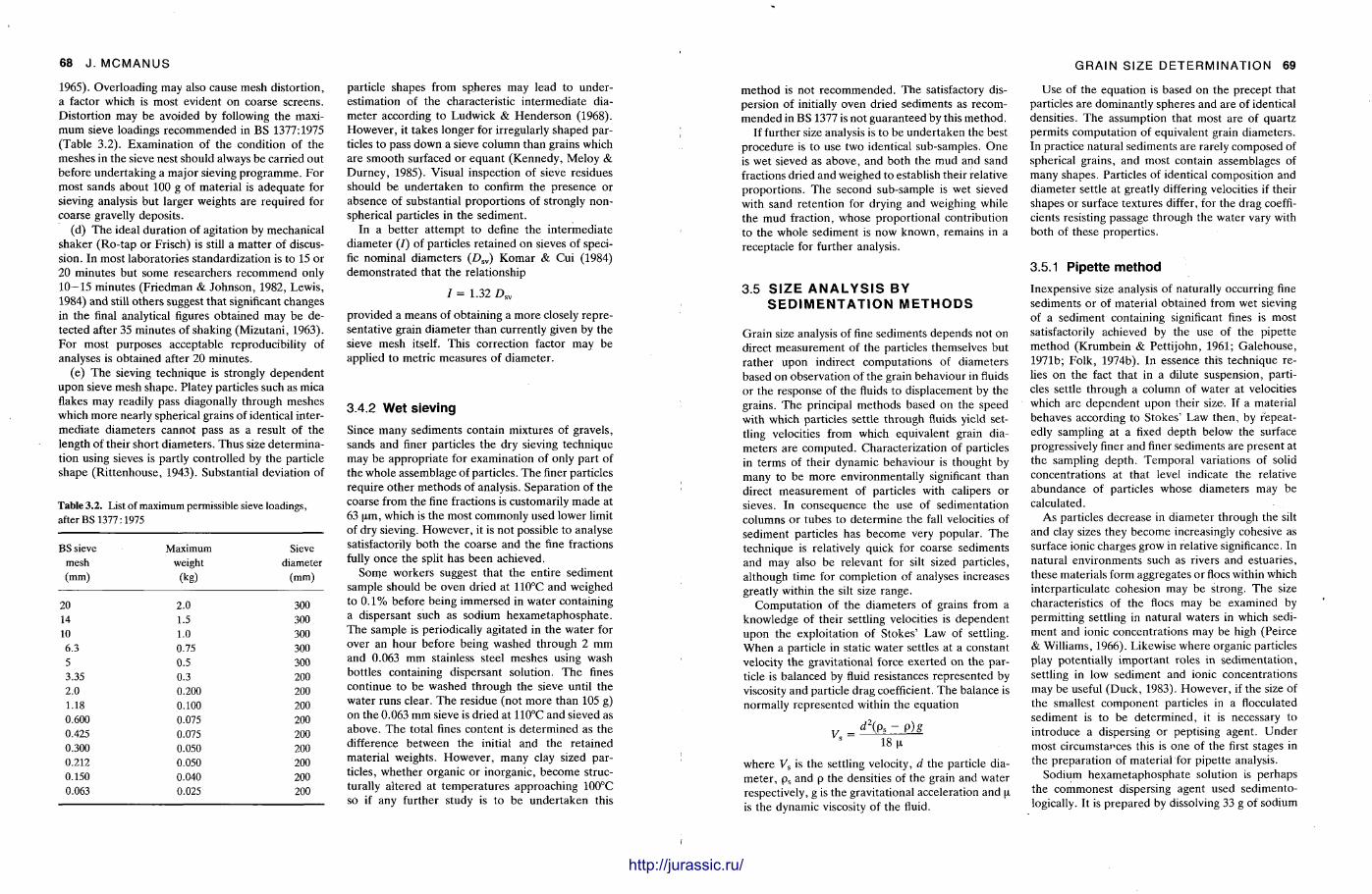
68 J . MCMANUS
1965). Overloading may also cause mesh distortion, a factor which is most evident on coarse screens. Distortion may be avoided by following the maximum sieve loadings recommended in BS 1377:1975 (Table 3.2). Examinat ion of the condition of the meshes in the sieve nest should always be carried out before undertaking a major sieving p rogramme. For most sands about 100 g of material is adequate for sieving analysis but larger weights are required for coarse gravelly deposits.
(d) The ideal durat ion of agitation by mechanical shaker (Ro-tap or Frisch) is still a mat ter of discussion. In most laboratories standardization is to 15 or 20 minutes but some researchers recommend only 10—15 minutes (Fr iedman & Johnson, 1982, Lewis, 1984) and still others suggest that significant changes in the final analytical figures obtained may be detected after 35 minutes of shaking (Mizutani , 1963). For most purposes acceptable reproducibility of analyses is obtained after 20 minutes.
(e) The sieving technique is strongly dependent upon sieve mesh shape. Platey particles such as mica flakes may readily pass diagonally through meshes which more nearly spherical grains of identical intermedia te diameters cannot pass as a result of the length of their short d iameters . Thus size determination using sieves is partly controlled by the particle shape (Ri t tenhouse , 1943). Substantial deviation of
Table 3.2. List of maximum permissible sieve loadings, after BS 1377:1975
BS sieve Maximum Sieve mesh weight diameter (mm) (kg) (mm)
20 2.0 300 14 1.5 300 10 1.0 300 6.3 0.75 300 5 0.5 300 3.35 0.3 200 2.0 0.200 200 1.18 0.100 200 0.600 0.075 200 0.425 0.075 200 0.300 0.050 200 0.212 0.050 200 0.150 0.040 200 0.063 0.025 200
particle shapes from spheres may lead to underestimation of the characteristic intermediate diameter according to Ludwick & Henderson (1968). However , it takes longer for irregularly shaped particles to pass down a sieve column than grains which are smooth surfaced or equant (Kennedy, Meloy & Durney , 1985). Visual inspection of sieve residues should be under taken to confirm the presence or absence of substantial proport ions of strongly non-spherical particles in the sediment.
In a better a t tempt to define the intermediate diameter (I) of particles retained on sieves of specific nominal diameters (£> s v) Komar & Cui (1984) demonst ra ted that the relationship
/ = 1.32 Dsv
provided a means of obtaining a more closely representative grain diameter than currently given by the sieve mesh itself. This correction factor may be applied to metric measures of diameter .
3.4.2 Wet sieving
Since many sediments contain mixtures of gravels, sands and finer particles the dry sieving technique may be appropria te for examination of only part of the whole assemblage of particles. The finer particles require o ther methods of analysis. Separat ion of the coarse from the fine fractions is customarily m a d e at 63 urn, which is the most commonly used lower limit of dry sieving. However , it is not possible to analyse satisfactorily both the coarse and the fine fractions fully once the split has been achieved.
Some workers suggest that the entire sediment sample should be oven dried at 110°C and weighed to 0 . 1 % before being immersed in water containing a dispersant such as sodium hexametaphosphate . The sample is periodically agitated in the water for over an hour before being washed through 2 mm and 0.063 mm stainless steel meshes using wash bottles containing dispersant solution. T h e fines continue to be washed through the sieve until the water runs clear. The residue (not more than 105 g) on the 0.063 mm sieve is dried at 110°C and sieved as above. T h e total fines content is determined as the difference between the initial and the retained material weights. However , many clay sized particles, whether organic or inorganic, become structurally altered at t empera tures approaching 100°C so if any further study is to be under taken this
GRAIN SIZE DETERMINATION 69
method is not r ecommended . The satisfactory dispersion of initially oven dried sediments as recommended in BS 1 3 7 7 is not guaranteed by this method .
If further size analysis is to be under taken the best procedure is to use two identical sub-samples. O n e is wet sieved as above, and both the mud and sand fractions dried and weighed to establish their relative proport ions . The second sub-sample is wet sieved with sand retention for drying and weighing while the mud fraction, whose proport ional contribution to the whole sediment is now known, remains in a receptacle for further analysis.
3.5 S I Z E A N A L Y S I S BY S E D I M E N T A T I O N M E T H O D S
Grain size analysis of fine sediments depends not on direct measurement of the particles themselves but ra ther upon indirect computat ions of diameters based on observation of the grain behaviour in fluids or the response of the fluids to displacement by the grains. T h e principal methods based on the speed with which particles settle through fluids yield settling velocities from which equivalent grain diameters are computed . Characterization of particles in terms of their dynamic behaviour is thought by many to be more environmentally significant than direct measurement of particles with calipers or sieves. In consequence the use of sedimentat ion columns or tubes to determine the fall velocities of sediment particles has become very popular . The technique is relatively quick for coarse sediments and may also be relevant for silt sized particles, al though t ime for completion of analyses increases greatly within the silt size range.
Computa t ion of the diameters of grains from a knowledge of their settling velocities is dependent upon the exploitation of Stokes ' Law of settling. When a particle in static water settles at a constant velocity the gravitational force exerted on the particle is balanced by fluid resistances represented by viscosity and particle drag coefficient. The balance is normally represented within the equat ion
d2(ps - p ) g
1 8 M-
where V s is the settling velocity, d the particle diameter , p s and p the densities of the grain and water respectively, g is the gravitational acceleration and u, is the dynamic viscosity of the fluid.
Use of the equat ion is based on the precept that particles are dominantly spheres and are of identical densities. The assumption that most are of quartz permits computat ion of equivalent grain diameters . In practice natural sediments are rarely composed of spherical grains, and most contain assemblages of many shapes. Particles of identical composition and diameter settle at greatly differing velocities if their shapes or surface textures differ, for the drag coefficients resisting passage through the water vary with both of these propert ies .
3.5.1 Pipette method
Inexpensive size analysis of naturally occurring fine sediments or of material obtained from wet sieving of a sediment containing significant fines is most satisfactorily achieved by the use of the pipette method (Krumbein & Pett i john, 1961; Galehouse , 1971b; Folk, 1974b). In essence this technique relies on the fact that in a dilute suspension, particles settle through a column of water at velocities which are dependent upon their size. If a material behaves according to Stokes ' Law then , by repeatedly sampling at a fixed depth below the surface progressively finer and finer sediments are present at the sampling depth . Tempora l variations of solid concentrat ions at that level indicate the relative abundance of particles whose diameters may be calculated.
As particles decrease in diameter through the silt and clay sizes they become increasingly cohesive as surface ionic charges grow in relative significance. In natural environments such as rivers and estuaries, these materials form aggregates or floes within which interparticulate cohesion may be strong. The size characteristics of the floes may be examined by permit t ing settling in natural waters in which sediment and ionic concentrat ions may be high (Peirce & Williams, 1966). Likewise where organic particles play potentially important roles in sedimentat ion, settling in low sediment and ionic concentrations may be useful (Duck, 1983). However , if the size of the smallest component particles in a flocculated sediment is to be de termined, it is necessary to introduce a dispersing or peptising agent. Under most circumstances this is one of the first stages in the preparat ion of material for pipette analysis.
Sodium hexametaphosphate solution is perhaps the commonest dispersing agent used sedimento-logically. It is prepared by dissolving 33 g of sodium
http://jurassic.ru/
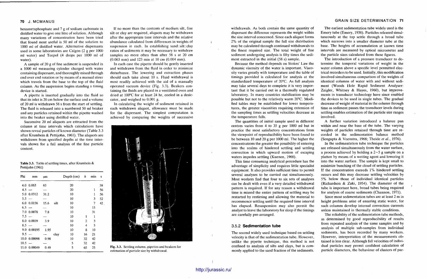
70 J . MCMANUS
hexametaphosphate and 7 g of sodium carbonate in distilled water to give one litre of solution. Although many variations of concentration have been tried that found most useful is 50 ml of the solution to 1000 ml of distilled water . Alternat ive dispersants used in some laboratories are Calgon (2 g per 1000 ml water) and Teepol (4 drops per 1000 ml of water) .
A sample of 20 g of fine sediment is suspended in a 1000 ml measuring cylinder charged with water containing dispersant, and thoroughly mixed through end over end rotation or by means of a manual stirer which travels from the base to the top of the fluid column. As the suspension begins standing a timing device is started.
A pipette is inserted gradually into the fluid so that its inlet is 20 cm below the surface and a volume of 20 ml is withdrawn 58 s from the start of settling. T h e fluid is released into a numbered 50 ml beaker and any particles retained within the pipet te washed into the beaker using distilled water .
Successive 20 ml aliquots are extracted from the column at time intervals which calculations have shown reveal particles of known diameter (Table 3.3 after Krumbein & Pett i john, 1961). The aliquots are withdrawn from specified depths at the t ime intervals shown for a full analysis of the fine particle content .
Table 3 . 3 . Table of settling times, after Krumbein & Pettijohn (1961)
Phi mm urn Depth (cm) h min s
4.0 0.063 63 20 58 4.5 — — 20 1 56 5.0 0.0312 31.2 10 1 56 5.5 — — 10 3 52 6.0 0.0156 15.6 silt 10 7 42 6.5 — — 10 15 7.0 0.0078 7.8 10 31 7.5 — — 10 1 1 8.0 0.0039 3.9 10 2 3 8.5 — — 10 4 5 9.0 0.00195 1.95 10 8 10 9.5 — — clay 10 16 21
10.0 0.00098 0.98 10 32 42 10.5 — — 5 32 42 11.0 0.00049 0.49 5 65 25
If no more than the contents of medium silt, fine silt or clay are required, aliquots may be withdrawn after the appropria te time intervals and the relative abundance calculated from differences in weights of suspension in each. In establishing sand:s i l t : c lay ratios of sediments it may be necessary to withdraw samples no more often than after 58 s at 20 cm (0.063 mm) and 123 min at 10 cm (0.004 m m ) .
In each case the pipette should be gently inserted and withdrawn from the fluid in order to minimize disturbance. The lowering and extraction phases should each take about 10 s. Fluid withdrawal is most readily achieved with the aid of a manually opera ted vacuum device (Fig. 3.3). Beakers containing the fluids are placed in a ventilated oven and dried at 100°C for at least 24 hr, cooled in a desiccator, and weighed to 0.001 g.
In calculating the weight of sediment retained in each withdrawn aliquot, allowance must be m a d e for the dispersant. The simplest computat ion is achieved by comparing the weights of successive
Fig. 3 . 3 . Settling column, pipettes and beakers for estimation of particle size by withdrawal.
GRAIN SIZE DETERMINATION 71
withdrawals. As both contain the same quantity of dispersant the difference represents the weight within the size interval concerned. Since each aliquot forms 2 % of the original sample the full size distribution may be calculated through continued withdrawals to the finest required size. T h e total weight of fine sediment undergoing analysis is fifty times the sediment extracted in the initial (58 s) sample.
Because the method depends on Stokes ' Law the dynamic viscosity of the water is important . Viscosity varies greatly with tempera ture and the table of timings provided is calculated for analysis at the standardized tempera ture of 20°C. As full analysis may take several days to complete it is very important that it be carried out in a thermally regulated laboratory. In many countries stabilization may be possible but not to the relatively warm 20°C. Modified tables may be established for lower temperatures , the greater viscosities requiring extension of the sampling t imes as settling velocities decrease as the tempera ture falls.
The quantit ies of initial sample used in different centres varies from 4 to 35 g per 1000 ml but in practice the most satisfactory concentrat ions from the viewpoint of reproducibility have been found to be between 10 and 20 g per 1000 ml. The higher the concentrat ions the greater the possibility of entering into the realms of hindered settling and settling convection in which upward motion of escaping waters impedes settling (Kuenen , 1968).
This t ime consuming analytical procedure has the advantage of simplicity and requires little specialist equipment . It also provides sufficient t ime to permit several analyses to be carried out simultaneously. Most workers find that four to six sets of analyses can be dealt with even if a very detailed withdrawal pat tern is required. If for any reason a withdrawal t ime is missed the entire pat tern of settling may be restarted by restirring and allowing the material to recommence settling until the required time interval has elapsed. Resuspension may also permit the analyst to leave the laboratory for sleep if the timings are carefully pre-arranged.
3.5.2 Sedimentation tube
The second widely used technique based on settling velocity is that of the sedimentat ion tube . However , unlike the pipet te technique, this method is not confined to analysis of silts and clays, but is commonly applied to the sand fraction of the sediments.
The earliest sedimentat ion tube widely used is the Emery tube (Emery , 1938). Particles released simultaneously at the top settle through a broad tube which narrows into a smaller diameter tube at the base. The heights of accumulation at known t ime intervals are measured by optical micrometer and the particle sizes calculated from these figures.
The introduction of a pressure transducer to determine the temporal variations of weight in the water column above a specific level permit ted electrical recorders to be used. Initially, this modification involved simultaneous comparison of the weights of identical columns of water with and without sediment (Woods Hole Rapid Sediment Analyser: Zeigler, Whitney & Hayes , 1960), but improvements in t ransducer technology have since enabled the devices to be used in single tubes . The gradual decrease of weight of material in the column through time as sediment passes the transducer levels during settling enables estimation of the particle size ranges involved.
A further variation introduced a balance pan within and near the base of the tube . The varying weights of particles retained through time are recorded in the sedimentat ion balance method (Sengupta & Veenst ra , 1968; Theide et al., 1976).
In the sedimentat ion tube technique the particles are released simultaneously from the water surface, a process achieved by holding a 2—5 g sample on a plat ten by means of a wetting agent and lowering it into the water surface. T h e sample is kept small to minimize bunching of the cloud of settling particles. If the concentrat ion exceeds 1% hindered settling occurs and this may decrease settling velocities by 5 % below those of individual identical particles (Richardson & Zaki , 1954). The diameter of the tube is impor tant he re , broad tubes being required for analysis of coarse sediments (Channon, 1971).
Since most sedimentat ion tubes are at least 2 m in height problems arise of ensuring static water , for such columns develop internal convection currents unless maintained in thermally stable conditions.
The reliability of the sedimentat ion tube methods , as determined by good reproducibility of results from repeated analysis of the same samples and by analysis of multiple sub-samples from individual sediments, has been recorded by many workers . However , interpretat ion of the measurements obtained is less clear. Al though fall velocities of individual particles may permit confident calculation of particle diameters , the behaviour of clusters of par-
http://jurassic.ru/
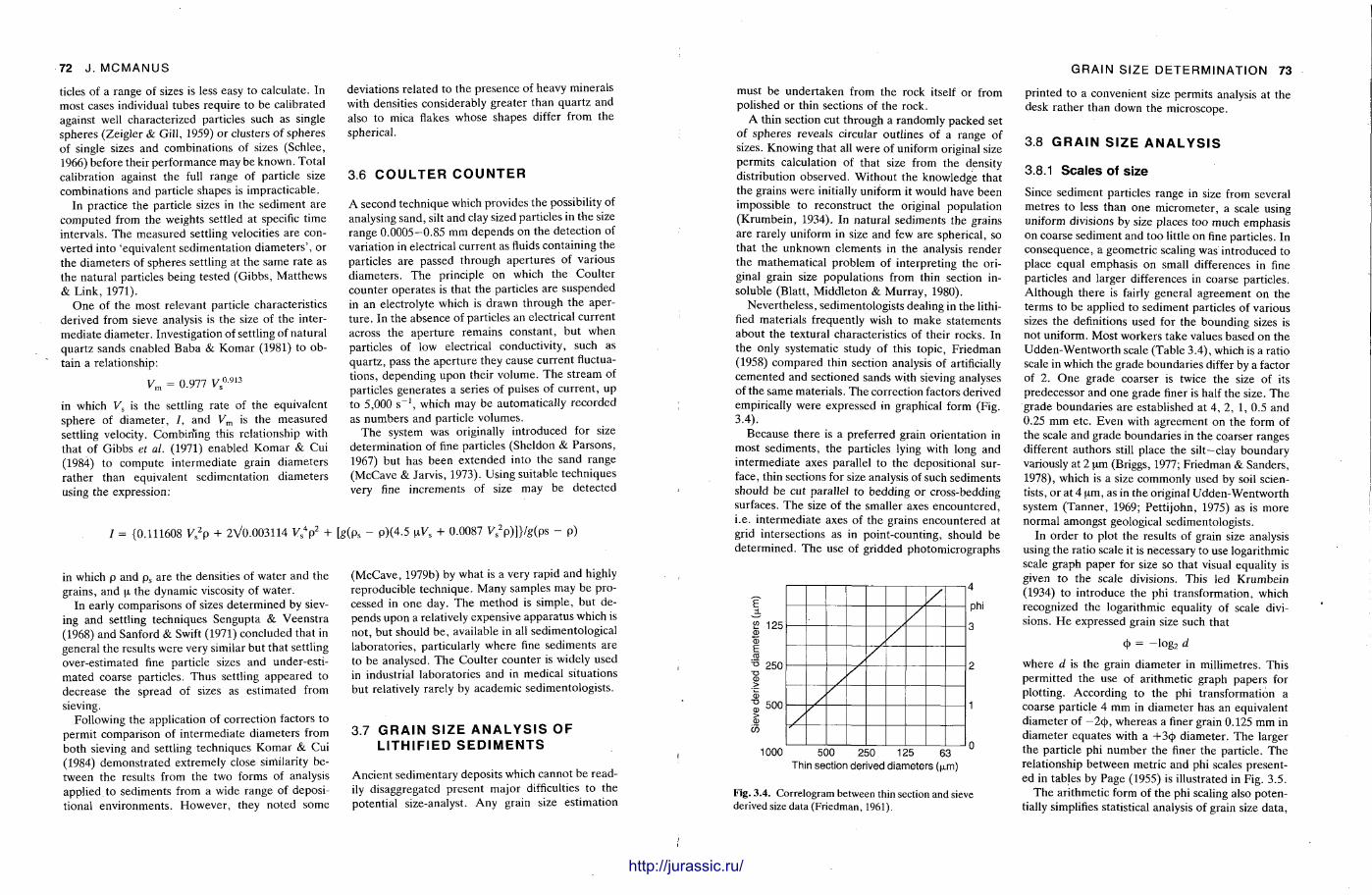
72 J . MCMANUS
t ides of a range of sizes is less easy to calculate. In most cases individual tubes require to be calibrated against well characterized particles such as single spheres (Zeigler & Gill, 1959) or clusters of spheres of single sizes and combinations of sizes (Schlee, 1966) before their performance may be known. Total calibration against the full range of particle size combinations and particle shapes is impracticable.
In practice the particle sizes in the sediment are computed from the weights settled at specific t ime intervals. T h e measured settling velocities are converted into 'equivalent sedimentat ion d iameters ' , or the diameters of spheres settling at the same rate as the natural particles being tested (Gibbs , Mat thews & Link, 1971).
One of the most relevant particle characteristics derived from sieve analysis is the size of the intermediate diameter . Investigation of settling of natural quartz sands enabled Baba & Komar (1981) to obtain a relationship:
Vm = 0.977 V™13
in which V s is the settling rate of the equivalent sphere of d iameter , / , and V m is the measured settling velocity. Combining this relationship with that of Gibbs et al. (1971) enabled Komar & Cui (1984) to compute intermediate grain diameters ra ther than equivalent sedimentat ion diameters using the expression:
/ = {0.111608 Vs
2p + 2V0.003114 V s
4p 2 +
in which p and ps are the densities of water and the grains, and p, the dynamic viscosity of water .
In early comparisons of sizes determined by sieving and settling techniques Sengupta & Veenstra (1968) and Sanford & Swift (1971) concluded that in general the results were very similar but that settling over-estimated fine particle sizes and under-estimated coarse particles. Thus settling appeared to decrease the spread of sizes as est imated from sieving.
Following the application of correction factors to permit comparison of intermediate diameters from both sieving and settling techniques Komar & Cui (1984) demonst ra ted extremely close similarity between the results from the two forms of analysis applied to sediments from a wide range of depositional environments . However , they noted some
deviations related to the presence of heavy minerals with densities considerably greater than quartz and also to mica flakes whose shapes differ from the spherical.
3.6 C O U L T E R C O U N T E R
A second technique which provides the possibility of analysing sand, silt and clay sized particles in the size range 0.0005—0.85 mm depends on the detection of variation in electrical current as fluids containing the particles are passed through aper tures of various diameters . The principle on which the Coulter counter opera tes is that the particles are suspended in an electrolyte which is drawn through the aperture . In the absence of particles an electrical current across the aper ture remains constant , but when particles of low electrical conductivity, such as quar tz , pass the aper ture they cause current fluctuations, depending upon their volume. The stream of particles generates a series of pulses of current , up to 5,000 s ~ 1 , which may be automatically recorded as numbers and particle volumes.
The system was originally introduced for size determinat ion of fine particles (Sheldon & Parsons, 1967) but has been extended into the sand range (McCave & Jarvis, 1973). Using suitable techniques very fine increments of size may be detected
fe(ps - P)(4.5 uV s + 0.0087 V s
2 p)]}/g(ps - p)
(McCave, 1979b) by what is a very rapid and highly reproducible technique. Many samples may be processed in one day. The method is simple, but depends upon a relatively expensive apparatus which is not , but should be , available in all sedimentological laboratories, particularly where fine sediments are to be analysed. The Coulter counter is widely used in industrial laboratories and in medical situations but relatively rarely by academic sedimentologists.
3.7 G R A I N S I Z E A N A L Y S I S OF L I T H I F I E D S E D I M E N T S
Ancient sedimentary deposits which cannot be readily disaggregated present major difficulties to the potential size-analyst. Any grain size estimation
GRAIN SIZE DETERMINATION 7 3
must be under taken from the rock itself or from polished or thin sections of the rock.
A thin section cut through a randomly packed set of spheres reveals circular outlines of a range of sizes. Knowing that all were of uniform original size permits calculation of that size from the density distribution observed. Without the knowledge that the grains were initially uniform it would have been impossible to reconstruct the original population (Krumbein , 1934). In natural sediments the grains are rarely uniform in size and few are spherical, so that the unknown elements in the analysis render the mathematical problem of interpreting the original grain size populat ions from thin section insoluble (Blatt , Middle ton & Murray , 1980).
Nevertheless, sedimentologists dealing in the lithified materials frequently wish to make statements about the textural characteristics of their rocks. In the only systematic study of this topic, Fr iedman (1958) compared thin section analysis of artificially cemented and sectioned sands with sieving analyses of the same materials. T h e correction factors derived empirically were expressed in graphical form (Fig. 3.4).
Because the re is a preferred grain orientation in most sediments , the particles lying with long and intermediate axes parallel to the depositional surface, thin sections for size analysis of such sediments should be cut parallel to bedding or cross-bedding surfaces. The size of the smaller axes encountered , i.e. intermediate axes of the grains encountered at grid intersections as in point-counting, should be determined. The use of gridded photomicrographs
I 1 I 1 1 1 I 1 71 1 4
E i
rs
125 B a) E CO r> 250 • 0
CD > CD
ed 500
> CD GO
1000 500 250 125 63 Thin section derived diameters (|xm)
Fig. 3 .4. Correlogram between thin section and sieve derived size data (Friedman, 1961).
printed to a convenient size permits analysis at the desk rather than down the microscope.
3.8 G R A I N S I Z E A N A L Y S I S
3.8.1 Scales of size
Since sediment particles range in size from several metres to less than one micrometer , a scale using uniform divisions by size places too much emphasis on coarse sediment and too little on fine particles. In consequence, a geometric scaling was introduced to place equal emphasis on small differences in fine particles and larger differences in coarse particles. Al though there is fairly general agreement on the terms to be applied to sediment particles of various sizes the definitions used for the bounding sizes is not uniform. Most workers take values based on the Udden-Wentwor th scale (Table 3.4), which is a ratio scale in which the grade boundaries differ by a factor of 2 . O n e grade coarser is twice the size of its predecessor and one grade finer is half the size. T h e grade boundaries are established at 4, 2, 1, 0.5 and 0.25 mm etc. Even with agreement on the form of the scale and grade boundaries in the coarser ranges different authors still place the silt—clay boundary variously at 2 urn (Briggs, 1977; Friedman & Sanders, 1978), which is a size commonly used by soil scientists, or at 4 |xra, as in the original Udden-Wentwor th system (Tanner , 1969; Pet t i john, 1975) as is more normal amongst geological sedimentologists.
In order to plot the results of grain size analysis using the ratio scale it is necessary to use logarithmic scale graph paper for size so that visual equality is given to the scale divisions. This led Krumbein (1934) to introduce the phi t ransformation, which recognized the logarithmic equality of scale divisions. H e expressed grain size such that
<h = - i o g 2 d
where d is the grain d iameter in millimetres. This permit ted the use of ari thmetic graph papers for plotting. According to the phi transformation a coarse particle 4 mm in diameter has an equivalent diameter of — 2<h, whereas a finer grain 0.125 mm in diameter equates with a +3cJ> diameter . The larger the particle phi number the finer the particle. T h e relationship between metric and phi scales presented in tables by Page (1955) is illustrated in Fig. 3.5.
The arithmetic form of the phi scaling also potentially simplifies statistical analysis of grain size data ,
l i l l l l I
http://jurassic.ru/
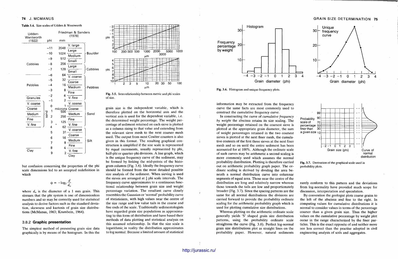
74 J . MCMANUS
Udden-Wentworth
(1922)
Friedman & Sande r s (1978)
phi mm
Cobbles
Pebbles
Granules
V. coarse
Coarse
Medium
Fine
V. fine
Clay
- 1 1
- 1 0
- 9
- 8
- 7
- 6
- 5
- 4
- 3
- 2
- 1
0
TJ 1 c CD « CO Z
3
4
5
6
7
8
9
2048
1024
512
256
128
64
32
16
8
4
2
V. large
Large
Medium
Small
Large
Small
V. coarse
Coarse
Medium
Fine
V.fine
V. coarse
Boulder
Cobbles
Pebbles
microns Coarse 500
250
125
62
31
16
8
4
2
Medium
Fine
V.fine
V. coarse
Coarse
Medium
Fine
V.fine
Clay
Sand
Silt
but confusion concerning the propert ies of the phi scale dimensions led to an accepted redefinition in which
<t> = ~log2 4-
where da is the diameter of a 1 mm grain. This stresses that the phi system is one of dimensionless numbers and so may. be correctly used for statistical analysis to derive factors such as the s tandard deviat ion, skewness and kurtosis of grain size distributions (McManus , 1963; Krumbein , 1964).
3.8.2 Graphic presentation
The simplest method of presenting grain size data graphically is by means of the histogram. In this the
- 3
phi 0
100 2001300 500 1000 2000 5000 1000 3000
phi
9 10
1 2 3 5 10 20 30 50 100
Fig. 3.5. Interrelationship between metric and phi scales of size.
grain size is the independent variable, which is therefore plotted on the horizontal axis and the vertical axis is used for the dependent variable, i.e. the determined weight percentage. The weight percentage of sediment retained on each sieve is plotted as a column rising to that value and extending from the relevant sieve mesh to the next coarser mesh used. The output from most Coulter counters is also given in this format. The resulting graphical construction is simplified if the size scale is represented by equal increments , usually represented by phi, half-phi or quarter-phi divisions. A line graph, which is the unique frequency curve of the sediment , may be formed by linking the mid-points of the histogram columns (Fig. 3.6). Ideally the frequency curve should be formed from the most detailed possible size analysis of the sediment. When sieving is used the sieves are arranged at ^ phi scale intervals. The frequency curve approximates to a cont inuous functional relationship between grain size and weight percentage variation. The resultant curve closely resembles the Gaussian or 'normal ' probability curve of statisticians, with high values near the centre of the size range and low value tails in the coarse and fine ends of the scale. Traditionally sedimentologists have regarded grain size populat ions as approximating to this form of distribution and have based their methods of data plotting and statistical analysis on this assumed relationship. In that the size scale is logarithmic in reality the distribution approximates to log normal . Because a limited amount of statistical
rfffiifffffii
GRAIN SIZE DETERMINATION 75
30 h
Frequency percentage by weight
2 0 h
1 0 h
Histogram 30
20
10
Unique frequency curve
- 4 - 3 - 2 - 1 0 1 2 3 4 Grain diameter (phi)
Fig. 3.6. Histogram and unique frequency plots.
- 4 - 3 - 2 - 1 0 1 2 3 4 Grain diameter (phi)
information may be extracted from the frequency curve the same facts are most commonly used to construct the cumulative frequency curve.
In constructing the curve of cumulative frequency by weight the abscissa retains its size scaling. The weight percentage retained on the coarsest sieve is plotted at the appropria te grain diameter , the sum of weight percentages retained in the two coarsest sieves is plotted at the next finer mesh, the cumulative contents of the first three sieves at the next finer mesh and so on until the entire sediment has been accounted for at 100%. Al though the ordinate scale of such curves may be ari thmetic a second scaling is more commonly used which assumes the normal probability distribution. Plotting is therefore carried out on ari thmetic probability graph paper . The ordinate scaling is derived by dividing the area beneath a normal distribution curve into columnar segments of equal area. Those near the centre of the distribution are long and relatively narrow whereas those towards the tails are low and proport ionately broader (Fig. 3.7). Since the spacing pat terns are the same for all normal distributions the divisions are carried forward to provide the probability ordinate scaling for the ari thmetic probability graph which is used for plotting cumulative size distributions.
Whereas plotting on the ari thmetic ordinate scale generally yields ' S ' shaped grain size distribution pat terns , using the probability ordinate scale straightens the curve (Fig. 3.8). Perfect log-normal grain size distributions plot as straight lines on the probability paper . However , natural sediments
99
Probability 9 0
scale of 70 percentage 50 finer than 30 a given size 10
1
- 2 - 1 0 1 2 3 Grain size (phi) Curve of
normal distribution
Fig. 3.7. Derivation of the graphical scale used in probability plots.
rarely conform to this pa t tern and the deviations from log-normality have provided much scope for discussion, interpretat ion and speculation.
By convention the geologist plots coarse grains to the left of the abscissa and fine to the right. In computing values for cumulative distributions it is normal to consider values in terms of the percentage coarser than a given grain size. Thus the higher values on the cumulative percentage by weight plot occur in the range characterized by the finer particles. This is the exact opposite of and neither more nor Jess correct than the practise adopted in civil engineering analysis of soils and aggregates.
Table 3.4. Size scales of Udden & Wentworth
http://jurassic.ru/
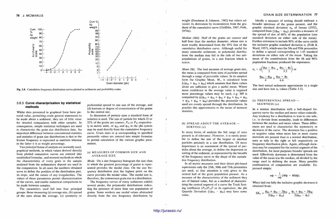
76 J . MCMANUS
Cum % b y weight
CD
E
< in
100
90
80
70
60
50
40
30
20
10
0
/
/ /
J I I I I L - 4 - 3 - 2 - 1 0 1 2 3 4
Cum % by weight
99 98 95 90 80
S 70 j § o 60 S 8 50 •- co 40
30 20 10
5 2 1
/ /
/ /
/
J I I L J I I I - 4 - 3 - 2 - 1 0 1 2 3 4
Grain diameter (phi)
Fig. 3.8. Cumulative frequency distribution curves plotted or arithmetic and probability scales.
3.8.3 Curve characterization by statistical methods
Whilst data presented in graphical form have pictorial value, permitt ing crude general s ta tements to be made about a sediment , they are of little value for detailed comparisons with other samples. In consequence, simple statistical techniques are used to characterize the grain size distribution data . A n important difference between conventional statistics and statistics of grain size distributions is that in the former frequency is expressed as numbers whereas in the latter it is as weight percentage.
Two principal forms of analysis are normally used, graphical methods , in which values derived directly from plotted cumulative curves are entered into established formulae, and moment methods in which the characteristics of every grain in the sample analysed from the sedimentary deposit are used in the computat ion. In all cases the numbers obtained serve to define the position of the distribution plot , its slope, and the nature of any irregularities. The values of these parameters permit characterization of the curves, and enable numerical comparisons to be made between samples.
The parameters used fall into four principal groups: those measuring (a)-average size, (b) spread of the sizes about the average, (c) symmetry or
preferential spread to one size of the average, and (d) kurtosis or degree of concentrat ion of the grains to the central size.
In discussion of particle sizes a s tandard form of notat ion is used. The size of particle for which 25 or 32% of the grains are coarser, F 2 s o r P32 respectively in metric units, or <j)25 and fa2 in the phi system may be read directly from the cumulative frequency curve. Grain sizes in § corresponding to specified percentile values are entered into simple formulae to permit calculation of the various graphic parameters .
(a) M E A S U R E S O F C O M M O N S I Z E A N D A V E R A G E S I Z E
Mode. O n a size frequency histogram the size class in which the greatest percentage of grains is represented provides the modal class. On the size frequency distribution plot the highest point on the curve provides the modal value. The modal size is, therefore, the commonest grain size in a distribution.
The frequency curves of many sediments exhibit several peaks , the polymodal distributions indicating the presence of more than one populat ion of grains. Some workers use modal values abstracted directly from the size frequency distribution by
GRAIN SIZE DETERMINATION 77
weight (Friedman & Johnson, 1982) but others advocate its derivation by recalculation from the gradient of the cumulative curve (Griffiths, 1967; Folk, 1974b).
Median (Md). Half of the grains are coarser and half finer than the median diameter , whose size is most readily determined from the 5 0 % line of the cumulative distribution curve. Although useful for many unimodal sediments , in polymodal distributions the median may fall in the tails of two sub-populat ions of grains, in a size fraction which is scarce.
Mean (M). The best measure of average grain size, the mean is computed from sizes of particles spread through a range of percentile values. In its simplest form the Graphic Mean , M , , is calculated from
( tp 1 6 + c|>5o + <j>84) which assumes that three values alone are sufficient to give a useful mean. Where more confidence in the average value is required more percentage values may be used, e.g. M9 is computed by £((b 1 ( , + 4>2„ + 4>3(, + <t>40 + (b 5 0 + <l>60 + <|>7o + (j>8o + 4>9o) provided the percentile values used are evenly spread through the distribution. In practise this approximates to the mean of moment statistics.
(b) S P R E A D A B O U T T H E A V E R A G E — S O R T I N G (a)
In many forms of analysis the full range of sizes present is of relevance. However , it is rarely possible to define the size of the largest or smallest particles precisely in a size distribution. Of more importance is an assessment of the spread of particles about the average, to define the dispersion or sorting of the sediment, as represented by the breadth of the frequency curve or the shape of the cumulative frequency distribution.
In all metric measures and their direct phi-based equivalents only the 25th, 50th and 75th percentiles are used, so that at tention is only given to the central half of the grain populat ion present . As a measure of the characteristics of the sediment they are of limited value, but as a method of characterizing the central segment of a curve the Trask Sorting coefficient ( / W ^ s ) - o r i t s equivalent, the phi Quart i le Deviation y((j>75 — (fes) may have some value.
Ideally a measure of sorting should embrace a broader spectrum of the grains present , and the graphic s tandard deviation o^ of Inman (1952), computed from ^(<t>84 - (j>16), provides a measure of the spread of size of 6 8 % of the population (one s tandard deviation on ei ther side of the mean) . Fur ther extension to include 90% of the curve yields the inclusive graphic s tandard deviation Oi (Folk & Ward , 1957), which uses the 5th and 95th percentiles to define a spread corresponding to 1.65 standard deviations on either side of the mean. Taking the mean of the contributions from the 68 and 9 0 % populat ion fractions produced the expression:
„ _ 1 /<l>84 ~ <|>16 , 4>95 ~ <t>s\ n r
01 ~ A 2 + 3.3 Jor
<t>84 ~ <t>16 , <j>95 ~ <t>5 4 6.6 '
The best sorted sediments approximate to, a single size and have low O) values (Table 3.5).
(c) P R E F E R E N T I A L S P R E A D — S K E W N E S S (a)
In a normal distribution with a bell-shaped frequency curve the median and mean values coincide. Any tendency for a distribution to lean to one side, i .e. to deviate from normali ty, leads to differences between the median and mean values. These differences are used to characterize the asymmetry or skewness of the curve. The skewness has a positive or negative value when more fine or more coarse materials are present than in a normal distribution, seen as tails to the right or left respectively on frequency distribution plots. Again , al though skewness may be computed for the central segment of the distribution, for most purposes broader spreads are used. Effectively skewness is determined from the value of the mean less the median, all divided by the range used in defining the mean. Many possible combinations of computat ion are available. Expressed simply:
a<j> = ^ ( M < b - Md$).
When laid out fully the inclusive graphic skewness is obtained from:
S K = 4>16 + <t>S4 ~ 2c()so 4>5 + (j)95 - 2(j>50 1 2(<j)g4 - <b 1 6) 2((j>9 5 - cb 5)
• http://jurassic.ru/
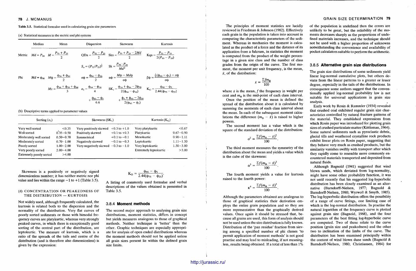
78 J . MCMANUS
Median Mean Dispersion Skewness Kurtosis
Metric Md = P,„ M • P75 + ^25 2
Phi Md = <j)50 Azcj) =
PlS P 25 c . QDa = Ska ;
So = (Pis/Pis)* Sk
<l>84 - <t>16
P 7 s + P „ - 2Md Kqa P75 ~ P25
2(Pc)o — P10)
Otj)
Mz = a, =
995 V5
6.6
a<t> -
SK,
M d 2
M(() - Md$ o<()
<t>16 + <1>84 — 2<t>5l
ocj)
+
2(<t>«4 -
<t>5 + <t>9:
>1&)
- 2<t»50
2.44(<t>75-ij>25)
2(4>95 - <t>s)
(b) Descriptive terms applied to parameter values
Sorting (o t ) Skewness (SKj) Kurtosis (K G )
Very well sorted <0.35 Very positively skewed +0.3 to +1.0 Very platykurtic <0.67 Well sorted 035-0 .50 Positively skewed +0.1 to +0.3 Platykurtic 0.67-0.90 Moderately well sorted 0.50-0.70 Symmetrical +0.1 to -0 .1 Mesokurtic 0.90-1.11 Moderately sorted 0.70-1.00 Negatively skewed - 0 . 1 t o - 0 . 3 Leptokurtic 1.11-1.50 Poorly sorted 1.00-2.00 Very negatively skewed - 0 . 3 t o - 1 . 0 Very leptokurtic 1.50-3.00 Very poorly sorted 2.00-4.00 Extremely leptokurtic >3.00 Extremely poorly sorted >4.00
Skewness is a positively or negatively signed dimensionless number ; it has nei ther metr ic nor phi value and lies within the range —1 to + 1 (Table 3.5).
(d) C O N C E N T R A T I O N O R P E A K E D N E S S O F T H E D I S T R I B U T I O N — K U R T O S I S
Not widely used, although frequently calculated, the kurtosis is related both to the dispersion and the normality of the distribution. Very flat curves of poorly sorted sediments or those with bimodal frequency curves are platykurtic, whereas very strongly peaked curves, in which there is exceptionally good sorting of the central par t of the distribution, are leptokurt ic . The measure of kurtosis, which is a ratio of the spreads of the tails and centre of the distribution (and is therefore also dimensionless) is given by the expression:
4>95 ~ 4>5 2.44(<J,75 " 4>25)'
A listing of commonly used formulae and verbal descriptions of the values obtained is presented in Table 3.5.
3.8.4 Moment methods
The second major approach to analysing grain size distributions, momen t statistics, differs in concept but yields measures analogous to those of graphical methods . Nei ther technique is 'bet ter ' than the other . Graphic techniques are especially appropria te for analysis of open ended distributions whereas the moment methods should not be applied unless all grain sizes present lie within the defined grain size limits.
GRAIN SIZE DETERMINATION 79
The principles of momen t statistics are lucidly reviewed in Fr iedman & Johnson (1982). Effectively each grain in the populat ion is taken into account in computing the characteristic parameters of the sediment . Whereas in mechanics the moment is calculated as the product of a force and the distance of its application from a fulcrum, in statistics the moment is computed from the product of the weight percentage in a given size class and the number of class grades from the origin of the curve. The first moment , the moment per unit frequency, is the mean , x, of the distribution:
x = 100
where x is the mean, / the frequency in weight per cent and is the mid-point of each class interval.
Once the position of the mean is defined the spread of the distribution about it is calculated by summing the moments of each class interval about the mean . In each of the subsequent moment calculations the difference (m^ - x) is raised to higher powers .
The second moment has a value which is the square of the standard deviation of the distribution:
, Lf(m^ - xf ^ = — T o o — •
The third momen t measures the symmetry of the distribution about the mean and yields a value which is the cube of the skewness:
, Lf(m^ - xf 100
T h e fourth momen t yields a value for kurtosis raised to the fourth power:
4 _ E/(m,|, - xf 100
Al though the parameters obtained are analogous to those of graphical statistics their derivation employs the entire grain populat ion and so they are more representat ive than the graphically derived values. Once again it should be stressed that , because all grains are used, this form of analysis should not be used unless the size distribution is fully known. Distr ibution of the 'pan residue ' fraction from sieving among a specified number of phi classes ' to permit application of moment methods ' is not good practise and may lead to misleading, if not meaning-
. less, results being obtained. If a total of less than 1%
of the populat ion is undefined then the errors are unlikely to be great , but the reliability of the moments decreases sharply as the proport ions of undefined materials increases, and the technique should not be used with a higher propor t ion of unknowns notwithstanding the convenience and availability of pocket calculators suitable to perform the ari thmetic.
3.8.5 Alternative grain size distr ibut ions
The grain size distributions of some sediments yield linear log-normal cumulative plots , but others deviate from the linear pa t te rns to a greater or lesser degree , especially in the tails of the distributions. In consequence some authors suggest that the conventionally applied log-normal probability law is not suitable for universal applications in grain size analysis.
Early work by Rosin & Rammler (1934) revealed that -crushed coal exhibited regular grain size characteristics controlled by natural fracture pat terns of the material . They established expressions from which Rosin paper was introduced for plotting grain sizes of crushed particulate mat te r (Kit t leman, 1964). Some natural sediments such as pyroclastic debris , glacial tills and weathered crystalline rock products exhibit l inear plots on Rosin paper , suggesting that they behave very much as crushed products , but the similarity vanishes swiftly with transport after which they rapidly come to resemble more commonly encountered materials t ranspor ted and deposited from natural fluids.
Al though Bagnold (1941) suggested that wind blown sands , which deviated from log-normality, might have some other probability function, it was not until recently that his suggested log-hyperbolic distribution has been closely examined as an alternative (Barndorff-Nielsen, 1977; Bagnold & Barndorff-Nielsen, 1980; Wyrwoll & Smyth, 1985). The log-hyperbolic distribution offers the possibility of a range of curve fittings, one limiting case of which is the log-normal distribution. In practise the natural logarithm of the frequency curve is plotted against grain size (Bagnold, 1968), and the four parameters of the best fitting log-hyperbolic curve are computed . Two of these relate to the curve position (grain size and peakedness) and the other two to inclination of the limbs of the curve. The distribution has been examined principally within the context of wind blown dune sands (Bagnold & Barndorff-Nielsen, 1980; Christiansen, 1984) for
Table 3 . 5 . Statistical formulae used in calculating grain size parameters
(a) Statistical measures in the metric and phi systems
http://jurassic.ru/
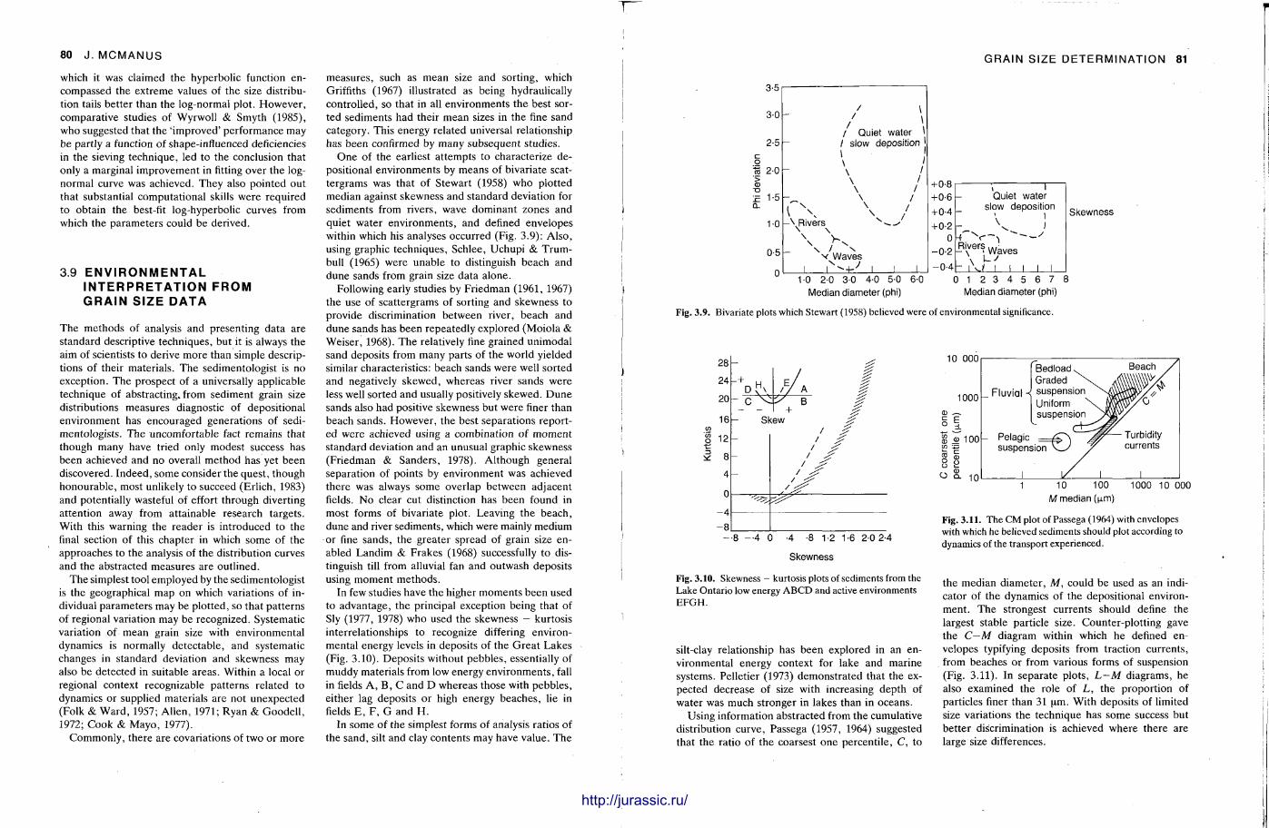
80 J . MCMANUS
3.9 E N V I R O N M E N T A L I N T E R P R E T A T I O N F R O M G R A I N S I Z E D A T A
The methods of analysis and presenting data are standard descriptive techniques, but it is always the aim of scientists to derive more than simple descriptions of their materials. The sedimentologist is no exception. The prospect of a universally applicable technique of abstracting, from sediment grain size distributions measures diagnostic of depositional environment has encouraged generat ions of sedimentologists. The uncomfortable fact remains that though many have tried only modest success has been achieved and no overall method has yet been discovered. Indeed, some consider the quest , though honourable , most unlikely to succeed (Erlich, 1983) and potentially wasteful of effort through diverting attention away from attainable research targets. With this warning the reader is introduced to the final section of this chapter in which some of the approaches to the analysis of the distribution curves and the abstracted measures are outlined.
The simplest tool employed by the sedimentologist is the geographical map on which variations of individual parameters may be plotted, so that pat terns of regional variation may be recognized. Systematic variation of mean grain size with environmental dynamics is normally detectable , and systematic changes in standard deviation and skewness may also be detected in suitable areas . Within a local or regional context recognizable pat terns related to dynamics or supplied materials are not unexpected (Folk & Ward , 1957; Allen, 1971; Ryan & Goodel l , 1972; Cook & Mayo, 1977).
Commonly , there are covariations of two or more
measures , such as mean size and sorting, which Griffiths (1967) illustrated as being hydraulically controlled, so that in all environments the best sorted sediments had their mean sizes in the fine sand category. This energy related universal relationship has been confirmed by many subsequent studies.
O n e of the earliest a t tempts to characterize depositional environments by means of bivariate scat-tergrams was that of Stewart (1958) who plotted median against skewness and standard deviation for sediments from rivers, wave dominant zones and quiet water environments , and defined envelopes within which his analyses occurred (Fig. 3.9): Also , using graphic techniques, Schlee, Uchupi & Trumbull (1965) were unable to distinguish beach and dune sands from grain size data a lone.
Following early studies by Fr iedman (1961, 1967) the use of scattergrams of sorting and skewness to provide discrimination between river, beach and dune sands has been repeatedly explored (Moiola & Weiser , 1968). The relatively fine grained unimbdal sand deposits from many parts of the world yielded similar characteristics: beach sands were well sorted and negatively skewed, whereas river sands were less well sorted and usually positively skewed. D u n e sands also had positive skewness but were finer than beach sands. However , the best separat ions reported were achieved using a combination of moment standard deviation and an unusual graphic skewness (Friedman & Sanders , 1978). Al though general separation of points by environment was achieved there was always some overlap between adjacent fields. No clear cut distinction has been found in most forms of bivariate plot. Leaving the beach, dune and river sediments, which were mainly medium or fine sands, the greater spread of grain size enabled Landim & Frakes (1968) successfully to distinguish till from alluvial fan and outwash deposits using moment methods .
In few studies have the higher moments been used to advantage, the principal exception being that of Sly (1977, 1978) who used the skewness — kurtosis interrelationships to recognize differing environmental energy levels in deposits of the Grea t Lakes (Fig. 3.10). Deposits without pebbles , essentially of muddy materials from low energy envi ronments , fall in fields A , B , C and D whereas those with pebbles , either lag deposits or high energy beaches , lie in fields E , F , G and H .
In some of the simplest forms of analysis ratios of the sand, silt and clay contents may have value. The
illllllllllllllilllll
GRAIN SIZE DETERMINATION 81
3-5
3-0
2-5 c o to 2-0 > CD
•o Z 1-5 Q-
1-0
0-5
0
/ \ / Quiet water i / slow deposition ] I \ \
- \Rivers
\ I ^ v Waves \ j
+0-8 +0-6 +0-4 + 0-2
0
Quiet water slow deposition
I I
4 ^<—s - - ' /
- 0 - 2 - R i
N
v e r S l ' Waves
0-4h iVy J _ J I L 1-0 2-0 3-0 4-0 5-0
Median diameter (phi) 6-0
Skewness
0 1 2 3 4 5 6 7 8 Median diameter (phi)
Fig. 3 . 9 . Bivariate plots which Stewart (1958) believed were of environmental significance.
- 4 !
-81 I - • 8 —4 0 -4 -8 1-2 1-6 2 0 2-4
Skewness
Fig. 3.10. Skewness - kurtosis plots of sediments from the Lake Ontario low energy ABCD and active environments EFGH.
silt-clay relationship has been explored in an environmental energy context for lake and marine systems. Pelletier (1973) demonst ra ted that the expected decrease of size with increasing depth of water was much stronger in lakes than in oceans.
Using information abstracted from the cumulative distribution curve, Passega (1957, 1964) suggested that the ratio of the coarsest one percenti le, C, to
10 000
1000 _ Fluvial -
Bedload. Graded \ . suspension \ Uniform \ suspension J
Beach /
Pelagic — / C \ /W suspension VL_y /
i y i
^— Turbidity currents
I 1 10 100 1000 10 000
M median (u,m)
Fig. 3.11. The CM plot of Passega (1964) with envelopes with which he believed sediments should plot according to dynamics of the transport experienced.
the median diameter , M, could be used as an indicator of the dynamics of the depositional environment . The strongest currents should define the largest stable particle size. Counter-plott ing gave the C—M diagram within which he defined envelopes typifying deposits from traction currents , from beaches or from various forms of suspension (Fig. 3.11). In separate plots, L—M diagrams, he also examined the role of L , the proport ion of particles finer than 31 um. With deposits of limited size variations the technique has some success but bet ter discrimination is achieved where there are large size differences.
which it was claimed the hyperbolic function encompassed the extreme values of the size distribution tails bet ter than the log-normal plot. However , comparat ive studies of Wyrwoll & Smyth (1985), who suggested that the ' improved ' performance may be partly a function of shape-influenced deficiencies in the sieving technique, led to the conclusion that only a marginal improvement in fitting over the log-normal curve was achieved. They also pointed out that substantial computat ional skills were required to obtain the best-fit log-hyperbolic curves from which the parameters could be derived.
http://jurassic.ru/
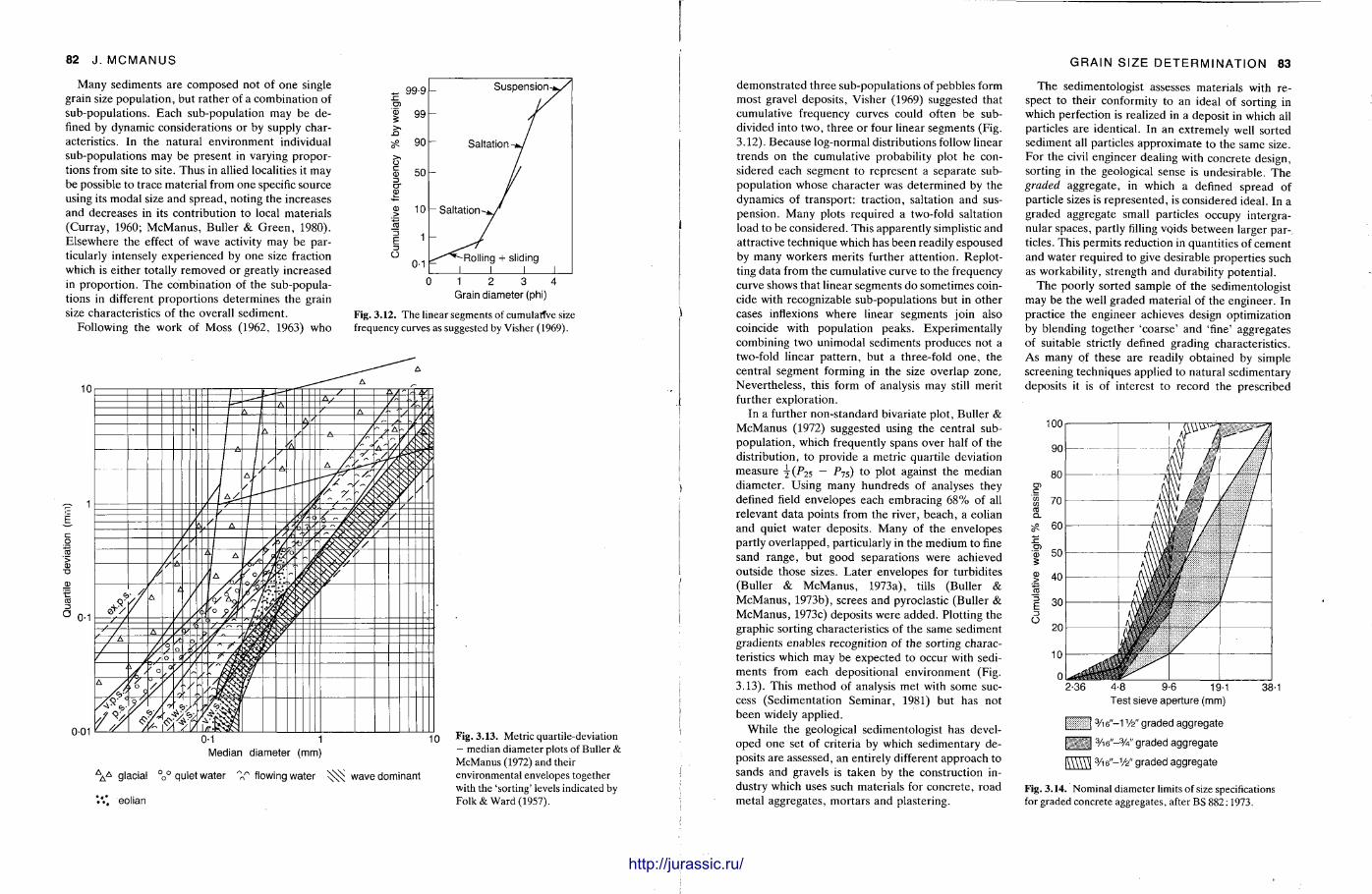
82 J. MCMANUS
Many sediments are composed not of one single grain size populat ion, but ra ther of a combinat ion of sub-populations. Each sub-population may be defined by dynamic considerations or by supply characteristics. In the natural environment individual sub-populations may be present in varying proportions from site to site. Thus in allied localities it may be possible to trace material from one specific source using its modal size and spread, noting the increases and decreases in its contribution to local materials (Curray, 1960; McManus , Buller & Green , 1980). Elsewhere the effect of wave activity may be particularly intensely experienced by one size fraction which is either totally removed or greatly increased in proport ion. The combination of the sub-populations in different proport ions determines the grain size characteristics of the overall sediment.
Following the work of Moss (1962, 1963) who
„ 99-9 h CD
>>
D -
E o
99
90 h 50 h 10
0-1
Suspension-,
Saltation-
• Saltation-
-Rolling + sliding J I I
0 1 2 3 4 Grain diameter (phi)
Fig. 3.12. The linear segments of cumulative size frequency curves as suggested by Visher (1969).
0-1 1 Median diameter (mm)
^ A glacial 0
0 ° quiet water flowing water wave dominant
'.' eolian
Fig. 3.13. Metric quartile-deviation - median diameter plots of Buller & McManus (1972) and their environmental envelopes together with the 'sorting' levels indicated by Folk & Ward (1957).
r
demonst ra ted three sub-populations of pebbles form most gravel deposits , Visher (1969) suggested that cumulative frequency curves could often be subdivided into two, three or four linear segments (Fig. 3.12). Because log-normal distributions follow linear trends on the cumulative probability plot he considered each segment to represent a separate sub-population whose character was determined by the dynamics of t ransport : traction, saltation and suspension. Many plots required a two-fold saltation
' load to be considered. This apparently simplistic and attractive technique which has been readily espoused by many workers merits further at tent ion. Replot-ting data from the cumulative curve to the frequency curve shows that linear segments do sometimes coincide with recognizable sub-populations but in other
) cases inflexions where linear segments join also coincide with populat ion peaks . Experimentally combining two unimodal sediments produces not a two-fold linear pa t te rn , but a three-fold one , the central segment forming in the size overlap zone. Nevertheless, this form of analysis may still merit further exploration.
In a further non-standard bivariate plot, Buller & McManus (1972) suggested using the central sub-populat ion, which frequently spans over half of the distribution, to provide a metric quartile deviation measure y ( P 2 5 — P75) to plot against the median
) diameter . Using many hundreds of analyses they defined field envelopes each embracing 6 8 % of all relevant data points from the river, beach, a eolian and quiet water deposits . Many of the envelopes partly over lapped, particularly in the medium to fine sand range , but good separations were achieved outside those sizes. La te r envelopes for turbidites
' (Buller & McManus , 1973a), tills (Buller & McManus , 1973b), screes and pyroclastic (Buller & McManus , 1973c) deposits were added. Plotting the graphic sorting characteristics of the same sediment gradients enables recognition of the sorting characteristics which may be expected to occur with sediments from each depositional environment (Fig.
j 3.13). This method of analysis met with some success (Sedimentat ion Seminar , 1981) but has not
I been widely applied. i While the geological sedimentologist has devel
oped one set of criteria by which sedimentary deposits are assessed, an entirely different approach to
! sands and gravels is taken by the construction industry which uses such materials for concrete , road metal aggregates, mortars and plastering.
GRAIN SIZE DETERMINATION 8 3
The sedimentologist assesses materials with respect to their conformity to an ideal of sorting in which perfection is realized in a deposit in which all particles are identical. In an extremely well sorted sediment all particles approximate to the same size. For the civil engineer dealing with concrete design, sorting in the geological sense is undesirable. The graded aggregate, in which a defined spread of particle sizes is represented , is considered ideal. In a graded aggregate small particles occupy intergra-nular spaces, partly filling voids between larger particles. This permits reduction in quanti t ies of cement and water required to give desirable propert ies such as workabili ty, strength and durability potential .
T h e poorly sorted sample of the sedimentologist may be the well graded material of the engineer. In practice the engineer achieves design optimization by blending together 'coarse ' and 'fine' aggregates of suitable strictly defined grading characteristics. As many of these are readily obtained by simple screening techniques applied to natural sedimentary deposits it is of interest to record the prescribed
2-36 4-8 9-6 19-1 38-1 Test sieve aperture (mm)
[ j 3/i6"-1 V2" graded aggregate
.] 3/i6"- 3A" graded aggregate
|\\\\\^ 3/i6"-1/2" graded aggregate
Fig. 3.14. Nominal diameter limits of size specifications for graded concrete aggregates, after BS 882:1973.
i l l http://jurassic.ru/
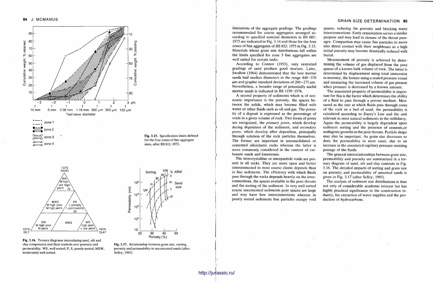
84 J . MCMANUS
1 0 0 %
C L A Y 20 30 40 50 Porosity (%)
Fig. 3.16. Ternary diagrams interrelating sand, silt and clay components and their controls over porosity and Fig. 3.17. Relationship between grain size, sorting, permeability. WS, well sorted; P, S, poorly sorted; MSW, porosity and permeability in uncemented sands (after moderately well sorted. Selley, 1985).
GRAIN SIZE DETERMINATION 85
limitations of the aggregate gradings. The gradings recommended for coarse aggregates arranged according to specified nominal diameters in BS 882: 1973 are indicated in Fig. 3.14 and those for the four zones of fine aggregates of BS 812: 1975 in Fig. 3.15. Materials whose grain size distributions fall within the limits specified for zone 3 fine aggregates are well suited for certain tasks.
According to Connor (1953), only restricted gradings of sand produce good mortars . Later , Swallow (1964) demonst ra ted that the best mortar sands had median diameters in the range 440—570 urn and graphic standard deviations of 2 0 0 - 2 7 5 pm. Nevertheless, a broader range of potentially useful mor tar sands is indicated in BS 1199:1976.
A second proper ty of sediments which is of eco-' nomic importance is the porosity, the spaces be
tween the solids, which may become filled with water or o ther fluids such as oil and gas. The porosity of a deposit is expressed as the percentage of voids in a given volume of rock. Two forms of pores are recognized, the primary pores, which develop
I during deposition of the sediment , and secondary pores, which develop after deposit ion, principally through solution of the rock particles themselves. The former are important in unconsolidated or cemented siliciclastic rocks whereas the latter is more commonly considered in the context of car-
) bonate sands and l imestones. The intercrystalline or interparticle voids are pre
sent in all rocks. They are more open and bet ter interconnected in most coarse clastic deposits than in fine sediments . The efficiency with which fluids pass through the rocks depends heavily on the inter-
t connections, the spaces available in the pore throats and the sorting of the sediment . In very well sorted coarse uncemented sediments pore spaces are large and may have free interconnections whereas in poorly sorted sediments fine particles occupy void
spaces, reducing the porosity and blocking many interconnections. Early cementat ion serves a similar purpose and may lead to closure of the throat passages. Compact ion may cause fine particles to move into direct contact with their neighbours so a high initial porosity may become drastically reduced with burial.
Measurement of porosity is achieved by determining the volume of gas displaced from the pore spaces of a known bulk volume of rock. T h e latter is determined by displacement using total immersion in mercury, the former using a sealed pressure vessel and measuring the increased volume of gas present when pressure is decreased by a known amount .
The associated property of permeability is important for this is the factor which determines the ability of a fluid to pass through a porous medium. Measured as the ra te at which fluids pass through cores of the rock or a bed of sand, the permeability is calculated according to Darcy 's Law and the unit relevant in most natural sediments in the millidarcy. Again the permeabili ty is largely dependent upon sediment sorting and the presence of cements ,or authigenic growths in the pore throats . Particle shape may also be important . As grain size decreases so does t he permeability in most cases, due t o an increase in the associated capillary pressure resisting passage of the fluids.
T h e general interrelationships between grain size, permeabil i ty and porosity are summarized in a ternary diagram of sand, silt and clay contents in Fig. 3.16. The detailed impacts of sorting and grain size on porosity and permeabili ty of unsorted sands is given in Fig. 3.17 (after Selley, 1985).
The analysis of sediment size distributions is thus not only of considerable academic interest but has highly practical significance to the construction industry, for extraction of water supplies and the production of hydrocarbons.
i http://jurassic.ru/
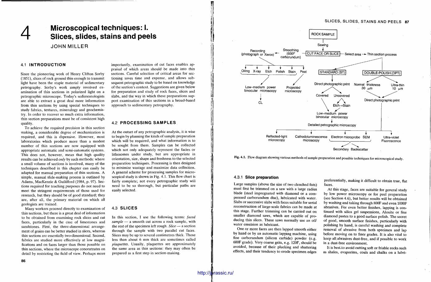
4 Microscopical techniques: I. Slices, slides, stains and peels JOHN MILLER
4.1 I N T R O D U C T I O N
Since the pioneering work of Henry Clifton Sorby (1851), slices of rock ground thin enough to transmit light have been the staple material of sedimentary petrography. Sorby's work simply involved examination of thin sections in polarized light on a petrographic microscope. Today 's sedimentologists are able to extract a great deal more information from thin sections by using special techniques to study fabrics, textures , mineralogy and geochemistry. In order to recover so much extra information, thin section preparat ions must be of consistent high quality.
To achieve the required precision in thin section making, a considerable degree of mechanization is required, and this is expensive. However , most laboratories which produce more than a modest number of thin sections are now equipped with appropr ia te automat ic and semi-automatic systems. This does not , however, mean that high quality results can be achieved only by such methods : where a small volume of sections is involved, many of the techniques described in this chapter can easily be adapted for manual preparat ion of thin sections. A simple, manual slide-making process is outl ined by A d a m s , MacKenzie & Guildford (1984, p . 97). Sections required for teaching purposes do not need to meet the stringent requirements of those used for research, but they should be of good s tandard; they a re , after all, the primary material on which all geologists are trained.
Many workers proceed directly to examination of thin sections, but there is a great deal of information to be obtained from examining rock slices and cut faces, particularly in the case of limestones and sandstones. First, the three-dimensional arrangement of grains can be better studied in slices, whereas thin sections are essentially two-dimensional. Second, fabrics are studied more effectively at low magnifications and on faces larger than those possible on thin sections, where the microscope concentrates on detail by restricting the field of view. Perhaps more
86
important ly, examination of cut faces enables appraisal of which areas should be made into thin sections. Careful selection of critical a reas for sectioning saves t ime and expense, and allows subsequent petrographic study to be based on knowledge of the section's context . Suggestions are given below for preparat ion and study of rock faces, slices and slabs, and the way in which these preparat ions support examination of thin sections in a broad-based approach to sedimentary petrography.
4.2 P R O C E S S I N G S A M P L E S
At the outset of any petrographic analysis, it is wise to begin by planning the kinds of sample preparat ion which will be required, and what information is to be sought from them. Samples can be collected which not only adequately represent the facies or lithosomes under study, but are appropr ia te in or ientat ion, size, shape and freshness to the selected preparat ion techniques. Processing is then designed to minimize wastage and maximize data collection. A general scheme for processing samples for microscopical study is shown in Fig. 4 . 1 . This flow chart is fairly complete ; not every petrographic study will need to be so thorough, but particular paths are easily selected.
4.3 S L I C E S
In this section, I use the following terms: faced sample — a smooth cut across a rock sample, with the rest of the specimen left rough. Slice — a section through the sample with two parallel cut faces. Slices may be up to several centimetres thick. Those less than about 6 mm thick are sometimes called plaquettes. Usually, plaquet tes are approximately the same area as thin sections: they may often be prepared as a first step in section-making.
SLICES, SLIDES, STAINS AND PEELS 8 7
ROCK SAMPLE
Recording Smoothing (photograph or Xerox) ( 6 0 0 F
carborundum)
* J \ J } Oiling X-ray Etch Polish Stain Peel
-J
Sawing I
CUT FACE OR SLICE |— Select area Thin section process
Low-medium power Projected binocular microscopy microscopy
J CL
Direct photographic print Normal thickness Ultra-thin 30 vm 10 ixm
Covered Uncovered
/ \ Etch^Stain
Low-medium power binocular microscopy
\ Detailed petrographic microscopy
Direct photographic print
J \ j r Reflected-light Cathodoluminescence Electron microprobe SEM
microscopy microscopy ^ > Ultra-violet
Fluorescence
Secondary Backscatter
Fig. 4.1. Flow diagram showing various methods of sample preparation and possible techniques for microscopical study.
4.3.1 Slice preparation
Large samples (above the size of two clenched fists) must first b e t r immed on a saw with a large radius blade (steel impregnated with diamond or a compressed carborundum disc), lubricated with water . Slabs or successive slabs with faces suitable for serial reconstruction of large-scale fabrics can be made at this stage. Fur ther trimming can be carried out on smaller d iamond saws, which are capable of producing thin slices. These saws normally use an oil/ water emulsion as lubricant.
O n e or more faces a re then lapped smooth either by hand or by an automatic lapping machine, using fine carborundum (silicon carbide) powder (e .g. 600F grade) . Very coarse grits, e.g. 120F, should be avoided, because of their plucking and shattering effects, and their tendency to erode specimen edges
preferentially, making it difficult t o obtain t rue , flat faces.
At this stage, faces are suitable for general study by low power microscopy or for peel preparat ion (see Section 4.6), but bet ter results will be obtained by washing and taking through 800F and even 1000F abrasives. For even better finishes, lapping is cont inued with silica gel suspensions, Aloxite or fine diamond pastes to a good surface polish. The secret of good, smooth surface finishes, particularly with polishing by hand , is careful washing and complete removal of abrasive from both specimen and lap before moving on to finer grades. It is also vital to keep alLabrasives dust-free, and if possible to work in a dust-free environment .
It is best-to avoid cutting soft or friable rocks such as shales, evapori tes , coals and chalks on a lubri-
I 111 http://jurassic.ru/
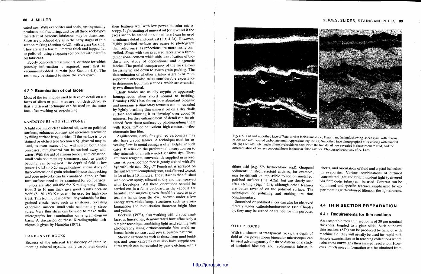
88 J . MILLER
cated saw. With evapori tes and coals, cutt ing usually produces bad fracturing, and for all th ree rock-types the effect of aqueous lubricants may be disastrous. Slices are produced dry as in the early stages of thin section making (Section 4.4.2) , with a glass backing. They are left a few millimetres thick and lapped flat or polished, using a lapping compound with paraffin oil lubricant.
Poorly consolidated sediments , or those for which porosity information is required, must first be vacuum-imbedded in resin (see Section 4.5). T h e resin may be stained to show the void space.
4.3.2 Examination of cut faces
Most of the techniques used to develop detail on cut faces of slices or plaquet tes are non-destructive, so that a different technique can be used on the same face after washing or re-polishing.
S A N D S T O N E S A N D S I L T S T O N E S
A light coating of clear mineral oil, even on polished surfaces, enhances contrast and increases resolution by filling surface irregularities. If the surface is to be stained or etched (see Section 4.5) , glycerol may be used, as even traces of oil will inhibit both these processes, but glycerol can be washed away with water . With the aid of a zoom binocular microscope, small-scale sedimentary structures, such as graded bedding, can be viewed. The depth of field at low power ( x l . 5 to X20 magnification) allows study of three-dimensional grain relationships so that packing and pore networks can be visualized, al though fracture surfaces need to be examined for comparison.
Slices are also suitable for X-radiography. Slices from 3 to 10 m m thick give good results because 'soft' (5—50 kV) X-rays can be used for high contrast. This technique is particularly valuable for finegrained clastic rocks such as siltstones, revealing otherwise unseen small-scale sedimentary structures . Very thin slices can be used to m a k e radio-micrographs for examination on a grain-to-grain basis. A discussion of these X-radiographic techniques is given by Hambl in (1971).
C A R B O N A T E R O C K S
Because of the inherent translucency of their cementing mineral crystals, many carbonates display
their features well with low power biocular microscopy. Light coating of mineral oil (or glycerol if the faces are to be etched or stained later) can be used to enhance detail and contrast (Fig. 4.2a). However , highly polished surfaces are easier to photograph than oiled ones , as reflections are more easily controlled. Slices with two prepared faces give a three-dimensional context which aids identification of bio-clasts and study of depositional and diagenetic fabrics. The partial t ransparency of the rock allows focussing up and down to assess grain packing. The determinat ion of whether a fabric is grain- or mud-supported otherwise takes considerable experience to determine from thin sections, which are essentially two-dimensional.
Chalk fabrics are usually cryptic or apparently homogeneous when sliced normal to bedding. Bromley (1981) has shown how abundant biogenic and inorganic sedimentary textures can be revealed by lightly brushing thin mineral oil on a dry chalk surface and allowing it to 'develop ' over about 30 minutes. Fur ther enhancement of detail can be obtained from these surfaces by photographing them with Kodalith® o r equivalent high-contrast o r tho-chromatic line film.
Argil laceous, dark , fine-grained carbonates may also have cryptic fabrics. A technique used for revealing flaws in metal casings is often helpful in such cases. It relies on the preferential absorpt ion on to clay minerals of an ultra-violet sensitive dye. T h e r e are three reagents , conveniently supplied in aerosol cans. A pre-smoothed face is gently etched with 5 % hydrochloric acid. Zyglo® Penet ran t is sprayed on the surface until completely wet , and allowed to soak in for at least 10 minutes . The surface is then flushed with Solvent spray, allowed to dry and then sprayed with Developer . All these operat ions should be carried out in a fume cupboard as the vapours are harmful, and surgical gloves should be used to protect the hands from the dye. Viewed under a low energy ultra-violet lamp, structures such as cross-lamination and bioturbation fluoresce bright blue and yellow.
Bockelie (1973), also working with cryptic argillaceous l imestones, demonstra ted how effectively a simpler technique combining light acid etching with photography using or thochromat ic film could enhance fabric contrast and reveal burrow pat terns .
Micritic carbonates such as those from mud buildups and some calcretes may also have cryptic textures which can be revealed by gentle etching with a
SLICES, SLIDES, STAINS AND PEELS 89
Fig. 4.2. Cut and smoothed face of Waulsortian facies limestone, Dinantian, Ireland, showing 'sheet spars' with fibrous ca cite and i n t e r f e r e d carbonate mud. Approximately x2. (a) Smoothed face photographed after coating with mineral oil (b) Face after etching in dilute hydrochloric acid. Note the fine detail now revealed in the carbonate mud and the differentiation of coarser geopetal floors in the spar-filled cavities. Photographs courtesy of A Lees
dilute acid (e.g. 5 % hydrochloric acid). Geopeta l sediments in s t romatactoid cavities, for example , may be difficult or impossible to see on unetched, polished surfaces (Fig. 4.2a) , but are clearly seen after etching (Fig. 4.2b), al though other features are bet ter revealed on the polished surface. T h e techniques of polishing and etching are thus complimentary.
Smoothed or polished slices can also be observed directly under cathodoluminescence (see Chapte r 6); they may be etched or stained for this purpose .
O T H E R R O C K S
With translucent or t ransparent rocks, the depth of field of low power zoom binocular microscopes can be used advantageously for three-dimensional study of included bioclasts and replacement fabrics in
cherts , and orientation of fluid and crystal inclusions in evapori tes. Various combinations of diffused transmitted light and bright incident light (delivered via fibre-optic tubes) can be tried. Contrast can be optimized and specific features emphasized by experimenting with coloured filters on the light sources.
4.4 T H I N S E C T I O N P R E P A R A T I O N
4.4.1 Requirements for th in sect ions
An acceptable rock thin section is of 30 um nominal thickness, bonded to a glass slide. Such standard thin sections (STs) can be produced by hand or with machine aid: they will usually be used for rapid bulk sample examination or in teaching collections where robustness outweighs their limited resolut ion. However, much more information can be obta ined from
http://jurassic.ru/
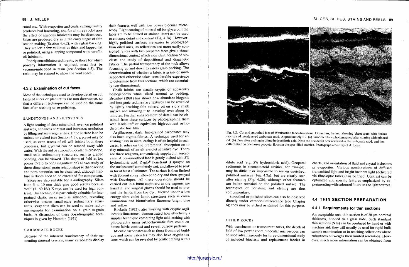
88 J . MILLER
4.3.2 Examination of cut faces
Most of the techniques used to develop detail on cut faces of slices or plaquettes are non-destructive, so that a different technique can be used on the same face after washing or fe-polishing.
S A N D S T O N E S A N D S I L T S T O N E S
A light coating of clear mineral oil, even on polished surfaces, enhances contrast and increases resolution by filling surface irregularities. If the surface is to be stained or etched (see Section 4.5) , glycerol may be used, as even traces of oil will inhibit both these processes, but glycerol can be washed away with water . With the aid of a zoom binocular microscope, small-scale sedimentary structures, such as graded bedding, can be viewed. The depth of field at low power ( x l . 5 to x 2 0 magnification) allows study of three-dimensional grain relationships so that packing and pore networks can be visualized, although fracture surfaces need to be examined for comparison.
Slices are also suitable for X-radiography. Slices from 3 to 10 mm thick give good results because 'soft' (5—50 kV) X-rays can be used for high contrast. This technique is particularly valuable for finegrained clastic rocks such as siltstones, revealing otherwise unseen small-scale sedimentary structures . Very thin slices can be used to make radio-micrographs for examination on a grain-to-grain basis. A discussion of these X-radiographic techniques is given by Hamblin (1971).
C A R B O N A T E R O C K S
Because of the inherent translucency of their cementing mineral crystals, many carbonates display
their features well with low power biocular microscopy. Light coating of mineral oil (or glycerol if the faces are to be etched or stained later) can be used to enhance detail and contrast (Fig. 4.2a). However , highly polished surfaces are easier to photograph than oiled ones , as reflections are more easily controlled. Slices with two prepared faces give a three-dimensional context which aids identification of bio-clasts and study of depositional and diagenetic fabrics. The partial t ransparency of the rock allows focussing up and down to assess grain packing. T h e determinat ion of whether a fabric is grain- or mud-supported otherwise takes considerable experience to determine from thin sections, which are essentially two-dimensional.
Chalk fabrics are usually cryptic or apparently homogeneous when sliced normal to bedding. Bromley (1981) has shown how abundant biogenic and inorganic sedimentary textures can be revealed by lightly brushing thin mineral oil on a dry chalk surface and allowing it to 'develop ' over about 30 minutes. Fur ther enhancement of detail can be obtained from these surfaces by photographing them with Kodalith® or equivalent high-contrast or tho-chromatic line film.
Argil laceous, dark , fine-grained carbonates may also have cryptic fabrics. A technique used for revealing flaws in metal casings is often helpful in such cases. It relies on the preferential absorpt ion on to clay minerals of an ultra-violet sensitive dye. The re are three reagents , conveniently supplied in aerosol cans. A pre-smoothed face is gently etched with 5 % hydrochloric acid. Zyglo® Penet ran t is sprayed on the surface until completely wet , and allowed to soak in for at least 10 minutes . T h e surface is then flushed with Solvent spray, allowed to dry and then sprayed with Developer . All these operat ions should be carried out in a fume cupboard as the vapours are harmful, and surgical gloves should be used to protect the hands from the dye. Viewed under a low energy ultra-violet lamp, structures such as cross-lamination and bioturbation fluoresce bright blue and yellow.
Bockelie (1973), also working with cryptic argillaceous l imestones, demonstra ted how effectively a simpler technique combining light acid etching with photography using or thochromat ic film could enhance fabric contrast and reveal burrow pat terns .
Micritic carbonates such as those from mud buildups and some calcretes may also have cryptic textures which can be revealed by gentle etching with a
1
SLICES, SLIDES, STAINS AND PEELS 89
Fig. 4.2. Cut and smoothed face of Waulsortian facies limestone, Dinantian, Ireland, showing 'sheet spars' with fibrous calcite and interlayered carbonate mud. Approximately x2. (a) Smoothed face photographed after coating with mineral oil. (b) Face after etching in dilute hydrochloric acid. Note the fine detail now revealed in the carbonate mud, and the differentiation of coarser geopetal floors in the spar-filled cavities. Photographs courtesy of A. Lees.
dilute acid (e.g. 5 % hydrochloric acid). Geopeta l sediments in stromatactoid cavities, for example, may be difficult or impossible to see on unetched, polished surfaces (Fig. 4.2a) , but are clearly seen after etching (Fig. 4.2b), although other features are bet ter revealed on the polished surface. T h e techniques of polishing and etching are thus complimentary.
Smoothed or polished slices can also be observed directly under cathodoluminescence (see Chapter 6); they may be etched or stained for this purpose.
O T H E R R O C K S
With translucent or t ransparent rocks, the depth of field of low power zoom binocular microscopes can be used advantageously for three-dimensional study of included bioclasts and replacement fabrics in
cherts , and orientation of fluid and crystal inclusions in evapori tes. Various combinations of diffused transmitted light and bright incident light (delivered via fibre-optic tubes) can be tried. Contrast can be optimized and specific features emphasized by experimenting with coloured filters on the light sources.
4.4 T H I N S E C T I O N P R E P A R A T I O N
4.4.1 Requirements for thin sections
A n acceptable rock thin section is of 30 pm nominal thickness, bonded to a glass slide. Such s tandard thin sections (STs) can be produced by hand or with machine aid: they will usually be used for rapid bulk sample examination or in teaching collections where robustness outweighs their limited resolution. However, much more information can be obtained from
iiiiiiiimmiHiiiiiiiimi
cated saw. With evaporites and coals, cutting usually produces bad fracturing, and for all th ree rock-types the effect of aqueous lubricants may be disastrous. Slices are produced dry as in the early stages of thin section making (Section 4.4.2) , with a glass backing. They are left a few millimetres thick and lapped flat or polished, using a lapping compound with paraffin oil lubricant.
Poorly consolidated sediments , or those for which porosity information is required, must first be vacuum-imbedded in resin (see Section 4.5) . The resin may be stained to show the void space.
http://jurassic.ru/
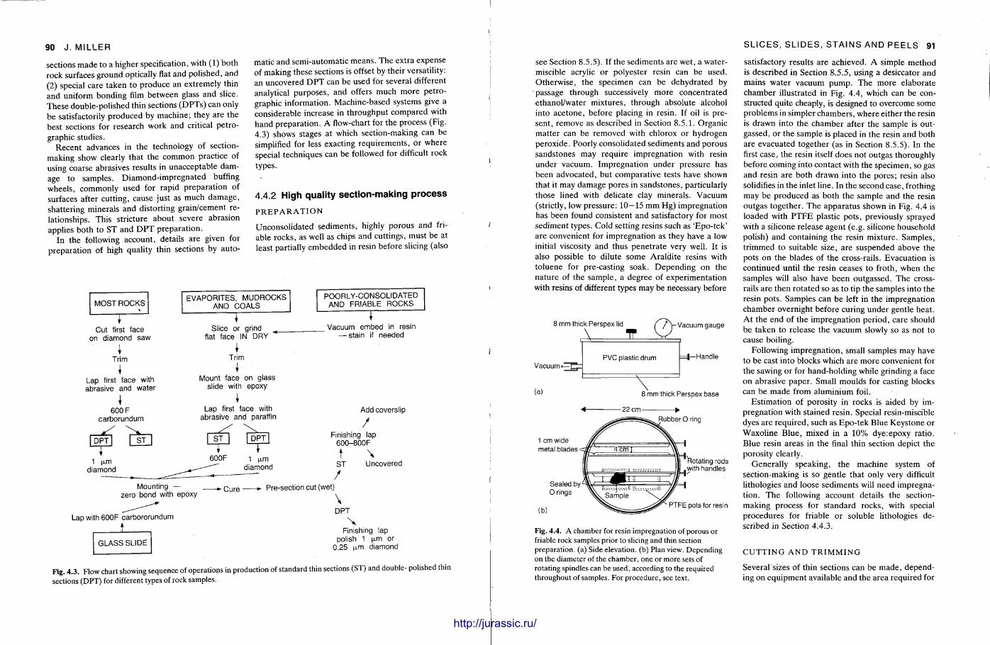
90 J . MILLER
sections made to a higher specification, with (1) both rock surfaces ground optically flat and polished, and (2) special care taken to produce an extremely thin and uniform bonding film between glass and slice. These double-polished thin sections (DPTs) can only be satisfactorily produced by machine; they a re the best sections for research work and critical pe t rographic studies.
Recent advances in the technology of section-making show clearly that the common practice of using coarse abrasives results in unacceptable damage to samples. Diamond- impregnated buffing wheels, commonly used for rapid prepara t ion of surfaces after cutting, cause just as much damage , shattering minerals and distorting grain/cement relationships. This stricture about severe abrasion applies both to ST and D P T preparat ion.
In the following account, details are given for prepara t ion of high quality thin sections by auto
matic and semi-automatic means . The extra expense of making these sections is offset by their versatility: an uncovered D P T can be used for several different analytical purposes , and offers much more pet rographic information. Machine-based systems give a considerable increase in throughput compared with hand preparat ion. A flow-chart for the process (Fig. 4.3) shows stages at which section-making can be simplified for less exacting requi rements , or where special techniques can be followed for difficult rock types.
4.4.2 High quali ty sect ion-making process
P R E P A R A T I O N
Unconsolidated sediments , highly porous and friable rocks, as well as chips and cuttings, must be at least partially embedded in resin before slicing (also
MOST ROCKS
1 Cut first face
on diamond saw
\ Trim I
Lap first face with abrasive and water I
600 F carborundum
DPT
T ST
1 (i.m diamond
Mounting -zero bond with
EVAPORITES, MUDROCKS AND COALS
r Slice or grind
flat face IN DRY
I Trim I
Mount face on glass slide with epoxy
\ Lap first face with
abrasive and paraffin
ST DPT
600F 1 u.m diamond
POORLY-CONSOLIDATED AND FRIABLE ROCKS
Vacuum embed in resin — stain if needed
Add coverslip
/ Finishing lap
600-800F
t \ ST Uncovered /
epoxy - Cure »• Pre-section cut (wet)
Lap with 600F carbororundum
t . GLASS SLIDE
\ DPT
Finishing lap polish 1 u.m or
0.25 ixm diamond
Fig. 4 .3. Flow chart showing sequence of operations in production of standard thin sections (ST) and double- polished thin sections (DPT) for different types of rock samples.
I i i fffffffffffffffffff|f
SLICES, SLIDES, STAINS AND PEELS 91
see Section 8.5.5). If the sediments are wet , a water-miscible acrylic or polyester resin can be used. Otherwise, the specimen can be dehydrated by passage through successively more concentrated ethanol/water mixtures, through absolute alcohol into ace tone , before placing in resin. If oil is present, remove as described in Section 8.5.1. Organic matter can be removed with chlorox or hydrogen peroxide. Poorly consolidated sediments and porous sandstones may require impregnation with resin under vacuum. Impregnat ion under pressure has been advocated, but comparat ive tests have shown that it may damage pores in sandstones, particularly those lined with delicate clay minerals. Vacuum (strictly, low pressure: 10—15 mm Hg) impregnation has been found consistent and satisfactory for most sediment types. Cold setting resins such as 'Epo- tek ' are convenient for impregnation as they have a low initial viscosity and thus penet ra te very well. It is also possible to dilute some Araldi te resins with toluene for pre-casting soak. Depending on the nature of the sample , a degree of experimentat ion with resins of different types may be necessary before
8 mm thick Perspex lid
Vacuum
(a)
/ V Vacuum gauge
-Handle
8 mm thick Perspex base
-22 cm-Rubber O ring
Sealed by O rings
Rotating rods with handles
PTFE pots for resin
Fig. 4.4. A chamber for resin impregnation of porous or friable rock samples prior to slicing and thin section preparation, (a) Side elevation, (b) Plan view. Depending on the diameter of the chamber, one or more sets of rotating spindles can be used, according to the required throughout of samples. For procedure, see text.
satisfactory results are achieved. A simple method is described in Section 8.5.5, using a desiccator and mains water vacuum pump . The more elaborate chamber illustrated in Fig. 4.4, which can be constructed quite cheaply, is designed to overcome some problems in simpler chambers , where either the resin is drawn into the chamber after the sample is out-gassed, or the sample is placed in the resin and both are evacuated together (as in Section 8.5.5). In the first case, the resin itself does not outgas thoroughly before coming into contact with the specimen, so gas and resin are both drawn into the pores ; resin also solidifies in the inlet line. In the second case, frothing may be produced as both the sample and the resin outgas together . The appara tus shown in Fig. 4.4 is loaded with P T F E plastic pots , previously sprayed with a silicone release agent (e.g. silicone household polish) and containing the resin mixture. Samples, t r immed to suitable size, are suspended above the pots on the blades of the cross-rails. Evacuation is continued until the resin ceases to froth, when the samples will also have been outgassed. The cross-rails are then rotated so as to tip the samples into the resin pots. Samples can be left in the impregnation chamber overnight before curing under gentle heat . At the end of the impregnation period, care should be taken to release the vacuum slowly so as not to cause boiling.
Following impregnat ion, small samples may have to be cast into blocks which are more convenient for the sawing or for hand-holding while grinding a face on abrasive paper . Small moulds for casting blocks can be made from aluminium foil.
Est imation of porosity in rocks is aided by impregnation with stained resin. Special resin-miscible dyes are required, such as Epo- tek Blue Keystone or Waxoline Blue , mixed in a 10% dye:epoxy ratio. Blue resin areas in the final thin section depict the porosity clearly.
General ly speaking, the machine system of section-making is so gentle that only very difficult lithologies and loose sediments will need impregnation. The following account details the section-making process for s tandard rocks, with special procedures for friable or soluble lithologies described in Section 4.4.3.
C U T T I N G A N D T R I M M I N G
Several sizes of thin sections can be made , depending on equipment available and the area required for
I http://jurassic.ru/
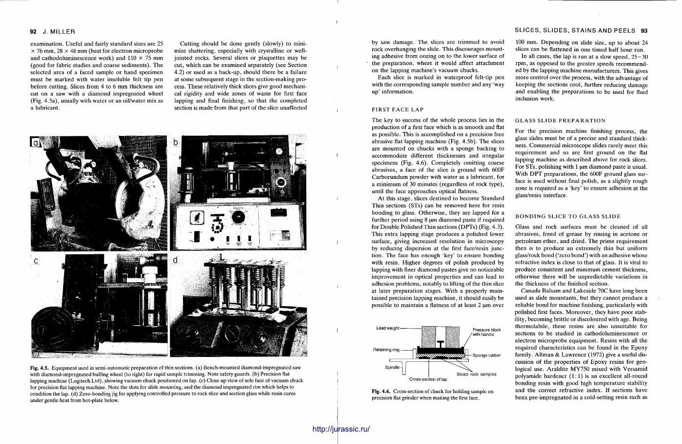
92 J . MILLER
examination. Useful and fairly s tandard sizes are 25 x 76 m m , 28 x 48 mm (best for electron microprobe and cathodoluminescence work) and 110 x 75 mm (good for fabric studies and coarse sediments) . T h e selected area of a faced sample or hand specimen must be marked with water insoluble felt tip pen before cutting. Slices from 4 to 6 mm thickness are cut on a saw with a diamond impregnated wheel (Fig. 4 .5a) , usually with water or an oil/water mix as a lubricant.
Cutt ing should be done gently (slowly) to minimize shattering, especially with crystalline or well-jointed rocks. Several slices or plaquettes may be cut, which can be examined separately (see Section 4.2) or used as a back-up, should there be a failure at some subsequent stage in the section-making process. These relatively thick slices give good mechanical rigidity and wide zones of waste for first face lapping and final finishing, so that the completed section is made from that part of the slice unaffected
Fig. 4 .5. Equipment used in semi-automatic preparation of thin sections, (a) Bench-mounted diamond-impregnated saw with diamond-impregnated buffing wheel (to right) for rapid sample trimming. Note safety guards, (b) Precision flat lapping machine (Logitech Ltd), showing vacuum chuck positioned on lap. (c) Close up view of sole face of vacuum chuck for precision flat lapping machine. Note the slots for slide mounting, and the diamond impregnated rim which helps to condition the lap. (d) Zero-bonding jig for applying controlled pressure to rock slice and section glass while resin cures under gentle heat from hot-plate below.
iiiiimiiiimiiiiiiiwiiii
SLICES, SLIDES, STAINS AND PEELS 93
by saw damage . The slices are t r immed to avoid rock overhanging the slide. This discourages mounting adhesive from oozing on to the lower surface of the prepara t ion, where it would affect a t tachment on the lapping machine 's vacuum chucks.
Each slice is marked in waterproof felt-tip pen with the corresponding sample number and any 'way up ' information.
F I R S T F A C E L A P
The key to success of the whole process lies in the production of a first face which is as smooth and flat as possible. This is accomplished on a precision free abrasive flat lapping machine (Fig. 4.5b). The slices are mounted on chucks with a sponge backing to accommodate different thicknesses and irregular specimens (Fig. 4.6). Completely omitting coarse abrasives, a face of the slice is ground with 600F Carborundum powder with water as a lubricant, for a minimum of 30 minutes (regardless of rock type) , until the face approaches optical flatness.
At this stage, slices destined to become Standard Thin sections (STs) can be removed here for resin bonding to glass. Otherwise , they are lapped for a further period using 8 um diamond paste if required for Doub le Polished Thin sections (DPTs) (Fig. 4.3) . This extra lapping stage produces a polished lower surface, giving increased resolution in microscopy by reducing dispersion at the first face/resin junction. The face has enough 'key' to ensure bonding with resin. Higher degrees of polish produced by lapping with finer d iamond pastes give no noticeable improvement in optical propert ies and can lead to adhesion problems, notably to lifting of the thin slice at later preparat ion stages. With a properly maintained precision lapping machine, it should easily be possible to maintain a flatness of at least 2 um over
Lead weight Pressure block with handle
Sponge rubber
Cross-section of lap Sliced rock samples
Fig. 4.6. Cross-section of chuck for holding sample on precision flat grinder when making the first face.
100 mm. Depending on slide size, up to about 24 slices can be flattened in one t imed half hour run.
In all cases, the lap is run at a slow speed, 25—30 rpm, as opposed to the greater speeds recommended by the lapping machine manufacturers . This gives more control over the process, with the advantage of keeping the sections cool, further reducing damage and enabling the preparat ions to be used for fluid inclusion work.
G L A S S S L I D E P R E P A R A T I O N
For the precision machine finishing process, the glass slides must be of a precise and standard thickness. Commercial microscope slides rarely meet this requirement and so are first ground on the flat lapping machine as described above for rock slices. For STs, polishing with 1 um diamond paste is usual. With D P T preparat ions , the 600F ground glass surface is used without final polish, as a slightly rough zone is required as a 'key ' to ensure adhesion at the glass/resin interface.
B O N D I N G S L I C E T O G L A S S S L I D E
Glass and rock surfaces must be cleaned of all abrasives, freed of grease by rinsing in acetone or pet roleum ether , and dried. T h e prime requirement then is to produce an extremely thin but uniform glass/rock bond ( 'zero bond ' ) with an adhesive whose refractive index is close to that of glass. It is vital to produce consistent and minimum cement thickness, otherwise there will be unpredictable variations in the thickness of the finished section.
Canada Balsam and Lakeside 70C have long been used as slide mountants , but they cannot produce a reliable bond for machine finishing, particularly with polished first faces. Moreover , they have poor stability, becoming brittle or discoloured with age. Being thermolabi le , these resins are also unsuitable for sections to be studied in cathodoluminescence or electron microprobe equipment . Resins with all the required characteristics can be found in the Epoxy family. Al lman & Lawrence (1972) give a useful discussion of the propert ies of Epoxy resins for geological use. Araldi te MY750 mixed with Versamid polyamide hardener (1 :1 ) is an excellent all-round bonding resin with good high tempera ture stability and the correct refractive index. If sections have been pre- impregnated in a cold-setting resin such as
http://jurassic.ru/
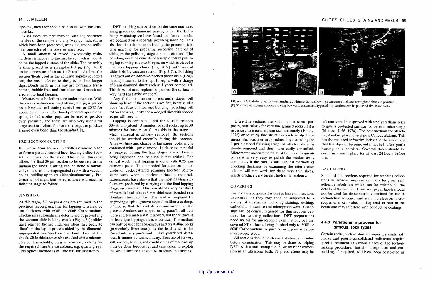
94 J . MILLER
Epo- tek , then they should be bonded with the same material .
Glass sides are first marked with the specimen number of the sample and any 'way u p ' indications which have been preserved, using a d iamond scribe near one edge of the obverse glass face.
A small amount of mixed low-viscosity resin/ hardener is applied to the first face, which is mounted on the lapped surface of the slide. The assembly is then placed in a spring-loaded jig (Fig. 4.5d) under a pressure of about 1 k G c m - 2 . At first, the section 'floats', but as the adhesive rapidly squeezes out , the rock locks on to the glass and no longer slips. Bonds made in this way are extremely transparent , bubble-free and introduce no dimensional errors into final lapping.
Mounts must be left to cure under pressure. With the resin combination used above , the jig is placed on a hotplate and curing carried out at 80°C for about 15 minutes. For hand-prepared specimens, spring-loaded clothes pegs can be used to provide even pressure, and these are also .very useful for large sections, where four or more pegs can produce a more even bond than the s tandard jig.
P R E - S E C T I O N G U T T I N G
Bonded sections are next cut with a d iamond blade to form a parallel second face, leaving a slice 300— 400 um thick on the slide. This initial thickness allows the final 30 um section to be entirely in the undamaged layer. Cutt ing can be done automatically on a diamond-impregnated saw with a vacuum chuck, holding up to six slides simultaneously. Precision is not important here , as there is a machine finishing stage to follow.
F I N I S H I N G
At this stage, ST preparat ions are re turned to the precision lapping machine for lapping to a final 30 um thickness with 600F or 800F Carborundum. Thickness is automatically determined by pre-setting the vacuum slide-holding chuck (Fig. 4.5c); slides have reached the set thickness when they begin to 'float' on the lap, a process aided by the diamond-impregnated surround on the lower face of the chuck. Slide thickness can be checked with a micrometer or, less reliably, on a microscope, looking for the required interference colours, e.g. quartz greys. This optical method is of little use for l imestones.
D P T polishing can be done on the same machine, using graduated diamond pastes, but in the Edinburgh workshop we have found that bet ter results are obtained on a separate polishing machine. This also has the advantage of freeing the precision lapping machine for preparing successive batches of slides, as the polishing stage can be protracted. The polishing machine consists of a simple rotary polishing lap running at up to 30 rpm, on which is placed a precision lapping chuck (Fig. 4.7a) with several slides held by vacuum suction (Fig. 4 .7b) . Polishing is carried out on adhesive-backed paper discs (Engis papers) at tached to the lap. It begins with a charge of 8 um diamond slurry such as Hyprez compound . This does not need replenishing unless the surface is very hard (quartzite or chert) .
Any faults in previous preparat ion stages will show up here : if the section is not flat, because of a poor first face or incorrect bonding, polishing will follow the irregularity and a wedged slice with eroded edges will result.
Lapping is continued until the section reaches 30—35 um (about 10 minutes for soft rocks, up to 30 minutes for harder ones) . As this is the stage at which material is actively removed, the sections should be watched carefully during this process. After washing and change of lap paper , polishing is continued with 1 um diamond. Little or no material is removed during the final stages; the surface is being improved and so time is not critical. For critical work, final lapping is done with 0.25 um diamond paste. This is needed for electron microprobe or back-scattered Scanning Electron Microscope work where a perfect surface is required. Exper iments have shown that the most flawless surfaces are produced by carrying out the final lapping stages on a lead lap. This consists of a very flat sheet of metallic lead, about 8 mm thickness, bonded to a s tandard steel lap disc. The lead is prepared by engraving a spiral groove several millimetres d e e p , pitched so that the lead strip is narrower than the groove. Sections are lapped using paraffin oil as a lubricant. N o material is removed, but the surface is perfected, so lapping time is not critical. This method can only be used for non-porous and crystalline rocks (particularly l imestones) , as the lead tends to be forced into any pores and, unlike powdered abrasives, it cannot be washed away. Because of its very soft surface, trueing and conditioning of the lead lap must be done frequently, and care taken to exploit the whole surface to avoid worn spots and dishing.
SLICES, SLIDES, STAINS AND PEELS 95
Fig. 4.7. (a) Polishing lap for final finishing of thin sections, showing a vacuum chuck and a weighted chuck in position, (b) Sole face of vacuum chucks showing how various sizes and types of thin sections can be polished simultaneously.
Ultra-thin sections are valuable for some purposes, particularly for very fine grained rocks, if it is necessary to measure grain size accurately (Halley, 1978) or to study fine structures such as algal filaments . Such sections are produced by extending the 1 um diamond finishing stage, at which material is slowly removed and thus more easily controlled. Micrometer measurements must be made frequently, as it is very easy to polish the section away completely if the rock is soft. Optical methods of checking thickness by examining the interference colours will not work for these very thin slices, which produce very bright, high order colours.
C O V E R I N G
For research purposes it is best to leave thin sections uncovered, as they may then be subjected to a variety of t reatments including staining, etching, cathodoluminescence and microprobe work. Cover-slips a re , of course, required for thin sections destined for teaching collections. D P T preparat ions need no oil for microscopic examination, but uncovered ST surfaces, being finished only to 600F or 800F Carborundum, require oil or glycerine before microscopic study.
All sections should be cleaned of abrasive residue before examinat ion. This may be done by wiping DPTs with a soft, damp tissue, or by brief immersion in an ultrasonic bath. ST preparat ions may be
left uncovered but sprayed with a polyurethane resin to give a protected surface for general microscopy (Moussa, 1976, 1978). The best medium for attaching standard glass coverslips is Canada Balsam. This has the required refractive index and the advantage that the slip can be removed if needed , after gentle heating on a hotpla te . Covered slides should be cured in a warm place for at least 24 hours before use.
L A B E L L I N G
Standard thin sections required for teaching collections or archive purposes can now be given self-adhesive labels on which can be written all the details of the sample. However , paper labels should not be used for those sections destined for use in cathodoluminescence and scanning electron microscopes or microprobe, as they tend to char in the beam and may interfere with conductive coatings.
4.4.3 Variations in process for 'diff icult ' rock types
Certain rocks, such as shales, evapori tes, coals, soft chalks and poorly-consolidated sediments require special t rea tment at various stages of the section-making procedure . Initial impregnation and embedding, if required, will have been completed as
http://jurassic.ru/
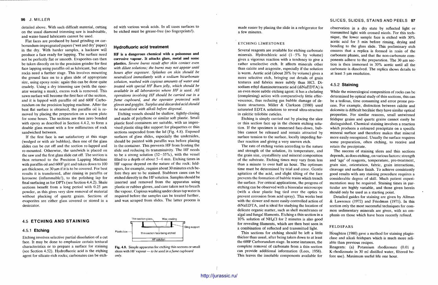
96 J . MILLER
detailed above. With such difficult mater ia l , cutting on the usual d iamond tr imming saw is inadvisable, and water-based lubricants cannot be used.
Flat faces are produced by hand grinding on carborundum-impregnated papers ( 'wet and dry' paper ) in the dry. With harder samples, a hacksaw will produce a face ready for lapping. The surface need not be perfectly flat or smooth. Evapori tes can then be taken directly on to the precision grinder for first face lapping using paraffin oil as lubricant, but o ther rocks need a further stage. This involves mount ing the ground face on to a glass slide of appropr ia te size, using epoxy resin: again this can be done quite crudely. Using a dry tr imming saw (with the operator wearing a mask) , excess rock is removed. This sawn surface will become the first face of the section, and it is lapped with paraffin oil and 600F Carborundum on the precision lapping machine. After the best flat surface is obta ined, the paraffin oil is removed by placing the preparat ion on a warm plate for some hours . T h e sections are then zero bonded with epoxy as described in Section 4 .4 .2 , to form a double glass mount with a few millimetres of rock sandwiched between.
If the first face is not satisfactory at this stage (wedged or with air bubbles) , then one of the glass slides can be cut off and the section re-lapped and re-mounted. Otherwise , the sandwich is placed on the saw and the first glass slide cut off. T h e section is then returned to the Precision Lapping Machine with paraffin oil and 600F grit and taken down to 100 urn thickness, or 30 um if it is to be covered. For best results it is t ransferred, after rinsing in paraffin or kerosene (inflammable!), to the polishing lap for final surfacing as for D P T s (see Section 4.4.2). Shale sections benefit from a long period with 0.25 um powder , as this gives very slow removal of material without plucking of quartz grains. Sections of evaporites are either glass covered or stored in a desiccator.
ed with various weak acids. In all cases surfaces to be etched must be grease-free (no fingerprints!).
Hydrofluoric acid treatment
HF is a dangerous chemical with a poisonous and corrosive vapour. It attacks glass, metal and some plastics. Severe burns result after skin contact even with dilute solutions; the burns may not appear until hours after exposure. Splashes on skin should be neutralized immediately with a sodium bicarbonate solution, washed with copious amounts of water and treated with special HF Burn jelly, which should be available in all laboratories where HF is used. All operations involving HF should be carried out in a fume cupboard, and the operator protected with gloves and goggles. Surplus and discarded acid should be neutralized with alkali before disposal.
Etching vessels should be shallow, tightly-closing and made of polythene or similar soft plastic. Small plastic food containers are suitable, with an improvised plastic sling-like support for plaquettes or thin sections suspended from the lid (Fig. 4.8) . Exposed surfaces of glass slides, especially the unders ides , should be painted with paraffin wax before placing in the container . This prevents H F from frosting the slide and reducing its transmissivity. T h e H F needs to be a strong solution (52—55%), with the vessel filled to a depth of about 5—6 mm. Etching t imes in H F vapour depend on the nature of the rock: feldspars, for example , require about 30 minutes etch before they are to be stained. Stubborn cases can be etched directly in the H F solution. Samples should be inserted and removed from the appara tus using plastic or rubber gloves, and care taken not to breath the vapour . Copious washing under clean tap water is required before the samples can be t rea ted further, and wax scraped from slides. T h e latter process is
4.5 E T C H I N G A N D S T A I N I N G
4.5.1 Etching
Etching involves selective partial dissolution of a cut face. It may be done to emphasize certain textural characteristics or to prepare a surface for staining (see Section 4.52). Hydrofluoric acid is the etching agent for silicate-rich rocks; carbonates can be etch-
Thin section glass
Plastic box -
1 V Wax coating
Thin section face being etched
HF solution
Sling support
Fig. 4.8. Simple apparatus for etching thin sectons or small slices with HF vapour — to be used in a fume cupboard only.
i II
SLICES, SLIDES, STAINS AND PEELS 97
made easier by placing the slide in a refrigerator for a few minutes.
E T C H I N G L I M E S T O N E S
Several reagents are available for etching carbonate minerals. Hydrochloric acid (1—5% by volume) gives a vigorous reaction with a tendency to give a ra ther unselective etch. It affects minerals other than calcite and aragoni te , especially if the solution is warm. Acetic acid (about 2 0 % by volume) gives a more selective etch, bringing out details of grain textures and fabrics m o r e subtly than HC1. Di-sodium ethyl diaminotetracetic acid ( d i N a E D T A ) is an even more subtle etching agent: it has a chelating (complexing) action with comparatively little effervescence, thus reducing gas bubble damage of delicate structures. Miller & Clarkson (1980) used saturated E D T A solutions to reveal ultra-structure in calcitic trilobite cuticles.
Etching is simply carried out by placing the slice or thin section face up in the chosen etching solution. If the specimen is immersed face-down, bubbles cannot be released and remain at tracted by surface tension to the surface, locally impeding further reaction and giving a very uneven etch.
The rate of etching varies according to the nature and strength of the solution, its t empera ture , and the grain size, crystallinity and mineral composition of the substrate. Etching t imes may vary from less than a minute to over half an hour . The opt imum time must be determined by trial and error . Gent le agitation of the acid, and slight tilting of the face prevents the formation of bubble trains which trench the surface. For critical applications, the progress of etching can be observed with a binocular microscope (with a clear plastic bag tied over the optics to prevent corrosion from acid spray). This works best with t he slower and more easily-controlled action of d i N a E D T A , and is ideal for studying the location of delicate organic mat ter , such as shell membranes or algal and fungal filaments. Etching a thin section in a 10% solution of N H 4 C 1 for 2 minutes is also good for revealing filaments, which a re then best seen in a combinat ion of reflected and transmitted light.
Thin sections for etching should be left a little thicker than usual , after being taken down to at least the 600F Carborundum stage. In some instances, the complete removal of carbonate from a thin section can provide additional information (Lees, 1958). This leaves the insoluble components available for
observation in a dry state by reflected light or t ransmit ted light with crossed nicols. For this technique, the lower sample face is etched with 3 0 % acetic acid for 5 min before rinsing, drying and bonding to the glass slide. This preliminary etch ensures that a replica is formed in resin of the carbonate phases, and that the non-carbonate components adhere to the preparat ion. The 30 um section is then immersed in 30% acetic until all the carbonate is dissolved. The replica shows details to at least 5 um resolution.
4.5.2 Staining
While the mineralogical composit ion of rocks can be determined by optical study of thin sections, this can be a tedious, t ime consuming and error prone process. For example , distinction between calcite and dolomite is difficult because they have similar optical propert ies . For similar reasons, small untwinned feldspar grains and quar tz grains cannot easily be distinguished. Chemical staining involves a reaction which produces a coloured precipitate on a specific mineral surface and therefore makes that mineral more easily recognized. Usually the surface requires some prepara t ion , often etching, t o receive and retain the precipitate.
The success of staining slices and thin sections depends , as does etching, on various factors: strength and 'age ' of reagents , t empera tu re , pre- t rea tment , grain size, or ientat ion, fabric, grain interactions, cleavage and surface finish. To achieve consistently good results with any staining procedure requires a considerable degree of skill. Much patient experimentat ion may be required. Staining times in particular are highly variable, and those given herein should only be used as a starting point.
Detai led guides for staining are given by Allman & Lawrence (1972) and Fr iedman (1971). In this section only the most successful techniques for common sedimentary minerals are given, with an emphasis on those which have been recently refined.
F E L D S P A R S
Houghton (1980) gave a method for staining plagio-clase and alkali feldspars which is much more reliable than previous recipes. Reagents : (a) Potassium rhodizonate (0.01 g K-rhodizonate in 30 ml distilled water , filtered before use) . Maximum useful life one hour .
http://jurassic.ru/

98 J . MILLER
(b) Sodium cobaltinitrate (saturated solution; about 50 g per 100 ml distilled water ) . Six months shelf life in dark bottle. (c) Barium chloride ( 5 % solution in distilled water ) . Stable. Procedure : (a) Etch over H F vapour (55% H F solution, see Section 4.5.1) for 2 5 - 3 5 s: increase t ime if H F is loosing potency. (b) Remove slide from etching box with polythene forceps and drop into beaker with Na-cobalt initrate solution. Leave for 45 s. (c) Rinse slide twice in distilled or de-ionized water . Gently shake off excess water and blot end of slide by touching to a paper towel. (d) Dip slide quickly into beaker with B a C l 2 solution for no more than 2 s. (e) Dip slide immediately in distilled water and agitate for about 10 s. (f) Place several drops of the rhodizonate solution on the wet surface of the section, tilting back and forth to spread the stain; leave until plagioclase grains become pink, then rinse in water . (g) Dry with compressed air and examine with a microscope. If plagioclase is light grey or pale pink, dip in distilled water and* repeat rhodizonate stage. The intensity of the pink plagioclase stain is proportional to the amount of calcium in the molecule: albite/oligoclase will stain lighter than a more calcic plagioclase. Pure Na-albite will not take up any of the rhodizonate stain. Alkali feldspars are stained yellow. T h e accuracy of the method decreases according to grain size: with finer grained specimens, the pink stain tends to pervade the surface and obscure the quartz grains.
Cathodoluminescence is a much bet ter way of detecting feldspars in fine sands and siltstones (see Chapter 6) .
G Y P S U M A N D A N H Y D R I T E
Hounslow (1979) gave a method for staining these minerals , useful in the field as well as on drill cores , soil samples, slabs and sections. Reagents : (a) 1:1 nitric acid solution (10 ml concentrated nitric acid slowly added to 10 ml water in a 50 ml beaker ) . (b) 10 g mercuric ni trate in 100 ml de-ionized water . Stir until dissolved. A fine, milky precipitate will form. Caution! Mercuric ni trate is extremely poisonous and may be absorbed through the skin. (c) Slowly add the 1:1 nitric acid to the mercuric
nitrate with constant stirring until the milky precipitate just dissolves or is just about to — approximately 8 drops of acid is usually sufficient. (d) Test the reagent by adding a few drops to small crystals of N a 2 S 0 4 or K 2 S 0 4 in a watch glass. A yellow precipitate should form immediately. If not , the reagent is too acid and a further gram of mercuric nitrate added to produce a slight cloudiness should produce the yellow precipitate. (e) Filter the solution when the test is successful and store in a dark bot t le . Procedure : (a) Immerse the section, slab or pla-quet te in the reagent contained in a suitable dish or tray for a few seconds or until the yellow precipitate forms. (b) Gently rinse the stained face in de-ionized or distilled water and allow to dry before microscopic examination. Both minerals are stained yellow; other minerals are unstained.
A R A G O N I T E
The most sensitive stain for aragonite was developed by Fiegl (1937). Despi te its sensitivity, it is not always reliable. Reagents : (a) 1 g commercial grade A g 2 S 0 4 is added to a boiling solution of 11.8 g M n S O 4 . 7 H 2 0 in 100 ml distilled water . (b) Cool and filter the suspension; add 2 drops 10% sodium hydroxide solution. (c) Stand for 2 hours and then filter into a dark storage bott le . Procedure : Immerse the plaquet te or thin section in the Fiegl's solution for about 10 min at 20°C. Sometimes a hot solution works bet ter . Aragoni te is stained black while calcite remains unstained.
D O L O M I T E
Dolomi te is often distinguished from calcite by its failure to stain with solutions which react with calcite (see below). It can also be recognized after etching, especially on a universal stage: dolomite remains at 30 um, giving fourth- and fifth-order pinks and greens, while calcite is reduced to 10 um or so , giving second- and third-order reds , blues and yellows (Dickson, 1966, p . 491). Titan yellow in alcohol and alkaline Alizarin red S are two reliable
SLICES, SLIDES, STAINS AND PEELS 99
specific stains for dolomite , but have the disadvantage for thin sections of needing to boil.
Ti tan yellow — reagent: (a) 0.2 g Titan yellow is dissolved in 25 ml methanol in a small beaker over a hot water bath. Replace any alcohol lost by evaporat ion. (b) 30 g sodium hydroxide pellets dissolved cautiously in 70 ml distilled water.
Ti tan yellow — procedure : (a) Add 15 ml of the 3 0 % N a O H solution to the Titan yellow solution and bring to the boil. (b) Immerse the thin section or plaquet te in boiling Titan yellow reagent for at least 5 min until a deep orange-red colouration is formed. Add a few drops of methanol to compensate for evaporat ion.
Alkal ine Alizarin red S — reagent: (a) Dissolve 0.2 g Alizarin red S in 25 ml methanol in a small beaker over a hot water bath , (b) Carefully dissolve 30 g sodium hydroxide pellets in 70 ml water .
Alkaline Alizarin red — procedure : (a) A d d 15 ml of the 30% N a O H solution to the Alizarin red solution and bring to the boil. (b) Immerse the section or plaquet te in boiling reagent for at least five minutes . Add a few drops of methanol to compensate for evaporat ion. (c) Rinse the section in distilled water . Dolomi te is stained purple , calcite is unstained in the alkaline solution.
M G - C A L C I T E
Choque t te & Trusell (1978) devised a method of making an alkaline Titan yellow stain permanent , enhancing the value of this technique. The stain can detect the presence of Mg-calcite containing more than about 3 % M g C 0 3 . Reagents : (a) Stain: 1.0 g Titan yellow powder , 8.0 g N a O H and 4.0 g d i N a E D T A dissolved in 1 litre distilled water at room tempera ture . Store in dark bot t le ; shelf life at least two years, (b) Fixer: 200 g N a O H pellets dissolved slowly in 1.0 litre distilled water . Caution! heat and fumes and evolved, so best carried out in fume cupboard. Solution is corrosive to flesh. Store in polythene bottles as 5 M caustic soda etches glass. Shelf life indefinite. Procedure (Caution! use surgical gloves as solutions are corrosive): (a) Thin sections must be epoxy mounted : Lakeside and Canada Balsam are soluble in the stain solution.
(b) Etch uncovered, grease-free thin section or faced sample for about 30 s in 5 % acetic acid solution. (c) Dry surface in s tream of warm air. (d) Immerse specimen in stain solution for about 20 min. (e) Dry stained surface in s tream of warm air; do not touch surface in any way. (f) Immerse stained surface in fixer solution for about 30 s. (g) Air dry again and cover. As the residual caustic would attack Lakeside or Canada Balsam, epoxy cement is required for cover slips. Choquet te & Trusell (1978) found that the intensity of the stain was proport ional to the Mg content of calcite. Calcite with 5—8% M g C 0 3 takes on a pink to pale red colour, and 'high-Mg' calcite takes on a deep red colour, c-axis normal sections of crystals stain more vividly than parallel sections, as d o very fine-grained substrates. This stain is very valuable for its minute selectivity on a scale discernible with a petrographic microscope.
C A L C I T E
Friedman (1959) gave a number of stains for calcite. O n e of the simplest and most reliable is Alizarin red S. Many carbonate workers routinely acid etch one-half of a thin section and stain it in acidified Alizarin red S solution before covering. While this helps to distinguish between red-stained calcite and unstained dolomite and quar tz , it gives very little o ther information about diagenesis and mineralogy. It also makes microphotography of that slide difficult. A far m o r e valuable scheme was given by Dickson (1965, 1966) which in one operat ion differentiates between ferroan phases in calcites and dolomites, and is capable of revealing subtle growth zones in cement crystals.
Dickson's method — reagents: (a) Etching solution — 15 ml of 36% HC1 dissolved in 500 ml distilled water , then topped up to 1000 ml with distilled water . (b) Staining solution part 1:0.2 g Alizarin red S dissolved in 100 ml 1.5% HC1 solution. (c) Staining solution part 2 : 2 g potassium ferri-cyanide crystals dissolved in 100 ml 1.5% HC1 solution. This solution must be freshly made for each staining session. (d) Mix staining solutions parts 1 and 2 in the ratio 3 of dye t o 2 ferricyanide. T h e combined solution lasts for only one staining session.
http://jurassic.ru/
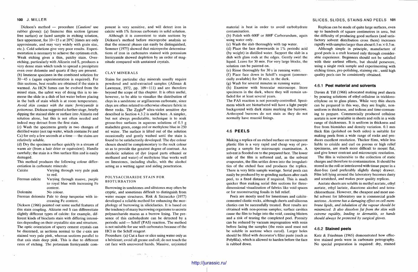
100 J . MILLER
Dickson's method — procedure (Caution! use rubber gloves): (a) Immerse thin section (grease free surface) or faced sample in etching solution, face uppermost , for 10—15 s at 20°C (times are only approximate , and may vary widely with grain size, e tc . ) . Cold solutions give very poor results. Experimentat ion is necessary to achieve the op t imum etch. Weak etching gives a thin, patchy stain. Over-etching, particularly with Alizarin red S, produces a very dense stain which tends to spread a precipitate even over dolomite and quartz if they are present . (b) Immerse specimen in the combined solution for 30—45 s (again experimentat ion is requi red) . For thin sections, best results are obtained if the stain is warmed. As H C N fumes can be evolved from the mixed stain, the safest way of doing this is to immerse the slide in a dish of hot water before placing in the bath of stain which is at room tempera tu re . Avoid skin contact with the stain: ferricyanide is poisonous. Dickson suggested a further s tage, briefly dipping the stained slide or surface into Alizarin red solution alone, but this is not often needed and indeed may detract from the first stain. (c) Wash the specimens gently in two changes of distilled water (not tap water , which contains Fe and Ca) for only a few seconds at a t ime — the stains are relatively soluble. (d) Dry the specimen surface quickly in a stream of warm air (from a hair drier or equivalent) . Hand le carefully; the stain is a thin surface film and is easily damaged. This method produces the following colour differentiation in carbonate minerals: Calcite Varying through very pale pink
to red. Ferroan calcite Varying through mauve , purple
to royal blue with increasing Fe content .
Dolomite No colour. Ferroan dolomite Pale to deep turquoise with in
creasing Fe content . Dickson (1966) pointed out some useful features of this stain coupling. Alizarin red S can differentiate slightly different types of calcite: for example , different kinds of bioclasts stain with differing intensities depending on their crystallite size and structure. The optic orientat ion of sparry cement crystals can be discerned, as sections normal to the c-axis are stained very pale pink, whereas sections parallel to that axis stain deep pink. This is due to different rates of etching. T h e potassium ferricyanide com
ponent is very sensitive, and will detect iron in calcite with 1% ferrous carbonate in solid solution.
Al though it is convenient to stain sections by Dickson's method before microprobe analysis so that the mineral phases can easily be distinguished, Sommer (1975) showed that microprobe determinations of iron in carbonates stained with potassium ferricyanide showed depletion by an order of magnitude compared with unstained crystals.
C L A Y M I N E R A L S
Stains for particular clay minerals usually require powdered and acid-extracted samples (Allman & Lawrence , 1972, pp . 109-111) and are therefore beyond the scope of this chapter . It is often useful, however , to be able to visualize the distribution of clays in a sandstone or argillaceous carbonate , since clays are often related to otherwise obscure fabric in these rocks. The Zyglo® ultra-violet sensitive dye described in Section 4.3.2 is useful here . A simpler, but not always predictable, technique is to soak grease-free surfaces in aqueous solutions of 0.5 g malachite green, congo red or methylene blue in 250 ml water . The surface is lifted out of the solution occasionally and gently washed until the stain is found to be satisfactorily developed: The dye colour chosen should be complementary to the rock colour so as to provide the greatest degree of contrast . A n alcoholic solution of dye (equal parts ethanol or methanol and water) of methylene blue works well on l imestones, including chalks, with the alcohol acting as a wetting agent and aiding penetra t ion.
P O L Y S A C C H A R I D E S T A I N F O R B I O T U R B A T I O N
Burrowing in sandstones and siltstones may often be cryptic, and sometimes difficult to distinguish from water escape structures. Risk & Szczuczko (1977) developed a reliable method for enhancing the morphology of burrowing in siliciclastics. It is based on the tendency of many burrowing organisms to secrete polysaccharide mucus as a burrow lining. The presence of this carbohydrate can be detected by a periodic acid — Schiff (PAS) reaction. The method is not suitable for use with carbonates because of the HC1 in the Schiff reagent . Procedure : (a) Cut a face or slice using water only as a lubricant; avoid all grease and oil; do not touch the cut face with uncovered hands. Massive, unjointed
111111 l i l l l l l i l l
SLICES, SLIDES, STAINS AND PEELS 101
material is best in order to avoid carbohydrate contaminat ion. (b) Polish with 600F or 800F Carborundum, again using water only. (c) Wash the slab thoroughly with tap water. (d) Place the face downwards in 1% periodic acid (by weight) in distilled water . Support the slab in a dish with glass rods at the edges. Gently swirl the liquid. Leave for 30 min. For very large blocks, the solution can be painted on. (e) Rinse thoroughly for 30 s in running water . (f) Place face down in Schiff's reagent (commercially available) for 30 min, in the dark. (g) Wash for several minutes in running water . (h) Examine with binocular microscope. Store specimens in the dark, where they will remain un-faded for at least several years. The P A S reaction is not porosity-controlled. Specimens which are bioturbated will have a light purple background with dark stains marking the burrows. Ar th ropod burrows do not stain as they do not normally have mucoid linings.
4.6 P E E L S
Making a replica of an etched surface on t ransparent plastic film is a very rapid and cheap way of preparing a sample for microscopic examination. A solvent is flooded on to the prepared face. The lower side of the film is softened and, as the solvent evaporates , the film settles down into the irregularities of the etched face and produces the replica. The re is very little sample wastage. Serial peels can easily be produced by re-grinding surfaces after each peel , to a fixed distance if required. This is much quicker than making serial thin sections for three-dimensional visualization of fabrics like void spaces or for reconstructing fossils in full relief.
Peels are mostly used for limestones and calcite-cemented clastic rocks, al though cherts and siliceous elastics can be successfully t reated. Best results are obtained with non-porous samples; surface cavities cause the film to bulge into the void, causing blisters and a risk of tearing the completed peel. Porosity can be reduced by vacuum impregnation with resin before facing the samples (the resin used must not be soluble in acetone when cured) . Larger holes should be filled with decorator ' s filler paste (such as Polyfilla), which is allowed to harden before the face is rubbed down.
Replicas can be made of quite large surfaces, even up to hundreds of square centimetres in area, but the difficulty of producing good surfaces (and satisfactory solvent distribution cross them) increases rapidly with samples larger than about 0.5 m x 0.5 m.
Al though simple in principle, manufacture of good peels is a craft learned only through considerable experience. Beginners should not be satisfied with their earliest efforts, but should persevere , using a single rock sample and experimenting with etching t imes, pre-polishing, staining e tc . , until high quality peels can be consistently obtained.
4.6.1 Peel material and solvents
Davies & Till (1968) advocated making peel sheets by pouring solutions of ethyl cellulose in trichloro-ethylene on to glass plates. While very thin sheets can be prepared in this way, they are fragile, nonuniform in thickness, and tedious and time-consuming to prepare . Commercially produced cellulose acetate is now available in sheets and rolls in a wide range of thicknesses. It is uniform in thickness and free from blemishes and density variation. 0.1 mm thick film (polished on both sides) is suitable for making peels from a wide range of rocks and produces excellent resolution. Thicker films, while less liable to crinkle and curl on porous or high relief specimens, are much more difficult to mount flat, and give lower contrast and microscopic resolution.
The film is vulnerable to the collection of static charges and therefore to contaminat ion. It should be stored in the roll or interleaved with tissue paper in a dust-free (and preferably slightly damp) drawer. Film left lying around the laboratory becomes dusty and scratched, and makes poor quality replicas.
Ace ta te sheets are soluble in methyl aceta te , ethyl acetate , ethyl lactate, diacetone alcohol and tetra-chloroethane. However , the cheapest and most useful solvent for laboratory use is commercial grade acetone. Acetone has a damaging effect on cell membrane lipids, and inhalation of the vapour should be minimized. It also dissolves fat from the skin with extreme rapidity, leading to dermatitis, so hands should always be protected by surgical gloves.
4.6.2 Stained peels
Katz & Fr iedman (1965) demonst ra ted how effective stained peels were in carbonate petrography. No special prepara t ion is required: dry, stained
http://jurassic.ru/
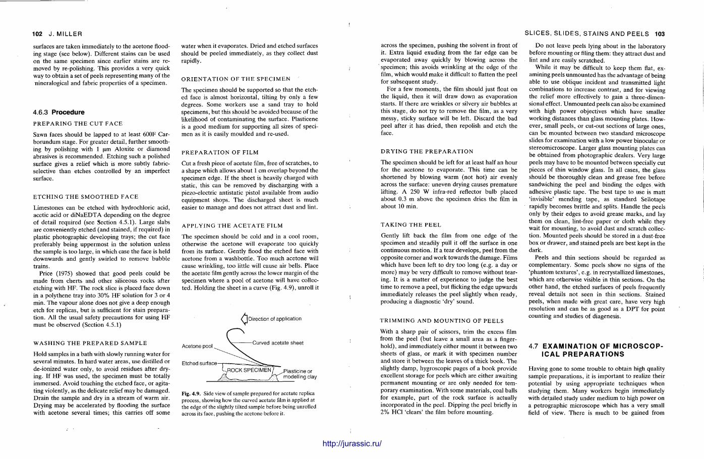
102 J . MILLER
4.6.3 Procedure
P R E P A R I N G T H E C U T F A C E
Sawn faces should be lapped to at least 600F Carborundum stage. For greater detail , further smoothing by polishing with 1 um Aloxite or d iamond abrasives is recommended . Etching such a polished surface gives a relief which is more subtly fabric-selective than etches controlled by an imperfect surface.
E T C H I N G T H E S M O O T H E D F A C E
Limestones can be etched with hydrochloric acid, acetic acid or d i N a E D T A depending on the degree of detail required (see Section 4.5.1). Large slabs are conveniently etched (and stained, if required) in plastic photographic developing trays; the cut face preferably being uppermost in the solution unless the sample is too large, in which case the face is held downwards and gently swirled to remove bubble trains.
Price (1975) showed that good peels could be m a d e from cherts and other siliceous rocks after etching with H F . The rock slice is placed face down in a polythene tray into 30% H F solution for 3 or 4 min. The vapour alone does not give a deep enough etch for replicas, but is sufficient for stain preparation. All the usual safety precautions for using H F must be observed (Section 4.5.1)
water when it evaporates . Dried and etched surfaces should be peeled immediately, as they collect dust rapidly.
O R I E N T A T I O N O F T H E S P E C I M E N
The specimen should be supported so that the etched face is almost horizontal , tilting by only a few degrees. Some workers use a sand tray to hold specimens, but this should be avoided because of the likelihood of contaminat ing the surface. Plasticene is a good medium for supporting all sizes of specimen as it is easily moulded and re-used.
P R E P A R A T I O N O F F I L M
Cut a fresh piece of acetate film, free of scratches, to a shape which allows about 1 cm overlap beyond the specimen edge. If the sheet is heavily charged with static, this can be removed by discharging with a piezo-electric antistatic pistol available from audio equipment shops. T h e discharged sheet is much easier to manage and does not attract dust and lint.
A P P L Y I N G T H E A C E T A T E F I L M
The specimen should be cold and in a cool room, otherwise the acetone will evaporate too quickly from its surface. Gently flood the etched face with acetone from a washbott le . Too much acetone will cause wrinkling, too little will cause air bells. Place the acetate film gently across the lower margin of the specimen where a pool of acetone will have collected. Holding the sheet in a curve (Fig. 4.9) , unroll it
Direction of application
W A S H I N G T H E P R E P A R E D S A M P L E
Hold samples in a bath with slowly running water for several minutes . In hard water areas, use distilled or de-ionized water only, to avoid residues after drying. If H F was used, the specimen must be totally immersed. Avoid touching the etched face, or agitating violently, as the delicate relief may be damaged . Drain the sample and dry in a s tream of warm air. Drying may be accelerated by flooding the surface with acetone several t imes; this carries off some
Acetone pool
Etched surface
Curved acetate sheet
Plasticine or modelling clay
Fig. 4 . 9 . Side view of sample prepared for acetate replica process, showing how the curved acetate film is applied at the edge of the slightly tilted sample before being unrolled across its face, pushing the acetone before it.
imiHimimiHiiimiiiHMtHHiim
SLICES, SLIDES, STAINS AND PEELS 103
across the specimen, pushing the solvent in front of it. Extra liquid exuding from the far edge can be evaporated away quickly by blowing across the specimen; this avoids wrinkling at the edge of the film, which would make it difficult to flatten the peel for subsequent study.
For a few moments , the film should just float on the liquid, then it will draw down as evaporat ion starts. If there are wrinkles or silvery air bubbles at this stage, do not try to remove the film, as a very messy, sticky surface will be left. Discard the bad peel after it has dried, then repolish and etch the face.
D R Y I N G T H E P R E P A R A T I O N
The specimen should be left for at least half an hour for the acetone to evapora te . This t ime can be shortened by blowing warm (not hot) air evenly across the surface: uneven drying causes premature lifting. A 250 W infra-red reflector bulb placed about 0.3 m above the specimen dries the film in about 10 min.
T A K I N G T H E P E E L
Gently lift back the film from one edge of the specimen ahd steadily pull it off the surface in one continuous motion. If a tear develops, peel from the opposite corner and work towards the damage . Films which have been left to dry too long (e.g. a day or more) may be very difficult to remove without tearing. It is a mat ter of experience to judge the best t ime to remove a peel , but flicking the edge upwards immediately releases the peel slightly when ready, producing a diagnostic 'dry ' sound.
T R I M M I N G A N D M O U N T I N G O F P E E L S
With a sharp pair of scissors, trim the excess film from the peel (but leave a small area as a fingerhold) , and immediately either mount it between two sheets of glass, or mark it with specimen number and store it be tween the leaves of a thick book. The slightly damp , hygroscopic pages of a book provide excellent storage for peels which are either awaiting permanent mount ing or are only needed for temporary examination. With some materials , coal balls for example , part of the rock surface is actually incorporated in the peel. Dipping the peel briefly in 2 % HC1 'clears ' the film before mounting.
D o not leave peels lying about in the laboratory before mounting or filing them: they attract dust and lint and are easily scratched.
While it may be difficult to keep them flat, examining peels unmounted has the advantage of being able to use oblique incident and transmitted light combinations to increase contrast , and for viewing the relief more effectively to gain a three-dimensional effect. Unmoun ted peels can also be examined with high power objectives which have smaller working distances than glass mount ing plates . However, small peels, or cut-out sections of large ones , can be mounted between two standard microscope slides for examination with a low power binocular or s tereomicroscope. Larger glass mount ing plates can be obtained from photographic dealers. Very large peels may have to be mounted between specially cut pieces of thin window glass. In all cases, the glass should be thoroughly clean and grease free before sandwiching the peel and binding the edges with adhesive plastic tape . T h e best tape to use is mat t 'invisible' mending t ape , as standard Sellotape rapidly becomes brittle and splits. Handle the peels only by their edges to avoid grease marks , and lay them on clean, lint-free paper or cloth while they wait for mount ing, to avoid dust and scratch collection. Mounted peels should be stored in a dust-free box or drawer , and stained peels are best kept in the dark.
Peels and thin sections should be regarded as complementary. Some peels show no signs of the ' phan tom textures ' , e.g. in recrystallized limestones, which are otherwise visible in thin sections. O n the other hand, the etched surfaces of peels frequently reveal details not seen in thin sections. Stained peels , when m a d e with great care , have very high resolution and can be as good as a D P T for point counting and studies of diagenesis.
4.7 E X A M I N A T I O N OF M I C R O S C O P I C A L P R E P A R A T I O N S
Having gone to some trouble to obtain high quality sample preparat ions , it is important to realize their potential by using appropria te techniques when studying them. Many workers begin immediately with detailed study under medium to high power on a petrographic microscope which has a very small field of view. There is much to be gained from
surfaces are taken immediately to the acetone flooding stage (see below). Different stains can be used on the same specimen since earlier stains are removed by re-polishing. This provides a very quick way to obtain a set of peels representing many of the nineralogical and fabric propert ies of a specimen.
http://jurassic.ru/
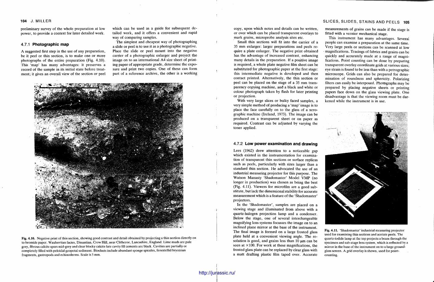
104 J .MILLER
preliminary survey of the whole preparat ion at low power , to provide a context for later detailed work.
4.7.1 Photographic map
A suggested first s tep in the use of any prepara t ion , be it peel or thin section, is to make one or more photographs of the entire preparat ion (Fig. 4.10). This 'map ' has many advantages: it preserves a record of the sample in its initial state before treatment ; it gives an overall view of the section or peel
which can be used as a guide for subsequent detailed work, and it offers a convenient and rapid way of comparing samples.
T h e simplest and cheapest way of photographing a slide or peel is to use it as a photographic negative. Place the slide or peel mount into the negative carrier of a photographic enlarger and project the image on to an international A 4 size sheet of printing paper of appropr ia te grade , de termine the exposure and print two copies. O n e of these can form part of a reference archive, the other is a working
Fig. 4.10. Negative print of thin section, showing good contrast and detail obtained by projecting a thin section directly on to bromide paper. Waulsortian facies, Dinantian, Crow Hill, near Clitheroe, Lancashire, England. Lime muds are pale grey, fibrous calcite spars mid-grey and clear blocky calcite late cavity fill cements are black. Cavities are partially or completely filled with peloidal geopetal sediment. Bioclasts include abundant sponge spicules, fenestellid bryozoan fragments, gastropods and echinoderms. Scale is 5 mm.
.1 iiimiiiiiiiimimiiHHMiHii
copy, upon which notes and details can be writ ten, or over which can be placed t ransparent overlays to mark grains, microprobe analysis sites etc.
Small thin sections will fit into the carrier of a 35 mm enlarger: larger preparat ions and peels require a plate enlarger. The negative print obtained has the advantage of increased contrast , enhancing many details in the preparat ion. If a positive image is required, a whole plate negative film sheet can be substituted for photographic paper at the first stage: this intermediate negative is developed and then contact pr inted. Alternatively, the thin section or peel can be placed on the stage of a 35 mm transparency copying machine, and a black and white or colour photograph taken by flash for later printing or projection.
With very large slices or bulky faced samples, a very simple method of producing a ' m a p ' image is to place the face carefully on to the glass of a xerographic machine (Ireland, 1973). The image can be produced on a t ransparent sheet or on paper as required. Contrast can be adjusted by varying the toner applied.
4.7.2 Low power examination and drawing
Lees (1962) drew at tention to a noticeable gap which existed in the instrumentat ion for examination of t ransparent thin sections or surface replicas such as peels, particularly with sizes larger than a s tandard thin section. H e advocated the use of an industrial measuring projector for this purpose. The Watson Manasty 'Shadomaster ' Model V M P (no longer in product ion) was chosen as being the best (Fig. 4.11). Viewers for microfilm are a good substitute, but lack the dimensional stability for accurate measurement which is a feature of the 'Shadomaster ' projectors.
In the 'Shadomaster ' , samples are placed on a viewing stage and illuminated from above with a quartz-halogen projection lamp and a condenser . Below the stage, one of several interchangeable magnifying lens systems focusses the image on to an inclined plane mirror at the base of the instrument. The final image is formed on a large frosted glass plate held at a convenient viewing angle. The resolution is good, and grains less than 10 u m can be seen at xlOO. For work at these magnifications, the frosted glass plate can be replaced by clear glass with a mat t drafting plastic film taped over. Accurate
SLICES, SLIDES, STAINS AND PEELS 105
Fig. 4.11. 'Shadomaster' industrial measuring projector used for examining thin sections and acetate peels. The quartz-iodide lamp at the top projects a beam through the specimen and sub-stage lens system, which is reflected by a mirror in the base of the instrument on to a large ground-glass screen. A grid overlay is shown, used for point-counting.
measurements of grains can be made if the stage is fitted with a vernier mechanical s tage.
This instrument has many advantages. Several people can examine a preparat ion at the same t ime. Very large peels or sections can be scanned at low
• magnifications. Tracings of fabrics and grains can be quickly and accurately m a d e at a range of magnifications. Point counting can be done by preparing t ransparent overlay coordinate grids at various sizes; eye strain is found to be less than with a petrographic microscope. Grids can also be prepared for determination of roundness and sphericity. Polarizing filters can easily be interposed. Photographs may be p repared by placing negative sheets or printing papers face down on the glass viewing plate. One disadvantage is that the viewing room must be darkened while the instrument is in use.
http://jurassic.ru/
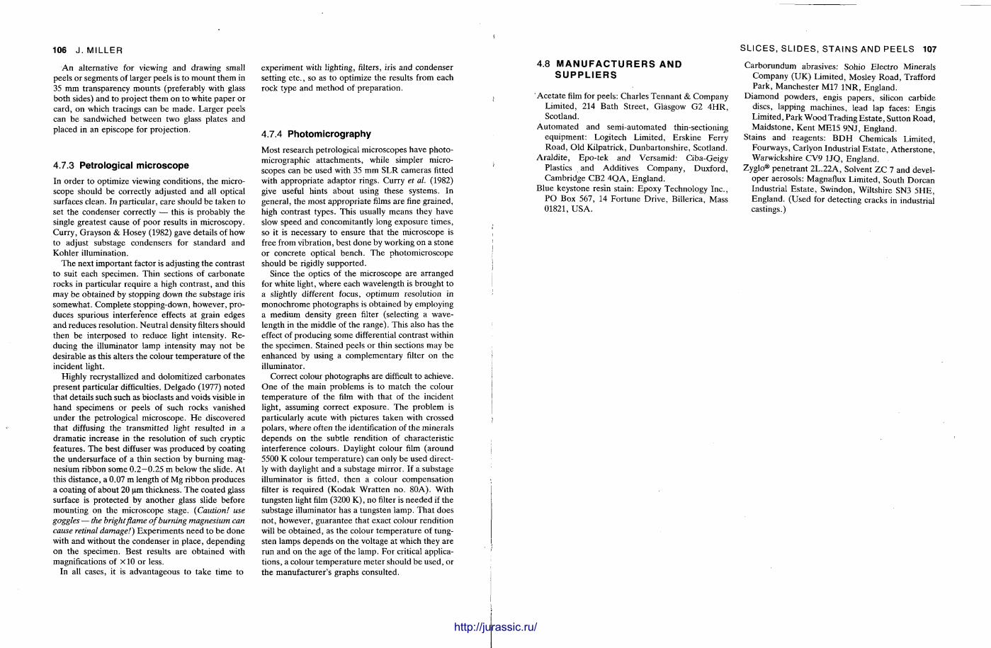
106 J . MILLER
A n alternative for viewing and drawing small peels or segments of larger peels is to moun t them in 35 mm transparency mounts (preferably with glass both sides) and to project them on to white paper or card, on which tracings can be made . Larger peels can be sandwiched between two glass plates and placed in an episcope for projection.
4.7.3 Petrological microscope
In order to optimize viewing conditions, the microscope should be correctly adjusted and all optical surfaces clean. In particular, care should be taken to set the condenser correctly — this is probably the single greatest cause of poor results in microscopy. Curry , Grayson & Hosey (1982) gave details of how to adjust substage condensers for s tandard and Kohler illumination.
The next important factor is adjusting the contrast to suit each specimen. Thin sections of carbonate rocks in particular require a high contrast , and this may be obtained by stopping down the substage iris somewhat . Comple te stopping-down, however , produces spurious interference effects at grain edges and reduces resolution. Neutral density filters should then be interposed to reduce light intensity. R e ducing the il luminator lamp intensity may not be desirable as this alters the colour t empera tu re of the incident light.
Highly recrystallized and dolomitized carbonates present particular difficulties. Delgado (1977) noted that details such such as bioclasts and voids visible in hand specimens or peels of such rocks vanished under the petrological microscope. H e discovered that diffusing the transmitted light resulted in a dramatic increase in the resolution of such cryptic features. T h e best diffuser was produced by coating the undersurface of a thin section by burning magnesium ribbon some 0.2—0.25 m below the slide. At this distance, a 0.07 m length of Mg ribbon produces a coating of about 20 urn thickness. The coated glass surface is protected by another glass slide before mount ing on the microscope stage. (Caution! use goggles — the bright flame of burning magnesium can cause retinal damage!) Exper iments need to be done with and without the condenser in place, depending on the specimen. Best results are obtained with magnifications of x l O or less.
In all cases, it is advantageous to take t ime to
experiment with lighting, filters, iris and condenser setting e tc . , so as to optimize the results from each rock type and method of preparat ion.
4.7.4 Photomicrography
Most research petrological microscopes have photo-micrographic a t tachments , while simpler microscopes can be used with 35 mm SLR cameras fitted with appropria te adaptor rings. Curry et al. (1982) give useful hints about using these systems. In genera] , the most appropr ia te films are fine grained, high contrast types. This usually means they have slow speed and concomitantly long exposure t imes, so it is necessary to ensure that the microscope is free from vibration, best done by working on a stone or concrete optical bench. The photomicroscope should be rigidly supported.
Since the optics of the microscope are arranged for white light, where each wavelength is brought to a slightly different focus, opt imum resolution in monochrome photographs is obtained by employing a medium density green filter (selecting a wavelength in the middle of the range) . This also has the effect of producing some differential contrast within the specimen. Stained peels or thin sections may be enhanced by using a complementary filter on the il luminator.
Correct colour photographs are difficult to achieve. O n e of the main problems is to match the colour t empera ture of the film with that of the incident light, assuming correct exposure. The problem is particularly acute with pictures taken with crossed polars, where often the identification of the minerals depends on the subtle rendition of characteristic interference colours. Daylight colour film (around 5500 K colour tempera ture) can only be used directly with daylight and a substage mirror. If a substage il luminator is fitted, then a colour compensat ion filter is required (Kodak Wrat ten no. 80A) . With tungsten light film (3200 K ) , no filter is needed if the substage il luminator has a tungsten lamp. Tha t does not , however , guarantee that exact colour rendition will be obtained, as the colour t empera ture of tungsten lamps depends on the voltage at which they are run and on the age of the lamp. For critical applicat ions, a colour t empera ture meter should be used, or the manufacturer 's graphs consulted.
l l i l i i
4.8 M A N U F A C T U R E R S A N D S U P P L I E R S
Aceta te film for peels: Charles Tennan t & Company Limited, 214 Bath Street , Glasgow G2 4 H R , Scotland.
Automated and semi-automated thin-sectioning equipment : Logitech Limited, Erskine Ferry Road , Old Kilpatrick, Dunbar tonshi re , Scotland.
Araldi te , Epo- tek and Versamid: Ciba-Geigy Plastics and Additives Company, Duxford, Cambridge CB2 4 Q A , England.
Blue keystone resin stain: Epoxy Technology Inc . , P O Box 567, 14 For tune Drive, Billerica, Mass 01821, U S A .
SLICES, SLIDES, STAINS AND PEELS 107
Carborundum abrasives: Sohio Electro Minerals Company ( U K ) Limited, Mosley Road , Trafford Park, Manchester M17 1NR, England.
D iamond powders , engis papers , silicon carbide discs, lapping machines, lead lap faces: Engis Limited, Park Wood Trading Es ta te , Sutton Road , Maids tone , Ken t M E 1 5 9NJ , England.
Stains and reagents: B D H Chemicals Limited, Fourways , Carlyon Industrial Es ta te , Athers tone , Warwickshire CV9 1JQ, England.
Zyglo® penet rant 2L.22A, Solvent Z C 7 and developer aerosols: Magnaflux Limited, South Dorcan Industrial Es ta te , Swindon, Wiltshire SN3 5 H E , England. (Used for detecting cracks in industrial castings.)
http://jurassic.ru/
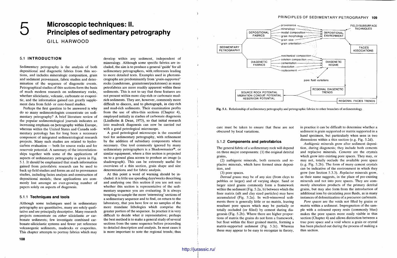
5 PRINCIPLES OF SEDIMENTARY PETROGRAPHY 109
Microscopic techniques: II. Principles of sedimentary petrography GILL HARWOOD
5.1 I N T R O D U C T I O N
Sedimentary petrography is the analysis of both depositional and diagenetic fabrics from thin sect ions, and includes mineralogic composit ion, grain and sediment provenance , fabric studies and determination of the sequence of diagenetic events . Petrographical studies of thin sections form the basis of much modern research on sedimentary rocks, whether siliciclastic, volcanic, carbonate or evapori-tic, and the information gained can greatly supplement data from field- or core-based studies.
Perhaps the first quest ion to be answered is why do so many sedimentologists concentra te on sedimentary petrography? A brief l i terature review of the popular sedimentological journals indicates an increasing emphasis on pet rography within E u r o p e , whereas within the Uni ted States and Canada sedimentary petrology has for long been a necessary component of integrated sedimentological research projects. Many such studies are related to hydrocarbon evaluation — both for source rocks and for reservoir potent ial . A summary of the interrelat ionships together with some of the applications of aspects of sedimentary petrography is given in Fig. 5 .1 . It should be emphasized that much information gained from petrofabric research can be used to back up field studies and forms an aid to provenance studies, including facies analysis and construction of depositional models ; these applications are commonly lost amongst an ever-growing number of papers solely on aspects of diagenesis.
5.1.1 Techniques and tools
Although some techniques used in sedimentary petrography are quanti tat ive, many are solely qualitative and are principally descriptive. Many research projects concentrate on either siliciclastic or carbonate sediments; few investigate combined car-bonate-siliciclastic systems and fewer yet reference volcanogenic sediments , mudrocks or evapori tes . This chapter a t tempts to portray fabrics which may
develop within any sediment , independent of mineralogy. Al though some specific fabrics are included, the aim is to produce a general 'guide ' for all sedimentary pet rographers , with references leading to more detailed texts. Examples used in photomicrographs are predominant ly from 'grain-supported'' rocks (sandstones, grainstones/packstones) as many petrofabrics are more readily apparent within these sediments . This is not to say that these features are not present within more clay-rich or carbonate mud-rich sediments . They a re , however , commonly more difficult to discern, and to photograph , in clay-rich and mud-rich sediments . Their examination profits from the use of ultra-thin sections (Chapter 4) , employed initially in studies of carbonate diagenesis (Lindholm & D e a n , 1973), so that initial research into mudrock diagenesis can now be carried out with a good petrological microscope.
A good petrological microscope is the essential tool for sedimentary pet rography, with refinement by the addition of subsidiary components where necessary. O n e tool commonly ignored by many sedimentary pet rographers is a Shadowmaster®, or similar equipment , where a thin section is projected on to a ground glass screen to produce an image (a shadowgraph) . This can be extremely useful for overviews of a thin section, grain shape and size determinat ions and for fabric analysis.
A t this point a word of warning should be included: it is little use spending days/weeks describing and analysing one thin section if you are not sure whether this section is representat ive of the sedimentary sequence you are evaluating. It is always tempting to sample the more ' interesting' sections of a sedimentary sequence and to find, on re turn to the laboratory, that you have few or no samples of the more mundane lithologies which comprise the greater port ion of the sequence. In practice it is very difficult to decide what is representat ive; perhaps the best method is to m a k e a general study of several sections from the same sequence before proceeding to detailed description and analysis. In most cases it is more important to note the regional t rends; thus
DEPOSITIONAL FABRICS
SEDIMENTARY PETROGRAPHY
DIAGENETIC FABRICS
provenance minera logy modal compos i t i on grain morphology grain size grain orientation
-mechan ica l compac t ion -solut ion compac t ion -cementa t ion -d issolut ion — - rep lacement
FIELD/SUBSURFACE TECHNIQUES
SOURCE ROCK POTENTIAL MIGRATION CONDUIT POTENTIAL
RESERVOIR POTENTIAL
Fig. 5 . 1 . Relationship of sedimentary petrography and petrographic fabrics to other branches of sedimentology.
care must be taken to ensure that these are not obscured by local variations.
5.1.2 Components and petrofabrics
The general fabric of a sedimentary rock will depend on three major components : (1) the original detrital grains,
(2) authigenic minerals , both cements and re-placive minerals , which have formed since deposition, and
(3) pore spaces. Detrital grains may be of any size (from clays to
pebbles or larger) and of varying shape. Sand or larger sized grains commonly form a framework within the sediment (Fig. 5.2a, b) between which the finer matrix (silt and clay sized particles) may have accumulated (Fig. 5.2a). In well-winnowed sediments there is generally little or no matrix, leaving resultant pore spaces which may be partially or totally occluded (or filled) by cement during diagenesis (Fig. 5.2b). Where there are higher proportions of matrix the grains do not form a framework, but float within the finer grained matrix, forming a matrix-supported sediment (Fig. 5.2c). Whereas these may appear to be easy to recognize in theory,
in practice it can be difficult to determine whether a sediment is grain supported or matrix supported in a hand specimen, but particularly when seen in two dimensions within a thin section (e.g. Fig. 5.2d).
Authigenic minerals grow after sediment deposition, during diagenesis; they include both cements and replacive minerals. Cements are the crystals which grow into existing pore spaces. They may, or may not , totally occlude the available pore space (e.g. Fig. 5.2b). The form of many cement crystals can be indicative of the environment in which they grew (see Section 5.3.3). Replacive minerals grow, as their n a m e suggests, in the place of pre-existing minerals and not into pore spaces. They are commonly alteration products of the primary detrital grains, but may also form from the introduction of additional ions by circulating pore fluids, as in many instances of dolomitization of a precursor carbonate .
Pore spaces are the voids not filled by grains or matrix within a sediment. Impregnation of the sample with a coloured epoxy resin (commonly blue) makes the pore spaces more easily visible in thin section (Chapter 4) and allows distinction between a t rue pore space and a void where a grain or crystal has been plucked out during the process of making a thin section.
llllllllllllllllllllHMIIIIIIIIIIIIIIIIIIIIllllllf
108
http://jurassic.ru/
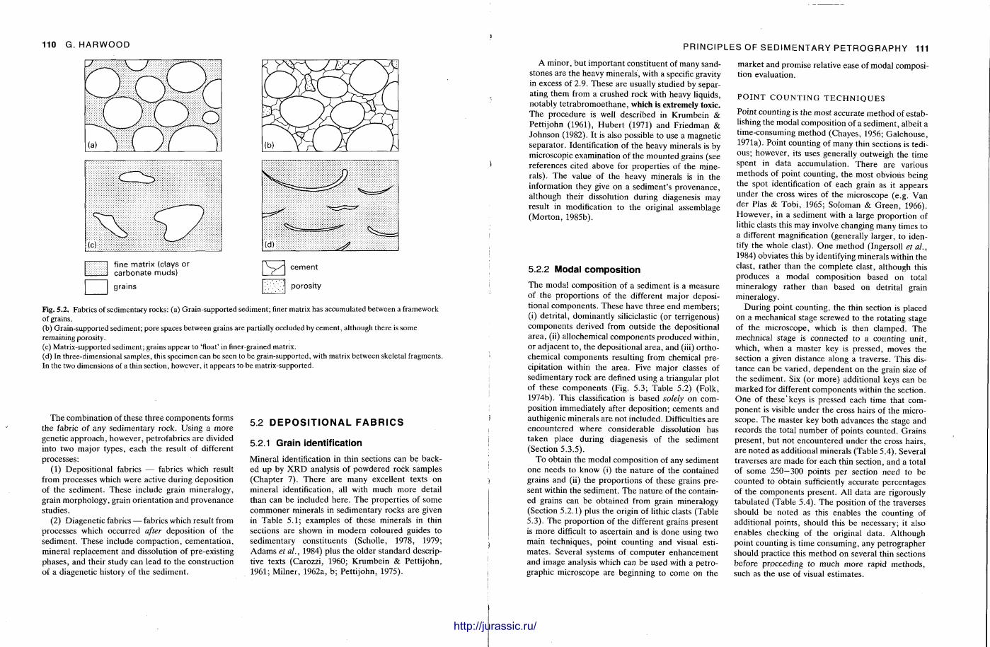
110 G. HARWOOD
fine matrix (clays or carbonate muds)
grains
cemen t
porosity
Fig. 5.2. Fabrics of sedimentary rocks: (a) Grain-supported sediment; finer matrix has accumulated between a framework of grains. (b) Grain-supported sediment; pore spaces between grains are partially occluded by cement, although there is some remaining porosity. (c) Matrix-supported sediment; grains appear to 'float' in finer-grained matrix. (d) In three-dimensional samples, this specimen can be seen to be grain-supported, with matrix between skeletal fragments. In the two dimensions of a thin section, however, it appears to be matrix-supported.
The combination of these three components forms the fabric of any sedimentary rock. Using a more genetic approach, however , petrofabrics are divided into two major types, each the result of different processes:
(1) Deposit ional fabrics — fabrics which result from processes which were active during deposition of the sediment. These include grain mineralogy, grain morphology, grain orientation and provenance studies.
(2) Diagenetic fabrics — fabrics which result from processes which occurred after deposition of the sediment. These include compact ion, cementat ion, mineral replacement and dissolution of pre-existing phases, and their study can lead to the construction of a diagenetic history of the sediment.
5.2 D E P O S I T I O N A L F A B R I C S
5.2.1 Grain identif ication
Mineral identification in thin sections can be backed up by X R D analysis of powdered rock samples (Chapter 7) . The re are many excellent texts on mineral identification, all with much more detail than can be included here . The propert ies of some commoner minerals in sedimentary rocks are given in Table 5 .1 ; examples of these minerals in thin sections are shown in modern coloured guides to sedimentary consti tuents (Scholle, 1978, 1979; Adams et al., 1984) plus the older s tandard descriptive texts (Carozzi, 1960; Krumbein & Pett i john, 1961; Milner, 1962a, b ; Pett i john, 1975).
PRINCIPLES OF SEDIMENTARY PETROGRAPHY 111
A minor, but important constituent of many sandstones are the heavy minerals , with a specific gravity in excess of 2.9. These are usually studied by separating them from a crushed rock with heavy liquids, notably t e t rabromoethane , which is extremely toxic. The procedure is well described in Krumbein & Pett i john (1961), Hube r t (1971) and Fr iedman & Johnson (1982). It is also possible to use a magnetic separator . Identification of the heavy minerals is by microscopic examination of the mounted grains (see references cited above for propert ies of the minerals). The value of the heavy minerals is in the information they give on a sediment 's provenance, al though their dissolution during diagenesis may result in modification to the original assemblage (Mor ton , 1985b).
5.2.2 Modal composi t ion
The modal composition of a sediment is a measure of the proport ions of the different major depositional components . These have three end members ; (i) detri tal , dominantly siliciclastic (or terrigenous) components derived from outside the depositional area , (ii) allochemical components produced within, or adjacent to , the depositional area , and (iii) or tho-chemical components resulting from chemical precipitation within the area. Five major classes of sedimentary rock are defined using a triangular plot of these components (Fig. 5.3; Table 5.2) (Folk, 1974b). This classification is based solely on composition immediately after deposit ion; cements and authigenic minerals are not included. Difficulties are encountered where considerable dissolution has taken place during diagenesis of the sediment (Section 5.3.5).
To obtain the modal composition of any sediment one needs t o know (i) the na ture of the contained grains and (ii) the proport ions of these grains present within the sediment. The nature of the contained grains can be obta ined from grain mineralogy (Section 5.2.1) plus the origin of lithic clasts (Table 5.3). The propor t ion of the different grains present is more difficult to ascertain and is done using two main techniques, point counting and visual estimates . Several systems of computer enhancement and image analysis which can be used with a petrographic microscope are beginning to come on the
marke t and promise relative ease of modal composition evaluation.
P O I N T C O U N T I N G T E C H N I Q U E S
Point counting is the most accurate method of establishing the modal composition of a sediment, albeit a t ime-consuming method (Chayes, 1956; Gatehouse , 1971a). Point counting of many thin sections is tedious; however, its uses generally outweigh the time spent in data accumulation. The re are various methods of point counting, the most obvious being the spot identification of each grain as it appears under the cross wires of the microscope (e.g. Van der Plas & Tobi , 1965; Soloman & Green , 1966). However , in a sediment with a large proport ion of lithic clasts this may involve changing many times t o a different magnification (generally larger, to identify the whole clast). O n e method (Ingersoll et al., 1984) obviates this by identifying minerals within the clast, ra ther than the complete clast, although this produces a modal composit ion based on total mineralogy rather than based on detrital grain mineralogy.
Dur ing point counting, the thin section is placed on a mechanical stage screwed to the rotating stage of the microscope, which is then clamped. The mechnical stage is connected to a counting unit, which, when a master key is pressed, moves the section a given distance along a t raverse. This distance can be varied, dependent on the grain size of the sediment. Six (or more) additional keys can be marked for different components within the section. One of these 'keys is pressed each time that componen t is visible under the cross hairs of the microscope. The master key both advances the stage and records the total number of points counted. Grains present , but not encountered under the cross hairs, are noted as additional minerals (Table 5.4). Several traverses are made for each thin section, and a total of some 250—300 points per section need to be counted to obtain sufficiently accurate percentages of the components present . All data are rigorously tabulated (Table 5.4). The position of the traverses should be noted as this enables the counting of additional points, should this be necessary; it also enables checking of the original data. Al though point counting is t ime consuming, any petrographer should practice this method on several thin sections before proceeding to much more rapid methods , such as the use of visual est imates.
http://jurassic.ru/
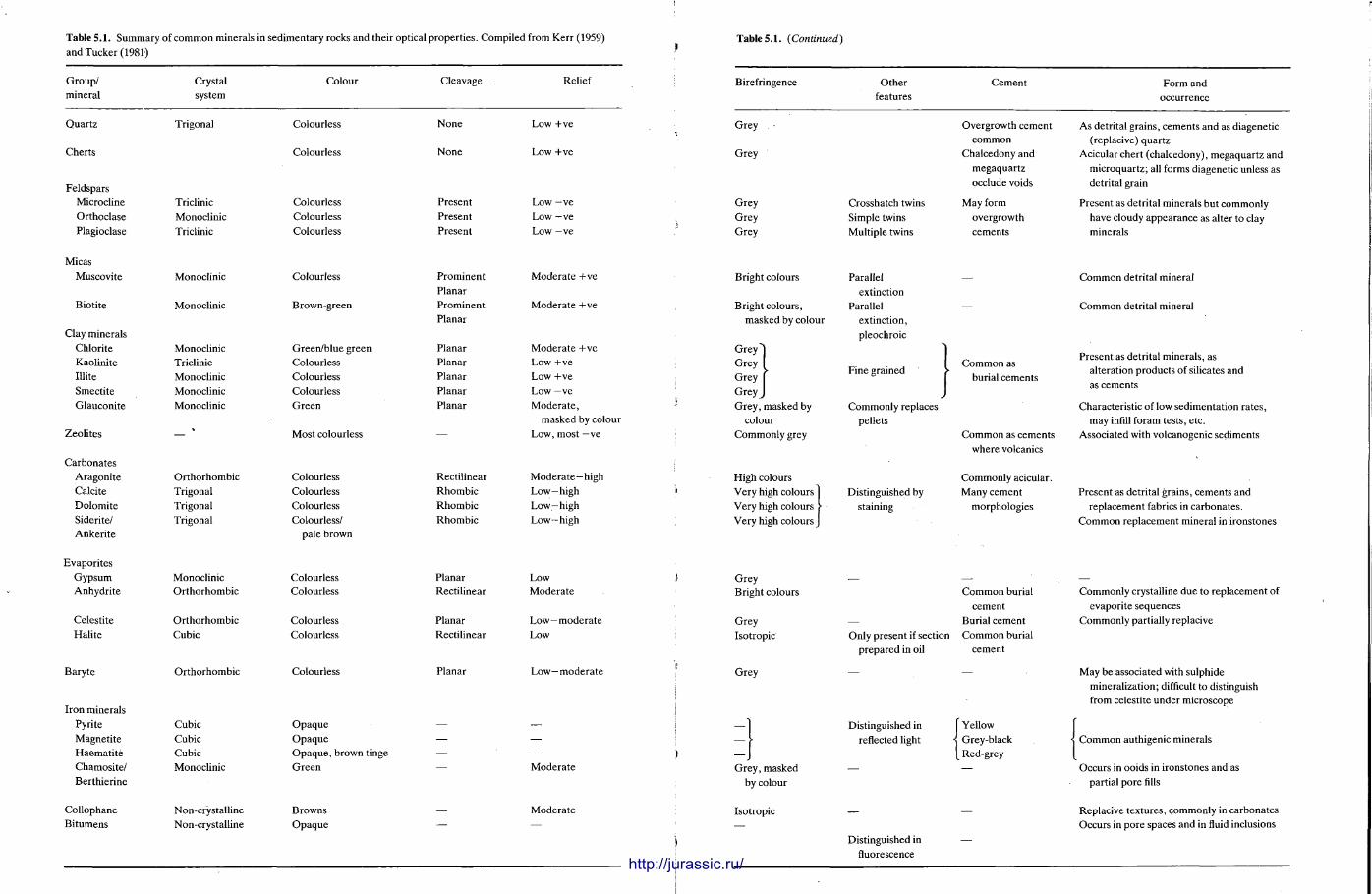
Table 5 . 1 . S U M M A R Y O F C O M M O N M I N E R A L S I N S E D I M E N T A R Y R O C K S A N D T H E I R O P T I C A L P R O P E R T I E S . C O M P I L E D F R O M K E R R ( 1 9 5 9 )
A N D T U C K E R ( 1 9 8 1 )
G R O U P /
M I N E R A L
C R Y S T A L
S Y S T E M
C O L O U R C L E A V A G E R E L I E F
Quartz
Cherts
T R I G O N A L C O L O U R L E S S
C O L O U R L E S S
N O N E
N O N E
L O W + V E
L O W + V E
F E L D S P A R S
M I C R O C L I N E
O R T H O C L A S E
P L A G I O C L A S E
T R I C L I N I C
M O N O C L I N I C
T R I C L I N I C
C O L O U R L E S S
C O L O U R L E S S
C O L O U R L E S S
P R E S E N T
P R E S E N T
P R E S E N T
L O W — V E
L O W - V E
L O W — V E
M I C A S
M U S C O V I T E
B I O T I T E
C L A Y M I N E R A L S
C H L O R I T E
K A O L I N I T E
I L L I T E
S M E C T I T E
G L A U C O N I T E
Z E O L I T E S
M O N O C L I N I C
M O N O C L I N I C
M O N O C L I N I C
T R I C L I N I C
M O N O C L I N I C
M O N O C L I N I C
M O N O C L I N I C
C O L O U R L E S S
B R O W N - G R E E N
G R E E N / B L U E G R E E N
C O L O U R L E S S
C O L O U R L E S S
C O L O U R L E S S
G R E E N
M O S T C O L O U R L E S S
P R O M I N E N T
P L A N A R
P R O M I N E N T
P L A N A R
P L A N A R
P L A N A R
P L A N A R
P L A N A R
P L A N A R
M O D E R A T E + V E
M O D E R A T E + V E
M O D E R A T E + V E
L O W + V E
L O W + V E
L O W — V E
M O D E R A T E ,
M A S K E D B Y C O L O U R
L O W , M O S T — V E
C A R B O N A T E S
A R A G O N I T E
C A L C I T E
D O L O M I T E
S I D E R I T E /
A N K E R I T E
E V A P O R I T E S
G Y P S U M
A N H Y D R I T E
C E L E S T I T E
H A L I T E
O R T H O R H O M B I C
T R I G O N A L
T R I G O N A L
T R I G O N A L
M O N O C L I N I C
O R T H O R H O M B I C
O R T H O R H O M B I C
C U B I C
C O L O U R L E S S
C O L O U R L E S S
C O L O U R L E S S
C O L O U R L E S S /
P A L E B R O W N
C O L O U R L E S S
C O L O U R L E S S
C O L O U R L E S S
C O L O U R L E S S
R E C T I L I N E A R
R H O M B I C
R H O M B I C
R H O M B I C
P L A N A R
R E C T I L I N E A R
P L A N A R
R E C T I L I N E A R
M O D E R A T E — H I G H
L O W — H I G H
L O W — H I G H
L O W - H I G H
L O W
M O D E R A T E
L O W — M O D E R A T E
L O W
B A R Y T E O R T H O R H O M B I C C O L O U R L E S S P L A N A R L O W — M O D E R A T E
I R O N M I N E R A L S
P Y R I T E
M A G N E T I T E
H A E M A T I T E
C H A M O S I T E /
B E R T H I E R I N E
C U B I C
C U B I C
C U B I C
M O N O C L I N I C
O P A Q U E
O P A Q U E
O P A Q U E , B R O W N T I N G E
G R E E N M O D E R A T E
C O L L O P H A N E
B I T U M E N S
N O N - C R Y S T A L L I N E
N O N - C R Y S T A L L I N E
B R O W N S
O P A Q U E
M O D E R A T E
Table 5 . 1 . (Continued)
B I R E F R I N G E N C E O T H E R
F E A T U R E S
C E M E N T F O R M A N D
O C C U R R E N C E
G R E Y
G R E Y
G R E Y
G R E Y
G R E Y
C R O S S H A T C H T W I N S
S I M P L E T W I N S
M U L T I P L E T W I N S
O V E R G R O W T H C E M E N T
C O M M O N
C H A L C E D O N Y A N D
M E G A Q U A R T Z
O C C L U D E V O I D S
M A Y F O R M
O V E R G R O W T H
C E M E N T S
A S D E T R I T A L G R A I N S , C E M E N T S A N D A S D I A G E N E T I C
( R E P L A C I V E ) Q U A R T Z
A C I C U L A R C H E R T ( C H A L C E D O N Y ) , M E G A Q U A R T Z A N D
M I C R O Q U A R T Z ; ALL F O R M S D I A G E N E T I C U N L E S S A S
D E T R I T A L G R A I N
P R E S E N T A S D E T R I T A L M I N E R A L S B U T C O M M O N L Y
H A V E C L O U D Y A P P E A R A N C E A S A L T E R T O C L A Y
M I N E R A L S
B R I G H T C O L O U R S
B R I G H T C O L O U R S ,
M A S K E D B Y C O L O U R
G R E Y
G R E Y
G R E Y
G R E Y ^
G R E Y , M A S K E D B Y
C O L O U R
C O M M O N L Y G R E Y
P A R A L L E L
E X T I N C T I O N
P A R A L L E L
E X T I N C T I O N ,
P L E O C H R O I C
F I N E G R A I N E D
C O M M O N L Y R E P L A C E S
P E L L E T S
C O M M O N A S
B U R I A L C E M E N T S
C O M M O N A S C E M E N T S
W H E R E V O L C A N I C S
C O M M O N D E T R I T A L M I N E R A L
C O M M O N D E T R I T A L M I N E R A L
P R E S E N T A S D E T R I T A L M I N E R A L S , A S
A L T E R A T I O N P R O D U C T S O F S I L I C A T E S A N D
A S C E M E N T S
C H A R A C T E R I S T I C O F L O W S E D I M E N T A T I O N R A T E S ,
M A Y INF ILL F O R A M T E S T S , E T C .
A S S O C I A T E D W I T H V O L C A N O G E N I C S E D I M E N T S
H I G H C O L O U R S
V E R Y H I G H C O L O U R S |
V E R Y H I G H C O L O U R S >
V E R Y H I G H C O L O U R S J
D I S T I N G U I S H E D B Y
S T A I N I N G
C O M M O N L Y A C I C U L A R .
M A N Y C E M E N T
M O R P H O L O G I E S
P R E S E N T A S D E T R I T A L G R A I N S , C E M E N T S A N D
R E P L A C E M E N T F A B R I C S I N C A R B O N A T E S .
C O M M O N R E P L A C E M E N T M I N E R A L I N I R O N S T O N E S
G R E Y
B R I G H T C O L O U R S
G R E Y
I S O T R O P I C
G R E Y
G R E Y , M A S K E D
B Y C O L O U R
I S O T R O P I C
C O M M O N B U R I A L
C E M E N T
— B U R I A L C E M E N T
O N L Y P R E S E N T I F S E C T I O N C O M M O N B U R I A L
P R E P A R E D I N O I L C E M E N T
D I S T I N G U I S H E D I N
R E F L E C T E D L I G H T
( " Y E L L O W
-{ G R E Y - B L A C K
[ R E D - G R E Y
D I S T I N G U I S H E D I N
FLUORESCENCE
C O M M O N L Y C R Y S T A L L I N E D U E T O R E P L A C E M E N T O F
E V A P O R I T E S E Q U E N C E S
C O M M O N L Y P A R T I A L L Y R E P L A C I V E
M A Y B E A S S O C I A T E D W I T H S U L P H I D E
M I N E R A L I Z A T I O N ; D I F F I C U L T T O D I S T I N G U I S H
F R O M C E L E S T I T E U N D E R M I C R O S C O P E
C O M M O N A U T H I G E N I C M I N E R A L S
O C C U R S I N O O I D S I N I R O N S T O N E S A N D A S
P A R T I A L P O R E FILLS
R E P L A C I V E T E X T U R E S , C O M M O N L Y I N C A R B O N A T E S
O C C U R S I N P O R E S P A C E S A N D I N FLUID I N C L U S I O N S
http://jurassic.ru/
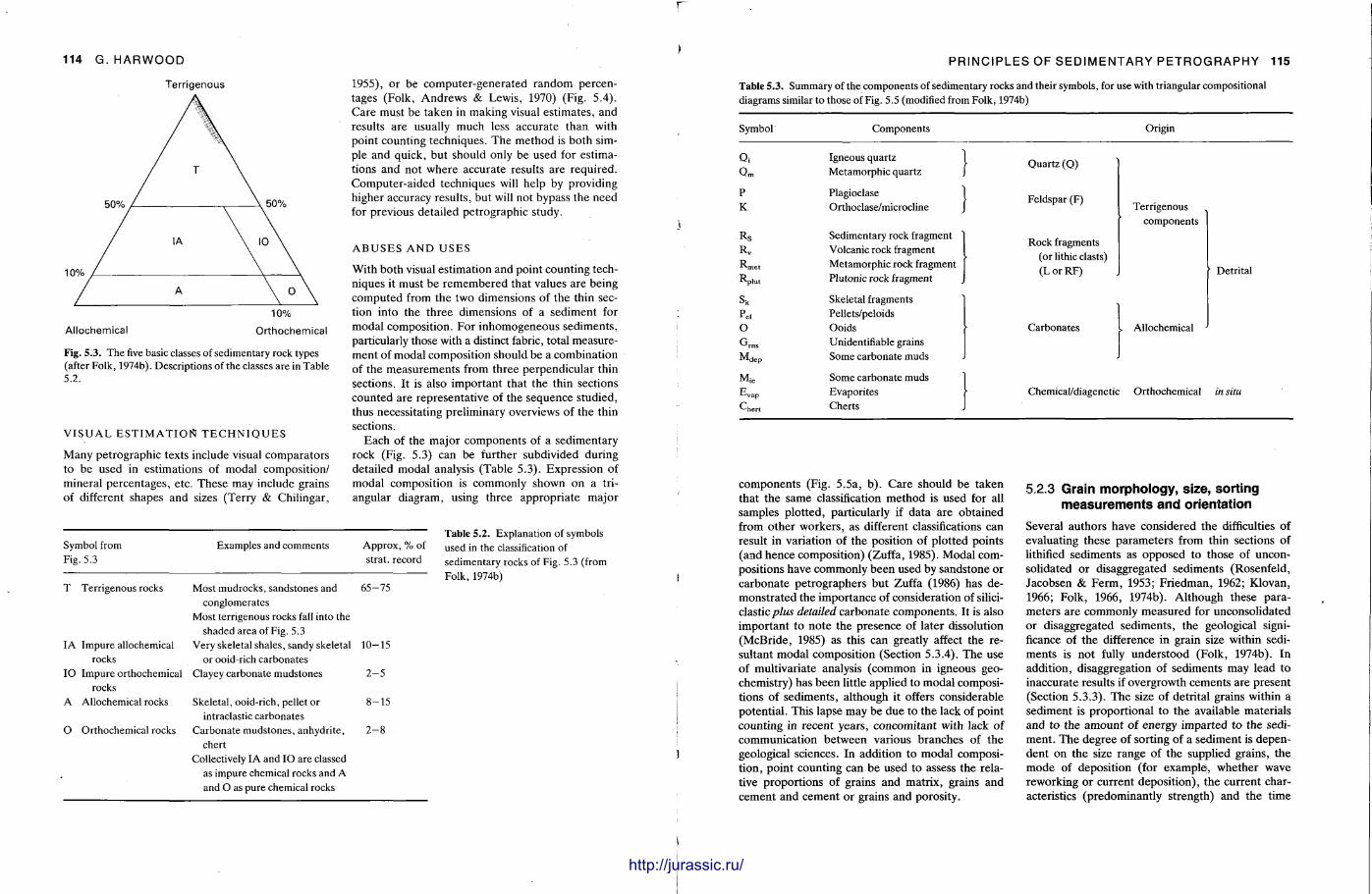
114 G. HARWOOD
10% Allochemical Orthochemical
Fig. 5.3. The five basic classes of sedimentary rock types (after Folk, 1974b). Descriptions of the classes are in Table 5.2.
V I S U A L E S T I M A T I O N T E C H N I Q U E S
Many petrographic texts include visual comparators to be used in estimations of modal composition/ mineral percentages, etc. These may include grains of different shapes and sizes (Terry & Chilingar,
1955), or be computer-generated random percentages (Folk, Andrews & Lewis, 1970) (Fig. 5.4). Care must be taken in making visual est imates, and results are usually much less accurate than with point counting techniques. The method is both simple and quick, but should only be used for estimations and not where accurate results are required. Computer-aided techniques will help by providing higher accuracy results, but will not bypass the need for previous detailed petrographic study.
A B U S E S A N D U S E S
With both visual estimation and point counting techniques it must be remembered that values are being computed from the two dimensions of the thin section into the three dimensions of a sediment for modal composit ion. For inhomogeneous sediments , particularly those with a distinct fabric, total measurement of modal composition should be a combinat ion of the measurements from three perpendicular thin sections. It is also important that the thin sections counted are representat ive of the sequence studied, thus necessitating preliminary overviews of the thin sections.
Each of the major components of a sedimentary rock (Fig. 5.3) can be further subdivided during detailed modal analysis (Table 5.3). Expression of modal composition is commonly shown on a triangular diagram, using three appropria te major
Symbol from Fig. 5.3
Examples and comments Approx, % of strat. record
T Terrigenous rocks Most mudrocks, sandstones and 65- 75 conglomerates
Most terrigenous rocks fall into the shaded area of Fig. 5.3
IA Impure allochemical Very skeletal shales, sandy skeletal 10- 15 rocks or ooid-rich carbonates
IO Impure orthochemical Clayey carbonate mudstones 2 - 5 rocks
A Allochemical rocks Skeletal, ooid-rich, pellet or 8- 15 intraclastic carbonates
O Orthochemical rocks Carbonate mudstones, anhydrite, 2 - 8 chert
Collectively IA and IO are classed as impure chemical rocks and A and O as pure chemical rocks
Table 5.2. Explanation of symbols used in the classification of sedimentary rocks of Fig. 5.3 (from Folk, 1974b)
llllllllillillililiilllllll
PRINCIPLES OF SEDIMENTARY PETROGRAPHY 115
Symbol Components Origin
Qi Igneous quartz Q m
Metamorphic quartz J P Plagioclase ] K
Orthoclase/microcline J
Rs Sedimentary rock fragment
Rv Volcanic rock fragment
Rmet Metamorphic rock fragment
Rpiut Plutonic rock fragment
Skeletal fragments
Pel Pellets/peloids O Ooids G r n s
Unidentifiable grains M d e p
Some carbonate muds
M i c Some carbonate muds F
v̂ap Evaporites
Chert Cherts
Quartz (Q)
Feldspar (F)
Rock fragments (or lithic clasts) (LorRF)
Carbonates
Terrigenous components
Allochemical
Detrital
Chemical/diagenetic Orthochemical in situ
components (Fig. 5.5a, b ) . Care should be taken that the same classification method is used for all samples plot ted, particularly if data are obtained from other workers , as different classifications can result in variation of the position of plotted points (and hence composit ion) (Zuffa, 1985). Modal compositions have commonly been used by sandstone or carbonate pet rographers but Zuffa (1986) has demonst ra ted the importance of consideration of siliciclastic plus detailed carbonate components . It is also important to note the presence of later dissolution (McBride, 1985) as this can greatly affect the resultant modal composit ion (Section 5.3.4). The use of multivariate analysis (common in igneous geochemistry) has been little applied to modal compositions of sediments , al though it offers considerable potent ial . This lapse may be due to the lack of point counting in recent years, concomitant with lack of communicat ion between various branches of the geological sciences. In addition to modal composit ion, point counting can be used to assess the relative proport ions of grains and matrix, grains and cement and cement or grains and porosity.
5,2.3 Grain morphology, size, sort ing measurements and orientation
Several authors have considered the difficulties of evaluating these parameters from thin sections of lithified sediments as opposed to those of unconsolidated or disaggregated sediments (Rosenfeld, Jacobsen & Fe rm, 1953; Fr iedman, 1962; Klovan, 1966; Folk, 1966, 1974b). Al though these parameters are commonly measured for unconsolidated or disaggregated sediments , the geological significance of the difference in grain size within sediments is not fully unders tood (Folk, 1974b). In addit ion, disaggregation of sediments may lead to inaccurate results if overgrowth cements are present (Section 5.3.3). The size of detrital grains within a sediment is proport ional to the available materials and to the amoun t of energy imparted to the sediment . The degree of sorting of a sediment is dependent on the size range of the supplied grains, the m o d e of deposition (for example, whether wave reworking or current deposi t ion) , the current characteristics (predominantly strength) and the time
1111
Terrigenous Table 5.3. Summary of the components of sedimentary rocks and their symbols, for use with triangular compositional diagrams similar to those of Fig. 5.5 (modified from Folk, 1974b)
http://jurassic.ru/
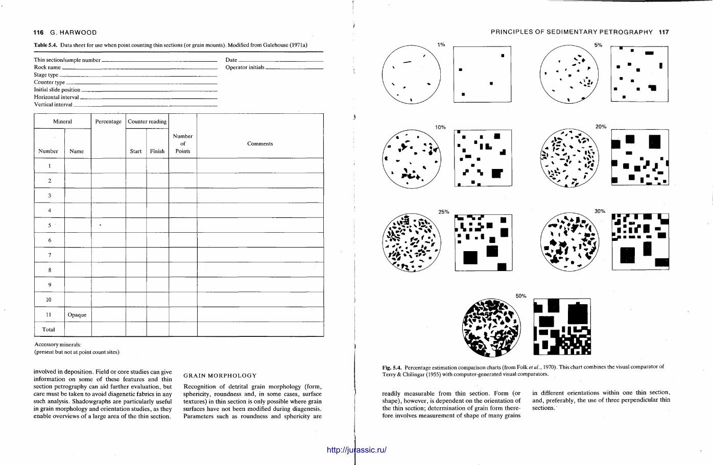
r i
) 116 G. HARWOOD
Table 5 . 4 . Data sheet for use when point counting thin sections (or grain mounts). Modified from Galehouse (1971a)
Thin section/sample number Date Rock name : Operator initials : • Stage type :
Counter type : : Initial slide position . Horizontal interval Vertical interval
Mineral Percentage Counter reading
Number of
Points Comments
Number Name
Percentage
Start Finish
Number of
Points Comments
1
2
3
4
5 ' •
6
7
8
9
10
11 Opaque
Total
Accessory minerals: (present but not at point count sites)
involved in deposit ion. Field or core studies can give information on some of these features and thin section petrography can aid further evaluation, but care must be taken to avoid diagenetic fabrics in any such analysis. Shadowgraphs are particularly useful in grain morphology and orientation studies, as they enable overviews of a large area of the thin section.
G R A I N M O R P H O L O G Y
Recognition of detrital grain morphology (form, sphericity, roundness and, in some cases, surface textures) in thin section is only possible where grain surfaces have not been modified during diagenesis. Parameters such as roundness and sphericity are
PRINCIPLES OF SEDIMENTARY PETROGRAPHY 117
Fig. 5 . 4 . Percentage estimation comparison charts (from Folk et al., 1970). This chart combines the visual comparator of Terry & Chilingar (1955) with computer-generated visual comparators.
readily measurable from thin section. Form (or in different orientat ions within one thin section, shape) , however , is dependent on the orientation of and, preferably, the use of three perpendicular thin the thin section; determinat ion of grain form there- sections, fore involves measurement of shape of many grains
http://jurassic.ru/
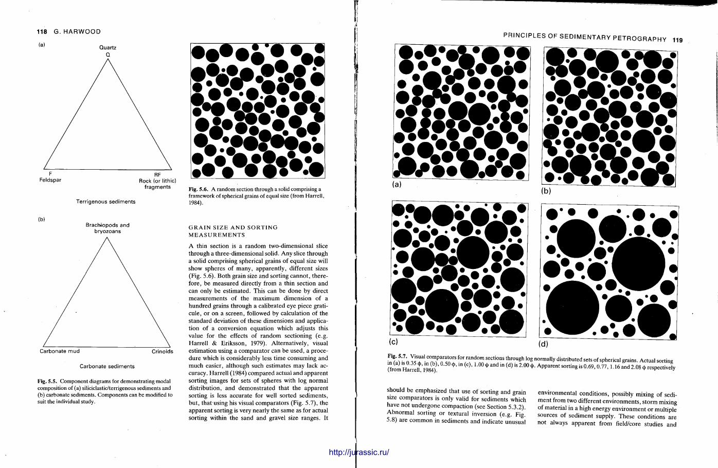
118 G. HARWOOD
Quartz Q
F RF Feldspar Rock (or lithic)
fragments
Terrigenous sediments
(b) Brachiopods and
bryozoans
Carbonate mud Crinoids
Carbonate sediments
Fig. 5 . 5 . Component diagrams for demonstrating modal composition of (a) siliciclastic/terrigenous sediments and (b) carbonate sediments. Components can be modified to suit the individual study.
Fig. 5 .6 . A random section through a solid comprising a framework of spherical grains of equal size (from Harrell, 1984).
G R A I N S I Z E A N D S O R T I N G M E A S U R E M E N T S
A thin section is a random two-dimensional slice through a three-dimensional solid. Any slice through a solid comprising spherical grains of equal size will show spheres of many, apparent ly, different sizes (Fig. 5.6). Both grain size and sorting cannot , therefore, be measured directly from a thin section and can only be est imated. This can be done by direct measurements of the maximum dimension of a hundred grains through a calibrated eye piece graticule, or on a screen, followed by calculation of the s tandard deviation of these dimensions and application of a conversion equat ion which adjusts this value for the effects of random sectioning (e.g. Harrel l & Eriksson, 1979). Alternatively, visual estimation using a compara tor can be used, a procedure which is considerably less t ime consuming and much easier, al though such estimates may lack accuracy. Harrel l (1984) compared actual and apparent sorting images for sets of spheres with log normal distribution, and demonst ra ted that the apparent sorting is less accurate for well sorted sediments , but , that using his visual comparators (Fig. 5.7), the apparent sorting is very nearly the same as for actual sorting within the sand and gravel size ranges. It
PRINCIPLES OF SEDIMENTARY PETROGRAPHY 119
( 0 (d)
Fig. 5 .7 . Visual comparators for random sections through log normally distributed sets of spherical grains. Actual sorting in (a) is 0.35 <t>, in (b), 0.50 <t>, in (c), 1.00 (j> and in (d) is 2.00 <t>. Apparent sorting is 0.69,0.77,1.16 and 2.08 (j) respectively (from Harrell, 1984).
should be emphasized that use of sorting and grain environmental conditions, possibly mixing of sedi-size comparators is only valid for sediments which ment from two different envi ronments , s torm mixing have not undergone compaction (see Section 5.3.2). of material in a high energy environment or multiple Abnormal sorting or textural inversion (e.g. Fig. sources of sediment supply. These conditions are 5.8) are common in sediments and indicate unusual not always apparent from field/core studies and
http://jurassic.ru/
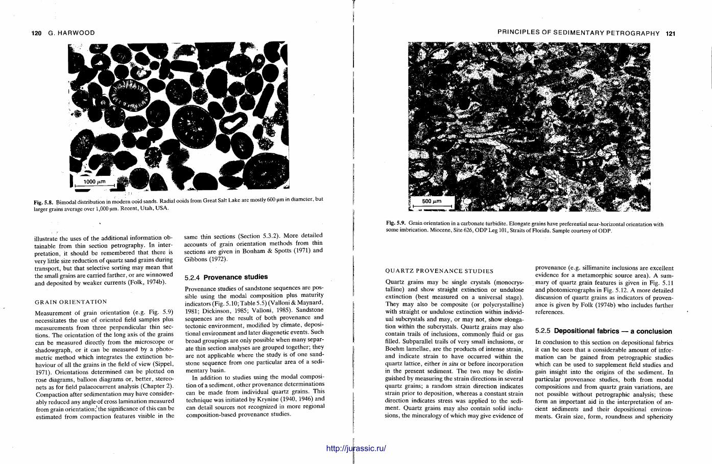
120 G. HARWOOD
Fig. 5.8. Bimodal distribution in modern ooid sands. Radial ooids from Great Salt Lake are mostly 600 urn in diameter, but larger grains average over 1,000 urn. Recent, Utah, USA.
illustrate the uses of the additional information obtainable from thin section petrography. In interpreta t ion, it should be r emembered that there is very little size reduction of quartz sand grains during t ransport , but that selective sorting may mean that the small grains are carried farther, or are winnowed and deposited by weaker currents (Folk, 1974b).
G R A I N O R I E N T A T I O N
Measurement of grain orientation (e.g. Fig. 5.9) necessitates the use of oriented field samples plus measurements from three perpendicular thin sections. T h e orientat ion of the long axis of the grains can be measured directly from the microscope or shadowgraph, or it can be measured by a photometric method which integrates the extinction behaviour of all the grains in the field of view (Sippel, 1971). Orientat ions determined can be plot ted on rose diagrams, balloon diagrams or, bet ter , s tereo-nets as for field palaeocurrent analysis (Chapter 2) . Compact ion after sedimentat ion may have considerably reduced any ang leof cross lamination measured from grain or ientat ion; ' the significance of this can be est imated from compaction features visible in the
same thin sections (Section 5.3.2). M o r e detailed accounts of grain orientation methods from thin sections are given in B o n h a m & Spotts (1971) and Gibbons (1972).
5.2.4 Provenance studies
Provenance studies of sandstone sequences are possible using the modal composit ion plus maturi ty indicators (Fig. 5.10; Table 5.5) (Valloni & Maynard , 1981; Dickinson, 1985; Valloni, 1985). Sandstone sequences are the result of both provenance and tectonic environment , modified by climate, depositional environment and later diagenetic events . Such broad groupings are only possible when many separate thin section analyses are grouped together ; they are not applicable where the study is of one sandstone sequence from one particular area of a sedimentary basin.
In addition to studies using the modal composition of a sediment , o ther provenance determinat ions can be made from individual quar tz grains. This technique was initiated by Krynine (1940, 1946) and can detail sources not recognized in more regional composit ion-based provenance studies.
PRINCIPLES OF SEDIMENTARY PETROGRAPHY 121
Fig. 5.9. Grain orientation in a carbonate turbidite. Elongate grains have preferential near-horizontal orientation with some imbrication. Miocene, Site 626, ODP Leg 101, Straits of Florida. Sample courtesy of ODP.
Q U A R T Z P R O V E N A N C E S T U D I E S
Quar tz grains may be single crystals (monocrys-talline) and show straight extinction or undulose extinction (best measured on a universal stage). They may also be composite (or polycrystalline) with straight or undulose extinction within individual subcrystals and may, or may not , show elongation within the subcrystals. Quar tz grains may also contain trails of inclusions, commonly fluid or gas filled. Subparallel trails of very small inclusions, or Boehm lamellae, are the products of intense strain, and indicate strain to have occurred within the quartz lattice, either in situ or before incorporation in the present sediment. T h e two. may be distinguished by measuring the strain directions in several quartz grains; a random strain direction indicates strain prior to deposit ion, whereas a constant strain direction indicates stress was applied to the sediment . Quar tz grains may also contain solid inclusions, the mineralogy of which may give evidence of
provenance (e.g. sillimanite inclusions are excellent evidence for a metamorphic source area) . A summary of quartz grain features is given in Fig. 5.11 and photomicrographs in Fig. 5.12. A more detailed discussion of quartz grains as indicators of provenance is given by Folk (1974b) who includes further references.
5.2.5 Depositional fabrics — a conclusion
In conclusion to this section on depositional fabrics it can be seen that a considerable amount of information can be gained from petrographic studies which can be used to supplement field studies and gain insight into the origins of the sediment . In particular provenance studies, both from modal compositions and from quartz grain variations, are not possible without petrographic analysis; these form an important aid in the interpretat ion of ancient sediments and their depositional environments . Grain size, form, roundness and sphericity
http://jurassic.ru/
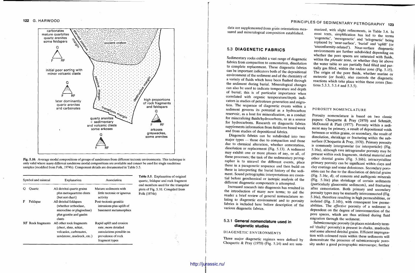
122 G. HARWOOD
Fig. 5.10. Average modal compositions of groups of sandstones from different tectonic environments. This technique is only valid where many different sandstone modal compositions are available and cannot be used for single sandstone samples (modified from Folk, 1974b). Component details are documented in Table 5.5.
Symbol and mineral Explanation Association
Q Quartz
F Feldspar
RF Rock fragments
All detrital quartz grains plus metaquartzite clasts (but not chert)
All detrital feldspars (whether orthoclase, microcline or plagioclase) plus granite and gneiss clasts
All other rock fragments (chert, slate, schist, volcanics, carbonates, sandstone, mudrock, etc.)
Mature sediments with little tectonic or igneous activity
Post-tectonic granitic intrusions plus uplift of basement metamorphics
Rapid uplift and erosion rate; more detailed associations possible on prevalence of rock fragment types
Table 5 . 5 . Explanation of original quartz, feldspar and rock fragment end members used for the triangular plots of Fig. 5.10. Compiled from Folk (1974b)
PRINCIPLES OF SEDIMENTARY PETROGRAPHY 123 data are supplemented from grain orientations measured and mineralogical composition established.
5.3 D I A G E N E T I C F A B R I C S
Sedimentary rocks exhibit a vast range of diagenetic fabrics from compaction to cementat ion, dissolution to complete replacement . These diagenetic fabrics can be important indicators both of the depositional environment of the sediment and of the chemistry of a variety of fluids which have been flushed through the sediment during burial . Mineralogical changes can also be used to indicate t empera ture and depth of burial; this is of particular importance when correlated with organic temperature /depth indicators in studies of petroleum generat ion and migration. The sequence of diagenetic events within a sediment governs its potential as a hydrocarbon reservoir, as a host for mineralization, as a conduit for mineralizing fluids/hydrocarbons, or as a source for hydrocarbons. Research on diagenetic fabrics supplements information from field/core based work and from studies of depositional fabrics.
Diagenetic fabrics can be subdivided into two major types — those due to compaction and those d u e t o chemical al terat ion, whether cementat ion, dissolution or replacement (Fig. 5.13). A sediment may exhibit one or more phases of any , or all, of these processes; the task of the sedimentary petrog-rapher is to unravel the different events, place these in a paragenetic sequence and then build on these in interpreting the burial history of the sediment . Sound petrographic interpretat ions are essential before geochemical or isotopic analysis of the different diagenetic components is a t tempted.
Increased research into diagenesis has resulted in the introduction of many new terms; to aid the reader a brief review of general nomenclature relating to diagenetic environment and to porosity fabrics is included here before description of the various diagenetic fabrics.
5.3.1 General nomenclature used in diagenetic studies
D I A G E N E T I C E N V I R O N M E N T S
Three major diagenetic regimes were defined by Choquet te & Pray (1970) (Fig. 5.14) and are sum
marized, with slight refinements, in Table 5.6. In most texts, simplification has led to the terms 'eogenetic ' , 'mesogenetic ' and ' telogenetic ' being replaced by 'near-surface ' , 'burial ' and 'uplift' (or 'unconformity-related ') . Near-surface diagenetic environments are further subdivided depending on whether the pore spaces are saturated with fluids, within the phreatic zone, or whether they lie above the water table so are partially fluid filled and partially gas filled, within the vadose zone (Fig. 5.15). The origin of the pore fluids, whether mar ine or meteor ic (or fresh), also controls the diagenetic reactions which take place within these zones (Sections 5.3.3, 5.3.4 and 5.3.5).
P O R O S I T Y N O M E N C L A T U R E
Porosity nomencla ture is based on two classic papers : Choque t t e & Pray (1970) and Schmidt, McDonald & Piatt (1977). Porosity within a sediment may be primary, a result of deposit ional voids between or within grains, or secondary, the result of dissolution, shrinkage or fracturing within the subsurface (Choquet te & Pray, 1970). Primary porosity is commonly intergranular (or interparticle) (Fig. 5.16a), al though rare intragranular porosity may be present within rock fragments, skeletal material and other detrital grains (Fig. 5.16b); intracrystalline primary porosity can be significant within clays and clay coatings and some dolostones. Secondary porosities can be due to the dissolution of detrital grains (Fig. 5.16c, d ) , of cements and authigenic minerals (Fig. 5.16e) plus shrinkage of certain sediments (particularly glauconitic sediments) , and fracturing after cementa t ion . Both primary and secondary porosity types may be mutually interconnected (Fig. 5.16a), therefore resulting in high permeabili t ies, or isolated (Fig. 5.16b), with consequent low permeabilities. The effective porosity of a sediment is dependent on the degree of interconnection of the pore spaces, which are thus utilized during fluid migration through the sediment.
Submicroscopic porosity (in places mistakenly termed 'chalky' porosity) is present in chalks, mudrocks and some altered detrital grains. Efficient impregnation with coloured resin within these sediments will demonst ra te the presence of submicroscopic porosity under a good pet rographic microscope; further
http://jurassic.ru/
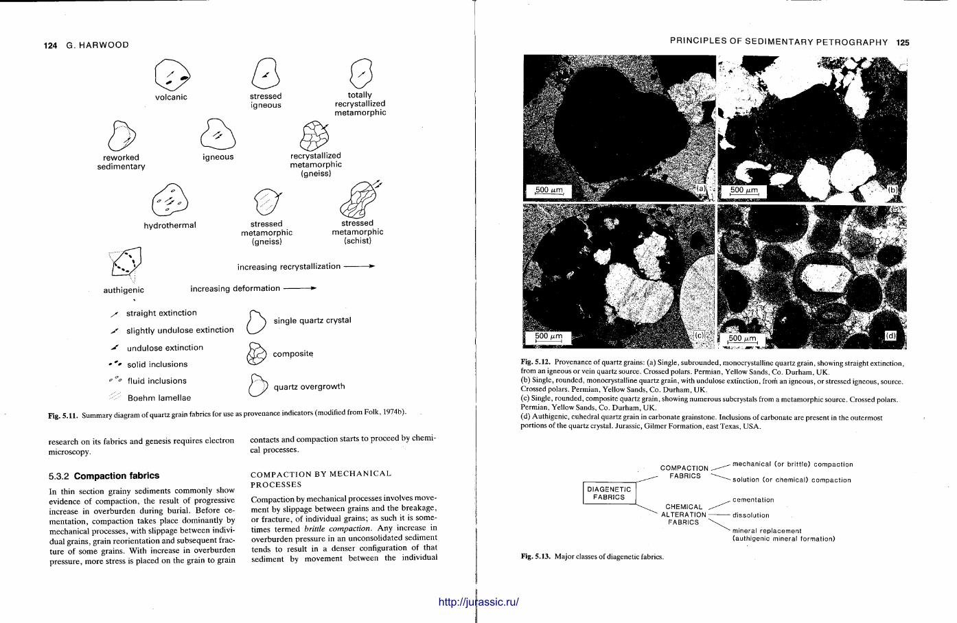
124 G. HARWOOD
volcanic stressed igneous
total ly recrystallized metamorphic
reworked sedimentary
igneous recrystallized metamorphic
(gneiss)
hydrothermal stressed metamorphic
(gneiss)
stressed metamorphic
(schist)
authigenic
increasing recrystall ization
increasing deformat ion *~
y straight ext inct ion
S sl ight ly undulose ext inct ion
undulose ext inct ion
• * * sol id inclusions
" ° a f lu id inclusions
: Boehm lamellae Fig. 5.11. Summary diagram of quartz grain fabrics for use as provenance indicators (modified from Folk, 1974b).
single quartz crystal
composi te
quartz overgrowth
research on its fabrics and genesis requires electron microscopy.
5.3.2 Compaction fabrics
In thin section grainy sediments commonly show evidence of compact ion, the result of progressive increase in overburden during burial. Before cementa t ion , compaction takes place dominantly by mechanical processes, with slippage between individual grains, grain reorientat ion and subsequent fracture of some grains. With increase in overburden pressure , more stress is placed on the grain to grain
contacts and compaction starts to proceed by chemical processes.
C O M P A C T I O N BY M E C H A N I C A L P R O C E S S E S
Compact ion by mechanical processes involves movement by slippage between grains and the breakage , or fracture, of individual grains; as such it is sometimes termed brittle compaction. Any increase in overburden pressure in an unconsolidated sediment tends to result in a denser configuration of that sediment by movement between the individual
PRINCIPLES OF SEDIMENTARY PETROGRAPHY 125
Fig. 5.12. Provenance of quartz grains: (a) Single, subrounded, monocrystalline quartz grain, showing straight extinction, from an igneous or vein quartz source. Crossed polars. Permian, Yellow Sands, Co. Durham, UK. (b) Single, rounded, monocrystalline quartz grain, with undulose extinction, from an igneous, or stressed igneous, source. Crossed polars. Permian, Yellow Sands, Co. Durham, UK. (c) Single, rounded, composite quartz grain, showing numerous subcrystals from a metamorphic source. Crossed polars. Permian, Yellow Sands, Co. Durham, UK. (d) Authigenic, euhedral quartz grain in carbonate grainstone. Inclusions of carbonate are present in the outermost portions of the quartz crystal. Jurassic, Gilmer Formation, east Texas, USA.
D I A G E N E T I C F A B R I C S
C O M P A C T I O N F A B R I C S
C H E M I C A L . A L T E R A T I O N -
F A B R I C S
• m e c h a n i c a l ( o r b r i t t l e ) c o m p a c t i o n
s o l u t i o n ( o r c h e m i c a l ) c o m p a c t i o n
. c e m e n t a t i o n
d i s s o l u t i o n
• m i n e r a l r e p l a c e m e n t ( a u t h i g e n i c m i n e r a l f o r m a t i o n )
Fig. 5.13. Major classes of diagenetic fabrics.
http://jurassic.ru/
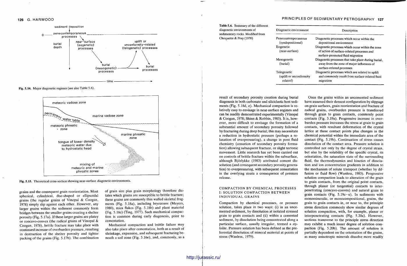
126 G. HARWOOD
s e d i m e n t d e p o s i t i o n
I p e n e c o n t e m p o r a n e o u s _
p r o c e s s e s \ ^
bur ia l d e p t h
n e a r - s u r f a c e ( e o g e n e t i c ) p r o c e s s e s
uplift or u n c o n f o r m i t y - r e l a t e d
( t e l o g e n e t i c ) p r o c e s s e s
burial ( m e s o g e n e t i c )
p r o c e s s e s
t i m e
Fig. 5.14. Major diagenetic regimes (see also Table 5.6).
mixing of meteoric and marine
phreatic zones
Fig. 5.15. Theoretical cross-section showing near-surface diagenetic environments.
grains and the consequent grain reorientat ion. Most spherical, cylindrical, disc-shaped or ellipsoidal grains (the regular grains of Vinopal & Coogan, 1978) simply slip against each other . However , any larger grains within the sediment commonly form bridges between the smaller grains creating a shelter porosity (Fig. 5.17a). If these larger grains are platey o r concavo-convex ( the radical grains of Vinopal & Coogan, 1978), brittle fracture may take place with continued increase of overburden pressure, resulting in destruction of the shelter porosity and tighter packing of the grains (Fig. 5.17b). The combination
of grain size plus grain morphology therefore dictates which grains are susceptible to brit t le fracture; these grains are commonly thin walled skeletal fragments (Fig. 5.18a), including bryozoans (Meyers , 1980), mica flakes (Fig. 5.18b) and plant material (Fig. 5.18c) (Ting, 1977). Such mechanical compaction is common during early diagenesis, prior to cementat ion.
Mechanical compaction and brittle failure may also take place after cementat ion, both as a result of shr inkage, expansion, and subsequent fracturing beneath a soil zone (Fig. 5.16e), and, commonly , as a
PRINCIPLES OF SEDIMENTARY PETROGRAPHY 127
Table 5.6. Summary of the different diagenetic environments of sedimentary rocks. Modified from Choquette & Pray (1970)
Diagenetic environment Description
Penecontemporaneous Diagenetic processes which occur within the (syndepositional) depositional environment
Eogenetic Diagenetic processes which occur within the zone (near-surface) of action of surface-related processes and
surface-promoted fluid migration Mesogenetic Diagenetic processes that take place during burial,
(burial) away from the zone of major influences of surface-related processes
Telogenetic Diagenetic processes which are related to uplift (uplift or unconformity and commonly result from surface-related fluid
related) migration
result of secondary porosity creation during burial diagenesis in both carbonate and siliciclastic host sediments (Fig. 5.18d, e ) . Mechanical compaction is relatively easy to envisage in near-surface regimes and can be readily demonstrated experimentally (Vinopal & Coogan , 1978; Shinn & Robbin , 1983). It is, however, more difficult to envisage the formation of a substantial amount of secondary porosity followed by fracturing during deep burial; this may necessitate a reduction in hydrostatic pressure (perhaps a relaxation of overpressuring), a change in pore fluid chemistry (cessation of secondary porosity formation) allowing subsequent fracture, or slight tectonic movement . Little research has yet been carried out on controls of brittle fracture within the subsurface, al though Bjorlykke (1983) at tr ibuted cement dissolution (and consequent secondary porosity generation) to overpressuring, with subsequent cementation in the overlying strata a consequence of pressure release.
C O M P A C T I O N BY C H E M I C A L P R O C E S S E S I: S O L U T I O N C O M P A C T I O N B E T W E E N I N D I V I D U A L G R A I N S
Compact ion by chemical processes, or pressure solution, takes place in two ways: (i) in an uncemented sediment , by dissolution at isolated stressed grain to grain contacts and (ii) within a cemented sediment , by dissolution being concentrated along a particular surface, usually irregular, te rmed a sty-lolite. Pressure solution has been defined as the preferential dissolution of mineral material at points of stress (Wanless, 1979).
Once the grains within an uncemented sediment have assumed their densest configuration by slippage on grain surfaces, grain reorientat ion and fracture of radical grains, overburden pressure is transferred through grain to grain contacts , commonly point contacts (Fig. 5.19a). Progressive increase in overburden pressure increases the stress at grain to grain contacts, with resultant deformation of the crystal lattice at these contact points plus changes in the chemical potential within the immediate area of the contact (Fig. 5.19b). Cont inuat ion of stress causes dissolution of the contact area. Pressure solution is controlled not only by the degree of crystal strain, but also by the solubility of the specific crystal, its or ientat ion, the saturation state of the surrounding fluid, the thermodynamics and kinetics of dissolution and ion concentrat ion gradients in addition to the mechanism of solute t ransport (whether by diffusion or fluid flow) (Wanless, 1983). Progressive solution compaction leads to alteration of the grain to grain contacts, from the original point contacts, through planar (or tangential) contacts to interpenetrat ing (concavo-convex) and sutural grain to grain contacts (Fig. 5.19c—e). In sediments with monomineral ic , or monocomposi t ional , grains, the grain to grain contacts in, or near t o , the principle stress direction commonly show similar degrees of solution compact ion, with, for example, planar or interpenetrat ing contacts (Fig. 5.20a). However , sections transverse to the principle stress direction may exhibit a much lesser degree of solution compaction (Fig. 5.20b). The amount of solution is partially dependent on the orientation of the grains, as many anisotropic minerals dissolve more readily
llllllllll http://jurassic.ru/
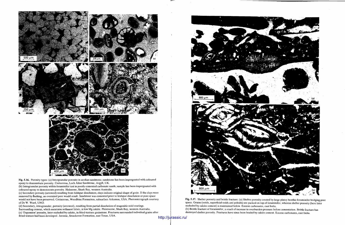
Fig. 5.16. Porosity types: (a) Intergranular porosity in aeolian sandstone; sandstone has been impregnated with coloured epoxy to demonstrate porosity. Cretaceous, Loch Aline Sandstone, Argyll, UK. (b) Intragranular porosity within foraminifer test in poorly cemented carbonate sands; sample has been impregnated with coloured epoxy to demonstrate porosity. Holocene, Shark Bay, western Australia. (c) Secondary porosity (arrowed) resulting from feldspar dissolution; clays indicate original shape of grain. If the clays were removed by flushing, an oversized pore would result. Sandstone was cemented prior to feldspar dissolution or pore space would not have been preserved. Cretaceous, Woodbine Formation, subsurface Arkansas, USA. Photomicrograph courtesy ofDrW. Ward, UNO. (d) Secondary, intragranular, porosity (arrowed), resulting from partial dissolution of aragonitic ooid coatings. Surrounding cement, which maintains sediment fabric, is low Mg calcite. Pleistocene, Shark Bay, western Australia. (e) 'Expansion' porosity, later occluded by calcite, in fitted-texture grainstone. Fractures surrounded individual grains after fitted-texture had been developed. Jurassic, Smackover Formation, east Texas, USA.
aiiiiiiiiiiiiiiiiiiiiiiiiii
Fig. 5.17. Shelter porosity and brittle fracture: (a) Shelter porosity created by large platey benthic foraminifer bridging pore space. Grains (ooids, superficial ooids and peloids) are packed on top of foraminifer, whereas shelter porosity (here later occluded by calcite cement) is maintained below. Eocene carbonates, east India. (b) Brittle fracture of foraminifer, a result of increase in overburden pressure before cementation. Brittle fracture has destroyed shelter porosity. Fractures have since been healed by calcite cement. Eocene carbonates, east India.
http://jurassic.ru/
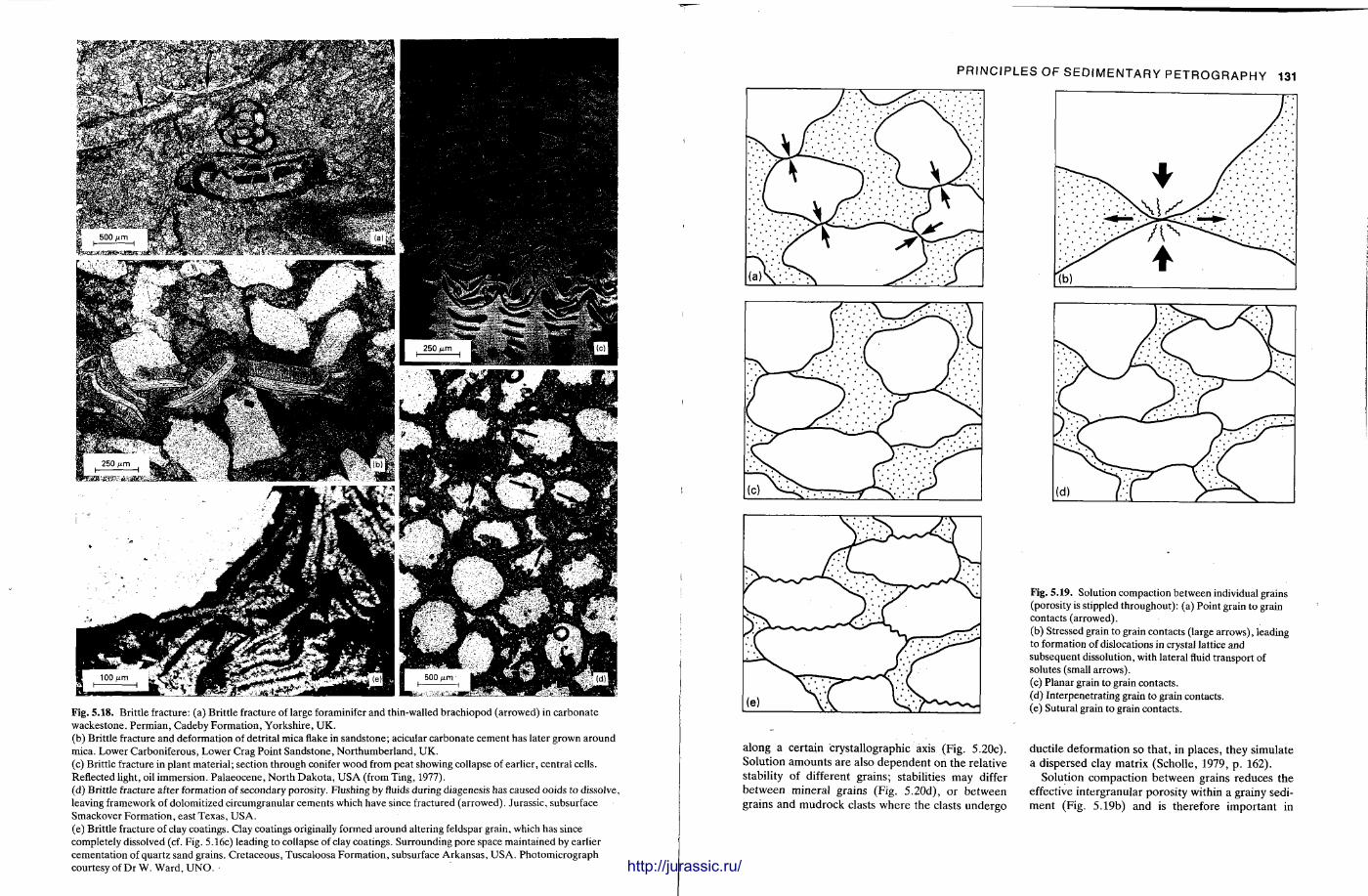
Fig. 5.18. Brittle fracture: (a) Brittle fracture of large foraminifer and thin-walled brachiopod (arrowed) in carbonate wackestone. Permian, Cadeby Formation, Yorkshire, UK. (b) Brittle fracture and deformation of detrital mica flake in sandstone; acicular carbonate cement has later grown around mica. Lower Carboniferous, Lower Crag Point Sandstone, Northumberland, UK. (c) Brittle fracture in plant material; section through conifer wood from peat showing collapse of earlier, central cells. Reflected light, oil immersion. Palaeocene, North Dakota, USA (from Ting, 1977). (d) Brittle fracture after formation of secondary porosity. Flushing by fluids during diagenesis has caused ooids to dissolve, leaving framework of dolomitized circumgranular cements which have since fractured (arrowed). Jurassic, subsurface Smackover Formation, east Texas, USA. (e) Brittle fracture of clay coatings. Clay coatings originally formed around altering feldspar grain, which has since completely dissolved (cf. Fig. 5.16c) leading to collapse of clay coatings. Surrounding pore space maintained by earlier cementation of quartz sand grains. Cretaceous, Tuscaloosa Formation, subsurface Arkansas, USA. Photomicrograph courtesy of Dr W. Ward, UNO.
PRINCIPLES OF SEDIMENTARY PETROGRAPHY 131
along a certain crystallographic axis (Fig. 5.20c). Solution amounts are also dependent on the relative stability of different grains; stabilities may differ between mineral grains (Fig. 5.20d), or between grains and mudrock clasts where the clasts undergo
Fig. 5.19. Solution compaction between individual grains (porosity is stippled throughout): (a) Point grain to grain contacts (arrowed). (b) Stressed grain to grain contacts (large arrows), leading to formation of dislocations in crystal lattice and subsequent dissolution, with lateral fluid transport of solutes (small arrows). (c) Planar grain to grain contacts. (d) Interpenetrating grain to grain contacts. (e) Sutural grain to grain contacts.
ductile deformation so that , in places, they simulate a dispersed clay matrix (Scholle, 1979, p . 162).
Solution compaction between grains reduces the effective intergranular porosity within a grainy sediment (Fig. 5.19b) and is therefore important in
illilll http://jurassic.ru/
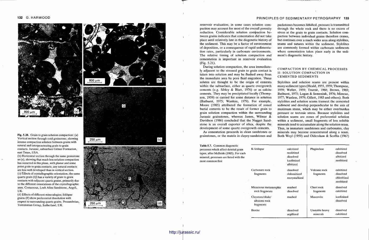
132 G. HARWOOD
800 /j,m
Fig. 5.20. Grain to grain solution compaction: (a) Vertical section through ooid grainstone, showing intense compaction solution between grains with sutural and interpenetrating grain to grain contacts. Jurassic, subsurface Gilmer Formation, east Texas, USA. (b) Horizontal section through the same grainstone as (a), showing that much less solution compaction has occurred in this plane, with planar and some point grain to grain contacts; any sutural contacts are less well developed than in vertical section. (c) Effects of crystallographic orientation; the same quartz grain (Q) has a variety of grain to grain contacts with adjacent quartz grains, primarily due to the different orientations of the crystallographic axes. Cretaceous, Loch Aline Sandstone, Argyll, UK. (d) Effects of different mineralogies; feldspar grains (F) show preferential dissolution with respect to surrounding quartz grains. Precambrian, Torridonian Group, Sutherland, UK.
PRINCIPLES OF SEDIMENTARY PETROGRAPHY 133
reservoir evaluation; in some cases solution compaction may account for most of the overall porosity reduction. Considerable solution compaction between grains indicates that cementat ion did not take place until relatively late in the diagenetic history of the sediment. This may be a factor of environment of deposit ion, or a consequence of rapid sedimentation rates, particularly in carbonate environments . The relative timing of solution compaction and cementat ion is important in reservoir evaluation (Fig. 5.21).
Dur ing solution compact ion, the area immediately adjacent to the stressed grain to grain contact is taken into solution and may be flushed away from the immediate area by pore fluid migration. These solutes are thought to be the origin of cements within the subsurface, either as quar tz overgrowth cements (e.g. Sibley & Blatt , 1976) or as calcite cements . They may be precipitated locally (Thompson, 1959) or carried for some distance in solution (Bathurst , 1975; Wanless , 1979). For example, Moore (1985) at t r ibuted the formation of zoned burial cements to be the result of former grain to grain solution compaction within the surrounding Jurassic grainstones, whereas James , Wilmar & Davidson (1986) concluded that the Nugget Sandstone is an overall exporter of silica, despite the development of some quar tz overgrowth cements .
As cementat ion proceeds in clean sandstones or grainstones, or the matrix in clayey-sandstones and
packstones becomes lithified, pressure is transmitted through the whole rock and there is no excess of stress at the grain to grain contacts. Solution compaction between individual grains therefore ceases, but continues over a much wider area along stylolites, seams and sutures within the sediment. Stylolites are commonly formed within carbonate sediments where cementat ion takes place early in the sediment ' s diagenetic history.
C O M P A C T I O N BY C H E M I C A L P R O C E S S E S I I : S O L U T I O N C O M P A C T I O N IN C E M E N T E D S E D I M E N T S
Stylolites and solution seams are present within many sediment types (Heald , 1955,1959; Thompson , 1959; Weller, 1959; Trurni t , 1968; Brown, 1969; Bathurs t , 1975; Logan & Semeniuk, 1976; Mimran , 1977; Wanless , 1979; Gillett , 1983 and others) . Both stylolites and solution seams transect the cemented sediment and develop perpendicular to the axis of maximum stress, which may be either overburden pressure or tectonic stress. Because stylolites and solution seams are zones of preferential solution within a sediment , small fragments of less soluble minerals tend to accumulate along the solution seam. Thus , in immature sandstones and carbonates , clay minerals may become concentrated along a seam. Both Weyl (1959) and Oldershaw & Scoffin (1967)
Table 5.7. Common diagenetic processes which affect detrital grain types, after McBride (1985). For each mineral, processes are listed with the most common first
K-feldspar calcitized zeolitized dissolved kaolinized albitized
Plagioclase calcitized dissolved albitized zeolitized
Carbonate rock fragments
dissolved dolomitized recrystallized
Volcanic rock fragments
calcitized dissolved chloritized zeolitized
Micaceous metamorphic rock fragments
mashed dissolved
Chert rock fragments
dissolved calcitized
Claystone/shale/ siltstone rock fragments
mashed Muscovite kaolinized dissolved
Biotite dissolved argillized
Unstable heavy minerals
dissolved calcitized
ill http://jurassic.ru/
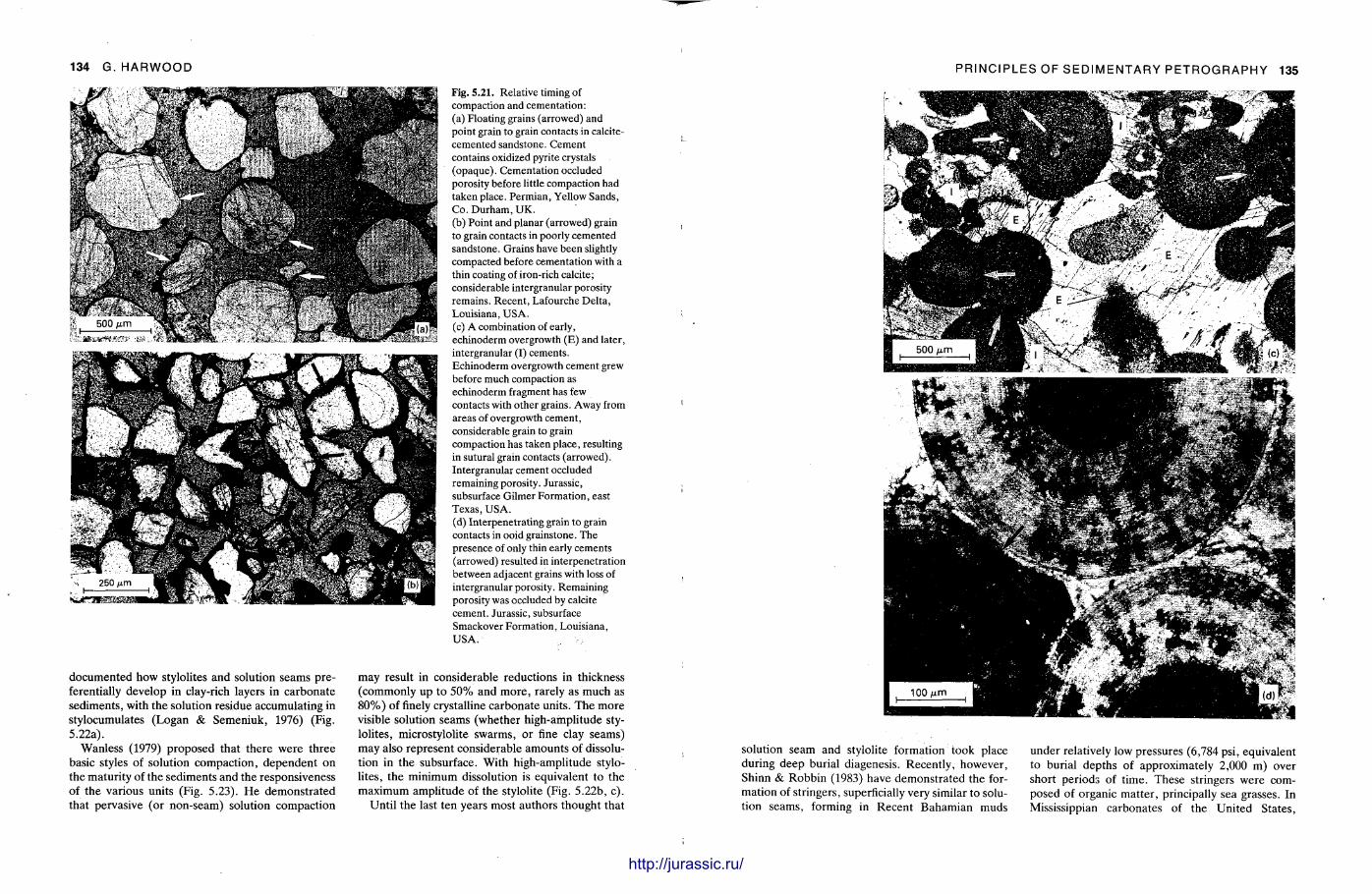
134 G. HARWOOD
Fig. 5.21. Relative timing of compaction and cementation: (a) Floating grains (arrowed) and point grain to grain contacts in calcite-cemented sandstone. Cement contains oxidized pyrite crystals (opaque). Cementation occluded porosity before little compaction had taken place. Permian, Yellow Sands, Co. Durham, UK. (b) Point and planar (arrowed) grain to grain contacts in poorly cemented sandstone. Grains have been slightly compacted before cementation with a thin coating of iron-rich calcite; considerable intergranular porosity remains. Recent, Lafourche Delta, Louisiana, USA. (c) A combination of early, echinoderm overgrowth (E) and later, intergranular (I) cements. Echinoderm overgrowth cement grew before much compaction as echinoderm fragment has few contacts with other grains. Away from areas of overgrowth cement, considerable grain to grain compaction has taken place, resulting in sutural grain contacts (arrowed). Intergranular cement occluded remaining porosity. Jurassic, subsurface Gilmer Formation, east Texas, USA. (d) Interpenetrating grain to grain contacts in ooid grainstone. The presence of only thin early cements (arrowed) resulted in interpenetration between adjacent grains with loss of intergranular porosity. Remaining porosity was occluded by calcite cement. Jurassic, subsurface Smackover Formation, Louisiana, USA.
documented how stylolites and solution seams preferentially develop in clay-rich layers in carbonate sediments , with the solution residue accumulating in stylocumulates (Logan & Semeniuk, 1976) (Fig. 5.22a).
Wanless (1979) proposed that there were three basic styles of solution compact ion, dependent on the maturity of the sediments and the responsiveness of the various units (Fig. 5.23). H e demons t ra ted that pervasive (or non-seam) solution compaction
may result in considerable reductions in thickness (commonly up to 5 0 % and more , rarely as much as 80%) of finely crystalline carbonate units. T h e more visible solution seams (whether high-amplitude stylolites, microstylolite swarms, or fine clay seams) may also represent considerable amounts of dissolution in the subsurface. With high-amplitude stylolites, the minimum dissolution is equivalent to the maximum ampli tude of the stylolite (Fig. 5.22b, c) .
Unti l the last ten years most authors thought that
PRINCIPLES OF SEDIMENTARY PETROGRAPHY 135
solution seam and stylolite formation took place during deep burial diagenesis. Recently, however , Shinn & Robbin (1983) have demonst ra ted the formation of stringers, superficially very similar to solution seams, forming in Recent Bahamian muds
under relatively low pressures (6,784 psi, equivalent to burial depths of approximately 2,000 m) over short periods of t ime. These stringers were composed of organic mat ter , principally sea grasses. In Mississippian carbonates of the United States,
llllll
http://jurassic.ru/
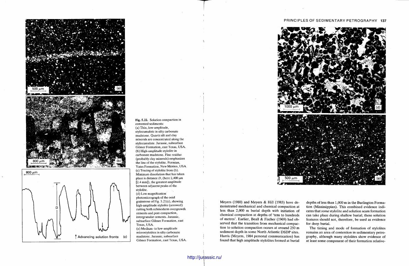
Fig. 5.22. Solution compaction in cemented sediments: (a) Thin, low-amplitude, stylocumulate in silty carbonate mudstone. Quartz silt and clay minerals are concentrated along the stylocumulate. Jurassic, subsurface Gilmer Formation, east Texas, USA. (b) High-amplitude stylolite in carbonate mudstone. Fine residue (probably clay minerals) emphasizes the line of the stylolite. Permian, Yates Formation, New Mexico, USA. (c) Tracing of stylolite from (b). Minimum dissolution that has taken place is distance D , (here 2,400 urn [2.4 mm]), the greatest amplitude between adjacent peaks of the stylolite. (d) Low magnification photomicrograph of the ooid grainstone of Fig. 5.21(c), showing high-amplitude stylolite (arrowed) cutting both echinoderm overgrowth cements and post-compaction, intergranular cements. Jurassic, subsurface Gilmer Formation, east Texas, USA. (e) Medium- to low-amplitude microstylolites in silty carbonate mudstone. Jurassic, subsurface Gilmer Formation, east Texas, USA.
fMWtiHHHHIItHlimttlllllttlimHHWMtlHttHtiiHHIl
PRINCIPLES OF SEDIMENTARY PETROGRAPHY 137
Meyers (1980) and Meyers & Hill (1983) have demonst ra ted mechanical and chemical compact ion at less than 2,000 m burial depth with initiation of chemical compaction at depths of ' tens to hundreds of metres ' . Earl ier , Beall & Fischer (1969) had observed that the transition from mechanical compaction to solution compaction occurs at a round 250 m sediment depth in some North Atlantic D S D P sites. Harr is (Meyers , 1984 personal communicat ion) has found that high ampli tude stylolites formed at burial
depths of less than 1,000 m in the Burlington Formation (Mississippian). This combined evidence indicates that some stylolite and solution seam formation can take place during shallow burial; these solution features should not , therefore, be used as evidence for deep burial.
The timing and mode of formation of stylolites remains a n area of contention in sedimentary petrography, al though many stylolites show evidence of at least some component of their formation relative-
It, ''Wllllllllllilll http://jurassic.ru/
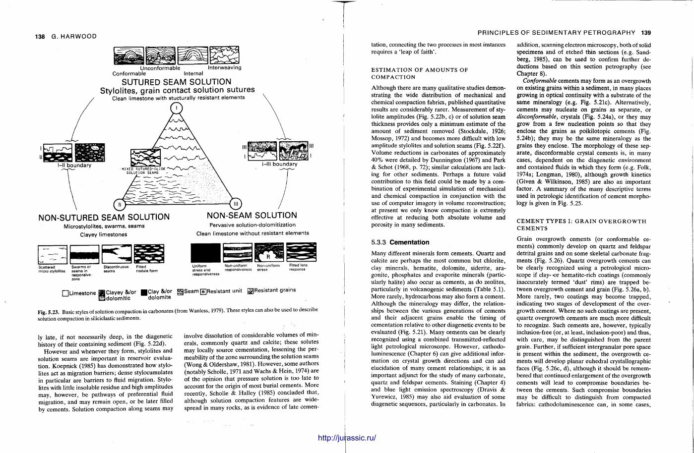
138 G. HARWOOD
Unconformable Interweaving Conformable Internal
SUTURED SEAM SOLUTION Stylolites, grain contact solution sutures
Clean limestone with stucturally resistant elements
-III boundary
NON-SUTURED SEAM SOLUTION Microstylolites, swarms, seams
Clayey limestones
Scattered Swarms or micro stylolites seams in
responsive zone
NON-SEAM SOLUTION Pervasive solution-dolomitization
Clean limestone without resistant elements
Uni form Non-uni form stress and responsiveness responsiveness
• Limestone ^ C l a y e y &/or g C l a y &/or g jSeam rjTJResistant unit ^Res is tant grains HSdolomitic dolomite
Fig. 5.23. Basic styles of solution compaction in carbonates (from Wanless, 1979). These styles can also be used to describe solution compaction in siliciclastic sediments.
ly la te , if not necessarily deep , in the diagenetic history of their containing sediment (Fig. 5.22d).
However and whenever they form, stylolites and solution seams are impor tant in reservoir evaluat ion. Koepnick (1985) has demonst ra ted how stylolites act as migration barriers; dense stylocumulates in particular are barriers to fluid migrat ion. Stylolites with little insoluble residue and high ampli tudes may, however , be pathways of preferential fluid migrat ion, and may remain open , or be later filled by cements . Solution compaction along seams may
involve dissolution of considerable volumes of minerals, commonly quar tz and calcite; these solutes may locally source cementa t ion , lessening the permeabili ty of the zone surrounding the solution seams (Wong & Oldershaw, 1981). However , some authors (notably Scholle, 1971 and Wachs & He in , 1974) a re of the opinion that pressure solution is too late to account for the origin of most burial cements . M o r e recently, Scholle & Halley (1985) concluded that , al though solution compaction features are widespread in many rocks, as is evidence of late cemen-
PRINCIPLES OF SEDIMENTARY PETROGRAPHY 139
tation, connecting the two processes in most instances requires a ' leap of faith' .
E S T I M A T I O N O F A M O U N T S O F C O M P A C T I O N
Although the re are many qualitative studies demonstrating the wide distribution of mechanical and chemical compaction fabrics, published quanti tat ive results are considerably rarer . Measurement of stylolite ampli tudes (Fig. 5.22b, c) or of solution seam thickness provides only a minimum estimate of the amount of sediment removed (Stockdale, 1926; Mossop, 1972) and becomes more difficult with low ampli tude stylolites and solution seams (Fig. 5.22f). Volume reductions in carbonates of approximately 4 0 % were detailed by Dunnington (1967) and Park & Schot (1968, p . 72); similar calculations are lacking for o ther sediments . Perhaps a future valid contribution to this field could be made by a combination of experimental simulation of mechanical and chemical compaction in conjunction with the use of computer imagery in volume reconstruction; at present we only know compaction is extremely effective at reducing both absolute volume and porosity in many sediments .
5.3.3 Cementation
Many different minerals form cements . Quar tz and calcite are perhaps the most common but chlorite, clay minerals , hemat i te , dolomite , siderite, aragonite , phosphates and evapori te minerals (particularly halite) also occur as cements , as do zeolites, particularly in volcanogenic sediments (Table 5.1). More rarely, hydrocarbons may also form a cement . Al though the mineralogy may differ, the relationships between the various generat ions of cements and their adjacent grains enable the timing of cementat ion relative to o ther diagenetic events to be evaluated (Fig. 5.21). Many cements can be clearly recognized using a combined transmitted-reflected light petrological microscope. However , cathodoluminescence (Chapter 6) can give additional information on crystal growth directions and can aid elucidation of many cement relationships; it is an important adjunct for the study of many carbonate , quar tz and feldspar cements . Staining (Chapter 4) and blue light emission spectroscopy (Dravis & Yurewicz, 1985) may also aid evaluation of some diagenetic sequences , particularly in carbonates . In
addit ion, scanning electron microscopy, both of solid specimens and of etched thin sections (e.g. Sand-berg, 1985), can be used to confirm further deductions based on thin section pet rography (see Chapter 8) .
Conformable cements may form as an overgrowth on existing grains within a sediment , in many places growing in optical continuity with a substrate of the same mineralogy (e.g. Fig. 5.21c). Alternatively, cements may nucleate on grains as separa te , or disconformable, crystals (Fig. 5.24a), or they may grow from a few nucleation points so that they enclose the grains as poikilotopic cements (Fig. 5.24b); they may be the same mineralogy as the grains they enclose. The morphology of these separa te , disconformable crystal cements is, in many cases, dependent on the diagenetic environment and contained fluids in which they form (e.g. Folk, 1974a; Longman , 1980), al though growth kinetics (Given & Wilkinson, 1985) are also an important factor. A summary of the many descriptive terms used in petrologic identification of cement morphology is given in Fig. 5.25.
C E M E N T T Y P E S I: G R A I N O V E R G R O W T H C E M E N T S
Grain overgrowth cements (or conformable cements) commonly develop on quar tz and feldspar detrital grains and on some skeletal carbonate fragments (Fig. 5.26). Quar tz overgrowth cements can be clearly recognized using a petrological microscope if clay- o r hematite-rich coatings (commonly inaccurately te rmed 'dust ' rims) are t rapped between overgrowth cement and grain (Fig. 5.26a, b) . M o r e rarely, two coatings may become t rapped , indicating two stages of development of the overgrowth cement . W h e r e no such coatings are present , quartz overgrowth cements are much more difficult to recognize. Such cements are , however , typically inclusion-free (or , at least, inclusion-poor) and thus , with care , may be distinguished from the parent grain. Fur ther , if sufficient intergranular pore space is present within the sediment , the overgrowth cements will develop planar euhedral crystallographic faces (Fig. 5.26c, d ) , al though it should b e remembered that continued enlargement of the overgrowth cements will lead to compromise boundaries between the cements . Such compromise boundaries may be difficult to distinguish from compacted fabrics: cathodoluminescence can, in some cases,
http://jurassic.ru/
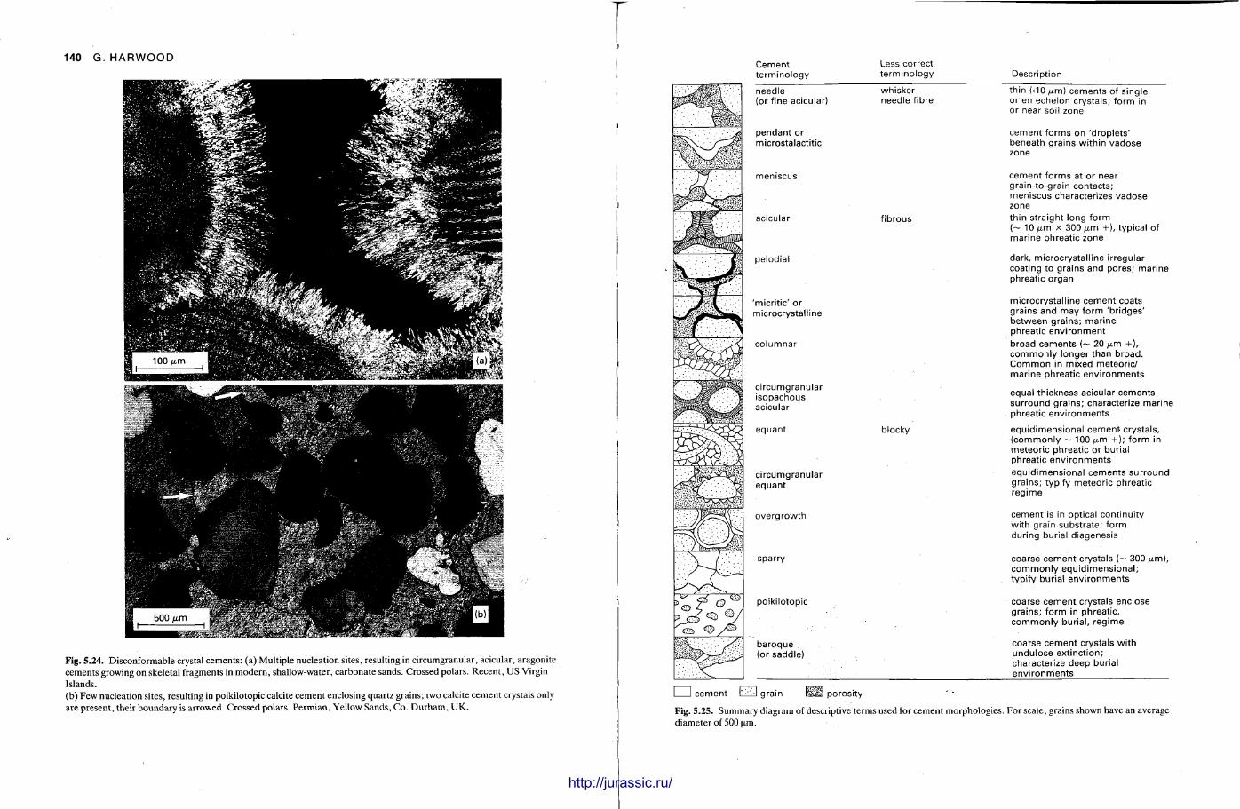
140 G. HARWOOD
Fig. 5.24. Disconformable crystal cements: (a) Multiple nucleation sites, resulting in circumgranular, acicular, aragonite cements growing on skeletal fragments in modern, shallow-water, carbonate sands. Crossed polars. Recent, US Virgin Islands. (b) Few nucleation sites, resulting in poikilotopic calcite cement enclosing quartz grains; two calcite cement crystals only are present, their boundary is arrowed. Crossed polars. Permian, Yellow Sands, Co. Durham, UK.
Cement terminology
Less correct terminology Description
needle (or fine acicular)
pendant or microstalactitic
whisker needle fibre
fibrous
pelodial
'micritic' or microcrystalline
columnar
circumgranular isopachous acicular
equant
circumgranular equant
overg rowth
sparry
poikilotopic
baroque (or saddle)
blocky
thin (do /xm) cements of single or en echelon crystals; form in or near soil zone
cement forms on 'droplets' beneath grains within vadose zone
cement forms at or near grain-to-grain contacts; meniscus characterizes vadose zone thin straight long form (~ 10 / u m x 300 x i m +), typical of marine phreatic zone
dark, microcrystalline irregular coating to grains and pores; marine phreatic organ
microcrystalline cement coats grains and may form 'bridges' between grains; marine phreatic environment broad cements (~ 20 /xm +), commonly longer than broad. Common in mixed meteoric/ marine phreatic environments
equal thickness acicular cements surround grains; characterize marine phreatic environments
equidimensional cement crystals, (commonly ~ 100 / x m +); form in meteoric phreatic or burial phreatic environments equidimensional cements surround grains; typify meteoric phreatic regime
cement is in optical continuity with grain substrate; form during burial diagenesis
coarse cement crystals (~ 300 /xm), commonly equidimensional; typify burial environments
coarse cement crystals enclose grains; form in phreatic, commonly burial, regime
coarse cement crystals with undulose extinction; characterize deep burial environments
cement grain porosity
Fig. 5.25. Summary diagram of descriptive terms used for cement morphologies. For scale, grains shown have an average diameter of 500 urn.
http://jurassic.ru/
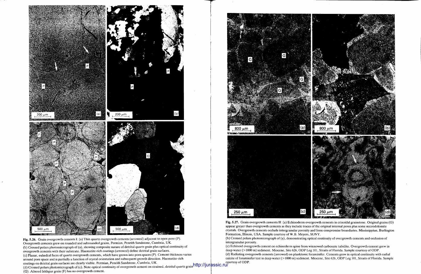
Fig. 5.26. Grain overgrowth cements I: (a) Thin quartz overgrowth cements (arrowed) adjacent to open pore (P). Overgrowth cements grew on rounded and subrounded grains, Permian, Penrith Sandstone, Cumbria, UK. (b) Crossed polars photomicrograph of (a), showing composite nature of detrital quartz grain plus optical continuity of overgrowth cements with their substrate. Haematite-rich coatings (arrowed) define detrital grain surfaces. (c) Planar, euhedral faces of quartz overgrowth cements, which have grown into pore.spaces (P). Cement thickness varies around pore space and is partially a function of crystal orientation and subsequent growth direction. Haematite-rich coatings on detrital grain surfaces are clearly visible. Permian, Penrith Sandstone, Cumbria, UK. (d) Crossed polars photomicrograph of (c). Note optical continuity of overgrowth cement on strained, detrital quartz grain (Q). Altered feldspar grain (F) has no overgrowth cement.
•itiiimmmmmi
Fig. 5.27. Grain overgrowth cements II: (a) Echinoderm overgrowth cements in crinoidal grainstone. Original grains (G) appear greyer than overgrowth cements as they include traces of the original internal pores plus some microdolomite crystals. Overgrowth cements occlude intergranular porosity and form compromise boundaries. Mississippian, Burlington Formation, Illinois, USA. Sample courtesy of W.B. Meyers, SUNY. (b) Crossed polars photomicrograph of (a), demonstrating optical continuity of overgrowth cements and occlusion of intergranular porosity. (c) Echinoid overgrowth cement on echinoderm spine from winnowed carbonate tubidite. Overgrowth cement grew in deep water (>1000 m) sediment. Miocene, Site 626, ODP Leg 101, Straits of Florida. Sample courtesy of ODP. (d) Radiating overgrowth cements (arrowed) on planktonic foraminifer. Cements grow in optical continuity with radial calcite of foraminifer test in deep water (>1000 m) sediment. Miocene, Site 626, ODP Leg 101, Straits of Florida. Sample courtesy of ODP. http://jurassic.ru/
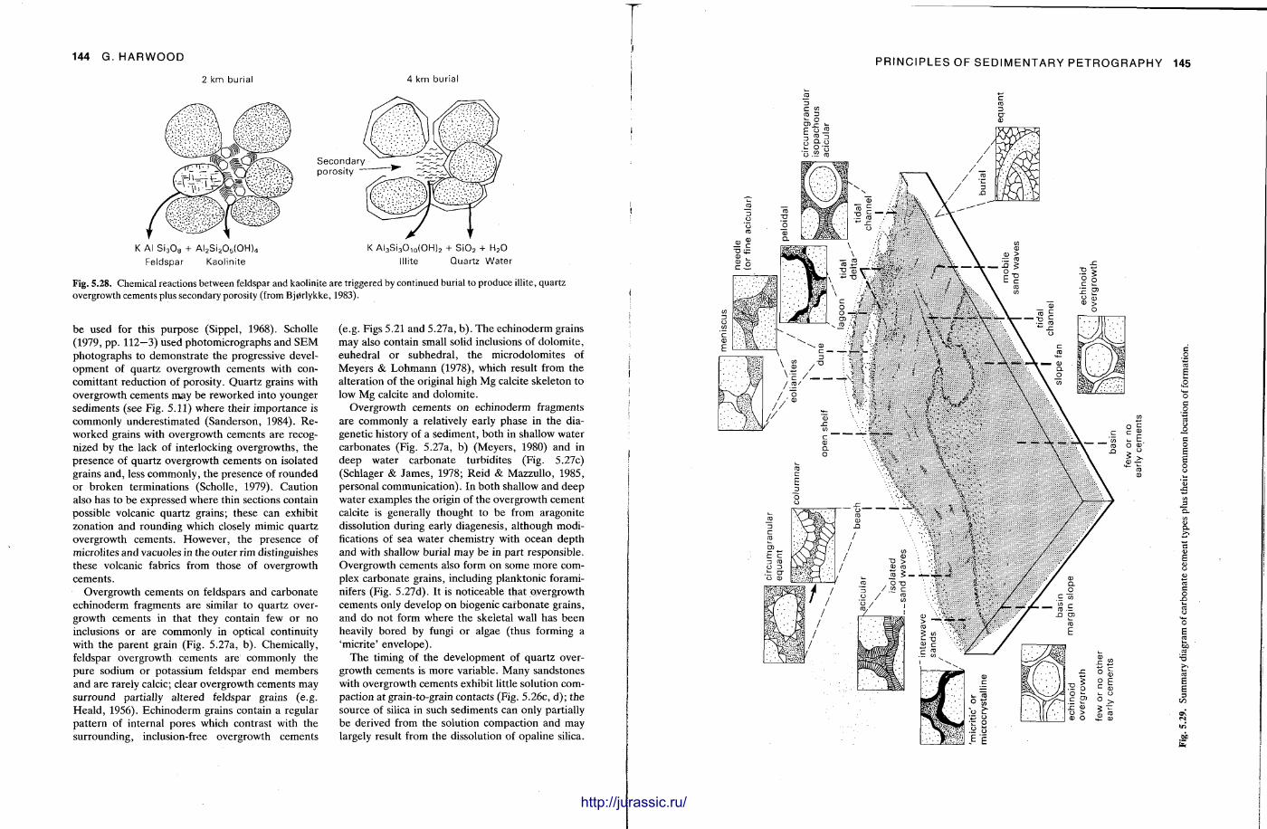
144 G. HARWOOD
2 km burial 4 km burial
K Al S i 3 0 8 + AI 2 Si 2 0 5 (OH) 4
Feldspar Kaolinite
Secondary porosity
K AI 3 Si 3 O 1 0 (OH) 2 + S i 0 2 + H 2 0 lllite Quartz Water
Fig. 5.28. Chemical reactions between feldspar and kaolinite are triggered by continued burial to produce illite, quartz overgrowth cements plus secondary porosity (from Bj0rlykke, 1983).
be used for this purpose (Sippel, 1968). Scholle (1979, pp . 112—3) used photomicrographs and S E M photographs to demonst ra te the progressive development of quar tz overgrowth cements with concomit tant reduction of porosity. Quar tz grains with overgrowth cements may be reworked into younger sediments (see Fig. 5.11) where their impor tance is commonly underes t imated (Sanderson, 1984). R e worked grains with overgrowth cements are recognized by the lack of interlocking overgrowths, the presence of quar tz overgrowth cements on isolated grains and, less commonly , the presence of rounded or b roken terminations (Scholle, 1979). Caut ion also has to be expressed where thin sections contain possible volcanic quar tz grains; these can exhibit zonation and rounding which closely mimic quar tz overgrowth cements . However , the presence of microlites and vacuoles in the outer rim distinguishes these volcanic fabrics from those of overgrowth cements .
Overgrowth cements on feldspars and carbonate echinoderm fragments are similar to quar tz overgrowth cements in that they contain few or no inclusions or are commonly in optical continuity with the parent grain (Fig. 5.27a, b ) . Chemically, feldspar overgrowth cements are commonly the pure sodium or potassium feldspar end members and are rarely calcic; clear overgrowth cements may surround partially altered feldspar grains (e.g. Hea ld , 1956). Echinoderm grains contain a regular pat tern of internal pores which contrast with the surrounding, inclusion-free overgrowth cements
(e.g. Figs 5.21 and 5.27a, b ) . T h e echinoderm grains may also contain small solid inclusions of dolomite , euhedral or subhedral , the microdolomites of Meyers & L o h m a n n (1978), which result from the alteration of the original high Mg calcite skeleton to low Mg calcite and dolomite .
Overgrowth cements on echinoderm fragments are commonly a relatively early phase in the diagenetic history of a sediment , both in shallow water carbonates (Fig. 5.27a, b) (Meyers , 1980) and in deep water carbonate turbidites (Fig. 5.27c) (Schlager & James , 1978; Reid & Mazzullo, 1985, personal communicat ion) . In both shallow and deep water examples the origin of the overgrowth cement calcite is generally thought to be from aragonite dissolution during early diagenesis, al though modifications of sea water chemistry with ocean depth and with shallow burial may be in part responsible. Overgrowth cements also form on some more complex carbonate grains, including planktonic forami-nifers (Fig. 5.27d). It is noticeable that overgrowth cements only develop on biogenic carbonate grains, and do not form where the skeletal wall has been heavily bored by fungi or algae (thus forming a 'micri te ' envelope) .
T h e timing of the development of quar tz overgrowth cements is more variable. Many sandstones with overgrowth cements exhibit little solution compaction at grain-to-grain contacts (Fig. 5.26c, d ) ; the source of silica in such sediments can only partially be derived from the solution compaction and may largely result from the dissolution of opal ine silica.
warn
PRINCIPLES OF SEDIMENTARY PETROGRAPHY 145
http://jurassic.ru/
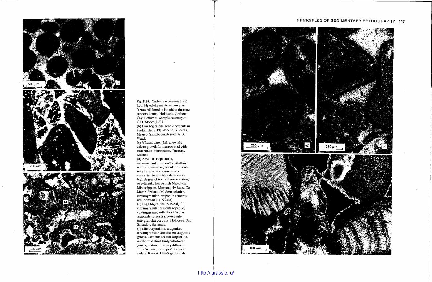
Fig. 5.30. Carbonate cements I: (a) Low Mg calcite meniscus cements (arrowed) forming in ooid grainstone subaerial dune. Holocene, Joulters Cay, Bahamas. Sample courtesy of C.H. Moore, LSU. (b) Low Mg calcite needle cements in aeolian dune. Pleistocene, Yucatan, Mexico. Sample courtesy of W.B. Ward. (c) Microcodium (M), a low Mg calcite growth form associated with root zones. Pleistocene, Yucatan, Mexico. (d) Acicular, isopachous, circumgranular cements in shallow marine grainstone; acicular cements may have been aragonite, since converted to low Mg calcite with a high degree of textural preservation, or originally low or high Mg calcite. Mississippian, Moyvoughly Beds, Co. Meath, Ireland. Modern acicular, circumgranular, aragonite cements are shown.in Fig. 5.24(a). (e) High Mg calcite, peloidal, circumgranular cements (opaque) coating grains, with later acicular aragonite cements growing into intergranular porosity. Holocene, San Salvador, Bahamas. (f) Microcrystalline, aragonite, circumgranular cements on aragonite grains. Cements are not isopachous and form distinct bridges between grains; textures are very different from 'micrite envelopes'. Crossed polars. Recent, US Virgin Islands.
http://jurassic.ru/
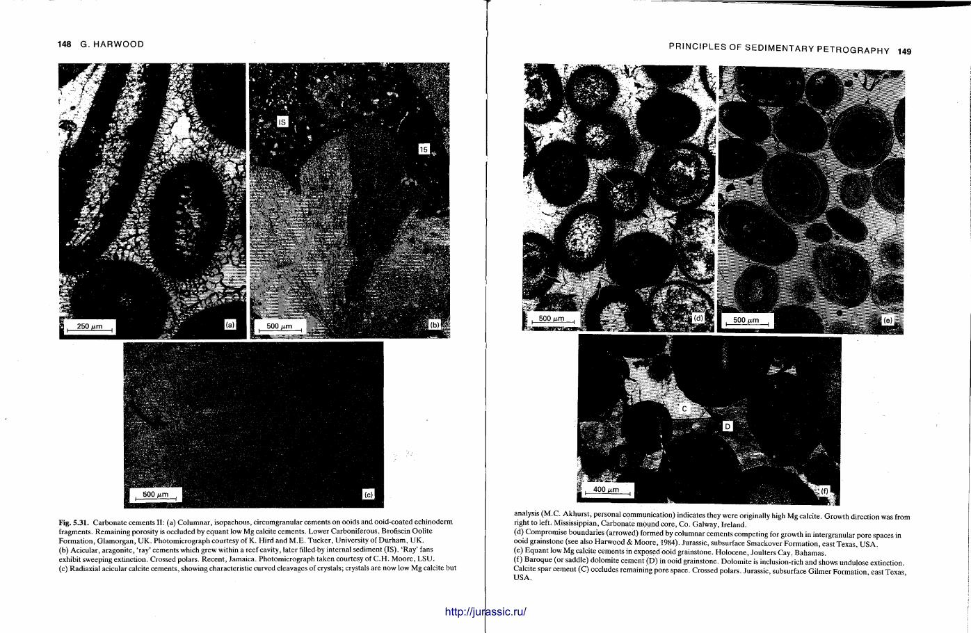
148 G. HARWOOD
Fig. 5 .31. Carbonate cements II: (a) Columnar, isopachous, circumgranular cements on ooids and ooid-coated echinoderm fragments. Remaining porosity is occluded by equant low Mg calcite cements. Lower Carboniferous, Brofiscin Oolite Formation, Glamorgan, UK. Photomicrograph courtesy of K. Hird and M.E. Tucker, University of Durham, UK. (b) Acicular, aragonite, 'ray' cements which grew within a reef cavity, later filled by internal sediment (IS). 'Ray' fans exhibit sweeping extinction. Crossed polars. Recent, Jamaica. Photomicrograph taken courtesy of C.H. Moore, LSU. (c) Radiaxial acicular calcite cements, showing characteristic curved cleavages of crystals; crystals are now low Mg calcite but
PRINCIPLES OF SEDIMENTARY PETROGRAPHY 149
analysis (M.C. Akhurst, personal communication) indicates they were originally high Mg calcite. Growth direction was from right to left; Mississippian, Carbonate mound core, Co. Galway, Ireland. (d) Compromise boundaries (arrowed) formed by columnar cements competing for growth in intergranular pore spaces in ooid grainstone (see also Harwood & Moore, 1984). Jurassic, subsurface Smackover Formation, east Texas, USA. (e) Equant low Mg calcite cements in exposed ooid grainstone. Holocene, Joulters Cay, Bahamas. (f) Baroque (or saddle) dolomite cement (D) in ooid grainstone. Dolomite is inclusion-rich and shows undulose extinction. Calcite spar cement (C) occludes remaining pore space. Crossed polars. Jurassic, subsurface Gilmer Formation, east Texas, USA.
http://jurassic.ru/
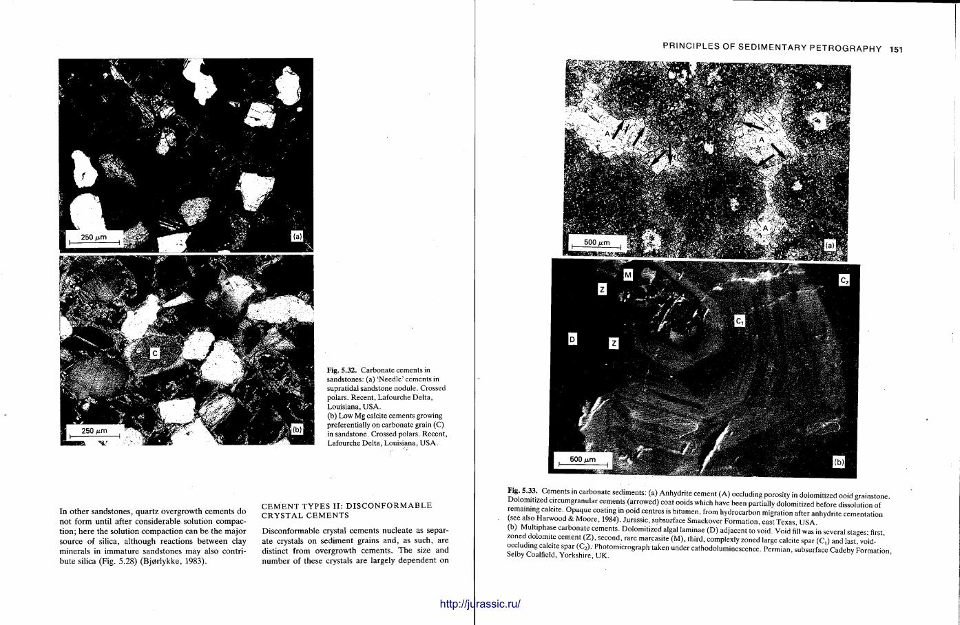
Fig. 5.32. Carbonate cements in sandstones: (a) 'Needle' cements in supratidal sandstone nodule. Crossed polars. Recent, Lafourche Delta, Louisiana, USA. (b) Low Mg calcite cements growing preferentially on carbonate grain (C) in sandstone. Crossed polars. Recent, Lafourche Delta, Louisiana, USA.
In other sandstones, quar tz overgrowth cements do not form until after considerable solution compaction; here the solution compaction can be the major source of silica, al though reactions between clay minerals in immature sandstones may also contribute silica (Fig. 5.28) (Bj0rlykke, 1983).
C E M E N T T Y P E S I I : D I S C O N F O R M A B L E C R Y S T A L C E M E N T S
Disconformable crystal cements nucleate as separate crystals on sediment grains and, as such, are distinct from overgrowth cements . T h e size and number of these crystals are largely dependent on
PRINCIPLES OF SEDIMENTARY PETROGRAPHY 151
Fig. 5.33. Cements in carbonate sediments: (a) Anhydrite cement (A) occluding porosity in dolomitized ooid grainstone. Dolomitized circumgranular cements (arrowed) coat ooids which have been partially dolomitized before dissolution of remaining calcite. Opaque coating in ooid centres is bitumen, from hydrocarbon migration after anhydrite cementation (see also Harwood & Moore, 1984). Jurassic, subsurface Smackover Formation, east Texas, USA. (b) Multiphase carbonate cements. Dolomitized algal laminae (D) adjacent to void. Void fill was in several stages; first, zoned dolomite cement (Z), second, rare marcasite (M), third, complexly zoned large calcite spar (C|) and last, void-occluding calcite spar (C 2). Photomicrograph taken under cathodoluminescence. Permian, subsurface Cadeby Formation, Selby Coalfield, Yorkshire, UK.
http://jurassic.ru/

152 G. H A R W O O D
the composit ion of the enclosing pore fluids and on the availability of the substrate to provide nucleation sites. Thus circumgranular (or rim) cements (Fig. 5.24a) form where there are many nucleation sites on a sediment grain, whereas poikilotopic cements (Fig. 5.24b) are the result of few nucleation sites and, in general , slower crystal growth. Characterization of the diverse morphologies of cements formed in modern diagenetic environments of rapid cementat ion has aided recognition of ancient analogues, particularly for near-surface carbonate diagenetic environments (for summaries see Longman, 1980; James & Choque t t e , 1983, 1984; Harr is , Kendall & Lerche , 1985). These , plus the carbonate cements formed during burial diagenesis are summarized in Fig. 5.29 with examples in Figs 5.30, 5.31 and 5.32; relevant additional comments on these diagenetic environments are included below.
V A D O S E A N D S H A L L O W M A R I N E C A R B O N A T E C E M E N T S
Although the cement morphologies summarized in Fig. 5.29 occur principally in carbonate sediments , quartz meniscus cements have been described from sandstones (e.g. Scholle, 1979, p . 114) and may comprise partial overgrowth cements . Near-surface carbonate cements also occur in quartzose sandstones but do not , however , form so readily on quartz grains (Fig. 5.30b, c) . This may be partly a factor of reduced possible nucleation sites and partly a result of the decreased supply of calcium carbonate . Siliciclastic sediments in general remain almost uncemented until buried to depths of 1000 m or more , whereas carbonate sediments are commonly cemented at or near the sediment—water interface, or in subaerial environments . Indirect evidence of vadose diagenesis in carbonates comes from 'fitted-textures ' (Fig. 5.16e), where expansion and or dissolution around grain margins has occurred beneath a soil zone.
A note of caution needs to be added concerning cementat ion in the meteoric vadose zone. Al though there is an ever-increasing li terature on cement morphologies and diagenesis within this zone , especially within soils, it is important to r emember that many such cements are the exception ra ther than the rule . In many modern examples, diagenetic reactions in the meteoric zones are minimal. Both modern and ancient zones show intense reaction within a few centimetres of the soil surface, perhaps
the area with least preservation potent ial , but very little alteration of the original sediment below that depth . Thus the presence of many ancient meteor ic vadose zones may be difficult to de termine from petrographic evidence and from field/core or geo-chemical techniques.
A further complication arises as many ancient shallow marine carbonate cements were of different mineralogies to those occurring in modern carbonates (e.g. Figs 5.24a, 5.30d, 5.31b, c) . However , al though the mineralogies may differ, the cement morphologies are commonly similar, thus enabling interpretat ion of ancient early diagenetic environments .
B U R I A L C E M E N T S
Carbonate burial cements are commonly coarsely crystalline, and include baroque dolomite and calcite spar (Fig. 5.31f), in places zoned. Burial cements in o ther sediments are composed of a complex range of mineralogies, not all of which are readily distinguishable with a petrological microscope (Table 5.1). Some are finely crystalline (clay minerals , hemat i te , l imonite) , others are coarsely crystalline (similar to carbonate burial cements) and commonly poikilotopic, whereas yet others are both coarsely crystalline and, to some extent , appear to replace the host sediment (anhydri te , halite, phosphates , glauconite) (Fig. 5.33a). Quar tz overgrowth cements are a further common burial cement , al though their presence alone is not an indication of deep burial . In siliciclastic sediments careful at tention to petrographic detail , particularly the compact ion history, is necessary to determine whether a cement formed during deep burial (>2 ,000 m) or at an earlier stage in the diagenetic history.
A t whatever stage in the diagenetic history of the sediment they form, cements are a record of the fluctuating pore water history of a sediment . Numerous , clearly identifiable stages of cementat ion in a sediment are evidence of changes in pore water chemistry and saturation states, even if all the precipitated phases are of a single mineralogy (e.g. Fig. 5.33b). More important , perhaps , is the evidence given by the termination of precipitation of a cement phase , indicating a decrease in saturat ion, or super-saturat ion, of that phase within the pore fluid and, in places, dissolution of pre-existing cement phases when undersa tura ted pore fluids are introduced into a sediment. Analysis of the chemistry and isotopic composit ions of the various cement phases can give
mmiHiiHiiiiiiiiiHiiiiiiii
P R I N C I P L E S OF S E D I M E N T A R Y P E T R O G R A P H Y 153
c HI
E
01 "D O
O C
a> e o
"D C
o o 0
r
o a
0
&
>• c/5
o a
-o
o -P ".p ° O CO ca a.— E o c_>
r
s
o •a
c r l - S CD i C
E ° X- I <" Q-Ico
OA
E
http://jurassic.ru/
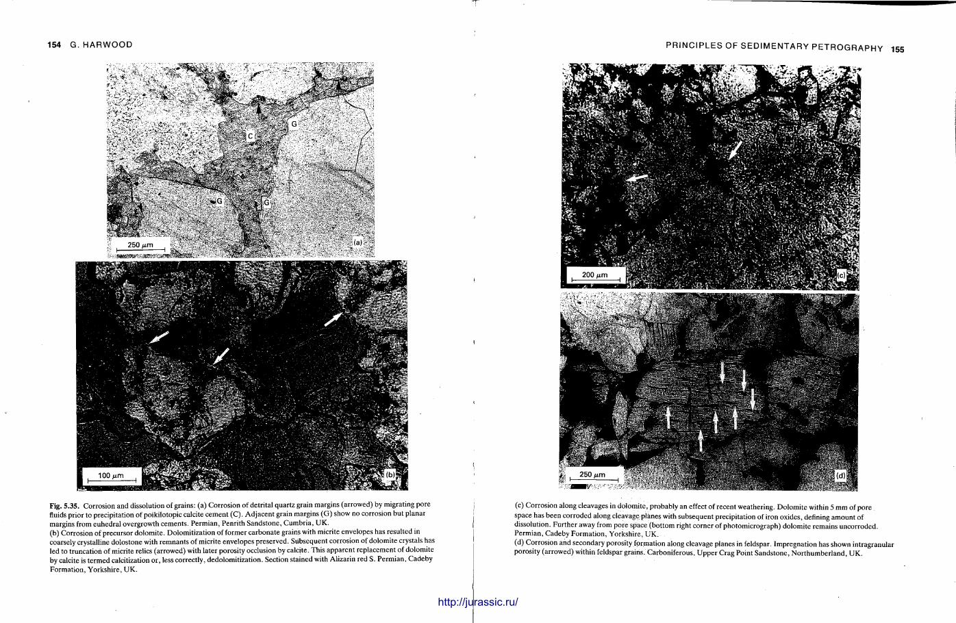
154 G. HARWOOD
Fig. 5.35. Corrosion and dissolution of grains: (a) Corrosion of detrital quartz grain margins (arrowed) by migrating pore fluids prior to precipitation of poikilotopic calcite cement (C). Adjacent grain margins (G) show no corrosion but planar margins from euhedral overgrowth cements. Permian, Penrith Sandstone, Cumbria, UK. (b) Corrosion of precursor dolomite. Dolomitization of former carbonate grains with micrite envelopes has resulted in coarsely crystalline dolostone with remnants of micrite envelopes preserved. Subsequent corrosion of dolomite crystals has led to truncation of micrite relics (arrowed) with later porosity occlusion by calcite. This apparent replacement of dolomite by calcite is termed calcitization or, less correctly, dedolomitization. Section stained with Alizarin red S. Permian, Cadeby Formation, Yorkshire, UK.
PRINCIPLES OF SEDIMENTARY PETROGRAPHY
(c) Corrosion along cleavages in dolomite, probably an effect of recent weathering. Dolomite within 5 mm of pore space has been corroded along cleavage planes with subsequent precipitation of iron oxides, defining amount of dissolution. Further away from pore space (bottom right corner of photomicrograph) dolomite remains uncorroded. Permian, Cadeby Formation, Yorkshire, UK. (d) Corrosion and secondary porosity formation along cleavage planes in feldspar. Impregnation has shown intragranular porosity (arrowed) within feldspar grains Carboniferous, Upper Crag Point Sandstone, Northumberland, UK.
http://jurassic.ru/
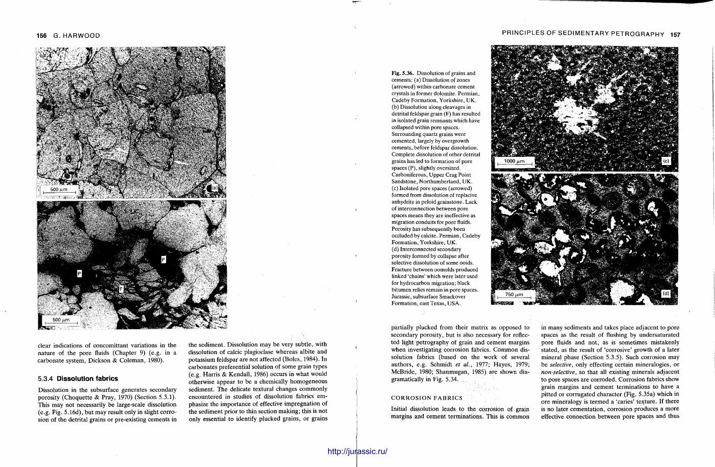
156 G. HARWOOD
clear indications of concomit tant variations in the na ture of the pore fluids (Chapter 9) (e.g. in a carbonate system, Dickson & Coleman , 1980).
5.3.4 Dissolut ion fabrics
Dissolution in the subsurface generates secondary porosity (Choquet te & Pray, 1970) (Section 5.3.1). This may not necessarily b e large-scale dissolution (e.g. Fig. 5.16d), but may result only in slight corrosion of the detrital grains or pre-existing cements in
the sediment. Dissolution may be very subtle, with dissolution of calcic plagioclase whereas albite and potassium feldspar are not affected (Boles, 1984). In carbonates preferential solution of some grain types (e.g. Harr is & Kendal l , 1986) occurs in what would otherwise appear t o be a chemically homogeneous sediment. The delicate textural changes commonly encountered in studies of dissolution fabrics emphasize the impor tance of effective impregnat ion of the sediment prior to thin section making; this is no t only essential to identify plucked grains, or grains
PRINCIPLES OF SEDIMENTARY PETROGRAPHY 157
Fig. 5.36. Dissolution of grains and cements: (a) Dissolution of zones (arrowed) within carbonate cement crystals in former dolomite. Permian, Cadeby Formation, Yorkshire, UK. (b) Dissolution along cleavages in detrital feldspar grain (F) has resulted in isolated grain remnants which have collapsed within pore spaces. Surrounding quartz grains were cemented, largely by overgrowth cements, before feldspar dissolution. Complete dissolution of other detrital grains has led to formation of pore spaces (P), slightly oversized. Carboniferous, Upper Crag Point Sandstone, Northumberland, UK. (c) Isolated pore spaces (arrowed) formed from dissolution of replacive anhydrite in peloid grainstone. Lack of interconnection between pore spaces means they are ineffective as migration conduits for pore fluids. Porosity has subsequently been occluded by calcite. Permian, Cadeby Formation, Yorkshire, UK. (d) Interconnected secondary porosity formed by collapse after selective dissolution of some ooids. Fracture between oomolds produced linked 'chains' which were later used for hydrocarbon migration; black bitumen relics remain in pore spaces. Jurassic, subsurface Smackover Formation, east Texas, USA.
partially plucked from their matrix as opposed to secondary porosity, but is also necessary for reflected light pet rography of grain and cement margins when investigating corrosion fabrics. C o m m o n dissolution fabrics (based on the work of several authors , e.g. Schmidt et al., 1977; Hayes , 1979; McBride , 1980; Shanmugan, 1985) are shown dia-gramatically in Fig. 5.34.
C O R R O S I O N F A B R I C S
Initial dissolution leads to the corrosion of grain margins and cement te rminat ions . This is common
in many sediments and takes place adjacent to pore spaces as the result of flushing by undersaturated pore fluids and not , as is sometimes mistakenly stated, as the result of 'corrosive' growth of a later mineral phase (Section 5.3.5). Such corrosion may be selective, only effecting certain mineralogies, or non-selective, so that all existing minerals adjacent to pore spaces are corroded. Corrosion fabrics show grain margins and cement terminations to have a pit ted or corrugated character (Fig. 5.35a) which in ore mineralogy is te rmed a 'caries' texture. If there is no later cementat ion, corrosion produces a more effective connection be tween pore spaces and thus
http://jurassic.ru/
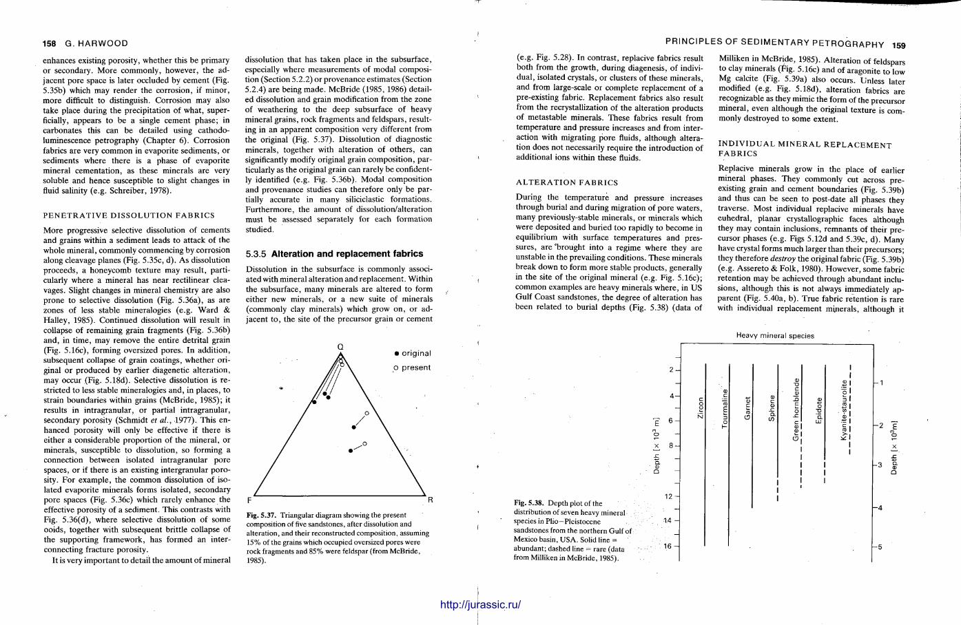
158 G. HARWOOD
dissolution that has taken place in the subsurface, especially where measurements of modal composition (Section 5.2.2) or provenance estimates (Section 5.2.4) are being made . McBride (1985, 1986) detailed dissolution and grain modification from the zone of weathering to the deep subsurface of heavy mineral grains, rock fragments and feldspars, resulting in an apparent composition very different from the original (Fig. 5.37). Dissolution of diagnostic minerals , together with alteration of o thers , can significantly modify original grain composit ion, particularly as the original grain can rarely be confidently identified (e.g. Fig. 5.36b). Modal composit ion and provenance studies can therefore only be partially accurate in many siliciclastic formations. Fur the rmore , the amount of dissolution/alteration must be assessed separately for each formation studied.
5.3.5 Alteration and replacement fabr ics
Dissolution in the subsurface is commonly associated with mineral alteration and replacement . Within the subsurface, many minerals are altered to form either new minerals , or a new suite of minerals (commonly clay minerals) which grow on , or adjacent t o , the site of the precursor grain or cement
F R
Fig. 5.37. Triangular diagram showing the present composition of five sandstones, after dissolution and alteration, and their reconstructed composition, assuming 15% of the grains which occupied oversized pores were rock fragments and 85% were feldspar (from McBride, 1985).
(e.g. Fig. 5.28). In contrast , replacive fabrics result both from the growth, during diagenesis, of individual , isolated crystals, or clusters of these minerals , and from large-scale or complete replacement of a pre-existing fabric. Replacement fabrics also result from the recrystallization of the alteration products of metastable minerals. These fabrics result from tempera ture and pressure increases and from interaction with migrating pore fluids, al though alteration does not necessarily require the introduction of additional ions within these fluids.
A L T E R A T I O N F A B R I C S
Dur ing the t empera tu re and pressure increases through burial and during migration of pore waters , many previously-stable minerals , or minerals which were deposi ted and bur ied too rapidly to become in equilibrium with surface tempera tures and pressures, are "brought into a regime where they are unstable in the prevailing condit ions. These minerals break down to form more stable products , generally in the site of the original mineral (e.g. Fig. 5.16c); common examples are heavy minerals where , in US Gulf Coast sandstones, the degree of alteration has been related to burial depths (Fig. 5.38) (data of
PRINCIPLES OF SEDIMENTARY PETROGRAPHY 159
Fig. 5.38. Depth plot of the distribution of seven heavy mineral species in Plio-Pleistocene sandstones from the northern Gulf of Mexico basin, USA. Solid line = abundant; dashed line = rare (data from Milliken in McBride, 1985).
4H
c1 6-
D.
12 H
••1.4 H
16 H
Heavy mineral species
CD
CD
CO . i E . > .
Q. CD Q
1111
Milliken in McBride , 1985). Alterat ion of feldspars to clay minerals (Fig. 5.16c) and of aragonite t o low Mg calcite (Fig. 5.39a) also occurs. Unless later modified (e.g. Fig. 5.18d), alteration fabrics are recognizable as they mimic the form of the precursor mineral , even although the original texture is commonly destroyed to some extent .
I N D I V I D U A L M I N E R A L R E P L A C E M E N T F A B R I C S
Replacive minerals grow in the place of earlier mineral phases. They commonly cut across preexisting grain and cement boundaries (Fig. 5.39b) and thus can b e seen to post-date all phases they traverse. Most individual replacive minerals have euhedra l , planar crystallographic faces although they may contain inclusions, remnants of their precursor phases (e .g. Figs 5.12d and 5.39c, d) . Many have crystal forms much larger than their precursors; they therefore destroy the original fabric (Fig. 5.39b) (e.g. Assereto & Folk, 1980). However , some fabric re tent ion may b e achieved through abundant inclusions, al though this is not always immediately apparent (Fig. 5.40a, b) . T rue fabric retention is rare with individual replacement minerals , al though it
enhances existing porosity, whether this be primary or secondary. More commonly, however , the adjacent pore space is later occluded by cement (Fig. 5.35b) which may render the corrosion, if minor , more difficult to distinguish. Corrosion may also take place during the precipitation of what , superficially, appears to be a single cement phase; in carbonates this can be detailed using ca thodoluminescence petrography (Chapter 6). Corrosion fabrics are very common in evaporite sediments , or sediments where there is a phase of evapori te mineral cementat ion, as these minerals are very soluble and hence susceptible to slight changes in fluid salinity (e.g. Schreiber, 1978).
P E N E T R A T I V E D I S S O L U T I O N F A B R I C S
More progressive selective dissolution of cements and grains within a sediment leads to attack of the whole mineral , commonly commencing by corrosion along cleavage planes (Fig. 5.35c, d) . As dissolution proceeds , a honeycomb texture may result , part icularly where a mineral has near rectilinear cleavages. Slight changes in mineral chemistry are also p rone to selective dissolution (Fig. 5.36a), as are zones of less stable mineralogies (e.g. Ward & Halley, 1985). Cont inued dissolution will result in collapse of remaining grain fragments (Fig. 5.36b) and, in t ime, may remove the entire detrital grain (Fig. 5.16c), forming oversized pores. In addit ion, subsequent collapse of grain coatings, whether original or produced by earlier diagenetic al terat ion, may occur (Fig. 5.18d). Selective dissolution is restricted to less stable mineralogies and, in places, to strain boundaries within grains (McBride, 1985); it results in intragranular , or partial intragranular , secondary porosity (Schmidt et al., 1977). This enhanced porosity will only be effective if there is either a considerable propor t ion of the mineral , or minerals , susceptible to dissolution, so forming a connection be tween isolated intragranular pore spaces, or if there is an existing intergranular porosity. For example , the common dissolution of isolated evaporite minerals forms isolated, secondary pore spaces (Fig. 5.36c) which rarely enhance the effective porosity of a sediment. This contrasts with Fig. 5.36(d), where selective dissolution of some ooids, together with subsequent brittle collapse of the supporting framework, has formed an interconnecting fracture porosity.
It is very important to detail the amount of mineral
http://jurassic.ru/
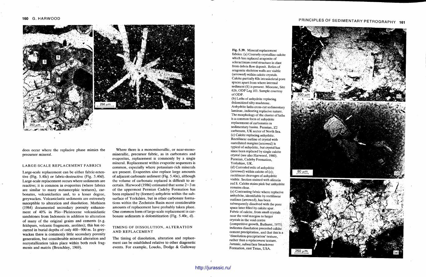
160 G. HARWOOD
does occur where the replacive phase mimics the precursor mineral .
L A R G E - S C A L E R E P L A C E M E N T F A B R I C S
Large-scale replacement can be either fabric-retentive (Fig. 5.40c) or fabric-destructive (Fig. 5.40d). Large-scale replacement occurs where sediments are reactive; it is common in evaporites (where fabrics are similar to many metamorphic textures) , carbonates , volcaniclastics and, to a lesser degree , greywackes. Volcaniclastic sediments are extremely susceptible to alteration and dissolution. Mathisen (1984) documented secondary porosity enhancement of 4 0 % in P l io -P le i s tocene volcaniclastic sandstones from Indonesia in addition to alteration of many of the original grains and cements (e.g. feldspars, volcanic fragments, zeolites); this has occurred in burial depths of only 4 0 0 - 9 0 0 m. In greywackes there is commonly little secondary porosity generat ion, but considerable mineral alteration and recrystallization takes place within both rock fragments and matrix (Brenchley, 1969).
Where there is a monomineral l ic , or nea r -mono-minerallic, precursor fabric, as in carbonates and evapori tes, replacement is commonly by a single mineral . Replacement within evapori te sequences is common, especially where potassium-rich minerals are present . Evapori tes also replace large amounts of adjacent carbonate sediment (Fig. 5.40e), although the volume of carbonate replaced is difficult to ascertain. Harwood (1986) estimated that some 2—3 m of the uppermost Permian Cadeby Format ion has been replaced by (former) anhydri te within the subsurface of Yorkshi re , but in o ther carbonate formations within the Zechstein Basin more considerable amounts of replacement have probably taken place. O n e common form of large-scale replacement in carbonate sediments is dolomitization (Fig. 5.40c, d ) .
T I M I N G O F D I S S O L U T I O N , A L T E R A T I O N A N D R E P L A C E M E N T
The timing of dissolution, al teration and replacement can be established relative to o ther diagenetic events . For example , Loucks , Dodge & Galloway
PRINCIPLES OF SEDIMENTARY PETROGRAPHY 161
Fig, 5.39. Mineral replacement fabrics: (a) Coarsely crystalline calcite which has replaced aragonite of scleractinian coral structure in clast from debris flow deposit. Relics of aragonite skeleton walls are visible (arrowed) within calcite crystals. Calcite partially fills intraskeletal pore spaces apart from where internal sediment (S) is present. Miocene, Site 626, ODP Leg 10i. Sample courtesy of ODP. (b) Laths of anhydrite replacing dolomitized silty mudstone. Anhydrite laths cross-cut sedimentary laminae, indicating replacive nature. The morphology of the cluster of laths is a common form of anhydrite replacement of carbonates in sedimentary basins. Permian, Z2 carbonate, UK sector of North Sea. (c) Calcite replacing anhydrite. Rectilinear outline of crystal with castellated margins (arrowed) is typical of anhydrite, but crystal has since been replaced by single calcite crystal (see also Harwood, 1980). Permian, Cadeby Formation, Yorkshire, UK. (d) Corroded relic of anhydrite (arrowed) within calcite of (c); rectilinear cleavages of anhydrite visible. Section stained with alizarin red S. Calcite stains pink but anhydrite remains clear. (e) Contrasting fabric where replacive anhydrite, identifiable by rectilinear outlines (arrowed), has been subsequently dissolved with the pore space later filled by calcite spar. Fabric of calcite, from small crystals near the void margins to larger crystals in the void centre (competitive growth, Bathurst, 1975) indicates dissolution preceded calcite cement precipitation, and that this is a 'dissolution-precipitation' texture, rather than a replacement texture. Jurassic, subsurface Smackover Formation, east Texas, USA.
http://jurassic.ru/
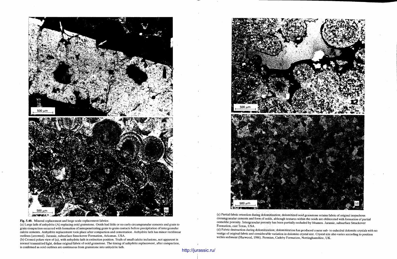
Fig. 5.40. Mineral replacement and large-scale replacement fabrics: (a) Large lath of anhydrite (A) replacing ooid grainstone. Ooids had little or no early circumgranular cements and grain to grain compaction occurred with formation of interpenetrating grain to grain contacts before precipitation of intergranular calcite cements. Anhydrite replacement took place after compaction and cementation. Anhydrite lath has minor rectilinear outlines (arrowed). Jurassic, subsurface Smackover Formation, Arkansas, USA. (b) Crossed polars view of (a), with anhydrite lath in extinction position. Trails of small calcite inclusions, not apparent in normal transmitted light, define original fabric of ooid grainstone. The timing of anhydrite replacement, after compaction, is confirmed as ooid outlines are continuous from grainstone into anhydrite lath.
Bitlillill
(c) Partial fabric retention during doldmitization; dolomitized ooid grainstone retains fabric of original isopachous circumgranular cements and form of ooids. although textures within the ooids are obliterated with formation of partial oomoldic porosity. Intergranular porosity has been partially occluded by bitumen. Jurassic, subsurface Smackover Formation, east Texas, USA. (d) Fabric destruction during dolomitization; dolomitization has produced coarse sub- to euhedral dolomite crystals with vestige of original fabric and considerable variation in dolomite crystal size. Crystal size also varies according to position within sediment (Harwood, 1986). Permian, Cadeby Formation, Nottinghamshire, UK.
http://jurassic.ru/
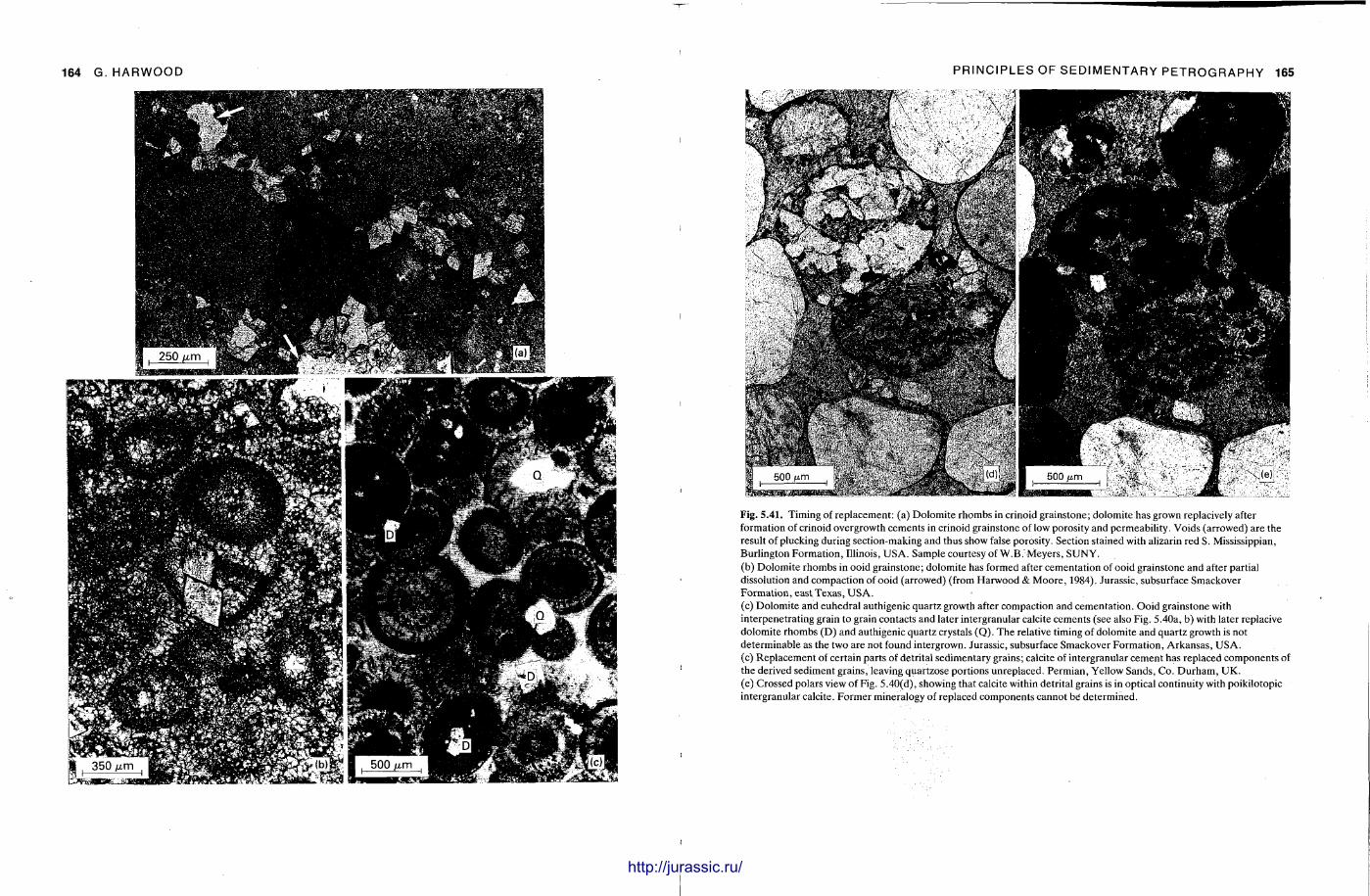
I
PRINCIPLES OF SEDIMENTARY PETROGRAPHY 165
Fig. 5 .41. Timing of replacement: (a) Dolomite rhombs in crinoid grainstone; dolomite has grown replacively after formation of crinoid overgrowth cements in crinoid grainstone of low porosity and permeability. Voids (arrowed) are the result of plucking during section-making and thus show false porosity. Section stained with alizarin red S. Mississippian, Burlington Formation, Illinois, USA. Sample courtesy of W.B. Meyers, SUNY. (b) Dolomite rhombs in ooid grainstone; dolomite has formed after cementation of ooid grainstone and after partial dissolution and compaction of ooid (arrowed) (from Harwood & Moore, 1984). Jurassic, subsurface Smackover Formation, east Texas, USA. (c) Dolomite and euhedral authigenic quartz growth after compaction and cementation. Ooid grainstone with interpenetrating grain to grain contacts and later intergranular calcite cements (see also Fig. 5.40a, b) with later replacive dolomite rhombs (D) and authigenic quartz crystals (Q). The relative timing of dolomite and quartz growth is not determinable as the two are not found intergrown. Jurassic, subsurface Smackover Formation, Arkansas, USA. (c) Replacement of certain parts of detrital sedimentary grains; calcite of intergranular cement has replaced components of the derived sediment grains, leaving quartzose portions unreplaced. Permian, Yellow Sands, Co. Durham, UK. (e) Crossed polars view of Fig. 5.40(d), showing that calcite within detrital grains is in optical continuity with poikilotopic intergranular calcite. Former mineralogy of replaced components cannot be determined.
http://jurassic.ru/
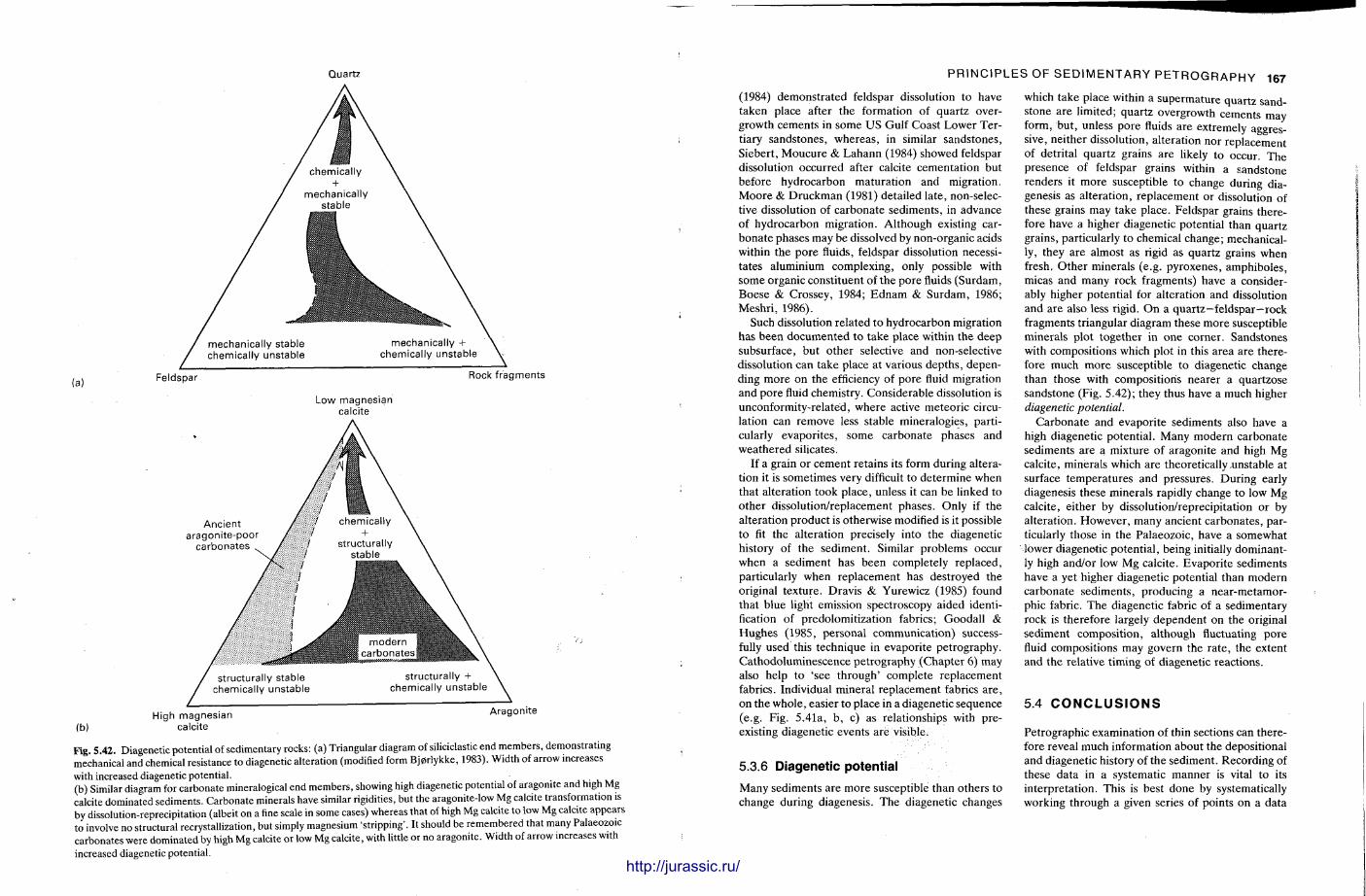
Quartz
Fig. 5.42. Diagenetic potential of sedimentary rocks: (a) Triangular diagram of siliciclastic end members, demonstrating mechanical and chemical resistance to diagenetic alteration (modified form Bj0rlykke, 1983). Width of arrow increases with increased diagenetic potential. (b) Similar diagram for carbonate mineralogical end members, showing high diagenetic potential of aragonite and high Mg calcite dominated sediments. Carbonate minerals have similar rigidities, but the aragonite-low Mg calcite transformation is by dissolution-reprecipitation (albeit on a fine scale in some cases) whereas that of high Mg calcite to low Mg calcite appears to involve no structural recrystallization, but simply magnesium 'stripping'. It should be remembered that many Palaeozoic carbonates were dominated by high Mg calcite or low Mg calcite, with little or no aragonite. Width of arrow increases with increased diagenetic potential.
PRINCIPLES OF SEDIMENTARY PETROGRAPHY
(1984) demonst ra ted feldspar dissolution to have taken place after the formation of quartz overgrowth cements in some US Gulf Coast Lower Tertiary sandstones, whereas , in similar sandstones, Siebert , Moucure & Lahann (1984) showed feldspar dissolution occurred after calcite cementat ion but before hydrocarbon maturat ion and migration. Moore & Druckman (1981) detailed late, non-selective dissolution of carbonate sediments , in advance of hydrocarbon migration. Al though existing carbonate phases may be dissolved by non-organic acids within the pore fluids, feldspar dissolution necessitates aluminium complexing, only possible with some organic constituent of the pore fluids (Surdam, Boese & Crossey, 1984; E d n a m & Surdam, 1986; Meshr i , 1986).
Such dissolution related to hydrocarbon migration has been documented to t ake place within the deep subsurface, but other selective and non-selective dissolution can take place at various depths , depending more on the efficiency of pore fluid migration and pore fluid chemistry. Considerable dissolution is unconformity-related, where active meteoric circulation can remove less stable mineralogies, part icularly evapori tes, some carbonate phases and weathered silicates.
If a grain or cement retains its form during alteration it is sometimes very difficult to determine when that alteration took place, unless it can be linked to other dissolution/replacement phases. Only if the alteration product is otherwise modified is it possible to fit the alteration precisely into the diagenetic history of the sediment. Similar problems occur when a sediment has been completely replaced, particularly when replacement has destroyed the original texture. Dravis & Yurewicz (1985) found that blue light emission spectroscopy aided identification of predolomitizat ion fabrics; Goodall & Hughes (1985, personal communicat ion) successfully used this technique in evaporite petrography. Cathodoluminescence petrography (Chapter 6) may also help to 'see through ' complete replacement fabrics. Individual mineral replacement fabrics a re , on the whole , easier to place in a diagenetic sequence (e.g. Fig. 5.41a, b , c) as relationships with preexisting diagenetic events are visible.
5.3.6 Diagenetic potential
Many sediments are more susceptible than others to change during diagenesis. The diagenetic changes
which take place within a supermature quartz sandstone are limited; quartz overgrowth cements may form, but , unless pore fluids are extremely aggressive, nei ther dissolution, alteration nor replacement of detrital quartz grains are likely to occur. The presence of feldspar grains within a sandstone renders it more susceptible to change during diagenesis as al terat ion, replacement or dissolution of these grains may take place. Feldspar grains therefore have a higher diagenetic potential than quartz grains, particularly to chemical change; mechanically, they are almost as rigid as quartz grains when fresh. Other minerals (e.g. pyroxenes, amphiboles, micas and many rock fragments) have a considerably higher potential for alteration and dissolution and are also less rigid. O n a quartz—feldspar—rock fragments triangular diagram these more susceptible minerals plot together in one corner. Sandstones with compositions which plot in this area are therefore much more susceptible to diagenetic change than those with composit ions nearer a quartzose sandstone (Fig. 5.42); they thus have a much higher diagenetic potential.
Carbona te and evaporite sediments also have a high diagenetic potent ial . Many modern carbonate sediments are a mixture of aragonite and high Mg calcite, minerals which are theoretically .unstable at surface tempera tures and pressures. Dur ing early diagenesis these minerals rapidly change to low Mg calcite, either by dissolution/reprecipitation or by alteration. However , many ancient carbonates , particularly those in the Palaeozoic, have a somewhat lower diagenetic potential , being initially dominant-ly high and/or low Mg calcite. Evapor i te sediments have a yet higher diagenetic potential than modern carbonate sediments , producing a near-metamor-phic fabric. T h e diagenetic fabric of a sedimentary rock is therefore largely dependent on the original sediment composit ion, although fluctuating pore fluid compositions may govern the ra te , the extent and the relative t iming of diagenetic reactions.
5.4 C O N C L U S I O N S
Petrographic examination of thin sections can therefore reveal much information about the depositional and diagenetic history of the sediment. Recording of these data in a systematic manner is vital to its interpretat ion. This is best done by systematically working through a given series of points on a data
http://jurassic.ru/

168 G. HARWOOD
Sedimentary Petrography Petrographer Date
Description Form Specimen
Terr igenous s e d i m e n t s
Hand s p e c i m e n Colour: Fresh— Weathered
Structures:
Grain size: Max mm Min Roundness Models) Sphericity
Sorting: Other features:
Thin s e c t i o n
Apparent grain size: Max Roundness. Min Sphericity . Models) Sorting
Detrital composition % Quartz K feldspar Plagioclase Rock fragments Muscovite Biotite Heavy minerals Opaque minerals Carbonates Matrix Others
Diagenetic components Cement Other authigenic
minerals
Compaction (type and degree)
(a)
Quartz varieties:
monocrystalline < ^ ,
polycrystalline < ^
Matrix components:
Porosity: Type
Primary
Secondary
PRINCIPLES OF SEDIMENTARY PETROGRAPHY 1
Components on triangular diagrams
Allochemical Orthochemical Framework Cement
Diagenetic events
Sketch of key fabric(s)
Comments and interpretations
Fig. 5.43. Data sheets for systematically recording petrographic observations; sheet A is for terrigenous sediments and sheet B for carbonates. Sheets can be combined if all observational criteria are not itemized.
http://jurassic.ru/

170 G. HARWOOD
Sedimentary Petrography Petrographer ... Date ...
Description Form Specimen ...
C a r b o n a t e / e v a p o r i t e s e d i m e n t s
Hand s p e c i m e n Colour: Fresh Weathered .. Induration: „ x
Structures: Grain size: Max.
Min. Rock type (Durham class.) Mode(s) Skeletal clasts
Sorting: Other features
Thin s e c t i o n
Detrital grains Size Skeletal types ((im) Roundness Fragmentation
Intraclasts Ooids Pellets Peloids Quartz grains Feldspar grains Other detrital
minerals ...
Matrix Evaporites % Size Comments
Gypsum , Anhydrite Halite Others
(b)
PRINCIPLES OF SEDIMENTARY PETROGRAP
Other authigenic minerals
Compaction (type and degree)
Components on triangular diagrams
1. Origin of components 2. Fabric of components. 3. Three appropriate
Detrital A Matrix components
Allochemical Orthochemical Framework grains
(I = impure)
Cement
Diagenetic events
Sketch of key fabric(s)
Comments and interpretation
Diagenetic components Porosity
Cement type % Type
Primary
Secondary
http://jurassic.ru/
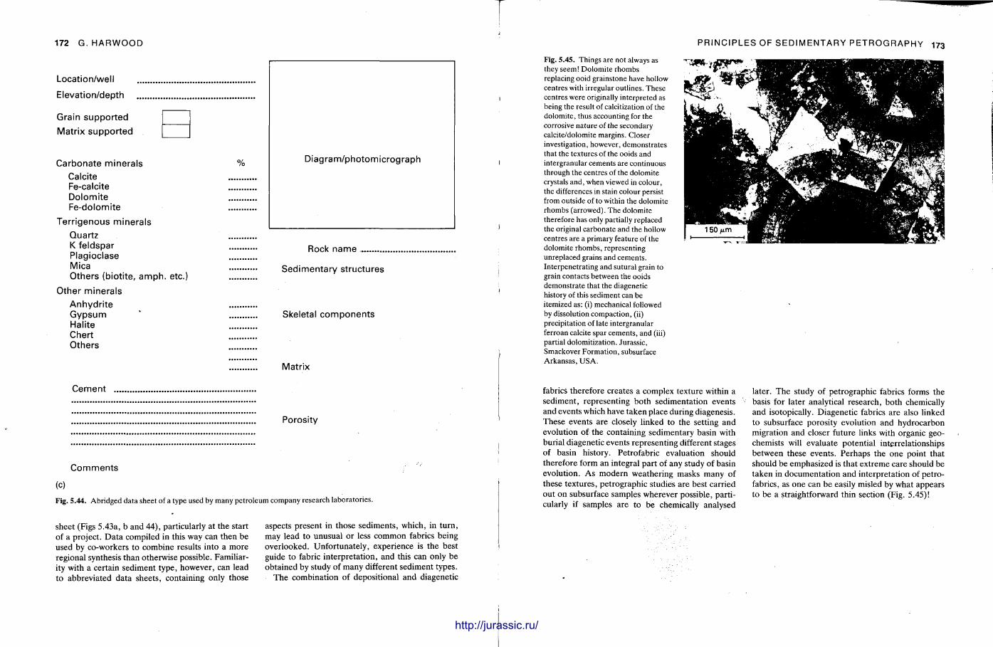
T 172 G. HARWOOD
Location/well
Elevation/depth
Grain supported Matrix supported
Carbonate minerals °/° Calcite Fe-calcite Dolomite Fe-dolomite
Terrigenous minerals Q u a r t z K feldspar Plagioclase Mica Others (biotite, amph. etc.)
Other minerals
Anhydri te Gypsum ' Halite C h e r t Others
Cement
Diagram/photomicrograph
Rock name „
Sedimentary structures
Skeletal components
Matrix
Porosity
Comments
(c)
Fig. 5 .44 . Abridged data sheet of a type used by many petroleum company research laboratories.
sheet (Figs 5.43a, b and 44), particularly at the start of a project. D a t a compiled in this way can then be used by co-workers to combine results into a more regional synthesis than otherwise possible. Familiarity with a certain sediment type, however , can lead to abbreviated data sheets , containing only those
aspects present in those sediments , which, in turn , may lead to unusual or less common fabrics being overlooked. Unfor tunately , experience is the best guide to fabric interpretat ion, and this can only be obtained by study of many different sediment types.
The combinat ion of depositional and diagenetic
n i l l
PRINCIPLES OF SEDIMENTARY PETROGRAPHY 173
Fig. 5 . 4 5 . Things are not always as they seem! Dolomite rhombs replacing ooid grainstone have hollow centres with irregular outlines. These centres were originally interpreted as being the result of calcitization of the dolomite, thus accounting for the corrosive nature of the secondary calcite/dolomite margins. Closer investigation, however, demonstrates that the textures of the ooids and intergranular cements are continuous through the centres of the dolomite crystals and, when viewed in colour, the differences in stain colour persist from outside of to within the dolomite rhombs (arrowed). The dolomite therefore has only partially replaced the original carbonate and the hollow centres are a primary feature of the dolomite rhombs, representing unreplaced grains and cements. Interpenetrating and sutural grain to grain contacts between the ooids demonstrate that the diagenetic history of this sediment can be itemized as: (i) mechanical followed by dissolution compaction, (ii) precipitation of late intergranular ferroan calcite spar cements, and (iii) partial dolomitization. Jurassic, Smackover Formation, subsurface Arkansas, USA.
fabrics therefore creates a complex texture within a sediment , representing bo th sedimentation events and events which have taken place during diagenesis. These events are closely linked to the setting and evolution of the containing sedimentary basin with burial diagenetic events representing different stages of basin history. Petrofabric evaluation should therefore form an integral part of any study of basin evolution. As modern weathering masks many of these textures , petrographic studies are best carried out on subsurface samples wherever possible, part icularly if samples are to be chemically analysed
later. The study of petrographic fabrics forms the basis for later analytical research, both chemically and isotopically. Diagenetic fabrics are also linked to subsurface porosity evolution and hydrocarbon migration and closer future links with organic geo-chemists will evaluate potential interrelationships between these events. Perhaps the one point that should be emphasized is that extreme care should be taken in documentat ion and interpretat ion of petrofabrics, as one can be easily misled by what appears to be a straightforward thin section (Fig. 5.45)!
http://jurassic.ru/
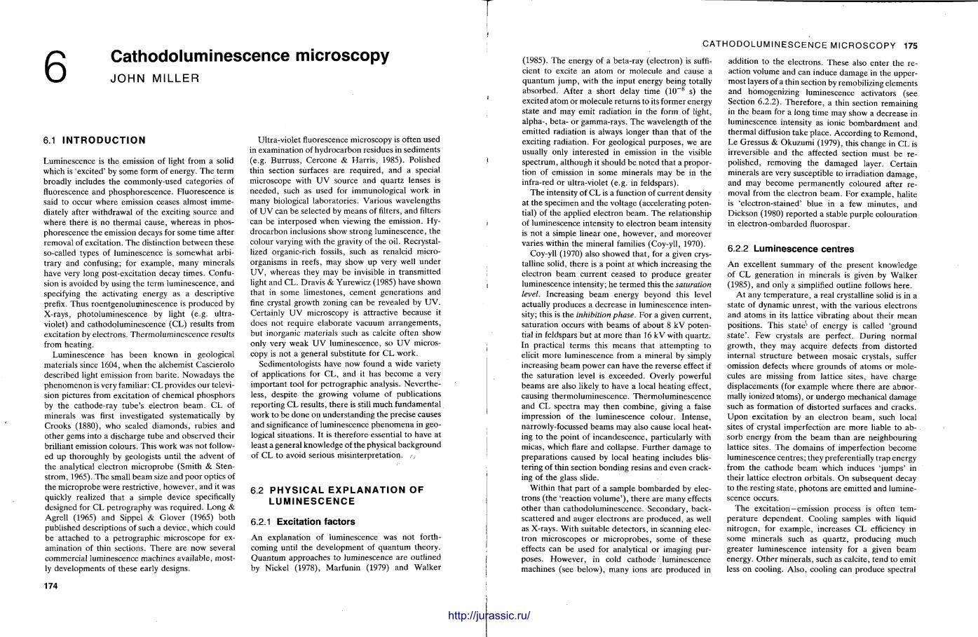
Cathodoluminescence microscopy JOHN MILLER
6.1 I N T R O D U C T I O N
Luminescence is the emission of light from a solid which is 'excited' by some form of energy. The term broadly includes the commonly-used categories of fluorescence and phosphorescence. Fluorescence is said to occur where emission ceases almost immediately after withdrawal of the exciting source and where there is no thermal cause, whereas in phosphorescence the emission decays for some t ime after removal of excitation. The distinction be tween these so-called types of luminescence is somewhat arbitrary and confusing; for example , many minerals have very long post-excitation decay t imes. Confusion is avoided by using the term luminescence, and specifying the activating energy as a descriptive prefix. Thus roentgenoluminescence is produced by X-rays, photoluminescence by light (e.g. ultraviolet) and cathodoluminescence (CL) results from excitation by electrons. Thermoluminescence results from heating.
Luminescence has been known in geological materials since 1604, when the alchemist Cascierolo described light emission from barite. Nowadays the phenomenon is very familiar: CL provides our television pictures from excitation of chemical phosphors by the cathode-ray tube 's electron beam. C L of minerals was first investigated systematically by Crooks (1880), who sealed d iamonds , rubies and other gems into a discharge tube and observed their brilliant emission colours. This work was not followed up thoroughly by geologists until the advent of the analytical electron microprobe (Smith & Sten-strom, 1965). The small beam size and poor optics of the microprobe were restrictive, however , and it was quickly realized that a simple device specifically designed for CL petrography was required. Long & Agrell (1965) and Sippel & Glover (1965) both published descriptions of such a device, which could be at tached to a petrographic microscope for examination of thin sections. There are now several commercial luminescence machines available, mostly developments of these early designs.
Ultra-violet fluorescence microscopy is often used in examination of hydrocarbon residues in sediments (e.g. Burruss , Cercone & Harr i s , 1985). Polished thin section surfaces are required, and a special microscope with U V source and quartz lenses is needed , such as used for immunological work in many biological laboratories . Various wavelengths of U V can be selected by means of filters, and filters can be interposed when viewing the emission. Hydrocarbon inclusions show strong luminescence, the colour varying with the gravity of the oil. Recrystallized organic-rich fossils, such as renalcid microorganisms in reefs, may show up very well under U V , whereas they may be invisible in t ransmit ted light and CL. Dravis & Yurewicz (1985) have shown that in some l imestones, cement generat ions and fine crystal growth zoning can be revealed by U V . Certainly U V microscopy is attractive because it does not require e laborate vacuum ar rangements , but inorganic materials such as calcite often show only very weak U V luminescence, so U V microscopy is not a general substitute for C L work.
Sedimentologists have now found a wide variety of applications for C L , and it has become a very important tool for petrographic analysis. Never theless, despite the growing volume of publications report ing CL results, there is still much fundamental work to be done on unders tanding the precise causes and significance of luminescence phenomena in geological situations. It is therefore-essential to have at least a general knowledge of the physical background of CL to avoid serious misinterpretat ion.
6.2 P H Y S I C A L E X P L A N A T I O N OF L U M I N E S C E N C E
6.2.1 Excitation factors
A n explanation of luminescence was not forthcoming until the development of quan tum theory. Quan tum approaches to luminescence are outlined by Nickel (1978), Marfunin (1979) and Walker
174
CATHODOLUMINESCENCE MICROSCOPY 175
(1985). The energy of a beta-ray (electron) is sufficient to excite an a tom or molecule and cause a quan tum j u m p , with the input energy being totally absorbed. After a short delay time ( 1 0 - 8 s) the
1 excited a tom or molecule re turns to its former energy state and may emit radiation in the form of light, alpha-, beta- or gamma-rays. T h e wavelength of the emitted radiation is always longer than that of the exciting radiat ion. For geological purposes , we are usually only interested in emission in the visible
1 spectrum, although it should be noted that a proportion of emission in some minerals may be in the infra-red or ultra-violet (e.g. in feldspars).
T h e intensity of CL is a function of current density at the specimen and the voltage (accelerating potential) of the applied electron beam. The relationship
i of luminescence intensity to electron beam intensity is not a simple linear one , however, and moreover varies within the mineral families (Coy-yll, 1970).
Coy-yll (1970) also showed that , for a given crystalline solid, there is a point at which increasing the electron beam current ceased to produce greater
i luminescence intensity; he te rmed this the saturation level. Increasing beam energy beyond this level actually produces a decrease in luminescence intensity; this is the inhibition phase. For a given current , saturation occurs with beams of about 8 kV potential in feldspars but at more than 16 k V with quartz .
j In practical terms this means that at tempting to elicit more luminescence from a mineral by simply increasing beam power can have the reverse effect if the saturation level is exceeded. Overly powerful beams are also likely to have a local heating effect, causing thermoluminescence. Thermoluminescence and CL spectra may then combine, giving a false impression of the luminescence colour. Intense, narrowly-focussed beams may also cause local heating to the point of incandescence, particularly with micas, which flare and collapse. Fur ther damage to preparat ions caused by local heating includes blistering of thin section bonding resins and even cracking of the glass slide.
Within that part of a sample bombarded by electrons (the 'reaction vo lume ' ) , there are many effects o ther than cathodoluminescence. Secondary, back-scattered and auger electrons are produced, as well as X-rays. With suitable detectors , in scanning elec-
1 t ron microscopes or microprobes, some of these i effects can be used for analytical or imaging pur
poses. However , in cold cathode luminescence machines (see below), many ions are produced in
addition to the electrons. These also enter the reaction volume and can induce damage in the uppermost layers of a thin section by remobilizing elements and homogenizing luminescence activators (see Section 6.2.2). Therefore , a thin section remaining in the beam for a long t ime may show a decrease in luminescence intensity as ionic bombardment and thermal diffusion take place. According to R e m o n d , Le Gressus & Okuzumi (1979), this change in CL is irreversible and the affected section must be re-polished, removing the damaged layer. Certain minerals are very susceptible to irradiation damage , and may become permanent ly coloured after removal from the electron beam. For example, halite is 'electron-stained' blue in a few minutes , and Dickson (1980) reported a stable purple colouration in e lect ron-ombarded fluorospar.
6.2.2 Luminescence centres
A n excellent summary of the present knowledge of CL generat ion in minerals is given by Walker (1985), and only a simplified outl ine follows here .
At any t empera tu re , a real crystalline solid is in a state of dynamic unrest , with the various electrons and a toms in its lattice vibrating about their mean positions. This state*1 of energy is called 'ground s ta te ' . Few crystals are perfect. Dur ing normal growth, they may acquire defects from distorted internal structure between mosaic crystals, suffer omission defects where grounds of a toms or molecules are missing from lattice sites, have charge displacements (for example where there are abnormally ionized atoms) , or undergo mechanical damage such as formation of distorted surfaces and cracks. U p o n excitation by an electron beam, such local sites of crystal imperfection are more liable to absorb energy from the beam than are neighbouring lattice sites. The domains of imperfection become luminescence centres; they preferentially t rap energy from the cathode beam which induces ' jumps ' in their lattice electron orbitals. On subsequent decay to the resting state, photons are emitted and luminescence occurs.
The excitation—emission process is often tempera ture dependent . Cooling samples with liquid ni trogen, for example , increases C L efficiency in some minerals such as quartz , producing much greater luminescence intensity for a given beam energy. O t h e r minerals, such as calcite, tend to emit less on cooling. Also, cooling can produce spectral
i U . A ̂ l, . y u U U u , I. http://jurassic.ru/
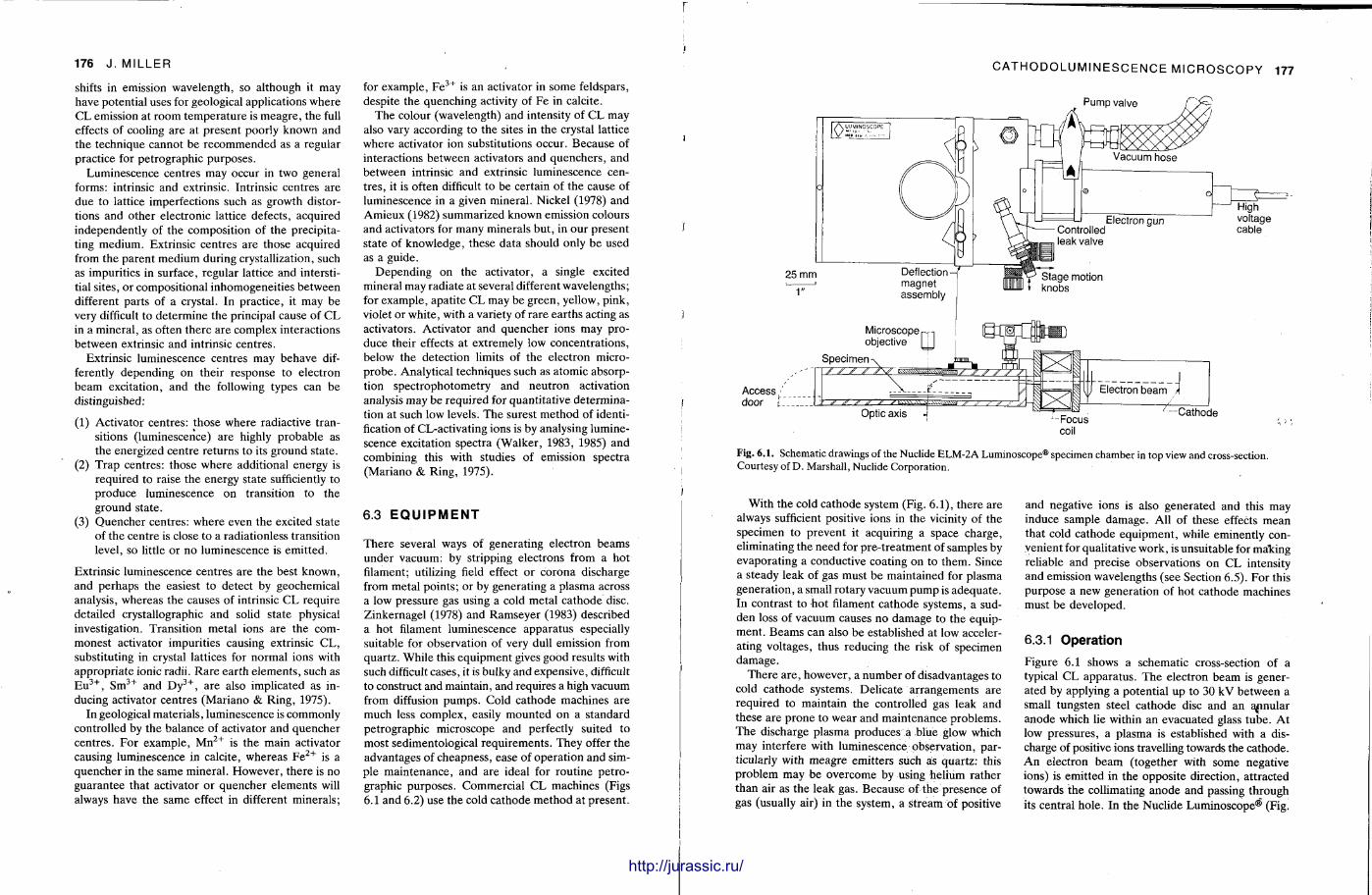
176 J . MILLER
shifts in emission wavelength, so although it may have potential uses for geological applications where C L emission at room tempera ture is meagre , the full effects of cooling are at present poorly known and the technique cannot be recommended as a regular practice for petrographic purposes.
Luminescence centres may occur in two general forms: intrinsic and extrinsic. Intrinsic centres are due to lattice imperfections such as growth distortions and other electronic lattice defects, acquired independently of the composition of the precipitating medium. Extrinsic centres are those acquired from the parent medium during crystallization, such as impurities in surface, regular lattice and interstitial sites, or compositional inhomogeneit ies between different parts of a crystal. In practice, it may be very difficult to determine the principal cause of C L in a mineral , as often there are complex interactions between extrinsic and intrinsic centres.
Extrinsic luminescence centres may behave differently depending on their response to electron beam excitation, and the following types can be distinguished:
(1) Activator centres: those where radiactive transitions (luminescence) are highly probable as the energized centre re turns to its ground state.
(2) T rap centres: those where additional energy is required to raise the energy state sufficiently to produce luminescence on transition to the ground state.
(3) Quencher centres: where even the excited state of the centre is close to a radiationless transition level, so little or no luminescence is emit ted.
Extrinsic luminescence centres are the best known, and perhaps the easiest to detect by geochemical analysis, whereas the causes of intrinsic C L require detailed crystallographic and solid state physical investigation. Transit ion metal ions are the commonest activator impurities causing extrinsic C L , substituting in crystal lattices for normal ions with appropria te ionic radii. R a r e ear th e lements , such as E u 3 + , S m 3 + and D y 3 + , are also implicated as inducing activator centres (Mariano & Ring, 1975).
In geological materials , luminescence is commonly controlled by the balance of activator and quencher centres . For example , M n 2 + is the main activator causing luminescence in calcite, whereas F e 2 + is a quencher in the same mineral . However , there is no guarantee that activator or quencher e lements will always have the same effect in different minerals;
for example , F e 3 + is an activator in some feldspars, despite the quenching activity of Fe in calcite.
The colour (wavelength) and intensity of CL may also vary according to the sites in the crystal lattice where activator ion substitutions occur. Because of interactions between activators and quenchers , and between intrinsic and extrinsic luminescence centres, it is often difficult to be certain of the cause of luminescence in a given mineral . Nickel (1978) and Amieux (1982) summarized known emission colours and activators for many minerals but , in our present state of knowledge, these data should only be used as a guide.
Depending on the activator, a single excited mineral may radiate at several different wavelengths; for example , apati te CL may be green, yellow, pink, violet or white , with a variety of rare ear ths acting as activators. Activator and quencher ions may produce their effects at extremely low concentrat ions, below the detection limits of the electron microprobe . Analytical techniques such as atomic absorption spectrophotometry and neut ron activation analysis may be required for quanti tat ive determination at such low levels. T h e surest method of identification of CL-activating ions is by analysing luminescence excitation spectra (Walker , 1983, 1985) and combining this with studies of emission spectra (Mariano & Ring, 1975).
6.3 E Q U I P M E N T
There several ways of generating electron beams under vacuum: by stripping electrons from a hot filament; utilizing field effect or corona discharge from metal points; or by generating a plasma across a low pressure gas using a cold metal ca thode disc. Zinkernagel (1978) and Ramseyer (1983) described a hot filament luminescence apparatus especially suitable for observation of very dull emission from quartz . While this equipment gives good results with such difficult cases, it is bulky and expensive, difficult to construct and maintain, and requires a high vacuum from diffusion pumps . Cold cathode machines are much less complex, easily mounted on a s tandard petrographic microscope and perfectly suited to most sedimentological requirements . They offer the advantages of cheapness , ease of operat ion and simple maintenance , and are ideal for rout ine pe t rographic purposes. Commercial CL machines (Figs 6.1 and 6.2) use the cold cathode method at present .
r
CATHODOLUMINESCENCE MICROSCOPY 177
Pump valve
25 mm
1"
High voltage cable
Deflection magnet assembly
Microscope p - , objective | i |
Specimen
Stage motion knobs
Optic axis -J - Focus coil
Cathode
Fig. 6 . 1 . Schematic drawings of the Nuclide ELM-2A Luminoscope® specimen chamber in top view and cross-section. Courtesy of D. Marshall, Nuclide Corporation.
With the cold cathode system (Fig. 6.1), there are always sufficient positive ions in the vicinity of the specimen t o prevent it acquiring a space charge, eliminating the need for pre- t rea tment of samples by evaporat ing a conductive coating on to them. Since a steady leak of gas must be maintained for plasma generat ion, a small ro tary vacuum p u m p is adequa te . In contrast to hot filament ca thode systems, a sudden loss of vacuum causes no damage to the equipment . Beams can also be established at low accelerating voltages, thus reducing the risk of specimen damage .
The re a re , however , a number of disadvantages to cold cathode systems. Delicate ar rangements are required to maintain the controlled gas leak and these are p rone to wear and maintenance problems. The discharge plasma produces a blue glow which may interfere with luminescence observation, particularly with meagre emitters such as quartz: this p rob lem may be overcome by using helium ra ther than air as the leak gas. Because of the presence of gas (usually air) in the system, a stream of positive
and negative ions is also generated and this may induce sample damage . All of these effects mean that cold cathode equipment , while eminently convenient for qualitative work, is unsuitable for malring reliable and precise observations on CL intensity and emission wavelengths (see Section 6.5). For this purpose a new generat ion of hot ca thode machines must be developed.
6.3.1 Operation
Figure 6.1 shows a schematic cross-section of a typical CL apparatus . T h e electron beam is generated by applying a potential up to 30 kV between a small tungsten steel ca thode disc and an annular anode which lie within an evacuated glass tube . A t low pressures, a plasma is established with a discharge of positive ions travelling towards the cathode. A n electron beam (together with some negative ions) is emitted in the opposite direction, at tracted towards t he collimating anode and passing through its central hole. In the Nuclide Luminoscope® (Fig.
http://jurassic.ru/
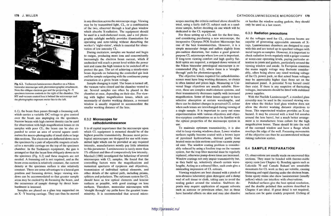
178 J . MILLER
Fig. 6 .2 . Technosyn luminescence chamber on a Nikon binocular microscope with photomicrographic attachment. Note the oblique electron gun and the projecting X—Y specimen traverse controls to the right of the chamber. The HT and vacuum control box is behind the microscope and the photographic exposure meter lies to the left.
6.1), the beam then passes through a focussing coil, which carries a variable D C voltage to give control over the beam size impinging on the specimen. Narrow beams with high current density can be used for observation with high magnification lenses or on samples with poor CL; the beam can be also expanded to cover an area of several square centimetres for macro-photography of small slabs or large thin sections. The electrons are deflected down on to the specimen by a pair of adjustable magnets attached to a movable carriage on the top of the specimen chamber . In the Technosyn equipment , the gun is arranged so that the beam fires obliquely down on to the specimen (Fig. 6.2) and these magnets are not needed . A focussing coil is not required, and as the beam cross-section is relatively constant , the current density at the specimen surface is also relatively constant . There are some advantages to a lateral gun position and focussing device; larger viewing windows can be accommodated so that greater sample areas may be excited by de-focussing the beam, and the occurrence of sample damage by direct bombardment is lessened.
Samples are placed on a glass tray suppor ted on an X—Y bearing carriage. They can thus be moved
in any direction across the microscope stage. Viewing may be by t ransmit ted light, C L , or a combinat ion of the two, observed through a lead glass window which absorbs X-radiat ion. The equipment should be used in a well-darkened room, and a red photographic safelight usefully provides illumination for operat ing and note-taking without disturbing the worker ' s 'night-vision', which is essential for observation of low intensity CL.
Dur ing excitation, samples are heated and begin to outgas, producing more ions and concomitantly increasingly the electron beam current , which if unchecked will reach a preset level within the power unit and cause the high tension to be switched off to protect the gun. The art of achieving a steady-state beam depends on balancing the controlled gas leak and the sample outgassing with the cont inuous p u m p evacuation at a given beam voltage.
Sample changing is rapid. The beam is turned off, the vacuum valve closed and the chamber vented to air. Several samples can often be placed in the chamber at once , depending on their size. For viewing with higher magnification lenses, which are necessarily of shorter working distance, a recessed window is usually required to accommodate the smaller working distance of the lens.
6.3.2 Microscopes for cathodoluminescence
It is of capital importance that the microscope upon which C L equipment is mounted should be of the highest possible transmissivity. Because most pe t rological microscopes are designed for use with transmitted light which can be provided at any required intensity, manufacturers mostly pay little at tention to this parameter . Luminescence is rarely more than 1% efficient and thus of comparatively low intensity. Marshall (1980) investigated the behaviour of several microscopes with C L samples. H e found that the controlling factors were the magnifications and numerical aper tures of eyepieces and objectives, transmission of individual optical e lements , and other details of the optical path , including prisms, splitters and polarizers. The opt imum system for CL should have as few optical elements and lens/air surfaces as possible, with good coatings on lens surfaces. Therefore , monocular microscopes with 'straight through ' ray paths have the greatest t ransmissivity. It is recommended that several micro-
CATHODOLUMINESCENCE MICROSCOPY 179
scopes meeting the criteria outlined above should be tr ied, using a fairly dull CL subject such as a sandstone sample, before deciding on one which will be dedicated to the CL equipment .
For those setting u p a C L unit for the first t ime, and considering purchasing a new microscope, the inexpensive Olympus P O S Student Microscope has one of the best transmissivities. However , it is a simple monocular design and suffers slightly from pin-cushion distortion, but makes a good general-purpose CL microscope where low cost is important . If long-term viewing comfort and high quality flat-field optics are required, a str ipped-down version of the Nikon binocular petrological microscope is recommended (Fig. 6.2), where there is a 'straight-through ' path for photomicrography.
T h e objective lenses required for cathodoluminescence must have long working distances, so choice is often limited and prices high. Measuring or Universal Stage objectives are usually suitable. However, these are complex multi-element systems, and their transmissivity decreases rapidly with increased magnification. Some of these lenses appear to have selective absorption at certain wavelengths, and there can be distinct changes in perceived CL colour when such lenses are interchanged during viewing of a single sample. It is important to carry out some experimentat ion with various objectives and objective-eyepiece combinations so as to be familiar with the optical propert ies of the microscope system in use.
To maintain opt imum transmissivity, it is also vital to keep viewing windows clean. Lower window surfaces rapidly become coated with a brown layer of pyrolized hydrocarbons, derived partly from heated resin on thin sections and from vacuum pump oil mist. The window coating problem is considerably reduced by using a foreline t rap on the vacuum system, but the t rap filter material must be regularly replaced, otherwise pump-down times are increased. Window coatings not only impair transmissivity but , as they build up , selectively absorb certain wavelengths. Acting as a coloured filter, such coats give a misleading impression of C L colours.
Viewing windows are best cleaned with a pinch of non-abrasive laboratory glass detergent and a damp wad of soft tissue or cloth, taking care to avoid the sealing gasket around the window. Stubborn deposits may require application Of organic solvents such as acetone or pet roleum ether , but as these have harmful effects on skin and may. also dissolve
or harden the window sealing gaskets, they should only be used as a last resort .
6.3.3 Radiation precautions
At the voltages used for CL, electron beams are capable of generating appreciable amounts of X-rays. Luminescence chambers are designed to cope with this and are tested up to specified voltages with metal targets as samples. However , it is important to check radiation levels regularly with a geiger counter at worst-case operat ing levels, paying particular attention to joints and gaskets, particularly around the viewing window and anode . In European countries the mains supply voltage may fluctuate considerably, often being above any ra ted working voltage of the CL power pack, so that actual beam voltages may be appreciably higher than those set on the instrument panel . A potential X-ray hazard could then exist. If there is any suspicion of fluctuating voltages, instruments should be fitted with stabilized power supplies.
With the Nuclide Luminoscope®, a standard glass coverslip may be used in the recessed viewing window when the thicker lead glass window does not allow the shorter working distance objectives t o focus. This unprotected window provides an X-ray hazard. It may be covered with a lead fo i lannulus around the lens barrel , but a much better arrangement is to manufacture brass collars for the high magnification lenses. These should fit into the well of the recessed window and have a flange which overlaps the edge of the well. Focussing movements of the objective can then be accommodated without risking radiation scatter.
6.4 S A M P L E P R E P A R A T I O N
CL observations are usually made on uncovered thin sections. They must be bonded with thermo-stable epoxy resin (see Chapter 4) . Bonding agents such as Lakeside 70 and Canada Balsam "are unsuitable mountants for CL work as they are volatile, causing blistering and rapid charring under the electron beam. Some epoxy resins also show luminescence (usually yellow) which can interfere with observations.
Polished surfaces give the best optical resolution, and the double polished thin sections described in Chapter 4 are ideal. If great detail is not required, surfaces can be quite crudely prepared . Etching of
http://jurassic.ru/
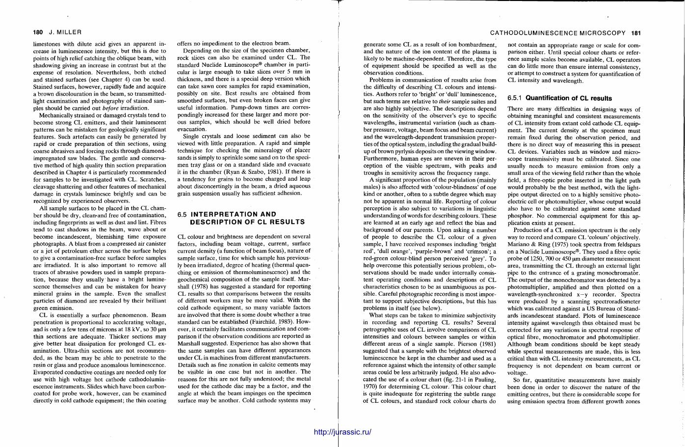
180 J . MILLER
l imestones with dilute acid gives an apparent increase in luminescence intensity, but this is due to points of high relief catching the oblique beam, with shadowing giving an increase in contrast but at the expense of resolution. Nevertheless, both etched and stained surfaces (see Chapter 4) can be used. Stained surfaces, however , rapidly fade and acquire a brown discolouration in the beam, so transmitted-light examination and photography of stained samples should be carried out before irradiation.
Mechanically strained or damaged crystals tend to become strong CL emit ters , and their luminescent pat terns can be mistaken for geologically significant features. Such artefacts can easily be generated by rapid or crude prepara t ion of thin sections, using coarse abrasives and forcing rocks through diamond-impregnated saw blades. The gentle and conservative method of high quality thin section preparat ion described in Chapte r 4 is particularly recommended for samples to be investigated with CL. Scratches, cleavage shattering and other features of mechanical damage in crystals luminesce brightly and can be recognized by experienced observers.
All sample surfaces to be placed in the C L chamber should be dry, clean-and free of contaminat ion, including fingerprints as well as dust and lint. Fibres tend to cast shadows in the beam, wave about or become incandescent, blemishing time exposure photographs . A blast from a compressed air canister or a jet of petroleum ether across the surface helps to give a contamination-free surface before samples are irradiated. It is also important to remove all t races of abrasive powders used in sample preparation, because they usually have a bright luminescence themselves and can be mistaken for heavy mineral grains in the sample. Even the smallest particles of d iamond are revealed by their brilliant green emission.
CL is essentially a surface phenomenon . Beam penetra t ion is proport ional to accelerating voltage, and is only a few tens of microns at 18 kV, so 30 um thin sections are adequate . Thicker sections may give bet ter heat dissipation for prolonged CL examinat ion. Ultra-thin sections are not recommended, as the beam may be able to penet ra te to the resin or glass and produce anomalous luminescence. Evapora ted conductive coatings are needed only for use with high voltage hot cathode cathodoluminescence instruments . Slides which have been carbon-coated for probe work, however , can be examined directly in cold cathode equipment ; the thin coating
offers no impediment to the electron beam. Depending on the size of the specimen chamber ,
rock slices can also be examined under CL. The standard Nuclide Luminoscope® chamber in particular is large enough to take slices over 5 mm in thickness, and there is a special deep version which can take sawn core samples for rapid examinat ion, possibly on site. Best results are obtained from smoothed surfaces, but even broken faces can give useful information. Pump-down times a re correspondingly increased for these larger and more porous samples, which should be well dried before evacuation.
Single crystals and loose sediment can also be viewed with little prepara t ion . A rapid and simple technique for checking the mineralogy of placer sands is simply to sprinkle some sand on to the specimen tray glass or on a standard slide and evacuate it in the chamber (Ryan & Szabo, 1981). If there is a tendency for grains to become charged and leap about disconcertingly in the beam, a dried aqueous grain suspension usually has sufficient adhesion.
6.5 I N T E R P R E T A T I O N A N D D E S C R I P T I O N O F C L R E S U L T S
CL colour and brightness are dependent on several factors, including beam voltage, current , surface current density (a function of beam focus), na ture of sample surface, t ime for which sample has previously been irradiated, degree of heating ( thermal quenching or emission of thermoluminescence) and the geochemical composition of the sample itself. Marshall (1978) has suggested a s tandard for report ing CL results so that comparisons between the results of different workers may be more valid. With the cold cathode equipment , so many variable factors are involved that there is some doubt whether a t rue s tandard can be established (Fairchild, 1983). However, it certainly facilitates communicat ion and comparison if the observation conditions are repor ted as Marshall suggested. Experience has also shown that the same samples can have different appearances under C L in machines from different manufacturers . Details such as fine zonation in calcite cements may be visible in one case but not in another . The reasons for this are not fully unders tood; the metal used for the cathode disc may be a factor, and the angle at which the beam impinges on the specimen surface may be another . Cold cathode systems may
CATHODOLUMINESCENCE MICROSCOPY 181
generate some C L as a result of ion bombardmen t , and the na ture of the ion content of the plasma is likely to be machine-dependent . Therefore , the type of equipment should be specified as well as the observation conditions.
Problems in communicat ion of results arise from the difficulty of describing CL colours and intensities. Authors refer to 'bright ' or 'dull ' luminescence, but such terms are relative to their sample suites and are also highly subjective. The descriptions depend on the sensitivity of the observer 's eye to specific wavelengths, instrumental variation (such as chamber pressure , voltage, beam focus and beam current) and the wavelength-dependent transmission properties of the optical system, including the gradual buildup of brown pyrlysis deposits on the viewing window. Fur the rmore , human eyes are uneven in their perception of the visible spectrum, with peaks and troughs in sensitivity across the frequency range.
A significant propor t ion of the populat ion (mainly males) is also affected with 'colour-blindness' of one kind or another , often to a subtle degree which may not be apparent in normal life. Repor t ing of colour percept ion is also subject to variations in linguistic unders tanding of words for describing colours. These are learned at an early age and reflect the bias and background of our parents . U p o n asking a number of people to describe the C L colour of a given sample, I have received responses including 'bright red ' , 'dull o range ' , 'purple-brown' and 'cr imson' ; a red-green colour-blind person perceived 'grey' . To help overcome this potentially serious problem, observations should be m a d e under internally consistent operat ing conditions and descriptions of CL characteristics chosen to be as unambiguous as possible. Careful photographic recording is most important to support subjective descriptions, but this has problems in itself (see below).
Wha t steps can be taken to minimize subjectivity in recording and report ing C L results? Several petrographic uses of C L involve comparisons of C L intensities and colours between samples or within different areas of a single sample. Pierson (1981) suggested that a sample with the brightest observed luminescence be kept in the chamber and used as a reference against which the intensity of o ther sample areas could be less arbitrarily judged. H e also advocated the use of a colour chart (fig, 21-1 in Pauling, 1970) for determining CL colour. This colour chart is quite inadequate for registering the subtle range of CL colours, and s tandard rock colour charts do
not contain an appropr ia te range or scale for comparison either. Until special colour charts or reference sample scales become available, C L operators can do little more than ensure internal consistency, or a t tempt to construct a system for quantification of C L intensity and wavelength.
6.5.1 Quantif ication of CL results
There are many difficulties in designing ways of obtaining meaningful and consistent measurements of CL intensity from extant cold cathode CL equipment . The current density at the specimen must remain fixed during the observation period, and there is no direct way of measuring this in present CL devices. Variables such as window and microscope transmissivity must be calibrated. Since one usually needs to measure emission from only a small area of the viewing field ra ther than the whole field, a fibre-optic p robe inserted in the light path would probably be the best me thod , with the light-pipe ou tpu t directed on to a highly sensitive pho toelectric cell or photomult ipl ier , whose output would also have to be calibrated against some standard phosphor . N o commercial equipment for this application exists at present .
Production of a C L emission spectrum is the only way to record and compare CL 'colours ' objectively. Mar iano & Ring (1975) took spectra from feldspars on a Nuclide Luminoscope®. They used a fibre optic probe of 1250, 700 or 450 um diameter measurement area , transmitting the C L through an external light pipe t o the ent rance of a grating monochromator . The output of the monochromator was detected by a photomult ipl ier , amplified and then plot ted on a wavelength-synchronized x—y recorder . Spectra were produced by a scanning spectroradiometer which was calibrated against a U S Bureau of Standards incandescent s tandard. Plots of luminescence intensity against wavelength thus obtained must be corrected for any variations in spectral response of optical fibre, monochromator and photomultiplier. Al though beam conditions should be kept steady while spectral measurements are m a d e , this is less critical than with C L intensity measurements , as CL frequency is not dependent on beam current or voltage.
So far, quanti tat ive measurements have mainly been done in order to discover the nature of the emitting centres, but there is considerable scope for using emission spectra from different growth zones
mmmm http://jurassic.ru/
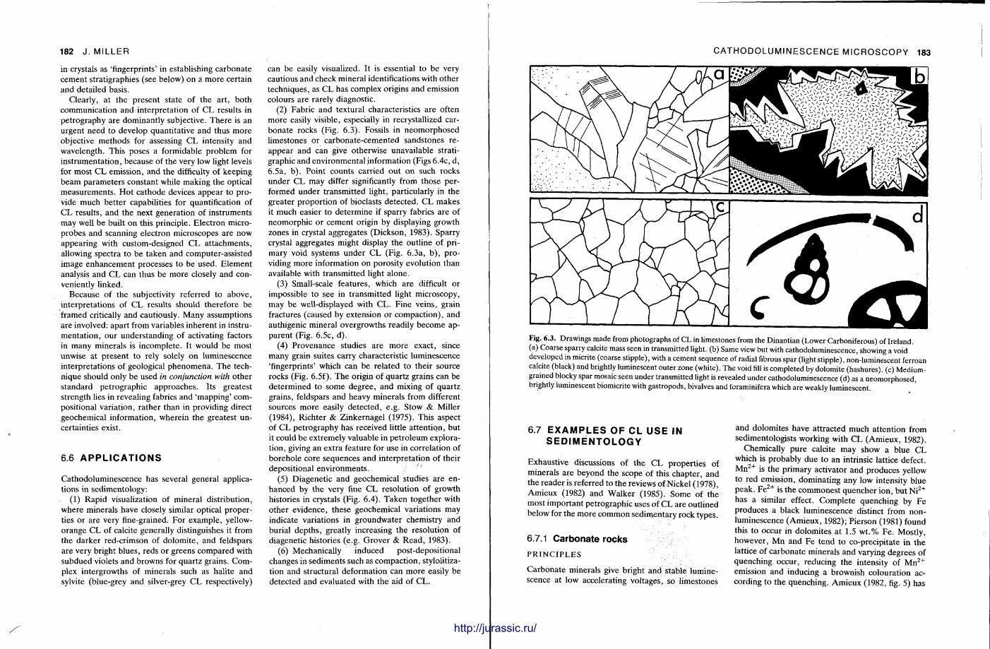
182 J . MILLER
in crystals as 'fingerprints' in establishing carbonate cement stratigraphies (see below) on a more certain and detailed basis.
Clearly, at the present state of the art , both communication and interpretat ion of C L results in petrography are dominantly subjective. The re is an urgent need to develop quanti tat ive and thus more objective methods for assessing CL intensity and wavelength. This poses a formidable problem for instrumentat ion, because of the very low light levels for most C L emission, and the difficulty of keeping beam parameters constant while making the optical measurements . Ho t ca thode devices appear to provide much bet ter capabilities for quantification of CL results, and the next generat ion of instruments may well be built on this principle. Electron micro-probes and scanning electron microscopes are now appearing with custom-designed C L at tachments , allowing spectra to be taken and computer-assisted image enhancement processes to be used. E lement analysis and CL can thus be more closely and conveniently linked.
Because of the subjectivity referred to above, interpretat ions of C L results should therefore be framed critically and cautiously. Many assumptions are involved: apart from variables inherent in instrumentat ion, our unders tanding of activating factors in many minerals is incomplete . It would be most unwise at present to rely solely on luminescence interpretat ions of geological phenomena . The technique should only be used in conjunction with other standard petrographic approaches . Its greatest strength lies in revealing fabrics and 'mapping ' compositional variation, ra ther than in providing direct geochemical information, wherein the greatest uncertainties exist.
6.6 A P P L I C A T I O N S
Cathodoluminescence has several general applications in sedimentology:
(1) Rapid visualization of mineral distribution, where minerals have closely similar optical properties or are very fine-grained. For example , yellow-orange CL of calcite generally distinguishes it from the darker red-crimson of dolomite , and feldspars are very bright blues, reds or greens compared with subdued violets and browns for quar tz grains. Complex intergrowths of minerals such as halite and sylvite (blue-grey and silver-grey CL respectively)
can be easily visualized. It is essential to be very cautious and check mineral identifications with other techniques, as C L has complex origins and emission colours are rarely diagnostic.
(2) Fabric and textural characteristics are often more easily visible, especially in recrystallized carbonate rocks (Fig. 6.3). Fossils in neomorphosed limestones or carbonate-cemented sandstones reappear and can give otherwise unavailable stratigraphic and environmental information (Figs 6.4c, d, 6.5a, b ) . Point counts carried ou t on such rocks under CL may differ significantly from those performed under transmitted light, particularly in the greater proport ion of bioclasts detected. C L makes it much easier to determine if sparry fabrics are of neomorphic or cement origin by displaying growth zones in crystal aggregates (Dickson, 1983). Sparry crystal aggregates might display the outline of primary void systems under CL (Fig. 6.3a, b ) , p roviding more information on porosity evolution than available with t ransmit ted light a lone.
(3) Small-scale features, which are difficult or impossible to see in transmitted light microscopy, may be well-displayed with CL . Fine veins, grain fractures (caused by extension or compact ion) , and authigenic mineral overgrowths readily become apparent (Fig. 6.5c, d) .
(4) Provenance studies are more exact, since many grain suites carry characteristic luminescence 'fingerprints' which can be related to their source rocks (Fig: 6.5f). The origin of quartz grains can be determined to some degree, and mixing of quartz grains, feldspars and heavy minerals from different sources more easily detected, e.g. Stow & Miller (1984), Richter & Zinkernagel (1975). This aspect of CL petrography has received little a t tent ion, but it could be extremely valuable in pe t ro leum explorat ion, giving an extra feature for use in correlation of borehole core sequences and interpretat ion of their depositional environments .
(5) Diagenet ic and geochemical studies are enhanced by the very fine C L resolution of growth histories in crystals (Fig. 6.4). Taken together with other evidence, these geochemical variations may indicate variations in groundwater chemistry and burial depths , greatly increasing the resolution of diagenetic histories (e.g. Grover & R e a d , 1983).
(6) Mechanically induced post-deposit ional changes in sediments such as compact ion, stylolitiza-tion and structural deformation can more easily be detected and evaluated with the aid of CL.
ill
CATHODOLUMINESCENCE MICROSCOPY 183
Fig. 6.3. Drawings made from photographs of CL in limestones from the Dinantian (Lower Carboniferous) of Ireland. (a) Coarse sparry calcite mass seen in transmitted light, (b) Same view but with cathodoluminescence, showing a void developed in micrite (coarse stipple), with a cement sequence of radial fibrous spar (light stipple), non-luminescent ferroan calcite (black) and brightly luminescent outer zone (white). The void fill is completed by dolomite (hashures). (c) Medium-grained blocky spar mosaic seen under transmitted light is revealed under cathodoluminescence (d) as a neomorphosed, brightly luminescent biomicrite with gastropods, bivalves and foraminifera which are weakly luminescent.
6.7 E X A M P L E S OF C L USE IN S E D I M E N T O L O G Y
Exhaustive discussions of the C L propert ies of minerals are beyond the scope of this chapter , and the reader is referred to t he reviews of Nickel (1978), Amieux (1982) and Walker (1985). Some of the most important petrographic uses of C L are outl ined below for the more common sedimentary rock types.
6.7.1 Carbonate rocks
P R I N C I P L E S
Carbona te minerals give bright and stable luminescence at low accelerating voltages, so limestones
and dolomites have at tracted much at tent ion from sedimentologists working with C L (Amieux, 1982).
Chemically pure calcite may show a blue CL which is probably due to an intrinsic lattice defect. M n 2 + is the pr imary activator and produces yellow to red emission, dominat ing any low intensity blue peak. F e 2 + is the commonest quencher ion, but N i 2 +
has a similar effect. Comple te quenching by Fe produces a black luminescence distinct from non-luminescence (Amieux, 1982); Pierson (1981) found this to occur in dolomites at 1.5 wt .% Fe . Mostly, however , M n and Fe t end to co-precipitate in the lattice of carbonate minerals and varying degrees of quenching, occur, reducing the intensity of M n 2 +
emission and inducing a brownish colouration according to the quenching. Amieux (1982, fig. 5) has
http://jurassic.ru/
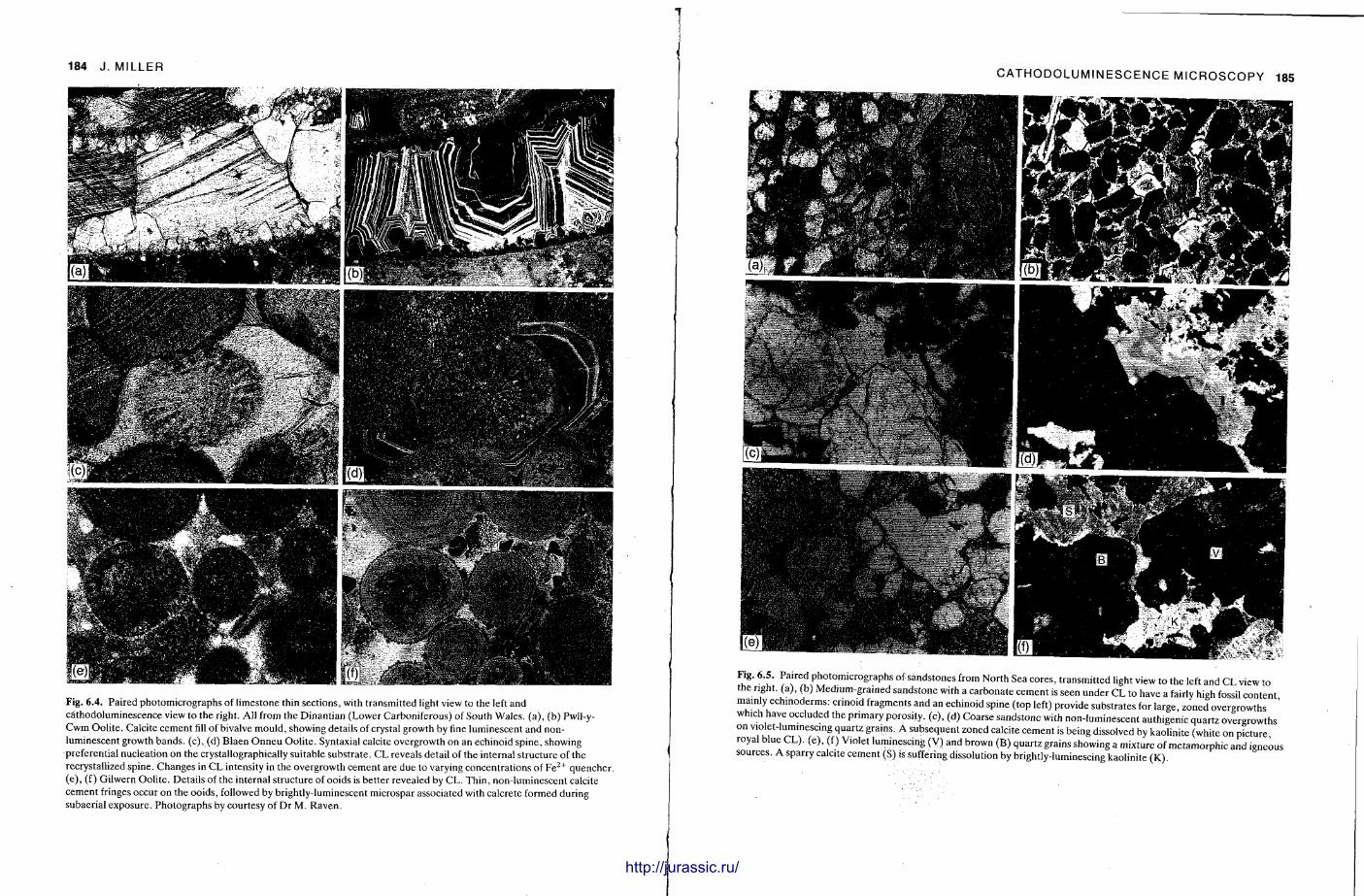
184 J . MILLER
Fig. 6.4. Paired photomicrographs of limestone thin sections, with transmitted light view to the left and cathodoluminescence view to the right. All from the Dinantian (Lower Carboniferous) of South Wales, (a), (b) Pwll-y-Cwm Oolite. Calcite cement fill of bivalve mould, showing details of crystal growth by fine luminescent and non-luminescent growth bands, (c), (d) Blaen Onneu Oolite. Syntaxial calcite overgrowth on an echinoid spine, showing preferential nucleation on the crystallographically suitable substrate. CL reveals detail of the internal structure of the recrystallized spine. Changes in CL intensity in the overgrowth cement are due to varying concentrations of F e 2 + quencher, (e), (f) Gilwern Oolite. Details of the internal structure of ooids is better revealed by CL. Thin, non-luminescent calcite cement fringes occur on the ooids, followed by brightly-luminescent microspar associated with calcrete formed during subaerial exposure. Photographs by courtesy of Dr M. Raven.
CATHODOLUMINESCENCE MICROSCOPY 185
Fig. 6.5. Paired photomicrographs of sandstones from North Sea cores, transmitted light view to the left and CL view to the right, (a), (b) Medium-grained sandstone with a carbonate cement is seen under CL to have a fairly high fossil content, mainly echinoderms: crinoid fragments and an echinoid spine (top left) provide substrates for large, zoned overgrowths which have occluded the primary porosity, (c), (d) Coarse sandstone with non-luminescent authigenic quartz overgrowths on violet-luminescing quartz grains. A subsequent zoned calcite cement is being dissolved by kaolinite (white on picture, royal blue CL). (e), (f) Violet luminescing (V) and brown (B) quartz grains showing a mixture of metamorphic and igneous sources. A sparry calcite cement (S) is suffering dissolution by brightly-luminescing kaolinite (K).
http://jurassic.ru/
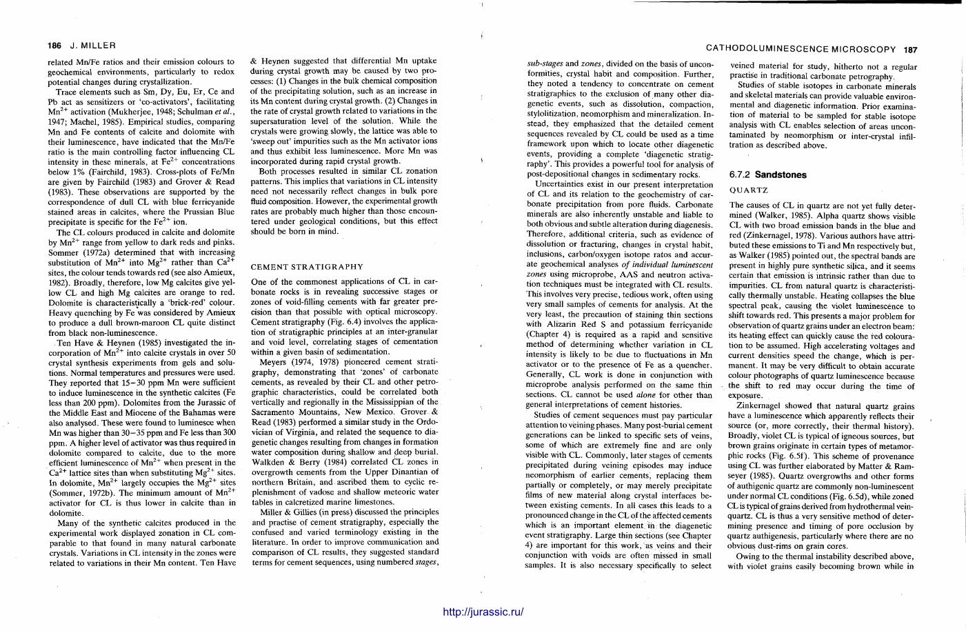
186 J . MILLER
& Heynen suggested that differential Mn up take dur ing crystal growth may be caused by two processes: (1) Changes in the bulk chemical composition of the precipitating solution, such as an increase in its M n content during crystal growth. (2) Changes in the rate of crystal growth related to variations in the supersaturat ion level of the solution. While the crystals were growing slowly, the lattice was able to 'sweep out ' impurities such as the Mn activator ions and thus exhibit less luminescence. More Mn was incorporated during rapid crystal growth.
Both processes resulted in similar C L zonat ion pat terns . This implies that variations in C L intensity need not necessarily reflect changes in bulk pore fluid composition. However, the experimental growth rates are probably much higher than those encountered under geological condit ions, but this effect should be born in mind.
C E M E N T S T R A T I G R A P H Y
O n e of the commonest applications of C L in carbonate rocks is in revealing successive stages o r zones of void-filling cements with far greater precision than that possible with optical microscopy. Cement stratigraphy (Fig. 6.4) involves the application of stratigraphic principles at an inter-granular and void level, correlating stages of cementat ion within a given basin of sedimentat ion.
Meyers (1974, 1978) pioneered cement stratigraphy, demonstrat ing that 'zones ' of carbonate cements , as revealed by their CL and other pe t rographic characteristics, could be correlated both vertically and regionally in the Mississippian of the Sacramento Mounta ins , New Mexico. Grover & R e a d (1983) performed a similar study in the Ordo-vician of Virginia, and related the sequence to diagenetic changes resulting from changes in formation water composit ion during shallow and d e e p burial . Walkden & Berry (1984) correlated C L zones in overgrowth cements from the U p p e r Dinant ian of nor thern Britain, and ascribed them to cyclic replenishment of vadose and shallow meteoric water tables in calcretized mar ine limestones.
Miller & Gillies (in press) discussed the principles and practise of cement stratigraphy, especially the confused and varied terminology existing in the l i terature. In order to improve communicat ion and comparison of C L results, they suggested s tandard terms for cement sequences, using numbered stages,
I
CATHODOLUMINESCENCE MICROSCOPY 187
sub-stages and zones, divided on the basis of unconformities, crystal habit and composition. Fur ther , they noted a tendency to concentrate on cement stratigraphies to the exclusion of many other diagenetic events, such as dissolution, compact ion, stylolitization, neomorphism and mineralization. Instead, they emphasized that the detailed cement sequences revealed by CL could be used as a t ime framework upon which to locate other diagenetic events, providing a complete 'diagenetic stratigraphy ' . This provides a powerful tool for analysis of post-depositional changes in sedimentary rocks.
Uncertaint ies exist in our present interpretat ion of CL and its relation to the geochemistry of carbonate precipitation from pore fluids. Carbonate minerals are also inherently unstable and liable to both obvious and subtle alteration during diagenesis. Therefore , additional criteria, such as evidence of dissolution or fracturing, changes in crystal habit , inclusions, carbon/oxygen isotope ratos and accurate geochemical analyses of individual luminescent zones using microprobe, A A S and neutron activation techniques must be integrated with CL results. This involves very precise, tedious work, often using very small samples of cements for analysis. At the very least, the precaution of staining thin sections with Alizarin Red S and potassium ferricyanide (Chapter 4) is required as a rapid and sensitive method of determining whether variation in CL intensity is likely to be due to fluctuations in Mn activator or to the presence of Fe as a quencher . General ly , C L work is done in conjunction with microprobe analysis performed on the same thin sections. CL cannot be used alone for other than general interpretat ions of cement histories.
Studies of cement sequences must pay particular at tention to veining phases . Many post-burial cement generat ions can be linked to specific sets of veins, some of which are extremely fine and are only visible with CL. Commonly , later stages of cements precipitated during veining episodes may induce neomorphism of earlier cements , replacing them partially or completely, or may merely precipitate films of new material along crystal interfaces between existing cements . In all cases this leads to a pronounced change in the C L o f the affected cements which is an important e lement in the diagenetic event stratigraphy. Large thin sections (see Chapter 4) are important for this work, as veins and their conjunction with voids are often missed in small samples. It is also necessary specifically to select
veined material for study, hi therto not a regular practise in traditional carbonate petrography.
Studies of stable isotopes in carbonate minerals and skeletal materials can provide valuable environmental and diagenetic information. Prior examination of material to be sampled for stable isotope analysis with C L enables selection of areas uncon-taminated by neomorphism or inter-crystal infilt rat ion as described above.
6.7.2 Sandstones
Q U A R T Z
The causes of CL in quartz are not yet fully determined (Walker , 1985). Alpha quartz shows visible C L with two broad emission bands in t he blue and red (Zinkernagel , 1978). Various authors have attributed these emissions to Ti and M n respectively but , as Walker (1985) pointed out , the spectral bands are present in highly pure synthetic silica, and it seems certain that emission is intrinsic rather than due to impurit ies. C L from natural quar tz is characteristically thermally unstable. Heat ing collapses the blue spectral peak , causing the violet luminescence to shift towards red. This presents a major problem for observation of quartz grains under an electron beam: its heat ing effect can quickly cause the fed colouration to be assumed. High accelerating voltages and current densities speed the change, which is permanent . It may be very difficult to obtain accurate colour photographs of quar tz luminescence because the shift to red may occur during the time of exposure.
Zinkernagel showed that natural quar tz grains have a luminescence which apparently reflects their source (or, more correctly, their thermal history). Broadly, violet C L is typical of igneous sources, but brown grains originate in certain types of metamorphic rocks (Fig. 6.5f). This scheme of provenance using CL was further e laborated by Mat te r & Ram-seyer (1985). Quar tz overgrowths and other forms of authigenic quartz are commonly non-luminescent under normal CL conditions (Fig. 6.5d), while zoned CL is typical of grains derived from hydrothermal vein-quartz . CL is thus a very sensitive method of determining presence and timing of pore occlusion by quartz authigenesis, particularly where there are no obvious dust-rims on grain cores.
Owing to the thermal instability described above, with violet grains easily becoming brown while in
related Mn/Fe ratios and their emission colours to geochemical environments , particularly to redox potential changes during crystallization.
Trace elements such as Sm, Dy, E u , E r , Ce and Pb act as sensitizers or 'co-activators ' , facilitating M n 2 + activation (Mukher jee , 1948; Schulman etal., 1947; Machel , 1985). Empirical studies, comparing Mn and Fe contents of calcite and dolomite with their luminescence, have indicated that the Mn/Fe ratio is the main controlling factor influencing CL intensity in these minerals , at F e 2 + concentrat ions below 1% (Fairchild, 1983). Cross-plots of Fe /Mn are given by Fairchild (1983) and Grover & Read (1983). These observations are supported by the correspondence of dull CL with blue ferricyanide stained areas in calcites, where the Prussian Blue precipitate is specific for the F e 2 + ion.
T h e CL colours produced in calcite and dolomite by M n 2 + range from yellow to dark reds and pinks. Sommer (1972a) determined that with increasing substitution of M n 2 + into M g 2 + ra ther than C a 2 +
sites, the colour tends towards red (see also Amieux, 1982). Broadly, therefore, low Mg calcites give yellow CL and high Mg calcites are orange to red. Dolomite is characteristically a 'brick-red' colour. Heavy quenching by Fe was considered by Amieux to produce a dull brown-maroon CL quite distinct from black non-luminescence.
Ten Have & Heynen (1985) investigated the incorporat ion of M n 2 + into calcite crystals in over 50 crystal synthesis experiments from gels and solutions. Normal temperatures and pressures were used. They repor ted that 1 5 - 3 0 ppm Mn were sufficient to induce luminescence in the synthetic calcites (Fe less than 200 ppm) . Dolomites from the Jurassic of the Middle East and Miocene of the Bahamas were also analysed. These were found to luminesce when Mn was higher than 3 0 - 3 5 ppm and Fe less than 300 ppm. A higher level of activator was thus required in dolomite compared to calcite, due to the more efficient luminescence of M n 2 + when present in the C a 2 + lattice sites than when substituting M g 2 + sites. In dolomite , M n 2 + largely occupies the M g 2 + sites (Sommer, 1972b). T h e minimum amount of M n 2 +
activator for CL is thus lower in calcite than in dolomite .
Many of the synthetic calcites produced in the experimental work displayed zonation in CL comparable to that found in many natural carbonate crystals. Variations in C L intensity in the zones were related to variations in their Mn content . Ten Have
http://jurassic.ru/
188 J . MILLER
the electron beam, much care and some skill is needed to distinguish quar tz C L colours successfully. Given this, CL affords a rapid means of detecting different quartz grain populat ions in sandstones and in ascertaining their provenance. The different shades of violet and brown in a grain populat ion probably represent various grain sources, since there is no evidence that crystal orientation exerts significant control over CL wavelength and intensity in quartz . Of course, it is wise to check the other propert ies of the grains, such as inclusions and type of extinction, to gain confirmation of C L determinations.
Sippel (1968) and Sibley & Blatt (1976) have applied C L in investigations of silica authigenesis in sandstones. Burley, Kantorowicz & Waugh (1985) suggested how CL may profitably be combined with other techniques in elucidating diagenesis of clastic rocks.
F E L D S P A R S
The causes of C L in this mineral group are relatively well-known from investigations on lunar rocks (Geake et al., 1977) and-carbonati tes (Mar iano , I to & Ring, 1973). Feldspars have low CL thresholds and are thus obvious even at low accelerating voltages. Typical CL colours are brilliant blue (possibly T i 2 + activation), red to infra-red ( F e 3 + substitution for A l 3 + ) and green ( M n 2 + substitution probably for C a 2 + ) . Feldspar C L is polarized and some intensity variation is seen upon rotat ion of a polaroid sheet interposed between the viewing window and the microscope eyepiece. This property often helps to distinguish feldspars from other minerals of similar CL colour. In general , authigenic feldspars are non-luminescent or very dully luminescent (Kastner , 1971), serving to differentiate detrital cores from their overgrowths.
In terms of provenance , there is no evidence to suggest that feldspar C L is related to specific igneous or metamorphic origins. However , the presence of feldspar 'suites ' containing consistent proport ions of the rarer red and/or green emitter grains amongst the common blue emitters can be used to trace particular sources of clastic feldspar supply (e.g. Stow & Miller, 1984).
Because even the smallest feldspar grains luminesce brightly, a far more accurate est imate of the percentage of feldspar in a clastic sediment is
obtained by point-counting under CL . This is particularly t rue for fine sandstones and siltstones. Even grains which are badly weathered or altered still register the typical emission.
H E A V Y M I N E R A L S
Many accessory minerals of clastic rocks contain at least traces of rare ear th or transition metal impurities and are therefore liable to luminesce. Nickel (1978) listed the known CL characteristics of such minerals. Apat i tes give particularly bright C L , with europium a common activator (Mariano & Ring, 1975). Apat i te emissions range from bluish-violet, lilac, pink and orange to yellow. Portnov & Gorobe t s (1969) have proposed that certain of these colours are related to particular igneous or metamorphic origins. If this can be confirmed, it would be an invaluable adjunct to provenance studies. Again , the small size of many heavy mineral grains means that they are often overlooked and easily underestimated in t ransmit ted light petrography of clastic rocks. Invariably, use of CL produces an often surprising re-evaluation of the importance of accessory grains.
C E M E N T S A N D D I A G E N E S I S
Carbonate cements are commonly involved in occlusion of sandstone porosity (Fig. 6.5b, f ) . Their mineralogy and sequence of development are more accurately followed by using C L than by t ransmit ted light alone (see above) . O the r diagenetic features such as corrosion of quar tz grains by carbonate , relative timing of quar tz overgrowth formation and cementat ion and the onset of dolomitization can also be rapidly documented with CL. Authigenic kaolinite or dickite commonly form late stage cements in sandstones (Fig. 6.5f, Burley et al., 1985, fig. 7f ) , and they usually have a brilliant royal blue C L , whose origin is unknown. T h e extent and timing of these cements and their relationship to compaction and tectonic events , such as extension veining, is much more easily appreciated under C L than with transmitted light microscopy.
A good example of the combined use of C L , S E M and transmit ted light petrography in document ing the provenance and diagenetic history of a Jurassic reservoir sandstone is given by Olaussen et al. (1984).
6.8 P H O T O G R A P H I C R E C O R D I N G OF C L
Prior to the realization that high transmissivity microscopes were mandatory for successful CL work, photography of C L was extremely difficult and the results highly variable. Minerals giving very low intensity emission, such as quartz grains, required many minutes or even hours of exposure with fast films. General ly, these films were working at luminance ranges beyond their zones of reciprocity failure, resulting in poor resolution, low contrast and indifferent colour rendit ion. Good microscope transmissivity, aided by straight-through light paths between objective and film, means that slower (and thus finer-grained) films can now be used, working well within their opt imum exposure ranges.
Most petrological microscopes can be fitted with photomicrography accessories which allow automatic exposure determinat ion (Fig. 6.3). The large viewing window of the Nuclide Luminoscope® also allows the use of a 55 m m / 7 3 . 5 macro lens directly mounted on a camera body to take pictures of whole thin sections or slabs under CL . Such pictures are invaluable for mapping CL zones in carbonate cements whch are to be sampled for A A S and stable isotope analysis by drilling or scraping from individual cement stages. They also show up fabrics and small-scale sedimentary structures in sandstones and siltstones.
Recent advances in film technology have increased the range of films suitable for C L recording. For rout ine work, particularly with l imestones, where the colour range is restricted and can be adequately represented in grey tones , black and white films are satisfactory. Invariably, good quality prints will show up more detail than was apparent to the observer viewing the C L , because of fatigue and insensitivity of the eye at low light levels. Suitable films are medium-speed types ( ISO 125—400) which possess fine grain, good contrast range and some exposure lat i tude, such as Ilford FP4 or X P 1 . Normally, paired exposures are made , one showing the transmitted light view and one the C L view. CL negatives often have a somewhat restricted contrast range, and these 'flat' negatives may be enhanced by printing on harder paper than the transmitted light frames.
Sandstones are difficult subjects; quartz CL is very subdued but feldspars are very bright, often with a high U V component . It is almost impossible
HODOLUMINESCENCE MICROSCOPY 189
to get brilliant and dark grains properly exposed on the same frame. Correct exposure for dull quar tz usually results in serious over-exposure of feldspars, with development of halation areas around the grains, while correct exposure of feldspars produces marked under-exposure of quar tz grains. A series of half-stop under- and over-exposure gradations will usually produce one frame which is satisfactory for each. Correct ion can also be done by changing the film speed between exposures on an automatic centre-weighted averaging meter — setting a slower film speed will trick the meter into underexposing a bright grain. A light meter with a movable spot, as in the Nikon system (Fig. 6.3) can provide direct exposure readings for particular grains.
It is also important , with porous rocks, to remove carefully all t races of the diamond polishing abrasives from the slide: industrial d iamond grains have a brilliant green CL which produces halation spots, giving the impression of a larger grain, which is apt to be mistaken for an apati te or other heavy mineral grain.
Colour pictures are somewhat more problematic , in that the precise colours of C L are very difficult to reproduce exactly. Daylight films give the best colour balance, with a blue compensat ing filter for the transmitted light ( tungsten lamp) frames. The choice lies between print films with a narrower contrast range and variable colour balance depending on printing filtration, and reversal films with a higher contrast and resolution range bu t where subsequent correction is not possible. Agfa, Kodak and Fuji produce ranges of colour slide and print films ranging from I S O 25 to 1000, with an H R suffix indicating the films' high resolution capability by virtue of the very thin emulsions used in the colour separation layers. T h e slower t he speed, t he finer the grain and the greater the resolving power of these films. ISO 1000 films may be needed to collect CL images of thermally unstable quar tz grains which rapidly redden under excitation. Each worker is advised to exper iment with a range of films, both colour and monochrome , and then to become thoroughly familiar with those which are best suited.
C L depends so often on rendition of a range of colours, some soft and subtle, some brilliant, that op t imum report ing of CL studies in publications may demand expensive colour plates. While monochrome C L images are adequa te for l imestones, as noted above, sandstone CL recorded in mono-
http://jurassic.ru/
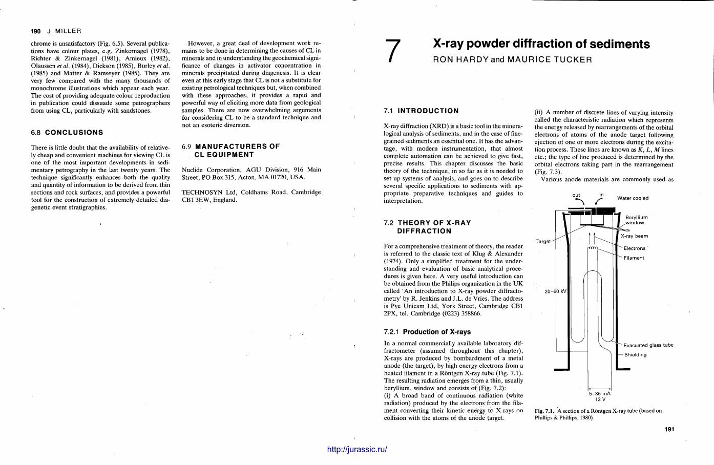
190 J . MILLER
chrome is unsatisfactory (Fig. 6.5). Several publications have colour plates, e.g. Zinkernagel (1978), Richter & Zinkernagel (1981), Amieux (1982), Olaussen et al. (1984), Dickson (1985), Burley et al. (1985) and Mat ter & Ramseyer (1985). They are very few compared with the many thousands of monochrome illustrations which appear each year. The cost of providing adequa te colour reproduct ion in publication could dissuade some pet rographers from using C L , particularly with sandstones.
6.8 C O N C L U S I O N S
There is little doubt that the availability of relatively cheap and convenient machines for viewing C L is one bf the most impor tant developments in sedimentary petrography in the last twenty years. The technique significantly enhances both the quality and quantity of information to be derived from thin sections and rock surfaces, and provides a powerful tool for the construction of extremely detailed diagenetic event stratigraphies.
However , a great deal of development work remains to be done in determining the causes of C L in minerals and in unders tanding the geochemical significance of changes in activator concentrat ion in minerals precipitated during diagenesis. It is clear even at this early stage that CL is not a substitute for existing petrological techniques but , when combined with these approaches , it provides a rapid and powerful way of eliciting more data from geological samples. There are now overwhelming arguments for considering C L to be a s tandard technique and not an esoteric diversion.
6 .9 M A N U F A C T U R E R S OF C L E Q U I P M E N T
Nuclide Corpora t ion , A G U Division, 916 Main Street , P O Box 315, Acton , M A 01720, U S A .
T E C H N O S Y N Ltd , Coldhams Ro ad , Cambridge CB1 3 E W , England.
7 X-ray powder diffraction of sediments RON HARDYand MAURICE TUCKER
7.1 I N T R O D U C T I O N
X-ray diffraction ( X R D ) is a basic tool in the mineralogical analysis of sediments , and in the case of finegrained sediments an essential one . It has the advantage, with modern ins t rumentat ion, that almost complete automat ion can be achieved to give fast, precise results. This chapter discusses the basic theory of the technique, in so far as it is needed to set up systems of analysis, and goes on to describe several specific applications to sediments with appropr ia te preparat ive techniques and guides to interpretat ion.
7.2 T H E O R Y OF X - R A Y D I F F R A C T I O N
For a comprehensive t rea tment of theory, the reader is referred to the classic text of Klug & Alexander (1974). Only a simplified t rea tment for the understanding and evaluation of basic analytical procedures is given here . A very useful introduction can be obtained from the Philips organization in the U K called 'An introduction to X-ray powder diffracto-metry ' by R. Jenkins and J .L . de Vries . The address is Pye Unicam Ltd , York Street , Cambridge CB1 2PX, tel. Cambridge (0223) 358866.
7.2.1 Product ion of X-rays
In a normal commercially available laboratory dif-fractometer (assumed throughout this chapter ) , X-rays are produced by bombardmen t of a metal anode (the target) , by high energy electrons from a heated filament in a Ron tgen X-ray tube (Fig. 7.1). The resulting radiation emerges from a thin, usually beryllium, window and consists of (Fig. 7.2): (i) A broad band of continuous radiation (white radiation) produced by the electrons : from the filament converting their kinetic energy to X-rays on collision with the atoms of the anode target.
(ii) A number of discrete lines of varying intensity called the characteristic radiation which represents the energy released by rear rangements of the orbital electrons of a toms of the anode target following ejection of one or more electrons during the excitation process. These lines are known as K, L, M lines e tc . ; the type of line produced is determined by the orbital electrons taking part in the rear rangement (Fig. 7.3).
Various anode materials are commonly used as
Water cooled
5-35 mA 12 V
Fig. 7 . 1 . A section of a Rontgen X-ray tube (based on Phillips & Phillips, 1980).
191
http://jurassic.ru/
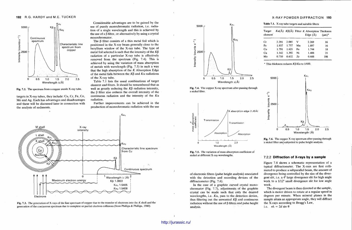
192 R.G. HARDY and M.E. TUCKER
5000
-2500
Continuous spectrum
a K a ,
Characteristic line spectrum from
copper
0.5 1.0 1.5 2.0 Wavelength \(A)
2.5
Fig. 7.2. The spectrum from a copper anode X-ray tube.
targets in X-ray tubes , they include: Cu, Cr , F e , Co , M o and Ag . Each has advantages and disadvantages and these will be discussed later in connection with the analysis of sediments .
Considerable advantages are to be gained by the use of purely monochromat ic radiat ion, i.e. radiation of a single wavelength and this is achieved by the use of a p filter, or alternatively by using a crystal monochromator .
T h e (3 filter consists of a thin metal foil which is positioned in the X-ray beam generally close to the beryllium window of the X-ray tube . T h e type of metal foil selected is such that the intensity of the K$ radiation of a particular X-ray tube is effectively removed from the spectrum (Fig. 7.4). This is achieved by using the variation of mass absorption of metals with wavelength (Fig. 7.5) in such a way that the high absorpt ion of the K Absorpt ion Edge of the metal falls between the K$ and Ka. radiations of the X-ray tube .
Table 7.1 lists the usual combinat ions of target e lement and filters. It should be r emembered that as well as greatly reducing the K$ radiation intensity, the P filter also reduces the overall intensity of the cont inuous Tadiation and the intensity of the Kcc radiat ion.
Fur ther improvements can be achieved in the production of monochromat ic radiation with the use
K a - ]
M shell X-ray
Electrons
Fig. 7.3. The generation of X-rays of the line spectrum of copper due to the transfer of electrons into the K shell and the generation of the continuous spectrum due to complete or partial electron collisions (from Phillips & Phillips, 1980).
X-RAY POWDER DIFFRACTION 193
0 0.5 1.0 1.5 2.0 Wavelength \(A)
Fig. 7.4. The copper X-ray spectrum after passing through a nickel filter.
o Q. C
w O
Transmiss ion
K absorp t ion edge (1.49A)
Transmiss ion
Abso rp t i on
0 1.0 2.0 Wave leng th (A)
Fig. 7.5. The variation of mass absorption coefficient of nickel at different X-ray wavelengths.
of electronic filters (pulse height analysis) associated with the detection and recording devices of the diffractometer (Fig. 7.6).
In the case of a graphite curved crystal monochromator (Fig. 7.7), adjustments of the graphite crystal can be made such that only the desired wavelengths, i.e. Ka, pass to the detection device, thus filtering out the unwanted K§ and continuous radiation without the use of p filters and pulse height analysis.
Table 7.1. X-ray tube targets and suitable filters
Target K<x(k) ATf3(A) Filter K Absorption Thickness element Edge (A) (urn)*
Cr 2.291 2.085 V 2.269 16 Fe 1.937 1.757 Mn 1.897 16 Co 1.791 1.621 Fe 1.744 18 Cu 1.542 1.392 Ni 1.488 21 Mo 0.710 0.632 Zr 0.688 108
This thickness reduces Kfi/Ka to 1/600.
5000
c
o 2500
K a 2
-A, 0.5 1.0 1.5 _ 2.0
Wavelength (A) 2.5
Fig. 7.6. The copper X-ray spectrum after passing through a nickel filter and subjected to pulse height analysis.
7.2.2 Diffraction of X-rays by a sample
Figure 7.8 shows a schematic representat ion of a typical diffractometer. T h e X-rays are first colli-mated to produce a subparallel beam, the amount of divergence being controlled by the size of the divergent slit, i.e. a 4° large divergence slit for high angle work to a 1/12° small divergence slit for low angle work.
The divergent beam is then directed at the sample, which is motor driven to rotate at a regular speed in degrees per minute . When mineral planes in the sample attain an appropr ia te angle, they will diffract the X-rays according to Bragg's Law, i.e. rik = 2d sin 0
K o c i
http://jurassic.ru/
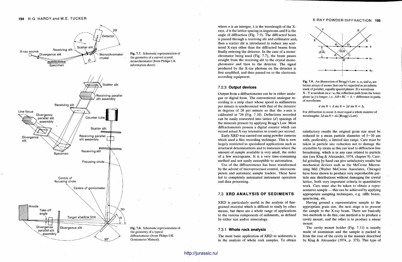
194 R.G. HARDY and M.E. TUCKER
X-ray source Monochromator crystal
Specimen
Fig. 7 . 7 . Schematic representation of the geometry of a curved crystal monochromator (from Philips UK information sheet).
Scatter slit
Receiving parallel slit assembly
o Divergence slit
Specimen Receiving slit
Focusing circle-
Counter tube
Scatter slit
Receiving parallel •—Uf—. slit assembly 1 I
Fig. 7 . 8 . Schematic representation of the geometry of a typical diffractometer (from Philips UK Goniometer Manual).
M l l i l l l
X-RAY POWDER DIFFRACTION 195
where n is an interger, X is the wavelength of the X-rays, d is the lattice spacing in angstroms and 0 is the angle of diffraction (Fig. 7.9). The diffracted beam is passed through a receiving slit and collimator and, then a scatter slit is introduced to reduce any scattered X-rays other than the diffracted beams from finally entering the detector . In the case of a monochromator being used (Fig. 7.7), the beam passes straight from the receiving slit to the crystal monochromator and then to the detector . The signal produced by the X-ray photons on the detector is first amplified, and then passed on to the electronic recording equipment .
7.2.3 Output devices
Outpu t from a diffractometer can be in either analogue or digital form. The conventional analogue recording is a strip chart whose speed in millimetres per minute is synchronized with that of the detector in degrees of 20 per minute so that the x-axis is calibrated in °20 (Fig. 7.10). Deflections recorded can be easily converted into lattice (d) spacings of the minerals present by applying Bragg's Law. Most diffractometers possess a digital counter which can record actual X-ray intensities in counts per second.
Early X R D was carried out using powder cameras which used a film recording technique. This is now largely restricted to specialized applications such as structural determinat ions and to instances where the amount of sample available is very small, the order of a few micrograms. It is a very t ime-consuming method and not easily susceptible to automat ion.
Use of the diffractometer has been transformed by the advent of microprocessor control , microcomputers and automatic sample loaders. These have led to completely au tomated instrument operat ion and data processing.
7.3 X R D A N A L Y S I S OF S E D I M E N T S
X R D is particularly useful in the analysis of finegrained material which is difficult to study by other means , but there are a whole range of applications to the various components of sediments , as defined by either size and/or mineralogy.
7.3.1 Whole rock analysis
The most basic application of X R D to sediments is in the analysis of whole rock samples. To obtain
Fig. 7 .9 . An illustration of Bragg's Law: a, al and a2 are lattice arrays of atoms that can be regarded as an infinite stack of parallel, equally spaced planes. If a wavefront X—Y is incident on a—ax the reflection path from the lower plane ( « i ) is longer, i.e. AB+BC = A = difference in paths of wavefronts
d sin 8 + d sin 6 = 2d sin 9 = A. For diffraction to occur A must equal a whole number of wavelengths: 2d sin 9 = rik (Bragg's Law).
satisfactory results the original grain size must be reduced to a mean particle diameter of 5—10 pm with, preferably, a limited size range. Care must be taken in particle size reduction not to damage the crystallite by strain as this can lead to diffraction line broadening, which is in any case related to particle size (see Klug & Alexander , 1974, chapter 9) . Careful grinding by hand can give satisfactory results but mechanical devices such as the McCrone Micron-izing Mill (Walter McCrone Associates, Chicago) have been shown to produce very reproducible particle size distributions without damaging the crystal lattice, both very important criteria in quantitative work. Care must also be taken to obtain a representative sample — this can be achieved by applying appropria te sampling techniques, e.g. riffle boxes, quar ter ing, etc.
Having ground a representat ive sample to the appropria te grain size, the next stage is to present the sample to the X-ray beam. There are basically two methods to do this; one method is to produce a cavity mount , and the other is to produce a smear mount .
The cavity mount holder (Fig. 7.11) is usually made of aiuminium and the sample is packed in from the rear of the cavity in the manner described by Klug & Alexander (1974, p . 373). This type of
http://jurassic.ru/
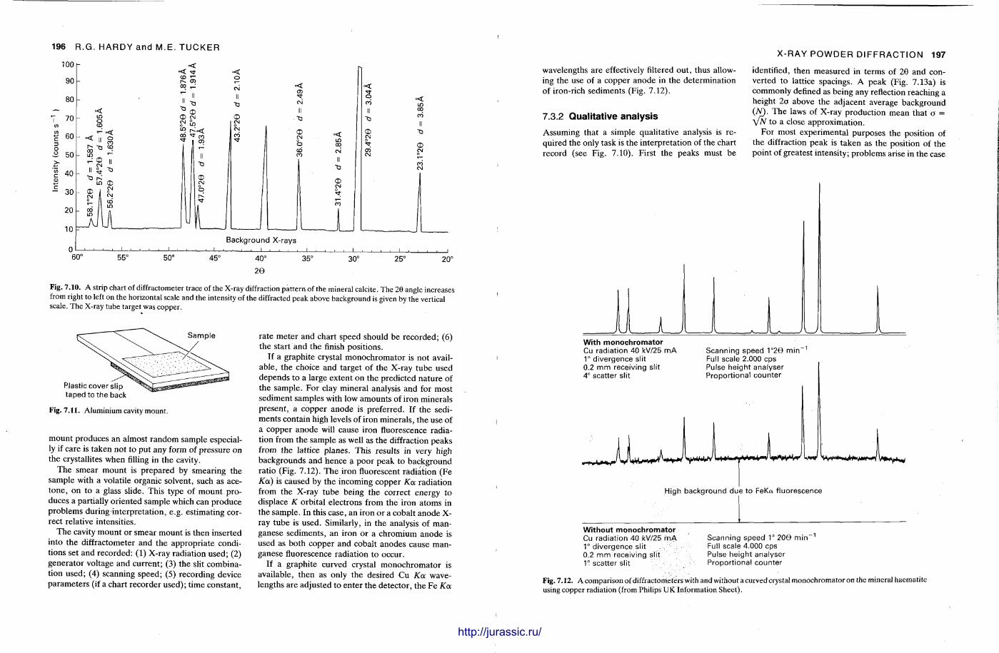
196 R.G. HARDY and M.E. TUCKER
CO
<t> CNJ °° ^r oo
05
< O CD •* C\i CM o O <D ro
Background X-rays
• i i i i i . . . 50° 45° 40° 26
35°
< IS) 00 c\i CD
JL
< o oo
30° 25°
oo
CO
20°
Fig. 7.10. A strip chart of diffractometer trace of the X-ray diffraction pattern of the mineral calcite. The 29 angle increases from right to left on the horizontal scale and the intensity of the diffracted peak above background is given by the vertical scale. The X-ray tube target was copper.
taped to the back
Fig. 7.11. Aluminium cavity mount.
mount produces an almost random sample especially if care is taken not to put any form of pressure on the crystallites when filling in the cavity.
T h e smear moun t is p repared by smear ing the sample with a volatile organic solvent, such as acetone , on to a glass slide. This type of moun t produces a partially or iented sample which can produce problems during interpretat ion, e.g. estimating correct relative intensities.
The cavity mount or smear mount is then inserted into the diffractometer and the appropr ia te condit ions set and recorded: (1) X-ray radiat ion used; (2) generator voltage and current ; (3) the slit combination used; (4) scanning speed; (5) recording device parameters (if a chart recorder used) ; t ime constant ,
rate meter and chart speed should be recorded; (6) t he start and the finish positions.
If a graphite crystal monochromator is not available, the choice and target of the X-ray tube used depends t o a large extent on t he predicted na tu re of the sample . For clay mineral analysis and for most sediment samples with low amounts of iron minerals present , a copper anode is preferred. If the sediments contain high levels of iron minerals , the use of a copper anode will cause iron fluorescence radiation from the sample as well as the diffraction peaks from the lattice planes. This results in very high backgrounds and hence a poor peak to background ratio (Fig. 7.12). The iron fluorescent radiation (Fe Ka) is caused by the incoming copper Ka radiation from the X-ray tube being the correct energy to displace K orbital electrons from the iron atoms in the sample. In this case, an iron or a cobalt anode X-ray tube is used. Similarly, in the analysis of manganese sediments , an iron or a chromium anode is used as bo th copper and cobalt anodes cause manganese fluorescence radiation to occur.
If a graphite curved crystal monochromator is available, then as only the desired Cu Ka wavelengths are adjusted to enter the detector , the Fe Ka
X-RAY POWDER DIFFRACTION 197
wavelengths are effectively filtered out , thus allowing the use of a copper anode in the determinat ion of iron-rich sediments (Fig. 7.12).
7.3.2 Qualitative analysis
Assuming that a simple qualitative analysis is required the only task is the interpretat ion of the chart record (see Fig. 7.10). First the peaks must be
identified, then measured in terms of 26 and converted to lattice spacings. A peak (Fig. 7.13a) is commonly defined as being any reflection reaching a height 2o above the adjacent average background (JV). T h e laws of X-ray product ion mean that o = V'/V to a close approximation.
For most experimental purposes the position of the diffraction peak is taken as the position of the point of greatest intensity; problems arise in the case
j With monochromator Cu radiation 40 kV/25 mA 1° divergence slit 0.2 mm receiving slit 4° scatter slit
Scanning speed 1°26 m i n - 1
Full scale 2.000 cps Pulse height analyser Proportional counter
U High background due to FeKa fluorescence
Without monochromator Cu radiation 40 kV/25 mA 1° divergence slit 0.2 mm receiving slit 1° scatter slit
Scanning speed 1° 200 min Full scale 4.000 cps Pulse height analyser Proportional counter
Fig. 7.12. A comparison of diffractometers with and without a curved crystal monochromator on the mineral haematite using copper radiation (from Philips UK Information Sheet).
http://jurassic.ru/
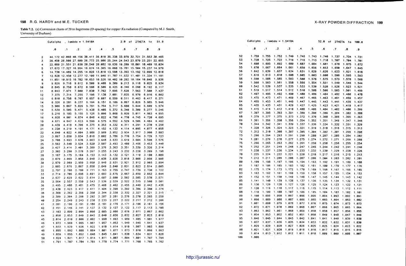
198 R.G. HARDY and M.E. TUCKER
CuKaIpha • I ambda = 1 .5418A 2 . 0 of 2THETA t o 51 . 9
0 1 2 3 4 5 6 7 8 9
2 44 . 172 4 2 . 068 4 0 . 156 3 8 . 411 3 6 . 810 35 338 33 979 32 721 31 553 30 465 3 29 . 450 2 8 . 500 27 . 609 2 6 . 773 2 5 . 986 2 5 . 244 24 543 23 879 23 251 22 655 4 2 2 . 089 21 . 551 21 . 038 20 549 20 082 19 636 19 209 18 801 18 409 18 034 5 17. 673 17. 327 16. 994 16 674 16. 365 16 068 15 781 15 504 15 237 14 979 6 14 . 730 14 . 489 14. 255 14 029 13 810 13 598 13 392 13 192 12 999 12 810 7 12. 628 12 . 450 12. 277 12 109 11 946 11 787 11 632 11 481 11 334 11 191 8 11 . 051 10 . 915 10. 782 10 653 10 526 10 402 10 282 10 164 10 048 9 936 9 9. 826 9 . 718 9 . 612 9 509 9 408 9 309 9 213 9 118 9 025 8 934
18 8 . 845 8 . 758 8 . 672 8 588 8 506 8 425 8 346 8 268 8 192 8 117 11 8 . 043 7 . 971 7. 900 7 830 7 762 7 695 7 628 7 563 7 500 7 437 12 7 375 7 314 7 255 7 196 7 138 7 081 7 025 6 970 6 916 6 862 13 6 810 6 758 6 707 6 657 6 607 6 559 6 511 6 463 6 417 6 371 14 6 326 6 281 6 237 6 194 6 151 6 109 6 067 6 026 5 985 5 946 15 5 906 5 867 5 829 5 791 5 754 5 717 5 680 5 644 5 609 5 574 16 5 539 5 505 5 471 5 438 5 405 5 372 5 340 5 309 5 277 5 246 17 5 216 5 185 5 155 5 126 5 096 5 068 5 039 5 011 4 983 4 955 18 4 928 4 901 4 874 4 848 4 822 4 796 4 770 4 745 4 720 4 695 19 4 671 4 647 4 623 4 599 4 575 4 552 4 529 4 506 4 484 4 462 20 4 439 4 418 4 396 4 375 4 353 4 332 4 311 4 291 4 270 4 250 21 4 230 4 210 4 191 4 171 4 152 4 133 4 114 4 095 4 077 4 058 22 4 040 4 022 4 004 3 986 3 969 3 952 3 934 3 917 3 900 3 883 23 3 867 3 850 3 834 3 818 3 802 3 786 3 770 3 754 3 739 3 723 24 3 708 3 693 3 678 3 663 3 648 3 633 3 619 3 604 3 590 3 576 25 3 562 3 548 3 534 3 520 3 507 3 493 3 480 3 466 3 453 3 440 26 3 427 3 414 3 401 3 389 3 376 3 363 3 351 3 339 3 326 3 314 27 3 302 3 290 3 278 3 267 3 255 3 243 3 232 3 220 3 209 3 198 28 3 187 3 175 3 164 3 153 3 143 3 132 3 121 3 110 3 100 3 089 29 3 079 3 069 3 058 3 048 3 038 3 028 3 018 3 008 2 998 2 988 30 2 979 2 969 2 959 2 950 2 940 2 931 2 921 2 912 2 903 2 894 31 2 885 2 876 2 867 2 858 2 849 2 840 2 831 2 823 2 814 2 805 32 2 .797 2 .788 2 780 2 771 2 763 2 755 2 747 2 739 2 730 2 722 33 2 .714 2 .706 2 698 2 691 2 683 2 675 2 667 2 659 2 652 2 644 34 2 .637 2 .629 2 622 2 614 2 607 2 600 2 592 2 585 2 578 2 571 35 2 .564 2 .557 2 .550 2 .543 2 536 2 529 2 522 2 515 2 508 2 501 36 2 .495 2 .488 2 .481 2 .475 2 468 2 462 2 455 2 449 2 442 2 436 37 2 .430 2 .423 2 .417 2 .411 2 404 2 398 2 392 2 386 2 380 2 374 38 2 .368 2 .362 2 .356 2 .350 2 344 2 338 2 332 2 327 2 321 2 315 39 2 .309 2 .304 2 .298 2 .292 2 287 2 281 2 276 2 270 2 265 2 259 40 2 .254 2 .249 2 .243 2 .238 2 .233 2 .227 2 222 2 217 2 212 2 206 41 2 .201 2 .196 2 .191 2 . 186 2 .181 2 176 2 171 2 166 2 161 2 156 42 2 . 151 2 .146 2 . 141 2 .137 2 .132 2 . 127 2 .122 2 117 2 113 2 108 43 2 .103 2 .099 2 .094 2 .090 2 .085 2 .080 2 .076 2 071 2 067 2 062 44 2 .058 2 .053 2 .049 2 .045 2 .040 2 .036 2 032 2 027 2 023 2 019 45 2 .014 2 .010 2 .006 2 .002 1 .998 1 .993 1 .989 1 985 1 981 1 977 46 1 .973 1 .969 1 .965 1 .961 1 .957 1 .953 1 .949 1 945 1 941 1 937 47 1 .933 1 .929 1 .926 1 .922 1 .918 1 .914 1 910 1 907 1 903 1 899 48 1 .895 1 .892 1 .888 1 .884 1 .881 1 .877 1 .873 1 870 1 866 1 863 49 1 .859 1 .855 1 .852 1 .848 1 .845 1 .841 1 .838 1 834 1 831 1 828 50 1 .824 1 .821 1 .817 1 .814 1 .811 1 .807 1 .804 1 .801 1 797 1 794 51 1 .791 1 .787 1 .784 1 .781 1 .778 1 .774 1 .771 1 .768 1 765 1 762
X-RAY POWDER DIFFRACTION 199
CuKaIpha , lambda = 1.5418A 5 2 . 0 of 2THETA t o 1 0 0 . 0
.1 . 2 . 6 . 9
52 53 54 55 56 57 58 59 60 61 62 63 64 65 66 67 68 69 70 71 72 73 74 75 76 77 78 79 80 81 82 83 84 85 86 87 88 89 90 91 92 93 94 95 96 97 98 99
100
1 .759 1 .728 1 . 698 1 .670 1 .642 1 .616 1 .590 1 .566 1 .542 1 .519 1 .497 1 .475 1 .455 1 .435 1 .415 1 .397 1 .379 1 .361 1 .344 1 .328 1 .312 1 .296 1 .281 1 .266 1 .252 1 .238 1 .225 1 .212 1 .199 1 . 187 1 .175 1 . 163 1 . 152 1 .141 1 .130 1 .120 1 .110 1 . 100 1 . 090 1 .081 1 .072 1 .063 1 .054 1 .046 1 .037 1 .029 1 .021 1 .014 1 .006
1 . 755 1 . 725 1 .695 1 .667 1 .639 1 .613 1 . 588 1 .563 1 .539 1 .517 1 .495 1 .473 1 .453 1 .433 1 . 414 1 .395 1 .377 1 .359 1 .342 1 .326 1 .310 1 .294 1 .279 1 .265 1 .251 1 .237 1 .224 1 .211 1 .198 1 .186 1 .174
1 . 162 151 140 129
1.119 1 .109 1 .099 1 .089 1 .080 1 .071 1 .062 1 .053 1 .045 1 .037 1 .029 1 .021 1 .013
1 .752 1 . 722 1 .692 1 . 6 6 4 1 .637 1 . 610 1 .585 1 .561 1 .537 1 . 514 1 .492 1 .471 1 .451 1 .431 1 . 412 1 . 3 9 3 1 .375 1 . 358 1 .341 1 . 324 1 .308 1 .293 1 .278 1 .263 1 .249 1 .236 1 .222 1 .209 1 .197 1 . 185 1 .173 1.161 1 . 150 1 . 139 1 . 128 1 .118 1 . 108 1 .098 1 .088 1 .079 1 .070 1 .061 1 .052 1 .044 1 .036 1 .028 1 .020 1-.012
1 .749 1 .719 1 .689 1 .661 1 .634 1 .608 1 .583 1 .558 1 .535 1 .512 1 .490 1 .469 1 .449 1 .429 1 .410 1 .391 1 .373 1 .356 1 .339 1 .323 1 .307 1 .291 1 .277 1 .262 1 .248 1 .234 1 .221 1 .208 1 .196 1 .183 1 .172 1 . 160 1 . 149 1 . 138 1 . 127 1.117 1 . 107 1 .097 1 .087 1 .078 1 .069 1 .060 1 .052 1 .043 1 .035 1 .027 1 .019 1 .012
1 . 746 1 . 716 1 .687 1 . 658 1 .631 1 . 605 1 . 580 1 . 556 1 . 5 3 3 1 . 510 1 .488 1 .467 1 .447 1 .427 1 .408 1 .389 1 .372 1 .354 1 .337 1 .321 1 .305 1 .290 1 .275 1 .261 1 .247 1 .233 1 .220 1 .207 1 .194 1 . 182 1 .170 1 .159 1 .148
137 126 116 106
1 .096 1 .086 1 .077 1 .068 1 .059 1 .051 1 .042 1 .034 1 .026 1 .018 1 .011
1 .743 1 . 7 1 3 1 .684 1 .656 1 .629 1 . 6 0 3 1 .578 1 . 554 1 .530 1 . 508 1 .486 1 .465 1 . 445 1 .425 1 .406 1 .388 1 .370 1 .352 1 .336 1 .319 1 . 304 1 .288 1 .274 1 .259 1 .245 1 .232 1 .218 1 .206 1 . 193 1 .181 1 .169 1 .158 1 . 147 1 . 136 1 .125 1.115 1 . 105 1 .095 1 .085 1 .076 1 .067 1 .058 1 .050 1 .041 1 .033 1 .025 1 . 0 1 8 . 1 .010
1 . 740 1 . 710 1 .681 1 .653 1 . 626 1 .600 1 . 575 1 .551 1 . 528 1 .506 1 .484 1 . 4 6 3 1 .443 1 .423 1 . 404 1 . 386 1 . 368 1 .351 1 . 334 1 . 318 1 .302 1 .287 1 .272 1 .258 1 . 244 1 . 230 1 .217 1 .284 1 .192 1 .180 1 .168 1 .157
145 135 124 114
1 .104 1 .094 1 .085 1 .075 1 .066 1 .058 1 .049 1 .041 1 .032 1 .025 1 .017 1 .009
1 .737 1 . 7 0 7 1 . 678 1 . 6 5 0 1 . 6 2 3 1 . 5 9 8 1 . 5 7 3 1 . 549 1 . 526 1 . 5 0 3 1 .482 1 .461 1 .441 1 .421 1 .402 1 . 3 8 4 1 . 366 1 .349 1 .332 1 . 316 1 .301 1 . 285 1 .271 1 . 256 1 .242 1 .229 1 .216 1 . 2 0 3 1 . 191 1 .179 1 .167 1 . 155 1 . 1 4 4 1 . 134 1 . 1 2 3 1 .113 1 . 1 0 3 1 .093 1 . 084 1 .074 1 .065 1 .057 1 .048 1 . 040 1 .032 1 .024 1 . 016 1 .009
1 . 7 3 4 1 . 7 0 4 1 . 6 7 5 1 .647 1 .621 1 . 595 1 . 570 1 .546 1 .523 1 .501 1 . 480 1 .459 1 .439 1 . 419 1 . 400 1 .382 1 .365 1 .347 1 .331 1 .315 1 .299 1 . 284 1 .269 1 .255 1 .241 1 .228 1 .215 1 .202 1 . 189 1 .177 1 .166 1 . 154 1 . 1 4 3 1 . 132 1 . 122 1 .112 1 . 102 1 .092 1 .083 1 .073 1 .065 1 . 056 1 .047 1 .039 1 .031 1 .023 1 .015 1 .008
1 .731 1 .701 1 .672 1 .645 1 . 618 1 . 5 9 3 1 .568 1 .544 1 .521 1 .499 1 . 478 1 .457 1 .437 1 .417 1 .399 1 . 380 1 . 3 6 3 1 . 346 1 . 329 1 .313 1 .298 1 .282 1 . 268 1 .254 1 .240 1 .226 1 .213 1 .201 1 . 188 1 . 176 1 .165 1 .153 1 .142 1 . 131 1 .121 1.111 1 . 101 1 .091 1 .082 1 .073 1 .064 1 .055 1 .046 1 .038 1 .030 1 .022 1 .015 1 .007
i l l l
Table 7.2. (a) Conversion charts of 29 to angstroms (D-spacing) for copper Ka radiation (Computed by M.J. Smith, University of Durham)
http://jurassic.ru/
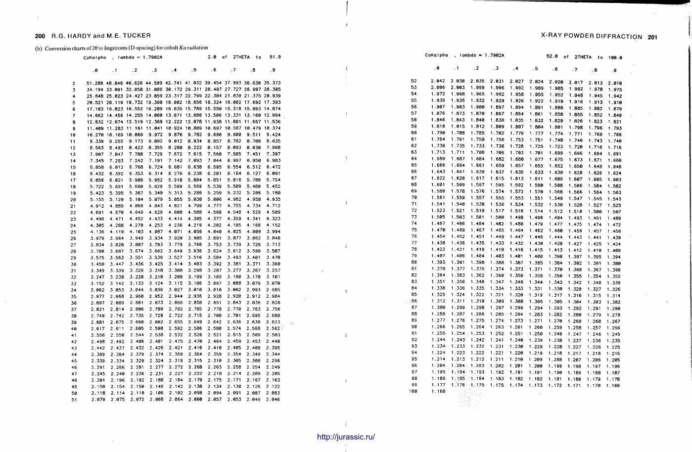
200 R.G. HARDY and M.E. TUCKER X-RAY POWDER DIFFRACTION 201
(b) Conversion charts of 20 to angstroms (D-spacing) for cobalt Ka radiation
CoKalpha , lambda = 1.7902A 2 . 0 of 2THETA t o 5 1 . 9
0 1 2 3 4 5 6 7 8 9
2 51 . 288 4 8 . 846 4 6 . 626 44 599 42 741 41 032 39 454 37 993 36 636 35 373 3 3 4 . 194 3 3 . 091 3 2 . 058 31 086 30 172 29 311 28 497 27 727 26 997 26 305 4 2 5 . 648 25 . 023 2 4 . 427 23 859 23 317 22 799 22 304 21 830 21 375 20 939 5 20 . 521 20 . 119 19 . 732 19 360 19 002 18 656 18 324 18 002 17 692 17 393 6 17. 103 16. 823 16. 552 16 289 16 035 15 789 15 550 15 318 15 093 14 874 7 14. 662 14. 456 14. 255 14 060 13 871 13 686 13 506 13 331 13 160 12 994 8 12 . 832 12 674 12 519 12 369 12 222 12 078 11 938 11 801 11 667 11 536 9 11 . 409 11 283 11 161 11 041 10 924 10 809 10 697 10 587 10 479 10 374
10 10. 270 10 169 10 069 9 972 9 876 9 782 9 690 9 600 9 511 9 424 11 9 . 339 9 255 9 173 9 092 9 012 8 934 8 857 8 782 8 708 8 635 12 8. 563 8 493 8 423 8 355 8 288 8 222 8 157 8 093 8 030 7 968 13 7. 907 7 847 7 788 7 729 7 672 7 615 7 560 7 505 7 451 7 397 14 7 345 7 293 7 242 7 191 7 142 7 093 7 044 6 997 6 950 6 903 15 6 858 6 812 6 768 6 724 6 681 6 638 6 595 6 554 6 512 6 472 16 6 432 6 392 6 353 6 314 6 276 6 238 6 201 6 164 6 127 6 091 17 6 056 6 021 5 986 5 952 5 918 5 884 5 851 5 818 5 786 5 754 18 5 722 5 691 5 660 5 629 5 599 5 569 5 539 5 509 5 480 5 452 19 5 423 5 395 5 367 5 340 5 313 5 286 5 259 5 232 5 206 5 180 20 5 155 5 129 5 104 5 079 5 055 5 030 5 006 4 982 4 958 4 935 21 4 912 4 889 4 866 4 843 4 821 4 799 4 777 4 755 4 734 4 712 22 4 691 4 670 4 649 4 629 4 608 4 588 4 568 4 548 4 529 4 509 23 4 490 4 471 4 452 4 433 4 414 4 395 4 377 4 359 4 341 4 323 24 4 305 4 288 4 270 4 253 4 236 4 219 4 202 4 185 4 168 4 152 25 4 136 4 119 4 103 4 087 4 071 4 056 4 040 4 025 4 009 3 994 26 3 979 3 964 3 949 3 934 3 920 3 905 3 891 3 877 3 862 3 848 27 3 834 3 820 3 807 3 793 3 779 3 766 3 753 3 739 3 726 3 713 28 3 700 3 687 3 674 3 662 3 649 3 636 3 624 3 612 3 599 3 587 29 3 575 3 563 3 551 3 539 3 527 3 516 3 504 3 493 3 481 3 470 30 3 458 3 447 3 436 3 425 3 414 3 403 3 392 3 381 3 371 3 360 31 3 349 3 339 3 329 3 318 3 308 3 298 3 287 3 277 3 267 3 257 32 3 247 3 238 3 228 3 218 3 208 3 199 3 189 3 180 3 170 3 161 33 3 152 3 142 3 133 3 124 3 115 3 106 3 097 3 088 3 079 3 070 34 3 062 3 053 3 044 3 036 3 027 3 018 3 010 3 002 2 993 2 985 35 2 977 2 968 2 960 2 952 2 944 2 936 2 928 2 920 2 912 2 904 36 2 897 2 889 2 881 2 873 2 866 2 858 2 851 2 843 2 836 2 828 37 2 821 2 814 2 806 2 799 2 792 2 785 2 778 2 770 2 763 2 756 38 2 749 2 742 2 735 2 729 2 722 2 715 2 708 2 701 2 695 2 688 39 2 681 2 675 2 668 - 2 662 2 655 2 649 2 642 2 636 2 630 2 623 40 2 617 2 611 2 605 2 598 2 592 2 586 2 580 2 574 2 568 2 562 41 2 .556 2 .550 2 .544 2 .538 2 532 2 526 2 521 2 515 2 509 2 503 42 2 .498 2 .492 2 .486 2 .481 2 475 2 470 2 464 2 459 2 453 2 448 43 2 .442 2 .437 2 .432 2 .426 2 421 2 416 2 410 2 405 2 400 2 395 44 2 .389 2 .384 2 .379 2 .374 2 369 2 364 2 359 2 354 2 349 2 344 45 2 .339 2 .334 2 .329 2 .324 2 319 2 315 2 310 2 305 2 300 2 296 46 2 .291 2 .286 2 .281 2 .277 2 272 2 268 2 263 2 258 2 254 2 249 47 2 .245 2 .240 2 .236 2 .231 2 227 2 222 2 218 2 214 2 209 2 205 48 2 .201 2 .196 2 .192 2 . 188 2 .184 2 179 2 175 2 171 2 167 2 163 49 2 .158 2 .154 2 .150 2 . 146 2 .142 2 138 2 134 2 130 2 126 2 122 50 2 .118 2 . 114 2 .110 2 . 106 2 .102 2 098 2 094 2 091 2 087 2 083 51 2 .079 2 .075 2 .072 2 .068 2 064 2 060 2 057 2 053 2 049 2 046
CoKalpha , Iambda = 1.7902A 5 2 . 0 of 2THETA to 100.
0 1 .2 3 . 4 . 5 . 6 .7 . 8 .9
52 2 042 2 038 2 . 0 3 5 2 031 2 027 2 . 024 2 . 0 2 0 2 .017 2 . 0 1 3 2 .010 53 2 006
CM 003 1 .999 1 .996 1 .992 1 .989 1 . 985 1 .982 1 .978 1 .975 54 1 972 1 968 1 . 965 1 962 1 .958 1 . 955 1 .952 1 .948 1 . 945 1 .942 55 1 939 1 935 1 .932 1 929 1 .926 1 .922 1 .919 1 .916 1 . 9 1 3 1 .910 56 1 907 1 903 1 . 900 1 897 1 894 1 .891 1 . 888 1 . 885 1 .882 1 .879 57 1 876 1 873 1 . 870 1 867 1 864 1 .861 1 . 858 1 .855 1 .852 1 .849 58 1 846 1 843 1 . 840 1 838 1 835 1 .832 1 . 829 1 .826 1 .823 1 .821 59 1 818 1 815 1 . 812 1 809 1 .807 1 .804 1 .801 1 .798 1 .796 1 .793 60 1 790 1 788 1 . 785 1 782 1 .779 1 .777 1 . 774 1 .771 1 .769 1 .766 61 1 764 1 761 1 . 758 1 756 1 753 1 .751 1 . 748 1 .746 1 .743 1 .740 62 1 738 1 735 1 . 7 3 3 1 730 1 728 1 .725 1 . 7 2 3 1 .720 1 .718 1 .716 63 1 713 1 711 1 .708 1 706 1 703 1 .701 1 699 1 .696 1 . 694 1 .691 64 1 689 1 687 1 .684 1 682 1 680 1 .677 1 675 1 .673 1 .671 1 .668 65 1 666 1 664 1 .661 1 659 1 657 1 .655 1 . 652 1 . 650 1 .648 1 .646 66 1 643 1 641 1 .639 1 637 1 635 1 .633 1 630 1 .628 1 .626 1 .624 67 1 622 1 620 1 .617 1 615 1 613 1 611 1 609 1 .607 1 .605 1 .603 68 1 601 1 599 1 .597 1 595 1 592 1 590 1 588 1 .586 1 . 584 1 .582 69 1 580 1 578 1 .576 1 574 1 572 1 570 1 568 1 .566 1 .564 1 .563 70 1 561 1 559 1 .557 1 555 1 553 1 551 1 549 1 .547 1 . 545 1 .543 71 1 541 1 540 1 . 538 1 536 1 534 1 532 1 530 1 528 1 .527 1 .525 72 1 523 1 521 1 .519 1 517 1 516 1 514 1 512 1 510 1 508 1 507 73 1 505 1 503 1 .501 1 500 1 498 1 496 1 494 1 493 1 491 1 489 74 1 487 1 486 1 . 484 1 482 1 480 1 479 1 477 1 475 1 474 1 472 75 1 470 1 469 1 .467 1 465 1 464 1 462 1 460 1 459 1 457 1 456 76 1 454 1 452 1 .451 1 449 1 447 1 446 1 444 1 443 1 441 1 439 77 1 438 1 436 1 .435 1 433 1 432 1 430 1 428 1 427 1 425 1 424 78 1 422 1 421 1 .419 1 418 1 416 1 415 1 413 1 412 1 410 1 409 79 1 407 1 406 1 .404 1 403 1 401 1 400 1 398 1 397 1 395 1 394 80 1 393 1 391 1 . 390 1 388 1 387 1 385 1 384 1 382 1 381 1 380 81 1 378 1 377 1 .375 1 374 1 373 1 371 1 370 1 368 1 367 1 366 82 1 364 1 363 1 .362 1 360 1 359 1 358 1 356 1 355 1 354 1 352 83 1 351 1 350 1 .348 1 347 1 346 1 344 1 343 1 342 1 340 1 339 84 1 338 1 336 1 .335 1 334 1 333 1 331 1 330 1 329 1 327 1 326 85 1 325 1 324 1 .322 1 321 1 320 1 319 1 317 1 316 1 315 1 314 86 1 312 1 311 1 .310 1 309 1 308 1 306 1 305 1 304 1 303 1 302 87 1 300 1 299 1 .298 1 297 1 296 1 294 1 293 1 292 1 291 1 290 88 1 289 1 287 1 . 286 1 285 1 284 1 283 1 282 1 280 1 279 1 278 89 1 277 1 276 1 . 275 1 274 1 273 1 271 1 270 1 269 1 268 1 267 90 1 266 1 265 1 .264 1 263 1 261 1 260 1 259 1 258 1 257 1 256 91 1 255 1 254 1 .253 1 252 1 251 1 250 1 249 1 247 1 246 1 245 92 1 244 1 243 1 .242 1 241 1 240 1 239 1 238 1 237 1 236 1 235 93 1 234 1. 233 1 .232 1 231 1 230 1 229 1 228 1 227 1 226 1 225 94 1 224 1 223 1 .222 1 221 1 220 1 219 1 218 1 217 1 216 1 215 95 1 214 1 213 1 .212 1 211 1 210 1 209 1 208 1 207 1 206 1 . 205 96 1 204 1 204 1 .203 1 202 1 201 1 200 1 199 1 198 1 . 197 1 . 196 97 1 .195 .1 .194 •1 . 193 1 192 1 191 1 191 1 190 1 189 1 188 1 . 187 98 1 .186 t .185 1 ,184 1 183 1 182 1 182 1 181 1 180 1 . 179 1 . 178 99 1 177 1 .'176 1 .175 1 175 1 174 1 173 1 172 1 171 1 . 170 1 . 169
100 1 .168
i
http://jurassic.ru/
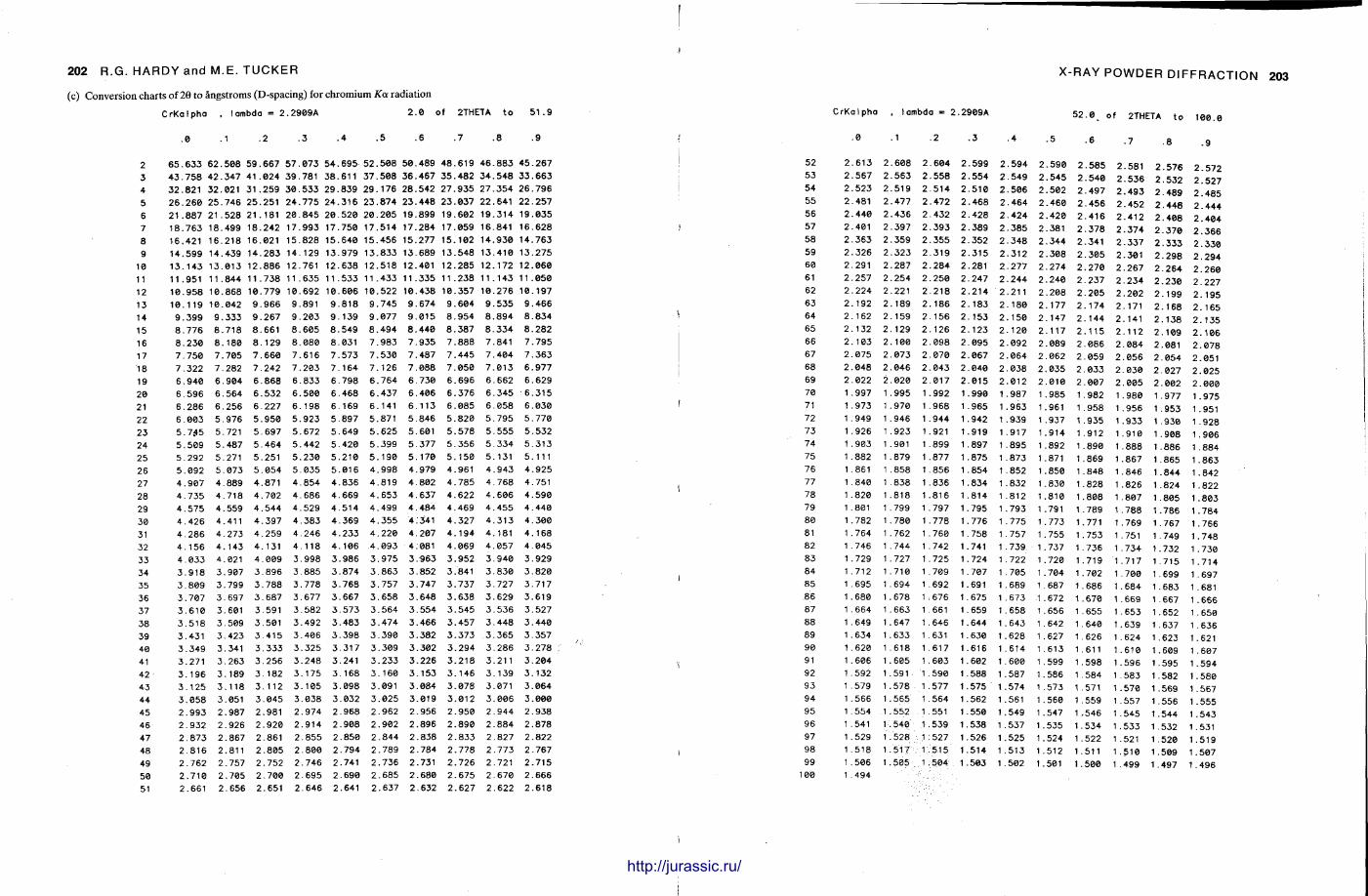
2 0 2 R.G. HARDY and M.E. TUCKER
(c) Conversion charts of 28 to angstroms (D-spacing) for chromium Ka radiation
CrKalpho) • I ambda = 2 .2909A 2 0 o f 2THETA t o 51 . 9
0 1 2 3 4 5 6 7 8 9
2 6 5 . 633 6 2 . 508 5 9 . 667 5 7 . 073 5 4 . 695 5 2 . 508 50 489 48 619 46 883 45 267 3 4 3 . 758 4 2 . 347 41 . 024 3 9 . 781 3 8 . 611 37 . 508 36 467 35 482 34 548 33 663 4 3 2 . 821 3 2 . 021 31 . 259 3 0 . 533 29 . 839 2 9 . 176 28 542 27 935 27 354 26 796 5 2 6 . 260 2 5 . 746 2 5 . 251 2 4 . 775 24 . 316 23 874 23 448 23 037 22 641 22 257 6 21 . 887 21 . 528 21 . 181 20 845 20 520 20 205 19 899 19 602 19 314 19 035 7 18. 763 18. 499 18. 242 17 993 17 750 17 514 17 284 17 059 16 841 16 628 8 16. 421 16. 218 16. 021 15 828 15 640 15 . 456 15 277 15 102 14 930 14 763 9 14 . 599 14. 439 14. 283 14 129 13 979 13 833 13 689 13 548 13 418 13 275
18 13 . 143 13. 013 12. 886 12 761 12 638 12 518 12 401 12 285 12 172 12 860 11 11 . 951 11 . 844 11 . 738 11 635 11 533 11 433 11 335 11 238 11 143 11 050 12 10 . 958 18. 868 10 779 10 692 10 606 10 522 10 438 10 357 10 276 10 197 13 10 . 119 10. 042 9 966 9 891 9 818 9 745 9 674 9 604 9 535 9 466 14 9 . 399 9 . 333 9 267 9 203 9 139 9 077 9 015 8 954 8 894 8 834 15 8 . 776 8 . 718 8 661 8 605 8 549 8 494 8 440 8 387 8 334 8 282 16 8 230 8 180 8 129 8 088 8 031 7 983 7 935 7 888 7 841 7 795 17 7 750 7 705 7 660 7 616 7 573 7 530 7 487 7 445 7 484 7 363 18 7 322 7 282 7 242 7 283 7 164 7 126 7 088 7 050 7 813 6 977 19 6 940 6 904 6 868 6 833 6 798 6 764 6 730 6 696 6 662 6 629 20 6 596 6 564 6 532 6 500 6 468 6 437 6 406 6 376 6 345 6 315 21 6 286 6 256 6 227 6 198 6 169 6 141 6 113 6 085 6 058 6 030 22 6 883 5 976 5 950 5 923 5 897 5 871 5 846 5 820 5 795 5 770 23 5 7.45 5 721 5 697 5 672 5 649 5 625 5 601 5 578 5 555 5 532 24 5 589 5 487 5 464 5 442 5 420 5 399 5 377 5 356 5 334 5 313 25 5 292 5 271 5 251 5 230 5 210 5 190 5 170 5 150 5 131 5 111 26 5 892 5 073 5 054 5 035 5 016 4 998 4 979 4 961 4 943 4 925 27 4 987 4 889 4 871 4 854 4 836 4 819 4 802 4 785 4 768 4 751 28 4 735 4 718 4 702 4 686 4 669 4 653 4 637 4 622 4 606 4 590 29 4 575 4 559 4 544 4 529 4 514 4 499 4 484 4 469 4 455 4 440 30 4 426 4 411 4 397 4 383 4 369 4 355 4 341 4 327 4 313 4 300 31 4 286 4 273 4 259 4 246 4 233 4 220 4 207 4 194 4 181 4 168 32 4 156 4 143 4 131 4 118 4 106 4 093 4 081 4 069 4 057 4 045 33 4 833 4 021 4 009 3 998 3 986 3 975 3 963 3 952 3 940 3 929 34 3 918 3 907 3 896 3 885 3 874 3 863 3 852 3 841 3 830 3 820 35 3 809 3 799 3 788 3 778 3 768 3 757 3 747 3 737 3 727 3 717 36 3 .707 3 .697 3 687 3 677 3 667 3 658 3 648 3 638 3 629 3 619 37 3 .610 3 .601 3 591 3 582 3 573 3 564 3 554 3 545 3 536 3 527 38 3 .518 3 .509 3 501 3 492 3 483 3 474 3 466 3 457 3 448 3 440 39 3 .431 3 .423 3 415 3 406 3 398 3 390 3 382 3 373 3 365 3 357 40 3 .349 3 .341 3 .333 3 .325 3 317 3 309 3 302 3 294 3 286 3 278 41 3 .271 3 .263 3 .256 3 .248 3 241 3 233 3 226 3 218 3 211 3 204 42 3 .196 3 . 189 3 .182 3 .175 3 168 3 160 3 153 3 146 3 139 3 132 43 3 .125 3 .118 3 .112 3 .105 3 098 3 091 3 084 3 078 3 071 3 064 44 3 .058 3 .051 3 .045 3 .038 3 .032 3 025 3 019 3 012 3 086 3 000 45 2 .993 2 .987 2 .981 2 .974 2 .968 2 962 2 956 2 958 2 944 2 938 46 2 .932 2 .926 2 .928 2 .914 2 .908 2 902 2 896 2 890 2 884 2 878 47 2 .873 2 .867 2 .861 2 .855 2 .850 2 .844 2 .838 2 833 2 827 2 822 48 2 .816 2 .811 2 .805 2 .800 2 .794 2 .789 2 .784 2 778 2 773 2 767 49 2 .762 2 .757 2 .752 2 .746 2 .741 2 .736 2 .731 2 726 2 721 2 715 50 2 .710 2 .705 2 .700 2 .695 2 .690 2 .685 2 .680 2 675 2 670 2 666 51 2 .661 2 .656 2 .651 2 .646 2 .641 2 .637 2 .632 2 627 2 622 2 618
.III
I
X-RAY POWDER DIFFRACTION 2 0 3
CrKalpha , lambda = 2.2909A 5 2 . 0 o f 2THETA t o 1
8 1 2 . 3 . 4 . 5 . 6 .7 .8 . 9
52 2 613 2 608 2 604 2 .599 2 . 594 2 .598 2 . 5 8 5 2 .581 2 . 5 7 6 2 . 5 7 2 53 2 567 2 563 2 558 2 . 554 2 .549 2 . 545 2 . 5 4 0 2 . 5 3 6 2 . 5 3 2 2 . 5 2 7 54 2 523 2 519 2 514 2 518 2 .506 2 .502 2 . 4 9 7 2 . 4 9 3 2 . 4 8 9 2 . 4 8 5 55 2 481 2 477 2 472 2 .468 2 .464
CM .460 2 . 4 5 6 2 . 4 5 2 2 . 4 4 8 2 . 4 4 4
56 2 440 2 436 2 432 2 428 2 . 424 2 .420 2 . 4 1 6 2 . 4 1 2 2 . 4 0 8 2 . 4 0 4 57 2 401 2 397 2 393 2 389 2 .385
CM .381 2 . 3 7 8 2 . 3 7 4 2 . 3 7 0 2 . 3 6 6
58 2 363 2 359 2 355 2 352 2 348 2 .344 2 . 3 4 1 2 . 3 3 7 2 . 3 3 3 2 . 3 3 0 59 2 326 2 323 2 319 2 315 2 .312 2 .308 2 . 3 0 5 2 .301 2 . 2 9 8 2 . 2 9 4 68 2 291 2 287 2 284 2 281 2 277 2 .274 2 . 2 7 0 2 . 2 6 7 2 . 2 6 4 2 . 2 6 0 61 2 257 2 254 2 250 2 247 2 244 2 .240 2 . 2 3 7 2 . 2 3 4 2 . 2 3 0 2 . 2 2 7 62 2 224 2 221 2 218 2 214 2 .211 2 .208 2 . 2 0 5 2 . 2 0 2 2 . 1 9 9 2 . 1 9 5 63 2 192 2 189 2 186 2 183 2 180 2 .177 2 . 174 2 . 171 2 . 1 6 8 2 . 165 64 2 162 2 159 2 156 2 153 2 150 2 .147 2 . 144 2 .141 2 . 1 3 8 2 . 135 65 2 132 2 129 2 126 2 123 2 120 2 .117 2 . 1 1 5 2 . 1 1 2 2 . 1 0 9 2 . 1 0 6 66 2 103 2 108 2 098 2 895 2 092 2 .089 2 . 0 8 6 2 . 0 8 4 2 .081 2 . 0 7 8 67 2 075 2 073 2 070 2 067 2 064 2 062 2 . 0 5 9 2 . 0 5 6 2 . 0 5 4 2 .051 68 2 048 2 046 2 043 2 840 2 038 2 835 2 . 0 3 3 2 . 0 3 0 2 . 0 2 7 2 . 0 2 5 69 2 022 2 020 2 017 2 015 2 012 2 010 2 . 0 0 7 2 . 0 0 5 2 . 0 0 2 2 . 0 0 0 78 1 997 1 995 1 992 1 990 1 987 1 985 1 .982 1 .980 1 .977 1 . 975 71 1 973 1 970 1 968 1 965 1 963 1 961 1 .958 1 .956 1 .953 1 .951 72 1 949 1 946 1 944 1 942 1 939 1 937 1 .935 1 .933 1 .930 1 .928 73 1 926 1 923 1 921 1 919 1 917 1 914 1 .912 1 .910 1 .908 1 .906 74 1 903 1 901 1 899 1 897 1 895 1 892 1 .890 1 .888 1 .886 1 .884 75 1 882 1 879 1 877 1 875 1 873 1 871 1 .869 1 .867 1 .865 1 .863 76 1 861 1 858 1 856 1 854 1 852 1 850 1 .848 1 .846 1 .844 1 .842 77 1 840 1 838 1 836 1 834 1 832 1 830 1 .828 1 .826 1 .824 1 .822 78 1 820 1 818 1 816 1 814 1 812 1 810 1 .808 1 .807 1 .805 1 .803 79 1 801 1 799 1 797 1 795 1 793 1 791 1 .789 1 . 788 1 .786 1 .784 80 1 782 1 780 1 778 1 776 1 775 1 773 1 .771 1 .769 1 .767 1 .766 81 1 764 1 762 1 760 1 758 1 757 1 755 1 .753 1 .751 1 .749 1 . 748 82 1 746 1 744 1 742 1 741 1 739 1 737 1 .736 1 .734 1 .732 1 .730 83 1 729 1 727 1 725 1 724 1 722 1 720 1 .719 1 .717 1 .715 1 .714 84 1 712 1 710 1 709 1 707 1 705 1 704 1 .702 1 .700 1 .699 1 .697 85 1 695 1 694 1 692 1 691 1 689 1 687 1 .686 1 .684 1 .683 1 .681 86 1 680 1 678 1 676 1 675 1 673 1 672 1 .670 1 .669 1 .667 1 .666 87 1 664 1 663 1 661 1 659 1 658 1 656 1 .655 1 .653 1 .652 1 .650 88 1 649 1 647 1 646 1 644 1 643 1 642 1 .640 1 .639
1 .637 1 .636 89 1 634 1 633 1 631 1 630 1 628 1 627 1 .626 1 .624 1 .623 1 .621 98 1 620 1 618 1 617 1 616 1 614 1 613 1 .611 1 .610
1 .609 1 .607 91 1 606 1 605 1 603 1 602 1 608 1 599 1 .598 1 .596 1 .595 1 .594 92 1 592 1 591 1 598 1 588 1 587 1 . 586 1 .584 1 .583 1 .582 1 .580 93 1 579 1 578 1 577 1 575 1 574 1 573 1 .571 1 .570
1 .569 1 .567 94 1 566 1 565 1 564 1 562 1 561 1 . 560 1 .559 1 .557 1 .556 1 .555 95 1 554 1 552 1 551 1 550 1 . 549 1 . 547 1 .546 1 .545
1 .544 1 .543 96 1 541 1 5 4 8 1 539 1 538 1 . 537 1 . 535 1 .534 1 .533 1 .532 1 .531 97 1 529 1 5 2 8 1 527 1 526 1 . 525 1 . 524 1 .522 1 .521 1 .520 1 .519 98 1 518 1 51 / 1. 515 1 514 1 . 513 1 . 512 1 .511
1 .510 1 .509 1 .507 99 1 506 1 505 . 1 584 . 1 503 1 . 582 1 . 501 1 .500 1 .499 1 .497 1 .496
100 1 .494
lUUUliUlllllllli I. illllll http://jurassic.ru/
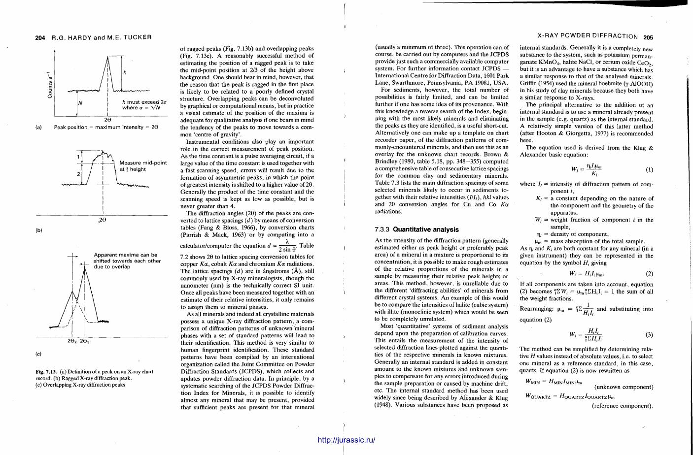
204 R.G. HARDY and M.E. TUCKER
(a) Peak position = maximum intensity = 2 0
Measure mid-point at i height
(b)
.26
Apparent maxima can be shifted towards each other due to overlap
2 6 2 2 0 ,
(c)
Fig. 7.13. (a) Definition of a peak on an X-ray chart record, (b) Ragged X-ray diffraction peak, (c) Overlapping X-ray diffraction peaks.
of ragged peaks (Fig. 7.13b) and overlapping peaks (Fig. 7.13c). A reasonably successful method of estimating the position of a ragged peak is to take the mid-point position at 2/3 of the height above background. One should bear in mind, however, that the reason that the peak is ragged in the first place is likely to be related to a poorly defined crystal s tructure. Overlapping peaks can be deconvoluted by graphical or computat ional means , but in practice a visual est imate of the position of the maxima is adequate for qualitative analysis if one bears in mind the tendency of the peaks to move towards a common 'centre of gravity' .
Ins t rumental conditions also play an impor tant role in the correct measurement of peak position. As the t ime constant is a pulse averaging circuit, if a large value of the time constant is used together with a fast scanning speed, errors will result due to t he formation of asymmetric peaks , in which the point of greatest intensity is shifted t o a higher value of 20 . Generally the product of the t ime constant and the scanning speed is kept as low as possible, but is never greater than 4.
T h e diffraction angles (20) of the peaks are converted to lattice spacings (d) by means of conversion tables (Fang & Bloss, 1966), by conversion charts (Parrish & Mack, 1963) or by computing into a
X calculator/computer the equat ion d = — — - . Table
n 2 sin 0 7.2 shows 20 to lattice spacing conversion tables for copper Koc, cobalt Ka and chromium Ka radiat ions. T h e lattice spacings (d) a re in angstroms (A), still commonly used by X-ray mineralogists, though the nanometer (nm) is the technically correct SI unit. Once all peaks have been measured together with an est imate of their relative intensities, it only remains to assign them to mineral phases .
As all minerals and indeed all crystalline materials possess a un ique X-ray diffraction pa t te rn , a comparison of diffraction pat terns of unknown mineral phases with a set of s tandard pat terns will lead to their identification. This method is very similar to human fingerprint identification. These s tandard pat terns have been compiled by an international organization called the Joint Commit tee on Powder Diffraction Standards ( JCPDS) , which collects and updates powder diffraction data . In principle, by a systematic searching of the J C P D S Powder Diffraction Index for Minerals , it is possible to identify almost any mineral that may be present , provided that sufficient peaks are present for that mineral
X-RAY POWDER DIFFRACTION 205
(usually a minimum of th ree ) . This operat ion can of course, be carried out by computers and the J C P D S provide just such a commercially available computer system. For further information contact J C P D S — Internat ional Cent re for Diffraction Da ta , 1601 Park Lane , Swar thmore , Pennsylvania, P A 19081, U S A .
For sediments , however , the total number of possibilities is fairly limited, and can be limited further if one has some idea of its provenance. With this knowledge a reverse search of the Index, beginning with the most likely minerals and eliminating the peaks as they are identified, is a useful short-cut. Alternatively one can make up a template on chart recorder paper , of the diffraction pat terns of commonly-encountered minerals , and then use this as an overlay for the unknown chart records. Brown & Brindley (1980, table 5.18, pp . 3 4 8 - 3 5 5 ) computed a comprehensive table of consecutive lattice spacings for the common clay and sedimentary minerals. Table 7.3 lists the main diffraction spacings of some selected minerals likely to occur in sediments together with their relative intensities ( / / / , ) , hkl values and 20 conversion angles for Cu and Co Ka radiat ions.
7.3.3 Quantitative analysis
As the intensity of the diffraction pat tern (generally est imated either as peak height or preferably peak area) of a mineral in a mixture is proport ional to its concentrat ion, it is possible to make rough estimates of the relative proport ions of the minerals in a sample by measuring their relative peak heights or areas. This me thod , however , is unreliable due to the different 'diffracting abilities' of minerals from different crystal systems. A n example of this would be to compare the intensities of halite (cubic system) with illite (monoclinic system) which would be seen to be completely unre la ted .
Most 'quant i ta t ive ' systems of sediment analysis depend upon the prepara t ion of calibration curves. This entails the measurement of the intensity of selected diffraction lines plot ted against the quantities of the respective minerals in known mixtures. Generally an internal s tandard is added in constant amount to the known mixtures and unknown samples to compensate for any errors introduced during the sample preparat ion or caused by machine drift, etc . T h e internal s tandard method has been used widely since being described by Alexander & Klug (1948). Various substances have been proposed as
internal s tandards . General ly it is a completely new substance to the system, such as potassium permanganate K M n 0 4 , halite NaCl , or cerium oxide C e 0 2 , but it is an advantage to have a substance which has a similar response to that of the analysed minerals. Griffin (1954) used the mineral boehmite (y-AlOOH) in his study of clay minerals because they both have a similar response to X-rays.
The principal alternative to the addition of an internal s tandard is to use a mineral already present in the sample (e.g. quartz) as the internal s tandard. A relatively simple version of this latter method (after H o o t o n & Giorget ta , 1977) is recommended here .
The equat ion used is derived from the Klug & Alexander basic equat ion:
W, = T),7,p„ K; (1)
where = intensity of diffraction pat tern of componen t i,
Kj = a constant depending on the na ture of the component and the geometry of the appara tus ,
W; = weight fraction of component i in the sample,
r), = density of component , Pn, = mass absorption of the total sample.
As T), and Kt a re both constant for any mineral (in a given instrument) they can be represented in the equat ion by the symbol Ht giving
(2)
If all components are taken into account, equat ion (2) becomes 1LWt = u ^ E F L I i = 1 the sum of all the weight fractions.
Rearranging: ^ = " E r r y and substituting into in
equat ion (2)
w. = H i I i (3)
T h e method can be simplified by determining relative H values instead of absolute values, i.e. to select one mineral as a reference s tandard, in this case, quartz . If equat ion (2) is now rewritten as
W M I N = ^ M I N ^ M I N M T H
(unknown component )
^QUARTZ = ^QUARTZ ̂ QUARTZ Mm
(reference component ) .
l l l i i l http://jurassic.ru/
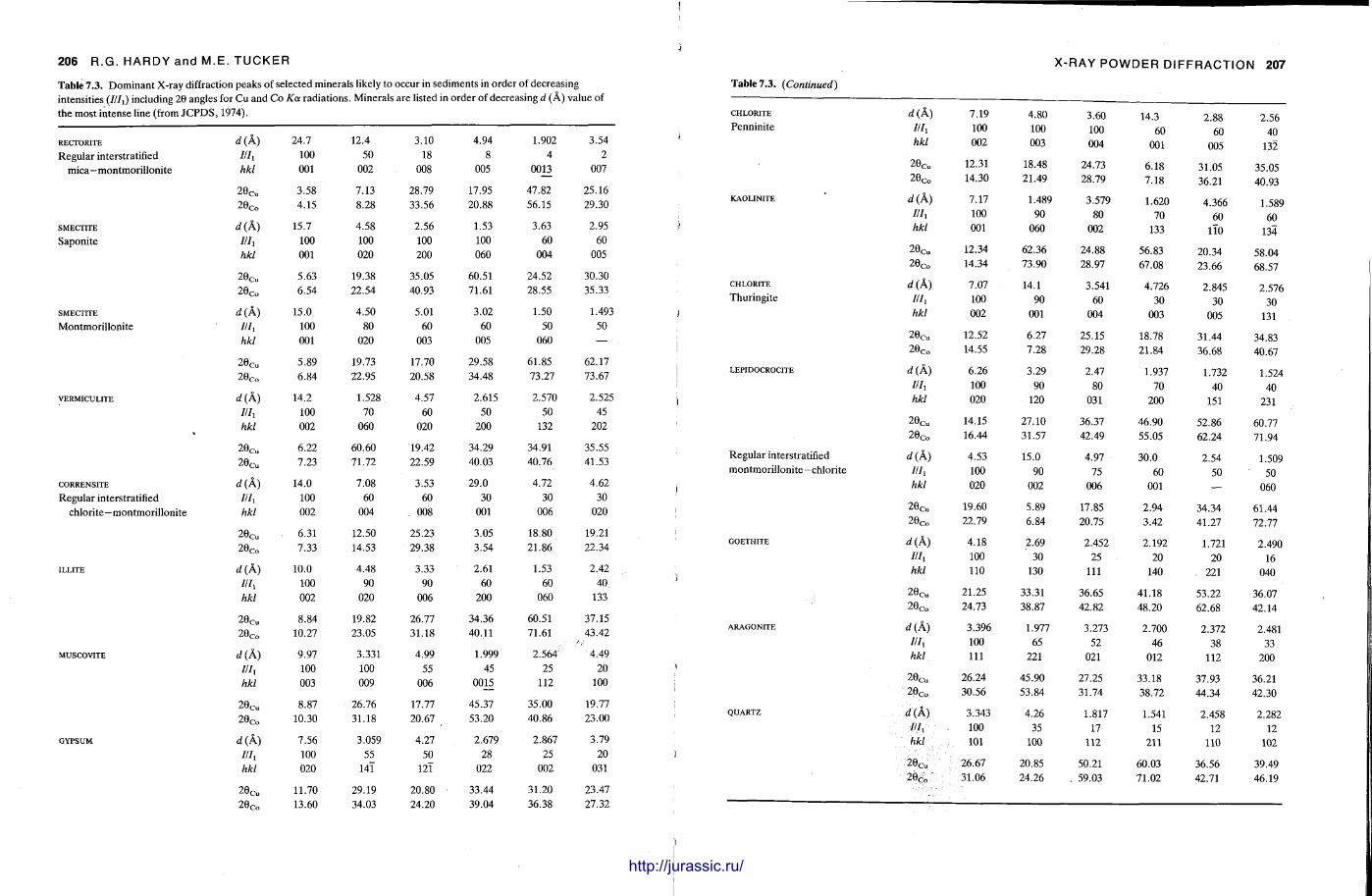
206 R.G. HARDY and M.E. TUCKER
Table 7.3. Dominant X-ray diffraction peaks of selected minerals likely to occur in sediments in order of decreasing intensities (I/h) including 26 angles for Cu and Co Ka radiations. Minerals are listed in order of decreasing d (A) value of the most intense line (from JCPDS, 1974).
RECTORITE d(k) 24.7 12.4 3.10 4.94 1.902 3.54 Regular interstratified Ilh 100 50 18 8 4 2
mica - montmorillonite hkl 001 002 008 005 0013 007
2 6 C u 3.58 7.13 28.79 17.95 47.82 25.16
26c„ 4.15 8.28 33.56 20.88 56.15 29.30
SMECTITE d(k) 15.7 4.58 2.56 1.53 3.63 2.95 Saponite Vh 100 100 100 100 60 60
hkl 001 020 200 060 004 005
2 0 C u 5.63 19.38 35.05 60.51 24.52 30.30 2 6 C o 6.54 22.54 40.93 71.61 28.55 35.33
SMECTITE d(k) 15.0 4.50 5.01 3.02 1.50 1.493 Montmorillonite Hh 100 80 60 60 50 50
hkl 001 020 003 005 060 —
2 6 C u 5.89 19.73 17.70 29.58 61.85 62.17
2 6 C o 6.84 22.95 20.58 34.48 73.27 73.67
VERMICULITE d(A) 14.2 1.528 4.57 2.615 2.570 2.525 I'h 100 70 60 50 50 45 hkl 002 060 020 200 132 202
2 6 C u 6.22 60.60 19.42 34.29 34.91 35.55 2 6 C u
7.23 71.72 22.59 40.03 40.76 41.53
CORRENSITE d(k) 14.0 7.08 3.53 29.0 4.72 4.62 Regular interstratified Hh 100 60 60 30 30 30
chlorite—montmorillonite hkl 002 004 008 001 006 020
26C u 6.31 12.50 25.23 3.05 18.80 19.21
26C o 7.33 14.53 29.38 3.54 21.86 22.34
ILLITE d (A) 10.0 4.48 3.33 2.61 1.53 2.42
Hh 100 90 90 60 60 40 hkl 002 020 006 200 060 133
29cu 8.84 19.82 26.77 34.36 60.51 37.15 26Co 10.27 23.05 31.18 40.11 71.61 43.42
MUSCOVITE d(A) 9.97 3.331 4.99 1.999 2.564 4.49
Hh 100 100 55 45 25 20 hkl 003 009 006 0015 112 100
2 6 C u 8.87 26.76 17.77 45.37 35.00 19.77 2eC o
10.30 31.18 20.67 53.20 40.86 23.00
GYPSUM d (A) 7.56 3.059 4.27 2.679 2.867 3.79
Hh 100 55 50 28 25 20 hkl 020 141 121 022 002 031
2 6 C u 11.70 29.19 20.80 33.44 31.20 23.47
26 c „ 13.60 34.03 24.20 39.04 36.38 27.32
X-RAY POWDER DIFFRACTION 207 Table 7.3. (Continued)
CHLORITE d(k) 7.19 Penninite Hh 100
hkl 002
2 0 C u 12.31
26Co 14.30
KAOLINITE d(k) 7.17 Hh 100 hkl 001
26 c „ 12.34 2 6 C o 14.34
CHLORITE d(k) 7.07 Thuringite Hh 100
hkl 002
2eC u 12.52 2 6 C o
14.55
LEPIDOCROCITE d(k) 6.26 Hh 100 hkl 020
26 c „ 14.15 26 c „ 16.44
Regular interstratified d(k) 4.53 montmorillonite - chlorite Hh 100
hkl 020
2 6 C u 19.60
2 6 C o 22.79
GOETHITE d(k) 4.18 Hh 100 hkl 110
26 c „ 21.25 2 6 C o
24.73
ARAGONITE d(k) 3.396 Hh 100 hkl 111
2 6 C u 26.24
2 6 C o 30.56
QUARTZ d(k) 3.343 : Hh 100
hkl 101
20c-„ ;• 26.67 20<„ 31.06
4.80 3.60 14.3 2.88 2.56 100 100 60 60 40 003 004 001 005 132
18.48 24.73 6.18 31.05 35.05 21.49 28.79 7.18 36.21 40.93
1.489 3.579 1.620 4.366 1.589 90 80 70 60 60
060 002 133 110 134
62.36 24.88 56.83 20.34 58.04 73.90 28.97 67.08 23.66 68.57
14.1 3.541 4.726 2.845 2.576 90 60 30 30 30
001 004 003 005 131
6.27 25.15 18.78 31.44 34.83 7.28 29.28 21.84 36.68 40.67
3.29 2.47 1.937 1.732 1.524 90 80 70 40 40
120 031 200 151 231
27.10 36.37 46.90 52.86 60.77 31.57 42.49 55.05 62.24 71.94
15.0 4.97 30.0 2.54 1.509 90 75 60 50 50
002 006 001 — 060
5.89 17.85 2.94 34.34 61.44 6.84 20.75 3.42 41.27 72.77
2.69 2.452 2.192 1.721 2.490 30 25 20 20 16
130 111 140 221 040
33.31 36.65 41.18 53.22 36.07 38.87 42.82 48.20 62.68 42.14
1.977 3.273 2.700 2.372 2.481 65 52 46 38 33
221 021 012 112 200
45.90 27.25 33.18 37.93 36.21 53.84 31.74 38.72 44.34 42.30
4.26 1.817 1.541 2.458 2.282 35 17 15 12 12
100 112 211 110 102
20.85 50.21 60.03 36.56 39.49 24.26 . 59.03 71.02 42.71 46.19
1 1 1 http://jurassic.ru/
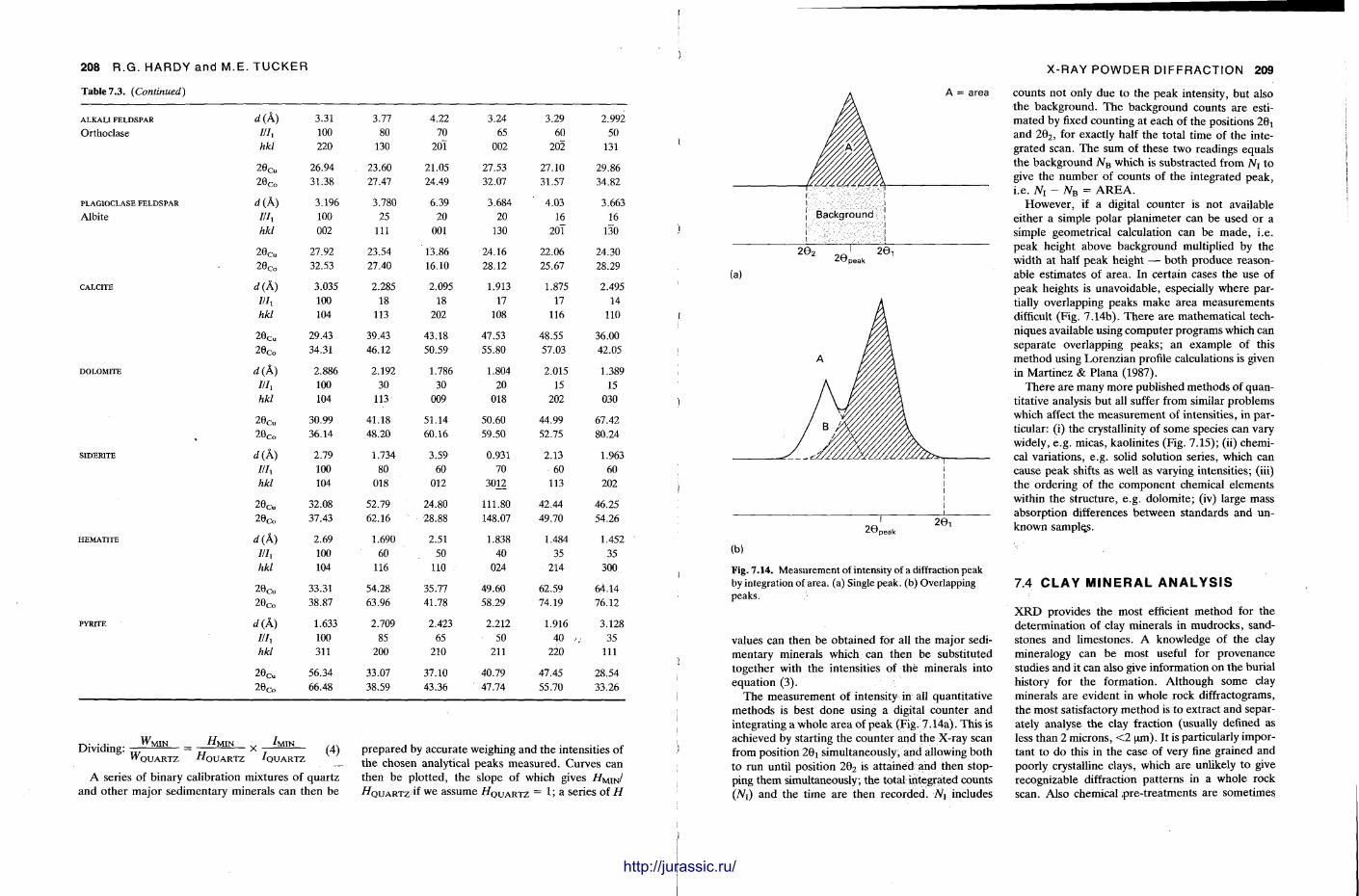
208 R.G. HARDY and M.E. TUCKER
Table 7.3. (Continued)
ALKALI FELDSPAR d(A) 3.31 Orthoclase ilh 100
hkl 220
2 6 C u 26.94 2 6 C o
31.38
PLAGIOCLASE FELDSPAR d(A) 3.196 Albite Hh 100
hkl 002
2 0 C u 27.92
26co 32.53
CALCITE d(A) 3.035 Illi 100 hkl 104
2 6 C u 29.43
2 6 C o 34.31
DOLOMITE d(A) 2.886 ///, 100 hkl 104
2G C u 30.99
2 6 C o 36.14
SIDERITE d(A) 2.79 Ilh 100 hkl 104
26 c „ 32.08 2 6 C o 37.43
HEMATITE d(k) 2.69 llh 100 hkl 104
29cu 33.31 2 6 C o 38.87
PYRITE d(A) 1.633 Ilh 100 hkl 311
2 6 C u 56.34
2 8 C o 66.48
3.77 4.22 3.24 3.29 2.992 80 70 65 60 50
130 201 002 202 131
23.60 21.05 27.53 27.10 29.86 27.47 24.49 32.07 31.57 34.82
3.780 6.39 3.684 4.03 3.663 25 20 20 16 16
111 001 130 201 130
23.54 13.86 24.16 22.06 24.30 27.40 16.10 28.12 25.67 28.29
2.285 2.095 1.913 1.875 2.495 18 18 17 17 14
113 202 108 116 110
39.43 43.18 47.53 48.55 36.00 46.12 50.59 55.80 57.03 42.05
2.192 1.786 1.804 2.015 1.389 30 30 20 15 15
CO 009 018 202 030
41.18 51.14 50.60 44.99 67.42 48.20 60.16 59.50 52.75 80.24
1.734 3.59 0.931 2.13 1.963 80 60 70 60 60
018 012 3012 113 202
52.79 24.80 111.80 42.44 46.25 62.16 28.88 148.07 49.70 54.26
1.690 2.51 1.838 1.484 1.452 60 50 40 35 35
116 110 024 214 300
54.28 35.77 49.60 62.59 64.14 63.96 41.78 58.29 74.19 76.12
2.709 2.423 2.212 1.916 3.128 85 65 50 40 ,.. 35
200 210 211 220 111
33.07 37.10 40.79 47.45 28.54 38.59 43.36 47.74 55.70 33.26
Dividing: MIN ' M I N
Q U A R T Z Hi Q U A R T Z 1 Q U A R T Z (4)
A series of binary calibration mixtures of quar tz and other major sedimentary minerals can then be
prepared by accurate weighing and the intensities of the chosen analytical peaks measured . Curves can then be plot ted, the slope of which gives / / M I N / ^ Q U A R T Z if we assume / / Q U A R T Z = 1; a series of H
11 m m i i f mill
X-RAY POWDER DIFFRACTION 209
A = area
201 ~J~ 207 20 peak
(a)
peak
(b)
Fig. 7.14. Measurement of intensity of a diffraction peak by integration of area, (a) Single peak, (b) Overlapping peaks.
values can then be obtained for all the major sedimentary minerals which can then be substituted together with the intensities of the minerals into equat ion (3).
The measurement of intensity in all quantitative methods is best done using a digital counter and integrating a whole area of peak (Fig.-7.14a). This is achieved by starting the counter and the X-ray scan from position 2 0 t s i m u l t a n e o u s ^ and allowing both to run until position 2 0 2 is at tained and then stopping them simultaneously; the total integrated counts (N{) and the t ime are then recorded. Nt includes
counts not only due to the peak intensity, but also the background. T h e background counts are estimated by fixed counting at each of the positions 20 ! and 2 0 2 , for exactly half the total t ime of the integrated scan. T h e sum of these two readings equals the background NB which is substracted from JVr to give the number of counts of the integrated peak, i .e. NT- 7VB = A R E A .
However , if a digital counter is not available either a simple polar planimeter can be used or a simple geometrical calculation can be made , i.e. peak height above background multiplied by the width at half peak height — both produce reasonable estimates of area. In certain cases the use of peak heights is unavoidable , especially where partially overlapping peaks m a k e area measurements difficult (Fig. 7.14b). T h e r e are mathematical techniques available using computer programs which can separate overlapping peaks ; an example of this me thod using Lorenzian profile calculations is given in Mart inez & Plana (1987).
The re are many more published methods of quantitative analysis but all suffer from similar problems which affect the measurement of intensities, in particular: (i) the crystallinity of some species can vary widely, e.g. micas, kaolinites (Fig. 7.15); (ii) chemical variations, e.g. solid solution series, which can cause peak shifts as well as varying intensities; (iii) the ordering of the component chemical elements within the structure, e.g. dolomite; (iv) large mass absorption differences between standards and unknown samplers.
7.4 C L A Y M I N E R A L A N A L Y S I S
X R D provides the most efficient method for the determinat ion of clay minerals in mudrocks , sandstones and l imestones. A knowledge of the clay mineralogy can be most useful for provenance studies and it can also give information on the burial history for the formation. Al though some clay minerals are evident in whole rock diffractograms, the most satisfactory method is to extract and separately analyse the clay fraction (usually defined as less than 2 microns, < 2 urn). It is particularly important to do this in the case of very fine grained and poorly crystalline clays, which are unlikely to give recognizable diffraction pat terns in a whole rock scan. Also chemical p re - t rea tments are sometimes
http://jurassic.ru/
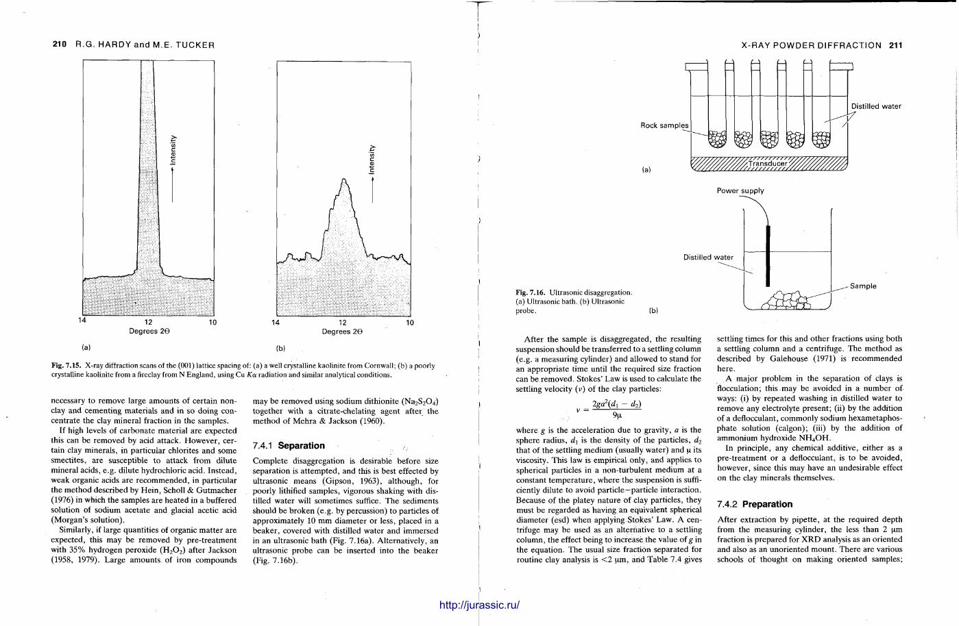
210 R.G. HARDY and M.E. TUCKER
12 Degrees 2G
12 Degrees 26
(a) (b)
Fig. 7.15. X-ray diffraction scans of the (001) lattice spacing of: (a) a well crystalline kaolinite from Cornwall; (b) a poorly crystalline kaolinite from a fireclay from N England, using Cu Ka radiation and similar analytical conditions.
necessary to remove large amounts of certain non-clay and cementing materials and in so doing concentrate the clay mineral fraction in the samples.
If high levels of carbonate material are expected this can be removed by acid attack. However , certain clay minerals , in particular chlorites and some smectites, are susceptible to attack from dilute mineral acids, e.g. dilute hydrochloric acid. Instead, weak organic acids are recommended , in particular the method described by Hein , Scholl & Gutmacher (1976) in which the samples are heated in a buffered solution of sodium acetate and glacial acetic acid (Morgan 's solution).
Similarly, if large quanti t ies of organic mat ter are expected, this may be removed by pre- t rea tment with 3 5 % hydrogen peroxide ( H 2 0 2 ) after Jackson (1958, 1979). Large amounts , of iron compounds
may be removed using sodium dithionite ( N a 2 S 2 0 4 ) together with a citrate-chelating agent after the method of Mehra & Jackson (1960).
7.4.1 Separation
Comple te disaggregation is desirable before size separation is a t tempted , and this is best effected by ultrasonic means (Gipson, 1963), al though, for poorly lithified samples, vigorous shaking with distilled water will sometimes suffice. The sediments should be broken (e.g. by percussion) to particles of approximately 10 m m diameter or less, placed in a beaker , covered with distilled water and immersed in an ultrasonic bath (Fig. 7.16a). Alternatively, an ultrasonic probe can be inserted into the beaker (Fig. 7.16b).
11J11111I11111111
X-RAY POWDER DIFFRACTION 211
Rock samples
(a)
Distilled water
^Jransd^ucer^,
Power supply
Distilled water
Fig. 7.16. Ultrasonic disaggregation, (a) Ultrasonic bath, (b) Ultrasonic probe. (b)
Sample
After the sample is disaggregated, the resulting suspension should be transferred to a settling column (e.g. a measuring cylinder) and allowed to stand for an appropr ia te t ime until the required size fraction can be removed. Stokes ' Law is used to calculate the settling velocity (i>) of the clay particles:
2ga\dx - d2)
; V = % where g is the acceleration due to gravity, a is the sphere radius, d1 is the density of the particles, d2
that of the settling medium (usually water) and u, its viscosity. This law is empirical only, and applies to spherical particles in a non-turbulent medium at a constant t empera tu re , where the suspension is sufficiently dilute to avoid particle—particle interaction. Because of the platey na ture of clay particles, they must be regarded as having an equivalent spherical d iameter (esd) when applying Stokes ' Law. A centrifuge may be used as an alternative to a settling column, the effect being to increase the value of g in the equat ion. The usual size fraction separated for routine clay analysis is < 2 um, and Table 7.4 gives
settling t imes for this and other fractions using both a settling column and a centrifuge. The method as described by Galehouse (1971) is recommended here .
A major problem in the separation of clays is flocculation; this may be avoided in a number of ways: (i) by repeated washing in distilled water to remove any electrolyte present ; (ii) by the addition of a deflocculant, commonly sodium hexametaphospha te solution (calgon); (iii) by the addition of ammonium hydroxide N H 4 O H .
In principle, any chemical additive, either as a pre- t reatment or a deflocculant, is to be avoided, however , since this may have an undesirable effect on the clay minerals themselves.
7.4.2 Preparation
After extraction by pipet te , at the required depth from the measuring cylinder, the less than 2 um fraction is prepared for X R D analysis as an oriented and also as an unor iented mount . There are various schools of thought on making oriented samples;
http://jurassic.ru/
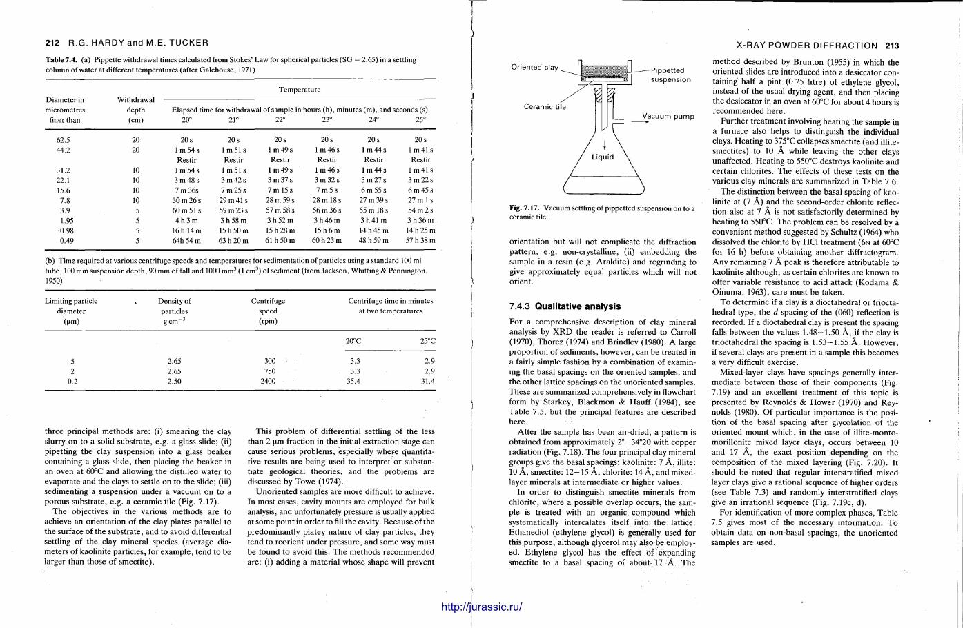
212 R.G. HARDY and M.E. TUCKER
Table 7.4. (a) Pippette withdrawal times calculated from Stokes' Law for spherical particles (SG = 2.65) in a settling column of water at different temperatures (after Galehouse, 1971)
Temperature Diameter in Withdrawal micrometres depth Elapsed time for withdrawal of sample in hours (h), minutes (m), and seconds (s)
finer than (cm) 20° 21° 22° 23° 24° 25°
62.5 20 20 s 20 s 20 s 20 s 20 s 20 s 44.2 20 1 m 54 s l m 5 1 s 1 m49s 1 m46s 1 m44s 1 m41 s
Restir Restir Restir Restir Restir Restir 31.2 10 1 m 54 s 1 m 51 s 1 m 49 s 1 m46s 1 m44s 1 m41 s 22.1 10 3 m 48 s 3 m 42 s 3 m 37 s 3 m 32 s 3 m 27 s 3 m 22 s 15.6 10 7 m 36s 7 m 25 s 7 m 15 s 7 m 5 s 6 m 55 s 6 m 45 s 7.8 10 30 m 26 s 29 m 41 s 28 m 59 s 28 m 18 s 27 m 39 s 27m I s 3.9 5 60 m 51s 59 m 23 s 57 m 58 s 56 m 36 s 55 m 18 s 54 m 2s 1.95 5 4 h 3 m 3 h 5 8 m 3 h 5 2 m 3 h 4 6 m 3h41 m 3 h 3 6 m 0.98 5 16 h 14 m 15 h 50 m 15 h 28 m 15h6m 14 h 45 m 14 h 25 m 0.49 5 64h 54 m 63 h 20 m 61 h 50 m 60 h 23 m 48 h 59 m 57 h 38 m
(b) Time required at various centrifuge speeds and temperatures for sedimentation of particles using a standard 100 ml tube, 100 mm suspension depth, 90 mm of fall and 1000 mm 3 (1 cm 3) of sediment (from Jackson, Whitting & Pennington, 1950)
Limiting particle Density of Centrifuge Centrifuge time in minutes diameter particles speed at two temperatures
(um) g e m " 3 (rpm)
20°C 25°C
5 2.65 300 3.3 2.9 2 2.65 750 3.3 2.9
0.2 2.50 2400 35.4 31.4
three principal methods are: (i) smearing the clay slurry on to a solid substrate , e.g. a glass slide; (ii) pipetting the clay suspension into a glass beaker containing a glass slide, then placing the beaker in an oven at 60°C and allowing the distilled water to evaporate and the clays to settle on to the slide; (iii) sedimenting a suspension under a vacuum on to a porous substrate , e.g. a ceramic tile (Fig. 7.17).
The objectives in the various methods are to achieve an orientat ion of the clay plates parallel to the surface of the substrate , and to avoid differential settling of the clay mineral species (average diameters of kaolinite particles, for example, tend to be larger than those of smecti te) .
This problem of differential settling of the less than 2 urn fraction in the initial extraction stage can cause serious problems, especially where quanti tative results are being used to interpret or substantiate geological theories , and the problems are discussed by T o we (1974).
Unor iented samples are more difficult to achieve. In most cases, cavity mounts are employed for bulk analysis, and unfortunately pressure is usually applied at some point in order to fill the cavity. Because of the predominant ly platey na ture of clay particles, they tend to reorient under pressure, and some way must be found to avoid this. T h e methods recommended are: (i) adding a material whose shape will prevent
X-RAY POWDER DIFFRACTION 213
Oriented clay
Ceramic tile
Pippetted suspension
Vacuum pump
Fig. 7.17. Vacuum settling of pippetted suspension on to a ceramic tile.
orientat ion but will not complicate the diffraction pa t te rn , e.g. non-crystalline; (ii) embedding the sample in a resin (e.g. Araldi te) and regrinding to give approximately equal particles which will not orient.
7.4.3 Qualitative analysis
For a comprehensive description of clay mineral analysis by X R D the reader is referred to Carroll (1970), Thorez (1974) and Brindley (1980). A large propor t ion of sediments , however , can be treated in a fairly simple fashion by a combinat ion of examining the basal spacings on the oriented samples, and the other lattice spacings on the unoriented samples. These are summarized comprehensively in flowchart form by Starkey, Blackmon & Hauff (1984), see Table 7.5, but the principal features are described here .
After the sample has been air-dried, a pat tern is obtained from approximately 2°—34°20 with copper radiation (Fig. 7.18). The four principal clay mineral groups give the basal spacings: kaolinite: 7 A , illite: 10 A , smectite: 12—15 A , chlorite: 14 A , and mixed-layer minerals at in termediate or higher values.
In order to distinguish smectite minerals from chlorite, where a possible overlap occurs, the sample is t reated with an organic compound which systematically intercalates itself into the lattice. Ethanediol (ethylene glycol) is generally used for this purpose , al though glycerol may also be employed. Ethylene glycol has the effect of expanding smectite to a basal spacing of about -17 A . The
method described by Brunton (1955) in which the oriented slides are introduced into a desiccator containing half a pint (0.25 litre) of ethylene glycol, instead of the usual drying agent , and then placing the desiccator in an oven at 60°C for about 4 hours is recommended here .
Fur ther t rea tment involving heating the sample in a furnace also helps to distinguish the individual clays. Heat ing to 375°C collapses smectite (and illite-smectites) to 10 A while leaving the other clays unaffected. Heat ing to 550°C destroys kaolinite and certain chlorites. The effects of these tests on the various clay minerals are summarized in Table 7.6.
The distinction between the basal spacing of kaolinite at (7 A ) and the second-order chlorite reflection also at 7 A is not satisfactorily determined by heating to 550°C. The problem can be resolved by a convenient method suggested by Schultz (1964) who dissolved the chlorite by HC1 t rea tment (6N at 60°C for 16 h) before obtaining another diffractogram. Any remaining 7 A peak is therefore at tr ibutable to kaolinite al though, as certain chlorites are known to offer variable resistance to acid attack (Kodama & Oinuma , 1963), care must be taken.
To determine if a clay is a dioctahedral or triocta-hedral- type, the d spacing of the (060) reflection is recorded. If a dioctahedral clay is present the spacing falls between the values 1.48—1.50 A , if the clay is tr ioctahedral the spacing is 1 .53-1.55 A . However , if several clays are present in a sample this becomes a very difficult exercise.
Mixed-layer clays have spacings generally intermedia te between those of their components (Fig. 7.19) and an excellent t rea tment of this topic is presented by Reynolds & Hower (1970) and Reynolds (1980). Of particular importance is the position of the basal spacing after glycolation of the oriented mount which, in the case of illite-monto-morillonite mixed layer clays, occurs between 10 and 17 A , the exact position depending on the composit ion of the mixed layering (Fig. 7.20). It should be noted that regular interstratified mixed layer clays give a rational sequence of higher orders (see Table 7.3) and randomly interstratified clays give an irrational sequence (Fig. 7.19c, d) .
For identification of more complex phases, Table 7.5 gives most of the necessary information. T o obtain data on non-basal spacings, the unoriented samples are used.
i http://jurassic.ru/
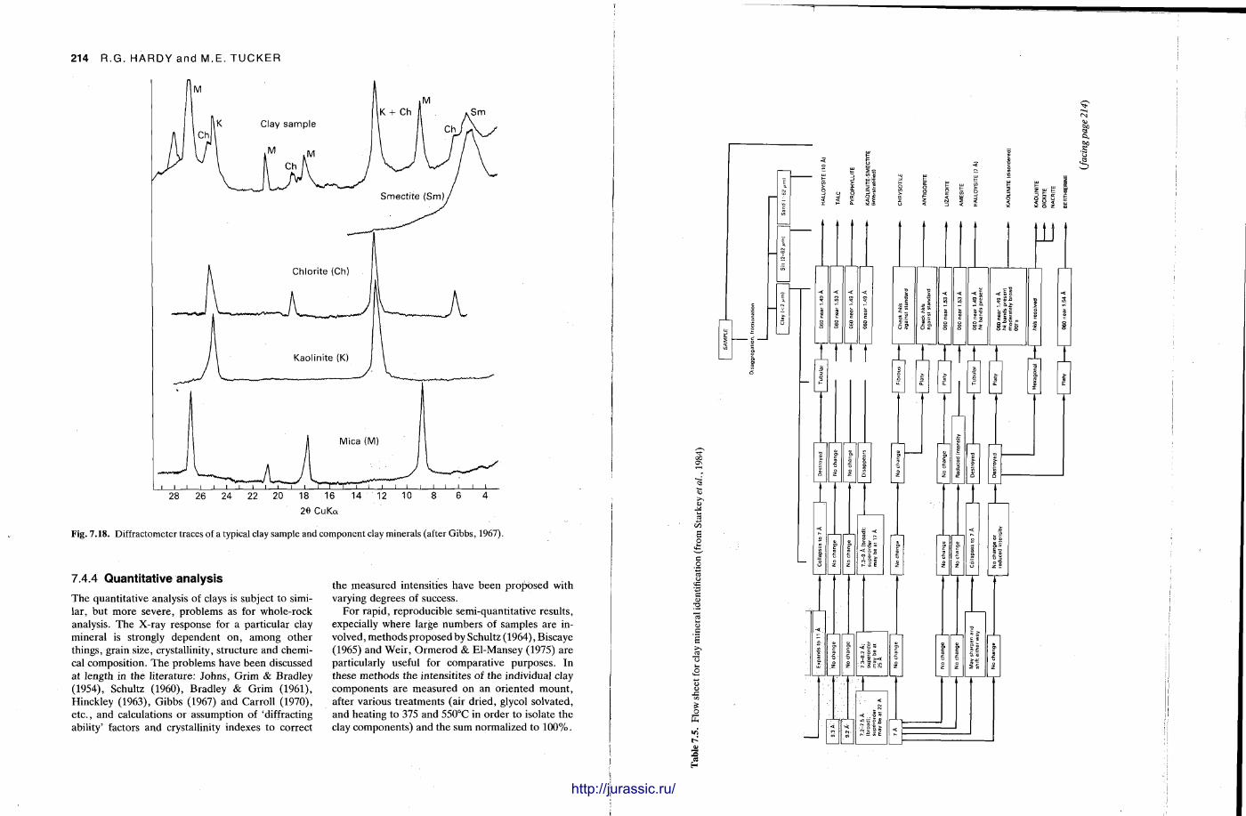
214 R.G. HARDY a n d M.E. TUCKER
2 6 C u K a
Fig. 7.18. Diffractometer traces of a typical clay sample and component clay minerals (after Gibbs, 1967).
7.4.4 Quantitative analysis
T h e quanti tat ive analysis of clays is subject to similar, but more severe, problems as for whole-rock analysis. The X-ray response for a particular clay mineral is strongly dependent on , among other things, grain size, crystallinity, s tructure and chemical composit ion. The problems have been discussed at length in the l i terature: Johns , Gr im & Bradley (1954), Schultz (1960), Bradley & Grim (1961), Hinckley (1963), Gibbs (1967) and Carroll (1970), e tc . , and calculations or assumption of 'diffracting ability' factors and crystallinity indexes to correct
the measured intensities have been proposed with varying degrees of success.
For rapid, reproducible semi-quantitative results, expecially where large numbers of samples are involved, methods proposed by Schultz (1964), Biscaye (1965) and Weir , Ormerod & El-Mansey (1975) are particularly useful for comparat ive purposes . In these methods the intensitites of the individual clay components are measured on an or iented moun t , after various t rea tments (air dr ied, glycol solvated, and heating to 375 and 550°C in order to isolate the clay components) and the sum normalized to 100%.
< y K Q
LLI
•a.
< < < I « l l < pu nd;
in 2 £ •D
Che
ck h
kls
agai
nst
sta
Che
ck h
kls
agai
nst s
ta
[ 06
0 ne
ar 1
.
060
near
1.
060
near
1.
hk b
ands
p
060
near
1.'
hk
ban
ds p
i m
oder
atel
y 00
1's
-C 060
near
1.
tttt rrTTr^s v
http://jurassic.ru/
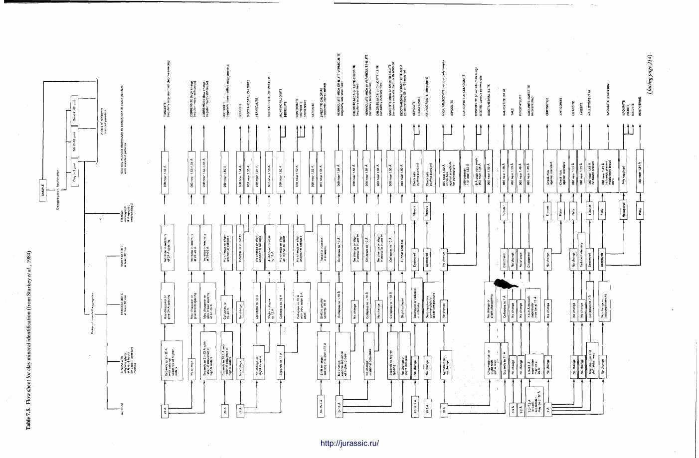
"5
E o is
u< <u c E >,
J3
a 4> to J3 cfl
CU
2'5
£ £ O 2 £ £ S- °
o 3 O £
5 d 8 S is < O D Up y S " 5 o 9 S _1 ID tc CO
If I f E
<—s
ft.
3 <
•g 3
~ uj i= £ UJ 01
i l l 1 2 0 Z CD
u < < s
i t i §
u U •o
o S1
< I s
" a l l j i l t
LI
I
or sligh
t inte
nsity
or slig
ht inte
nsity
o 10 A
|-
Ii! iii i 1
i i I
T T T T T T T T T T T T T T T T T T XX M f T X T T l
I XT
< I
11 < B> O
S "c 2
I
http://jurassic.ru/

2i X-RAY POWDER DIFFRACTION 215
Table 7.6. X-ray identification of the principal clay minerals (<2 um) in an oriented mount of a separated clay fraction from sedimentary material (from Carroll, 1970)
Mineral Basal d spacings (00/) Glycolation effect;
1 hr, 60°C Heating effect,
1 hr
Kaolinite
Kaolinite, disordered
Halloysite, 4 H 2 0 Halloysite, 2 H 2 0
Mica, 2M
Mite, lMd
Montmorillonite Group
Vermiculite
Chlorite, Mg-form
Chlorite, Fe-form
Mixed-layer minerals
Attapulgite (palygorskite)
Sepiolite
Amorphous clay, allophane
7.15 A (001); 3.75 A (002)
7.15 A (001) broad; 3.75 A broad
10 A (001) broad 7.2 A (001) broad
10 A (002); 5 A (004) generally referred to as (001) and (002)
10 A (002), broad, other basal spacings present but small
15 A (001) and integral series of basal spacings
14 A (001) and integral series of basal spacings
14 A (001) and integral series of basal spacings
14 A (001) less intense than in Mg-form; integral series of basal spacings
Regular, one (001) and integral series of basal spacings
Random, (001) is addition of individual minerals and depends on amount of those present
High intensity d reflections at 10,5,4.5,3.28,2.62 A
High intensity reflections at 12.6, 4.31,2.61 A
No d reflections
No change
No change
No change No change
No change
No change
(001) expands to 17 A with rational sequence of higher orders
No change
No change
No change
No change unless an expandable component is present
Expands if montmorillonite is a
constituent
No change
No change
No change
Becomes amorphous at 550-600°C
Becomes amorphous at lower temperatures than kaolinite
Dehydrates to 2H z O at 110°C Dehydrates at 125-150°C;
becomes amorphous at 560-590°C
(001) becomes more intense on heating but structure is maintained to 700°C
(001) noticeably more intense on heating as water layers are removed; at higher temperatures like mica
At 300°C (001) becomes 9 A
Dehydrates in steps
(001) increases in intensity; <800°C shows weight loss but no structural change
(001) scarcely increases; structure collapses below 800°C
Various, see descriptions of individual minerals
Depends on minerals present in inter-layered mineral
Dehydrates stepwise
Dehydrates and loses weight
http://jurassic.ru/
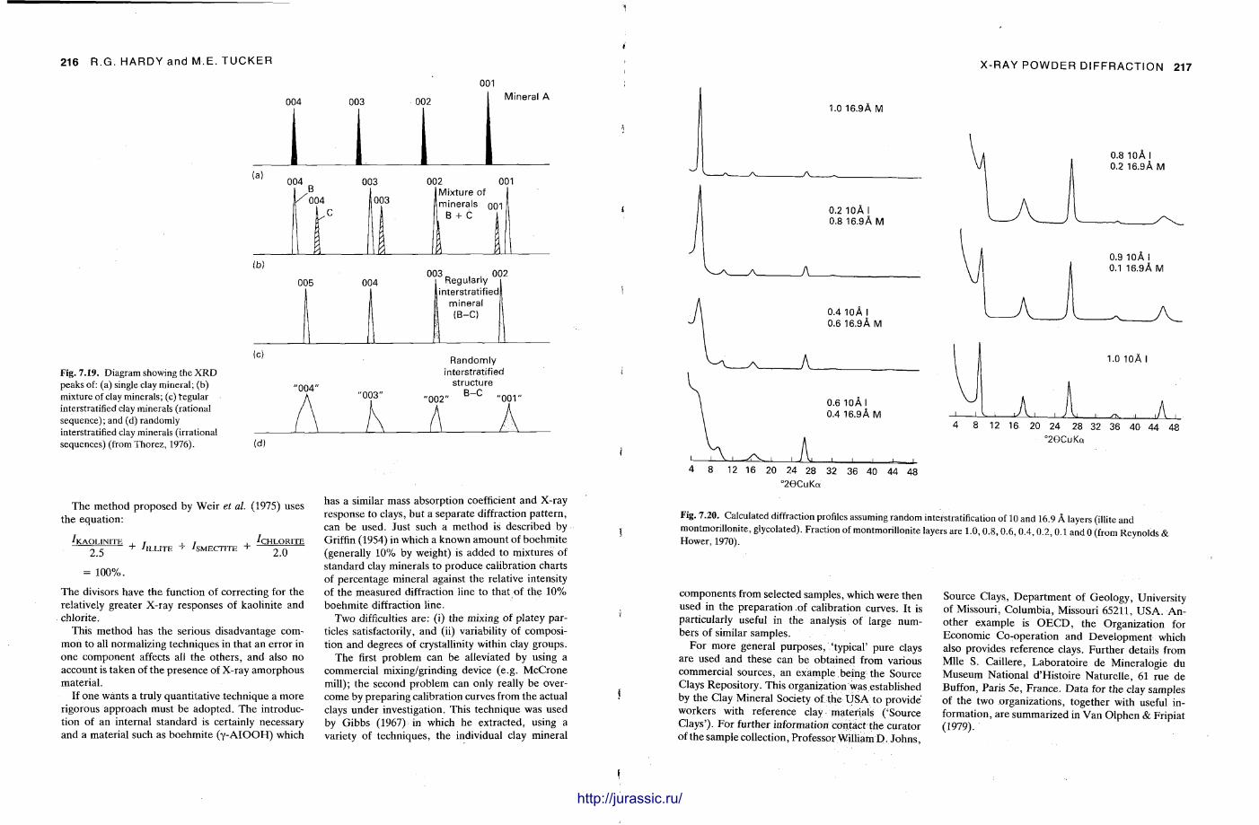
216 R.G. HARDY and M.E. TUCKER
001
004 003 002 Mineral A
(a) 004
I/004 003 002
(Mixture of ' I m i n e r a l s Q01
B + C
001
(b)
005 004 003 „ , , 002
Regularly |interstratified(
mineral (B-C)
(c)
Fig. 7.19. Diagram showing the XRD peaks of: (a) single clay mineral; (b) mixture of clay minerals; (c) tegular interstratified clay minerals (rational sequence); and (d) randomly interstratified clay minerals (irrational sequences) (fromThorez, 1976).
"004" "003" "002
Randomly interstratified
structure B-C 001"
(d)
The method proposed by Weir et al. (1975) uses the equat ion:
^ K A O L I N I T E . , . , , ^ C H L O R I T E 25 •'iLLiTE 1 • ' sMEcrrTE ' 20
= 100%.
The divisors have the function of correcting for the relatively greater X-ray responses of kaolinite and chlorite.
This method has the serious disadvantage common to all normalizing techniques in that an error in one component affects all the others , and also no account is taken of the presence of X-ray amorphous material .
If one wants a truly quanti tat ive technique a more rigorous approach must be adopted . T h e introduction of an internal s tandard is certainly necessary and a material such as boehmite ( y - A I O O H ) which
has a similar mass absorption coefficient and X-ray response to clays, but a separate diffraction pat tern, can be used. Just such a method is described by Griffin (1954) in which a known amount of boehmite (generally 10% by weight) is added to mixtures of standard clay minerals to produce calibration charts of percentage mineral against the relative intensity of the measured diffraction line to that of the 10% boehmite diffraction line.
Two difficulties a re : (i) the mixing of platey particles satisfactorily, and (ii) variability of composition and degrees of crystallinity within clay groups.
T h e first problem can be alleviated by using a commercial mixing/grinding device (e.g. McCrone mill); the second problem can only really be overcome by preparing calibration curves from the actual clays under investigation. This technique was used by Gibbs (1967) in which he extracted, using a variety of techniques, the individual clay mineral
X-RAY POWDER DIFFRACTION 217
1.0 16.9A M
°2eCuKa
Fig. 7.20. Calculated diffraction profiles assuming random interstratification of 10 and 16.9 A layers (illite and montmorillonite, glycolated). Fraction of montmorillonite layers are 1.0,0.8,0.6,0.4,0.2 0 1 and 0 (from Reynolds & Hower, 1970).
components from selected samples , which were then used in the preparat ion of calibration curves. It is particularly useful in the analysis of large numbers of similar samples.
For more general purposes , ' typical ' pure clays are used and these can be obtained from various commercial sources, an example being the Source Clays Repository. This organization was established by the Clay Mineral Society of the U S A to provide workers with reference clay materials ( 'Source Clays') . For further information contact the curator of t he sample collection, Professor William D . Johns ,
Source Clays, Depa r tmen t of Geology, University of Missouri , Columbia , Missouri 65211, USA.. Another example is O E C D , the Organization for Economic Co-operat ion and Development which also provides reference clays. Fur ther details from Mile S. Caillere, Labora to i re d e Mineralogie du Museum National d 'Histoire Naturel le , 61 rue de Buffon, Paris 5e, France . D a t a for the clay samples of the two organizations, together with useful information, are summarized in V a n Olphen & Fripiat (1979).
http://jurassic.ru/
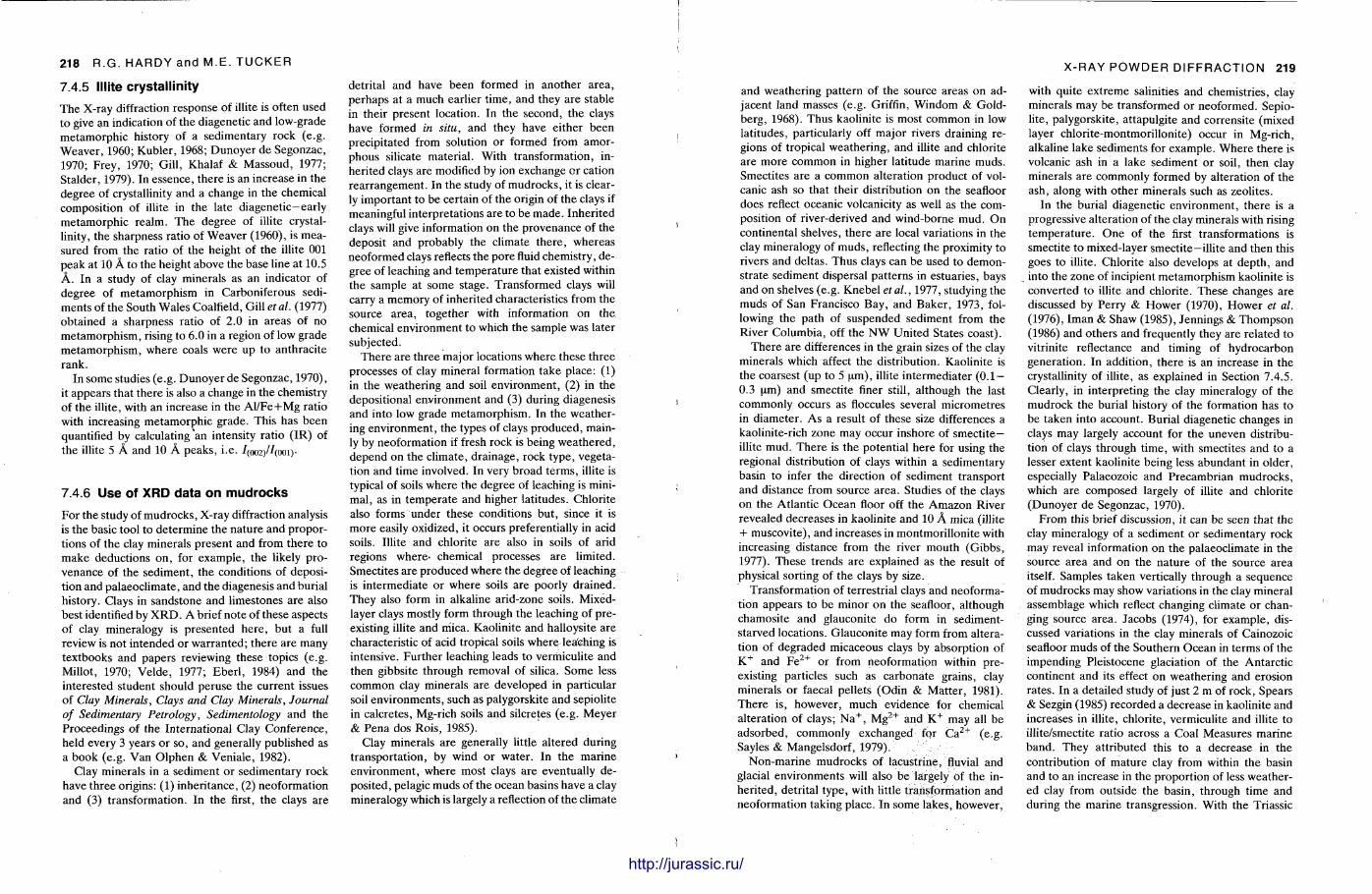
218 R.G. HARDY and M.E. TUCKER
7.4.5 Mite crystal l inity
The X-ray diffraction response of illite is often used to give an indication of the diagenetic and low-grade metamorphic history of a sedimentary rock (e.g. Weaver , 1960; Kubler , 1968; Dunoyer de Segonzac, 1970; Frey, 1970; Gill, Khalaf & Massoud, 1977; Stalder, 1979). In essence, there is an increase in the degree of crystallinity and a change in the chemical composit ion of illite in the late d iagene t i c -ea r ly metamorphic realm. The degree of illite crystallinity, the sharpness ratio of Weaver (1960), is measured from the ratio of the height of the illite 001 peak at 10 A to the height above the base line at 10.5 A . In a study of clay minerals as an indicator of degree of metamorphism in Carboniferous sediments of the South Wales Coalfield, Gill et al. (1977) obtained a sharpness ratio of 2.0 in areas of no metamorphism, rising to 6.0 in a region of low grade metamorphism, where coals were up to anthracite rank.
In some studies (e.g. Dunoyer de Segonzac, 1970), it appears that there is also a change in the chemistry of the illite, with an increase in the A l / F e + M g ratio with increasing metamorphic grade. This has been quantified by calculating "an intensity ratio ( IR) of the illite 5 A and 10 A peaks , i.e. 7(oo2)/7(ooi)-
7.4.6 Use of XRD data on mudrocks
For the study of mudrocks , X-ray diffraction analysis is the basic tool to determine the nature and proportions of the clay minerals present and from there to make deductions on , for example , the likely provenance of the sediment , the conditions of deposition and palaeocl imate, and the diagenesis and burial history. Clays in sandstone and limestones are also best identified by X R D . A brief note of these aspects of clay mineralogy is presented he re , but a full review is not in tended or warranted; there are many textbooks and papers reviewing these topics (e.g. Millot, 1970; Velde , 1977; Eber l , 1984) and the interested student should peruse the current issues of Clay Minerals, Clays and Clay Minerals, Journal of Sedimentary Petrology, Sedimentology and the Proceedings of the International Clay Conference, held every 3 years or so, and generally published as a book (e.g. Van Olphen & Veniale , 1982).
Clay minerals in a sediment or sedimentary rock have three origins: (1) inheri tance, (2) neoformation and (3) transformation. In the first, the clays are
detrital and have been formed in another area , perhaps at a much earlier t ime, and they are stable in their present location. In the second, the clays have formed in situ, and they have either been precipitated from solution or formed from amorphous silicate material . With transformation, inherited clays are modified by ion exchange or cation rear rangement . In the study of mudrocks , it is clearly important to be certain of the origin of the clays if meaningful interpretat ions are to be made . Inheri ted clays will give information on the provenance of the deposit and probably the climate there , whereas neoformed clays reflects the pore fluid chemistry, degree of leaching and tempera ture that existed within the sample at some stage. Transformed clays will carry a memory of inherited characteristics from the source area , together with information on the chemical environment to which the sample was later subjected.
There are three major locations where these three processes of clay mineral formation take place: (1) in the weathering and soil environment , (2) in the depositional environment and (3) during diagenesis and into low grade metamorphism. In the weathering environment , the types of clays produced, mainly by neoformation if fresh rock is being weathered , depend on the climate, drainage, rock type, vegetation and t ime involved. In very broad t e rms , illite is typical of soils where the degree of leaching is minimal , as in t empera te and higher lati tudes. Chlori te also forms under these conditions but , since it is more easily oxidized, it occurs preferentially in acid soils. Illite and chlorite are also in soils of arid regions where- chemical processes are limited. Smectites are produced where the degree of leaching is intermediate or where soils are poorly drained. They also form in alkaline arid-zone soils. Mixed-layer clays mostly form through the leaching of preexisting illite and mica. Kaolinite and halloysite are characteristic of acid tropical soils where leaching is intensive. Fur ther leaching leads to vermiculite and then gibbsite through removal of silica. Some less common clay minerals are developed in particular soil environments , such as palygorskite and sepiolite in calcretes, Mg-rich soils and silcretes (e .g. Meyer & Pena dos Rois , 1985).
Clay minerals are generally little al tered during t ransporta t ion, by wind or water . In the marine environment , where most clays are eventually deposited, pelagic muds of the ocean basins have a clay mineralogy which is largely a reflection of the climate
X-RAY POWDER DIFFRACTION 219
and weathering pat tern of the source areas on adjacent land masses (e.g. Griffin, Windom & Goldberg, 1968). Thus kaolinite is most common in low latitudes, particularly off major rivers draining regions of tropical weathering, and illite and chlorite are more common in higher latitude marine muds. Smectites are a common alteration product of volcanic ash so that their distribution on the seafloor does reflect oceanic volcanicity as well as the composition of river-derived and wind-borne mud. O n continental shelves, there are local variations in the clay mineralogy of muds , reflecting the proximity to rivers and deltas. Thus clays can be used to demonstrate sediment dispersal pat terns in estuaries, bays and on shelves (e.g. Knebel et al., 1977, studying the muds of San Francisco Bay, and Baker , 1973, following the path of suspended sediment from the River Columbia, off the N W United States coast) .
There are differences in the grain sizes of the clay minerals which affect the distribution. Kaolinite is the coarsest (up to 5 um) , illite intermediater (0.1 — 0.3 um) and smectite finer still, al though the last commonly occurs as floccules several micrometres in diameter . As a result of these size differences a kaolinite-rich zone may occur inshore of smectite— illite mud. There is the potential here for using the regional distribution of clays within a sedimentary basin to infer the direction of sediment t ransport and distance from source area . Studies of the clays on the Atlant ic Ocean floor off the Amazon River revealed decreases in kaolinite and 10 A mica (illite + muscovite), and increases in montmoril lonite with increasing distance from the river mouth (Gibbs , 1977). These t rends are explained as the result of physical sorting of the clays by size.
Transformation of terrestrial clays and neoformation appears to be minor on the seafloor, although chamosite and glauconite do form in sediment-starved locations. Glauconite may form from alteration of degraded micaceous clays by absorption of K + and F e 2 + or from neoformation within preexisting particles such as carbonate grains, clay minerals or faecal pellets (Odin & Mat ter , 1981). The re is, however , much evidence for chemical alteration of clays; N a + , M g 2 + and K + may all be adsorbed, commonly exchanged for C a 2 + (e.g. Sayles & Mangelsdorf, 1979).
Non-marine mudrocks of lacustrine, fluvial and glacial environments will also be largely of the inheri ted, detrital type, with little transformation and neoformation taking place. In some lakes, however,
with quite ext reme salinities and chemistries, clay minerals may be transformed or neoformed. Sepiolite, palygorskite, attapulgite and corrensite (mixed layer chlorite-montmoril lonite) occur in Mg-rich, alkaline lake sediments for example . Where there is volcanic ash in a lake sediment or soil, then clay minerals are commonly formed by alteration of the ash, along with other minerals such as zeolites.
In the burial diagenetic environment , there is a progressive alteration of the clay minerals with rising tempera ture . O n e of the first transformations is smectite to mixed-layer smectite—illite and then this goes to illite. Chlori te also develops at depth , and into the zone of incipient metamorphism kaolinite is converted to illite and chlorite. These changes are discussed by Perry & Hower (1970), Hower et al. (1976), Iman & Shaw (1985), Jennings & Thompson (1986) and others and frequently they are related to vitrinite reflectance and timing of hydrocarbon generat ion. In addi t ion, there is an increase in the crystallinity of illite, as explained in Section 7.4.5. Clearly, in interpreting the clay mineralogy of the mudrock the burial history of the formation has to be taken into account. Burial diagenetic changes in clays may largely account for the uneven distribution of clays through t ime, with smectites and to a lesser extent kaolinite being less abundant in older, especially Palaeozoic and Precambrian mudrocks , which are composed largely of illite and chlorite (Dunoyer de Segonzac, 1970).
F rom this brief discussion, it can be seen that the clay mineralogy of a sediment or sedimentary rock may reveal information on the palaeoclimate in the source area and on the na ture of the source area itself. Samples taken vertically through a sequence of mudrocks may show variations in the clay mineral assemblage which reflect changing climate or changing source area. Jacobs (1974), for example, discussed variations in the clay minerals of Cainozoic seafloor muds of the Southern Ocean in terms of the impending Pleistocene glaciation of the Antarct ic continent and its effect on weathering and erosion rates. In a detailed study of just 2 m of rock, Spears & Sezgin (1985) recorded a decrease in kaolinite and increases in illite, chlorite, vermiculite and illite to illite/smectite ratio across a Coal Measures marine band. They at tr ibuted this to a decrease in the contribution of mature clay from within the basin and to an increase in the proport ion of less weathered clay from outside the basin, through time and during the marine transgression. With the Triassic
iitmwmiittiiiiiiimiiiiiini http://jurassic.ru/
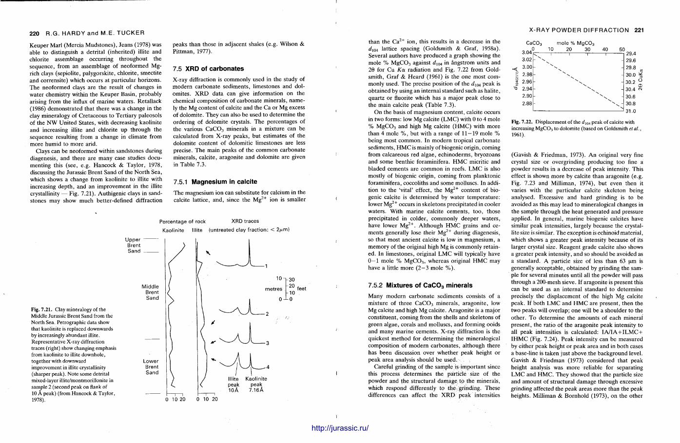
220 R . G . H A R D Y a n d M . E . T U C K E R
Keuper Marl (Mercia Mudstones) , Jeans (1978) was able to distinguish a detrital ( inheri ted) illite and chlorite assemblage occurring throughout the sequence, from an assemblage of neoformed Mg-rich clays (sepiolite, palygorskite, chlorite, smectite and corrensite) which occurs at particular horizons. T h e neoformed clays a r e the result of changes in water chemistry within the Keuper Basin, probably arising from the influx of marine waters . Retallack (1986) demonstra ted that there was a change in the clay mineralogy of Cretaceous to Tert iary paleosols of the N W United States, with decreasing kaolinite and increasing illite and chlorite up through the sequence resulting from a change in climate from more humid to more arid.
Clays can be neoformed within sandstones during diagenesis, and there a re many case studies documenting this (see, e.g. Hancock & Taylor , 1978, discussing the Jurassic Brent Sand of the Nor th Sea, which shows a change from kaolinite to illite with increasing depth , and an improvement in the illite crystallinity — Fig. 7.21). Authigenic clays in sandstones may show much better-defined diffraction
peaks than those in adjacent shales (e.g. Wilson & Pi t tman, 1977).
7.5 XRD of carbonates
X-ray diffraction is commonly used in the study of modern carbonate sediments , l imestones and dolomites . X R D data can give information on the chemical composit ion of carbonate minerals, namely the Mg content of calcite and the Ca or Mg excess of dolomite . They can also be used to determine the ordering of dolomite crystals. T h e percentages of the various C a C 0 3 minerals in a mixture can be calculated from X-ray peaks , but estimates of the dolomite content of dolomitic l imestones are less precise. The main peaks of the common carbonate minerals , calcite, aragonite and dolomite a re given in Table 7.3.
7.5.1 Magnesium in calcite
T h e magnesium ion can substi tute for calcium in the calcite lattice, and, since the Mg2"1" ion is smaller
Fig. 7.21. Clay mineralogy of the Middle Jurassic Brent Sand from the North Sea. Petrographic data show that kaolinite is replaced downwards by increasingly abundant illite. Representative X-ray diffraction traces (right) show changing emphasis from kaolinite to illite downhole, together with downward improvement in illite crystallinity (sharper peak). Note some detrital mixed-layer illite/montmorillonite in sample 2 (second peak on flank of 10 A peak) (from Hancock & Taylor, 1978).
Percentage of rock XRD traces Kaolinite Illite (untreated clay fraction: < 2/u,m)
Upper Brent Sand
Middle Brent Sand
Lower Brent Sand
feet
Kaolinite peak
7.16A
0 10 20 10 20
I MlllllllllltlllttMllllllllf
X - R A Y P O W D E R D I F F R A C T I O N 221
than the C a 2 + ion, this results in a decrease in the rf104 lattice spacing (Goldsmith & Graf, 1958a). Several authors have produced a graph showing the mole % M g C 0 3 against d m in angstrom units and 20 for Cu Ka radiation and Fig. 7.22 from Goldsmith, Graf & Heard (1961) is the one most commonly used. The precise position of the rf104 peak is obtained by using an internal s tandard such as halite, quar tz or fluorite which has a major peak close to the main calcite peak (Table 7.3).
On the basis of magnesium content , calcite occurs in two forms: low Mg calcite (LMC) with 0 to 4 mole % M g C 0 3 and high Mg calcite ( H M C ) with more than 4 mole % , but with a range of 1 1 - 1 9 mole % being most common. In modern tropical carbonate sediments , H M C is mainly of biogenic origin, coming from calcareous red algae, echinoderms, bryozoans and some benthic foraminifera. H M C micritic and bladed cements are common in reefs. L M C is also mostly of biogenic origin, coming from planktonic foraminifera, coccoliths and some molluscs. In addition to the 'vital ' effect, the M g 2 + content of biogenic calcite is determined by water t empera ture : lower M g 2 + occurs in skeletons precipitated in cooler waters . With marine calcite cements , too , those precipitated in colder, commonly deeper waters , have lower M g 2 + . Al though H M C grains and cements generally lose their M g 2 + during diagenesis, so that most ancient calcite is low in magnesium, a memory of the original high Mg is commonly retained. In l imestones, original L M C will typically have 0—1 mole % M g C 0 3 , whereas original H M C may have a little more (2—3 mole % ) .
7.5.2 Mixtures of C a C 0 3 minerals
Many modern carbonate sediments consists of a mixture of three C a C 0 3 minerals , aragonite , low Mg calcite and high Mg calcite. Aragoni te is a major consti tuent, coming from the shells and skeletons of green algae, corals and molluscs, and forming ooids and many marine cements . X-ray diffraction is the quickest method for determining the mineralogical composit ion of modern carbonates , although there has been discussion over whether peak height or peak area analysis should be used.
Careful grinding of the sample is important since this process determines the particle size of the powder and the structural damage to the minerals, which respond differently to the grinding. These differences can affect the X R D peak intensities
CaC0 3 mole % MgC0 3
.0 10 20 30 3.04 3.02 3.00 2.98 2.96 2.94 2.90 2.88
40 50 I I I I
-\
\
\ \
\ \
\ \
- \ \
\
N
29.4 29.6 29.8 s
30.0 * 30.2 °
CD 30.4 «m
30.6 30.8 31.0
Fig. 7.22. Displacement of the di(H peak of calcite with increasing M g C 0 3 to dolomite (based on Goldsmith et al. 1961).
(Gavish & Fr iedman, 1973). A n original very fine crystal size or overgrinding producing too fine a powder results in a decrease of peak intensity. This effect is shown more by calcite than aragonite (e.g. Fig. 7.23 and Milliman, 1974), but even then it varies with the particular calcite skeleton being analysed. Excessive and hard grinding is to be avoided as this may lead to mineralogical changes in the sample through the heat generated and pressure applied. In general , marine biogenic calcites have similar peak intensities, largely because the crystallite size is similar. The exception is echinoid material , which shows a greater peak intensity because of its larger crystal size. Reagen t grade calcite also shows a greater peak intensity, and so should be avoided as a s tandard. A particle size of less than 63 um is generally acceptable, obtained by grinding the sample for several minutes until all the powder will pass through a 200-mesh sieve. If aragonite is present this can be used as an internal s tandard to determine precisely the displacement of the high Mg calcite peak. If both L M C and H M C are present , then the two peaks will overlap; one will be a shoulder to the other . T o determine the amounts of each mineral present , the ratio of the aragonite peak intensity to all peak intensities is calculated: I A / I A + I L M C + I H M C (Fig. 7.24). Peak intensity can be measured by either peak height or peak area and in both cases a base-line is taken just above the background level. Gavish & Friedman (1973) considered that peak height analysis was more reliable for separating L M C and H M C . They showed that the particle size and amount of structural damage through excessive grinding affected the peak areas more than the peak heights. Milliman & Bornhold (1973), on the other
http://jurassic.ru/
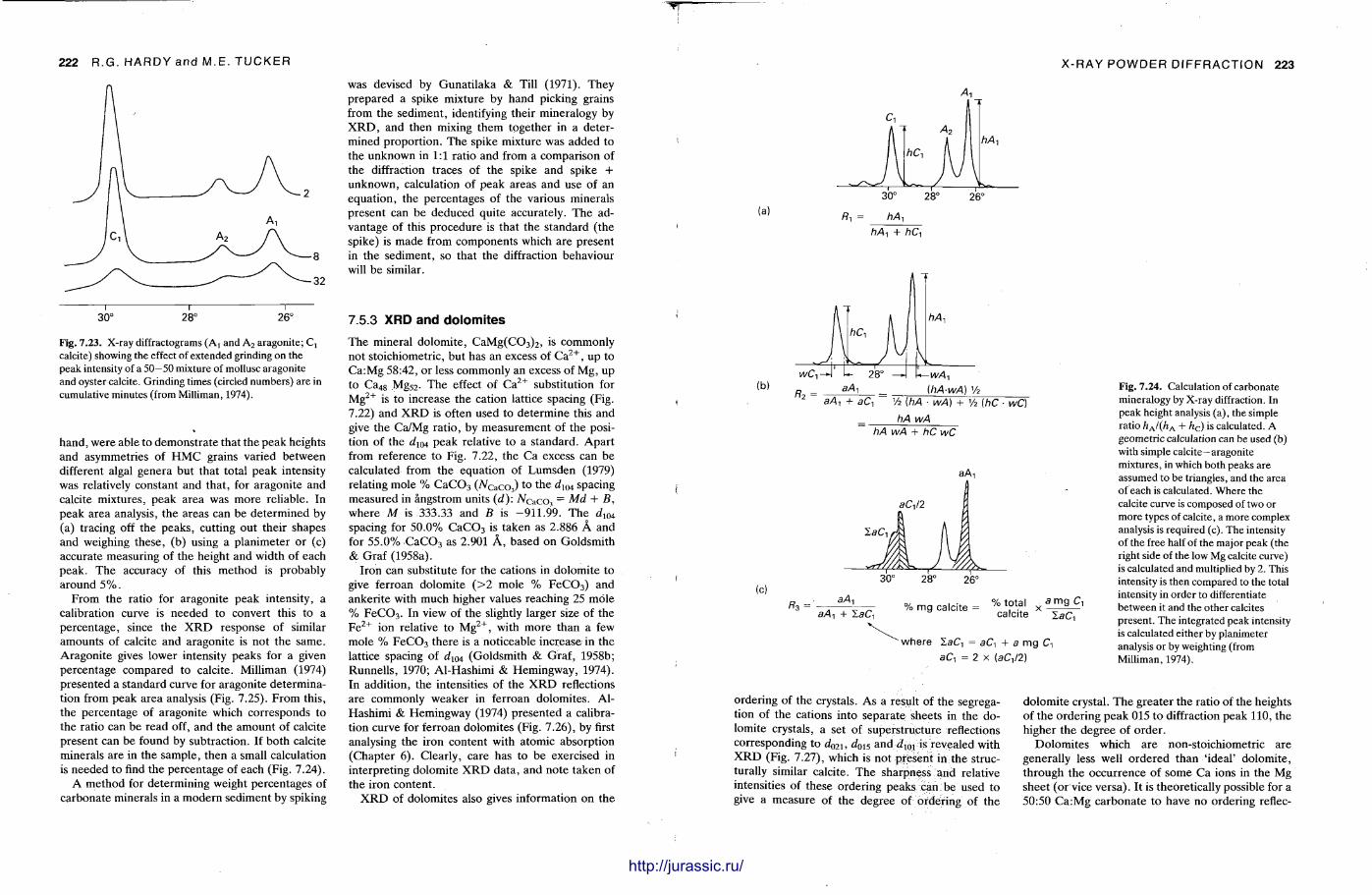
2 2 2 R.G. HARDY and M.E. TUCKER
i 1 r~ 30° 28° 26° Fig. 7.23. X-ray diffractograms (A, and A 2 aragonite; C,
calcite) showing the effect of extended grinding on the peak intensity of a 50—50 mixture of mollusc aragonite and oyster calcite. Grinding times (circled numbers) are in cumulative minutes (from Milliman, 1974).
hand , were able to demonst ra te that the peak heights and asymmetries of H M C grains varied between different algal genera but that total peak intensity was relatively constant and that , for aragonite and calcite mixtures, peak area was more reliable. In peak area analysis, the areas can be de termined by (a) tracing off the peaks , cutting out their shapes and weighing these , (b) using a planimeter or (c) accurate measuring of the height and width of each peak. The accuracy of this method is probably around 5 % .
F rom the ratio for aragonite peak intensity, a calibration curve is needed to convert this to a percentage, since the X R D response of similar amounts of calcite and aragonite is not the same. Aragoni te gives lower intensity peaks for a given percentage compared to calcite. Milliman (1974) presented a s tandard curve for aragonite determination from peak area analysis (Fig. 7.25). F rom this, the percentage of aragonite which corresponds to the ratio can be read off, and the amount of calcite present can be found by subtraction. If both calcite minerals are in the sample , then a small calculation is needed to find the percentage of each (Fig. 7.24).
A method for determining weight percentages of carbonate minerals in a modern sediment by spiking
was devised by Gunat i laka & Till (1971). They prepared a spike mixture by hand picking grains from the sediment , identifying their mineralogy by X R D , and then mixing them together in a determined propor t ion. The spike mixture was added to the unknown in 1:1 ratio and from a comparison of the diffraction traces of the spike and spike + unknown, calculation of peak areas and use of an equat ion, the percentages of the various minerals present can be deduced quite accurately. The advantage of this procedure is that the s tandard (the spike) is made from components which are present in the sediment , so that the diffraction behaviour will be similar.
7.5.3 XRD and dolomites
The mineral dolomite , C a M g ( C 0 3 ) 2 , is commonly not stoichiometric, but has an excess of C a 2 + , up to Ca :Mg 58:42, or less commonly an excess of Mg, up to C a 4 8 Mg52- The effect of C a 2 + substitution for M g 2 + is to increase the cation lattice spacing (Fig. 7.22) and X R D is often used to determine this and give the Ca/Mg rat io , by measurement of the position of the dW4 peak relative to a s tandard. Apar t from reference to Fig. 7.22, the Ca excess can be calculated from the equat ion of Lumsden (1979) relating mole % C a C 0 3 (AfCaCo3) to the dW4 spacing measured in angstrom units (d): AfCaCo, = Md + B, where M is 333.33 and B is - 9 1 1 . 9 9 . T h e dlM
spacing for 50 .0% C a C 0 3 is taken as 2.886 A and for 55 .0% C a C 0 3 as 2.901 A , based on Goldsmith & Graf (1958a).
Iron can substitute for the cations in dolomite to give ferroan dolomite ( > 2 mole % F e C 0 3 ) and ankeri te with much higher values reaching 25 mole % F e C 0 3 . In view of the slightly larger size of the F e 2 + ion relative to M g 2 + , with more than a few mole % F e C 0 3 there is a noticeable increase- in the lattice spacing of dW4 (Goldsmith & Graf, 1958b; Runnel ls , 1970; Al-Hashimi & Hemingway, 1974). In addit ion, the intensities of the X R D reflections are commonly weaker in ferroan dolomites. Al-Hashimi & Hemingway (1974) presented a calibration curve for ferroan dolomites (Fig. 7.26), by first analysing the iron content with atomic absorption (Chapter 6) . Clearly, care has to be exercised in interpreting dolomite X R D data , and note taken of the iron content .
X R D of dolomites also gives information on the
X-RAY POWDER DIFFRACTION 2 2 3
hA-, hA-, + hC-,
(b) U— wAi
(hA-wA) V2
aA-, + aCi V* {hA • wA) + V2 (hC • wC) _ hA wA
hA wA + hC wC
(c) aA-,
aA-, + S a d % m g calcite = % t { * ? ' x * m g C l
calcite SaCi
~ where laC-, = aC-, + a mg aC, = 2 x (ad /2)
Fig. 7.24. Calculation of carbonate mineralogy by X-ray diffraction. In peak height analysis (a), the simple ratio hA/(hA + hc) is calculated. A geometric calculation can be used (b) with simple calcite—aragonite mixtures, in which both peaks are assumed to be triangles, and the area of each is calculated. Where the calcite curve is composed of two or more types of calcite, a more complex analysis is required (c). The intensity of the free half of the major peak (the right side of the low Mg calcite curve) is calculated and multiplied by 2. This intensity is then compared to the total intensity in order to differentiate between it and the other calcites present. The integrated peak intensity is calculated either by planimeter analysis or by weighting (from Milliman, 1974).
order ing of the crystals. As a result of the segregation of the cations into separate sheets in the dolomite crystals, a set of superstructure reflections corresponding to d 02i> ^ois and d n n is revealed with X R D (Fig. 7.27), which is not present in the structurally similar calcite. The sharpness and relative intensities of these ordering peaks can be used to give a measure of the degree of ordering of the
dolomite crystal. T h e greater the ratio of the heights of the order ing peak 015 to diffraction peak 110, the higher the degree of order .
Dolomi tes which are non-stoichiometric are generally less well o rde red than ' ideal ' dolomite , th rough the occurrence of some Ca ions in the Mg sheet (or vice versa) . It is theoretically possible for a 50:50 C a : M g carbonate to have no ordering reflec-
http://jurassic.ru/
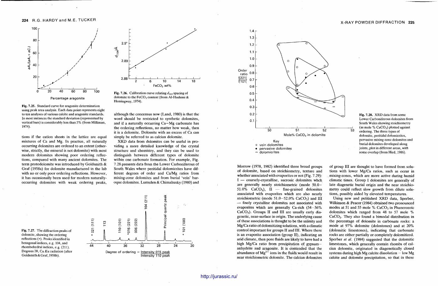
224 R.G. HARDY and M.E. TUCKER
100
80
60
to 40
20 A '
0 20 40 60 80 100
Percentage aragonite
Fig. 7.25. Standard curve for aragonite determination using peak area analysis. Each data point represents eight to ten analyses of various calcite and aragonite standards. In most instances the standard deviation (represented by vertical bars) is considerably less than 5% (from Milliman, 1974).
tions if the cation sheets in the lattice are equal mixtures of Ca and Mg. In practice, all naturally occurring dolomites are ordered to an extent (otherwise, strictly, the mineral is not dolomite) with most modern dolomites showing poor order ing reflections, compared with many ancient dolomites . The term protodolomite was introduced by Goldsmith & Graf (1958a) for dolomite manufactured in the lab with no or only poor ordering reflections. However , it has occasionally been used for modern naturally-occurring dolomites with weak order ing peaks ,
<
o
2.9°
2.89
2.88 6 10 14 18
FeC0 3 wt%
Fig. 7.26. Calibration curve relating d104 spacing of dolomite to the F e C 0 3 content (from Al-Hashimi & Hemingway, 1974).
al though the concensus now (Land, 1980) is that the word should be restricted to synthetic dolomites , and if a naturally occurring Ca—Mg carbonate has the order ing reflections, no mat ter how weak, then it is a dolomite . Dolomite with an excess of Ca can simply be referred to as calcian dolomite .
X R D data from dolomites can be useful in providing a more detailed knowledge of the crystal structure and chemistry, and they can be used to distinguish between different types of dolomite within one carbonate formation. For example , Fig. 7.28 presents data from the Lower Carboniferous of South Wales where peritidal dolomicrites have different degrees of order and Ca/Mg ratios from mixing-zone dolomites and from burial 'vein' baroque dolomites. Lumsden & Chimahusky (1980) and
Fig. 7.27. The diffraction peaks of dolomite, showing the ordering reflections (*). Peaks identified in hexagonal indices, e.g. 104, and rhombohedral indices, e.g. (211). Degrees 29, Cu Koc radiation (after Goldsmith & Graf, 1958b).
Degree of ordering Intensity 015 peak Intensity 110 peak
.ll Mi l l
X-RAY POWDER DIFFRACTION 225
Order ratio
l[221] l[101]
1.4
1.3
1.2
1.1 h
1.0
0.9
0.8
0.7
0.6
0.5
0.4
0.3
0.2
0.1
50 51 52 Mole% C a C 0 3 in dolomite
Key vein dolomites pervasive dolomites dolomicrites
53
Fig. 7.28. XRD data from some Lower Carboniferous dolomites from South Wales showing stoichiometry (as mole % CaC0 3 ) plotted against ordering. The three types of dolomite, peritidal dolomicrites, pervasive mixing-zone dolomites and burial dolomites developed along joints, plot in different areas, with some overlap (from Hird, 1986).
Morrow (1978, 1982) identified three broad groups of dolomite , based on stoichiometry, texture and whether associated with evaporites or not (Fig. 7.29): I — coarsely-crystalline, sucrosic dolomites whch are generally nearly stoichiometric (mode 50.0— 51.0% C a C Q 3 ) , I I — fine-grained dolomites associated with evaporites which are also nearly stoichiometric (mode 5 1 . 0 - 5 2 . 0 % C a C 0 3 ) and III — finely crystalline dolomites not associated with evaporites which are generally Ca-rich ( 5 4 - 5 6 % C a C 0 3 ) . Groups II and III are usually early diagenetic, near-surface in origin. The underlying cause of these associations is thought to be the salinity and Mg/Ca ratio of dolomitizing solutions, with a climatic control important for groups II and III . Where there is an evapori te association (group I I ) , indicating an arid cl imate, then pore fluids are likely to have had a high Mg/Ca ratio from precipitation of gypsum— anhydrite and aragoni te . It is contended that the abundance of M g 2 + ions in the fluids would result in near stoichiometric dolomite . The calcian dolomites
of group III are thought to have formed from solutions with lower Mg/Ca ratios, such as occur in mixing-zones, which are more active during humid climatic t imes. G r o u p I dolomites are generally of late diagenetic burial origin and the near stoichiometry could reflect slow growth from dilute solutions, possibly aided by elevated tempera tures .
Using new and published X R D data , Sperber , Wilkinson & Peacor (1984) obtained two pronounced modes at 51 and 55 mole % C a C 0 3 in Phanerozoic dolomites which ranged from 48 to 57 mole % C a C 0 3 . They also found a bimodal distribution in the percentage of dolomite in carbonate rocks: a mode at 9 7 % dolomite (dolostones) and at 2 0 % (dolomitic l imestones), indicating that carbonate rocks are either partially or completely dolomitized. Sperber et al. (1984) suggested that the dolomitic l imestones, which generally contain rhombs of calcian dolomite , originated in diagenetically closed systems during high Mg calcite dissolution — low Mg calcite and dolomite precipitation, so that in these
http://jurassic.ru/
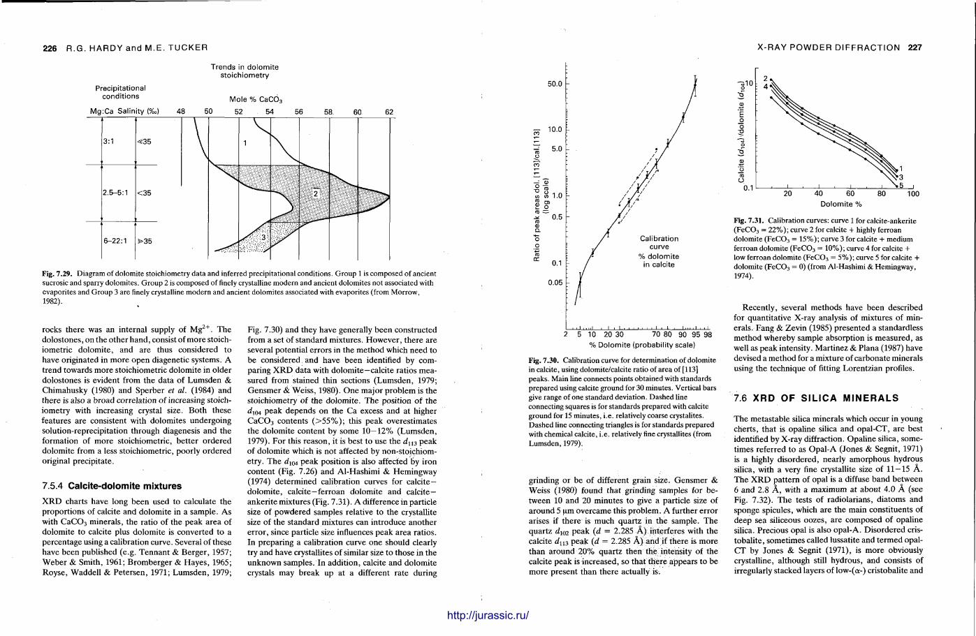
226 R.G. HARDY and M.E. TUCKER
Trends in dolomite stoichiometry
Precipitational conditions
Mg:Ca Salinity (%>) 48 50 Mole % CaC0 3
52 54
Fig. 7.29. Diagram of dolomite stoichiometry data and inferred precipitational conditions. Group 1 is composed of ancient sucrosic and sparry dolomites. Group 2 is composed of finely crystalline modern and ancient dolomites not associated with evaporites and Group 3 are finely crystalline modern and ancient dolomites associated with evaporites (from Morrow, 1982).
rocks there was an internal supply of Mg . T h e dolostones, on the other hand , consist of more stoichiometric dolomite , and are thus considered to have originated in more open diagenetic systems. A trend towards more stoichiometric dolomite in older dolostones is evident from the data of Lumsden & Chimahusky (1980) and Sperber et al. (1984) and there is also a broad correlation of increasing stoichiometry with increasing crystal size. Both these features are consistent with dolomites undergoing solution-reprecipitation through diagenesis and the formation of more stoichiometric, be t ter ordered dolomite from a less stoichiometric, poorly ordered original precipitate.
7.5.4 Calcite-dolomite mixtures
X R D charts have long been used to calculate the proport ions of calcite and dolomite in a sample . As with C a C 0 3 minerals , the ratio of the peak area of dolomite to calcite plus dolomite is converted to a percentage using a calibration curve. Several of these have been published (e.g. Tennan t & Berger , 1957; Weber & Smith, 1961; Bromberger & Hayes , 1965; Royse , Waddell & Petersen, 1971; Lumsden , 1979;
Fig. 7.30) and they have generally been constructed from a set of s tandard mixtures. However , there are several potential errors in the method which need to be considered and have been identified by comparing X R D data with dolomite—calcite ratios measured from stained thin sections (Lumsden , 1979; Gensmer & Weiss, 1980). One major p roblem is the stoichiometry of the dolomite . The position of the d 1 04 peak depends on the Ca excess and at higher C a C 0 3 contents ( > 5 5 % ) ; this peak overest imates the dolomite content by some 10—12% (Lumsden , 1979). For this reason, it is best to use the dU3 peak of dolomite which is not affected by non-stoichiom-etry. T h e dW4 peak position is also affected by iron content (Fig. 7.26) and Al-Hashimi & Hemingway (1974) determined calibration curves for c a l c i t e -dolomite , calcite—ferroan dolomite and calcite— ankeri te mixtures (Fig. 7.31). A difference in particle size of powdered samples relative to the crystallite size of the standard mixtures can introduce another error , since particle size influences peak area rat ios. In preparing a calibration curve one should clearly try and have crystallites of similar size to those in the unknown samples. In addit ion, calcite and dolomite crystals may break up at a different rate during
HHnmmTiiHmtM»iii»»tiMMif»m»Hffl
X-RAY POWDER DIFFRACTION 227
1 . . i . . . . i • i . i i . i . i 2 5 10 20 30 70 80 90 95 98
% Dolomite (probability scale) Fig. 7.30. Calibration curve for determination of dolomite in calcite, using dolomite/calcite ratio of area of [113] peaks. Main line connects points obtained with standards prepared using calcite ground for 30 minutes. Vertical bars give range of one standard deviation. Dashed line connecting squares is for standards prepared with calcite ground for 15 minutes, i.e. relatively coarse crystalites. Dashed line connecting triangles is for standards prepared with chemical calcite, i.e. relatively fine crystallites (from Lumsden, 1979);
grinding or be of different grain size. Gensmer & Weiss (1980) found that grinding samples for between 10 and 20 minutes to give a particle size of around 5 urn overcame this problem. A further error arises if there is much quar tz in t he sample. T h e quartz dW2 peak (d = 2.285 A ) interferes with the calcite d 1 1 3 peak (d = 2.285 A ) and if there is more than around 2 0 % quartz then the intensity of the calcite peak is increased, so that there appears to be more present than there actually is.
Fig. 7.31. Calibration curves: curve 1 for calcite-ankerite (FeC0 3 = 22%); curve 2 for calcite + highly ferroan dolomite (FeC0 3 = 15%); curve 3 for calcite + medium ferroan dolomite (FeC0 3 = 10%); curve 4 for calcite + low ferroan dolomite ( F e C 0 3 = 5%); curve 5 for calcite + dolomite (FeC0 3 = 0) (from Al-Hashimi & Hemingway, 1974).
Recently, several methods have been described for quanti tat ive X-ray analysis of mixtures of minerals. Fang & Zevin (1985) presented a standardless method whereby sample absorption is measured, as well as peak intensity. Mart inez & Plana (1987) have devised a method for a mixture of carbonate minerals using the technique of fitting Lorentzian profiles.
7.6 X R D OF S I L I C A M I N E R A L S
The metastable silica minerals which occur in young cherts , that is opaline silica and opal-CT, are best identified by X-ray diffraction. Opal ine silica, sometimes referred to as Opal -A (Jones & Segnit, 1971) is a highly disordered, nearly amorphous hydrous silica, with a very fine crystallite size of 11 — 15 A . T h e X R D pat tern of opal is a diffuse band between 6 and 2.8 A , with a maximum at about 4.0 A (see Fig. 7.32). T h e tests of radiolarians, diatoms and sponge spicules, which are the main constituents of deep sea siliceous oozes, are composed of opaline silica. Precious opal is also opal-A. Disordered cris-tobali te , sometimes called lussatite and te rmed opal-C T by Jones & Segnit (1971), is more obviously crystalline, al though still hydrous , and consists of irregularly stacked layers of low-(a-) cristobalite and
http://jurassic.ru/
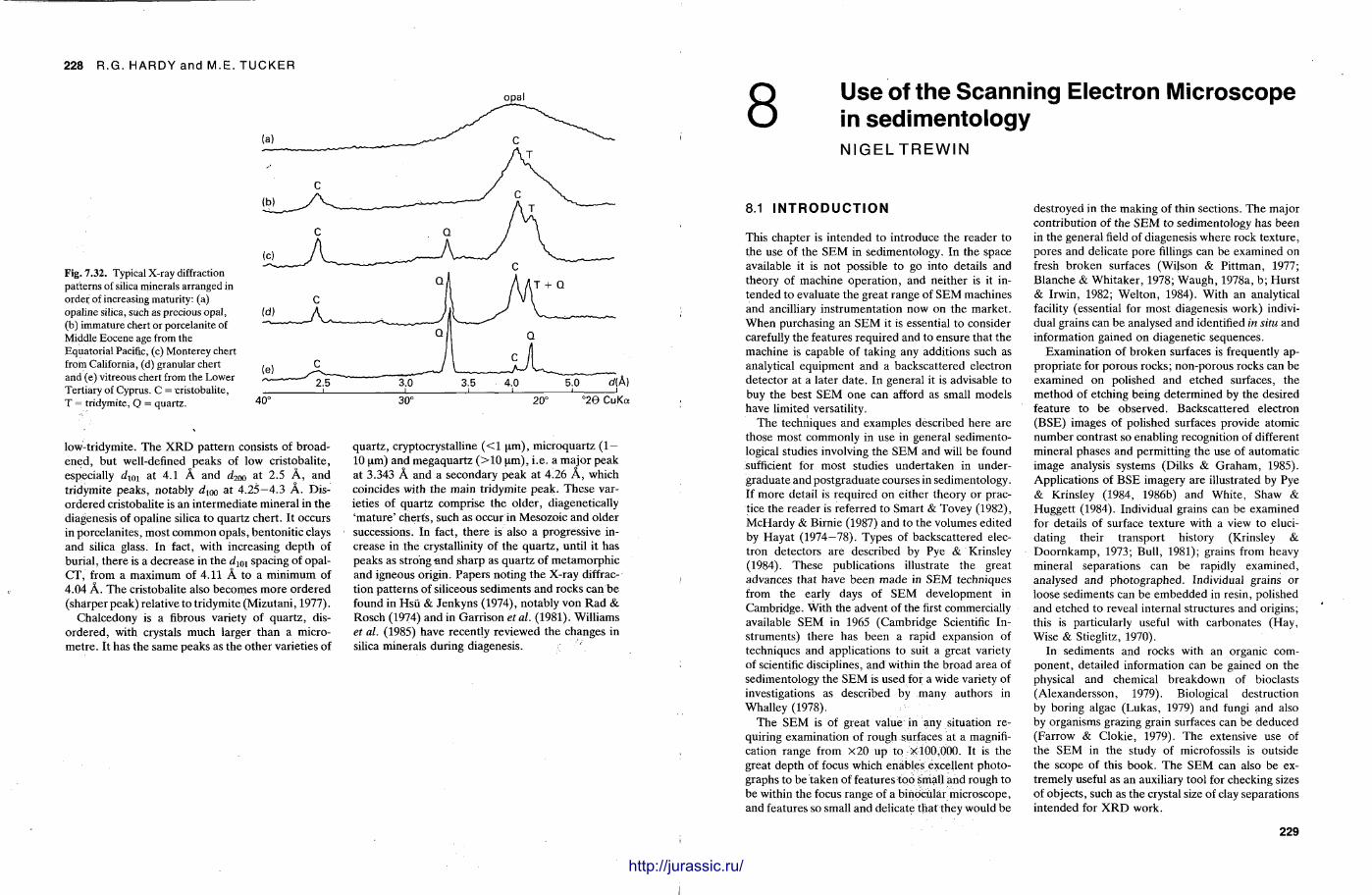
228 R.G. HARDY and M.E. TUCKER
o p a l
Fig. 7.32. Typical X-ray diffraction patterns of silica minerals arranged in order of increasing maturity: (a) opaline silica, such as precious opal, (b) immature chert or porcelanite of Middle Eocene age from the Equatorial Pacific, (c) Monterey chert from California, (d) granular chert and (e) vitreous chert from the Lower Tertiary of Cyprus. C = cristobalite, T = tridymite, Q = quartz.
low-tridymite. T h e X R D pat tern consists of broadened , but well-defined peaks of low cristobalite, especially d10l at 4.1 A and d 2 no at 2.5 A , and tridymite peaks, notably rfion at 4.25—4.3 A . Disordered cristobalite is an intermediate mineral in the diagenesis of opaline silica to quartz chert . It occurs in porcelanites, most common opals, bentonit ic clays and silica glass. In fact, with increasing depth of burial , there is a decrease in the d m spacing of opal-C T , from a maximum of 4.11 A to a minimum of 4.04 A . T h e cristobalite also becomes more ordered (sharper peak) relative to tridymite (Mizutani , 1977).
Chalcedony is a fibrous variety of quar tz , disordered , with crystals much larger than a micromet re . It has the same peaks as the other varieties of
quar tz , cryptocrystalline ( < 1 um) , microquartz (1— 10 um) and megaquar tz ( > 1 0 um) , i.e. a major peak at 3.343 A and a secondary peak at 4.26 A , which coincides with the main tridymite peak. These varieties of quar tz comprise the older , diagenetically 'ma tu re ' cherts , such as occur in Mesozoic and older successions. In fact, there is also a progressive increase in t he crystallinity of the quar tz , until it has peaks as strong a n d sharp as quar tz of metamorphic and igneous origin. Papers noting the X-ray diffraction pat terns of siliceous sediments and rocks can b e found in Hsu & Jenkyns (1974), notably von Rad & Rosch (1974) and in Garrison etal. (1981). Williams et al. (1985) have recently reviewed the changes in silica minerals during diagenesis.
8 Use of the Scanning Electron Microscope in sedimentology NIGELTREWIN
8.1 I N T R O D U C T I O N
This chapter is in tended to introduce the reader to the use of the S E M in sedimentology. In the space available it is not possible to go into details and theory of machine opera t ion , and neither is it intended to evaluate the great range of S E M machines and ancilliary instrumentat ion now on the market . When purchasing an S E M it is essential to consider carefully the features required and to ensure that the machine is capable of taking any additions such as analytical equipment and a backscat tered electron detector at a later da te . In general it is advisable to buy the best S E M one can afford as small models have limited versatility.
The techniques and examples described here are those most commonly in use in general sedimentological studies involving the S E M and will be found sufficient for most studies under taken in undergraduate and postgraduate courses in sedimentology. If more detail is required on either theory or practice the reader is referred to Smart & Tovey (1982), McHardy & Birnie (1987) and to the volumes edited by Hayat (1974—78). Types of backscattered electron detectors are described by Pye & Krinsley (1984). These publications illustrate the great advances that have been made in S E M techniques from the early days of S E M development in Cambridge. With the advent of the first commercially available S E M in 1965 (Cambridge Scientific Instruments) there has been a rapid expansion of techniques and applications to suit a great variety of scientific disciplines, and within the broad area of sedimentology the S E M is used for a wide variety of investigations as described by many authors in Whalley (1978).
The S E M is of great value in any situation requiring examination of rough surfaces at a magnification range from X20 up to x 100.000. It is the great depth of focus which enables excellent photographs to be taken of features too small and rough to be within the focus range of a binocular microscope, and features so small and delicate t h a t they would be
destroyed in the making of thin sections. The major contribution of the S E M to sedimentology has been in the general field of diagenesis where rock texture, pores and delicate pore fillings can be examined on fresh broken surfaces (Wi)son & Pit tman, 1977; Blanche & Whi taker , 1978; Waugh , 1978a, b ; Hurst & Irwin, 1982; Wel ton , 1984). With an analytical facility (essential for most diagenesis work) individual grains can be analysed and identified in situ and information gained on diagenetic sequences.
Examinat ion of b roken surfaces is frequently appropr ia te for porous rocks; non-porous rocks can be examined on polished and etched surfaces, the method of etching being determined by the desired feature to be observed. Backscat tered electron (BSE) images of polished surfaces provide atomic number contrast so enabling recognition of different mineral phases and permitt ing the use of automatic image analysis systems (Dilks & G r a h a m , 1985). Applications of B S E imagery are illustrated by Pye & Krinsley (1984, 1986b) and White , Shaw & Hugget t (1984). Individual grains can be examined for details of surface texture with a view to elucidating their t ransport history (Krinsley & D o o r n k a m p , 1973; Bull, 1981); grains from heavy mineral separations can be rapidly examined, analysed and photographed. Individual grains or loose sediments can be embedded in resin, polished and etched to reveal internal structures and origins; this is particularly useful with carbonates (Hay, Wise & Stieglitz, 1970).
In sediments and rocks with an organic component , detailed information can be gained on the physical and chemical breakdown of bioclasts (Alexandersson, 1979). Biological destruction by boring algae (Lukas , 1979) and fungi and also by organisms grazing grain surfaces can be deduced (Farrow & Clokie, 1979). The extensive use of the S E M in the study of microfossils is outside the scope of this book. The S E M can also be extremely useful as an auxiliary tool for checking sizes of objects, such as the crystal size of clay separations intended for X R D work.
229
JiliJiiJMiMiim http://jurassic.ru/
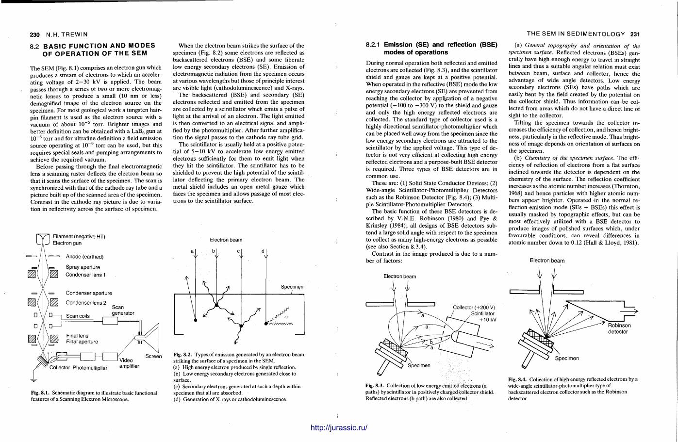
230 N.H. TREWIN
8.2 B A S I C F U N C T I O N A N D M O D E S O F O P E R A T I O N O F T H E S E M
The S E M (Fig. 8.1) comprises an electron gun which produces a stream of electrons to which an accelerating voltage of 2 - 3 0 kV is applied. T h e beam passes through a series of two or more electromagnetic lenses to produce a small (10 nm or less) demagnified image of the electron source on the specimen. For most geological work a tungsten hairpin filament is used as the electron source with a vacuum of about 1 0 - 5 torr . Brighter images and bet ter definition can be obtained with a L a B 6 gun at 1 0 ~ s torr and for ultrafine definition a field emission source operat ing at I O - 9 torr can be used, but this requires special seals and pumping ar rangements to achieve the required vacuum.
Before passing through the final electromagnetic lens a scanning raster deflects the electron beam so that it scans the surface of the specimen. T h e scan is synchronized with that of the cathode ray tube and a picture built up of the scanned area of the specimen. Contras t in the ca thode ray picture is due to variation in reflectivity across the surface of specimen.
When the electron beam strikes the surface of the specimen (Fig. 8.2) some electrons are reflected as backscattered electrons (BSE) and some liberate low energy secondary electrons (SE) . Emission of electromagnetic radiation from the specimen occurs at various wavelengths but those of principle interest are visible light (cathodoluminescence) and X-rays.
The backscattered (BSE) and secondary (SE) electrons reflected and emitted from the specimen are collected by a scintillator which emits a pulse of light at the arrival of an electron. The light emit ted is then converted to an electrical signal and amplified by the photomult ipl ier . After further amplification the signal passes to the cathode ray tube grid.
The scintillator is usually held at a positive potential of 5—10 kV to accelerate low energy emitted electrons sufficiently for them to emit light when they hit the scintillator. T h e scintillator has to be shielded to prevent the high potential of the scintillator deflecting the primary electron beam. The metal shield includes an open metal gauze which faces the specimen and allows passage of most electrons to the scintillator surface.
Filament (negative HT) Electron gun
= Anode (earthed)
Spray aperture ^ Condenser lens 1
Condenser aperture
Condenser lens 2
Scan coils
Scan generator
Video Screen
Collector Photomultiplier amplifier
Fig. 8.1. Schematic diagram to illustrate basic functional features of a Scanning Electron Microscope.
Electron beam
a \
b
\
c d
Specimen /
\ I
Fig. 8.2. Types of emission generated by an electron beam striking the surface of a specimen in the SEM. (a) High energy electron produced by single reflection. (b) Low energy secondary electrons generated close to surface. (c) Secondary electrons generated at such a depth within specimen that all are absorbed. (d) Generation of X-rays or cathodoluminescence.
THE SEM IN SEDIMENTOLOGY 231
8.2.1 Emission (SE) and reflection (BSE) modes of opsrat ions
During normal operat ion both reflected and emitted electrons are collected (Fig. 8.3), and the scintillator shield and gauze are kept at a positive potential . When opera ted in the reflective (BSE) mode the low energy secondary electrons (SE) are prevented from reaching the collector by appljpation of a negative potential (—100 to —300 V) to the shield and gauze and only the high energy reflected electrons are collected. The standard type of collector used is a highly directional scintillator-photomultiplier which can be placed well away from the specimen since the low energy secondary electrons are attracted to the scintillator by the applied voltage. This type of detector is not very efficient at collecting high energy reflected electrons and a purpose-built B S E detector is required. Three types of B S E detectors are in common use.
These are: (1) Solid State Conductor Devices; (2) Wide-angle Scintillator-Photomultiplier Detectors such as the Robinson Detec tor (Fig. 8.4); (3) Multiple Scintillator-Photomultiplier Detectofs .
The basic function of these BSE detectors is described by V . N . E . Robinson (1980) and Pye & Krinsley (1984); all designs of BSE detectors subtend a large solid angle with respect to the specimen to collect as many high-energy electrons as possible (see also Section 8.3.4).
Contrast in the image produced is due to a number of factors:
Electron beam
Fig. 8.3. Collection of low energy emitted electrons (a paths) by scintillator in positively chargedcdlleetor shield. Reflected electrons (b path) are also collected.
(a) General topography and orientation of the specimen surface. Reflected electrons (BSEs) generally have high enough energy to travel in straight lines and thus a suitable angular relation must exist between beam, surface and collector, hence the advantage of wide angle detectors . Low energy secondary electrons (SEs) have paths which are easily bent by the field created by the potential on t he collector shield. Thus information can b e collected from areas which do not have a direct line of sight to the collector.
Tilting the specimen towards the collector increases the efficiency of collection, and hence brightness, particularly in the reflective mode . Thus brightness of image depends on or ientat ion of surfaces on the specimen.
(b) Chemistry of the specimen surface. T h e efficiency of reflection of electrons from a flat surface inclined towards the detector is dependent on the chemistry of the surface. The reflection coefficient increases as t he atomic number increases (Thorn ton , 1968) and hence particles with higher atomic numbers appear brighter. Opera ted in the normal reflection-emission mode (SEs + BSEs) this effect is usually masked by topographic effects, but can be most effectively utilized with a BSE detector to produce images of polished surfaces which, under favourable conditions, can reveal differences in atomic number down to 0.12 (Hall & Lloyd, 1981).
Electron beam
Fig. 8.4. Collection of high energy reflected electrons by a wide-angle scintillator-photomultiplier type of backscattered electron collector such as the Robinson detector.
http://jurassic.ru/
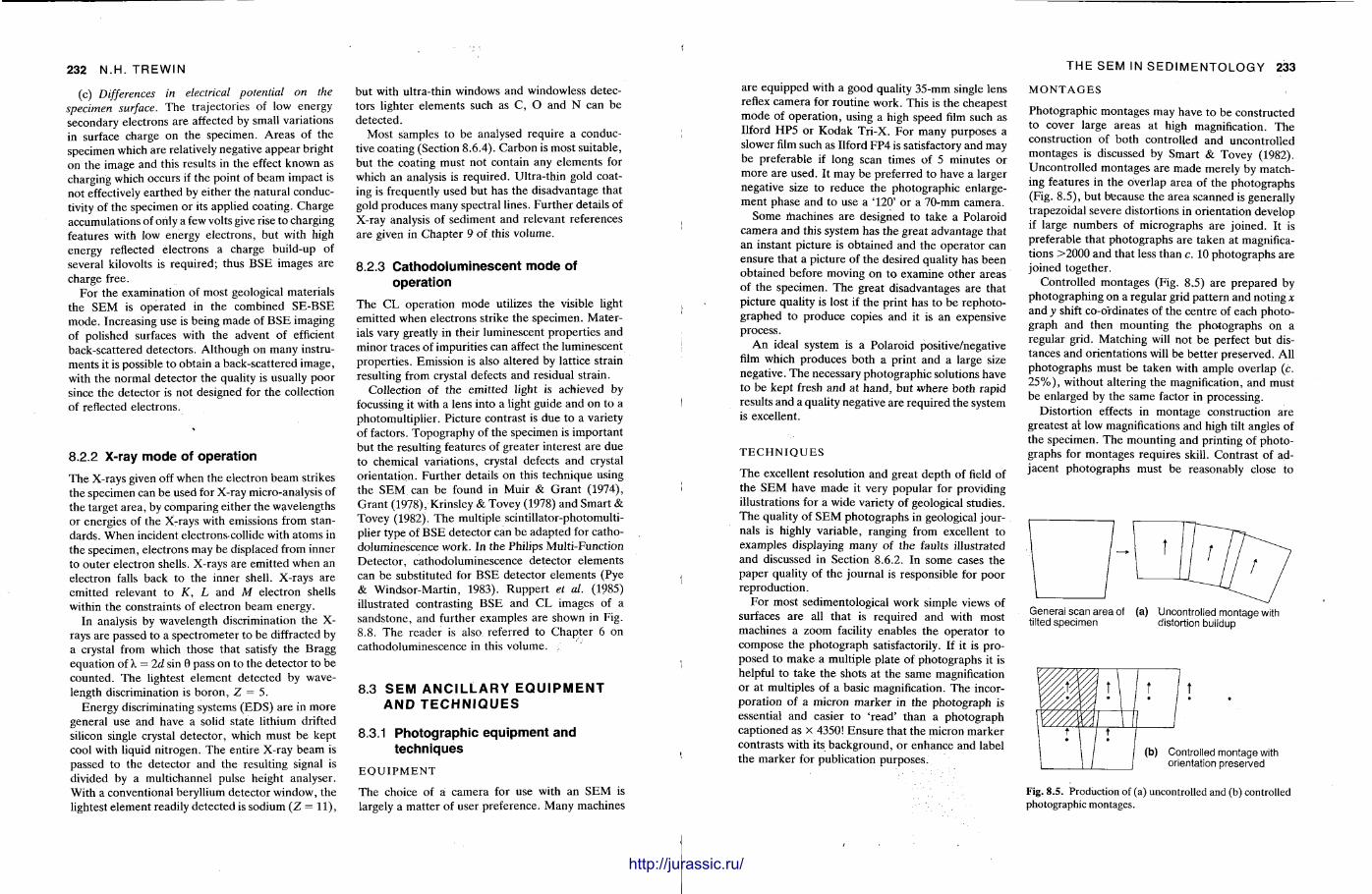
2 3 2 N.H. TREWIN
(c) Differences in electrical potential on the specimen surface. The trajectories of low energy secondary electrons are affected by small variations in surface charge on the specimen. Areas of the specimen which are relatively negative appear bright on the image and this results in the effect known as charging which occurs if the point of beam impact is not effectively ear thed by either the natural conductivity of the specimen o r its applied coating. Charge accumulations of only a few volts give rise to charging features with low energy electrons, but with high energy reflected electrons a charge build-up of several kilovolts is required; thus B S E images are charge free.
For the examination of most geological materials the S E M is opera ted in the combined SE-BSE mode . Increasing use is being made of B S E imaging of polished surfaces with the advent of efficient back-scattered detectors . Al though on many instruments it is possible to obtain a back-scattered image, with the normal detector the quality is usually poor since the detector is not designed for the collection of reflected electrons.
8.2.2 X-ray mode of operation
The X-rays given off when the electron beam strikes the specimen can be used for X-ray micro-analysis of the target area , by comparing either the wavelengths or energies of the X-rays with emissions from standards . When incident electrons-collide with a toms in the specimen, electrons may be displaced from inner to outer electron shells. X-rays are emitted when an electron falls back to the inner shell. X-rays are emitted relevant to K, L and M electron shells within the constraints of electron beam energy.
In analysis by wavelength discrimination the X-rays are passed to a spectrometer to be diffracted by a crystal from which those that satisfy the Bragg equation of X = 2d sin 6 pass on to the detector to be counted . T h e lightest e lement detected by wavelength discrimination is boron , Z = 5.
Energy discriminating systems (EDS) are in more general use and have a solid state lithium drifted silicon single crystal detector , which must be kept cool with liquid nitrogen. The entire X-ray beam is passed to the detector and the resulting signal is divided by a multichannel pulse height analyser. With a conventional beryllium detector window, the lightest e lement readily detected is sodium ( Z = 11),
but with ultra-thin windows and windowless detectors lighter e lements such as C, O and N can be detected.
Most samples to be analysed require a conductive coating (Section 8.6.4). Carbon is most suitable, but the coating must not contain any elements for which an analysis is required. Ultra-thin gold coating is frequently used but has the disadvantage that gold produces many spectral lines. Fur ther details of X-ray analysis of sediment and relevant references are given in Chap te r 9 of this volume.
8.2.3 Cathodoluminescent mode of operation
T h e C L operat ion mode utilizes the visible light emitted when electrons strike the specimen. Materials vary greatly in their luminescent proper t ies and minor traces of impurities can affect the luminescent propert ies . Emission is also altered by lattice strain resulting from crystal defects and residual strain.
Collection of the emitted light is achieved by focussing it with a lens into a light guide and on to a photomultiplier . Picture contrast is due to a variety of factors. Topography of the specimen is impor tant but the resulting features of greater interest are due to chemical variations, crystal defects and crystal or ientat ion. Fur ther details on this technique using the S E M can be found in Muir & Gran t (1974), Gran t (1978), Krinsley & Tovey (1978) and Smart & Tovey (1982). T h e multiple scintillator-photomulti-plier type of BSE detector can be adapted for cathodoluminescence work. In the Philips Multi-Function Detec tor , cathodoluminescence detector e lements can be substituted for BSE detector e lements (Pye & Windsor-Mart in , 1983). Rupper t et al. (1985) illustrated contrasting B S E and C L images of a sandstone, and further examples are shown in Fig. 8.8. The reader is also referred to Chapter 6 on cathodoluminescence in this volume.
8.3 S E M A N C I L L A R Y E Q U I P M E N T A N D T E C H N I Q U E S
8.3.1 Photographic equipment and techniques
E Q U I P M E N T
The choice of a camera for use with an S E M is largely a mat ter of user preference. Many machines
THE SEM IN SEDIMENTOLOGY 233
are equipped with a good quality 35-mm single lens reflex camera for rout ine work. This is t he cheapest m o d e of operat ion, using a high speed film such as Uford H P 5 or Kodak Tri-X. For many purposes a slower film such as Ilford FP4 is satisfactory and may be preferable if long scan times of 5 minutes or more are used. It may be preferred to have a larger negative size to reduce the photographic enlargement phase and to use a '120' or a 70-mm camera.
Some machines are designed to take a Polaroid camera and this system has the great advantage that an instant picture is obtained and the opera tor can ensure that a picture of the desired quality has been obtained before moving on to examine other areas of the specimen. The great disadvantages are that picture quality is lost if the print has to be rephoto-graphed to produce copies and it is an expensive process.
A n ideal system is a Polaroid positive/negative film which produces both a print and a large size negative. The necessary photographic solutions have to be kept fresh and at hand , but where both rapid results and a quality negative are required the system is excellent.
T E C H N I Q U E S
The excellent resolution and great depth of field of the S E M have m a d e it very popular for providing illustrations for a wide variety of geological studies. T h e quality of S E M photographs in geological journals is highly variable, ranging from excellent to examples displaying many of the faults illustrated and discussed in Section 8.6.2. In some cases the paper quality of the journal is responsible for poor reproduct ion.
For most sedimentological work simple views of surfaces are all that is required and with most machines a zoom facility enables the opera tor to compose the photograph satisfactorily. If it is proposed to m a k e a multiple plate of photographs it is helpful to take the shots at the same magnification or at multiples of a basic magnification. The incorporat ion of a micron marker in the photograph is essential and easier to ' read ' than a photograph captioned as x 4350! Ensure that the micron marker contrasts with its background, or enhance and label the marker for publication purposes .
M O N T A G E S
Photographic montages may have to be constructed to cover large areas at high magnification. The construction of both controlled and uncontrolled montages is discussed by Smart & Tovey (1982). Uncontrol led montages a re m a d e merely by matching features in the overlap area of the photographs (Fig. 8.5), but because the area scanned is generally trapezoidal severe distortions in orientation develop if large numbers of micrographs a re joined. It is preferable that photographs are taken at magnifications >2000 and that less than c. 10 photographs are joined together .
Control led montages (Fig. 8.5) are prepared by photographing on a regular grid pat tern and noting x a n d y shift co-ordinates of the centre of each photograph and then mounting the photographs on a regular grid. Matching will not be perfect but distances and orientat ions will be bet ter preserved. All photographs must be taken with ample overlap (c. 2 5 % ) , without altering the magnification, and must be enlarged by the same factor in processing.
Distort ion effects in montage construction are greatest at low magnifications and high tilt angles of the specimen. The mount ing and printing of photographs for montages requires skill. Contrast of adjacent photographs must be reasonably close to
General scan area of (a) Uncontrolled montage with tilted specimen distortion buildup
(b) Controlled montage with orientation preserved
Fig. 8.5. Production of (a) uncontrolled and (b) controlled photographic montages.
11111 HitMlitljjjitlih'llMlMJitiT̂™ http://jurassic.ru/
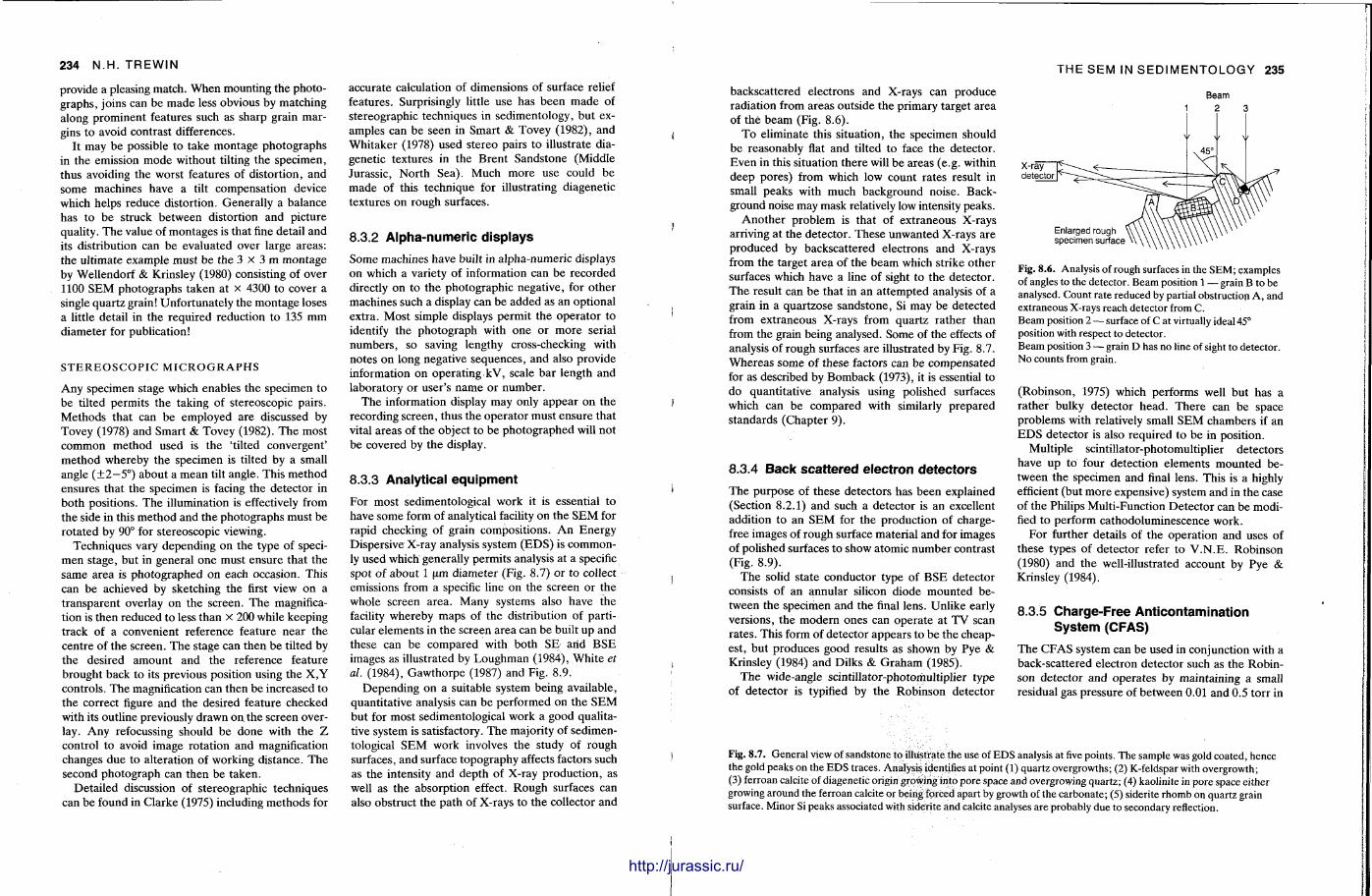
234 N . H . T R E W I N
provide a pleasing match. When mounting the photographs, joins can be m a d e less obvious by matching along prominent features such as sharp grain margins to avoid contrast differences.
It may be possible to take montage photographs in the emission mode without tilting the specimen, thus avoiding the worst features of distort ion, and some machines have a tilt compensat ion device which helps reduce distortion. General ly a balance has to be struck between distortion and picture quality. The value of montages is that fine detail and its distribution can be evaluated over large areas: the ult imate example must be the 3 x 3 m montage by Wellendorf & Krinsley (1980) consisting of over 1100 S E M photographs taken at x 4300 to cover a single quar tz grain! Unfortunately the montage loses a little detail in the required reduction to 135 m m diameter for publication!
S T E R E O S C O P I C M I C R O G R A P H S
Any specimen stage which enables the specimen to be tilted permits the taking of stereoscopic pairs. Methods that can be employed are discussed by Tovey (1978) and Smart & Tovey (1982). T h e most common method used is the 'tilted convergent ' method whereby the specimen is tilted by a small angle (±2—5°) about a mean tilt angle. This method ensures that the specimen is facing the detector in both positions. The illumination is effectively from the side in this method and the photographs must be rotated by 90° for stereoscopic viewing.
Techniques vary depending on the type of specimen stage, but in general one must ensure that the same area is photographed on each occasion. This can be achieved by sketching the first view on a t ransparent overlay on the screen. T h e magnification is then reduced to less than x 200 while keeping track of a convenient reference feature near the centre of the screen. T h e stage can then be tilted by the desired amount and the reference feature brought back to its previous position using the X , Y controls. The magnification can then be increased to the correct figure and the desired feature checked with its outline previously drawn on the screen overlay. Any refocussing should be done with the Z control to avoid image rotat ion and magnification changes due to alteration of working distance. T h e second photograph can then be taken .
Detai led discussion of stereographic techniques can be found in Clarke (1975) including methods for
accurate calculation of dimensions of surface relief features. Surprisingly little use has been made of stereographic techniques in sedimentology, but examples can be seen in Smart & Tovey (1982), and Whi taker (1978) used stereo pairs to illustrate diagenetic textures in the Brent Sandstone (Middle Jurassic, Nor th Sea) . Much more use could be made of this technique for illustrating diagenetic textures on rough surfaces.
8.3.2 Alpha-numeric displays
Some machines have built in alpha-numeric displays on which a variety of information can be recorded directly on to the photographic negative, for o ther machines such a display can be added as an optional extra. Most simple displays permit the opera tor to identify the photograph with one or more serial numbers , so saving lengthy cross-checking with notes on long negative sequences, and also provide information on operat ing kV, scale bar length and laboratory or user 's name or number .
T h e information display may only appear on the recording screen, thus the opera tor must ensure that vital areas of the object to be photographed will not be covered by the display.
8.3.3 Analytical equipment
For most sedimentological work it is essential to have some form of analytical facility on the S E M for rapid checking of grain composit ions. A n Energy Dispersive X-ray analysis system (EDS) is commonly used which generally permits analysis at a specific spot of about 1 um diameter (Fig. 8.7) or to collect emissions from a specific line on the screen or the whole screen area. Many systems also have the facility whereby maps of the distribution of particular elements in the screen area can be built up and these can be compared with both SE arid B S E images as illustrated by Loughman (1984), Whi te et al. (1984), Gawthorpe (1987) and Fig. 8.9.
Depending on a suitable system being available, quanti tat ive analysis can be performed on the S E M but for most sedimentological work a good qualitative system is satisfactory. T h e majority of sedimentological S E M work involves the study of rough surfaces, and surface topography affects factors such as the intensity and depth of X-ray product ion, as well as the absorption effect. Rough surfaces can also obstruct the path of X-rays to the collector and
T H E S E M I N S E D I M E N T O L O G Y 235
backscattered electrons and X-rays can produce radiation from areas outside the primary target area of the beam (Fig. 8.6).
T o eliminate this si tuation, the specimen should be reasonably flat and tilted to face the detector . Even in this situation there will be areas (e.g. within deep pores) from which low count rates result in small peaks with much background noise. Background noise may mask relatively low intensity peaks.
A n o t h e r problem is that of ext raneous X-rays arriving at the detector . These unwanted X-rays are produced by backscattered electrons and X-rays from the target area of the beam which strike other surfaces which have a line of sight to the detector . T h e result can be that in an a t tempted analysis of a grain in a quartzose sandstone, Si may be detected from extraneous X-rays from quartz ra ther than from the grain being analysed. Some of the effects of analysis of rough surfaces are illustrated by Fig. 8.7. Whereas some of these factors can be compensated for as described by Bomback (1973), it is essential to do quanti tat ive analysis using polished surfaces which can be compared with similarly prepared s tandards (Chapter 9) .
8.3.4 Back scattered electron detectors
T h e purpose of these detectors has been explained (Section 8.2.1) and such a detector is an excellent addition to an S E M for the product ion of charge-free images of rough surface material and for images of polished surfaces to show atomic number contrast (Fig. 8.9).
The solid state conductor type of B S E detector consists of an annular silicon diode mounted between the specimen and the final lens. Unl ike early versions, the modern ones can opera te at T V scan rates . This form of detector appears to be the cheapest, but produces good results as shown by Pye & Krinsley (1984) and Dilks & G r a h a m (1985).
The wide-angle scintillator-photomultiplier type of detector is typified by the Robinson detector
Enlarged rough specimen surface
Fig. 8 .6 . Analysis of rough surfaces in the SEM; examples of angles to the detector. Beam position 1 — grain B to be analysed. Count rate reduced by partial obstruction A, and extraneous X-rays reach detector from C. Beam position 2 — surface of C at virtually ideal 45° position with respect to detector. Beam position 3 — grain D has no line of sight to detector. No counts from grain.
(Robinson, 1975) which performs well but has a ra ther bulky detector head . The re can be space problems with relatively small S E M chambers if an E D S detector is also required to be in position.
Multiple scintillator-photomultiplier detectors have up to four detection elements mounted between the specimen and final lens. This is a highly efficient (but more expensive) system and in the case of the Philips Multi-Function Detec tor can be modified to perform cathodoluminescence work.
For further details of the operat ion and uses of these types of detector refer to V . N . E . Robinson (1980) and the well-illustrated account by Pye & Krinsley (1984).
8.3.5 Charge-Free Ant icontaminat ion System (CFAS)
The C F A S system can be used in conjunction with a back-scattered electron detector such as the Robinson detector and opera tes by maintaining a small residual gas pressure of between 0.01 and 0.5 torr in
Fig. 8 .7 . General view of sandstone to illustrate the use of EDS analysis at five points. The sample was gold coated, hence the gold peaks on the EDS traces. Analysis identifies at point (1) quartz overgrowths; (2) K-feldspar with overgrowth; (3) ferroan calcite of diagenetic origin growing into pore space and overgrowing quartz; (4) kaolinite in pore space either growing around the ferroan calcite or being forced apart by growth of the carbonate; (5) siderite rhomb on quartz grain surface. Minor Si peaks associated with siderite and calcite analyses are probably due to secondary reflection.
liiil nil ii http://jurassic.ru/
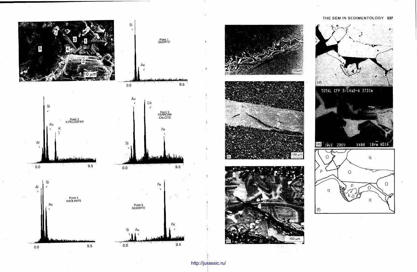
THE SEM IN SEDIMENTOLOGY 237
http://jurassic.ru/
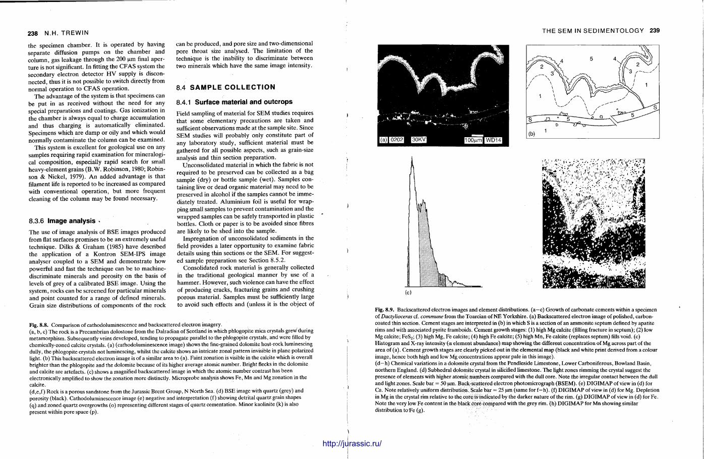
238 N .H . T R E W I N
the specimen chamber . It is opera ted by having separate diffusion pumps on the chamber and column, gas leakage through the 200 um final aperture is not significant. In fitting the C F A S system the secondary electron detector H V supply is disconnected, thus it is not possible to switch directly from normal operat ion to C F A S operat ion.
The advantage of the system is that specimens can be put in as received without the need for any special preparat ions and coatings. Gas ionization in the chamber is always equal to charge accumulation and thus charging is automatically el iminated. Specimens which are d a m p or oily and which would normally contaminate the column can be examined.
This system is excellent for geological use on any samples requiring rapid examination for mineralogical composit ion, especially rapid search for small heavy-element grains (B .W. Robinson, 1980; Robinson & Nickel, 1979). A n added advantage is that filament life is repor ted to be increased as compared with conventional operat ion, but more frequent cleaning of the column may be found necessary.
8.3.6 Image analysis •
The use of image analysis of B S E images produced from flat surfaces promises to be an extremely useful technique. Dilks & G r a h a m (1985) have described the application of a Kont ron SEM-IPS image analyser coupled to a S E M and demonst ra te how powerful and fast the technique can be to machine-discriminate minerals and porosity on the basis of levels of grey of a calibrated B S E image. Using the system, rocks can be screened for particular minerals and point counted for a range of defined minerals . Grain size distributions of components of the rock
can be produced , and pore size and two-dimensional pore throat size analysed. T h e limitation of the technique is the inability to discriminate be tween two minerals which have the same image intensity.
8.4 S A M P L E C O L L E C T I O N
8.4.1 Surface material and outcrops
Field sampling of mater ial for S E M studies requires that some elementary precautions are taken and sufficient observations made at the sample site. Since S E M studies will probably only constitute part of any laboratory s tudy, sufficient material must be gathered for all possible aspects, such as grain-size analysis and thin section preparat ion.
Unconsol idated material in which the fabric is not required to be preserved can be collected as a bag sample (dry) or bott le sample (wet) . Samples containing live or dead organic material may need to be preserved in alcohol if the samples cannot be immediately t rea ted . Aluminium foil is useful for wrapping small samples to prevent contaminat ion and the wrapped samples can be safely t ranspor ted in plastic bottles. Cloth or paper is to be avoided since fibres are likely to be shed into the sample.
Impregnat ion of unconsolidated sediments in the field provides a later opportuni ty to examine fabric details using thin sections or the S E M . For suggested sample prepara t ion see Section 8.5.2.
Consolidated rock mater ial is generally collected in the traditional geological manner by use of a hammer . However , such violence can have the effect of producing cracks, fracturing grains and crushing porous material . Samples must be sufficiently large to avoid such effects and (unless it is the object of
Fig. 8.8. Comparison of cathodoluminescence and backscattered electron imagery. (a, b, c) The rock is a Precambrian dolostone from the Dalradian of Scotland in which phlogopite mica crystals grew during metamorphism. Subsequently veins developed, tending to propagate parallel to the phlogopite crystals, and were filled by chemically-zoned calcite crystals, (a) (cathodoluminescence image) shows the fine-grained dolomite host-rock luminescing dully, the phlogopite crystals not luminescing, whilst the calcite shows an intricate zonal pattern invisible in plane polarized light, (b) This backscattered electron image is of a similar area to (a). Faint zonation is visible in the calcite which is overall brighter than the phlogopite and the dolomite because of its higher average atomic number. Bright flecks in the dolomite and calcite are artefacts, (c) shows a magnified backscattered image in which the atomic number contrast has been electronically amplified to show the zonation more distinctly. Microprobe analysis shows Fe, Mn and Mg zonation in the calcite. (d,e,f) Rock is a porous sandstone from the Jurassic Brent Group, N North Sea. (d) BSE image with quartz (grey) and porosity (black). Cathodoluminescence image (e) negative and interpretation (f) showing detrital quartz grain shapes (q) and zoned quartz overgrowths (o) representing different stages of quartz cementation. Minor kaolinite (k) is also present within pore space (p).
T H E S E M IN S E D I M E N T O L O G Y 239
(c)
Fig. 8.9. Backscattered electron images and element distributions, (a—c) Growth of carbonate cements within a specimen of Dactylioceras cf. commune from the Toarcian of NE Yorkshire, (a) Backscattered electron image of polished, carbon-coated thin section. Cement stages are interpreted in (b) in which S is a section of an ammonite septum defined by apatite rims and with associated pyrite framboids. Cement growth stages: (1) high Mg calcite (filling fracture in septum); (2) low Mg calcite; FeS 2 ; (3) high Mg, Fe calcite; (4) high Fe calcite; (5) high Mn, Fe calcite (replaces septum) fills void, (c) Histogram and X-ray intensity (a element abundance) map showing the different concentration of Mg across part of the area of (a). Cement growth stages are clearly picked out in the elemental map (black and white print derived from a colour image, hence both high and low Mg concentrations appear pale in this image). (d—h) Chemical variations in a dolomite crystal from the Pendleside Limestone, Lower Carboniferous, Bowland Basin, northern England, (d) Subhedral dolomite crystal in silicified limestone. The light zones rimming the crystal suggest the presence of elements with higher atomic: numbers compared with the dull core. Note the irregular contact between the dull and light zones. Scale bar = 50 \ t m . Back-scattered electron photomicrograph (BSEM). (e) DIGIMAP of view in (d) for Ca. Note relatively uniform distribution. Scale bar = 25 \ i m (same for f -h ) . (f) DIGIMAP of view in (d) for Mg. Depletion in Mg in the crystal rim relative to the corgis-indicated by the darker nature of the rim. (g) DIGIMAP of view in (d) for Fe. Note the very low Fe content in the black core compared with the grey rim. (h) DIGIMAP for Mn showing similar distribution to Fe (g).
http://jurassic.ru/
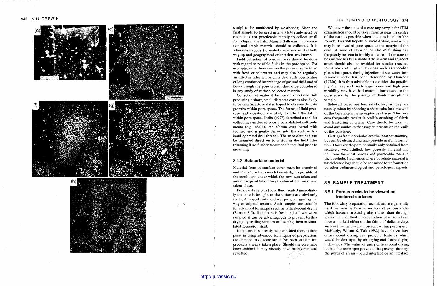
240 N.H. TREWIN THE SEM IN SEDIMENTOLOGY 241
study) to be unaffected by weathering. Since the final sample to be used in any S E M study must be clean it is not practicable merely to collect small rock chips in the field. Many pitfalls exist in preparation and ample material should be collected. It is advisable to collect oriented specimens so that both way-up and geographical orientation are known.
Field collection of porous rocks should be done with regard to possible fluids in the pore space. For example , on a shore section the pores may be filled with fresh or salt water and may also be regularly air-filled as tides fall or cliffs dry. Such possibilities of long continued interchange of gas and fluid and of flow through the pore system should be considered in any study of surface collected material .
Collection of material by use of a por table drill producing a short , small d iameter core is also likely to be unsatisfactory if it is hoped to observe delicate growths within pore space. The forces of fluid pressure and vibration are likely to affect the fabric within pore space. Joslin (1977) described a tool for collecting samples of poorly consolidated soft sediments (e.g. chalk). A n 80-mm core barrel with toothed end is gently drilled into the rock with a hand opera ted drill (brace) . The core obtained can be mounted direct on to a stub in the field after tr imming if no further t rea tment is required prior to mounting.
8.4.2 Subsurface material
Material from subsurface cores must be examined and sampled with as much knowledge as possible of the conditions under which the core was taken and any subsequent laboratory t rea tment that may have taken place.
Preserved samples (pore fluids sealed immediately the core is brought to the surface) are obviously the best to work with and will preserve most in the way of original texture . Such samples are suitable for advanced techniques such as critical-point drying (Section 8.5). If the core is fresh and still wet when sampled it can be advantageous to prevent further drying by sealing samples or keeping them in simulated formation fluid.
If the core has already been air dried there is little point in using advanced techniques of prepara t ion; the damage to delicate structures such as illite has probably already taken place. Should the core have been slabbed it may already have Been dried and rewetted.
Whatever the state of a core any sample for S E M examination should be taken from as near the centre of the core as possible when the core is still in ' the round ' . This will hopefully avoid drilling mud which may have invaded pore space at the margin of the core. A zone of invasion or else of flushing can frequently be seen in freshly cut cores. If the core to be sampled has been slabbed the sawcut and adjacent areas should also be avoided for similar reasons. Penetra t ion of organic material such as coccolith plates into pores during injection of sea water into reservoir rocks has been described by Hancock (1978a); it is thus advisable to consider the possibility that any rock with l a rge pores and high permeability may have had material introduced to the pore space by the passage of fluids through the sample.
Sidewall cores are less satisfactory as they are usually taken by shooting a short tube into the wall of the borehole with an explosive charge. This process frequently results in visible crushing of fabric and fracturing of grains. Care should be taken to avoid any mudcake that may be present on the walls of the borehole .
Cuttings from boreholes are the least satisfactory, but can be cleaned and may provide useful information. However they are normally only obtained from relatively well lithified, low porosity material and not from the most porous and permeable rocks in the borehole . In all cases where borehole material is used electric logs should be consulted for information on other sedimentological and petrological aspects.
8.5 S A M P L E T R E A T M E N T
8.5.1 Porous rocks to be viewed on fractured surfaces
The following preparat ion techniques are generally used for viewing broken surfaces of porous rocks which fracture around grains ra ther than through grains. T h e method of preparat ion of material can have a marked effect on the fabric of delicate clays such as filamentous illite present within pore space. McHardy , Wilson & Tait (1982) have shown how critical-point drying can preserve features which would be destroyed by air-drying and freeze-drying techniques. The value of using critical-point drying is that the technique prevents the passage through the pores of an air—liquid interface or an interface
http://jurassic.ru/
242 N.H. TREWIN
between immiscible liquids. It is the passage of such an interface which can cause collapse and reorientation of clays within pore space. If it is known that the specimen has already been air dried, advanced techniques of preparat ion cannot restore the situation. Fur ther useful details of preparat ion techniques for clays are given by McHardy & Birnie (1987).
A I R - D R I E D S A M P L E S
Samples previously air dried and which contained water as the pore fluid can be examined without further t rea tment , but it is frequently advisable to wash the specimen with distilled water to remove any chlorides or other soluble salts which may have crystallized in pore space due to the evaporat ion of saline pore water . This is best achieved by soaking a sample, not more than 1 cm thick, in distilled water until it is chloride free. (The time taken will depend on permeabili ty and salinity of the evaporated pore water . ) This technique is also useful for mode rn marine sediments and rock material collected from shore sections.
Air drying, combined with removal of water soluble material , is also a technique which can be used to study the soluble salts and the effects of their removal . This has applications in the study of weathering of rocks and the formation of evapori tes.
If delicate material such as fibrous illite is suspected to exist in pore space and either t ime or lack of apparatus precludes use of critical-point drying, better results may be obtained by air drying samples from amyl acetate . T h e advantage of this method is that amyl acetate has a much lower surface tension than water and so the forces exerted at the liquid— gas interface as the specimen dries are reduced.
O I L - S A T U R A T E D S A M P L E S
Rocks that are oil-saturated, or which contain oil residues after evaporat ion of lighter hydrocarbons , must have the hydrocarbon removed prior to S E M examinat ion. If oil is not removed it is vaporized by the electron beam and will make the S E M column dirty and reduce picture quality. Oil also prevents the efficient coating of the sample with gold, resulting in charging of the specimen and poor resolution pictures.
Oil can be removed by use of solvents such as acetone, xylene, to luene , chloroform and trichlo-roe thane . Chloroform and t r ichloroethane are the
most efficient at removing oil. It is possibly safer to use t r ichloroethane than chloroform, but full safety precautions (gloves and fume cupboard) should be taken in handling all these solvents.
Method. A sample measuring about 10 x 10 x 5 mm is immersed in the solvent and sealed in an airtight jar ( to prevent fumes). The solvent is changed every 12 hours . T h e process is repea ted until all the oil has been removed; this can be judged by lack of a residual oil film on evaporat ion of a few drops of the used solvent on a glass slide. With reasonably permeable rocks two changes of t r ichloroethane are normally sufficient to remove the oil. T h e sample is then allowed to air dry at room tempera ture for 24 hours . If residual oil appears on the specimen surface after drying, a final washing in solvent will usually remove the last traces. A fresh fracture surface can then be produced for observation in the S E M . Comparisons of oil saturated and oil-free samples t reated by the above method show no apparent difference in clay morphology or orientat ion.
Removal of oil from rocks with poor permeabil i ty can be exceedingly difficult and the samples may have to be flushed of oil by application of a pressure difference across the sample. Oil can be t rapped in pores which are no longer connected, and in cases such as this only the surface of the sample can be effectively cleaned and only small specimens should be used to minimize the amount of oil that may be released from the rock when under vacuum in the S E M chamber:
In commercial core analysis laboratories oil is frequently removed using a Soxhlet extractor. The sample is first flushed with methanol to remove water , a process which may take from 8 hours to 3 days depending on permeabil i ty. T h e sample is then dried in air until the bulk of the methanol has evaporated and then put back in another extractor with xylene or to luene and flushed until clean. Cleanliness is generally judged by a lack of fluorescence under U V light. The sample can then be air dried as required. There is the possibility that the more active flushing in this method and the in termediate drying stage could affect clay fabrics.
Drying of wet specimens can be accomplished at room tempera ture , by use of an oven or by application of a vacuum. All these methods involve a volume decrease of clay or mud specimens with the result that depositional textures of clays are probably not retained. If specimens are oven dried, a low tempera ture (50°C) should be used to avoid loss of
Hi
THE SEM IN SEDIMENTOLOGY 243
structural water in clays. If washed cuttings from oil wells are being examined it is essential to ensure that the cuttings were not dried at a high tempera ture after the washing process.
F R E E Z E D R Y I N G
Freeze-drying techniques are used extensively on biological material and have been applied successfully to clay—water systems in soils. This method is favoured by Ero l , Lohnes & Demire l (1976) for preparat ion of swelling clays such as Na-montmori l -lonites. It does not involve replacement of water with an organic liquid which could cause swelling and ion exchange in the clays.
Method. The method described by McHardy et al. (1982) used 10-mm pieces of rock (Jurassic, Magnus Field reservoir from the North Sea) which were either directly frozen with the contained pore water or frozen after the samples were washed free of chloride. Samples were plunged into liquid nitrogen or freon for at least 30 minutes , they were then vacuum-dried from the frozen state in an Edwards Modulyo freeze-drier. The drying phase takes several days.
For the method to be a success the specimen must be cooled very rapidly so that the water is frozen in place and ice crystals do not form. The rate of cooling required is several hundred degrees per second and this will only be accomplished on the outer surface of the rock, and possibly to a depth of only 0.1 m m (Greene-Kelly, 1973). Ano the r problem is encountered in the drying phase when it is necessary to warm the specimen to a tempera ture greater than — 40°C to achieve sublimation of the ice in a reasonable t ime, but at this tempera ture rapid growth of ice crystals will occur which will displace matrix clays.
The main applications of freeze-drying of samples are in the study of soils and swelling clays. McHardy et al. (1982) found this method inferior to critical-point drying for preservation of delicate illite in pore space.
C R I T I C A L - P O I N T D R Y I N G
The advantage of the critical-point drying technique is that it eliminates the surface-tension forces applied to delicate crystals during the drying stage by avoiding the passage of an air—water interface
through the pore space. This results in bet ter preservation of delicate structures, such as fibrous illite (McHardy et al., 1982). Tovey & Wong (1978) favoured this method for the preparat ion of wet sediment samples. The disadvantage of the method is that it is t ime-consuming, requires special apparatus, and has disadvantages if swelling clays are present (see above) .
The method of preparat ion used by McHardy et al. (1982) is as follows. Pieces of rock of 10-mm size which contained simulated formation water had the water replaced by methanol by the successive passage through the specimens of 1:3, 1:1 and 3:1 methanol—water mixtures and finally 100% methanol. The methanol was then replaced daily until free from chloride which was taken to indicate that all po re fluid had been replaced by methanol . T h e samples were then transferred to the critical-point drying apparatus (Polaron model E3000 with a liquid transfer boat with integral drain valve). The boat with six to eight samples in methanol was loaded into the pressure chamber which was pre-cooled by cold mains water . The chamber was flushed with liquid CO2 for about 10 min and allowed to stand for several hours with the C 0 2 level above the samples at all t imes. T o ensure replacement of methanol by liquid C 0 2 the chamber was flushed with C 0 2 for 5—10 min twice a day for a week. Finally the pressure apparatus was heated to 37°C by water circulation from a 40° thermosta t to bring it above the critical point of C 0 2 (32°C) and the tempera ture held for 30 min to ensure equilibrium was reached in the samples. T h e C 0 2 was then slowly vented from the chamber at 2 ml s - 1 which was slow enough to prevent condensat ion of C 0 2 in the chamber . The dried samples were then ready for production of a clean fracture face and mount ing as described below in Section 8.6.
Critical-point drying has been found useful for the t rea tment of illite-bearing sandstones (McHardy et al., 1982; McHardy & Birnie, 1987) and has also been used in studies on pore-size distribution in soils (Lawrence, 1977; Murray & Quirk, 1980) and should be considered as a preparat ion method well worth trying with porous samples that have their original pore fluids preserved. Farrow & Clokie (1979) used critical-point drying in a study of boring algae to reveal algal filaments within the borings. The samples were first fixed with glutaraldehyde, dehydrated through a series of alcohols and brought to acetone and then critically point dried.
http://jurassic.ru/
244 N.H. TREWIN
8.5.2 Non-porous rocks
Rocks which have low porosity or in which grains and cement give similar resistance to fracturing, as is the case in many quartz-cemented sandstones and well-cemented limestones or dolomites, may not reveal much information when rough broken surfaces are examined. In such cases it is frequently necessary to view a polished and etched surface to obtain useful information.
This technique is particularly useful in the examination of carbonate cemented sandstones, limestones and dolomites , since by suitable choice of etching agent different minerals can be at tacked and their role as grains or cement elucidated. The technique can also be used on unconsolidated sediments which have been resin-impregnated in the field or laboratory.
G E N E R A L M E T H O D S
A slice of the rock to be examined is cut to a suitable thickness (say 3—5 m m ) . T h e specimen can thus be oriented in any required manner and part of the rock slice used to make a thin section or polished section for examination by other techniques.
The rock slice or chip should be polished to a reasonable s tandard with respect to the features required to the viewed (polishing details in Lister, 1978). The specimen slice should be cut or b roken to the required size for insertion in the S E M chamber and mounted on the stub prior to etching to minimize the possibility of damage to the delicate etched surface. Some S E M chambers will accommodate a polished thin-section; this enables the same area to be examined using a variety of techniques and is an obvious advantage.
The etching process can be varied to suit the particular situation. For l imestones, dilute hydrochloric, acetic or formic acid can be used for low-relief etching. It is best to use as dilute a solution as possible to avoid vigorous gas generat ion which could damage delicate features. Sandberg & Hudson (1983) used 0 .25% formic acid and an etch time of 60—90 s to reveal aragonite relics in calcite-replaced shells. Hay et al. (1970) used 1% HC1 and found 30 s of etching sufficient to reveal the ul trastructure of fine carbonate grains of biogenic origin. Despi te the above examples of gentle etching, Wilkinson, Janecke & Brett (1982) used 5 0 % glacial acetic acid
and an etch time of 60 s with success on Ordovician l imestones.
D e e p etching can be employed profitably in rocks with a soluble cement. A calcite-cemented sandstone can be etched down from a flat broken surface to reveal the pre-cement morphology and to observe relics of carbonate replaced grains. Thus it is possible by use of suitable acids to manufacture examples of secondary porosity in carbonate cemented rocks. Particularly interesting results can be achieved with dolomite/calcife rocks and partially silicified limestones. It is useful to prepare a number of stubs of each rock to be examined so that ample material is available for experimentat ion with different acids and etch times. In this way photographs can be taken of examples 'before ' and 'after' t rea tment . Polished surfaces of quartzitic sandstones can be etched with hydrofluoric acid to reveal rock texture and internal structures of grains such as heavy minerals.
With all etching techniques the specimen must be well washed with distilled water following etching to remove any traces of the acid or its reaction products, which otherwise may crystallize on the specimen surface during drying.
8.5.3 Mudrocks and fine grained sediment
Freshly fractured surfaces of mudrocks can be examined for features such as mineral or ientat ion, shape and size, and organic content . Care must be taken to ensure that specimens are properly dr ied, and only small samples should b e used since the high porosity of mudrocks combined with their low permeability results in large specimens degassing for long periods when placed in a vacuum for coating or observation.
Well-lithified mudrocks can be prepared as uncovered polished thin sections or as polished chips mounted in plastic; these can be examined with advantage in B S E images as shown by Krinsley, Pye & Kearsley (1983), White et al. (1984) and Hugget t (1986). Preparat ion of the polished surface for high resolution SEM work has been discussed by Pye & Krinsley (1984). Conventional polishing methods can cause smearing of the surface which is apparent at magnifications greater than X 2500. Very gentle etching with H F may improve the surface but etching must not proceed to the point where unacceptable topographic differences are produced between grains. Ion-beam etching is a method which can be
Mjllllllil
THE SEM IN SEDIMENTOLOGY 245
employed to remove a surface layer of even thickness to leave a 'cleaner ' and flat surface (Smart & Tovey, 1982).
O 'Br ien , Nakazawa & Tokuhashi (1980) recorded a marked difference in texture in turbidite and hemipelagic muds when viewed on broken surfaces parallel to bedding. Hemipelagic muds show a preferred grain orentat ion due to dispersed settling of clays and turbidites exhibit a r andom texture caused by deposition of flocculated clays.
Recent sediments , both natural and artificial, have been prepared by freeze-drying techniques (Osipov & Sokolov, 1978) to examine the microtexture of high porosity (to 99%) samples of various clays.
Loose sediments of fine grain size can be examined by mounting grains directly on a stub using double-sided sticky t ape , or a thin layer of glue on the stub. Sediment can be embedded in resin as described below (Section 8.5.5) and observed on polished and etched surfaces; this technique is particularly useful for carbonates (Hay et al., 1970).
8.5.4 Sedimentary grains
The S E M is extensively used for examination of individual sedimentary particles. The t rea tment given to the particles prior to mount ing on a stub is dependent on the type of material being examined and the object of the study. It is essential to ensure that the prepara t ion method does not destroy or modify the features to be observed and does not create features which are artefacts of the preparation technique. If the grains to be examined have to be released from a partly-consolidated rock the minimum of force should be used and grinding of the sample must be avoided. T h e method employed will depend on the study to be under taken , but ultrasonic and freeze-thaw techniques can be used as well as gentle mechanical and chemical methods .
S U R F A C E T E X T U R E S O F G R A I N S
It is generally considered that only small numbers of detrital quartz grains need be examined from a sample to obtain representat ive surface textures (Krinsley & McCoy, 1977). The method described by Krinsley & D o o r n k a m p (1973) and used by Wang , Piper & Vilks (1982) is as follows.
Five grams of the sample are boiled for 10 min in concentrated HC1 and then washed .With distilled water . If iron oxide coatings are present t he grains
are then boiled in s tannous choride solution for 20 min and rewashed in distilled water . Organic debris can be removed by a strong oxidizing solution. Krinsley & D o o r n k a m p (1973) used 1.5 g each of potassium dichromate and potassium permanganate dissolved in 15 ml of concentrated H 2 S 0 4 . Wang et al. (1982) boiled their samples in 30% hydrogen peroxide for 10 min. T h e grains are given a final wash in distilled water and dried before mount ing on a s tub.
This preparat ion technique might be considered ra ther violent, but the fact that populat ions of quartz grains do exhibit features characteristic of their environments (Section 8.9) after such t rea tment suggests that relevant features are not destroyed in the process. It is usually stressed that ultrasonic cleaning should not be used as it may damage the grain surfaces, but Le Ribault (1978) processed samples through HC1, washing with distilled water then drying, sieving and selecting grains before subjecting them to ultrasonic cleaning and an alcohol wash prior to drying and mounting.
G E N E R A L P U R P O S E G R A I N M O U N T S
Grain assemblages to be mounted for general purpose examination or analysis will include minerals that would be damaged or destroyed by the above technique. Careful washing of the grains in distilled water with gentle agitation can be sufficient to remove loose surface particles, but still leave adherent particles and coatings (which may themselves be of interest) on the grain surfaces.
T h e t rea tment employed will largely depend on the object of the study, but t rea tments can readily be devised to remove organic mat ter (hydrogen peroxide) or calcite (formic or acetic acid). It is frequently instructive to examine samples to which various t reatments have been applied. Which treatment is employed should be clearly stated in any publication, a factor often ignored in many SEM studies of sedimentary grains.
8.5.5 Impregnation of pores and bor ings (see also Section 4.4.2)
It is frequently useful to impregnate porous media to reveal details of pore geometry or details of borings within grains. T h e impregnation allows the framework of the grains or rock to be dissolved to leave
http://jurassic.ru/
246 N.H. TREWIN
the pore network or boring preserved as a cast which can be examined with the S E M . Various materials have been used for impregnation of rock pores including coloured lakeside cement , Wood ' s metal and wax, but plastics are now used which are hard, strong and stable. Various epoxy resins are available which will dissolve a suitable dye (required for thin section work) , have low viscosity and high wetting characteristics together with high final hardness and negligible shrinkage or expansion on setting.
Some techniques involve al ternate use of vacuum and pressure (Pittman & Duschatko, 1970) to achieve impregnation. Impregnat ion can be achieved with no more vacuum than that provided by a water vacuum pump connected to a mains water supply and has been found satisfactory for impregnat ion of porous rocks with permeabili t ies above 30 md and for impregnation of fungal borings less than 1 urn m diameter .
P R O C E D U R E S P R I O R T O I M P R E G N A T I O N
Prior to impregnation the sample may have to be t reated in the manner described in Section 8.5.1 to remove oil, since the presence of oil makes impregnation difficult as it h inders the ability of t he resin to wet the grain surfaces and may restrict impregnat ion depth to 1 or 2 mm. If organic mat ter is present , as may be the case in recent borings, it should be removed by use of chlorox or hydrogen peroxide. If it is desired to retain organic mat ter the methods of Golubic, Brent & Lecampion (1974) (summarized by Lukas , 1979) can be used.
If sediment grains are to be embedded and/or impregnated it is advantageous to clean them by washing in distilled water and by brief use of an ultrasonic cleaner to remove loose surface mater ial which may be partly blocking the cavities to be impregnated. Samples should be dry before impregnat ion.
In the following simple method , developed by I .S.C. Spark at A b e r d e e n , the epoxy resin 'Epofix' is used. The tempera ture of the resin is critical for good impregnat ion to t ake place. Below 40°C impregnat ion is difficult t o achieve as the resin has too high a viscosity (550 cP at 25°C as against 150 cP at 60°C). Above 70°C the resin sets very rapidly when the hardener is added since the reaction is exothermic. A tempera ture of between 55 and 65°C is usually satisfactory. A t 60°C the dye ( 'Waxoline blue') dissolves more easily in the resin than at lower tempera tures bu t it still has a pot life of about 45
min. This limits the impregnation time but it is generally found to be adequate . T h e degree of vacuum applied is important to achieve good impregnat ion. Too high a vacuum (less than 2 mm Hg) results in the resin boiling, but too low a vacuum results in lack of impregnat ion. A vacuum p u m p connected to the mains water supply provides a sufficient vacuum. To avoid waste of resin it is usually convenient t o impregnate material in batches of 10 or more samples at a t ime.
E Q U I P M E N T A N D M A T E R I A L S
Glass vacuum desiccator connection to mains water vacuum p u m p . Cylindrical polythene moulds 40-mm diameter (suspplied by Struers) . Oven (60°C). Vacuum grease. 'P repo ' release powder . 'Waxoline Blue ' dye powder . 'Epofix' resin and hardener .
First ensure that the samples to be impregnated will fit into the moulds and are clean and dry and have had any oil removed. Seal the contact between the mould body and base with vacuum grease to prevent leakage, and smear the whole internal mould surface with 'P repo ' release powder to prevent adhesion of the hardened resin to the mould. Clean off any loose powder .
Two hundred ml of resin (for 10 samples) are mixed with a level teaspoon of 'Waxoline blue ' dye and placed in an oven at 60°C and gently stirred at 5 min intervals until t he dye has dissolved (30 min' approx. ) . Twenty-five ml of hardener is added and well mixed in for 1 min. The resin is then immediately poured into the 10 labelled moulds and the samples d ropped in. ( D o not pu t the samples in first as a flat based sample may not be wet ted or may adhere to grease.) Put the moulds plus samples in the desiccator and apply the vacuum. Every 4 min release air into the chamber for 1 min and repeat this process for 30 min. Then remove the moulds and allow to set and harden for 24 hours a t room tempera ture ; do not allow the resin to set under vacuum as small remaining air bubbles will not dissolve in the resin. Finally release the impregnated samples from the moulds and cut suitable sections for treatment and examination by S E M . (It is not essential to use a dye for the S E M work but it is useful if a thin section is also required. )
A similar method of impregnation is described by
THE SEM IN SEDIMENTOLOGY 247
Walker (1978) which he utilized for preparat ion of casts of chalk porosity (Fig. 8.10). Walker ' s method uses the epoxy resin Araldi te AY-18 which has the advantage of low viscosity which is retained for up to a week after mixing. Curing is started by heating the resin to 80°C. Using the method , spectacular detailed impregnation of pores only 0.1—0.2 um across was obtained and even pores in foraminifera walls were impregnated. Patsoules & Cripps (1983) have described an impregnation method also used on chalk in which Trylon CL 223 P A resin is used. A more e laborate impregnation chamber is described in Section 4.42 and Fig. 4.4.
T h e 'Abe rdeen ' method described previously has the great advantage of cheapness , simplicity and speed of opera t ion , but Walker ' s (1978) method probably achieves a greater penetrat ion of pores . Commercially available impregnat ion units are now on the marke t which provide bet ter vacuum conditions and permit a greater number of samples to be impregnated at one t ime under more easily controlled conditions. However , there is still considerable scope for exper imentat ion with impregnation techniques. Examples of impregnated rocks and grains are illustrated in Fig. 8.21 (pore casts) and Fig. 8.24 (microborings).
8.6 S A M P L E M O U N T I N G , C O A T I N G A N D S T O R A G E
8.6.1 General considerat ions
W h e n the required prepara t ion techniques have been performed on the sample it may be of suitable size and shape for mount ing directly on to a stub for examination or it may require some final shaping. Prior to mount ing the sample the stubs to be used must be labelled; this is simply done by scratching or engraving a number on the side or unders ide of the stub.
Specimens are usually individually mounted on 10-mm diameter stubs designed to fit the particular make of machine being opera ted but larger 25-mm stubs can be used to take several specimens. It is generally possible to design an adaptor to m a k e different stubs transferable be tween machines if this becomes desirable.
It is useful to have a known reference point on the stub surface so that the sample can be placed in a known orientation in the sample holder within the
chamber . This can greatly facilitate the finding of a particular field of view when a sample is re-examined at a later da t e , provided X and Y co-ordinates of the area are also noted.
Using 10-mm stubs one can examine one stub at a t ime, but if changing the sample in the S E M chamber involves bringing the column to air it is advisable to have a mount which allows three stubs to be inserted and examined without the need for a specimen change. Apar t from the obvious advantage of t ime saving, the reduction in number of specimen changes gives longer filament life and aids maintenance of cleanliness. However , it is essential to ensure that any modifications made to sample holders do no t interfere with take-off angles to detectors and that the modified sample holder cannot touch the detector when the stage is tilted.
8.6.2 Mounting rock chips and slices
It is essential to ensure that there is a good contact between the specimen and the stub. For this reason samples should be as flat-based as possible. Samples should not seriously overlap the edges of the stub since the underside of the sample will not be coated in the sputter-coating process. T h e sample should also have as flat a surface as possible, particularly if analytical work is to be carried out. It is also an advantage to try and m a k e the samples of approximately the same thickness. Figure 8.11 illustrates correct and incorrect sample configuration.
Porous samples can be t r immed using small pliers or whittled to size using a variety of p robes ; dental picks are very useful for this operat ion. Once the freshly-fractured surface to be observed has been exposed it is essential to prevent transference of dust t o this surface and t o pro tec t it from damage . Some samples can be mounted prior to producing the fresh fracture; this is ideal, but frequently difficult to achieve. If the chosen rock chip has an irregular base this can be gently filed down or rubbed on glass until flat, the method employed depending on the friability of the specimen. Cut slices of relatively non-porous material are best cut to size and mounted on the stub prior to any etching techniques which produce a delicate surface.
T h e glue used to stick the sample on the stub should be stable unde r high tempera ture and vacuum conditions and have good adhesion to gold and carbon coatings. The silicone rubber glue 'Locti te ' has these propert ies and has the added advantage of
http://jurassic.ru/
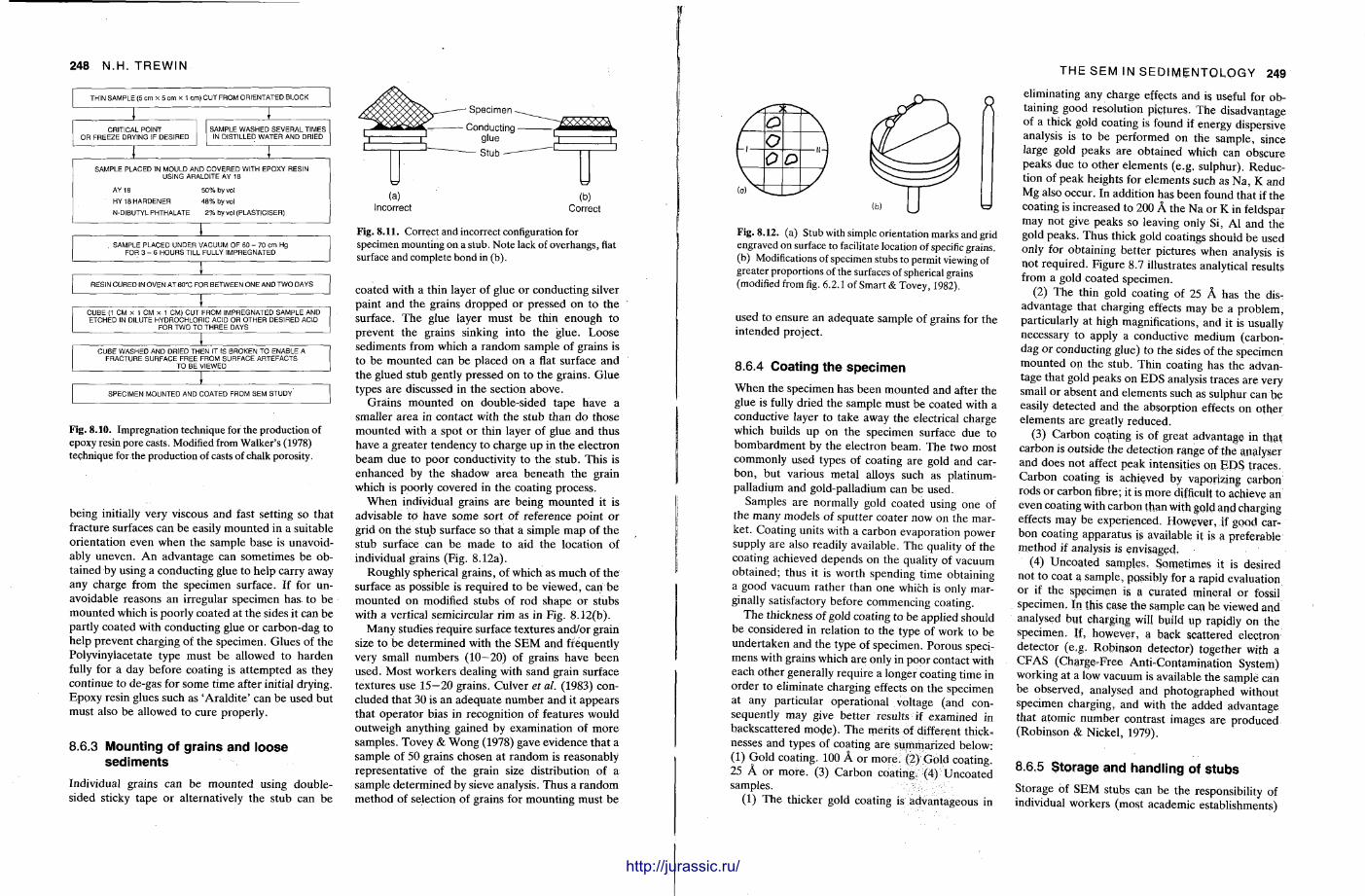
248 N.H. TREWIN
T H I N S A M P L E (5 c m x 5 c m x 1 c m ) C U T F R O M O R I E N T A T E D B L O C K
1 1 C R I T I C A L P O I N T
O R F R E E Z E D R Y I N G IF D E S I R E D S A M P L E W A S H E D S E V E R A L T I M E S
IN D I S T I L L E D W A T E R A N D D R I E D
J I S A M P L E P L A C E D IN M O U L D A N D C O V E R E D W I T H E P O X Y R E S I N
U S I N G A R A L D I T E A Y 18
A Y 18 5 0 % b y vol
H Y 1 8 H A R D E N E R 4 8 % by vol
N - D I B U T Y L P H T H A L A T E 2 % by vol ( P L A S T I C I S E R )
Z E Z ~ S A M P L E P L A C E D U N D E R V A C U U M O F 60 - 7 0 c m H g
F O R 3 - 6 H O U R S T I L L F U L L Y I M P R E G N A T E D
J ~ z z R E S I N C U R E D IN O V E N A T 80"C F O R B E T W E E N O N E A N D T W O D A Y S
z z z j ^ ^ ^ ^ z C U B E (1 C M X 1 C M x 1 C M ) C U T F R O M I M P R E G N A T E D S A M P L E A N D E T C H E D IN D I L U T E H Y D R O C H L O R I C A C I D O R O T H E R D E S I R E D A C I D
F O R T W O T O T H R E E D A Y S
. I Z Z C U B E W A S H E D A N D D R I E D T H E N IT IS B R O K E N T O E N A B L E A
F R A C T U R E S U R F A C E F R E E F R O M S U R F A C E A R T E F A C T S T O B E V I E W E D
~ T ~ S P E C I M E N M O U N T E D A N D C O A T E D F R O M S E M S T U D Y
Fig. 8.10. Impregnation technique for the production of epoxy resin pore casts. Modified from Walker's (1978) technique for the production of casts of chalk porosity.
being initially very viscous and fast setting so that fracture surfaces can be easily mounted in a suitable orientat ion even when t he sample base is unavoidably uneven. A n advantage can sometimes be obtained by using a conducting glue to help carry away any charge from the specimen surface. If for unavoidable reasons an irregular specimen has to be mounted which is poorly coated at the sides it can be partly coated with conducting glue or carbon-dag to help prevent charging of the specimen. Glues of the Polyvinylacetate type must be allowed to harden fully for a day before coating is a t tempted as they continue to de-gas for some time after initial drying. Epoxy resin glues such as 'Ara ld i te ' can be used bu t must also be allowed to cure properly.
8.6.3 Mounting of grains and loose sediments
Individual grains can be mounted using double-sided sticky tape or alternatively the stub can be
(a) (b) Incorrect Correct
Fig. 8.11. Correct and incorrect configuration for specimen mounting on a stub. Note lack of overhangs, flat surface and complete bond in (b).
coated with a thin layer of glue or conducting silver paint and the grains d ropped or pressed on to the surface. The glue layer must be thin enough to prevent the grains sinking into the glue. Loose sediments from which a random sample of grains is to be mounted can be placed on a flat surface and the glued stub gently pressed on to the grains. Glue types are discussed in the section above .
Grains mounted on double-sided t ape have a smaller area in contact with the stub than do those mounted with a spot or thin layer of glue and thus have a greater tendency to charge up in the electron beam due to poor conductivity to the s tub. This is enhanced by the shadow area benea th the grain which is poorly covered in the coating process.
When individual grains are being moun ted it is advisable to have some sort of reference point or grid on the stub surface so that a simple m a p of the stub surface can be made to aid the location of individual grains (Fig. 8.12a).
Roughly spherical grains, of which as much of the surface as possible is required to be viewed, can be mounted on modified stubs of rod shape or stubs with a vertical semicircular rim as in Fig. 8.12(b).
Many studies require surface textures and/or grain size to be determined with the S E M and frequently very small numbers (10—20) of grains have been used. Most workers dealing with sand grain surface textures use 15—20 grains. Culver et al. (1983) concluded that 30 is an adequate number and it appears that opera tor bias in recognition of features would outweigh anything gained by examination of more samples. Tovey & Wong (1978) gave evidence that a sample of 50 grains chosen at r andom is reasonably representat ive of the grain size distribution of a sample de termined by sieve analysis. Thus a r andom method of selection of grains for mount ing must be
THE SEM IN SEDIMENTOLOGY 249
1—5
o 1 o
O o II —
(a) Vl
Fig. 8.12. (a) Stub with simple orientation marks and grid engraved on surface to facilitate location of specific grains, (b) Modifications of specimen stubs to permit viewing of greater proportions of the surfaces of spherical grains (modified from fig. 6.2.1 of Smart & Tovey, 1982).
used to ensure an adequate sample of grains for the intended project.
8.6.4 Coating the specimen
When the specimen has been mounted and after the glue is fully dried the sample must be coated with a conductive layer to take away the electrical charge which builds u p on the specimen surface due t o bombardment by the electron beam. The two most commonly used types of coating are gold and carbon, but various metal alloys such as platinum-palladium and gold-palladium can be used.
Samples are normally gold coated using one of the many models of sputter coater now on the market . Coat ing units with a carbon evaporation power supply are also readily available. The quality of the coating achieved depends on the quality of vacuum obtained; thus it is worth spending time obtaining a good vacuum rather than one which is only marginally satisfactory before commencing coating.
The thickness of gold coating to be applied should be considered in relation to the type of work to be under taken and the type of specimen. Porous specimens with grains which are only in poor contact with each other generally require a longer coating t ime in order to eliminate charging effects on the specimen at any particular operat ional voltage (and consequently may give bet ter results if examined in backscattered mode) . The merits of different thicks nesses and types of coating are summarized below: (1) Gold coating. 100 A or more . (2) Gold coating. 25 A or m o r e . (3) Carbon coating. (4) Uncoa ted samples.
(1) T h e thicker gold coating is advantageous in
eliminating any charge effects and is useful for ob taining good resolution pictures. The disadvantage of a thick gold coating is found if energy dispersive analysis is to be performed on the sample, since large gold peaks are obtained which can obscure peaks due to other e lements (e.g. sulphur). Reduction of peak heights for elements such as Na, K and Mg also occur. In addition has been found that if the coating is increased to 200 A the Na or K in feldspar may not give peaks so leaving only Si, Al and the gold peaks . Thus thick gold coatings should be used only for obtaining bet ter pictures when analysis is not required. Figure 8.7 illustrates analytical results from a gold coated specimen.
(2) T h e thin gold coating of 25 A has t he disadvantage that charging effects may be a problem, particularly at high magnifications, and it is usually necessary to apply a conductive medium (carbon-dag or conducting glue) to the sides of the specimen moun ted on t he stub. Thin coating has the advantage that gold peaks on E D S analysis traces are very small or absent and elements such as sulphur can be easily detected and the absorpt ion effects on other elements are greatly reduced.
(3) Carbon coating is of great advantage in that carbon is outside the detect ion range of the analyser and does not affect peak intensities on E D S traces. Carbon coating is achieved by vaporizing carbon rods or carbon fibre; it is more difficult to achieve an even coating with carbon than with gold and charging effects may be experienced. However , if good carbon coating apparatus is available it is a preferable method if analysis is envisaged,
(4) Uncoa ted samples. Sometimes it is desired not to coat a sample, possibly for a rapid evaluation or if the specimen is a eurated mineral or fossil specimen, In this ease the sample can be viewed and analysed but charging will build up rapidly on the specimen. If, however, a back scattered electron detector (e,g. Robinson detector) together with a C F A S (Charge-Free Anti -Contaminat ion System) working at a low vacuum is available the sample can be observed, analysed and photographed without specimen charging, and with the added advantage that atomic number contrast images are produced (Robinson & Nickel, 1979).
8.6.5 Storage and handling of stubs
Storage of SEM stubs can be the responsibility of individual workers (most academic establishments)
http://jurassic.ru/
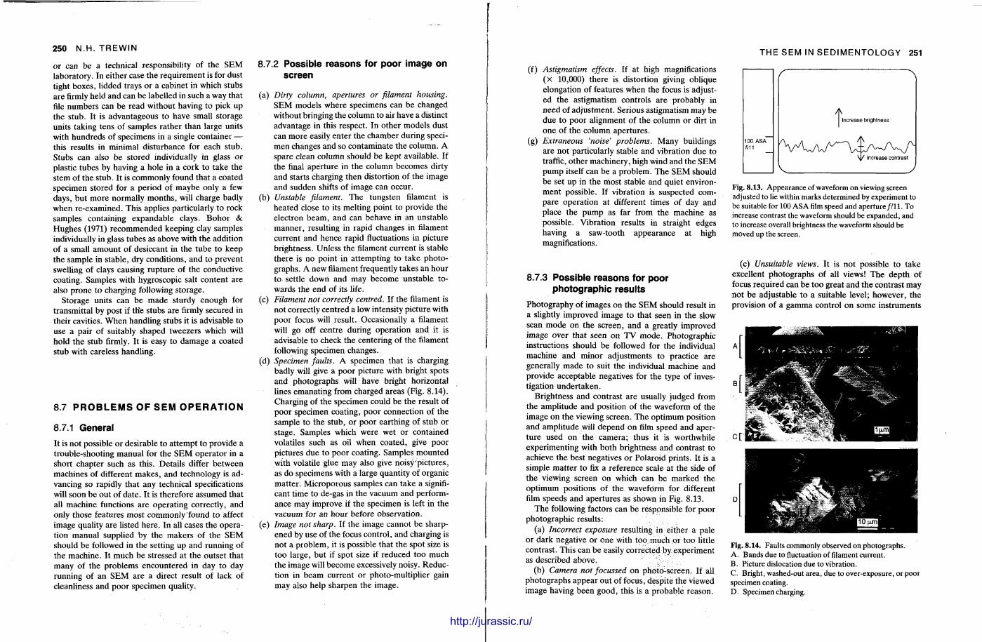
250 N.H. TREWIN
or can be a technical responsibility of the SEM laboratory. In either case the requirement is for dust tight boxes, lidded trays or a cabinet in which stubs are firmly held and can be labelled in such a way that file numbers can be read without having to pick up the stub. It is advantageous to have small storage units taking tens of samples ra ther than large units with hundreds of specimens in a single container — this results in minimal disturbance for each stub. Stubs can also be stored individually in glass or plastic tubes by having a hole in a cork to take the stem of the stub. It is commonly found that a coated specimen stored for a period of maybe only a few days, but more normally months , will charge badly when re-examined. This applies particularly to rock samples containing expandable clays. Bohor & Hughes (1971) recommended keeping clay samples individually in glass tubes as above with the addition of a small amount of desiccant in the tube to keep the sample in stable, dry conditions, and to prevent swelling of clays causing rupture of the conductive coating. Samples with hygroscopic salt content are also prone to charging following storage.
Storage units can be m a d e sturdy enough for transmittal by post if ttie stubs are firmly secured in their cavities. When handling stubs it is advisable to use a pair of suitably shaped tweezers which will hold the stub firmly. It is easy to damage a coated stub with careless handling.
8.7 P R O B L E M S OF S E M O P E R A T I O N
8.7.1 General
It is not possible or desirable to a t tempt to provide a trouble-shooting manual for the S E M opera tor in a short chapter such as this. Details differ between machines of different makes , and technology is advancing so rapidly that any technical specifications will soon be out of da te . It is therefore assumed that all machine functions are operat ing correctly, and only those features most commonly found to affect image quality are listed here . In all cases the operation manual supplied by the makers of the S E M should be followed in the setting up and running of the machine. It much be stressed at the outset that many of the problems encountered in day to day running of an S E M are a direct result of lack of cleanliness and poor specimen quality.
8.7.2 Possible reasons for poor image on screen
(a) Dirty column, apertures or filament housing. S E M models where specimens can be changed without bringing the column to air have a distinct advantage in this respect. In other models dust can more easily enter the chamber during specimen changes and so contaminate the column. A spare clean column should be kept available. If the final aper ture in the column becomes dirty and starts charging then distortion of the image and sudden shifts of image can occur.
(b) Unstable filament. The tungsten filament is heated close to its melting point to provide the electron beam, and can behave in an unstable manner , resulting in rapid changes in filament current and hence rapid fluctuations in picture brightness. Unless the filament current is stable there is no point in at tempting to t ake photographs. A new filament frequently takes an hour to settle down and may become unstable towards the end of its life.
(c) Filament not correctly centred. If the filament is not correctly centred a low intensity picture with poor focus will result. Occasionally a filament will go off centre during operat ion and it is advisable to check the centering of the filament following specimen changes.
(d) Specimen faults. A specimen that is charging badly will give a poor picture with bright spots and photographs will have bright horizontal lines emanat ing from charged areas (Fig. 8.14). Charging of the specimen could be the result of poor specimen coating, poor connection of the sample t o the s tub, or poor earthing of stub or stage. Samples which were wet or contained volatiles such as oil when coated, give poor pictures due to poor coating. Samples mounted with volatile glue may also give noisy 'pictures, as do specimens with a large quantity of organic mat ter . Microporous samples can take a significant t ime to de-gas in the vacuum and performance may improve if the specimen is left in the vacuum for an hour before observation.
(e) Image not sharp. If the image cannot be sharpened by use of the focus control , and charging is not a problem, it is possible that the spot size is too large, but if spot size if reduced too much the image will become excessively noisy. Reduction in beam current or photo-multiplier gain may also help sharpen the image.
r
THE SEM IN SEDIMENTOLOGY 251
(f) Astigmatism effects. If at high magnifications ( x 10,000) there is distortion giving oblique elongation of features when the focus is adjusted the astigmatism controls are probably in need of adjustment. Serious astigmatism may be due to poor alignment of the column or dirt in one of the column aper tures .
(g) Extraneous 'noise' problems. Many buildings are not particularly stable and vibration due to traffic, o ther machinery, high wind and the SEM p u m p itself can be a problem. The S E M should be set up in the most stable and quiet environment possible. If vibration is suspected compare operat ion at different times of day and place the p u m p as far from the machine as possible. Vibrat ion results in straight edges having a saw-tooth appearance at high magnifications.
100 ASA ff11
Increase brightness
V Increase contrast
Fig. 8.13. Appearance of waveform on viewing screen adjusted to lie within marks determined by experiment to be suitable for 100 ASA film speed and aperture / / l 1. To increase contrast the waveform should be expanded, and to increase overall brightness the waveform should be moved up the screen.
8.7.3 Possible reasons for poor photographic results
Photography of images on the SEM should result in a slightly improved image to tha t seen in t he slow scan mode on the screen, and a greatly improved image over that seen on T V mode . Photographic instructions should be followed for the individual machine and minor adjustments to practice are generally made to suit the individual machine and provide acceptable negatives for the type of investigation under taken .
Brightness and contrast are usually judged from the ampli tude and position of the waveform of the image on the viewing screen. T h e opt imum position and ampli tude will depend on film speed and aperture used on the camera; thus it is worthwhile experimenting with both brightness and contrast to achieve the best negatives or Polaroid prints . It is a simple mat te r to fix a reference scale at the side of the viewing screen on which can be marked the opt imum positions of the waveform for different film speeds and apertures as shown in Fig. 8.13.
T h e following factors can be responsible for poor photographic results:
(a) Incorrect exposure resulting in either a pale or dark negative or one with too much or too little contrast . This can be easily corrected by experiment as described above.
(b) Camera not focussed on photo-screen- If all photographs appear out of focus, despite the Viewed image having been good, this is a probable reason.
(c) Unsuitable views. It is not possible to take excellent photographs of all views! The depth of focus required can be too great and the contrast may not be adjustable to a suitable level; however , the provision of a gamma control on some instruments
Fig. 8.14. Faults commonly observed on photographs. A. Bands due to fluctuation of filament current. B. Picture dislocation due to vibration. C. Bright, washed-out area, due to over-exposure, or poor specimen coating. D. Specimen charging.
http://jurassic.ru/
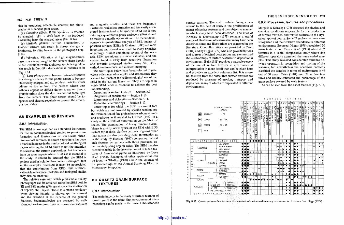
252 N .H . T R E W I N
aids in producing aeeeptabie contrast for photography in otherwise poof areas .
(d) Charging effects. if the specimen is affected by charging* light or dark fines will be produced emanat ing Itom the charged areas (Fig. 8.14).
(g) Unstable jilaWent current. Fluctuations in filament current wili result in abrupt changes in brightness; forming bands on the photograph (Fig.
8.14); (f) Vibration. Vibrat ion at high magnifications
results in a wavy image on the screen; sharp knocks to the instrument while a photograph is being taken can result in fault-like dislocations in pictures as in Fig. 8.14.
(g) Dirty photo-screen. In some instruments there is a s trong tendency for the photo-screen to become electrically charged and attract dust particles which adhere to the surface. T h e patches where dust adheres appear as diffuse darker areas on photographic prints since the dust has cut ou t some light from the camera. T h e photo-screen should b e inspected and cleaned regularly to prevent the accumulation of dust .
8.8 E X A M P L E S A N D R E V I E W S
8.8.1 i n t r o d u c t i o n
The SEM is now regarded as a standard instrument for use in sedimentological studies to provide information and illustrations of small-scale three-dimensional surfaces. In recent years there has been a marked increase in the number of sedimentological papers utilizing the S E M and it is not the intention to review all the current applications, but to concentra te on some aspects where S E M use is essential to the study. It should be stressed that the S E M is seldom used in isolation from other techniques; thus in the examples discussed it must be appreciated that the contribution f rom X R D , thin sections, cathodoluminescence, isotopes and biologieal studies may also be essential.
The relative ease with which publish&ble quality photographs can be obtained Using the S E M both in SE and B S E mode's gives great scope for illustration of reports and papers . There is a strong tendency when viewing Material to photograph the unusual and the beautiful at the expense of the general features. Sedimentologists are attracted by well-founded aeolian quartz grains, vermicular kaolinite
and aragonite needles , and these a re frequently illustrated, whilst less attractive and less easily interpreted features tend to be ignored. S E M use is now entering a quantitative phase and every effort should be made to quantify observations. T h e recent developments in quantitative analysis of B S E images of polished surfaces (Dilks & G r a h a m , 1985) are most important and should contribute to many branches of geology. Studies combining several of the available SEM techniques are most valuable, and the current trend is away from repetitive illustration and towards integrated studies using S E , BSE, cathodoluminescence and element mapping.
The four topics below have been selected to provide a wide range of examples and also because they account for much of the sedimentological use of the S E M in the current l i terature. They a re topics in which SEM work is essential to achieve the best understanding.
Quar tz grain surface textures — Section 8.9. Diagenesis of sandstones — Section 8.10. Limestones and dolomites —• Section 8.11. Endoli thic microborings — Section 8.12. O the r topics for which the S E M is a useful tool
but which a re not covered by specific sections a re the examination of fine grained non-carbonate muds and mudrocks as illustrated by O'Brien (1987) in a study on the effects of bioturbation on the fabric of shales. The examination of heavy mineral assemblages is greatly aided by use of the S E M with E D S system for analysis. Surface textures of grains other than quartz are also providing useful information as in the study by Hansley (1987) comparing natural etch features on garnets with those produced experimentally using organic acids. The SEM has also proved valuable in the investigation of detailed features of framboidal pyrite as illustrated by Love et al. (1984). Examples of other applications can be found in Whalley (1978) and in the volumes of the proceedings of the Annual Scanning Electron Microscopy Symposium.
8.9 Q U A R T Z G R A I N S U R F A C E T E X T U R E S
8.9.1 Introduction The main impetus in the study of surface textures of quartz grains is the belief that environmental interpretat ions can be made on the basis of characteristic
THE SEM IN SEDIMENTOLOGY 253
surface textures. T h e main problem facing a new recruit to this field of study is the proliferation of names of surface features and the subjective manner in which many have been described. The atlas of Krinsley & D o o r n k a m p (1973) remains a useful source of illustration of textures but many have been described since and illustrations are scattered in the l i terature. G o o d illustrations are provided by Cater (1984) and by Higgs (1979) who also gave definitions and sources of original descriptions and summarized the relationships of surface textures to depositional environment . Bull (1981) provides a valuable review of the use of surface textures in environmental interpretat ion in more detail than can be given here and provides an excellent reference list. It is essential to stress from the outset that surface textures are produced by processes of erosion, t ransport and deposit ion, many of which are duplicated in different environments .
8.9.2 Processes, textures and procedures
Margolis & Krinsley (1974) discussed the physical and chemical conditions responsible for the production of surface textures , and related textures to the crystallography of quartz . Some 22 surface textures were recognized and their relative abundance in different environments discussed. Higgs (1979) recognized 30 main textures and Culver et al. (1983) utilized 32 features in a useful comparat ive study where five different operators examined the same coded samples. This study revealed considerable variance between operators in recognition and scoring of the textures , but nevertheless the operators correctly classified the samples in terms of environment in 49 out of 50 cases. Cater (1984) used 22 surface textures and usually est imated the percentage of the grain surface covered by each feature.
As can be seen from the list of features (Fig. 8.15,
S U R F A C E F E A T U R E
ex.
% GRAINS SHOWING FEATURE
[»] ABUNDANT >75
[•] COMMON 25 - 75
[ o ] SPARSE 25 - 75
RARE < 5
I 1 SMALL IRREGULAR PITS (<10M)
| 2 MEDIUM IRREGULAR PITS | 3 LARGE IRREGULAR PITS (>100p) | 4 SMALL C0NCH0IDAL FRACTURE (<10fi) | 5 MEDIUM C0NCH0IDAL FRACTURE | 6 LARGE CONCHO I DAL FRACTURE (>1 OOf.) | 7 STRAIGHT STEPS
'.J I 8 ARCUATE STEPS | 9 FRACTURE PLATES/PLANES | 10 PARALLEL STRIATIONS | 11 IMBRICATED
GRINDING FEATURES | 12 ADHERING PARTICLES | 13 MEANDERING RIDGES | 14 STRAIGHT SCRATCHES | 15 CURVED SCRATCHES | 16 V
's | 17 ANGULAR OUTLINE | 18 ROUNDED OUTLINE | 19
LOW RELIEF (<0.5jj) | 20 MEDIUM RELIEF | 21 HIGH RELIEF
(>10p) | 22 ORIENTED ETCH PITS | 23 ANASTOMOSING ETCH PATTERN | 24 SOLUTION PITS | 25 SOLUTION CREVASSES | 26
SCALING | 27 SILICA GLOBULES I 28 SILICA FLOWERS | 29 SILICA PELLICLE | 30 CRYSTALLINE OVERGROWTH
C R Y S T A L I N E SOURCE ROCK • • • • • • • • • •
SU
BA
QU
EO
US
|
r LOW ENERGY r . „ , l r 1 MEDIUM ENERGY FLUVIAT1LE HIGH ENERGY
I TORRENTIAL
o O o • • • • • o
SU
BA
QU
EO
US
|
r LOW ENERGY r . „ , l r 1 MEDIUM ENERGY FLUVIAT1LE HIGH ENERGY
I TORRENTIAL
o o o • • • • •
SU
BA
QU
EO
US
|
r LOW ENERGY r . „ , l r 1 MEDIUM ENERGY FLUVIAT1LE HIGH ENERGY
I TORRENTIAL •
SU
BA
QU
EO
US
|
r LOW ENERGY r . „ , l r 1 MEDIUM ENERGY FLUVIAT1LE HIGH ENERGY
I TORRENTIAL • • • • • •
SU
BA
QU
EO
US
|
DELTAIC •
r SUBAERIAL MARSH
( LANDWARD CHANNEL < MEDIAL
I SEAWARD
o o o • • • • •
SU
BA
QU
EO
US
|
DELTAIC •
r SUBAERIAL MARSH
( LANDWARD CHANNEL < MEDIAL
I SEAWARD
o o o • • • o
SU
BA
QU
EO
US
|
DELTAIC •
r SUBAERIAL MARSH
( LANDWARD CHANNEL < MEDIAL
I SEAWARD
o o o • • • • O •
SU
BA
QU
EO
US
|
DELTAIC •
r SUBAERIAL MARSH
( LANDWARD CHANNEL < MEDIAL
I SEAWARD o o o • • • o o
SU
BA
QU
EO
US
|
DELTAIC •
r SUBAERIAL MARSH
( LANDWARD CHANNEL < MEDIAL
I SEAWARD • • O
SU
BA
QU
EO
US
|
MARINE / INTERTIDAL " A K 1 N t \ SUBTIDAL • o o O o • • • o • O • O o S
UB
AQ
UE
OU
S |
MARINE / INTERTIDAL " A K 1 N t \ SUBTIDAL • • • • o • • • 0
' COASTAL AEOLIAN <y HOT DESERT ' • o o o o o o • o • ' COASTAL AEOLIAN <y HOT DESERT ' • o o • o o • • o o O O
GLACIAL • • • • • • • • • o • • • • • f SILICA ••. / TEMPERATE : • • • • o o
PED0L0GIC J DISSOLVED '.\ TROPICAL • • • • • • • • PED0L0GIC | SILICA '/'TEMPERATE.';' • • • • o • • I PRECIPITATED \ IRC'ICAI • • • • • • •
SUBSURFACE D I A G E N £;T .J-.C : • • • • • • • • • • Fig. 8.15. Quartz grain surface textures characteristic of various sedimentary environments. Redrawn from Higgs (1979).
http://jurassic.ru/
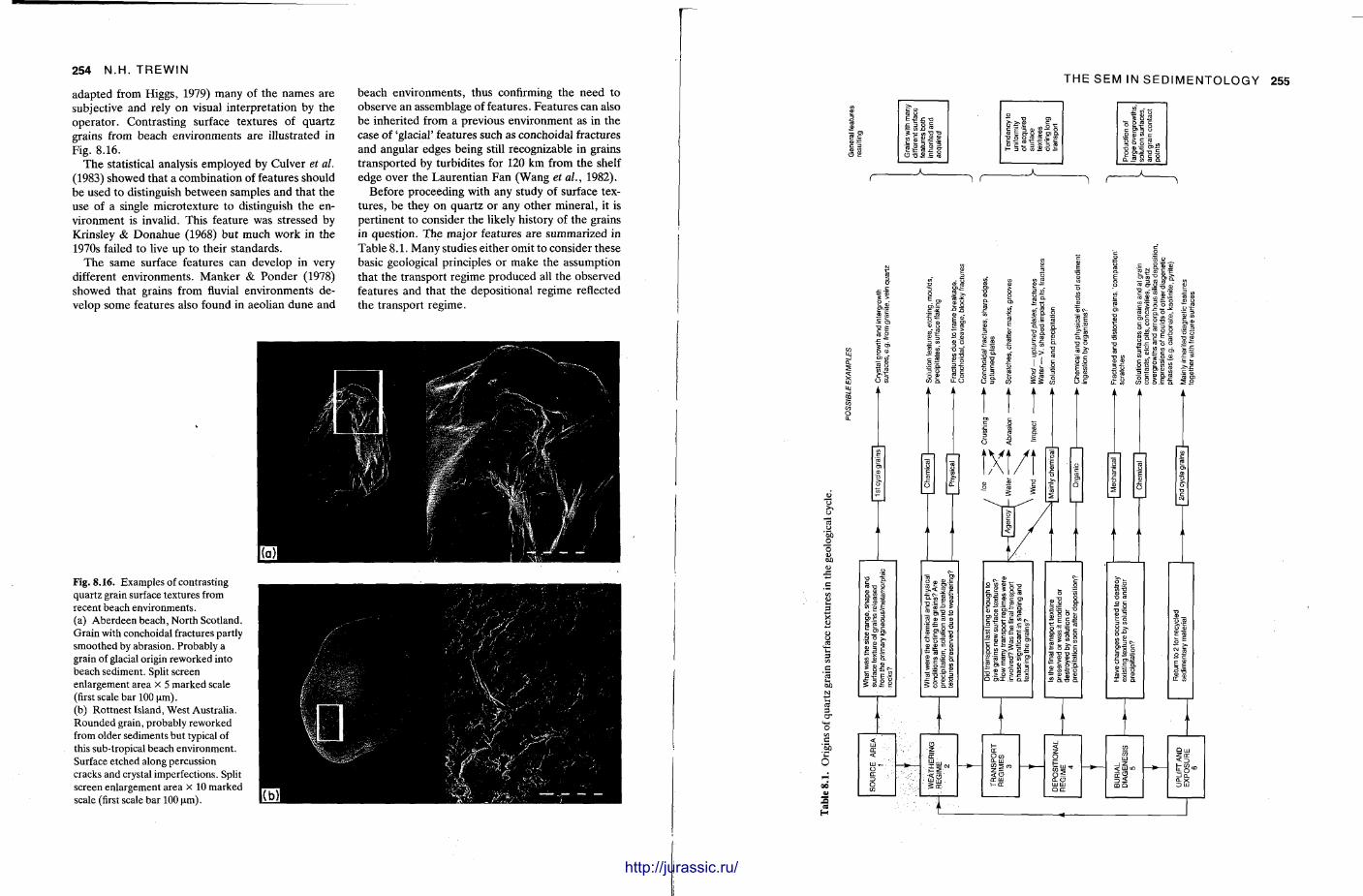
254 N.H. TREWIN
beach envi ronments , thus confirming the need to observe an assemblage of features. Fea tures can also be inheri ted from a previous environment as in the case of 'glacial' features such as conchoidal fractures and angular edges being still recognizable in grains t ransported by turbidites for 120 km from the shelf edge over the Laurent ian Fan (Wang et al., 1982).
Before proceeding with any study of surface textures , be they on quartz or any other mineral , it is pert inent to consider the likely history of the grains in quest ion. The major features are summarized in Table 8 .1 . Many studies either omit to consider these basic geological principles or make the assumption that the t ransport regime produced all the observed features and that the depositional regime reflected the transport regime.
Fig. 8.16. Examples of contrasting quartz grain surface textures from recent beach environments. (a) Aberdeen beach, North Scotland. Grain with conchoidal fractures partly smoothed by abrasion. Probably a grain of glacial origin reworked into beach sediment. Split screen enlargement area x 5 marked scale (first scale bar 100 u m ) . (b) Rottnest Island, West Australia. Rounded grain, probably reworked from older sediments but typical of this sub-tropical beach environment. Surface etched along percussion cracks and crystal imperfections. Split screen enlargement area x 10 marked scale (first scale bar 100 urn).
1 >
d . > - t ^
60 O
3
c ' 5b
1 E
5 S
») j) E
Si. « =3
£ £ " — X c « O Q.
S S i c
f i l l !
THE SEM IN SEDIMENTOLOGY 255
wth
s,
ces,
ta
ct C CD
CO cj E S r n
O ~ T3 CD
wth
s,
ces,
ta
ct
resu
ltin
g
Gra
ins
wit
h i
d
iffer
ent
sur
feat
ure
s bo
tl in
her
ited
am
ac
quired
Ten
den
cy
un
ifo
rmit
y of
acq
uir
e
surf
ace
text
ure
s d
uri
ng
Ion
tr
ansp
ort
Pro
du
ctio
n o
f la
rge
ove
rgro
so
luti
on
su
rfa
and
gra
in c
on
p
oin
ts
r
s i 3 CO
o £ W CL
en 2 2 >•
e s,
CO "D £ ' 5 3 -C
O-
cal
mg
hys
i ?
An O)
hys
i ?
An
ika . c
Q. to •o c
cd C '(0 3 CO •o o CO
CO CO .9 jc 3
hem
in
gt
utio
r e
dd
" o CO o so
l
^ te to — CO CO o
Q_
twe
itior
p
ita
res
ro ~o 3
5 8 Q.
-zz
y LL
; LULU •
Cl"0
CO £ • E ™ 3 CO
Co
1 1
CO c
t l "D. O) -o o
E w CO <D
0l LI!
<o r r m r- rr
c o g *
a. <D Ud UJ q rr
,E R • £ co « m c
•K 3 TO CO g coco 9? O] -— 3
O CD
s = ,_ > o o n
'ro S "S . o "f-
CO JZ ™ O "
i f f I t
. J i l l — c © a c
,9 O > C X
. 9 1 io
a o. TO 5 . i S
5 | ™ ro S E § 1
< HI in
I S m O
adapted from Higgs, 1979) many of the names are subjective and rely on visual interpretat ion by the opera tor . Contrast ing surface textures of quar tz grains from beach environments are illustrated in Fig. 8.16.
T h e statistical analysis employed by Culver et al. (1983) showed that a combinat ion of features should be used to distinguish between samples and that the use of a single microtexture to distinguish the environment is invalid. This feature was stressed by Krinsley & D o n a h u e (1968) but much work in the 1970s failed to live up to their s tandards .
T h e same surface features can develop in very different environments . M a n k e r & Ponder (1978) showed that grains from fluvial environments develop some features also found in aeolian dune and
http://jurassic.ru/
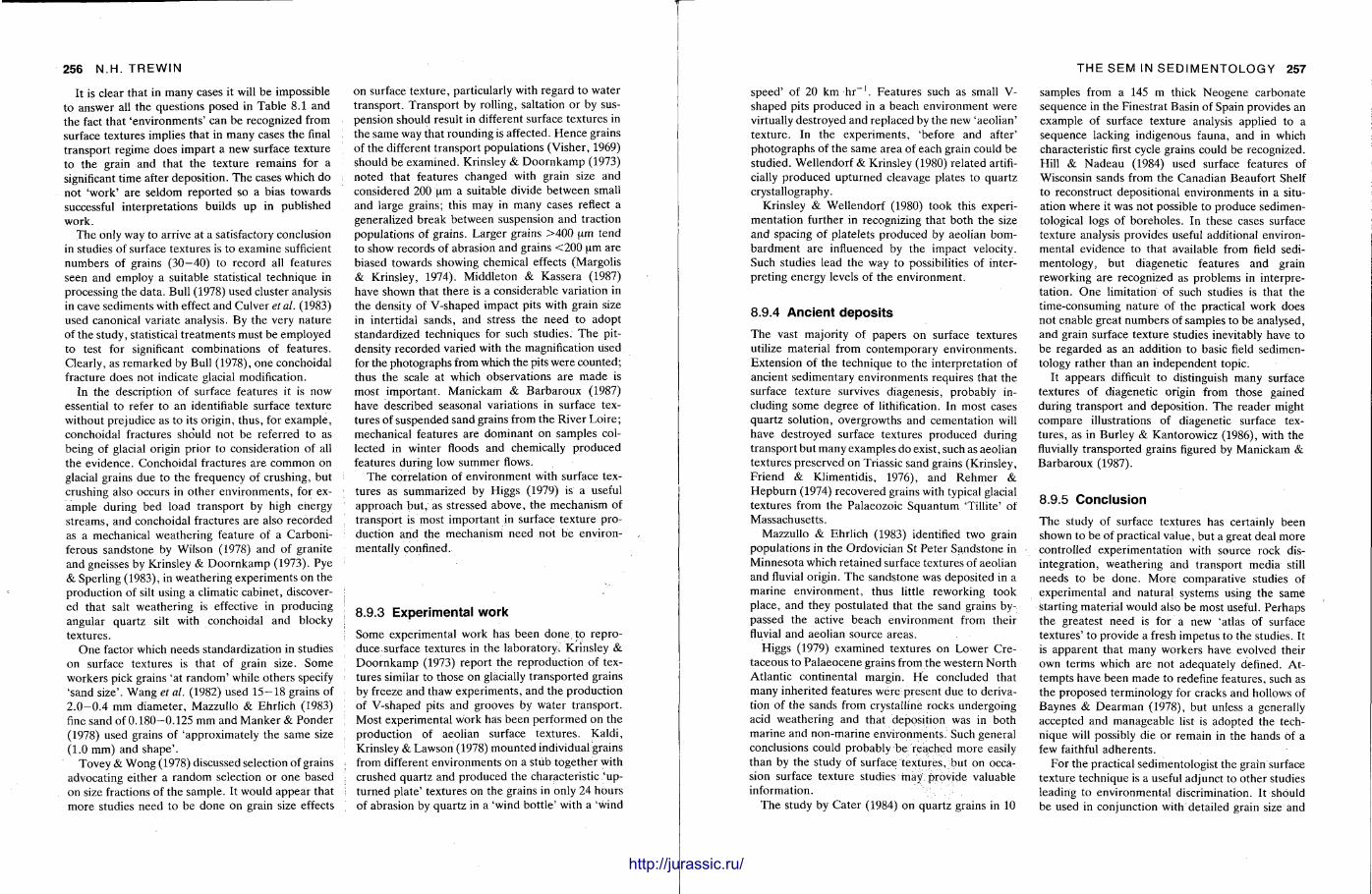
256 N.H. TREWIN
It is clear that in many cases it will be impossible to answer all the questions posed in Table 8.1 and the fact that ' environments ' can be recognized from surface textures implies that in many cases the final t ransport regime does impart a new surface texture to the grain and that the texture remains for a significant t ime after deposit ion. The cases which do not 'work ' are seldom repor ted so a bias towards successful interpretat ions builds up in published work.
The only way to arrive at a satisfactory conclusion in studies of surface textures is to examine sufficient numbers of grains ( 3 0 - 4 0 ) to record all features seen and employ a suitable statistical technique in processing the data . Bull (1978) used cluster analysis in cave sediments with effect and Culver etal. (1983) used canonical variate analysis. By the very nature of the study, statistical t rea tments must be employed to test for significant combinations of features. Clearly, as remarked by Bull (1978), one conchoidal fracture does not indicate glacial modification.
In the description of surface features it is now essential to refer to an identifiable surface texture without prejudice as to its origin, thus, for example , conchoidal fractures should not be referred to as being of glacial origin prior to considerat ion of all the evidence. Conchoidal fractures are common on glacial grains due to the frequency of crushing, but crushing also occurs in o ther environments , for example during bed load transport by high energy s t reams, and conchoidal fractures are also recorded as a mechanical weathering feature of a Carboniferous sandstone by Wilson (1978) and of granite and gneisses by Krinsley & D o o r n k a m p (1973). Pye & Sperling (1983), in weathering experiments on the product ion of silt using a climatic cabinet , discovered that salt weathering is effective in producing angular quartz silt with conchoidal and blocky textures.
One factor which needs standardization in studies on surface textures is that of grain size. Some workers pick grains 'at r andom' while o thers specify 'sand size'. Wang et al. (1982) used 1 5 - 1 8 grains of 2 . 0 - 0 . 4 m m diameter , Mazzullo & Ehrlich (1983) fine sand of 0.180—0.125 mm and Manker & Ponder (1978) used grains of 'approximately the same size (1.0 mm) and shape ' .
Tovey & Wong (1978) discussed selection of grains advocating either a random selection or one based on size fractions of the sample. It would appear that more studies need to be done on grain size effects
on surface texture , particularly with regard to water t ransport . Transpor t by rolling, saltation or by suspension should result in different surface textures in the same way that rounding is affected. Hence grains of the different t ransport populat ions (Visher, 1969) should be examined. Krinsley & D o o r n k a m p (1973) noted that features changed with grain size and considered 200 um a suitable divide between small and large grains; this may in many cases reflect a generalized break between suspension and traction populat ions of grains. Larger grains > 4 0 0 um tend to show records of abrasion and grains < 2 0 0 urn are biased towards showing chemical effects (Margolis & Krinsley, 1974). Middleton & Kassera (1987) have shown that there is a considerable variation in the density of V-shaped impact pits with grain size in intertidal sands, and stress the need to adopt standardized techniques for such studies. T h e pit-density recorded varied with the magnification Used for the photographs from which the pits were counted; thus the scale at which observations are m a d e is most important . Manickam & Barbaroux (1987) have described seasonal variations in surface textures of suspended sand grains from the River Loire; mechanical features are dominant on samples collected in winter floods and chemically produced features during low summer flows.
The correlation of environment with surface textures as summarized by Higgs (1979) is a useful approach but , as stressed above, the mechanism of t ransport is most important in surface texture production and the mechanism need not be environmentally confined.
8.9.3 Experimental work
Some experimental work has been done to reproduce surface textures in the laboratory. Krinsley & D o o r n k a m p (1973) report the reproduct ion of textures similar to those on glacially t ransported grains by freeze and thaw exper iments , and the production of V-shaped pits and grooves by water t ransport . Most experimental work has been performed on the production of aeolian surface textures. Kaldi , Krinsley & Lawson (1978) mounted individual grains from different environments on a stub together with crushed quartz and produced the characteristic 'upturned pla te ' textures on the grains in only 24 hours of abrasion by quar tz in a 'wind bott le ' with a 'wind
THE SEM IN SEDIMENTOLOGY 257
speed ' of 20 km - h r - 1 . Features such as small V-shaped pits produced in a beach environment were virtually destroyed and replaced by the new 'aeolian ' texture . In the exper iments , 'before and after' photographs of the same area of each grain could be studied. Wellendorf & Krinsley (1980) related artificially produced upturned cleavage plates to quartz crystallography.
Krinsley & Wellendorf (1980) took this experimentat ion further in recognizing that both the size and spacing of platelets produced by aeolian bombardment are influenced by the impact velocity. Such studies lead the way to possibilities of interpreting energy levels of the environment .
8.9.4 Ancient deposits
The vast majority of papers on surface textures utilize material from contemporary environments . Extension of the technique to the interpretat ion of ancient sedimentary environments requires that the surface texture survives diagenesis, probably including some d e g T e e of lithification. In most cases quartz solution, overgrowths and cementat ion will have destroyed surface textures produced during t ransport but many examples do exist, such as aeolian textures preserved on Triassic sand grains (Krinsley, Friend & Klimentidis, 1976), and Rehmer & H e p b u r n (1974) recovered grains with typical glacial textures from the Palaeozoic Squantum 'Tillite' of Massachusetts .
Mazzullo & Ehrlich (1983) identified two grain populat ions in the Ordovician St Peter Sandstone in Minnesota which retained surface textures of aeolian and fluvial origin. T h e sandstone was deposi ted in a marine environment , thus little reworking took place, and they postulated that the sand grains bypassed the active beach environment from their fluvial and aeolian source areas .
Higgs (1979) examined textures on Lower Cretaceous to Palaeocene grains from the western Nor th Atlant ic continental margin. He concluded that many inherited features were present due to derivation of the sands from crystalline rocks undergoing acid weathering and that deposition was in both marine and non-marine environments . Such general conclusions could probably b e reached more easily than by the study of surface tex tures , but on occasion surface texture studies may: provide valuable information.
The study by Cater (1984) on quartz grains in 10
samples from a 145 m thick Neogene carbonate sequence in the Finestrat Basin of Spain provides an example of surface texture analysis applied to a sequence lacking indigenous fauna, and in which characteristic first cycle grains could be recognized. Hill & Nadeau (1984) used surface features of Wisconsin sands from the Canadian Beaufort Shelf to reconstruct depositional environments in a situation where it was not possible to produce sedimentological logs of boreholes . In these cases surface texture analysis provides Useful additional environmental evidence to that available from field sedimentology, but diagenetic features and grain reworking are recognized as problems in interpretation. O n e limitation of such studies is that the t ime-consuming nature of the practical work does not enable great numbers of samples to be analysed, and grain surface texture studies inevitably have to be regarded as an addition to basic field sedimentology rather than an independent topic.
It appears difficult to distinguish many surface textures of diagenetic origin from those gained during t ransport and deposit ion. The reader might compare illustrations of diagenetic surface textures , as in Burley & Kantorowicz (1986), with the fluvially t ransported grains figured by Manickam & Barbaroux (1987).
8.9.5 Conclusion
T h e study of surface textures has certainly been shown to be of practical value, but a great deal more controlled experimentat ion with source rock disintegration, weathering and transport media still needs to be done . More comparat ive studies of experimental and natural systems using the same starting material would also be most useful. Perhaps the greatest need is for a new 'atlas of surface textures ' to provide a fresh impetus to the studies. It is apparent that many workers have evolved their own terms which are not adequately defined. Attempts have been made to redefine features, such as the proposed terminology for cracks and hollows of Baynes & Dea rman (1978), but unless a generally accepted and manageable list is adopted the technique will possibly die or remain in the hands of a few faithful adherents .
For the practical sedimentologist the grain surface texture technique is a useful adjunct to other studies leading to environmental discrimination. It should be used in conjunction with detailed grain size and
http://jurassic.ru/
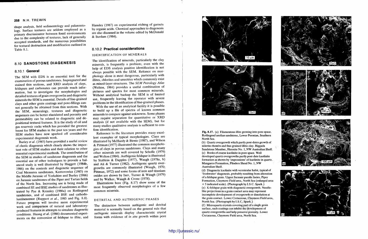
258 N.H. TREWIN
shape analysis, field sedimentology and pa laeontology. Surface textures are seldom employed as a primary discriminator between fossil environments due to the complexity of textures , lack of generally accepted s tandards , and the numerous possibilities for textural destruction and modification outl ined in Table 8 .1 .
8.10 S A N D S T O N E D I A G E N E S I S
8.10.1 General The SEM with E D S is an essential tool for the examination of porous sandstones. Impregnated and stained thin sections, and X R D analysis of clays, feldspars and carbonates can provide much information, but to investigate the morphologies and detailed textures of grain overgrowths and diagenetic minerals the S E M is essential. Details of fine-grained clays and o ther grain coatings and pore-fillings cannot generally be obtained from thin sections. With the S E M , mineralogy, textures and diagenetic sequences can be bet ter elucidated and porosity and permeabil i ty can be related to diagenetic and depositional textural features. It is the study of oil and gas reservoir rocks which has provided the greatest boost for S E M studies in the past ten years and the SEM studies have now sparked off considerable experimental diagenesis work.
Burley et al. (1985) have provided a useful review of clastic diagenesis which clearly shows the important role of SEM studies and their relation to other essential experimental methods . The contribution of the S E M in studies of sandstone diagenesis and the essential use of o the r techniques to provide a balanced study is well illustrated by Hugget t (1984b, 1986) on the controls and diagenetic sequence of Coal Measures sandstones, Kantorowicz (1985) on the Middle Jurassic of Yorkshi re and Burley (1986) on Jurassic sandstones of the Piper and Tar tan fields of the Nor th Sea. Increasing use is being made of combined SE and B S E studies of sandstones as illust ra ted by Pye & Krinsley (1986a) on Rotl iegend sandstones, and of combined B S E and cathodoluminescence (Rupper t et al., 1985 and Fig. 8.8). Future progress will involve more exper imental work and comparison of natural and laboratory-produced features in a t tempts to simulate diagenetic conditions. Huang et al. (1986) documented experiments on the conversion of feldspar to illite, and
Hansley (1987) on experimental etching of garnets by organic acids. Chemical approaches to diagenesis are also discussed in the volume edited by McDonald & Surdam (1984).
8.10.2 Practical considerat ions
I D E N T I F I C A T I O N O F M I N E R A L S
T h e identification of minerals , particularly the clay minerals , is frequently a p rob lem; even with the help of E D S analysis positive identification is not always possible with the S E M . Reliance on morphology alone is most dangerous , particularly with illites, chlorites and smectites which commonly exist as mixed-layer structures. T h e SEM Petrology Atlas (Wel ton, 1984) provides a useful combinat ion of pictures and spectra for most common minerals. Without analytical backup the S E M is of limited use, frequently leaving the opera to r with severe problems in the identification of fine-grained phases.
With the use of an analytical facility it is possible to build up a file of spectra of known common minerals to compare against unknowns . Some phases may require separation for quanti tat ive or X R D analysis (if not available with the S E M ) , but for many studies qualitative analysis is sufficient to confirm identification.
Reference to the l i terature provides many excellent examples of typical morphologies . Clays are illustrated by McHardy & Birnie (1987), and Wilson & Pi t tman (1977) illustrated the common morphologies of clays in porous sandstones. Clays and many other minerals are well covered by Scholle (1979) and Wel ton (1984). Authigenic feldspar is illustrated by Stablein & Dapp les (1977), Waugh (1978a, b ) and Ali & Turner (1982). Authigenic quartz overgrowths are commonly illustrated (Waugh , 1970; Pi t tman, 1972) and some forms of iron and ti tanium oxides are shown by Ixer, Turne r & Waugh (1979) and by Walker , Waugh & Crone (1978).
Illustrations he re (Fig. 8.17) show some of the most frequently observed morphologies of a few common minerals .
D E T R I T A L A N D A U T H I G E N I C P H A S E S
T h e distinction between authigenic and detrital material is normally based on the general rule that authigenic minerals display characteristic crystal forms with evidence of in situ growth within pore
Fig. 8.17. (a) Filamentous illite growing into pore space. Rotliegend aeolian sandstone, Lower Permian, Southern North Sea. (b) Quartz overgrowth which partly post-dates growth of siderite rhombs and fine-grained illitic clay. Biggada Sandstone Member, Hermite No. 1, NW Australian Shelf. (c) Books of coarse kaolinite in pore space. Well developed quartz overgrowths partly post-date kaolinite formation as shown by 'impressions' of kaolinite in quartz. Mungaroo Formation, Flinders Shoal No. 1, NW Australian Shelf. (d) Diagenetic kaolinite with vermicular habit, typical of 'freshwater' diagenesis, probably resulting from alteration of a feldspar grain. Upper Jurassic paralic facies, Piper Formation, Claymore Field area, North Sea (enlarged area x 5 indicated scale). (Photograph by I.S.C. Spark.) (e) K-feldspar grain with diagenetic overgrowth. Needlelike projections in a grain contact area may represent incomplete development of overgrowth or dissolution at the grain contact. Lower Cretaceous; Claymore Field area, North Sea. (Photograph by I.S.C, Spark.) (f) Microquartz crystals covering part of a single grain surface, such coatings can inhibit the development of quartz overgrowths and help preserve porosity. Lower Cretaceous, Claymore Field area, North Sea.
http://jurassic.ru/
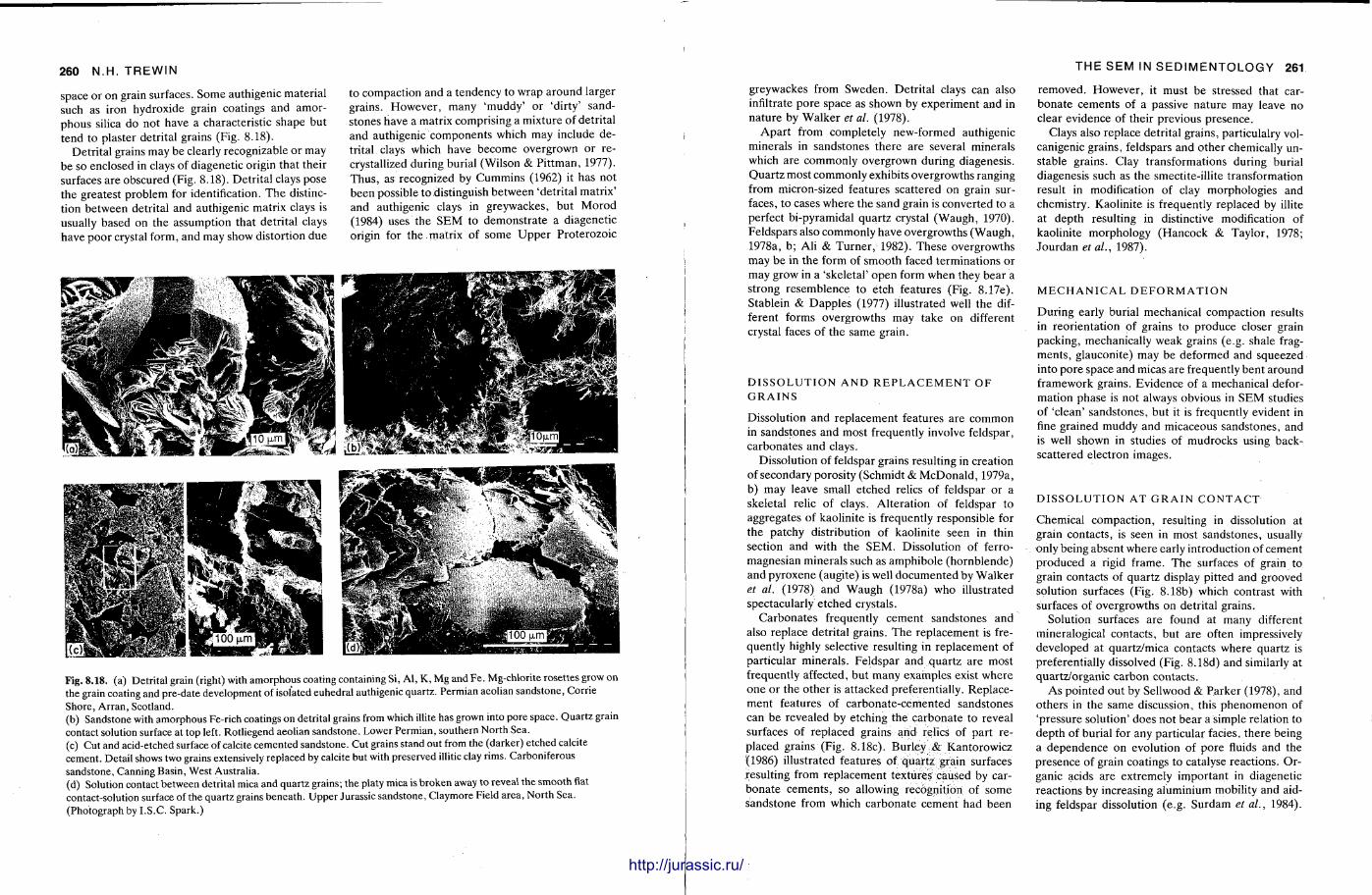
260 N.H. TREWIN
space or on grain surfaces. Some authigenic material such as iron hydroxide grain coatings and amorphous silica do not have a characteristic shape but tend to plaster detrital grains (Fig. 8.18).
Detri tal grains may be clearly recognizable or may be so enclosed in clays of diagenetic origin that their surfaces are obscured (Fig. 8.18). Detri tal clays pose the greatest problem for identification. T h e distinction between detrital and authigenic matrix clays is usually based on the assumption that detrital clays have poor crystal form, and may show distortion due
to compaction and a tendency to wrap around larger grains. However , many 'muddy ' or 'dirty' sandstones have a matrix comprising a mixture of detrital and authigenic components which may include detrital clays which have become overgrown or recrystallized during burial (Wilson & Pi t tman, 1977). Thus , as recognized by Cummins (1962) it has not been possible to distinguish between 'detrital matr ix ' and authigenic clays in greywackes, but Morod (1984) uses the S E M to demonst ra te a diagenetic origin for the matrix of some Uppe r Proterozoic
Fig. 8.18. (a) Detrital grain (right) with amorphous coating containing Si, Al, K, Mg and Fe. Mg-chlorite rosettes grow on the grain coating and pre-date development of isolated euhedral authigenic quartz. Permian aeolian sandstone, Corrie Shore, Arran, Scotland. (b) Sandstone with amorphous Fe-rich coatings on detrital grains from which illite has grown into pore space. Quartz grain contact solution surface at top left. Rotliegend aeolian sandstone. Lower Permian, southern North Sea. (c) Cut and acid-etched surface of calcite cemented sandstone. Cut grains stand out from the (darker) etched calcite cement. Detail shows two grains extensively replaced by calcite but with preserved illitic clay rims. Carboniferous sandstone, Canning Basin, West Australia. (d) Solution contact between detrital mica and quartz grains; the platy mica is broken away to reveal the smooth flat contact-solution surface of the quartz grains beneath. Upper Jurassic sandstone, Claymore Field area, North Sea. (Photograph by I.S.C. Spark.)
greywackes from Sweden. Detri tal clays can also infiltrate pore space as shown by experiment and in nature by Walker et al. (1978).
Apar t from completely new-formed authigenic minerals in sandstones there are several minerals which are commonly overgrown during diagenesis. Quar tz most commonly exhibits overgrowths ranging from micron-sized features scattered on grain surfaces, to cases where the sand grain is converted to a perfect bi-pyramidal quartz crystal (Waugh, 1970). Feldspars also commonly have overgrowths (Waugh, 1978a, b ; Ali & Turner , 1982). These overgrowths may be in the form of smooth faced terminat ions or may grow in a 'skeletal ' open form when they bear a strong resemblence to etch features (Fig. 8.17e). Stablein & Dapples (1977) illustrated well the different forms overgrowths may take on different crystal faces of the same grain.
D I S S O L U T I O N A N D R E P L A C E M E N T O F G R A I N S
Dissolution and replacement features are common in sandstones and most frequently involve feldspar, carbonates and clays.
Dissolution of feldspar grains resulting in creation of secondary porosity (Schmidt & McDonald , 1979a, b) may leave small etched relics of feldspar or a skeletal relic of clays. Al terat ion of feldspar to aggregates of kaolinite is frequently responsible for the patchy distribution of kaolinite seen in thin section and with the SEM. Dissolution of ferro-magnesian minerals such as amphibole (hornblende) and pyroxene (augite) is well documented by Walker et al. (1978) and Waugh (1978a) who illustrated spectacularly etched crystals.
Carbonates frequently cement sandstones and also replace detrital grains. T h e replacement is frequently highly selective resulting in replacement of particular minerals. Feldspar and quartz are most frequently affected, but many examples exist where one or the other is at tacked preferentially. Replacement features of carbonate-cemented sandstones can be revealed by etching the carbonate to reveal surfaces of replaced grains and relics of part replaced grains (Fig. 8.18c). Burley & Kantorowicz (1986) illustrated features of quartz grain surfaces resulting from replacement textures caused by carbonate cements , so allowing recognition of some sandstone from which carbonate cement had been
THE SEM IN SEDIMENTOLOGY 261
M E C H A N I C A L D E F O R M A T I O N
During early burial mechanical compaction results in reorientat ion of grains to produce closer grain packing, mechanically weak grains (e.g. shale fragments , glauconite) may be deformed and squeezed into pore space and micas are frequently bent around framework grains. Evidence of a mechanical deformation phase is not always obvious in SEM studies of 'clean' sandstones, but it is frequently evident in fine grained muddy and micaceous sandstones, and is well shown in studies of mudrocks using back-scattered electron images.
D I S S O L U T I O N A T G R A I N C O N T A C T
Chemical compact ion, resulting in dissolution at grain contacts, is seen in most sandstones, usually only being absent where early introduction of cement produced a rigid frame. The surfaces of grain to grain contacts of quar tz display pitted and grooved solution surfaces (Fig. 8.18b) which contrast with surfaces of overgrowths on detrital grains.
Solution surfaces are found at many different mineralogical contacts, but are often impressively developed at quartz/mica contacts where quartz is preferentially dissolved (Fig. 8.18d) and similarly at quartz/organic carbon contacts .
As pointed out by Sellwood & Parker (1978), and others in the same discussion, this phenomenon of 'pressure solution' does not bear a simple relation to depth of burial for any particular facies, there being a dependence on evolution of pore fluids and the presence of grain coatings to catalyse reactions. Organic acids are extremely important in diagenetic reactions by increasing aluminium mobility and aiding feldspar dissolution (e.g. Surdam et al., 1984).
removed. However , it must be stressed that carbonate cements of a passive nature may leave no clear evidence of their previous presence.
Clays also replace detrital grains, particulalry vol-canigenic grains, feldspars and other chemically unstable grains. Clay transformations during burial diagenesis such as the smectite-illite transformation result in modification of clay morphologies and chemistry. Kaolinite is frequently replaced by illite at depth resulting in distinctive modification of kaolinite morphology (Hancock & Taylor, 1978; Jourdan etal., 1987).
http://jurassic.ru/
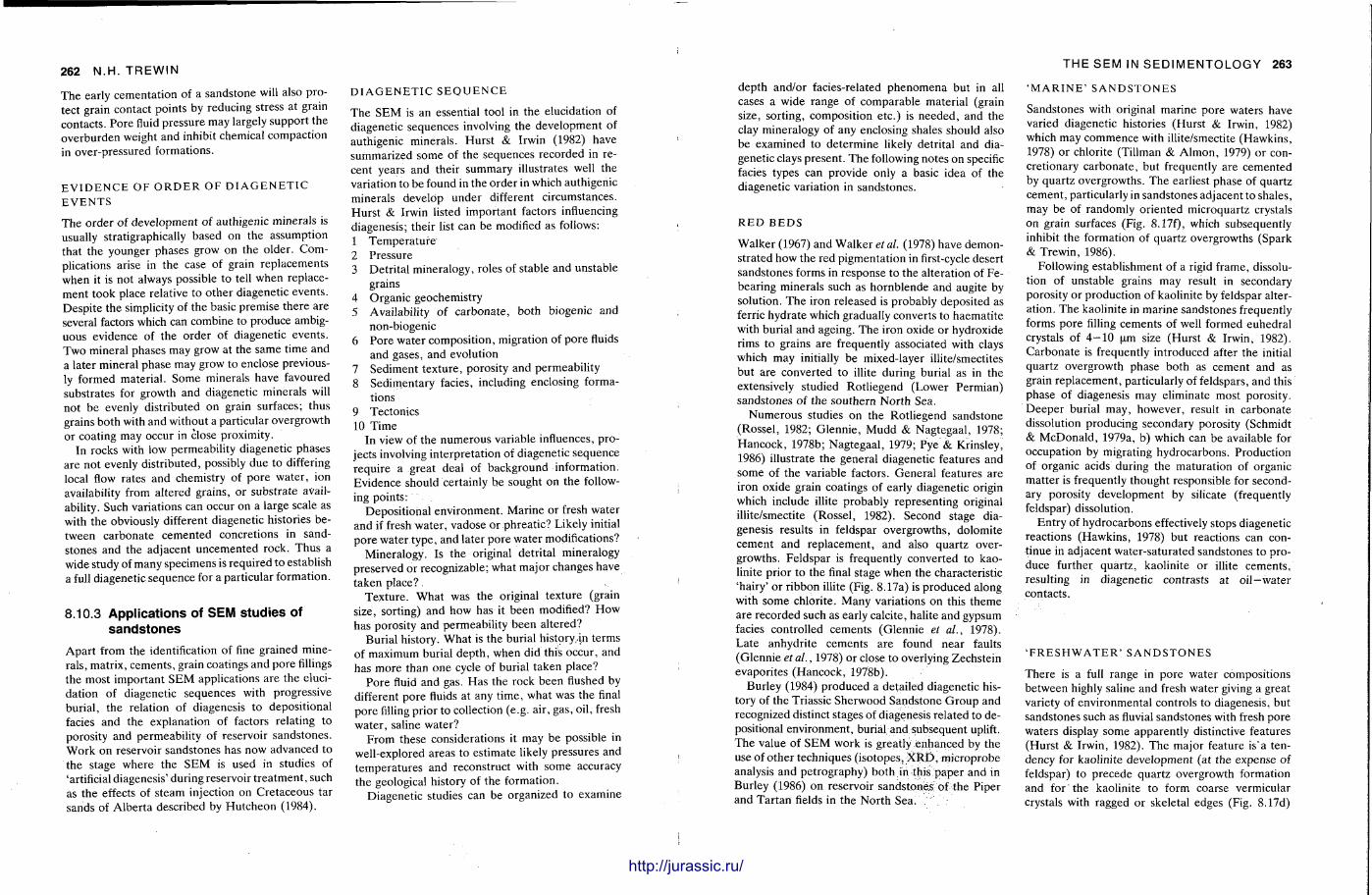
262 N.H. TREWIN
The early cementat ion of a sandstone will also protect grain contact points by reducing stress at grain contacts. Pore fluid pressure may largely support the overburden weight and inhibit chemical compaction in over-pressured formations.
E V I D E N C E O F O R D E R O F D I A G E N E T I C E V E N T S
The order of development of authigenic minerals is usually stratigraphically based on the assumption that the younger phases grow on the older. Complications arise in the case of grain replacements when it is not always possible to tell when replacement took place relative to o ther diagenetic events . Despi te the simplicity of the basic premise there are several factors which can combine to produce ambiguous evidence of the order of diagenetic events . Two mineral phases may grow at the same time and a later mineral phase may grow to enclose previously formed material . Some minerals have favoured substrates for growth and diagenetic minerals will not be evenly distributed on grain surfaces; thus grains both with and without a particular overgrowth or coating may occur in close proximity.
In rocks with low permeability diagenetic phases a re not evenly distr ibuted, possibly due to differing local flow rates and chemistry of pore water , ion availability from altered grains, or substrate availability. Such variations can occur on a large scale as with the obviously different diagenetic histories between carbonate cemented concret ions in sandstones and the adjacent uncemented rock. Thus a wide study of many specimens is required to establish a full diagenetic sequence for a particular formation.
8.10.3 Appl icat ions of SEM studies of sandstones
Apar t from the identification of fine grained minerals, matrix, cements , grain coatings and pore fillings the most important S E M applications are the elucidation of diagenetic sequences with progressive burial , the relation of diagenesis to depositional facies and the explanation of factors relating to porosity and permeability of reservoir sandstones. Work on reservoir sandstones has now advanced to the stage where the S E M is used in studies of 'artificial diagenesis ' during reservoir t rea tment , such as the effects of steam injection on Cretaceous tar sands of Alberta described by Hutcheon (1984).
D I A G E N E T I C S E Q U E N C E
The SEM is an essential tool in the elucidation of diagenetic sequences involving the development of authigenic minerals . Hurs t & Irwin (1982) have summarized some of the sequences recorded in recent years and their summary illustrates well the variation to be found in the order in which authigenic minerals develop under different circumstances. Hurs t & Irwin listed important factors influencing diagenesis; their list can be modified as follows: 1 Tempera tu re 2 Pressure 3 Detri tal mineralogy, roles of stable and unstable
grains 4 Organic geochemistry 5 Availability of carbonate , both biogenic and
non-biogenic 6 Pore water composit ion, migration of pore fluids
and gases, and evolution 7 Sediment texture , porosity and permeabil i ty 8 Sedimentary facies, including enclosing forma
tions 9 Tectonics 10 Time
In view of the numerous variable influences, projects involving interpretat ion of diagenetic sequence require a great deal of background information. Evidence should certainly be sought on the following points :
Deposi t ional environment . Marine or fresh water and if fresh water , vadose or phreatic? Likely initial pore water type, and later pore water modifications?
Mineralogy. Is the original detrital mineralogy preserved or recognizable; what major changes have taken place?
Texture . Wha t was the original texture (grain size, sorting) and how has it been modified? H o w has porosity and permeabil i ty been al tered?
Burial history. Wha t is the burial history.ln terms of maximum burial depth , when did this occur, and has more than one cycle of burial taken place?
Pore fluid and gas. Has the rock been flushed by different pore fluids at any t ime, what was the final pore filling prior to collection (e.g. air, gas, oil, fresh water , saline water?
F rom these considerations it may be possible in well-explored areas to est imate likely pressures and tempera tures and reconstruct with some accuracy the geological history of the formation.
Diagenetic studies can be organized to examine
WWII!
THE SEM IN SEDIMENTOLOGY 263
depth and/or facies-related phenomena but in all cases a wide range of comparable material (grain size, sorting, composition etc .) is needed , and the clay mineralogy of any enclosing shales should also be examined to de termine likely detrital and diagenetic clays present . The following notes on specific facies types can provide only a basic idea of the diagenetic variation in sandstones.
R E D B E D S
Walker (1967) and Walker et al. (1978) have demonstrated how the red pigmentat ion in first-cycle desert sandstones forms in response to the alteration of Fe-bearing minerals such as hornblende and augite by solution. The iron released is probably deposited as ferric hydrate which gradually converts to haemati te with burial and ageing. The iron oxide or hydroxide rims to grains are frequently associated with clays which may initially b e mixed-layer illite/smectites but are converted to illite during burial as in the extensively studied Rotliegend (Lower Permian) sandstones of the southern Nor th Sea.
Numerous studies on the Rotliegend sandstone (Rossel , 1982; Glennie , Mudd & Nagtegaal , 1978; Hancock , 1978b; Nagtegaal , 1979; Pye & Krinsley, 1986) illustrate the general diagenetic features and some of the variable factors. General features are iron oxide grain coatings of early diagenetic origin which include illite probably representing original illite/smectite (Rossel , 1982). Second stage diagenesis results in feldspar overgrowths, dolomite cement and replacement , and also quar tz overgrowths. Feldspar is frequently converted to kaolinite prior to the final stage when the characteristic 'hairy ' or r ibbon illite (Fig. 8.17a) is produced along with some chlorite. Many variations on this theme are recorded such as early calcite, halite and gypsum facies controlled cements (Glennie et al., 1978). La te anhydrite cements are found near faults (Glennie et al., 1978) or close to overlying Zechstein evaporites (Hancock, 1978b).
Burley (1984) produced a detailed diagenetic history of the Triassic Sherwood Sandstone G r o u p and recognized distinct stages of diagenesis related to depositional environment, burial and subsequent uplift. The value of S E M work is greatly enhanced by the use of o ther techniques (isotopes, X R D , microprobe analysis and petrography) both in this paper and in Burley (1986) on reservoir sandstones of the Piper and Tar tan fields in the Nor th Sea. .""
' M A R I N E ' S A N D S T O N E S
Sandstones with original mar ine pore waters have varied diagenetic histories (Hurst & Irwin, 1982) which may commence with illite/smectite (Hawkins, 1978) or chlorite (Tillman & Almon , 1979) or concretionary carbonate , but frequently are cemented by quartz overgrowths. The earliest phase of quartz cement , particularly in sandstones adjacent to shales, may be of randomly oriented microquartz crystals on grain surfaces (Fig. 8.17f), which subsequently inhibit the formation of quartz overgrowths (Spark & Trewin, 1986).
Following establishment of a rigid frame, dissolution of unstable grains may result in secondary porosity or production of kaolinite by feldspar alteration. The kaolinite in marine sandstones frequently forms pore filling cements of well formed euhedral crystals of 4 - 1 0 um size (Hurs t & Irwin, 1982). Carbonate is frequently introduced after the initial quartz overgrowth phase both as cement and as grain replacement , particularly of feldspars, and this phase of diagenesis may eliminate most porosity. Deepe r burial may, however , result in carbonate dissolution producing secondary porosity (Schmidt & McDonald , 1979a, b) which can be available for occupation by migrating hydrocarbons. Production of organic acids during the maturat ion of organic matter is frequently thought responsible for secondary porosity development by silicate (frequently feldspar) dissolution.
Ent ry of hydrocarbons effectively stops diagenetic reactions (Hawkins, 1978) but reactions can continue in adjacent water-saturated sandstones to produce further quar tz , kaolinite or illite cements , resulting in diagenetic contrasts at oil—water contacts.
' F R E S H W A T E R ' S A N D S T O N E S
There is a full range in pore water compositions between highly saline and fresh water giving a great variety of environmental controls to diagenesis, but sandstones such as fluvial sandstones with fresh pore waters display some apparently distinctive features (Hurst & Irwin, 1982). The major feature is"a tendency for kaolinite development (at the expense of feldspar) to precede quartz overgrowth formation and for the kaolinite to form coarse vermicular crystals with ragged or skeletal edges (Fig. 8.17d)
http://jurassic.ru/
264 N.H. TREWIN
which may have grown more rapidly than the characteristic 'mar ine ' form of kaolinite. However , it is important to recognize that a great many sandstones deposited under shallow marine conditions are subsequently flushed by fresh water from adjacent land areas during early burial or later uplift.
Carbonates may be developed at more than one stage in the diagenetic history, ranging from pedo-genic carbonate of caliche soils, or early pre-com-paction carbonate nodules through to late diagenetic calcite, dolomite or siderite precipitation post-dating quartz cementat ion and occuring at depths of 2—3 km. Flushing of. originally marine sandstones by fresh water will frequently superimpose new diagenetic features, thus formations involved in uplift and reburial can possess complex diagenetic histories.
P O R O S I T Y A N D ^ P E R M E A B I LITY
The permeability of a sandstone is related to the size and shape of pore throats which connect larger pore volumes in a sandstone, the tortuosity of pores , and the specific surface area within pore space. The S E M is ideal for examination of pore geometry by means of pore casts and also ideal for viewing the factors which serve to reduce porosity and permeability in sandstone. One of the most obvious examples of permeabili ty reduction by the formation of authigenic minerals within pore space is that provided by the illite diagenesis of the Rotl iegend sandstone of the southern North Sea where delicate illite crystals bridge and block pore throats (Fig. 8.18b), so reducing permeabili ty. The Brent Sandstone (Middle Jurassic, North Sea) displays similar features with illite also responsible for permeability reduction (Hancock & Taylor, 1978; Blanche & Whi taker , 1978), and the Magnus reservoir (Uppe r Jurassic, Nor th Sea) is similarly affected (McHardy et al., 1982). Kaolinite is not usually so detr imental to permeability as illite since it has a larger grain size, and smaller surface area (Fig. 8.17c) so that pore tortuosity and water absorption on the clay surface are not so great. Kaolinite also tends to be more patchy in its distribution in the rock. S E M studies can be valuable in the assessment of micro-porosity in reservoirs as in the case of porcelaneous cement of opal , microquartz and montmoril lonite described from Miocene turbidite sandstones of the Los Angeles Basin by Sears (1984).
As oil migrates into a reservoir diagenesis is arrested as in the case of the Brent Sandstone (Hancock &
Taylor, 1978; Sommer , 1978) where it can be shown that oil migrated into place synchronously with illite formation, there being a downward increase in illite within the reservoir. Thus the relative timing of generat ion and migration of hydrocarbons during diagenesis can be determined and predictions can be made on reservoir quality with respect to facies, geographical area and depth of burial.
Porosity can be observed with the S E M and, by use of image analysis equipment on polished sections, particularly in the backscattered mode , can be determined quantitatively. Pore surfaces are best examined on rough broken rock surfaces. Pore throat size and pore connection is most easily studied using pore casts (Fig. 8.21).
C O N C L U S I O N
From these few examples it is apparent that the diagenesis of any sandstone formation must be studied with reference to all available information on facies; pore fluids, burial history and composition. Utilization of S E M techniques can greatly aid explanation of porosity and permeabili ty parameters , relating them to depositional and diagenetic factors by examination of pore morphologies and fillings.
8.11 L I M E S T O N E S A N D D O L O M I T E S
8.11.1 General
Utilization of the S E M for the study of l imestones is most valuable in the examination of fine-grained porous limestones such as chalk (Scholle, 1977) and for tracing the evolution of cement and replacement fabrics in Recent to sub-Recent carbonates (Bathurst, 1975; Folk, 1974a; James et al., 1976; Wilkinson et al., 1982). In studies of modern fine-grained carbonate sediments the morphologies and origins of grains can be determined (Hay et al., 1970) and detail of biogenic particles more easily recognized.
Textures and pore geometry of dolomitized and dedolomitized sediments are also suitable for examinat ion as in examples of Silurian dolomite diagenesis in the Lockport Format ion , U S A (Shukla & Fre idman, 1983), dolomitized Cretaceous chalk of E u r o p e (Jorgensen, 1983) and recent Austral ian Coorong dolomites (Von Der Borch & Lock, 1979).
For a general discussion of carbonate petrology,
THE SEM IN SEDIMENTOLOGY 265
Bathurst (1975) provides an excellent account and Scholle (1978) illustrates the use of the S E M in carbonate studies and provides a useful bibliography to selected topics and techniques. A variety of techniques such as thin section, X R D and cathodoluminescence and isotope analysis are all of great value in carbonate studies and the S E M can make a useful contribution in many cases and provides excellent illustrative material .
Only a few examples can be quoted in the space available and these are chosen to illustrate the wide range of use of the S E M in carbonate studies, without a t tempting to review theories on the various examples presented.
8.11.2 Examples
C A R B O N A T E G R A I N S
Unconsolidated carbonate sediments can be examined as scattered grain mounts for the identification of fine carbonate grains. This technique is useful for the identification of biogenic particles as shown experimentally by Hay et al. (1970) who crushed examples of known invertebrate material and were able to recognize distinctive skeletal morphologies in fine sands and even in some grains as small as 4 pm. Mount ing the grains in resin and examining polished and etched surfaces enabled them to recognize distinctive skeletal internal structures.
The contributions which the fragmentation products of organisms make to carbonate muds , such as aragonite needles derived from the breakdown of the calcified algae Halimeda and Penicillus, and the contribution of coccoliths, discoasters and o ther planktonic organisms to deep sea oozes can be ascertained (illustrations in Scholle, 1978). Alex-andersson (1979) illustrates the contribution that the breakdown products of mussel (Mytilus) shells make to sediments of the Skagerrak, Nor th Sea. A similar process operates in muds of the Ythan Estuary, Nor th Scotland, where characteristic calcite needles and plates are released by the breakdown within the sediment of mussel shell fragments originally contributed to the sediment by the predatory activities of eider ducks feeding on the local mussel beds (Trewin & Welsh, 1976; Fig. 8.19). Calcite needles originating from the breakdown of musse l shells also occur in suspended sediment on the north-eastern U S A Continental shelf (Fitzgerald, Parmenter & M i l l i m a n ,
1979).
Sediments may also be examined for grains of non-biogenic origin such as the 2—20 |xm high-Mg calcite grains precipitated in Lake Mani toba (Canada) illustrated by Last (1982) and the numerous studies of ooids and their structure such as that of Land , Behrens & Frishman (1979) on the ooids of Baffin Bay, Texas , and Sandberg (1975) and Halley (1977) on the ooids of the Great Salt Lake . Sandberg 's study utilizes S E M examination of etched surfaces to show that coarse radial aragonite is of depositional ra ther than recrystallization origin. The S E M provides evidence not available from microscope petrography.
Evidence of aragonite replacement by calcite can also be revealed by SEM preparat ions such as the relic aragonite structures in calcitized Jurassic bivalves illustrated by Sandberg & Hudson (1983).
These and many other studies illustrate the general use of the S E M in studies involving carbona te grains.
C E M E N T A T I O N O F C A R B O N A T E S
There are many cases in which early cementat ion of carbonates occurs in mar ine subtidal and intertidal conditions and in freshwater phreatic and vadose situations. The morphology of the cements produced can ideally be examined using the SEM and much more detail obtained than is possible in thin section. In freshwater solutions with low M g + + concentrat ions there is a tendency for simple rhombs to grow, but in solutions with a high M g + + concentrat ion sideways growth of the crystals may be poi-
Fig. 8.19. Bivalve (Mytilus) shell fragment breaking up to release individual calcite laths into the sediment. From recent intertidal mudflat, Ythan Estuary, North Scotland.
http://jurassic.ru/
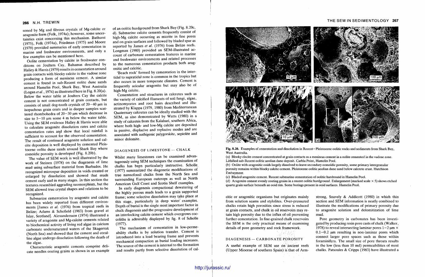
266 N.H. TREWIN
soned by Mg and fibrous crystals of Mg-calcite or aragonite form (Folk, 1974a); however, some uncertainties exist concerning this mechanism. Bathurs t (1975), Folk (1974a), Fr iedman (1975) and Moore (1979) provided summaries of early cementat ion in mar ine and freshwater environments , and only a few examples can be ment ioned here .
Ooli te cementat ion by calcite in freshwater conditions on Joul ters Cay, Bahamas described by Halley & Harr is (1979) results in cementat ion around grain contacts with blocky calcite in the vadose zone producing a form of meniscus cement . A similar cement is found in sub-Recent ooli te dune sands a round Hamel in Pool , Shark Bay, West Austral ia (Logan etal., 1974) as illustrated here in Fig. 8.20(a). Below the water table at Joulters Cay the calcite cement is not concentrated at grain contacts , but consists of small dog-tooth crystals of 20—40 um in isopachous grain coats and in deeper samples scattered rhombohedra of 20—30 um which decrease in size to 5—10 um some 4 m below the wate r table . Using the S E M evidence Halley & Harr is were able to calculate aragonite dissolution rates and calcite cementat ion rates and show that local rainfall is sufficient to account for the observed cementat ion. T h e result of cont inued aragoni te solution and calcite deposition is well displayed by cemented Pleistocene oolite dune sands around Shark Bay where comoldic porosity is developed (Fig. 8.20b).
The value of S E M work is well illustrated by the work of Steinen (1978) on the diagenesis of lime mud using subsurface material from Barbados . H e recognized microspar deposition in voids created or enlarged by dissolution and showed that muds cement early and in many stages. In thin section the textures resembled aggrading neomorphism, but the SEM allowed t rue crystal shapes and relations to be recognized.
Submarine cementat ion by aragonite and calcite has been widely repor ted from different environments [James et al. (1976) from tropical reefs in Belize; Adams & Schofield (1983) from gravel at Islay, Scotland]. Alexandersson (1974) illustrated a variety of aragonite and Mg-calcite cements related to biochemical activity of living red algae in calcium carbonate undersaturated waters of the Skagerrak (Nor th Sea) and showed that the cement and coralline algae undergo dissolution following the death of the algae.
Characteristic aragonite cements comprise delicate needles coating grains as shown in an example
of an oolitic hardground from Shark Bay (Fig. 8.20c, d ) . Submarine calcite cements frequently consist of high-Mg calcite occurring as micrite in fine pores and on grain surfaces and followed by bladed spar as repor ted by James et al. (1976) from Belize reefs. Longman (1980) provided an SEM-illustrated account of carbonate cementat ion features in marine and freshwater environments and related processes to the numerous cementat ion products both arag-onitic and calcitic.
'Beach rock' formed by cementat ion in the intertidal to suprat idai zone is common in the tropics but also occurs in more t empera te cl imates. Cemen t is frequently acicular aragonite but may also be of high-Mg calcite.
Cementa t ion and structures in calcretes such as the variety of calcified filaments of soil fungi, a lgae, act inomycetes and root hairs described and illustrated by Klappa (1979, 1980) from Medi ter ranean Quaternary calcretes can be ideally studied with the S E M , as also demonst ra ted by Wat ts (1980) in a study of calcretes from the Kalahari, southern Africa, where both high- and low-Mg calcite are deposited in passive, displacive and replacive modes and are associated with authigenic palygorskite, sepiolite and minor dolomite .
D I A G E N E S I S O F L I M E S T O N E — C H A L K
Whilst many limestones can be examined advantageously using S E M techniques the examination of chalks has been particularly instructive. Scholle, (1977) summarized the diagenetic modifications of t rue nannofossil chalks from the Nor th Sea and surrounding E u r o p e a n outcrops as well as Nor th American Gulf Coast and Scotia Shelf examples.
In early diagenesis compactional dewatering of the highly porous muds leads to a grain suppor ted frame; some selective dissolution may take place at this s tage, particularly in deep water ' examples. Dep th of burial is the single most important factor in chalk diagenesis and the progressive development of an interlocking calcite cement which overgrows coc-coliths is admirably displayed by fig. 8 of Scholle (1977).
The mechanism of cementat ion in low-permeability chalks is by solution transfer. C e m e n t is introduced into a load bearing frame and prevents mechanical compaction as burial loading increases. T h e source of the cement is internal to the formation and results partly from selective dissolution of cal-
THE SEM IN SEDIMENTOLOGY 267
Fig. 8.20. Examples of cementation and dissolution in Recent—Pleistocene oolitic rocks and sediments from Shark Bay, West Australia. (a) Blocky clacite cement concentrated at grain contacts as a meniscus cement in a oolite cemented in the vadose zone. Lithified sub-Recent oolitic aeolian dune deposit. Carbla Point, Hamelin Pool. (b) Oolite with aragonitic ooids largely dissolved to leave secondary oomoldic porosity, some primary intergranular porosity remains within blocky calcite cement. Pleistocene oolitic aeolian dune sand below calcrete crust. Hutchison Embayment. (c) Bladed aragonite cement. Recent submarine cementation of oolitic hardround in Hamelin Pool. (d) Aragonite cement evenly coating grains in a recent oolitic hardground. Enlargement (marked scale x 5) shows etched quartz grain surface beneath an ooid rim. Some borings present in ooid surfaces. Hamelin Pool.
citic or aragonitic organisms but originates mainly from solution seams and stylolites. Over-pressured chalks retain high porosities since stress is reduced at grain contacts , and chalk in oil reservoirs may retain high porosity due to the influx of oil preventing further cementat ion. In fine-grained chalk reservoirs the S E M is the only practical means of examining details of pore geometry and rock framework.
D I A G E N E S I S — C A R B O N A T E P O R O S I T Y
A useful example of S E M use on ancient reefs (Upper Miocene of southern Spain) is that of Arm
strong, Snavely & Addicot t (1980) in which thin section and S E M information is neatly combined to illustrate the modifications of primary porosity due to aragonite solution and dolomitization of lime mud.
Pore geometry in carbonates has been investigated by producing resin pore casts of chalk (Walker , 1978) to reveal intersecting laminar pores 1—2 um x 0.1—0.2 pm resulting in non-laminar pores which connect larger pore spaces such as those within foraminifera. The small size of pore throats results in the low (less than 10 md) permeabili t ies of most chalks. Patsoules & Cripps (1983) have illustrated a
http://jurassic.ru/
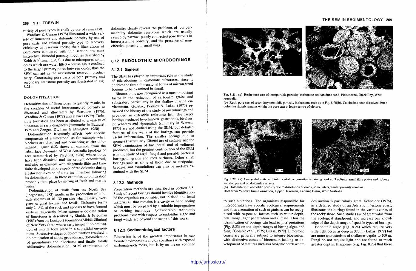
268 N.H. TREWIN
variety of pore types in chalk by use of resin casts. Wardlaw & Cassan (1978) illustrated a wide var
iety of l imestone and dolomite porosity by use of pore casts and related porosity type to recovery efficiency in reservoir rocks; their illustrations of pore casts compared with thin section are most instructive. Bimodal porosity in oolites described by Keith & Pit tman (1983) is due to micropores within ooids which are water filled whereas gas is confined to the larger primary pores between ooids, thus the SEM can aid in the assessment reservoir productivity. Contrast ing pore casts of both primary and secondary l imestone porosity are illustrated in Fig. 8.21.
D O L O M I T I Z A T I O N
Dolomitization of limestones frequently results in the creation of useful interconnected porosity as discussed and illustrated by Wardlaw (1976), Wardlaw & Cassan (1978) and Davies (1979). Dolomite formation has been at tr ibuted to a variety of processes in early diagenesis (summaries in Bathurst, 1975 and Zenger , D u n h a m & Ethington, 1980).
Dolomitization frequently affects only specific components of a l imestone, as for example when bioclasts are dissolved and cementing calcite dolomitized. Figure 8.22 shows an example from the subsurface Devonian of West Austral ia (geology of area summarized by Playford, 1980) where ooids have been dissolved and the cement dolomitized, and also an example with diagenetic illite and kaolinite developed in pore space of the dolomite during freshwater invasion of a marine limestone following its dolomitization. In these examples dolomitization probably took place by mixing of fresh and marine water .
Dolomitization of chalk from the Nor th Sea (Jorgensen, 1983) results in the product ion of dolomite rhombs of 10—30 urn size which clearly overgrow original texture and fossils. Dolomi te forms only 2—8% of the rock and appears to have formed early in diagenesis. M o r e extensive dolomitization of limestones is described by Shukla & Fr iedman (1983) from the Lockport Formation (Middle Silurian) of New York State where early incipient dolomitization of micrite took place in a supratidal environment . Successive stages of dolomitization resulted in dolomitization of all the groundmass , dolomitization of groundmass and allochems and finally totally obliterative dolomitization. S E M examination of
dolomites clearly reveals the problems of low permeability dolomite reservoirs which are usually caused by nar row, poorly connected pore throats in intercrystalline porosity, and the presence of noneffective porosity in small vugs.
8.12 E N O O L O T H I C M I C R O B O R I N G S
8.12.1 General The S E M has played an important role in the study of microborings in carbonate substrates , since it enables the three-dimensional forms of micron-sized borings to be examined in detail .
Bioerosion is now recognized as a most impor tant factor in the reduction of carbonate grains and substrates , particularly in the shallow mar ine environment . Golubic , Perkins & Lukas (1975) reviewed the history of the study of microborings and provided an extensive reference list. T h e larger borings produced by echinoids, gast ropods, bivalves, polychaetes and sipunculids (summary in W a r m e , 1975) a re not studied using the S E M , but detailed features of the walls of the borings can provide useful information. T h e smaller borings due to sponges (particularly Cliona) are of suitable size for S E M examination of fine detail and of sediment produced, but the greatest contr ibution of the S E M is in the study of algal, fungal and possible bacterial borings in grains and rock surfaces. O the r small borings such as some of those due to cirripedes, bryozoa and foraminifera can also be usefully examined with the S E M .
8.12.2 Methods Prepara t ion methods are described in Section 8.5. Study of recent borings should involve identification of the organism responsible, but iii dead and fossil material all that remains is a cavity or filled boring which must be p repared by a suitable impregnat ion or etching technique. Considerable taxonomic problems exist with respect t o endolithic algae and fungi which a re beyond the scope of this work .
8.12.3 Sedimentological factors
Bioerosion is of the greatest impor tance in carbona te environments and on coastlines with exposed carbonate-rich rocks, but is by no means confined
THE SEM IN SEDIMENTOLOGY 269
Fig. 8.21. (a) Resin pore-cast of interparticle porosity; carbonate aeolian dune sand, Pleistocene, Shark Bay, West Australia. (b) Resin pore cast of secondary oomoldic porosity in the same rock as in Fig. 8.20(b). Calcite has been dissolved, but a dolomite rhomb remains within the pore cast at lower centre of picture.
Fig. 8.22. (a) Coarse dolomite with intercrystalline porosity containing books of kaolinite; small illite plates and ribbons are also present on dolomite surfaces. (b) Dolomite with oomoldic porosity due to dissolution of ooids, some intergranular porosity remains. Both from Yellow Drum Formation, Upper Devonian, Canning Basin, West Australia.
to such situations. The organisms responsible for microborings have specific ecological requirements and thus a zonation of such organisms can be recognized with respect to factors such as water depth , tidal range , light penetra t ion and climate. Thus the identification of borings can lead to interpretat ions (Fig. 8.23) on the depth ranges of boring algae and fungi (Golubic et al., 1975; Lukas , 1979). L imes tone coasts are generally subject to intense bioerosion, with distinctive zones of bioerosion leading to development of features such as a biogenic notch where
destruction is particularly great . Schneider (1976), in a detailed study of an Adriat ic l imestone coast, illustrates the borings found in the various zones of the rocky shore. Such studies are of great value from the ecological s tandpoint , and increase our knowledge of the depth range of specific types of borings.
Endoli thic algae (Fig. 8.24) which require very little light occur as deep as 370 m (Lukas , 1979) but are more characteristic of shallower depths to 100 m. Fungi do not require light and are found to much greater depths . It appears (e.g. Fig. 8.23) that there
http://jurassic.ru/
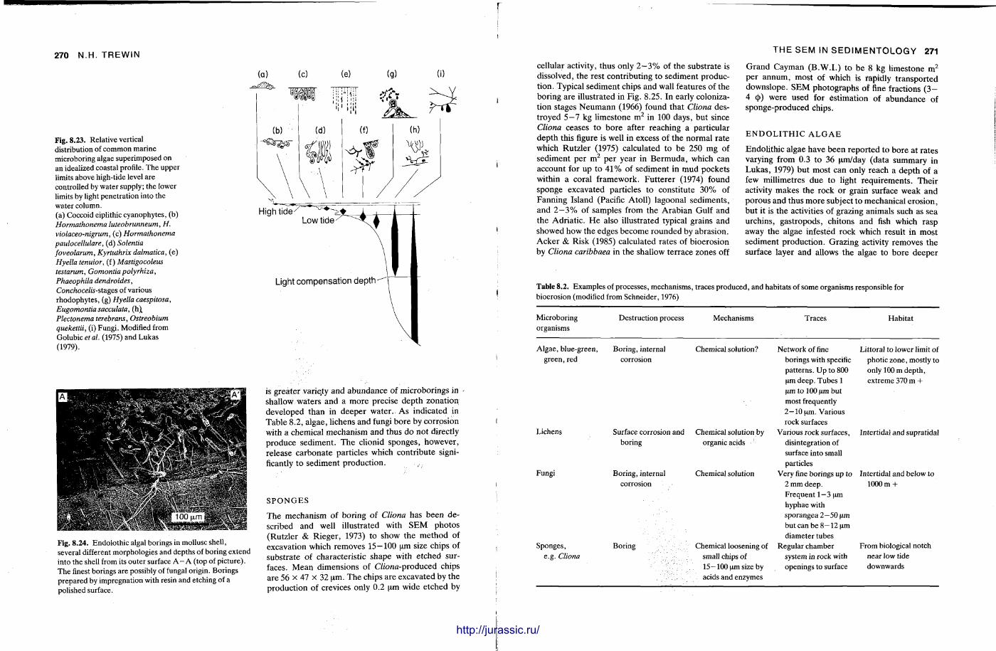
270 N.H. TREWIN
Fig. 8.23. Relative vertical distribution of common marine microboring algae superimposed on an idealized coastal profile. The upper limits above high-tide level are controlled by water supply; the lower limits by light penetration into the water column. (a) Coccoid eiplithiccyanophytes, (b) Hormathonema luteobrunneum, H. violaceo-nigrum, (c) Hormathonema paulocellulare, (d) Solentia foveolarum, Kyrtuthrix dalmatica, (e) Hyella tenuior, (f) Mastigocoleus testarum, Gomontiapolyrhiza, Phaeophila dendroides, Conchocelis-st&ges of various rhodophytes, (g) Hyella caespitosa, Eugomontiasdcculata, (h\ Plectonema terebrans, Ostreobium quekettii, (i) Fungi. Modified from Golubic et al. (1975) and Lukas (1979).
High t ide/ A i Low t i d e / ^
Light compensation depth
Fig. 8.24. Endolothic algal borings in mollusc shell, several different morphologies and depths of boring extend into the shell from its outer surface A - A (top of picture). The finest borings are possibly of fungal origin. Borings prepared by impregnation with resin and etching of a polished surface.
is greater variety and abundance of microborings in shallow waters and a more precise depth zonat ion developed than in deepe r water . A s indicated in Table 8.2, algae, lichens and fungi bore by corrosion with a chemical mechanism and thus do not directly produce sediment . T h e clionid sponges , however , release carbonate particles which contr ibute significantly to sediment product ion.
S P O N G E S
The mechanism of boring of Cliona has been described and well illustrated with S E M photos (Rutzler & Rieger, 1973) to show the method of excavation which removes 15—100 um size chips of substrate of characteristic shape with etched surfaces. Mean dimensions of C7/ona-produced chips are 56 x 47 x 32 um. The chips are excavated by the product ion of crevices only 0.2 um wide etched by
THE SEM IN SEDIMENTOLOGY 271
cellular activity, thus only 2 - 3 % of the substrate is dissolved, the rest contributing to sediment production. Typical sediment chips and wall features of the boring are illustrated in Fig. 8.25. In early colonization stages Neumann (1966) found that Cliona destroyed 5—7 kg limestone m 2 in 100 days, but since Cliona ceases to bore after reaching a particular depth this figure is well in excess of the normal ra te which Rutzler (1975) calculated to be 250 mg of sediment per m 2 per year in Bermuda , which can account for up to 4 1 % of sediment in mud pockets within a coral framework. Fut terer (1974) found sponge excavated particles to constitute 30% of Fanning Island (Pacific Atoll) lagoonal sediments , and 2—3% of samples from the Arabian Gulf and the Adriat ic . H e also illustrated typical grains and showed how the edges become rounded by abrasion. Acker & Risk (1985) calculated rates of bioerosion by Cliona caribbaea in the shallow terrace zones off
Grand Cayman (B .W.I . ) to be 8 kg limestone m 2
per annum, most of which is rapidly t ransported downslope. S E M photographs of fine fractions ( 3 -4 c[>) were used for est imation of abundance of sponge-produced chips.
E N D O L I T H I C A L G A E
Endoli thic algae have been repor ted to bore at rates varying from 0.3 t o 36 um/day (data summary in Lukas , 1979) but most can only reach a depth of a few millimetres due to light requirements . Their activity makes t he rock or grain surface weak and porous and thus more subject to mechanical erosion, but it is the activities of grazing animals such as sea urchins, gastropods, chitons and fish which rasp away the algae infested rock which result in most sediment product ion. Grazing activity removes the surface layer and allows the algae to bore deeper
Table 8.2. Examples of processes, mechanisms, traces produced, and habitats of some organisms responsible for bioerosion (modified from Schneider, 1976)
Microboring Destruction process Mechanisms Traces Habitat organisms
Algae, blue-green, Boring, internal Chemical solution? Network of fine Littoral to lower limit of green,red corrosion borings with specific
patterns. Up to 800 urn deep. Tubes 1 urn to 100 um but most frequently 2—10 um. Various rock surfaces
photic zone, mostly to only 100 m depth, extreme 370 m +
Lichens Surface corrosion and Chemical solution by Various rock surfaces, Intertidal and supratidal boring organic acids disintegration of
surface into small particles
Fungi Boring, internal Chemical solution Very fine borings up to Intertidal and below to corrosion 2 mm deep.
Frequent 1-3 urn hyphae with sporangea 2 -50 \im but can be 8—12 urn diameter tubes
1000 m +
Sponges, Boring Chemical loosening of Regular chamber From biological notch e.g. Cliona small chips of system in rock with near low tide
15—100 um size by openings to surface downwards acids and enzymes
Jjjliil i i i liilh, http://jurassic.ru/
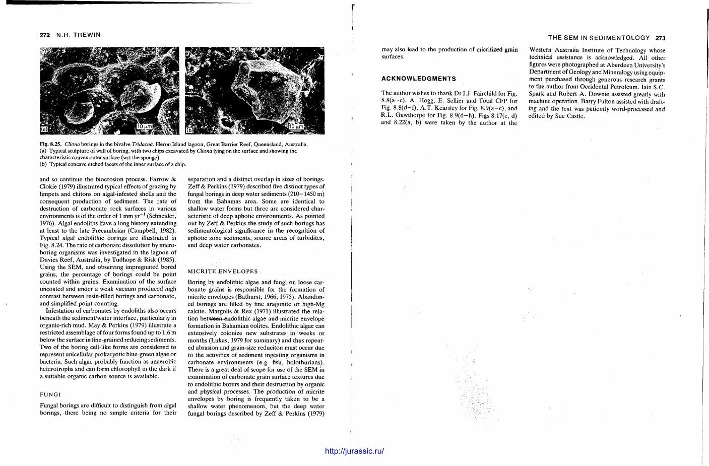
272 N.H. TREWIN
Fig. 8.25. Cliona borings in the bivalve Tridacna. Heron Island lagoon, Great Barrier Reef, Queensland, Australia. (a) Typical sculpture of wall of boring, with two chips excavated by Cliona lying on the surface and showing the characteristic convex outer surface (wrt the sponge). (b) Typical concave etched facets of the inner surface of a chip.
and so continue the bioerosion process. Farrow & Clokie (1979) illustrated typical effects of grazing by limpets and chitons on algal-infested shells and the consequent product ion of sediment. The ra te of destruction of carbonate rock surfaces in various environments is of the order of 1 mm y r _ 1 (Schneider, 1976). Algal endoliths Have a long history extending at least to the late Precambrian (Campbel l , 1982). Typical algal endolithic borings are illustrated in Fig. 8.24. T h e rate of carbonate dissolution by microboring organisms was investigated in the lagoon of Davies Reef, Austral ia , by Tudhope & Risk (1985). Using the S E M , and observing impregnated bored grains, the percentage of borings could be point counted within grains. Examinat ion of the surface uncoated and under a weak vacuum produced high contrast between resin-filled borings and carbonate , and simplified point-counting.
Infestation of carbonates by endoliths also occurs benea th the sediment/water interface, particularly in organic-rich mud. May & Perkins (1979) illustrate a restricted assemblage of four forms found up to 1.6 m below the surface in fine-grained reducing sediments . Two of the boring cell-like forms are considered to represent unicellular prokaryotic blue-green algae or bacteria. Such algae probably function as anaerobic he terot rophs and can form chlorophyll in the dark if a suitable organic carbon source is available.
F U N G I
Fungal borings are difficult to distinguish from algal borings, there being no simple criteria for their
separat ion and a distinct overlap in sizes of borings. Zeff & Perkins (1979) described five distinct types of fungal borings in deep water sediments (210—1450 m) from the Bahamas area. Some are identical to shallow water forms but three are considered characteristic of deep aphotic environments . As pointed out by Zeff & Perkins the study of such borings has sedimentological significance in the recognition of aphotic zone sediments , source areas of turbidites, and deep water carbonates .
M I C R I T E E N V E L O P E S
Boring by endolithic algae and fungi on loose carbonate grains is responsible for the formation of micrite envelopes (Bathurst , 1966,1975). Abandoned borings are filled by fine aragonite or high-Mg calcite. Margolis & Rex (1971) illustrated the relation between endolithic algae and micrite envelope formation in Bahamian oolites. Endoli thic algae can extensively colonize new substrates in weeks or months (Lukas , 1979 for summary) and thus repeated abrasion and grain-size reduciton must occur due to the activities of sediment ingesting organisms in carbonate environments (e.g. fish, holothurians) . The re is a great deal of scope for use of the S E M in examination of carbonate grain surface textures due to endolithic borers and their destruction by organic and physical processes. The production of micrite envelopes by boring is frequently taken to be a shallow water p h e n o m e n o m , but the deep water fungal borings described by Zeff & Perkins (1979)
ii iimiiii
THE SEM IN SEDIMENTOLOGY 273
may also lead to the production of micritized grain surfaces.
ACKNOWLEDGMENTS
The author wishes to thank Dr I.J. Fairchild for Fig. 8 . 8 ( a - c ) , A . Hogg, E . Sellier and Total C F P for Fig. 8 .8 (d - f ) , A . T . Kearsley for Fig. 8 . 9 ( a - c ) , and R . L . Gawthorpe for Fig. 8 . 9 ( d - h ) . Figs 8.17(c, d) and 8.22(a, b) were taken by the author at the
Western Australia Institute of Technology whose technical assistance is acknowledged. AH other figures were photographed at Aberdeen University's Depa r tmen t of Geology and Mineralogy using equipment purchased through generous research grants to the author from Occidental Petroleum. Iain S.C. Spark and Rober t A . Downie assisted greatly with machine operat ion. Barry Fulton assisted with drafting and the text was patiently word-processed and edited by Sue Castle.
http://jurassic.ru/
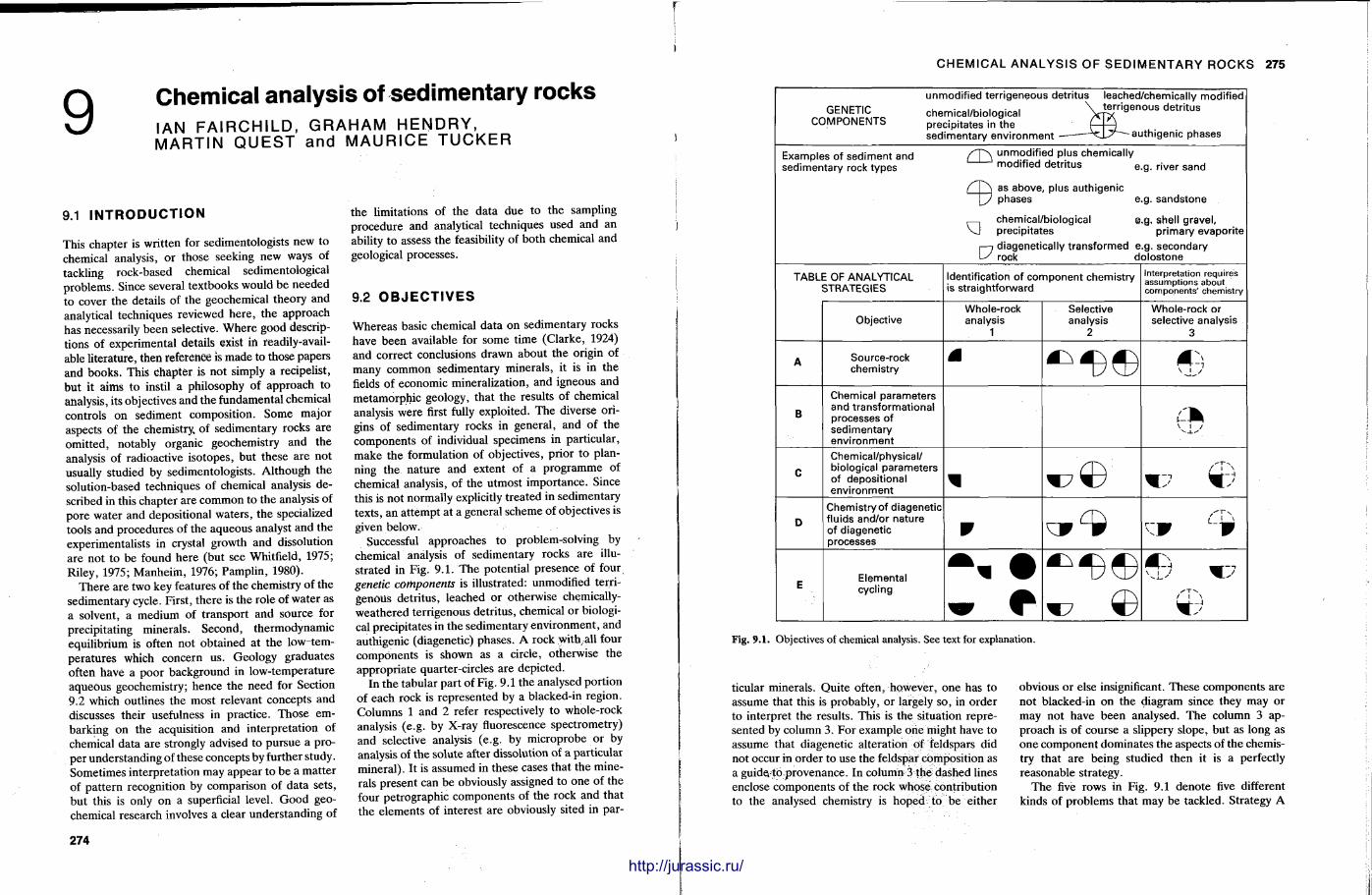
9 Chemical analysis of sedimentary rocks IAN FAIRCHILD, GRAHAM HENDRY, MARTIN QUEST and MAURICE TUCKER
9.1 I N T R O D U C T I O N
This chapter is writ ten for sedimentologists new to chemical analysis, or those seeking new ways of tackling rock-based chemical sedimentological problems. Since several textbooks would b e needed to cover the details of the geochemical theory and analytical techniques reviewed he re , the approach has necessarily been selective. W h e r e good descriptions of experimental details exist in readily-available literature, then reference is made to those papers and books . This chapter is not simply a recipelist, bu t it aims to instil a philosophy of approach to analysis, its objectives and the fundamental chemical controls on sediment composit ion. Some major aspects of the chemistry, of sedimentary rocks are omit ted, notably organic geochemistry and the analysis of radioactive isotopes, but these a re not usually studied by sedimentologists. Al though the solution-based techniques of chemical analysis described in this chapter are common to the analysis of pore water and deposit ional waters , the specialized tools and procedures of the aqueous analyst and the experimentalists in crystal growth and dissolution are not to be found he re (but see Whitfield, 1975; Riley, 1975; Manhe im, 1976; Pamplin , 1980).
The re are two key features of the chemistry of the sedimentary cycle. First, t he re is t he ro le of water as a solvent, a medium of t ransport and source for precipitating minerals . Second, thermodynamic equilibrium is often not obtained at the low tempera tures which concern us . Geology graduates often have a poor background in low-temperature aqueous geochemistry; hence the need for Section 9.2 which outlines the most relevant concepts and discusses their usefulness in practice. Those embarking on the acquisition and interpretat ion of chemical data are strongly advised to pursue a proper unders tanding of these concepts by further study. Sometimes interpretat ion may appear to be a mat ter of pa t tern recognition by comparison of data sets, but this is only on a superficial level. G o o d geochemical research involves a clear unders tanding of
the limitations of the da ta d u e to the sampling procedure and analytical techniques used and an ability to assess the feasibility of both chemical and geological processes.
9.2 O B J E C T I V E S
Whereas basic chemical da ta on sedimentary rocks have been available for some t ime (Clarke , 1924) and correct conclusions drawn about the origin of many common sedimentary minerals , it is in the fields of economic mineralization, and igneous and metamorphic geology, that the results of chemical analysis were first fully exploited. The diverse origins of sedimentary rocks in general , and of the components of individual specimens in part icular , m a k e the formulation of objectives, prior to planning the na ture and extent of a p rog ramme of chemical analysis, of the utmost impor tance . Since this is no t normally explicitly t reated in sedimentary texts, an a t tempt at a general scheme of objectives is given below.
Successful approaches to problem-solving by chemical analysis of sedimentary rocks a re illustrated in Fig. 9 . 1 . T h e potential presence of four genetic components is illustrated: unmodified terrigenous detr i tus, leached or otherwise chemically-weathered terrigenous detr i tus, chemical o r biological precipitates in the sedimentary envi ronment , and authigenic (diagenetic) phases. A rock with, all four components is shown as a circle, otherwise the appropr ia te quarter-circles are depicted.
In the tabular part of Fig. 9.1 the analysed port ion of each rock is represented by a blacked-in region. Columns 1 and 2 refer respectively to whole-rock analysis (e .g . by X-ray fluorescence spectrometry) and selective analysis (e.g. by microprobe or by analysis of the solute after dissolution of a particular mineral) . It is assumed in these cases that the minerals present can be obviously assigned to one of the four petrographic components of the rock and that the e lements of interest a re obviously sited in par-
274
CHEMICAL ANALYSIS OF SEDIMENTARY ROCKS 275
unmodified terrigeneous detritus leached/chemically modified GENETIC chemical/biological \ t e r r i g e n o u s detritus
COMPONENTS precipitates in the £3 sedimentary environment — VJJ7"~~ authigenic phases
Examples of sediment and fT\ unmodified plus chemically sedimentary rock types modified detritus e . g . river sand
fT\ as above, plus authiqenic
[y phases e.g. sandstone .—. chemical/biological e.g, shell gravel, VJ precipitates primary evaporite
r—j diagenetically transformed e.g. secondary rock dolostone
TABLE OF ANALYTICAL STRATEGIES
Identification of component chemistry is straightforward
Interpretation requires assumptions about components' chemistry
Objective Whole-rock analysis
1
Selective analysis
2
Whole-rock or selective analysis
3
A Source-rock chemistry *>,
B
Chemical parameters and transformational processes of sedimentary environment
c± V I /
C Chemical/physical/ biological parameters of depositional environment
D Chemistry of diagenetic fluids and/or nature of diagenetic processes
¥ :F W
E Elemental cycling
w f *7 to t 1 \
Fig. 9.1. Objectives of chemical analysis. See text for explanation.
ticular minerals. Qui te often, however , one has to assume that this is probably, or largely so , in order to interpret the results. This is the situation represented by column 3. For example One might have to assume that diagenetic alteration of feldspars did not occur in order to use the feldspar composition as a guide-to provenance . In column 3 the dashed lines enclose components of the rock whose contribution to the analysed chemistry is hoped to be either
obvious or else insignificant. These components are not blacked-in on the diagram since they may or may not have been analysed. The column 3 approach is of course a slippery slope, but as long as one component dominates the aspects of the chemistry that are being studied then it is a perfectly reasonable strategy.
The five rows in Fig. 9.1 denote five different kinds of problems that may be tackled. Strategy A
IIHIIH11 W H 1 W
http://jurassic.ru/
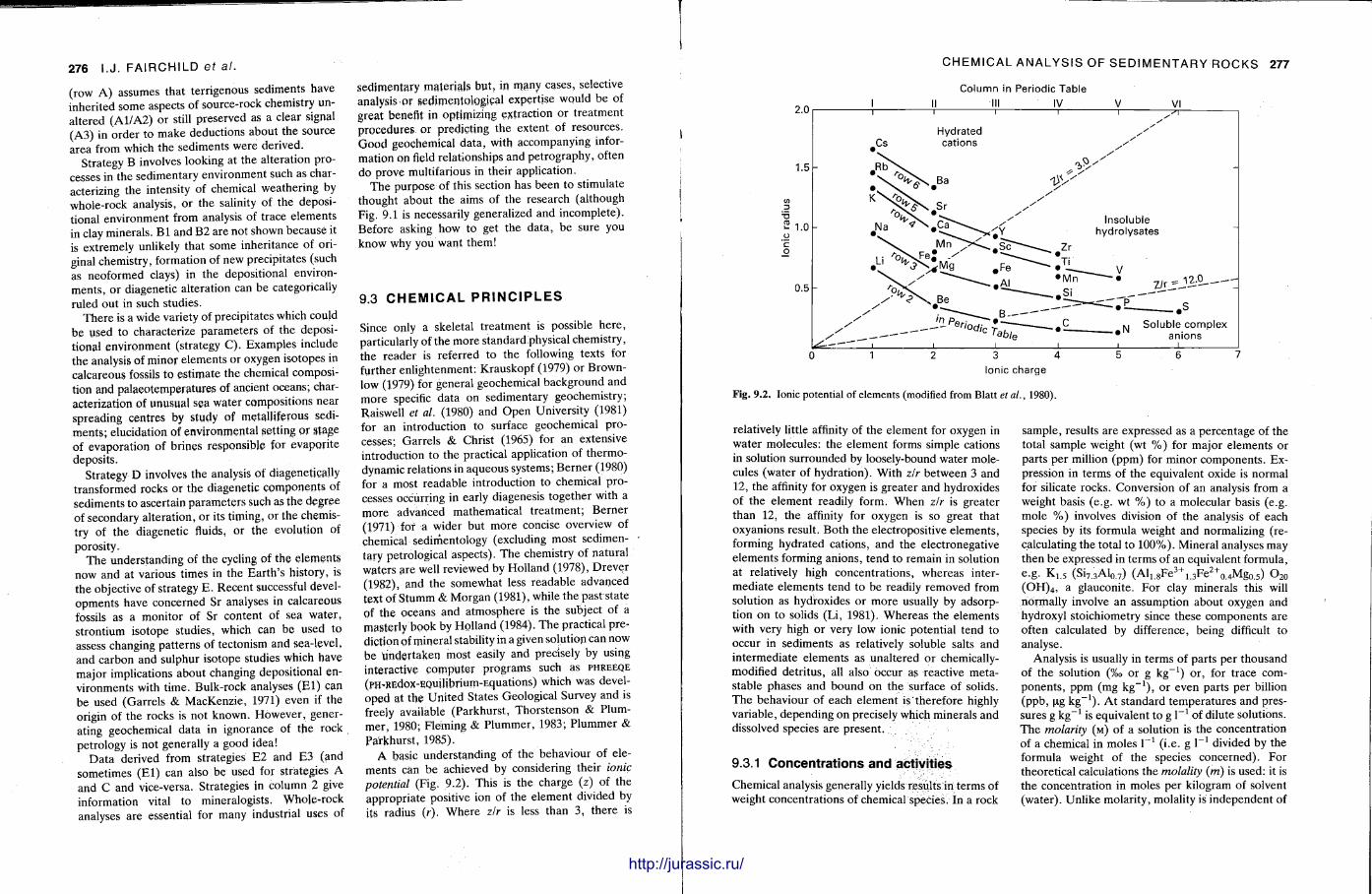
276 I.J. FAIRCHILD ef al.
(row A ) assumes that terr igenous sediments have inherited some aspects of source-rock chemistry unaltered (A1/A2) or still preserved as a clear signal (A3) in order to m a k e deductions about the source area from which the sediments were derived.
Strategy B involves looking at the alteration processes in the sedimentary environment such as characterizing the intensity of chemical weathering by whole-rock analysis, o r the salinity of the depositional environment from analysis of trace elements in clay minerals. B l and B2 are not shown because it is extremely unlikely that some inheri tance of original chemistry, formation of new precipitates (such as neoformed clays) in the depositional environments , or diagenetic alteration can be categorically ruled out in such studies.
There is a wide variety of precipitates which could be used to characterize parameters of the depositional environment (strategy C) . Examples include the analysis of minor e lements or oxygen isotopes in calcareous fossils to est imate the chemical composition and palaeotemperatures of ancient oceans; characterization of unusual sea water compositions near spreading centres by study of metalliferous sediments ; elucidation of environmental setting o r stage of evaporat ion of brines responsible for evapori te deposits.
Strategy D involves the analysis of diagenetically transformed rocks or the diagenetic components of sediments to ascertain parameters such as the degree of secondary al terat ion, or its t iming, or the chemistry of the diagenetic fluids, or the evolution of porosity.
The understanding of the cycling of the elements now and at various t imes in the Ear th ' s history, is the objective of strategy E . Recent successful developments have concerned Sr analyses in calcareous fossils as a monitor of Sr content of sea water , s trontium isotope studies, which can be used to assess changing pat terns of tectonism and sea-level, and carbon and sulphur isotope studies which have major implications about changing depositional environments with t ime. Bulk-rock analyses ( E l ) can be used (Garrels & MacKenzie , 1971) even if the origin of the rocks is not known. However , generating geochemical da ta in ignorance of the rock petrology is not generally a good idea!
Da ta derived from strategies E 2 and E 3 (and sometimes ( E l ) can also be used for strategies A and C and vice-versa. Strategies in column 2 give information vital to mineralogists. Whole-rock analyses are essential for many industrial uses of
sedimentary materials bu t , in many cases, selective analysis or sedimentologieal expertise wquld be of great benefit in optimizing extraction or t rea tment procedures or predicting the extent of resources. G o o d geochemical da ta , with accompanying information on field relationships and petrography, often do prove multifarious in their application.
T h e purpose of this section has been to stimulate thought about the aims of the research (although Fig. 9.1 is necessarily generalized and incomplete) . Before asking how to get the da ta , be sure you know why you want them!
9.3 C H E M I C A L P R I N C I P L E S
Since only a skeletal t rea tment is possible here , particularly of the more standard physical chemistry, the reader is referred to the following texts for further enl ightenment: Krauskopf (1979) or Brown-low (1979) for general geochemical background and more specific da ta on sedimentary geochemistry; Raiswell et al. (1980) and Open University (1981) for an introduction to surface geochemical processes; Garre ls & Christ (1965) for an extensive introduction to the practical application of thermodynamic relations in aqueous systems; Berner (1980) for a most readable introduction t o chemical processes occurring in early diagenesis together with a more advanced mathematical t rea tment ; Berner (1971) for a wider but more concise overview of chemical sedimentology (excluding most sedimentary petrological aspects). T h e chemistry of natural waters are well reviewed by Holland (1978), Drever (1982), and the somewhat less readable advanced text of S tumm & Morgan (1981), while the pas t s t a t e of the oceans and a tmosphere is the subject of a masterly book by Holland (1984). The practical prediction of mineral stability in a given solution can now be under taken most easily and precisely by using interactive computer programs such as phreeqe (pH-REdox-EQuilibrium-Equations) which was developed at the Uni ted States Geological Survey and is freely available (Parkhurst , Thors tenson & Plum-mer , 1980; Fleming & Plummer , 1983; P lummer & Parkhurst , 1985).
A basic understanding of the behaviour of elements can be achieved by considering their ionic potential (Fig. 9.2). This is the charge (z) of the appropria te positive ion of the e lement divided by its radius (r) . Where zlr is less than 3 , there is
CHEMICAL ANALYSIS OF SEDIMENTARY ROCKS 277
Soluble complex anions
i 3 4
Ionic charge
Fig. 9.2. Ionic potential of elements (modified from Blatt et al., 1980).
relatively little affinity of the e lement for oxygen in water molecules: the e lement forms simple cations in solution surrounded by loosely-bound water molecules (water of hydrat ion) . With zlr between 3 and 12, the affinity for oxygen is greater and hydroxides of the e lement readily form. When zlr is greater than 12, the affinity for oxygen is so great that oxyanions result. Bo th the electropositive e lements , forming hydrated cations, and the electronegative elements forming anions, tend to remain in solution at relatively high concentrat ions, whereas intermedia te e lements tend to be readily removed from solution as hydroxides or more usually by adsorption on to solids (Li, 1981). Whereas the elements with very high or very low ionic potential tend to occur in sediments as relatively soluble salts and intermediate e lements as unaltered or chemically-modified detri tus, all also occur as reactive meta-stable phases and bound on the surface of solids. The behaviour of each element is therefore highly variable, depending on precisely which minerals and dissolved species are present .
9.3.1 Concentrat ions and activit ies
Chemical analysis generally yields results in terms of weight concentrat ions of chemical species. In a rock
sample, results are expressed as a percentage of the total sample weight (wt % ) for major elements or parts per million (ppm) for minor components . Expression in terms of the equivalent oxide is normal for silicate rocks. Conversion of an analysis from a weight basis (e.g. wt % ) to a molecular basis (e.g. mole % ) involves division of the analysis of each species by its formula weight and normalizing (recalculating the total to 100%). Mineral analyses may then be expressed in terms of an equivalent formula, e.g. Ki 5 ( S i 7 : i A l „ / ) ( A l 1 . 8 F e 3 +
1 . 3 F e 2 + o . 4 M g 0 . 5 ) O 2 0
( O H ) 4 , a glauconite. For clay minerals this will normally involve an assumption about oxygen and hydroxyl stoichiometry since these components are often calculated by difference, being difficult to analyse.
Analysis is usually in terms of parts per thousand of the solution ( % o or g k g - 1 ) or , for trace components , ppm (mg k g - 1 ) , or even parts per billion (ppb, ug k g - 1 ) . At standard temperatures and pressures g k g - 1 is equivalent to g l - 1 of dilute solutions. The molarity ( M ) of a solution is the concentration of a chemical in moles F" 1 ( i .e . g 1 _ 1 divided by the formula weight of the species concerned) . For theoretical calculations the molality (m) is used: it is the concentrat ion in moles per kilogram of solvent (water) . Unlike molarity, molality is independent of
Column in Periodic Table IV
http://jurassic.ru/
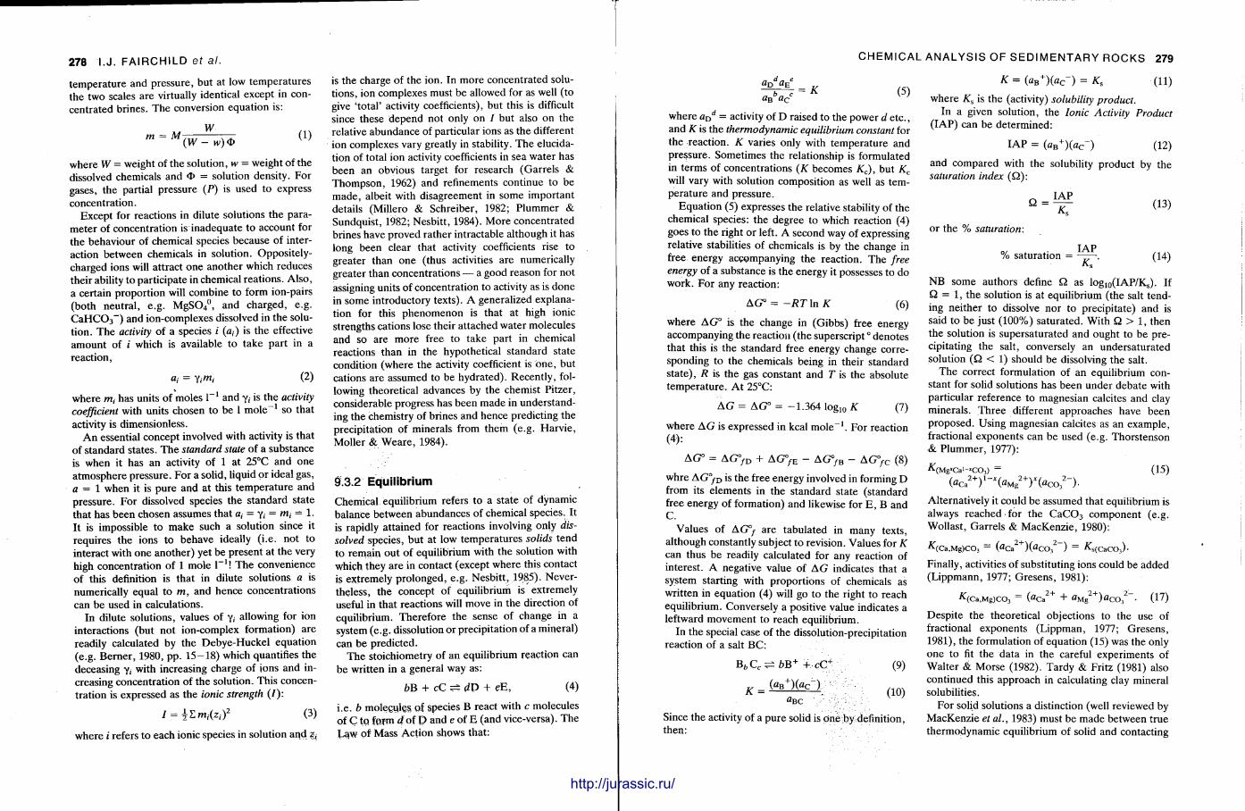
278 I.J. FAIRCHILD e t a l .
t empera ture and pressure, but at low tempera tures the two scales are virtually identical except in concentrated brines. T h e conversion equation is:
where W = weight of the solution, w = weight of the dissolved chemicals and <I> = solution density. For gases, the partial pressure (P) is used to express concentrat ion.
Except for reactions in dilute solutions the parameter of concentrat ion is~ inadequate to account for the behaviour of chemical species because of interaction between chemicals in solution. Oppositely-charged ions will attract one another which reduces their ability to part icipate in chemical reat ions. Also , a certain proport ion will combine to form ion-pairs (both neutra l , e.g. M g S O 4
0 , and charged, e.g. C a H C 0 3 ~ ) and ion-complexes dissolved in the solut ion. T h e activity of a species i ( a ; ) is the effective amoun t of / which is available to t ake par t in a react ion,
a, = Y,m, (2)
where m, has units of moles l - 1 and y,- is the activity coefficient with units chosen to be 1 m o l e - 1 so that activity is dimensionless.
A n essential concept involved with activity is that of s tandard states. T h e standard state of a substance is when it has an activity of 1 at 25°C and one a tmosphere pressure . For a solid, liquid or ideal gas, a = 1 when it is pure and at this t empera ture and pressure . For dissolved species the s tandard state that has been chosen assumes that «,• = y, = = 1. It is impossible to make such a solution since it requires the ions to behave ideally ( i .e . not to interact with o n e ano ther ) yet be present a t the very high concentrat ion of 1 mole T h e convenience of this definition is that in dilute solutions a is numerically equal to m, and hence concentrat ions can be used in calculations.
In dilute solutions, values of y,- allowing for ion interactions (but not ion-complex formation) are readily calculated by the Debye-Huckel equat ion (e .g. Berner , 1980, p p . 15—18) which quantifies the deceasing y, with increasing charge of ions and increasing concentrat ion of the solution. This concentration is expressed as the ionic strength (I):
7 = | S m , ( z , ) 2 (3)
where i refers to each ionic species in solution and
is the charge of the ion. In more concentrated solutions, ion complexes must be allowed for as well ( to give ' total ' activity coefficients), but this is difficult since these depend not only on / but also on the relative abundance of particular ions as the different ion complexes vary greatly in stability. The elucidation of total ion activity coefficients in sea water has been an obvious target for research (Garrels & Thompson , 1962) and refinements cont inue to be made , albeit with disagreement in some impor tant details (Millero & Schreiber, 1982; P lummer & Sundquist , 1982; Nesbitt , 1984). More concentrated brines have proved rather intractable al though it has long been clear that activity coefficients rise to greater than one (thus activities are numerically greater than concentrat ions — a good reason for not assigning units of concentrat ion to activity as is done in some introductory texts). A generalized explanation for this phenomenon is that at high ionic strengths cations lose their at tached water molecules and so are more free to take part in chemical reactions than in the hypothetical s tandard state condition (where the activity coefficient is one , but cations are assumed to be hydrated) . Recent ly , following theoretical advances by the chemist Pitzer, considerable progress has been m a d e in unders tanding the chemistry of brines and hence predicting the precipitation of minerals from them (e.g. Harv ie , Moller & W e a r e , 1984).
9.3.2 Equi l ibr ium
Chemical equilibrium refers to a state of dynamic balance between abundances of chemical species. It is rapidly attained for reactions involving only dissolved species, but at low tempera tures solids tend to remain out of equilibrium with the solution with which they are in contact (except where this contact is extremely prolonged, e.g. Nesbitt , 1985). Nevertheless, the concept of equilibrium is extremely useful in that reactions will move in the direction of equilibrium. Therefore the sense of change in a system (e.g. dissolution or precipitation of a mineral) can be predicted.
T h e stoichiometry of an equilibrium reaction can be written in a general way as:
bB + cC =± dD + eE, (4)
i.e. b molecules pf species B react with c molecules of C tQ ferm dof D and e of E (and vice-versa). The Law of Mass Act ion shows that:
CHEMICAL ANALYSIS OF SEDIMENTARY ROCKS 279
a p a t 6
= K (5)
where aD
d = activity of D raised to the power d e tc . , and K is the thermodynamic equilibrium constant for the reaction. K varies only with tempera ture and pressure. Sometimes the relationship is formulated in terms of concentrat ions (K becomes Kc), but Kc
will vary with solution composit ion as well as tempera ture and pressure.
Equat ion (5) expresses the relative stability of the chemical species: the degree to which reaction (4) goes to the right or left. A second way of expressing relative stabilities of chemicals is by the change in free energy accompanying the reaction. The free energy of a substance is the energy it possesses to do work. For any reaction:
AG° = -RT In K (6)
where AG" is the change in (Gibbs) free energy accompanying the reaction ( the superscript ° denotes that this is the standard free energy change corresponding to the chemicals being in their s tandard s ta te) , R is the gas constant and T is the absolute t empera ture . A t 25°C:
A G = AG° = - 1 . 3 6 4 l o g 1 0 K (V)
where A G is expressed in kcal mole l . For reaction (4):
AG" = A G ° / D + A G 7 E - A G ° / B - A G ° / C (8)
whre AG°fD is t he free energy involved in forming D from its e lements in the standard state (standard free energy of formation) and likewise for E , B and C.
Values of AG°/ are tabulated in many texts, al though constantly subject to revision. Values for K can thus b e readily calculated for any reaction of interest. A negative value of A G indicates that a system starting with proport ions of chemicals as written in equat ion (4) will go to the right to reach equilibrium. Conversely a positive value indicates a leftward movement to reach equilibrium.
In the special case of the dissolution-precipitation reaction of a salt BC:
B , , C , . b B + + cC~
K = ( * B + ) ( f i C - )
(9)
(10)
Since the activity of a pure solid is one by definition, then:
K = (aB
+)(ac-) = Ks (11)
where Ks is the (activity) solubility product. In a given solution, the Ionic Activity Product
( IAP) can be determined:
I A P = (aB
+)(ac-) (12)
and compared with the solubility product by the saturation index (Q) :
Q = I A P
(13)
or the % saturation:
I A P % saturation = t L £ r ~ . (14)
N B some authors define Q as l o g 1 0 ( I A P / K s ) . If Q = 1, the solution is at equilibrium (the salt tending nei ther to dissolve nor to precipitate) and is said to be just (100%) saturated. With Q > 1, then the solution is supersaturated and ought to b e pre cipitating the salt, conversely an undersaturated solution ( Q < 1) should be dissolving the salt.
The correct formulation of an equilibrium constant for solid solutions has been under deba te with particular reference to magnesian calcites and clay minerals. Th ree different approaches have been proposed. Using magnesian calcites as an example, fractional exponents can b e used (e .g. Thors tenson & Plummer , 1977):
K, ( M g ^ C a ' - ' C O j ) —
( a C a
2 y - * ( a M g
2 + y ( a C O i
2 - ) -
(15)
Alternatively it could be assumed that equilibrium is always reached for the C a C 0 3 component (e.g. Wollast , Garre ls & MacKenzie , 1980):
^ ( C a , M g ) C 0 3 = ( « C a 2 + ) ( f l C O , 2 ) = ^ s ( C a C O , ) -
Finally, activities of substituting ions could be added (Lippmann, 1977; Gresens , 1981):
^ ( C a , M g ) C 0 3 = ° M g > c o 3
2 - - (17)
Despi te the theoretical objections to the use of fractional exponents (Lippman, 1977; Gresens , 1981), the formulation of equat ion (15) was the only one to fit the data in the careful experiments of Walter & Morse (1982). Tardy & Fritz (1981) also continued this approach in calculating clay mineral solubilities.
For solid solutions a distinction (well reviewed by MacKenzie et al., 1983) must be made between true thermodynamic equilibrium of solid and contacting
http://jurassic.ru/
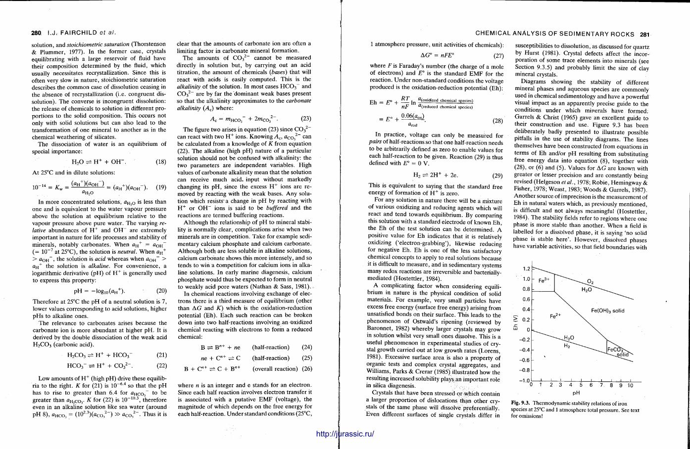
280. I.J. FAIRCHILD et al:
solution, and stoichiometric saturation (Thorstenson & Plummer , 1977). In the former case, crystals equilibrating with a large reservoir of fluid have their composition determined by the fluid, which usually necessitates recrystallization. Since this is often very slow in na ture , stoichiometric saturation describes the common case of dissolution ceasing in the absence of recrystallization (i .e. congruent dissolution). T h e converse is incongruent dissolution: the release of chemicals to solution in different proport ions to the solid composit ion. This occurs not only with solid solutions but can also lead to the transformation of one mineral to another as in the chemical weathering of silicates.
T h e dissociation of water is an equilibrium of special importance:
H z O ^± H + + O H - . (18)
At 25°C and in dilute solutions:
1 0 - 1 . = K w = ( « H + X « O H - ) = ( a H + ) ( f l o i r ) . ( w )
In more concentrated solutions, a H , 0 is less than one and is equivalent to the water vapour pressure above the solution at equilibrium relative to the vapour pressure above pure water . T h e varying relative abundances of H + and O H ~ are extremely important in na ture for life processes and stability of minerals , notably carbonates . When aH
+ — aOH~ ( = 10~ 7 at 25°C), the solution is neutral. When a H
+
> A o h " , the solution is acid whereas when a O H ~ > a H
+ the solution is alkaline. For convenience, a logarithmic derivative (pH) of H + is generally used to express this property:
p H = - l o g 1 0 ( f l H
+ ) . (20)
Therefore at 25°C the p H of a neutral solution is 7, lower values corresponding to acid solutions, higher pHs to alkaline ones.
The relevance to carbonates arises because the carbonate ion is more abundant at higher p H . It is derived by the double dissociation of the weak acid H 2 C 0 3 (carbonic acid).
H 2 C 0 3 ?± H + + H C C V (21)
HCO-T ^ H + + C 0 3
2 " . (22)
Low amounts of H + ( h i g h p H ) drive these equilibria to the right. K for (21) is 1 0 " 6 4 so that the p H has to rise to greater than 6.4 for aHCO~ to be greater than a H , c o 3 - K for (22) is 1 0 " 1 0 3 , therefore even in an alkaline solution like sea water (around p H 8) , flHco3 = (10 2 - 3 ) ( f l co , 2 - ) » " c o , 2 " - Thus it is
clear that the amounts of carbonate ion are often a limiting factor in carbonate mineral formation.
The amounts of C 0 3
2 ~ cannot be measured directly in solution but , by carrying out an acid t i tration, the amount of chemicals (bases) that will react with acids is easily computed . This is the alkalinity of the solution. In most cases H C 0 3 ~ and C 0 3
2 ~ are by far the dominant weak bases present so that the alkalinity approximates to the carbonate alkalinity (Ac) where :
A c = mHCO~ + 2 m C o 3
2 " - (23)
The figure two arises in equat ion (23) since C 0 3
2 ~ can react with two Ff + ions. Knowing Ac, aco
2~ can be calculated from a knowledge of K from equat ion (22). The alkaline (high p H ) nature of a particular solution should not be confused with alkalinity: the two parameters are independent variables. High values of carbonate alkalinity mean that the solution can receive much acid, input without markedly changing its p H , since the excess H + ions are removed by reacting with the weak bases. Any solution which resists" a change in p H by reacting with H + or O H ~ ions is said to be buffered and the reactions are te rmed buffering reactions.
Al though the relationship of p H to mineral stability is normally clear, complications arise when two minerals a re in competi t ion. Take for example sedimentary calcium phosphate and calcium carbonate . Al though both are less soluble in alkaline solutions, calcium carbonate shows this more intensely, and so tends to win a Competition for calcium ions in alkaline solutions. In early marine diagenesis, calcium phosphate would thus be expected to form in neutral to weakly acid pore waters (Nathan & Sass, 1981).
In chemical reactions involving exchange of electrons there is a third measure of equilibrium (other than A G and K) which is the oxidation-reduction potential (Eh) . Each such reaction can be broken down into two half-reactions involving a n Oxidized chemical reacting with electrons to form a reduced chemical:
B ^ B " + + ne (half-reaction) (24)
ne + Cn+ ^± C (half-reaction) (25)
B + C + ^± C + B " + (overall reaction) (26)
where n is an integer and e stands for an electron. Since each half reaction involves electron transfer it is associated with a putative E M F (voltage), the magni tude of which depends on the free energy for each half-reaction. Unde r s tandard conditions (25°C,
CHEMICAL ANALYSIS OF SEDIMENTARY ROCKS 281
1 a tmosphere pressure , unit activities of chemicals):
AG" = nFE° (27)
where F is Faraday 's number (the charge of a mole of electrons) and E" is the s tandard E M F for the reaction. U n d e r non-s tandard condit ions the voltage produced is the oxidation-reduction potential (Eh) :
2-^ 7?7" " ( o x i d i z e d c h e m i c a l s p e c i e s ) En = IL + — ~ In 7; HP " ( r e d u c e d c h e m i c a l s p e c i e s )
= E> + ̂ 4 (28) " r e d
In practice, voltage can only be measured for pairs of half-reactions so that one half-reaction needs to be arbitrarily defined as zero to enable values for each half-reaction to be given. React ion (29) is thus defined with E° = 0 V .
H 2 ^± 2 H + + 2e . (29)
This is equivalent to saying that the standard free energy of formation of H + is zero .
For any solution in na ture the re will b e a mixture of various oxidizing and reducing agents which will react and tend towards equilibrium. By comparing this solution with a s tandard electrode of known E h , the E h of the test solution can be determined. A positive value for E h indicates that it is relatively oxidizing ( 'electron-grabbing') , likewise reducing for negative Eh . Eh is one of the less satisfactory chemical concepts to apply to real solutions because it is difficult to measure , and in sedimentary systems many redox reactions are irreversible and bacterially-mediated (Hostet t ler , 1984).
A complicating factor when considering equilibr ium in nature is the physical condition of solid materials . For example , very small particles have excess free energy (surface free energy) arising from unsatisfied bonds on their surface. This leads to the phenomenon of Ostwald 's ripening (reviewed by Baronnet , 1982) whereby larger crystals may grow in solution whilst very small ones dissolve. This is a useful phenomenon in experimental studies of crystal growth carried out at low growth rates (Lorens , 1981). Excessive surface area is also a property of organic tests and complex crystal aggregates, and Williams, Parks & Crerar (1985) illustrated how the resulting increased solubility plays an important role in silica diagenesis.
Crystals that have been stressed or which contain a larger proport ion of dislocations than o ther crystals of the same phase will dissolve preferentially. Even different surfaces of single crystals differ in
susceptibilities to dissolution, as discussed for quartz by Hurs t (1981). Crystal defects affect the incorporat ion of some trace elements into minerals (see Section 9.3.5) and probably limit the size of clay mineral crystals.
Diagrams showing the stability of different mineral phases and aqueous species are commonly used in chemical sedimentology and have a powerful visual impact as an apparent ly precise guide to the conditions under which minerals have formed. Garrels & Christ (1965) gave an excellent guide to their construction arid use. Figure 9.3 has been deliberately badly presented to illustrate possible pitfalls in the use of stability diagrams. T h e lines themselves have been constructed from equations in te rms of E h and/or p H resulting from substituting free energy data into equat ion (8), together with (28), or (6) and (5). Values for A G are known with greater or lesser precision and are constantly being revised (Helgeson etal., 1978; Robie , Hemingway & Fisher, 1978; Weas t , 1983; Woods & Garre ls , 1987). Ano the r source of imprecision is the measurement of E h in natural waters which, as previously mentioned, is difficult and not always meaningful (Hostet t ler , 1984). T h e stability fields refer to regions where one phase is more stable than another . When a field is labelled for a dissolved phase , it is saying 'no solid phase is stable here ' . However , dissolved phases have variable activities, so that field boundaries with
pH
Fig. 9.3. Thermodynamic stability relations of iron species at 25°C and 1 atmosphere total pressure. See text for omissions!
http://jurassic.ru/
282 I.J. FAIRCHILD ef al.
solids depend on the choice of activity. In Fig. 9 .3 , the boundary between the F e 2 + and F e ( O H ) 3 fields is actually drawn in assuming aFe
2+ = 1 ( T 3 at the boundary , lower values for the activity would correspond to moving the line parallel to itself to the upper right. T h e caption to Fig. 9.3 should state: activities of F e 2 + and F e 3 + at field boundar ies are 1CT 3. Choosing an appropr ia te value for the limiting activity of a dissolved phase requires some geological judgement . For example , Curtis & Spears (1968) decided that since aFe
2+ < 1 0 " 6 in sea water then A F e
2 + = 10~ 6 would be an appropria te boundary condition for the F e 2 + field in a diagram expressing relationships in sea water , whereas in pore waters aFe
2+ = 10~ 3 would be apposite since activities of ferrous iron range up to this value there . A n o t h e r problem with Fig. 9.3 is that in o rde r to construct a field boundary for F e C 0 3 you need to know the total activity of the dissolved carboxy species (H 2 CG- 3 , HCO3" and CO3 2 "); the caption for Fig. 9.3 should have stated that their total activity was 1 0 - 2 in this case. Some fields are missing in Fig. 9.3: for example F e ( O H ) 2 + has a stability field between F e 3 + and F e ( O H ) 3 (e.g. Garrels & Christ , 1965, fig. 7—14). Thus one must be certain that relevant equilibria have not been forgotten. The diagram also implicitly assumes that activities of H S - are negligible, otherwise pyrite would have a stability field of substantial size. Silicates such as glauconite and berthier ine must also not be forgotten (Maynard , 1986). Finally, it would be more informative to plot E h against activity of H C 0 3 ~ or HS~ because these species vary much more than p H in practice (Curtis & Spears , 1968). A series of diagrams is needed to show the complete picture of the system.
Good examples of the utility of stability diagrams in diagenetic studies a re given by Davies et al. (1979), Hu tcheon (1981) and Curtis (1983).
When considering systems far removed from their s tandard s ta te , for example during burial diagenesis, the effects of t empera ture , pressure and salinity variations must be carefully considered. T a k e for example the relative stability of carbonate minerals and silica. Apparen t alternating silica-carbonate replacements have been explained simply in te rms of p H variations (Walker , 1962), but the solubility of silica shows little variation with p H until p H s of 9 o r more . Actually during steady burial, t empera ture (T) pressure ( F ) , p H and salinity (5 ) will probably all rise. For calcite the effects of T and p H are to decrease solubility, whereas P (with constant P c o 2 ) and 5 increase solubility. For quar tz , T, P and p H all
increase solubility, but S reduces it because of the reduct ion in a H , o which destabilizes hydrated silica in solution (Fournier , 1983). These concepts can be applied to permeable rocks in which convective flow is occurring (Wood , 1986) and indicate that quartz and carbonates can be transferred from one part of the rock mass to ano ther , often moving in opposite directions and hence giving rise to replacive relationships.
9.3.3 Departures f rom equi l ibr ium
W h e r e sediments are out of equilibrium with their contained fluids, this relates either to kinetic controls ( the slowness of chemical reactions o r movement of chemicals) or to biological interference.
The most important kinetic control concerns the behaviour of crystal surfaces involved in dissolution or growth, especially the lat ter . T h e presence of abundan t early diagenetic minerals such as glauconite or carbonate fluorapatite only in slowly-deposited marine calcareous sediments illustrates the kinetic control on crystal growth. Conversely the fact that slowly-deposited detrital sediments exist at all attests to the incomplete dissolution of mineral grains in undersatura ted waters .
Crystal growth in a clean, supersaturated solution is initially limited by a stage of nucleation, since nuclei below a certain critical size have excess free energy and are thus unstable. However , in the sedimentary environment there will normally already be nuclei in the system which can be overgrown, even if nucleus and overgrowth are different minerals (epitaxial overgrowth) . W h e r e supersaturat ion is low [Q (equat ion 13) close to 1] the critical nucleus size is larger and the availability of nuclei could then be rate-limiting, but such conditions also lead to slow crystal growth anyway.
If surface reactions ra ther than movement of chemicals limit the growth rate of crystals, then the m o d e of growth would be expected to be by addition to growth spirals a round screw dislocations occurring on the crystal surface, ra ther than by the birth and spreading of two-dimensional layers (Sunagawa, 1982). If Q is close to 1, then:
R = K(Q - l ) 2 (30)
where R is the growth ra te , frequently expressed in terms of a radial increase in crystal size, and K is a constant . Often the real growth-limiting factor is adsorpt ion (see Section 9.2.4) of foreign ions on the surface of the crystal. In this case the above equa-
CHEMICAL ANALYSIS OF SEDIMENTARY ROCKS 283
tion would probably become (Berner , 1980, p . 105):
R = K(Q - 1)" (31)
where n > 1. For example , Mg-adsorption strongly inhibits calcite growth, and adsorbed humic and fulvic acids and P 0 4
3 ~ inhibit the growth of aragonite (Berner et al., 1978). T h e importance of Mg as an inhibitor lies in its abundance in natural waters . Experimental studies (Meyer , 1984) on calcite growth have shown that numerous inorganic and organic species are more effective inhibitors, with F e 2 + being so by four orders of magni tude. Adsorpt ion phenomena are also important in controlling crystal habit (Boistelle, 1982).
For dissolution, we have:
R = K(l - Q ) " (cf. 31). (32)
where R refers to the dissolution ra te . Very slow dissolution rates caused by ion-adsorption are common: for example the dissolution of calcite and aragonite shells in undersa tura ted sea water where n = 4—5 (Keir, 1980), the reaction being limited by adsorption of P 0 4
3 _ . However , inhibition of dissolution of calcium carbonate by organic materials is generally related to physical covering, ra ther than adsorption phenomena (Morse , 1983).
Berner (1978a, 1980) has shown that where dissolution is controlled by surface reactions, the crystals have angular outlines with crystallographically-controlled etch pits: such surface-reaction control is normal in soils and nearly all surface waters .
Unde r some circumstances the rate of crystal growth or dissolution is controlled by the rate of movement of chemicals in solution rather than by reactions taking place on the crystal surface. This only seems feasible within pore waters and where precipitation or dissolution is unusually rapid (implying great supersaturat ion or undersa tura t ion) . Movement of chemicals in general may be by advec-tion (movement under forces, e.g. groundwater flow or the relative movement of grains and pore fluid due to compact ion) , dispersal by burrowing organisms or turbulence, or by molecular diffusion. The existence of appropr ia te concentrat ion gradients in solutions away from sites of, for example, manganese oxide or iron sulphide precipitation in Recent sediments demonst ra tes the importance of the transport-control mechanism. Growing crystals in these circumstances may be restricted t o a very fine crystal size, or show dendrit ic or spherulitic morphologies (Rodriguez-Clemente , 1982; Sunagawa, 1982); dissolving crystals will exhibit smoothly-rounded out
lines (Berner , 1978a, 1980). The existence of specifically di / j faHow -control led growth in sediments and sedimentary rocks is demonstra ted by Liese-gang ring phenomena , such as iron oxide bands formed during weather ing, or concentric mineralogical banding in concretions (De Celles & Gutschick, 1983). This arises where inter-diffusion of two species has led to precipitation of material at episodically-shifting sites.
The magni tude of a diffusional flux is given by Fick's first law of diffusion. It relates the mass of chemical component i t ransported per unit area per unit t ime (J) to its concentrat ion gradient (dCldx) across distance x:
where D,- is the diffusion coefficient, specific to the chemical component i (typically around 10~ 5 c m 2
s _ 1 for salts in water at 25°C). In a sediment , diffusion is slowed because of the effective increase in path length caused by the obstructions represented by the sediment grains. Thus the effective diffusion coefficient is smaller by a factor relating to the sediment porosity (e.g. <j>2 where (j) is the fractional porosity, Le rman , 1979). The re is also some variation of D, with salinity of a solution (e.g. Lerman , 1979, p . 81). Sometimes corrections are necessary to allow for ion-pairing effects (Mangelsdorf & Sayles, 1982). T h e behaviour of the diffusion gradient with t ime is covered by Fick's second law (e.g. Berner , 1980, pp . 32—33); diffusion acts to reduce the concentrat ion gradients but , if it is allowed to do so, the flux necessarily diminishes.
Enhanced movement of chemicals, because of the presence of open burrows in a sediment , can be modelled in a similar way, using a biodiffusion coefficient or , if complete bioturbation occurs, then a 'box modelling' approach can be used (Berner , 1980, pp . 4 2 - 5 3 ) .
A n advective flux can be calculated as the product of the concentrat ion of the component (C) and the velocity of flow (U),
J = CU. (34)
It is often useful to compare the effectiveness of diffusion with that of advective flow. If we imagine a situation where a diffusive flux in one direction is balanced by an advective flux in the other direction, then:
-Di^f- + CU = 0. (35)
http://jurassic.ru/
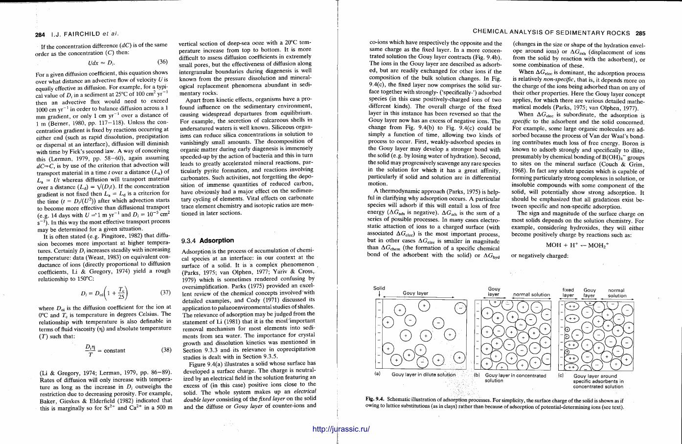
284 I.J. FAIRCHILD et al.
If the concentrat ion difference (dC) is of the same order as the concentrat ion (C) then:
Udx = Dj. (36)
For a given diffusion coefficient, this equation shows over what distance an advective flow of velocity U is equally effective as diffusion. For example, for a typical value of D, in a sediment at 25°C of 100 c m 2 y r _ 1
then an advective flux would need to exceed 1000 cm y r - 1 in order to balance diffusion across a 1 mm gradient, or only 1 cm y r _ 1 over a distance of 1 m (Berner , 1980, pp . 117 -118) . Unless the concentration gradient is fixed by reactions occurring at either end (such as rapid dissolution, precipitation or dispersal at an interface), diffusion will diminish with t ime by Fick's second law. A way of conceiving this (Lerman, 1979, pp . 58—60), again assuming dC~C, is by use of the criterion that advection will t ransport material in a t ime t over a distance ( L a ) of L a = Ut whereas diffusion will t ransport material over a distance ( L d ) = y/(D,-t). If the concentrat ion gradient is not fixed then L a = L d is a criterion for the t ime (r = D, / ({ / 2 ) ) after which advection starts to become m o r e effective than diffusional t ransport (e.g. 14 days with ( / = ' l m y r _ 1 and D ; = 1 0 " 5 c m 2
s _ 1 ) . In this way the most effective t ransport process may be de termined for a given situation.
It is often stated (e.g. Pingitore, 1982) that diffusion becomes more important at higher temperatures . Certainly D, increases steadily with increasing tempera ture : data (Weast , 1983) on equivalent conductance of ions (directly proport ional to diffusion coefficients, Li & Gregory , 1974) yield a rough relationship to 150°C:
A = Z > o i ( l + (37)
where Doj is the diffusion coefficient for the ion at 0°C and Tc is t empera ture in degrees Celsius. The relationship with t empera ture is also definable in terms of fluid viscosity (T)) and absolute t empera tu re ( 7 / ) such that:
—^r = constant (38)
(Li & Gregory, 1974; Le rman , 1979, pp . 8 6 - 8 9 ) . Ra tes of diffusion will only increase with temperature as long as the increase in Dt outweighs the restriction due to decreasing porosity. For example , Baker , Gieskes & Elderfield (1982) indicated that this is marginally so for S r 2 + and C a 2 + in a 500 m
vertical section of deep-sea ooze with a 20°C temperature increase from top to bo t tom. It is more difficult to assess diffusion coefficients in extremely small pores , but the effectiveness of diffusion along intergranular boundaries during diagenesis is well known from the pressure dissolution and mineralogical replacement phenomena abundant in sedimentary rocks:
Apar t from kinetic effects, organisms have a profound influence on the sedimentary environment , causing widespread depar tures from equil ibrium. For example , the secretion of calcareous shells in undersatured waters is well known. Siliceous organisms can reduce silica concentrat ions in solution to vanishingly small amounts . T h e decomposit ion of organic mat ter during early diagenesis is immensely speeded-up by the action of bacteria and this in turn leads to greatly accelerated mineral reactions, particularly pyrite formation, and reactions involving carbonates . Such activities, not forgetting the deposition of immense quantit ies of reduced carbon, have obviously had a major effect on the sedimentary cycling of e lements . Vital effects on carbonate trace element chemistry and isotopic ratios are mentioned in later sections.
9.3.4 Adsorpt ion
Adsorpt ion is the process of accumulation of chemical species at an interface: in our context at the surface of a solid. It is a complex phenomenon (Parks , 1975; van Olphen , 1977; Yariv & Cross , 1979) which is sometimes rendered confusing by oversimplification. Parks (1975) provided an excellent review of the chemical concepts involved'with detailed examples , and Cody (1971) discussed its application to palaeoenvironmental studies of shales. T h e relevance of adsorption may be judged from the s ta tement of Li (1981) that it is the most important removal mechanism for most e lements into sediments from sea water . The importance for crystal growth and dissolution kinetics was ment ioned in Section 9.3.3 and its relevance in coprecipitation studies is dealt with in Section 9.3.5.
Figure 9.4(a) illustrates a solid whose surface has developed a surface charge. The charge is neutralized by an electrical field in the solution featuring an excess of (in this case) positive ions close to the solid. The whole system makes up an electrical double layer consisting of the fixed layer on the solid and the diffuse o r Gouy layer of counter-ions and
CHEMICAL ANALYSIS OF SEDIMENTARY ROCKS 285
co-ions which have respectively the opposi te and the same charge as the fixed layer. In a more concentrated solution the Gouy layer contracts (Fig. 9.4b). The ions in the Gouy layer are described as adsorbed, but are readily exchanged for other ions if the composition of the bulk solution changes. In Fig. 9.4(c), the fixed layer now comprises the solid surface together with strongly- ('specifically-') adsorbed species (in this case positively-charged ions of two different kinds). The overall charge of the fixed layer in this instance has been reversed so that the Gouy layer now has an excess of negative ions. The change from Fig. 9.4(b) to Fig. 9.4(c) could be simply a function of t ime, allowing two kinds of process to occur. First, weakly-adsorbed species in t he Gouy layer may develop a stronger bond with the solid (e.g. by losing water of hydrat ion) . Second, the solid may progressively scavenge any rare species in the solution for which it has a great affinity, particularly if solid and solution are in differential mot ion.
A thermodynamic approach (Parks, 1975) is helpful in clarifying why adsorption occurs. A particular species will adsorb if this will entail a loss of free energy ( A G a d s is negative). A G a d s is the sum of a series of possible processes. In many cases electrostatic attaction of ions to a charged surface (with associated A G e i e c ) is the most important process, but in o ther cases AG eiec is smaller in magni tude than A G c h e m ( the formation of a specific chemical bond of t he adsorbent with t he solid) or A G h y d
(changes in the size or shape of the hydration envelope around ions) or A G r x h (displacement of ions from the solid by reaction with the adsorbent ) , or some combination of these.
When A G e i e c is dominant , the adsorption process is relatively non-specific, that is, it depends more on the charge of t he ions being adsorbed than on any of their o ther propert ies . H e r e the Gouy layer concept applies, for which there are various detailed mathematical models (Parks , 1975; van Olphen, 1977).
W h e n AGeiec <s subordina te , the adsorption is specific to the adsorbent and the solid concerned. For example , some large organic molecules are adsorbed because the process of Van der Waal 's bonding contr ibutes much loss of free energy. Boron is known to adsorb strongly and specifically to illite, presumably by chemical bonding of B ( O H ) 4 ~ groups to sites on the mineral surface (Couch & Gr im, 1968). In fact any solute species which is capable of forming particularly strong complexes in solution, or insoluble compounds with some component of the solid, will potentially show strong adsorption. It should be emphasized tha t all gradations exist between specific and non-specific adsorption.
T h e sign and magni tude of t he surface charge on most solids depends on the solution chemistry. For example , considering hydroxides, they will either become positively charge by reactions such as:
M O H + H + — M O H 2
+
or negatively charged:
Solid Gouy layer
0 © © 0 O 0 0 0 0 o°0 0:§
(a) Gouy layer in dilute solution
Gouy layer normal solution
m m
(b) Gouy layer in concentrated solution
fixed Gouy layer layer
normal solution
Gouy layer around specific adsorbents in concentrated solution
Fig. 9.4. Schematic illustration of adsorption processes. For simplicity, the surface charge of the solid is shown as if owing to lattice substitutions (as in clays) rather than because of adsorption of potential-determining ions (see text).
http://jurassic.ru/
286 I.J. FAIRCHILD et al. (proport ional to the number of sites occupied by the adsorbent) . This logic (e.g. Yariv & Cross, 1979, pp. 120-123) leads to a form of equat ion known as the Langmuir isotherm:
Q d — abC,,
1 + ( a C s o l ) ( 3 9 )
where C a d is the concentrat ion of adsorbed species (per unit mass of solid), C s o l is the concentrat ion in solution and a and b are constants , b being a measure of the total number of adsorption sites. The assumptions involved are probably not valid in concentrated solution where , for example , new adsorption sites on clays may become available (Cody, 1971).
W h e r e adsorption sites are not saturated, an empirical equat ion ( the Freundlich isotherm) often fits:
Cad = K(Csolf" (40)
where n > 1 and K is a constant . A t low concentrat ions, a simplified form is often applicable:
Q d = KCsol. (41)
Adsorbed ions are more or less readily exchangeable. The total amount of exchangeable cations (cation-exchange capacity, C E C ) is measured in terms of milliequivalents (millimoles times charge) of exchangeable cations per 100 g of dry substance, and is highly dependen t on its specific surface area. Typical values range from 100 to 300 for organic mat ter and zeolites, through 70—80 for smectites, 10—40 for illites and 3 - 1 5 for kaolinite (Le rman , 1979).
Ion-exchange takes place readily when A G e i e c
forms a large propor t ion of A G a d s . Wi th Gouy-layer type adsorpt ion all ions of the same charge 'are competing for the adsorption sites. If AG e i e c were overridingly important then the relative concentrations (strictly activities) of the adsorbed ions would be equal to their relative concentrat ions (or activities) in the bulk solution. In practice this is not so and, using clays as an example , adsorpt ion affinity decreases with decreasing hydrated ion radius, for example from bot tom to top of columns I and II of the periodic table . This can be expressed in t e rms of an exchange reaction (between equally-charged ions, as the simplest example) :
A + + B a d ^ B + + A a (42)
for which the equilibrium constant (K not equal to one) is:
CHEMICAL ANALYSIS OF SEDIMENTARY ROCKS 287
K = ( « B + ) ( « A a d )
(f lA + ) ( « B a d ) ' (43)
Since activity coefficients for adsorbed ions are not readily est imated and often appear to be close to unity, mole fractions (x) are frequently used instead of activities of adsorbed species. If the system is noticeably non-ideal (for example when large variations in compositions are being considered) then mole fractions may still be used with a different (empirical) form of equat ion:
X A
Xft = K'
« B 4
(44)
where K' and p are constants for the pair of adsorbents considered (Lerman , 1979, p . 346).
Altervalent ion-exchange has been found to be an important mechanism in experiments on freshwater clays exposed to sea water (Sayles & Mangelsdorf, 1977, 1979). Equat ions (42) and (43) can be modified to model this process (e.g. Berner , 1980, p . 70) and carry the important implication that the less highly-charged ion will be preferentially adsorbed in solutions of progressively higher ionic strength because its activity coefficient in solution will fall more slowly. Exper iments on exposure of clays to sea water also show that C E C diminishes with t ime as K + becomes specifically sorbed on to degraded illites (Russell , 1970). Ion-exchange reactions and specific adsorption processes are also very important during weathering and burial diagenesis.
Li (1981) considered adsorption as a mechanism for controlling the ratios of concentrat ions of elements in oceanic pelagic sediments and in sea water by plotting these ratios against equilibrium constants for reactions involved in adsorption on O H sites on solids. (These equilibrium constants correlate fairly well with ionic potential . ) Most elements fall within a band on such plots, consistent with adsorption being a major control on their behaviour.
The complexing of trace metals to organic material can be extremely impor tant as a means of introducing elements to sediments even if later released by organic decay and fixed in other ways. Unfortunately the mechanisms of complexat ion (e.g. by specific adsorpt ion, or alternatively by chelation, i .e. bonded to O , N or S and lying centrally in ring structures) is not often known (Jackson, Jonasson & Skippen, 1978), especially in sea water: Chelation is well-known for example for V and Ni in petroleum and oil shales (e.g. Riley & Saxby, 1982). A number
of elements are found to correlate with organic carbon in black shales (e.g. M o , Ni, Cu , V, Co , U , Z n , H g and As in the study of Leventhal & Hoster-man , 1982) which is empirical evidence for the importance of the association of organic molecules and metals in sea water .
Nyffeler, Li & Santschi (1984) performed experiments on the rates of adsorption processes to test whether particles remained long enough in sea water to reach a state of equilibrium adsorption. Where particles only reside for a few days in the water column it seems that equilibration may not be complete and will certainly not be so for certain elements (Be , Mn , Co and Fe) . However , for several of these e lements , removal of adsorption on to manganese nodules will be continuously available. In principle, however , sedimentat ion rate and aspects of sedimentary environment (e .g. water dep th ) , even with constant water chemistry, are liable to affect the minor e lement (adsorbed species) composition of sediments. Variat ions in salinity or organic carbon flux to sediments will be major controls on trace element content .
When considering use of adsorbed trace elements to characterize the chemistry of depositional environments , specific adsorbents are required that will not readily be diagenetically-altered. Possible problems are inheri tance of trace elements in detrital phases , control of up take by several chemical parameters (e.g. p H , t empera ture and salinity), and variations in mineralogical abundances and surface propert ies even of individual minerals (Cody, 1971). Success only seems likely when making comparat ive studies, within a geological unit , using selective analyses, on a specific mineral species (see Section 9.8).
9.3.5 Lattice incorporat ion of trace elements
T h e object of studying trace elements in minerals is normally to constrain the chemistry of the precipitating solution, or to assess the degree of chemical exchange during diagenetic alterations (Brand & Veizer , 1980; Veizer, 1983). Usually interpretat ions are only possible when coprecipitation of the trace element by substitution for a host (carrier) ion of similar radius and electronegativity has occurred (Mclntyre , 1963). Ions occupying interstitial lattice positions may also be amenable to analysis and interpretation (Ishikawa & Ichikuni, 1984), although
M O H — M O " + H + .
Excess of H + ions, as in acid solutions, promotes a positive charge which decreases with increasing p H until a point of zero charge (pzc), specific for each substance, is reached, followed by the development of a negative charge at higher p H . Oxides behave in a similar way, since their surface oxygens become hydroxyl groups adjacent to aqueous solutions. Thus for oxides and hydroxides, H + determines the charge and hence the electric potential of the surface: it is the potential-determining ion (PDI ) . P D I s for salts such as C a C 0 3 are its constituent ions, positive charge being expected when ACa
2+ minus flco,2- in the solution exceeds a critical level, but p H is relevant too since aCo2~ depends on it.
As indicated on Fig. 9.4(c), the surface charge on a solid may b e nullified or reversed by specific adsorbents . One important example of this is the observation that a variety of natural solids, regardless of their charge in artificial sea water , show a negative charge in natural sea water , probably due to adsorption of organic molecules (Neihof & Loeb , 1972).
Clay minerals are negatively-charged, but this arises out of substitution of lower- for higher-valent cations in the lattice and so is an intrinsic feature. The charge is balanced by the adsorption of cations between lattice layers and on the flat basal surfaces of clay particles. Ano the r effect present on the edge of clay grains, and over the whole surface of some clays (e .g. kaolini te) , which display little altervalent substitution, is a positive or negative charge developed by reaction of H + with S iOH or A l O H sites. A s with other fine-grained materials , clays behave as colloids in aqueous solutions. A colloidal system has particles of colloidal dimensions (between 1 0 ~ 9 and 10~ 6 m in at least one direction) dispersed in a continuous phase of different composition (van Olphen , 1977). Colloidal physical propert ies (e .g. settling behaviour) are dominated by surface electrostatic phenomena .
The relationship between concentrat ion of adsorbent in solution and amount of adsorption can take different forms, but normally the main feature is that adsorption reaches a maximum level corresponding to a saturation of adsorption sites. Assuming that the adsorbent molecules form a monolayer and d o not interact with each o ther , then at equilibrium the rate of adsorption (proport ional to concentration of adsorbent in bulk solution and number of available sites) will equal the rate of desorption
http://jurassic.ru/
288 I . J . FAIRCHILD ef al.
K mCr_
the abundance of these sites is related to the occurrence of lattice defects (Busenberg & Plummer , 1985). In assuming that lattice substitution has occurred, care should be taken that inclusions of o ther phases are absent (Angus , Raynor & Robson , 1979). Bulk analysis will be useless if a trace e lement occurs in significant amounts within solid or liquid inclusions in the host mineral . Even if lattice substitution has occurred, sometimes there may be two possible lattice sites which can be occupied: it is often assumed that an element is present in one site only: for example in dolomite , F e 2 + and M n 2 + are thought to occupy dominantly M g 2 + sites ra ther than C a 2 + sites because of their small ionic radius (like M g 2 + ) . Lumsden & Lloyd (1984) showed that variations in Mn site-partitioning do occur in different dolomite samples: in the future such variations could be useful in interpreting mineral genesis.
If a very small volume of solid is considered, in which a trace element (Tr) is substituting for a carrier element (Cr ) , precipitating from a large reservoir of solution then at equilibrium:
(45)
where S refers to the solid phase and L the liquid phase. K is the partition coefficient or distribution coefficient which is constant provided that: (1) tempera ture and pressure and constant , (2) the solutions a re dilute and (3) the rat io mTTlmc, is low in the solution and the solid.
So far we have considered a small volume of solid with high surface area to volume ratio such that all parts of the crystal are effectively in contact with the fluid and the solution reservoir is sufficiently large that w T r / m C r in the solution has remained constant . In the more general case, crystals grow from solutions whose compositions change either because the system is open , or because the crystallizing solids in a closed system are removing chemicals in a different ratio from their initial ratio in the solution. In either case, two end-member situations are possible.
First, the crystals could become zoned during growth so that equat ion (45) only applies to the outermost layer of the crystals. Theoretically this 'Doerner-Hoskins1 behaviour applies when diffusion in the solid is slow and precipitation is e i ther slow, with constant degree of supersaturat ion, or else rapid but with no recrystallization occurring (Mclntyre , 1963). The constant K is often symbolized X. in this case and is known as the logarithmic distribution
coefficient because it also appears in equat ion (46) which relates initial (i) and final (f) fluid compositions of closed systems:
In Xln ("»&)' {mcrY
(46)
The Doerner -Hoskins behaviour can of course occur in open systems too , but equat ion (46) is not relevant in that case.
Second, the crystals could remain homogeneous in composition as the solution composit ion changes. This could be due to repea ted crystallization of finegrained crystals, but is also the expected result of slow relief of supersaturation of a solution (Mclntyre, 1963). In this 'Berthelot-Nernsf behaviour , K is referred to as D (Mclntyre , 1963).
Exper imental results (e.g. Katz , 1973; Kushnir , 1980) indicate that in seidmentary systems one would normally expect Doerner -Hoskins behaviour , certainly whenever euhedral crystals were being formed from the outset . Al though this is generally agreed, authors (e.g. Veizer , 1983) commonly use D when referring to parti t ion coefficients. This usage arises because of the convergence of Berthelot-Nernst and Doerner -Hoskins behaviour in the situation initially described (equat ion 45). It would seem more logical, however , to use nei ther D nor X. for situations covered by this convergent behaviour , to avoid confusion (Dickson, 1985). Thus K is used here .
The thermodynamic quantit ies contributing to K can be seen if we consider an exchange reaction of the type:
CrM(ss) + T r m + ^ TrM(ss) + C r m +
where M refers to the part of the formula unaffected by solid solution, CrM(ss) and TrM(ss) refer to the components of, respectively, the carrier e lement and the trace element in the solid solution and T r m +
and C r m + a re the ions in the fluid phase . It can be shown (Mclntyre , 1963) that:
K = ^ C r M ( Y T r m + )
^TrM ( Y C r m + ) T ( e x p ( - A p / i ? r ) (47)
where KCM
a r *d K-n-M are the solubility products of the end-members of the solid solution, Y T r m + and Y c r m + are the activity coefficients in aqueous solut ion, R is the gas constant , T the absolute temperature and A p is a measure of the depar ture (in terms of free energy gain) of the real solid solution from an ideal one .
If one could ignore the last two terms in equat ion
CHEMICAL ANALYSIS OF SEDIMENTARY ROCKS 289
(47), as has been done for example by Garre ls & Christ (1965, pp . 8 9 - 9 1 ) and Eriksson, McCarthy & Truswell (1975) then K would be readily calculable. Unfortunately, although the second term usually approximates to one , the solid solution will normally be far from ideal: K must be determined experimentally. Sverjensky (1984), however, has shown that it is possible to calculate relative values of K for two trace ions of similar ionic radius, at least in carbonates .
Exper imental work on determinat ion of K for evapori te minerals is summarized by Holser (1979) to which should be added new work on gypsum (Kushnir, 1980), anhydrite (Kushnir, 1982) and halite (Her rmann , 1980; McCaffrey, Lazar & Holland, 1987). For carbonates , Veizer (1983) gave an extensive bibliography which can be supplemented by the experiments of Fuchtbauer (1980), Fuchtbauer & Hard ie (1980), Scherer & Seitz (1980), Mucci & Morse (1983), Ishikawa & Ichikuni (1984), Pingitore & Eas tman (1984, 1986), Takano (1985) and O k u r a m a & Ki tano (1986). In order to obtain some estimates of K for dolomite , given the absence of exper imental work except for Sr, Veizer (1983) utilized the suggestion of Kretz (1982), that the part i t ioning of t race e lements be tween dolomite and calcite could be estimated solely by considering ionic radii . Kretz ' model makes no allowance for t empera ture . Al though tempera ture effects were thought theoretically not important enough to allow for geothermometry of calcitedolomite mineral pairs (Jacobsen & Usdowski , 1976), this is contradicted by the work of, e.g. Bodine, Holland & Borcsik (1965), Katz (1973) and Powell, Condliffe & Condliffe (1984). Therefore the use of Kretz ' (1982) model to calculate K, even in the general way suggested by Veizer (1983), should be regarded very cautiously.
The role of kinetic factors in controlling minor element chemistry is a source of disagreement . Lorens (1981) demonst ra ted a clear kinetic effect for the coprecipitation of Sr, Mn , Co and Cd with calcite as did Busenberg & Plummer (1985) for Na and S 0 4 in calcite, but no kinetic effects were found for Sr in magnesian calcite by Mucci & Morse (1983) or Ba in calcite by Pingitore & Eas tman (1984). O n e problem in evaluating experimental work is that authors often do not give potentially important information such as the degree of supersaturation ( Q ) , precipitation rate in terms of lattice layers per unit t ime, absolute concentrat ions ra ther than just ratios of concentrat ions of reactants , and-growth form of
the precipitates. In looking at sedimentary rocks one should not expect any reliable information to come from spherulitic or dendrit ic crystals since these have grown relatively quickly. Lorens ' (1981) data can be recast in a petrographically-meaningful way: his slowest growth rate (actually rate of recrystallization by Ostwald 's ripening) would roughly correspond to t he growth of a 1 m m rhombic crystal from a substrate in about 3000 years. KM„ halved at growth rates t en t imes larger than this, whereas KSr
showed no change until still higher growth rates were reached.
From the work of, for example , Her rmann (1980), Kushnir (1980), Lorens (1981) and Busenberg & Plummer (1985), it seems that one can generalize in stating that K is nearer to one at high precipitation rates than at low rates. Unde r conditions close to equilibrium, the rates of ion adsorption and desorp-tion (which control K) are much quicker than crystal growth ra te . A t high growth rates , however (Kushnir, 1980), adsorbed ions are accidentally incorporated because they do not desorb quickly enough to avoid being incorporated into the crystal lattice: thus the mineral Tr/Cr ratio more nearly resembles the solution Tr /Cr rat io.
The influence of solution chemistry on K can be significant, particularly where the t race and carrier ions show different tendencies to form complexes (as , e.g. Br~ versus Cl~ in Mg-Cl br ines , H e r r m a n n , 1980). This effect can be minimized if K is formulated using activities ra ther than concentrations. Effects of varying solid composition should generally be significant, for example , the increase in K for Sr2"1" in calcite with increasing content of Mg (Mucci & Morse , 1983) and Mn (Takano , 1985).
When the ' t race ' component becomes a major e lement in solution one would not expect K to remain constant . Studies by Fuchtbauer & Hardie (1980), Fuchtbauer (1980) and Mucci & Morse (1983) for F e and M g in calcite, are illustrative. For Mg in calcite, as the Mg/Ca ratio in solution rises, the part i t ion coefficient falls because of an increasing saturation of adsorption sites for Mg, adsorption being a necessary precursor to lattice incorporat ion. K falls by much less than an order of magni tude, however , because of an opposing tendency to increase Mg adsorption because of the affinity of Mg ions in solution for Mg already adsorbed (Mucci & Morse , 1983).
The incorporation of Na and K into calcite is now known to be an example of interstitial solid solution.
http://jurassic.ru/
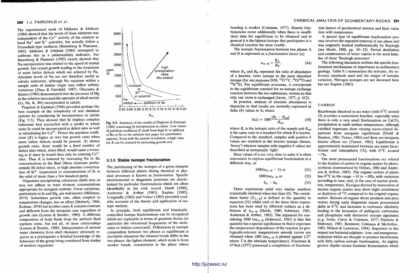
290 I.J. FAIRCHILD ef al.
T h e experimental work of Ishikawa & Ichikuni (1984) showed that the levels of these elements was independent of the C a 2 + activity of the solution at fixed N a + and K + activities, but actually follow a Freundlich-type isotherm (Busenberg & P lummer , 1985). Ishikawa & Ichikuni (1984) a t tempted to calibrate this as a palaeosalinity indicator , but Busenberg & Plummer (1985) clearly showed that Na incorporation was related to the speed of crystal growth, fast crystal growth leading to the formation of more lattice defects which are selected by Na . Absolute levels of Na are not therefore useful as salinity indicators, although Na variation within a sample suite of similar origin may reflect salinity variations (Zhao & Fairchild, 1987). O k u r a m a & Kitano (1986) demonstra ted that the presence of Mg in the solution increased the amounts of alkali metals (Li, Na , K, Rb) incorporated in calcite.
Pingitore & Eas tman (1986) provided perhaps the best example of the complexity of real chemical systems by considering Sr incorporat ion in calcite (Fig. 9.5). They showed that Sr displays complex behaviour best reconciled with a model in which some Sr could be incorporated in defect sites as well as substituting for C a 2 + . Hence the parti t ion coefficient (K) is higher at very fast growth rates when more lattice defects would be present . A t slower growth rates , there would be a fixed number of defect sites which, when filled, would cause a lowering in K since Sr would then only be entering C a 2 +
sites. Thus K is lowered by increasing Na or Ba concentrat ions in the fluid (these elements preferentially fill defect si tes), o r high absolute concentration of S r 2 + (equivalent to concentrat ions of Sr in the solid of more than a few hundred p p m ) .
Organisms precipitating calcareous shells may or may not adhere to trace element concentrat ions appropria te for inorganic systems. Grea t variat ions, particularly in Sr and Mg, are well known (Milliman, 1974). Sometimes growth ra te , often coupled to t empera ture changes, has an effect (Moberly, 1968; Kolesar , 1978) but in o the r cases K remains constant and different from the inorganic case regardless of growth rate (Lorens & Bender , 1980). A different composition of body fluids from the ambient fluid explains some, but not all, of these relationships (Lorens & Bender , 1980). Interpretat ion of ancient water chemistry from shell chemistry obviously requires as a prerequisi te a detailed knowledge of the behaviour of the group being considered from studies of modern organisms.
3500 \r
3000
0.04 0.06 0.08 0.10 0.12 0.14 0.16 0.18 0.20
Fig. 9.5. Summary of the results of Pingitore & Eastman (1986) concerning Sr incorporation in calcite. Low values of partition coefficient K result from high Sr or addition of Ba or Na to the solution (see paper for quantitative aspects). Even with Na present in solution, a high value for K can be restored by increasing growth rate.
9.3.6 Stable isotope fract ionation
The parti t ioning of the isotopes of a given element between different phases during chemical or physical processes is known as fractionation. Specific environmental or diagenetic processes are characterized by particular fractionations which are often identifiable in the rock record. Hoefs (1980), Anderson & Ar thu r (1983), Kaplan (1983), Longstaffe (1983) and Veizer (1983) provided readable accounts of the theory and application of isotope analysis.
In principle, both equilibrium and kinetically-controlled isotope fractionations can be recognized which are explicable in terms of quantum theory (in particular the vibrational frequencies of the molecules or lattices concerned) . Differences in isotopic composit ion between two phases a t equil ibrium is inevitable whenever the e lement bonds differ in the two phases: the lighter e lement , which tends to form weaker bonds , concentrates in the phase where
CHEMICAL ANALYSIS OF SEDIMENTARY ROCKS 291
bonding is weaker (Coleman, 1977). Kinetic fract ionations occur additionally when there is insufficient t ime for equilibrium to be obtained and in general it is t h e lightest isotope that participates in a chemical reaction the most readily.
T h e isotopic fractionation between two phases A and B is expressed as a fractionation factor ( a )
< * A - B — RA
RB' (4a)
where R A and R B represent the ratio of abundance of a heavier , rarer isotope to the most abundant isotope (for our purposes D / H , 1 3 C / 1 2 C , 1 8 0 / 1 6 0 and 3 4 S / 3 2 S ) . For equilibrium processes, a corresponds to the equilibrium constant for an isotope exchange reaction between the two substances, written so that only one a tom is exchanged (Javoy, 1977, p . 612).
In pract ice, analysis of absolute abundances is imprecise so that results are normally expressed as delta (5) values in %o where
b(x) = 1000 (RX - RST<J)
R. s t d (50)
where RX is the isotopic ratio of the sample and R s t a
is the same ratio in a s tandard for which R is known. Compared to the s tandard, samples with positive 5 values are enriched in the heavier isotope (hence, 'heavy') whereas samples with negative 6 values are described as isotopically 'light'.
Since values of a are very close to unity it is often convenient to express equilibrium fractionation in a different way, as
1 0 0 0 ( a A _ B - 1) or
1 0 0 0 1 n a A _ B or
6 A - 6 B
(51)
(52)
(53)
These expressions yield very similar numbers (essentially identical when less than 10). The enrichment factor ( £ A _ B ) is defined as the quantity in equat ion (51) whilst each of the these three expressions has been used by different authors as a definition of A A _ B (Hoefs, 1980; Schwarcz, 1981; Anderson & Ar thu r , 1983). T h e argument for considering 1000 l n a A _ B (Schwarcz, 1981) is that this quanti ty has a special significance in that it expresses the tempera ture-dependence of the reaction (at geologically-relevant tempera tures smooth curves are obtained when 1000 l n a A _ B is plot ted against 1/T2
where T is the absolute t empera ture ) . Fr iedman & O'Neil (1977) presented a compilation of fractiona
tion factors of geochemical interest and their variation with t empera ture .
A special type of equil ibrium fractionation process involves the repeated removal of one phase and was originally t reated mathematically by Rayleigh (see Hoefs , 1980, pp . 1 0 - 1 2 ) . Partial distillation and condensat ion of water vapour is the most familiar of these 'Rayleigh processes ' .
The following discussion outlines the specific fractionation mechanisms of impor tance in sedimentary geology. Table 9.1 summarizes the isotopes, the reference s tandards used and the ranges of isotopic variation. Nitrogen isotopes are not discussed here but see Kaplan (1983).
C A R B O N
Bicarbonate dissolved in sea water (with 5 I 3 C around O ) provides a convenient baseline, especially since there is only a very small fractionation on C a C 0 3
precipitation at earth surface temperatures, although calcified organisms show varying taxon-related depar tures from inorganic equilibrium (Dodd & Stanton, 1981; Veizer , 1983) and there are inorganic kinetic effects too (Turner , 1982). Equil ibrium is approximately maintained between sea water bicarbonate and atmospheric C 0 2 with 6 J 3 C around -7%».
The most pronounced fractionations are related to the fixation of carbon in organic mat ter by photosynthesis (summarized by Deines , 1980 and Ander son & Ar thur , 1983). The organic carbon of plants has 6 1 3 C in the range —10 to — 30%o with variations according to taxa, and, in the case of marine plankton, t empera tu re . Kerogen derived by maturat ion of mar ine organic mat ter may show slight enrichment or deplet ion of 1 3 C compared to the original organic mat ter . Release of organic decay products into pore waters during early diagenesis causes pronounced shifts in 5 1 3 C and increases in carbonate alkalinity leading to the formation of authigenic carbonates and phosphates with distinctive isotope signatures (e.g. Irwin, Curtis & Coleman, 1977; Pisciotto & Mahoney , 1981; B e n m o r e , Coleman & McAr thur , 1983; Nelson & Lawrence , 1984). Important in this respect are bacterial sulphate- , iron- and manganese-reduction which are thought to produce bicarbonate with little carbon isotope fractionation. A t slightly greater depths occurs bacterial fermentation which
http://jurassic.ru/
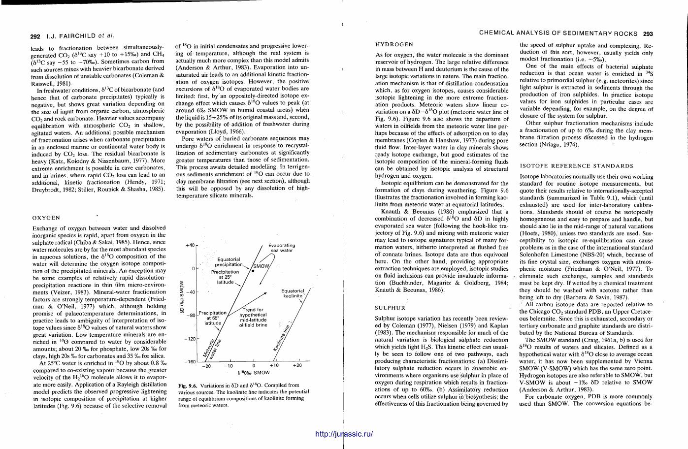
292 I.J. FAIRCHILD ET AL.
leads to fractionation between simultaneously-generated C O z ( 5 1 3 C say + 1 0 to + 15%,) and C H 4
( 6 1 3 C say - 5 5 to —70%o). Somet imes carbon from such sources mixes with heavier bicarbonate derived from dissolution of unstable carbonates (Coleman & Raiswell, 1981).
In freshwater condit ions, 5 1 3 C of bicarbonate (and hence that of carbonate precipitates) typically is negative, but shows great variation depending on the size of input from organic carbon, a tmospher ic C 0 2 and rock carbonate . Heavier values accompany equilibration with a tmospheric C 0 2 in shallow, agitated waters. A n additional possible mechanism of fractionation arises when carbonate precipitation in an enclosed marine or continental water body is induced by C 0 2 loss. The residual bicarbonate is heavy (Katz, Kolodny & Nissenbaum, 1977). M o r e ext reme enrichment is possible in cave carbonates , and in brines, where rapid C 0 2 loss can lead to an additional, kinetic fractionation (Hendy , 1971; Dreybrodt , 1982; Stiller, Rounick & Shasha, 1985).
O X Y G E N
Exchange of oxygen between water and dissolved inorganic species is rapid, apar t from oxygen in the sulphate radical (Chiba & Sakai, 1985). H e n c e , since water molecules are by far the most abundant species in aqueous solutions, the 5 l s O composition of the water will de termine the oxygen isotope composition of the precipitated minerals. An exception may be some examples of relatively rapid dissolution-precipitation reactions in thin film micro-environments (Veizer, 1983). Mineral-water fractionation factors are strongly tempera ture-dependent (Friedman & O'Neil , 1977) which, although holding promise of pa laeo tempera ture determinat ions , in practice leads to ambiguity of interpretat ion of isotope values since 8 i 8 0 values of natural waters show great variation. Low tempera ture minerals are enriched in , s O compared to water by considerable amounts ; about 20 %o for phospha te , low 20s %o for clays, high 20s %o for carbonates and 35 %o for silica.
At 25°C water is enriched in l 8 0 by about 0.8 % compared to co-existing vapour because the greater velocity of the H 2
1 6 0 molecule allows it to evaporate more easily. Application of a Rayleigh distillation model predicts the observed progressive lightening in isotopic composition of precipitation at higher latitudes (Fig. 9.6) because of the selective removal
of l s O in initial condensates and progressive lowering of t empera tu re , although the real system is actually much more complex than this model admits (Anderson & Ar thu r , 1983). Evaporat ion into unsaturated air leads to an additional kinetic fractionation of oxygen isotopes. However , the positive excursions of 5 I 8 0 of evaporated water bodies are limited: first, by an oppositely-directed isotope exchange effect which causes 6 l s O values to peak (at around 6%o S M O W in humid coastal areas) when the liquid is 15—25% of its original mass and, second, by the possibility of addition of freshwater during evaporat ion (Lloyd, 1966).
Pore waters of buried carbonate sequences may undergo 5 l s O enrichment in response to recrystallization of sedimentary carbonates at significantly greater tempera tures than those of sedimentat ion. This process awaits detailed modelling. In terrigenous sediments enr ichment of l s O can occur due to clay membrane filtration (see next section), although this will be opposed by any dissolution of high-tempera ture silicate minerals.
- 2 0 - 1 0 0 + 1 0 + 2 0
S180%o SMOW
Fig. 9.6. Variations in 8D and 8 l s O . Compiled from various sources. The kaolinite line indicates the potential range of equilibrium compositions of kaolinite forming from meteoric waters.
CHEMICAL ANALYSIS OF SEDIMENTARY ROCKS 293
H Y D R O G E N
As for oxygen, the water molecule is the dominant reservoir of hydrogen. T h e large relative difference in mass between H and deuter ium is the cause of the large isotopic variations in nature. The main fractionation mechanism is that of distillation-condensation which, as for oxygen isotopes, causes considerable isotopic lightening in the more extreme fractionation products . Meteoric waters show linear covariation on a 5 D — 8 1 8 0 plot (meteoric water line of Fig. 9.6). Figure 9.6 also shows the depar ture of waters in oilfields from the meteoric water line perhaps because of the effects of adsorption on to clay membranes (Coplen & Hanshaw, 1973) during pore fluid flow. Inter-layer water in clay minerals shows ready isotope exchange, but good estimates of the isotopic composit ion of the mineral-forming fluids can be obtained by isotopic analysis of structural hydrogen and oxygen.
Isotopic equilibrium can be demonst ra ted for the formation of clays during weathering. Figure 9.6 illustrates the fractionation involved in forming kaolinite from meteoric water at equatorial latitudes.
Knau th & Beeunas (1986) emphasized that a combinat ion of decreased 8 l s O and 8 D in highly evaporated sea water (following the hook-like trajectory of Fig. 9.6) and mixing with meteoric water may lead to isotope signatures typical of many formation waters , hi therto interpreted as flushed free of, connate brines. Isotope data are thus equivocal here . O n the other hand , providing appropr ia te extraction techniques are employed, isotopic studies oh fluid inclusions can provide invaluable information (Buchbinder , Magaritz & Goldberg , 1984; Knauth & Beeunas , 1986).
S U L P H U R
Sulphur isotope variation has recently been reviewed by Coleman (1977), Nielsen (1979) and Kaplan (1983). The mechanism responsible for much of the natural variation is biological sulphate reduction Which yields light H 2 S . This kinetic effect can usually be seen to follow one of two pathways, each producing characteristic fractionations: (a) Dissimi-latory sulphate reduction occurs in anaerobic environments where organisms use sulphur in place of oxygen during respiration which resul ts in fractionations of up to 60%o. (b) Assimilatory reduction occurs when cells utilize sulphur in biosynthesis: the effectiveness of this fractionation being governed by
the speed of sulphur uptake and complexing. Reduction of this sort, however , usually yields only modest fractionation (i .e. ~5%o).
O n e of the main effects of bacterial sulphate reduction is that ocean water is enriched in 3 4 S relative to primordial sulphur (e.g. meteori tes) since light sulphur is extracted in sediments through the product ion of iron sulphides. In practice isotope values for iron sulphides in particular cases are variable depending, for example , on the degree of closure of the system for sulphur.
O the r sulphur fractionation mechanisms include a fractionation of up to 6%o during the clay membrane filtration process discussed in the hydrogen section (Nriagu, 1974).
I S O T O P E R E F E R E N C E S T A N D A R D S
Isotope laboratories normally use their own working standard for routine isotope measurements , but quote their results relative to internationally-accepted s tandards (summarized in Table 9.1), which (until exhausted) are used for inter-laboratory calibrations. Standards should of course be isotopically homogeneous and easy to prepare and handle , but should also lie in the mid-range of natural variations (Hoefs, 1980), unless two standards are used. Susceptibility to isotopic re-equilibration can cause problems as in the case of the international standard Solenhofen Limestone (NBS-20) which, because of its fine crystal size, exchanges oxygen with atmospheric moisture (Fr iedman & O'Neil , 1977). To eliminate such exchange, samples and standards must be kept dry. If wet ted by a chemical t rea tment they should be washed with acetone rather than being left to dry (Barbera & Savin, 1987). : All carbon isotope data are reported relative to the Chicago C 0 2 s tandard P D B , an Uppe r Cretaceous belemnite. Since this is exhausted, secondary or tertiary carbonate and graphite standards are distributed by the National Bureau of Standards.
The S M O W standard (Craig, 1961a, b) is used for 8 l s O results of waters and silicates. Defined as a hypothetical water with 8 1 8 0 close to average ocean water , it has now been supplemented by Vienna S M O W (V-SMOW) which has the same zero point. Hydrogen isotopes are also referable to S M O W , but V - S M O W is about -1%„ 8 D relative to S M O W (Anderson & Ar thur , 1983).
For carbonate oxygen, P D B is more commonly used than S M O W . T h e conversion equat ions be-
http://jurassic.ru/
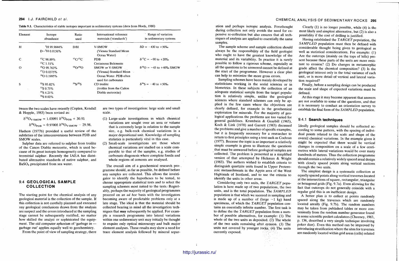
294 I . J . F A I R C H I L D ef al.
Table 9.1. Characteristics of stable isotopes important in sedimentary systems (data from Hoefs, 1980)
Element Isotope Ratio International reference Range of variation abundance used materials ('standards') in sedimentary systems
H 'H 99.9844% D = 2 H 0.0156%
D/H V-SMOW (Vienna Standard Mean Ocean Water)
8D = -430 to +50%o
C 1 2 C 98.89% 1 3 C 1 . 1 1 %
1 3 C/ 1 2 C PDB Cretaceous Belemnite
5 , 3 C = - 9 0 to +20%
O 1 6 0 99.763% 1 7 0 0.0375% l s O 0.1995%
1 8 0 / 1 6 0 SMOW or V-SMOW (Vienna) Standard Mean Ocean Water. PDB often used for carbonates
5 1 80 = - 4 5 to +40% SMOW
s 3 2 S 95.02% 3 3 S 0.75% 3 4 S 4.21% 3 6 S 0.02%
3 4 S / 3 2 S CD troilite (troilite from the Canon Diablo meteorite)
8 3 4 S = - 4 0 to +50%
tween the two scales have recently (Coplen, Kendall & H o p p l e , 1983) been revised as:
8 1 8 0 V - S M O W = 1-03091 8 1 8 O p d b + 30.91
8 1 8 O p d b = 0.97002 5 1 8 0 V - S M O W - 29.98.
Hudson (1977b) provided a useful review of the subtleties of the interconversions between P D B and S M O W scales.
Sulphur data are referred to sulphur from troilite of the Canon Diablo meteor i te , which is used because of its great isotopic homogenei ty compared to terrestrial sulphur. Recently the I A E A has distributed alternative s tandards of native sulphur, and B a S 0 4 precipitated from sea water .
9.4 G E O L O G I C A L S A M P L E C O L L E C T I O N
The starting point for the chemical analysis of any geological material is the collection of the sample . If this collection is not carefully planned and executed any geological conclusions drawn from the analysis are suspect and the errors introduced at the sampling stage cannot be subsequently rectified, no mat ter how skilled the analyst or sophisicated the equipment . The old computer aphorism of 'garbage in — garbage out ' applies equally well to geochemistry.
From the point of view of sampling strategy, there
are two types of investigation: large scale and small scale.
(1) Large-scale investigations in which chemical variations are sought over an area or volume that is extremely large in relation to the sample size, e.g. bulk-rock chemical variations in a major depositional unit. Knowledge of sampling statistics is particularly vital in this case.
(2) Small-scale investigations are those where chemical variations are studied on a scale comparable to that of the-samples , e.g. studies of carbonate diagenesis where complete fossils and whole regions of cements are analysed.
T h e overall aim of a geochemical research programme should, as far as possible, be defined before any samples are collected. This allows the investigator to identify the hypotheses to be tested, to choose appropr ia te statistical tests and to select the sampling schemes most suited to the tests / .Regret-ably, perhaps the majority of geological p rogrammes proceed on an ad hoc basis with the investigators becoming aware of predictable problems only at a late stage. The ideal is that the material should be collected bearing in mind all the investigation techniques that may subsequently be applied. For example a research p rogramme into lateral variations within one sedimentary unit may initially be thought to require only optical microscopy and bulk major e lement analyses. These results may show a need for t race element analysis followed by mineral separ-
1 C H E M I C A L A N A L Y S I S O F S E D I M E N T A R Y R O C K S 295
ation and perhaps isotopic analysis. Forethought during collection not only avoids the need for expensive re-collection but also ensures that all techniques of analysis are applied to essentially the same samples.
T h e sample scheme and sample collection should always be the responsibility of the field geologist w h o ought t o have the greatest knowledge of the material and its variability. In practice it is rarely possible to follow a r igorous scheme, especially as all the questions to be answered cannot be defined at the start of the p rogramme. However a clear p lan can help to minimize the more gross errors .
Sampling schemes have been mainly developed by statisticians working in the social sciences or in biometrics. In these subjects the collection of an adequate statistical sample from the target population is relatively simple, unlike the geological sciences where s tandard schemes can only be applied in the few cases where the objectives are clearly defined, for example in the geochemical exploration for minerals . For the majority of geological applications the problems are too varied for general guidelines. Krumbein & Graybill (1965), Koch & Link (1970) and Gar re t t (1983) discussed the problems and give a number of specific examples , bu t it is frequently necessary for a researcher t o re turn to first principles using a text such as Cochran (1977). Because the topic is so important a relatively simple example is given to illustrate the questions that must be answered before geological samples are collected. The problem is presented as a simplified version of that a t tempted by Hickman & Wright (1983). The authors wished to establish criteria to distinguish quartzite units found in Uppe r Protero-zoic rrtetasediments in the Appin area of the West Highlands of Scotland, and to use the criteria to identify the units in o ther areas.
Considering only two units, the TARGET population is here made up of two populat ions, the two units, and is the total populat ion. The SAMPLED populat ion is that which we succeed in sampling and is made up of a number of (large ~ 1 kg) hand specimens, of which the TARGET populat ion contains an essentially infinite number . The first task is to define the the TARGET populat ion from a number of possible alternatives, for example: (1) The whole of the two units as deposi ted. (2) T h e whole of the two units remaining after erosion. (3) The units not covered by younger rocks. (4) The units currently exposed. ' .
Clearly (1) is n o longer possible, while (4) is t he most likely and simplest al ternative, but (2) is also a possibility if the cost of drilling is justified.
Having established the TARGET populat ion, the SAMPLED populat ion must then be defined with considerable thought being given to geological as well as statistical considerations. For example: (1) A r e the outcrops (mainly on the tops of hills) present because these parts of the units are more resistant to erosion? (2) D o changes in metamorphic grade affect the chemical composit ion? (3) Is the geological interest only in the total variance of each unit , or is more detail of vertical and lateral variat ion required?
Finally, before a sampling design can be produced the scale and shape of expected variations must b e defined.
A t this stage it may become apparent that answers are not available to some of the questions, and that it is necessary to conduct an orientat ion survey to establish the final form of the SAMPLED population.
9.4.1 Search techniques
Ideally geological samples should be collected according to some pat tern , with the spacing of individual points related t o t he scale and shape of the overall chemical variations. In the example given it might be expected tha t there would be vertical changes in composit ion on a scale of a few centimetres while lateral variations would be over many hundreds of metres . Thus the collection programme should contain a relatively widely spaced areal design with closely spaced points along vertical sections through the two units.
The simplest design is a systematic collection at equally spaced points along vertical traverses located at t he intersections of square , rectangular, triangular or hexagonal grids (Fig. 9.7a). Even allowing for the fact tha t outcrops d o no t generally coincide with a regular grid this is an inefficient design.
A bet ter plan is to collect a t points randomly spaced along the traverses which are randomly located areally (Fig. 9.7b). The random numbers may be taken from published tables or more conveniently from the random number generator found in some scientific pocket calculators (Cheeney, 1983, p . 136, described a very simple technique involving poker dice). Even this method can be improved by introducing stratification where the sites for traverses are randomly located within grid areas (cells) related
http://jurassic.ru/
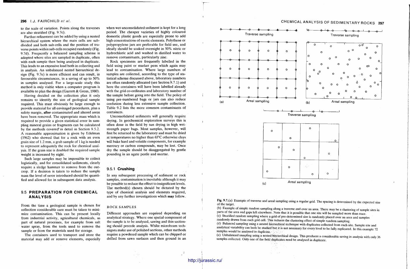
296 I.J. FAIRCHILD et al.
to the scale of variation. Points along the traverses are also stratified (Fig. 9.7c).
Fur ther refinement can be added by using a nested hierarchical system where the main cells are subdivided and both sub-cells and the position of traverse points within sub-cells occupied randomly (Fig. 9.7d). Frequently a balanced sampling scheme is adopted where sites are sampled in duplicate, often with each sample then being analysed in duplicate. This leads to an excessive load both in collecting and in analysis. A n unbalanced nested hierarchical design (Fig. 9.7e) is more efficient and can result, in favourable circumstances, in a saving of up to 5 0 % in samples analysed. For a large-scale study this method is only viable when a computer program is available to plan the design (Garre t t & Gross , 1980).
Having decided on the collection plan it only remains to identify t he size of geological sample required. This must obviously be large enough to provide material for all envisaged procedures , plus a safety margin, after contaminated and altered areas have been removed. The appropria te mass which is required to provide a given statistical error in sampling mineral grains or fragments can be calculated by the methods covered* in detail in Section 9.5.2. A reasonable approximation is given by Ede lman (1962) who showed that for a rock with an even grain size of 1.2 m m , a grab sample of 1 kg is needed to represent adequately the rock for chemical analysis. If the grain size is doubled the required sample weight is increased by eight.
Such large samples may be impossible to collect logistically, and for consolidated sediments , clearly require a sledge hammer to remove from the outcrop. If a decision is taken to reduce the sample mass the level of error introduced should be quantified and allowed for in subsequent data analysis.
9.5 P R E P A R A T I O N FOR C H E M I C A L A N A L Y S I S
From the time a geological sample is chosen for collection considerable care must be taken to minimize contaminat ion. This can be present locally from industrial activity, agricultural chemicals, as part of natural processes, for example from salt water spray, from the tools used to remove the sample or from the materials used for storage.
The containers used to transport and store the material may add or remove elements , especially
when wet unconsolidated sediment is kept for a long period. T h e cheaper varieties of highly coloured domestic plastic goods are especially p rone to add high concentrat ions of exotic e lements . Polythene or polypropylene jars are preferable for field use, and ideally should be soaked overnight in 5 0 % nitric or hydrochloric acid and washed in distilled water to remove contaminants , particularly zinc.
Rock specimens are frequently labelled in the field using paint or marker pens which again may lead to contaminat ion. Where large numbers of samples are collected, according to the type of statistical scheme discussed above, laboratory numbers are often randomly allocated (see Section 9.7.1) and here the containers will have been labelled already with the grid co-ordinates and laboratory number of the sample before going into the field. T h e policy of using pre-numbered bags or jars can also reduce confusion during less extensive sample collection. Table 9.2 lists the more common contaminants of containers.
Unconsol idated sediments will generally require drying. In geochemical exploration surveys this is often done in the field by sun drying in high wet-strength paper bags. Most samples , however , will first be re turned to the laboratory and must be dried at tempera tures no higher than 65°C otherwise clays will bake hard and volatile components , for example mercury or carbon compounds , may be lost. Once dry the sample should be disaggregated by gentle pounding in an agate pestle and mor ta r .
9.5.1 Crushing
In any subsequent processing of sediment or rock samples, contaminat ion is inevitable al though it may be possible to reduce the effect to insignificant levels. T h e method(s) chosen should be dictated by the type of chemical analysis and elements required, and by any further investigations which may follow.
R O C K S A M P L E S
Different approaches are required depending on analytical strategy. Where one spatial component of the sample is to be analysed, sawing and thin sectioning should precede analysis. Whilst microbeam techniques make use of polished sections, o ther methods require a powdered sample which can be chipped or drilled from sawn surfaces and then ground in an
CHEMICAL ANALYSIS OF SEDIMENTARY ROCKS 297
- 9 -
Traverse sampling >©- 6 1 o—©- - t9 e—e— 1—e ©-
Traverse sampling
o e 1
o o
<) ©- 1
> e 1
) o <
i .
> © 1
1 0
> © a
> O ( 1
O 0 (
O 0 c
' U 1
> 0 <
1 © <
> 0 (
> © o
> o o
<) 0 <
© © <
' t r (
1 o <
> © <
> © 1
> O (
> e <
> © o
> O ( )
) © © (a) Areal sampling
o o
o o o 0
CO o o
O O
o o u o o
6 o ° ° o o
0 ° o ° o
L 2 . o o (b) Areal sampling
—©—i— Traverse sampling
(0 Areal sampling
Fig. 9.7.(a) Example of traverse and areal sampling using a regular grid. The spacing is determined by the expected size of the target. (b) Example of simple random sampling along a traverse and over an area. There may be a clustering of sample sites in parts of the area and gaps left elsewhere. Note that it is possible that one site will be sampled more than once. (c) Stratified random sampling where a grid of pre-determined size is randomly placed over an area and samples randomly drawn from each grid cell. This reduces the clustering effect of simple random sampling. (d) Balanced sampling using a nested hierarchical technique with duplicates collected from each site. Sample site and analytical variability can both be studied but it is not necessary for every level to be fully replicated. In this example 72 samples would be analysed in duplicate. : • -(e) Unbalanced sampling using a nested hierarchical design. This produces a considerable saving in analysis with only 36 samples collected. Only one of the field duplicates need be analysed in duplicate.
u
http://jurassic.ru/
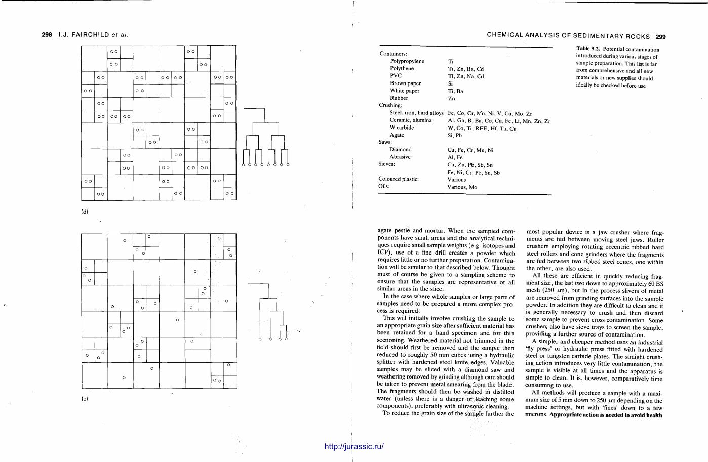
298 I.J. F A I R C H I L D ef AL.
O 0 o o
o o 0 o
0 0 o o 0 o o o o o 0 o
0 O o o
o o o o
0 o oo 0 o o o
o o O 0
o o o o
o o O 0
o o o o o o o o
O o o o o o
o o o o o o
6
(d)
o 0 o o
o o
o o
o o o
o
o
o
o 0
o o
0
o o
o o
o o o
o
o
o o
o
o o o o
o o o
o o
o o
(e)
C H E M I C A L A N A L Y S I S OF S E D I M E N T A R Y R O C K S 299
Containers: Polypropylene Ti Polythene Ti, Zn, Ba, Cd PVC Ti, Zn, Na, Cd Brown paper Si White paper Ti, Ba Rubber Zn
Crushing: Steel, iron, hard alloys Fe, Co, Cr, Mn, Ni, V, Cu, Mo, Zr Ceramic, alumina W carbide Agate
Saws: Diamond Abrasive
Sieves:
Coloured plastic: Oils:
Al, Ga, B, Ba, Co, Cu, Fe, Li, Mn, Zn, Zr W, Co, T i ,REE, Hf,Ta, Cu Si, Pb
Cu, Fe, Cr, Mn, Ni Al, Fe Cu, Zn, Pb, Sb, Sn Fe, Ni, Cr, Pb, Sn, Sb Various Various, Mo
Table 9.2. Potential contamination introduced during various stages of sample preparation. This list is far from comprehensive and all new materials or new supplies should ideally be checked before use
agate pestle and mortar . When the sampled components have small areas and the analytical techniques require small sample weights (e.g. isotopes and ICP) , use of a fine drill creates a powder which requires little or n o further preparat ion. Contamination will be similar to that described below. Thought must of course be given to a sampling scheme to ensure that the samples are representat ive of all similar areas in the slice.
In the case where whole samples or large parts of samples need to be p repared a more complex process is required.
This will initially involve crushing the sample to an appropria te grain size after sufficient material has been retained for a hand specimen and for thin sectioning. Wea the red material not t r immed in the field should first be removed and the sample then reduced to roughly 50 m m cubes using a hydraulic splitter with ha rdened steel knife edges . Valuable samples may be sliced with a d iamond saw and weathering removed by grinding although care should be taken to prevent meta l smearing from the b lade . T h e fragments should then be washed in distilled water (unless there is a danger of leaching some components ) , preferably with ultrasonic cleaning.
T o reduce the grain size of the sample further the
most popular device is a jaw crusher where fragments are fed between moving steel jaws. Roller crushers employing rotating eccentric ribbed hard steel rollers and cone grinders where the fragments are fed between two ribbed steel cones, one within t he o ther , a re also used.
All these are efficient in quickly reducing fragm e n t size, the last two down to approximately 60 BS mesh (250 um) , but in the process slivers of metal are removed from grinding surfaces into the sample powder . In addition they are difficult to clean and it is generally necessary to crush and then discard some sample to prevent cross contaminat ion. Some crushers also have sieve trays to screen the sample, providing a further source of contaminat ion.
A simpler and cheaper method uses an industrial 'fly press ' or hydraulic press fitted with hardened steel or tungsten carbide plates. The straight crushing action introduces very little contaminat ion, the sample is visible at all t imes and the apparatus is simple t o clean. I t is, however , comparatively t ime consuming to use.
All me thods will p roduce a sample with a maximum size of 5 mm down to 250 um depending on the machine sett ings, but with 'fines' down to a few microns. Appropriate action is needed to avoid health
http://jurassic.ru/
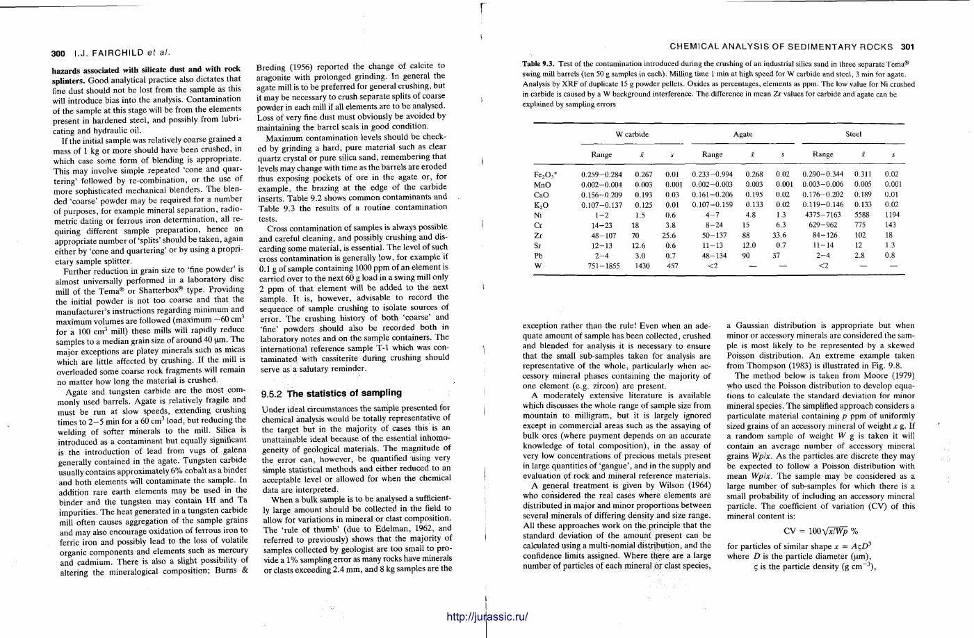
300 I.J. FAIRCHILD ef al.
hazards associated with silicate dust and with rock splinters. G o o d analytical practice also dictates that fine dust should not be lost from the sample as this will introduce bias into the analysis. Contaminat ion of the sample at this stage will be from the e lements present in hardened steel, and possibly from lubricating and hydraulic oil.
If the initial sample was relatively coarse grained a mass of 1 kg or more should have been crushed, in which case some form of blending is appropr ia te . This may involve simple repeated 'cone and quartering' followed by re-combinat ion, o r the use of more sophisticated mechanical blenders . T h e blended 'coarse ' powder may be required for a number of purposes , for example mineral separat ion, radiometric dat ing or ferrous iron de terminat ion , all requiring different sample prepara t ion , hence an appropria te number of 'splits' should be t aken , again either by 'cone and quar ter ing ' or by using a proprietary sample splitter.
Fur ther reduction in grain size to 'fine powder ' is almost universally performed in a laboratory disc mill of the Tema® or Shatterbox® type. Providing the initial powder is not too coarse and that the manufacturer 's instructions regarding minimum and maximum volumes are followed (maximum ~ 6 0 c m 3
for a 100 c m 3 mill) these mills will rapidly reduce samples to a median grain size of a round 40 um. T h e major exceptions are platey minerals such as micas which are little affected by crushing. If the mill is overloaded some coarse rock fragments will remain no mat ter how long the material is crushed.
Agate and tungsten carbide are the most commonly used barrels . Agate is relatively fragile and must be run at slow speeds, extending crushing times to 2—5 min for a 60 c m 3 load, but reducing the welding of softer minerals to the mill. Silica is introduced as a contaminant but equally significant is the introduction of lead from vugs of galena generally contained in the agate . Tungsten carbide usually contains approximately 6% cobalt as a binder and both elements will contaminate the sample . In addition rare ear th elements may be used in the binder and the tungsten may contain Hf and T a impurities. The heat generated in a tungsten carbide mill often causes aggregation of the sample grains and may also encourage oxidation of ferrous iron t o ferric iron and possibly lead to the loss of volatile organic components and elements such as mercury and cadmium. The re is also a slight possibility of altering the mineralogical composit ion; Burns &
Breding (1956) repor ted the change of calcite to aragonite with prolonged grinding. In general the agate mill is to be preferred for general crushing, but it may be necessary to crush separate splits of coarse powder in each mill if all elements are to be analysed. Loss of very fine dust must obviously be avoided by maintaining the barrel seals in good condition.
Maximum contaminat ion levels should be checked by grinding a hard , pu re material such as clear quar tz crystal or pure silica sand, remember ing that levels may change with t ime as the barrels are e roded thus exposing pockets of ore in the agate or , for example , the brazing at the edge of the carbide inserts. Tab le 9.2 shows common contaminants and Table 9.3 the results of a routine contaminat ion tests .
Cross contaminat ion of samples is always possible and careful cleaning, and possibly crushing and discarding some mater ia l , is essential. The level of such cross contaminat ion is generally low, for example if 0.1 g of sample containing 1000 ppm of an e lement is carried over to the next 60 g load in a swing mill only 2 p p m of that e lement will b e added to the next sample. It is, however , advisable to record the sequence of sample crushing to isolate sources of er ror . T h e crushing history of bo th 'coarse ' and 'fine' powders should also be recorded both in laboratory notes and on the sample containers . T h e international reference sample T - l which was contaminated with cassiterite during crushing should serve as a salutary reminder .
9.5.2 The stat ist ics of sampl ing
U n d e r ideal circumstances the sample presented for chemical analysis would be totally representat ive of the target but in the majority of cases this is an unat ta inable ideal because of t he essential inhomo-geneity of geological materials. The magni tude of the error can, however , be quantified using very simple statistical me thods and ei ther reduced to an acceptable level or allowed for when the chemical da ta are interpreted.
When a bulk sample is to be analysed a sufficiently large amount should be collected in the field to allow for variations in mineral or clast composi t ion. T h e 'rule of t humb ' (due to Ede lman , 1962, and referred to previously) shows that the majori ty of samples collected by geologist are too small to provide a 1% sampling error as many rocks have minerals or clasts exceeding 2.4 m m , and 8 kg samples are the
CHEMICAL ANALYSIS OF SEDIMENTARY ROCKS 301
Table 9.3. Test of the contamination introduced during the crushing of an industrial silica sand in three separate Tema® swing mill barrels (ten 50 g samples in each). Milling time 1 min at high speed for W carbide and steel, 3 min for agate. Analysis by XRF of duplicate 15 g powder pellets. Oxides as percentages, elements as ppm. The low value for Ni crushed in carbide is caused by a W background interference. The difference in mean Zr values for carbide and agate can be explained by sampling errors
W carbide Agate Steel
Range X s Range X s Range X 5
F e 2 0 3 * 0.259-0.284 0.267 0.01 0.233-0.994 0.268 0.02 0.290-0.344 0.311 0.02 MnO 0.002-0.004 0.003 0.001 0.002- 0.003 0.003 0.001 0.003-0.006 0.005 0.001 CaO 0.156-0.209 0.193 0.03 0.161-0.206 0.195 0.02 0.176-0.202 0.189 0.01 K 2 0 0.107-0.137 0.125 0.01 0.107-0.159 0.133 0.02 0.119-0.146 0.133 0.02 Ni 1-2 1.5 0.6 4 - 7 4.8 1.3 4375-7163 5588 1194 Cr 14-23 18 3.8 8-24 15 6.3 629-962 775 143 Zr 48-107 70 25.6 50-137 88 33.6 84-126 102 18 Sr 12-13 12.6 0.6 11-13 12.0 0.7 11-14 12 1.3 Pb 2 - 4 3.0 0.7 48-134 90 37 2 - 4 2.8 0.8 W 751-1855 1430 457 <2 — — <2 — —
exception rather than the rule! Even when an adequate amount of sample has been collected, crushed and blended for analysis it is necessary to ensure that the small sub-samples taken for analysis are representat ive of the whole , particularly when accessory mineral phases containing the majority of one element (e.g. zircon) are present .
A moderately extensive l i terature is available which discusses the whole range of sample size from mountain to milligram, but it is largely ignored except in commercial areas such as the assaying of bulk ores (where payment depends on an accurate knowledge of total composi t ion) , in the assay of very low concentrat ions of precious metals present in large quantit ies of 'gangue ' , and in the supply and evaluation of rock and mineral reference materials.
A general t rea tment is given by Wilson (1964) who considered the real cases where elements are distributed in major and minor proport ions between several minerals of differing density and size range. All these approaches work on the principle that the standard deviation of the amount present can be calculated using a multi-nomial distribution, and the confidence limits assigned. Where there are a large number of particles of each mineral or clast species,
a Gaussian distribution is appropria te but when minor or accessory minerals are considered the sample is most likely to be represented by a skewed Poisson distribution. A n extreme example taken from Thompson (1983) is illustrated in Fig. 9.8.
The method below is taken from Moore (1979) who used the Poisson distribution to develop equations to calculate the s tandard deviation for minor mineral species. The simplified approach considers a particulate material containing p ppm of uniformly sized grains of an accessory mineral of weight x g. If a r andom sample of weight W g is taken it will contain an average number of accessory mineral grains Wp/x. As the particles are discrete they may be expected to follow a Poisson distribution with mean Wp/x. The sample may be considered as a large number of sub-samples for which there is a small probability of including an accessory mineral particle. T h e coefficient of variation (CV) of this mineral content is:
CV = lOOV^Wp %
for particles of similar shape x = AqD3
where D is the particle diameter (um) , c, is the particle density (g c m - 3 ) ,
http://jurassic.ru/
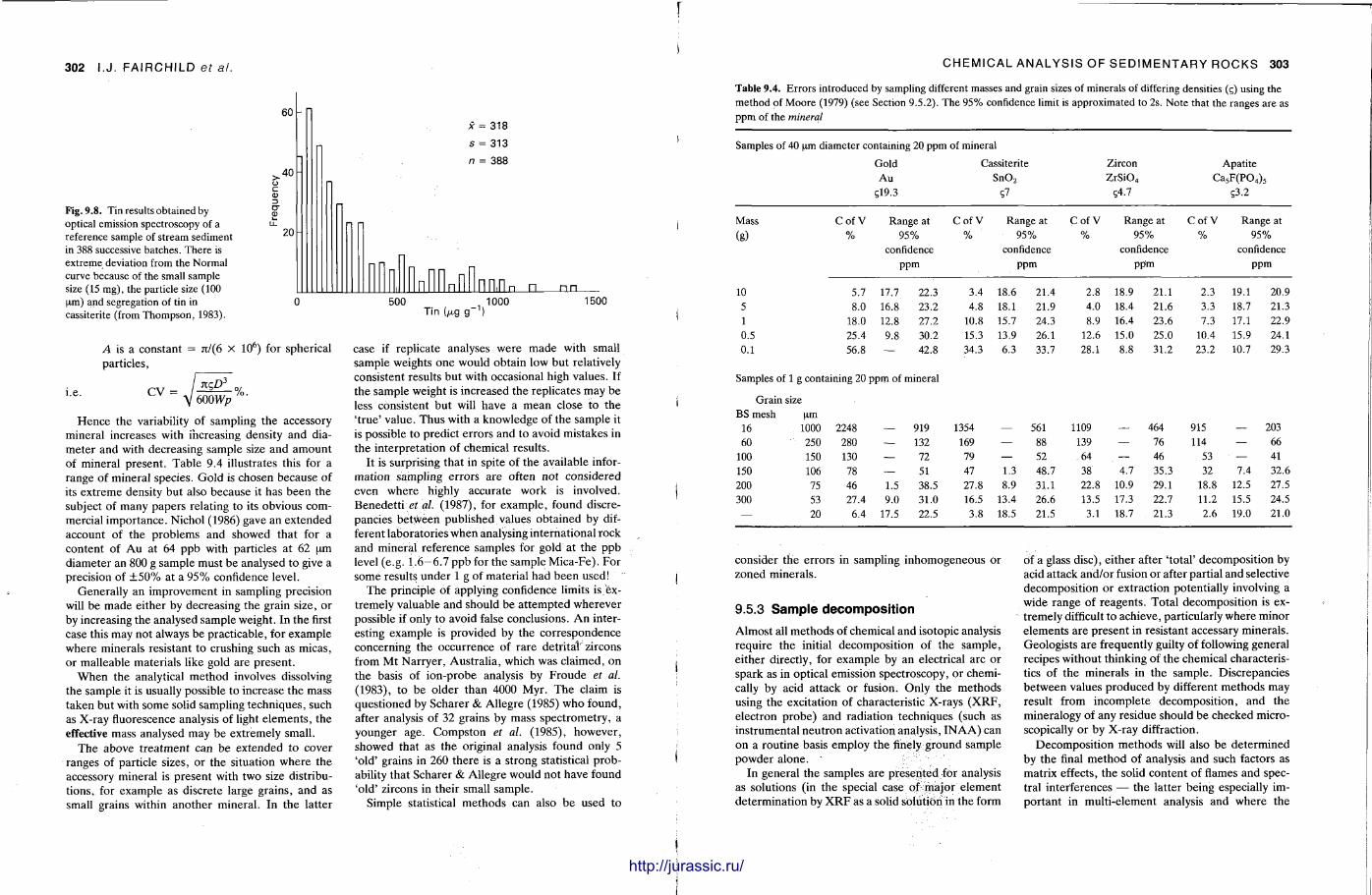
302 I.J. FAIRCHILD et al.
Fig. 9.8. Tin results obtained by optical emission spectroscopy of a reference sample of stream sediment in 388 successive batches. There is extreme deviation from the Normal curve because of the small sample size (15 mg), the particle size (100 um) and segregation of tin in cassiterite (from Thompson, 1983).
60
40
0)
cr CD
20
x = 318
s = 313
n = 388
LU nnrin n o n 500 1000
Tin (fig g n) 1500
A is a constant = ir/(6 x 10 6) for spherical particles,
Hence the variability of sampling the accessory mineral increases with increasing density and diameter and with decreasing sample size and amount of mineral present . Table 9.4 illustrates this for a range of mineral species. Gold is chosen because of its extreme density but also because it has been the subject of many papers relating to its obvious commercial importance . Nichol (1986) gave an extended account of the problems and showed that for a content of Au at 64 ppb with particles at 62 um diameter an 800 g sample must be analysed to give a precision of ± 5 0 % at a 9 5 % confidence level.
Generally an improvement in sampling precision will be made either by decreasing the grain size, or by increasing the analysed sample weight. In the first case this may not always be practicable, for example where minerals resistant to crushing such as micas, or malleable materials like gold are present .
When the analytical method involves dissolving the sample it is usually possible to increase the mass taken but with some solid sampling techniques, such as X-ray fluorescence analysis of light e lements , the effective mass analysed may be extremely small.
The above t reatment can be extended to cover ranges of particle sizes, or the situation where the accessory mineral is present with two size distributions, for example as discrete large grains, and as small grains within another mineral . In the latter
case if replicate analyses were made with small sample weights one would obtain low but relatively consistent results but with occasional high values. If the sample weight is increased the replicates may be less consistent but will have a mean close to the ' t rue ' value. Thus with a knowledge of the sample it is possible to predict errors and to avoid mistakes in the interpretat ion of chemical results.
It is surprising that in spite of the available information sampling errors are often not considered even where highly accurate work is involved. Benedet t i et al. (1987), for example , found discrepancies between published values obtained by different laboratories when analysing international rock and mineral reference samples for gold at the ppb level (e.g. 1.6—6.7 ppb for the sample Mica-Fe) . For some results under 1 g of material had been used!
The principle of applying confidence limits is extremely valuable and should be a t tempted wherever possible if only to avoid false conclusions. A n interesting example is provided by the correspondence concerning the occurrence of rare det r i ta l zircons from Mt Narryer , Austral ia, which was claimed, on the basis of ion-probe analysis by Froude et al. (1983), to be older than 4000 Myr. The claim is quest ioned by Scharer & Allegre (1985) who found, after analysis of 32 grains by mass spectrometry, a younger age. Compston et al. (1985), however , showed that as the original analysis found only 5 'old ' grains in 260 there is a strong statistical p robability that Scharer & Allegre would not have found 'old' zircons in their small sample.
Simple statistical methods can also be used to
CHEMICAL ANALYSIS OF SEDIMENTARY ROCKS 303
Table 9.4. Errors introduced by sampling different masses and grain sizes of minerals of differing densities (g) using the method of Moore (1979) (see Section 9.5.2). The 95% confidence limit is approximated to 2s. Note that the ranges are as ppm of the mineral
Samples of 40 urn diameter containing 20 ppm of mineral
Gold Cassiterite Zircon Apatite Au S n 0 2 ZrSi0 4 Ca 5 F(P0 4 ) 5
gl9.3 ?7 S4.7 5 3.2
Mass Cof V Range at Cof V Range at Cof V Range at C o f V Ran; *e at (g) % 95% % 95% % 95% % 95%
confidence confidence confidence confidence ppm ppm PPm ppm
10 5.7 17.7 22.3 3.4 18.6 21.4 2.8 18.9 21.1 2.3 19.1 20.9 5 8.0 16.8 23.2 4.8 18.1 21.9 4.0 18.4 21.6 3.3 18.7 21.3 1 18.0 12.8 27.2 10.8 15.7 24.3 8.9 16.4 23.6 7.3 17.1 22.9 0.5 25.4 9.8 30.2 15.3 13.9 26.1 12.6 15.0 25.0 10.4 15.9 24.1 0.1 56.8 — 42.8 34.3 6.3 33.7 28.1 8.8 31.2 23.2 10.7 29.3
Samples of 1 g containing 20 ppm of mineral
Grain size BS mesh um
16 1000 2248 — 919 1354 — 561 1109 — 464 915 — 203 60 250 280 — 132 169 — 88 139 — 76 114 — 66
100 150 130 — 72 79 — 52 64 — 46 53 — 41 150 106 78 — 51 47 1.3 48.7 38 4.7 35.3 32 7.4 32.6 200 75 46 1.5 38.5 27.8 8.9 •31.1 22.8 10.9 29.1 18.8 12.5 27.5 300 53 27.4 9.0 31.0 16.5 13.4 26.6 13.5 17.3 22.7 11.2 15.5 24.5 — 20 6.4 17.5 22.5 3.8 18.5 21.5 3.1 18.7 21.3 2.6 19.0 21.0
consider the errors in sampling inhomogeneous or zoned minerals.
9.5.3 Sample decomposi t ion
Almost all methods of chemical and isotopic analysis require the initial decomposit ion of the sample, either directly, for example by an electrical arc or spark as in optical emission spectroscopy, or chemically by acid attack or fusion. Only the methods using the excitation of characteristic X-rays ( X R F , electron probe) and radiation techniques (such as instrumental neutron activation analysis, I N A A ) can on a routine basis employ the finely ground sample powder alone.
In general the samples are presented for analysis as solutions (in the special case of major e lement determinat ion by X R F as a solid solution in the form
of a glass disc), ei ther after ' total ' decomposit ion by acid attack and/or fusion or after partial and selective decomposit ion or extraction potentially involving a wide range of reagents . Total decomposit ion is extremely difficult to achieve, particularly where minor e lements are present in resistant accessary minerals. Geologists are frequently guilty of following general recipes without thinking of the chemical characteristics of the minerals in the sample. Discrepancies be tween values produced by different methods may result from incomplete decomposi t ion, and the mineralogy of any residue should be checked microscopically or by X-ray diffraction.
Decomposi t ion methods will also be determined by the final method of analysis and such factors as matrix effects, the solid content of flames and spectral interferences — the latter being especially important in multi-element analysis and where the
http://jurassic.ru/
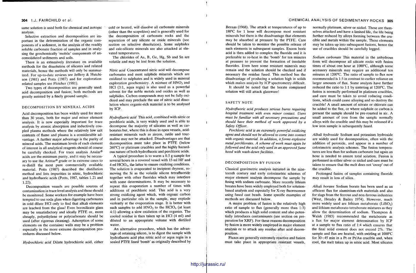
304 I.J. FAIRCHILD et al.
same solution is used both for chemical and isotopic analysis.
Selective extraction and decomposit ion a re impor tant in the determinat ion of the organic components of a sediment , in the analysis of the readily soluble carbonate fraction of samples and in analysing the geochemically 'mobile ' components of unconsolidated sediments and soils.
There is an extensively l i terature on available methods for the dissolution of silicates and related materials , hence the methods will only be summarized. For up-to-date reviews see Jeffery & Hutchison (1981) and Potts (1987) and for exploration-related samples see Fletcher (1981).
Two types of decomposit ion are generally used: acid decomposit ion and fusion; both methods a re greatly assisted by a finely ground sample .
D E C O M P O S I T I O N BY M I N E R A L A C I D S
Acid decomposit ion has been widely used for more than 30 years , both for major and minor e lement analysis. It is now especially impor tant for t race analysis by atomic absorption and inductively coupled plasma methods where the relatively low salt contents of flame and plasma is a considerable advantage. A further major advantage is the purity of mineral acids. T h e maximum levels of each element of interest in all analytical reagents should of course be carefully checked. For trace analysis Analar® acids are the minimum purity, and it may be necessary to use the Aristar® grade or in ext reme cases to re-distill the most pure commercially available material . Potts (1987) described the distillation method and lists impurit ies in nitric, hydrochloric and hydrofluoric acids (Pot ts , 1987, tables 1.21 and 1.22).
Decomposi t ion vessels are possible sources of contaminat ion in trace level analysis and these should be moni tored. Some workers for example have been tempted to use soda glass when digesting carbonates in cold dilute HC1 only to find that alkali e lements are leached from the glass! Even borosilicate glass may be unsatisfactory and ideally P T F E or , more cheaply, polyethylene or polycarbonate should be used (after rigorous cleaning). Adsorpt ion of some elements on the container walls may be a problem especially in the more ext reme decomposit ion procedures discussed below.
Hydrochloric acid Dilute hydrochloric acid, either
cold or hea ted , will dissolve all carbonate minerals (other than the scapolites) and is generally used for the decomposit ion of carbonate rocks and the separation of any silicate or oxide minerals (see section on selective dissolution). Some sulphides and calc-silicate minerals are also at tacked at elevated tempera tures .
The chlorides of As , B , G e , H g , Sb and Sn are volatile and may be lost from the solution.
Nitric acid Concentra ted nitric acid will decompose carbonates and most sulphide minerals which are oxidized to sulphates and is widely used in mineral exploration geochemistry. A mixture of H N 0 3 and HC1 (3 :1 , aqua regia) is also used as a powerful solvent for the noble metals and oxides as well as sulphides. Carbon compounds may not be fully oxidized and may preclude the use of nitric acid dissolution where organic-rich material is to b e analysed by ICP .
Hydrofluoric acid This acid, combined with nitric or perchloric acids, is very widely used and is able to decompose the majority of silicates as well as carbonates but , where this is done in open vessels, acid-resistant minerals such as zircon, rutile and tourmaline may not be at tacked. Disadvantages are that decomposit ion must take place in P T F E (below 260°C) or platinum crucibles and the highly hazardous nature of both hydrofluoric and perchloric acids.
A typical procedure is to warm a 0.5 g sample for several hours in a covered vessel with 15 ml H F and 4 ml H C 1 0 4 , the latter to ensure oxidizing conditions. The solution is evaporated to incipient dryness, removing the Si as the volatile silicon tetrafluoride together with o the r fluorides which may interfere with some determinat ions. It may be necessary to repeat this evaporat ion a number of t imes with additions of perchloric acid. This acid is a very strong oxidizing agent which, with organic carbon and in particular oils in the sample, may explode violently at the evaporat ion stage. It is bet ter with such samples to add H N 0 3 to the HCIO4 (at least 4:1) allowing a slow oxidation of the organics. The cooled residue is then taken up in HC1 (4 ml) and diluted t o an appropr ia te volume with distilled water .
A n alternative procedure , which has the advantage of retaining silicon, is to digest the sample with hydrofluoric acid plus nitric acid or aqua regia in a sealed P T F E lined ' b o m b ' as originally described by
CHEMICAL ANALYSIS OF SEDIMENTARY ROCKS 305
Bernas (1968). The attack at temperatures of up to 180°C for 1 hour will decompose most resistant minerals but there is the disadvantage that elements may be absorbed at pressure by the P T F E . Care should be taken to moni tor the possible release of such elements in subsequent samples. Excess boric acid is then added to complex the fluoride and it is preferable to re-heat in the ' b o m b ' for ten minutes at pressure to prevent the formation of insoluble fluorides. Even here some resistant minerals may remain and the solution should be checked and if necessary the residue fused. This method has the disadvantage of producing a solution high in solids which makes analysis by ICP spectrometry difficult.
I t should be noted that the bora te complexed solution will still at tack glassware!
S A F E T Y N O T E
Hydrofluoric acid produces serious burns requiring hospital treatment with even minor contact. Users must be familiar with all necessary precautions and should have their method of work approved by a Safety Officer.
Perchloric acid is an extremely powerful oxidizing agent and should not be allowed to come into contact with organic material. In addition, it forms explosive metal perchlorates. A scheme of work must again be followed and the acid only used in an approved fume hood with wash-down facilities.
D E C O M P O S I T I O N BY F U S I O N
Classical gravimetric analysis initiated in the nineteenth century and early coiorimetric schemes of major e lement analysis decompose the sample by fusing with sodium carbonate. More recently lithium borates have been widely employed both for solution-based analysis and especially for X-ray fluorescence using fused cast beads. Some specific examples of methods are discussed below.
A major problem of fusion is the relatively high ratio of sample to flux (generally more than 1:3) which produces a high solid content and also potentially introduces contaminants (see section on preparat ion for X R F ) . For these reasons decomposit ion by fusion is more widely employed in major e lement analysis or to attack any res idue after acid decomposition.
Fluxes are generally extremely reactive and fusion must take place in appropria te -resistant vessels,
normally plat inum, silver or nickel. These are themselves at tacked and have a limited life, the life being further reduced by alloys forming between the crucible and metals within the sample. These elements may be taken up into subsequent fusions, hence the use of crucibles should be carefully logged.
Sodium carbonate This material in the anhydrous form will decompose all silicate rocks with fusion times of about one hour at 1000°C, al though some accessory minerals may require an additional ten minutes at 1200°C. T h e ratio of sample to flux now recommended is 1:5 in contrast to earlier reliance on larger amounts of flux. Some analysts have further reduced the ratio to 1:1 by sintering at 1200°C. The fusion is normally performed in plat inum crucibles, and care must be taken t o avoid reducing condit ions, which could cause alloying and so destroy the crucible! A small amount of ni trate or chlorate can be added to the flux, or where sulphide or carbon is present the sample should be pre-roasted in air. A small amount of iron from the sample normally alloys with the crucible and this may be released if a low iron sample is subsequently fused.
Alkali hydroxide Sodium and potassium hydroxide are widely used for decomposit ion, often with the addition of peroxide, and appear in a number of coiorimetric analysis schemes. The fusion temperatures are less than for sodium carbonate but again an hour is needed to ensure total solution. Fusion is performed in either silver or nickel and care must be taken to ensure that the melt does not ' c reep ' out of the crucible.
Prolonged fusion of samples containing fluoride may result in loss of silica.
Alkali borates Sodium borate has been used as an efficient flux for aluminium-rich materials and also for slags from the ferrous and non-ferrous industries (West , Hendry & Bailey 1974). However , much more widely used are lithium metabora te ( L i B 0 2 ) and lithium metabora te- te t rabora te mixtures as they allow the determinat ion of sodium. Thompson & Walsh (1983) recommended the metabora te as a flux for major e lement determinat ion by ICP at a sample to flux ratio of 1:4 which ensures that the final solid content does not exceed 2 % . The sample and flux are hea ted , with swirling at 1000°C for 3 0 - 4 5 min in a Pt or Pt /Au crucible and, when cool, the melt taken up in nitric acid. Most silicates
http://jurassic.ru/
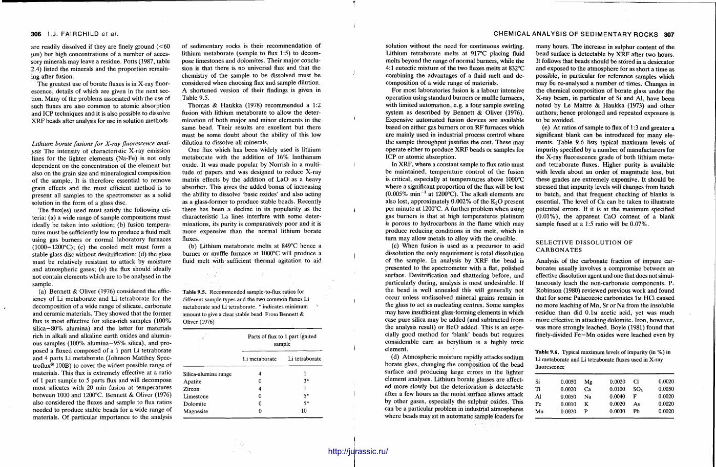
306 I.J. FAIRCHILD ef al.
are readily dissolved if they are finely ground ( < 6 0 um) but high concentrat ions of a number of accessory minerals may leave a residue. Potts (1987, table 2.4) listed the minerals and the proport ion remaining after fusion.
The greatest use of borate fluxes is in X-ray fluorescence, details of which are given in the next section. Many of the problems associated wi th the use of such fluxes are also common to atomic absorpt ion and ICP techniques and it is also possible to dissolve X R F beads after analysis for use in solution methods.
Lithium borate fusions for X-ray fluorescence analysis The intensity of characteristic X-ray emission lines for the lighter e lements (Na-Fe) is not only dependen t on the concentrat ion of the e lement but also on the grain size and mineralogical composit ion of the sample. It is therefore essential to remove grain effects and the most efficient method is to present all samples to the spectrometer as a solid solution in the form of a glass disc.
T h e flux(es) used must satisfy the following criteria: (a) a wide range of sample compositions must ideally be taken into solution; (b) fusion temperatures must be sufficiently low to produce a fluid melt using gas burners or normal laboratory furnaces (1000-1200°C); (c) the cooled melt must form a stable glass disc without devitrification; (d) the glass must be relatively resistant to attack by moisture and atmospheric gases; (e) the flux should ideally not contain elements which are to be analysed in the sample.
(a) Bennet t & Oliver (1976) considered the efficiency of Li me tabora te and Li te t rabora te for the decomposit ion of a wide range of silicate, carbonate and ceramic materials . They showed that the former flux is most effective for silica-rich samples (100% silica—80% alumina) and the latter for materials rich in alkali and alkaline ear th oxides and aluminous samples (100% alumina—95% silica), and proposed a fluxed composed of a 1 part Li te t rabora te and 4 parts Li metabora te (Johnson Mat they Spec-troflux® 100B) to cover the widest possible range of materials. This flux is extremely effective at a ratio of 1 part sample to 5 parts flux and will decompose most silicates with 20 min fusion at tempera tures be tween 1000 and 1200°C. Bennet t & Oliver (1976) also considered the fluxes and sample to flux ratios needed to produce stable beads for a wide range of materials. Of particular importance to the analysis
of sedimentary rocks is their recommendat ion of lithium metabora te (sample to flux 1:5) to decompose limestones and dolomites. Their major conclusion is that there is no universal flux and that the chemistry of the sample to be dissolved must be considered when choosing flux and sample dilution. A shor tened version of their findings is given in Table 9.5.
Thomas & H a u k k a (1978) recommended a 1:2 fusion with lithium metabora te to allow the determination of both major and minor e lements in the same bead. Thei r results are excellent but there must be some doubt about the ability of this low dilution to dissolve all minerals.
O n e flux which has been widely used is lithium metabora te with the addition of 16% lanthanum oxide. It was m a d e popular by Norrish in a multitude of papers and was designed to reduce X-ray matrix effects by the addition of L a O as a heavy absorber . This gives the added bonus of increasing the ability to dissolve 'basic oxides' and also acting as a glass-former to produce stable beads . Recently there has been a decline in its populari ty as the characteristic La lines interfere with some determinat ions, its purity is comparatively poor and it is more expensive than the normal lithium bora te fluxes.
(b) Li thium metabora te melts at 849°C hence a burner or muffle furnace at 1000°C will p roduce a fluid melt with sufficient thermal agitation to aid
Table 9.5. Recommended sample-to-flux ratios for different sample types and the two common fluxes Li metaborate and Li tetraborate. * indicates minimum amount to give a clear stable bead. From Bennett & Oliver (1976)
Parts of flux to 1 part ignited sample
Li metaborate Li tetraborate
Silica-alumina range 4 1 Apatite 0 3* Zircon 4 1 Limestone 0 5* Dolomite 0 5* Magnesite 0 10
11111
CHEMICAL ANALYSIS OF SEDIMENTARY ROCKS 307
solution without the need for continuous swirling. Lithium te t rabora te melts at 917°C placing fluid melts beyond the range of normal burners , while the 4:1 eutectic mixture of the two fluxes melts at 832°C combining the advantages of a fluid melt and decomposition of a wide range of materials.
For most laboratories fusion is a labour intensive operat ion using standard burners or muffle furnaces, with limited automat ion , e.g. a four sample swirling system as described by Bennet t & Oliver (1976). Expensive au tomated fusion devices are available based on ei ther gas burners or on R F furnaces which are mainly used in industrial process control where the sample throughput justifies the cost. These may opera te either to produce X R F beads or samples for ICP or atomic absorption.
In X R F , where a constant sample to flux ratio must be maintained, t empera ture control of t he fusion is critical, especially at tempera tures above 1000°C where a significant propor t ion of the flux will be lost (0 .005% m i n " 1 at 1200°C). The alkali e lements are also lost, approximately 0.002% of the K 2 0 present per minute at 1200°C. A further problem when using gas burners is that at high tempera tures plat inum is porous to hydrocarbons in the flame which may produce reducing conditions in the mel t , which in turn may allow metals to alloy with the crucible.
(c) When fusion is used as a precursor to acid dissolution the only requirement is.total dissolution of the sample. In analysis by X R F the bead is presented to the spectrometer with a flat, polished surface. Devitrification and shattering before, and particularly during, analysis is most undesirable. If the bead is well annealed this will generally not occur unless undissolved mineral grains remain in the glass to act as nucleating centres . Some samples may have insufficient glass-forming elements in which case pure silica may be added (and subtracted from the analysis result) or B e O added. This is an especially good method for 'b lank ' beads but requires considerable care as beryllium is a highly toxic e lement .
(d) Atmospher ic moisture rapidly attacks sodium bora te glass, changing the composit ion of the bead surface and producing large errors in the lighter e lement analyses. Lithium bora te glasses are affected more slowly but the deteriorat ion is detectable after a few hours as the moist surface allows attack by other gases, especially the sulphur oxides. This can be a particular problem in industrial atmospheres where beads may sit in automatic sample loaders for
many hours . The increase in sulphur content of the bead surface is detectable by X R F after two hours . It follows that beads should be stored in a desiccator and exposed to the a tmosphere for as short a t ime as possible, in particular for reference samples which may be re-analysed a number of t imes. Changes in the chemical composit ion of bora te glass under the X-ray beam, in particular of Si and Al , have been noted by Le Maitre & H a u k k a (1973) and other authors ; hence prolonged and repeated exposure is t o b e avoided.
(e) A t ratios of sample to flux of 1:3 and greater a significant blank can be introduced for many elements . Table 9.6 lists typical maximum levels of impurity specified by a number of manufacturers for the X-ray fluorescence grade of both lithium meta-and te t rabora te fluxes. Higher purity is available with levels about an order of magni tude less, but these grades are extremely expensive. It should be stressed that impurity levels will changes from batch to batch, and that frequent checking of blanks is essential. The level of Ca can be taken to illustrate potential errors . If it is at the maximum specified (0 .01%) , the apparent C a O content of a blank sample fused at a 1:5 ratio will be 0 .07%.
S E L E C T I V E D I S S O L U T I O N O F C A R B O N A T E S
Analysis of t he carbonate fraction of impure carbonates usually involves a compromise between an effective dissolution agent and one that does not simultaneously leach the non-carbonate components . P. Robinson (1980) reviewed previous work and found that for some Palaeozoic carbonates 1M HC1 caused no more leaching of M n , Sr o r Na from the insoluble residue than did 0 . 1 M acetic acid, yet was much more effective in attacking dolomite . I ron, however, was more strongly leached. Boyle (1981) found that finely-divided Fe—Mn oxides were leached even by
Table 9.6. Typical maximum levels of impurity (in %) in Li metaborate and Li tetraborate fluxes used in X-ray fluorescence
Si 0.0050 Mg 0.0020 CI 0.0020 Ti 0.0020 Ca 0.0100 s o 3 0.0050 Al 0.0050 Na 0.0040 F 0.0020 Fe 0.0010 K 0.0020 As 0.0020 Mn 0.0020 P 0.0030 Pb 0.0020
http://jurassic.ru/
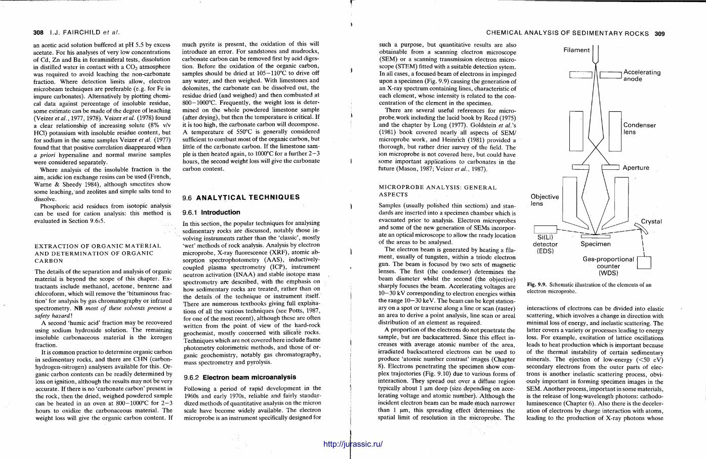
308 I.J. FAIRCHILD ef al.
an acetic acid solution buffered at p H 5.5 by excess aceta te . For his analyses of very low concentrat ions of Cd , Z n and Ba in foraminiferal tests, dissolution in distilled water in contact with a C 0 2 a tmosphere was required to avoid leaching the non-carbonate fraction. Where detection limits allow, electron microbeam techniques are preferable (e.g. for Fe in impure carbonates). Alternatively by plotting chemical data against percentage of insoluble residue, some est imate can be m a d e of the degree of leaching (Veizer etal., 1977, 1978). Veizer et al. (1978) found a clear relationship of increasing solute ( 8 % v/v HC1) potassium with insoluble residue content , but for sodium in the same samples Veizer et al. (1977) found that that positive correlation disappeared when a priori hypersaline and normal marine samples were considered separately.
Where analysis of the insoluble fraction is the aim, acidic ion exchange resins can be used (French, Warne & Sheedy 1984), although smectites show some leaching, and zeolites and simple salts tend to dissolve.
Phosphoric acid residues from isotopic analysis can be used for cation analysis: this method is evaluated in Section 9.6:5.
E X T R A C T I O N O F O R G A N I C M A T E R I A L A N D D E T E R M I N A T I O N O F O R G A N I C C A R B O N
The details of the separation and analysis of organic material is beyond the scope of this chapter . Ex-tractants include methanol , acetone, benzene and chloroform, which will remove the 'bi tuminous fract ion' for analysis by gas chromatography or infrared spectrometry. NB most of these solvents present a safety hazard!
A second 'humic acid' fraction may be recovered using sodium hydroxide solution. T h e remaining insoluble carbonaceous material is the kerogen fraction.
It is common practice to determine organic carbon in sedimentary rocks, and there are C H N (carbon-hydrogen-nitrogen) analysers available for this. Organic carbon contents can be readily determined by loss on ignition, al though the results may not be very accurate. If there is no 'carbonate carbon ' present in the rock, then the dried, weighed powdered sample can be heated in an oven at 800-1000°C for 2 - 3 hours to oxidize the carbonaceous material . The weight loss will give the organic carbon content . If
much pyrite is present , the oxidation of this will introduce an error . For sandstones and mudrocks , carbonate carbon can be removed first by acid digestion. Before the oxidation of the organic carbon, samples should be dried at 105—110°C to drive off any water , and then weighed. With l imestones and dolomites , the carbonate can be dissolved out , the residue dried (and weighed) and then combusted at 800-1000°C. Frequent ly , the weight loss is determined on the whole powdered l imestone sample (after drying), but then the tempera ture is critical. If it is too high, the carbonate carbon will decompose . A tempera ture of 550°C is generally considered sufficient to combust most of the organic carbon, but little of the carbonate carbon. If the l imestone sample is then heated again, to 1000°C for a further 2—3 hours , the second weight loss will give the carbonate carbon content .
9.6 A N A L Y T I C A L T E C H N I Q U E S
9.6.1 Introduction
In this section, the popular techniques for analysing sedimentary rocks are discussed, notably those involving instruments ra ther than the 'classic', mostly 'wet ' methods of rock analysis. Analysis by electron microprobe , X-ray fluorescence ( X R F ) , atomic absorption spectrophotometry ( A A S ) , inductively-coupled plasma spectrometry ( ICP) , instrument neut ron activation ( I N A A ) and stable isotope mass spectrometry are described, with the emphasis on how sedimentary rocks are t reated, ra ther than on the details of the technique or instrument itself. The re are numerous textbooks giving full explanations of all the various techniques (see Potts , 1987, for one of the most recent ) , al though these are often written from the point of view of the hard-rock geochemist , mostly concerned with silicate rocks. Techniques which are not covered here include flame photometry coiorimetric methods , and those of organic geochemistry, notably gas chromatography, mass spectrometry and pyrolysis.
9.6.2 Electron beam microanalysis
Following a period of rapid development in the 1960s and early 1970s, reliable and fairly standardized methods of quanti tat ive analysis on the micron scale have become widely available. The electron microprobe is an instrument specifically designed for
CHEMICAL ANALYSIS OF SEDIMENTARY ROCKS 309
such a purpose , but quanti tat ive results are also obtainable from a scanning electron microscope (SEM) or a scanning transmission electron microscope (STEM) fitted with a suitable detection sytem. In all cases, a focused beam of electrons in impinged upon a specimen (Fig. 9.9) causing the generat ion of an X-ray spectrum containing lines, characteristic of each e lement , whose intensity is related to the concentrat ion of the e lement in the specimen.
There are several useful references for microprobe, work including the lucid book by Reed (1975) and the chapter by Long (1977). Goldstein et a/. 's (1981) book covered nearly all aspects of SEM/ microprobe work, and Heinrich (1981) provided a thorough, but ra ther drier survey of the field. The ion microprobe is not covered here , but could have some important applications to carbonates in the future (Mason, 1987; Veizer etal., 1987).
M I C R O P R O B E A N A L Y S I S : G E N E R A L A S P E C T S
Samples (usually polished thin sections) and standards are inserted into a specimen chamber which is evacuated prior to analysis. Electron microprobes and some of the new generat ion of SEMs incorporate an optical microscope to allow the ready location of the areas to be analysed.
The electron beam is genera ted by heating a filament , usually of tungsten, within a tr iode electron gun. The beam is focused by two sets of magnetic lenses. The first ( the condenser) determines the beam diameter whilst the second (the objective) sharply focuses the beam. Accelerating voltages are 10—30 kV corresponding to electron energies within the range 10—30 keV. The beam can be kept stationary on a spot or traverse along a line or scan (raster) an area to derive a point analysis, line scan or areal distribution of an element as required.
A proport ion of the electrons do not penet ra te the sample, but are backscattered. Since this effect increases with average atomic number of the area , i r radiated backscat tered electrons can be used to produce 'a tomic number contrast ' images (Chapter 8). Electrons penetrat ing the specimen show complex trajectories (Fig. 9.10) due to various forms of interaction. They spread out qVer a diffuse region typically about 1 um deep (size depending on accelerating voltage and atomic number ) . Al though the incident electron beam can be made m u c h narrower than 1 um, this spreading effect determines the spatial limit of resolution in the microprobe. The
Filament
Accelerating anode
Objective lens
Gas-proportional counter (WDS)
Fig. 9.9. Schematic illustration of the elements of an electron microprobe.
interactions of electrons can be divided into elastic scattering, which involves a change in direction with minimal loss of energy, and inelastic scattering. The latter covers a variety or processes leading to energy loss. For example, excitation of lattice oscillations leads to heat product ion which is important because of the thermal instability of certain sedimentary minerals. The ejection of low-energy ( < 5 0 eV) secondary electrons from the outer parts of electrons is another inelastic scattering process, obviously important in forming specimen images in the S E M . Ano the r process, important in some materials , is the release of long-wavelength photons: cathodoluminescence (Chapter 6) . Also there is the deceleration of electrons by charge interaction with a toms , leading to the production of X-ray photons whose
http://jurassic.ru/
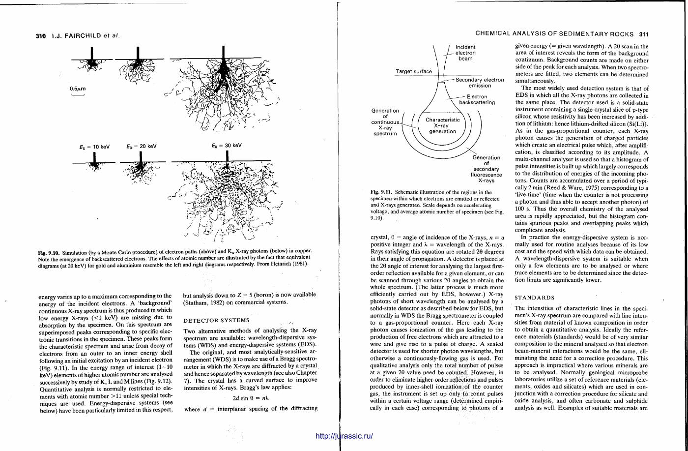
310 I.J. FAIRCHILD ET AL.
E0 = 10 keV f 0 = 20 keV E0 = 30 keV
Fig. 9.10. Simulation (by a Monte Carlo procedure) of electron paths (above) and K„ X-ray photons (below) in copper. Note the emergence of backscattered electrons. The effects of atomic number are illustrated by the fact that equivalent diagrams (at 20 keV) for gold and aluminium resemble the left and right diagrams respectively. From Heinrich (1981).
energy varies u p to a maximum corresponding to t he energy of the incident electrons. A 'background ' cont inuous X-ray spectrum is thus produced in which low energy X-rays ( < 1 keV) are missing due to absorption by the specimen. O n this spectrum are superimposed peaks corresponding to specific electronic transitions in the specimen. These peaks form the characteristic spectrum and arise from decay of electrons from an outer to an inner energy shell following an initial excitation by an incident electron (Fig. 9.11). In the energy range of interest (1—10 keV) elements of higher atomic numbeT a re analysed successively by study of K, L and M lines (Fig. 9.12). Quanti tat ive analysis is normally restricted to elements with a tomic number > 1 1 unless special techniques are used. Energy-dispersive systems (see below) have been particularly limited in this respect,
but analysis down to Z = 5 (boron) is now available (Sta tham, 1982) on commercial systems.
D E T E C T O R S Y S T E M S
Two alternative methods of analysing the X-ray spectrum are available: wavelength-dispersive systems ( W D S ) and energy-dispersive systems ( E D S ) .
The original, and most analytically-sensitive arrangement ( W D S ) is t o m a k e use of a Bragg spectrometer in which the X-rays are diffracted by a crystal and hence separated by wavelength (see also Chap te r 7) . The crystal has a curved surface to improve intensities of X-rays. Bragg 's law applies:
2d sin 9 = rik
where d — interplanar spacing of the diffracting
CHEMICAL ANALYSIS OF SEDIMENTARY ROCKS 311
secondary fluorescence
X-rays
Fig. 9.11. Schematic illustration of the regions in the specimen within which electrons are emitted or reflected and X-rays generated. Scale depends on accelerating voltage, and average atomic number of specimen (see Fig. 9.10).
crystal, 0 = angle of incidence of the X-rays, n = a positive integer and X = wavelength of the X-rays. Rays satisfying this equat ion are ro ta ted 28 degrees in their angle of propagat ion. A detector is placed at the 26 angle of interest for analysing the largest first-order reflection available for a given e lement , or can be scanned through various 26 angles to obtain the whole spectrum. (The latter process is much more efficiently carried out by E D S , however . ) X-ray photons of short wavelength can be analysed by a solid-state detector as described below for E D S , but normally in W D S the Bragg spectrometer is coupled to a gas-proportional counter . H e r e each X-ray photon causes ionization of the gas leading to the product ion of free electrons which are at tracted to a wire and give rise to a pulse of charge. A sealed detector is used for shorter photon wavelengths, but otherwise a continuously-flowing gas is used. For qualitative analysis only the total number of pulses at a given 26 value need be counted . However , in order to eliminate higher-order reflections and pulses produced by inner-shell ionization of the counter gas, the instrument is set up only to count pulses within a certain voltage range (determined empirically in each case) corresponding to photons of a
given energy ( = given wavelength) . A 26 scan in the area of interest reveals the form of the background cont inuum. Background counts are m a d e on either side of the peak for each analysis. When two spectrometers are fitted, two elements can be determined simultaneously.
The most widely used detection system is that of E D S in which all the X-ray photons are collected in the same place. T h e detector used is a solid-state instrument containing a single-crystal slice of p-type silicon whose resistivity has been increased by addition of lithium: hence lithium-drifted silicon (Si(Li)). As in the gas-proportional counter , each X-ray photon causes the generat ion of charged particles which create an electrical pulse which, after amplification, is classified according to its ampli tude. A multi-channel analyser is used so that a histogram of pulse intensities is built up which largely corresponds to the distribution of energies of the incoming photons . Counts are accumulated over a period of typically 2 min (Reed & Ware , 1975) corresponding to a ' l ive-time' (time when the counter is not processing a photon and thus able to accept another photon) of 100 s. Thus t he overall chemistry of the analysed area is rapidly appreciated, but the histogram contains spurious peaks and overlapping peaks which complicate analysis.
In practice the energy-dispersive system is normally used for rout ine analyses because of its low cost and the speed with which data can be obtained. A wavelength-dispersive system is suitable when only a few elements are to be analysed or where trace elements are to be determined since the detection limits are significantly lower.
S T A N D A R D S
The intensities of characteristic lines in the specimen ' s X-ray spectrum are compared with line intensities from material of known composition in order to obtain a quanti tat ive analysis. Ideally the reference materials (standards) would be of very similar composition to the mineral analysed so that electron beam-minera l interactions would b e the same, eliminating the need for a correction procedure . This approach is impractical where various minerals are to be analysed. Normally geological microprobe laboratories utilize a set of reference materials (elements , oxides and silicates) which are used in conjunction with a correction procedure for silicate and oxide analysis, and often carbonate and sulphide analysis as well. Examples of suitable materials are
http://jurassic.ru/
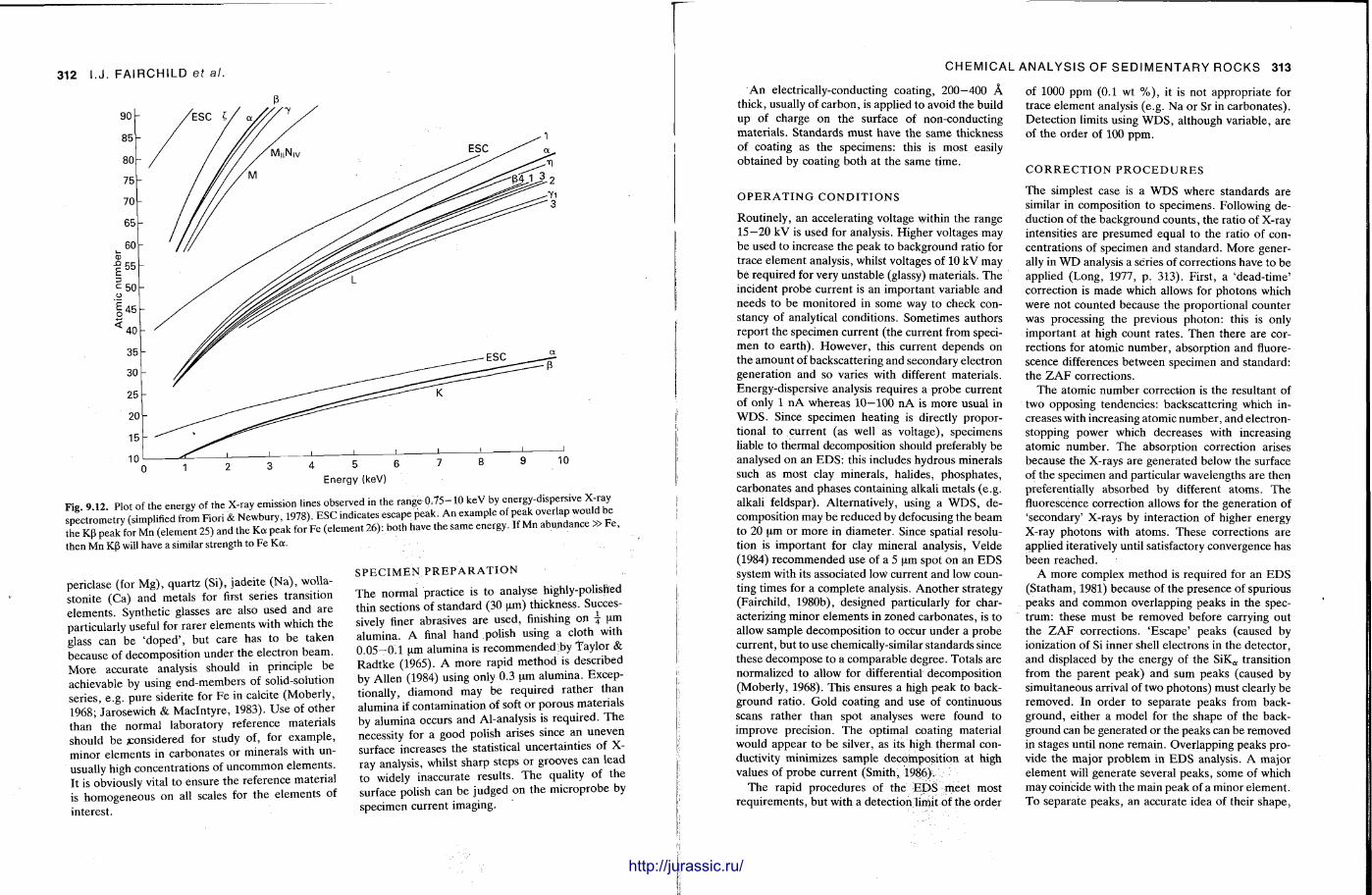
312 I.J. FAIRCHILD ef al.
0 1 2 3 4 5 6 7 8 9 10 Energy (keV)
Fig. 9.12. Plot of the energy of the X-ray emission lines observed in the range 0,75-10 keV by energy-dispersive X-ray spectrometry (simplified from Fiori & Newbury, 1978). ESC indicates escape peak. An example of peak overlap would be the KfJ peak for Mn (element 25) and the Ka peak for Fe (element 26): both have the same energy. If Mn abundance » Fe, then Mn K(5 will have a similar strength to Fe Ka.
periclase (for M g ) , quartz (Si), jadei te (Na) , wolla-stonite (Ca) and metals for first series transition elements . Synthetic glasses are also used and are particularly useful for rarer elements with which the glass can be ' doped ' , but care has to b e taken because of decomposit ion unde r the electron beam. M o r e accurate analysis should in principle be achievable by using end-members of solid-solution series, e.g. pure siderite for Fe in calcite (Moberly, 1968; Jarosewich & Macln ty re , 1983). Use of other than the normal laboratory reference materials should be ^considered for study of, for example , minor e lements in carbonates or minerals with unusually high concentrat ions of uncommon elements . It is obviously vital to ensure the reference material is homogeneous on all scales for the e lements of interest .
S P E C I M E N P R E P A R A T I O N
T h e normal practice is to analyse highly-polished thin sections of s tandard (30 um) thickness. Successively finer abrasives are used, finishing on \ um alumina. A final hand polish using a cloth with 0.05—0.1 um alumina is r ecommended :by Taylor & R a d t k e (1965). A more rapid method is described by Allen (1984) using only 0.3 um alumina. Exceptionally, d iamond may be required ra ther than alumina if contaminat ion of soft or porous materials by alumina occurs and Al-analysis is required. T h e necessity for a good polish arises since an uneven surface increases the statistical uncertainties of X-ray analysis, whilst sharp steps or grooves can lead to widely inaccurate results. T h e quality of the surface polish can be judged on the microprobe by specimen current imaging.
CHEMICAL ANALYSIS OF SEDIMENTARY ROCKS 313
A n electrically-conducting coating, 2 0 0 - 4 0 0 A thick, usually of carbon, is applied to avoid the build up of charge on the surface of non-conducting materials . Standards must have the same thickness of coating as the specimens: this is most easily obtained by coating both at the same t ime.
O P E R A T I N G C O N D I T I O N S
Routinely, an accelerating voltage within the range 15—20 kV is used for analysis. Higher voltages may be used to increase the peak to background ratio for trace element analysis, whilst voltages of 10 kV may be required for very unstable (glassy) materials. The incident p robe current is an important variable and needs to be moni tored in some way to check constancy of analytical condit ions. Sometimes authors report the specimen current (the current from specimen to ea r th ) . However , this current depends on the amount of backscattering and secondary electron generat ion and so varies with different materials. Energy-dispersive analysis requires a probe current of only 1 n A whereas 1 0 - 1 0 0 n A is more usual in W D S . Since specimen heating is directly proportional to current (as well as voltage), specimens liable to thermal decomposition should preferably be analysed on an E D S : this includes hydrous minerals such as most clay minerals , halides, phosphates , carbonates and phases containing alkali metals (e .g. alkali feldspar). Alternatively, using a W D S , decomposit ion may be reduced by defocusing the beam to 20 (im or more in diameter . Since spatial resolution is important for clay mineral analysis, Velde (1984) recommended use of a 5 um spot on an E D S system with its associated low current and low counting t imes for a complete analysis. Ano the r strategy (Fairchild, 1980b), designed particularly for characterizing minor e lements in zoned carbonates , is to allow sample decomposit ion to occur under a probe current , but to use chemically-similar s tandards since these decompose to a comparable degree. Totals are normalized to allow for differential decomposit ion (Moberly, 1968). This ensures a high peak to background ratio. Gold coating and use of continuous scans ra ther than spot analyses were found to improve precision. T h e optimal coating material would appear to be silver, as its high thermal conductivity minimizes sample decomposit ion at high values of probe current (Smith, 1986).
The rapid procedures of the E D S meet most requirements , but with a detection limit of the order
of 1000 ppm (0.1 wt % ) , it is not appropria te for trace element analysis (e.g. Na or Sr in carbonates) . Detect ion limits using W D S , although variable, are of the order of 100 ppm.
C O R R E C T I O N P R O C E D U R E S
The simplest case is a W D S where s tandards are similar in composition to specimens. Following deduction of the background counts , the ratio of X-ray intensities are presumed equal to the ratio of con^ centrat ions of specimen and s tandard. More generally in W D analysis a series of corrections have to be applied (Long, 1977, p . 313). First, a 'dead-t ime 7
correction is made which allows for photons which were not counted because the proport ional counter was processing the previous photon: this is only important at high count rates . Then there are corrections for atomic number , absorption and fluorescence differences between specimen and standard: the Z A F corrections.
T h e atomic number correction is the resultant of two opposing tendencies: backscattering which increases with increasing atomic number , and electron-stopping power which decreases with increasing atomic number . The absorption correction arises because the X-rays are generated below the surface of the specimen and particular wavelengths are then preferentially absorbed by different a toms. T h e fluorescence correction allows for the generat ion of 'secondary' X-rays by interaction of higher energy X-ray photons with a toms. These corrections are applied iteratively until satisfactory convergence has been reached.
A more complex method is required for an E D S (Statham, 1981) because of the presence of spurious peaks and common overlapping peaks in the spect rum: these must be removed before carrying out the Z A F corrections. 'Escape ' peaks (caused by ionization of Si inner shell electrons in the detector , and displaced by the energy of the S i K a transition from the parent peak) and sum peaks (caused by simultaneous arrival of two photons) must clearly be removed. In order to separate peaks from background, either a model for the shape of the background can be generated or the peaks can be removed in stages until none remain . Overlapping peaks provide t he major p roblem in E D S analysis. A major e lement will generate several peaks , some of which may coincide with the main peak of a minor element . T o separate peaks , an accurate idea of their shape,
http://jurassic.ru/
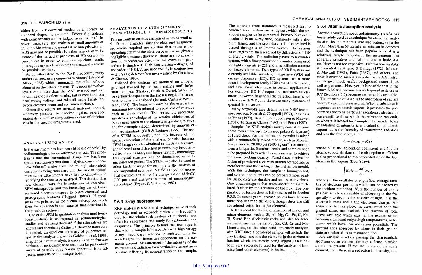
314 I.J. FAIRCHILD et al.
either from a theoretical model , o r a ' l ibrary' of standard shapes, is required. Potential problems with peak overlap can be judged from Fig. 9.12. In severe cases (e.g. the analysis of small amounts of Fe in an Mn minera l ) , quanti tat ive analysis with an E D S may not be possible. It is thus important to be aware of the particular problems of E D correction procedures in o rde r to el iminate spurious results al though many modern systems automatically advise on possible overlaps.
As an alternative to the Z A F procedure , many authors correct using empirical 'a-factors ' (Bence & A l b e e , 1968) which summarize the effect of one element on the others present . This process involves less computat ion than the Z A F method and can obtain near-equivalent results, but is specific t o one accelerating voltage and take-off angle (angle between electron b e a m and specimen surface).
General ly, results for unusual materials should, wherever possible, be checked against reference materials of similar composit ion in case of deficiencies in the specific p rog ramme used.
A N A L i s i a U S I N G AN S E M In the past there has been very little use of SEMs by sedimentologists for quanti tat ive analysis. T h e problem is that the pre-eminent design aim has been spatial resolution rather than analytical convenience. Low take-off angles have led to high absorpt ion corrections being necessary and the lack of optical microscope at tachments have led to difficulties in specifying the area to be analysed. This situation has now changed with the introduction of combined SEM-microprobes and the increasing use of back-scattered electron imagery to relate chemical and petrographic features (Hugget t , 1984a). If specimens are polished as for normal microprobe work then the situation is the same as that described in the previous sections.
Use of the S E M in qualitative analysis (and hence identification) is widespread in sedimentological studies and is striaghtforward if the alternatives are known and chemically distinct. Otherwise more care is needed: an excellent summary of guidelines for qualitative analysis is given in Goldstein et al. (1981, chapter 6) . Often analysis is under taken on fracture surfaces of rock chips: here one must be particularly aware of possible stray X-rays generated from adjacent minerals or the sample holder .
A N A L Y S I S U S I N G A S T E M ( S C A N N I N G T R A N S M I S S I O N E L E C T R O N M I C R O S C O P E )
This instrument enables analysis of areas as small as 5—10 nm in diameter , since the electron-transparent specimens required are so thin that there is no spreading effect of the electron b e a m . Also , given a negligible specimen thickness, there a re n o absorption o r fluorescence effects so the correction procedure is simplified. High accelerating voltages, of the order of 100 kV, are used usually in conjunction with a Si(Li) detector (see review article by Goodhew & Chesco, 1980).
Polished thin sections are mounted on a metal grid and thinned by ion-beam milling until holes start to appear (Phakey, Curtis & Oer te l , 1972). T o b e certain that specimen thickness is negligible, areas next to holes are analysed (Ireland, Curtis & White-man , 1983). T h e beam size must be above a certain minimum for each mineral to avoid loss of volatiles such as alkali metals . T h e correction procedure involves a knowledge of the relative efficiencies of X-ray generat ion of the e lement in quest ion relative t o , for example silicon, de termined by analysis of» thinned standards (Cliff & Lorimer , 1975). T h e use of a S T E M is powerful, not only because of the spatial resolution of the analysis, but also because T E M images can be obtained to illustrate textures , and selected-area diffraction pat terns may be obtained from grains analysed: hence texture , mineralogy and crystal structure can be determined on sub-micron-sized grains. T h e S T E M can also be used in other kinds of ways: for example in the analysis of -fine suspended sediment , S T E M analysis of individual particles can allow the interpretat ion of 'bulk ' (100 um area) analyses in te rms of mineralogical percentages (Bryant & Williams, 1982).
9.6.3 X-ray f luorescence X R F analysis is a s tandard technique in hard-rock petrology and in soft-rock circles it is frequently used for the whole-rock analysis of mudrocks , less often for sandstones and rarely for carbonates and evapori tes. T h e principle behind this technique is that when a sample is bombarded with high energy X-rays, secondary radiation is emit ted, with the wavelengths and intensities dependent on the elements present . Measurement of the intensity of the characteristic radiation for a particular e lement gives a value reflecting its concentrat ion in the sample.
CHEMICAL ANALYSIS OF SEDIMENTARY ROCKS 315
T h e emission from standards is measured first to produce a calibration curve, against which the unknown samples an be compared . Primary X-rays are produced in an X-ray tube , commonly with a rhodium target , and the secondary radiation emitted is passed through a collimator system. The various wavelengths are then resolved by diffraction off LiF or P E T crystals. T h e radiation passes to a counter system, with a flow proport ional counter being used for light elements ( < 2 2 ) and a scintillation counter for heavy elements . Two types of X R F system are currently available: wavelength dispersive (WD) and energy dispersive ( E D ) . E D systems are a more recent development (early 1970s) than the W D units, and have some advantages in certain applications. For example , E D is cheaper and measures all elements , however , in general the detection limit is not as low as with W D , and there are many instances of spectral line overlap.
Many textbooks give details of the X R F technique ; see, e.g. Norrish & Chappell (1977), Jenkins & de Vries (1970), Bert in (1975), Johnson & Maxwell (1981), Ter t ian & Claisse (1982) and Potts (1987).
Samples for X R F analysis mostly consist of powdered rocks made up into pressed pellets (briquettes) or fused discs. For the pellets, the powder is mixed with a commercially mixed binder , such as Mowoil , and pressed to 20,000 psi (1400 kg c m - 2 ) or more to form a br iquet te . S tandard rocks and samples need to be prepared in exactly the same manner to achieve the same packing density. Fused discs involve the fusion of powdered rock with lithium te t raborate or metabora te and the casting of the melt into a mould. With this technique, the sample is homogenized, and synthetic s tandards can be prepared more readily. Also, discs are durable and can be many t imes. O n e disadvantage is that trace constituents are diluted further by the addition of the flux. The preparat ion of fusion discs is fully discussed in Section 9.5.3. In recent years , pressed pellets have become more popular than the disc al though discs are still considered bet ter for major e lements .
X R F is ideal for the determinat ion of major and minor e lements , such as Si, Al , Mg , Ca , F e , K, N a , Ti , S and P in siliciclastic rocks and also for trace e lements , such as metals Pb , Z n , Cd, Cr and Mn. Limestones , on the o ther hand, are rarely analysed with X R F since a powdered sample will include the clay fraction, and it is t he e lements in the carbonate fraction which are mostly being sought. X R F has been very successfully used for the analysis of bromine (and other elements) in halite.
9.6.4 Atomic absorpt ion analysis
Atomic absorption spectrophotometry (AAS) has been widely used as a technique for elemental analysis of rocks and minerals , and also waters , since the 1960s. More than 50 useful elements can be detected and the technique has been popular since it is a relatively simple procedure , the instruments are generally sensitive and reliable, and a basic A A machines is not too expensive. Information o n A A S is presented by Angino & Billings (1972), Johnson & Maxwell (1981), Potts (1987), and others , and most instruction manuals supplied with A A instruments give much useful background material , as well as guidance. However , it is possible that in the future A A S will become less widespread in its use as ICP (Section 9.6.5) becomes more readily available.
T h e principle of A A S is t he absorpt ion of radiant energy by ground state a toms. When a substance is dispersed as an atomic vapour , it possesses the property of absorbing particular radiations, identical in wavelength to those which the substance can emit , as when it is hea ted for example . If a parallel beam of radiation of intensity I0 is incident on an atomic vapour , Iv is the intensity of transmitted radiation and v is the frequency, then
Iv = I0exp(-Kvl)
where Kv is the absorption coefficient and / is the atomic vapour thickness. T h e absorption coefficient is also proport ional t o the concentrat ion of t he free a toms in the vapour (Beer ' s law):
Kvdv = —Nvf mc
w h e r e / i s the oscillator strength (i .e . average number of electrons pe r a tom which can be excited by the incident radiat ion) , Nv is the number of atoms per c m 3 which are capable of absorbing in the frequently v to dv, c is the velocity of light, m is the electronic mass and e the electronic charge. For absorption to take place, the atoms must be in the ground state , not excited. T h e fraction of total a toms available which exist in the excited stated becomes significant only at high tempera tures , or for a toms which have low ionization potentials. The spectral lines absorbed by a toms in their ground state are referred to as resonance lines.
A A analysis involves passing the characteristic spectrum of an element through a flame in which a toms a re present . If t he a toms are of the same element , then there is a reduction in intensity, due
iinmiiiiiiiiiiiiiiiiii] http://jurassic.ru/
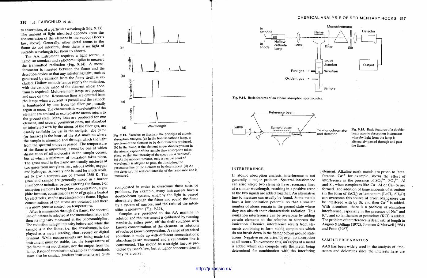
316 I.J. FAIRCHILD ef al.
to absorpt ion, of a particular wavelength (Fig. 9.13). The amount of light absorbed depends upon the concentrat ion of the e lement in the vapour (Beer ' s law, above) . General ly , other metal a toms in the flame do not interfere, since there is no light of suitable wavelength for them to absorb.
T h e A A inst rument requires a light source, a flame, an atomizer and a photomult ipl ier to measure the transmitted raditat ion (Fig. 9.14). A monochromator is inserted between the flame and the detection device so that any interfering light, such as generated by emission from the flame itself, is excluded. Hollow-cathode lamps supply the radiat ion, with the cathode m a d e of the e lement whose spect rum is required. Mult i-element lamps are popular , and save on t ime. Resonance lines are emit ted from the lamps when a current is passed and the cathode is bombarded by ions from the filler gas, usually argon o r neon . T h e characteristic wavelengths of the e lement are emit ted as excited-state a toms re turn to the ground state . Many lines a re produced for one e lement , and several prominent ones , not absorbed or interfered with by the atoms of t he filler gas, a re usually available for use in the analysis. T h e flame (or furnace) is the hear t of the A A machine where the sample is atomized and through which the light from the spectral source is passed. The tempera ture of the flame is impor tant ; it must be one at which dissociation of all molecules in the sample occurs, but at which a minimum of ionization takes place. T h e gases used in the flame are usually mixtures of two gases from acetylene, air, nitrous oxide, oxygen and hydrogen. Air-acetylene is used for much work, set to give a t empera tu re of a round 2350 K. T h e gases and sample are generally mixed in a bu rne r chamber or nebulizer before entering the flame. For analysing elements in very low concentrat ion, a graphite furnace, consisting of a tube of graphite heated by electrodes, can be used instead of a flame. Higher concentrat ions of the atoms are obtained and there is a more precise control on tempera ture .
After transmission through the flame, the spectral line of interest is selected at the monochromator and then its intensity measured at the photomult ipl ier . The reduction in light intensity before and while the sample is in the flame, i .e. the absorbance , is displayed as a meter reading, chart record or digital pr intout . While measurements are being made the instrument must be stable, i.e. the t empera ture of the flame must not change, nor the output from the lamp. Ra tes of atomization of samples and standards must also be similar. Modern instruments are quite
(b)
(rj) Wavelength
Fig. 9.13. Sketches to illustrate the principle of atomic absorption analysis, (a) In the hollow-cathode lamp, a spectrum of the element to be determined is produced. (b) In the flame, if the element in question is present in the atomic vapour of the sample then absorption takes place, so that the intensity of the spectrum is 'reduced'. (c) At the monochromator, only a narrow band of wavelength is allo.wed to pass, that including the resonance line of the element to be determined, (d) At the detector, the reduced intensity of the resonance line is measured.
complicated in order to overcome these sorts of problems. For example , many instruments have a double-beam system, whereby the light is passed alternately through the flame and round the flame by a system of mirrors , and the ratio of the intensities is measured (Fig. 9.15).
Samples are presented to the A A machine in solution and the instrument is calibrated by running s tandards , ei ther pu re , off-the-shelf solutions with known concentrat ions of the e lement , or solutions of rocks of known composit ion. A range of s tandard solutions is made u p with different concentra t ions; absorbances are measured and a calibration line is constructed. This should be a straight l ine, as predicted by Beer ' s law, but at higher concentrat ions it may be a curve.
CHEMICAL ANALYSIS OF SEDIMENTARY ROCKS 317
to
cathode
to anode
Monochromator
Hollow cathode lamp
Flame
Lens
Fuel gas —• =={
Oxidant gas —» 1
CD
Filter
Cloud chamber
Nebulizer
Sample
Fig. 9.14. Basic features of an atomic absorption spectrometer.
Detector
Slit
Output
Reference beam
Sample beam
Flame" To monochromator and detector
Fig. 9.15. Basic features of a double-beam atomic absorption instrument whereby light from the lamp is alternately passed through and past the flame.
I N T E R F E R E N C E
In atomic absorption analysis, interference is not generally a major problem. Spectral interference can arise where two e lements have resonance lines at a similar wavelength, resulting in a positive error as the two signals are added together. A n alternative line to measure can usually be found. Some metals have a low ionization potential so that a smaller number of a toms remain in the ground state where they can absorb their characteristic radiation. This ionization interference can be overcome by adding certain e lements to the solution to suppress the ionization. Chemical interference results from elements combining to form stable compounds which do not break down in the flame to form ground state a toms. Negative errors arise, or even no absorption at all occurs. T o overcome this, an excess of a metal is added which can compete with t h e metal being determined for combinat ion with; the interfering
element . Alkal ine ear th metals are prone to interference. C a 2 + for example , shows the effect of interference in the presence of S 0 4
2 ~ , P 0 4
3 ~ , Al and Si, when complexes like Ca—Al or Ca—Si are formed. The addition of large amounts of s trontium (in the form of SrCl 2 ) or lanthanum ( L a C l 3 . 6H z O) can overcome this source of error . Manganese can be interfered with by Si, and then C a 2 + is added. With s t ront ium, there is a problem of ionization interference, especially in the presence of N a + and K + , and so l an thanum or potassium (KC1) is added. The problem of interference is dealt with at length in Angino & Billings (1972), Johnson & Maxwell (1981) and Potts (1987).
S A M P L E P R E P A R A T I O N
A A S has been widely used in the analysis of limestones and dolomites since the interests here are
http://jurassic.ru/
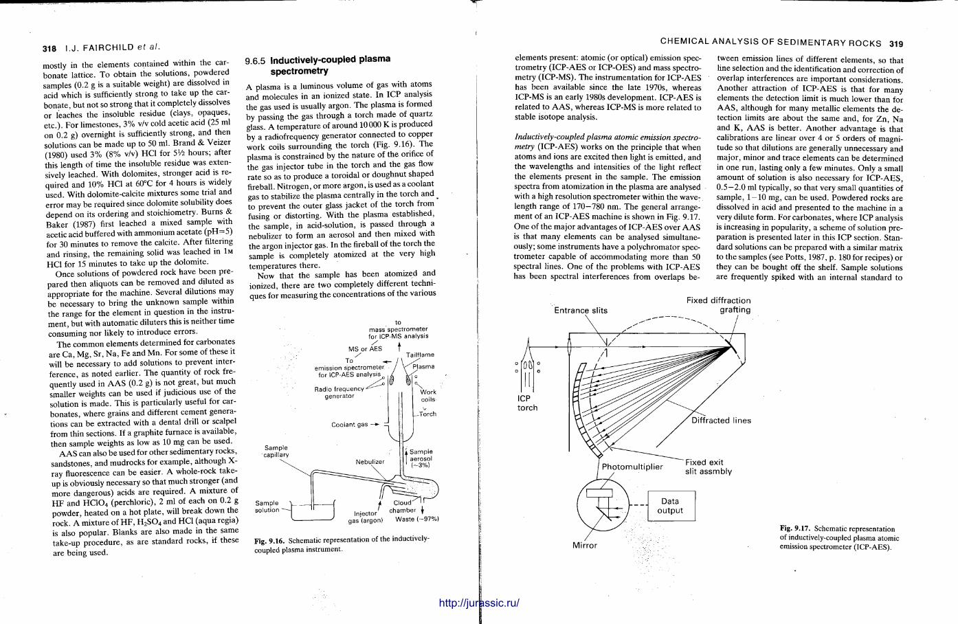
318 I.J. FAIRCHILD ef al.
mostly in the elements contained within the carbonate lattice. T o obtain the solutions, powdered samples (0.2 g is a suitable weight) are dissolved in acid which is sufficiently strong to t ake up the carbona te , but not so s trong that it completely dissolves or leaches the insoluble residue (clays, opaques , e tc . ) . For l imestones, 3 % v/v cold acetic acid (25 ml on 0.2 g) overnight is sufficiently strong, and then solutions can be made up to 50 ml. Brand & Veizer (1980) used 3 % ( 8 % v/v) HC1 for 5Vi hours ; after this length of t ime the insoluble residue was extensively leached. With dolomites , stronger acid is required and 10% HC1 at 60°C for 4 hours is widely used. With dolomite-calcite mixtures some trial and error may be required since dolomite solubility does depend on its ordering and stoichiometry. Burns & Baker (1987) first leached a mixed sample with acetic acid buffered with ammonium acetate ( p H = 5 ) for 30 minutes to remove the calcite. After filtering and rinsing, the remaining solid was leached in 1M HC1 for 15 minutes to take up the dolomite .
Once solutions of powdered rock have been prepared then aliquots can be removed and diluted as appropr ia te for t he machine. Several dilutions may be necessary to bring the unknown sample within the range for the e lement in question in the instrumen t , bu t with automat ic diluters this is nei ther t ime consuming nor likely to introduce errors .
The common elements determined for carbonates are Ca, Mg, Sr, N a , Fe and Mn. For some of these it will be necessary to add solutions to prevent interference, as noted earlier. T h e quantity of rock frequently used in A A S (0.2 g) is not great , bu t much smaller weights can be used if judicious use of the solution is m a d e . This is particularly useful for carbona tes , where grains and different cement generations can be extracted with a dental drill or scalpel from thin sections. If a graphite furnace is available, then sample weights as low as 10 mg can be used.
A A S can also be used for o ther sedimentary rocks, sandstones, and mudrocks for example , al though X-ray fluorescence can b e easier. A whole-rock take-u p is obviously necessary so that much stronger (and more dangerous) acids are required. A mixture of H F and H C 1 0 4 (perchloric), 2 ml of each on 0.2 g powder , heated on a hot plate , will break down the rock. A mixture of H F , H 2 S 0 4 and HC1 (aqua regia) is also popular . Blanks a re also m a d e in the same take-up procedure , as a re s tandard rocks , if these are being used.
9.6.5 Inductively-coupled plasma spectrometry
A plasma is a luminous volume of gas with a toms and molecules in an ionized state. In ICP analysis the gas used is usually argon. The plasma is formed by passing the gas through a torch m a d e of quar tz glass. A tempera ture of around 10000 K is produced by a radiofrequency generator connected to copper work coils surrounding the torch (Fig. 9.16). T h e plasma is constrained by the na ture of the orifice of the gas injector tube in the torch and the gas flow rate so as to produce a toroidal or doughnut shaped fireball. Ni t rogen, or more argon, is used as a coolant gas to stabilize the plasma centrally in the torch and to prevent the outer glass jacket of the torch from fusing or distorting. With the plasma established, the sample , in acid-solution, is passed through a nebulizer to form an aerosol and then mixed with the argon injector gas. In the fireball of the torch the sample is completely atomized at the very high tempera tures there .
Now that the sample has been atomized and ionized, there a re two completely different techniques for measuring the concentrat ions of the various
to mass spectrometer for ICP-MS analysis
t Tailflame
MS or AES /
To emission spectrometer
for ICP-AES analysis
Radio frequency generator
Sample capillary
Sample solution
Cloud 1 1
chamber \ Waste (-97%)
Fig. 9.16. Schematic representation of the inductively-coupled plasma instrument.
CHEMICAL ANALYSIS OF SEDIMENTARY ROCKS 319
elements present: a tomic (or optical) emission spect rometry ( ICP-AES or ICP-OES) and mass spectrometry ( ICP-MS) . T h e inst rumentat ion for I C P - A E S has been available since the late 1970s, whereas ICP-MS is an early 1980s development . ICP-AES is related to A A S , whereas ICP-MS is more related to stable isotope analysis.
Inductively-coupled plasma atomic emission spectrometry ( ICP-AES) works on the principle that when atoms and ions are excited then light is emit ted, and the wavelengths and intensities of t he light reflect the elements present in the sample. The emission spectra from atomization in the plasma are analysed with a high resolution spectrometer within the wavelength range of 170—780 nm. The general arrangement of an I C P - A E S machine is shown in Fig. 9.17. O n e of the major advantages of ICP-AES over A A S is that many elements can be analysed simultaneously; some instruments have a polychromator spect rometer capable of accommodat ing m o r e than 50 spectral lines. O n e of the problems with ICP-AES has been spectral interferences from overlaps be
tween emission lines of different e lements , so that line selection and the identification and correction of overlap interferences are important considerations. Ano the r attraction of I C P - A E S is that for many elements the detection limit is much lower than for A A S , al though for many metallic elements the detection limits are about the same and, for Z n , Na and K, A A S is bet ter . Ano the r advantage is tha t calibrations are linear over 4 or 5 orders of magnitude so that dilutions are generally unnecessary and major , minor and trace elements can be determined in one run, lasting only a few minutes. Only a small amount of solution is also necessary for I C P - A E S , 0.5—2.0 ml typically, so that very small quantit ies of sample, 1 — 10 mg, can be used. Powdered rocks are dissolved in acid and presented t o t he machine in a very dilute form. For carbonates , where ICP analysis is increasing in populari ty, a scheme of solution preparat ion is presented la ter in this ICP section. Standard solutions can be prepared with a similar matrix to the samples (see Pot ts , 1987, p . 180 for recipes) or they can be bought off the shelf. Sample solutions are frequently spiked with an internal s tandard to
Fixed diffraction Entrance slits grafting
Diffracted lines
Fixed exit slit assmbly
Mirror
Fig. 9.17. Schematic representation of inductively-coupled plasma atomic emission spectrometer (ICP-AES).
I
I. 1 I . . . . . . . . . . .
http://jurassic.ru/
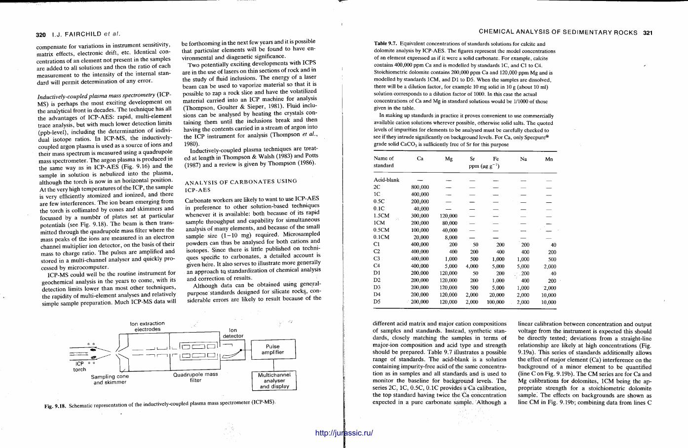
320 I.J. FAIRCHILD ef al.
compensa te for variations in instrument sensitivity, matrix effects, electronic drift, e tc . Identical concentrat ions of an e lement not present in the samples a re added to all solutions and then the ratio of each measurement to t he intensity of the internal standard will permit determinat ion of any error .
Inductively-coupled plasma mass spectrometry ( ICP-MS) is perhaps the most exciting development on the analytical front in decades . The technique has all the advantages of I C P - A E S : rapid, mult i-element trace analysis, but with much lower detect ion limits (ppb-level) , including the determinat ion of individual isotope rat ios. In ICP-MS, the inductively-coupled argon plasma is used as a source of ions and their mass spectrum is measured using a quadrupole mass spectrometer . T h e argon plasma is produced in the same way as in I C P - A E S (Fig. 9.16) and the sample in solution is nebulized into the plasma, al though the torch is now in an horizontal position. At the very high tempera tures of the I C P , the sample is very efficiently atomized and ionized, and there are few interferences. T h e ion b e a m emerging from the torch is collimated by cones and skimmers and focussed by a number of plates set at particular potentials (see Fig. 9.18). T h e beam is then transmitted through the quadrupole mass filter where the mass peaks of the ions are measured in an electron channel multiplier ion detec tor , on t he basis of their mass to charge rat io. T h e pulses are amplified and stored in a multi-channel analyser and quickly processed by microcomputer .
ICP-MS could well be the rout ine instrument for geochemical analysis in the years to come , with its detection limits lower than most o the r techniques , the rapidity of mult i -element analyses and relatively simple sample prepara t ion . Much ICP-MS da ta will
be forthcoming in the next few years and it is possible that particular e lements will be found to have environmental and diagenetic significance.
T w o potentially exciting developments with ICPS are in the use of lasers on thin sections of rock and in the study of fluid inclusions. The energy of a laser beam can be used to vaporize material so tha t it is possible to zap a rock slice and have t he volatilized material carried into an ICP machine for analysis (Thompson , Goul te r & Sieper, 1981). Fluid inclusions can be analysed by heat ing the crystals containing them until the inclusions break and then having the contents carried in a s t ream of argon into the ICP instrument for analysis (Thompson et al., 1980).
Inductively-coupled plasma techniques are treated at length in Thompson & Walsh (1983) and Potts (1987) and a review is given by Thompson (1986).
A N A L Y S I S O F C A R B O N A T E S U S I N G I C P - A E S
Carbonate workers are likely to want to use ICP-AES in preference to other solution-based techniques whenever it is available: both because of its rapid sample throughput and capability for s imultaneous analysis of many e lements , and because of the small sample size (1 — 10 mg) required. Microsampled powders can thus be analysed for both cations and isotopes. Since there is little published on techniques specific to carbonates , a detailed account is given here . It also serves to illustrate more generally an approach t o standardization of chemical analysis and correction of results.
Al though data can b e obta ined using general-purpose s tandards designed for silicate rocks,, considerable errors a re likely t o result because of t he
ICP torch
Ion extraction electrodes
Sampling cone and skimmer
I C Z H
• • I
Quadrupole mass filter
Ion detector
Pulse amplifier
Multichannel analyser
and display
Fig. 9.18. Schematic representation of the inductively-coupled plasma mass spectrometer (ICP-MS).
CHEMICAL ANALYSIS OF SEDIMENTARY ROCKS 321
Table 9.7. Equivalent concentrations of standards solutions for calcite and dolomite analysis by ICP-AES. The figures represent the model concentrations of an element expressed as if it were a solid carbonate. For example, calcite contains 400,000 ppm Ca and is modelled by standards 1C, and CI to C4. Stoichiometric dolomite contains 200,000 ppm Ca and 120,000 ppm Mg and is modelled by standards 1CM, and Dl to D5. When the samples are dissolved, there will be a dilution factor, for example 10 mg solid in 10 g (about 10 ml) solution corresponds to a dilution factor of 1000. In this case the actual concentrations of Ca and Mg in standard solutions would be 1/1000 of those given in the table.
In making up standards in practice it proves convenient to use commercially available cation solutions wherever possible, otherwise solid salts. The quoted levels of impurities for elements to be analysed must be carefully checked to see if they intrude significantly on background levels. For Ca, only Specpure® grade solid C a C 0 3 is sufficiently free of Sr for this purpose
Name of standard
Ca Mg Sr Fe ppm ( u g g - 1 )
Na Mn
Acid-blank _ 2C 800,000 — — — — — 1C 400,000 — — — — — 0.5C 200,000 — — — — — 0.1C 40,000 — — — — — 1.5CM 300,000 120,000 — — — — 1CM 200,000 80,000 — — — — 0.5CM 100,000 40,000 — — — — 0.1CM 20,000 8,000 — — — — CI 400,000 200 50 200 200 40 C2 400,000 400 200 400 400 200 C3 400,000 1,000 500 1,000 1,000 500 C4 400,000 5,000 4,000 5,000 5,000 2,000 Dl 200,000 120,000 50 200 . 2 0 0 40 D2 200,000 120,000 200 1,000 400 200 D3 200,000 120,000 500 5,000 1,000 2,000 D4 200,000 120,000 2,000 20,000 2,000 10,000 D5 200,000 120,000 2,000 100,000 2,000 10,000
different acid matrix and major cation compositions of samples and s tandards. Instead, synthetic standards , closely matching the samples in terms of major-ion composit ion and acid type and strength should be prepared . Table 9.7 illustrates a possible range of s tandards . T h e acid-blank is a solution containing impurity-free acid of the same concentration as in samples and all s tandards and is used to moni tor the baseline for background levels. T h e series 2C, 1C, 0.5C, 0.1C provides a Ca calibration, the top s tandard having twice the Ca concentration expected in a pure carbonate sample. Al though a
linear calibration between concentrat ion and output voltage from the instrument is expected this should be directly tested; deviations from a straight-line relationship are likely at high concentrations (Fig. 9.19a). This series of s tandards additionally allows the effect of major e lement (Ca) interference on the background of a minor e lement to be quantified (line C on Fig. 9.19b). The C M series are for Ca and Mg calibrations for dolomites , 1CM being the appropr ia te strength for a stoichiometric dolomite sample. T h e effects on backgrounds are shown as line C M in Fig. 9.19b; combining data from lines C
http://jurassic.ru/
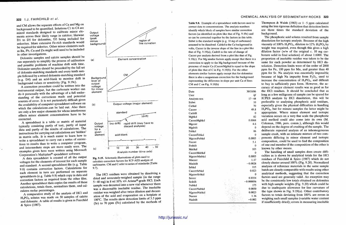
3 2 2 I.J. FAIRCHILD ef al.
and C M allows the separate effects of Ca and Mg on background to be quantified. Solutions C I to C4 a re mixed standards designed to calibrate minor elements across their likely range in calcites; likewise D l to D 5 for dolomites , D 5 being included for ankeri tes . More extensive Fe-rich s tandards would be required for siderites. O t h e r minor e lements such as Ba , Pb , Cu and Z n might well need to be included in other investigations.
Dolomite samples and calcite samples should b e run separately to simplify the process of calibration and possible problems of machine drift with t ime. Dolomi te samples should be preceded by the full set of dolomite-matching standards and every tenth sample followed by a mixed dolomite-matching s tandard (e .g. D4) and an acid-blank to monitor drift in background values or sensitivity (Fig. 9.19c).
A correction procedure could be written into the instrumental ou tput , but the carbonate worker can d o it personally with the advantage of a full understanding of the corrections m a d e and potential sources of er ror . It is not particularly difficult given the availability of compute r spreadsheet software on which the calculations >can be laid out . Also the re are only a few major elements for whose interference effects minor e lement concentrat ions have t o be corrected.
A spreadsheet is a table or matrix of material typically consisting part ly of text , part ly of input da ta and partly of the results of calculations. T h e instructions for carrying out calculations a re 'h idden ' in matrix cells. It is much easier t o learn how to write a spreadsheet to carry out a series of corrections to results than to write a computer p rogram, and in termediate steps are more easily seen. T h e examples given here were written using Microsoft Corporat ion 's Multiplan® speadsheet software.
A data spreadsheet is created of all the output voltages for the elements of interest for each sample and s tandard. A second spreadsheet file (e.g. Table 9.8) contains correction factors. Calculations for each element in turn are performed on separate spreadsheets (e.g. Table 9.9) which copy in da ta and correction factors as required from the other files. A n o t h e r spreadsheet then copies the results of these calculations, totals t h e m , normalizes t h e m , and calculates molar percentages .
A comparat ive study of the analysis of HC1 and H3PO4 solutes was made on 50 samples of calcite and dolomite . A table of results is given in Fairchild & Spiro (1987).
Output voltage (peak minus background)
(a)
Background level of output voltage for minor element
region of ine curvation
Element concentration
(b) Output voltage (major element)
Output voltage for a given element
standard (drift)
\ (no drift) rapid drift (may have to
discard analyses)
acid-blank
(c) 10 20 30 40 50
Analysis number (time axis)
Fig. 9.19. Schematic illustrations of plots used to calculate correction factors for ICP-AES analysis of carbonates. CM and C refer to series of standards (Table 9.7).
T h e HC1 residues were obtained by dissolving a dried and accurately-weighed sample (in the range 5 - 4 0 mg) in 8 ml 10% v/v Aristar®-grade HC1. Each sample was decanted into a new vial whenever there was a discernable insoluble res idue. T h e insoluble residue was weighed after twice dilution and decant-ation of the acid and evaporat ion on a hotplate at 100°C. The results show detection limits of 3.5 ppm (Sr) to 70 p p m (Fe) calculated by the me thods of
CHEMICAL ANALYSIS OF SEDIMENTARY ROCKS 323
Table 9.8. Example of a spreadsheet with factors used to correct data to concentrations. The analysis numbers identify which block of samples have similar correction factors (as identified on plots like that of Fig. 9.19c) and so can be corrected together by the factors in this table. Stdwt is the standard weight (e.g. 10 mg of carbonate) assumed to be dissolved. Cabkd is the Ca background in volts, Cacorr is the inverse slope of the line in a plot like that of Fig. 9.19(a), Cadrift is the rate of change of Cacorr per analysis derived from a plot like that of Fig. 9.19(c). For Mg similar factors apply except that there is a correction to apply to the Mg background because of the presence of major Ca (CacorrMgbkd is equal to the slope of plots like that of C in Fig. 9.19(b). For the other elements similar factors apply except that for dolomites there is also a magnesium correction for the background representing the difference in slope per unit Ca of lines CM and C o n Fig. 9.19(b)
Date 30/10/86 User ijf Analysis nos 17-44 Stdwt 10 Cabkd 70 Cacorr 49.8 Cadrift 0 Mgbkd 82 CacorrMgbkd 0.0068 Mgcorr 4.6 Mgdrift 0 Febkd 86 CacorrFebkd 0 MgcorrFebkd 0.0005 Fecorr 5.1 Fedrift 0 Mnbkd 103 CacorrMnbkd 0 MgcorrMnbkd 0.0005 Mncorr 1.17 Mndrift -0.0028 Srbkd 115 CacorrSrbkd 0.023 MgcorrSrbkd 0 Srcorr 0^0354 Srdrift -0.000056 Nabkd 175 CacorrNabkd 0.0050 MgcorrNabkd 0.0025 Nacorr • 1.36 Nadrift .. -0.002
Thompson & Walsh (1983) or 1 - 5 ppm calculated using the less rigorous definition that detection limits are three times the s tandard deviation of the background.
T h e phosphoric acid solutes resulted from sample dissolution for isotopic analysis. Because of the high viscosity of 100% H3PO4, dilution to 12% H 3 P 0 4 by weight was required, even though this gives a high dilution factor (w/w of the original c. 10 mg carbonate solid in final solution) of about 1:6000. The proport ion of insoluble residue was taken to be the same for each powder as determined by HC1 dissolution. Detect ion limits were of the order of 2000 ppm for F e , 100 ppm for M n , and greater than 40 ppm for Sr. Na analysis was essentially impossible because of high Na impurity from P2O5, used to increase the concentrat ion of H 3 P 0 4 , and difficult to buy in sufficiently pure form. However , the accuracy of major e lement results was as good as for the HC1 residues. It should be concluded that as long as a few milligrams of sample can be spared for I C P E S analysis by HC1 dissolution, this will be preferable to analysing phosphoric acid residues, especially given the physical difficulties in handling H 3 P 0 4 , but for minute samples the latter might be appropr ia te . Where minor e lement and isotopic variation occurs on a very fine scale the phosphoric acid method could also come into its own (M. Coleman, 1986, pers . comm. ) , al though this would depend on the degree of crushing of the sample. The deliberate repeated analysis of an inhomogeneous sample crush, with an intimate mixture of two components differing in minor element and isotopic composit ion, could be used to find the composition of one end member if the composit ion of the other is known by other means .
T h e handling of small samples does create difficulties as is shown by analytical totals for the HC1 residues of Fairchild & Spiro (1987) which do not closely cluster a round 100% (Fig. 9.20). Normalized analyses of reference materials in the same sample batch are closely comparable with results using other analytical me thods , suggesting that the correction factors used are generally valid. An exception may be the consistently low totals obtained on dolomites with high sample weights (Fig. 9.20) which could be due to inadequate allowance for line curvature of the type shown in Fig. 9.19(a). O the r contributory factors to totals deviating from 100% are errors in weighing such small samples (variable water content if insufficiently dr ied) ; errors in measuring insoluble
lllllUliU http://jurassic.ru/
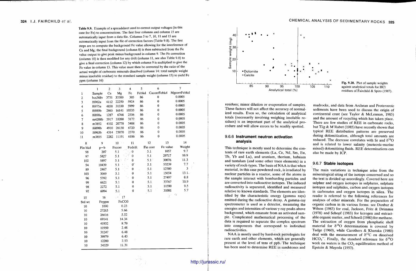
324 I.J. FAIRCHILD ef al. Table 9.9. Example of a spreadsheet used to correct output voltages (in this case for Fe) to concentrations. The first four columns and column 15 are automatically input from a data file. Columns 5 to 7, 10, 11 and 15 are automatically input from the file of correction factors (Table 9.8). The first steps are to compute the background Fe value allowing for the interference of Ca and Mg; the final background (column 8) is then subtracted from the Fe value output to give peak minus background in column 9. The Fe correction (column 10) is then modified for any drift (column 11, see also Table 9.8) to give a final correction (column 12) by which column 9 is multiplied to give the Fe value in column 13. This value must then be corrected by the ratio of the actual weight of carbonate minerals dissolved (column 14: total sample weight minus insoluble residue) to the standard sample weight (column 15) to yield Fe ppm (column 16)
1 2 3 4 5 6 7 1 Sample Ca Mg Fe Febkd CacorrFebkd MgcorrFebkd 2 bcs368v 3731 23300 305 86 0 0.0005 3 f6962a 4112 22250 5924 86 0 0.0005 4 f6975a 4858 31330 5999 86 0 0.0005 5 f6989b 2865 16141 10533 86 0 0.0005 6 f6890a 1287 6768 2556 86 0 0.0005
7 m4208b 5917 33200 3172 86 0 0.0005 8 m3852 4102 20770 5488 86 0 0.0005 9 f6890b 4910 26130 6720 86 0 0.0005
10 f6963b 4314 23070 2370 86 0 0.0005 11 m3855 2282 11191 6186 86 0 0.0005
8 9 10 11 12 13 14 Fin bkd p - b Fecorr Fedrift Fin corr Fe value Weight
98 207 5.1 0 5.1 1057 9.7 97 5827 5.1 0 5.1 29717 10.9
102 5897 5,1 0 5.1 30076 11.3 94 10439 5.1 0' 5.1 53239 7.7 89 2467 5.1 0 5.1 12580 3
103 3069 5.1 0 5.1 15654 13.1. 96 5392 5.1 0 5.1 27497 •8.8 99 6621 5.1 0 5.1 33767 10.9 98 2272 5.1 0 5.1 11590 9.5 92 6094 5.1 0 5.1 31081 5.7
15 16 . -: 17 Stdwt Feppm FeCC-3
10 1090 0.23 10 27263 5.66 10 26616 5.52 10 69141 14.34 10 41932 8.70 10 11950 2.48 10 31247 6.48 10 30979 6.43 10 12200 2.53 10 54529 11.31
CHEMICAL ANALYSIS OF SEDIMENTARY ROCKS
. . I »
• Dolomite x Calcite
85 90 95 100 Analytical total (%)
105 110 Fig. 9.20. Plot of sample weights against analytical totals for HC1 residues of Fairchild & Spiro (1987).
residues; minor dilution or evaporat ion of samples. These factors will not affect the accuracy of normalized results. Even so, the calculation of analytical totals (necessarily involving weighing insoluble residues) is an important part of the analytical procedure and will allow errors to be readily spotted.
9.6.6 Instrument neutron activation analysis
This technique is mostly used to de termine t he contents of rare earth e lements (La, Ce , Nd , Sm, E u , T b , Y b and Lu) , and uran ium, thor ium, hafnium and tan ta lum (and some o ther t race e lements) in a variety of rock-types. The basis of N A A is that when material , in this case powdered rock, is irradiated by nuclear particles in a reactor , some of the atoms in the sample interact with bombarding particles and are converted into radioactive isotopes. The induced radioactivity is separated, identified and measured relative to known s tandards . T h e elements are identified by the characteristic energy (gamma rays) emit ted during the radioactive decay. A gamma-ray spectrometer is used as a detector , measuring the energies and intensities of various y-ray peaks above background, which emana te from an activated sample . Complicated mathemat ical processing of the data is required to separate the complex spectrum into components that correspond to individual radioactivities.
N A A is mostly used by hard-rock penologis ts for rare ear th and other e lements , which are generally present at the level of tens of ppb.- The technique has been used to determine R E E in sands tones and
mudrocks , and data from Archean and Proterozoic sediments have been used t o discuss the origin of continental crust (see Taylor & McLennan , 1985) and the amount of recycling which has taken place. The re are few studies of R E E in carbonate rocks, but Tlig & M ' R a b e t (1985) have recently shown that typical R E E distribution pa t te rns are preserved during dolomitization, although total amounts are reduced. T h e decrease correlates with Sr and 8 l s O and is related to lower salinity (meteoric-marine mixed) dolomitizing fluids. R E E determinations can also be m a d e by ICP.
9.6.7 Stable isotopes
The main variations in technique arise from the mineralogical siting of the isotope concerned and so the text is divided up accordingly. Covered here are sulphur and oxygen isotopes in sulphates, sulphate isotopes and sulphides, ca rbon and oxygen isotopes in carbonates and oxygen isotopes in silica. The reader is referred to the following references for analyses of o ther minerals. For the preparat ion of organic carbon in its various forms: see Dunba r & Wilson (1983) for coal, Jackson, Fritz & Dr immie (1978) and Schopf (1983) for kerogen and extract-able organic mat ter , and Schoell (1980) for methane . T h e extraction of oxygen from phosphat ic shell material for 5 l s O determinat ions is covered by Tudge (1960), while Carothers & Kharaka (1980) deal with the measurement of 5 1 3 C on dissolved H C 0 3 ~ ! Finally, the s tandard reference for 5 l s O work on waters is the C 0 2 equilibration method of Epstein & Mayeda (1953).
http://jurassic.ru/
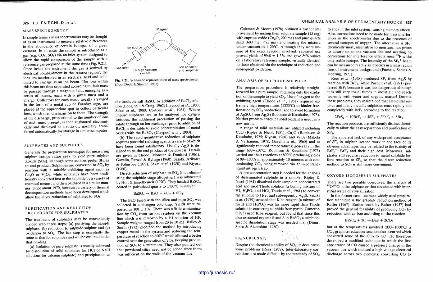
326 I.J. FAIRCHILD ET AL.
MASS S P E C T R O M E T R Y
In simple terms a mass spect rometer may be thought of as an instrument to measure relative differences in the abundance of certain isotopes of a given e lement . In all cases the sample is introduced as a gas (e.g. C 0 2 , S O 2 ) via an inlet system designed to allow the rapid comparison of the sample with a reference gas prepared at the same time (Fig. 9.21). Once inside the instrument the gas is ionized by electrical bombardmen t in the 'source region ' , the ions are accelerated in an electrical field and colli-mated to emerge as an ion beam. The ions within this beam are then separated according to their mass by passage through a magnetic field, emerging as a series of beams, each with a given mass and a charge. Collectors for each mass, usually ar ranged in the form of a metal cup or Faraday cage, are placed at the appropr ia te spot to collect particular ions, which then discharge on to them. T h e strength of the discharge, proport ional to the number of ions of each mass present , is then registered electronically and displayed as a ratio or, normally, transferred automatically for s torage in a microcomputer .
S U L P H A T E S A N D S U L P H I D E S
General ly the prepara t ion techniques for measuring sulphur isotope ratios seek to yield pure sulphur dioxide ( S 0 2 ) , al though some authors prefer S F 6 as an end-product . Sulphides a re converted t o S 0 2 by reaction with a suitable oxidizing agent such as C u 2 0 or V 2 0 5 , while sulphates have been traditionally converted first to the sulphide by a variety of chemical means , and then oxidized in a similar manner. Since about 1970, however , a variety of thermal decomposit ion methods have been developed which allow the direct reduction of sulphates to S 0 2 .
P U R I F I C A T I O N A N D R E D U C T I O N P R O C E D U R E S F O R S U L P H A T E S
The t rea tment of sulphates may be conveniently divided into three steps: (a) purifying the sample sulphate , (b) reduct ion to sulphide-sulphur and (c) oxidation to S O z . The last s tep is essentially the same as that for sulphides and will be outlined under that heading.
(a) Isolation of pure sulphate is usually achieved by dissolution of solid sulphates (in HC1 or NaCl solutions for calcium sulphate) and precipitation as
Magnet
To high-vacuum a n c j amplifier system
Fig. 9.21. Schematic representation of mass spectrometer (from Dodd &,Stanton, 1981).
the insoluble salt B a S 0 4 by addition of B a C l 2 solution (Longinelli & Craig, 1967; Claypool etal., 1980; Sakai et al., 1980; Cortecci et al., 1981). W h e r e impure sulphates are t o b e analysed for oxygen isotopes, the additional precaution of passing the solute through an ion-exchanger prior to addit ion of B a C l 2 is desirable to avoid coprecipitation of metal oxides with the B a S 0 4 (Claypool et al., 1980).
(b) The rapid quanti tat ive reduct ion of sulphate requires powerful reducing agents , a variety of which have been found satisfactory. Usually A g 2 S is designed to be the end-product of the process. Details are given in T h o d e , Monster & Dunford (1961), Gavel in , Parwel & Ryhage (1960), Sasaki , Ar ikawa & Folinsbee (1979), Sakai et al. (1980) and Kiyosu (1980).
Direct-reduction of sulphate t o S 0 2 ( thus eliminating the sulphide stage al together) was advocated by Hol t & Engelkemeir (1970). They headed B a S 0 4
coated in pulverized quar tz to 1400°C in vacuo:
B a S 0 4 -»• B a O + ?02 + S O z .
The B a O fused with the silica and pure S 0 2 was collected in a nitrogen cold t rap . Yields were repor ted as 100 ± 1 % . T h e r e was a little contamination by C 0 2 from carbon residues on the vacuum line which was removed by a 1:1 solution of H F . Sample weights ranged from 20 to 50 mg. Bailey & Smith (1972) modified the method by introducing copper metal to the system and reducing the tempera ture of reaction to 800°C which allowed a bet ter control over the generat ion of S 0 2 , keeping production of SO3 to a minimum. They also pointed out that powdered silica need not be added since there was sufficient on the walls of the vacuum line.
CHEMICAL ANALYSIS OF SEDIMENTARY ROCKS 327
Coleman & Moore (1978) outlined a further improvement by mixing their sulphate sample (15 mg) with cuprous oxide ( C u 2 0 , 200 mg) and pure quar tz sand (600 mg, < 7 5 um) and heating the mixture under vacuum to 1120°C. Al though they were unsure of the exact reaction involved, repeated use proved yields of 99.8 ± 1.3% and gave 5 3 4 S values on a laboratory reference sample , virtually identical to those obtained via the technique of reduction and subsequent oxidation.
A N A L Y S I S O F S U L P H I D E - S U L P H U R
The preparat ion procedure is relatively straightforward for a pure sample , requiring only the oxidation of the sample to yield S 0 2 . Use of oxygen as the oxidizing agent (Thode et al., 1961) required extremely high tempera tures (1350°C) to hinder fractionation by S 0 3 product ion, and to avoid formation of A g S 0 4 from A g 2 S (Robinson & Kusakabe , 1975). Nei ther problem arises if a solid oxidant is used, as is now normal .
A range of solid materials are utilized including C u O (Ripley & Nicol, 1981), C u 2 0 (Robinson & Kusakabe , 1975; Kiyosu, 1980) and V 2 0 5 (Makela & Vart ia inen, 1978; Gavel in et al., 1960) and at significantly reduced tempera tures ; generally in the range 600-850°C. Robinson & Kusakabe (1975) carried out their reactions at 800°C producing yields of 99—100% in approximately 10 minutes with contaminating C 0 2 being removed via an «-pentane-liquid nitrogen t rap .
A pre-concentration step is needed for the analysis of disseminated sulphide in a sample. Ripley & Nicol (1981) dissolved their sample in concentrated acid and used Thode solution (a boiling mixture of H I , H 3 P 0 4 and HC1, Thode et al., 1961) to convert the sulphur to H 2 S , and subsequently A g 2 S . Sasaki et al. (1979) stressed that Kiba reagent (a mixture of tin I I and H3PO4) was far more rapid than T h o d e solution in extracting sulphide from pyrite. Cameron (1983) used Kiba reagent , but found that since this also extracted organic S and S in B a S 0 4 a sulphide-specific dissolution stage was needed first (Dinur , Spiro & Aizenshtat , 1980).
S 0 2 V E R S U S SI„
Despi te the chemical stability of S O , , it does cause some problems (Rees , 1978). INTER-laboratory correlations are made difficult by the tendency of S 0 2
to stick in the inlet system, causing memory effects. Also , corrections need to be m a d e for mass interferences in the spectrometer due to the presence of several isotopes of oxygen. The alternative is S F 6 : chemically inert , insensitive to moisture , not p rone to adsorb on to the vacuum line and needing no corrections for interference effects since 1 9 F is the only stable isotope. The intensity of the S F 5
+ beam can be measured readily as it occurs in a mass region free of instrument background (Puchelt , Sables & Hoer ing , 1971).
Rees et al. (1978) produced S F 6 from A g 2 S by reaction with B r F 5 , while Puchelt et al. (1971) preferred B r F 3 because it was less dangerous; al though it is still very toxic, fumes in moist air and reacts violently with water and organic matter! Despi te these problems, they maintained that elemental sulphur and many metallic sulphides react rapidly and completely with B r F 3 according to the reaction:
2 F e S 2 + 10BrF 3 4 S F 6 + 2 F e F 3 + 5Br 2 .
The reaction products are sufficiently distinct chemically to allow the easy separation and purification of S F 6 .
The apparent lack of any widespread acceptance of SF6 in sulphur isotope work in the face of its obvious advantages may be related to the toxicity of B r F 5 ~ —BrF 3 and their high cost. Moreover , sulphates still require reduction to metal sulphide before reaction to S F 6 so that the direct reduction method to S 0 2 is still more convenient.
O X Y G E N I S O T O P E S IN S U L P H A T E S
There are two possible objectives: the analysis of 1 8 0 / 1 6 0 in the sulphate or that associated with interstitial water of crystallization.
In the former case, the most widely used preparation technique is the graphite reduction method of Rafter (1967). Earl ier work by Rafter (1957) had proved the general feasibility of producing C 0 2 by reduction with carbon according to the reaction:
B a S 0 4 + 2 C ^ BaS + 2 C 0 2
but at the tempera tures involved (900-1000°C) a C 0 2 - g r a p h i t e reduction reaction also occurred which converted some of the C 0 2 to C O . H e therefore developed a modified technique in which the first appearance of C O caused a pressure change in the vacuum line which induced a high voltage electrical discharge across two elements; converting C O to
http://jurassic.ru/
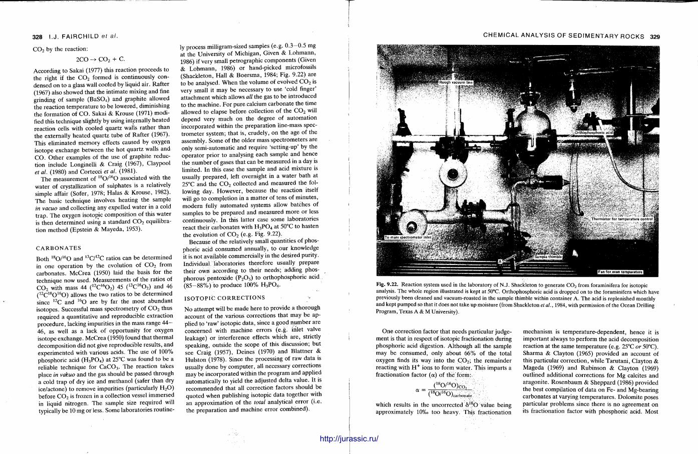
328 I.J. FAIRCHILD ef al.
C O z by the reaction:
2 C O -> C 0 2 + C.
According to Sakai (1977) this reaction proceeds to the right if the C 0 2 formed is continuously condensed on to a glass wall cooled by liquid air. Rafter (1967) also showed that the int imate mixing and fine grinding of sample ( B a S 0 4 ) and graphite allowed the reaction t empera tu re t o be lowered, diminishing the formation of C O . Sakai & Krouse (1971) modified this technique slightly by using internally hea ted reaction cells with cooled quartz walls ra ther than the externally heated quar tz tube of Rafter (1967). This eliminated memory effects caused by oxygen isotope exchange between the hot quar tz walls and C O . O the r examples of the use of graphite reduction include Longinelli & Craig (1967), Claypool et al. (1980) and Cortecci et al. (1981).
T h e measurement of 1 8 0 / 1 6 0 associated with the water of crystallization of sulphates is a relatively simple affair (Sofer, 1978; Halas & Krouse , 1982). T h e basic technique involves heat ing the sample in vacuo and collecting any expelled water in a cold t rap . T h e oxygen isotopic composit ion of this water is then determined using a standard C 0 2 equilibration method (Epstein & Mayeda , 1953).
C A R B O N A T E S
Both 1 8 0 / 1 6 0 and 1 3 C / 1 2 C ratios can be de termined in one operat ion by the evolution of C 0 2 from carbonates . McCrea (1950) laid the basis for the technique now used. Measurements of the ratios of C 0 2 with mass 44 ( 1 2 C 1 6 0 2 ) 45 ( 1 3 C 1 6 0 2 ) and 46 ( 1 2 C 1 8 0 1 6 0 ) allows the two ratios to be de te rmined since 1 2 C and 1 6 0 are by far the most abundant isotopes. Successful mass spectrometry of C 0 2 thus required a quanti tat ive and reproducible extraction procedure , lacking impurities in the mass range 44— 46, as well as a lack of opportunity for oxygen isotope exchange. McCrea (1950) found that thermal decomposit ion did not give reproducible results, and exper imented with various acids. The use of 100% phosphoric acid ( H 3 P 0 4 ) at 25°C was found to be a reliable technique for C a C 0 3 . The reaction takes place in vakuo and the gas should be passed through a cold t rap of dry ice and methanol (safer than dry ice/actone) to remove impurities (particularly H 2 0 ) before C 0 2 is frozen in a collection vessel immersed in liquid nitrogen. The sample size required will typically be 10 mg or less. Some laboratories rout ine
ly process milligram-sized samples (e.g. 0.3—0.5 mg at the University of Michigan, Given & L o h m a n n , 1986) if very small petrographic components (Given & L o h m a n n , 1986) or hand-picked microfossils (Shackleton, Hall & Boersma, 1984; Fig. 9.22) are to be analysed. W h e n the volume of evolved C 0 2 is very small it may be necessary t o use 'cold finger' a t tachment which allows all the gas to be introduced to the machine. For pure calcium carbonate the t ime allowed to elapse before collection of the C 0 2 will depend very much on the degree of automat ion incorporated within the preparat ion line-mass spect rometer system; that is , crudely, on the age of the assembly. Some of the older mass spectrometers are only semi-automatic and require ' set t ing-up' by the operator prior to analysing each sample and hence the number of gases that can be measured in a day is limited. In this case the sample and acid mixture is usually p repa red , left overnight in a water bath at 25°C and the C 0 2 collected and measured the following day. However , because the react ion itself will go to completion in a mat ter of tens of minutes , modern fully au tomated systems allow batches of samples to be p repared and measured more o r less continuously. In this latter case some laboratories react their carbonates with H 3 P 0 4 at 50°C to hasten the evolution of C 0 2 (e.g. Fig. 9.22).
Because of the relatively small quantit ies of phosphoric acid consumed annually, to our knowledge it is no t available commercially in the desired puri ty. Individual laboratories therefore usually p repare their own according to their needs ; adding phosphorous pentoxide ( P 2 O s ) to or thophosphor ic acid ( 8 5 - 8 8 % ) to produce 100% H 3 P 0 4 .
I S O T O P I C C O R R E C T I O N S
N o a t tempt will be made here to provide a thorough account of the various corrections that may be applied to ' r aw ' isotopic da ta , since a good number are concerned with machine errors (e.g. inlet valve leakage) or interference effects which are , strictly speaking, outside the scope of this discussion; but see Craig (1957), Deines (1970) and Blat tner & Hulston (1978). Since the processing of raw data is usually done by computer , all necessary corrections may be incorporated within the program and applied automatically to yield the adjusted delta value. It is recommended that all correction factors should be quoted when publishing isotopic data together with an approximation of the total analytical error (i .e. the prepara t ion and machine er ror combined) .
CHEMICAL ANALYSIS OF SEDIMENTARY ROCKS 329
Fig. 9.22. Reaction system used in the laboratory of N.J. Shackleton to generate C 0 2 from foraminifera for isotopic analysis. The whole region illustrated is kept at 50°C. Orthophosphoric acid is dropped on to the foraminifera which have previously been cleaned and vacuum-roasted in the sample thimble within container A. The acid is replenished monthly and kept pumped so that it does not take up moisture (from Shackleton et al., 1984, with permission of the Ocean Drilling Program, Texas A & M University).
O n e correction factor that needs particular judgement is that in respect of isotopic fractionation during phosphoric acid digestion. Al though all the sample may b e consumed, only about 6 6 % of t he total oxygen finds its way into the C 0 2 ; the remainder reacting with H + ions to form water . This imparts a fractionation factor ( a ) of the form;.
( l K 0/ ' 6 0)co . a ~ r l 8 n/ l 6 rv>
v '-Vcarbonale. which results in the uncorrected 6 1 8 b value being approximately 10% o too heavy. This fractionation
mechanism is t empera ture -dependent , hence it is important always to perform the acid decomposit ion reaction at the same temperature (e.g. 25°C or 50°C). Sharma & Clayton (1965) provided an account of this particular correction, while Taru tan i , Clayton & Mageda (1969) and Rubinson & Clayton (1969) outlined additional corrections for Mg calcites and aragoni te . Rosenbaum & Sheppard (1986) provided the best compilation of data on Fe- and Mg-bearing carbonates at varying tempera tures . Dolomi te poses particular problems since there is no agreement on its fractionation factor with phosphoric acid. Most
liiiiimiimiiiiiiifliiiiif http://jurassic.ru/
330 I.J. FAIRCHILD et al.
authors after 1965 followed Sharma & Clayton (1965) in applying a correction that approximates to — 0.8%o with respect to calcite. Land (1980) noted that corrections applied were varied, and often no t s ta ted. Both he and Rosenbaum & Sheppard (1986) found a substantially larger correction most likely in the light of their experimental evidence, although Land (1980) recommended treating all carbonates effectively as calcites in this respect until the mat te r is resolved. Clearly it is very important to state the phosphoric acid correction factor used in published repor ts .
P R E P A R A T I O N O F C A R B O N A T E S O T H E R T H A N C a C 0 3 A N D M I X E D C A R B O N A T E S A M P L E S
The standard prepara t ion method of McCrea (1950) outlined above was designed specifically t o cope with calcium carbonate , either as calcite or aragonite which react readily with phosphoric acid at room tempera ture . With other carbonate species, however, the reaction at 25°C is very much slower and can considerably lengthen the t ime to process each sample. Becker & Clayton (1972) prepared samples of calcite, dolomite , ankeri te and siderite at 25°C and found that while the calcite reaction was complete in 24 hours , periods of one week , two weeks and two to three months respectively were required for the remainder . No t only a re such extended periods of reaction inconvenient in rout ine work but there is always a danger that the reaction vessel may leak while not being actively p u m p e d , leading to contaminat ion with atmospheric C 0 2 . F ine grinding of t he sample t o increase the total surface a rea can be used to speed u p the reaction but such t rea tment is t ime-consuming and may cause isotopic exchange with the a tmosphere . Much more convenient is t o increase the reaction t empera tu re . Gould & Smith (1979), for example , working with siderite, initially mixed sample and acid at 80°C and then allowed the mixture to react at 25°C for 72 hours . Standard calcites t reated in the same manner showed no change in 5 1 3 C although 5 1 8 0 values were found to be too light by 1.2%o and hence all oxygens were corrected by this amount (see also Gaut ie r , 1982). Raising the reaction t empera tu re is particularly useful when working with dolomites , which at 50°C react to complet ion overnight. Bear ing in mind the temperature-related changes in the phosphoric acid correction factor, the s tandards should be run at the same tempera ture .
Mixtures of carbonates , particularly calcite and dolomite , often need to be analysed. If the composition of only one of the minerals is needed , it may be possible to remove it physically (see microsampling section), otherwise a chemical pre- t rea tment is required. Videtich (1981) ground the sample to < 3 um and selectively leached the calcite with E D T A (Glover , 1961) in order to analyse the dolomite , but warned that this method was not suitable for calcian dolomites which dissolve more readily in E D T A . Wada & Suzuki (1983), seeking to analyse calcite in dolomitic marbles , ground samples to <50- um and used a heavy-liquid method to separate the calcite. O t h e r techniques include that of Magari tz & Kafri (1981) who removed calcite by dissolution in 3 % HC1 and Land (1973) who used a dilute acetic acid digestion, bo th sets of authors using X R D techniques to prove the purity of the remaining dolomite . When it is necessary to know the isotopic composition of both minerals present, and physical separation is not possible, chemical methods are again necessary. T h e most favoured method of separat ion (although not without its critics) makes use of the variable reaction rates of calcite and dolomite with phosphoric acid; a technique originally p ioneered by Epste in , Graf & Degens (1964) and Degens & Epste in (1964). In their exper iments , mixtures of calcite and dolomite having first been ground to < 5 0 pm were reacted with phosphoric acid at 25°C and the C d 2 p roduced in the first hour (assumed to be principally from the more reactive calcite phase) analysed on the mass spectrometer . T h e reaction was then allowed to proceed for a further three ' hours during which t ime the C 0 2 formed was pumped away, while the remainder of t he gas produced from the fourth hour u p to a maximum of 72 .hours was assumed to represent the dolomitic fraction. H e n c e , they believed that by using this double collection procedure it was possible to de termine the isotopic composit ion of both minerals with minimal cross contaminat ion; a l though they suggested it was unsuitable for samples in which the two phases differed greatly in isotopic composit ion or where the ratio of one mineral to the other was large. M o r e recently Wal ters , Claypool & Choque t t e (1972) have pointed out tha t unless close bracketing of grain size is a t tempted by sieving, the large range of grain sizes will introduce errors into this technique because of the variable solubility in H 3 P 0 4 . Despi te these problems many workers have made use of the double collection procedure and a number of modifica-
CHEMICAL ANALYSIS OF SEDIMENTARY ROCKS 331
tions have been made to meet specific needs. Clayton et al. (1968) altered their reaction times to cope with very fine-grained samples while Becker & Clayton (1972) used the method to separate ankeri te and siderite.
R E M O V A L O F O R G A N I C M A T T E R
The presence of organic carbon in samples of carbonate leads to the introduction of volatile substances into the mass spectrometer which form a variety of reaction products in the ionization chamber and interfere with the weak mass 45 and 46 ion beams.
Al though pre- t rea tments for the removal of organic mat ter are most relevant to Recent skeletal aragonite , which has a very high organic content , it repays to give some thought to the effect on ancient carbonates . Charef & Sheppard (1984) no ted that sulphur-rich organic material is particularly t roublesome.
By far the simplest technique for removing organic carbon involves soaking the sample in a solution of sodium hypochlorite ( N a C 1 0 3 , clorox) or hydrogen peroxide ( H 2 0 2 ) to oxidize the organic material (e.g. Wefer & Berger , 1981; Cummings & McCarty , 1982). A more e laborate procedure was developed by Epstein et al. (1953) and involved ' roasting' the sample in a continuous stream of helium which swept away the decomposit ion products of the heated organic materials and preserved the sample in an iner t a tmosphere . W e b e r et al. (1976), Land , Long & Barnes (1977), Durazzi (1977) and Weil et al. (1981) a re among those tha t have a t tempted experimental work to quantify the effectiveness of each of these techniques and any isotopic fractionation effects they may have. The general consensus is that nei ther the c l o r o x / H 2 0 2 t rea tments nor high tempera ture roasting are capable of removing all organic carbon and there is considerable evidence that the former will impart some error to the measured isotopic value; a l though provided all samples are p repared in the same manner any errors will be systematic. Because of the possibility of some organic carbon remaining even after thorough pre-t rea tment , Weber et al. (1976) devised a rejection procedure based on a careful examination of the reference and sample chart recorder traces that al lowed an excessive input from organic mat ter t o be recognized. It should also be noted that roasting is
not suited to aragonite samples since some conversion of the unstable phase to calcite is likely under the high tempera ture conditions.
M I C R O S A M P L I N G
In common with chemical analyses discussed elsewhere , the effectiveness of isotope studies on carbonates is often greatly enhanced by being able to resolve differences be tween individual rock components such as grain and cement types (Hudson , 1977a).
O n e of the most popular methods of microsampling carbonate rocks is t o use a dental drill modified to accept very small drill bits which ideally need to be < 0 . 5 mm in diameter . Prezbindowski (1980) outlined some of the requirements of such a sampling procedure and described a miniature vertical milling machine developed for such a role and capable of both vertical and horizontal (furrow) cutting movements .
A precise, but more t ime-consuming alternative is to use a scalpel or razor blade to cut out particular components of interest from a thin-section. Dickson & Coleman (1980) used mult iple 40 pm thin sections cut from a single hand specimen which had been m o u n t e d in Lakes ide 70 and stained. Samples of > 5 mg were cut from each thin section using a scalpel and binocular microscope and they were able to prove that nei ther the mount ing glue nor the stain affected the measured isotopic composition of the carbonate .
S I L I C A T E S
Techniques designed for crystalline rocks have been adapted for sedimentary silicates. 1 8 0 / 1 6 0 and D / H ratios are the only important ones; see Douthi t t (1982) for silicon isotopes.
O X Y G E N IN S I L I C A T E S
Oxygen isotope rat io measurements are performed exclusively on C 0 2 in preference to 0 2 because it lies in a mass region relatively free of background interference. Moreover , C 0 2 is less reactive than 0 2
and thus less likely to be involved in chemical reactions with substances within the preparat ion line-mass spectrometer assembly which could introduce an isotope fractionation effect. Hence , the method
http://jurassic.ru/
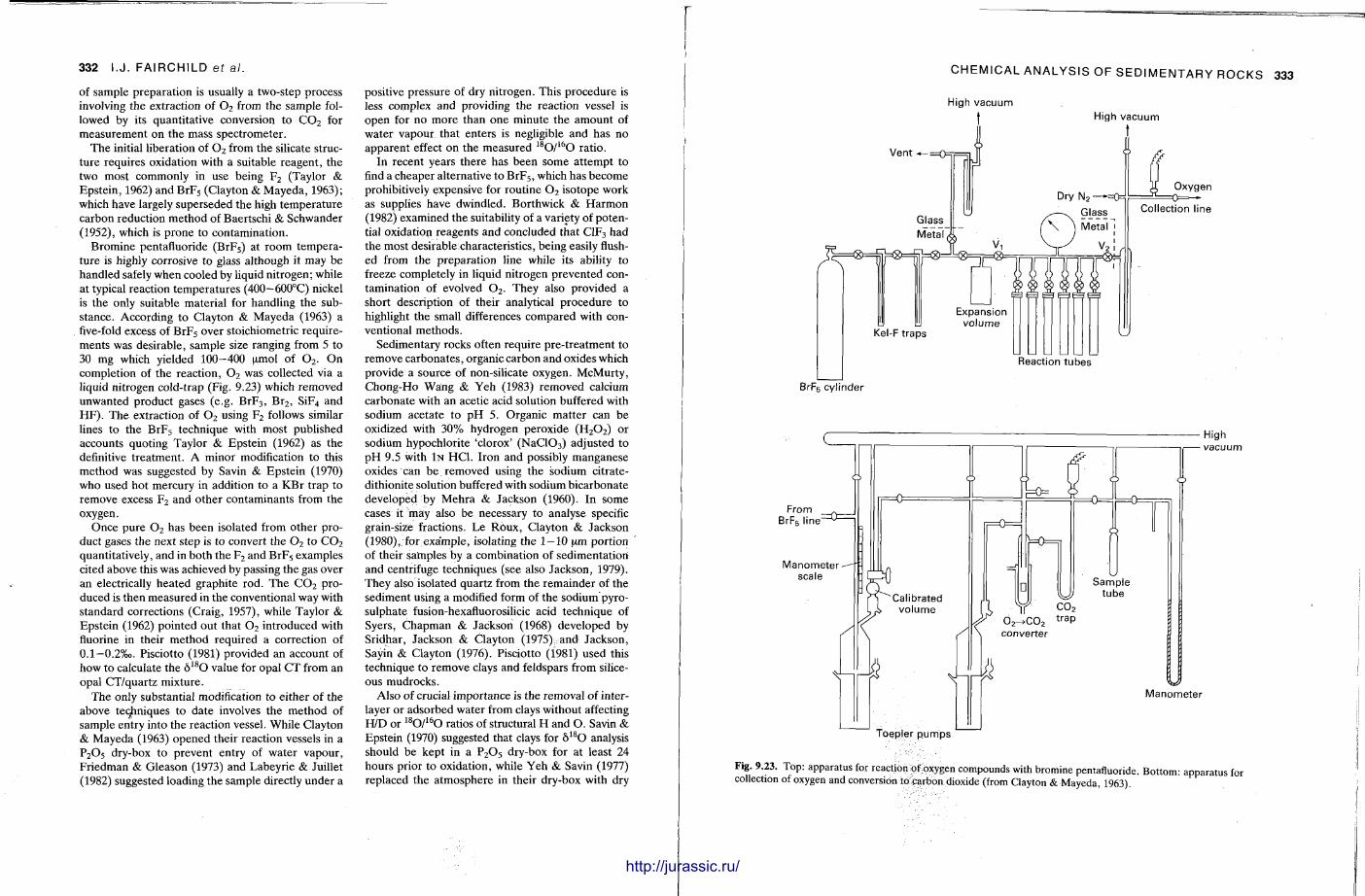
332 I.J. FAIRCHILD ef a l .
of sample preparat ion is usually a two-step process involving the extraction of 0 2 from the sample followed by its quanti tat ive conversion to C 0 2 for measurement on the mass spectrometer .
The initial liberation of 0 2 from the silicate structure requires oxidation with a suitable reagent , the two most commonly in use being F 2 (Taylor & Epste in , 1962) and B r F 5 (Clayton & Mayeda , 1963); which have largely superseded the high tempera ture carbon reduction method of Baertschi & Schwander (1952), which is prone to contaminat ion.
Bromine pentafluoride (BrF 5 ) at room temperature is highly corrosive to glass al though it may be handled safely when cooled by liquid ni trogen; while at typical reaction tempera tures (400—600°C) nickel is the only suitable material for handling the substance. According to Clayton & Mayeda (1963) a five-fold excess of B r F 5 over stoichiometric requirements was desirable, sample size ranging from 5 to 30 mg which yielded 1 0 0 - 4 0 0 pmol of 0 2 . O n completion of the reaction, 0 2 was collected via a liquid nitrogen cold-trap (Fig. 9.23) which removed unwanted product gases (e.g. B r F 3 , B r 2 , S iF 4 and H F ) . T h e extraction of 0 2 using F 2 follows similar lines to the B r F 5 technique with most published accounts quoting Taylor & Epstein (1962) as the definitive t rea tment . A minor modification to this method was suggested by Savin & Epstein (1970) who used hot mercury in addition to a KBr t rap to remove excess F 2 and other contaminants from the oxygen.
Once pure 0 2 has been isolated from other product gases the next s tep is to convert the 0 2 to C 0 2
quantitatively, and in both the F 2 and B r F 5 examples cited above this was achieved by passing the gas over an electrically heated graphite rod. The C 0 2 p roduced is then measured in the conventional way with standard corrections (Craig, 1957), while Taylor & Epstein (1962) pointed out that 0 2 introduced with fluorine in their method required a correction of 0.1—0.2%o. Pisciotto (1981) provided an account of how to calculate the 5 l s O value for opal C T from an opal CT/quartz mixture .
The only substantial modification to ei ther of the above techniques to date involves the me thod of sample entry into the reaction vessel. While Clayton & Mayeda (1963) opened their reaction vessels in a P 2 0 5 dry-box to prevent entry of water vapour , Fr iedman & Gleason (1973) and Labeyrie & Juillet (1982) suggested loading the sample directly under a
positive pressure of dry ni t rogen. This procedure is less complex and providing the reaction vessel is open for no more than one minute the amount of water vapour that enters is negligible and has no apparent effect on the measured 1 8 0 / 1 6 0 rat io.
In recent years there has been some a t tempt to find a cheaper alternative to B r F 5 , which has become prohibitively expensive for rout ine 0 2 isotope work as supplies have dwindled. Borthwick & H a r m o n (1982) examined the suitability of a variety of potential oxidation reagents and concluded that C1F 3 had the most desirablecharacter is t ics , being easily flushed from the preparat ion line while its ability to freeze completely in liquid nitrogen prevented contamination of evolved 0 2 . They also provided a short description of their analytical procedure to highlight the small differences compared with conventional methods .
Sedimentary rocks often require pre- t rea tment to remove carbonates , organic carbon and oxides which provide a source of non-silicate oxygen. McMurty , Chong-Ho Wang & Yeh (1983) removed calcium carbonate with an acetic acid solution buffered with sodium acetate to p H 5. Organic mat ter can be oxidized with 3 0 % hydrogen peroxide ( H 2 0 2 ) or sodium hypochlorite 'clorox' ( N a C 1 0 3 ) adjusted to p H 9.5 with I N HC1. I ron and possibly manganese oxides can be removed using the sodium citrate-dithionite solution buffered with sodium bicarbonate developed by Mehra & Jackson (1960). In some cases it may also be necessary to analyse specific grain-size fractions. Le Roux , Clayton & Jackson (1980), for example , isolating the 1 — 10 urn port ion of their samples by a combination of sedimentat ion and centrifuge techniques (see also Jackson, 1979). They also isolated quartz from the remainder of the sediment using a modified form of the sodium pyro-sulphate fusion-hexafluorosilicic acid technique of Syers, Chapman & Jackson (1968) developed by Sridhar, Jackson & Clayton (1975) ;and Jackson, Sayin & Clayton (1976). Pisciotto (1981) used this technique to remove clays and feldspars from siliceous mudrocks .
Also of crucial importance is the removal of inter-layer or adsorbed water from clays without affecting H/D or 1 8 0 / 1 6 0 ratios of structural H and O . Savin & Epstein (1970) suggested that clays for 5 1 8 0 analysis should be kept in a P 2 0 5 dry-box for at least 24 hours prior to oxidation, while Yeh & Savin (1977) replaced the a tmosphere in their dry-box with dry
CHEMICAL ANALYSIS OF SEDIMENTARY ROCKS
High vacuum
t High vacuum
Reaction tubes
BrF5 cylinder
From BrF6 line
Manometer scale
Calibrated volume
Toepler pumps
\ C O
2 ^ C 0 2
t r a P converter
ft
Sample tube
High • vacuum
v*4>
Manometer
Fig. 9.23. Top: apparatus for reaction pfoxygen compounds with bromine pentafluoride. Bottom: apparatus for collection of oxygen and conversion to carbon dioxide (from Clayton & Mayeda, 1963).
http://jurassic.ru/
334 I.J. FAIRCHILD ef al.
nitrogen two hours after the sample had been introduced. The small amount of water vapour remaining after 24 hours was not expected to effect the measured 6 1 8 0 value by more than a few tenths per mil. Particular care should be taken when prepar ing smectitic clays which have the ability to adsorb relatively large amounts of water and may require more thorough drying.
For H / D measurements preliminary out-gassing needs to be much more intensive. Savin & Epstein (1970) recommended heating the sample under vacuum at 100-250°C for 24 hours or more , while Y e h (1980) dried his samples at between 250 and 300°C for not less that three hours followed by storage in a nitrogen filled P2O5 dry-box. Both methods should be capable of removing virtually all adsorbed and inter-layer water .
D / H R A T I O M E A S U R E M E N T S ON S I L I C A T E S
The measurement is performed on hydrogen gas which is prepared by a fairly s tandard technique. The initial step after out-gassing is to extract hydrogen from the silicate structure as molecular water by heat ing the sample under vacuum at high temperatu re , anywhere between 900°C (Savin & Epste in , 1970) and 1500-1700°C (Godfrey, 1962). Since some hydrogen is also liberated in the molecular form this is converted to water by reaction with C u O . This water may then be quantitatively converted to H 2 by reaction with hot uranium (400—700°C) or ho t zinc after which it is collected via a liquid nitrogen cold t rap (Bigeleisen, Perlman & Prosser, 1952; Craig, 1961a, b ; Godfrey, 1962; Coleman etal., 1983). The evolved H 2 is measured isotopically against a suitable reference with a correction being m a d e for the H 3 + ion interference effect (Fr iedman, 1953). Because of the frequently large deviation from the s tandard, 6 D values may be quoted in per cent ra ther than parts per mil when necessary.
9.7 A N A L Y T I C A L Q U A L I T Y
9.7.1 Accuracy and precision
When chemical concentrat ions have been obtained it is desirable to know both their internal consistency and their relation to the ' t rue ' concentrat ion.
If a single technique is used to analyse repeatedly a perfectly homogeneous geological material then a range of results will be obtained for the elemental concentrat ion(s) . The variation arises because of the small errors introduced at all stages of the preparation and measurement of the sample , and if sufficient replicates are plot ted as a frequency diagram they will generally follow a Gaussian distribution. The results can thus be described by the mean (x) and the s tandard deviation (s), the latter te rm being known as the repeatabili ty (reproducibility is often used synonymously but it may also be used for the specific meaning of the variation between laboratories which have analysed that sample by the same method) . Relative repeatability is more convenient than s tandard deviation with the terms relative standard deviation (rsd = six), coefficient of variation (C = s /x .100%) and precision ( P = 2s/*. 100%) being used. Precision is often used loosely instead of repeatabili ty.
Accuracy is the extent to which the mean approaches the ' t rue ' concentrat ion and bias the difference between the mean or median and the ' t rue ' value. For geological materials the t rue concentration is unknowable and is approximated by a consensus 'usable value ' (see Section 9.7.2).
T h e propert ies of the Normal distribution allow an analyst to predict the propor t ion of the total number of measurements which lie be tween the given ranges (for a Gaussian distribution 6 8 . 3 % of observations lie in the range x ± s). This allows criteria for the rejection of results which may be in error , the rejection limit usually being set at 9 5 % confidence (strictly this is ±1 .96s but is usually approximated to ±2s). It should be stressed that 5 % of valid results will b e rejected and possibly some erroneous results accepted. T h e observations in error are usually te rmed 'fliers' and arise from unusual situations, for example the misreading of a balance or transient electrical 'noise ' . They can usually b e detected where there are a large number of replicates but when , for example , only triplicate measurements are available the rejection limits in terms of j become very large (x ± 10s) (Harvey, 1974). W h e r e fliers are present the median may be a bet ter est imator of central tendency than the mean . T h e repeatabili ty can b e illustrated by frequency diagrams or , more usefully, by control charts where the individual observations in order of analysis are plotted against the deviation from the mean .
The precision of a measurement varies as a hyper-
CHEMICAL ANALYSIS OF SEDIMENTARY ROCKS 335
bolic function with the concentrat ion reaching a level, the detection limit, below which a value cannot be detec ted . This theoretical limit is usually defined as being greater than two standard deviations of the measurements taken at zero concentration. It should be stressed that this is a theoretical limit with the practical limit of determinat ion being 3—5 t imes the detect ion limit. It follows that when precisions are being quoted they should be given for the range of concentrat ions being studied.
9.7.2 Practical quali ty control
There are three b road areas of an analysis where it is desirable to have information regarding repeatability.
(a) The repea ted analysis of a single prepared sample as in analyses of a solution by ICP or of a powder pellet by X R F . These , assuming the sample stays unaffected, give an est imate of the instrumental performance over the period of the test (short- or long-term drift). The overall coefficient of variation is a combinat ion of errors introduced by individual components , for example a series of measurements by X R F could include generator and tube variation (1), sample changer reset (2) and goniometer reset (3) , all contributing small errors to the total where :
Q o t a l = V c 2 + Cf + C3.
This type of exper iment is especially valuable where an instrument malfunction is suspected as individual functions can be tested and their contribution to the total error isolated.
The use of mini and microcomputers at tached to au tomated analytical instruments allows such informat ion to be readily collected and stored, and statistical evaluation software is usually provided by the manufacturer . Stable samples such as pressed powder pellets for X R F may be re-measured for several years, giving a very comprehensive measure of instrument performance, whereas solutions used, for example , in ICP and A A S have a relatively limited life. T h e sophistication of instrumental hardware and software varies from the ability to measure o n e or m o r e references at fixed intervals to a program where the samples are selected within a random sequence. Compute r control also allows automatic repeti t ion of samples until a required precision of measurement is reached.
The above information is also desirable where less au tomated equipment is used although it is much
more time consuming to produce. It should be stressed that only the instrument repeatability is being tested and that the precision figure represents the best possible case.
(b) The second and more important measurement is the repeatability of sample preparat ion which should be tested for each analytical method and sample type. Unfortunately this is t ime consuming and frequently ignored. Ideally it should be established by preparing a relatively large number (10 or more) of replicates from the same homogeneous bulk sample, ei ther from the analysts collection or an 'in house ' reference material . The factors concerning sample homogenei ty discussed in Section 9.5.2 should be very carefully considered. It is likely that the bulk samples, and especially 'in house ' references, will have a smaller grain size than routine samples and consequently will be more readily decomposed during sample preparat ion. This will tend to give an optimistic view of the repeatability of sample preparat ion. The value for routine samples can be obtained from duplicates included in the batches. T h e variation measured will of course be a combination of the total instrumental error and the sample preparat ion variation. It should be stressed that the physical and chemical characteristics of rocks and minerals can strongly influence the efficiency of sample prepara t ion; hence each major sample type should be tested.
(c) Finally, it is rare for a large collection of samples to be prepared and measured at the same t ime. Normally they are split into batches and hence may be prepared with different reagents or analysed with different instrumental calibrations. It follows that some check must be made of the overall consistency of results during the period of the project .
First, the within batch variation should be tested, the precise method depending on the analytical technique used. Instrumental drift may be checked and corrected with moni tor samples or s tandard solutions preferably introduced randomly. In addit ion, 'in house ' reference samples should be prepared and analysed, again randomly, and preferably 'bl ind' . This last requirement is obviously more simple to arrange where analysis is performed by an external laboratory. A n average of one reference per ten unknowns inserted at random in each batch is ideal with at least two reference samples with chemical compositions near the top and bo t tom of the range of the unknowns plus one blank. The choice of such reference samples is especially diffi-
http://jurassic.ru/
336 I.J. FAIRCHILD ef al.
cult where multi-element analytical methods are used as it is unlikely that the range of elemental concentrat ions will be covered in just two or three samples.
A further test of analytical reproducibility can be provided by analysing a number of unknown samples in duplicate, the duplicates again being spread randomly within the batch. Between batch variation can be tested by following the same procedure with the same reference samples.
In large-scale surveys, where the unknown samples ' numbers a re randomized t o avoid systematic analytical errors being interpreted as geochemical t rends , numbers are also allocated to duplicates and to reference samples (Plant et al., 1975; Howar th , 1977).
The schemes described obviously increase effort and cost by adding to the number of samples but this is offset by the improved knowledge of the quality of results and by early indications of systematic bias. A n absolute minimum is to analyse 'in house ' reference samples whenever reagents or calibrations are changed.
Accuracy is finally judged by comparison with international reference materials which are discussed in Section 9.7.2. Because of their very high value they should not be used as replicates in the above schemes, particularly in analytical methods which destroy the sample. Instead, the 'in house ' references should have been calibrated against international samples , and the latter on rare occasions t rea ted as unknowns within a batch.
9.7.2 Standardization All the analytical techniques previously described require calibration, that is comparison of their instrumental response with that of known concentrat ions of the element(s) of interest . Broadly three methods can be used for calibration: (1) Standardization against known weights of extremely pure elements or compounds . (2) Standard addition or spiking. (3) Compar ison with geological reference materials.
The distinction should be clearly made between standards and reference materials. T h e former are usually simple compounds of known stoichiometry and chemical composit ion, whereas the latter are natural materials for which consensus concentrat ion values are available. Despi te the common practice
of referring to them as 'geostandards ' or ' international s tandards ' they are not primary s tandards and strictly their t rue composit ion can never be known!
(1) This method is generally used where t he sample is presented for analysis as a solution. Potts (1987, table 5.4) listed suitable s tandard materials for all e lements in the periodic table . Such compounds must be available in a very pure form (generally 99.999% or be t te r ) , be stoichiometric and generally be stable in air to allow for accurate weighing. Finally, they must be readily soluble in water or dilute acids, and these solutions should be stable over a reasonable period of t ime. Particular care is needed in drying the substances before weighing as too high a t empera ture may cause some to decompose partially while others may retain water or carbon dioxide even at high tempera tures (e .g. L a 2 0 3
may retain some 2 0 % C 0 2 below 700°C). Such standard solutions are used for initial calibration but also to moni tor drift of calibration lines. In techniques such as ICP multi-element s tandard solutions are needed and it is necessary to establish that individual elements do not precipitate or polymerize in the presence of others . Potts (1987) identified N b , Ta , M o and W as particularly difficult. S tandard solutions are available commercially (usually at concentrat ions of 1000 \ i g m l ' 1 ) and similar precautions should be taken if these are mixed.
Finally it is usually necessary to 'matr ix-match ' s tandards to unknowns in terms of major e lement levels and salt or acid content . This may cause problems if acids or fluxes are not sufficiently pure -(Table 9.6) or if the matrix e lements are not added as pure Compounds. For example , in the analysis of Sr in carbonates the matrix Ca must be added as Specpure® or equivalent carbonate as Analar® material can contain in excess of 0.06% Sr. Such considerations are also important where the multielement s tandards are used to determine interference effects (Table 9.7).
The same method can also be used to standardize the fused bead technique in X R F analysis. He re oxides a re generally used and the possible loss of elements at high fusion tempera tures must be considered (Oliver, 1979).
In general the set of standards with concentrat ions covering the whole range of the calibration should be individually prepared from the 'master ' solution to avoid propagat ion of errors .
(2) Standard addition is used mainly in areas
CHEMICAL ANALYSIS OF SEDIMENTARY ROCKS 337
where the matrix of the unknown must be exactly matched with that of the calibration s tandards, for example in flame photometry . The unknown solution is divided into a minimum of six aliquots, five of which are spiked with increasing amounts of the element to be analysed. A graph is then made of added concentration against instrument response, the negative concentrat ion intercept giving the value of the unspiked sample. A similar method can be employed to calibrate powder samples in X R F and I N A A . Here s tandards can be added for a range of e lements , as powdered oxides, as aqueous solutions or as organo-metal solutions. Grea t care is needed to ensure homogenei ty , usually involving further grinding and mixing of the samples. Al though good (linear) calibration lines are generally produced they may not provide t rue concentrat ions because of differing analytical response between the element in a mineral and the same element in a simple laboratory chemical. This is particularly so for the analysis of lighter elements by X R F .
(3) Geological reference materials are unfortunately increasingly being used for standardization. This practise should be avoided wherever practicable and the reference materials used only as a means of comparing sets of samples analysed in different laboratories, or by different methods which have been calibrated by primary methods . One great danger in using comparative s tandardization is the propagat ion of errors in each new reference material whose 'consensus ' concentrations may relate to a very few original ' s tandards ' analysed by primary methods .
9.7.3 Geological reference materials
Over the past 25 years a large number of geologically related reference materials have been produced. The most comprehensive list of those available is that of Flanagan (1986) who detailed more than 830 samples for use as chemical, isotopic or microprobe references. Unfortunately the greater propor t ion of these are of igneous materials , and even where natural sedimentary samples are available the quality of information is generally inferior to that for igneous samples.
The most recent compilation of values is due to Govindaraju (1984) in a special issue of Geostandards Newsletter where 'working values' for a
wide range of e lements in 170 reference samples are listed. This journal is the major source of information on G R S with periodic updates of values for existing material plus the announcement of new samples.
Working values are generally obtained by distributing samples for analysis to interested laboratories and the large amounts of data independently returned are statistically treated to remove outliers before arriving, with a greater or lessee degree of subjectivity, at an accepted ' r ecommended ' , 'certified', 'best ' or 'working' value. If the original results are studied there is usually a considerable spread, even after the removal of outliers, and the user of G R M s is advised to study these before making use of compiled ' r ecommended ' values. It should be obvious that analytical methods whose calibration relies on these consensus values should not be used to provide values for new reference samples, or those values should be t reated with caution. There are many examples in the li terature where there has been extensive extrapolation of calibrations, and where many analysts use the same method and comparat ive calibration samples a consistent but biassed 'working value ' may be obtained. A good example is the analysis of Z r where most values are obtained by X R F .
Most reference materials are distributed free of charge by their producers , usually national geological surveys or similar organizations. However , they are extremely costly to produce and analyse and so should be used sparingly. Indeed the supplies of a number of early reference samples were exhausted before reliable working values were reached.
The main purpose of a G R M is to allow users (and suppliers) of analytical data to judge its reliability, and hence the results of geochemical analyses should be accompanied by equivalent data on reference materials of similar composition and analysed by the same methods . This particularly allows the efficiency of sample preparat ion to be tested.
The aim should be to employ a reference only when an analytical technique is essentially proven and for each laboratory to provide its own ' in-house ' references for day to day quality control and for method development . This is particularly important for all methods which destroy the original material . Users of G R M s and in particular those provided free of charge should be prepared to provide the issuing organization with reliable data on the samples within a reasonable t ime.
http://jurassic.ru/
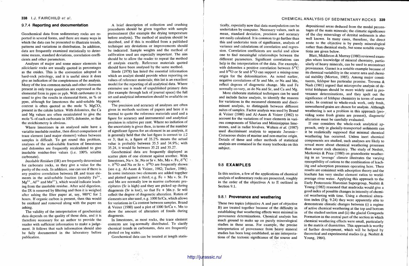
338 I .J . FAIRCHILD ef AL.
9.7A Reporting and documentat ion
Geochemical da ta from sedimentary rocks are reported in several forms, and there are many ways in which the data can be presented to illustrate t rends , pat terns and variations in distribution. In addit ion, data are frequently examined statistically to determine means , s tandard deviations, correlat ion coefficients and other parameters .
Analyses of major and some minor e lements in siliciclastic rocks are usually quoted in percentages as the oxides. This is the convention adopted in hard-rock petrology, and it is useful since it does give an indication of the completeness of the analysis. Many of the less common metals and other elements present in only trace quanti t ies are expressed as the elemental form in ppm or ppb . With carbonates it is usual t o give the results in elemental form, as % or ppm, although for limestones the acid-soluble Mg content is often quoted as the mole % M g C 0 3
present in the calcite lattice. With dolomites , the Ca and Mg values are often recalculated to give the mole % of each carbonate in 100% dolomite , so that the stoichiometry is obvious.
Where limestones in an analysed suite have a variable insoluble residue, then direct comparison of trace element (and major e lement) values between samples is difficult. To get round this p roblem, analyses of the acid-soluble fraction of limestones and dolomites are frequently recalculated to give insoluble residue-free values (i .e. 100% soluble carbonate) .
Insoluble Residues ( IR) are frequently determined for carbonate rocks, as they give a value for the purity of the rock. In addit ion, one can see if there is any positive correlation between I R and trace elements in the acid-soluble fraction (notably F e 2 + , M g 2 + , A l 3 + and M n 2 + ) , which would indicate leaching from the insoluble residue. After acid digestion, the IR is removed by filtering and then it is weighed after ashing the filter paper at, say, 900°C for 2 hours . If organic carbon is present , then this would be oxidized and removed along with the paper on ashing.
The validity of the interpretat ion of geochemical data depends on the quality of those data , and it is therefore necessary for an author to provide the reader with sufficient information to make a judgement . It follows that such information should also be fully documented in the laboratory before publication.
A brief description of collection and crushing procedures should be given together with sample pre t rea tment (for example the drying tempera ture before analysis). The method of analysis should be decribed, and if this is modified from a published technique any deviations o r improvements should be indicated. Sample weights and the method of calibration used are especially important . T h e aim should be to allow the reader to repeat the method of analysis exactly. Reference materials quoted should have been analysed by the same method .
Steele (1978) has listed the essential information which an analyst should provide when report ing on values of reference materials; this list is an excellent model for the report ing of all analytical data . W h e r e extensive use is m a d e of unpublished primary data (for example through lack of journal space) the full set and analytical information should be available on request .
The precision and accuracy of analyses are often given in methods sections of papers and here it is normal to quote the reference materials used and a figure for accuracy and instrumental and analytical precision in relative per cent. Where no indiation of the uncertainty is given then , in terms of the number of significant figures for an e lement in an analysis, it is generally held that the last figure is correct to ± 2 or 3 ; that is, a figure of 35 .2% means the actual value is probably between 35.5 and 3 4 . 9 % ; with 35.24, it would lie between 35.21 and 35.27.
Geochemical data are frequently displayed as scatter plots of one element against another . With l imestones, Na v. Sr, Na or Sr v. Mn , Mn v. F e , 5 1 3 C v. 8 1 8 0 and Na or Sr v. 8 1 8 0 are frequently shown (see e.g. Al-Aasm & Veizer, 1982; Tucker , 1986). In some instances two elements are added together and plotted against a third; e.g. Fe + Mn v. Sr. Fe and Mn are normally low in marine carbonate precipitates (Sr is high) and they are picked u p during diagenesis (Sr is lost), so that Fe + Mn,<y. Sr will reflect the degree of diagenetic alteration. Rat ios of elements are also used, e.g. 1000 Sr/Ca, which allows for variations in Ca content between samples. Brand & Veizer (1980) used a plot of 1000 Sr/Ca v. Mn to show the amount of alteration of fossils during diagenesis.
In l imestones, as most rocks, the trace element contents are log-normally distributed. To clarify chemical t rends in carbonates , data are frequently plotted on log scales.
Geochemical data can be t reated at length statis-
CHEMICAL ANALYSIS OF SEDIMENTARY ROCKS 339
tically, especially now that data manipulation can be under taken by computer . Necessary values, such as mean , standard deviation, precision and accuracy are easily calculated. It is common to go further than this and under take tests of significance, analysis of variance and calculations of correlation and regression. Correlat ion coefficients are useful and allow one to find meaningful relationships between the different parameters . Significant correlations can help in the interpretat ion of the data . For example, with dolomites a positive correlation between 5 1 3 C and 8 l s O or Sr and 8 1 3 0 can support a mixing-zone origin for t he dolomitization. As noted earlier, negative correlations of Sr and Mn, or Na and Mn, reflect degrees of diagenetic change. Mn and Fe normally co-vary, as do Na and Sr, and Ca and Mg.
More e laborate statistical techniques can be used and include factor analysis, to identify the reasons for variations in the measured elements and discriminant analysis, to distinguish be tween different suites of samples. Factor analysis was used by Brand & Veizer (1980) and Al-Aasm & Veizer (1982) to account for the variations of t race elements in various components of Silurian and Mississippian limestones, and in rudist bivalves. Wal te rs et al. (1987) used discriminant analysis to separate J u r a s s i c -Cretaceous shales of marine and non-marine origin. Details of these and other methods of statistical analysis are contained in the many textbooks on this subject.
9.8 E X A M P L E S
In this section, a few of the applications of chemical analysis of sedimentary rocks are presented, roughly in the order of the objectives A to E outlined in Section 9 .1 .
9.8.1 Provenance and weathering
These two topics (objective A and part of objective B) are t rea ted together because of the difficulty in establishing that weathering effects were minimal in provenance determinat ions . Chemical analysis has much ground to make up on purely mineralogical studies in these areas . For example , the precise interpretat ion of provenance f rom heavy mineral studies has been long established, as are interpretations of the tectonic significance of the source and
depositional areas deduced from the modal percentages of the main minerals; the climatic significance of the clay mineralogy of detrital sediments is also well known. In many cases, therefore, the direct route to the objective is by purely mineralogical ra ther than chemical study, but some notable exceptions are given below.
Blatt , Middleton & Murray (1980) reviewed examples where knowledge of mineral chemistry, particularly of heavy minerals , can be used to reconstruct provenance . G a r n e t is a notable example because of its chemical variability in the source area and chemical stability (Mor ton , 1985). A m o n g major constituents , feldspar has particular promise. Trevena & Nash (1981) argued that microprobe analysis of detrital feldspars should be more widely used in provenance determinat ions , and they spelt out the significance of feldspar chemistry in terms of source rocks. In contrast to whole-rock work, only fresh, unweathered grains are chosen for analysis. Although weathering is not a problem in this approach ( p r o - /
viding some fresh grains are present ) , diagenetic 7
alterat ion must be carefully evaluated. If o n e considers t he whole-rock analytical ap
proach, only in glacially-transported sediments can it b e realistically supposed that minimal chemical weathering has occurred. Unless inert chemical components are studied, such analyses are likely to reveal more about chemical weathering processes than source rock chemistry. The study of Nesbitt , Markovics & Price (1980) on granodiori te weathering in an 'average ' climate illustrates the varying susceptibility of cations to the combinat ion of leaching and adsorption processes operating here . Their results are consistent with adsorption theory and the leachate has very similar e lement ratios to world-average river water . Applying this approach to the Early Proterozoic Huronian Supergroup, Nesbitt & Y o u n g (1982) reasoned tha t mudrocks would give a good index of possible changes in intensity of chemical weather ing with t ime. Using a chemical alteration index (Fig. 9.24) they were apparently able to demonst ra te climatic changes between (i) a regime of active chemical weathering at the top and bot tom of the studied section and (ii) the glacial Gowganda Format ion in the central par t of the section in which chemical weather ing effects were small, particularly in the matrix of diamictites. This approach is worthy of further development , which will be helped by theoretical and exper imental studies (e .g. Nesbit t & Young , 1984).
http://jurassic.ru/
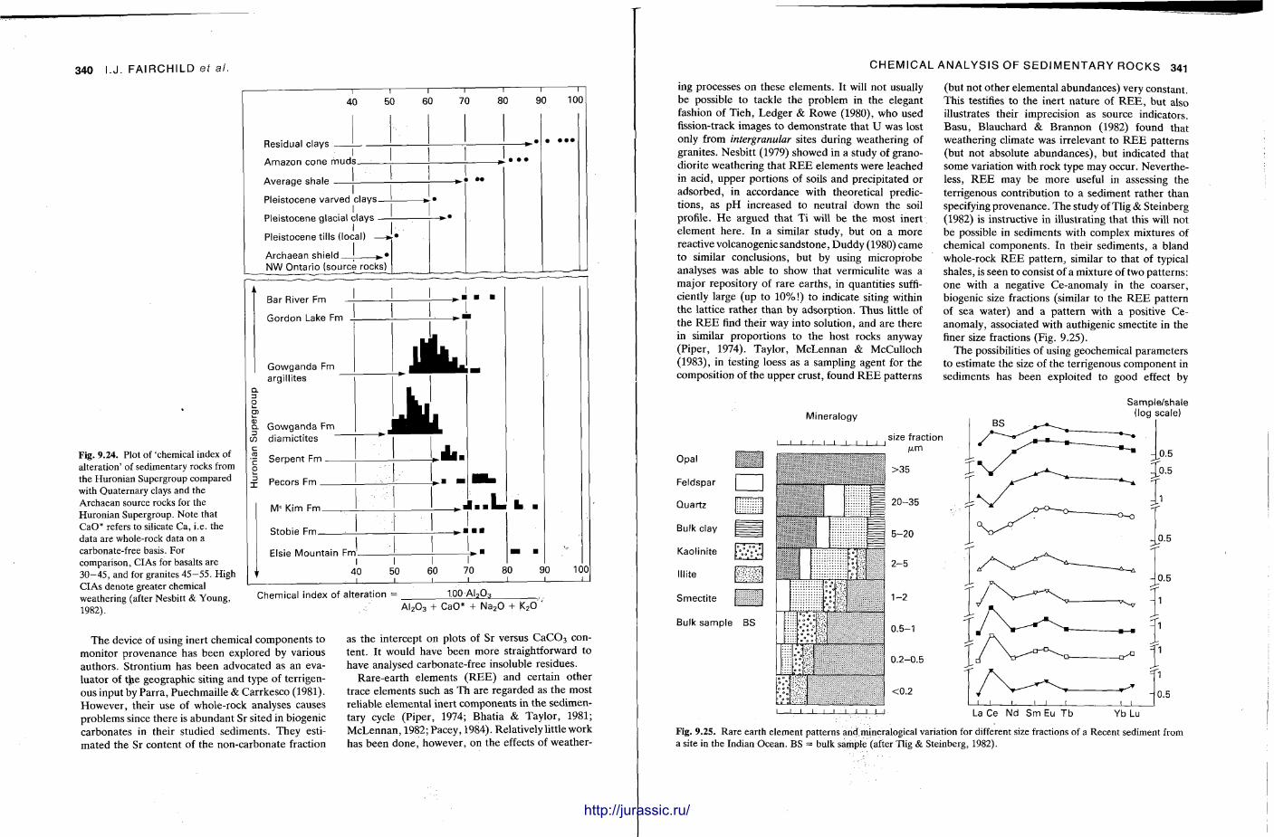
340 I.J. FAIRCHILD ef al.
Fig. 9.24. Plot of 'chemical index of alteration' of sedimentary rocks from the Huronian Supergroup compared with Quaternary clays and the Archaean source rocks for the Huronian Supergroup. Note that CaO* refers to silicate Ca, i.e. the data are whole-rock data on a carbonate-free basis. For comparison, CIAs for basalts are 3 0 - 45, and for granites 45-55 . High CIAs denote greater chemical weathering (after Nesbitt & Young, 1982).
Residual clays _
Amazon cone muds
Average shale _
Pleistocene varved clays I
Pleistocene glacial clays I
Pleistocene tills (loca
Archaean shield. NW Ontario (source rocks)
Bar River Fm
Gordon Lake Fm
Chemical index of alteration = 1.00 AI 2 Q 3
A l , 0 3 + CaO* Na 2 0 + K 2 0
The device of using inert chemical components to moni tor provenance has been explored by various authors . Strontium has been advocated as an eva-luator of the geographic siting and type of terrigenous input by Parra , Puechmaille & Carrkesco (1981). However , their use of whole-rock analyses causes problems since there is abundan t Sr sited in biogenic carbonates in their studied sediments . They estimated the Sr content of the non-carbonate fraction
as the intercept on plots of Sr versus C a C 0 3 content . It would have been more straightforward to have analysed carbonate-free insoluble residues.
Rare-ear th elements ( R E E ) and certain o ther t race elements such as Th are regarded as the most reliable elemental inert components in the sedimentary cycle (Piper, 1974; Bhatia & Taylor , 1981; McLennan , 1982; Pacey, 1984). Relatively little work has been done , however , on the effects of weather-
CHEMICAL ANALYSIS OF SEDIMENTARY ROCKS 341
ing processes on these elements . It will not usually be possible to tackle the problem in the elegant fashion of Tieh, Ledger & Rowe (1980), who used fission-track images t o demons t ra te tha t U was lost only from intergranular sites during weathering of granites. Nesbit t (1979) showed in a study of grano-diorite weathering that R E E elements were leached in acid, upper port ions of soils and precipitated or adsorbed, in accordance with theoretical predict ions, as p H increased to neutral down the soil profile. H e argued that Ti will be the most inert e lement here . In a similar study, but on a more reactive volcanogenic sandstone, Duddy (1980) came to similar conclusions, but by using microprobe analyses was able to show that vermiculite was a major repository of rare ear ths , in quantit ies sufficiently large (up to 10%!) to indicate siting within the lattice ra ther than by adsorption. Thus little of the R E E find their way into solution, and are there in similar propor t ions to t he host rocks anyway (Piper, 1974). Taylor, McLennan & McCulIoch (1983), in testing loess as a sampling agent for the composit ion of the upper crust, found R E E pat terns
Mineralogy
i — i i — i i i i i i i i
(but not o ther elemental abundances) very constant. This testifies to the inert nature of R E E , but also illustrates their imprecision as source indicators. Basu, Blauchard & Brannon (1982) found that weathering climate was irrelevant to R E E patterns (but not absolute abundances) , but indicated that some variation with rock type may occur. Nevertheless, R E E may be more useful in assessing the terrigenous contr ibution to a sediment ra ther than specifying provenance. The study of Tlig & Steinberg (1982) is instructive in illustrating that this will not be possible in sediments with complex mixtures of chemical components . In their sediments , a bland whole-rock R E E pat tern , similar to that of typical shales, is seen to consist of a mixture of two pat terns: one with a negative Ce-anomaly in the coarser, biogenic size fractions (similar to the R E E pat tern of sea water) and a pa t te rn with a positive Ce-anomaly, associated with authigenic smectite in the finer size fractions (Fig. 9.25).
T h e possibilities of using geochemical parameters to est imate the size of the terr igenous component in sediments has been exploited to good effect by
Sample/shale (log scale)
Opal
Feldspar
Quartz
Bulk clay
Kaolinite
Illite
Smectite
Bulk sample BS
size fraction /xm
>35
20-35
5-20
2-5
1-2
0.5-1
0.2-0.5
<0.2
La Ce Nd Sm Eu Tb Yb Lu
Fig. 9.25. Rare earth element patterns and mineralogical variation for different size fractions of a Recent sediment from a site in the Indian Ocean. BS = bulk sample (after Tlig & Steinberg, 1982).
Hit http://jurassic.ru/
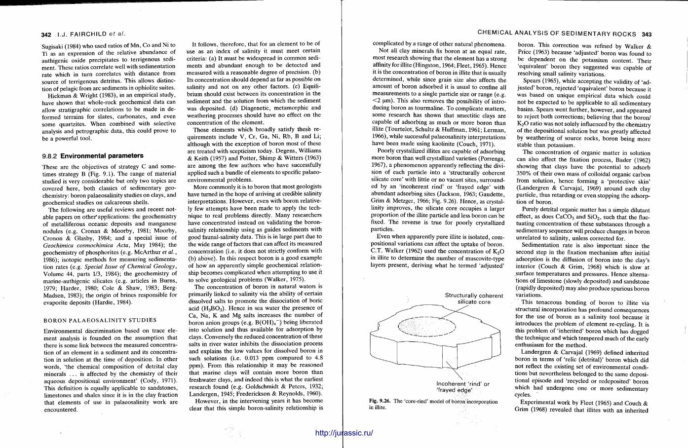
342 I.J. FAIRCHILD et al. It follows, therefore, that for an element to be of
use as an index of salinity it must meet certain criteria: (a) It must be widespread in common sediments and abundant enough to be detected and measured with a reasonable degree of precision, (b) Its concentrat ion should depend as far as possible on salinity and not on any other factors, (c) Equilibr ium should exist between its concentrat ion in the sediment and the solution from which the sediment was deposited, (d) Diagenet ic , metamorphic and weathering processes should have n o effect on the concentrat ion of the e lement .
Those elements which broadly satisfy these- requirements include V , Cr, G a , Ni , R b , B and Li; al though with the exception of boron most of these are t reated with scepticism today. Degens , Williams & Keith (1957) and Pot ter , Shimp & Wit ters (1963) are among the few authors who have successfully applied such a bundle of e lements to specific palaeo-environmental problems.
More commonly it is to boron that most geologists have turned in the hope of arriving at credible salinity interpretat ions. However , even with boron relatively few at tempts have been m a d e to apply the technique to real problems directly. Many researchers have concentrated instead on validating the boron-salinity relationship using as guides sediments with good faunal-salinity data . This is in large par t due to the wide range of factors that can affect its measured concentrat ion (i .e. it does not strictly conform with (b) ' above) . In this respect boron is a good example of how" an apparently simple geochemical relationship becomes complicated when at tempting to use it to solve geological problems (Walker , 1975).
T h e concentrat ion of boron in natural waters is primarily l inked to salinity via the ability of certain dissolved salts to p romote the dissociation of boric acid (H3BO3). Hence in sea water the presence of Ca , N a , K and Mg salts increases the number of boron anion groups (e.g. B ( O H ) 4 ~ ) being liberated into solution and thus available for adsorption by clays. Conversely the reduced concentrat ion of these salts in river water inhibits the dissociation process and explains the low values for dissolved boron in such solutions ( i .e . 0.013 ppm compared to 4.8 p p m ) . F rom this relationship it may be reasoned that marine clays will contain more boron than freshwater clays, and indeed this is wha t the earliest research found (e.g, Goldschmidt & Peters , 1932; Landergen , 1945; Frederickson & Reynolds , 1960).
However , in the intervening years it has become clear that this simple boron-salinity relationship is
CHEMICAL ANALYSIS OF SEDIMENTARY ROCKS 343
complicated by a range of o ther natural phenomena . N o t all clay minerals fix boron at an equal ra te ,
most research showing that the element has a strong affinity for illite (Hingston, 1964; Fleet , 1965). H e n c e it is the concentrat ion of boron in illite that is usually de termined , while since grain size also affects the amount of boron adsorbed it is usual to confine all measurements to a single particle size or range (e .g. < 2 um) . This also removes the possibility of introducing boron as tourmaline. T o complicate mat te rs , some research has shown that smectitic clays are capable of adsorbing as much or more boron than illite (Tourtelot , Schultz & Huffman, 1961; Le rman , 1966), while successful palaeosalinity interpretat ions have been made using kaolinite (Couch, 1971).
Poorly crystallized illites are capable of adsorbing more boron than well crystallized varieties (Porrenga, 1967), a phenomenon apparent ly reflecting the division of each particle into a 'structurally coherent silicate core ' with little or no vacant sites, surrounded by an ' incoherent r ind ' or 'frayed edge ' with abundant adsorbing sites (Jackson, 1963; Gaude t t e , Grim & Metzger, 1966; Fig. 9.26). Hence , as crystallinity improves, the silicate core occupies a larger propor t ion of t he illite particle and less boron can be fixed. The reverse is t rue for poorly crystallized particles.
Even when apparent ly pure illite is isolated, compositional variat ions can affect the up t ake of boron . C.T. Walker (1962) used the concentrat ion of K 2 0 in illite to determine the number of muscovite-type layers present , deriving what he termed 'adjusted'
Structurally coherent silicate core
Incoherent 'rind' or 'frayed edge'
Fig. 9.26. The 'core-rind' model of boron incorporation in illite.
boron. This correction was refined by Walker & Price (1963) because 'adjusted ' boron was found to b e dependen t on t he potassium content . Thei r 'equivalent ' boron they suggested was capable of resolving small salinity variations.
Spears (1965), while accepting the validity of 'adjusted ' boron , rejected 'equivalent ' boron because it was based on unique empirical data which could not be expected to be applicable to all sedimentary basins. Spears went further, however , and appeared to reject both corrections; believing that the boron/ K 2 0 ratio was not solely influenced by the chemistry of the depositional solution but was greatly affected by weathering of source rocks, boron being more stable than potassium.
The concentrat ion of organic mat ter in solution can also affect the fixation process, Bader (1962) showing tha t clays have the potent ial t o adsorb 350% of their own mass of colloidal organic carbon from solution, hence forming a 'protective skin' (Landergren & Carvajal , 1969) around each clay particle, thus re tarding or even stopping the adsorption of boron.
Purely detrital organic matter has a simple dilutant effect, as does C a C 0 3 and S i 0 2 , such that the fluctuating concentrat ion of these substances through a sedimentary sequence will produce changes in boron unrelated to salinity, unless corrected for.
Sedimentat ion rate is also important since the second step in the fixation mechanism after initial adsorption is the diffusion of boron into the clay's interior (Couch & Gr im, 1968) which is slow at surface tempera tures and pressures. Hence alternations of l imestone (slowly deposi ted) and sandstone (rapidly deposi ted) may also p roduce spurious bo ron variations.
This tenaceous bonding of boron to illite via structural incorporation has profound consequences for the use of boron as a salinity tool because it introduces the problem of e lement re-cycling. It is this problem of ' inheri ted ' boron which has dogged the technique and which tempered much of the early enthusiasm for the method .
Landergren & Carvajal (1969) defined inherited boron in terms of 'relic (detr i tal) ' boron which did not reflect the existing set of environmental conditions but nevertheless belonged to the same deposit ional episode and 'recycled or redeposi ted ' boron which had undergone one or more sedimentary cycles.
Exper imental work by Fleet (1965) and Couch & Gr im (1968) revealed that illites with an inherited
Sugisaki (1984) who used ratios of Mn , Co and Ni to Ti as an expression of the relative abundance of authigenic oxide precipitates to terr igenous sediment . These ratios correlate well with sedimentat ion rate which in turn correlates with distance from source of terr igenous detr i tus. This allows distinction of pelagic from arc sediments in ophiolite suites.
Hickman & Wright (1983), in an empirical study, have shown that whole-rock geochemical da ta can allow stratigraphic correlations to be made in deformed terrains for slates, carbonates , and even some quartzites. When combined with selective analysis and petrographic da ta , this could prove to be a powerful tool.
9.8.2 Environmental parameters
These are the objectives of strategy C and sometimes strategy B (Fig. 9.1). The range of material studied is very considerable but only two topics are covered here , both classics of sedimentary geochemistry: boron palaeosalinity studies on clays, and geochemical studies on calcareous shells.
The following are useful reviews and recent notable papers on other* applications: the geochemistry of metalliferous oceanic deposits and manganese nodules (e.g. Cronan & Moorby , 1981; Moorby , Cronon & Glasby, 1984; and a special issue of Geochimica cosmochimica Acta, May 1984); the geochemistry of phosphori tes (e.g. McAr thu r et al., 1986); isotopic methods for measuring sedimentation rates (e.g. Special Issue of Chemical Geology, Volume 44, parts 1/3, 1984); the geochemistry of marine-authigenic silicates (e .g. articles in Burns , 1979; Ha rde r , 1980; Cole & Shaw, 1983; Berg-Madsen , 1983); the origin of brines responsible for evapori te deposits (Hard ie , 1984).
B O R O N P A L A E O S A L I N I T Y S T U D I E S
Environmenta l discrimination based on trace element analysis is founded on the assumption that there is some link between the measured concentration of an element in a sediment and its concentration in solution at the t ime of deposit ion. In other words , ' the chemical composition of detrital clay minerals . . . is affected by the chemistry of their aqueous depositional environment ' (Cody, 1971). This definition is equally applicable to sandstones, l imestones and shales since it is in the clay fraction that e lements of use in palaeosalinity work a re encountered.
http://jurassic.ru/
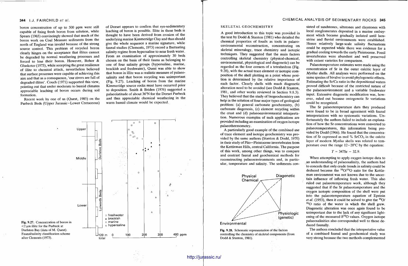
344 I.J. FAIRCHILD ef al.
boron concentrat ion of up to 500 ppm were still capable of fixing fresh boron from solution, while Spears (1965) convincingly showed that much of the boron work on Coal Measure sediments from the north of England was invalid because of the strong source control . This problem of recycled boron clearly hinges on the acceptance that illites cannot be degraded by normal weathering processes and forced to lose their boron . However , Bohor & Gluskoter (1973), while accepting the great resilience of illite to chemical at tack, nevertheless believed that surface processes were capable of achieving this aim and that as a consequence, 'our rivers are full of degraded illites'. Couch (1971) supported this view, pointing out that under modera te to humid climates appreciable leaching of boron occurs during soil formation.
Recent work by one of us (Ques t , 1985) on the Purbeck Beds (Upper Jurassic—Lower Cretaceous)
of Dorse t appears to confirm that syn-sedimentary leaching of boron is possible. Illite in these beds is thought to have been derived from erosion of the underlying marine Kimmeridge Clay and thus should give the whole sequence a marine s ignature, while faunal studies (Clements , 1973) record a fluctuating salinity regime from hypersaline to near fresh water . From an examination of approximately 30 beds chosen on the basis of their fauna as belonging to one of four salinity groups (hypersaline, mar ine , brackish and freshwater) , Ques t was able to show that boron in illite was a realistic measure of palaeosalinity and that boron recycling was un impor tan t (Fig. 9.27). Leaching of boron from the mar ine Kimmeridge source rocks must have occurred prior to deposit ion. Smith & Briden (1976) suggested a palaeolat i tude of about 36°N for the Dorse t Purbeck and thus appreciable chemical weather ing in the warm humid climate would be expected.
Upper
Middle
Lower
Fig. 9.27. Concentration of boron in <2 um illite for the Purbeck at Durlston Bay (data of M. Quest). Faunal/salinity classification scheme after Clements (1973).
freshwater brackish marine hypersaline
120 m total
100 200 300 400 ppm
CHEMICAL ANALYSIS OF SEDIMENTARY ROCKS 345
S K E L E T A L G E O C H E M I S T R Y
A good introduction to this topic was provided in t he text by D o d d & Stanton (1981) w h o detailed t he chemical propert ies of fossils as tools in palaeo-environmental reconstruct ion, concentrat ing on skeletal mineralogy, trace chemistry and isotopic techniques. They suggested that the main factors controlling skeletal chemistry (physical-chemical, environmental , physiological and diagenetic) can be regarded as the four corners of a te t rahedron (Fig. 9.28), with the actual trace e lement or isotopic composition of the shell plotting as a point whose position is determined by the relative impor tance of each factor. Clearly shells with much diagenetic al terat ion need to be avoided (see D o d d & Stanton , 1981, and other works reviewed in Section 9.8.3). They believed that the study of biogeochemistry can help in the solution of four major types of geological problem: (a) general carbonate geochemistry, (b) carbonate diagenesis, (c) e lement recycling within the crust and (d) palaeoenvironmental interpretation. Numerous examples of such applications are provided including an examination of oxygen isotope pa laeothermometry .
A particularly good example of the combined use
of trace e lement and isotope geochemistry was pro
vided by the same authors (Stanton & D o d d , 1970)
in their study of Plio—Pleistocene invertebrates from
the Ket t leman Hills, central California. The purpose
of this work, among other things, was to compare
and contrast faunal and geochemical methods for
reconstructing palaeoenvironments and, in partic
ular, t empera ture and salinity. The sediments con-
Physical Diagenetic
Environmental
Fig. 9.28. Schematic representation of the factors controlling the chemistry of skeletal components (from Dodd & Stanton, 1981).
sisted of sandstones, siltstones and claystones with local conglomerates deposited in a marine embay-ment which became gradually isolated until lacustrine and fluvial environments were established. Hence relatively large-scale salinity fluctuations could be expected while there was evidence for a gradual cooling towards the early Pleistocene. Fossil invertebrates were abundant and well preserved with extant varieties for comparison.
Pa laeotempera ture estimates were made using the concentrat ion of Sr in the outer calcitic layer of Mytilus shells. All analyses were performed on the same species of bivalve to avoid phylogenetic effects. Estimating the Sr/Ca ratio in the depositional waters proved difficult because of the restricted nature of the palaeoenvironment and a variable freshwater input. Extensive diagenetic modification was , however, ruled out because ontogenetic Sr variations could be recognized.
T h e Sr pa laeotempera ture da ta they produced were found to be in broad agreement with faunal interpretat ions with no systematic variations. Unfortunately the authors failed to include an explanation of how the Sr concentrat ions were converted to pa laeotempera tures , this information being provided by D o d d (1966). H e found that the concentration of Sr expressed as mol % S r C 0 3 in the calcite layer of modern Mytilus shells was related to tempera ture over the range 12—20°C by the equation:
T = 347Sr - 32.9.
When at tempting to apply oxygen isotope data to an understanding of palaeosalinity, the authors had to concede that only crude t rends in salinity could be deduced because the 1 8 0 / 1 6 0 rat io for the Kett le-man environment was not known due to the uncertain influence of inflowing fresh water . This also ruled out pa laeotempera ture work, al though they suggested that if the Sr pa laeotempera ture and the oxygen isotopic composit ion of the shell were put into the pa laeotempera ture equat ion of Epstein et al. (1953), then it could be solved to give the 1 8 0 / 1 5 0 ratio of the water in which the shell grew. Diagenetic alteration was once again found to be unimpor tant due to the lack of any significant lightening of the measured 5 1 8 0 values. Oxygen isotope palaeosalinities also corresponded well to those deduced faunally.
The authors concluded that the interpretative value of a combined faunal and geochemical study was very strong because the two methods complemented
http://jurassic.ru/
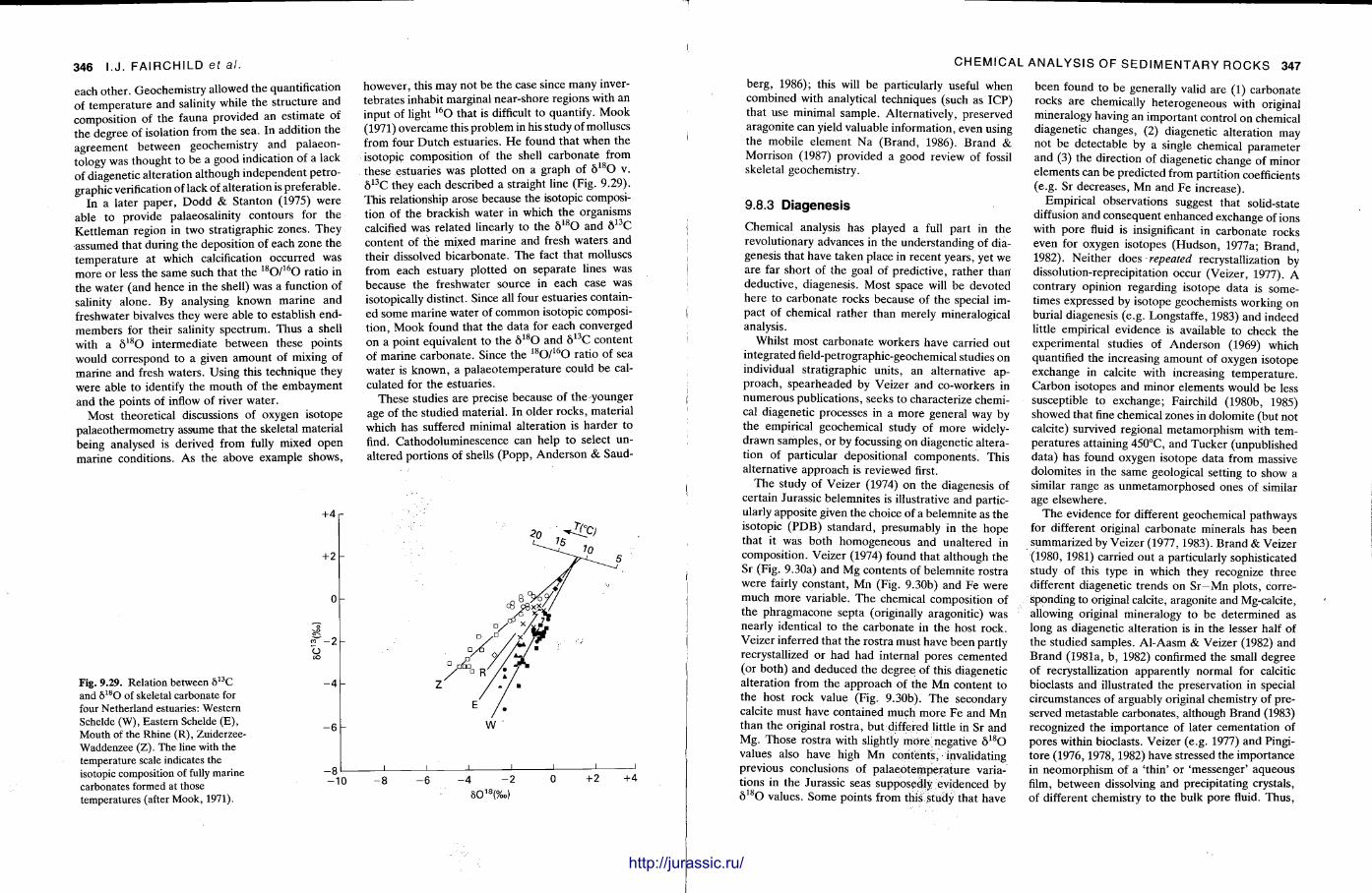
346 I .J . FAIRCHILD ef al.
each other . Geochemist ry allowed the quantification of t empera ture and salinity while the structure and composition of the fauna provided an est imate of the degree of isolation from the sea. In addition the agreement between geochemistry and palaeontology was thought to be a good indication of a lack of diagenetic alteration although independent petrographic verification of lack of alteration is preferable.
In a later paper , D o d d & Stanton (1975) were able to provide palaeosalinity contours for the Ket t leman region in two stratigraphic zones. They -assumed that during the deposition of each zone the t empera tu re at which calcification occurred was more or less the same such that the 1 8 0 / 1 6 0 ratio in the water (and hence in the shell) was a function of salinity alone. By analysing known marine and freshwater bivalves they were able to establish end-members for their salinity spectrum. Thus a shell with a 5 1 8 0 intermediate between these points would correspond t o a given amoun t of mixing of marine and fresh waters . Using this technique they were able to identify the mouth of the embayment and the points of inflow of river water .
Most theoretical discussions of oxygen isotope palaeothermometry assume that the skeletal material being analysed is derived from fully mixed open mar ine condit ions. As the above example shows,
+ 4 r
+ 2 h
0 -
o -VP cr--
p~-2 -o t o
Fig. 9.29. Relation between 5 1 3 C - 4 _ and 6 l s O of skeletal carbonate for four Netherland estuaries: Western Schelde (W), Eastern Schelde (E), _ g _ Mouth of the Rhine (R), Zuiderzee-Waddenzee (Z). The line with the temperature scale indicates the isotopic composition of fully marine — 8 '— carbonates formed at those ~~ ̂ ̂ temperatures (after Mook, 1971).
however , this may not be the case since many invertebrates inhabit marginal near-shore regions with an input of light 1 6 0 that is difficult to quantify. Mook (1971) overcame this problem in his study of molluscs from four Dutch estuaries. H e found that when the isotopic composit ion of the shell carbonate from these estuaries was plotted on a graph of 5 1 8 0 v. 5 1 3 C they each described a straight line (Fig. 9.29). This relationship arose because the isotopic composition of the brackish water in which the organisms calcified was related linearly to the 8 l s O and 8 1 3 C content of the mixed mar ine and fresh waters and their dissolved bicarbonate . T h e fact that molluscs from each estuary plot ted on separate lines was because the freshwater source in each case was isotopically distinct. Since all four estuaries contained some marine water of common isotopic composit ion, Mook found that the data for each converged on a point equivalent to the 8 1 8 0 and 8 1 3 C content of marine carbonate . Since the 1 8 0 / 1 6 0 ratio of sea water is known, a pa laeotempera ture could be calculated for the estuaries.
These studies are precise because of the younger age of the studied material . In older rocks, material which has suffered minimal alteration is harder to find. Cathodoluminescence can help to select unaltered port ions of shells (Popp , Anderson & Saud-
i i i i i 1 1
- 8 - 6 - 4 - 2 0 +2 + 4 501 8(%o)
CHEMICAL ANALYSIS OF SEDIMENTARY ROCKS 347 berg, 1986); this will be particularly useful when combined with analytical techniques (such as ICP) that use minimal sample. Alternatively, preserved aragonite can yield valuable information, even using the mobile e lement Na (Brand, 1986). Brand & Morrison (1987) provided a good review of fossil skeletal geochemistry.
9.8.3 Diagenesis
Chemical analysis has played a full part in the revolutionary advances in the understanding of diagenesis tha t have taken place in recent years, yet we are far short of the goal of predictive, ra ther than deduct ive, diagenesis. Most space will b e devoted here to carbonate rocks because of the special impact of chemical ra ther than merely mineralogical analysis.
Whilst most carbonate workers have carried out integrated field-petrographic-geochemical studies on individual stratigraphic units, an alternative approach, spearheaded by Veizer and co-workers in numerous publications, seeks to characterize chemical diagenetic processes in a more general way by the empirical geochemical study of more widely-drawn samples , or by focussing on diagenetic alteration of particular depositional components . This alternative approach is reviewed first.
The study of Veizer (1974) on the diagenesis of certain Jurassic belemnites is illustrative and particularly apposite given the choice of a belemnite as the isotopic (PDB) s tandard, presumably in the hope that it was both homogeneous and unaltered in composit ion. Veizer (1974) found that al though the Sr (Fig. 9.30a) and Mg contents of belemnite rostra were fairly constant , Mn (Fig. 9.30b) and Fe were much m o r e variable. T h e chemical composition of the phragmacone septa (originally aragonitic) was nearly identical t o t he carbonate in t he host rock. Veizer inferred that the rostra must have been partly recrystallized or had had internal pores cemented (or both) and deduced the degree of this diagenetic alteration from the approach of the M n content to the host rock value (Fig. 9.30b). T h e secondary calcite must have contained much more Fe and Mn than the original rostra , but differed little in Sr and Mg. Those rostra with slightly more negative 8 1 8 0 values also have high M n contents , invalidating previous conclusions of pa laeotempera ture variat ions in t he Jurassic seas supposedly evidenced by 8 1 8 0 values. Some points from this study that have
been found to be generally valid are (1) carbonate rocks a re chemically heterogeneous with original mineralogy having an important control on chemical diagenetic changes, (2) diagenetic alteration may not be detectable by a single chemical parameter and (3) the direction of diagenetic change of minor e lements can be predicted from parti t ion coefficients (e.g. Sr decreases, M n and Fe increase).
Empirical observations suggest that solid-state diffusion and consequent enhanced exchange of ions with pore fluid is insignificant in carbonate rocks even for oxygen isotopes (Hudson, 1977a; Brand, 1982). Neither does repeated recrystallization by dissolution-reprecipitation occur (Veizer, 1977). A contrary opinion regarding isotope da ta is sometimes expressed by isotope geochemists working on burial diagenesis (e.g. Longstaffe, 1983) and indeed little empirical evidence is available t o check the experimental studies of Anderson (1969) which quantified the increasing amount of oxygen isotope exchange in calcite with increasing tempera ture . Carbon isotopes and minor elements would be less susceptible to exchange; Fairchild (1980b, 1985) showed that fine chemical zones in dolomite (but not calcite) survived regional metamorphism with tempera tures attaining 450°C, and Tucker (unpublished data) has found oxygen isotope data from massive dolomites in the same geological setting to show a similar range as unmetamorphosed ones of similar age elsewhere.
The evidence for different geochemical pathways for different original carbonate minerals has been summarized by Veizer (1977,1983). Brand & Veizer (1980,1981) carried ou t a particularly sophisticated study of this type in which they recognize three different diagenetic t rends on Sr—Mn plots, corresponding to original calcite, aragonite and Mg-calcite, allowing original mineralogy to be determined as long as diagenetic alteration is in the lesser half of the studied samples. Al -Aasm & Veizer (1982) and Brand (1981a, b , 1982) confirmed the small degree of recrystallization apparent ly normal for calcific bioclasts and illustrated the preservation in special circumstances of arguably original chemistry of preserved metastable carbonates, although Brand (1983) recognized the importance of later cementat ion of pores within bioclasts. Veizer (e.g. 1977) and Pingitore (1976,1978,1982) have stressed the importance in neomorphism of a ' thin ' or 'messenger ' aqueous film, be tween dissolving and precipitating crystals, of different chemistry to the bulk pore fluid. Thus ,
http://jurassic.ru/
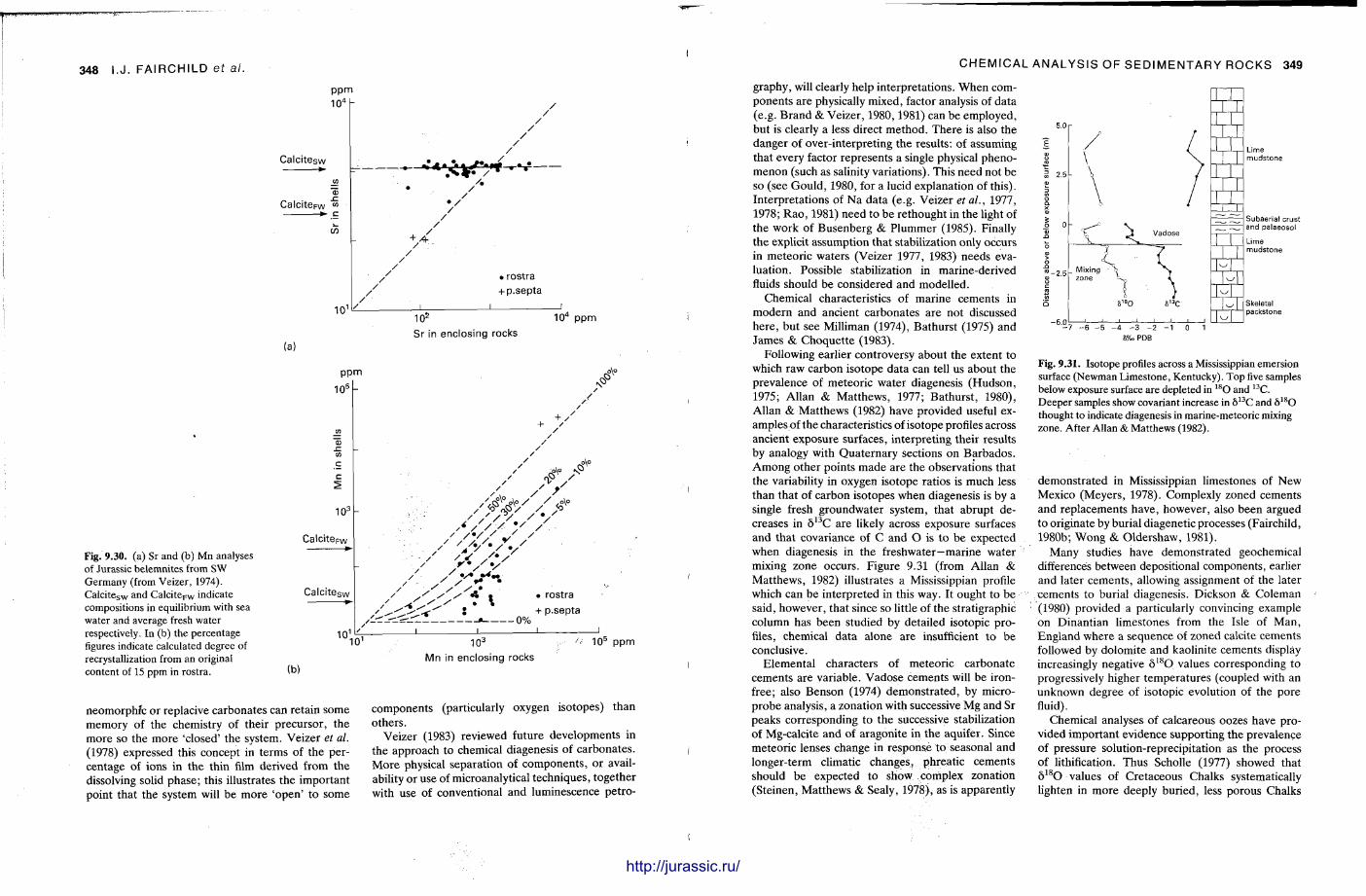
348 I.J. FAIRCHILD e t a l .
10" ppm
Fig. 9.30. (a) Sr and (b) Mn analyses of Jurassic belemnites from SW Germany (from Veizer, 1974). Calc i te s w and Calci te F W indicate compositions in equilibrium with sea water and average fresh water respectively. In (b) the percentage figures indicate calculated degree of recrystallization from an original content of 15 ppm in rostra.
ppm
10 5
c
10 3
Calcite Fw
Calcitesw *~ s / ' t
• / , o \ °
/
< 1 0%
• rostra + p.septa
(b)
10 3
Mn in enclosing rocks 10 5 ppm
neomorphfc or replacive carbonates can retain some memory of the chemistry of their precursor , the more so the more 'closed' the system. Veizer et al. (1978) expressed this concept in terms of the percentage of ions in the thin film derived from the dissolving solid phase; this illustrates the important point that the system will be more 'open ' to some
components (particularly oxygen isotopes) than others .
Veizer (1983) reviewed future developments in the approach to chemical diagenesis of carbonates . M o r e physical separat ion of components , or availability or use of microanalytical techniques, together with use of conventional and luminescence petro-
f
CHEMICAL ANALYSIS OF SEDIMENTARY ROCKS 349
graphy, will clearly help interpretat ions. When components are physically mixed, factor analysis of data (e.g. Brand & Veizer , 1980,1981) can be employed, but is clearly a less direct method . The re is also the danger of over-interpret ing the results: of assuming that every factor represents a single physical phenomenon (such as salinity variations). This need not be so (see Gould , 1980, for a lucid explanation of this). Interpretat ions of Na da ta (e.g. Veizer et al., 1977, 1978; R a o , 1981) need to be re thought in the light of the work of Busenberg & Plummer (1985). Finally the explicit assumption that stabilization only occurs in meteoric waters (Veizer 1977, 1983) needs evaluation. Possible stabilization in marine-derived fluids should be considered and modelled.
Chemical characteristics of marine cements in modern and ancient carbonates are not discussed he re , but see Milliman (1974), Bathurst (1975) and James & Choque t t e (1983).
Following earlier controversy about the extent to which raw carbon isotope data can tell us about the prevalence of meteor ic water diagenesis (Hudson , 1975; Allan & Mat thews, 1977; Bathurst , 1980), Allan & Mat thews (1982) have provided useful examples of the characteristics of isotope profiles across ancient exposure surfaces, interpreting their results by analogy with Quate rnary sections on Barbados . A m o n g other points made are the observations that the variability in oxygen isotope ratios is much less than that of carbon isotopes when diagenesis is by a single fresh groundwater system, that abrupt decreases in 5 1 3 C are likely across exposure surfaces and that covariance of C and O is to b e expected when diagenesis in the freshwater—marine water mixing zone occurs. Figure 9.31 (from Allan & Mat thews, 1982) illustrates a Mississippian profile which can be interpreted in this way. It ought to be said, however, that since so little of the stratigraphic column has been studied by detailed isotopic profiles, chemical data alone are insufficient to be conclusive.
Elementa l characters of meteoric carbonate cements are variable. Vadose cements will be iron-free; also Benson (1974) demonst ra ted , by microprobe analysis, a zonation with successive Mg and Sr peaks corresponding to the successive stabilization of Mg-calcite and of aragonite in the aquifer. Since meteoric lenses change in response to seasonal and longer-term climatic changes, phreatic cements should be expected to show complex zonation (Steinen, Mat thews & Sealy, 1978), as is apparent ly
V a d o s e
M i x i n g • z o n e - 1
8 1 3 C
L i m e m u d s t o n e
S u b a e r i a l c r u s t a n d p a l a e o s o l
L i m e m u d s t o n e
S k e l e t a l p a c k s t o n e
- 7 - 6 - 5 - 4 - 3 - 2 - 1 0 1 8%o PDB
Fig. 9.31. Isotope profiles across a Mississippian emersion surface (Newman Limestone, Kentucky). Top five samples below exposure surface are depleted in l s O and 1 3 C . Deeper samples show covariant increase in 6 1 3 C and 5 l s O thought to indicate diagenesis in marine-meteoric mixing zone. After Allan & Matthews (1982).
demonst ra ted in Mississippian limestones of New Mexico (Meyers , 1978). Complexly zoned cements and replacements have , however , also been argued to originate by burial diagenetic processes (Fairchild, 1980b; Wong & Oldershaw, 1981).
Many studies have demonst ra ted geochemical differences between depositional components, earlier and later cements , allowing assignment of the later cements to burial diagenesis. Dickson & Coleman (1980) provided a particularly convincing example on Dinant ian l imestones from the Isle of Man , England where a sequence of zoned calcite cements followed by dolomite and kaolinite cements display increasingly negative 5 1 8 0 values corresponding to progressively higher tempera tures (coupled with an unknown degree of isotopic evolution of the pore fluid).
Chemical analyses of calcareous oozes have provided impor tant evidence support ing the prevalence of pressure solution-reprecipitation as the process of lithification. Thus Scholle (1977) showed that 5 1 8 0 values of Cretaceous Chalks systematically lighten in more deeply buried, less porous Chalks
http://jurassic.ru/
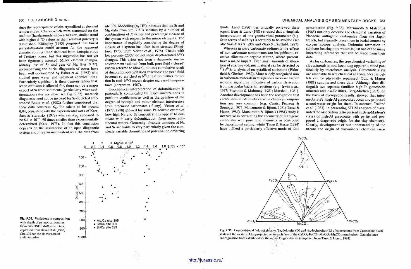
350 I .J . FAIRCHILD ef a l .
since the reprecipitated calcite crystallized at elevated tempera tures . Chalks which were cemented on the seafloor (hardgrounds) show a weaker , similar t rend with higher <5 1 8 0 values as their residual porosity is diminished. Killingley (1983) proposed that burial recrystallization could account for the apparen t climatic cooling t rend deduced from isotopic study of Tert iary oozes, but this suggestion has not yet been rigorously assessed. Minor e lement changes, notably loss of Sr and gain of M g (Fig. 9.32), accompanying the burial diagenesis of oozes have been well documented by Baker et al. (1982) who studied pore water and sediment chemical da ta . Particularly significant is their demonstra t ion that , when diffusion is allowed for, there can be a major export of Sr from sediments (particularly when sedimentat ion rates are slow, see Fig. 9.32); meteoric diagenesis need not be invoked for Sr-depleted limestones! Baker et al. (1982) further considered that their data constrain KSl for calcite to be around 0.04, consistent with the experimental work of Katz , Sass & Starinsky (1972) whereas appeared to be 8.1 x 10~ 4 , 60 times smaller than experimental ly determined (Katz, 1973). In fact this conclusion depends on the assumption of an open diagenetic system and it is also inconsistent with the data from
site 305. Modelling (by IJF) indicates that the Sr and Mg data from site 305 is satisfied by a number of combinations of K values and percentage closure of the system with respect to the minor e lements . T h e impor tance of explicitly considering the degree of closure of a system has often been stressed (Pingitore , 1978, 1982; Veizer et al., 1978). Chalks with low porosity (20%) do not show depth-related 6 l s O changes. This arises not from a diagenetic micro-environment isolated from bulk pore fluid ('closed' system referred to above) , but as a cumulative result of dissolution-precipitation reactions: the pore fluid becomes so enriched in 6 l s O that no further reduction in rock 5 1 8 0 occurs despite increased temperatures (Jorgensen, 1987).
Geochemical interpretat ion of dolomitization is particularly complicated by major uncertainties in parti t ion coefficients as well as the quest ion of the degree of isotopic and minor e lement interference from precursor carbonates (if any) . Veizer et al. (1977', 1978) showed for some Palaeozoic examples how high Na and Sr concentrat ions appear to correlate with early dolomitization from more continental waters . General ly , absolute amounts of Na and Sr a re liable to vary particularly given the complexly variable chemistries of potential dolomitizing
Fig. 9.32. Variations in composition with depth of pelagic carbonates from two DSDP drill sites. Data replotted from Baker et al. (1982). Site 305 has the slower rate of sedimentation.
1 2 3 Mg/Ca x 10 3
0 0.2 0.4 0.6 0.8 1.0 1.2 1.4 1.6 1.8 Sr/Ca x 10 3
100
200
300
400
£ 500
O 600
700
800
900
1000
t r ~ i 1 — A ~ ~ r
• A
A
• Mg/Ca site 305 * Sr/Ca site 305 • Sr/Ca site 289
CHEMICAL ANALYSIS OF SEDIMENTARY ROCKS 351
fluids. Land (1980) has critically reviewed these topics. Bein & Land (1983) stressed that a simplistic interpretat ion of one geochemical parameter (e.g. Sr in terms of salinity) is certainly to be avoided (see also Sass & Katz , 1982 and Z h a o & Fairchild, 1987).
Whereas in pure carbonate sediments the effects of non-carbonate components are insignificant, reactive silicates or organic mat ter , where present , have a major impact . Even small amounts of alteration of reactive volcanic material can be detected by 8 7 S r / 8 6 S r analysis of recrystallized carbonate (Elder-field & Gieskes, 1982). M o r e widely recognized now in carbonate minerals in terr igenous rocks are carbon isotopic signatures indicative of carbon derivation from particular bacterial reactions (e.g. Irwin et al., 1977; Pisciotto & Mahoney , 1981; Marshall , 1981). Ano the r development has been the recognition that carbonates of extremely variable chemical composition are very common (e.g. Curtis , Pearson & Somogyi, 1975; Matsumoto & Iijima, 1981; Tasse & Hesse , 1984). Matsumoto & Iijima's (1981) study is instructive in correlating the chemistry of authigenic carbonates with pore fluid chemistry as controlled by depositional setting, whilst Tasse & Hesse (1984) have utilized a particularly effective m o d e of data
presentat ion (Fig. 9.33). Matsumoto & Matsuhisa (1985) not only describe the elemental variation of Neogene authigenic carbonates from the Japan t rench, but elegantly place them in burial context by oxygen isotope analysis. Dolomi te formation in sulphate-bearing pore waters is just one of the many interesting inferences that can be made from their data .
As for carbonates , the t rue chemical variability of clay minerals is now becoming apparent , aided particularly by microbeam analysis. Glauconitic clays are amenable to wet chemical analyses because pellets can be physically separated: Odin & Mat te r (1981) summarized these data . Al though they distinguish two separate families: high-Fe glauconitic minerals and low-Fe illites, Berg-Madsen (1983), on the basis of microprobe results, showed that inter-media te-Fe , high-Al glauconites occur and proposed a cool-water origin for them. In contrast , Ireland et al. (1983), in present ing S T E M analyses of clays, noted the association (also present in Berg-Madsen 's clays) of high-Al glauconite with pyrite and proposed a diagenetic origin for the clay chemistry. Clearly, development of our understanding of the na ture and origin of clay-mineral chemical varia-
C a C 0 3
Fig. 9.33. Compositional fields of siderite (S), dolomite (D) and rhodochrosites (R) of concretions from Cretaceous black shales of the western Alps projected on toeach face of the CaC0 3 -FeC0 3 TMnC0 3 -MgC03 tetrahedron. Straight lines are regression lines calculated for the most elongated fields (simplified from Tasse & Hesse, 1984).
http://jurassic.ru/
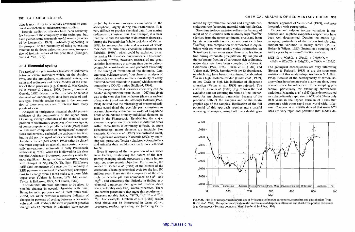
352 I.J. FAIRCHILD ef a l .
tions is most likely to be rapidly advanced by combined microchemical-microstructural studies.
Isotopic studies on silicates have been relatively few because of the complexity of the technique, but have yielded some extremely useful results (reviewed by Longstaffe, 1983). Particularly appealing is the prospect of the possibility of using co-existing minerals to tie down pa laeotempera tures , irrespective of isotopic values of the pore fluid (Elsinger, Savin & Y e h , 1979).
9.8.4 Elemental cycl ing
The geological cycle involves transfer of sediments between several reservoirs which, on the simplest level, are the a tmosphere , continental waters , sea water and sediments and rocks. Models of the kinetics of these processes (e .g. Garre ls & MacKenzie , 1971; Veizer & Jansen, 1979; Berner , Lasaga & Garre ls , 1983) depend on the existence of reliable chemical and mineralogical data from rocks of various ages. Possible secular changes in the composition of these reservoirs are of interest from many points of view.
Analyses of terr igenous material should provide evidence of the composition of the upper crust. Obtaining average est imates of the chemical composition of sedimentary sequences of various ages is, of course , reple te with pitfalls. Schwab (1978) made an extensive compilation of ' terr igenous ' compositions and correctly excluded the carbonate fraction, but he did not disregard other chemical sediments . Ano the r criticism (McLennan , 1982) is that he placed too much emphasis on glacially t ranspor ted , chemically unweathered sediments in early Proterozoic sections (Fig. 9.24). When this is allowed for it is clear that the Archaean—Proterozoic boundary marks the most significant change in the sedimentary record with changes in N a 2 0 / K 2 0 , T h , light REE/heavy R E E (and emergence of a negative E u anomaly in R E E pat terns normalized to chondrites) corresponding to a change from a more mafic to a more felsic upper crust (Veizer & Jansen, 1979; McLennan , Taylor & Eriksson, 1983; McLennan , 1982).
Considerable at tention continues to be given to possible changes in oceanic chemistry with t ime. Being for most purposes and at most times well-mixed, sea water provides a sensitive indicator of changes in pat terns of cycling between other reservoirs and itself. Perhaps the most important putat ive change was an increase in oxidation state accom
panied by increased oxygen accumulation in the a tmosphere , largely during the Proterozoic. It is very difficult to provide chemical data from mar ine sediments to constrain this. For example , it is clear that the Fe and Mn content of dolostones decreased during the Precambrian (whole rock da ta of Veizer , 1978; for microprobe data and a review of whole rock data for pure finely crystalline dolostones see Fairchild, 1980a), which could be explained by an increasing Eh of surface environments . This cannot be readily proven, however , because of the great variation in chemistry at any one t ime due to palaeo-geographic considerat ions, and potential variability in the timing of formation of the dolomite . Less equivocal evidence comes from chemical analyses of palaeosols (and studies on the survivability of easily oxidized detrital minerals in placers) which constrain atmospheric C 0 2 / 0 2 ratios (Hol land, 1984).
T h e proposit ion that seawater chemistry can be t reated in equilibrium terms (Sillen, 1967) has given way to the view that kinetic factors (fluxes in and out of sea water) p redomina te , al though Hol land (1972, 1984) showed that the mineralogy of preserved sediments constrained the possible past excursions in oceanic chemistry within half an order of magni tude limits of abundance of many individual e lements , at least in the Phanerozoic . Establishing the major e lement composit ion of sea water at different t imes within these limits is extremely difficult. In some circumstances, minor elements are tractable. For example ; G r a h a m et al. (1982) demonst ra ted small, but significant variations in oceanic Sr/Ca by analysing well-preserved Tert iary planktonic foraminifera and utilizing their well-known parti t ion coefficient for Sr.
Even if aspects of the composition of sea water were known, establishing the na ture of the temporally-changing kinetic processes is a more important , yet more remote objective. For example , the model of Berner et al. (1983) of the control of the carbonate-silicate geochemical cycle for the last 100 million years illustrates the complexity of the controls on oceanic p H and abundance of C a 2 + and M g 2 + , and conversely the difficulty in finding geochemical parameters that give information about few (preferably only two) kinetic processes. The re are certain parameters that meet this requi rement , however: notably Sr/Ca, 3 4 S / 3 2 S , 1 3 C / 1 2 C and 8 7 Sr / 8 6 S r . For example , Graham et al.'s (1982) results cited above can be interpreted in terms of two processes: seafloor spreading ra te (affecting Ca re-
CHEMICAL ANALYSIS OF SEDIMENTARY ROCKS 353
moved by hydrothermal action) and aragonite precipitation ra te (removing material with high Sr/Ca) .
Strontium isotope variation reflects the balance of input of Sr in solution with relatively high 8 7 S r / 8 6 S r (derived from the upper continental crust) and input by interaction with basaltic oceanic crust (with low 8 7 S r / 8 6 S r ) . The composit ion of carbonates in equilibrium with sea water readily yields information on Sr isotopes in sea water since there is no fractionation during carbonate precipitation. By analysis of the carbonate fraction of carbonate-rich sediments , major data sets have been compiled by Veizer & Compston (1974, 1976), Burke et al. (1982) and Veizer et al. (1983). Samples with low Sr abundance , or which may have been contaminated by abundant 8 7 S r in a high insoluble residue (Burke etal., 1982), or low Ca/Sr or high Mn indicative of diagenetic alteration (Veizer et al., 1983) are rejected. The curve of Burke et al. (1982) (Fig. 9.34) is the best available data set covering the whole of the Phanerozoic for any chemical parameter , because of the precision both of the analyses and of the stratigraphic age of the samples. Realization of the full potential of this approach requires more careful screening of samples, using both the valuable geo
chemical approach of Veizer et al. (1983), and more integration with petrography.
Carbon and sulphur isotope variations in carbonates and sulphate evaporites respectively have been well documented . Despi te the cruder age-grouping, particularly of the carbon isotopic data , antipathetic variation is clearly shown (Veizer, Holser & Wilgus, 1980) illustrating a coupling of C and S cycles by an overall reaction such as:
1 5 C H 2 0 + 8 C a S 0 4 + 2 F e 2 0 3 + 7 M g S i 0 3 = 4 F e S 2 + 8 C a C 0 3 + 7 M g C 0 3 + 7 S i O z + 1 5 H 2 0 .
The geological consequences are very interesting (Berner & Raiswell, 1983) as are the short- term violations of this relationship (Anderson & Ar thur , 1983). Because of the heterogeneity of carbon isotope values in carbonate rocks at any one t ime, there is much scope for refinement of the sampling procedure , particularly for examining shorter- term variations. Magaritz et al. (1983) have demonst ra ted an extraordinarily rapid rise in 5 1 3 C of 8.5%o in only 4000 years in the U p p e r Permian of Texas that correlates with other rapid rises world-wide. Likewise, Claypool et al. (1980) showed that some 5 3 4 S rises are very rapid and postulate that sudden de-
.7100
.7095
.7090
.7085
C/J
%. .7080 CO CO
.7075
.7070
.7065
.7060
y
f t <J
i • '
\ V
qI Tertiary Cretaceous Jurassic Triassic Permian Penn Miss. Devonian Silurian Ordovician Cambrian Pc.
100 200 300 Myr
400 500 600
Fig. 9.34. Plot of Sr isotope variation with age of 744 samples of marine carbonates, evaporites and phosphorites (from Burke et al., 1982). Data points scatter above the line because of diagenetic alteration and short-lived positive excursions (e.g. Cretaceous-Tertiary boundary. Hess, Bender & Schilling, 1986).
1 1 1 1 It
http://jurassic.ru/
354 I.J. FAIRCHILD ef al.
stratification of an ocean basin is the only mechanism that can explain them.
Secular variation in the oxygen isotope composition of carbonates , cherts and phosphori tes takes the form of a progressive decrease in average 6 l s O in older rocks (Veizer & Hoefs , 1976; Knauth & Lowe , 1978; Anderson & Ar thur , 1983). The cause of this variation, whether increased total recrystallization with age, t empera tu re change, or secular variation in seawater isotopic composit ion, is hotly disputed, al though the s t rong buffering of sea water 5 1 8 0 by interaction with new ocean crust is increasingly evident (Holland, 1984). The careful analysis of little-altered port ions of Palaeozoic brachiopod shells (Popp et al., 1986; Veizer , Fritz & Jones ,
1986) demonst ra ted that Palaeozoic sea water was not as isotopically depleted as previously thought . Similarly, Tucker (1986) and Fairchild & Spiro (1987) argued that the average pronounced isotopic depletion in late Proterozoic carbonates relates to mineralogical stabilization rather than changes in oxygen isotopic composit ion of sea water . The alternative approach of using cher t -phosphate pairs to derive both pa laeotempera tures and isotopic composit ions of po re fluids (Karhu & Epste in , 1986) has yielded startlingly high pa laeo tempera tures in Precambrian samples. As so often with the chemical analysis of sedimentary rocks, such interpretat ions cannot be accepted until the mineralogical and petrological history of the analysed samples is well unders tood.
References
Acker, K.L. & Risk, M.J. (1985) Substrate destruction and sediment production by the boring sponge Cliona caribbaea on Grand Cayman Island. / . sedim. Petrol. 55, 705-711.
Adams, A.E., MacKenzie, W.S. & Guildford, C. (1984) Atlas of Sedimentary Rocks under the Microscope. Longmans, London.
Adams, A.E. & Schofield, K. (1983) Recent submarine aragonite, magnesian calcite and hematite cements in a gravel from Islay, Scotland. / . sedim. Petrol. 53, 417-421.
Al-Aasm, I.S. & Veizer, J. (1982) Chemical stabilization of low-Mg calcite: an example of brachiopods. / . sedim. Petrol. 52, 1101-1109
Alexander, L.E. & Klug, H.P. (1948) Basic aspects of X-ray absorption in quantitative diffraction analysis of powder mixtures. Anal. Chem. 20, 886—889
Alexander-Marrack, P.D., Friend, P.F. & Yeats, A.K. (1970) Mark sensing for recording and analysis of sedimentological data. In: Data Processing in Biology and Geology (Ed. by J. Cutbill), pp. 1 — 16. Systematics Association Special Vol. 3. Academic Press, London.
Alexandersson, E.T. (1974) Carbonate cementation in coralline algal nodules in the Skagerrak, North Sea: biochemical precipitation in undersaturated waters. J. sedim. Petrol: 44, 7 -26
Alexandersson, E.T. (1979) Marine maceration of skeletal carbonates in the Skagerrak, North Sea. Sedimentology, 26, 845-852.
Al-Hashimi, W. & Hemingway, J.E. (1974) Recent dolomitization and the origin of the rusty crusts of Northumberland: A reply. / . sedim. Petrol. 44,271—274.
Ali, A.D & Turner, P. (1982) Authigenic K-fe!dspar in the Bromsgrove Sandstone Formation (Triassic) of Central England./, sedim. Petrol. 52, 187-197.
Allan, J. R. & Matthews, R.K. (1977) Carbon and oxygen isotopes as diagenetic and stratigraphic tools: surface and subsurface data, Barbados, West Indies. Geology, 5, 16-20.
Allan, J.R. & Matthews, R.K. (1982) Isotope signatures associated with early meteoric diagenesis. Sedimentology, 29, 791-817.
Allen, D. (1984) A one-stage precision polishing technique for geological specimens. Miner. Mag. 48, 298— 300.
Allen, G. P. (1971) Relationship between grain size distribution and current patterns in the Gironde estuary (France). / . sedim. Petrol. 41, 74-88.
Allen, J.R.L. (1966) On bed forms and palaeocurrents. Sedimentology, 6, 153—190.
Allen, J.R.L. (1967) Notes on some fundamentals of palaeocurrent analysis, with reference to preservation potential and sources of variance. Sedimentology, 9, 75-88.
Allen, J.R.L. (1970) Studies in fluviatile sediment: a comparison of fining upwards cyclothems, with special reference to coarse member composition and interpretation. J. sedim. Petrol. 40, 298-324.
Allen, J.R.L. (1971) Transverse erosional marks of mud and rock; their physical basis and geological significance. Sediment. Geol. 5, 167 — 385.
Allen, J.R.L. (1982) Sedimentary Structures: their Character and Physical Basics. Vols 1 & 2. Elsevier, Amsterdam.
Allen, J.R.L. (1983) Studies in fluviatile sedimentation: bars, bar complexes and sandstone sheets (low sinuousity braided streams) in the Brownstones (L. Devonian), Welsh Borders. Sediment. Geol. 33, 237-293.
Allen, P.A. (1981) Sediments and processes on a small stream-flow dominated, Devonian alluvial fan, Shetland Islands. Sediment. Geol. 29, 31-66.
Allen, P.A. & Matter, A. (1982) Oligocene meandering stream sedimentation in the eastern Ebro Basin, Spain.. Eclog. geol. Helv. 75, 33-49.
Allen, P.A., Cabrera, L., Colombo, F. & Matter, A. (1983) Variations in fluvial style on the Eocene/ Oligocene alluvial fan of the Scala Dei Group, SE Ebro Basin, Spain. / . geol. Soc. London, 140, 133—146.
Allman, M. & Lawrence, D.F. (1972) Geological Laboratory Techniques. Arco, New York.
Amieux, P. (1982) La cathodoluminescence: methode d'etude sedimentologique des carbonates. Bull. Centres Rich. Explor.-Elf-Aqu. 6, 437-483.
Anderson, T.F. (1969) Self diffusion of carbon and oxygen in calcite by isotope exchange with carbon dioxide. / . geophys. Res. 74, 3918-3932.
Anderson, T.F. & Arthur, M.A. (1983) Stable isotopes of oxygen and carbon and their application to sediment-ologic and palaeoenvironmental problems. In: Stable Isotopes in Sedimentary Geology, 1-1 — 1-151. Soc. econ. Palent. Miner. Short Course 10.
Angino, E.E. & Billings, G.K. (1972) Atomic Absorption Spectrometry in Geology. Elsevier, Amsterdam.
Angus, J.G., Raynor, J.B. & Robson, M. (1979) Reliability of experimental partition coefficients in carbonate systems: evidence for inhomogeneous distribution of
lillii 355
http://jurassic.ru/
356 REFERENCES
impurity cations. Chem. Geol. 27, 181-205. Armstrong, A.K., Snavely, P.D. Jr & Addicott, W.O.
(1980) Porosity evolution of Upper Miocene Reefs, Almeria Province Southern Spain. Bull. Am. Ass. Petrol. Geol. 64, 188-208.
Assereto, R. & Folk, R.L. (1980) Diagenetic fabrics of aragonite, calcite and dolomite in ancient peritidal-spelean environment: Triassic Calcare Rosso, Lombardia, Italy. J. sedim. Petrol. 50, 457-474.
Baba, J. & Komar, P. D. (1981) Measurements and analysis of settling velocities of natural quartz sand grains. / . sedim. Petrol. 51, 631-640.
Bader, R.G. (1962) Some experimental studies with organic compounds and minerals. Occ. Publ. No. 1. Graduate School of Oceanography, University of Rhode Island.
Baertschi, P. & Schwander, H. (1952) A new method for measuring differences in 0' K content of silicate rocks. Helv. Chim. Acta, 35, 1748-1751.
Bagnold, R. A. (1941) The Physics of Blown Sands and Desert Dunes. Chapman & Hall, London.
Bagnold, R. A. (1968) Deposition in the process of hydraulic transport. Sedimentology, 10, 45-56.
Bagnold, R. A. & Barndorff-Nielsen, O. (1980) The pattern of natural size distributions. Sedimentology, 27, 199-207.
Bailey, S A . & Smith, J.W. (1972) Improved method for the preparation of sulphur dioxide from barium sulphate for isotope ratio studies. Anal. Chem. 44, 1542-1543.
Baker, E.T. (1973) Distribution and composition of suspended sediment in the bottom waters of the Washington Continental Shelf and Slope. J. sedim. Petrol. 43, 812-821.
Baker, P.A., Gieskes, J.M. & Elderfield, H. (1982) Diagenesis of carbonates in deep-sea sediments — evidence from Sr/Ca ratios and interstitial dissolved S r 2 + data. / . sedim. Petrol. 52, 71-82.
Barbera, E. & Savin, S.M. (1987) Effect of sample preparation on the 8 l s O value of fine-grained calcite. Chem. Geol. 66, 301-305.
Barndorff-Nielsen, O. (1977) Exponentially decreasing distributions for the logarithm of particle size. Proc. R. Soc. Lond., A, 353, 401-419.
Barnes, J. (1981) Basic Geological Mapping. Open University Press, Milton Keynes.
Baronnet, A. (1982) Ostwald ripening in solution. The case of calcite and mica. Estud. geol. 38, 185-198.
Barrett, P.J. (1980) The shape of rock particles, a critical review. Sedimentology, 27, 291—304.
Basan, P.B. (1978) Trace Fossil Concepts. Soc. econ. Paleont. Mineral. Short Course Notes 5.
Basu, A., Blanchard, D.P. & Brannon, J.C. (1982) Rare earth elements in the sedimentary cycle: a pilot study of the first leg. Sedimentology; 29, 737-742.
Bathurst, R.G.C. (1966) Boring algae, micrite envelopes
and lithification of molluscan biosparites. Geol. J. 5, 15-32.
Bathurst, R.G.C. (1975) Carbonate Sediments and their Diagenesis. Developments in Sedimentology, 12. Elsevier, Amsterdam.
Bathurst, R.G.C. (1980) Lithification of carbonate sed-ments. Sci. Prog. 66, 451-471.
Batschelet, E. (1981) Circular Statistics in Biology. Academic Press, London.
Baynes, F.J. & Dearman, W.R. (1978) Scanning electron microscope studies of weathered rocks: a review of nomenclature and methods. Bull. Int. Ass. Eng. Geol. 18, 199-204.
Beall, A.O. & Fischer, A.G. (1969) Sedimentology. In: Initial Reports of the Deep Sea Drilling Project, vol. 1, pp. 521-593, US Government Printing Office, Washington DC.
Becker, R.H. & Clayton, R.N. (1972) Carbon isotopic evidence for the origin of a banded iron-formation in Western Australia. Geochim. cosmochim. Acta, 36, 577-595.
Bein, A. & Land, L.S. (1983) Carbonate sedimentation and diagenesis associated with Mg-Ca-Chloride brines: the Permian San Andres Formation in the Texas Panhandle. / . sedim. Petrol. 53, 243-260.
Bence, A.E. & Albee, A L . (1968) Empirical correction factors for the electron microanalysis of silicates and oxides. / . Geol. 76, 382-403.
Benedetti, M.F., de Kersabiec, A.M. & Boulegue, J. (1987) Determination of gold in twenty geochemical reference samples by flameless atomic absorption spectrometry. Geostand Newsl. 11, 127-129.
Benmore, R.A.. Coleman. M.L. & McArthur, J. M. (1983) Origin" of sedimentary francolite from its sulphur and carbon isotope composition. Nature, 302, 516-8.
Bennett, H. & Oliver, G.J. (1976) Development of fluxes for the analysis of ceramic materials by X-ray fluorescence spectrometry. Analyst (London), 101, 803-807.
Benson, L.V.(1974) Transformations of a polyphase sedimentary assemblage into a single phase rock: a chemical approach. / . sedim. Petrol. 44, 123-135.
Berg-Madsen, V. (1983) High-alumina glaucony from the Middle Cambrian of Oland and Bornholm, southern Baltoscandia. / . sedim. Petrol. 53, 875-893. ' '
Bernas, B. (1968) A new method for decomposition and comprehensive analysis of silicates by atomic absorption spectrometry. Anal. Chem. 42, 1682-1686.
Berner, R.A. (1971) Principles of Chemical Sedimentology. McGraw-Hill, New York.
Berner, R.A. (1978) Rate control of mineral dissolution under earth surface conditions. Am. J. Sci. 278, 1235— 1252.
Berner, R.A. (1980) Early Diagenesis: a Theoretical Approach. Princeton University Press.
Berner, R.A., Lasaga, A.C. & Garrels, R.M. (1983) The carbonate-silicate geochemical cycle and its effect on
Mill
REFERENCES 357
atmospheric carbon dioxide over the past 100 million years. Am. J. Sci. 283, 641-683.
Berner, R.A. & Raiswell, R. (1983) Burial of organic carbon and pyrite sulfur in sediments over Phanerozoic time: a new theory. Geochim. cosmochim. Acta, 47, 855 - 862.
Berner, R. A., Westrich, J.T., Graber, R., Smith, J & Martens, C S . (1978) Inhibition of aragonite precipitation from supersaturated seawater: a laboratory and field study. Am. J. Sci. 2 7 8 , 816- 837.
Bertin, E.P. (1975) Principles and Practice of X-ray Spectrometry Analysis. Plenum Press, New York.
Bhatia, M.R. & Taylor, S.R. (1981) Trace-element geochemistry and sedimentary provinces: a study from the Tasman Geosyncline, Australia. Chem. Geol. 33, 115— 125.
Bigeleisen, J., Perlman, M.L. & Prosser, H.C. (1952) conversion of hydrogenic materials to hydrogen for isotopic analysis. Anal. Chem. 2 4 , 1356-1357.
Biscaye, P.E. (1965) Mineralogy and sedimentation of recent deep sea clay in the Atlantic Ocean and adjacent seas and oceans. Geol. Soc. Am. Bull. 7 6 , 803-832.
Bj0rlykke, K. (1983) Diagenetic reactions in sandstones. In: Sediment Diagenesis (Ed. by A. Parker and B.W. Sellwood), pp. 169-214. NATO ASI Series C: vol. 115. Reidel, Dordrecht.
Blanche, J.B. & Whittaker, J.H.McD. (1978) Diagenesis of part of the Brent Formation (Middle Jurassic) of the northern North Sea Basin. J. geol. Soc. London, 135, 73-82.
Blatt, H. (1982) Sedimentary Petrology. W.H. Freeman, San Francisco.
Blatt, H., Middleton, G. & Murray, R. (1980) Origin of Sedimentary Rocks. Prentice-Hall, New Jersey.
Blattner, P. & Hulston, J.R. (1978) Proportional variations of geochemical 8 l s O scales — an interlaboratory comparison. Geochim. cosmochim. Acta, 42, 59—62.
Bluck, B.J. (1967) Deposition of some Upper Old Red Sandstone conglomerates in the Clyde area, a study in the significance of bedding. Scott. J. Geol. 3, 139-167.
Bluck, B.J. (1974) Structure and directional properties of some coarse Icelandic valley sandurs. Sedimentology, 21, 533-554.
Bluck, B.J. (1978) Sedimentation in a late orogenic basin: the Old Red Sandstone of the Midland Valley of Scotland. In: Crustal Evolution in Northwestern Britain and Adjacent Regions (Ed. by D R . Bowes and B.E. Leake), pp. 249-278.
Bluck, B.J. (1981) Scottish alluvium: modern and ancient. In: Field Guides to Modern and Ancient Fluvial Systems in Britain and Spain (Ed. by T. Elliot). International Fluvial Conference, Keele.
Bluck, B.J. (1984) Pre-Carboniferous history of the Midland Valley of Scotland. Trans. R. Soc. Edinb., Earth Sci. 75, 275 -295 . '
Bockelie, T.G. (1973) A method for displaying sedimen
tary structures in micritic limestones. / . sedim. Petrol. 43, 537-539.
Bodine, M.W., Holland, H.D. & Borcsik, M. (1965) Co-precipitation of manganese and strontium with calcite. In: Problems of Post-Magmatic Ore Deposits, pp. 401 — 406, Proc. Symp., Prague, II.
Bohor, B.F. & Gluskoter, H.J. (1973) Boron in illite as an indicator of paleosalinity of Illinois coals. / . sedim. Petrol. 43, 945-956.
Bohor, B.F. & Hughes, R.E. (1971) Scanning electron microscopy of clays and clay minerals. Clays Clay Miner. 19, 49-54.
Boistelle, R. (1982) Mineral crystallization from solution. Estud. geol. 38, 135-153.
Boles, J.R. (1984) Secondary porosity reactions in the Stevens Sandstone, San Joaquin valley, California. In: Clastic Diagenesis (Ed. by D.A. McDonald and R.C. Surdam), pp. 217—224. Mem. Am. Ass. Petrol. Geol. 37.
Bomback, J.L. (1973) Stereoscopic techniques for improved X-ray analysis of rough SEM specimens. In: Scanning Electron Microscopy 1973 (Ed. by O. Johari and I. Corvin), pp. 97—104. Chicago, Illinois.
Bonham, L.C. & Spotts, J.H. (1971) Measurement of grain orientation. In: Procedures in Sedimentary Petrology (Ed. by R.E. Carver), pp. 285-312. Wiley-Interscience, New York.
Borthwick, J. & Harmon, R.S. (1982) A note regarding C1F3 as an alternative to BrF 5 for oxygen isotope analysis. Geochim. cosmochim. Acta, 46, 1665-1668.
Bosellini, A. (1984) Progradation geometries of carbonate platforms: examples from the Triassic of the Dolomites, northern Italy. Sedimentology, 31, 1-24.
Bouma, A.H. (1962) Sedimentology of some Flysch Deposits: a Graphic Approach to Facies Interpretation. Elsevier, Amsterdam.
; Bouma, A.H. (1969) Methods for the Study of Sedimentary Structures. Wiley-Interscience, New York.
Bourgeois, J. (1980) A transgressive shelf sequence exhibiting hummocky stratification: the Cape Sebastian
; Sandstone (Upper Cretaceous), Southwestern Oregon. /. sedim. Petrol. 50, 681-702.
Boyle, E.A. (1981) Cadmium, zinc, copper and barium in foraminifera tests. Earth planet. Sci. Lett. 53, 111-135.
Bradley, W.F. & Grim, R.E. (1961) Mica clay minerals. In: The X-ray Identification and Crystal Structures of Clay Minerals (Ed. by G. Brown), pp. 208—241. Mineralogical Society, London.
Brand, U. (1981a) Mineralogy and chemistry of the Lower Pennsylvanian Kendrick fauna, Eastern Kentucky. 1. Trace elements. Chem. Geol. 32, 1 — 16.
Brand, U. (1981b) Mineralogy and chemistry of the Lower Pennsylvanian Kendrick fauna, Eastern Kentucky. 2. Stable isotopes. Chem. Geol. 32, 17-28.
Brand, U. (1982) The oxygen and carbon isotope composition of Carboniferous fossil components: sea-water effects. Sedimentology, 29, 139—147.
http://jurassic.ru/

358 REFERENCES REFERENCES 359
Brand, U. (1983) Mineralogy and chemistry of the Lower Pennsylvanian Kendrick fauna, Eastern Kentucky,' U.S.A. 3. Diagenetic and paleoenvironmental analysis. Chem. Geol. 40, 167-181.
Brand, U. (1986) Paleoenvironmental analysis of Middle Jurassic (Callovian) ammonoids from Poland: trace elements and stable isotopes. J. Paleont. 60, 293-301.
Brand, U. & Morrison, J.O. (1987) Biogeochemistry of fossil marine invertebrates. Geosci. Can. 14, 85-107.
Brand, U. & Veizer, J. (1980) Chemical diagenesis of a multicomponent carbonate system — 1: trace elements. 7. sedim. Petrol. 50, 1219-1236.
Brand, U. & Veizer, J. (1981) Chemical diagenesis of a multicomponent carbonate system — 2: stable isotopes. /. sedim. Petrol. 51, 987-997.
Brenchley, P.J. (1969) Origin of matrix in Ordovician greywackes, Berwyn Hills, North Wales. J. sedim. Petrol.
. j 39, 1297-1301. t jlBriggs, D. (1977) Sediments. In: Sources and Methods in \ Geography, Butterworths London.
Brindley, G.W. (1980) Quantitative X-ray mineral analysis of clays. In: Crystal Structures of Clay Minerals and their X-ray Identification (Ed. by G. W. Brindley and G. Brown), pp. 411—438. Mineralogical Society, London.
British Standards Institution (1973) BS 882. Specification for aggregates from natural sources for concrete (including granolithic). ,
British Standards Institution (1975) BS 812 Parti. Methods for sampling and testing mineral aggregate sands and filters.
British Standards Institution (1975) BS 1377. Methods of test for soils for civil engineering purposes.
British Standards Institution (1976) BS 1199. Bromberger, S.H. & Hayes, J.B. (1965) Quantitative
determination of calcite-dolomite-apatite mixtures by X-ray diffraction. / . sedim. Petrol. 36, 358—361.
Bromley, R.G. (1981) Enhancement of visibility of structures in marly chalk: modification of the Bushinsky oil technique. Bull. geol. Soc. Denmark, 29, 111-118.
Brown, G. & Brindley, G.W. (1980) X-ray diffraction procedures for clay mineral identification. In: Crystal Structures of Clay Minerals and their X-ray Identification (Ed. by G.W. Brindley and G. Brown), pp. 305-360, Mineralogical Society, London.
Brown, M.B. (1974) Identification of sources of significance in two-way contingency tables. Appl. Statis. 23,405—413.
Brown, P.R. (1969) Compaction of fine-grained terrigenous and carbonate sediments — a review. Bull. Can. Petrol. Geol. 17, 486-495.
Brownlow, A.H. (1979) Geochemistry. Prentice-Hall, New Jersey.
Brunton, G. (1955) Vapour pressure glycolation of oriented clay minerals. Am. Miner. 40, 124-126.
Bryant, R & Williams, D.J.A. (1982) Mineralogical analysis of suspended cohesive sediments using an analytical electron microscope. J. sedim. Petrol. 52, 299—306.
Buchbinder, L.G., Magaritz, M. & Goldbery, M. (1984)
Stable isotope study of karstic-related dolomitization: Jurassic rocks from the coastal plain, Israel. / . sedim. Petrol. 54, 236-256.
Bull, P.A. (1978) A quantitative approach to scanning electron microscope analysis of cave sediments. In: Scanning Electron Microscopy in the Study of Sediments (Ed. by W.B. Whalley), pp. 201-226. Geo Abstracts, Norwich.
Bull, P.A. (1981) Environmental reconstruction by electron microscopy. Prog. Phys. Geogr. 5, 368-397.
•Buller, A.T. & McManus, J. (1972) Simple metric sedi-' mentary statistics used to recognise different environ-i ments. Sedimentology, 18, 1—21.
J Buller, A.T. & McManus, J. (1973a) Modes of turbidite T deposition deduced from grain size analyses. Geol. Mag.
P 109, 491-500. VjBuller, A.T. & McManus, J. (1973b) The quartile devi-
V ation — median diameter relationship of glacial deposits. Sediment. Geol. 10, 135—146.
Buller, A.T. & McManus, J. (1973c) Distinction among pyroclastic deposits from their grain size frequency distributions. / . Geol. 81, 97-106.
Buller, A.T. & McManus, J. (1979) Sediment sampling and analysis. In: Estuarine Hydrography and Sedimentation (Ed. by K.R. Dyer), pp. 87-130. Cambridge University Press.
Burke, W.H., Demson, R.E., Hetherington, E.A., Koep-nick, R.B., Nelson, H.F. & Oto, J.B. (1982) Variation of seawater 8 7 Sr/ 8 6 Sr throughout Phanerozoic time. Geology, 10, 516-519.
Burley, S.D. (1984) Patterns of diagenesis in the Sherwood Sandstone Group (Triassic), United Kingdom. Clay Miner. 19, 403-440.
Burley, S.D. (1986) The development and destruction of porosity within Upper Jurassic reservoir sandstones of the Piper and Tartan Fields, Outer Moray Firth, North Sea. Clay Miner. 21, 649-694.
Burley, S.D. & Kantorowicz, J.D. (1986) Thin section and S.E.M. textural criteria for the recognition of cement-dissolution porosity in sandstones. Sedimentology, 33, 587-604.
Burley, S.D., Kantorowicz, J.D. & Waugh, B. (1985) Clastic diagenesis. In: Sedimentology: Recent Developments and Applied Aspects (Ed. by P.J. Brenchley and B.P.J. Williams), pp. 189-226. Spec. Publ. geol. Soc. London, No. 18. Blackwell Scientific Publications, Oxford.
Burns, J.H. & Breding, M.A. (1956) Transformation of calcite to aragonite by grinding. J. chem. Phys. 25, 1281.
Burns, R.G. (1979) Marine Minerals. Min. Soc. Am. Rev. Mineral. 6.
Burns, S.J. & Baker, P.A. (1987) A geochemical study of dolomite in the Monterey Formation, California. J: sedim. Petrol. 57, 128-139.
Burruss, R.C., Cercone, K.R. & Harris, P.M. (1985) Timing of hydrocarbon migration: evidenced from fluid inclusions in calcite cements, tectonics and burial history.
In: Carbonate Cememts (Ed. by N. Schneidermann and P.M. Harris), pp. 277-289. Soc. econ. Paleont. Miner. Spec. Publ. 36.
Busenberg, E. & Plummer, L.N. (1985) Kinetic and thermodynamic factors controlling the distribution of S 0 4
2 ~ and N a + in calcites and selected aragonites. Geochim. cosmochim. Acta, 49, 713-725.
Cameron, E.M. (1983) Genesis of Proterozoic iron-formations: sulphur isotope evidence. Geochim. cosmochim. Acta, 47, 1069-1074.
Campbell, C V . (1967) Lamina, laminaset, bed and bed-set. Sedimentology, 8, 7 -26 .
Campbell, S.E. (1982) Precambrian endoliths discovered. Nature, 299, 429-431.
Cant, D.J. & Walker, R.G. (1976) Development of a braided-fluvial facies model for the Devonian Battery Point Sandstone, Quebec. Can. J. Earth Sci. 13, 102-119.
Carothers, W.W. & Kharaka, Y.K. (1980) Stable carbon isotopes of H C 0 3 in oil field waters — implications for the origin of C 0 2 . Geochim. cosmochim. Acta, 44, 323-332.
Carozzi, A.V. (1960) Microscopic Sedimentary Petrography./Wiley, New York.
Carr, T R . (1982) Log-linear models. Markov chains and cyclic sedimentation. J. sedim. Petrol. 52, 905-912.
Carroll, D. (1970) Clay minerals: A guide to their X-ray identification. Geol. Soc. Am. Spec. Pap. 126. Geological Society of America.
Carruthers, A. (1985) The Upper Palaeozoic geology of the Galtee Mountains and adjacent areas, Ireland. PhD thesis, University of Dublin.
Cassyhap, S.M. (1968) Huronian stratigraphy and paleo-current analysis in Ontario, Canada. / . sedim. Petrol. 38, 920-942.
Cater, J.M.L. (1984) An application of scanning electron microscopy of quartz sand surface textures to the environmental diagnosis of Neogene carbonate sediments, Finestrat Basin, south-east Spain. Sedimentology, 31, 717-731.
Channon, R.D. (1971) The Bristol fall column for coarse sediment grading. J. sedim Petrol. 41, 867—870.
Charef, A. & Sheppard, S.M.F. (1984) Carbon and oxygen isotope analyses of calcite or dolomite associated with organic matter. Chem. Geol. 46, 325-333.
Chayes, F. (1956) Petrographic Modal Analysis — an Elementary Statistical Appraisal. Wiley, New York.
Cheeney, R.F. (1983) Statistical Methods in Geology. Allen & Unwin, London.
Chiba, H. & Sakai, H. (1985) Oxygen isotope exchange rate between dissolved sulphate and water at hydro-thermal temperatures. Geochim. cosmochim. Acta, 49, 993-1000.
Chilingar, G.V. (1982) Graph for determining the size of sedimentary particles. AGI Data Sheet, 16. American Geological Institute.
Chisholm, J.I. & Dean, J.M. (1974) The Upper Old Red Sandstone of Fife and Kinross: a fluviatile sequence with evidence of marine incursion. Scoll. J. Geol. 10, 1-30.
Choquette, P.W. & Pray, L.C. (1970) Geologic nomenclature and classification of porosity in sedimentary carbonates. Bull. Am. Ass. Petrol. Geol. 54, 207-250.
Choquette, P.W. & Trusell, F . C (1978) A procedure for making the titan-yellow stain for Mg-calcite permanent. /. sedim. Petrol. 48, 639-641.
Christiansen, C. (1984) A comparison of sediment parameters from log-probability plots and log-log plots of the same sediments. University of Aarhus, Geoskrifter No. 20.
Clarke, F.W. (1924) The Data of Geochemistry (5th edn). U.S. Geol. Surv. Bull. 770.
Clarke, I.C. (1975) In: Principles and Techniques of Scanning Electron Microscopy, vol. 3, Biological Applications (Ed. by M.A. Hayat), pp. 154-194. Van Nostrand, Reinhold.
Claypool, G.E., Holser, W.T., Kaplan, I.R., Sakai, H. & Zak, I. (1980) The age curves of sulfur and oxygen isotopes in marine sulfate and their mutual interpretation. Chem. Geol. 28, 199-260.
Clayton, R.N. & Mayeda, T.K. (1963) The use of bromine pentafluoride in the extraction of oxygen from oxides and silicates for isotopic analysis. Geochim. cosmochim. Acta, 27, 43-52.
Clayton, R.N., Jones, B.F. & Berner, R.A. (1968) Isotope studies of dolomite formation under sedimentary conditions. Geochim. cosmochim, Acta, 32, 415-432.
Clayton, R.N., Skinner, H.C.W., Berner, R.A. & Rubin-son, M. (1968) Isotopic compositions of recent South Australian lagoonal carbonates. Geochim. cosmochim. Acta, 32, 983-988.
Clements, R.G. (1973) A study of certain non-marine Gastropods from the Purbeck Beds of England. Unpublished PhD thesis, University of Hull.
Cliff, G. & Lorimer, G.W. (1975) The quantitative analysis of thin specimens. / . Microsc. 103, 203-207.
Cochran, W.G. (1977) Sampling Techniques. Wiley, New York.
Cody, R.D. (1971) Adsorption and the reliability of trace elements as environmental indicators for shales. J. sedim. Petrol. 41, 461-471.
Cole, T.G. & Shaw, H.F. (1983) The nature and origin of authigenic smectites in some recent marine sediments. Clay Miner. 18, 239-252.
Coleman, M.L. (1977) Sulphur isotopes in petrology. / . geol. Soc. London, 133, 593-608.
Coleman, M.L. & Moore, M. P. (1978) Direct reduction of sulphate to sulphur dioxide for isotopic analysis. Anal. Chem. 50, 1594-1595.
Coleman, M.L. & Raiswell, R. (1981) Carbon, oxygen and sulphur isotope variations in concretions from the Upper
i
http://jurassic.ru/

360 REFERENCES
Lias of N.E. England. Geochim. cosmochim. Acta, 45, 329-340.
Coleman, M.L., Shepherd, T.J., Durham, J.J., Rouse, J.E. & Moore, G.R. (1983) Reduction of water with zinc for hydrogen isotope analysis. Anal. Chem. 54, 993-995.
Collinson, J.D. (1968) Deltaic sedimentation units in the Upper Carboniferous of northern England. Sedimentology, 10, 233-254.
Collinson, J.D. (1971) Cusrent vector dispersion in a river of fluctuating discharge. Geologie Mijnb. 50, 671-678.
Collinson, J.D. & Thompson, D.B. (1982) Sedimentary Structures. Allen & Unwin, London.
Compston et al. (1985) The age of (a tiny part of) the Australian continent. Nature, 317, 559-560.
Compton, R.R. (1962) Manual of Field Geology. Wiley, London.
Connor, C C. (1953) Some effects of the grading of sand on masonry mortar. Proc. Am. Soc. test. Materials, 52, 933-948.
Conybeare, C.E.B. & Crook, K.A.W. (1968) Manual of Sedimentary Structures. Aust. Bur. Miner. Res., Geol. Geophys. Bull. 102.
Cook, P.J. & Mayo, W. (1977) Sedimentology and Holocene history of a tropical estuary (Broad Sound, Queensland). Bur. Min. Res. Geol. Geophys. Aust. Bull. 170.
Cooper, M.A. & Marshall,\I.D. (1981) o r i e n t : a computer program for the resolution and rotation of palaeocurrent data. Computers Geosci. 7, 153—165.
Coplen, T. B. & Hanshaw, B.B. (1973) Ultrafiltration by a compacted clay membrane I. Oxygen and hydrogen isotopic fractionation. Geochim. cosmochim. Acta, 37, 2295 -2310.
Coplen, T.B., Kendall, C. & Hopple, J. (1983) Comparison of stable isotope reference samples. Nature, 302, 236-238.
Cortecci, G., Reyues, E., Berti, G. & Casati, P. (1981) Sulphur and oxygen isotopes in Italian marine sulphates of Permian and Triassic ages. Chem. Geol. 34, 65—79.
Couch, E.L. (1971) Calculation of paleosalinities from boron and clay mineral data. Bull. Am. Ass. Petrol. Geol. 55, 1829-1837.
Couch, E.L. & Grim, R.E. (1968) Boron fixation by illites. Clays Clay Miner. 16, 249-256.
Coy-yll, R. (1970) Quelques aspects de la cathodoluminescence des mineraux. Chem. Geol. 5, 243-254.
Craig, H. (1957) Isotopic standards for carbon and oxygen and correction factors for mass-spectrometric analysis of carbon dioxide. Geochim. cosmochim. Acta, 12,133-149.
Craig, H. (1961a) Isotopic variations in meteoric waters. Science, 133, 1702.
Craig, H. (1961b) Standard for reporting concentrations of deuterium and oxygen-18 in natural waters. Science, 133, 1833.
Crimes, T.P. & Harper, J.C. (1970) Trace fossils. Geol. J. Spec. Issue No. 3.
Cronan, D.S. & Moorby, S. A. (1981) Manganese nodules
and other ferro-manganese oxide deposits from the Indian Ocean. J. geol. Soc. London, 138, 527-539.
Crooks, W. (1880) Magnetic deflection of molecular trajectory — laws of magnetic rotation in high and low vacua — phosphorogenic properties of molecular discharge. Phil. Trans. R. Soc. London, 170, part II, 641-662.
Culver, S.J., Bull, P.A., Campbell, S., Shakesby, R.A. & Whalley, W.B. (1983) Environmental discrimination based on quartz grain surface textures: a statistical investigation. Sedimentology, 30, 129—136.
Cummings, C.E. & McCarty, H.B. (1982) Stable carbon isotope ratios in Astrangia danae: evidence for algal modification of carbon pools used in calcification. Geochim. cosmochim. Acta, 46, 1125—1129.
Cummins, W.A. (1962) The greywacke problem. Geol. J. 3, 51-72.
Curray, J.R. (1956) The analysis of two dimensional orientation data. / . Geol. 64, 117-131.
Curray, J.R. (1960) Tracing sediment masses by grain-size modes. Proc. 21st Geol Congress, Norden, pp. 119-130.
Curry, A., Grayson, R.F. &Hosey, G.R. (1982) Under the Microscope. Blandford Press, Poole. i
Curtis, C D . (1983) Link between aluminium mobility and destruction of secondary porosity. Bull. Am. Ass. Petrol. Geol. 67, 380-393.
Curtis, C D . , Pearson, M.J. & Somogyi, V.A. (1975) Mineralogy, chemistry and origin of a concretionary siderite sheet (clay-ironstone band) in the Westphalian of Yorkshire. Min. Mag. 40, 385-393.
Curtis, C D ; & Spears, D.A. (1968) The formation of sedimentary iron minerals. Econ. Geol. 63, 258-270.
Davies, D.K., Almon, W.R., Bonis, S.B. & Hunter, B.E. (1979) Deposition and diagenesis of Tertiary-Holocene volcaniclastics, Guatemala. In: Aspects of Diagenesis (Ed. by P.A. Scholle and P.R. Schluger), pp. 281-306. Spec. Publ. Soc. econ. Paleont. Miner. 26.
Davies, G.R. (1979) Dolomite reservoir rocks: processes, controls, porosity development. In: Geology of Carbonate Porosity, pp. CI —17. Am. Ass. Petrol. Geol., Course Notes, 11.
Davies, I .C & Walker, R.G. (1974) Transport and deposition of resedimented conglomerates, the Gap Enrage Formation, Cambro—Ordovician, Gaspe, Quebec. J. sedim. Petrol. 44, 1200-1216.
Davies, P.J. & Till, R. (1968) Stained dry cellulose peels of ancient and Recent impregnated carbonate sediments. /. sedim. Petrol. 38, 234-237.
De Celles, P.G. & Gutschick, R . C (1983) Mississippian wood—grained chert and its significance in the Western Interior, United States. J. sedim. Petrol. 53, 1175-1191.
De Celles, P.G., Longford, R.P. & Schwartz, R.K. (1983) Two new methods of paleocurrent determination from trough cross stratification. J. sedim. Petrol. 53, 629—642.
Degens, E.T. & Epstein, S. (1964) Oxygen and carbon
REFERENCES 361
isotope ratios in coexisting calcites and dolomites from Recent and ancient sediments. Geochim. cosmochim. Acta, 28, 23-44.
Degens, E.T., Williams, E.G. & Keith, M.L. (1957) Environmental studies of Carboniferous sediments, 1. Geochemical criteria for differentiating marine and freshwater shales. Bull. Am. Ass. Petrol. Geol. 41, 2427-2455.
Deines, P. (1970) Mass spectrometer correction factors for the determination of small isotopic composition variations of carbon and oxygen. Int. J. Mass Spectrom., Ion Phys. 4 , 283.
Deines, P. (1980) The isotopic composition of reduced organic carbon. In: Handbook of Environmental Isotope Geochemistry, Vol. 1 (Ed. by P. Fritz and J.C. Fontes), pp. 329—406. Elsevier, Amsterdam.
Delgado, F. (1977) Primary textures in dolostones and recrystallized limestones: a technique for their microscopic study. / . sedim. Petrol. 47, 1339-1341.
De Raaf, J.F.M., Boersma, R. & Van Gelder, A. (1977) Wave-generated structures and sequences from a shallow marine succession, Lower Carboniferous, County Cork, Ireland. Sedimentology, 2 4 , 451-484.
De Raaf, J.F.M., Reading, H.G. & Walker, R.G. (1965) Cyclic sedimentation in the Lower Westphalian of North Devon, England. Sedimentology, 4 , 1—52.
Dickinson, W.R. (1985) Interpreting provenance relations for detrital modes of sandstones. In: Provenance of Arenites (Ed. by G.G. Zuffa), pp. 333-361. NATO ASI Series C: vol. 148. Reidel, Dordrecht.
Dickson, J.A.D. (1965) A modified staining technique for carbonates in thin section. Nature, 205, 587
Dickson, J.A.D. (1966) Carbonate identification and genesis as revealed by staining. J. sedim. Petrol. 36, 491-505.
Dickson, J.A.D. (1980) Artificial colouration of fluorite by electron bombardment. Min. Mag. 43, 820-822.
Dickson, J.A.D. (1983) Graphical modelling of crystal aggregates and its relevance to cement diagnosis. Phil. Trans. R. Soc. London, A, 309, 465-502.
Dickson, J.A.D. (1985) Diagenesis of shallow-marine carbonates. In: Sedimentology: Recent Developments and Applied Aspects (Ed. by P.J. Brenchley and B.J.P. Williams), pp. 173-188. Spec. Publ. geol. Soc. London, No. 18. Blackwell Scientific Publications, Oxford.
Dickson, J.A.D. & Coleman, M.L. (1980) Changes in carbon and oxygen isotope composition during limestone diagenesis. Sedimentology, 27, 107—118.
Dilks, A. & Graham, S.C (1985) Quantitative mineralogical characterization of sandstones by back-scattered electron image analysis. / . sedim. Petrol. 55, 347—355.
Dinur, D., Spiro, B. & Aizenshtat, L. (1980) The distribution and isotopic composition of sulphur in organic-rich sedimentary rocks. Chem. Geol. 31, 37—51.
Dodd, J.R. (1966) Diagenetic stability of temperature-sensitive skeletal properties in Mylilusfmm the Pleistocene of California. Bull. geol. Soc. Arn.11, 1213-1224.
Dodd, J.R. & Stanton, R.J. (1975) Paleosalinities within a Pliocene Bay, Kettleman Hills, California: A study of the resolving power of isotopic and faunal techniques. Bull. geol. Soc. Am. 86, 51-64.
Dodd, J.R. & Stanton, R.J. (1981) Paleoecology, Concepts and Applications. Wiley, London.
Dott, R.H. (1973) Paleocurrent analysis of trough cross stratification. / . sedim. Petrol. 43, 779-783.
Dott, R.H. (1974) Paleocurrent analysis of severely deformed flysch-type strata — a case studjs from South Georgia Island. / . sedim. Petrol. 4 4 , 1166—1173.
Douthitt, C B . (1982) The geochemistry of the stable isotopes of silicon. Geochim. cosmochim. Acta, 46, 1449-1458.
Doveton, J.H. (1971) An application of Markov chain analysis to the Ayrshire Coal Measures succession. Scott. J. Geol. 7, 11-27.
Dravis, J.D. & Yurewicz, D.A. (1985) Enhanced carbonate petrography using fluorescence microscopy. J. sedim. Petrol. 55, 795-804.
Dreimanis, A. (1984) Discussion. Lithofacies types and vertical profile models; an alternative approach to the description and environmental interpretation of glacial diamict and diamictite sequences. Sedimentology, 31, 885-886.
Drever, J.I. (1982) The Geochemistry of Natural Waters. Prentice-Hall, New Jersey.
Dreybrodt, W. (1982) A possible mechanism for growth of calcite speleothems without participlation of biogenic carbon dioxide. Earth planet. Sci. Lett. 58, 293—299.
Duck, R.W. (1983) Settling velocity analysis of fine grained, freshwater sediments: a cautionary note. J. Wat. Resour. 2, 23-29.
Duddy, I.R. (1980) Redistribution and fractionation of rare-earth and other elements in a weathering profile. Chem. Geol. 30, 363-381.
Dunbar, J. & Wilson, A.T. (1983) The use of 0 1 8 / 0 1 6
ratios to study the formation and chemical origin of coal. Geochim. cosmochim. Acta, 47, 1541-1543.
Dunham, R.J. (1962) Classification of carbonate rocks according to depositional texture. In: Classification of Carbonate Rocks, Vol. 1 (Ed. by W.E. Ham), pp. 108-121. American Association of Petroleum Geologists, Tulsa.
Dunnington, H.V. (1967) Aspects of diagenesis and shape change in stylolitic limestones reservoirs. Proc. 7th World Petroleum Congr. Mexico, 2, 339-352.
Dunoyer de Segonzac, G. (1970) The transformation of clay minerals during diagenesis and low-grade metamorphism. Sedimentology, 15, 281—348.
Durazzi, J.T. (1977) Stable isotopes in the ostracod shell: a preliminary study. Geochim. cosmochim. Acta, 41, 1168-1170.
Eberl, D.D. (1984) Clay mineral formation and transformation in rocks and soils. Phil. Trans. R. Soc. London A, 311, 241-257.
http://jurassic.ru/
362 REFERENCES
Edelman, N. (1962) Mathematics and geology. Geol. For. Stockh. Forh. 84, 343-350.
Ednam, J.D. & Surdam, R.C. (1986) Organic-inorganic interactions as a mechanism for porosity enhancement in the Upper Cretaceous Ericson Sandstone, Green River Basin, Wyoming. In: Roles of Organic Matter in Sediment Diagenesis (Ed. by D.L. Gautier), pp. 85-110. Spec. Publ. Soc. econ. Paleont. Miner. 38.
Ekdale, A., Bromley, R.G. & Pemberton, S.G. (1984) The use of trace fossils in sedimentology and stratigraphy. Soc. econ. Paleont. Mineral. Short Course Notes 15.
Elderfield, H. & Gieskes, J.M. (1982) Sr isotopes in interstitial waters of marine sediments from Deep Sea Drilling Project cores. Nature, 300, 493-497.
Elsinger, E.V., Savin, S.M. & Yeh, H.W. (1979) Oxygen isotope geothermometry of diagenetically altered shales. In: Aspects of Diagenesis (Ed. by P. A. Scholle and P.R. Schluger) Spec. Publ. Soc. econ. Paleont. Miner., 26.
Emery, K. O. (1983) Rapid method of mechanical analysis of sands. / . sedim. Petrol. 8, 105-111.
Epstein, S., Buchsbaum, R., Lowenstam, H.A. & Vrey, H.C. (1953) Revised carbonate-water isotopic temperature scale. Geol. Soc. Am. Bull. 64, 1315-1326.
Epstein, S., Graf, D.L. & Degens, E.T. (1964) Oxygen isotope studies on the origin of dolomites. In: Isotope and Cosmic Chemistry (Ed. by H. Craig, S.L. Miller and C.J. Wasserburg),-pp. 169-180. North Holland, Amsterdam.
Epstein, S. & Mayeda, T. (1953) Variation of O 1 8 content of waters from natural sources. Geochim. cosmochim. Acta, 4, 213 -224.
Eriksson, K.A., McCarthy, T.S. & Truswell, J.F. (1975) Limestone formation and dolomitization in a Lower Proterozoic succession from South Africa. / . sedim. Petrol. 45, 604-614.
Erlich, R. (1983) Size analysis wears no clothes, or have moments come and gone? J. sedim. Petrol. 53, 1.
Erol, O., Lohnes, R.A. & Demirel, T. (1976) Preparation of clay-type, moisture-containing samples for scanning electron microscopy. In: Proc. Workshop on Techniques for Particulate Matter Studies, pp. 769-776. Illinois Institute of Technology Press, Chicago.
Ethier, V.G. (1975) Application of Markov analysis to the Banff Formation (Mississippian), Alberta. Math. Geol. 7, 47 -61 .
Eyles, N., Eyles, C.H. & Miall, A.D. (1983) Lithofacies types and vertical profile analysis; an alternative approach to the description and environmental interpretation of glacial diamict and diamictite sequences. Sedimentology, 30, 393-410.
Fairchild, I.J. (1980a) Sedimentation and origin of a Late Precambrian 'dolomite' from Scotland. / . sedim. Petrol. 50, 423-446.
Fairchild, I.J. (1980b) Stages in a Precambrian dolomitization, Scotland: cementing versus replacement textures. Sedimentology, 27, 631-650.
Fairchild, I.J. (1983) Chemical controls of cathodoluminescence of natural dolomites and calcites: new data and review. Sedimentology, 30, 579 - 583.
Fairchild, I.J. (1985) Petrography and carbonate chemistry of some Dalradian dolomitic metasediments: preservation of diagenetic textures. J. geol. Soc. London, 142, 167-185.
Fairchild, I.J. & Spiro, B. (1987) Petrological and isotopic implications of some contrasting Precambrian carbonates. Sedimentology, 34, 973-990.
Fang, J.H. & Bloss, D.F. (1966) X-ray Diffraction Tables. Southern Illinois University Press, Carbondale, Illinois.
Fang, J.H. & Zevin, L. (1985) Quantitative X-ray diffract-ometry of carbonate rocks./, sedim. Petrol. 55,611—613.
Farrow, G.E. & Clokie, J. (1979) Molluscan grazing of sublittoral algal-bored shells and the production of carbonate mud in the Firth of Clyde, Scotland. Trans. R. Soc. Edinb. 70, 139-148.
Fiegl, F. (1937) Qualitative Analysis by Spot Tests. Nordemann, New York.
Field, M.E., Nelson, C.H., Cacchione, D.A. & Drake, D.E. (1981) Sand waves on an epicontinental shelf: northern Bering Sea. Mar. Geol. 42, 233—258.
Fiori, C.E. & Newbury, D.E. (1978) SEMI1978II, pp. 401-410. SEM Inc., AMF O'Hare, Illinois.
Fitzgerald, M.G., Parmenter, C M . & Milliman, J.D. (1979) Particulate calcium carbonate in New England shelf waters: result of shell degradation and resuspension. Sedimentology, 26, 853-857.
Flanagan, F.J. (1986) Reference samples in geology and geochemistry. U.S. geol. Surv. Bull. 1582.
Fleet, M.E.L. (1965) Preliminary investigations into the sorption of boron by clay minerals. Clay Miner. Bull. 6, 3 -16. - "
Fleming, G.W. & Plummer, L.N. (1983) p h r q i n p u t — an interactive computer program for constructing input data sets to the geochemical simulation program p h r e e q e .
U.S. Geol, Surv. Wat. Resour. Invest. 83-4236. Fletcher, W..K. (1981) Analytical Methods in Geochemical
Prospecting. Elsevier, Amsterdam. Folk, R.L. (1955) Student operator error in determination
of roundness, sphericity and grain size. / . sedim. Petrol. 25, 297-301.
Folk, R.L. (1962) Spectral subdivision of limestone types. In: Classification of Carbonate Rocks (Ed. by W E . Ham), pp. 62-84. Am. Ass. Petrol. Geol. Mem. 1.
Folk, R.L. (1966) A review of grain-size parameters. Sedimentology, 6, 73—93.
Folk, R.L. (1974a) The natural history of crystalline calcium carbonate: effects of magnesium content and salinity. / . sedim. Petrol. 40, 40-53 .
Folk, R.L. (1974b) Petrology of Sedimentary Rocks. Hemphill, Austin.
Folk, R.L., Andrews, P.B. & Lewis, D.W. (1970) Detrital sedimentary rock classification and nomenclature for use in New Zealand. N.Z. J. Geol. Geophys. 13, 937-968.
Folk, R.L. & Ward, W . C (1957) Brazos River bar: a study
REFERENCES 363
in the significance of grain size parameters. / . sedim. Petrol. 27, 3 -26 .
Fournier, R.O. (1983) A method of calculating quartz solubilities in aqueous sodium chloride solutions. Geochim. cosmochim. Acta, 47, 579—586.
Frederickson, A.F. & Reynolds, R.C. (1960) How measuring palaeosalinity aids exploration. Oil Gas / . 1, 154-158.
Freeman, T. & Pierce, K. (1979) Field statistical assessment of cross-bed data. / . sedim. Petrol. 49, 624—625.
French, D.H., Warne, S.St. J. & Sheedy, M.T. (1984) The use of ion-exchange resins for the dissolution of carbonates. / . sedim. Petrol. 54, 641-642.
Frey, M. (1970) The step from diagenesis to metamorphism in pelitic rocks during Alpine orogenesis. Sedimentology, 15, 261-279.
Frey, R.W. (Ed.) (1975) The Study of Trace Fossils^ ^ ii Springer-Verlag, Berlin. \j Friedman, G.M. (1958) Determination of sieve-size distri-I bution from thin section data for sedimentary studies.
/. Geol. 66, 394-416. Friedman, G.M. (1959) Identification of carbonate mine-
, rals by staining methods. / . sedim. Petrol. 29, 87—97. ^dcFriedman, G.M. (1961) Distinction between dune, beach
river sands from their textural characteristics. / . 1 • sedim. Petrol. 31, 514-529.
Friedman, G.M. (1962) Comparison of moment measures for sieving and thin-section data for sedimentary petrological studies. / . sedim. Petrol. 32, 15—25.
VFriedman, G.M. (1967) By name processes and statistical parameters compared for size frequency distribution of beach and river sands. / . sedim. Petrol. 37, 327—354.
Friedman, G.M. (1971) Staining. In: Procedures in Sedimentary Petrology (Ed. by R.E. Carver), pp. 511 — 530. Wiley-Interscience, New York.
Friedman, G.M. (1975) The making and unmaking of limestones or the downs and ups of porosity. / . sedim.
.; Petrol. 45, 379-398. Friedman, G.M. & Johnson, K.G. (1982) Exercises in
. Sedimentology. Wiley, New York. \f Friedman, G.M: & Sanders, J.E. (1978) Principles of
' Sedimentology. Wiley, New York. Friedman, I. (1953) Deuterium content of natural waters.
Geochim. cosmochim. Acta, 4, 89—103. Friedman, I. & Gleason, J.D. (1973) Notes on the bromine
pentafluoride technique of oxygen extraction. / . Res. U.S. geol. Surv. 1, (6), 679-680.
Friedman, I. & O'Neil, J.R. (1977) Compilation of stable isotope fractionation factors of geochemical interest. U.S. geol. Surv. Prof. Pap. 440-KK.
Friend, P.F., Alexander-Marrack, P.D:, Nicholson, J. & Yeats, A.K. (1976) Devonian sediments of east Greenland. 1. Introduction, classification, sequences, petrographic notes. Medd Gronland, 206, 1—56.
Friend, P.F., Slater, M.J. & Williams, R.C. (1979) Vertical and lateral building of river sandstone bodies, Ebro Basin, Spain. / . geol. Soc. London, 136, 34—46.
Froude, D.O. et al. (1983) Ion microprobe identification of 4100-4200 Myr-old terrestrial zircons. Nature, 304, 616-618.
Fryberger, S.G. & Dean, B.G. (1979) Dune forms and wind regime. In: A Study of Global Sand Seas (Ed. by E.D. McKee), pp. 137-169. U.S. geol. Surv. Prof. Pap. 1052.
Fuchtbauer, H. (1980) Experimental precipitation of ferroan calcites (abstract), pp. 170-171. IAS 1st European Meeting, Bochum.
Fuchtbauer, J. & Hardie, L.A. (1980) Comparison of experimental and natural magnesian calcites (abstract), pp. 167—169. IAS 1st European Meeting, Bochum.
Fiitterer, D.K. (1974) Significance of the boring sponge Cliona for the origin of fine grained material of carbonate sediments. / . sedim. Petrol. 44, 79-84.
Galehouse, J.S. (1971a) Point counting. In: Procedures in Sedimentary Petrology (Ed. by R.E. Carver), pp. 385 -407. Wiley-Interscience, New York.
Galehouse, J.S. (1971b) Sedimentation analysis. In: Procedures in Sedimentary Petrology (Ed. by R.E. Carver), pp. 65—94. Wiley-Interscience, New York.
Garrels, R.M. & Christ, C L . (1965) Solutions, Minerals and Equilibria. Harper & Row, New York.
Garrels, R.M. & MacKenzie, F.T. (1971) Evolution of Sedimentary Rocks. Norton, New York.
Garrels, R.M. & Thompson, M.E. (1962) A chemical model for sea water at 25°C and one atmosphere total pressure. Am. J. Sci. 260, 57—66.
Garrett, R.G. (1980) h a n o v a — a F o r t r a n i v program for unbalanced analysis of variance. Comp. Geosci. 6, 35-60.
Garrett, R.G. (1983) Sampling methodology. In: Statistics : and Data Analysis in Geochemical Prospecting (Ed. by R.J. Howarth), pp. 83—107. Handbook of Exploration Geochemistry, 2, Elsevier, Amsterdam.
Garrett, R.G. & Gross, T.I. (1980) h a n o v a — a F o r t r a n
i v program for unbalanced regional geochemical surveys. In: Geochemical Exploration 1978 (Ed. by J.B. Watterson and P.K. Theobald), pp. 371-383. Association of Exploration Geochemists, Rexdale, Ontario.
Garrison, R.E., Douglas, R.G. et al. (eds) (1981) The Monterey Formation and related siliceous rocks of Car-lifornia. Soc. econ. Paleont. Miner. Pacific Sec. Spec. Publ. Los Angeles, California.
Gaudette, H.E., Grim, R.E. & Metzger, C F . (1966) Illite: a model based on the sorption behaviour of cesium. Am. Miner. 51, 1649—1656.
Gautier, D . C (1982) Siderite concretions: Indications of early diagenesis in the Gammon Shale (Cretaceous). / . sedim. Petrol. 52, 859- 872.
Gavelin, S., Parwel, A. & Ryhage, R. (1960) Sulphur isotope fractionation in sulphide mineralisation. Econ. Geol. 55, 510-530.
http://jurassic.ru/
364 REFERENCES
Singlewald, J.T. & Overbeck, R.M. (1975) Rock Color Chart. Geological Society of America.
Godfrey, J.D. (1962) The deuterium content of hydrous minerals from the East-Central Sierra Nevada and Yosemite National Park. Geochim. cosmochim. Acta, 26, 1215-1245.
Goldschmidt, V.M. & Peters, C. (1932) Zur Geochemie des Bors, I, II. Nachr. Ges. Wiss. Gottingen, Math. Physik. Kl. Ill: 402-407; IV: 528-545.
Goldsmith, J.R. & Graf, D.L. (1958a) Relations between lattice constraints and composition of the Ca-Mg carbonates. Am. Miner. 43,.84—101.
Goldsmith, J.R. & Graf, D.L. (1958b) Structural and compositional variations in some natural dolomites. J. Geol. 66, 678-693.
Goldsmith, J.R., Graf, D.L. & Heard, H.C. (1961) Lattice constants of the calcium-magnesium carbonates. Am. Miner. 46, 453-457.
Goldstein, J.I., Newbury, D.E., Echlin, P., Joy, D.C., Fiori, C. & Lifshin, E. (1981) Scanning Electron Microscopy and X-ray Microanalysis. Plenum Press, New York.
Golubic, S., Brent, G. & Lecampion, T. (1974) Scanning electron microcopy of endolithic algae and fungi using a multipurpose casting-embedding technique. Lethaia, 3, 203-209.
Golubic, S., Perkins, R.D. & Lukas, K.J. (1975) Boring microorganisms and microborings in carbonate substrates. In: The Study of Trace Fossils (Ed. by R.W. Frey), pp. 229-259. Springer-Verlag, Berlin.
Goodhew, P.J. & Chesco, D. (1980) Microanalysis in the transmission electron microscope. Micron, 11,153—181.
Goodman, L.A. (1968) The analysis of cross-classified data: independence, quasi-independence and interactions in contingency tables with or without missing entries. / . Am, statist. Ass. .63, 1091 — 1.131.
Gould, K.W. & Smith, J.W. (1979) The genesis and isotopic composition of carbonates associated with some Permian Australian coals. Chem. Geol. 24, 137—150.
Gould, S.J. (1980) The Mismeasure of Man. Norton, New York.
Govindaraju, K. (1984) 1984 compilation of working values and sample description for 170 international reference samples of mainly silicate rocks and minerals. Geostand. Newsl. 8.
Graham, D.W., Bender, M.L. Williams, D.F. & Keigwin, L.D. (1982) Strontium-calcium ratios in Cenozoic plank-tonic foraminifera. Geochim. cosmochim. Acta, 46, 1281-1292.
Graham, J.R. (1982) Transition from basin-plain to shelf deposits in the Carboniferous flysch of southern Morocco. Sediment. Geol. 33, 173-944.
Graham, J.R. (1983) Analysis of the Upper Devonian Munster Basin, an example of a fluvial distributary system. In: Modern and Ancient Fluvial Systems (Ed. by J.D. Collinson and J. Lewin), pp. 473-483. Spec. Publ. int. Ass. Sediment! 6. Blackwell Scientific Publications, Oxford.
REFERENCES 365
Grant, P. (1978) The role of the scanning electron microscope in cathodoluminescence petrology. In: Scanning Electron Microscopy in the Study of Sediments (Ed. by W.B. Whalley), pp. 1-12. Geo Abstracts, Norwich.
Gray, D.I. & Benton, M.J. (1982) Multidirectional palaeocurrents as indicators of shelf storm beds. In: Cyclic and Event Stratification (Ed. by G. Einsele and A. Seilacher), pp. 350-353. Springer-Verlag, Berlin.
Greene-Kelly, R. (1973) The preparation of clay soils for determination of structure. J. Soil Sci. 24, 277 —283.
Gresens, R.L. (1981) The aqueous solubility product of solid solutions. 1. Stoichiometric saturation; partial and total solubility product. Chem. Geol. 32, 59-72.
Griffin, J.J., Windom, H. & Goldberg, E.D. (1968) The distribution of clay minerals in the World Ocean. Deep-Sea Res. 15, 433-459.
Griffin, O.G. (1954) A new internal standard for the quantitative X-ray analysis of shales and mine dust. Res. Rep. No. 101, S.Af. Mines Res. Est. Ministry of Fuel and
! Power, 1—25. v ; Griffiths, J .C. (1967) Scientific Method in Analysis of Sedi
mentary. McGraw-Hill, New York. Grover, G. Hr & Read, J.E. (1983) Paleoaquifer and deep
burial related cements defined by regional cathodo-luminescent patterns, Middle Ordovician carbonates, Virginia. Bull. Am. Ass. Petrol. Geol. 67, 1275-1303.
Gunatilaka, H. A. & Till, R. (1971) A precise and accurate method for the quantitative dermination of carbonate minerals by X-ray diffraction using a spiking technique. Mineralog. Mag. 38, 481-487.
Halas, S. & Krouse, H.R. (1982) Isotopic abundance of water of crystallisation of gypsum from the Miocene evaporite formation, Carpathian Foredeep, Poland. Geochim. cosmochim. Acta, 46, 293—296.
Hall, M.G. & Lloyd, G.E. (1981) The SEM examination of geological samples with a semi-conductor back-scattered electron detector. Am. Miner. 66, 362- 368.
Halley, R.B. (1977) Ooid fabric and fracture in the Great Salt Lake and the geologic record. J. sedim. Petrol. 47, 1099-1120.
Halley, R.B. (1978) Estimating pore and cement volumes in thin section. J. sedim. Petrol. 48, 642-650.
Halley, R.B. & Harris, P.M. (1979) Fresh-water cementation of a 1,000-year-old oolite. J. sedim. Petrol. 49, 969-988.
Hamblin, W.K. (1971) X-ray photography. In: Procedures in Sedimentary Petrology (Ed. by R.E. Carver), pp. 251—284. Wiley-Interscience, New York.
Hancock, N.J. (1978a) An application of scanning electron microscopy in pilot water injection studies for oilfield development. In: Scanning Electron Microscopy in the Study of Sediments (Ed. by W.B. Whalley), pp. 61-70. (~ipn Abstracts, Norwich.
[iiniiffiiiir 4444 * * 4 4 * * * * * A 1A A1AJ
Hancock, N.J. (1978b) Possible causes of Rotliegend sandstone diagenesis in northern West Germany. J. geol. Soc. London, 135, 35-40.
Hancock, N.J. & Taylor, A.M. (1978) Clay mineral diagenesis and oil migration in the Middle Jurassic Brent Sand Formation. J. geol. Soc. London, 135, 69-72.
Hansen, W.R. (1960) Improved Jacob Staff for measuring inclined stratigraphic intervals. Bull. Am. Ass. Petrol. Geol. 44, 252-254.
Hansley, P.L. (1987) Petrologic and experimental evidence for the etching of garnets by organic acids in the Upper Jurassic Morrison Formation, northwestern New Mexico. / . sedim. Petrol. 57, 666—681.
Hantzschel, W. (1975) Trace fossils and problematica. Part W. In: Treatise on Invertebrate Paleontology. University of Kansas Press.
Harder, H. (1980) Syntheses of glauconite at surface temperatures. Clays Clay Min. 28, 217 —222.
Hardie, L.A. (1984) Evaporites: marine or non-marine. Am. J. Sci. 284, 193 -240.
Harms, J .C,Southard, J.B. &Walker ,R.G. (1982)5/ruc-tures and sequences in clastic rocks. Soc. econ. Paleont. Mineral. Short Course Notes 9.
Harper, D.W. (1984) Improved methods of facies sequence analysis. In: Facies Models (2nd edn) (Ed. by R.G. Walker), pp. 11 — 13. Geoscience, Canada.
Harrell, J. (1984) A visual comparator for degree of sorting in thin and plane sections. J. sedim. Petrol. 54, 646—650.
Harrell, J. & Eriksson, K.A. (1979) Empirical conversion equations for thin-section and sieve derived size distribution parameters. / . sedim. Petrol. 49, 273-280.
Harris, D . C & Kendall, A . C (1986) Secondary porosity in Upper Lisburne Group carbonates (Wahoo Limestone: Lower Pennsylvanian); North Slope, Alaska, (abstract). SEPM Annual Midyear Meeting Abstracts, 3, 50.
Harris, P.M., Kendall, C.G.St.C. & Lerche, I. (1985) Carbonate cementation — a brief review. In: Carbonate Cements (Ed. by N. Schneidermann and P.M. Harris), pp. 79—96. Soc. econ. Paleont. Miner. Spec. Publ. 36.
Harvey, P.K. (1974) The detection and correction of outlying determinations that may occur during geochemical analysis. Geochim. cosmochim. Acta, 38, 435—451.
Harvey, P.K. & Ferguson, C.C. (1976) On testing orientation data for goodness of fit to a von Mises distribution. Computers Geosci. 2, 261-268.
Harvie, C.E., Moller, N & Weare, J.H. (1984) The prediction of mineral solubilities in natural water: the Na-K-Mg-Ca-H-S0 4 -OH-HC03-C0 3 -C0 2 -H 2 0 system to high ionic strengths at 25°C Geochim. cosomochim. Acta, 48, 723-725.
Harwood, G.M. (1980) Calcitized anhydrite and associated sulphides in the English Zechstein First Cycle Carbonate (EZ1 Ca). In: The Zechstein Basin with Emphasis on Carbonate Sequences (Ed. by H. Fuchtbauer and T.M. Peryt), pp. 61-72. Contr. Sedimentology, 9.
Harwood, G.M. (1986) The diagenetic historv of the
Gavish, E. & Friedman, G.M. (1973) Quantitative analysis of calcite and Mg-calcite by X-ray diffraction: effect of grinding on peak height and peak area. Sedimentology, 20, 437-444.
Gawthorpe, R.L. (1987) Burial dolomitization and porosity development in a mixed carbonate-clastic sequence: an example from the Bowland Basin, northern England. S e d i m e n t o l o g y , 34, 533-558.
Geake, J.E., Walker, G., Telfer, D.J. & Mills, A.A. (1977) The cause and significance of luminescence in lunar plagioclase. Phil. Trans. R. Soc. Lond. A, 285, 403-408.
Gensmer, R.P. & Weiss, M.P. (1980) Accuracy of calcite/ dolomite ratios by X-ray diffraction and comparison with results from staining techniques. / . sedim. Petrol. 50, 626-629.
Gibbons, G.S. (1972) Sandstone imbrication study in planar sections: dispersion, biases and measuring methods. J. sedim. Petrol. 42, 966-972.
Gibbs, R.J. (1967) Quantitative X-ray diffraction analysis using clay mineral standards extracted from the samples to be analysed. Clay Miner. 7, 79-90.
Gibbs, R.J. (1977) Clay mineral segregation in the marine environment. J. sedim. Petrol. 47, 237 —243.
Gibbs, R.J., Mathews, M.D. & Link, D.A. (1971) The relationship between sphere size and settling velocity. J. sedim. Petrol. 41, 7 -18 .
Gill, W.D., Khalaf, F.E>. & Massoud, M.S. (1977) Clay minerals as an index of the degree of metamorphism of the carbonate and terrigenous rocks in the South Wales coalfield. Sedimentology, 2 4 , 675 - 691.
Gillett, S.L. (1983) Major, through-going stylolites in the Lower Ordovician Goodwin Limestone, southern Nevada: petrography with dating from paleomagnetism. J. sedim. Petrol. 53, 209-291.
Gingerich, P.D. (1969) Markov analysis of cyclic alluvial sediments. / . sedim. Petrol. 39, 330-332.
Gipson, M. (1963) Ultrasonic disaggregation of clays. / . sedim. Petrol. 33, 955 - 958.
Given. R.K. & Lohmann, K.C. (1986) Isotopic evidence for the early meteoric diagenesis of the reef facies, Permian Reef Complex of West Texas and New Mexico. J. sedim. Petrol. 56, 183-93.
Given, R.K. & Wilkinson, B.H. (1985) Kinetic control of morphology, composition and mineralogy of abiotic sedimentary carbonates. / . sedim. Petrol. 55, 109-119.
Glennie, K.W. (1970) Desert Sedimentary Environments. Elsevier, Amsterdam.
Glennie, K<W., Mudd, G.C. & Nagtegaal, P.J.C. (1978) Depositional environment and diagenesis of Permian Rotliegendes sandstones in Leman Bank and Sole Pit areas of the UK southern North Sea. J. geol. Soc. London, 135, 25-34.
Glover, E.D. (1961) Method of solution of calcareous materials using the complexing agent, EDTA. J. sedim. Petrol. 31, 622-626.
Goddard, E.N., Trask, P.D., De Ford, R.K., Rove, O.N.,
http://jurassic.ru/
366 REFERENCES
Cadeby Formation (EZ1 Ca), Upper Permian, eastern England. In: The English Zechstein and Related Topics (Ed. by G.M. Harwood and D.B. Smith), pp. 75-86. Spec. Publ. Geol. Soc. Lond. 22. Blackwell Scientific Publications, Oxford.
Harwood, G.M. & Moore, C.H. Jr (1984) Comparative sedimentology and diagenesis of Upper Jurassic ooid grainstone sequences, East Texas Basin. In: Carbonate Sands: a Core Workshop (Ed. by P.M. Harris), pp. 176-232. Soc. econ. Paleont. Miner. Core Workshop No. 5.
Hattori, I. (1976) Entropy in Markov chains and discrimination of cyclic patterns in lithologic successions. Math. Geol. 8, 477-497.
Hawkins, P.J. (1978) Relationship between diagenesis, porosity reduction, and oil emplacement in late Carboniferous sandstone reservoirs, Bothamsall Oilfield, E. Midlands. J. geol. Soc. London, 135, 7—24.
Hay, W.W., Wise, S.W. & Stieglitz, R.D. (1970) Scanning electron microscope study of fine grain size biogenic carbonate particles. Trans. Gulf Coast Ass. Geol. Soc, 20, 287-302.
Hayat, M.A. (ed.) (1974-78) Principles and Techniques of Scanning Electron Microscopy, Vols 1-6. Van Nostrand Reinhold, New York.
Hayes, J.B. (1979) Sandstone diagenesis — the hole truth, In: Aspects of Diagenesis (Ed. by P. A. Scholle and P.R. Schlager), pp. 127-140. Soc. Econ. Paleont. Min. Spec. Publ. No. 26.
Heald, M.T. (1955) Stylolites in sandstones. J. Geol. 63, 101-114.
Heald, M.T. (1956) Cementation of Triassic arkoses in Connecticut and Massachusetts. Bull. geol. Soc. Am. 67, 1133-1154.
Heald, M.T. (1959) Significance of stylolites in permeable sandstones. J. sedim. Petrol. 2 9 , 251—253.
Hein, J.R., Scholl, D.W. & Gutmacher, C.E. (1976) Neogene clay minerals of the far northwest Pacific and southern Bering Sea: sedimentation and diagenesis. In: Proc. Int. Clay Conf, 1975, Mexico City (Ed. by S.W. Bailey), pp. 71-80.
Heinrich, K.F.J. (1981) Electron Beam X-ray Microanalysis. Van Nostrand Reinhold, New York.
Helgeson, H.C., Delany, J.M., Nesbitt, H.W. & Bird, D.K. (1978) Summary and critique of the thermodynamic properties of rock-forming minerals. Am. J. Sci. 278A.
Hendy, C.H. (1971) The isotopic geochemistry of speleo-thems — I. The calculation of the effects of different modes of formation on the isotopic composition of speleothems and their applicability as palaeoclimatic indicators. Geochim. cosmochim. Acta, 35, 801-824.
Herrmann, A.G. (1980) Bromide distribution between halite and NaCl-saturated seawater. Chem. Geol. 28, 171-177.
Hess, J., Bender, M.L. & Schilling, J.-G. (1986) Evolution
of Strontium-87 to Strontium-86 from Cretaceous to present. Science, 231, 979-984.
Heward, A.P. (1978) Alluvial fan and lacustrine sediments from the Stephanian A and B (La Magdalena, Cinera-Matallane and Sabero) coalfields, northern Spain. Sedimentology, 25, 451-488.
Hickman, A.H. & Wright, A.E. (1983) Geochemistry and chemostratigraphical correlation of slates, marbles and quartzites of the Appin Group, Argyll, Scotland. Trans. R. Soc. Edinb. 73, 251-278.
Higgs, R. (1979) Quartz grain surface features of Mesozoic-Cenozoic sands from the Labrador and Western Greenland continental margins. J. sedim. Petrol. 49, 599-610.
Hill, P.R. & Nadeau, O.C. (1984) Grain-surface textures of late Wisconsinan sands from the Canadian Beaufort Shelf. J. sedim. Petrol. 54, 1349-1357.
Hinckley, D.N. (1963) Variability in "crystallinity" values among the kaolin deposits of the coastal plain of Georgia and South Carolina. In: Clays, Clay Min., Proc. 11th Conf. (Ed. by E. Ingerson), pp. 229-235. Pergamon Press, Oxford.
Hingston, F.J. (1964) Reactions between boron and clays. Aust. J. Soil Res. 2, 83 - 95.
Hird, K. (1986) Petrography and geochemistry of some Carboniferous and Precambrian dolomites. Unpublished Thesis. University of Durham.
Hoefs, J. (1980) Stable Isotope Geochemistry (2nd edn). Springer-Verlag, Berlin.
Holland, H.D. (1972) The geologic history of sea-water — an attempt to solve the problem. Geochim. cosmochim. Acta, 36 , 637 - 651,
Holland, H.D. (1978) The Chemistry of the Atmosphere and Oceans/Wiley-Interscience, New York.
Holland, 111). (1984) The Chemical Evolution of the Atmosphere and Oceans. Princeton University Press.
Holser, W.T. (1979) Trace elements and isotopes in evaporites. In: Marine Minerals (Ed. by R.G. Burns), pp. 295-346. Rev. Mineral. Min. Soc. Am. 6.
Holt, B.D. & Engelkemeir, A.G. (1970) Thermal decomposition of barium sulphate to sulphur dioxide for mass spectrometric analysis. Anal. Chem. 4 2 , 1451-1453.
Hooton, D.H. & Giorgetta, N.E. (1977) Quantitative X-ray diffraction analysis by a direct calculation method. X-ray Spectrom. 6, 2—5.
Home, J . C , Ferm, J . C , Caruccio, F.T. & Baganz, B P . (1978) Depositional models in coal exploration and mine planning in Appalachian region. Bull. Am. Ass. Petrol. Geol. 62, 2379-2411.
Hostettler, J.D. (1984) Electrode electrons, aqueous electrons and redox potentials in natural waters. Am. J. Sci. 284, 734-759.
Houghton, H. F. (1980) Refined techniques for staining plagioclase and alkali feldspars in thin section. / . sedim. Petrol. 50, 629 - 631.
Hounslow, A.W. (1979) Modified gypsum/anhydrite stain. /. sedim. Petrol. 49, 636-637.
REFERENCES 367
Howarth, R.J. (1977) Automatic generation of randomised sample submittal schemes for laboratory analysis. Comp. Geosci. 3, 327—334.
Hower, J., Eslinger, E.V., Hower, M.E. & Perry, E.A. (1976) Mechanism of burial metamorphism of argillaceous sediment. Bull. geol. Soc. Am. 87, 725-737.
Hsu, K.J. & Jenkyns, H.C (eds) (1974) Pelagic Sediments: on Land and under the Sea. Spec. Publ. Int. Ass. Sediment. 1. Blackwell Scientific Publications, Oxford.
Huang, W.L., Bishop, A.M. & Brown, R.W. (1986) The effect of fluid/rock ratio on feldspar dissolution and illite formation under reservoir conditions. Clay Miner. 21, 585-601.
Hubert, J. F. (1971) Analysis of heavy-mineral assemblages. In: Procedures in Sedimentary Petrology (Ed. by R.E. Carver), pp. 452—478. Wiley-Interscience, New York.
Hubert, J.F. & Hyde, M.G. (1982) Sheet flow deposits of graded beds and mudstones on an alluvial sandfiat-playa system: Upper Triassic Blomiden red beds, St. Mary's Bay, Nova Scotia. Sedimentology, 29, 457—474.
Hubert, J.F. & Mertz, K.A. (1984) Eolian sandstones in Upper Triassic — Lower Jurassic red beds of the Fundy Basin, Nova Scotia. / . sedim. Petrol. 54, 788-810.
Hudson, J.D. (1975) Carbon isotopes and limestone cements. Geology, 3, 19-22.
Hudson, J.D. (1977a) Stable isotopes and limestone lithification. / . geol. Soc. London, 133, 637—660.
Hudson, J.D. (1977b) Oxygen isotope studies of Cenozoic temperatures, oceans and ice accumulation. Scott. J. Geol. 13, 313-325.
Huggett, J.M. (1984a) An SEM study of phyllosilicates in a Westphalian Coal Measures sandstone using backscattered electron imagery and wavelength dispersive spectral analysis. Sediment. Geol. 40, 233—247.
Huggett, J.M. (1984b) Controls on mineral authigenesis in Coal Measures sandstones of the East Midlands, UK. Clay Miner. 19, 343-357.
Huggett, J.M. (1986) An SEM study of phyllosilicate diagenesis in sandstones and mudstones in the Westphalian coal measures using back-scattered electron microscopy. Clay Miner. 2 1 , 603-616.
Hurst, A.R. (1981) A scale of dissolution for quartz and its implications for diagenetic processes in sandstones. Sedimentology, 28, 451-459.
Hurst, A.R. & Irwin, H. (1982) Geological modelling of clay diagenesis in sandstones. Clay Miner. 17, 5—22.
Hurst, J.M. & Surlyk, F. (1984) Tectonic control of Silurian carbonate-shelf margin morphology and facies, North Greenland. Bull. Am. Ass. Petrol. Geol. 68, 1-17.
Hutcheon, I, (1981) Applications of thermodynamics to clay minerals and authigenic mineral equilibria. In: Short Course in Clays and the Resource Geologist (Ed. by F.J. Longstaffe), pp. 169-193. Miri. Ass. Can. Short Course Handbook 7.
Hutcheon, I. (1984) A review of artificial diagenesis during thermally enhanced recovery. In. Clastic Diagenesis
(Ed. by D.A. McDonald and R.C. Surdam), pp. 413 -429. Mem. Am. Ass. Petrol. Geol. 37.
Hutchison, C S . (1971) Laboratory Handbook of Petrographic Techniques. Wiley-Interscience, New York.
Iman, M.B. & Shaw, H.F. (1985) The diagenesis of Neogene clastic sediments from the Bengal Basin, Bangladesh. J. sedim. Petrol. 55, 665 - 6 7 1 .
Ingersoll, R.V., Bullard, T.F., Ford, R.L., Grim, LP. , Puckle, J.D. & Sares, S.W. (1984) The effect of grain size on detrital modes: a test of the Gazzi-Dickinson point-counting method. / . sedim. Petrol. 54, 103-116.
Ingram, R.L. (1953) Fissility of mudrocks. Bull. geol. Soc. Am. 64, 869-878.
Ingram, R.L. (1954) Terminology for the thickness of stratification and parting units in sedimentary rocks. Bull. geol. Soc. Am. 65, 935-938.
Inmam, D.L. (1952) Measures for describing the size distribution of sediments. J. sedim. Petrol. 22, 125-45.
Ireland, B.J., Curtis, C D . & Whiteman, J.A. (1983) Compositional variation within some glauconites and illites and implications for their stability and origins. Sedimentology, 30, 769-786.
Ireland, H.A. (1973) Xeroxing for reproduction of rock sections. Bull. geol. Soc. Am. 57, 2280-2281.
Irwin, H., Curtis, C D . & Coleman, M. (1977) Isotopic evidence for source of diagenetic carbonates in organic-rich sediments. Nature, 269, 209-213.
Ishikawa, M. & Ichikuni, M. (1984) Uptake of sodium and potassium by calcite. Chem. Geol. 42, 137-146.
Ixer, R.A., Turner, P. & Waugh, B. (1979) Authigenie iron and titanium oxides in Triassic red beds: (St. Bees Sandstone), Cumbria, Northern England. Geol. J. 14, 179-192.
Jackson, K.S., Jonasson, I.R. & Skippen, G.B. (1978) The nature of metals-sediment-water interactions in freshwater bodies, with emphasis on the role of organic matter. Earth Sci. Rev. 14, 97-146.
Jackson, M.L. (1958) Soil Chemical Analysis. Prentice-Hall, Englewood Cliffs, New Jersey.
Jackson, M.L. (1963) Interlayering of expansible layer silicates in soils by chemical weathering. Proc. 11th Nat. Conf. Clays and Clay Min., Ottawa, Ontario (1962), pp. 29-46.
Jackson, M.L. (1979) Soil Chemical Analysis — Advanced Course (2nd edn). Published by the author.
Jackson, M.L., Sayin, M. & Clayton, R.N. (1976) Hexa-fluorosilicic acid reagent modification for quartz isolation. Soil Sci. Soc. Am. J. 40, 958-960.
Jackson, M.L., Whining, L.D. & Pennington, R.P. (1950)
http://jurassic.ru/

368 REFERENCES
Segregation procedures for mineralogical analysis of soils. Proc. Soil. Sci. Soc. Am. 14, 77-81 .
Jackson, T.A., Fritz, P. & Drimmie, R. (1978) Stable carbon isotope ratios and chemical properties of kerogen and extractable organic matter in Pre-Phanerozoic and Phanerozoic sediments — their inter-relations and possible paleobiological significance. Chem. Geol. 21, 335-350.
Jacobs, M.B. (1974) Clay mineral changes in Antarctic deep-sea sediments and Cenozoic climatic events. J. sedim. Petrol. 44, 1079-1056.
Jacobsen, R.L. & Usdowski, H.E. (1976) Partitioning of strontium between calcite, dolomite and liquids: an experimental study under high temperature diagenetic conditions and a model for the prediction of mineral pairs for geothermometry. Contr. Miner. Petrol. 59, 171-185.
James, N.P. & Choquette, P.W. (1983) Diagenesis 6. Limestones — the sea floor diagenetic environment. Geosci. Can. 10, 162-179.
James, N.P. & Choquette, P.W. (1984) Diagenesis 9. Limestone — the meteoric diagenetic environment. Geosci. Can. 11, 161-194.
James, N.P., Ginsburg, R.N., Marszalek, D.S. & Choquette, P.W. (1976) Facies and fabric specificity of early subsea cements in shallow Belize (British Honduras) reefs. J. sedim. Petrol. 46, 523-544.
James, W.C., Wilmar, G:C. & Davidson, B.G. (1986) Roles of quartz type and grain size in silica diagenesis, Nuggett sandstone, south-central Wyoming. J. sedim. Petrol. 56, 657-662.
Jarosewich, E. & Macintyre, I.G. (1983) Carbonate reference samples for electron microprobe and scanning electron microscope analyses. J. sedim. Petrol. 53, 677-678.
Javoy, M: (1977) Stable isotopes and geothermometry. / . geol. Soc. London, 133, 609— 636.
JCPDS (1974) Joint Committee for the Powder Diffraction Standards: Selected Powder Diffraction Data for Minerals. JCPDS, Pennsylvania, USA.
Jeans, C V . (1978) The origin of the Triassic clay assemblages of Europe with special reference to the Keuper Marl and Rhaetic of parts of England. Phil. Trans. R. Soc. Lond. A, 289, 549-639.
Jeffery, P.G. & Hutchison, D. (1981) Chemical Methods of Rock Analysis (3rd edn). Pergamon Press, Oxford.
Jenkins, R. & de Vries, J.L. (1970) Practical X-ray Spectrometry. MacMillan, London.
Jennings, S. & Thompson, G.R. (1986) Diagenesis of Plio—Pleistocene sediments of the Colorado River Delta, Southern California. / . sedim. Petrol. 56, 89-98.
Jipa, D. (1966) Relationship between longitudinal and transversal currents in the Paleogene of the Tarcau Valley (Eastern Carpathians). Sedimentology, 7, 299-305.
Johansson, C.E. (1965) Structural studies of sedimentary deposits. Geol. For. Stockh. Forh., 87, 3—61.
Johns, W.D., Grim, R.E. & Bradley, W.F. (1954) Quantitative estimations of clay minerals by diffraction methods. / . sedim. Petrol. 24, 242 - 2 5 1 .
Johnson, H.D, (1975) Tide- and wave-dominated inshore and shoreline sequences from the late Precambrian, Finnmark, North Norway. Sedimentology, 22, 45—74.
Johnson, W.M. & Maxwell, J. A. (1981) Rock and Mineral Analysis. Wiley, New York.
Jones, J.B & Segnit, E.R. (1971) The nature of opal. J. geol. Soc. Aust. 18, 57-68.
Jorgensen, N.O. (1983) Dolomitization in chalk from the North Sea Central Graben. J. sedim. Petrol. 53, 557-564.
Jorgensen, N.O. (1987) Oxygen and carbon isotope compositions of Upper Cretaceous chalk from the Danish sub-basin and the North Sea Graben. Sedimentology, 3 4 , 559-570.
Joslin, I. (1977) A tool to collect rock samples for scanning electron microscopy. J. sedim. Petrol. 47, 1363—1364.
Jourdan, A., Thomas, M., Brevart, O., Robson, P., Sommer, F. & Sullivan, M. (1987) Diagenesis as the control of the Brent sandstone reservoir properties in the Greater Alwyn area (East Shetland Basin). In: Petroleum Geology of north-east Europe (Ed. by J. Brooks and K.W. Glennie), pp. 951-961. Graham & Trotman, London.
Kaldi, J., Krinsley, D.J. & Lawson, D. (1978) Experimentally produced aeolian surface textures on quartz sand grains from various environments. In: Scanning Electron Microscopy in the Study of Sediments (Ed. by W.B. Whalley), pp. 261—277. Geo. Abstracts, Norwich.
Kantorowicz, J.D. (1985) The petrology and diagenesis of Middle Jurassic clastic sediments, Ravenscar Group, Yorkshire. Sedimentology, 32, 833—853.
Kaplan, I.R. (1983) Stable isotopes of sulfur, nitrogen and deuterium in Recent marine environments. In: Stable Isotopes in Sedimentary Geology, pp. 2—1 to 2—108. Soc. econ. Paleont. Miner. Short Course No. 10.
Karhu, J. & Epstein, S. (1986) The implication of the oxygen isotope records in coexisting cherts, and phosphates. Geochim. cosmochim. Acta, 50, 1745—1756.
Kastner, M. (1971) Authigenic feldspars in carbonate rocks. Am. Miner. 56, 1403-1442.
Katz, A. (1973) The interaction of magnesium with calcite during crystal growth at 25—90°C and one atmosphere pressure. Geochim. cosmochim. Acta, 37, 1563—1586.
Katz, A & Friedman, G.M. (1965) The preparation of stained acetate peels for the study of carbonate rocks. J. sedim. Petrol. 35, 248 -249.
Katz, A., Kolodny, Y, & Nissenbaum, A. (1977) The geochemical evolution of the Pleistocene Lake Lisan — Dead Sea system. Geochim. cosmochim. Acta, 41, 1609-1626.
REFERENCES 369
Katz, A., Sass, E. & Starinsky, A. (1972) Strontium behaviour in the aragonite-calcite transformation: an experimental study at 40—98°C. Geochim. cosmochim. Acta, 36, 481-496.
Keir, R.S. (1980) The dissolution kinetics of biogenic calcium carbonate in seawater. Geochim. cosmochim. Acta, 4 4 , 241-252.
Keith, B.D. & Pittman, E.D. (1983) Bimodal porosity in oolitic reservoir-effect on productivity and log response, Rodessa limestone (Lower Cretaceous) East Texas Basin. Bull. Am. Ass. Petrol. Geol. 67, 1391-1399.
Kelling, G. (1969) The environmental significance of cross-stratification parameters in an Upper Carboniferous fluvial basin. J. sedim. Petrol. 39, 857-875.
Kemmis, T.J. & Hallberg, G.R. (1984) Discussion. Lithofacies types and vertical profile analysis; an alternative approach to the description and environmental interpretation of glacial diamict and diamictite sequences. Sedimentology, 31, 886-890.
Kendall, A.C. (1984) Evaporites. In: Facies Models (2nd edn) (Ed. by R.G. Walker), pp. 259-296. Geoscience Canada.
Kennedy, S.K., Meloy, T.P. & Durney, T.E. (1985) Sieve data — size and shape information. J.-sedim. Petrol. 55, 356-360.
Kerr, P.F. (1959) Optical Mineralogy. McGraw-Hill, London.
Kiersch, G.A. (1950) Small scale structures and other features of Navajo Sandstone, northern part of San Rafael Swell, Utah. Bull. Am. Ass. Petrol. Geol. 34, 923-942.
Killingley, J.S. (1983) Effects of diagenetic recrystallisa-tion on 1 8 0 / 1 6 0 values of deep-sea sediments. Nature, 301, 594-597.
Kittleman, L.R. (1964) Application of Rosin's Distribution to size-frequency analysis of clastic rocks. / . sedim. Petrol. 34, 483-502.
Kiyosu, Y. (1980) Chemical reduction and sulphur isotope effects of sulphate. Chem. Geol. 30, 47-56.
Klappa, C F . (1979) Calcified filaments in Quaternary calcretes: organo-mineral interactions in the subaerial vadose environment. J. sedim. Petrol. 49, 955-968.
Klappa, C F . (1980) Rhizoliths in terrestrial carbonates: classification, recognition, genesis and significance. Sedimentology, 27, 613-629.
Klein, G. de V. (1967) Paleocurrent analysis in relation to modern marine sediment dispersal patterns. Bull. Am. Ass. Petrol. Geol. 51, 366-382.
Klovan, J.E. (1966) The use of factor analysis in determining depositional environments from grain-size distributions. / . sedim. Petrol. 36, 115—125.
Klug, H.P. & Alexander, L.E. (1974) X-ray Diffraction Procedures for Polycrystalline and Amorphous Material. Wiley, New York.
Knauth, L.P. & Beeunas, M.A. (1986) Isotope geochemistry of fluid inclusions in Permian halite With implications for the isotopic history of ocean water and the origin of
saline formation waters. Geochim. cosmochim. Acta, 50, 419-433.
Knauth, L.P. & Epstein, S. (1976) Hydrogen and oxygen isotope ratios in nodular and bedded cherts. Geochim. cosmochim. Acta, 40, 1095-1108.
Knauth, L.P. & Lowe, D R . (1978) Oxygen isotope geochemistry of cherts from the Onverwacht Group (3—4 billion years), Transvaal, South Africa with implications for similar variations in the isotopic composition of cherts. Earth planet. Sci. Lett. 41, 209-222,.
Knebel, J.E., Conomos, T.J. & Commeau, J.A. (1977) Clay-mineral variability in the suspended sediments of the San Francisco Bay system, California. J. sedim. Petrol. 47, 229-236.
Koch, G.S. & Link, R.F. (1970) Statistical Analysis of Geological Data. Wiley, New York.
Kocurek, G. (1981) Erg reconstruction: the Entrada Sandstone (Jurassic) of northern Utah & Colorado. Palaeo-geogr. Palaeoclim. Palaeoecol. 36, 125—153.
Kodama, H. & Oinuma, K. (1963) Identification of kaolin minerals in the presence of chlorite by X-ray diffraction and infrared absorption spectra. In: Clays, Clay Min. Proc. 11th Conf. (Ed. by E. Ingerson), pp. 236-249. Pergamon Press, Oxford.
Koepnick, R.B. (1985) Impact of stylolites on carbonate reservoir continuity: example from Middle East (abstracts). Bull. Am. Ass. Petrol. Geol. 69, 274.
Kolesar, P.T. (1978) Magnesium in calcite from a coralline alga. J. sedim. Petrol. 48, 815-820.
Komar, P.D. & Cui, B. (1984) The analysis of grain-size ^ measurements by sieving and settling-tube techniques. J.
sedim. Petrol. 54, 603 - 614. Koster, E.H., Rust, B.R. & Gendzwill, D.J. (1980) The
ellipsoidal form of clasts with apolications to fabric and size analysis of fluvial gravels. Can. J. Earth Sci. 1 7 , 1725-1739.
Kottlowski, F.E. (1965) Measuring Stratigraphic Sections. Holt, Rinehart & Winston, New York.
Krauskopf, K B . (1979) Geochemistry (2nd edn). McGraw-Hill, Tokyo.
Kretz, R. (1982) A model for the distribution of trace elements between dolomite and calcite. Geochim. cosmochim. Acta, 46, 1979-1981.
Krinsley, D.H. & Donahue, J. (1968) Environmental interpretation of sand grain surface textures by electron microscopy. Bull. geol. Soc. Am. 79, 743-748.
Krinsley, D.H. & Doornkamp, J.C. (1973) Atlas of Quartz Sand Surface Textures. Cambridge University Press.
Krinsley, D.H., Friend, P. & Klimentidis, R. (1976) Eolian transport textures on the surfaces of sand grains of early Triassic age. Bull. geol. Soc. Am. 87, 130-132.
Krinsley, D.H. & McCoy, F.W. (1977) Significance and origin of surface textures on broken sand grains in deep-sea sediments. Sedimentology, 2 4 , 857 - 862.
Krinsley, D.H., Pye, K. & Kearsley, A.T. (1983) Application of backscattered electron microscopy in shale petrology. Geol. Mag. 120, 109-114.
http://jurassic.ru/
370 REFERENCES
Krinsley, D.H. & Tovey, N.K. (1978) Cathodoluminescence in quartz sand grains. In: Scanning Electron Microscopy 1978, Vol. 1 (Ed. by O. Johari), pp. 887- 894. SEM Inc., O'Hare, Illinois.
Krinsley, D.H. & Wellendorf, W. (1980) Wind velocities determined from the surface textures of sand grains.
,• Nature, 283, 372-373. X^Krumbein, W.C. (1934) Size frequency distributions of
sediments. J. sedim. Petrol. 4, 65 —77. Krumbein, W.C. (1964) Some remarks on the phi nota
tion. / . sedim. Petrol. 34, 195-196. Krumbein, W.C. & Graybill, F.A. (1965) An Introduction
to Statistical Models in Geology. Wiley, New York. \ Krumbein, W.C. & Pettijohn, F.J. (1961) Manual of Sedi
mentary Petrography. Appleton-Century-Crofts, New York.
Krumbein, W.C. & Sloss, L.L. (1963) Stratigraphy and Sedimentation (2nd edn). W.H. Freeman, San Francisco.
Krynine, P.D. (1940) Petrology and genesis of the Third Bradford Sand. Bull. Penn. State College Mineral Industries Expt Sta. 29, 134.
Krynine, P.D. (1946) Microscopic morphology of quartz types. Anal. 2nd Cong. Panam. Ing. Min. Geol. 3, 35-49.
Kubler, B. (1968) Evaluation quantitative du metamor-phisme par la cristallinite de l'illite. Bull. Centre Rech. Pau. 2, 385-397.
Kuenen, Ph. H. (1968) Settling convection and grain size analysis. / . sedim. Petrol. 38, 817-831.
Kuijpers, E.P. (1972) Upper Devonian tidal deposits and associated sediments south and south-west of Kinsale (Southern Ireland). PhD thesis, University of Utrecht.
Kushnir, J. (1980) The coprecipitation of strontium, magnesium, sodium, potassium and chloride with gypsum, an experimental study. Geochim. cosmochim. Acta, 44, 1471-1482.
Kushnir, J. (1982) The partitioning of seawater cations during the transformation of gypsum to anhydrite. Geochim. cosmochim. Acta, 46, 433—446.
Labeyrie, L.D. & Juillet, A. (1982) Oxygen isotopic exchangeability of diatom valve silica; interpretation and consequences for paleoclimatic studies. Geochim. cosmochim. Acta, 4 6 , 967-975.
Lajoie, J. (1984) Volcaniclastic rocks. In: Facies Models (2nd edn) (Ed. by R.G. Walker), pp. 39-52. Geoscience Canada.
Laming, D. (1966) Imbrication, palaeocurrents and other sedimentary features in the lower New Red Sandstone, Devonshire. / . sedim. Petrol. 36, 940-959.
Land, L S . (1973) Holocene meteoric dolomitization of
Pleistocene limestones, N. Jamaica. Sedimentology, 20, 411-424.
Land, L.S. (1980) The isotopic and trace element geochemistry of dolomite: the state of the art. In: Concepts and Models of Dolomitization (Ed. by D.A. Zenger, J.B. Dunham and R.L. Ethington), pp. 87-110. Soc. econ. Paleont. Miner. Spec. Publ. 28.
Land, L.S., Behrens, E.W. & Frishman, S.A, (1979) The ooids of Baffin Bay, Texas. / . sedim. Petrol. 49, 1269-1278.
Land, L.S., Long, J.C. & Barnes, D.J. (1977) On the stable carbon and oxygen isotopic composition of some shallow water, ahermatypic, scleractinian coral skeletons. Geochim. cosmochim. Acta, 37, 169—172.
Landergen, S. (1945) Contribution to the geochemistry of boron. Arkiv. Kemi. 25, 1-7; 26, 1-31.
Landergren, S. & Carvajal, M.C. (1969) Geochemistry of boron. Ill The relationship between boron concentration in marine clay sediments and the salinity of the depositional environments expressed as an adsorption isotherm. Arkiv. Mineral. Geol. 5, 13—22.
Landim, P.M.B. & Frakes, L.A. (1968) Distinction between tills and other diamictons based on textural characteristics. / . sedim. Petrol. 38, 1213-1223.
Lanesky, D.E., Logan, B.W., Brown, R.G. & Hine, A.C. (1979) A new approach to portable vibracoring underwater and on land. J. sedim. Petrol. 49, 654—657.
Last, W.M. (1982) Holocene carbonate sedimentation in Lake Manitoba, Canada. Sedimentology, 29, 691-704.
Lawrence, G.P. (1977) Measurment of pore sizes in fine-textured soils: A review of existing techniques. / . Soil Sci. 28, 527-540.
Leeder, M.R. (1973) Sedimentology and palaeogeography of the Upper Old Red Sandstone in the Scottish Border Basin. Scott. 'J. Geol. 9, 117-144.
Lees, A. (1958) Etching technique for use on thin sections of limestones. / . sedim. Petrol. 28, 200-202.
Lees, A. (1962) Sedimentology finds a new use for a standard industrial measuring projector. Res. Develop. Indust. July, 2 pp.
Le Maitre, R.W. & Haukka, M.T. (1973) The effect of prolonged X-ray irradiation on lithium tetraborate glass discs as used in XRF analysis. Geochim. cosmochim. Acta, 37, 708-710.
Le Ribaiilt, L. (1978) The exoscopy of quartz sand grains. In: Scanning Electron Microscopy in the Study of Sediments (Ed. by W.B. Whalley), pp. 319-328. Geo Abstracts, Norwich.
Lerman, A. (1966) Boron in clays and estimation of paleo-salinity. Sedimentology, 6, 267—286.
Lerman, A. (1979) Geochemical Processes. Water and Sediment Environments. Wiley-Interscience, New York.
Le Roux, ] . , Clayton, R.N. & Jackson, M.L. (1980) Oxygen isotopic ratios in fine quartz silt from sediments and soils of southern Africa. Geochim. cosmochim. Acta, 44, 533-538.
REFERENCES 371
Leventhal, J.S. & Hosterman, J.W. (1982) Chemical and mineralogical analysis of Devonian black-shale samples from Martin County, Kentucky; Caroll and Washington Counties, Ohio; Wise County, Virginia; and Overton County, Tennessee, U.S.A. Chem. Geol. 37, 239—264.
Lewis, D.W. (1984) Practical Sedimentology. Hutchinson & Ross, Stroudsburg.
Li, Y-H. (1981) Ultimate removal mechanisms of elements from the oceans. Geochim. cosmochim. Acta, 45,1659— 1664.
Li, Y-H. & Gregory, S. (1974) Diffusion of ions in sea-water and deep-sea sediments. Geochim. cosmochim. Acta, 38, 703-714.
Lindholm, R.C. & Dean, D.A. (1973) Ultra-thin thin sections in carbonate petrology: a valuable tool. J. sedim. Petrol. 43, 295 -297.
Link, M.H., Squires, R.L. & Colburn, LP. (1984) Slope and deep sea fan facies and palaeogeography of Upper Cretaceous Chatsworth Formation, Simi Hills, California. Bull. Am. Ass. Petrol. Geol. 68, 850-873.
Lippmann, F. (1977) The solubility products of complex minerals, mixed crystals and three layer clay minerals. Neues J. Miner. Abh. 130, 243-263.
Lister, B. (1978) The preparation of polished sections. Rep. Inst. Geol. Sci. No. 78/27.
Lloyd, R.M. (1966) Oxygen isotope enrichment of sea-water by evaporation. Geochim. cosmochim. Acta, 30, 801-814.
Logan, B.W., Read, J.F., Hagan, G.M., Hoffman, P., Brown, R.G., Woods, P.J. & Gebelein, C D . (1974) Evolution and diagenesis of Quaternary carbonate sequences, Shark Bay, Western Australia. Mem. Am. Ass. Petrol. Geol. 22.
Logan, B.W. & Semeniuk, V. (1976) Dynamic metamorphism; processes and products in Devonian carbonate rocks, Canning Basin, Western Australia. Geol. Soc. Aust. Spec. Publ. 16.
Long, D.G.F. & Young, G.M. (1978) Dispersion of cross-stratification as a potential tool in the interpretation of Proterozoic arenites. J. sedim. Petrol. 48, 857—862.
Long, J.V.P. (1977) Electron probe microanalysis. In: Physical Methods in Determinative Mineralogy (2nd edn) (Ed. by J. Zussman), pp. 273—341. Academic Press, London.
Long, J.V. & Agrell, S.O. (1965) The cathodoluminescence of minerals in thin-section. Min. Mag. 34, 318-326.
Longinelli, A. & Craig, H. (1967) Oxygen 18 variations in sulphate ions in seawater and saline lakes. Science, 156, 56-58.
Longman, M.W. (1980) Carbonate diagenetic textures from near-surface diagenetic environments. Bull. Am. Ass. Petrol. Geol. 64, 461-486.
Longstaffe, F.J. (1983) Diagenesis 4. Stable isotope studies of diagenesis in clastic rocks. Geosci. Can- 1". 43—57.
Lorens, R.B. (1981) Sr, Cd, Mn and Co distribution coef
ficients in calcite as a function of calcite precipitation rate. Geochim. cosmochim. Acta, 45, 553—562.
Lorens, R.B. & Bender, M.L. (1980) The impact of solution chemistry on Mytilus edulis calcite and aragonite. Geochim. cosmochim. Acta, 4 4 , 1265—1278.
Loucks, R.G., Dodge, M.M. & Galloway, W.E. (1984) Regional controls on diagenesis and reservoir quality in Lower Tertiary Sandstones along the Texas Gulf Coast. In: Clastic Diagenesis (Ed. by D.A. McDonald and R.C. Surdam), pp. 15-45. Mem. Am. Ass. Petrol. Geol. 37.
Loughman, D.L. (1,984) Phosphate authigenesis in the Aramachay Formation (Lower Jurassic) of Peru. J. sedim. Petrol. 54, 1147-1156.
Love, L.G., Al-Kaisy, A.T.H. & Brockley, H. (1984) Mineral and organic material in matrices and coatings of framboidal pyrite from Pennsylvanian sediments, England. / . sedim. Petrol. 54, 869-876.
Ludwick, J.C. & Henderson, P.L. (1968) Particles shape and inference of size from sieving. Sedimentology, 11, 197-235.
Lukas, K.J. (1979) The effects of marine microphytes on carbonate substrata. In: Scanning Electron Microscopy, 11, 447-455.
Lumsden, D.N. (1971) Markov chain analysis of carbonate rocks: applications, limitations and implications as exemplified by the Pennsylvanian system in southern Nevada. Bull. geol. Soc. Am. 82, 447-462.
Lumsden, D.N. (1979) Discrepancy between thin section and X-ray estimates of dolomite in limestone. / . sedim. Petrol. 49, 429- 436.
Lumsden, D.N. & Chimahusky, J.S. (1980) Relationship between dolomite non-stoichiometry and carbonate facies parameters. Spec. Publ. Soc. econ. Paleont. Miner., Tulsa, 28, 123-137. .
Lumsden, D.L. & Lloyd, R.V. (1984) Mn (II) partitioning between calcium and magnesium sites in studies of dolomite origin. Geochim. cosmochim. Acta, 48, 1861 — 1865.
Machel, H. (1985) Cathodoluminescence in calcite and dolomite and its chemical interpretation. Geosci. Can. 12, 139-147.
MacKenzie, F.T., Bischoff, W.D., Bishop, F . C , Loijens, M., Schoonmaker, J. & Wollast, R. (1983) Magnesian calcites: low temperature occurrences, solubility and solid solution behaviour. In: Carbonates: Mineralogy and Chemistry (Ed. by R.J. Reeder), pp. 97-144. Rev. Mineral. Min. Soc. Am. 11.
Magaritz, M., Anderson, R.Y., Holser, W.T., Saltzman, G.S. & Garber, J. (1983) Isotope shifts in the Late Permian of the Delaware Basin, Texas, precisely timed by varved sediments. Earth planet. ISci. Lett. 66, 111 — 124.
Magaritz, M. & Kafri, U. (1981) Stable isotope and Sr/Ca
http://jurassic.ru/

372 REFERENCES
evidence of diagenetic dedolomitization in a schizoha-line environment: Cenomanian of northern Israel. Sediment. Geol. 2 8 , 29 -41 .
Makela, M. & Vartiainen, H. (1978) A study of sulphur isotopes in the Sokli multi-stage carbonate (Finland). Chem. Geol. 2 1 , 257 -265 .
Mangelsdorf, P.C. & Sayles, F.L. (1982) Multicomponent electrolyte diffusion corrections for North Atlantic sediment. Am. J. Sci. 2 8 2 , 1655-1665.
Manheim, F.T. (1976) Interstitial waters of marine sediments. In: Chemical Oceanography, Vol. 6 (Ed. by J.P. Riley and G. Skirrow), pp. 115-186. Academic Press, London.
Manickam, S. & Barbaroux, L. (1987) Variations in the surface texture of suspended quartz grains in the Loire River: an SEM study. Sedimentology, 34, 495-510.
Manker, J.P. & Ponder, R.D. (1978) Quartz grain surface features from fluvial environments of northeastern Georgia. / . sedim. Petrol. 4 8 , 1227-1232.
Mardia, K V . (1972) Statistics of Directional Data. Academic Press, London.
Marfunin, A.S. (1979) Spectroscopy, Luminescence and Radiation Centres in Minerals. Springer-Verlag, Berlin.
Margolis, S.V. & Krinsley, D.H. (1974) Processes of formation and environmental occurrence of microfeatures on detrital quartz grains. Am. J. Sci. 2 7 4 , 449-464.
Margolis, S.V. & Rex, R.W. (1971) Endoliothic algae and micrite envelope formation in Bahamian oolites as revealed by scanning electron microscopy. Bull. Geol. Soc. Am. 8 2 , 843-852.
Mariano, A.N. & Ring, P.J. (1975) Europium-activated cathodoluminescence in minerals. Geochim. cosmochim. Acta, 3 9 , 649-660.
Mariano, A.N., Ito, J. & Ring, P.-J. (1973) Cathodoluminescence of plagioclase. Geol. Soc. Am. Abstr. Progr. 5 , 726.
Marshall, D.J. (1978) Suggested standards for the reporting of cathodoluminescence results. J. sedim. Petrol. 4 8 , 651-653.
Marshall, D.J. (1980) The influence of microscope performance on cathodoluminescence observations. Nuclide Corp. Pubis 1019/0281, Acton, Massachussetts.
Marshall, J.D. (1981) Zoned calcites in Jurassic ammonite chambers: trace elements, isotopes and neomorphic origin. Sedimentology, 2 8 , 867-887.
Marshall, J.D. & Ashton, M. (1980) Isotopic and trace element evidence for submarine lithification of hard-grounds in the Jurassic of eastern England. Sedimentology, 2 7 , 271-289.
Martinez, B \ & Plana, F. (1987) Quantitative X-ray diffraction of carbonate sediments: mineralogical analysis through fitting of Lorentzian profiles to diffraction peaks. Sedimentology, 3 4 , 169—174.
Martinsson, A. (1970) Toponomy of trace fossils. In: Trace Fossils (Ed. by T.P. Crimes and J.C. Harper), pp. 323—330. Seel House Press, Liverpool.
Mason, R.A. (1987) Ion microprobe analysis of trace elements in calcite with an application to the cathodoluminescence zonation of limestone cements from the Lower Carboniferous of South Wales. Chem. Geol. 6 4 , 209-264.
Mathisen, M.E. (1984) Diagenesis of Plio-Pleistocene non-marine sandstones, Cagayan Basin, Philippines: early development of secondary porosity in volcanic sandstones. In: Clastic Diagenesis (Ed. by D.A. McDonald and R.C. Surdam), pp. 177-193. Mem. Am. Ass. Petrol. Geol. 37.
Matsumoto, R. & Iijima, A. (1981) Origin and diagenetic evolution of Ca-Mg-Fe carbonates in some coalfields of Japan. Sedimentology, 2 8 , 239—259.
Matsumoto, R. & Matsuhisa, Y. (1985) Chemistry, carbon and oxygen isotope ratios, and origin of deep-sea carbonates at sites 438, 439, and 584: inner slope of the Japan Trench. In: Initial Reports of the Deep Sea Drilling Project, 8 7 , 669-678. US Government Printing Office, Washington DC.
Matter, A. & Ramseyer, K. (1985) Cathodoluminescence petrography as a tool for provenance studies of sandstones. In: Provenance of Arenites (Ed. by G.G. Zuffa), pp. 191-211. Proc. Cetraro, Cosenza, 1984, NATO ASI Ser C148. Reidel, Dordrecht.
May, J.A. & Perkins, R.D. (1979) Endolithic infestation of carbonate substrates below the sediment-water interface. / . sedim. Petrol. 4 9 , 357-378.
Maynard, J.B. (1986) Geochemistry of oolitic iron ores, an electron microprobe study. Econ. Geol. 8 1 , 1473—1483.
Mazzullo, J.M. & Ehrlich, R. (1983) Grain shape variation in the St. Peter Sandstone: A record of eolian and fluvial sedimentation of an early Palaeozoic cratonic sheet sand. J. sedim. Petrol. 5 3 , 105-119.
McArthur, J.M., Benmore, R.A., Coleman, M.L., Soldi, C , Yeh, H.-W & O'Brien, G.W. (1986) Stable isotope characterization of francolite formation. Earth planet. Sci. Lett. 7 7 , 20-34.
McBride, E.F. (1980) Importance of secondary porosity in sandstones to hydrocarbon exploration. Bull. Am. "Ass. Petrol. Geol. 6 4 , 742-757.
McBride, E.F. (1985) Diagenetic processes that affect provenance determinations in sandstone. In: Provenance of Arenites (Ed. by G.G. Zuffa), ppV 95-113. NATO ASI Series C: vol. 148. Reidel, Dordrecht.
McBride, E.F. (1986) Influence of diagenesis on provenance interpretations in sandstones (abstract). SEPM Ann. Midyear Meeting Abstr. 3 , 74.
McCabe, A.M., Dardis, G.F. & Hanvey, P.M. (1984) Sedimentology of a Late Pleistocene submarine-moraine complex, County Down, Northern Ireland. J. sedim. Petrol. 5 4 , 716-730.
McCaffrey, M.A., Lazar, B. & Holland, H.D. (1987) The evaporation path of seawater and the coprecipitation of Br" and K + with halite. / . sedim. Petrol. 57 , 928-937.
McCave, I.N. (1979a) Suspended sediment. In: Estuarine
REFERENCES 373
Hydrography and Sedimentation (Ed. by K.R. Dyer), pp. 131 — 185. Cambridge University Press.
McCave, I.N. (1979b) Diagnosis of turbidites at sites 386 & 387 by particle-counter size analysis of the silt (2—40 urn) fraction. In: Initial Reports of the Deep Sea Drilling Project, Vol. 43. US Government Printing Office, Washington DC.
McCave, I.N. & Jarvis, J. (1973) Use of the Model T Coulter Counter in size analysis of fine to coarse sand. Sedimentology, 2 0 , 305-315.
McCrea, J.M. (1950) On the isotopic chemistry of carbonates and a paleotemperature scale. / . Chem. Phys. 18, 849-857.
McDonald, D.A. & Surdam, R.C. (eds) (1984) Clastic diagenesis. Mem. Am. Ass. Petrol. Geol. 37 .
McDonald, D.I.M. & Tanner, P.G.W. (1983) Sediment dispersal patterns in part of a deformed Mesozoic back-arc basin on South Georgia, South Atlantic. J. sedim. Petrol. 5 3 , 83-104.
McHardy, W.J. & Birnie, A.C. (1987) Scanning electron microscopy. In: A Handbook of Determinative Methods in Clay Mineralogy (Ed. by M.J. Wilson), pp. 173-208. Blackie, Glasgow.
McHardy,W.J., Wilson,M.J. &Tait ,J .M. (1982) Electron microscope and X-ray diffraction studies of filamentous illitic clay from sandstones of the Magnus Field. Clay Miner. 1 7 , 23 - 3 9 .
Mclntyre, W.L. (1963) Trace element partition coefficients — a review of theory and applications to geology. Geochim. cosmochim. Acta, 2 7 , 1209-1264.
McKee, E.D. (1966) Structures of dunes at White Sands National Monument (New Mexico) ( and a comparison with structures of dunes from other selected areas). Sedimentology, 7, 1—70.
McKee, E.D. & Weir, G.W. (1953) Terminology for stratification and cross-stratification in sedimentary rocks. Bull. geol. Soc. Am. 6 4 , 381-389.
McLennan, S.M. (1982) On the geochemical evolution of sedimentary rocks. Chem. Geol. 3 7 , 335—350.
McLennan, S.M., Taylor, S.R. & Eriksson, K.A. (1983) Geochemistry of Archaean shales from the Pilbara Supergroup, Western Australia. Geochim. cosmochim. Acta, 4 7 , 1211-1222.
McManus, D.A. (1963) A criticism of certain usage of the phi notation. J. sedim. Petrol. 3 3 , 670—674.
McManus, D.A. (1965) A study of maximum load for small diameter sieves. / . sedim. Petrol. 3 5 , 792—796.
McManus, L , Buller, A.T. & Green, C D . (1980) Sediments of the Tay Estuary VI, Sediments of the lower and outer reaches. Proc. R. Soc. Edinb. Ii. 7 8 . 133-154.
McMurty, G.M., Chung-Ho Wang & Yeh. H W. (1983) Chemical and isotopic investigations; into the origin of clay minerals from the Galapagos hydrothermal mounds field. Geochim. cosmochim. Acta. 4 7 . 475. 489.
Meckel, L.D. (1967) Tabular and trough cross bedding: comparison of dip azimuth variability. J.;sedim. Petrol. 37, 8 0 - 86.
Meshri, I.D. (1986) On the reactivity of carbonic and organic acids and generation of secondary porosity. In: Roles of Organic Matter in Sediment Diagenesis (Ed. by D.L. Gautier), pp. 123-128. Spec. Publ. Soc. econ. Paleont. Miner. 38.
Metz, R. (1985) The importance of maintining horizontal sieve screens when using a Ro-tap. Sedimentology, 3 2 , 613-614.
Meyer, H.J. (1984) The influence of impurities on the growth rate of calcite. / . Crystal Growth, 66, 639 -646.
Meyer, R. & Pena dos Rois, R.B. (1985) Paleosols and alunite silcretes in continental Cenozoic of Western Portugal. / . sedim. Petrol, 5 5 , 76-85.
Meyers, W.J. (1974) Carbonate cement stratigraphy of the Lake Valley Formation (Mississippian), Sacramento Mts., New Mexico. J. sedim. Petrol. 4 4 , 837-861.
Meyers, W.J. (1978) Carbonate cements: their regional distribution and interpretation in Mississippian limestones of southwestern New Mexico. Sedimentology, 2 5 , 371-399.
Meyers, W.J. (1980) Compaction in Mississippian skeletal limestones, southwestern New Mexico. J. sedim. Petrol. 5 0 , 457-474.
Meyers, W.J. & Hill, B.E. (1983) Quantitative studies of compaction in Mississippian skeletal limestones, New Mexico. J. sedim. Petrol. 5 3 , 231-242.
Meyers, W.J. & Lohmann, K.C. (1978) Microdolomite-rich syntaxial cements: proposed meteoric-marine mixing zone phreatic cements from Mississippian limestones, New Mexico. / . sedim. Petrol. 4 8 , 475-488.
Miall, A.D. (1973) Markov chain analysis applied to an ancient alluvial plain succession. Sedimentology, 2 0 , 347-364.
Miall, A.D. (1974) Paleocurrent analysis of alluvial sediments, discussion of directional variance and vector magnitude. / . sedim. Petrol. 4 4 , 1174-1185.
Miall, A.D. (1976) Paleocurrent and palaeohydrologic analysis of some vertical profiles through a Cretaceous braided stream deposit, Banks Island, Arctic Canada. Sedimentology, 2 3 , 459-483.
Miall, A.D. (1977) A review of the braided river depositional environment. Earth Sci. Rev. 13 , 1—62.
Miall, A.D. (1978) Lithofacies types and vertical profile models in braided river deposits: a summary. In: Fluvial Sedimentology (Ed. by A.D. Miall), pp. 597—604. Can. Soc. Petrol. Geol. Mem. 5.
Michelson, P.C. & Dott, R.H. (1973) Orientation analysis of trough cross stratification in Upper Cambrian sandstones of western Wisconsin. / . sedim. Petrol. 4 3 , 784-794.
Middleton, G.V. (1973) Johannes Walther's Law of correlation of facies. Bull. geol. Soc. Am. 8 4 , 979-988.
Middleton, G.V. & Kassera, C A . (1987) Variations in density of V-shaped impact pits on quartz grains with size of grains, intertidal sands, Bay of Fundy. J. sedim. Petrol. 57 , 88-93.
Miller, J. & Clarkson, E.N.K.C. (1980) The post-ecdysial
Ulllllllll http://jurassic.ru/

374 REFERENCES
development of the cuticle and the eye of the Devonian trilobite Phacops rana milleri Stewart 1927. Phil. Trans. R. Soc. Edinb. B, 288, 461-480.
Miller, J. & Gillies, D. In press. Cathodoluminescence and cement stratigraphy. Sedimentology.
Millero, F J . & Schreiber, D.R. (1982) Use of ion pairing model to estimate activity coefficients of the ionic components of natural waters. Am. J. Sci. 282, 1508-1540.
Milliman, J.D. (1974) Marine Carbonates. Springer-Verlag, Berlin.
Milliman, J.D. & Bornhold, B.D. (1973) Peak height versus peak intensity analysis of X-ray diffraction data. Sedimentology, 20, 445-448.
Millot, G. (1970) Geology of Clays. Springer-Verlag, New York.
Milner, H.B. (1962a) Sedimentary Petrography, Volume I: Methods in Sedimentary Petrography. Allen & Unwin, London.
Milner, H.B. (1962b) Sedimentary Petrography, Volume II: Principles and Applications. Allen & Unwin, London.
Mimran, Y. (1977) Chalk deformation and large-scale migration of calcium carbonate. Sedimentology, 24, 333-360.
Mizutani, S. (1963) A theoretical and experimental consideration on the accuracy of sieving analysis. J. Earth Sci. 11, 1-27, Magoya, Japan.
Mizutani, S. (1977) Progressive ordering of cristobalite in the early stages of diagenesis. Contr. Miner. Petrol. 61, 129-140.
Moberly, R. (1968) Composition of magnesian calcites of algae and pelecypods by electron microprobe analysis. Sedimentology, 11, 61-82.
Moilola, R.J. & Weiser, D. (1968) Textural parameters: an evaluation. / . sedim. Petrol. 38, 45 -53 .
Mook, W.G. (1971) Paleotemperatures and chlorinities from stable carbon and oxygen isotopes in shell carbonate. Palaeogeogr. Palaeoclim. Palaeoecol. 9, 245— 263.
Moorby, S.A., Cronan, D.S. & Glasby, G.P. (1984) Geochemistry of hydrothermal Mn-oxide deposits from the S.W. Pacific island arc. Geochim. cosmochim. Acta, 48, 433-441.
Moore, C.H. (1979) Porosity in carbonate rock sequences. In: Geology of Carbonate Porosity, pp. Al —124. Am. Ass. Petrol. Geol. Course Notes 11, Houston.
Moore, C.H. (1985) Upper Jurassic subsurface cements: a case history. In: Carbonate Cements (Ed. by N. Schnei-dermann and P.M. Harris), pp. 291-308. Spec. Publ. Soc. econ. Paleont. Miner. 36.
Moore, C.H. & Druckman, Y. (1981) Burial diagenesis and porosity evolution: Upper Jurassic Smaskover, Arkansas and Louisana. Bull. Am. Ass. Petrol. Geol. 65, 597-628.
Moore, F. (1979) Some statistical calculations concerning the determination of trace constituents. Geostand. Newsl. 3, 105-108.
Morod, S. (1984) Diagenetic matrix in Proterozoic greywack from Sweden. J. sedim. Petrol. 54, 1157—1168.
Morow, D.W. (1978) The influence of the Mg/Ca ratio and salinity on dolomitization in evaporite basins. Can. Petrol. Geol. Bull. 26, 389- 392.
Morow, D.W. (1982) Diagenesis 2. Dolomite — part 2. Dolomitization models and ancient dolostones. Geosci. Can. 9, 95-107.
Morse, J.W. (1983) The kinetics of calcium carbonate dissolution and precipitation. In: Carbonates : Mineralogy and Chemistry (Ed. by R.J. Reeder), pp. 227-264. Rev. Mineral. Miner. Soc. Am. 11.
Morton, A.C. (1985a) A new approach to provenance studies: electron microprobe analysis of detrital garnets from Middle Jurassic sandstones of the northern North Sea. Sedimentology, 32, 553-566.
Morton, A.C. (1985b) Heavy minerals in provenance studies. In: Provenance of Arenites (Ed. by G.G. Zuffa), pp. 249-278. NATO ASI Series C, vol. 148. Reidel, Dordrecht.
Moseley, F. (1981) Methods in Field Geology. Freeman, San Francisco.
Moss, A.J. (1962) The physical nature of common sandy and pebbly deposits Part I. Am. J. Sci. 260, 337 - 373.
Moss, A.J. (1963) The physical nature of common sandy and pebbly deposits part II. Am. J. Sci. 261, 297-343.
Mossop, G.D. (1972) Origin of the peripheral rim, Red-water Reef, Alberta. Bull. Can. Petrol. Geol. 20,238-280.
Mount, J.F. (1985) Mixed siliclastic and carbonate sediments: a proposed first order textural and compositional classification. Sedimentology, 32, 435—442.
Moussa, M.T. (1976) Plastic spray thin section cover. J. sedim. Petrol. 46, 252-253.
Moussa, M.T. (1978) Reply: plastic thin section cover. / . sedim: Petrol. 48, 672- 674.
Mucci; A. & Morse, J.W. (1983) The incorporation of M g 2 + and S r 2 + into calcite overgrowths: influences of growth rate and solution composition. Geochim. cosmochim. Acta, 476, 217—233.
Muir, M.D. & Grant, P.R. (1974) Cathodoluminescence. In: Quantitative Scanning Electron Microscopy (Ed. by D.B. Holt, M.D. Muir, P.R, Grant and I.M. Boswarva), pp. 287—334. Academic Press, London.
Mukherjee, B. (1984) Cathodoluminescence spectra of Indian calcites, limestone, dolomites and aragonites. Ind. J. Phys. 22, 305-310.
Murray, R.S. & Quirk, J.P. (1980) Clay-water interactions and the mechanism of soil swelling. Colloids Surfaces, 1, 17-32.
Nagtegaal, P.J.C. (1979) Relationship of facies and reservoir quality in Rotliegendes desert sandstones, Southern North Sea region. / . Petrol. Geol. 2,145-158.
Nathan, Y. & Sass, E. (1981) Stability relations of apatites and calcium carbonates. Chem Geol. 34, 103—111.
REFERENCES 375
Neihof, R.A. & Loeb, G.I. (1972) The surface charge of particulate matter in seawater. Limnol. Oceanogr. 17, 7-16.
Nelson, C S . & Lawrence, M.F. (1984) Methane-derived high-Mg calcite submarine cement in Holocene nodules from the Fraser Delta, British Columbia, Canada. Sedimentology, 31, 645-654.
Nemec, W. & Steel, R.J. (1984) Alluvial and coastal conglomerates: their significant features and some comments on gravelley mass-flow deposits. In: Sedimentology of Gravels and Conglomerates (Ed. by E.H. Koster and R.J. Steel), pp. 1-31. Can. Soc. Petrol. Geol. Mem. 10.
Nesbitt, H.W. (1979) Mobility and fractionation of rare earth elements during weathering of a granodiorite. Nature, 279, 206-210.
Nesbitt, H.W. (1984) Activity coefficients of ions in alkali and alkaline-earth chloride dominated waters including seawater. Chem. Geol. 43, 127-142.
Nesbitt, H.W. (1985) A chemical equilibrium model for the Illinois basin formation waters. Am. J. Sci. 285, 436- 458.
Nesbitt, H.W., Markovics, G. & Price, R.C. (1980) Chemical processes affecting alkalis and alkaline earths during continental weathering. Geochim. cosmochim. Acta, 44, 1659-1666.
Nesbitt, H.W. & Young, G.M. (1982) Early Proterozoic climates and plate motions inferred from major element chemistry of lutites. Nature, 299, 715-717.
Nesbitt, H.W. & Young, G.M. (1984) Prediction of some weathering trends of plutonic and volcanic rocks based on thermodynamic and kinetic considerations. Geochim. cosmochim. Acta, 48, 1523—1534.
Neumann, A.C. (1966) Observations on coastal erosion in Bermuda and measurements of the boring rate of the sponge, Cliona lampa. Limn. Oceanogr. 11, 92-108.
Newell, N.D., Rigby, J.K., Fischer, A.G., Whiteman, A.J., Hickox, J.E. & Bradley, J.S. (1953) The Permian Reef Complex of the Guadalupe Mountains Region, Texas and New Mexico — a Study in Palaeoecology. Freeman, San Francisco.
Nichol, I. (1986) Geochemical exploration for gold. In: Applied Geochemistry in the 1980's (Ed. by I. Thornton and R.J. Howarth), pp. 6 0 - 85. Graham & Trotman, London.
Nickel, E. (1978) The present status of cathode luminescence as a tool in sedimentology. Miner. Sci- Engng, 10, 73-100.
Nielsen, H. (1979) Sulfur isotopes. In: Lectures in Isotopes Geology (Ed. by E. Jiiger and J.C. Hunziker), pp. 283—312. Springer-Verlag, Berlin:
Nilsen, T.H. (1968) The relationship of sedimentation to tectonics in the Solund Devonian distinct of southwestern Norway. Norges geol. Unde.rs. 259.
Norrish, K. & Chappell, B.W. (1977) X-ray fluorescence spectrometry. In: Physical Methods in Determinative
Mineralogy (Ed. by J. Zussman), pp. 201-272. Academic Press, London.
Nriagu, J.O. (1974) Fractionation of sulfur isotopes by sediment adsorption of sulphate. Earth planet. Sci. Lett. 22, 366-370.
Nyffeler, V.P., Li, Y-H. & Santschi, P.H. (1984) A kinetic approach to describe trace-element distribution between particles and solution in natural aquatic systems. Geochim. cosmochim. Acta, 48, 1513—1522.
O'Brien, N.R. (1987) The effects of bioturbation on the fabric of shale. / . sedim. Petrol. 57, 449-455.
O'Brien, N.R., Nakazawa, K. & Tokuhashi, S. (1980) Use of clay fabric to distinguish turbiditic and hemipelagic siltstones and silts. Sedimentology, 27, 47 - 61.
Odin, G.S. & Matter, A. (1981) De glauconiarum origine. Sedimentology, 28, 611-641.
Okurama, M. & Kitano, Y. (1986) Coprecipitation of alkali metal ions with calcium carbonate. Geochim. cosmochim. Acta, 50, 49—58.
Olaussen, S., Dalian, A., Gloppen, T.G. & Johannessen, E. (1984) Depositional environment and diagenesis of Jurassic reservoir sandstones in the eastern part of Troms I area. In: Petroleum Geology of the North European Margin, pp. 61—79. Norwegian Petroleum Society, Graham & Trotman, London.
Oldershaw, A.E. & Scoffin, T.P. (1967) The source of ferroan and non-ferroan calcite cements in the Halkin and Wenlock limestones. Geol. J. 5, 309-320.
Oliver, G.J. (1979) XRF analysis of ceramic materials at the British Ceramic Research Association. Brit. Ceramic Res. Ass. Spec. Publ. 98, 75-100.
Olson, J.S. & Potter, P.E. (1954) Variance components of cross-bedding direction in some basal Pennsylvanian sandstones of the Eastern Interior Basin: statistical methods. J. Geol. 62, 26-49.
Open University (1981) The Earth: Structure, Composition and Evolution, Block 5. Surface Processes, Weathering to Diagenesis. Open University Press, Milton Keynes.
Open University (1987) Basin Analysis Techniques. S338, Block 3. Open University Press, Milton Keynes.
Osipov, V.I. & Sokolov, V.N. (1978) Microstructure of recent clay sediments examined by scanning electron microscopy. In: Scanning Electron Microscopy in the Study of Sediments (Ed. by W.B. Whalley), pp. 29-40. Geo Abstracts, Norwich.
Otto, G.H. (1938) The sedimentation unit and its use in field sampling. J. Geol. 46, 569-582.
Pacey, N.R. (1984) Bentonites in the Chalk of central eastern England and their relation to the opening of the northeast Atlantic. Earth planet. Sci. Lett. 67, 48-60.
http://jurassic.ru/

376 REFERENCES
on the early Triassic Wyoming shelf. J. sedim. Petrol. 38, 411-423.
Pickering, K.T. (1981) The Kongsfjord Formation — a Late Precambrian submarine fan in North-east Finn-mark, North Norway. Norgesgeol. Unders. 367,77-104.
Pierson, B.J. (1981) The control of cathodoluminescence in dolomite by iron and manganese. Sedimentology, 28, 601-610.
Pingitore, N.E. (1976) Vadose and phreatic diagenesis: processes, products and their recognition in corals. / . sedim. Petrol. 46, 985-1006.
Pingitore, N.E. (1978) The behaviour of Z n 2 + and M n 2 +
during carbonate diagenesis: theory and applications. J. sedim. Petrol. 41, 799-814.
Pingitore, N.E. (1982) The role of diffusion during carbonate diagenesis. J. sedim. Petrol. 52, 27—39.
Pingitore, N.E. & Eastman, M.P. (1984) The experimental partitioning of B a 2 + into calcite. Chem. Geol. 45, 113-120.
Pingitore, N.E. & Eastman, M.P. (1986) The coprecipit-ation of S r 2 + with calcite at 25°C and 1 atm. Geochim. cosmochim. Acta, 50, 2195-2203.
Piper, D.J.W., Harland, W.B. & Cutbill, J.L. (1970) Recording of geological data in the field using forms for input to the IBM handwriting reader. In: Data Processing in Biology and Geology (Ed. by J.L. Cutbill), pp. 17-38. Systematics Association Spec. Vol. 3. Academic Press, London.
Piper, D.Z. (1974) Rare earth elements in the sedimentary cycle: a summary. Chem. Geol. 14, 285—304.
Pisciotto, K.A. (1981) Diagenetic trends in the siliceous facies of the Monterey Shale in the Santa Maria region, California. Sedimentology, 28, 547-571.
Pisciotto, K.A; & Mahoney, J.J. (1981) Isotopic survey of diagenetic carbonate, DSDP Leg 63. In: Initial Reports of the Deep $ea Drilling Projects, 63, 595-609. US Government Printing Office, Washington DC.
Pittman, E.D. (1972) Diagenesis of quartz in sandstone as revealed by the scanning electron microscope. / . sedim. Petrol. 42, 507-519.
Pittman, E.D. & Duschatko, R.W. (1970) Use of pore casts and scanning electron microscopy to study pore geometry. J. sedim. Petrol. 40, 1153-1157.
Playford, P.E. (1980) Devonian "Great Barrier R e e f of the Canning Basin, Western Australia. Bull. Am. Ass. Petrol Geol. 64, 814-840.
Plint, A.G. (1983) Facies, environments and sedimentary cycles in the Middle Eocene, Bracklesham Formation of the Hampshire Basin: evidence for global sea-level changes? Sedimentology, 30, 625—654.
Plummer, L.N. & Parkhurst, D.L. (1985) p h r e e q e : status and applications. In: Proceedings of Conference on the Application of Geochemical Models to High-Level Nuclear Waste Repository Assessment (Ed. by G.K. Jacobs and S.K. Whatley), pp. 37-45 . Oak Ridge National Laboratory, TN73831.
Hill
Plummer, L.N. & Sundquist, E.T. (1982) Total individual ion activity coefficients of calcium and carbonate in seawater at 25°C and 35%o salinity and implications as to the agreement between apparent and thermodynamic constants of calcite and aragonite. Geochim. cosmochim. Acta, 46, 247 -258.
Popp, B.N., Anderson, T.F. & Sandberg, P.A. (1986) Textural, elemental and isotopic variations among constituents in Middle Devonian limestones, North America. /. sedim. Petrol. 56, 715-727.
Porrenga, D.H. (1967) Influence of grinding and heating of layer silicates on boron sorption. Geochim. cosmochim. Acta, 31, 309-312.
Portnov, A.M. & Gorobets, B.S. (1969) Luminescence of apatite from different rock types. Dokl. Akad. Nauk. SSSR, 184, 110-114.
Potter, P.E. & Blakey, R.F. (1968) Random processes and lithologic transitions. J. Geol. 76, 154-170.
Potter, P.E. & Olson, J.S. (1954) Variance components of crossbedding direction in some basal Pennsylvanian sandstones of the Eastern Interior Basin: geological application. / . Geol. 62, 50-73 .
Potter, P.E. & Pettijohn, F.J. (1977) Paleocurrents and Basin Analysis (2nd edn). Springer-Verlag, Berlin.
Potter, P.E. & Scheidegger, A.E. (1965) Bed thickness and grain size: graded beds. Sedimentology, 7, 233-240.
Potter, P.E., Shimp, N.F. & Witters, J. (1963) Trace elements in marine and fresh-water argillaceous sediments. Geochim. cosmochim. Acta, 27, 669—694.
Potts, P.J. (1987) A Handbook of Silicate Rock Analysis. Blackie, Glasgow.
Powell, R., Condliffe, D.M. & Condliffe, E. (1984) Calcite-dolomite geothermometry in the system CaC0 3 -MgC0 3 -F e C 0 3 : an experimental study. / . Metamorph. Geol. 2, 33-41 .
Powers, M.C. (1982) Comparison chart for estimating roundness and sphericity. AGI Data Sheet 18. American Geological Institute.
Powers, D.W. & Easterling, R.G. (1982) Improved methodology for using embedded Markov chains to describe cyclical sediments, J. sedim. Petrol. 52, 913— 923.
Prezbindowski, D. (1980) Microsampling technique for stable isotopic analysis of carbonates. J. sedim. Petrol. 50, 643-645.
Prezbindowski, D.R. (1985) Burial cementation — is it important? A case study, Stuart City trend, south central Texas. In: Carbonate Cements (Ed. by N. Schneider-mann and P.M. Harris), pp. 241-264. Soc. econ. Paleont. Miner. Spec. Publ. 36.
Price, I, (1975) Acetate peel techniques applied to cherts. /. sedim. Petrol. 45 ,215-216.
Puchelt, H., Sables, B.R. & flooring. T . C (1971) Preparation of sulfur hexafluoride for isotope geochemical analysis. Geochim. cosmochim. Acta, 35, 625—628.
Pye, K. & Krinsley, D.H. (1984) Petrographic examination
REFERENCES 377
Quest, M. (1985) Petrographical and geochemical studies of the Portland and Purbeck strata of Dorset. Unpublished PhD Thesis. University of Birmingham.
Rafter, T.A. (1957) Sulphur isotopic variations in nature, part 2. A quantitative study of the reduction of barium sulphate by graphite for recovery of sulphide-Sulphur for sulphur isotopic measurements. N.Z. J. Sci. Tech. B, 38, 955-968.
Rafter, T.A. (1967) Oxygen isotopic composition of sulphates — Part I. A method for the extraction of oxygen and its quantitative conversion to carbon dioxide
Tor isotope radiation measurements. N.Z. J. Sci. 10, 493-510.
Ragan, D.M. (1973) Structural Geology. An Introduction to Geometrical Techniques (2nd edn). Wiley, New York.
Raiswell, R.W., Brimblecombe, P., Dent, D.L. & Liss, P.S. (1980) Environmental Chemistry — the Earth — Water Factory. Edward Arnold, London.
Ramsay, J..G. (1961) The effects of folding upon the orientation of sedimentary structures. / . Geol. 69, 84— 100.
Ramsay, J.G. (1967) Folding and Fracturing of Rocks. McGraw-Hill, New York.
Rao, C P . (1981) Geochemical difference between tropical (Ordovician) and subpolar (Permian) carbonates, Tasmania, Australia. Geology, 9 , 205-209.
Read, W.A. (1969) Analysis and simulation of Namurian rocks of Central Scotland using a Markov-process model. Math. Geol. 1, 199-219.
Reading, H.G. (ed.) (1978a) Sedimentary Environments and Facies. Blackwell Scientific Publication, Oxford.
Page, H.G. (1955) Phi-millimeter conversion tables. / . V sedim. Petrol. 25, 285-292.
Pamplin, B.R. (ed.) (1980) Crystal Growth (2nd edn). Pergamon Press, Oxford.
Park, W.C. & Schot, E.H. (1968) Stylolites: their nature and origin. / . sedim. Petrol. 38, 175—191.
Parkhurst, D.L., Thorstenson, D.C. & Plummer, L.N. (1980) p h r e e q e — a computer program for geochemical calculations. U.S. geol. Surv. Water Resour. Invest. 8 0 -96.
Parks, G.A. (1975) Adsorption in the marine environment. In: Chemical Oceanography, 1 (Ed. by LP. Riley and G. Skirrow), pp. 241-308. Academic Press, London.
Parra, M., Puechmaille, C. & Carrkesco, C. (1981) Strontium as marker of the origin of biogenic and terrigenous materials and as a hydrodynamic tracer in the deep-sea North Atlantic area. Chem. Geol. 34, 91 — 102.
Parrish, W. & Mack, M. (1963) Charts for the solution of Bragg's equation, Vols 1-3. Phillips Technical Library
^\ Centre, Eindhoven. \\Passega, R. (1957) Textures as characteristic of clastic .' deposition. Bull. Am. Ass. Petrol. Geol. 41, 1952-1984.
M Passega, R. (1964) Grain-size representation by C M patterns as a geological tool. / . sedim. Petrol. 34, 840-847.
Patsoules, M.G. & Cripps, J.C. (1983) A quantitative analysis of chalk pore geochemistry using resin casts. Energy Sources, 7, 1 5 - 3 1 .
Pauling, L. (1970) General Chemistry. Freeman, San Francisco.
Peirce, T.J. & Williams, D.J.A. (1966) Experiments on certain aspects of sedimentation of estuarine muds. Proc. Inst. civ. Engrs, 54, 391—402.
Pelletier, B.R. (1958) Pocono paleocurrents in Pennsylvania and Maryland. Bull. geol. Soc. Am. 6 9 , 1033— 1064.
, /Pelletier, B.R. (1973) A re-examination of the use of the Vj silt/clay ratios as indicators of sedimentary environ
ments: a study for students. Mar. Sedim. 9 , 1-12. Perillo, G.M.E., Albero, M.C., Angiolini, F. &
Codignotto, J.O. (1984) An inexpensive portable coring device for intertidal sediments. J. sedim. Petrol. 54, 654-655.
Perry, E.F. & Hower, J. (1970) Burial diagenesis in Gulf A , Coast pelitic sediments. Clays Clay Miner. 18, 165-177. VPettijohn, F.J. (1975) Sedimentary Rocks (3rd edn). Har
per & Row, London. Pettijohn, F.J. & Potter, P.E. (1964) Atlas and Glossary of
Primary Sedimentary Structures. Springer-Verlag, Berlin. Phakey, PiP., Curtis, C D . & Oertel, G. (1972) Trans
mission electron microscopy of fine-grained phyllosili-cates in ultra-thin rock sections. Clays Clay Miner. 20, 193-197.
Phillips, W.J. & Phillips, N. (1980) Introduction to Mineralogy for Geologists. Wiley, London.
Picard, M.D. & High, L.J. (1968) Shallow marine currents
of sedimentary rocks in the SEM using backscattered electron detectors. / . sedim. Petrol. 54, 877-888.
Pye, K. & Krinsley, D.H. (1986a) Diagenetic carbonate and evaporite minerals in Rotliegend aeolian sandstones of the southern North Sea: their nature and relationship to secondary porosity development. Clay Miner. 21, 443-457.
Pye, K. & Krinsley, D.H. (1986b) Microfabric, mineralogy and early diagenetic history of the Whitby Mudstone Formation (Toarcian), Cleveland Basin, U.K. Geol. Mag. 123, 191-203.
Pye, K. & Sperling, C.H.B. (1983) Experimental investigation of silt formation by static breakage processes: the effect of temperature, moisture and salt on quartz dune sand and granite regolith. Sedimentology, 30, 49—62.
Pye, K. & Windsor-Martin, J. (1983) SEM analysis of shales and other geological materials using the Philips Multi-Function Detector System. The Edax Editor, 13, 4 - 6 .
http://jurassic.ru/
378 REFERENCES
Reading, H.G. (1978b) Facies. In: Sedimentary Environments and Facies (Ed. by H.G. Reading), pp. 4-14 . Blackwell Scientific Publications, Oxford.
Reed, S J . B . (1975) Electron Microprobe Analysis. Cambridge University Press.
Reed, S.J.B. & Ware, N.G. (1975) Quantitative electron microprobe analysis of silicates using energy-dispersive X-ray spectrometry. J. Petrol. 16, 499-519.
Rees, C.E. (1978) Sulpur isotope measurements using S 0 2
and SF 6 . Geochim. cosmochim. Acta, 4 2 , 383—389. Rees, C.E., Jenkins, W.J. & Monster, J. (1978) The
sulphur isotopic composition of ocean water sulphate. Geochim. cosmochim. Acta, 4 2 , 377-381.
Rehmer, J.A. & Hepburn, J.C. (1974) Quartz surface textural evidence for a glacial origin of the Squantum 'Tillite', Boston Basin, Massachusetts. Geology, 2,413— 415.
Reiche, P. (1938) An analysis of cross-lamination from the Coconino Sandstone. J. Geol. 4 6 , 905 -932.
Reineck, H.E. & Singh, I.B. (1975) Depositional Sedimentary Environments. Springer-Verlag, Berlin.
Remond, G, Le Gressus, C. & Okuzumi, H. (1979) Electron beam effects observed in cathodoluminescence and auger electron spectroscopy in natural materials: evidence for ionic diffusion. In: Scanning Electron Microscopy, Vol. 1 (Ed. by D. O'Hare), pp. 237-244.
Retallack, G.J. (1986) Fossil soils as grounds for interpreting long-term contfols on ancient rivers. / . sedim. Petrol. 56, 1-18.
Reyment, R.A. (1971) Introduction to Quantitative Palaeo-ecology. Elsevier, Amsterdam.
Reynolds, R.C. (1980) Interstratified clay minerals. In: Crystal Structures of Clay Minerals and their X-ray Identification (Ed. by G.W. Brindley and G. Brown), pp. 249—303. Mineralogical Society, London.
Reynolds, R.C. Jr. & Hower, J. (1970) The nature of interlayering in mixed-layer illite-montmorillonites. Clays Clay Miner. 18, 25-36.
Ricci Lucchi, F. (1975a) Depositional cycles in two turbidite formations for Northern Appenines (Italy). J. sedim. Petrol. 45, 3 -43 .
Ricci Lucchi, F. (1975b) Sediment dispersal in turbidite basins: examples from the Miocene of the northern Appenines. Int. Congr. Sed. Nice, 1975, 5, 345-352.
Ricci Lucchi, F. (1981) The Miocene Marnoso—Arenacea turbidites, Romagna & Umbria Appenines. In: Excursion Guidebook (Ed. by F. Ricci Lucchi), pp. 231—303. 2nd European Meeting of the IAS.
Richardson, J.F. & Zaki, W.N. (1954) Sedimentation and fluidisation. Trans. Inst. Chem. Engl. 32, 35—51.
Richter, D.K. & Zinkernagel, U. (1975) Petrographie des "Permoskyth" der Jaggl-Plawers-Einheit (Sudtirol) und Diskussion der Detrituserkunft mit Hiffe von Kathoden-Lumineszenze-Untersuchungen. Geol. Rdsch. 64, 7 8 3 -807.
Richter, D.K. & Zinkernagel, U. (1981) Zur Anwendung
der Kathodolumineszenz in der Karbonatpetrographie. Geol. Rdsch. 70, 1276-1302.
Riley, J.P. (1975) Analytical chemistry of sea water. In: Chemical Oceanography, vol. 3 (Ed. by J.P. Riley and G. Skirrow), pp. 193-514. Academic Press, London.
Riley, K.W. & Saxby, J.D. (1982) Association of organic matter and vanadium in oil shale from the Toolebu Formation of the Eromanga Bassin, Australia. Chem. Geol. 37, 265-275.
Ripley, E.M. & Nicol, D.L. (1981) Sulphur isotopic studies of Archean slate and graywacke from northern Minnesota: evidence for the existence of sulphate reducing bacteria. Geochim. cosmochim. Acta, 45, 839-846.
Risk, M.J. & Szczuczko, R.B. (1977) A method forstaining trace fossils. / . sedim. Petrol. 47, 855-859.
Rittenhouse, G. (1943) Relation of shape to the passage of grains through sieves. Ind. Eng. Chem. (Anal. Ed.) 15, 153-155.
Robie, R.A., Hemingway, B.S. & Fisher, J.R. (1978) Thermodynamic properties of minerals and related substances at 298.15 K and 1 bar (105 Pascals) pressure and at higher temperatures. U.S. geol. Surv. Bull. 1452.
Robinson, B.W. (1980) The backscattered-electron/low vacuum SEM technique: A user's evaluation. Micron, 11, 333-334.
Robinson, B.W. & Kusakabe, M. (1975) Quantitative preparation of sulphur dioxide for 3 4 S/ 3 2 S analysis from sulphides by combustion with cuprous oxide. Anal. Chem. 47, 1179-1181.
Robinson, B.W. & Nickel, E.H. (1979) A useful new technique for mineralogy: the backscattered-electron/ low vacuum mode of SEM operation. Am. Miner. 64, 1322-1328:
Robinson, P. (1980) Determination of calcium, magnesium, manganese, strontium, sodium and iron in the carbonate fraction of limestones and dolomites. Chem. Geol. 28, 135-146.
Robinson, V N . E . (1975) Backscattered electron imaging. In: Scanning Electron Microscopy (Ed. by O. Johari and I. Corwin), pp. 52-60. IITRI, Chicago.
Robinson, V.N.E. (1980) Imaging with backscattered electrons in a scanning electron microscope. Scanning, 3, 15-26.
Rodriguez-Clemente, R. (1982) The crystal morphology as geological indicator. Estud. geol. 38, 155-172.
Rosenbaum, J. & Sheppard, S.M.F. (1986) An isotopic study of siderites, dolomites and ankerites at high temperatures. Geochim. cosmochim. Acta, 50, 1147—1150.
Rosenfield, M.A. & Griffiths, J.C. (1953) An experimental test of visual comparison technique in estimating two dimensional sphericity and roundness of quartz grains. Am. J. Sci. 251, 553-585.
Rosenfeld, M.A., Jacobsen, L. & Ferm, J.C. (1953) A comparison of sieve and thin-section technique for size analysis. / . Geol. 61, 114-132.
REFERENCES 379
Rosin, P. E. & Rammler, E. (1934) Die Kornzusam-mensetzung des Mahlgutes im Lichte der Wahrscheinlic-keitslehre. Kolloid zeitschr. 67, 16-26.
Rossel, N.C. (1982) Clay mineral diagenesis in Rotliegend aeolian sandstones of the southern North Sea. Clay Miner. 17, 69-77.
Royse, C.F., Waddell, J.S. & Petersen, L.E. (1971) X-ray determination of calcite-dolomite: an evaluation. / . sedim. Petrol. 41, 483-488.
Rubinson, M & Clayton, R.N. (1969) Carbon-13 fractionation between aragonite and calcite. Geochim. cosmochim. Acta, 33, 997-1002.
Runnells, D.D. (1970) Errors in X-ray analysis of carbonates due to solid solution variation in the composition of component minerals. / . sedim. Petrol. 40, 1158—1166.
Rupke, N.A. (1977) Growth of an ancient deep sea fan. J. Geol. 85, 725-744.
Ruppert, L.F., Blaine Cecil, C , Stanton, R.W. & Christian, R.P. (1985) Authigenic quartz in the Upper Freeport coal bed, west-central Pennsylvania. J. sedim. Petrol. 55, 334-339.
Russell, K.J. (1984) The sedimentology and palaeogeography of some Devonian sedimentary rocks in southwest Ireland. PhD thesis, Council for National Academic Awards.
Russell, K.L. (1970) Geochemistry and halmyrolysis of clay minerals, Rio Ameca, Mexico. Geochim. cosmochim. Acta, 34, 893-907.
Rust, B.R. (1972) Pebble orientation in fluvial sediments. J. sedim. Petrol. 42, 384-388.
Rust, B.R. (1975) Fabric and structure in glaciofluvial gravels. In: Glaciofluvial and Glaciolacuslrine Sedimentation (Ed. by A.V. Jopling and B.C. McDonald), pp. 238-245. Soc. econ. Paleont. Mineral. Spec. Publ. 23.
Rust, B.R. (1978) A classification of alluvial channel systems. In: Fluvial Sedimentology (Ed. by A.D. Miall), pp. 187-198. Can. Soc. Petrol. Geol. Mem. 5.
Rutzler, K. (1975) The role of burrowing sponges in bioerosion. Oecologia, 19, 203 —216.
Rutzler, K. & Rieger, G. (1973) Sponge burrowing: Fine structure of Cliona lampa penetrating calcareous substrata. Mar. Biol. 21, 144-162.
Ryan, D.E. & Szabo, J.P. (1981) Cathodoluminescence of detrital sands: a technique for rapid determination of the light minerals of detrital sands. / . sedim. Petrol. 51, 669- 670.
Ryan, J.J. & Goodell, H.G. (1972) Marine geology and estuarine history of Mobile Bay, Alabama. Part I. Contemporary sediments. Geol. Soc. Am. Mem. 133, 517-554.
Ryer, T.A. (1981) Deltaic coals of Ferron Sandstone Member of Mancos Shale: a predictive model for Cretaceous coal-bearing strata of Western Interior. Bull. Am. Ass. Petrol. Geol. 65, 2323-2340.
Sakai, H. (1977) Sulphate-water isotope thermometry applied to geothermal systems. Geothermics, 5, 67-74.
Sakai, H., Gunnlaugssen, E., Tomasson, J. & Rouse, J.E. (1980) Sulpur isotope systematics in Icelandic geothermal systems and influence of sea water circulation at Reyk-janes. Geochim. cosmochim. Acta, 44, 1223-1231.
Sakai, H. & Krouse, H.R. (1971) Elimination of memory effects in 1 8 0 / 1 6 0 determinations in sulphates. Earth planet. Sci. Lett. 11, 369-373.
Sandberg, P.A. (1975) New interpretations of Great Salt Lake ooids and of ancient non-skeletal carbonate mineralogy. Sedimentology, 22, 497-538.
Sandberg, P. A. (1985) Aragonite cements and their occurrence in ancient limestone. In: Carbonate Cements (Ed. by N. Schneidermann and P.M. Harris), pp. 33-58. Soc. econ. Paleont. Min. Spec. Publ. 36.
Sandberg. P.A. & Hudson, J.D. (1983) Aragonite relic preservation in Jurassic calcite-replaced bivalves. Sedimentology, 30, 879-892.
Sanderson, I D . (1984) Recognition and significance of inherited quartz overgrowths. J. sedim. Petrol. 54, 646-650.
Sanford, R.B. & Swift, D.J.P. (1971) Comparison of sieving and settling techniques for size analysis, using a Benthos rapid sediment analyser. Sedimentology, 7, 257-264.
Sasaki, A., Arikawa, Y. & Folinsbee, R.E. (1979) Kiba reagent method of sulphur extraction applied to isotopic work. Bull. geol. Surv. Japan, 30, 241-245.
Sass, E. & Katz, A. (1982) The origin of platform dolomites: new evidence. Am. J. Sci. 282, 1184-1213.
Savin, S.M. & Epstein, S. (1970) The oxygen and hydrogen isotope geochemistry of clay minerals. Geochim. cosmochim. Acta, 34, 25—42.
Sayles, F.L. & Mangelsdorf, P.C. (1977) The equilibration of clay minerals with seawater: exchange reactions. Geochim. cosmochim. Acta, 41, 951—960.
Sayles, F.L. & Mangelsdorf, P.C. (1979) Cation-exchange characteristics of Amazon river suspended sediment and its reaction with seawater. Geochim. cosmochim. Acta, 43, 767-779.
Scharer, U. & Allecre, C.J. (1985) Determination of the ,age of the Australian continent by single-grain zircon analysis of Mt Narryer metaquartzite. Nature, 315, 52-55.
Scherer, M. & Seitz, H. (1980) Rare-earth element distribution in Holocene and Pleistocene corals and their redistribution during diagenesis. Chem. Geol. 28, 279-289.
Schlager, W. & James, N.P. (1978) Low magnesian calcite limestones forming at the deep sea floor, Tongue of the Ocean, Bahamas. Sedimentology, 25, 675—702.
Schlee, J. (1966) A modified Woods Hole rapid sediment analyser. J. sedim. Petrol. 36, 404-413.
Schlee, J., Uchupi, E. & Trumbull, J.V.A. (1965) Statistical parameters of Cape Cod Beach and Eolian sands. U.S. geol. Surv. Prof. Pap. 501-D, 118-122.
Schmidt, V. & McDonald, D.A. (1979a) The role of secondary porosity in the course of sandstone diagenesis. In: Aspects of Diagenesis (Ed. by P.A. Scholle and
http://jurassic.ru/
380 REFERENCES
P.R. Schluger), pp. 175-207. Spec. Publ. Soc. econ. Paleont. Miner. 26, Tulsa.
Schmidt, V. & McDonald, D.A. (1979b) Texture and recognition o£ secondary porosity in sandstones. In: Aspects of Diagenesis (Ed. by P.A. Scholle and P.R. Schluger), pp. 209-225. Spec. Publ. Soc. econ. Paleont. Miner. 26, Tulsa.
Schmidt, V., McDonald, D.A. & Piatt, R.L. (1977) Pore geometry and reservoir aspects of secondary porosity in sandstones. Bull. Can. Petrol. Geol. 25 ,271-290:
Schneider, J. (1976) Biological and Inorganic Factors in the Destruction of Limestone Coasts. Contributions to Sedimentology, 6. Elsevier, Amsterdam. •
Schoell, M. (1980) The hydrogen and carbon isotopic composition of methane from natural gases of various origins. Geochim. cosmochim. Acta, 44, 649 - 6 6 1 .
Scholle, P.A. (1971) Diagenesis of deep-water carbonate turbidites, Upper Cretaceous Monte Antola Flysch, northern Appenines, Italy. / . sedim. Petrol. 41,233-250.
Scholle, P.A. (1977) Chalk diagenesis and its relation to petroleum exploration: oil from chalks: a modern miracle? Bull. Am. Ass. Petrol. Geol. 61, 982-1009.
Scholle, P.A. (1978) A color illustrated guide to carbonate rock constituents, textures, cements and porosities. Am. Ass. Petrol. Geol. Mem. 27.
Scholle, P.A. (1979) A color illustrated guide to constituents, textures, cements and porosities of sandstones and associated rocks. Am. Ass. Petrol. Geol. Mem, 28.
Scholle, P.A. & Halley, R.B. (1985) Burial diagenesis: out of sight, out of mind! In: Carbonate Cements (Ed. by N. Schneidermann and P.M. Harris), pp. 309—334. Spec. Publ. Soc. econ. Paleont. Miner. 36.
Schopf, J.W. (ed.) (1983) Earth's Earliest Biosphere. Its Origin and Evolution. Princeton University Press, New Jersey.
Schreiber, B.C. (1978) Environments of subaqueous gypsum deposition, In: Marine Evaporites (Ed. by W.E. Dean and B.C. Schreiber), pp. 43 - 74. Soc. econ. Paleont. Miner. Short Course No. 4.
Schulman, J.H., Evans, L.W., Ginther, R.J. & Murata, K.J. (1947) The sensitized luminescence of manganese-activated calcite. / . appl. Phys. 18, 732-739.
Schultz, L.G. (1960) Quantitative X-ray determination of some aluminous clay minerals in rocks. In: Clays, Clay Minerals, Proc. 7th Nat. Conf. (Ed. by E. Ingerson), pp. 216-224. Pergamon Press, Oxford.
Schultz, L.G. (1964) Quantitative interpretation of mineralogical composition from X-ray and chemical data for the Pierre Shale. U.S. geol. Surv. Prof. Pap. 391-C.
Schwab, F.L. (1978) Secular trends in the composition of sedimentary rock assemblages — Archaean through Phanerozoic time. Geology, 6, 532-536.
Schwarcz, H.P. (1981) Book review of 'stable isotope geochemistry'. Geochim. cosmochim. Acta, 45, 2295.
Schwarzacher, W. (1969) The use of Markov chains in the study of sedimentary cycles. Math. Geol. 1, 17-39.
Schwarzacher, W. (1975) Sedimentation Models and Quantitative Stratigraphy. Elsevier, Amsterdam.
Sears, S.O. (1984) Porcelaneous cement and microporosity in California Miocene turbidites — origin and effect on reservoir properties. / . sedim. Petrol. 54, 159—169.
Sedimentation Seminar (1981) Comparison of methods of size analysis for sands of the Amazon-Solimoes Rivers of Brazil and Peru. Sedimentology, 28, 123-128.
Selley, R.C. (1968) A classification of palaeocurrent models. / . Geol. 76, 99-110.
Selley, R.C. (1969) Studies of sequences in sediments using a simple mathematical device. Q. J. geol. Soc.
I London, 125, 557-581. Selley, R.C. (1985) Elements of Petroleum Geology. Free
man, New York. Sellwood, B.W. & Parker, A. (1978) Observations on
diagenesis in North Sea reservoir sandstones. J. geol. Soc. London, 135, 133-135.
Sengupta, S. & Rao, J.S. (1966) Statistical analysis of cross bedding azimuths from the Kamthi Formation around Bheenmaram, Pranhita — Godavari valley, Sankhya. lnd. J. Stat. 288, 165-174.
Sengupta, S. & Veenstra, H.J. (1968) On sieving and settling techniques for sand analysis. Sedimentology, 11, 83-98.
Shackleton, N.J., Hall, M.A. & Boersma, A. (1984) Oxygen and carbon isotope data from Leg 74 Foraminifers. Initial Reports of the Deep Sea Drilling Project, 74, 599-612. US Government Printing Office, Washington DC.
Shanmugam, G. (1980) Rhythms in deep sea, fine-grained turbidite and debris-flow sequences, Middle Ordovician, eastern Tennessee. Sedimentology, 27, 419-432.
Shanmugan, G. (1985) Types of porosity in sandstones and their significance in interpreting provenance. In: Provenance of Arenites (Ed. by G.G. Zuffa), pp. 115—137. NATO ASI Series C: vol. 148. Reidel, Dordrecht.
Sharma,T. & Clayton, R.N. (1965) Measurement of 0 1 8 / 0 1 6 ratios of total oxygen of carbonates. Geochim. cosmochim. Acta, 29, 1347—1353.
Sheldon, R:W. & Parsons, T.R. (1967) A Practical Manual on the Use of the Coulter Counter in Marine Science. Coulter Electronics Sales, Toronto.
Shinn, E.A. & Robbin, D.M. (1983) Mechanical and chemical compaction in fine-grained shallow-water limestones. / . sedim. Petrol. 53, 595-618. .
Shukla, V. & Friedman, G.M. (1983) Dolomitization and diagenesis in a shallowing-upward sequence: the Lock-port Formation (Middle Silurian). New York State. J. sedim. Petrol. 53, 703-717.
Shultz, A.W. (1984) Subaerial debris flow deposition in the Upper Paleozoic Cutler Formation, western Colorado. J. sedim. Petrol. 54, 759-772.
Sibley, D.F. & Blatt, H. (1976) Intergranular pressure solution and cementation of the Tuscarora orthoquartzite. J. sedim. Petrol. 46, 881-896.
Siebert, R.M., Moncure, G.K. & Lahann, R.W. (1984) A theory of framework grain dissolution in sandstones. In: Clastic Diagenesis (Ed. by D.A. McDonald and R.C.
REFERENCES 381
Surdam), pp. 163-175. Mem. Am. Ass. Petrol Geol. 37.
Sillen, L.G. (1967) The ocean as a chemical system. Science, 156, 1189-1197.
Simpson, J. (1985) Stylolite-controlled layering in a homogenous limestone: pseudo-bedding produced by burial diagenesis. Sedimentology, 32, 495—506.
Sippel, R.F. (1968) Sandstone petrology, evidence from luminescence petrography. / . sedim. Petrol. 38, 530—554.
Sippel, R.F. (1971) Quartz grain orientations — 1 (the photometric method). J. sedim. Petrol: 41, 38-59.
Sippel, R.F. & Glover, E.D. (1965) Structures in carbonate rocks made visible by luminescence petrography. Science, 150, 1283-1287.
Slingerland, R.L. & Williams, E.G. (1979) Paleocurrent analysis in light of trough cross-stratification geometry. J. Geol. 87, 724-732.
Sly, P.G. (1977) Sedimentary environments in the Great Lakes. In: Proceedings of the SIL-UNESCO Symposium on Interactions Between Sediments and Freshwater (Ed. by H.L. Golterman), pp. 76—82. Amsterdam, Junk.
Sly, P.G. (1978) Sedimentary processes in lakes. In: Lakes — Chemistry, Geology, Physics (Ed. by A. Lerman), pp. 65-89. Springer-Verlag, Berlin.
Smart, P. & Tovey, N.K. (1982) Electron Microscopy of Soils and Sediments: Techniques. Clarendon Press, Oxford. Smith, A.G. & Briden, J.C. (1976) Mesozoic and Cenozoic Paleocontinental Maps. Cambridge University Press.
Smith, D.G. (1984) Vibracoring fluvial and deltaic sediments: tips on improving penetration and recovery. 3. sedim. Petrol. 54, 660-663.
Smith, M.P. (1986) Silver coating inhibits electron microprobe beam damage of carbonates. J. sedim. Petrol. 56, 560-561.
Smith, J.V. & Stenstrom, R.C. (1965) Electron-excited luminescence as a petrologic tool. Geology, 73,627—635.
Sofer, Z. (1978) The isotopic composition of hydration water in gypsum. Geochim. cosmochim. Acta, 4 2 , 1141-1150.
Soloman, M. & Green, R. (1966) A chart for designing modal analysis by point counting. Geol. Rdsch, 55, 844-848.
Sommer, F. (1978) Diagenesis of Jurassic sandstones in the Viking Graben. J. geol. Soc. London, 135, 63-67.
Sommer, S E . (1972a) Catholuminescence of carbonates. I. Characterization of cathodoluminescence from carbonate solid solutions. Chem. Geol. 9, 257-273.
Sommer, S.E. (1972b) Cathodoluminescence of carbonates. II. Geological applications. Chem. Geol. 9 , 275—284.
Sommer, S.E. (1975) Effect of staining on microprobe determination of iron in carbonates. J. sedim. Petrol. 45, 541-542.
Sorby, H.C. (1851) On the microscopical structure of the Calcareous Grit of the Yorkshire coast. Q. J. geol. Soc. London, 7, 1—6.
Spark, I.S.C. & Trewin, N.H. (1986) Facies related diagenesis in the Main Claymore Oilfield sandstone. Clay Miner. 21, 479-496.
Spears, D.A. (1965) Boron in some British Carboniferous sedimentary rocks. Geochim. cosmochim. Acta, 29, 315-328.
Spears, D.A. & Sezgin, H.I. (1985) Mineralogy and geochemistry of the Subcrenatum Marine Band and associated coal-bearing sediments, Langsett, South Yorkshire. J. sedim. Petrol. 55, 570-578.
Sperber, C M . , Wilkinson, B.H. & Peacor, D.R. (1984) Rock composition, dolomite stoichiometry and rock/ water reactions in dolomitic carbonate rocks. J. Geol. 92, 609-622.
Sridhar, K., Jackson, M.L. & Clayton, R.N. (1975) Quartz oxygen isotopic stability in relation to isolation from sediments and diversity of source. Proc. Soil Sci. Soc. Am. 39, 1209-1213.
Stablein III, N.K. & Dapples, E . C (1977) Feldspars of the Tunnel City Group (Cambrian), Western Wisconsin. J. sedim. Petrol. 4 7 , 1512-1538.
Stalder, P.J. (1979) Organic and inorganic metamorphism in the Taveyannaz Sandstone of Swiss Alps and equivalent sandstones in France and Italy. J. sedim. Petrol. 49, 463-482.
Stanton, R.J. & Dodd, J.R. (1970) Paleoecologic techniques — comparison of faunal and geochemical analyses of Pliocene paleoenvironments, Kettleman Hills, California. / . Paleont. 4 4 , 1092-1121.
Starkey, H . C , Blackmon, P.D. & Hauff, P.L. (1984) The routine mineralogical analysis of clay-bearing samples. U.S. geol. Surv., Bull. 1563.
Statham, P.J. (1981) X-ray microanalysis with Si (Li) de-. tectors. J. Microsc. 123, 1-23.
Statham, P.J. (1982) Prospects for improvement in EDX micro analysis. J. Microsc. 130, 165—176.
Steel, R.J. (1974) New Red Sandstone floodplain and piedmont sedimention in the Hebridean province, Scotland. J. sedim. Petrol. 44, 336-357.
Steel, R.J., Maehle, S., Nilsen, H., Roe, S.L. & Spinnangr, A- (1977) Coarsening-upward cycles in the alluvium of Hornelen Basin (Devonian) Norway, sedimentary response to tectonic events. Bull. geol. Soc. Am. 88, 1124-1134.
Steel, R.J. & Thompson, D.B. (1983) Structures and textures in Triassic braided stream conglomerates ('Bunter' Pebble Beds) in the Sherwood Sandstone Group, North Staffordshire, England. Sedimentology, 32, 495 - 506.
Steele, T.W. (1978) A guide to the reporting of analytical results relating to the certification of geological reference materials. Geostand. Newsl. 2, 31—33.
Steinen, R.P. (1978) On the diagenesis of lime mud: scanning electron microscope observations of subsurface material from Barbados, W.I. J. sedim. Petrol. 48, 1139-1148.
Steinen, R.P., Matthews, R!K. & Sealy, H A . (1978)
http://jurassic.ru/

382 REFERENCES
Temporal variation in geometry and chemistry of the freshwater phreatic lens: the coastal carbonate aquifer of Christchurch, Barbados, West Indies. J. sedim. Petrol. 48, 733-742.
Stewart, D.J. (1981) A meander-belt sandstone of the Lower Cretaceous of Southern England. Sedimentology, 28, 1-20.
Stewart, H.B. Jr (1958) Sedimentary reflections on depositional environments in San Migue Lagoon, Baja, California, Mexico. Bull. Am. Ass. Petrol. Geol. 42, 2567-2618.
Stiller, M., Rounick, J.S. & Shasha, S. (1985) Extreme carbon-isotope enrichments in evaporating brines. Nature, 316, 434-435.
Stockdale, P.B. (1926) The stratigraphic significance of solution in rocks. / . Geol. 34, 399-414.
Stow, D.A.V. & Miller, J. (1984) Mineralogy, pertrology and diagenesis of sediments at Site 530, southeast Angola Basin. In: Initial Reports of the Deep Sea Drilling Project, 75, 857-873. US Government Printing Office, Washington DC.
Stumm, W. &Morgan,J.J. (1981) Aquatic Chemistry — an Introduction Emphasizing Chemical Equilibria in Natural Waters (2nd edn). Wiley, New York.
Sugisaki, R. (1984) Relation between chemical composition and sedimentation rate of Pacific ocean-floor sediments deposited since the Middle Cretaceous: basic evidence for chemical constraints on depositional environments of ancient sediments. J. Geol. 92, 235-259.
Sunagawa, I. (1982) Morphology of crystals in relation to growth conditions. Estud. geol. 38, 127—134.
Surdam, R . C , Boese, S.W. & Crossey, L.J. (1984) The chemistry of secondary proosity. In: Clastic Diagenesis (Ed. by D.A. McDonald and R.C. Surdam), pp. 127-149. Mem. Am. Ass. Petrol. Geol. 37.
Surlyk, F. (1978) submarine fan sedimentation along fault scarps on tilted fault blocks (Jurassic—Cretaceous boundary, East Greenland). Grnl. Geol. Unders. 128.
Sverjensky, D.A. (1984) Prediction of Gibbs free energies of calcite-type carbonates and the equilibrium distribution of trace elements between carbonates and aqueous solutions. Geochim. cosmochim. Acta, 48, 1127—1134.
Swallow, H.T.S. (1964) Building mortars and bricks. Brit. Ceramics Res. Ass. Tech. Note 57.
Syers, J.K., Chapman, S.L. & Jackson, M.L. (1968) Quartz isolation from rocks, sediments and soils for determination of oxygen isotope composition. Geochim. cosmochim. Acta, 32, 1022-1025.
Takano, B. (1985) Geochemical implications of sulfate in sedimentary carbonates. Chem. Geol. 49, 393—403.
Tanner, W.F. (1959) The importance of modes in cross-bedding data. J. sedim. Petrol. 29, 221-226.
Tanner, W.F. (1969) The particle size scale. J. sedim. Petrol. 39, 509-512.
Tardy, Y. & Fritz, B. (1981) An ideal solid solution model for calculating solubility of clay minerals. Clay Miner. 16, 361-373.
Tarutani, T., Clayton, R.N. & Mayeda, Y.K. (1969) The effect of polymorphism and magnesium substitution on oxygen isotope fractionation between calcium carbonate and water. Geochim. cosmochim. Acta, 33, 987—996.
Tasse, N. & Hesse, R. (1984) Origin and significance of complex authigenic carbonates in Cretaceous black shales of the western Alps. / . sedim. Petrol. 54, 1012 1027.
Taylor, C M . & Radtke, A.S. (1965) Preparation and polishing of ores and mill products for microscopic examination and electron microprobe analysis. Econ. Geol. 60, 1306-1319.
Taylor, H.P. & Epstein, S. (1962) Relationship between O ' W 6 ratios in coexisting minerals of igneous and metamorphic rocks. Bull. geol. Soc. Am. 73, 461—480.
Taylor, S.R. & McLennan, S.M. (1985) The Continental Crust: its Composition and Evolution. Blackwell Scientific Publications, Oxford.
Taylor, S.R., McLennan, S.M. & McCulloch, M.T. (1983) Geochemistry of loess, continental crustal composition and crustal model ages. Geochim. cosmochim. Acta, 47, 1897-1905.
Ten Have, A. & Heynen, W. (1985) Cathodoluminescence activation and zonation in carbonate rocks: an experimental approach. Geol. Mijnb. 64, 297—310.
T e n n a n t , C B . & Berger, R.W. (1957) X-ray determination of dolomite calcite ratio of a carbonate rock. Am. Miner. 42, 23-29.
Terry, R:D. & Chilingar, G.V. (1955) Summary of "Concerning some additional aids in studying sedimentary formations" by M.S. Shretsor. / . sedim. Petrol. 25, 229 -234 ,
Tertian, R. & Claisse, F. (1982) Principles of Quantitative X-ray Fluorescence Analysis. Heyden, London.
Theide, J., Chriss, T., Clauson, M. & Swift, S.A. {1976) Settling tubes for size analysis of fine and coarse fractions of oceanic sediments. Ref. 76—78 Oregon State University, College of Oceanography.
Thode, H.G., Monster, J. & Dunford, H.B. (1961) Sulphur isotope geochemistry. Geochim. cosmochim. Acta, 25, 159-174.
Thomas, I. L. & Haukka, M.T. (1978) XRF determination of trace and major elements using a single fused disc. Chem. Geol. 21, 39-50.
Thompson, A. (1959) Pressure solution and porosity. In: Silica in Sediments (Ed. by H.A. Ireland), pp. 92-110. Soc. econ. Paleont. Miner. Spec. Publ. 7.
Thompson, M. (1983) Control procedures in geochemical analysis. In: Statistics and Data Analysis in Geochemical Prospecting (Ed. by R.J. Howarth), pp. 39-58. Elsevier, Amsterdam.
REFERENCES 383
Thompson, M. (1986) The future role of inductively-coupled plasma atomic emission spectrometry in applied geochemistry. In: Applied Geochemistry in the 1980s (Ed. by I. Thornton and P.J. Howarth), pp. 191-211. Graham & Trotman, London.
Thompson, M., Goulter, J.F. & Sieper, F. (1981) Laser ablation for the introduction of solid samples into an inductively-coupled plasma for atomic emission spectrometry. Analyst (London), 106, 32-39.
Thompson, M., Rankin, A.M., Waltom, S.J., Halls, C. & Foo, R.N. (1980) The analysis of fluid inclusion descre-pitate by inductively-coupled plasma atomic emission spectroscopy: an exploratory study. Chem. Geol. 30, 121-133.
Thompson, M. & Walsh, J.N. (1983) A Handbook of Inductively Coupled Plasma Spectrometry, Blackie, Glasgow.
Thorez, J. (1974) Phyllosilicates and Clay Minerals: a Laboratory Handbook for their X-ray Diffraction Analysis. Editions G. Lelotte, Dison, Belgium.
Thorez, J. (1976) Practical Identification of Clay Minerals. Editions G. Lelotte, Dison, Belgium.
Thornton, P.R. (1968) Scanning Electron Microscopy. Chapman & Hall, London.
Thorstenson, D.C. & Plummer, L.N. (1977) Equilibrium criteria for two component solids reacting with fixed composition in an aqueous phase — example: the magnesian calcites. Am. J. Sci. 277, 1203-1223.
Tieh, T.T., Ledger, E.B. & Rowe, M.W. (1980) Release of uranium from granitic rocks during in-situ weathering and initial erosion (Central Texas). Chem. Geol. 29, 227-248.
Tillman, R.W. & Almon, W.R. (1979) Diagenesis of Frontier Formation offshore bar sandstones, spearhead Ranch field, Wyaming. In: Aspects of Diagenesis (Ed by P. A. Scholle and P. R. Schluger), pp. 337-378. Spec. Publ. Soc. econ. Miner. Palaeont.
Ting, F.T.C. (1977) Microscopical investigations of the transformation (diagenesis) from peat to lignite. / . Microsc. 109, 75 - 8 3 .
Tlig, S. & M'Rabet, A. (1985) A comparative study of the rare earth element (REE) distributions within the Lower Cretaceous dolomites and limestones of Central Tunisia. Sedimentology, 32, 897-907.
Tlig, S. & Steinberg, M. (1982) Distribution of rare-earth elements (REE) in size fractions of Recent sediments of the Indian Ocean. Chem. Geol. 37, 317—333.
Tourtelot, H.A., Schultz, L.G. & Huffman, C. (1961) Boron in bentonites and shales from the Pierre shale, South Dakota, Wyoming, and Montana. U.S. geol. Surv. Prof. Pap. 424C, 288-292.
Tovey, N.K. (1978) Potential developments in stereoscopic scanning electron microscope studies of sediments. In: Scanning Electron Microscopy in the Study of Sediments (Ed. by W.B. Whalley), pp. 105 117. Geo Abstracts, Norwich.
Tovey, N.K. & Wong, K. Y. (1978) Preparation, selection and interpretation problems in scanning electron microscope studies of sediments. In: Scanning Electron Microscopy in the Study of Sediments (Ed. by W.B. Whally), pp. 181 — 199. Geo Abstracts, Norwich.
Towe, K.M. (1974) Quantitative clay petrology: The trees but not the forest? Clays Clay Miner. 22, 375-378.
Trevena, A.S. & Nash, W.P. (1981) An electron microprobe study of detrital feldspar. J. sedim. Petrol. 51, 137-150.
Trewin, N.H. & Welsh, W. (1976) Formation of a graded estuarine shell bed. Palaeogeogr. Palaeoclim. Palaeoe-col. 19, 219-230.
Trurnit, P. (1968) Analysis of pressure solution contacts and classificatioin of pressure solution phenomena. In: Recent Developments in Carbonate Sedimentology in Central Europe (Ed. by G. Miiller and G.M. Friedman), pp. 75-54. Springer-Verlag, Berlin.
Tucker, M.E. (1981) Sedimentary Petrology, an Introduction. Blackwell Scientific Publications, Oxford.
Tucker, M.E. (1982) The Field Description of Sedimentary Rocks. Open University Press, Milton Keynes.
Tucker, M.E. (1986) Formerly aragonitic limestones associated with tillites in the Late Proterozoic of Death Valley, California. / . sedim. Petrol. 56, 818-830.
Tudge, A.P. (1960) A method of analysis of oxygen isotopes in orthophosphate — its use in the measurement of paleotemperature. Geochim. cosmochim. Acta, 18, 81-93.
Tudhope, A W . & Risk, M.J. (1985) Rate of dissolution of carbonate sediments by microboring organisms, Davies Reef, Australia. J. sedim. Petrol. 55, 440—447.
Turk, G. (1979) Transition analysis of structural sequences, disscussion. Bull. geol. Soc. Am. 90, 989-991.
Turner, J.V. (1982) Kinetic fractionation of carbon-13 during calcium carbonate precipitation. Geochim. cosmochim. Acta, 46, 1183—1191.
Turner, P. (1974) Lithostratigraphy and facies analysis of the Ringerike Group of the Oslo Region. Norges geol. Unders. 314, 101-132.
Valloni, R. (1985) Reading provenance from modern marine sands. In: Provenance of Arenites (Ed. by G.G. Zuffa), pp. 309-332. NATO ASI Series C: vol. 148. Reidel, Dordrecht.
Valloni, R. & Maynard, J.B. (1981) Detrital modes of recent deep-sea sands and their relation to tectonic setting: a first approximation. Sedimentology, 28, 75—83.
Van der Plas, L. & Tobi, A.C. (1965) A chart for judging the reliability of point counting results. Am. J. Sci. 263, 87-90.
Van Gelder, A. (1974) Sedimentation in the marine margin of the Old Red Sandstone continent, south of Cork, Ireland. PhD thesis. University of Utrecht.
lllilllllllllllHMIllHtHffl
http://jurassic.ru/

384 REFERENCES
Van Houten, F.B. (1974) Northern Alpine Molasse and similar Cenozoic sequences of Southern Europe. In: Modern and Ancient Geosynclinal Sedimentation (Ed. by R.H. Dott and R.H. Shaver), pp. 260-273. Soc. econ. Paleont. Mineral. Spec. Publ. 19.
Van Olphen, H. (1977) An Introduction to Clay Colloid Chemistry (2nd edn). Wiley, New York.
Van Olphen, H. & Fripiat, J.J. (1979) Data Handbook for Clay Materials and other Non-Metallic Minerals. Pergamon Press, Oxford.
Van Olphen, H. & Veniale, F. (1982) International Clay Conference 1981. Elsevier, Amsterdam.
Veizer, J. (1974) Chemical diagenesis of belemnite shells and possible consequences for paleotemperature determination. Neues Jb. Geol. Paleont. Abh. 147, 91-111.
Veizer, J. (1977) Diagenesis of pre-Quaternary carbonates as indicated by tracer studies. J. sedim. Petrol. 47, 565-581.
Veizer, J. (1978) Secular variations in the composition of sedimentary carbonate rocks, II. Fe, Mn, Ca, Mg, Sr and minor constituents. Precamb. Res. 6, 381—413.
Veizer, J. (1983) Chemical diagenesis of carbonates: theory and application of trace element techniques. In: Stable Isotopes in Sedimentary Geology, pp. 3 - 1 to 3—100. Soc. econ. Paleont. Miner. Short Course 10.
Veizer, J. & Compston, W. (1974) 8 7 Sr/ S 6 Sr composition of seawater during the Phanerozoic. Geochim. cosmochim. Acta, 38, 1461-1484.
Veizer, J., Compston, W. (1976) 8 7 Sr/ 8 6 Sr in Precambrian carbonates as an index of crustal evolution. Geochim. cosmochim. Acta, 40, 905—915.
Veizer, J., Compston, W., Clauer, N. & Schidlowski, M. (1983) 8 7 Sr/ 8 6 Sr in Late Proterozoic Carbonates: evidence for a "mantle event" at —900 Ma ago. Geochim. cosmochim. Acta, 47, 295-302.
Veizer, J., Fritz, P. & Jones, B. (1986) Geochemistry of brachiopods: oxygen and carbon isotopic records of Paleozoic oceans. Geochim. cosmochim. Acta, SO, 1679-1696.
Veizer, J., Hinton, R.W., Clayton, R.N. & Lerman, A. (1987) Chemical diagenesis of carbonates in thin-sections: ion microprobe as a trace element tool. Chem. Geol. 64, 225-237.
Veizer, J. & Hoefs, J. (1976) The nature of 0 1 8 / 0 1 6 and C 1 3 / C 1 2 secular trends in sedimentary carbonate rocks. Geochim. cosmochim. Acta, 40, 1387-1395.
Veizer, J., Holser, W.T. & Wilgus, C.K. (1980) Correlations of 1 3 C/ 1 2 C and 3 4 S/ 3 2 S secular variations. Geochim. cosmochim. Ada, 4 4 , 579—581.
Veizer, J. &?Jansen, S.L. (1979) Basement and sedimentary recycling and continental evolution. / . Geol. 87, 341-370.
Veizer, J., Lemieux, J., Jones, B., Gibling, M.R. & Savelle, J. (1977) Sodium: palaeosalinity indicator in ancient carbonate rocks. Geology, 5, 177-179.
Veizer, J., Lemieux, J., Jones, B., Gibling, M.R. & Savelle, J. (1978) Paleosalinity and dolomitization of a
Lower Paleozoic carbonate sequence, Somerset and Prince of Wales Islands, Arctic Canada. Can. J. Earth Sci. 15, 1448-1461.
Velde, B. (1977) Clays and Clay Minerals in Natural and Synthetic Systems. Elsevier, Amsterdam.
Velde, B. (1984) Electron microprobe analysis of clay minerals. Clay Miner. 19, 243-247.
Videtich, P.E. (1981) A method for analysing dolomite for stable isotopic composition. / . sedim. Petrol. 50, (2), 661-662.
Vinopal, R.J. & Coogan, A.H. (1978) Effect of particle shape on the packing of carbonate and sands and gravels. J. sedim. Petrol. 48, 7-24.
Visher, G.S. (1969) Grain size distributions and depositional processes. J. sedim. Petrol. 39, 1074—1106.
Von Der Borch, C.C. & Lock, D. (1979) Geological significance of Coorong dolomites. Sedimentology, 26, 813-824.
Von Rad, U. & Rosch, H. (1974) Petrography and diagenesis of deep-sea cherts from the central Atlantic. In: Pelagic Sediments: on Land and under the Sea (Ed. by K.J. Hsu and H.C. Jenkyns), pp. 327-347. Spec. Publ. Int. Ass. Sediment. 1. Blackwell Scientific Publications, Oxford.
Wachs, D. & Hein, J.R. (1974) Petrography and diagenesis of Franciscan limestones. J. sedim. Petrol. 44, 1217— 1231.
Wada, H. & Suzuki, K. (1983) Carbon isotopic thermometry calibrated by dolomite-calcite solvus temperatures. Geochim, cosmochim. Acta, 47, 697—706.
Walkden, G M. & Berry, J.R. (1984) Syntaxial overgrowths in muddy crinoidal limestones: cathodoluminescence sheds new light on an old problem. Sedimentology, 31, 251-267.
Walker, B.M. (1978) Chalk pore geometry using resin pore casts. In: Scanning Electron Microscopy in the Study of Sediments (Ed. by W.B. Whalley), pp. l t - 2 7 . Geo Abstracts, Norwich.
Walker, C.T. (1962) Separation techniques in sedimentary geochemistry, illustrated by studies of boron. Nature, 194,1073-1074.
Walker, C.T. (ed.) (1975) Geochemistry of Boron. Benchmark Papers in Geology. V23. Dowden, Hutchinson & Ross, Stroudsburg.
Walker, C.T. & Price, N.B. (1963) Departure curves for computing paleosalinity from boron in illites and shales. Bull. Am. Ass. Petrol. Geol. 47, 833-841.
Walker, G. (1983) Luminescence centres in minerals. Chem. Britain, October, pp. 824-826.
Walker, G. (1985) Mineralogical applications of luminescence techniques. In: Chemical Bonding and Spectroscopy in Mineral Chemistry, pp. 103—140. Chapman & Hall, London.
REFERENCES 385
Walker, R.G. (1975) Generalized facies models for re-sedimented conglomerates of turbidite association. Bull. geol. Soc. Am. 86, 737-748.
Walker, R.G. (1984) Facies and facies models. 1. General Introduction. In: Facies Models (2nd edn) (Ed. by R.G. Walker), pp. 1-9. Geoscience, Canada.
Walker, T.E. (1962) Reversible nature of chert-carbonate replacement in sedimentary rocks. Bull. geol. Soc. Am. 73, 237-242.
Walker, T.R. (1967) Formation of red beds in modern and ancient deserts. Bull. geol. Soc. Am. 78, 353-368.
Walker, T.R., Waugh, B. & Crone, A.J. (1978) Diagenesis in first cycle desert alluvium of Cenozoic age, southwestern United States and northwestern Mexico. Bull, geol. Soc. Am. 89, 19-32.
Walter, L.M. & Morse, J.W. (1984) Magnesian calcite stabilities: a reevaluation. Geochim. cosmochim. Acta, 4 8 , 1059-1069.
Walters, L.J., Claypool, G.E. & Choquette, P.W. (1972) Reaction rates and 5 0 1 8 variation or the carbonate-phosphoric acid preparation method. Geochim. cosmochim. Acta, 36, 129-140.
Walters, L.J., Owen, D.E., Henley, A.L., Winsten, M.S. & Valek, K.W. (1987) Depositional environments of the Dakota Sandstone and adjacent units in the San Juan Basin utilizing discriminant analysis of trace elements in shales. / . sedim. Petrol. 57, 265--277'.
Wang, Y., Piper, D.J.W. & Vilks, G. (1982) Surface textures of turbidite sand grains, Laurentian Fan and Sohm Abyssal Plain. Sedimentology, 29, 727-736.
Wanless, H.R. (1979) Limestone response to stress: pressure solution and dolomitization. J. sedim. Petrol. 4 9 , 437-462.
Wanless, H.R. (1983) Burial diagenesis in limestones. In: Sediment Diagenesis (Ed. by A. Parker and B.W. Sell-wood), pp. 379-417. NATO ASI Series C: vol. 115. Reidel, Dordrecht.
Ward, W.C. & Halley, R.B. (1985) Dolomitization in a mixing zone of near-seawater composition. Later Pleistocene, Northeastern Yucatan Peninsula. / . sedim. Petrol. 55, 407-420.
Wardlaw, N.C. (1976) Pore geometry of carbonate rocks as revealed by pore casts and capillary pressure. Bull. Am. Ass. Petrol. Geol. 60, 245-257.
Wardlaw, N.C. & Cassan, J.P. (1978) Estimation of recovery efficiency by visual observation of pore systems in reservoir rocks. Bull. Can. Petrol, Geol. 27, 117—138.
Warme, J.E. (1975) Borings as trace fossils, and the processes of marine bioerosion. In: The Study of Trace Fossils (Ed. by R.W. Frey), pp. 181-227. Springer-Verlag, Berlin.
Watts, N.L. (1980) Quaternary pedogenic calcretes from the Kalahari (southern Africa): mineralogy, genesis and diagenesis. Sedimentology, 27, 661-686.
Waugh, B. (1970) Formation of quartz overgrowths in the Penrith Sandstone (Lower Permian of northwest England
as revealed by scanning electron microscopy. Sedimentology, 14, 309-320.
Waugh, B. (1978a) Diagenesis in continental red beds as revealed by scanning electron microscopy: a review. In: Scanning Electron Microscopy in the Study of Sediments (Ed. by W.B. Whalley), pp. 329-346. Geo Abstracts, Norwich.
Waugh, B. (1978b) Authigenic K-feldspar in British Permo-Triassic sandstones. J. geol. Soc. London, 135, 51—56.
Weast, R.C. (ed.) (1983) CRC Handbook of Chemistry and Physics. CRC Press, Baton Rouge, Florida.
Weaver, C.E. (1960) Possible uses of clay minerals in the search for oil. Bull. Am. Ass. Petrol. Geol. 4 4 , 1505 — 1518.
Weber, J.N., Deines, P., Weber, P.H. & Baker, P.A. (1976) Depth related changes in the 13C/12C ratio of skeletal carbonate deposited by the Caribbean reef-frame building coral Montastrea annularis: further implications of a model for stable isotope fractionation by scleractinian corals. Geochim. cosmochim. Acta, 40, 31 — 39.
Weber, J.N. & Smith, F.G. (1961) Rapid determination of calcite-dolomite ratios in sedimentary rocks. J. sedim. Petrol. 31, 130-131.
Wefer, G. & Berger, W.H. (1981) Stable isotope composition of benthic calcareous algae from Bermuda. J. sedim. Petrol. 51, 459-465.
Weil, S.M., Buddemeir, R.W., Smith, S.V. & Kroopnick, P.M. (1981) The stable isotopic composition of coral skeletons: control by environmental variables. Geochim. cosmochim. Acta, 45, 1147—1153.
Weir, A.H. , Ormerod, E.C. & El-Mansey, M.I. (1975) Clay mineralogy of sediments of the western Nile Delta. Clay Miner. 10, 369-386.
Wellendorf, W. & Krinsley, D. (1980) The relation between crystallography of quartz and upturned aeolian cleavage plates. Sedimentology, 27, 447-453.
Weller, J.M. (1959) Compaction of,sediments. Bull. Am. Ass. Petrol. Geol. 43, 273-319.
Welton, J.E. (1984) SEM Petrology Atlas. Am. Ass. Petrol. Geol., Methods in Exploration series no. 4.
Wentworth, C.K. (1922) A scale of grade and class terms for clastic sediments. J. Geol. 30, 377—392.
West, N.G., Hendry, G.L. & Bailey, N.T. (1974) The analysis of slags from primary and secondary copper smelting processes by X-ray fluorescence! X-ray Spectrom. 3, 78-87.
Weyl, P.K. (1959) Pressure solution and the force of crystallization — phenomenological theory. / . geophys. Res. 64, 2001-2025.
Whalley, W.B. (ed.) (1978) Scanning Electron Microscopy in the Study of Sediments. Geo Abstracts, Norwich.
Whitaker, J.H.McD. (1978) Diagensis of the Brent Sand Formation: a scanning electron microscope study. In: Scanning Electron Microscopy in the Study of Sediments. (Ed. by W.B. Whalley), pp. 363-380. Geo Abstracts, Norwich.
http://jurassic.ru/

386 REFERENCES
White, S.H., Shaw, H.F. & Huggett, J.M. (1984) The use of back-scattered electron imaging for the petrographic study of sandstones and shales. / . sedim. Petrol. 54, 487-94.
Whitfield, M. (1975) The electroanalytical chemistry of seawater. In: Chemical Oceanography, vol. 4 (2nd edn) (Ed. by J.P. Riley and G. Skirrow), pp. 111-154. Academic Press, London.
Wilkinson, B.H., Janecke, S.U. & Brett, C.E. (1982) Low-magnesian calcite marine cement in Middle Ordovician hardgrounds from Kirkfield, Ontario. sedim. Petrol. 52, 4 7 - 57.
Williams, L.A., Parks, G.A. & Crerar, D.A. (1985) Silica diagenesis. I. Solubility controls. / . sedim. Petrol. 55, 301-311.
Wilson, A.D. (1964) The sampling of silicate rock powders for chemical analysis. Analyst (London), 89, 18—30.
Wilson, M.D. & Pittman, E.D. (1977) Authigenic clays in sandstones: Recognition and influence on reservoir properties and palaeoenvironmental analysis. J. sedim. Petrol. 47, 3 - 3 1 .
Wilson, P. (1978) A scanning electron microscope examination of quartz grain surface textures from the weathered Millstone Grit (Carboniferous) of the southern Pennines, England. A preliminary report. In: Scanning Electron Microscopy in the Study of Sediments (Ed. by W.B. Whalley), pp. 307-318. Geo Abstracts, Norwich.
Wollast, R., Garrels, R.M. & MacKenzie, F.T. (1980) Calcite-seawater reactions in ocean waters. Am. J. Sci. 280, 831-848.
Wong, P.K. & Oldershaw, A. (1981) Burial cementation in the Devonian, Kaybob Reef Complex, Alberta, Canada. / . sedim. Petrol. 51, 507-520.
Wood, J.R. (1986) Advective diagenesis: thermal mass transfer in systems containing quartz and calcite. In: Roles of Organic Matter in Sediment Diagenesis (Ed. by D.L. Gautier). Spec. Publ. Soc. econ. Paleont Mineral. 38, 169-180.
Woodcock, N.H. (1976a) Structural style in slump sheets, Ludlow Series, Powys, Wales. J. geol. Soc. London, 132, 399-416.
Woodcock, N.H. (1976b) Ludlow Series slumps and turbidites and the form of the Montgomery Trough, Powys, Wales. Proc. geol. Ass. 87, 169-182.
Woodcock, N.H. (1979) The use of slump folds as palaeoslope orientation estimators. Sedimentology, 26, 83—99.
Woods, T.L. & Garrels, R.M. (1987) Thermodynamic Values at Low Temperatures: an Uncritical Survey. Oxford University Press, New York.
\ Wyrwoll, K.-H. & Smyth, G.K. (1985) On using the log-> hyperbolic distribution to describe the textural char
acteristics of Eolian sediments. J. sedim. Petrol. 55, 471-478.
Yariv, S. & Cross, H. (1979) Geochemistry of Colloid Systems for Earth Scientists. Springer-Verlag, Berlin.
Yeh, H.-W. (1980) D/H ratios and late-stage dehydration of shales during burial. Geochim. cosmochim. Acta, 44, 341-352.
Yeh, H.-W. & Savin, S.M. (1977) Mechanism of burial metamorphism of argillaceous sediments: O-isotope evidence. Bull. geol. Soc. Am. 88, 1321-1330.
Zeff, M.L. & Perkins, R.D. (1979) Microbial alteration of Bahamian deep-sea carbonates. Sedimentology, 26, 175-201.
Zeigler, J.M. & Gill, A. (1959) Tables and graphs for the settling velocity of quartz in water, above the range of Stake's Law. Refs No. 59—36, Woods Hole Oceano-graphic Institution.
Zeigler, J.M., Whitney, G.G. & Hayes, C R . (1960) Woods Hole Rapid Sediment Analyser. / . sedim. Petrol. 30, 490- 495.
Zenger, D.H. (1979) Primary textures in dolostones and recrystallized limestones: a technique for their microscopic study. J. sedim. Petrol. 49, 677-678.
Zenger, D.H., Dunham, J.B. & Ethington, R.L. (eds) (1980) Concepts and models of dolomitization. Soc. econ. Paleont. Miner. Spec. Publ. 28.
Zhao Xun & Fairchild, I. (1987) Mixing zone dolomitization of Devonian carbonates, Guangxi, South China. In: Diagenesis of Sedimentary Sequences (Ed. by J.D. Marshall), pp. 157-170. Spec. Publ. geol. Soc. London No. 36. Blackwell Scientific Publications, Oxford.
Zingg, T. (1935) Beitrage zur Schotteranalyse. Min. Petrog. Mitt. Schweiz. 15, 39-140.
Zinkernagel, U. (1978) Cathodoluminescence of quartz and its application to sandstone petrography. Contrib. Sediment. 8. 69 pp.
Zuffa, G.G. (1985) Optical analyses of arenites: influence of methodology on compositional results. In: Provenance of Arenites (Ed. by G.G. Zuffa), pp. 165-189. NATO ASI Series C: vol. 148. Reidel, Dordrecht.
Zuffa, G.G. (1986) Carbonate particles in reading provenance from arenites: examples from the Mediterranean area (abstract). Soc. econ. Paleont. Miner. Ann. Midyear Meeting Abstr. 3, 121.
Index Pages on which figures appear are printed in italic, and those with tables in bold
Abney hand level, use of 24-25,25 albite, X-ray diffraction of 208 alteration
fabrics 128,130,159,159,160 timing of 160,164-165,167
anhydrite cement formation by 151,152 optical properties of 112-113 staining for 98
ankerite, preparation of 330 apatites, cathodoluminescence
microscopy of 188 aragonite
cement formation by 131,266 optical properties of 112-113 staining for 98 X-ray diffraction of 207
atomic absorption analysis 315-318, 316,317
interference 317 sample preparation 317—318
attapulgite, X-ray diffraction of 219 authigenic minerals 109,258,
260-261,260,341 cement formation by 185,186
backscattered electron imagery 235, 237,238,239-240,241
balloon diagrams, plotting of orientations on 120
baryte, optical properties of 112—113 Batschelet chart, in presentation of
palaeocurrent data 45,46 bedding
description of 17-21,18,19,20 bed geometry 21
bedform hierarchies 4 6 - 48,47,48,49 bedsets 19-20 biotite
diagenetic processes in 133 optical properties of 112—113
bitumens, optical properties of 112-113
boron, palaeosalinity of 342-344, 343,344
calcite cathodoluminescence microscopy
of 182,183,755,186 cement formation by 139,148-149,
152,264-265 iron content of 183,186 magnesium content of 186 manganese content of 186 optical properties of 112-113 preparation of 330 scanning electron microscopy of
236 staining for 99-100
Mg-calcite 99 X-ray diffraction of 208
calcite-dolomite mixtures 224, 226-227,227
carbon isotope fractionation of 290-291
stable isotopes 294 carbonates
analysis of by inductively-coupled plasma atomic emission spectrometry 320-325,321, 322,323,324,325
cathodoluminescence microscopy of 183,184,186-187
chemical analysis of 328-330 diagenetic processes in 133 examination of slices from 88-89,
89 mixed, preparation of 330-331 recording of 26 selective dissolution of 307-308 stable isotope analysis of 328,329,
330 X-ray diffraction of 220-227
calcite-dolomite mixtures 224, 226-227,227
dolomites 221,222-226,224, 225,226
magnesium in calcite 220—221, 221
mixtures of calcium carbonate minerals 221-222,222,223, 224
see also calcite, chalks, dolomites, limestones
cathodoluminescence microscopy 3, 139,174-190
application of 182,183,184,185 comparison of with backscattered
electron imagery 237 equipment 176-179,177
microscopes for cathodoluminescence 178-179,178
operation 177'-178,178 radiation precautions 179
interpretation and description of results 180-182
quantification 181 — 182 photographic recording of 189-190 physical explanation of
luminescence 174—176 excitation factors 174—175 luminescence centres 175—176
sample preparation 179-180 use of in sedimentology 183,
186-188 carbonate rocks 183,186-187 sandstones 185,187-188
see also electron beam microanalysis
celestite, optical properties of • 112-113
cements 109,110,139-156,140,141 burial 148-149,151,152,156 carbonate 265-266,267 cathodoluminescence microscopy
of185,188 grain overgrowth 139,142,143,
144,150 vadose and shallow marine
carbonate 146-147,152 cement stratigraphy, application of
cathodoluminescence to 184, 186-187
chalcedony, X-ray diffraction of 228 chalks
diagenesis in 350 microscopical examination of slices
87-88
387
http://jurassic.ru/
388 INDEX
thin sections 95 porosity of 123 scanning electron microscopy of
266-267 chamosite
optical properties of 112-113 X-ray diffraction of 219
chemical analysis of sedimentary rocks 3-4 ,274-354
analytical quality 334-339 accuracy and precision 334—335 geological reference materials
337 practical quality control 335—336 reporting and documentation
338-339 standardisation 336-337
analytical techniques atomic absorption analysis
315-318,3/6 ,3/7 electron beam microanalysis
308-314,309,3 /0 ,3 / / , 312 inductively-coupled plasma
spectrometry 318-325,318, 319,320,322,322,323,324, 325
instrument neutron activation analysis 325
stable isotopes 325-334,326, 329,333
X-ray fluorescence 314-315 applications 339-354
diagenesis 347-352,348,349, 350,351
elemental cycling 352-354,353 environmental parameters
342 -347,343,344,345,346 provenance and weathering 182,
185,339-342,340,341 chemical principles 274-294,277
adsorption 284-287,285 concentrations and activities
277-278 departures from equilibrium
282-284 equilibrium 278-282,281 isotope reference standards
293-294,294 lattice incorporation of trace
elements 287-290,290 stable isotope fractionation
290-293,292 geological sample collection
294-296 search techniques 295-296,
297-298
objectives of 274 -276,275 preparation for 296,299-308, 299
crushing 296,299-300,299, 301 sample decomposition 303—308,
306,308 statistics of sampling 300-303,
302, 302 cherts
diagenetic processes in 133 optical properties of 112-113
chlorite cement formation by 139 optical properties of 112-113 scanning electron microscopy of
258,259 X-ray diffraction of 207,218,219,
220 clasts
in conglomerates 10,11,12,13 orientation of 37 - 38,38
day minerals cement formation by 139,148,149,
152 staining for 100 X-ray diffraction of 209-220
illite crystallinity 218 mudrocks 218-220,220 preparation 211-213, 212 qualitative analysis 213,214, 215,
216-217 quantitative analysis 214,
216-217 separation 210-211,211, 212
see also mudrocks coals
microscopical examination of slices 87-88 thin sections 95
collophane, optical properties of 112-113
colour, recording of 15,17 compaction 124,126-127,129-139
by mechanical processes 124, 126-127,129,130 :-
estimation of amount of 139 solution between individual grains
127,131-133,131,132,134 solution in cemented sediments
133-139,133-136,137,138 conglomerates, identification and
description of 6-10, 7, 8 -9 , 10,11,12
corrensite, X-ray diffraction of 206, 219,220
depositional fabrics 110-121 grain identification 110-111,
112-113 grain morphology 116 grain orientation 120,121 grain size and sorting
measurements 118-120,118, 119,120
modal composition 111, 114-115, 114,114,115
abuses and uses 114-115,118 point counting techniques 111,
116 visual estimation techniques 114,
117 provenance studies 120—121, /22,
122 quartz provenance studies 121,
124,125 see also grain size, determination
and interpretation of detrital grains 109,110,258,
260-261,260 diagenetic fabrics 123-173,125
alteration and replacement alteration 128,130,159,160-161 individual mineral replacement
125,159-160,160-161,162 large scale replacement 160,163 timing of dissolution, alteration
and replacement 160, 164-165,167
application of chemical analysis to 347-352,348,349,350,351
cathodoluminescence microscopy ofl82,/6>4
cementation 139-156,140,141 burial cements 148-149,151,
152,156 grain overgrowth cements 139;
142,143,144,150 vadose and shallow marine
carbonate cements 146—147, 152
compaction 124,126-127,129,139 by mechanical processes 124,
126-127,729,130 estimation of amount of 139 solution between individual
grains 127,131-133,131,132, 134
solution in cemented sediments 133-139,133,136-137,138
diagenetic potential 166,167 dissolution fabrics 153,156—158
m
INDEX 389
corrosion fabrics 154-155, 157-158
penetrative dissolution fabrics 154-155,156-157,158
nomenclature of 123-124 diagenetic environments 123,
126,127 porosity nomenclature 123-124,
128 see also cements, porosity and
permeability, sandstone diagenesis 153,156-158
dissolution 154-155 corrosion fabrics 156—157, 158 sandstones 260, 261 timing of 160,164-165,167
dolomites cathodoluminescence microscopy
of 182,183,186 cement formation by 139,148-149,
152 determination of organic carbon in
308 identification and description of
10-12 iron content of 186 magnesium content of 186 manganese content of 186 optical properties of 112-113 preparation of 330 scanning electron microscopy of
244 staining for 98 X-ray diffraction of 208,221,
222- 226,224,225,226 calcite-dolomite mixtures 224,
226- 227,227
echinoderm fragments, overgrowth cements on 143,144
electron beam microanalysis 308-314,309
analysis using scanning electron microscope 314
analysis using scanning transmission electron microscope 314
correction procedures 312, 313-314
detector systems 310-311 feldspar 339 microprobe analysis 309—310,310,
311,312 operating conditions 313 specimen preparation 312-313
standards for 311—312 see also cathodoluminescence
microscopy elemental cycling, application of
chemical analysis to 352—354, 353
endolithic microborings scanning electron microscopy of
268-273 endolithic algae 270,271-272 fungi 270, 271 methods 268 micrite envelopes 272—273 sponges 270-271,271,272
environmental parameters application of chemical analysis to
342- 347,343,344,345,346 boron palaeosalinity studies
342-344,343,344 skeletal geochemistry 345-347,
345,346 Epoxy resins, use of in slide
preparation 93-94,248 etching 96-97, 96,244 evaporites
cement formation by 139 identification and description of 12 microscopical examination of
slices 87-88 thin sections 95
optical properties of 112-113
facies relationships 52,53 feldspar
cathodoluminescence microscopy of 182,183,188
cement formation by 139,142,143 diagenesis 133 dissolution of grains of 261 microprobe analysis of 339 optical properties of 112—113 overgrowths 259,261 replacement of by kaolinite 261,
263 scanning electron microscopy of
235,258-259,259 staining for 97-98 X-ray diffraction of 208
field data, collection and analysis of 2, 5-62
palaeocurrent data 27,30—32,34 37-50
interpretation of results 46—50, •;-47,48,49,50,51
measurement of directional
structures 31-32, 34, 37 -41 , 37,38,39,40
presentation of 43 —46,43,44, 45,46,47
removal of tectonic effects 41-43,41,42
recording in the field bedding 17-21,18,19,20 colour 15,17 fossil and trace fossil content
22-23,24 graphic logs 25-27 ,26 ,28-31 ,
32,33-34 induration and degree of
weathering 17 lateral relations 27,35,36 lithology identification and
description 6-12, 6, 7, 8 - 9 , 10-12
measurement of stratigraphic sections 23-25,24,25
sedimentary structures 21 - 2 2 , 21,22
texture 13-15,13,13,14,15,16 sedimentary facies and sequence
analysis 50—62 erection and use of facies 50—52 facies relationships 52,53 Markov chains 52-58,54,55,56,
56,57,58,61 non-Markov techniques 59, 60,
61,62 see also geological sample
collection flexural folding 42 flute marks 38 fluvials, recording of 26 fossils
cathodoluminescence microscopy of 182,184,185
recording of 22-23 , 23,24
geological reference materials 337 geological sample collection 294-296
containers for 296 contaminants of 296, 299
search techniques 295-296, 297-298
see also field data, collection and analysis of
gibbsite, X-ray diffraction of 218 glauconite
cement formation by 151, 152 optical properties of 112—113 X-ray diffraction of 219
lIliiiMi http://jurassic.ru/
390 INDEX
goethite, X-ray diffraction of 207 gold, coating of SEM samples with
249 graded concrete aggregates, grain size
0(83,84,85 grain morphology 116—117 grain orientation 120,121 grain size, determination and
interpretation of 2, 13-14,13,13 14,63-85
analysis of lithified sediments 7 2 - 73, 73
Coulter counter 72 direct measurement of grain size
65 environmental interpretation from
grain size data 80-85,81,82, 83,84
grain size analysis 73-80 alternative grain size distribution
79-80 curve characterization by
statistical methods 76-78,78 graphic presentation 74-75 , 75,
76 moment methods 78-79 scales of size 73-74, 74, 74
sample preparation 64-65 sieving 65—69,66,67
dry sieving 66, 68 wet sieving 68—69
size analysis by sedimentation methods 69-72 pipette method 69-71,70, 70 sedimentation tube 71-72
sorting measurements 118-120, 118,119,120
see also texture graphic logs
use of 25 -27 ,26 ,28-31 ,32 presentation 27,33-34
gypsum optical properties of 112-113 staining for 98 X-ray diffraction of 206
hematite cement formation by 139,148-149,
152 optical properties of 112-113
halite cement formation by 139,151,152 optical properties of 112-113
halloysite, X-ray diffraction of 218 hematite, X-ray diffraction 208
hydrochloric acid, sample decomposition by 304
hydrofluoric acid sample decomposition by 304—305 use of in etching 96-97, 96
hydrogen isotope fractionation of 293
in silicates 334 stable isotopes 294
illites boron absorption by 343 optical properties of 112-113 scanning electron microscopy of
258,259 smectite-illite transformation 261,
263 X-ray diffraction of 206, 218, 219,
220 individual mineral replacement
fabrics 125, 159-160, 76/, /62 inductively-coupled plasma atomic
emission spectrometry 319-320,3/9
analysis of carbonates by 320—325, 309,322,323,324,325
inductively-coupled plasma spectrometry 318-325,318
induration and weathering, recording of 17
instrument neutron activation analysis 325
Jacob staff, use of 24-25,25 jadeite, as Na standard for electron
beam microanalysis 312
kaolinite optical properties of 112—113 replacement of by illite 261 scanning electron microscopy of
236,259 X-ray diffraction of 207,218,219,
220
large-scale replacement fabrics 160, 163
lateral relations, recording of 27,35, 36
lepidocrocite, X-ray diffraction of 207 limestone diagenesis 266-267 limestones
bedding of 19,20 determination of organic carbon in
308 dolomitization of 268,269
etching of 97, 243 identification and description of
10-12 microscopical examination of
scanning electron microscopy 244 slices 88-89 ,59 thin sections 95
scanning electron microscopy of carbonate grains 265 cementation of carbonates
265 - 266,267 diagenesis-carbonate porosity
267 - 268 dolomitization 268,269
limonite, cement formation by 148-149, 152
lithofacies codes, use of 6 , 8 - 9 , 10 lithium metaborate
sample decomposition by 305—306 use of in X-ray fluorescence
306-307,306, 307 lithology, identification and
description of 6—12 conglomerates 6-10, 7,8—9,10,
11,12 evaporites 12 limestones and dolomites 10—12 mudrocks 6 sandstones 6
lussatite, see opal-CT
magnetite, optical properties of 112-113
Markov chains 52-58,54,55,56,56, 61
mica diagenesis 133 micas, optical properties of 112-113 microcline, optical properties
112-113 microscopical techniques
etching 96-97,96 limestones 97
examination of microscopical preparations 103—106
low power examination and drawing 105-106,105
petrological microscope 106 photographic map 104-105,104 photomicrography 106
peels 2, 101-103
INDEX 391
material and solvents 101 procedure 102-103,102 stained peels 101-102
processing samples 86,87 sedimentary petrography 2,
108-173 components and petrofabrics
109-110,770 depositional fabrics 110-121,
112-113,114,774,115,116, 117,118,119,120,121,722, 122,124,125
diagenetic fabrics 123-167,125, 126,127,128-132,133, 134-138,140-151,153, 154-166
recording of data 167-173, 168-171,172,173
techniques and tools 108-109, 709
slices 2 ,86-89 examination of cut faces 88—89,
89 preparation of 87—88
staining 2,97-101 aragonite 98 calcite 99-100 clay minerals 100 dolomite 98-99 feldspars 97-98 gypsum and anhydrite 98 Mg-calcite 99 polysaccharide stain for
bioturbation 100-101 thin section preparation 89—96
high quality section-making process 9 0 - 95, 97, 92, 93, 95
non-standard rocks 95—96 requirements for thin sections
89-90,90 montmorillonite, X-ray diffraction of
206,219 mudrocks
chemical weathering of 339,340 determination of organic carbon in
308 grain size determination in 14 identification and description of 6 porosity of 123 scanning electron microscopy of
244 Munsell Colour System 15,77 muscovite
diagenesis 133 optical properties of 112—113 X-ray diffraction of 206
nitric acid, sample decomposition by 304
non-porous rocks, scanning electron microscopy of 244
opal-A, X-ray diffraction of 227,229 opal-CT, X-ray diffraction of
227-228 othoclase
optical properties of 112-113 X-ray diffraction of 208
oxygen isotope fractionation of 292
in silicates 331 - 334,333 stable isotopes 294
palaeocurrent data, collection and analysis of 27,30-32,34, 37-50
interpretation of results 46-50 bedform hierarchies 46-48,47,
48,49 palaeocurrent patterns 49—50,57 relationship of sedimentary
structures to environment 49, 50
use of variability in environmental interpretation 48-49
measurement of directional structures 31-32 ,34 ,37-41
cross-stratification 32,34,37 flute marks 38 imbrication and clast orientation
37-38,35 linear structures 31-32 sampling 39—41 slump folds 38-39,39,40
presentation of data 43—46,43,44, 45, 46, 47
removal of tectonic effects 41-43 , 41,42
palygorskite, X-ray diffraction of 218, 219,220
peels 2,101-103 material and solvents for 101 preparation of 101-103
applying film 102-103,702 drying 103 etching smoothed face 102 orientation of specimen 102 preparation of film 102 preparing cut face 102 taking the peel 103
trimming and mounting 103 washing prepared sample 102
staining of 101-102 use of in description of carbonate
rocks 10 see also slices, thin sections,
preparation of penninite, X-ray diffraction of 207 periclase, as Mg standard for electron
beam microanalysis 312 petrological microscope 106 phosphates
cement formation by 139,75/, 152 optical properties of 112-113
photomicrography 106 plagioclase
diagenetic processes in 133 optical properties of 112-113
polar stereographic projections, in presentation of palaeocurrent data 43,44
pore spaces 110 porosity and permeability 15,84,85,
259,260,264,269 carbonates 267-268,269 nomenclature 123-124,128-129
porous rocks scanning electron microscopy of
241-243 air-dried samples 242 critical-point drying 243 freeze drying 243 oil-saturated samples 242—243
potassium hydroxide, sample decomposition by 305
Powder Diffraction Index for Minerals (JCPDS) 204-205
provenance studies 120-121,122, 122,339-342,340,341
use of cathodoluminescence microscopy in 182,755
pyrite optical properties of 112-113 X-ray diffraction of 208
quartz as Si standard for electron beam
microanalysis 312 cathodoluminescence microscopy
of 185,187-188 cement formation by 139,742,144,
152,167 optical properties of 112-113 scanning electron microscopy of
236,258,259
http://jurassic.ru/
392 INDEX
X-ray diffraction of 207 quartz grain surface textures
scanning electron microscopy of 252-258
ancient deposits 257 experimental work 256—257 processes, textures and
procedures 253 — 256,253,254, 255
quartz overgrowths 258,259, 261
Rayleigh test, in presentation of palaeocurrent data 45
rectorite, X-ray diffraction of 206 red beds 259,263 replacement
individual mineral 125,159-160, 161,162
large-scale 160,163 timing of 160,164-165,167
replacive minerals 109 rose diagrams
in presentation of palaeocurrent data 43,46
plotting of orientations on 120
sandstone diagenesis 167 scanning electron microscopy of
258-264 detrital and authigenic phases
258,260,261 diagenetic sequence 262—263 dissolution and replacement of
grains 260,261 dissolution at grain contact 260,
261 'freshwater' sandstones 259,
263-264 identification of minerals 258,
259 'marine' sandstones 259,263 mechanical deformation 261 order of diagenetic events 262 porosity and permeability 259,
260,264,269 red beds 259, 263
sandstones cathodoluminescence microscopy
of 755,187-188 determination of organic carbon in
308 flute marks in 38 grain size determination in 13-14,
13,14
identification and description of 6 microscopical examination of
slices 88 thin sections 90—91
scanning electron microscopy of 243
see also feldspar, quartz saponite, X-ray diffraction of 206 scanning electron microscopy 3,
229-273 ancillary equipment and techniques
232-238 alpha-numeric displays 234 analytical equipment 234-235,
235,236,239-240 back scattered electron detectors
235,239-240 charge-free anticontamination
system 235,238 image analysis 238 photography 232-234,233
endolithic microborings 268—273 sedimentological factors
268 - 273,269,270,271,272 examples and reviews 252 function and operation of SEM
230-232,230 cathodoluminescence mode 232,
237-238 emission and reflection modes
231-232,257 X-ray mode 232
limestones and dolomites 264-268, 265,267
problems of SEM operation 250-252
poor photographs 251-252,257 poor screen image 250—251
quartz grain surface textures 252-258
ancient deposits 257 experimental work 256-257 processes, textures and
procedures 253-256,253,254, 255
sample collection 238—241 subsurface material 241 surface material and outcrops
238,241 sample mounting
coating and storage 247-250 coating specimens 235 —236,249 mounting of grains and loose
sediments 248-249,249 mounting rock chips and slices
247-248,245
storage and handling of stubs 249-250
sample treatment 241-247 impregnation of pores and
borings 245 -247,245,269,270 see also thin sections, preparation
of mudrocks and fine grained
sediment 244-245 non-porous rocks 244 porous rocks viewed on fractured
surfaces 241-243 sedimentary grains 245
sandstone diagenesis 258-264 applications of SEM to
sandstones 259,262-264 practical considerations
258-262,259,260 sedimentary facies and sequence
analysis 50—62 erection and use of facies 50—52 facies relationships 52,53 Markov chains 52-58,54,55,56,
56,61 data presentation and
interpretation 57-58,57,58, 61
non-Markov techniques 59,60,61, 62
sedimentary grains scanning electron microscopy of
245 sedimentary petrography 2,108-173
components and petrofabrics 109-110,770
depositional fabrics 110—121 grain identification 110—111,
112-113 grain morphology, size, sorting
measurements and orientation 115-120,775,779, 720,727
modal composition 111, 114-115,114,774,115,116, 777,775 :
provenance studies 120—121, 722,122,724,725
diagenetic fabrics 122—167, 725 cementation 139-156, 740, 74/,
742, 743, 744, 745,146-147, 148-149,150,151,153
compaction fabrics 124, 126-127,729,750,131-139, 131,132,133,134-135, 136-137,138
diagenetic potential 766,167 dissolution fabrics 154—155,
156-167,156-157,158,159, 160-161,162-163,164-165
nomenclature 123-124, 726, 127, 725
recording of data 167—173, 168-171,172,173
techniques and tools 107-109, 709 sedimentary structures, recognition
and recording of 21 - 2 2 , 21,22 sepiolite, X-ray diffraction of 218,220 shales
preparation of slices from 87—88 preparation of thin sections from 95
siderite cement formation by 139 optical properties of 112—113 preparation of 330 scanning electron microscopy of
237 X-ray diffraction of 208
silica minerals, X-ray diffraction of 227 -228,229
silicates D/H ratio measurements in 334 isotope analysis of 331 oxygen in 331-334,355
siliciclastics chemical analysis of 337 microscopical examination of 101,
102 slices 2, 86-89
definition of 86 examination of cut faces 88-89
carbonate rocks 88-89,59 sandstones and siltstones 88
preparation 87—88 see also peels, thin sections,
preparation of smectite
authigenic 347 optical properties of 112—113 replacement of by illite 261, 263 scanning electron microscopy of
258 X-ray diffraction of 206,218, 219,
220 sodium borate, sample decomposition
by 305 sodium carbonate, sample
decomposition by 305 sodium hydroxide, sample
decomposition by 305 solution seams, formation of
133-139,736-757,755 stable isotopes, use of in chemical
analysis 325-334
analysis of sulphide-sulphur 327 carbonates 328,329 D/H ratio measurements in silicates
334 isotopic corrections 328—330 mass spectrometry 326 microsampling 331 oxygen in silicates 331-334,333 oxygen isotopes in sulphates 328 preparation of mixed carbonate
samples 330-331 purification and reduction
procedures for sulphates 326-327
removal of organic matter 331 silicates 331 S 0 2 versus SF 6 327 sulphates and sulphides 326
staining 2, 97-101 aragonite 98 calcite 99-100 clay minerals 100 dolomite 98-99 feldspars 97-98 gypsum and anhydrite 98 Mg-calcite 99 polysaccharide stain for
bioturbation 100-101 stereonets, plotting of orientations on
120 stratigraphic sections, measurement
of 23-25,24,25 stylolites, formation of 133-139,
136-137,138 sulphur
isotope fractionation of 293 stable isotopes 294
tectonic effects, correction for in recording of palaeocurrent data 41-43,47,42
texture cathodoluminescence microscopy
of 182,753 determination of 13—15
fabric 15 grain shape 14—15, 75, 76 grain size 13-14,13, 73, 14 porosity and permeability 15 sorting 15, 76
quartz grain surface, scanning electron microscopy of 252—258,
253,254,255 see also grain size, determination
and interpretation of
INDEX 393
Udden-Wentworth grain size scale 73, 74
ultra-violet fluorescence microscopy 174
vermiculite, X-ray diffraction of 206, 218
volcanic rock, diagenetic processes in 133
weathering 17, 339-342,340,547 whole rock samples, X-ray diffraction
of 195-197,796, 797 wollastonite, as Ca standard for
electron beam microanalysis 312
X-ray diffraction of sediments 3, 191-228
analysis 195-209 qualitative 197-205,198-203,
204,206-208 quantitative 205,208-209,209,
210 . whole rock 195-197,196,197
carbonate analysis 206-208, 220-227
calcite-dolomite mixtures 224, 226-227,227
thin sections, preparation of 89—96 high quality section-making process
90-95 bonding slice to glass slide 93-94 covering 95 • cutting and trimming 91—93,92 finishing 94-95, 95 first face lap 95 glass slide preparation 93 labelling 95 preparation 90-91,91 pre-section cutting 94
requirements 89-90, 90 see also peels, slices
thuringite, X-ray diffraction of 207 translucent rocks, examination of
slices from 89 turbidites, recording of 25,26
http://jurassic.ru/

001 '88^doosojoiui ui jo ssn ' 9 i i p \ r \ juEjjsuad o|S.</
6 1 2 JO uoijoBj|j!p X b j - X
£11—HI jo saijjadojd |E3ijdo 6£T Aq UOIJBIUJOJ J U 3 U I 3 3
S3JI103Z
c l £ - t > l £ s i s X | b u b sousossjonu a e j - X
'90£ 'Z.0£-90E " I ajBJoqBjatu uin iq j i | j o ssn 'sousossjonu a e j - X
P6I'£6I £61 ' Z 6 V I 6 1
'£61-161 s X b j - X J O uoijonpoid 961 'S6I s s o i A s p jndmo
W W £ 6 l - £ 6 I 3|duiBS Xq s X b j - X JO uoipBJjjip
£61-161 uopoBJjjip X b j - X JO AJOSqj
8ZZ '822—£22 s i b j s u h u E 3 ' H S
ZU 7 / 7 '112-012 uoijBJBdas L \ Z - 9 \ Z
'f\Z SISX |BUB 3 A ! J E J I ) U B n b
LIZ
' 9 / 7 ' S U ' W f r l Z ' W Z - E I Z '80Z-90J s i s X i b u e 3ApB)i|Bnb
f / t"£ l2 - l I2"on .BJBd3jd 0?? '022-812 S5[30jpnui
81J^J !U! I IBJsX j3 3ji||!
032-602 SIS/C[BUB [EJ3UIIU X b p IZZ
'122-022 3JPIB3 ui mnissuSBUi 9ZZ 'SZZ
'PZZ ' 922-222 ' IZZ saiiuiojop PZZ
'£ZZ 'ZZZ '222-122 s a j n j x i u i | B J 3 U I U I 3 J E U O q j E 3 U I I l p [ E 3
X 3 0 N I t>6£
http://jurassic.ru/
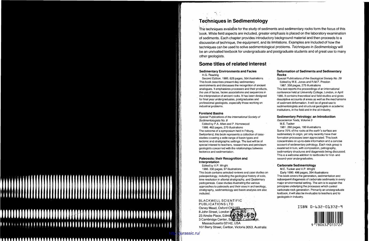
Techniques in Sedimentology Thes techniques available for the study of sediments and sedimentary rocks form the focus of this book. While field aspects are included, greater emphasis is placed on the laboratory examination of sediments. Each chapter provides introductory background material and then proceeds to a discussion of technique, the equipment, and its limitations. Examples are included of how the techniques can be used to solve sedimentological problems. Techniques in Sedimentology will be an unrivalled textbook for undergraduate and postgraduate students and of great use to many other geologists.
Some titles of related interest Sedimentary Environments and F a c i e s
H.G. Reading Second Edition. 1986. 628 pages, 564 illustrations
This book describes present day sedimentary environments and discusses the recognition of ancient analogues. It emphasizes processes and their products, the useof facies, facies associations and sequences in the interpretation of ancient rocks. It has been designed for final year undergraduates, postgraduates and professional geologists, especially those working on industrial problems.
Foreland B a s i n s Special Publications of the International Society of Sedimentologists No. 8
Edited by P.A. Allen and P. Homewood 1986. 462 pages, 270 illustrations
The outcome of a symposium held in Friburg, Switzerland, this book represents a collection of case-studies covering a wide range of basin types and tectonic and stratigraphic settings. The text will be of special interest to teachers, researchers and petroleum geologists concerned with the relationships between tectonics and sedimentation.
P a l e o s o l s : their Recogni t ion and Interpretation
Edited by V.P.Wright 1986. 330 pages, 97 illustrations
This book contains selected reviews and case studies on paleopedology, including the geological history of soils, time resolution in alluvial stratigraphy, and Quaternary pedogenesis. Case studies illustrating the various approaches to paleosols and their uses in archaeology, stratigraphy, sedimentology and basin analysis are also included.
BLACKWELL SCIENTIFIC PUBLICATIONS LTD Osney Mead, Oxford 0> 8 John Street, London i 23 Ainslie Place, Edinb 3 Cambridge Center,
Massachusetts 02142, USA 107 Barry Street, Carlton, Victoria 3053, Australia
Deformation of S e d i m e n t s and Sedimentary R o c k s Special Publications of the Geological Society No. 29
Edited by M.E. Jones and R.M.F. Preston 1987. 358 pages, 275 illustrations
This text reports the proceedings of an international conference held at University College, London, in April 1985. It contains theoretical and field studies and gives descriptive accounts of areas as well as the mechanisms of sediment deformation. It will be of great use to sedimentologists and structural geologists in academic institutions, in the field and in the oil industry.
Sedimentary Petrology: an Introduction Geoscience Texts, Volume 3
M.E.Tucker 1981. 260 pages, 180 illustrations
Some 70% of the rocks at the earth's surface are sedimentary in origin, yet only recently have their formation processes been appreciated. This book concentrates on up-to-date information and a concise account of sedimentary petrology. Each rock group is examined in turn, with composition, petrography, sedimentary structures and diagenesis being discussed. This is a welcome addition to textbooks for first- and second-year undergraduates.
Carbonate S e d i m e n t o l o g y M.E. Tucker and V.P. Wright Early 1990. 496 pages, 394 illustrations
This book covers the generation, sedimentation and subsequent diagenesis of carbonate sediments in every major environmental setting. The aim is to explain the principles underlying the processes which control carbonate rock generation. Primarily an undergraduate textbook, it will also be invaluable to teachers and to geologists in industry.
I S B N 0 - b 3 E - D 1 3 7 5 - T
9 l l 7 8 0 6 3 2 " 0 1 3 7 2 2 n
http://jurassic.ru/
Related Documents