Techniques for Interfacing Electromagnetic Transient Simulation Programs With General Mathematical Tools IEEE Taskforce on Interfacing Techniques for Simulation Tools

2610 IEEE TRANSACTIONS ON POWER DELIVERY, VOL. 23, NO. 4, OCTOBER 2008

Techniques for InterfacingElectromagnetic Transient Simulation

Programs With General Mathematical ToolsIEEE Taskforce on Interfacing Techniques for Simulation Tools

S. Filizadeh, Member, IEEE, M. Heidari, Student Member, IEEE, A. Mehrizi-Sani, Student Member, IEEE,J. Jatskevich, Senior Member, IEEE, and Juan A. Martinez, Member, IEEE

Abstract—This paper describes methods and issues related to in-terfacing electromagnetic transient simulation programs with gen-eral mathematical algorithms, which are either custom-developedby the user or are available through other mathematical analysisplatforms. Various interfacing types and techniques are describedalong with potential areas of application. Implementation methodsare detailed for each type of interface as well. This paper presentsseveral interfacing examples from a wide variety of applications,including advanced switching schemes for power converters andcontroller implementation.

Index Terms—Electromagnetic transient simulation, inter-facing, mathematical algorithms.

I. INTRODUCTION

I NTERCONNECTED electric power networks are large dy-namical systems with complex interactions. The analysis

and design of these systems often requires use of an array ofsimulation tools that represent the system behavior in a mannersuitable for the intended studies. Simulation tools enable theuser (e.g., system operator or designer) to assess various aspectsof the operation of the network with ease and without recourseto repetitive prototyping, or costly and potentially harmful testson the real system.

The level of detail used in the modeling of individual ele-ments and the choice of the solution method used in a simula-tion tool depend on the nature of the phenomena and require-

Manuscript received December 28, 2007. First published May 7, 2008; cur-rent version published September 24, 2008. Paper no. TPWRD-00811-2007

S. Filizadeh and M. Heidari are with the Department of Electrical and Com-puter Engineering, University of Manitoba, Winnipeg, MB R3T 5V6, Canada(e-mail: [email protected]; [email protected]).

A. Mehrizi-Sani is with the Department of Electrical and Computer Engi-neering, University of Toronto, Toronto, ON M5S 3G4, Canada (e-mail: [email protected]).

J. Jatskevich is with the Department of Electrical and Computer Engineering,University of British Columbia, Vancouver, BC V6T 1Z4, Canada (e-mail:[email protected]).

J. A. Martinez is with the Department d’Enginyeria El̀ctrica of the UniversitatPolitècnica de Catalunya, Catalunya 080208, Spain (e-mail: [email protected]).

Task Force on Interfacing Techniques for Simulation Tools is with theWorking Group on Modeling and Analysis of System Transients Using DigitalPrograms, IEEE Power Engineering Society T&D Committee.

Task Force members: U. Annakkage, V. Dinavahi, S. Filizadeh, A. M. Gole,R. Iravani, J. Jatskevich, A. J. Keri, P. Lehn, J. A. Martinez, B. A. Mork, A.Monti, L. Naredo, T. Noda, A. Ramirez, M. Rioual, M. Steurer, K. Strunz.

Digital Object Identifier 10.1109/TPWRD.2008.923533

ments of the studies to be carried out. While simplified modelssuffice in studies such as load flow, detailed, frequency-depen-dent models of individual elements, including nonlinear andswitching components, need to be used when short-term, high-frequency events are concerned [1].

As the complexity of power systems grows, the need formore sophisticated simulation tools escalates. Modern sim-ulation programs have been adapted to this increasing needby such measures as: 1) incorporation of improved user in-terfaces [2]; 2) enhanced analysis tools [3]; and 3) pre andpostprocessing mechanisms [4], [5]. There has, however, beena strong tendency to interface existing simulation tools to obtainfurther-enhanced simulation capabilities. This approach canideally allow for a synergetic combination of simulation tools.

Interfacing allows the constituent components (i.e., the sim-ulation tool and the external algorithms/tools) to communicatein a specified manner in order to carry out the overall simula-tion cooperatively and efficiently. The level of cooperation be-tween the interfaced tools can range from mere postprocessingand visualization of simulation results [4] to relegating an in-tegral part of the simulation to an external tool where specificanalyses can be done more effectively than in the original sim-ulation tool [6]–[8].

This paper addresses aspects related to interfacing elec-tromagnetic transient simulation tools [ElectromagneticTransients Program (EMTP)-type programs] with other mathe-matical tools, including both external programs and stand-alonealgorithms. Interfacing EMTP-type tools with external pro-grams/algorithms extends their applicability in areas wheremore streamlined techniques (e.g., for sophisticated controlsystem design, are available through the external agent). Shorterdevelopment time and increased credibility of results are otherexamples of the benefits of interfacing an EMTP-type tool witha tested and verified external algorithm.

Various kinds of interfaces and methods for their implemen-tation are presented in the paper. For illustration purposes, thePSCAD/EMTDC electromagnetic transient simulation programis used; however, the methods are treated in a generic manner toensure they remain applicable to arbitrary EMTP-type tools.

II. ELECTROMAGNETIC TRANSIENT SIMULATION TOOLS

Electromagnetic transient simulation tools are used to studyshort-term behavior of complex electrical systems. Due to the

0885-8977/$25.00 © 2008 IEEE

Authorized licensed use limited to: The University of Toronto. Downloaded on October 10, 2009 at 23:49 from IEEE Xplore. Restrictions apply.

FILIZADEH et al.: TECHNIQUES FOR INTERFACING ELECTROMAGNETIC TRANSIENT SIMULATION PROGRAMS 2611

Fig. 1. Schematic diagram of a generic EMTP-type tool.

high level of detail used in representation of system elements,computational intensity of these programs (e.g., CPU require-ments), is typically high and their use is mostly limited to net-works smaller than what is possible in stability analysis pro-grams [1], [9].

These tools have been used extensively for the analysis anddesign of various elements of modern systems, where transients(often fast transients) are involved. Typical applications includedesign of controllers for power apparatus [10], overvoltage andinsulation coordination [11], [12], protection [13], flexible actransmission systems (FACTS) [14], HVDC [15], [16], andother power-electronic applications [17].

The majority of commercially available EMTP-type pro-grams use nodal analysis (admittance matrix formulation) andnumerical integration to setup and solve system equationsin a progressive manner and in time domain [18], [19]. Thisformulation is based on the pioneering work by H. W. Dommelin 1969 [1]. Other formulation methods such as state spacemethod have also been used [20], but their mechanics are notdiscussed here.

Fig. 1 shows a schematic diagram of a generic electromag-netic transient simulation program. Aside from minor modifica-tions introduced by add-on features such as interpolation [21],the overall method for solution of system equations is based ona discretized time axis, where the entire simulation time isdivided into small intervals, each with a constant width of ,which is referred to as the simulation time step. Use of a fixedtime step allows for simplified modeling and expedites the sim-ulation by eliminating the need for inverting the network admit-tance matrix repetitively.

The solver of the system equations in each time step usescharacteristics of the electrical elements and also those of dy-namical devices, such as machines and controls, to obtain up-dated node voltages. Solution in each time step in general re-quires some information from previous time step(s). Such his-tory terms are encountered both in electrical network elements(e.g., capacitors and inductors), and in control functions such asintegrators [1], [22], [23].

III. NEED FOR INTERFACING

Commercially available transient simulation tools include afairly comprehensive library of components that allow the userto conveniently assemble a circuit for the purpose of simula-tion. These so-called library components may represent sources,electric machines, cables and transmission lines, semiconductorand power electronic devices, and control and processing func-tions (e.g., gain blocks, PI controllers, and integrators).

Despite the availability of standard library components, usersoften find that components for performing specialized compu-tations are not readily available. Therefore, there is a need toextend the capabilities of these programs by incorporating fa-cilities for performing such computations. In EMTP-type pro-grams, these facilities are provided through enabling user-de-fined components and/or interfacing to other simulation soft-ware or programming languages [19], [24].

Interfacing has been used for simulation of complex pro-tection systems [25], development of advanced digital controlsystems [26], and simulation of power electronic convertersusing EMTP-TACS [3]. An interface that uses synchronizingclocks for connecting a simulation program with a real con-troller hardware is proposed in [27]. Attempts have alsobeen made towards development of simulation platforms inwhich multiple tools interact. Examples of interfaces betweenPSCAD/EMTDC and MATLAB/SIMULINK are presented in[4], [28], and [29]. A different interfacing method in whichan entire simulation is broken into smaller pieces is reportedin [30] and is demonstrated using the CIGRE HVDC bench-mark model [31]. In [32], a transient simulator is interfacedwith a nonlinear simplex optimization algorithm written inFORTRAN to add optimization features to the simulator. Acomprehensive example of interfacing between a transient sim-ulator and MATLAB/SIMULINK and a comparison betweenEMTDC and MATLAB/SIMULINK-PSB is presented in [33],in which CIGRE HVDC benchmark model [31] is consideredas the base network.

Besides EMTP-type tools, interfacing has also been used forinterconnecting electronic circuit simulators as well. Reference[34] presents DELIGHT.SPICE, which is an integration of DE-LIGHT interactive optimization-based CAD system and SPICEfor circuit optimization. Reference [35] interfaces optimizationroutines written in MATLAB with SABER circuit simulator.References [36] and [37] show other examples of interfacingcircuit simulation programs with optimization algorithms.

IV. METHODS FOR INTERFACING

The method used for interfacing EMTP-type tools with otheralgorithms and the level of complexity involved in doing so de-pend on the problem it targets to solve. In the following subsec-tions, a number of interfacing methods will be addressed.

A. Static Interfacing

Consider for example interfacing a transient simulator withan external agent in order to plot traces of simulated variables.Ordinarily, one needs to establish a channel between the simu-lator and the plotting agent to send (in a unidirectional manner)data for the intended variables as they are obtained at each timestep. Note that no buffer is necessary to store past values, as datais sent to the plotting agent as it becomes available. Moreover,



Fig. 2. Static interface to an external algorithm.

one may note that plotting every point on the simulated traceis not necessary and plotting the waveform sampled at regularintervals (other than every time step) still produces graphs ofacceptable accuracy. Therefore, it is possible to lower the com-munication burden by calling the plotting algorithm at regularintervals with a width of samples. The time line shown inFig. 2 depicts the procedure graphically for intermittent com-munication with an external algorithm. Static interfacing maybe used for such purposes as plotting or computation of com-plex functions.

When the simulation case is assembled, the code sections per-taining to the components used are gathered along with theircontrol law. Thus, at every time step, the code for each compo-nent is run only if its control law so allows.

Static interfaces have been further categorized as online oroffline [4]. In an online interface, the transient simulation toolcommunicates with the external algorithm throughout the sim-ulation (e.g., in the visualization example later in this paper). Inan offline interface, an external tool is called following the com-pletion of the simulation, which does further processing on thesimulated data.

B. Dynamic Interfacing and Memory Management

Dynamic interfaces are more involved than static ones, asmemory management becomes an integral part of the interface.Processes that simulate dynamic elements, such as controllersor filters, fall in this category. Unlike static interfaces, in whichonly data from the current time step are communicated betweenthe transient simulator and the interfaced algorithm, dynamicinterfaces exchange current as well as past data.

As an example of a dynamic interface, consider a peak-de-tection component. The component is supposed to track a givensignal and find its peak value and update its output when-ever a higher peak is detected. The peak-detector algorithm willbe shown.

The algorithm uses a storage variable to storethe last peak detected. Although the algorithm is quite simple,its implementation requires access to memory location(s) thatare kept intact from one time step to the next. These memorysegments are used for storing variables by components that needsuch storage, and transient simulation tools often provide accessto this kind of storage.

An important issue when dealing with memory segments isto note that the pointers to memory locations should be updatedand maintained in a unified manner. Since in each time step,the simulation executes the code of individual elements in theorder they are placed within the code, it is important to ensurethat the stored variables can be retrieved properly. By properly

incrementing the pointers, it is guaranteed that they always pointto the correct memory locations for all components.

ALGORITHM 1—PEAK DETECTION

1 if current simulation time ��

2 ��

3 ��

4 Else

5 if ��

6 ��

7 End

8 ��

9 End

C. Wrapper Interfaces

A wrapper interface is one that does not communicate withthe transient simulator on a regular basis throughout the simula-tion as static and dynamic interfaces do. Instead, it has limitedcommunication at specific points in time, normally at the be-ginning and end of a simulation. This kind of interface is madewhen external code controls the simulations in a certain way.An example of this interface is given in Section VII, where op-timization and run-control algorithms are discussed.

Note that a wrapper interface is different from an off-line onein that the wrapper interface is often a supervisory algorithm thatcontrols the simulation program and normally performs mul-tiple simulations, whereas an offline interface is usually meantto perform postprocessing of simulation results.

V. WHERE TO IMPLEMENT: EXTERNAL

VERSUS INTERNAL INTERFACES

Once an algorithm is developed or selected for interfacingwith a simulation tool, one needs to decide where to implementthe algorithm. Options for implementation will be discussed.

A. External Interfaces

For algorithms that are available externally through stand-alone software, external interfacing is normally the most logicaloption. Depending on the input/output configuration of the al-gorithm, external interfacing can potentially eliminate the needfor rewriting the external code in the indigenous language ofthe simulation tool. Physical establishment of the interface re-quires access to the memory management routines of the tran-sient simulator. An example of an external interface is inter-facing an EMTP-type program to MATLAB [24], which al-lows the user to store required variables in predefined locations,called MATLAB, to execute a standard or user-developed code,and retrieve data back to the simulation program for further pro-cessing. The interface may allow execution of the external al-gorithm in each time step or intermittently; therefore, both dy-namic and static interfaces described earlier can be implementedexternally.

An important observation about external interfacing is thespeed implications involved. Transient simulation tools oftenuse optimized methods for enhancing simulation speed. Ex-ternal programs, however, are not necessarily designed with



such provisions. Therefore, a simulation tool that uses aninterface with an external program can be drastically slowerthan the same procedure implemented entirely internally in theEMTP-type tool. Apart from the intrinsic speed differences be-tween the two agents, the overhead of communication betweenthe programs can also significantly affect the overall simulationperformance. Unless they are high speed, efficient communi-cation methods are deployed, exchange of large amounts ofdata between the interfaced tools normally results in a markedreduction in the speed. The problem will be exacerbated if theinterface is used as part of a multirun simulation.

Depending on the facilities present in the externally inter-faced tool, this type of interfacing can serve as a powerful meansfor rapid algorithm development, verification, and debugging. Itis sometimes easier to make changes to an algorithm developedin a dedicated external agent such as MATLAB than one imple-mented in the rigidity of an EMTP-type program. Modificationscan be easily done and tested through the combined interface.If the speed reduction due to external interfacing is severe, onecan consider converting the external interface to an internal one.

Another important aspect of external interfacing is the abilityof interfacing to multiple platforms. For example, when anEMTP-type tool is interfaced with MATLAB, other simulationtools (e.g., SIMULINK) or mathematical and programmingtools (e.g., coding in multiple languages) may become availableas well.

B. Internal Interfaces

A method to alleviate drawbacks associated with externalinterfaces is to use internal interfacing, where a user-suppliedalgorithm (unavailable in the transient simulation tool) is im-plemented within the transient simulator. Internal interfacing ispossible when the user has access to the code of the algorithmand is knowledgeable about its inner workings.

Internal interfaces have been used for interfacing nonlinearoptimization algorithms with transient simulators (describedlater). Dynamical models of electric vehicles [38], advancedswitching schemes for power converters [39], and specializedmotor drives and mechanical models for vehicular powersystems [38], [40] have also been interfaced using internalinterfacing mechanisms.

Note that internal interfaces are faster than external ones dueto the elimination of the communication overhead. However,their implementation is normally more involved than externalones.

VI. MULTIPLE INTERFACING

In addition to the main high-power electric circuitry, modernpower equipment often contains advanced control blocks, dig-ital processors, nonlinear elements, etc. Proper simulation ofthese systems should allow uncompromised analysis, and assuch, it is sometimes necessary to interface more than two sim-ulation programs, each with special features for detailed mod-eling of certain aspects of a complex circuit. In this section,some of the schemes for multiple interfacing of a transient sim-ulation programs with other simulation programs or mathemat-ical tools are explained. Variations of these schemes are obvi-ously possible, but are not discussed here.

Fig. 3. Core-type interfacing.

Fig. 4. Variations of chain-type interfacing. (a) Chain-type interfacing for preand postprocessing. (b) Chain-type interfacing for linking noncompatible sim-ulators.

A. Core-Type Interfacing

In core-type interfacing of simulation programs, one programserves as the core and all of the other (auxiliary) programs areconnected to the core. Fig. 3 shows a block diagram of such astructure. The auxiliary programs in this structure can be im-plemented externally or internally (refer to Section V), and maymanifest static, dynamic, or wrapper properties as discussed ear-lier.

The core-type interfacing structure usually occurs when amajor portion of the system under study can be modeled in asingle simulation program (the core), and the auxiliary programsare assigned minor tasks, such as data visualization or other cal-culations. The firing pulse generation and visualization exampleshown later in this paper is a core-type interface, in which gen-eration of firing pulses and visualization tasks are assigned toauxiliary algorithms that communicate with the core simulatorin which the main power circuit is simulated.

B. Chain-Type Interfacing

Unlike a core-type interface where the core program is usedas a common node for all other programs, in chain-type inter-facing, the simulation programs are connected to each other ina row. There are two common templates for chain-type inter-facing, as shown in Fig. 4.

In the first scheme [see Fig. 4(a)], chain-type interfacing isused for preprocessing and postprocessing of the data. As anexample, consider simulation of a network with transmissionlines. Prior to simulating the network, an algorithm is often usedto calculate the line constants to be used in the actual simu-lator (preprocessing); visualization of the simulated data usinga graphing program constitutes postprocessing and the entirescheme takes on the form of a chain-type interface.



Fig. 5. Loop interfacing scheme.

A second variation of a chain-type interface [see Fig. 4(b)]may be used when simulation programs cannot be interfaceddirectly and readily. An intermediate agent, such as MATLAB,can be used to bridge the interfacing gap between originallyincompatible simulators.

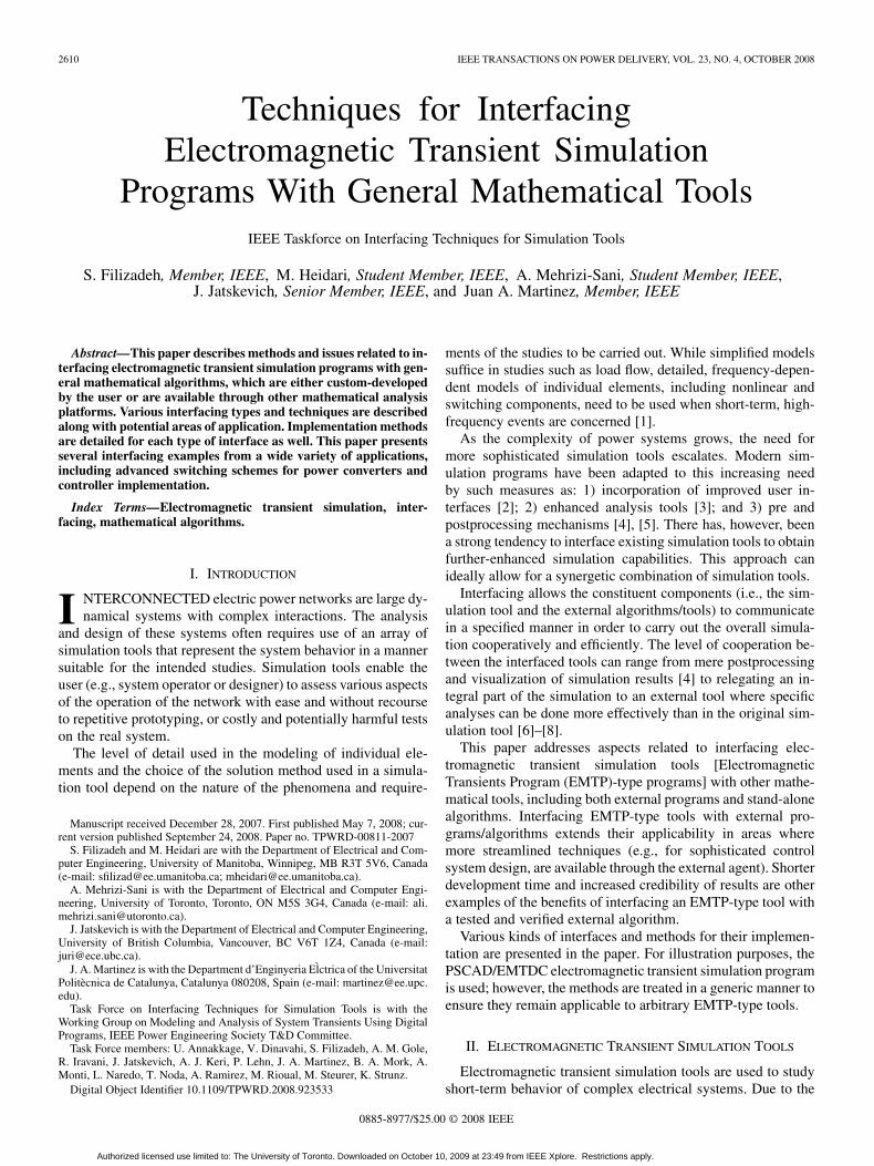
C. Loop Interfacing

If in a chain of simulation programs or external hardware, thelast program is also connected to the first one, the result will bea loop interfacing scheme, as shown in Fig. 5. Such combina-tions occur frequently when real-time simulators are connectedto several interacting external pieces of equipment (e.g., relays,controllers, amplifiers, and digital signal processors [41]). Sinceinterfacing of real-time simulators is not the focus of this paper,loop interfacing is not discussed in any further detail.

VII. EXAMPLES OF INTERFACING

A. Interfacing to MATLAB/SIMULINK

This section explains an interface made between a transientsimulator (PSCAD/EMTDC) and MATLAB/SIMULINK.Similar interfaces have also been made between EMTP andMATLAB [24]. These interfaces can be used in a variety ofways, allowing full exploitation of the computational facilitiesin MATLAB and modeling capabilities of SIMULNK.

The interface between the EMTP-type simulation engine andMATLAB is essentially an external interface. The transient sim-ulation engine can communicate with MATLAB either in eachtime step or intermittently, depending on the nature and require-ments of the externally sourced task.

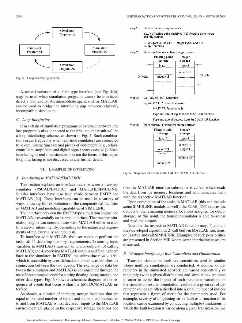
To interface with MATLAB, the user needs to perform thetasks of: 1) declaring memory requirements; 2) storing inputvariables to MATLAB (transient simulator outputs); 3) callingMATLAB; and 4) receiving MATLAB outputs and feeding themback to the simulator. In EMTDC, the subroutine MLAB_INT,which is accessible by user-defined components, establishes theconnection between the two agents. The exchange of data be-tween the simulator and MATLAB is administered through theuse of data storage queues for storing floating-point, integer, andother data types. Fig. 6 shows a schematic diagram of the se-quence of events that occur within the EMTDC/MATLAB in-terface.

As shown, a number of memory storage locations that areequal to the total number of inputs and outputs communicatedto and from MATLAB is first declared. Inputs to the MATLABenvironment are placed in the respective storage locations and

Fig. 6. Sequence of events in the EMTDC/MATLAB interface.

then the MATLAB interface subroutine is called, which readsthe data from the memory locations and communicates themwith the respective MATLAB function.

Upon completion of the tasks in MATLAB (this can includesome SIMULINK models as well), the MLAB_INT returns theoutputs to the remaining memory locations assigned for outputstorage. At this point, the transient simulator is able to accessand read the outputs.

Note that the respective MATLAB function may: 1) containuser-developed algorithms, 2) call built-in MATLAB functions,or 3) setup and call SIMULINK. Examples of such possibilitiesare presented in Section VIII where some interfacing cases arediscussed.

B. Wrapper Interfacing: Run Controllers and Optimization

Transient simulation tools are sometimes used in studieswhere multiple simulations are conducted. A number of pa-rameters in the simulated network are varied sequentially orrandomly (with a given distribution) and simulations are donein order to assess the impact of such parameter variations onthe simulation results. Simulation results for a given set of pa-rameter values are often distilled into a small number of indicesthat represent a figure of merit for the parameters used. Forexample, severity of a lightning-strike fault as a function of itslocation can be examined by conducting multiple simulations inwhich the fault location is varied along a given transmission line



Fig. 7. Optimization interfacing.

and the magnitude of the resulting voltage surge is recorded.EMTP-type tools often provide built-in engines for conductingmultiple simulations using specified parameter variations [19].

The so-called multiple-run simulation can be describedas in the following algorithm (Algorithm 2). As shown, themultiple-run algorithm is responsible for: 1) selecting suitableparameter values according to the specified parameter variationrule, 2) feeding the simulation with the parameters, and 3)recording the respective figure of merit for further processing.

ALGORITHM 2—MULTIPLE-RUN SIMULATIONS

1 create a set of parameters Pi (a total of Npoints representing parameter combinations)

2 � � �

3 if � ��

4 run the simulator with parameter set P(i)

5 record the figure-of-merit for P(i)

6 � � � � �

7 End

Note that the preselection of parameter combinations in a se-quential multiple-run, or random selection with a given distri-bution resembles a passive approach to the true potential of themultiple-run algorithm. Through proper interfacing, however,one can design more advanced run-control algorithms to con-duct multiple simulations in ways other than the conventionalapproach, where it is possible to steer future simulations basedon the outcome of current and past simulations.

1) Interfacing to an Optimization Algorithm: An exampleof an enhanced multiple-run algorithm without a predeterminedset of search parameters is the optimization facility in a transientsimulation program. Some EMTP-type programs have incorpo-rated nonlinear optimization as an integral part of the simulationsuite [19], [42]. Here, a nonlinear optimization algorithm canbe called to replace the conventional multiple-run algorithm toconduct several simulations, each with a new set of parametersdetermined by the optimization algorithm according to the col-lective history of past simulations [32]. Fig. 7 shows a schematicdiagram of the simulator–optimization interface.

Note that unlike a conventional multiple-run simulation, thenonlinear optimization algorithm decides, based on the objec-tive function value it receives from the simulation program and

Fig. 8. Excerpt of a generic optimization algorithm.

the history of past simulations, what parameter values need tobe generated and submitted to the simulation program for thenext simulation.

An optimization engine implemented in ETMDC is inter-faced internally and is used to link a number of optimizationalgorithms to the simulation engine, including nonlinear sim-plex of Nelder and Mead [43], genetic algorithms, and a numberof gradient-based algorithms [44]. The choice of an internalinterface has been made to remove potential speed reductionsand to expedite the design cycle that normally involves severalsimulations. There are, however, advanced optimization algo-rithms that make use of complex functions that are available inmathematical software such as MATLAB, and their implemen-tation is either excessively complicated or not possible due to theconfidentiality of the code. For such cases, external interfacingbetween the simulation program and MATLAB has been used[45]. In this case, the interface resembles a master/slave relation-ship, where the host of the optimization algorithm (MATLAB)also serves as the master and calls upon the slave (transient sim-ulation tool) for objective function evaluation.

Internal interfacing of optimization algorithms, however, em-beds some challenges that need detailed knowledge of the me-chanics of the simulation tool. Consider optimization of thefunction , whose evaluation is done through simulation(refer to Fig. 7 for details). A heuristic optimization algorithmoften compares objective function evaluations at a number ofpoints within the algorithm in order to generate new parametervalues. Therefore, a portion of such an optimization algorithmmay be as shown in Fig. 8.

After initializing two sets of parameter values ( andin line 1), the algorithm needs to compare their correspondingobjective functions (line 2). However, each of the two values

and are obtained by transient simulation ofthe network using the simulation tool itself, which requirestwo complete simulations. In other words, the optimization,embedded within and called by the simulation tool, will callthe simulation tool at several locations, thus creating a nestedloop. Appropriate use of flags and control statements ensuresthat sequence of the execution of statements in the simulationprogram is transferred to the exact location where it was inter-rupted.

2) Advanced Run Controllers: Aside from optimization,there are other types of multiple-run controllers that use theconcept of adaptive steering of simulations. An example ofthis is reported in [46] where an adaptive, internally interfacedsearch algorithm is used for finding the largest value of aninductor and its critical point-on-wave switching instant thatresult in no commutation failure at the terminals of an HVDCconverter.



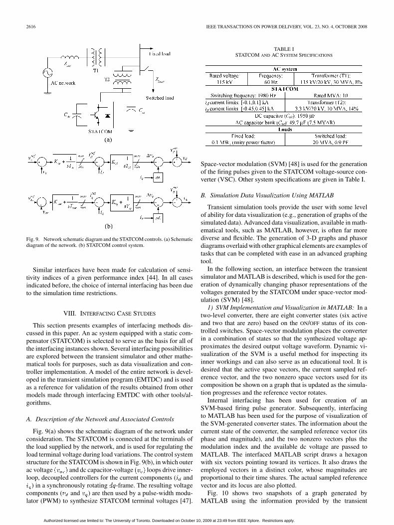
Fig. 9. Network schematic diagram and the STATCOM controls. (a) Schematicdiagram of the network. (b) STATCOM control system.

Similar interfaces have been made for calculation of sensi-tivity indices of a given performance index [44]. In all casesindicated before, the choice of internal interfacing has been dueto the simulation time restrictions.

VIII. INTERFACING CASE STUDIES

This section presents examples of interfacing methods dis-cussed in this paper. An ac system equipped with a static com-pensator (STATCOM) is selected to serve as the basis for all ofthe interfacing instances shown. Several interfacing possibilitiesare explored between the transient simulator and other mathe-matical tools for purposes, such as data visualization and con-troller implementation. A model of the entire network is devel-oped in the transient simulation program (EMTDC) and is usedas a reference for validation of the results obtained from othermodels made through interfacing EMTDC with other tools/al-gorithms.

A. Description of the Network and Associated Controls

Fig. 9(a) shows the schematic diagram of the network underconsideration. The STATCOM is connected at the terminals ofthe load supplied by the network, and is used for regulating theload terminal voltage during load variations. The control systemstructure for the STATCOM is shown in Fig. 9(b), in which outerac voltage and dc capacitor-voltage loops drive inner-loop, decoupled controllers for the current components ( and

) in a synchronously rotating -frame. The resulting voltagecomponents ( and ) are then used by a pulse-width modu-lator (PWM) to synthesize STATCOM terminal voltages [47].

TABLE ISTATCOM AND AC SYSTEM SPECIFICATIONS

Space-vector modulation (SVM) [48] is used for the generationof the firing pulses given to the STATCOM voltage-source con-verter (VSC). Other system specifications are given in Table I.

B. Simulation Data Visualization Using MATLAB

Transient simulation tools provide the user with some levelof ability for data visualization (e.g., generation of graphs of thesimulated data). Advanced data visualization, available in math-ematical tools, such as MATLAB, however, is often far morediverse and flexible. The generation of 3-D graphs and phasordiagrams overlaid with other graphical elements are examples oftasks that can be completed with ease in an advanced graphingtool.

In the following section, an interface between the transientsimulator and MATLAB is described, which is used for the gen-eration of dynamically changing phasor representations of thevoltages generated by the STATCOM under space-vector mod-ulation (SVM) [48].

1) SVM Implementation and Visualization in MATLAB: In atwo-level converter, there are eight converter states (six activeand two that are zero) based on the ON/OFF status of its con-trolled switches. Space-vector modulation places the converterin a combination of states so that the synthesized voltage ap-proximates the desired output voltage waveform. Dynamic vi-sualization of the SVM is a useful method for inspecting itsinner workings and can also serve as an educational tool. It isdesired that the active space vectors, the current sampled ref-erence vector, and the two nonzero space vectors used for itscomposition be shown on a graph that is updated as the simula-tion progresses and the reference vector rotates.

Internal interfacing has been used for creation of anSVM-based firing pulse generator. Subsequently, interfacingto MATLAB has been used for the purpose of visualization ofthe SVM-generated converter states. The information about thecurrent state of the converter, the sampled reference vector (itsphase and magnitude), and the two nonzero vectors plus themodulation index and the available dc voltage are passed toMATLAB. The interfaced MATLAB script draws a hexagonwith six vectors pointing toward its vertices. It also draws theemployed vectors in a distinct color, whose magnitudes areproportional to their time shares. The actual sampled referencevector and its locus are also plotted.

Fig. 10 shows two snapshots of a graph generated byMATLAB using the information provided by the transient



Fig. 10. Snapshots of the SVM visualization output in MATLAB.

simulator. At the given instants of time, the reference vectorsand their projections onto respective space vectors are shown.

2) Interfacing Aspects: Since this type of interfacing onlytransmits data from the main simulator (EMTP-type program) tothe visualization platform (MATLAB) and does not involve anystorage or manipulation of the data, it is categorized as a static,external, core-type interface. Moreover, the data are transmitted(intermittently) throughout the simulation, making it an onlineinterface.

C. Modeling of Control Systems in MATLAB/SIMULINK

In this section, the use of (external) interfacing for modelingof control systems in MATLAB/SIMULINK is demonstrated.The intention is to highlight the interfacing aspects and assuch, two simple scenarios are considered for implementationof the STATCOM control system shown in Fig. 9(b): 1) mod-eling entirely in MATLAB, and 2) modeling in MATLAB andSIMULINK. The control system is then interfaced with thepower circuits that are modeled in the main transient simulator.A separate model developed entirely in the transient simulatoris used as the basis for validation.

1) PI Controller Implementation in MATLAB: Control algo-rithms can be directly coded in MATLAB and called for gener-ation of controller output(s). Consider, for example, the imple-mentation of the ac voltage controller (proportional gain ,integral time constant ) in Fig. 9(b). Its implementation inMATLAB involves the development of the integrator and pro-portional actions and imposing the limits (as given in Table I).Limits similar to those used for the entire PI block are also im-posed on the integrator. This ensures that the integrator does notplunge deeply into saturation, and expedites the response timeof the PI controller. The integrator action is implemented usingtrapezoidal integration method. A component is developed thataccepts the ac voltage magnitude error (as its input) and commu-nicates it along with the current simulation time and time stepwith a MATLAB function that implements the PI action.

Similar to the procedure outlined in Fig. 6, the interface com-ponent stores the input variables in the respective queue, calledthe MLAB_INT subroutine, which, in turn, runs the MATLABfunction for the PI action, and retrieves the PI controller outputfrom the respective memory location. Fig. 13 shows traces ofthe ac voltage variations when the network is subjected to a loaddisconnection at 0.4 s followed by its reconnection at 0.6 s. Thetraces are shown for both the standard PI controller block of theEMTDC as well as the PI controller implemented in MATLABand interfaced with the transient simulator. As expected, thewaveforms are identical and overlap.

Fig. 11. Sequence of events in the SIMULINK interface.

Fig. 12. SIMULINK model of the ac voltage PI controller.

2) Control System Implementation in MATLAB/SIMULINK:As the complexity of systems to be modeled in MATLAB (orother external agents) increases, it becomes increasingly dif-ficult to write detailed codes for calculations or controller ac-tions as was done in the previous example. Use of SIMULINK,which offers a graphical interface for development of complexinterconnected systems, can highly simplify this task. An im-plementation of the PI controller in the previous section is thusundertaken using the SIMULINK.

For this purpose, an interface to MATLAB is developed,which in turn sets the simulation and workspace parametersfor a SIMULINK model of the PI controller and invokesSIMULINK for the actual simulation. Communication of theinputs and outputs to and from MATLAB follows the sequencedepicted in Fig. 6. The sequence of events in the SIMULINKinterface is shown in Fig. 11. Note that the SIMULINK modelis executed only for the interval each time it isinvoked. Fig. 12 shows the developed SIMULINK model of theac voltage PI controller.

The latest state of the integrator needs to be saved at the endof the interval, so that it can be used as the initialstate for the next time step; therefore, an external input is addedto the integrator block (input port 2 in Fig. 12) so that the correctinitial state can be fed into the integrator. Similar to the originalPI controller in EMTDC and the one coded in MATLAB in thepreceding section, identical lower and upper limits ( 0.45 and0.45, respectively) are applied to both the integrator and the en-tire PI block outputs. The SIMULINK model shown in Fig. 12has been interfaced with the transient simulation model of theSTATCOM system and has been tested for the same set of distur-bances described in the previous section. Fig. 13 shows the sim-ulation results obtained, which are identical to the ones depictedfor the original model and the MATLAB-interfaced model (bothmodels start from zero initial conditions).

3) Computer Time and Interfacing: As indicated earlier, ex-ternally interfaced tools tend to be slower than their internal



Fig. 13. Simulated waveforms for various network modeling approaches. (a)Capacitor voltage waveform. (b) Load terminal voltage waveform.

TABLE IICOMPARISON OF SIMULATION TIME FOR THE STATCOM CASE

counterparts. An audit of the simulation time often reveals im-portant information about the intensity of interfacing. Table IIshows computer times used for the simulation of the STATCOMsystem in the EMTDC, EMTDC interfaced with MATLAB andEMTDC interfaced with SIMULINK. The simulation time in-terval is 0.8 s and is traversed using a 5 s time step and 100

s plot step on a Pentium 4, 3.0 GHz machine with 1.0 GB ofRAM.

The interfaced models in MATLAB and MATLAB/SIMULINK are slower than the original transient simula-tion model, as evidenced by their respective computer timesof 1258.3 s and 3531.5 s as opposed to 32.3 s in the EMTDC.This shows simulation times in excess of 1.5 and 2.0 ordersof magnitude slower than the original model, respectively. Itis therefore advisable that interfacing be used only when suchprolonged simulations times are offset by the benefits of thetool to which the interface is established.

D. Optimization and Sensitivity Analysis

1) Wrapper Interfacing for Gradient-Based Optimization:An optimization algorithm adopts an iterative approach to findthe optimum point of a function. By defining a suitable objec-tive function and use of an optimization algorithm to control thesimulation runs, it is possible to adjust the design parameters ofa circuit so that a given set of design objectives is met as closelyas possible.

Fig. 14. Simulation-based Fletcher–Reeves optimization tool.

This section considers a gradient-based technique known asthe Fletcher–Reeves method [49], and uses it for optimizationof the control system parameters of the STATCOM in Fig. 9(b).

The block diagram shown in Fig. 14 summarizes thesteps involved in the simulation-based optimization using theFletcher–Reeves method. As shown, the optimization algorithminteracts with the simulator in two stages. The first stage isdevoted to the calculation of partial derivatives, during whichincremental changes are made successively to the parametervalues, and the corresponding objective function values arecalculated by running the simulation program. For an -vari-able optimization problem, this stage requires simulations.During the second stage, the simulation program is run a fewtimes until a suitable step length (one which results in a re-duction in the value of the objective function) is obtained. Thealgorithm has been implemented in FORTRAN, and is usedas a wrapper interface (internally developed) to the transientsimulation program.

The optimization tool is used to obtain optimal values forthe parameters of the control system shown in Fig. 9(b). Thegoal of the optimization is to obtain smooth transitions in thenetwork voltage and the dc capacitor voltage when the networkis subjected to a load rejection/reconnection disturbance. Theobjective function used is as follows:

(1)

The objective function in (1) approaches zero as the networkvoltage and the dc capacitor voltage stay tightly close to theirreference values during transients and in steady state. Fig. 15shows the variations of the dc-capacitor voltage before and afteroptimization. The disturbances applied are a load rejection at 1.0s followed by its reconnection at 1.5 s. AC voltage variations areshown in Fig. 16. Both figures show significant improvement inthe performance of the system as a result of optimization.

The aforementioned optimization process takes about 300simulation runs to converge to an optimum point in about 5 h on



Fig. 15. DC capacitor voltage. (a) Before and (b) after optimization.

Fig. 16. Network voltage. (a) Before and (b) after optimization.

a 1.7 GHz Intel Celeron processor. Note that the number of sim-ulation runs required also depends on the optimization startingpoint (i.e., depending on how far the actual (local) optimum isfrom the starting point), the number of simulations required willchange accordingly.

2) Internal Wrapper Interface for Sensitivity Analysis: Dueto such factors as operating conditions and aging, circuit pa-rameters may deviate from their original values over time. Itis therefore important to evaluate the performance of a designwhen parameter values are subject to variations from their nom-inal values (i.e., to perform sensitivity analysis).

Interfacing an electromagnetic transient simulator with amathematical algorithm for sensitivity analysis can facilitatethe task by allowing (automatic) calculation of the partialderivatives of the desired performance index with respectto the design parameters . The partial derivatives can thenbe used to estimate the variations in the performance functionas follows:

(2)

Note that the calculation of the derivatives follows the mul-tiple–simulation approach outlined in Section VII; therefore, a

TABLE IIISENSITIVITY INDICES OF THE NETWORK USING SIMULATION

wrapper interface that feeds the simulator with proper param-eter values is developed that performs multiple simulations andcalculates the derivatives.

In the following, sensitivity analysis as described before isused to assess the impact of component aging and load vari-ations on the performance of the STATCOM control system.The settling time of the control system, defined as the timerequired for reaching and stabilizing in a band within 0.25%around the final steady-state operating point, is selected as theperformance index. Sensitivity of the settling time to varia-tions in the ac and dc capacitor sizes ( and ), STATCOMtransformer (T2) impedance , ac network impedance

, and load impedance is estimated using the de-veloped wrapper interface.

Since five design parameters are considered, estimation ofpartial derivatives using (2) requires ten simulations, each witha given parameter deviation (positive and negative incrementsare considered for calculation of derivatives). Table III showsthe estimated partial derivatives obtained using transient simu-lation of the network. As suggested by its large partial deriva-tive, variations in the ac capacitor bank have a significant im-pact on the settling time of the control system, in contrast to thelower impact expected from variations in the dc capacitor andload impedance.

One important study that can be performed using sensitivityindices is the worst-case scenario (i.e., to determine the largestpossible deviation in the performance index for given tolerancesin the design parameters). The worst-case (longest) settling timeof the STATCOM control system when the five selected systemparameters are allowed to vary within a given range (denoted by

in percent) can be obtained by using (3)

(3)

where is the worst-case settling time and is the orig-inal settling time for the original parameter settings. The settlingtime of the STATCOM control system for the original parame-ters values given in Table I is equal to 0.125 s, as evidencedby response of the load ac voltage shown in Fig. 17(a). For asmall tolerance of 2.5% in all five selected design parameters,the worst-case analysis using (5) with the numerically estimatedpartial derivatives in Table III, yields a settling time of 0.262 s.The actual simulation result obtained for the worst-case com-bination of the design parameters is shown in Fig. 17(b), andshows a settling time of 0.263 s, which agrees well with the es-timated worst-case value.



Fig. 17. AC voltage waveform for (a) the original system parameters, and (b)the worst-case combination of design parameters with 2.5% tolerance.

IX. OTHER INTERFACING OPPORTUNITIES

The majority of interfacing instances most likely fall withinone of the categories described previously in this paper. Thereare, however, other instances where interfacing becomes impor-tant. Two such cases are described below.

A. Interfacing With External Hardware

Transient simulation tools provide valuable informationabout short-term dynamics of a power system. For example,such detailed information becomes particularly useful whentuning and designing protection systems, which are required torespond in a timely fashion to faults and other maloperations ina network.

Although conventional transient simulation tools do not havesynchronized and real-time capabilities (except dedicated real-time simulators [50], [51]), their simulated waveforms can berecorded, and then played back in real time into external pro-tection hardware using amplifiers of appropriate bandwidth, andvoltage and current ratings in order to test the performance of theprotective relaying equipment in response to simulated faults.

Appropriate interfaces exist to enable recording and playingback of the simulated waveforms. Standard formats (e.g., COM-TRADE [52]), exist to facilitate communication between thesimulation tool and the external hardware. Note that playingback the simulated waveforms onto a protective relay can beused to investigate the behavior of the relay; however, since nodirect connection exists between the relay under test and thesimulator, the scheme does not form a closed-loop simulator inwhich simulation continues following the relay operation. Inter-facing techniques for hardware applications become more rel-evant with regards to real-time simulators; however, this fallsbeyond the scope of this paper.

B. Distributed Simulation and Co-Simulation

Transient simulation of large power networks requires mas-sive computer facilities. It is therefore beneficial if simulationscould be partitioned or performed on platforms comprising sev-eral processing units.

To take advantage of the distributed simulation, it is first nec-essary to partition the original network into two or more subsys-tems. The partitioning can happen, for example, at convenientboundaries involving natural delays such as transmission lines;more complicated systems with electrical networks, power elec-tronic converters, electrical machines, controllers, mechanicaldrive trains, prime movers, etc., may also be partitioned at someconvenient structural (or component-based) boundaries. In eachcase, the smaller subsystems will have to interface with eachother and communicate respective coupling variables (uni orbidirectionally) as necessary.

In general, the subsystems may be tackled using differentEMTP-type programs, which then have to be interfaced witheach other in order to pass the respective coupling variables.Many simulation programs allow user-defined code (e.g., Cand/or FORTRAN) and permit calling other programs thatexecute on the same computer [53], [54].

As the systems to be simulated grow in size, so does the timerequired for computing the corresponding time-domain tran-sient response. Although the speed of modern computers con-stantly increases, the computing time continues to be a criticalissue in the simulation of many practical systems when onlyone computer is utilized. When the number of subsystems in-creases, it may be further advantageous to execute the respectivesimulations on different computers and interface them acrossa network (e.g., TCP/IP). The approach of distributed hetero-geneous simulation (DHS) [55], [56] views the overall systemmodel as a collection of interconnected subsystems. Each sub-system may be solved using an independent EMTP-type pro-gram (nodal analysis- or state variable-based) using its owntime step. The interactions between subsystems are representedthrough the exchange of interface variables. This approach hasbeen used to simulate naval integrated power system [56] andelectrical power system of an aircraft [57].

X. CONCLUSION

This paper described methods for interfacing EMTP-typeprograms with general mathematical tools. Static, dynamic,and wrapper interfaces were introduced as the three significantcategories into which the majority of interfacing instances fall.External and internal interfacings were introduced as two majoroptions for the implementation of an interface. It was shownthat internal interfacing provides fast simulation; whereas ex-ternal interfacing allows for incorporation of a large collectionof pre-made algorithms, albeit at the expense of prolongedsimulation time.

The paper also described two advanced instances of inter-facing, namely the MATLAB interface and optimization andrun-control interfaces. In both cases details about memorymanagement, data exchange, and interactions involved wereprovided. The examples included in the paper demonstratedthe use of interfacing for a variety of applications. Data vi-sualization using MATLAB, controller implementation inMATLAB/SIMULINK, and optimization and sensitivity anal-ysis were described along with discussion about the interfacingrequirements, simulation time constraints, and potential bene-fits and drawbacks.



REFERENCES

[1] H. W. Dommel, “Digital computer solution of electromagnetic tran-sients in single- and multiphase networks,” IEEE Trans. Power App.Syst., vol. PAS-88, no. 4, pp. 388–399, Apr. 1969.

[2] O. Nayak, G. Irwin, and A. Neufeld, “GUI enhances electromagnetictransients simulation tools,” IEEE Trans. Comput. Appl. Power, vol. 8,no. 1, pp. 17–22, Jan. 1995.

[3] J. Mahseredjian, S. Lefebvre, and D. Mukhedkar, “Power convertersimulation module connected to the EMTP,” IEEE Trans. Power Syst.,vol. 6, no. 2, pp. 501–510, May 1991.

[4] A. M. Gole, P. Demchenko, D. Kell, and G. D. Irwin, “Integrating elec-tromagnetic transient simulation with other design tools,” presented atthe Int. Conf. Power System Transients, 1999.

[5] T. Grebe and S. Smith, “Visualize system simulation and measurementdata,” IEEE Comput. Appl. Power, vol. 12, no. 3, pp. 46–51, Jul. 1999.

[6] J. Mahseredjian, “Merging, prototyping and hybrid tools for powersystem transient simulation,” in Proc. Power Eng. Soc. SummerMeeting, Jul. 2000, vol. 2, pp. 768–769.

[7] X. Wang, P. Wilson, and D. Woodford, “Interfacing transient stabilityprogram to EMTDC program,” in Proc. Int. Conf. Power System Tech-nology, Oct. 2002, vol. 2, pp. 1264–1269.

[8] J. M. Zavahir, J. Arrillaga, and N. R. Watson, “Hybrid electromagnetictransient simulation with the state variable representation of HVDCconverter plant,” IEEE Trans. Power Del., vol. 8, no. 3, pp. 1591–1598,Jul. 1993.

[9] D. A. Woodford, A. M. Gole, and R. W. Menzies, “Digital simulationof dc links and synchronous machines,” IEEE Trans. Power App. Syst.,vol. PAS-102, no. 6, pp. 1616–1623, Jun. 1983.

[10] D. A. Woodford, “Electromagnetic design considerations for fast actingcontrollers,” IEEE Trans. Power Del., vol. 11, no. 3, pp. 1515–1521,Jul. 1996.

[11] N. Kolcio, J. A. Halladay, G. D. Allen, and E. N. Fromholtz, “Transientovervoltages and overcurrents on 12.47 kV distribution lines: Com-puter modeling results,” IEEE Trans. Power Del., vol. 8, no. 1, pp.359–366, Jan. 1993.

[12] Q. Bui-Van, G. Beaulieu, H. Huynh, and R. Rosenqvist, “Overvoltagestudies for the St. Lawrence River 500-kV DC cable crossing,” IEEETrans. Power Del., vol. 6, no. 3, pp. 1205–1215, Jul. 1991.

[13] A. K. S. Chaudhary, K.-S. Tam, and A. G. Phadke, “Protection systemrepresentation in the electromagnetic transients program,” IEEE Trans.Power Del., vol. 9, no. 2, pp. 700–711, Apr. 1994.

[14] S. Jiang, U. D. Annakkage, and A. M. Gole, “Platform for validation ofFACTS models,” IEEE Trans. Power Del., vol. 21, no. 1, pp. 484–491,Jan. 2006.

[15] M. Saeedifard, H. Nikkhajoei, and R. Iravani, “A space vector mod-ulation approach for a multimodule HVDC converter system,” IEEETrans. Power Del., vol. 22, no. 3, pp. 1643–1654, Jul. 2007.

[16] A. M. Gole and M. Meisingset, “An AC active filter for use at capacitorcommutated HVDC converters,” IEEE Trans. Power Del., vol. 16, no.2, pp. 335–341, Apr. 2001.

[17] C. K. Sao, P. W. Lehn, and M. R. Iravani, “A benchmark systemfor digital time-domain simulation of a pulse-width-modulatedD-STATCOM,” IEEE Trans. Power Del., vol. 17, no. 4, pp. 1113–1120,Oct. 2002.

[18] W. Long, D. Cotcher, D. Ruiu, P. Adam, S. Lee, and R. Adapa,“EMTP—A powerful tool for analyzing power system transients,”IEEE Trans. Comput. Appl. Power, vol. 3, no. 3, pp. 36–41, Jul. 1990.

[19] “EMTDC Manual,” Manitoba HVDC Research Centre, Apr. 2004.[20] L. A. Dessaint, K. Al-Haddad, H. Le-Huy, G. Sybille, and P. Brunelle,

“A power system simulation tool based on Simulink,” IEEE Trans. Ind.Electron., vol. 46, no. 9, pp. 1252–1254, Dec. 1999.

[21] A. M. Gole, I. T. Fernando, G. D. Irwin, and O. B. Nayak, “Modeling ofpower electronic apparatus: Additional interpolation issues,” in Proc.Int. Conf. Power System Transients, Seattle, WA, Jun. 1997, pp. 23–28.

[22] N. Watson and J. Arrillaga, Power Systems Electromagnetic TransientsSimulation, ser. Power Energy. London, U.K.: Inst. Elect. Eng., 2002.

[23] L. Dube and H. W. Dommel, “Simulation of control systems in anelectromagnetic transients program with TACS,” in Proc. IEEE PICA,1977, pp. 266–271.

[24] J. Mahseredjian, G. Benmouyal, X. Lombard, M. Zouiti, B. Bressac,and L. Gerin-Lajoie, “A link between EMTP and MATLAB foruser-defined modeling,” IEEE Trans. Power Del., vol. 13, no. 2, pp.667–674, Apr. 1998.

[25] M. Kezunovic and Q. Chen, “A novel approach for interactive protec-tion system simulation,” IEEE Trans. Power Del., vol. 12, no. 2, pp.668–674, Apr. 1997.

[26] L. X. Bui, S. Casoria, G. Moin, and J. Reeve, “EMTP TACS-FOR-TRAN interface development for digital controls modeling,” IEEETrans. Power Syst., vol. 7, no. 1, pp. 314–319, Feb. 1992.

[27] J. Reeve and S. P. Lane-Smith, “Integration of real-time controls andcomputer programs for simulation of direct current transmission,”IEEE Trans. Power Del., vol. 5, no. 4, pp. 2047–2053, Nov. 1990.

[28] G. Wild, H. Messner, A. Moosburger, M. H. Xie, A. M. Gole, and D.P. Brandt, “An integrated simulation and control implementation envi-ronment,” presented at the Int. Conf. Power System Transients, Seattle,WA, Jun. 1997.

[29] A. M. Gole and A. Daneshpooy, “Toward open systems: A PSCAD/EMTDC to MATLAB interface,” presented at the Int. Conf. PowerSystem Transients, Seattle, WA, Jun. 1997.

[30] K. Strunz and E. Carlso, “Nested fast and simultaneous solution fortime-domain simulation of integrative power-electric and electronicsystems,” IEEE Trans. Power Del., vol. 22, no. 1, pp. 277–287, Jan.2007.

[31] M. Sczechtman, T. Wess, and C. V. Thio, “First benchmark model forHVDC control studies,” Electra, no. 135, pp. 54–73, Apr. 1991.

[32] A. M. Gole, S. Filizadeh, R. W. Menzies, and P. L. Wilson, “Optimiza-tion-enabled electromagnetic transient simulation,” IEEE Trans. PowerDel., vol. 20, no. 1, pp. 512–518, Jan. 2005.

[33] M. O. Faruque, Y. Zhang, and V. Dinavahi, “Detailed modeling ofCIGRE HVDC benchmark system using PSCAD/EMTDC and PSB/SIMULINK,” IEEE Trans. Power Del., vol. 21, no. 1, pp. 378–387,Jan. 2006.

[34] W. Nye, D. C. Riley, A. Sangiovanni-Vincentelli, and A. L. Tits, “DE-LIGHT.SPICE: An optimization-based system for the design of inte-grated circuits,” IEEE Trans. Computer-Aided Design Integr. CircuitsSyst., vol. 7, no. 4, pp. 501–519, Apr. 1988.

[35] H. Kragh, F. Blaabjerg, and J. K. Pedersen, “An advanced tool for op-timized design of power electronic circuits,” in Proc. IEEE IndustryApplications Conf., 1998, pp. 991–998.

[36] K. Rigbers, S. Schroder, T. Durbaum, M. Wendt, and R. W. De Don-cker, “Integrated method for optimization of power electronic circuits,”in Proc. 35th Annu. IEEE Power Electronics Specialists Conf., 2004,pp. 4473–4478.

[37] A. R. Conn, P. K. Coulman, R. A. Haring, G. L. Morrill, C.Visweswariah, and C. W. Wu, “JiffyTune: Circuit optimization usingtime-domain sensitivities,” IEEE Trans. Computer-Aided DesignIntegr. Circuits Syst., vol. 17, no. 12, pp. 1292–1309, Dec. 1998.

[38] D. R. Northcott and S. Filizadeh, “Electromagnetic transient simulationof hybrid electric vehicles,” presented at the IEEE Int. Symp. IndustrialElectronics, Vigo, Spain, 2007.

[39] A. Mehrizi-Sani, S. Filizadeh, and P. L. Wilson, “Harmonic and lossanalysis of space-vector modulated converters,” presented at the Int.Conf. Power Systems Transients , Lyon, France, Jun. 2007.

[40] A. Chevrefils and S. Filizadeh, “Transient simulation of an ac syn-chronous permanent magnet motor drive for an all-electric all-terrainvehicle,” presented at the Vehicle Power and Propulsion Conf., Ar-lington, TX, 2007.

[41] M. Kezunovic, J. Domaszewicz, V. Skendzic, M. Aganagic, J. K.Bladow, S. M. McKenna, and D. M. Hamai, “Design, implementationand validation of a real-time digital simulator for protection relaytesting,” IEEE Trans. Power Del., vol. 11, no. 1, pp. 158–164, Jan.1996.

[42] L. Xianzhang, E. Lerch, D. Povh, and B. Kulicke, “Optimization-a newtool in a simulation program system,” IEEE Trans. Power Del., vol. 12,no. 2, pp. 598–604, May 1997.

[43] J. A. Nelder and R. Mead, “A simplex method for function optimiza-tion,” Comput. J., vol. 7, no. 4, pp. 308–313, 1965.

[44] M. Heidari, S. Filizadeh, and A. M. Gole, “Support tools for simula-tion-based optimal design of power networks with embedded powerelectronics,” IEEE Trans. Power Del., accepted for publication.

[45] K. Kobravi, “Optimization-enabled transient simulation for design ofpower circuits with multi modal objective functions,” M.Sc. disser-tation, Dept. Elect. Comput. Eng., Univ. Manitoba, Winnipeg, MB,Canada, 2007.

[46] E. Rahimi, S. Filizadeh, and A. M. Gole, “Commutation failureanalysis in HVDC systems using advanced multiple-run methods,”presented at the Int. Conf. Power System Transients, Montreal, QC,Canada, 2005.



[47] C. Scahuder and H. Mehta, “Vector analysis and control of advancedstatic VAR compensators,” Proc. Inst. Elect. Eng., Gen. Transm. Dis-trib., vol. 140, no. 4, pp. 299–306, Jul. 1993.

[48] H. W. van der Broeck, H. C. Skudelny, and G. V. Stanke, “Analysis andrealization of a pulsewidth modulator based on voltage space vectors,”IEEE Trans. Ind. Appl., vol. 24, no. 1, pp. 142–150, Jan./Feb. 1988.

[49] G. V. Reklaitis, A. Ravindran, and K. M. Ragsdell, Engineering Opti-mization, Methods and Applications. New York: Wiley, 1983.

[50] R. Kuffel, J. Giesbrecht, T. Maguire, R. P. Wierckx, and P. McLaren,“RTDS-a fully digital power system simulator operating in real time,”in Proc. Int. Conf. Energy Management and Power Delivery, Nov.1995, vol. 2, pp. 498–503.

[51] C. A. Rabbath, M. Abdoune, and J. Belanger, “Effective real-time sim-ulations of event-based systems,” in Proc. Winter Simulation Conf.,Dec. 2000, vol. 1, pp. 232–238.

[52] A. G. Phadke et al., “COMTRADE: A new standard for commonformat for transient data exchange,” IEEE Trans. Power Del., vol.7, no. 4, pp. 1920–1926, Oct. 1992, Working Group H-5 of theRelaying Channels Subcommittee of the IEEE Power Syst. RelayingCommittee.

[53] R. Dougal, T. Lovett, A. Monti, and E. Santi, “A multilanguage en-vironment for interactive simulation and development of controls forpower electronics,” in Proc. IEEE Power Eng. Soc. Conf., Vancouver,BC, Canada, 2001, pp. 1725–1729.

[54] O. Haedrich and U. Knorr, “Electric circuit and control system simula-tion by linking Simplorer and Matlab/Simulink analysis of interactionsof subsystems of modern electric drives,” in Proc. IEEE Workshop onComputers in Power Electronics, Jul. 2000, pp. 192–196.

[55] J. Jatskevich, O. Wasynczuk, E. A. Walters, E. C. Lucas, and E. Zivi,“Real-time distributed simulation of a dc zonal electrical distributionsystem,” in Proc. SAE Power Systems Conf., Coral Springs, FL, Oct.2002, pp. 3–10.

[56] C. E. Lucas, E. A. Walters, and J. Jatskevich, “Distributed heteroge-neous simulation of naval integrated power system,” presented at theAmer. Soc. Naval Engineers (ASNE), Electric Machine TechnologySymp., Philadelphia, PA, Jan. 2004.

[57] C. E. Lucas, E. A. Walters, O. Wasynczuk, and P. T. Lamm, “Cross-platform distributed heterogeneous simulation of a more-electric air-craft power system,” in Proc. SPIE, 2005, vol. 5805, pp. 328–336.


Techniques for Interfacing Electromagnetic Transient Simulation Programs With General Mathematical Tools IEEE Taskforce on Interfacing Techniques for Simulation Tools

Documents