Technical Review: No. 1 2005 Surface Microphone. NAH and … · 2 Zusammenfassung Dieser Artikel beschreibt Problemstellungen und Lösungen bei der Konstruktion von Oberflächenmikrofonen

TECHNICAL REVIEW

Surface MicrophoneNAH and Beamforming using the same Array

SONAH

BV

0057

–11

ISSN

000

7–26

21

No.1 2005

BV0070-11_TR_Cover2005.qxp 21-03-2005 13:29 Page 2

Previously issued numbers ofBrüel & Kjær Technical Review1 � 2004 Beamforming1 � 2002 A New Design Principle for Triaxial Piezoelectric Accelerometers

Use of FE Models in the Optimisation of Accelerometer DesignsSystem for Measurement of Microphone Distortion and Linearity from Medium to Very High Levels

1 � 2001 The Influence of Environmental Conditions on the Pressure Sensitivity of Measurement MicrophonesReduction of Heat Conduction Error in Microphone Pressure Reciprocity CalibrationFrequency Response for Measurement Microphones � a Question of ConfidenceMeasurement of Microphone Random-incidence and Pressure-field Responses and Determination of their Uncertainties

1 � 2000 Non-stationary STSF1 � 1999 Characteristics of the vold-Kalman Order Tracking Filter1 � 1998 Danish Primary Laboratory of Acoustics (DPLA) as Part of the National

Metrology OrganisationPressure Reciprocity Calibration � Instrumentation, Results and UncertaintyMP.EXE, a Calculation Program for Pressure Reciprocity Calibration of Microphones

1 � 1997 A New Design Principle for Triaxial Piezoelectric AccelerometersA Simple QC Test for Knock SensorsTorsional Operational Deflection Shapes (TODS) Measurements

2 � 1996 Non-stationary Signal Analysis using Wavelet Transform, Short-time Fourier Transform and Wigner-Ville Distribution

1 � 1996 Calibration Uncertainties & Distortion of Microphones.Wide Band Intensity Probe. Accelerometer Mounted Resonance Test

2 � 1995 Order Tracking Analysis1 � 1995 Use of Spatial Transformation of Sound Fields (STSF) Techniques in the

Automative Industry2 � 1994 The use of Impulse Response Function for Modal Parameter Estimation

Complex Modulus and Damping Measurements using Resonant and Non-resonant Methods (Damping Part II)

1 � 1994 Digital Filter Techniques vs. FFT Techniques for Damping Measurements (Damping Part I)

2 � 1990 Optical Filters and their Use with the Type 1302 & Type 1306 Photoacoustic Gas Monitors

1 � 1990 The Brüel & Kjær Photoacoustic Transducer System and its Physical Properties

2 � 1989 STSF � Practical Instrumentation and ApplicationDigital Filter Analysis: Real-time and Non Real-time Performance

(Continued on cover page 3)

TechnicalReviewNo. 1 � 2005

Contents

Acoustical Solutions in the Design of a Measurement Microphone for Surface Mounting................................................................................................................. 1Erling Sandermann Olsen

Combined NAH and Beamforming Using the Same Array ............................... 11J. Hald

Patch Near�field Acoustical Holography Using a New Statistically Optimal Method ................................................................................................................ 40J. Hald

TRADEMARKS

Falcon Range is a registered trademark of Brüel&Kjær Sound&Vibration Measurement A/SPULSE is a trademark of Brüel&Kjær Sound&Vibration Measurement A/S

Copyright © 2005, Brüel & Kjær Sound & Vibration Measurement A/SAll rights reserved. No part of this publication may be reproduced or distributed in any form, or by any means, without prior written permission of the publishers. For details, contact: Brüel & Kjær Sound & Vibration Measurement A/S, DK-2850 Nærum, Denmark.

Editor: Harry K. Zaveri

Acoustical Solutions in the Design of a Measurement Microphone for Surface Mounting

Erling Sandermann Olsen

AbstractThis article describes the challenges encountered, and the solutions found, in thedesign of surface microphones for measurement of sound pressure on the surfacesof aircraft and cars. Given the microphone�s outer dimensions, the optimum rearcavity shape should be found, together with the best possible pressure equalizationsolution. The microphone�s surface should be smooth so as to avoid wind-gener-ated noise. Since the microphones are intended to be used on the surface of aircraftand cars, they must work in a well documented way in a temperature range from�55°C up to +100°C and in a static pressure range from one atmosphere down toone or two tenths of an atmosphere. The static pressure even changes with positionon the surface of aircraft and cars due to the aerodynamically generated pressure.

RésuméCet article traite des difficultés qu�il a fallu surmonter lors de la conception desmicrophones de surface utilisés pour les mesures de pression dynamique à la sur-face des automobiles et des aéronefs, et des solutions qui ont été adoptées. Du faitdes cotes extérieures minuscules du microphone, il fallait trouver la forme optimalepour la cavité arrière et la meilleure solution possible pour l�égalisation de pres-sion. Il fallait aussi que la surface soit suffisamment lisse pour éviter tout bruitgénéré par le vent. Comme ces capteurs sont destinés à des mesures sur les automo-biles et les avions, il doivent fonctionner de manière parfaitement documentée dansune gamme de température comprise entre �55°C et +100°C et une gamme depression statique comprise entre un ou deux dixièmes d�atmosphère et une atmos-phère. La pression statique varie par ailleurs en fonction du positionnement sur lasurface de l�engin, sous l�effet de la pression aérodynamique.

1

ZusammenfassungDieser Artikel beschreibt Problemstellungen und Lösungen bei der Konstruktionvon Oberflächenmikrofonen für Schalldruckmessungen auf der Oberfläche vonFlugzeugen und Autos. Bei gegebenen Außenabmessungen des Mikrofons solltedie optimale Form für den rückwärtigen Hohlraum gefunden werden, sowie die ambesten geeignete Lösung für die Druckausgleichsöffnung. Die Oberfläche des Mi-krofons sollte möglichst glatt sein, um Windgeräusche zu vermeiden. Da die Mi-krofone an der Außenfläche von Flugzeugen und Autos eingesetzt werden sollen,müssen sie im Temperaturbereich von �55°C bis +100°C und bei statischen Luft-drücken von 1 atm bis hinab zu 0,1 oder 0,2 atm in dokumentierter Weise arbeiten.Der aerodynamisch erzeugte Druck bewirkt überdies, dass sich der statische Druckmit der Position auf der Oberfläche von Flugzeugen und Autos ändert.

IntroductionAt the end of the year 2000, a large-scale aircraft manufacturer approached

Brüel & Kjær to find out if we could design and produce a measurement micro-phone capable of being mounted on aircraft surfaces. At that time, the microphonegroup in Brüel & Kjær�s R&D department was looking at new ways to producemeasurement condenser microphones. If successful, this new production techniquewould allow us to produce the required flat microphone design, and it was thereforedecided to carry on with the development. The microphone should be a 5 Hz �20 kHz pressure field microphone of normal measurement microphone quality, butnot more than 2.5 mm in height. It should not interfere with the airflow over aircraftwings and it should work under normal conditions for aircraft surfaces, includinglarge temperature and static pressure variations, de-icing, etc.

Two microphone types have been developed, Brüel & Kjær Surface MicrophoneType 4948 and Type 4949. Both are pressure field measurement microphones withbuilt-in preamplifier, 20 mm in diameter and 2.5 mm high. The intention of thisarticle is to present some of the challenges in the acoustic design of the micro-phones and the solutions to the challenges.

Considerations and CalculationsInfluence of Changes in Static PressureChanges in the static pressure influence the microphone in two ways:

2

First, since a part of the stiffness in the diaphragm system of the microphone isdue to the mechanical stiffness of the air in the cavity behind the diaphragm, andsince the stiffness of the air is proportional to the static pressure [1], the sensitivitydepends on the static pressure. The static pressure dependency at low frequencies,expressed in dB/kPa, is given by:

(1)

where x is the change in pressure, cd is the mechanical compliance of the dia-phragm, c is the ratio of specific heats of air, ps is static pressure, Vc is the volumeof the cavity and Veq,d is the equivalent volume at 1 atmosphere of the diaphragmcompliance.

Second, if the static pressure is different outside and inside the microphone, astatic force will displace the average position of the diaphragm, and thus change theresponse of the microphone. Therefore, the cavity must be vented. The vent willhave a certain cut-off frequency. Below the cut-off frequency, the microphone isinsensitive to pressure variations. Above the cut-off frequency the microphoneworks as intended. Assuming that the vent is a narrow tube between the cavity andthe surroundings and ignoring the influence of heat conduction at the boundaries,the cut-off frequency [1] is given by:

(2)

where cc is the mechanical compliance of the cavity, Rv is acoustic resistance ofthe vent, g is the coefficient of viscosity of air and a and l are radius and length ofthe vent. The dimensions of the tube have to be small. If a cut-off frequency of5 Hz is desired, the radius must be around 30 �m for the dimensions of the surfacemicrophone.

From the expressions it can be seen that the larger the volume the less depend-ence on static pressure of the response and the cut-off frequency.

Sps,dBddx------ 20 1

cdγ xcdγps Vc+-------------------------�⎝ ⎠

⎛ ⎞log ddx------ 20 log 1 1

ps-----

Veq,dxVeq,d Vc+------------------------�⎝ ⎠

⎛ ⎞≈=

8,686� 1ps-----

Veq,dVeq,d Vc+------------------------≈

fNG1

2π------

cd cc+Rvcdcc----------------- 1

2π------

γpscd Vc+RvcdVc

------------------------- 12π------ πa4

8ηl---------

γpscd Vc+cdVc

-------------------------= = =

3

Resonances in the Microphone CavityFrom the previous section, it is clear that the volume of the air cavity must be aslarge as possible. On the other hand, due to the speed of sound and because theacoustic mass of the air is high in narrow slits [1], resonances will be present ifsome parts of the volume are too large or too narrow.

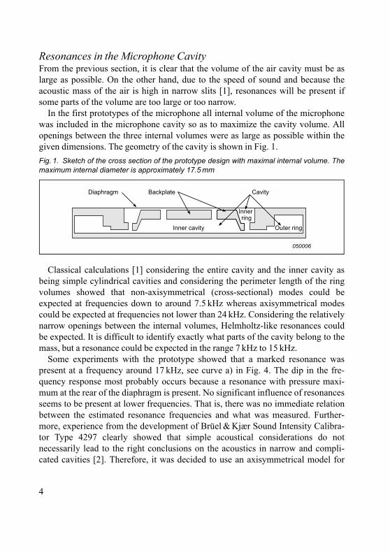
In the first prototypes of the microphone all internal volume of the microphonewas included in the microphone cavity so as to maximize the cavity volume. Allopenings between the three internal volumes were as large as possible within thegiven dimensions. The geometry of the cavity is shown in Fig. 1.

Classical calculations [1] considering the entire cavity and the inner cavity asbeing simple cylindrical cavities and considering the perimeter length of the ringvolumes showed that non-axisymmetrical (cross-sectional) modes could beexpected at frequencies down to around 7.5 kHz whereas axisymmetrical modescould be expected at frequencies not lower than 24 kHz. Considering the relativelynarrow openings between the internal volumes, Helmholtz-like resonances couldbe expected. It is difficult to identify exactly what parts of the cavity belong to themass, but a resonance could be expected in the range 7 kHz to 15 kHz.

Some experiments with the prototype showed that a marked resonance waspresent at a frequency around 17 kHz, see curve a) in Fig. 4. The dip in the fre-quency response most probably occurs because a resonance with pressure maxi-mum at the rear of the diaphragm is present. No significant influence of resonancesseems to be present at lower frequencies. That is, there was no immediate relationbetween the estimated resonance frequencies and what was measured. Further-more, experience from the development of Brüel & Kjær Sound Intensity Calibra-tor Type 4297 clearly showed that simple acoustical considerations do notnecessarily lead to the right conclusions on the acoustics in narrow and compli-cated cavities [2]. Therefore, it was decided to use an axisymmetrical model for

Fig. 1. Sketch of the cross section of the prototype design with maximal internal volume. Themaximum internal diameter is approximately 17.5 mm

Diaphragm Backplate Cavity

Inner cavity Outer ring

Inner ring

050006

4

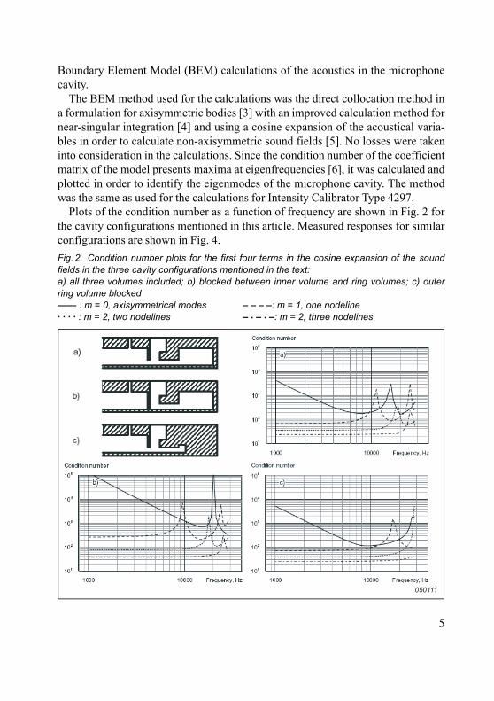
Boundary Element Model (BEM) calculations of the acoustics in the microphonecavity.

The BEM method used for the calculations was the direct collocation method ina formulation for axisymmetric bodies [3] with an improved calculation method fornear-singular integration [4] and using a cosine expansion of the acoustical varia-bles in order to calculate non-axisymmetric sound fields [5]. No losses were takeninto consideration in the calculations. Since the condition number of the coefficientmatrix of the model presents maxima at eigenfrequencies [6], it was calculated andplotted in order to identify the eigenmodes of the microphone cavity. The methodwas the same as used for the calculations for Intensity Calibrator Type 4297.

Plots of the condition number as a function of frequency are shown in Fig. 2 forthe cavity configurations mentioned in this article. Measured responses for similarconfigurations are shown in Fig. 4.Fig. 2. Condition number plots for the first four terms in the cosine expansion of the soundfields in the three cavity configurations mentioned in the text: a) all three volumes included; b) blocked between inner volume and ring volumes; c) outerring volume blocked�� : m = 0, axisymmetrical modes � � � �: m = 1, one nodeline· · · · : m = 2, two nodelines � · � · �: m = 2, three nodelines

050111

5

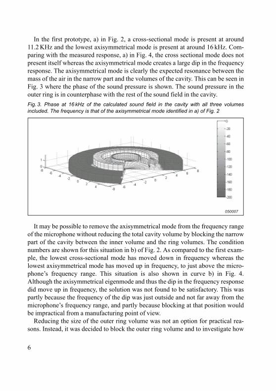
In the first prototype, a) in Fig. 2, a cross-sectional mode is present at around11.2 KHz and the lowest axisymmetrical mode is present at around 16 kHz. Com-paring with the measured response, a) in Fig. 4, the cross sectional mode does notpresent itself whereas the axisymmetrical mode creates a large dip in the frequencyresponse. The axisymmetrical mode is clearly the expected resonance between themass of the air in the narrow part and the volumes of the cavity. This can be seen inFig. 3 where the phase of the sound pressure is shown. The sound pressure in theouter ring is in counterphase with the rest of the sound field in the cavity.

It may be possible to remove the axisymmetrical mode from the frequency rangeof the microphone without reducing the total cavity volume by blocking the narrowpart of the cavity between the inner volume and the ring volumes. The conditionnumbers are shown for this situation in b) of Fig. 2. As compared to the first exam-ple, the lowest cross-sectional mode has moved down in frequency whereas thelowest axisymmetrical mode has moved up in frequency, to just above the micro-phone�s frequency range. This situation is also shown in curve b) in Fig. 4.Although the axisymmetrical eigenmode and thus the dip in the frequency responsedid move up in frequency, the solution was not found to be satisfactory. This waspartly because the frequency of the dip was just outside and not far away from themicrophone�s frequency range, and partly because blocking at that position wouldbe impractical from a manufacturing point of view.

Reducing the size of the outer ring volume was not an option for practical rea-sons. Instead, it was decided to block the outer ring volume and to investigate how

Fig. 3. Phase at 16 kHz of the calculated sound field in the cavity with all three volumesincluded. The frequency is that of the axisymmetrical mode identified in a) of Fig. 2

050007

6

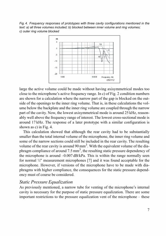
large the active volume could be made without having axisymmetrical modes tooclose to the microphone�s active frequency range. In c) of Fig. 2 condition numbersare shown for a calculation where the narrow part of the gap is blocked on the out-side of the openings to the inner ring volume. That is, in these calculations the vol-ume below the backplate and the inner ring volume are coupled through the narrowpart of the cavity. Now, the lowest axisymmetrical mode is around 25 kHz, reason-ably well above the frequency range of interest. The lowest cross-sectional mode isaround 17 kHz. The response of a later prototype with a similar configuration isshown as c) in Fig. 4.

This calculation showed that although the rear cavity had to be substantiallysmaller than the total internal volume of the microphone, the inner ring volume andsome of the narrow sections could still be included in the rear cavity. The resultingvolume of the rear cavity is around 90 mm3. With the equivalent volume of the dia-phragm compliance of around 7.5 mm3, the resulting static pressure dependency ofthe microphone is around �0.007 dB/kPa. This is within the range normally seenfor normal ½″ measurement microphones [7] and it was found acceptable for themicrophone. However, if versions of the microphone have to be made with dia-phragms with higher compliance, the consequences for the static pressure depend-ency must of course be considered.

Static Pressure EqualizationAs previously mentioned, a narrow tube for venting of the microphone�s internalcavity is necessary for the purpose of static pressure equalization. There are someimportant restrictions to the pressure equalization vent of the microphone � these

Fig. 4. Frequency responses of prototypes with three cavity configurations mentioned in thetext: a) all three volumes included; b) blocked between inner volume and ring volumes; c) outer ring volume blocked

050112

7

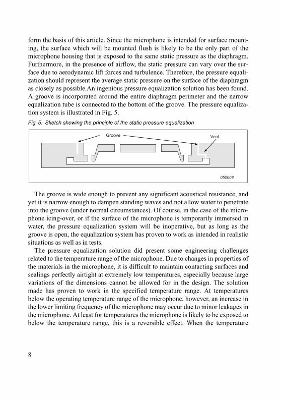
form the basis of this article. Since the microphone is intended for surface mount-ing, the surface which will be mounted flush is likely to be the only part of themicrophone housing that is exposed to the same static pressure as the diaphragm.Furthermore, in the presence of airflow, the static pressure can vary over the sur-face due to aerodynamic lift forces and turbulence. Therefore, the pressure equali-zation should represent the average static pressure on the surface of the diaphragmas closely as possible.An ingenious pressure equalization solution has been found.A groove is incorporated around the entire diaphragm perimeter and the narrowequalization tube is connected to the bottom of the groove. The pressure equaliza-tion system is illustrated in Fig. 5.

The groove is wide enough to prevent any significant acoustical resistance, andyet it is narrow enough to dampen standing waves and not allow water to penetrateinto the groove (under normal circumstances). Of course, in the case of the micro-phone icing-over, or if the surface of the microphone is temporarily immersed inwater, the pressure equalization system will be inoperative, but as long as thegroove is open, the equalization system has proven to work as intended in realisticsituations as well as in tests.

The pressure equalization solution did present some engineering challengesrelated to the temperature range of the microphone. Due to changes in properties ofthe materials in the microphone, it is difficult to maintain contacting surfaces andsealings perfectly airtight at extremely low temperatures, especially because largevariations of the dimensions cannot be allowed for in the design. The solutionmade has proven to work in the specified temperature range. At temperaturesbelow the operating temperature range of the microphone, however, an increase inthe lower limiting frequency of the microphone may occur due to minor leakages inthe microphone. At least for temperatures the microphone is likely to be exposed tobelow the temperature range, this is a reversible effect. When the temperature

Fig. 5. Sketch showing the principle of the static pressure equalization

050008

Groove Vent

8

reverts to within the operating temperature range, the lower limiting frequencyreverts to its initial value.

Influence of AirflowObviously, a microphone for sound pressure measurements in the presence ofrapid airflow must not, by itself, produce any noise due to the airflow. The surfaceof the microphone must be as flat as possible and have no recesses or obstaclesthat can generate noise in the presence of the airflow. The surface of the micro-phone should also be flush with the surface it is mounted in. For applications onaircraft surfaces the microphone must be embedded into the surface, whereas forapplications with more moderate wind speeds such as automobile surfaces, themicrophone does not necessarily have to be embedded in the surface in order toavoid wind generated noise, as long as there are no sharp edges on the mounting.

The flatness of the microphone is achieved by welding the diaphragm directly ontop of its carrying surface. In this way, the diaphragm can be totally flush with themicrophone housing. In order to avoid accidental destruction of the diaphragm,however, it is recessed a few hundredths of a millimeter relative to the rest of thesurface. The groove for pressure equalization is positioned just outside the weld-ing, so using this method, the microphone is unlikely to have any impact on the air-flow.

For applications where the microphone does not have to be embedded in the sur-face, different mounting flanges have been designed that form a smooth transitionfrom the surface of the microphone to the surrounding surface. These flanges aremade slightly flexible so that they can be mounted easily on moderately curved sur-faces.

ConclusionsIn this article the solutions to some acoustical challenges in the practical design ofa special microphone have been presented with special emphasis on the influenceof static pressure variations.

Axisymmetrical modes present in the rear cavity of a microphone have a signifi-cant impact on its response, whereas non-axisymmetrical modes seem to be lesssignificant. The cavity must be designed so that no axisymmetrical wave patternsare present in the useful frequency range of the microphone.

The solutions for static pressure equalization and minimisation of wind-inducednoise have been presented. The combinations of classical calculations, BEM calcu-

9

lations and common sense considerations have led to a successful design of themicrophone for surface mounting.

AcknowledgementsThe author wishes to thank all his colleagues at Brüel & Kjær who have partici-pated in the development of the Surface Microphone, especially Niels Eirby,Anders Eriksen, Johan Gramtorp, Jens Ole Gulløv, Bin Liu and Børge Nordstrandof the microphone development department whose combined work has led to thesuccessful design of the Surface Microphone.

References[1] See, for example, Beranek L.L., �Acoustics�, Acoust. Soc. Am., Part XIII,

Acoustic Elements, (1996).

[2] Olsen E.S., Cutanda V., Gramtorp J., Eriksen A., �Calculating the SoundField in an Acoustic Intensity Probe Calibrator � a Practical Utilization ofBoundary Element Modeling�, Proceedings of the 8th InternationationalConference on Sound and Vibration, Hong Kong (2001).

[3] Seybert A.F., Soenarko B., Rizzo F.J., Shippy D.J., �A Special IntegralEquation Formulation for Acoustic Radiation and Scattering for Axisym-metric Bodies and Boundary Conditions�, J. Acoust. Soc. Am., 80, 1241-1247 (1986).

[4] Cutanda V., Juhl P.M., Jacobsen F., �On the Modeling of Narrow Gaps usingthe Standard Boundary Element Method�, J. Acoust. Soc. Am., 109, 1296-1303 (2001).

[5] Juhl P.M., �An Axisymmetric Integral Equation Formulation for Free SpaceNon Axisymmetric Radiation and Scattering of a Known Incident Wave�, J. Sound Vib., 163, 397-406 (1993).

[6] Bai M.R., �Study of Acoustic Resonance in Enclosures using EigenanalysisBased on Boundary Element Methods�, J. Acoust. Soc. Am., 91, 2529-2538(1992).

[7] Brüel & Kjær, �Microphone Handbook for the Falcon Range® of Micro-phone Products�, Brüel & Kjær (1995).

10

Combined NAH and Beamforming Using the Same Array

J. Hald

AbstractThis article deals with the problem of how to design a microphone array that per-forms well for measurements using both Nearfield Acoustical Holography (NAH)and Beamforming (BF), as well as how to perform NAH processing on irregulararray measurements. NAH typically provides calibrated sound intensity maps,while BF provides unscaled maps. The article also describes a method to performsound intensity scaling of the BF maps in such a way that area-integration pro-vides a good estimate of the sub-area sound power. Results from a set of loud-speaker measurements are presented.

RésuméCet article traite de la difficulté de concevoir une antenne microphonique dédiéetout à la fois aux mesures d�imagerie acoustique par holographie en champ proche(NAH) et beamforming (BF) et au traitement NAH des mesures obtenues aumoyen d�antennes de géométrie irrégulière. La technique NAH procure typique-ment une cartographie calibrée de l�intensité acoustique tandis que l�approche BFfournit des cartes dépourvues d�échelle. Cet article décrit également une méthodede mise à l�échelle des cartes d�intensité acoustique BF de telle manière que l�inté-gration surfacique conduise à une juste estimation de la puissance acoustique parélément de surface. Avec une présentation des résultats d�un mesurage réalisé avecun jeu de haut-parleurs.

ZusammenfassungDieser Artikel beschäftigt sich mit dem Problem, wie sich ein Mikrofonarray kon-struieren lässt, das sich für Messungen mit akustischer Nahfeldholographie (NAH)und Beamforming (BF) eignet, sowie damit, wie sich Messungen mit irregulärenArrays für NAH aufbereiten lassen. NAH liefert in der Regel kalibrierte Schallin-tensitäts-Kartierungen, während BF nichtskalierte Kartierungen liefert. Der Artikel

11

beschreibt auch eine Methode zur Skalierung der Schallintensität auf BF-Kartie-rungen, bei der die Integration über die Fläche eine gute Abschätzung der Teil-schallleistungen ergibt. Es werden Ergebnisse von einer Messserie anLautsprechern vorgestellt.

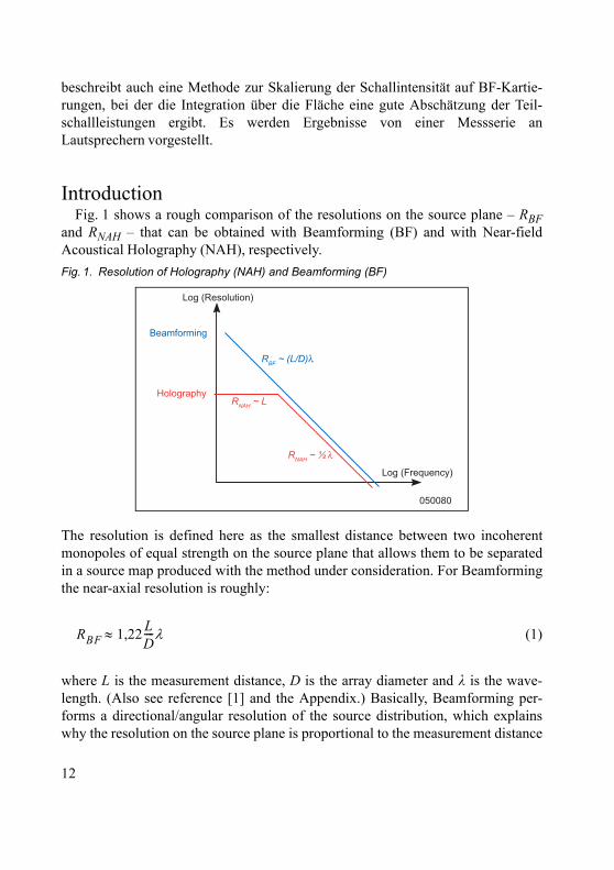
IntroductionFig. 1 shows a rough comparison of the resolutions on the source plane � RBF

and RNAH � that can be obtained with Beamforming (BF) and with Near-fieldAcoustical Holography (NAH), respectively.

The resolution is defined here as the smallest distance between two incoherentmonopoles of equal strength on the source plane that allows them to be separatedin a source map produced with the method under consideration. For Beamformingthe near-axial resolution is roughly:

(1)

where L is the measurement distance, D is the array diameter and k is the wave-length. (Also see reference [1] and the Appendix.) Basically, Beamforming per-forms a directional/angular resolution of the source distribution, which explainswhy the resolution on the source plane is proportional to the measurement distance

Fig. 1. Resolution of Holography (NAH) and Beamforming (BF)

Log (Resolution)

Beamforming

HolographyRNAH ~ L

RNAH ~ ½ λ

RBF ~ (L/D)λ

Log (Frequency)

050080

RBF 1,22 LD----λ≈

12

L. Since typically, the focusing capabilities of Beamforming require that all arraymicrophones be exposed almost equally to any monopole on the source plane, themeasurement distance required is normally equal to, or greater than the arraydiameter. As a consequence, the resolution cannot be better than one wavelength(approximately), which is often not acceptable at low frequencies.

For NAH, the resolution RNAH is approximately half the wavelength at high fre-quencies, which is only a bit better than the resolution of Beamforming. But at lowfrequencies it never gets poorer than approximately the measurement distance L.By measuring very near the source using a measurement grid with a small gridspacing, NAH can reconstruct part of the evanescent waves that decay exponen-tially away from the source, [2]. This explains the superior low-frequency resolu-tion of NAH.

However, NAH requires a measurement grid with less than half wavelengthspacing at the highest frequency of interest, covering at least the full mapping area,to build up a complete local model of the sound field. This requirement makes themethod impractical at higher frequencies because too many measurement pointsare needed. To get a comparable evaluation of the number of measurement pointsneeded for BF we notice that usually the smallest possible measurement distanceL≈D is applied to get the highest spatial resolution. Since further the resolutiondeteriorates quickly beyond a 30° angle from the array axis, the effective mappingarea is only slightly larger than the array area, [1]. Fortunately, by the use of opti-mised irregular array geometries, good suppression (at least 10 dB) of ghost imagescan be achieved up to frequencies where the average element spacing is severalwavelengths, typically 3�4 wavelengths. So to map a quadratic area with a lineardimension of four wavelengths, NAH requires more than 64 measurement posi-tions, whereas Beamforming can achieve the same results with only one position.This often makes BF the only feasible solution at high frequencies.

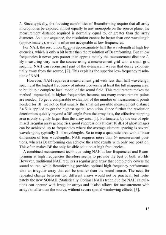
A combined measurement technique using NAH at low frequencies and Beam-forming at high frequencies therefore seems to provide the best of both worlds.However, traditional NAH requires a regular grid array that completely covers thesound source, while Beamforming provides optimal high-frequency performancewith an irregular array that can be smaller than the sound source. The need forrepeated change between two different arrays would not be practical, but fortu-nately the new SONAH (Statistically Optimal NAH) technique for NAH calcula-tions can operate with irregular arrays and it also allows for measurement witharrays smaller than the source, without severe spatial windowing effects, [3].

13

The principle of the combined measurement technique is illustrated in Fig. 2,using a new so-called �Sector Wheel Array� design, which will be explained furtherin the following chapter. Based on two recordings taken with the same array at twodifferent distances (a nearfield SONAH measurement and a BF measurement at anintermediate distance), a high-resolution source map can be obtained over a verywide frequency range. The measurement distance shown for Beamforming is verysmall � a bit larger than half the array diameter. Simulations and practical measure-ments described in this article show that with, for example, the irregular SectorWheel Array of Fig. 2, Beamforming processing works well down to that distance.

Array Designs for the Combined Measurement TechniqueConsidering first the Beamforming application, it is well known that irregular

arrays provide potentially superior performance in terms of low sidelobe level overa very wide frequency band, i.e., up to frequencies where the average microphonespacing is much larger than half the wavelength, [1]. The best performance is typi-cally achieved, if the set of two-dimensional spatial sampling intervals is non-redundant, i.e., the spacing vectors between all pairs of microphones are different.In references [4] and [1] an optimisation technique was introduced to adjust the

Fig. 2. Principle of the combined SONAH and Beamforming technique based on two meas-urements with the same array

050081

Source

Irregular array

Uniform density

1 metre diameter

60 elements

Source

1

2

• Holography (SONAH)• 12 cm distance

• 50 –1200 Hz

• Resolution ~ 12 cm

• Beamforming• 50 – 60 cm distance

• 1000 – 8000 Hz

• Resolution ~ 0.7λ

14

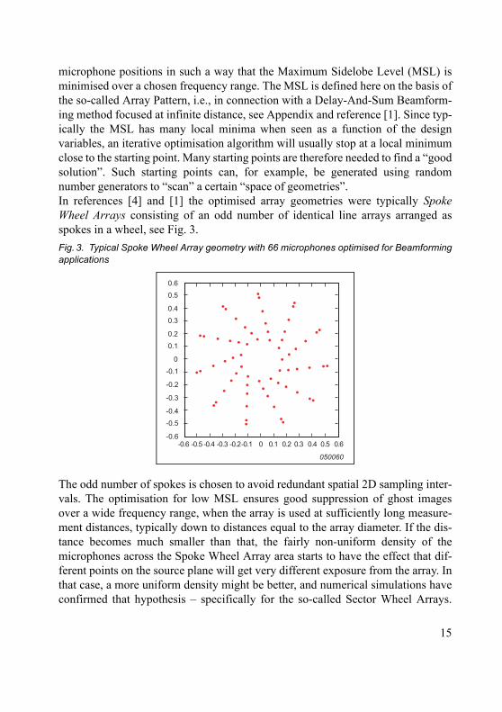
microphone positions in such a way that the Maximum Sidelobe Level (MSL) isminimised over a chosen frequency range. The MSL is defined here on the basis ofthe so-called Array Pattern, i.e., in connection with a Delay-And-Sum Beamform-ing method focused at infinite distance, see Appendix and reference [1]. Since typ-ically the MSL has many local minima when seen as a function of the designvariables, an iterative optimisation algorithm will usually stop at a local minimumclose to the starting point. Many starting points are therefore needed to find a �goodsolution�. Such starting points can, for example, be generated using randomnumber generators to �scan� a certain �space of geometries�.In references [4] and [1] the optimised array geometries were typically SpokeWheel Arrays consisting of an odd number of identical line arrays arranged asspokes in a wheel, see Fig. 3.

The odd number of spokes is chosen to avoid redundant spatial 2D sampling inter-vals. The optimisation for low MSL ensures good suppression of ghost imagesover a wide frequency range, when the array is used at sufficiently long measure-ment distances, typically down to distances equal to the array diameter. If the dis-tance becomes much smaller than that, the fairly non-uniform density of themicrophones across the Spoke Wheel Array area starts to have the effect that dif-ferent points on the source plane will get very different exposure from the array. Inthat case, a more uniform density might be better, and numerical simulations haveconfirmed that hypothesis � specifically for the so-called Sector Wheel Arrays.

Fig. 3. Typical Spoke Wheel Array geometry with 66 microphones optimised for Beamformingapplications

050060

0.6

0.5

0.4

0.3

0.2

0.1

0

-0.1

-0.2

-0.3

-0.4

-0.5

-0.6-0.6 -0.5 -0.4 -0.3 -0.2-0.1 0 0.1 0.2 0.3 0.4 0.5 0.6

15

When the same array has also to be used for near-field holography measurementsat very small measurement distances, a more uniform density is even more impor-tant. This will be covered in more detail in the following text.

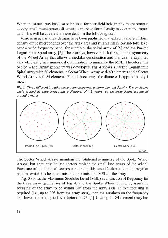
Various irregular array designs have been published that exhibit a more uniformdensity of the microphones over the array area and still maintain low sidelobe levelover a wide frequency band, for example, the spiral array of [5] and the PackedLogarithmic Spiral array, [6]. These arrays, however, lack the rotational symmetryof the Wheel Array that allows a modular construction and that can be exploitedvery efficiently in a numerical optimisation to minimise the MSL. Therefore, theSector Wheel Array geometry was developed. Fig. 4 shows a Packed LogarithmicSpiral array with 60 elements, a Sector Wheel Array with 60 elements and a SectorWheel Array with 84 elements. For all three arrays the diameter is approximately 1meter.

The Sector Wheel Arrays maintain the rotational symmetry of the Spoke WheelArrays, but angularly limited sectors replace the small line arrays of the wheel.Each one of the identical sectors contains in this case 12 elements in an irregularpattern, which has been optimised to minimise the MSL of the array.

Fig. 5 shows the Maximum Sidelobe Level (MSL) as a function of frequency forthe three array geometries of Fig. 4, and the Spoke Wheel of Fig. 3, assumingfocusing of the array to be within 30° from the array axis. If free focusing isrequired (i.e., up to 90° from the array axis), then the numbers on the frequencyaxis have to be multiplied by a factor of 0.75, [1]. Clearly, the 84-element array has

Fig. 4. Three different irregular array geometries with uniform element density. The enclosingcircle around all three arrays has a diameter of 1.2 meters, so the array diameters are allaround 1 meter

050061

Sector Wheel (84)Sector Wheel (60)Packed Log. Spiral (60)

16

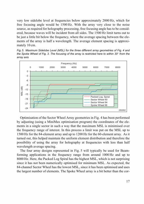
very low sidelobe level at frequencies below approximately 2000 Hz, which forfree focusing angle would be 1500 Hz. With the array very close to the noisesource, as required for holography processing, free focusing angle has to be consid-ered, because waves will be incident from all sides. The 1500 Hz limit turns out tobe just a little bit below the frequency, where the average spacing between the ele-ments of the array is half a wavelength. The average element spacing is approxi-mately 10 cm.

Optimisation of the Sector Wheel Array geometries in Fig. 4 has been performedby adjusting (using a MiniMax optimisation program) the coordinates of the ele-ments in a single sector in such a way that the maximum MSL is minimised overthe frequency range of interest. In this process a limit was put on the MSL up to1500 Hz for the 84-element array and up to 1200 Hz for the 60-element array. As itturned out, this helped maintain the uniform element distribution and therefore thepossibility of using the array for holography at frequencies with less than halfwavelength average spacing.

The four array designs represented in Fig. 5 will typically be used for Beam-forming applications in the frequency range from around 1000 Hz and up to8000 Hz. Here, the Packed Log Spiral has the highest MSL, which is not surprisingsince it has not been numerically optimised for minimum MSL. As expected, the84-channel Sector Wheel has the lowest MSL, since it has been optimised and usesthe largest number of elements. The Spoke Wheel array is a bit better than the cor-

Fig. 5. Maximum Sidelobe Level (MSL) for the three different array geometries of Fig. 4 andthe Spoke Wheel of Fig. 3. The focusing of the array is restricted here to within 30° from thearray axis

Packed Log. Spiral

Sector Wheel 60

Sector Wheel 84

Spoke Wheel 66

0 1000 2000 3000 4000 5000 6000 7000 8000

-18

-15

-12

-9

-6

-3

0

-21

-24050062

Frequency (Hz)

MS

L (

dB

)

17

responding 60-element Sector Wheel over the Beamforming frequency range. Butthe Sector Wheel is significantly better over a rather wide range of low frequencies,where it applies for SONAH holography.

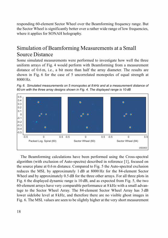
Simulation of Beamforming Measurements at a Small Source DistanceSome simulated measurements were performed to investigate how well the threeuniform arrays of Fig. 4 would perform with Beamforming from a measurementdistance of 0.6 m, i.e., a bit more than half the array diameter. The results areshown in Fig. 6 for the case of 5 uncorrelated monopoles of equal strength at8000 Hz.

The Beamforming calculations have been performed using the Cross-spectralalgorithm (with exclusion of Auto-spectra) described in reference [1], focused onthe source plane at 0.6 m distance. Compared to Fig. 5 the Auto-spectral exclusionreduces the MSL by approximately 1 dB at 8000 Hz for the 84-element SectorWheel and by approximately 0.5 dB for the three other arrays. For all three plots inFig. 6 the displayed dynamic range is 10 dB, and as expected from Fig. 5, the two60-element arrays have very comparable performance at 8 kHz with a small advan-tage to the Sector Wheel Array. The 84-element Sector Wheel Array has 3 dBlower sidelobe level at 8 kHz, and therefore there are no visible ghost images inFig. 6. The MSL values are seen to be slightly higher at the very short measurement

Fig. 6. Simulated measurements on 5 monopoles at 8 kHz and at a measurement distance of60 cm with the three array designs shown in Fig. 4. The displayed range is 10 dB

0.5

0.5

0.4

0.3

0.2

0.1

0

0

-0.1

-0.2

-0.3

-0.4

-0.5

-0.5 0.5

Packed Log. Spiral (60) Sector Wheel (60) Sector Wheel (84)

0-0.5 0.50-0.5

050063

18

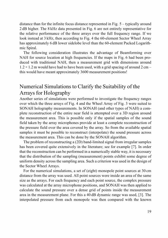
distance than for the infinite focus distance represented in Fig. 5 � typically around2 dB higher. The 8 kHz data presented in Fig. 6 are not entirely representative forthe relative performance of the three arrays over the full frequency range. If welook instead at 3 kHz, then according to Fig. 4 the 60-element Sector Wheel Arrayhas approximately 6 dB lower sidelobe level than the 60-element Packed Logarith-mic Spiral.

The following consideration illustrates the advantage of Beamforming overNAH for source location at high frequencies. If the maps in Fig. 6 had been pro-duced with traditional NAH, then a measurement grid with dimensions around1.2 × 1.2 m would have had to have been used, with a grid spacing of around 2 cm �this would have meant approximately 3600 measurement positions!

Numerical Simulations to Clarify the Suitability of the Arrays for HolographyAnother series of simulations were performed to investigate the frequency rangesover which the three arrays of Fig. 4 and the Wheel Array of Fig. 3 were suited toSONAH holography measurements. In SONAH (and other types of NAH) a com-plete reconstruction of the entire near field is attempted over a 3D region aroundthe measurement area. This is possible only if the spatial samples of the soundfield taken by the array microphones provide at least a complete reconstruction ofthe pressure field over the area covered by the array. So from the available spatialsamples it must be possible to reconstruct (interpolate) the sound pressure acrossthe measurement area. This can be done by the SONAH algorithm.

The problem of reconstructing a (2D) band-limited signal from irregular sampleshas been covered quite extensively in the literature; see for example [7]. In orderthat the reconstruction can be performed in a numerically stable way, it is necessarythat the distribution of the sampling (measurement) points exhibit some degree ofuniform density across the sampling area. Such a criterion was used in the design ofthe Sector Wheel Arrays.

For the numerical simulations, a set of (eight) monopole point sources at 30 cmdistance from the array was used. All point sources were inside an area of the samesize as the arrays. For each frequency and each point source, the complex pressurewas calculated at the array microphone positions, and SONAH was then applied tocalculate the sound pressure over a dense grid of points inside the measurementarea in the measurement plane. For this a 40 dB dynamic range was used, [3]. Theinterpolated pressure from each monopole was then compared with the known

19

pressure from the same monopole, and the Relative Average Error was estimated ateach frequency as the ratio between a sum of squared errors and a correspondingsum of squared true pressure values. The summation was, in both cases, over allinterpolation points and all sources.

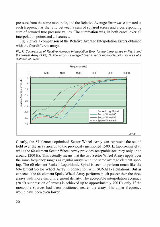
Fig. 7 gives a comparison of the Relative Average Interpolation Errors obtainedwith the four different arrays.

Clearly, the 84-element optimised Sector Wheel Array can represent the soundfield over the array area up to the previously mentioned 1500 Hz (approximately),while the 60-element Sector Wheel Array provides acceptable accuracy only up toaround 1200 Hz. This actually means that the two Sector Wheel Arrays apply overthe same frequency ranges as regular arrays with the same average element spac-ing. The 60-element Packed Logarithmic Spiral is seen to perform much like the60-element Sector Wheel Array in connection with SONAH calculations. But asexpected, the 66-element Spoke Wheel Array performs much poorer then the threearrays with more uniform element density. The acceptable interpolation accuracy(20 dB suppression of errors) is achieved up to approximately 700 Hz only. If themonopole sources had been positioned nearer the array, this upper frequencywould have been even lower.

Fig. 7. Comparison of Relative Average Interpolation Error for the three arrays in Fig. 4 andthe Wheel Array of Fig. 3. The error is averaged over a set of monopole point sources at adistance of 30 cm

Packed Log. Spiral

Sector Wheel 60

Sector Wheel 84

Spoke Wheel 66

0 500 1000 1500 2000 2500 30000

-30

-25

-20

-15

-10

-5

0

-35

-40

050064

Frequency (Hz)

Re

lative

Ave

rag

e e

rro

r (d

B)

20

Intensity Scaling of Beamformer OutputWhen combining low-frequency results obtained with SONAH and high-fre-quency results obtained with Beamforming it is desirable to have the results scaledin the same way. This is not straightforward, however, as will be apparent from thefollowing description of the basic output from SONAH and Beamforming.

Based on the measured pressure data, SONAH builds a sound field model validwithin a 3D region around the array, and using that model it is possible to map anysound field parameter. Typically the sound intensity normal to the array plane iscalculated to get the information about source location and strength. Since themeasurement is taken very near the sources, the energy radiated in any directionwithin a 2p solid angle will be captured and included with the sound intensity andsound power estimates.

Beamforming, on the other hand, is based on a measurement taken at some inter-mediate distance from the sources where only a fraction of the 2p solid angle iscovered by the array. Rather than estimating sound field parameters for the sourceregion, directional filtering is performed on the sound field incident towards thearray. As a result only the relative contributions to the sound pressure at the arrayposition from different directions is obtained. Reference [8] describes a scaling ofthe output that allows the contribution at the array position from specific sourceareas to be read directly from the Beamformer maps. This is, of course, meaningfulonly if the pressure distribution across the array area from the various partialsources is fairly constant, which will be true if the array covers a relatively smallsolid angle as seen from the sources.

But in the context of this article, we wish to take BF measurements as close aspossible to the source area, in order to obtain the best possible spatial resolution. Asa consequence, the radiation into a rather large fraction of the 2π solid angle ismeasured. We should therefore be in a better position to get information about (forexample) the sound power radiated through the source plane. If we want to scalethe Beamformer output in such a way that the scaled map represents the sourcestrength (in some way) it seems logical to scale it as active sound intensity, becausethat quantity represents the radiation towards the array and into the far-field region.Nearfield pressure contains evanescent components that are not picked up by thearray.

The Appendix describes the derivation of a method to scale the output from aDelay-And-Sum Beamformer in such a way that area integration of the scaled out-put provides a good estimate of the sub-area sound power. For that reason it is nat-ural to use the term �Sound Intensity Scaling� about the method. The derivation is

21

performed looking at a single monopole point source in the far-field region, andassuming that the array provides a good angular resolution, i.e., assuming the main-lobe covers only a small solid angle. An evaluation is then given of the errors intro-duced by the far-field assumption and the assumption of a narrow mainlobe. This isdone both for Delay-And-Sum processing and for the Cross-spectral algorithmwith exclusion of Auto-spectra. The main conclusions are for the 60-element Sec-tor Wheel Array of Fig. 4 and for frequencies above 1200 Hz:

1) The error is less than 0.4 dB when using a measurement distance not smallerthan the array diameter.

2) At smaller measurement distances the error increases, but it does not exceedapproximately 0.6 dB when the distance is larger than 0.6 times the arraydiameter.

In the Appendix it is argued that if the scaling works for a single omni-directionalsource, then it holds also for a set of incoherent monopole sources in the sameplane. If sources are partially coherent and/or if single sources are not omni-direc-tional, then because of the limited angular coverage of the array, accurate soundpower estimation cannot possibly be obtained. Fortunately, many real-worldsound sources tend to have low spatial coherence in the frequency range whereBeamforming will be used in the combined NAH/BF method.

The derivation of the scaling is based on matching the area-integrated map withthe known sound power for a monopole sound source. In the derivation, area inte-gration was performed only over the hot spot corresponding to the mainlobe of theBeamformer. At high frequencies many sidelobes will typically be within the map-ping area, and it turns out that area-integration over a large number of sidelobeswill typically contribute significantly to the sound power. This effect can beavoided in practice by the use of a finite dynamic range during the area integration,typically around 10 dB. A frequency dependent adjustment of the integration areato match the resolution is not practical.

The measurement results to be presented in the following section will show theinfluence of measurement distance, size of the power integration area and of thepresence of more than a single source. Also, the sound power estimates will becompared with sound power data obtained from sound intensity maps measuredwith a sound intensity probe.

22

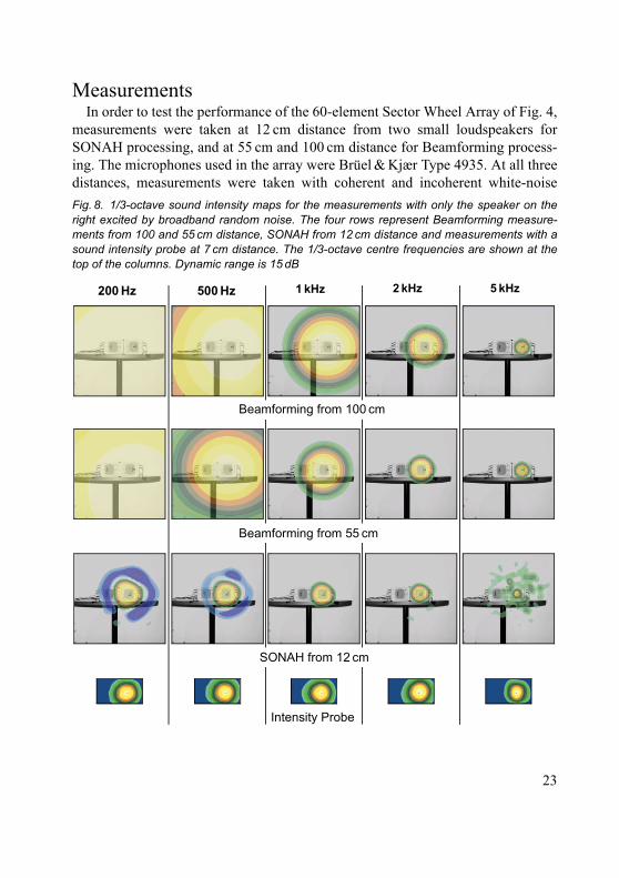
MeasurementsIn order to test the performance of the 60-element Sector Wheel Array of Fig. 4,

measurements were taken at 12 cm distance from two small loudspeakers forSONAH processing, and at 55 cm and 100 cm distance for Beamforming process-ing. The microphones used in the array were Brüel & Kjær Type 4935. At all threedistances, measurements were taken with coherent and incoherent white-noiseFig. 8. 1/3-octave sound intensity maps for the measurements with only the speaker on theright excited by broadband random noise. The four rows represent Beamforming measure-ments from 100 and 55 cm distance, SONAH from 12 cm distance and measurements with asound intensity probe at 7 cm distance. The 1/3-octave centre frequencies are shown at thetop of the columns. Dynamic range is 15 dB

500 Hz 1 kHz200 Hz 2 kHz 5 kHz

SONAH from 12 cm

Beamforming from 55 cm

Intensity Probe

Beamforming from 100 cm

23

excitation of the two speakers and also with only one speaker excited. For each ofthese three excitations, a scan was performed approximately 7 cm in front of thetwo loudspeakers with a Brüel & Kjær sound intensity probe Type 3599. The twospeakers were identical small PC units with drivers of diameter 7 cm and they weremounted with 17 cm between the centers of the drivers. The Beamforming process-ing was performed with the Cross-spectral algorithm with exclusion of Auto-spec-tra, [1].

Fig. 8 shows 1/3-octave sound intensity maps for the measurements with onlythe speaker on the right excited. The arrangement of the speaker can be seen insome of the contour plots.

The four rows of contour plots represent the Beamforming measurements takenfrom a distance of 100 cm and 50 cm, the SONAH measurements taken from 12 cmdistance and the measurements taken with an intensity probe from a distance of7 cm. For the first three rows (representing Beamforming and SONAH results) thesound intensity has been estimated in the source plane over an area of approximatesize 80 cm × 80 cm, while the last row shows the sound intensity measured 7 cmfrom the plane of the speakers over an area of size 36 cm × 21 cm. All plots show a15 dB dynamic range from the maximum level, with 1.5 dB steps between the col-ours. Yellow/orange/green colours represent outward intensity and blue colors rep-resent inward intensity. The absolute levels will be presented subsequently througharea integrated sound power data.

The resolution obtained with Beamforming and SONAH is in good agreementwith the expectations as shown in Fig. 1. The bend on the resolution curve forSONAH is in this case at approximately 1500 Hz, being determined by ½k = Lwhere L is the measurement distance and k is the wavelength. Clearly, at low fre-quencies the Beamforming resolution is very poor, while above approximately1.5 kHz it is approximately as good as that obtained with the sound intensity probe.SONAH provides good resolution over the entire frequency range, but aboveapproximately 1200 Hz, the average spacing of the microphone grid is too large toreconstruct the sound pressure variation across the measurement area. As a result,distortions will slowly appear as frequency increases, and more evidently � thelevel will be underestimated as can be seen in the sound power spectra of Fig. 11and Fig. 12. The combined method using SONAH up to 1250 Hz and Beamform-ing at higher frequencies provides good resolution at all frequencies, and the soundpower estimate is also good as shown in Fig. 11 and Fig. 12. So two recordingstaken with the Sector Wheel array at two different distances can provide the infor-mation obtained with a time consuming scan with an intensity probe (104 positions

24

for the small plots in Fig. 8). In addition, many other types of analysis can be per-formed based on the same data, such as transient analysis of radiation phenomena.

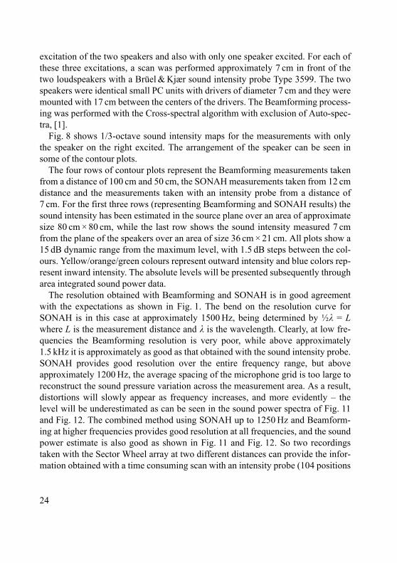
As mentioned previously, the sound intensity scaling of the output from Beam-forming is defined in such a way that area integration over the mainlobe area willprovide a good estimate of the sound power from a monopole point source. Fig. 9depicts the 1/3-octave sound power spectra for the single speaker obtained from the

scan with the sound intensity probe and from the Beamforming measurement at55 cm distance. The intensity probe measurement has been integrated over the fullmeasurement area shown in Fig. 8. Two spectra are shown for the sound powerobtained with the Beamforming measurement: one obtained by integration over thefull mapping area; another obtained by integration over a small rectangular areawith x- and y-dimensions equal to the mainlobe diameter and centered at theknown point source position. The radius of the mainlobe is 1.22kL/D, where k andL are wavelength and measurement distance (55 cm) as defined above, and where

Fig. 9. 1/3-octave sound power spectra for the single speaker measurement. The intensityprobe map has been integrated over the entire mapping area shown in Fig. 8. The Beamform-ing measurement, taken at a distance of 55 cm, has been integrated over the full mappingarea and over the mainlobe area only

Intensity Probe

BF, 55 cm, Full area

BF, 55 cm, Small area

160 200 250 315 400 500 630 800 1000 1250 1600 2000 2500 3150 4000 5000

55

60

65

70

75

80

50

45

050068Frequency (Hz)

So

un

d P

ow

er

(dB

)

25

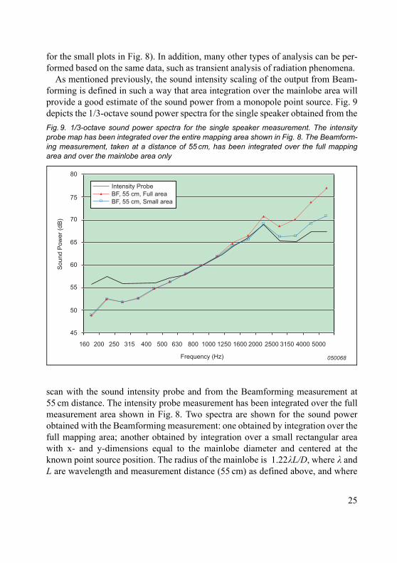
D is the array diameter of approximately 1 m, refer to equation (A15) in the Appen-dix. At low frequencies the mainlobe is larger than the entire mapping area of 0.8 mby 0.8 m, and therefore the two Beamforming spectra are identical. Here, the soundpower is underestimated, because the power outside the mapping area is notincluded, and also the assumptions made for the sound intensity scaling fail to hold,refer to the Appendix. At high frequencies the power estimated by Beamforming istoo high, even when the integration covers the mainlobe area only. This is mainlybecause the loudspeaker is no longer omni-directional as assumed in the scaling,but concentrates the radiation in the axial direction, towards the array. At 5 kHz thediameter of the driver unit is approximately one wavelength. Another reason forthe over-estimation could be the tendency of the intensity scaling to overestimatewhen the measurement distance is very small, see Fig. A3. Looking at the soundpower obtained by integration over the entire mapping area, it is even higher at thehigh frequencies. The reason is that sidelobes (ghost images) contribute signifi-cantly when the integration area is much larger than the mainlobe area, even whenthe array has good sidelobe suppression as the present Sector Wheel array. Fig. 10. 1/3-octave sound power spectra for the single speaker measurement. Again theintensity probe result is included. But now the results from Beamforming measurements at adistance of 55 cm and 100 cm are included. For both of these, the sound power integrationcovers the entire mapping area

Intensity Probe

BF, 55 cm, Full area

BF, 100 cm, Full area

160 200 250 315 400 500 630 800 1000 1250 1600 2000 2500 3150 4000 5000

55

60

65

70

75

80

50

45

050069Frequency (Hz)

So

un

d P

ow

er

(dB

)

26

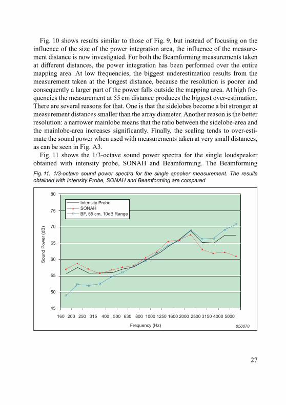
Fig. 10 shows results similar to those of Fig. 9, but instead of focusing on theinfluence of the size of the power integration area, the influence of the measure-ment distance is now investigated. For both the Beamforming measurements takenat different distances, the power integration has been performed over the entiremapping area. At low frequencies, the biggest underestimation results from themeasurement taken at the longest distance, because the resolution is poorer andconsequently a larger part of the power falls outside the mapping area. At high fre-quencies the measurement at 55 cm distance produces the biggest over-estimation.There are several reasons for that. One is that the sidelobes become a bit stronger atmeasurement distances smaller than the array diameter. Another reason is the betterresolution: a narrower mainlobe means that the ratio between the sidelobe-area andthe mainlobe-area increases significantly. Finally, the scaling tends to over-esti-mate the sound power when used with measurements taken at very small distances,as can be seen in Fig. A3.

Fig. 11 shows the 1/3-octave sound power spectra for the single loudspeakerobtained with intensity probe, SONAH and Beamforming. The BeamformingFig. 11. 1/3-octave sound power spectra for the single speaker measurement. The resultsobtained with Intensity Probe, SONAH and Beamforming are compared

160 200 250 315 400 500 630 800 1000 1250 1600 2000 2500 3150 4000 5000

55

60

65

70

75

80

50

45

050070Frequency (Hz)

Sound P

ow

er

(dB

)

Intensity Probe

SONAH

BF, 55 cm, 10dB Range

27

measurement at 55 cm distance has been chosen, and for that measurement thesound power integration has been performed over the full sound intensity map (seeFig. 8), but using only a 10 dB range of intensity data (i.e., data points where thelevel is less than 10 dB below Peak level are ignored). The result is very close tothat obtained with integration over the mainlobe area only, see Fig. 9. Above500 Hz this leads to a good estimate of the sound power, apart from the previouslydiscussed overestimation at the highest frequencies. SONAH provides good soundpower estimates up to approximately 1.6 kHz, apart from a small overestimation(which could be due to the small measurement area that is used with the soundintensity probe). But above 1.6 kHz the sound power is increasingly underesti-mated with SONAH.

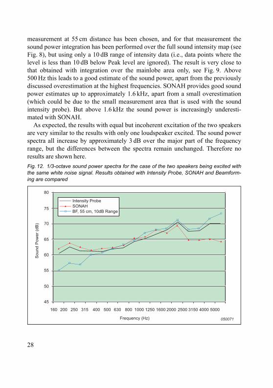
As expected, the results with equal but incoherent excitation of the two speakersare very similar to the results with only one loudspeaker excited. The sound powerspectra all increase by approximately 3 dB over the major part of the frequencyrange, but the differences between the spectra remain unchanged. Therefore noresults are shown here. Fig. 12. 1/3-octave sound power spectra for the case of the two speakers being excited withthe same white noise signal. Results obtained with Intensity Probe, SONAH and Beamform-ing are compared

Intensity Probe

SONAH

BF, 55 cm, 10dB Range

160 200 250 315 400 500 630 800 1000 1250 1600 2000 2500 3150 4000 5000

55

60

65

70

75

80

50

45

050071Frequency (Hz)

Sound P

ow

er

(dB

)

28

Equal but coherent in-phase excitation of the two loudspeakers will, on the otherhand, cause the radiation to deviate more from being omni-directional, which vio-lates the assumptions on which the intensity scaling of Beamformer maps arebased.

Fig. 12 depicts the 1/3-octave sound power spectra obtained using intensityprobe, SONAH and Beamforming with identical excitation of the two speakers.The SONAH spectrum follows the intensity probe spectrum in much the same wayas for the case of only a single speaker being excited. But the sound power obtainedfrom the scaled Beamformer map shows additional deviation in the frequencyrange from 1 kHz to 2 kHz. In that frequency range the distance between the twospeakers is between half a wavelength and one wavelength, which will focus theradiation in the axial direction. But the deviation remains within approximately2 dB from the power spectrum obtained with the sound intensity probe.

ConclusionsA new combined array measurement technique has been presented that allowsNear-field Acoustical Holography and Beamforming to be performed with thesame array. This combination can provide high-resolution noise source locationover a very broad frequency range based on two recordings with the array at twodifferent distances from the source. The key elements in the presented solution arethe use of SONAH for the holography calculation, sound intensity scaling of theBeamformer output and the use of a specially designed irregular array with uni-form element density. The optimised Sector Wheel Array is an example of anapplicable array with very high performance, particularly for the Beamformingpart. Numerical simulations and a set of measurements confirm the strengths ofthe combined method and of the Sector Wheel array design. The mentioned func-tionality is all supported in PULSE Version 9.0 from Brüel & Kjær.

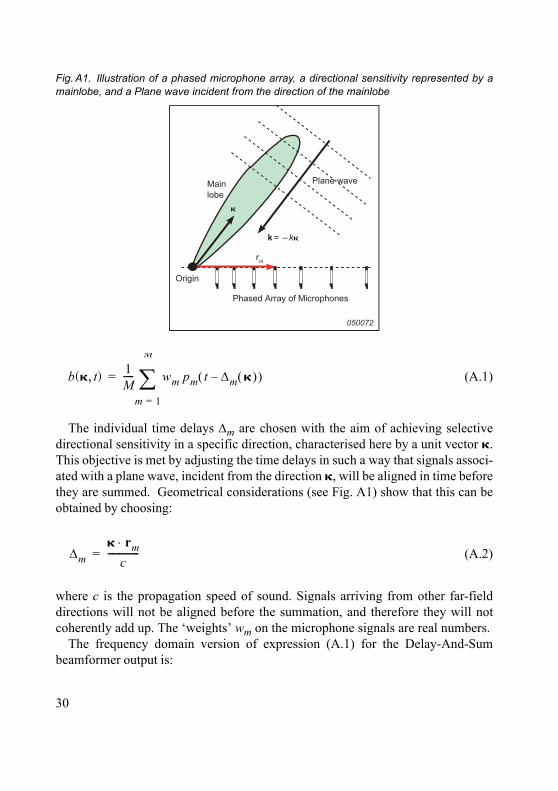
Appendix: Sound Intensity Scaling of Beamformer OutputAs illustrated in Fig. A1, we consider a planar array of M microphones at locationsrm (m = 1,2,..., M) in the xy-plane of our coordinate system. When such an array isapplied to Delay-And-Sum Beamforming, the measured pressure signals pm areindividually weighted and delayed, and then all signals are summed, [9]:

29

(A.1)

The individual time delays Δm are chosen with the aim of achieving selectivedirectional sensitivity in a specific direction, characterised here by a unit vector �.This objective is met by adjusting the time delays in such a way that signals associ-ated with a plane wave, incident from the direction �, will be aligned in time beforethey are summed. Geometrical considerations (see Fig. A1) show that this can beobtained by choosing:

(A.2)

where c is the propagation speed of sound. Signals arriving from other far-fielddirections will not be aligned before the summation, and therefore they will notcoherently add up. The �weights� wm on the microphone signals are real numbers.

The frequency domain version of expression (A.1) for the Delay-And-Sumbeamformer output is:

Fig. A1. Illustration of a phased microphone array, a directional sensitivity represented by amainlobe, and a Plane wave incident from the direction of the mainlobe

Main

lobe

Plane wave

Phased Array of Microphones

Origin

k = – k�

rm

050072

�

b � t( , ) 1M----- wm

m 1=

M

∑ pm t Δm �( )�( )=

Δm� rm⋅

c--------------=

30

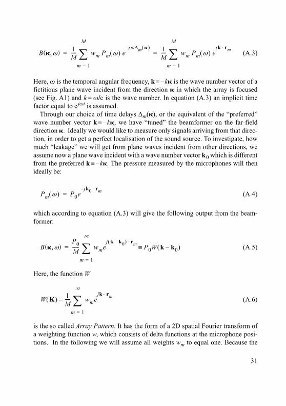
(A.3)

Here, x is the temporal angular frequency, k ≡ �k� is the wave number vector of afictitious plane wave incident from the direction � in which the array is focused(see Fig. A1) and k = x/c is the wave number. In equation (A.3) an implicit timefactor equal to e jxt is assumed.

Through our choice of time delays Δm(�), or the equivalent of the �preferred�wave number vector k ≡ �k�, we have �tuned� the beamformer on the far-fielddirection �. Ideally we would like to measure only signals arriving from that direc-tion, in order to get a perfect localisation of the sound source. To investigate, howmuch �leakage� we will get from plane waves incident from other directions, weassume now a plane wave incident with a wave number vector k0 which is differentfrom the preferred k ≡ �k�. The pressure measured by the microphones will thenideally be:

(A.4)

which according to equation (A.3) will give the following output from the beam-former:

(A.5)

Here, the function W

(A.6)

is the so called Array Pattern. It has the form of a 2D spatial Fourier transform ofa weighting function w, which consists of delta functions at the microphone posi-tions. In the following we will assume all weights wm to equal one. Because the

B � ω( , ) 1M----- wm Pm

m 1=

M

∑ ω( ) ejωΔm �( )� 1

M----- wm

m 1=

M

∑ Pm ω( ) ejk rm⋅

= =

Pm ω( ) P0ejk0� rm⋅

=

B � ω( , )P0M------ wme

j k k0�( ) rm⋅

m 1=

M

∑ P0W k k0�( )≡=

W K( ) 1M----- wme

jk rm⋅

m 1=

M

∑≡

31

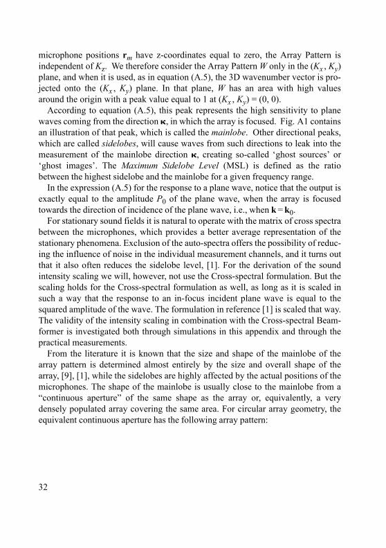
microphone positions rm have z-coordinates equal to zero, the Array Pattern isindependent of Kz. We therefore consider the Array Pattern W only in the (Kx , Ky)plane, and when it is used, as in equation (A.5), the 3D wavenumber vector is pro-jected onto the (Kx , Ky) plane. In that plane, W has an area with high valuesaround the origin with a peak value equal to 1 at (Kx , Ky) = (0, 0).

According to equation (A.5), this peak represents the high sensitivity to planewaves coming from the direction �, in which the array is focused. Fig. A1 containsan illustration of that peak, which is called the mainlobe. Other directional peaks,which are called sidelobes, will cause waves from such directions to leak into themeasurement of the mainlobe direction �, creating so-called �ghost sources� or�ghost images�. The Maximum Sidelobe Level (MSL) is defined as the ratiobetween the highest sidelobe and the mainlobe for a given frequency range.

In the expression (A.5) for the response to a plane wave, notice that the output isexactly equal to the amplitude P0 of the plane wave, when the array is focusedtowards the direction of incidence of the plane wave, i.e., when k = k0.

For stationary sound fields it is natural to operate with the matrix of cross spectrabetween the microphones, which provides a better average representation of thestationary phenomena. Exclusion of the auto-spectra offers the possibility of reduc-ing the influence of noise in the individual measurement channels, and it turns outthat it also often reduces the sidelobe level, [1]. For the derivation of the soundintensity scaling we will, however, not use the Cross-spectral formulation. But thescaling holds for the Cross-spectral formulation as well, as long as it is scaled insuch a way that the response to an in-focus incident plane wave is equal to thesquared amplitude of the wave. The formulation in reference [1] is scaled that way.The validity of the intensity scaling in combination with the Cross-spectral Beam-former is investigated both through simulations in this appendix and through thepractical measurements.

From the literature it is known that the size and shape of the mainlobe of thearray pattern is determined almost entirely by the size and overall shape of thearray, [9], [1], while the sidelobes are highly affected by the actual positions of themicrophones. The shape of the mainlobe is usually close to the mainlobe from a�continuous aperture� of the same shape as the array or, equivalently, a verydensely populated array covering the same area. For circular array geometry, theequivalent continuous aperture has the following array pattern:

32

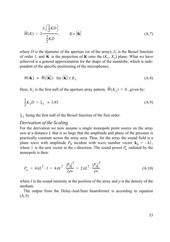
(A.7)

where D is the diameter of the aperture (or of the array), J1 is the Bessel functionof order 1, and is the projection of K onto the (Kx , Ky) plane. What we haveachieved is a general approximation for the shape of the mainlobe, which is inde-pendent of the specific positioning of the microphones,

≈ for (A.8)

Here, K1 is the first null of the aperture array pattern, , given by:

≈ 3.83 (A.9)

being the first null of the Bessel function of the first order.

Derivation of the ScalingFor the derivation we now assume a single monopole point source on the arrayaxis at a distance L that is so large that the amplitude and phase of the pressure ispractically constant across the array area. Thus, for the array the sound field is aplane wave with amplitude P0 incident with wave number vector ,where is the unit vector in the z-direction. The sound power Pa radiated by themonopole is then:

(A.10)

where I is the sound intensity at the position of the array and q is the density of themedium.

The output from the Delay-And-Sum beamformer is according to equation(A.5):

W K( ) 2J1

12---KD⎝ ⎠

⎛ ⎞

12---KD

----------------------- K K≡,=

K

W K( ) W K( ) K K1≤

W K1( ) 0=

12---K1D ξ1=

ξ1

k0 kz�=z

Pa 4πL2 I⋅ 4πL2 P02

2ρc-----------⋅ 2πL2 P0

2

ρc-----------⋅= = =

33

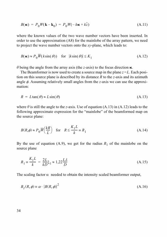
(A.11)

where the known values of the two wave number vectors have been inserted. Inorder to use the approximation (A8) for the mainlobe of the array pattern, we needto project the wave number vectors onto the xy-plane, which leads to:

for (A.12)

h being the angle from the array axis (the z-axis) to the focus direction �.The Beamformer is now used to create a source map in the plane z =L. Each posi-

tion on this source plane is described by its distance R to the z-axis and its azimuthangle φ. Assuming relatively small angles from the z-axis we can use the approxi-mation:

(A.13)

where h is still the angle to the z-axis. Use of equation (A.13) in (A.12) leads to thefollowing approximate expression for the �mainlobe� of the beamformed map onthe source plane:

for (A.14)

By the use of equation (A.9), we get for the radius R1 of the mainlobe on thesource plane

(A.15)

The scaling factor α needed to obtain the intensity scaled beamformer output,

(A.16)

B �( ) P0W k k0�( ) P0W k�� kz+( )= =

B �( ) P0W k θ( )sin( )≈ k θ( )sin K1≤

R L θ( )tan L θ( )sin≈=

B R φ( , ) P0W kRL

------⎝ ⎠⎛ ⎞≈ R

K1Lk

----------≤ R1≡

R1K1L

k----------≡ 2L

kD-------ξ1 1,22Lλ

D------≈=

BI R φ( , ) α B R φ( , ) 2⋅≡

34

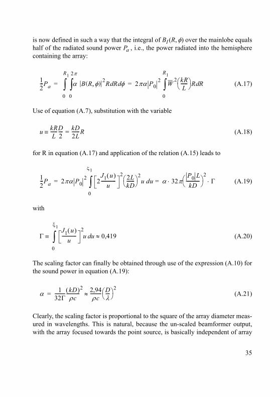
is now defined in such a way that the integral of BI (R, φ) over the mainlobe equalshalf of the radiated sound power Pa , i.e., the power radiated into the hemispherecontaining the array:

(A.17)

Use of equation (A.7), substitution with the variable

(A.18)

for R in equation (A.17) and application of the relation (A.15) leads to

(A.19)

with

(A.20)

The scaling factor can finally be obtained through use of the expression (A.10) forthe sound power in equation (A.19):

(A.21)

Clearly, the scaling factor is proportional to the square of the array diameter meas-ured in wavelengths. This is natural, because the un-scaled beamformer output,with the array focused towards the point source, is basically independent of array

12---Pa α B R φ( , ) 2R Rd φd

0

2π

∫0

R1

∫ 2πα P02 W

2

0

R1

∫ kRL------⎝ ⎠

⎛ ⎞ R Rd= =

u kRL

------D2---- kD

2L-------R=≡

12---Pa 2πα P0

2 2J1 u( )

u-------------

0

ξ1

∫2 2L

kD-------⎝ ⎠

⎛ ⎞ 2u du α 32π

P0 LkD

------------⎝ ⎠⎛ ⎞

2Γ⋅ ⋅= =

ΓJ1 u( )

u-------------

2u ud

0

ξ1

∫ 0,419≈≡

α 132Γ--------- kD( )

ρc------------

2 2,94ρc

---------- Dλ----⎝ ⎠

⎛ ⎞ 2≈=

35

geometry, but the width of the mainlobe is inversely proportional to the arraydiameter measured in wavelengths (refer to equation A.15). To maintain the area-integrated power with increasing array diameter, the scaling factor must have theproportionality mentioned above.

Evaluation of ErrorsThe major principle of the scaling is that area integration of the scaled output mustprovide a good estimate of the sub-area sound power. For that reason it is naturalto use the term �Sound Intensity Scaling� about the method. The scaling is definedfor a single omni-directional point source in such a way that area integration of thepeak created by the mainlobe equals the known radiated power from the pointsource. So by this definition the total power will be within the mainlobe radiusfrom the source position, and integration over a larger area will cause an overesti-mation of the sound power. One reason for choosing this definition is that only themainlobe has a form that depends only on the array diameter and not on all micro-phone positions. Other choices would be somewhat arbitrary, would require inte-gration over a larger area to get the total power and would need the scaling factorto depend on the particular set of microphone positions. But the influence of thesidelobes on the power integration is a drawback � if the mainlobe is rather narrowand sound power integration is performed over an area much larger than the sizeof the mainlobe on the source plane, then the level of sidelobes often present inbeamforming can contribute significantly to the power integration and cause a sig-nificant over-estimation of the sound power. The solution adopted to avoid thissignificant over-estimation is to use only a finite dynamic range of sound intensityin the area integration, typically around 10 dB. The applied dynamic range, how-ever, should depend on the MSL of the array.

The scaling was derived for a single omni-directional point source on the arrayaxis. Beyond that we have assumed the monopole to be so far away from the arraythat its sound field has the form of a plane wave across the array. Thus, we haveassumed the source to be in the far-field region relative to the array. The secondimportant assumption introduced in equations (A.13�A.14) above is that the main-lobe covers a relatively small solid angle. To investigate the effect of the last twoassumptions, a series of simulations have been performed with the 60-channel Sec-tor Wheel Array of Fig. 4 and with a single monopole point source at different dis-tances on the array axis and operating at different frequencies. The beamformingcalculation has been performed with two different beamformers:

36

1) A Delay-And-Sum beamformer focused at the finite source distance, butwithout any amplitude/distance compensation, [1].

2) The Cross-spectral beamformer with exclusion of Auto-spectra described inreference [1]. This method compensates for the amplitude variation acrossthe array of the sound pressure from a monopole on the source plane.

The output has then been scaled as sound intensity through multiplication with thescaling factor a of equation (A.21), and finally the sound power has been esti-mated by integration over a circular area with radius equal to R1 (refer to equationA.15) around the array axis.

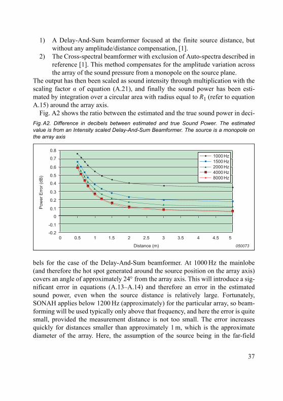
Fig. A2 shows the ratio between the estimated and the true sound power in deci-

bels for the case of the Delay-And-Sum beamformer. At 1000 Hz the mainlobe(and therefore the hot spot generated around the source position on the array axis)covers an angle of approximately 24° from the array axis. This will introduce a sig-nificant error in equations (A.13�A.14) and therefore an error in the estimatedsound power, even when the source distance is relatively large. Fortunately,SONAH applies below 1200 Hz (approximately) for the particular array, so beam-forming will be used typically only above that frequency, and here the error is quitesmall, provided the measurement distance is not too small. The error increasesquickly for distances smaller than approximately 1 m, which is the approximatediameter of the array. Here, the assumption of the source being in the far-field

Fig. A2. Difference in decibels between estimated and true Sound Power. The estimatedvalue is from an Intensity scaled Delay-And-Sum Beamformer. The source is a monopole onthe array axis

1000 Hz

1500 Hz

2000 Hz

4000 Hz

8000 Hz

0 0.5 1 1.5 2 2.5 3 3.5 4 4.5 5

0.3

0.4

0.5

0.6

0.7

0.8

0.2

0.1

0

-0.1

-0.2

050073Distance (m)

Pow

er

Err

or

(dB

)

37

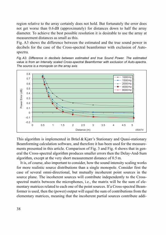
region relative to the array certainly does not hold. But fortunately the error doesnot get worse than 0.6 dB (approximately) for distances down to half the arraydiameter. To achieve the best possible resolution it is desirable to use the array atmeasurement distances as small as this.Fig. A3 shows the difference between the estimated and the true sound power indecibels for the case of the Cross-spectral beamformer with exclusion of Auto-spectra.

This algorithm is implemented in Brüel & Kjær�s Stationary and Quasi-stationaryBeamforming calculation software, and therefore it has been used for the measure-ments presented in this article. Comparison of Fig. 3 and Fig. 4 shows that in gen-eral the Cross-spectral algorithm produces smaller errors then the Delay-And-Sumalgorithm, except at the very short measurement distance of 0.5 m.

It is, of course, also important to consider, how the sound intensity scaling worksfor more realistic source distributions than a single monopole. Consider first thecase of several omni-directional, but mutually incoherent point sources in thesource plane. The incoherent sources will contribute independently to the Cross-spectral matrix between the microphones, i.e., the matrix will be the sum of ele-mentary matrices related to each one of the point sources. If a Cross-spectral Beam-former is used, then the (power) output will equal the sum of contributions from theelementary matrices, meaning that the incoherent partial sources contribute addi-

Fig. A3. Difference in decibels between estimated and true Sound Power. The estimatedvalue is from an Intensity scaled Cross-spectral Beamformer with exclusion of Auto-spectra.The source is a monopole on the array axis

1000 Hz

1500 Hz

2000 Hz

4000 Hz

8000 Hz

0 0.5 1 1.5 2 2.5 3 3.5 4 4.5 5

0.3

0.4

0.5

0.6

0.7

0.8

0.2

0.1

0

-0.1

-0.2

050074Distance (m)

Pow

er

Err

or

(dB

)

38

tively to the Beamformer (power) output. Since they contribute also additively tothe Sound Power, the conclusion is that the intensity scaling will hold for a set ofincoherent monopole point sources.When there is full or partial coherence between a set of monopole sources, theradiation from the total set of sources is no longer omni-directional, which willintroduce an error that cannot be compensated: The array covers only a certainpart of the 2π solid angle for which the sound power is desired. For angles not cov-ered by the array we do not know the radiation and therefore we cannot know thesound power.

References[1] Christensen J.J., Hald J., �Beamforming�, Brüel & Kjær Technical Review,

No. 1 (2004).

[2] Williams E.G., �Fourier Acoustics � Sound Radiation and Nearfield Acous-tical Holography�, Academic Press (1999).

[3] Hald J., �Patch Near-field Acoustical Holography using a New StatisticallyOptimal Method�, Proceedings of Inter-noise 2003.

[4] Hald J., Christensen J.J., �A Class of Optimal Broadband Phased ArrayGeometries designed for Easy Construction�, Proceedings of Inter-noise2002.

[5] Nordborg A., Wedemann J., Willenbrink L., �Optimum Array MicrophoneConfiguration�, Proceedings of Inter-noise 2000.

[6] Boeringer D.W., �Phased Array including a Logarithmic Lattice of Uni-formly Spaced Radiating and Receiving Elements�, United States PatentUS 6,433,754 B1.

[7] Unser M., �Sampling � 50 Years After Shannon�, Proceedings of the IEEE,Vol. 88, No. 4, April 2000.

[8] Oerlemans S., Sijtsma P., �Determination of Absolute Levels from PhasedArray Measurements Using Spatial Source Coherence�, AIAA 2002-2464.

[9] Johnson D. H., Dudgeon D. E., �Array Signal Processing: Concepts andTechniques�, Prentice Hall, New Jersey (1993).

39

Patch Near�field Acoustical Holography Using a New Statistically Optimal Method

J. Hald

AbstractThe spatial FFT processing used in Near-field Acoustical Holography (NAH)makes the method computationally efficient, but it introduces severe spatial win-dowing effects, unless the measurement area is significantly larger than the source.A Statistically Optimal NAH (SONAH) method is introduced which performs theplane-to-plane calculations directly in the spatial domain. Therefore, the need for arepresentation in the spatial frequency domain and for zero padding is avoided,significantly reducing the spatial windowing effects. This article describes theSONAH algorithm and presents some results from numerical simulations andpractical measurements.

RésuméLe traitement FFT spatial utilisé dans l�holographie acoustique en champ proche(NAH) rend la méthode efficace sur le plan computationnel mais s�accompagned�effets de fenêtrage inopportuns, sauf dans le cas où la surface mesurée est signifi-cativement plus grande que la source. La méthode faisant intervenir l�algorithmeStatistically Optimal NAH (SONAH) est ici présentée. Les calculs étant effectuésplan à plan dans le domaine spatial, elle évite le besoin d�une représentation dans ledomaine de fréquence spatial et d�un calage du zéro, réduisant de manière signifi-cative les effets de fenêtrage spatial. Cet article décrit l�algorithme SONAH et pré-sente plusieurs résultats obtenus par simulation numérique et par mesurespratiques.

ZusammenfassungDie bei der akustischen Nahfeldholographie (NAH) verwendete räumliche FFTmacht die Methode rechnerisch effizient, führt jedoch andererseits zu einem be-trächtlichen räumlichen Fenstereffekt, sofern die Messfläche nicht wesentlich grö-ßer ist als die Quelle.

40

Es wird eine statistisch optimierte Methode der akustischen Nahfeldholographie(SONAH) vorgestellt, die Berechnungen von Ebene zu Ebene direkt im räumlichenBereich ausführt. Damit entfällt die Notwendigkeit für eine Darstellung im räumli-chen Frequenzbereich und für Zero Padding, wodurch räumliche Fenstereffektewesentlich reduziert werden. Dieser Artikel beschreibt den SONAH Algorithmusund stellt Ergebnisse numerischer Simulationen und praktischer Messungen vor.

IntroductionA plane-to-plane propagation of a sound field away from the source can be

described mathematically as a 2D spatial convolution with a propagation kernel. A2D spatial Fourier transform reduces this convolution to a simple multiplication bya transfer function. In Near-field Acoustical Holography (NAH) the Fourier trans-form is implemented as a spatial FFT of the pressure data measured over a finitearea.

The use of spatial FFT and multiplication with a transfer function in the spatialfrequency domain is computationally very efficient, but it introduces some errors.The discrete representation in the spatial frequency domain introduces periodicreplica in the spatial domain, causing �wrap-around errors� in the calculationplane. A standard way of spacing the replica away from the real measurement areais to use zero padding, introducing, however, a sharp spatial window. Such a win-dow causes spectral leakage in the spatial frequency domain [1]. As a consequence,the measurement area must be significantly larger than the source to avoid very dis-turbing window effects. This is a problem, for example, in connection with TimeDomain NAH, [2], and Real-time NAH, which do not allow the synthesis of a largemeasurement area through scanning. The new Statistically Optimal NAH(SONAH) method performs the plane-to-plane transformation directly in the spa-tial domain rather than going via the spatial frequency domain, [3].

Theory of SONAHThe derivation of the SONAH algorithm given in this section is an extension ofthe derivation given in reference [4]. It is different from, and probably simplerthan, the one given in reference [3].

We consider a complex, time-harmonic sound pressure field p(r) = p(x, y, z) withfrequency f and wave number k = x/c = 2p/k where x = 2pf is the angular fre-quency, c is the propagation speed of sound and k is the wavelength. For the fol-lowing description we shall assume that the half space z ≥ �d is source free and

41

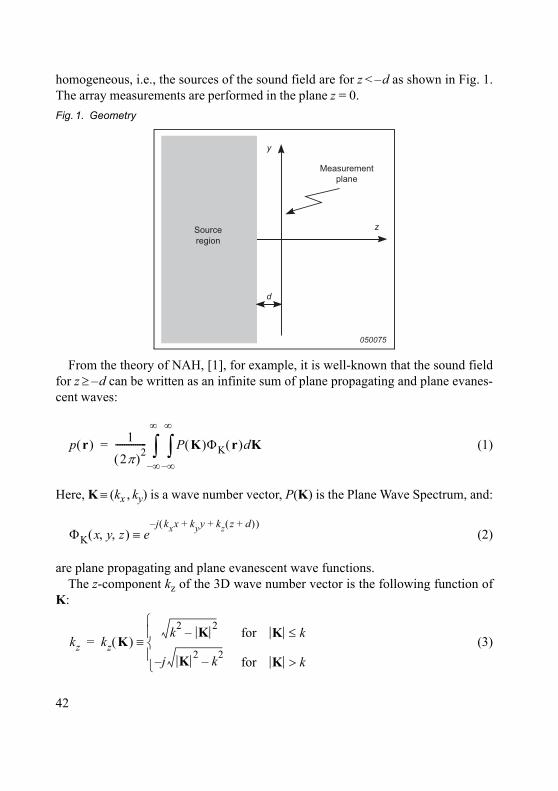
homogeneous, i.e., the sources of the sound field are for z < �d as shown in Fig. 1.The array measurements are performed in the plane z = 0.

From the theory of NAH, [1], for example, it is well-known that the sound fieldfor z ≥ �d can be written as an infinite sum of plane propagating and plane evanes-cent waves:

(1)

Here, K ≡ (kx , ky) is a wave number vector, P(K) is the Plane Wave Spectrum, and:

(2)

are plane propagating and plane evanescent wave functions. The z-component kz of the 3D wave number vector is the following function of

K:

(3)

Fig. 1. Geometry

Measurement

plane

y

z

d

Source

region

050075

p r( ) 1

2π( )2-------------- P

∞�

∞

∫∞�

∞

∫ K( )ΦK r( )dK=

ΦK x y z, ,( ) ej kxx kyy kz z d+( )+ +( )�

≡

kz kz K( )k2 K 2�

j� K 2 k2�⎩⎪⎨⎪⎧

≡=for K k≤

for K k>

42

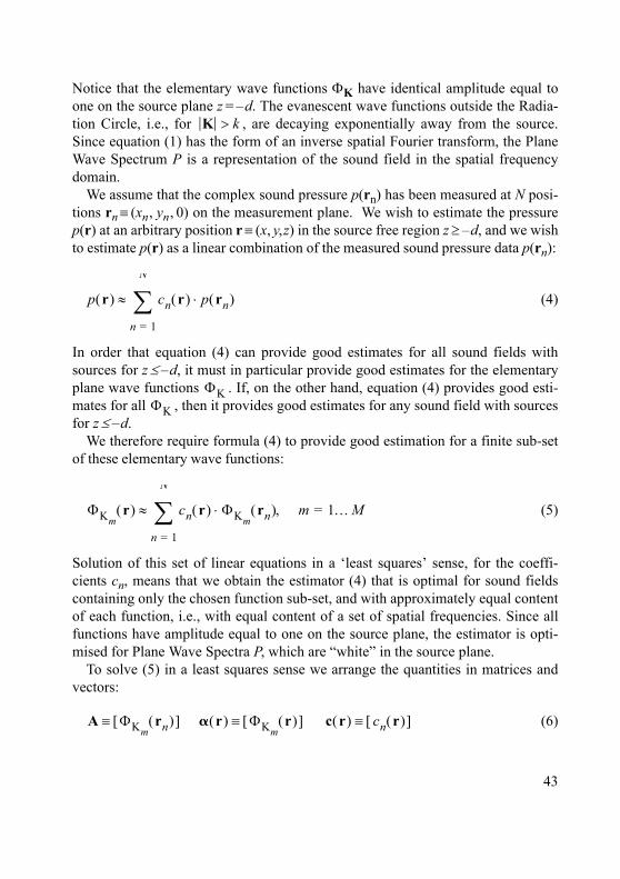
Notice that the elementary wave functions ΦK have identical amplitude equal toone on the source plane z = �d. The evanescent wave functions outside the Radia-tion Circle, i.e., for , are decaying exponentially away from the source.Since equation (1) has the form of an inverse spatial Fourier transform, the PlaneWave Spectrum P is a representation of the sound field in the spatial frequencydomain.

We assume that the complex sound pressure p(rn) has been measured at N posi-tions rn ≡ (xn, yn, 0) on the measurement plane. We wish to estimate the pressurep(r) at an arbitrary position r ≡ (x, y,z) in the source free region z ≥ �d, and we wishto estimate p(r) as a linear combination of the measured sound pressure data p(rn):

(4)

In order that equation (4) can provide good estimates for all sound fields withsources for z ≤ �d, it must in particular provide good estimates for the elementaryplane wave functions . If, on the other hand, equation (4) provides good esti-mates for all , then it provides good estimates for any sound field with sourcesfor z ≤ �d.

We therefore require formula (4) to provide good estimation for a finite sub-setof these elementary wave functions:

(5)

Solution of this set of linear equations in a �least squares� sense, for the coeffi-cients cn, means that we obtain the estimator (4) that is optimal for sound fieldscontaining only the chosen function sub-set, and with approximately equal contentof each function, i.e., with equal content of a set of spatial frequencies. Since allfunctions have amplitude equal to one on the source plane, the estimator is opti-mised for Plane Wave Spectra P, which are �white� in the source plane.

To solve (5) in a least squares sense we arrange the quantities in matrices andvectors:

(6)

K k>

p r( ) cn

n 1=

N

∑ r( ) p rn( )⋅≈

ΦKΦK

ΦKmr( ) cn

n 1=

N

∑ r( ) ΦKmrn( ) m 1…M=,⋅≈

A ΦKmrn( )[ ]≡ � r( ) ΦKm

r( )[ ]≡ c r( ) cn r( )[ ]≡

43

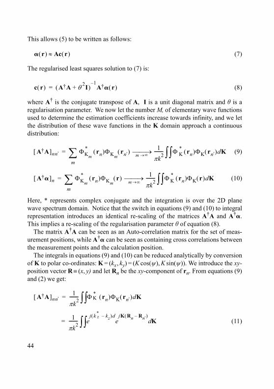
This allows (5) to be written as follows:

(7)

The regularised least squares solution to (7) is:

(8)

where A� is the conjugate transpose of A, I is a unit diagonal matrix and h is aregularisation parameter. We now let the number M, of elementary wave functionsused to determine the estimation coefficients increase towards infinity, and we letthe distribution of these wave functions in the K domain approach a continuousdistribution:

(9)

(10)

Here, * represents complex conjugate and the integration is over the 2D planewave spectrum domain. Notice that the switch in equations (9) and (10) to integralrepresentation introduces an identical re-scaling of the matrices A�A and A��.This implies a re-scaling of the regularisation parameter h of equation (8).

The matrix A�A can be seen as an Auto-correlation matrix for the set of meas-urement positions, while A�� can be seen as containing cross correlations betweenthe measurement points and the calculation position.

The integrals in equations (9) and (10) can be reduced analytically by conversionof K to polar co-ordinates: K = (kx, ky) = (K cos(w), K sin(w)). We introduce the xy-position vector R ≡ (x, y) and let Rn be the xy-component of rn. From equations (9)and (2) we get:

(11)

� r( ) Ac r( )≈

c r( ) A�A θ 2I+( )1�A�� r( )=

A�A[ ]nn' ΦKm

*

m∑ rn( )ΦKm

rn'( ) ⎯⎯→ 1

πk2-------- Φ K

*∫∫ rn( )ΦK rn'( )dK= m →∞

A��[ ]n ΦKm

*

m∑ rn( )ΦKm

r( ) ⎯⎯→ 1

πk2-------- Φ *

K∫∫ rn( )ΦK r( )dK=m →∞

A�A[ ]nn'1

πk2-------- Φ *

K∫∫ rn( )ΦK rn'( )dK=

1

πk2-------- e

j k *z kz�( )d

ejK Rn Rn'�( )

Kd∫∫=

44

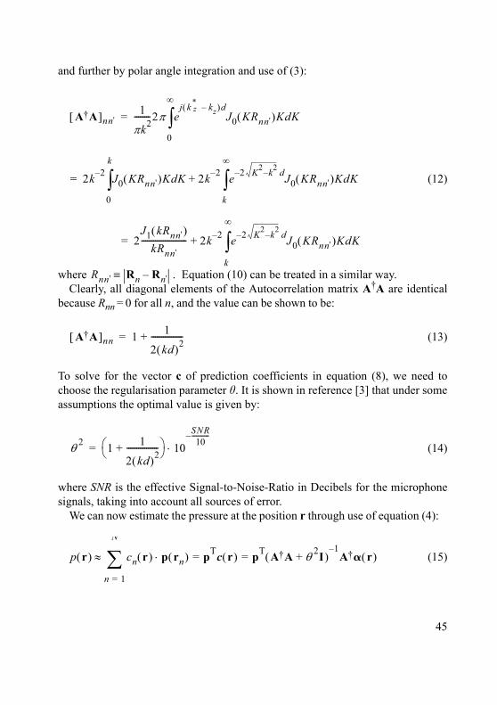
and further by polar angle integration and use of (3):

(12)

where . Equation (10) can be treated in a similar way.Clearly, all diagonal elements of the Autocorrelation matrix A�A are identical

because Rnn = 0 for all n, and the value can be shown to be:

(13)

To solve for the vector c of prediction coefficients in equation (8), we need tochoose the regularisation parameter h. It is shown in reference [3] that under someassumptions the optimal value is given by:

(14)

where SNR is the effective Signal-to-Noise-Ratio in Decibels for the microphonesignals, taking into account all sources of error.

We can now estimate the pressure at the position r through use of equation (4):

(15)

A�A[ ]nn'1

πk2--------2π e

j k *z kz�( )d

0

∞

∫ J0 KRnn'( )KdK=

2k 2� J0

0

k

∫ KRnn'( )KdK 2+ k 2� e 2 K2 k2�� dJ0

k

∞

∫ KRnn'( )KdK=

2J1 kRnn'( )

kRnn'----------------------- 2k 2� e 2 K2 k2�� d

k

∞

∫ J0 KRnn'( )KdK+=

Rnn' Rn Rn'�≡

A�A[ ]nn 1 1

2 kd( )2----------------+=

θ 2 1 1

2 kd( )2----------------+⎝ ⎠

⎛ ⎞ 10SNR10

-----------�⋅=

p r( ) cn

n 1=

N

∑ r( ) p rn( ) pTc r( ) pT A�A θ 2I+( )1�A�� r( )= =⋅≈

45

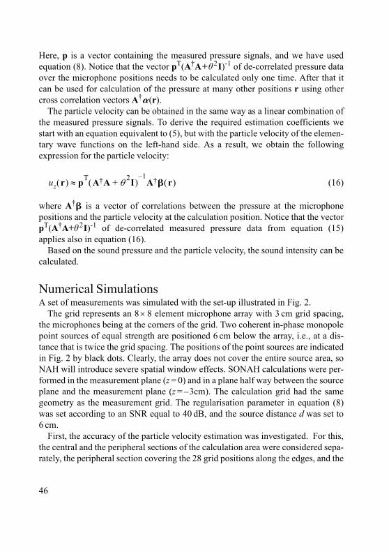
Here, p is a vector containing the measured pressure signals, and we have usedequation (8). Notice that the vector pT(A�A+h2I)-1 of de-correlated pressure dataover the microphone positions needs to be calculated only one time. After that itcan be used for calculation of the pressure at many other positions r using othercross correlation vectors A��(r).

The particle velocity can be obtained in the same way as a linear combination ofthe measured pressure signals. To derive the required estimation coefficients westart with an equation equivalent to (5), but with the particle velocity of the elemen-tary wave functions on the left-hand side. As a result, we obtain the followingexpression for the particle velocity:

(16)

where A�� is a vector of correlations between the pressure at the microphonepositions and the particle velocity at the calculation position. Notice that the vectorpT(A�A+h2I)-1 of de-correlated measured pressure data from equation (15)applies also in equation (16).

Based on the sound pressure and the particle velocity, the sound intensity can becalculated.

Numerical SimulationsA set of measurements was simulated with the set-up illustrated in Fig. 2.

The grid represents an 8 × 8 element microphone array with 3 cm grid spacing,the microphones being at the corners of the grid. Two coherent in-phase monopolepoint sources of equal strength are positioned 6 cm below the array, i.e., at a dis-tance that is twice the grid spacing. The positions of the point sources are indicatedin Fig. 2 by black dots. Clearly, the array does not cover the entire source area, soNAH will introduce severe spatial window effects. SONAH calculations were per-formed in the measurement plane (z = 0) and in a plane half way between the sourceplane and the measurement plane (z = �3cm). The calculation grid had the samegeometry as the measurement grid. The regularisation parameter in equation (8)was set according to an SNR equal to 40 dB, and the source distance d was set to6 cm.

First, the accuracy of the particle velocity estimation was investigated. For this,the central and the peripheral sections of the calculation area were considered sepa-rately, the peripheral section covering the 28 grid positions along the edges, and the

uz r( ) pT A�A θ 2I+( )1�A�� r( )≈

46

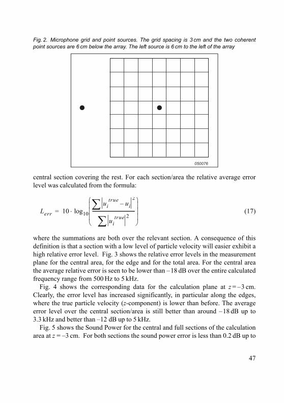
central section covering the rest. For each section/area the relative average errorlevel was calculated from the formula:

(17)

where the summations are both over the relevant section. A consequence of thisdefinition is that a section with a low level of particle velocity will easier exhibit ahigh relative error level. Fig. 3 shows the relative error levels in the measurementplane for the central area, for the edge and for the total area. For the central areathe average relative error is seen to be lower than �18 dB over the entire calculatedfrequency range from 500 Hz to 5 kHz.

Fig. 4 shows the corresponding data for the calculation plane at z = �3 cm.Clearly, the error level has increased significantly, in particular along the edges,where the true particle velocity (z-component) is lower than before. The averageerror level over the central section/area is still better than around �18 dB up to3.3 kHz and better than �12 dB up to 5 kHz.

Fig. 5 shows the Sound Power for the central and full sections of the calculationarea at z = �3 cm. For both sections the sound power error is less than 0.2 dB up to

Fig. 2. Microphone grid and point sources. The grid spacing is 3 cm and the two coherentpoint sources are 6 cm below the array. The left source is 6 cm to the left of the array

050076

Lerr 10 log10

uitrue ui�

2∑

uitrue 2∑

--------------------------------------

⎝ ⎠⎜ ⎟⎜ ⎟⎜ ⎟⎛ ⎞

⋅=

47

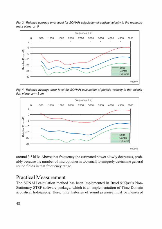
around 3.5 kHz. Above that frequency the estimated power slowly decreases, prob-ably because the number of microphones is too small to uniquely determine generalsound fields in that frequency range.

Practical MeasurementThe SONAH calculation method has been implemented in Brüel & Kjær�s Non-Stationary STSF software package, which is an implementation of Time Domainacoustical holography. Here, time histories of sound pressure must be measured

Fig. 3. Relative average error level for SONAH calculation of particle velocity in the measure-ment plane, z=0

Fig. 4. Relative average error level for SONAH calculation of particle velocity in the calcula-tion plane, z= �3 cm

Edge

Center

Full area

0 500 1000 1500 2000 2500 3000 3500 4000 4500 5000

0

-5

-10

-15

-20

-25

-30

050077

Frequency (Hz)

Rela

tive E

rror

(dB

)

Edge

Center

Full area

0 500 1000 1500 2000 2500 3000 3500 4000 4500 5000

5

0

-5

-10

-15

-20

-25

050065

Frequency (Hz)

Rela

tive E

rror

(dB

)

48

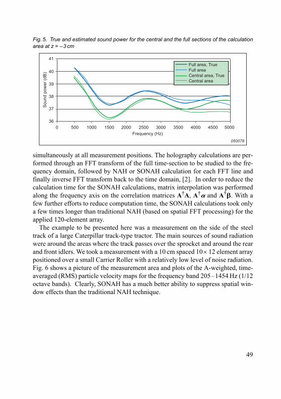
simultaneously at all measurement positions. The holography calculations are per-formed through an FFT transform of the full time-section to be studied to the fre-quency domain, followed by NAH or SONAH calculation for each FFT line andfinally inverse FFT transform back to the time domain, [2]. In order to reduce thecalculation time for the SONAH calculations, matrix interpolation was performedalong the frequency axis on the correlation matrices A�A, A�� and A��. With afew further efforts to reduce computation time, the SONAH calculations took onlya few times longer than traditional NAH (based on spatial FFT processing) for theapplied 120-element array.

The example to be presented here was a measurement on the side of the steeltrack of a large Caterpillar track-type tractor. The main sources of sound radiationwere around the areas where the track passes over the sprocket and around the rearand front idlers. We took a measurement with a 10 cm spaced 10 × 12 element arraypositioned over a small Carrier Roller with a relatively low level of noise radiation.Fig. 6 shows a picture of the measurement area and plots of the A-weighted, time-averaged (RMS) particle velocity maps for the frequency band 205�1454 Hz (1/12octave bands). Clearly, SONAH has a much better ability to suppress spatial win-dow effects than the traditional NAH technique.

Fig. 5. True and estimated sound power for the central and the full sections of the calculationarea at z = �3 cm

Full area, True

Full area

Central area, True

Central area

0 500 1000 1500 2000 2500 3000 3500 4000 4500 5000

41

40

39

38

37

36

050078

Frequency (Hz)

So

un

d p

ow

er

(dB

)

49

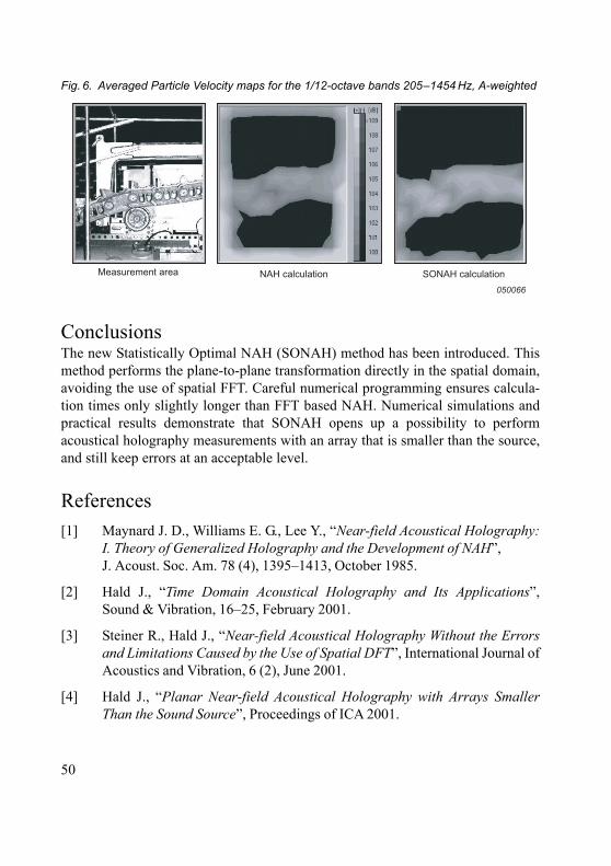
ConclusionsThe new Statistically Optimal NAH (SONAH) method has been introduced. Thismethod performs the plane-to-plane transformation directly in the spatial domain,avoiding the use of spatial FFT. Careful numerical programming ensures calcula-tion times only slightly longer than FFT based NAH. Numerical simulations andpractical results demonstrate that SONAH opens up a possibility to performacoustical holography measurements with an array that is smaller than the source,and still keep errors at an acceptable level.

References[1] Maynard J. D., Williams E. G., Lee Y., �Near-field Acoustical Holography:

I. Theory of Generalized Holography and the Development of NAH�, J. Acoust. Soc. Am. 78 (4), 1395�1413, October 1985.

[2] Hald J., �Time Domain Acoustical Holography and Its Applications�,Sound & Vibration, 16�25, February 2001.

[3] Steiner R., Hald J., �Near-field Acoustical Holography Without the Errorsand Limitations Caused by the Use of Spatial DFT�, International Journal ofAcoustics and Vibration, 6 (2), June 2001.

[4] Hald J., �Planar Near-field Acoustical Holography with Arrays SmallerThan the Sound Source�, Proceedings of ICA 2001.

Fig. 6. Averaged Particle Velocity maps for the 1/12-octave bands 205�1454 Hz, A-weighted

SONAH calculationNAH calculation

050066

Measurement area

50

1 � 1989 STSF � A Unique Technique for Scan Based Near-Field Acoustic Holography Without Restrictions on Coherence

2 � 1988 Quantifying Draught Risk1 � 1988 Using Experimental Modal Analysis to Simulate Structural Dynamic

ModificationsUse of Operational Deflection Shapes for Noise Control of Discrete Tones

4 � 1987 Windows to FFT Analysis (Part II)Acoustic Calibrator for Intensity Measurement Systems

3 � 1987 Windows to FFT Analysis (Part I)2 � 1987 Recent Developments in Accelerometer Design

Trends in Accelerometer Calibration1 � 1987 Vibration Monitoring of Machines4 � 1986 Field Measurements of Sound Insulation with a Battery-Operated Intensity

AnalyzerPressure Microphones for Intensity Measurements with Significantly Improved Phase PropertiesMeasurement of Acoustical Distance between Intensity Probe MicrophonesWind and Turbulence Noise of Turbulence Screen, Nose Cone and Sound Intensity Probe with Wind Screen

3 � 1986 A Method of Determining the Modal Frequencies of Structures with Coupled ModesImprovement to Monoreference Modal Data by Adding an Oblique Degree of Freedom for the Reference

2 � 1986 Quality in Spectral Match of Photometric TransducersGuide to Lighting of Urban Areas

1 � 1986 Environmental Noise Measurements

Special technical literatureBrüel & Kjær publishes a variety of technical literature which can be obtained from your local Brüel & Kjær representative.

The following literature is presently available:

� Catalogues (several languages)� Product Data Sheets (English, German, French,)

Furthermore, back copies of the Technical Review can be supplied as listed above. Older issues may be obtained provided they are still in stock.

Previously issued numbers ofBrüel & Kjær Technical Review(Continued from cover page 2)

HEADQUARTERS: DK-2850 Nærum · DenmarkTelephone: +45 45 80 05 00 · Fax: +45 45 80 14 05www.bksv.com · [email protected]

BV

0057

–11

ISSN

000

7–26

21

BV0070-11_TR_Cover2005.qxp 21-03-2005 13:29 Page 1