Technical Report TR-UA-ECE-2008-4 August 2008

Throughput-optimal Sequential Channel Sensingand Probing in Cognitive Radio Networks

Tao Shu and Marwan KrunzDepartment of Electrical and Computer Engineering

University of Arizona

Technical ReportTR-UA-ECE-2008-4

August 2008

AbstractIn a dynamic spectrum sharing system, a cognitive radio (CR) is provided with more

channels than what it can use. So it is important for the CR to select the right channelsfor its transmission. To avoid interfering with incumbent primary radios, the existingschemes are based on channel sensing, which use the busy/idle status of a channel asthe criterion to select channels. Such schemes in general do not provide good throughputperformance for CRs. In this paper, we study a throughput-optimal joint sensing/probingscheme for CRs that uses the channel quality as a second criterion in selecting channels.The difficulty of this problem comes from the fact that a CR cannot first scan all channelsand then pick the best one. This is because the total number of channels might belarge, while a CR senses and probes channels sequentially due to its power and hardwarelimitations. After sensing and probing a channel, the CR needs to make a decision aboutwhether to terminate the scan and use the underlying channel or to skip it and scan thenext one. The optimal use-or-skip decision strategy that maximizes the CR’s averagethroughput is one of our primary concerns in this study. This optimal strategy is derivedby formulating the above sequential channel sensing/probing/access process as an infinite-horizon rate-of-return problem, which we solve using optimal stopping theory. We thenfurther look into the structure of this strategy to conduct a second-round optimizationover the operational parameters, such as the sensing and probing times. We show throughnumerical examples that when these operational parameters are properly set, significantthroughput gain (e.g., about 100%) can be achieved by our joint sensing/probing schemeover the conventional one that uses sensing alone.

1 Introduction

The benefit of dynamic spectrum sharing (DSS) as a means of improving spectrum utilization

is now well recognized [18]. DSS aims at opening the under-utilized portions of the spectrum

1

for secondary re-use, provided that the transmissions of secondary radios do not cause harmful

interference to the licensed radios (a.k.a., primary radios (PRs)). Because now a secondary

radio is provided with more channels than what it can use, a critical challenge in DSS is to

select in real-time the channels that the secondary radios should use. Such a selection should

provide a secondary radio with the maximum possible throughput under the premise that PRs

will not be negatively affected by this selection. For scalability purposes, a distributed selection

algorithm is also desirable.

The cognitive radio (CR) is regarded as the enabling technology for DSS [13]. The conven-

tional way for a CR to select channels distributedly is to scan (sense) channels and access those

channels that are deemed to be idle. Although this approach guarantees a safe (secondary)

access to spectrum for CRs, it generally does not give optimal throughput performance. This is

because the CR does not account for the quality of the idle channel. As a result, transmitting

over channels of poor conditions comprises the CR’s throughput.

In this paper, we study a joint sensing/probing mechanism for cognitive radio networks

(CRNs) to improve the throughput. This mechanism uses the channel quality information as

a second criterion for channel selection. Specifically, a channel-probing component is added

right after channel sensing to decide the maximum data rate supported by the probed channel.

Among idle channels, a CR will use only good channels that support relatively high data rates.

Although the use of probing has been comprehensively studied in the past for general

wireless systems [14], the problem is new in the context of CRNs. First, unlike previous work,

channel selection in a CRN is sequential. Due to the large number of channels and the CR’s

power/hardware limitations, it is not possible for a CR to first scan all channels simultaneously

and then pick the best one. A CR can only sense and probe channels sequentially. After

sensing and probing a channel, the CR needs to decide whether to terminate the scan and use

the underlying channel or to skip it and scan the next one. Furthermore, to avoid collisions

with PRs, a CR cannot recall (use) a channel it previously skipped, because of the staleness

of that sensing outcome (the channel may have been taken by other CR or PR transmissions).

This non-recall use of channel along with the lack of knowledge about the conditions of those

un-probed channels make such a sequential decision making non-trivial. Second, the decision

making process becomes even more difficult when the CR’s sensing and probing overheads need

to be accounted for in each step. Empirical data shows that sensing one channel takes tens of ms

and probing one new channel takes from 10 to 133 ms, depending on the association and capture

2

speed between the transmitter and receiver after each channel hopping [1]. At the same time,

to reduce collisions with newly activated PRs, a CR’s transmission time over an idle channel

must be restricted, e.g., in the order of hundreds of ms or at most few seconds. Therefore, the

accumulated overhead after sequentially sensing/probing several channels becomes comparable

with or even greater than the CR’s transmission time. When these overheads are concerned,

to find a slightly better channel may not justify continuing the channel search process. As will

become clear shortly, these new aspects of a CRN require a totally new formulation for the

problem.

In this paper, we address the following key issues that are aimed at making the CRN’s

sensing/probing/access scheme operationally efficient. First, we derive the throughput-optimal

decision strategy for the sequential channel sensing/probing process. It turns out that this

optimal strategy has a threshold structure, which basically says whether the channel is good

or bad. To set this threshold properly, we need to consider the tradeoff between the achievable

data rate brought by good channels and the time cost (and consequently, throughput reduction)

for searching for good channels. Second, we derive the maximum acceptable channel probing

time that guarantees a positive throughput gain for the proposed method over a scheme that

does not utilize probing. This knowledge is important because the accumulated probing time

may be so significant that it cancels out gains achieved by selecting good channels. Third,

we optimize the channel sensing time. In realistic systems, this sensing time determines the

accuracy of the channel sensing process. A shorter sensing time reduces the scanning time of

each channel at the expense of increasing the sensing false alarm rate, making the CR miss

more spectrum opportunities. This in turn increases the number of channels the CR needs to

sense and probe, leading to possibly longer overall channel search time. We exploit the tradeoff

between the sensing time and sensing accuracy to minimize the total channel search time (or

equivalently, maximize the throughput). Our work is the first to incorporate the relationship

between the sensing time and sensing accuracy in a multi-rate setting.

The above contributions are achieved by performing two rounds of optimizations. In the

first round, we treat the sensing and probing times as parameters, and derive the parametric

optimal probing strategy. This is achieved by formulating the sensing/probing/access process as

an infinite-horizon maximum rate-of-return problem in the optimal stopping theory [3], with the

number of bits that the CR is able to send in one transmission as the return, and the overall

3

channel search plus transmission times as the time cost. Next, we look into the particular

structure of the optimal probing strategy and perform a second round of optimization over

the operational parameters, such as the sensing and probing times, aiming at maximizing the

outcome of the first-round optimization.

Besides the above optimization considerations, we are also interested in the aggregate

throughput performance when a network of CRs coexist with PRs, and each CR reacts ac-

cording to the sensing/probing/access scheme in a distributed way. A Markov-chain model

is developed for our performance analysis, whereby the contention between CRs, the sensing

strategies employed (random channel sensing and collaborative channel sensing), and probing

threshold settings at individual CRs are all accounted for. Our results show that when the

sensing/probing parameters are properly set, the addition of probing can significantly improve

the CRN’s throughput, e.g., over 100% gains are observed in our simulations.

The remainder of this paper is organized as follows. Section 2 describes the system model

and its maximum rate of return formulation. Based on optimal-stopping theory, we solve

the optimization problem in Section 3. Section 4 studies the performance for multi-CR case.

Numerical results are presented in Section 5. Section 6 reviews related works and Section 7

concludes the paper. All proofs of the theorems are given in the appendix.

2 Model Description and Problem Formulation

2.1 System Model

We consider a set of C licensed channels. The status of a channel is modeled as a continuous-

time random process that alternates between two states: IDLE and BUSY. A BUSY (IDLE)

state indicates that some (no) PR user is transmitting over the channel. Denote the average

IDLE and BUSY durations by α and β, respectively. When the channel is observed at an

arbitrary time, its idle and busy probabilities are given by PI = αα+β

and PB = βα+β

, respectively.

Here we focus on the homogeneous channel utilization scenario, i.e., we assume that the states

of different channels are driven by homogeneous and independent random process. This may

correspond to the scenario that all channels belong to the same licensed network. The channel

selection problem under heterogeneous channel utilization is actually trivial, because in that

case a CR should select the channel with the lowest utilization.

Along with the PR users, the spectrum is opportunistically shared with a number of CRs.

4

sτ pτ

tτ

Figure 1: Sequential channel sensing and probing before transmission.

To simplify the exposure, we ignore for the time being the CR-to-CR contention issue related to

having multiple CRs. This allows us to focus on the channel sensing/probing/access process of

a pair of CR transmitter and receiver, with the goal of optimizing this process. We also assume

that some synchronization mechanism (e.g., a random-number-generater-based one) is in place

so that the CR transmitter and receiver are always sensing and probing the same channel at the

same time. We will account for the contention issue in Section 4 when we study the multi-CR

scenario.

When a CR wants to transmit, it starts searching for channels sequentially, as shown in

Figure 1. Specifically, at the beginning, the CR randomly picks channel c1, 1 ≤ c1 ≤ C, and

samples it for τs time. Then the CR decides whether channel c1 is idle or busy. If it is busy,

the CR randomly selects the next channel c2, 1 ≤ c2 ≤ C, to sample, and so on. Suppose that

in the nth step, channel cn is determined as idle. Then the CR transmitter begins to probe

that channel by sending a channel probing packet (CPP) over channel cn using a predefined

power. The CR receiver measures the strength of the received CPP and decides the maximum

achievable data rate (MADR), rn, that can be supported by the current channel. The value

of rn is selected from a set of discrete rates: {Rk, k = 0, 1, . . . , K}, where Rk increases with

k and R0 = 0. This MADR value is then embedded into a probing feedback packet (PFP),

which is sent back from the receiver to the transmitter over channel cn. The time spent

on one CPP/PFP exchange plus the preceding time for association and capture between the

transmitter and receiver is called the channel probing time τp. After receiving the PFP, the

transmitter decides whether to use this channel or not. This is done by comparing rn with some

channel quality threshold, r∗. If rn ≥ r∗, then the transmitter terminates the channel search

and transmits at rate rn over channel cn for τt duration of time (τt should be short enough such

that collisions with newly activated PRs for this amount of time are deemed acceptable). If

rn < r∗, the CR will skip this channel and continue to sense the next one. Because the CR

5

receiver also has knowledge of r∗ (e.g., this information can be embedded into the CPP), there

is no need for the transmitter to notify the receiver about its decision. Note that if the channel

is busy during the sensing phase, no probing packets should be exchanged between the CR

transmitter and receiver, to avoid interfering with PRs. However, the receiver still has to wait

for τp time to realize that the channel must be busy. Therefore, whether or not the channel is

idle, the time cost for one step of channel search is τs + τp.

Remark: If a CR can transmit over J idle channels at a time, then J parallel channel search-

ing/access instances can be initiated and maintained by the CR. Each instance will indepen-

dently search and use one idle channel according to the above sequential process. The opti-

mizations over each instance are identical and independent. Therefore we only need to focus

on one such instance in our treatment.

Channel sensing is modeled as a binary hypothesis test, where H0 indicates an idle channel

and H1 indicates an occupied channel. Let x(t) be the sample collected by the CR. Then,

x(t) =

{n(t), H0 (idle)s(t) + n(t), H1 (occupied)

(1)

where n(t) is the AWGN and s(t) is the received PR’s signal at the CR. Regarding this sensing

process, the probabilities of false alarm Pfa and miss detection Pmd are defined as follows

Pfa(τs) = Pr{CR decides the channel is busy|H0} (2)

Pmd(τs) = Pr{CR decides the channel is idle|H1}. (3)

Note that these two probabilities are functions of the sensing time τs.

The unconditional probabilities that a CR decides a channel is idle (QI) or busy (QB) are

given by

QI = PBPmd + PI(1− Pfa) ≈ PI(1− Pfa) (4)

QB = PB(1− Pmd) + PIPfa ≈ PB + PIPfa (5)

The approximation in the last steps is due to the practical requirement that Pmd ¿ 1 (e.g., 1%

is a typical value), which ensures a secondary role for the CRs.

2.2 Problem Formulation

The throughput-optimal sequential channel sensing/probing/access process can be formulated

as an optimal stopping problem. We first briefly describe the definition of an optimal stopping

problem and then present our formulation.

6

An optimal stopping problem is defined by the following two components [3]:

1. A sequence of random variables X1, X2, . . . , whose joint distribution is assumed to be

known.

2. A sequence of real-valued reward functions, y0, y1(x1), y2(x1, x2), . . . , y∞(x1, x2, . . .).

The sequence X1, X2, . . ., can be observed sequentially (one variable at a time) for as long as

needed. For each observation instance n = 1, 2, . . . , after observing X1 = x1, X2 = x2, . . . , Xn =

xn, one may stop and receive the known reward yn(x1, . . . , xn), or one may continue to observe

Xn+1. If the decision is not to take any observations, the received reward is the constant y0. If

the observer never stops, the received reward is y∞(x1, . . . , ). The goal is to choose a rule to

stop such that the expected reward at the stopping time N , E{yN}, is maximized. According

to this framework, the optimal-stopping formulation of our problem is as follows.

First, we define the sequence of observations. For the nth sensing and probing step, n ≥ 1,

the MADR value of the channel, rn ∈ {0, R1, . . . , RK}, can be obtained. Depending on the

fading and shadowing effects on the channel, let the distribution of rn be pk = Pr{rn = Rk},k = 0, 1, . . . , K (we assume the fluctuations on different channels are i.i.d.). We define Xn as

the outcome of the nth-step sensing and probing: Xn = 0 if the channel is busy and Xn = rn

if the channel is idle. The distribution of Xn can be calculated as follows.

q0def= Pr{Xn = 0} = QB + QIp0 (6)

qkdef= Pr{Xn = Rk} = QIpk, for 1 ≤ k ≤ K. (7)

Next, we define the sequence of rewards: The reward of stopping after observing Xn is

defined as the throughput achieved by transmitting over channel cn and with the entire time

span (i.e., from the beginning of observing X1 until the end of transmission over channel cn)

taken into account. Recall that the use of channel must be non-recall. Mathematically, the

reward for transmitting over channel cn is given by

yn(X1, . . . , Xn)def= yn(Xn) =

Beff (n)

Ttot(n)=

Xnτt(1− Ploss)

n(τs + τp) + τt

(8)

where Beff (n) is the number of collision-free data bits that can be transmitted over channel cn,

Ttot(n) is the total time cost including channel search and transmission times, and Ploss is the

7

probability that channel cn is re-occupied by some returning PR during the CR’s transmission,

and thus a collision occurs and the CR’s transmission is void. Defining the moment of sensing

as the reference point, denote the forward recurrence time of the channel’s IDLE period by the

random variable τ̃0 and its pdf by f̃0. We can calculate Ploss as follows

Ploss = Pr{τ̃0 < τt} =

∫ τt

0

f̃0(t)dt. (9)

Following standard renewal theory analysis:

f̃0(t) =1− ∫ t

0 f0(τ)dτ∫∞0 τf0(τ)dτ

(10)

where f0 is the pdf of the channel’s IDLE period. For example, if f0 is an exponential

distribution with mean α, then f̃0 = f0 and Ploss can be calculated as Ploss = 1− e−τtα .

Define Ψ = {N : N ≥ 1, E[Ttot(N)] < ∞} as the set of all possible stopping rules. Our

problem is to find an optimal stopping rule N∗ ∈ Ψ that maximizes the following rate-of-return

objective function:

maximizeN∈ΨE{Beff (N)}E{Ttot(N)} . (11)

Clearly, because the CR decides after each observation whether or not to stop (according to

some rule), the final stopping time N becomes a random variable. Therefore, the number of

bits that can be effectively transmitted at the stopping point, Beff (N), together with the time

cost Ttot(N), are both random variables related to N . This is in contrast to the Beff (n) and

Ttot(n) in (8), where n is a constant.

The reason we wish to maximize the ratio in (11) rather than the true expected average

E{

Beff (N)

Ttot(N)

}is that if the problem is repeated independently Z times with a fixed stopping rule

leading to i.i.d. stopping times, N1, . . . , NZ and i.i.d. returns Beff (N1), . . . , Beff (NZ), then

the overall average return per unit time is the ratio (Beff (N1) + . . . + Beff (NZ))/(Ttot(N1) +

. . . + Ttot(NZ)). As Z → ∞, the limit of the expectation of the above ratio (if it exists) must

converge to E{Beff (N)}/E{Ttot(N)} by the law of large numbers [3]. Therefore, our objective

function can be interpreted as the long-term average throughput provided by the stopping rule.

3 Optimal Stopping Rule and Optimization Considera-

tions

In this section, we first solve the maximum-rate-of-return problem (11) using optimal stopping

theory. We then further examine the structure of our solution to address the optimization

8

issues raised in Section 1.

3.1 Throughput-optimal Stopping Rule

The solution to (11) heavily hinges on the optimal stopping theory [3]. Specifically, according

to [3], in order to solve problem (11), we can first consider a transformed version of the problem,

whose reward sequence is defined by

wn = Beff (n)− λTtot(n)

= Xnτt(1− Ploss)− λ[n(τs + τp) + τt]. (12)

When the parameter λ is chosen such that the optimal expected reward of the transformed

problem, i.e., V ∗ def= supN∈ΨE{Beff (N)−λTtot(N)}, becomes zero, the optimal stopping rule N∗

of this transformed problem is also the optimal stopping rule of the original problem (11). In

addition, the solution of λ that makes V ∗ = 0 hold, denoted as λ∗, is the maximum throughput

in (11) achieved by the optimal stopping rule N∗. Applying this philosophy, we present the

following results regarding the existence and solution of the optimal stopping rule for problem

(11).

Theorem 1: An optimal solution to (11) exists. The maximum throughput λ∗ that is achieved

by this optimal stopping rule is the solution of the equation: E{max(Xnτt(1−Ploss)−λ∗τt, 0)} =

λ∗(τs + τp). The optimal stopping rule is given by N∗ = min{n ≥ 1 : Xn ≥ λ∗1−Ploss

}.All proofs of theorems are presented in Appendix. Regarding the calculation of the optimal

throughput and the optimal stopping rule of (11), we have the following theorem:

Theorem 2: λ∗ has a unique solution.

For the particular discrete-rate CRs considered in our work, a fast numerical algorithm can

be developed to calculate the exact λ∗ in at most O(K) time, where K is the number of rates

supported by the CR. Such an algorithm is based on the following observations. First, for the

multi-rate system Xn ∈ (R0, R1, . . . , RK), where R0 = 0 < R1 < . . . < RK , define k∗ to be the

minimum integer that satisfies Rk∗ ≥ λ∗1−Ploss

. Obviously, 1 ≤ k∗ ≤ K. Using this notation, the

equation E{max(Xnτt(1− Ploss)− λ∗τt, 0)} = λ∗(τs + τp) can be written as

g(λ∗) def=

K∑

k=k∗(Rkτt(1− Ploss)− λ∗τt)qk = λ∗(τs + τp),

given that Rk∗−1 <λ∗

1− Ploss

≤ Rk∗ . (13)

9

This gives a candidate solution for λ∗

λ∗ =τt(1− Ploss)

∑Kk=k∗ Rkqk

τs + τp + τt∑K

k=k∗ qk

, if Rk∗−1 <λ∗

1− Ploss≤ Rk∗ (14)

The range of values for k∗ is from 1 to K. Therefore, one can first enumerate all candidates of

λ∗ according to (14), and then pick the one that satisfies the condition Rk∗−1 < λ∗1−Ploss

≤ Rk∗ .

Theorem 2 guarantees that there is only one candidate satisfying this condition. The particular

Rk∗ under which the right λ∗ is obtained is the threshold rule that determines whether an idle

channel is good enough to be used.

3.2 Optimization Considerations

3.2.1 Impact of Probing Overhead

In this section, we evaluate the relationship between λ∗ and the operational parameters τs and

τp. We first look into the structure of the optimal solution (14). It turns out that λ∗ can be

written as a segmented function. Specifically, for the jth segment, 1 ≤ j ≤ K, the value of λ∗

satisfies Rj−1(1 − Ploss) < λ∗ ≤ Rj(1 − Ploss). To satisfy this condition, it must be the case

that

Rj−1 <τt

∑Kk=j Rkqk

τs + τp + τt

∑Kk=j qk

≤ Rj. (15)

After some mathematical manipulations, (15) leads to the following condition:

∑Kk=j Rkqk −Rj

∑Kk=j qk

Rj

≤ τs + τp

τt

<

∑Kk=j Rkqk −Rj−1

∑Kk=j qk

Rj−1

. (16)

The ratio ηdef= τs+τp

τtrepresents the efficiency of the channel sensing/probing/access scheme.

All the time factors in (16) are separated from the upper and lower bounds of the segment,

allowing a neat partition of segments based on η. Following this thread, λ∗ can be explicitly

written in the following segmented form:

λ∗ =

λ∗1(η) for φ1 ≤ η < Φ1...λ∗j(η) for φj ≤ η < Φj...λ∗K(η) for φK ≤ η < ΦK

(17)

where λ∗j(η)def=

(1−Ploss)∑K

k=j Rkqk

η+∑K

k=j qk, φj

def=

∑Kk=j Rkqk−Rj

∑Kk=j qk

Rj, and Φj

def=

∑Kk=j Rkqk−Rj−1

∑Kk=j qk

Rj−1,

j = 1, . . . , K. Because we are interested in determining whether the inclusion of probing leads

10

to better performance, we can assume τs and τt to be fixed (we will discuss the case when τs is

an optimization variable shortly), and analyze the structure of λ∗ as a function of τp. In this

sense, η becomes a one-to-one image of τp.

Theorem 3: Given τs and τt, the function λ∗ defined in (17) is a continuous and strictly

mono-decreasing segmented function over the entire domain of η.

When probing is not used, the average throughput, denoted by λ′, can be derived as follows.

First, the number of channels that are sensed until an idle channel is found follows a geometric

distribution with parameter QI . So the average time cost for finding an idle channel is given

by Tsdef= τs/QI . Once an idle channel is found, the average data rate supported by that channel

is R̄ =∑K

k=1 Rkpk. So λ′ is calculated as

λ′ =(1− Ploss)τt

∑Kk=1 Rkpk

Ts + τt

=(1− Ploss)

∑Kk=1 Rkqk

η′ + QI

(18)

where η′ def= τs

τt. Given τs and τt, λ′ is a constant. The equation λ∗(η) = λ′ must have a unique

solution. This is because when τt = 0, the sensing/probing/access scheme is at least as good

as the sensing/access scheme, while τt →∞, λ∗(∞) = 0 < λ′. The property presented in The-

orem 3 guarantees the existence of a unique intersection between λ∗(η) and λ′. Therefore, the

maximum acceptable τt that guarantees a throughput gain for sensing/probing/access scheme

is given by

τmaxp = τtλ

∗−1(λ′)− τs (19)

where λ∗−1(·) denotes the inverse function of λ∗(η). The significance of (19) is that it dictates

when probing should be used for a given set of sensing/probing/access parameters.

3.2.2 Impact of Sensing Time

In this section, we are interested in the impact of τs on the optimal throughput. It is well

known that for a given sensing/access CR system, throughput is a concave function of τs [11].

So there exists an optimal sensing time that maximizes the throughput. However, our finding

in this section reveals that in general the concavity of the throughput is not preserved when

probing is included, largely due to the more complicated structure of the multi-rate system.

The encouraging side of our finding is that when τs is the variable, the throughput maintains its

segmented structure. Treating a segment as our evaluation unit, the trend of the throughput

is concave over the segments of τs. Based on this property, we can derive a closed range Tos

that contains the optimal sensing time τ os . The value of this range is that for any τs ∈ To

s, it

11

leads to a throughput greater than what can be achieved under any τs /∈ Tos. The range To

s is

also provably efficient, i.e., any value inside this range can achieve at least a provable fraction

of the maximum throughput achieved with τ os . As a result, achieving provably near-optimal

performance is still guaranteed.

Our analysis involves evaluating the partition points of each segment defined in (17). In

total, there are K + 1 distinct partition points: φ0def= Φ1 = ∞ > φ1 > φ2 > . . . > φK−1 > φK =

0, where the new notation φ0 is defined for presentation convenience. For 1 ≤ j ≤ K − 1, φj

can be written as

φj = (1− Pfa(τs))Cj (20)

where Cjdef=

PI∑K

k=j(Rk−Rj)pk

Rjis a channel-dependent quantity that does not depend on τs.

We consider an energy detector for the channel sensing, for which the channel false alarm

probability is approximated by [11]

Pfa(τs) = Q

((ε

σ2u

− 1

) √τsfs

)(21)

where εσ2

uis the decision threshold for sensing and fs is the bandwidth of the channel. Given a

minimum sensing time τmins and a desired miss detection probability P̄md, the decision threshold

should be chosen such that for any τs ≥ τmins , we have Pmd(τs) ≤ P̄md, i.e., [11]

ε

σ2u

= Q−1(1− P̄md)√

2γ + 1τmins fs + γ + 1 (22)

where γ is the received signal-to-noise ratio of the PR signal at the CR. The relationship

between Pfa and τs in (21) is not in closed-form and thus is hard to manipulate. Given the

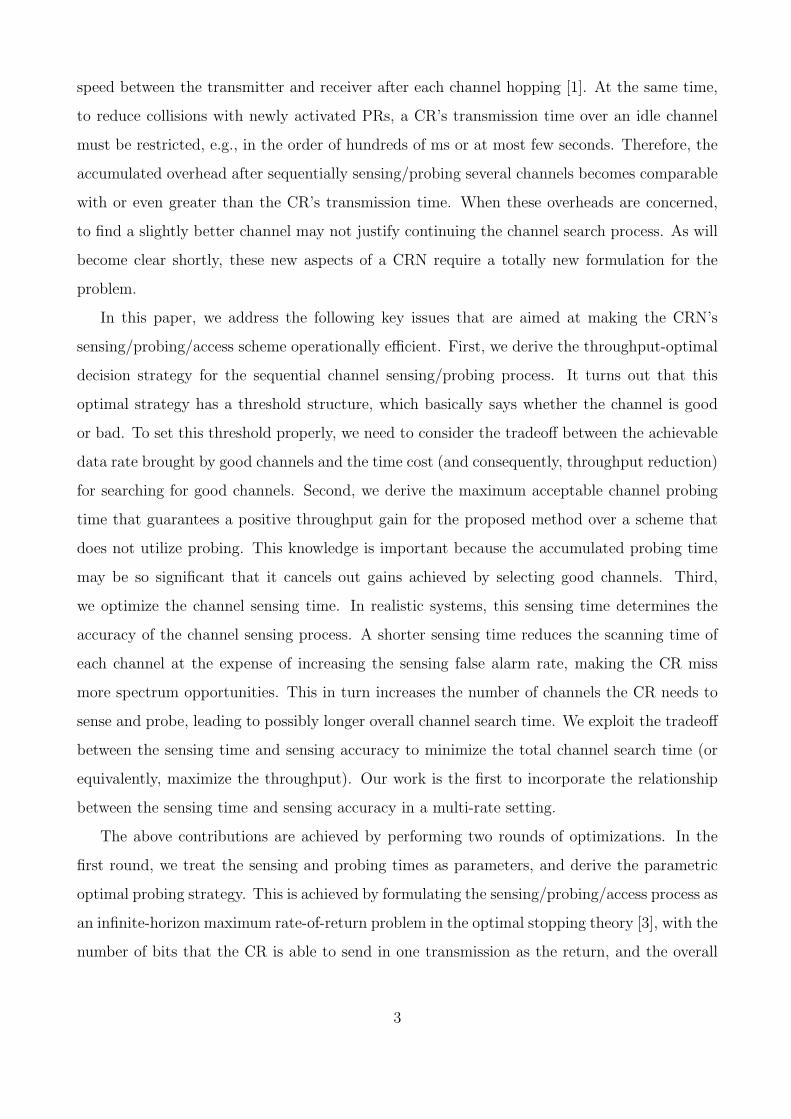
parameters γ, τmins , Pmd, and fs, we suggest an exponential curve fitting for (21), yielding

Pfa(τs) ≈ e−bτs . Mathematically, this fitting is inspired by the well-known approximation [16]

erfc(x) ≤ e−x2. Numerically, we found that this exponential fitting achieves good accuracy.

Figure 2 shows an example when γ = 0.01, τmins = 0.1 ms, Pmd = 1%, and fs = 1 MHz. The

average fitting error in this case is less than 8%.

Applying the exponential fitting of Pfa(τs) and treating τs as the variable, the domain of

the jth segment defined in (17) now becomes:

(1− e−bτs)Cjτt < τs + τp ≤ (1− e−bτs)Cj−1τt. (23)

The above partition is not in explicit form of τs because τs appears on both sides of each

inequality. To get the explicit partitions, we need to solve the following series of equations of

12

0 20 40 60 80 10010

−8

10−6

10−4

10−2

100

Sensing time (ms)

Fal

se a

larm

rat

e

actual valueexponential curve fitting

SNR=0.02, Pmd

=1%,fs=1 MHz

Figure 2: Exponential curve fitting of the false alarm rate.

τs:

τs = (1− e−bτs)Cjτt − τp, 1 ≤ j ≤ K. (24)

For each equation, if a non-negative solution exists, then it gives a partition point over τs. The

difficulty here is that such a solution does not always exist.

Theorem 4: The following four statements specify the existential condition and structure of

the solutions to (24):

1. Existential condition: An equation in (24) has solutions if and only if Cjτt− 1b− 1

bln bCjτt ≥ 0;

2. Number of solutions: Each equation in (24) can have at most two solutions. At most one

equation can have exactly one solution;

3. Sign of solutions: If an equation has two solutions, then both solutions are positive (or

negative) if 1bln bCjτt is positive (or negative). In other words, it is impossible to have one

positive solution and one negative solution for the same equation;

4. Structure of solutions: If the jth equation has two positive solutions, denoted as τ(j,high)s and

τ(j,low)s , where τ

(j,high)s ≥ τ

(j,low)s > 0, then the (j−1)th equation must have two positive solutions,

which satisfy the condition τ(j−1,high)s > τ

(j,high)s ≥ τ

(j,low)s > τ

(j−1,low)s > 0.

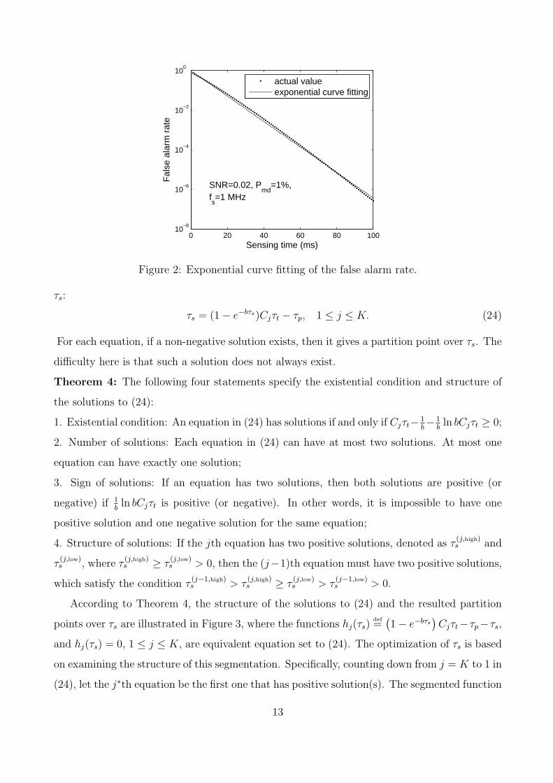
According to Theorem 4, the structure of the solutions to (24) and the resulted partition

points over τs are illustrated in Figure 3, where the functions hj(τs)def=

(1− e−bτs

)Cjτt−τp−τs,

and hj(τs) = 0, 1 ≤ j ≤ K, are equivalent equation set to (24). The optimization of τs is based

on examining the structure of this segmentation. Specifically, counting down from j = K to 1 in

(24), let the j∗th equation be the first one that has positive solution(s). The segmented function

13

sτ

)( sKh τ

)(* sjh τ

)(1 sh τ

)*,( highjsτ)*,( lowj

sτ ),1*( highjs

−τ),1*( lowj

s−τ ),1( high

sτ),1( low

sτ

)( sjh τ

)(1* sjh τ−

Figure 3: Structure of the solutions to (24) and the partition points over τs.

λ∗(τs) is described as follows: 1. The total number of segments is 2j∗ + 1. 2. The domain of

these segments are given from left to right by [0, τ(1,low)s ), [τ

(1,low)s , τ

(2,low)s ), . . ., [τ

(j∗,low)s , τ

(j∗,high)s ),

[τ(j∗,high)s , τ

(j∗−1,high)s ), . . ., [τ

(1,high)s ,∞). 3. Recalling the condition (15) required for λ∗, for the

jth left-most and the jth right-most segments, where 1 ≤ j ≤ j∗, the corresponding λ∗ must

satisfy (1 − Ploss)Rj−1 < λ∗ ≤ (1 − Ploss)Rj. In addition, the specific value of λ∗ in these two

segments is given by

λ∗ =(1− e−bτs)τtPI(1− Ploss)

∑Kk=j Rkpk

τs + τp + (1− e−bτs)τtPI

∑Kk=j pk

. (25)

Three properties regarding this segmentation can be observed: 1. Inside each segment,

the relationship between λ∗ and τs, i.e., (25), is no longer convex or monotonic. So λ∗ is

in general neither convex nor monotonic for the entire domain τs ≥ 0. 2. Interestingly, the

trend of λ∗ is concave if we treat segment as our observation unit: Starting from the left-

most segment, [0, τ(1,low)s ), any τs in the next segment gives greater λ∗ than what any τs in

the previous segment gives. This trend is valid until reaching the segment in the middle,

[τ(j∗,low)s , τ

(j∗,high)s ). Starting from this segment and until the last one, any τs in the next segment

gives smaller λ∗ than what any τs in the previous segment gives. 3. The segment in the

middle gives λ∗s that are greater than in any other segments. In other words, we can define

Tos

def= {τs : τ

(j∗,low)s ≤ τs ≤ τ

(j∗,high)s )}. To

s is a closed range that contains the optimal τ os . In

14

addition, any τs ∈ Tos achieves greater throughput than any τ ′s /∈ To

s, and its throughput is

bounded by (1 − Ploss)Rj∗ ≤ λ∗ ≤ (1 − Ploss)Rj∗+1. Therefore, for the sensing/probing/access

scheme, even though we cannot find τ os explicitly, we can still decide a good range for τs that

gives provably near-optimal performance.

Lemma 1: The closed range Tos is

Rj∗Rj∗+1

-optimal, i.e., any τs ∈ Tos can achieve at least

Rj∗Rj∗+1

fraction of the maximum throughput, where j∗ denotes the id of the first equation that has

positive solution(s) when counting down from the Kth to the first equation defined in (24).

4 Throughput Analysis for CRNs

In this section, we study the aggregate network throughput when several CRs share the same

spectrum, each being driven by its own sensing/probing/access process discussed before. An

important factor we need to consider in this scenario is collisions between CRs, i.e., more than

one pair of CR transmitter/receiver may be sensing the same channel at the same time, so none

of them can use the channel even if this channel is idle and is of a good quality.

We consider two sensing strategies for the CRs: random channel sensing and collaborative

channel sensing. In random channel sensing, each CR pair randomly selects a channel to sense

in each step. There is no information exchange between different CR pairs. For collaborative

sensing, CRs exchange their channel-hopping information in every step to avoid multiple CRs

hopping to the same channel at the same time.

A discrete-time Markov-chain model is used to analyze the throughput of the CRN. Time

is divided into slots with slot length τs + τp. So for a CR, each step of channel sensing/probing

takes exactly one slot and each transmission takes Ldef= d τt

τs+τpe slots. We assume that CRs

are synchronized, i.e., the slots of different CRs are aligned. Let the number of CR transmit-

ter/receiver pairs be M . To simplify the presentation, here we only consider the fundamental

case when each CR link can only sense, probe, and transmit over one channel at a time. The

case that a CR link can simultaneously use J > 1 channels can be treated as J indepen-

dent one-channel virtual CR links and analyzed accordingly. To evaluate the CRN’s capability

of harvesting the spectrum, we are interested in a saturated traffic scenario, i.e., there is al-

ways backlogged traffic at each CR link. The state of the Markov chain is defined as a tuple

(x1, . . . , xM), where each element xm ∈ {0, 1} stands for the activity of the mth CR link in the

current slot: xm = 0 means that CR link m is sensing and probing a channel; xm = 1 denotes

15

0 50 100 150 2000.2

0.4

0.6

0.8

1

1.2

1.4

1.6

Channel probing time (ms)

Thr

ough

put (

Mbp

s)

with probingwithout probing

τs=10 ms, τ

t=500 ms

good channel condition

poor channel condition

Figure 4: Throughput vs.probing time.

0 50 100 150 2000.2

0.3

0.4

0.5

0.6

0.7

0.8

0.9

1

Sensing time (ms)

Thr

ough

put (

Mbp

s)

poor channel conditiongood channel condition

TSo

TSo

Figure 5: Throughput vs. sens-ing time.

5 10 15 200

1

2

3

4

5

6

7

Number of channels

CR

N th

roug

hput

(M

bps)

random sensing w/ probingrandom sensing w/o probingcollaborative sensing w/ probingcollaborative sensing w/o probing

Figure 6: CRN throughput vs.number of channels.

an ongoing transmission by that link. The CR links’ activities in the current slot are mutually

independent, but are related to all CR links’ activities in the previous slot, (x′1, . . . , x′M), i.e.,

the transition probability of the chain has the following property

Pr(x1, . . . , xM |x′1, . . . , x′M) =M∏

m=1

Pr(xm|x′1, . . . , x′M) (26)

This property is reasonable, because a CR’s activity in the current slot should depend only on

its observation of other CRs’ activities in the previous slot.

Without loss of generality, we consider the transition probability of CR link 1. We first

consider the random sensing strategy. The calculation includes the following four cases:

Case 1: Pr(0|0, x′2, . . . , x′M)

In this case, the transition probability contains four components

Pr(0|0, x′2, . . . , x′M) = Pcr occupied + Pcr collision + Ppr occupied

+Ppoor channel (27)

where Pcr occupied denotes the probability that the channel sensed/probed by CR link 1 in the

previous slot was being used (transmitted over) by other CR links; Pcr collision denotes that even

though the situation described in Pcr occupied did not happen, the channel sensed/probed by CR

link 1 in the previous slot was also sensed/probed by at least another CR links in the same

slot; Ppr occupied denotes that even though the two situations in Pcr occupied and Pcr collision did

not happen, the channel sensed/probed by CR link 1 in the previous slot was being occupied

by PRs; Ppoor channel denotes that even though the three situations in Pcr occupied, Pcr collision,

and Ppr occupied did not happen, the channel sensed/probed by CR link 1 in the previous slot

was having a bad channel condition, i.e., its MADR is below the channel quality threshold.

16

To calculate these four probabilities, we note that a collision of multiple CRs sensing the

same channel can be detected during the probing operation. After detecting a collision, the

CRs will sense/probe other channels in the next slot. Therefore a CR’s transmission over some

channel indicates this channel is collision-free between CRs. We define the following notations:

M(m)1

def=

∑Mi=1;i6=m x′i and M

(m)0

def= (M − 1) −M

(m)1 . M

(m)1 denotes the number of transmitting

CR links in the previous slot, not counting the mth link; M(m)0 is the number of sensing/probing

channels in the previous slot, not counting the mth link. Then we can calculate

Pcr occupied =M

(1)1

C(28)

Pcr collision =

(1− M

(1)1

C

)1−

(C − 1

C

)M(1)0

(29)

Ppr occupied =

(1− M

(1)1

C

) (C − 1

C

)M(1)0

QB (30)

Ppoor channel =

(1− M

(1)1

C

)(C − 1

C

)M(1)0

QI

k∗−1∑

k=0

pk (31)

Case 2: Pr{1|0, x′2, . . . , x′M}This transition probability is simply given by

Pr{1|0, x′2, . . . , x′M} = 1− Pr{0|0, x′2, . . . , x′M}

=

(1− M

(1)1

C

) (C − 1

C

)M(1)0

QI

K∑

k=k∗pk (32)

Case 3: Pr{0|1, x′2, . . . , x′M}This case means that CR link 1 finished its transmission in the previous slot, so it starts looking

for a new channel in the current slot. The transition probability is given by

Pr{0|1, x′2, . . . , x′M} = 1/L (33)

Case 4: Pr{1|1, x′2, . . . , x′M}This is simply calculated as

Pr{1|1, x′2, . . . , x′M} = 1− Pr{0|1, x′2, . . . , x′M} = (L− 1)/L. (34)

17

Having obtained the transition probability matrix, the Markov chain’s stationary distribution

for the random vector (x1, . . . , xM) can be calculated using standard state-transition balance

equations. Among all the states, those with∑M

m=1 xi > C are infeasible, and therefore their

stationary distribution probability is 0. The CRN’s throughput is then calculated as

Rtot =1∑

x1=0

. . .

1∑xM=0

Pr{x1, . . . , xM}M∑

m=1

xmR̄ (35)

where R̄def=

(1−Ploss)∑K

k=k∗ Rkpk∑Kk=k∗ pk

is the average throughput a CR link can achieve when it is

transmitting.

In the above calculation, we have assumed a fully-distributed random channel sensing strat-

egy. When a collaborative sensing strategy is used, then the above calculation should be

modified as follows: the term,(

C−1C

)M(1)0 , should be replaced by

(C−1

C

)max(0,M(1)0 +1−C)

in (28)

through (32). This is because under collaborative sensing, if the number of links that are sens-

ing channels is not greater than the number of channels, then there is no collision. Otherwise

the collision is only due to those links that exceed the number of channels.

5 Numerical Examples

We first consider the optimal throughput of a single CR link as a function of various operational

parameters. We assume a discrete-rate CR system that supports four rates: 1, 2, 3, and

4 Mbps. We consider the rate distribution, (p0, p1, p2, p3, p4), under two channel conditions:

a good channel condition with rate distribution of (0.1, 0.1, 0.2, 0.2, 0.4) and a poor channel

condition with rate distribution (0.4, 0.2, 0.2, 0.1, 0.1). We assume that the average idle and

busy time of each channel is α = β = 500 ms.

In Figure 4, we plot the throughput of the sensing/probing/access scheme as a function

of the channel probing time. The channel sensing and transmission times are fixed at 10

ms and 500 ms, respectively. We assume that Pfa = 0.1. The throughput of the CR link

when probing is not used is also plotted for comparison. It is clear that as long as τp is kept

sufficiently small, i.e., τp < 45 ms under good channel conditions or τp < 100 ms under poor

channel conditions, the use of probing leads to throughput gains over the scheme that does not

use probing. Recalling that the reported per-channel probing time in current 802.11 WLAN

systems ranges from 10 to 133 ms [1], the above probing time requirement is non-trivial, because

there is still a reasonable chance under the current technology that the use of probing could

18

actually undermine the throughput. In addition, the effect of probing is more significantly

observed under poor channel conditions, e.g., the throughput gain reaches about 120% when

τp = 10 ms. At the same time, the maximum acceptable channel probing time becomes 100

ms. These results favor the use of probing when the channel condition is bad, which is in line

with our intuition.

Figure 5 depicts the throughput as a function of the channel sensing time. Here we use the

exponential curve fitting for the Pfa—τs relationship with parameter b = 14.8349. The concave

trend of the throughput as function of τs can be clearly observed in this figure. More impor-

tantly, even though we cannot analytically derive the globally optimal τ os that maximizes the

throughput, our analysis in section 3 shows that they must be located in the ranges denoted by

the dotted boxes, i.e., τ os ∈ [15.1, 43.9] ms under good channel conditions, and τ o

s ∈ [6.8, 140.5]

ms under poor channel conditions. The sensing time in practical operations should be controlled

within these ranges to achieve bounded near-optimal throughput.

Next, we use the optimal threshold derived for individual links to drive the operation of

CRN. In Figures 6, we fix the number of CR links M = 8 and plot the CRN throughput as

a function of number of channels, C. The rate distribution for each CR link is given by (0.2,

0.2, 0.2, 0.2, 0.2). We set τs = τt = 10 ms, and τt = 500 ms. It is clear that the collaborative

sensing strategy achieves greater throughput than the random sensing strategy, largely due to

the smaller collision probability under collaborative sensing. In addition, it can be observed

that under both strategies, the CRN throughput in general increases with C. However, the

speed of increase is fast when C is small, and becomes slow when C is large. This trend is

due to the smaller collision probability and the more likelihood of finding an idle channel when

C is large. A third observation is that in the case of collaborative sensing, the slope of the

throughput curve is less steep than in the random sensing case when C is large. This is because

the collision probability under collaborative sensing has become 0 when C is large, and therefore

the throughput increase is only due to the increased probability of finding a good idle channel.

6 Related Work

In existing literature on DSS schemes, sensing is the only operation performed by CRs to select

channels. The problem of finding a good channel is reduced to finding an idle one. Based on the

assumptions about the sensing overhead and sensing accuracy, these works can be classified into

19

three types. The first type assumes negligible sensing time and an accurate sensing outcome

(i.e., zero false alarm and miss detection rates). Under this highly idealized sensing model, these

work usually focus on other aspects of DSS. For example, the work in [12], [7], and [17] study

the collision issues between a transmitting CR and a returning PR by optimizing the CR’s

transmission time, the distribution of the CR’s transmission time, and the CR’s probability of

transmission, respectively. The second body of works assumes a non-negligible sensing time

and an accurate sensing outcome. Among them, the work in [10] minimizes the time cost of

finding an idle channel by optimizing the sensing frequency and the sensing sequence of different

channels. A similar problem is investigated in [19] under partial channel observability, whereby

a CR can only sense a small subset of channels in order to find one available. The work in

[9] considers the scenario that a CR can transmit over multiple channels simultaneously, but

these channels have to be found in a sequential manner (one after another). The problem is to

decide an optimal number of idle channels the CR should use such that the average throughput,

which accounts for the aggregate rate provided by the combined channels and the time cost

on finding these channels, is maximized. The third body of works assumes a realistic sensing

model, whereby the sensing accuracy becomes a function of the sensing time. These works aim

at exploiting the tradeoff between the sensing time and the sensing accuracy for the purpose of

minimizing the time latency of finding an idle channel [4] or maximizing the throughput of a CR

link [11][6]. Compared with these previous work, the use of probing significantly complicates

the channel selection problem, because only finding idle channels is no longer sufficient; we need

to find good idle channels. Furthermore, our work is the first to incorporate the relationship

between the sensing time and sensing accuracy in a multi-rate setting.

Channel probing has been comprehensively studied for general wireless systems under the

assumption that the probing overhead is negligible [14]. However, joint optimization of the

reward obtained from channel selection and the cost incurred by channel probing only recently

started to receive attention. There are a few related work, but all of them are for wireless

systems with dedicated channels, e.g, [15, 2, 21, 20, 8, 5, 22]. The difference between our

problem and the previous work includes the following: First, the problem of combined channel

sensing and probing has not been considered in all existing works. The inclusion of sensing in

the channel selection problem is non-trivial, because the sensing time can affect the throughput

by non-linearly changing the channel sensing accuracy. Second, previous work on channel

probing involves only a relatively small channel pool, e.g., a pool of 3 channels for 802.11

20

and 8 channels for 802.11a. For CRNs, this pool can be much larger. As a result, those

algorithms designed for small channel pools, e.g., the finite-horizon stopping method in [15]

and the tree-based searching algorithm in [5, 8], become practically infeasible in CRNs because

of the prohibitive computational complexity when the number of channels is large. In our work,

an infinite-horizon formulation is employed, which is particularly suitable for modeling large

channel pools. Third, the ultimate concern of all previous work is the optimal probing strategy

that maximizes the throughput. In this work, we are not only interested in the optimal probing

strategy, but also in the particular structure of this strategy, with the objective of performing

a second-round optimization over operational parameters such as the sensing time and the

probing time. Fourth, we also study the aggregate throughput for a network of CRs, in which

collisions between CRs during sensing and probing is possible. Nearly all related work has

ignored this fact and only considered the single-link case in their analysis.

7 Conclusions

Our study has indicated that a carefully-designed joint channel sensing and probing scheme

for CRNs can achieve significant throughput gains over the conventional mechanism that uses

sensing alone. Our findings include: (1) The throughput-optimal probing strategy has a thresh-

old structure, which basically judges whether a channel is good or bad when being probed, (2)

To achieve throughput gain over the conventional sensing approach, the probing time has to

be smaller than some explicit upper bound; otherwise using sensing alone can achieve better

throughput, (3) When probing is used, the throughput in general is no longer a concave function

of the sensing time, largely due to the more complicated multi-rate structure induced by the

addition of probing. However, this function has a segmented structure. If we treat segments

as our observation units, the trend of this function is concave. We exploited this property

to derive a closed range for the sensing time that provides provably near-optimal throughput

performance.

A. Proof of Theorem 1

Proof: 1. Existence. We need to prove that for any finite λ, an optimal stopping rule exists for

the transformed problem (12). It follows from Theorem 1 in Chapter 3 of [3] that the optimal

stoping rule exists if the following two conditions are satisfied:

1. E{supn wn} < ∞.

21

2. limn→∞ supn wn = −∞, a.s.

By examining (12), condition 2 is clearly satisfied. Condition 1 can be proved by applying

Theorem 1 in Chapter 4 of [3]. Specifically, it is easy to see that the random variable

X ′n

def= Xnτt(1− Ploss)− λτt (36)

is only related to the random variable Xn. Because Xn’s are i.i.d. for all n = 1, . . ., X ′n’s must

also be i.i.d.. In addition, because Xn takes a finite number of values and λ is finite, X ′n must

also be finite. Therefore, it holds that E{max(X ′n, 0)} < ∞ and E{(max(X ′

n, 0))2} < ∞. So

according to Theorem 1 in Chapter 4 of [3], it holds that E{supn wn} = E{supn X ′n − nλ(τs +

τp)} < ∞. So condition 1 is also satisfied.

2. The optimal solution. wn can be written as wn = X ′n − nλ(τs + τp), where X ′

n is defined

in (36). So X ′n can be considered as the reward for observing w1, . . . , wn, and λ(τs + τp) can

be deemed as the cost for each observation. Applying the principle of optimality in Chapter 2

of [3], the optimal stopping rule of the transformed problem (12) is given by

N∗ = min{n ≥ 1 : X ′n ≥ V ∗} (37)

where V ∗ denotes the expected return from an optimal stopping rule; it satisfies the following

optimality equation

V ∗ = E{max{X ′n, V

∗}} − λ(τs + τp). (38)

Equivalently, the above equation can be written as

E{max(X ′n − V ∗, 0)} = λ(τs + τp). (39)

Recalling the connection between the original problem and its transformed version, the value

of λ that gives V ∗ = 0 is simply the solution of (11). With V ∗ = 0, we have the following

equation:

E{max(Xnτt(1− Ploss)− λ∗τt, 0)} = λ∗(τs + τp) (40)

According to Theorem 1 in Chapter 6 of [3], the solution of the above equation, λ∗, is the

maximum objective function value for problem (11). At the same time, substituting V ∗ = 0

into (37), we derive the optimal stopping rule to problem (11):

N∗ = min{n ≥ 1 : Xn ≥ λ∗

1− Ploss

} (41)

22

This concludes the proof of Theorem 1.

B. Proof of Theorem 2

Proof: The main idea is to show that the LHS of (40) is a mono-decreasing function in λ∗ while

the RHS is mono-increasing of λ∗. They must intersect at one and only one point. Particularly,

we define g(λ) = E{max(Xnτt(1−Ploss)−λτt, 0)}. For the general case of a continuous random

variable Xn with pdf q(x), g(λ) can be extended as

g(λ) =

∫ ∞

λ1−Ploss

xτt(1− Ploss)q(x)dx−∫ ∞

λ1−Ploss

λτtq(x)dx. (42)

The first-order derivative of g is given by

dg(λ)

dλ= −λτtq

(λ

1− Ploss

)

−[τt

∫ ∞

λ1−Ploss

q(x)dx− λτtq

(λ

1− Ploss

)]

= −2λτtq

(λ

1− Ploss

)− τt

∫ ∞

λ1−Ploss

q(x)dx. (43)

Clearly, both terms in (43) are strictly negative, and therefore g(λ) is a strictly mono-decreasing

function. In addition, g(0) = τt(1 − Ploss)E[Xn] < ∞ and g(∞) = 0. It is clear that the RHS

of (40) is a strictly mono-increasing function of λ with function values of 0 and ∞ when λ = 0

and λ = ∞, respectively. For the case of discrete random variable Xn, it is easy to see that the

above monotonic property does not change. Therefore, λ∗ must have a unique solution.

C. Proof of Theorem 3

Proof: First, by evaluating λ∗j(η), it is clear that inside each segment, λ∗ is continuous and

strictly mono-decreasing. Next, it can be easily verified that Φj = φj−1 and limη→Φjλ∗j(η) =

λ∗j−1(φj−1) for j = 2, . . . , K. Therefore, λ∗ is continuous and strictly mono-decreasing over the

entire domain of η.

D. Proof of Theorem 4

Proof: 1. We first prove the existential condition. Define

hj(τs) =(1− e−bτs

)Cjτt − τp − τs, 1 ≤ j ≤ K. (44)

This function is concave since its second-order derivative is:

d2hj

dτ 2s

= −b2Cjτte−bτs < 0. (45)

23

Because of this concavity, it is clear that hj(τs) = 0 has solutions if and only if the function’s

maximum value is not smaller than 0. The maximum value is calculated as follows:

dhj

dτs

= e−bτsbCjτt − 1 = 0. (46)

From (46) we can get τ os = 1

bln bCjτt. Accordingly, the maximum value of hj(τs) is given by

hmaxj

def= hj(τ

os ) = Cjτt − 1

b− 1

bln bCjτt (47)

Then statement 1 follows.

2. The first half of Statement 2 is clear due to the concavity of hj(τs). We prove the second

half after Statement 4.

3. The proof is based on contradiction. We first consider the case when τ os = 1

bln bCjτt > 0.

From the concavity of hj, it is clear that at least one solution must be positive. Now suppose

the second solution is negative. Then hj(0) ≥ 0 must hold. However, from (44), when τs = 0,

hj(0) = −τp < 0. Similar contradiction can be established when τ os = 1

bln bCjτt < 0. So

Statement 3 holds.

4. From the definition of Cj in (20), it is clear that Cj < Cj−1. Now consider the solution

τ(j,high)s of the jth equation. From (24), we have

τ (j,high)s = (1− ebτ

(j,high)s )Cjτt − τp < (1− ebτ

(j,high)s )Cj−1τt − τp. (48)

As τs → ∞, it holds that limτs→∞(1 − e−bτs)Cj−1τt − τp = Cj−1τt − τp < ∞. So the function

(1 − e−bτs)Cj−1τt − τp must intersect with the function τs between τ(j,high)s and ∞ (the two

boundaries not included). Applying a similar logic to τ(j,low)s , it is clear that the function (1−

e−bτs)Cj−1τt − τp also intersects with the function τs between 0 and τ(j,low)s (the two boundaries

not included). Note that the two domains (τ(j,up)s , ∞) and (0, τ

(j,low)s ) do not overlap with each

other. Accounting for Statements 2 and 3, it can be concluded that there are only two solutions

to the (j − 1)th equation, each of which are positive. One solution is located in (τ(j,high)s , ∞)

and the other located in (0, τ(j,low)s ). So Statement 4 follows.

Based on Statement 4, the second half of Statement 2 is straightforward: Counting down

from j = K to 1, the first equation, say the j∗th one, that has solutions is the only one that

can have exactly one solution. For all j < j∗, each equation must have two solutions.

24

References

[1] W. Arbaugh. Improving the latency of the probe phase during 802.11 handoff, [online]

available: http://www.umiacs.umd.edu/partnerships/ltsdocs/arbaug-talk2.pdf.

[2] N. B. Chang and M. Liu. Optimal channel probing and transmission scheduling for op-

portunistic spectrum access. In Proceedings of the ACM MobiCom Conference, 2007.

[3] T. Ferguson. Optimal stopping and applications. Available online at

http://www.math.ucla.edu/ tom/stopping/content.html.

[4] A. Ghasemi and E. S. Sousa. Optimization of spectrum sensing for opportunistic spectrum

access in cognitive radio networks. In Proceedings of the IEEE Consumer Communication

Networking Conference (CCNC), pages 1022–1026, Jan. 2007.

[5] S. Guha, K. Munagala, and S. Sarkar. Optimizing transmission rate in wireless channels

using adaptive probes. In ACM Sigmetrics/Performance Conference, 2006. Poster paper.

[6] A. T. Hoang and Y. C. Liang. Adaptive scheduling of spectrum sensing periods in cognitive

radio netwroks. In Proceedings of the IEEE GLOBECOM Conference, pages 3128–3132,

2007.

[7] S. Huang, X. Liu, and Z. Ding. Opportunistic spectrum access in cognitive radio networks.

In Proceedings of the IEEE INFOCOM Conference, pages 1427–1435, Apr. 2008.

[8] Z. Ji, Y. Yang, J. Zhou, M. Takai, and R. Bagrodia. Exploiting medium access diversity

in rate adaptive wireless LANs. In Proceedings of the ACM MobiCom Conference, pages

345–359, Sept. 2004.

[9] J. Jia, Q. Zhang, and X. Shen. HC-MAC: A hardware-constrained cognitive MAC for

efficient spectrum management. IEEE Journal on Selected Areas in Communications,

26(1):106–117, Jan. 2008.

[10] H. Kim and K. G. Shin. Efficient discovery of spectrum opportunities with MAC-layer

sensing in cognitive radio netwroks. IEEE Transactions on Mobile Computing, 7(5):533–

545, May 2008.

25

[11] Y. C. Liang, Y. Zeng, E. C. Y. Peh, and A. T. Hoang. Sensing-throughput tradeoff for

cognitive radio networks. IEEE Transactions on Wireless Communications, 7(4):1326–

1337, Apr. 2008.

[12] X. Liu and S. N. Shankar. Sensing-based opportunistic channel access. ACM Journal of

Mobile Networks and Applications, 11(4):577–591, Aug. 2006.

[13] J. Mitola. Cognitive radio: an integrated agent architecture for software defined radio.

PhD Dissertation, RTH, Sweden, May 2000.

[14] T. S. Rappaport. Wireless Communications: Principles & Practice. Prentice Hall, 2002.

[15] A. Sabharwal, A. Khoshnevis, and E. Knightly. Opportunistic spectral usage: bounds and

a multi-band CSMA/CA protocol. IEEE/ACM Transactions on Networking, 15(3):533–

545, June 2007.

[16] J. M. Wozencraft and I. M. Jacobs. Principles of Communication Engineering. London:

John Wiley & Sons, Inc, 1965.

[17] Q. Zhao, S. Geirhofer, L. Tong, and B. M. Sadler. Optimal dynamic spectrum access via

periodic channel sensing. In Proceedings of the IEEE WCNC Conference, 2007.

[18] Q. Zhao and B. M. Sadler. A survey of dynamic spectrum access: signal processing,

networking, and regulatory policy. IEEE Signal Processing Magazine, 24(3):79–89, 2007.

[19] Q. Zhao, L. Tong, A. Swami, and Y. Chen. Decentralized cognitive MAC for opportunistic

spectrum access in ad hoc networks: a POMDP framework. IEEE Journal on Selected

Areas in Communications, 25(3):589–600, Apr. 2007.

[20] D. Zheng, M. Cao, J. Zhang, and P. R. Kumar. Channel aware distributed scheduling for

exploiting multi-receiver diversity and multiuser diversity in ad-hoc networks: a unified

phy/mac approach. In Proceedings of the IEEE INFOCOM Conference, pages 1454–1462,

2008.

[21] D. Zheng, W. Ge, and J. Zhang. Distributed opportunistic scheduling for ad-hoc commu-

nications: an optimal stopping approach. In Proceedings of the ACM MobiHoc Conference,

2007.

26

[22] D. Zheng and J. Zhang. Joint optimal channel probing and transmission in collocated

wireless networks. In Proceedings of the IEEE INFOCOM Conference, pages 2266–2270,

May 2007.

27