TECHNICAL PUBLICATION EMA # 399 FLOW MONITORING IN STORMWATER TREATMENT AREA NO. 6 By Muluneh Imru Senior Engineer December 2001 Hydrology and Hydraulics Division Environmental Monitoring & Assessment Department South Florida Water Management District West Palm Beach, Florida

Welcome message from author
This document is posted to help you gain knowledge. Please leave a comment to let me know what you think about it! Share it to your friends and learn new things together.
Transcript

TECHNICAL PUBLICATION EMA # 399
FLOW MONITORING IN STORMWATER
TREATMENT AREA NO. 6
By Muluneh Imru
Senior Engineer
December 2001
Hydrology and Hydraulics Division Environmental Monitoring & Assessment Department
South Florida Water Management District West Palm Beach, Florida


i
EXECUTIVE SUMMARY This report describes the criteria, equations and procedures used to quantify flow through Stormwater Treatment Area No. 6 (STA-6). To evaluate the performance of STA-6 in terms of phosphorus reduction, it is essential that flows into and out of this constructed wetland be estimated using rigorous methods. This poses a challenge due to the configuration of the hydraulic structures and the complexity of water movement through the system. Flow control structures at STA-6 include trapezoidal weirs (G601, G602 and G603) for inflow, and culverts with weir-box inlets (G354 and G393) for outflow. STA-6 receives agricultural drainage delivered through the pumps at G600. In STA-6, like in several other District sites, two or more structure types are built next to each other. At such sites, there is no separate stage monitoring for each structure type. This is especially true where a typical structure is a culvert with a weir-box inlet (G354 and G393). While culvert flow conditions prevail over the downstream portion of such a combination structure, weir flow characteristics may dominate at the inlet. The weir box at the inlet of a typical culvert in STA-6 is needed to retain water in the treatment cell and keep it wet as much as possible. Procedures have been developed to monitor all inflows and outflows at STA-6 Section 1. The criteria and steps to be followed for computing flows into STA-6 cells through the inflow weirs have been established. A method has been presented that will enable the computation of flow through the weir box and gated-culvert combination structures at G354 and G393 (weir-culvert) in order to monitor outflows from each cell. Data derived from these methods are validated by a good correlation between inflows at G600 and outflows through G354 and G393. The flows through G601, G602 and G603 are slightly different from G600 inflows, as well as the outflows through G354 and G393. There is room for improvement of the weir inflow estimates. It is also possible to gain some improvement on the overall accuracy of flow computation at STA-6 structures through streamgauging and calibration. The criteria, equations and procedures developed for STA-6 can, with applicable adaptations, be used for flow monitoring at similar stations in other stormwater treatment areas when they come on line. The adaptations will primarily involve determining site- specific coefficients for similar structure types on the basis of streamgauging data.

ii
CONTENTS
1.0 INTRODUCTION………………………………………………………… ........................ 1
2.0 OBJECTIVES……………………………………………………………………... ............ 3
3.0 WEIR FLOW EQUATIONS……………………………………………………... .............. 3
3.1 DISCHARGE THROUGH WEIRS OF RECTANGULAR FLOW SECTION…………………………………………………………………………. ............ 4
3.1.1 FREE WEIR FLOW……………………………………………………………. .............. 4
3.1.2 SUBMERGED WEIR FLOW………………………………………………….. .............. 6
3.2 DISCHARGE THROUGH WEIRS OF TRAPEZOIDAL SECTION………… ................. 7
3.2.1 FREE WEIR FLOW……………………………………………………………. ............... 8
3.2.2 SUBMERGED FLOW…………………………………………………………................ 9
3.2.3 OVERTOPPED WEIR FLOW…………………………………………………............... 9
3.2.4 ZERO FLOW…………………………………………………………………................ 10
3.2.5 REVERSE FLOW……………………………………………………………... ............. 10
4.0 CULVERT FLOW EQUATIONS………………………………………………............... 10
4.1 CRITICAL FLOW IN CULVERTS……………………………………………................ 11
5.0 FLOW EQUATIONS FOR GATED CULVERTS WITH WEIRS…………... ................. 14
5.1 FULL CULVERT FLOW………………………………………………………................ 15
5.2 CULVERT PARTIALLY SUBMERGED……………………………………… .............. 15
5.3 SUBCRITICAL FREE SURFACE FLOW THROUGHOUT THE CULVERT.. .............. 16
6.0 COMPUTATION OF INFLOW THROUGH WEIRS G601 AND G602……. ................. 17

iii
7.0 COMPUTATION OF INFLOW THROUGH WEIR G603…………………... ................. 18
8.0 COMPUTATION OF OUTFLOW THROUGH G354 AND G393………….................... 19
9.0 FLOW ESTIMATION PARAMETERS……………………………………….. ............... 22
10.0 EVALUATION OF FLOW ESTIMATES…………………………………….. ............... 25
11.0 CONCLUSIONS AND RECOMMENDATIONS……………………………... .............. 29
REFERENCES…………………………………………………………………………. ............ 30
APPENDIX I STA-6 INFLOW, INTERIOR AND OUTFLOW STAGES
FOR OCTOBER 2000……………………………………………………………............ 31
APPENDIX II STA 6 INFLOWS AND OUTFLOWS THROUGH CELL 5
FOR OCTOBER 2000….…………………………………………………………........... 51

iv
Figures Figure 1. Free Weir Flow Figure 2. Submerged Weir Flow Figure 3. Trapezoidal Flow Section Weir Figure 4. General Culvert Flow Section Figure 5. Trapezoidal/Rectangular Culvert Section Figure 6. Circular Culvert Section Figure 7. Culvert Flow Profiles Figure 8. STA-6 Instantaneous Flow of October 2000 Figure 9. STA-6 Cumulative Flow of October 2000 Figure 10. Inflow and Outflow Stages of Cell 3 October 2000 Tables Table 1. Structure information for STA-6 stations Table 2. Discharge coefficients for STA-6 stations Table 3. STA-6 Flow Monitoring Sites and Stage Stations Notation The following notations are used to characterize flow through weirs and culverts: A = flow cross section (maximum Ao) Ag = entrance cross section (gate opening) area Ao = culvert cross section area = πD2 / 4 B = culvert bottom width or weir length (bottom width of trapezoidal section) Bm = average width of trapezoidal weir section under water Be = effective weir length cd = culvert discharge coefficient cw = weir flow coefficient CW = (approach) channel width D = diameter of circular culvert or depth of box culvert Dm = mean depth (area/water surface width) e = width of bank or side of trapezoidal section under water h = tailwater depth above weir crest or above culvert invert or flow depth at
any location h1 = stage above datum upstream of inlet weir box h2 = stage above datum at upstream face of culvert inside the weir box h3 = water depth above the downstream invert elevation at the location of the
invert. h4 = tailwater depth above the downstream invert elevation. hc = critical flow depth hf = head loss due to friction hw = elevation difference between weir crest and downstream invert H = headwater depth above weir crest or above culvert invert HWE = head water elevation

v
INEL = inlet invert elevation ke = minor (entrance) loss coefficient (default Ke = 0.5) L = length of culvert barrel m = side slope(horizontal:vertical) of trapezoidal flow section n = Manning's roughness coefficient ND = vertical depth of inclined surface of trapezoidal weir (notch depth) N = number of contractions in weir flow OUTEL = outlet invert elevation w = weir depth Lw = weir width in flow direction R = hydraulic radius of culvert sf = energy gradient θ = angle at the center of the culvert subtended by the water surface/gate edge T = top width of trapezoidal section TWE = tailwater elevation v = flow velocity WCE = box weir crest elevation z = elevation difference between upstream and downstream inverts
vi
ACKNOWLEDGEMENTS I would like to acknowledge several people in the South Florida Water Management District who contributed in preparing and finalizing this report. My gratitude goes to Davies Mtundu and Robb Startzman for their support and encouragement. I would also like to express my gratitude to Carol Goff for coordinating the elaborate review process. I would like to express my appreciation to the following District staff, who reviewed the draft document and provided valuable suggestions that were helpful in revising the document: Davies Mtundu, Emile Damisse, Wossenu Abtew, Garth Redfield, Matahel Ansar, Juan Gonzalez-Castro, Scott Huebner, Martha Nungesser, Kathy Pietro, Jana Newman, Gary Goforth and Tracey Piconne. My gratitude also goes to Carrie Trutwin for her assistance with the final editorial review.

1
1.0 INTRODUCTION The Everglades Forever Act (EFA) mandated the South Florida Water Management District (District) to implement the Everglades Construction Project (ECP) as an important step for restoring and protecting the Everglades ecosystem. Stormwater Treatment Area No. 6 (STA-6) is a component of the ECP. It was constructed in 1997 and has been in operation since December 1997. STA-6 is a constructed wetland designed to reduce total phosphorus in the drainage water coming primarily from the Everglades Agricultural Area (EAA). Comprised of two parts (Northern Cell 5 and Southern Cell3), the wetland provides an effective treatment area of about 870 acres for drainage from approximately 10,400 acres of agricultural land. The inflow into STA-6 comes through G600, a pump station owned and operated by United States Sugar Corporation (USSC). Three trapezoidal weirs (G601, G602 and G603) control inflow into STA-6. Six culverts with weir-box inlets (G354A-C and G393A-C) control outflow from Cell 5 and Cell 3. Bypass flow control is provided at G604. All flows from G354, G393 and G604 are discharged out of STA-6 via the terminal structure (culvert) G607. Flow monitoring is conducted at more than 400 water control structures in the District. The major types of flow monitoring stations include spillways, weirs, culverts, pumping stations and open channel reaches. At many of the flow monitoring sites in the District, flow is controlled by one type of structure. In such a case, the flow monitoring equations used are those appropriate for the particular structure. However, at some sites two or more structure types are joined in series affecting flow through the station. At such sites, there is not enough space between the structures to assess the independent effects of each structure on the flow. There is no separate stage monitoring for each structure type. This is especially true at those sites whose typical structure is a weir-culvert combination, i.e., where a weir box discharges directly into a culvert. While culvert flow conditions prevail over the downstream portion of such a combination structure, the flow characteristics of the inlet may be those of a weir. At the outlets of STA-6, as in other STAs, there are gated culverts with weir-box inlets. The weir box at the inlet of a typical culvert in STA-6 helps to retain some water in the treatment cells to keep the treatment cells moist at all times (EES 1997). The inflow into the culvert is affected by the presence of the weir box at the inlet. The effects of various structure shapes and types on water flow have been investigated in the past and appropriate equations have been developed to estimate velocity, discharge and related parameters. Standard methods of computing flow through water control structures are presented in other District publications (Otero 1995). Most textbooks in hydraulics provide equations, criteria and procedures for estimating flow through a simple structure, that is, a structure consisting of only one hydraulic element, e.g. a weir. The available equations cannot, however, be directly applied when a site contains a series of joined hydraulic structures, e.g. a weir joined to a culvert (weir-box culvert). In such a structure, it is difficult to isolate the effect of each structure type on flow.

2
Figure 1. Project Location and Site Layout
A culvert with a weir type inlet poses a challenge to direct discharge estimation using existing flow computation procedures. In computing flow through a culvert with a weir inlet, several key issues need to be addressed: • identification of the control (the weir, the culvert inlet or the culvert outlet); • effects of transition from weir-controlled to culvert-controlled flow or vice-versa; • occurrence of critical flow; and • the influence of the tailwater stage on the flow. This report describes the criteria, equations and procedures used for flow monitoring in STA-6. The following section states the objectives of this report. Sections 3 through 8 present the equations and procedures used to estimate flow at STA-6 weirs and culverts. Flow estimation parameters and qualitative evaluation of flow estimates are given in Section 9 and Section 10, respectively. The last section provides conclusions and recommendations. 2.0 OBJECTIVES The overall objective of this study was to provide validated means for estimating inflows and outflows for STA-6. This work will be useful for STA-6 performance optimization research and permit compliance
3
monitoring. We currently monitor inflow into STA-6 at G600, the pumping station owned and operated by US Sugar Corporation (USSC). Water delivery into Cell 5 takes place through two inflow weirs, G601 and G602. Inflow into Cell 3 is through weir G603. Weirs G601, G602 and G603 have trapezoidal sections and, therefore, procedures are needed to compute flows into the treatment cells through the trapezoidal weirs. Outflow from STA-6 was monitored at G606, the UVM (ultrasonic velocity meter) site in the discharge canal for permit compliance until March 2001. Because of possible influences from seepage and drawdown in the supply canal, flow through the G606 UVM was, at times, different from surface outflows from the treatment cells. In order to determine STA-6 outflows, it was necessary to calculate flows at G393 and G354. The structures at G393 and G354 are weir-culvert combinations requiring a flow computation procedure different from those employed for simple structures. The purpose of this report is to document the results of planning and implementation of flow monitoring for STA-6, including: • algorithms to compute flows into the treatment cells through the trapezoidal inflow
weirs G601, G602 and G603; • algorithms to compute discharge through G393 and G354, i.e., the outlets from
Treatment Cell 3 and Treatment Cell 5, respectively; • a methodology to determine control of flow through culverts with weir-box inlets;
and • an assessment of the results of flow monitoring in STA-6. All equations are in the foot-pound-second system of units; i.e. all lengths are in feet (ft.), all weights are in pounds (lb.), and all time dimensions are in seconds (s). 3.0 WEIR FLOW EQUATIONS Discharge over a weir depends on the relative elevations of headwater, tailwater and weir crest. Depending on these relative elevations, weir flow is categorized as either free weir flow or submerged weir flow. The inflows considered in this study are uncontrolled, because there are no gates over the weirs. Since STA-6 inflow structures (G601, G602, G603) have no gates, the discussion in this study focuses on uncontrolled submerged and uncontrolled free (weir) flows. STA-6 inflow structures are broad-crested trapezoidal weirs. Many hydraulics text books provide equations for estimating discharge through broad-crested weirs. The main difference shown between sharp-crested and broad-crested weirs is that the coefficient for broad-crested weirs is a function of upstream water depth and weir depth (Chow, 1959). Other than for the coeffiecient, the general form of the free flow equation for the broad-crested weir is similar to that of the sharp-crested weir Eq.(2). French (1985) notes that if the ratio of the total head (H) over the crest to the thickness of the weir in the direction of flow is greater than 15, the weir is sharp-crested, and he gives an equation each for a broad-crested rectangular weir and for a broad-crested v-notch. He also gives an equation for a broad-crested trapezoidal weir, which, however, does not exhibit a clear relationship to the equations of the rectangular and the v-notch types. Featherstone et al. (1982) indicate that a trapezoidal notch may be considered as one rectangular weir of width B and two half notches (angle θ). On this basis Eq. (5) is developed as the primary equation for computing free flow through a trapezoidal weir. The issue of sharp-crested and broad-crested configurations can be resolved when the discharge coefficient is determined through calibration. The discharge coefficient can be assigned a constant value at the initial stage. Equation (5) can be used for a rectangular section, with θ = 0, and for a v-notch, with B = 0. The equation is robust enough to account for triangular, rectangular and trapezoidal sections.

4
3.1 Discharge through Weirs of Rectangular Flow Section The weir length denotes the horizontal dimension of the crest over which water flows. The existence and configuration of walls at the ends of the weir crest may cause horizontal contractions of the flow section as represented by the effective weir length. The effective weir length (Be) is used to account for end contractions and is determined using Eq. (1).
Be = B - 0.1NH (1) In Eq. (1), N = 0, 1 or 2 depending on the number of end contractions, and H is the total head over the weir. If the flow does not experience end contractions, if it is reasonable to assume so, N may be set to zero. 3.1.1 Free Weir Flow This is a condition where the tailwater stage does not affect the discharge. The District’s flow computation software (FLOW) uses the criterion (TWE–WCE)/(HWE-WCE)≥0.5 for uncontrolled free flow over a spillway, where HWE is headwater elevation, WCE is weir crest elevation and TWE is tailwater elevation. For free flow over a rectangular weir, it uses the criterion (TWE–WCE)/(HWE-WCE)≤0.5. It is necessary to standardize the criterion for free flow over weirs and spillways under uncontrolled conditions. To standardize the criterion it is recommended that flow that meets the following criterion be under free weir flow condition: (HWE – WCE) / (TWE-WCE) ≥1.5 This criterion indicates that free weir flow is characterized by a headwater elevation (HWE) that is higher than the weir crest and has a depth above the weir crest of at least 1.5 times that of the tailwater. This assumes that a critical depth is created at the weir crest and relates to the principle that at critical flow, the total head is 1.5 times the static head. It also assumes that the effect of the approach velocity in the upstream channel is negligible. When the free weir flow condition prevails over the crest of a rectangular weir section, Eq. (2) is used to estimate discharge, Q. It follows the definition that discharge is a product of velocity and flow section.
The free weir flow coefficient Cw is determined through calibration. This coefficient has been expressed as a function of various parameters by different authors. For sharp-crested weirs, Chow (1959) and Henderson (1966, p. 175) give the discharge coefficient as a function of the ratio of water depth above weir to weir height (H/w). For broad-crested weirs the coefficient is a function of upstream water depth and weir height, according to Chow (1959). Henderson (1966, p. 211) indicates that if a crest is broad enough to maintain hydrostatic pressure distribution in the flow across it, the flow will apparently be critical and the discharge can be readily determined using a modified form of Eq. (2). The equation gives a constant discharge coefficient of about 3.09. Since the equation has to be calibrated using field data, initially the theoretical equation can be applied with the constant coefficient. The subsequent calibration process needs to look at whether the discharge coefficient should be a constant or a variable, and what parameters must be used to determine the coefficient. It is necessary to investigate the effects of the various parameters identified, by different authors, as essential in the determination of the discharge coefficients for broad-crested weirs.
(2) HBc = Q ews5.1

5
A definition sketch is given as Fig. 2 to show parameters used to calculate flow through a weir. The figure shows when the tailwater level is above, as well as below, the weir crest. When the tailwater elevation rises above the weir crest, it starts influencing the discharge over the weir. The effect of the tailwater on the discharge increases with increasing tailwater depth above the weir crest.

6
Figure 2. Parameters used to calculate flow through a weir 3.1.2 Submerged Weir Flow Following the discussion and the recommendation made in Section 3.1.1, Free Weir Flow, the flow over a weir becomes submerged when the tailwater level exceeds the weir crest (Fig. 2) and the depth above the weir crest of the headwater is less than 1.5 times that of the tailwater. This condition assumes that if the headwater depth above the weir crest is not at least 1.5 times that of the tailwater, a critical depth is not attained at the weir crest. (HWE – WCE) / (TWE - WCE) < 1.5
B H W E
T W E
T W E
H W E
H
h

7
For the same headwater stage, the discharge decreases with increasing tailwater stage. This is due to the decrease in the hydraulic gradient, which is an important factor causing flow. Submerged weir flow can be determined by multiplying the free weir flow equation by a submergence coefficient. For sharp-crested weirs and ogee spillways, the submergence coefficient is estimated using Eq. (3), known as the Villemonte Equation, below:
Since the submergence coefficient in the form of Eq. (3) was developed for sharp-crested weirs, it can be adopted for broad-crested weirs and modified during calibration with streamgauging data as necessary. Its use is likely to give satisfactory results.
By substituting Eq. (3) into Eq. (2), we obtain the submerged weir flow equation, Eq. (4). 3.2 Discharge Through Weirs of Trapezoidal Section A trapezoidal weir section is shown in Figure 3. The top dimension CW indicates the width of the approach channel to the weir. ND denotes the depth of the trapezoidal weir. T represents the top width of the weir corresponding to the depth ND. This section considers various scenarios of headwater and tailwater stages and provides suitable discharge equations. A trapezoidal flow section weir can be treated as a combination of a rectangular weir and a v-notch. Thus the flow through a trapezoidal weir can be fairly approximated by adding the flows through the triangular sections at the two ends treated together as the v-notch portion and the flow through the main rectangular-weir section in the middle. This section presents the algorithms to compute flow through a trapezoidal weir under various headwater and tailwater conditions. The side of a trapezoidal weir makes an angle, with the vertical defined by tan θ = (T-B) /(2ND).
(3) ])Hh(-[1 = c 0.385
s5.1
(4) HBcc = Q ews5.1

8
Figure 3. Parameters used to compute flow through a Trapezoidal Flow Section Weir
3.2.1 Free weir flow Free weir flow prevails when the tailwater stage does not influence the discharge. The literature provides a few equations for determining discharge through broad-crested trapezoidal weirs. French (1985, p. 339) gives a discharge equation in terms of critical depth (yc), an addition to the unknowns (discharge Q and coefficient Cd). A numerical solution for an equation with three unknowns requires a lot of assumptions, which may not be real. Further, French (1985, p. 343) notes that there are not enough published data to allow a generic estimate of the coefficients of discharge for trapezoidal broad-crested weirs. An equation amenable to direct numerical solution is preferred. Equation (5) can be used to estimate free flow through a trapezoidal weir and can be solved directly. The following criterion characterizes free weir flow for a trapezoidal weir. Criterion: ND ≥ H ≥ 1.5 h and H > 0
The discharge through a trapezoidal weir under free flow condition can be estimated using Eq. (5), where Cd is the discharge coefficient. Equation (5) combines flows through a rectangular weir and a v-notch weir. This is consistent with the physical configuration of a trapezoidal weir, which may be considered as a rectangular flow section with a half v-notch section at each end of the rectangular section. When the sides are vertical (or θ approaches 0), Eq. (5) reduces to the free flow
B
C W
T
N D
θ
)( HC HBC = Q t1.5
d 5tan 5.2θ+
9
equation for a rectangular weir, and if the crest length approaches zero (B approaches 0), it reduces to the flow equation through a v-notch weir as it should. 3.2.2 Submerged flow The following condition characterizes submerged weir flow for a trapezoidal weir. Submerged weir flow prevails when depth above the crest of the headwater is less than 1.5 times that of the tailwater. Equation (6) can be used to estimate discharge through the trapezoidal weir under submerged conditions. Criterion: ND ≥ H > 0 and H < 1.5h
3.2.3 Overtopped weir flow Under extreme conditions, the flow may overtop the banks of the trapezoidal section and still be within the limits of the approach channel. When such a condition occurs, the flow may be treated in two sections, namely flow within the weir section and that over the limits of the weir section. Three scenarios are identified below. Scenario 1: When the headwater is above the bank level, (H > ND) and the tailwater is at or below the bank level, Eq. (7) can be used to estimate flow. Criterion: (ND ≥ h > 0)
Scenario 2: If both the tailwater and headwater are above the bank level, Eq. (8) can be used to estimate flow. Criterion: (H > ND and h > ND)
Scenario 3: Though it is a scenario that one would not expect, under normal circumstances, the headwater being above the banks, H>ND, while the tailwater is at or below the weir crest (h ≤ 0), it is a condition worth considering. Under such conditions, Eq. (9) may be used to estimate flow. Criterion: H>ND and h ≤ 0
)( ))Hh(-](1H C +HBC[ = Q 0.3851.52.5
t1.5
d 6tanθ
(7) ])ND-CW(H + ))Hh(-(1H)(ND)tan ND - [(TC = Q 1.50.3851.50.5
d θ
(8)]))ND-HND-h(-(1)ND-CW(H+))
Hh(-(1H)(ND)tan ND - [(TC=Q 0.3851.51.50.3851.50.5
d θ
(9) )ND-CW(H + H)(ND)tan ND - [(TC = Q 1.50.5d θ

10
3.2.4 Zero flow When the headwater and tailwater stages are below the weir crest level the flow is zero (neglecting seepage and leakage):
If H ≤ 0 and h ≤ 0, Q = 0. 3.2.5 Reverse flow If the tailwater stage is above the weir crest, the condition may indicate flow reversal (negative flow). If h > H, h and H switch, and Q = -1*Q If reverse flow occurs, it would be under a submerged condition. The accuracy of discharge estimation under a submerged reverse condition is lower than under the other conditions. The submerged flow estimation method in itself is of lower accuracy. Besides, parameters developed for estimating positive flow are used to estimate negative flow changing only the sign from positive to negative. Although this approach introduces more errors, it is the readily available method other than conducting research that will require time and money. The recommendation for the future is to conduct the necessary research to develop appropriate parameters for estimating reverse flows. 4.0 CULVERT FLOW EQUATIONS The type of flow that occurs in a culvert depends on headwater and tailwater elevations, culvert invert elevations in relation to water stages, culvert length and slope. Either the inlet or the outlet can control the flow through a culvert. If the discharge as dictated by the inlet configuration and the stage is not affected by what the outlet can accommodate, the inlet is said to control the flow. A typical condition for inlet control is when critical depth is attained at the inlet, subcritical flow prevails upstream and supercritical downstream. Outlet control of flow is either when a controlling subcritical downstream water depth prevails or flow attains critical depth at the downstream invert. The flow through a culvert depends on the location of the control. The control location influences the flow type and the hydraulic profile. Different equations are used to estimate discharge for different flow types. For classification of types of flow through culverts, readers may refer to Chow (1959), Henderson (1966) or other textbooks in hydraulics. 4.1 Critical Flow in Culverts In most cases the occurrence of critical flow (flow with minimum specific energy and corresponding critical depth) determines the location of the control. Critical flow can occur at the inlet (inlet control) or at the outlet (outlet control) of the culvert. When the flow is subcritical (depth higher than critical) throughout including outlet, the flow is outlet-controlled (tailwater).

11
Figure 4. Key parameters used in calculating culvert flow The occurrence of critical flow is characterized by the condition that for the given flow, the specific energy is the minimum. The specific energy (in terms of head) is given by Eq. (10),
(10) gA2Q+h = H 2
2
where g is acceleration of gravity, Q is discharge, H is the specific energy and h is the flow depth. For minimum specific energy, the first derivative of Eq. (10) is set to zero: dH/dh=0. This results in Eq. (11), a condition that needs to be satisfied for critical depth in any flow cross section.
(11) TA =
gQ 32
Applying Eq. (11) to different channel sections results in correspondingly different critical depth (hc) values in relation to discharge Q. (a) Trapezoidal and Rectangular Sections For critical flow computation, geometric parameters may be defined as follows, y = hc /b
m = e /h where hc is critical depth and the other parameters are as shown in Fig. 5. Using these parameters, critical flow can be estimated using Eq. (12).
(12) hg)2m+(1/y)m+(1/y = Q c
5.25.05.0
5.1

12
Figure 5. Trapezoidal/Rectangular Culvert Section A rectangular section can be taken as a special case of a trapezoidal one where the banks are vertical, i.e. m = 0, and thus the expression for discharge at critical depth reduces to Eq. (13).
For a triangular channel, the equation for critical flow is described by Eq. (14).
(b) Circular Sections
Figure 6. Circular Culvert Section For the circular section indicated in Fig. 6, where A is the flow cross section, Equations
(13) hgb = Q c5.1
(14) hm2g = Q c
5/2
D /2 D /2
2 θr

13
(15), (16) and (17) apply.
(15) )2sin 1/2-(4
D =A r
2
θθ
( )16sinDT θ=
(17) )cos-(12D =h θ
The critical flow (at critical depth hc) in a circular section can be obtained using Eq. (18).
In Eq. (18), θr is the angle in radians defined by cos θ = 1 - (2h / D) per Eq. (17). For any flow, there is a critical slope that corresponds to the critical depth. Equation (19) can determine the
critical slope corresponding to the flow calculated using Eq. (18). In Eq. (19) Dm is mean depth, which is the ratio of flow area to top width of the flow section, (b+e)h/(b+2eh). The ratio of the flow area to the wetted perimeter is the hydraulic radius (r). The value of Sc from Eq. (19) has to be compared against the slope of the culvert invert So. If Sc is greater than So, then the flow is subcritical and the control is the culvert outlet. If Sc is equal to So, the flow is critical inside the culvert, and the control may be either the weir (rim of flashboard) or the culvert inlet. 5.0 FLOW EQUATIONS FOR GATED CULVERTS WITH WEIRS There are several flow conditions and corresponding equations for estimating flow through culvert and weir combination structures. The culvert and weir combination flow conditions most likely to prevail at the STA-6 outflow structures are considered in this section.
(18) h)cos-(1)sin(
)2sin1/2-(4.01 = Q c2.5
2.50.5
1.5r
θθθθ
(19) r
Dn14.56=S 4/3m
2
c

14
Figure 7. Culvert flow profiles In Fig. 7, A, B, C, E and F are water levels, D = culvert diameter, G = gate opening, h1 = upstream water depth above culvert invert, hc = critical flow depth inside the culvert, h3 = water depth at the downstream end of the culvert, and h4 = tailwater depth downstream of the culvert. Z denotes the drop in culvert invert between upstream and downstream ends. The culvert slope is So and its length is L. 5.1 Full culvert flow Flow through a culvert can either be under pressure (full culvert flow) or with a free surface (partial culvert flow). This is the flow type when the culvert is submerged at both the inlet and the outlet, i.e. headwater stage at A and tailwater stage at B (Fig. 7). The following criteria define the flow type. (h1-z)/G > 1, i.e. the gate opening is smaller than the headwater depth above the invert. (h1 – z) > h4 > D, i.e. the tailwater depth above the downstream invert is greater than the diameter of the culvert. When these conditions are met the culvert flows full. For full culvert flow condition, the discharge can be estimated using Eq. (20), according to Damisse et al. (1997).
(20) )
rLn29+(1+)
AA(K
)h-h2g(AC=Q
4/3
22
g
oe
41od
The following default values may be adopted for subsequent verification and adjustment, as necessary, on the basis of field discharge measurements. Cd = 1
n = 0.022 for corrugated metal pipe of fair condition. Ke = 0.5 for a pipe with a square-cut end
The value of Ag is determined using Eq. (15) with the value of θ determined from Eq. (21).

15
(21) D
2G-1=cos 1- θ
Equation (21) is obtained by rearranging Eq. (17) replacing h with G. 5.2 Culvert partially submerged Sometimes the culvert may be submerged at the upstream end while it is free downstream. This flow condition corresponds to headwater level at A, and tailwater level at C in Fig. 7. It is not a typical flow condition in lowland areas, where slopes are usually mild. It may occur in situations where invert slopes are significant and where the flow is controlled by the inlet capacity. This is flow under high head (Damisse et al. 1997) with the headwater stage at A and tailwater stage at C (Fig. 7). The following criteria are used to establish this flow type.
(h1 - Z) /G > 1.5, i.e. the ratio of the headwater depth above the culvert to the gate opening is greater than 1.5. h4 ≤ D, i.e. the tailwater depth above the invert is less than or equal to the culvert diameter.
Under these conditions flow is estimated using Eq. (22). In Eq. (22), x is a coefficient for the distance to the center of pressure from the outlet invert as a function of culvert diameter, and it varies from 0.5 to 1.0 (the default value is 0.75).
5.3 Subcritical free surface flow throughout the culvert In most cases culverts on mild slopes carry flows with a free water surface, with no submergence at the upstream or downstream end. This condition corresponds to the headwater level at E, and the tailwater level at F. The criteria for this type of flow are the following.
(h1 - Z) /G < 1.5 or (h1-Z) /D < 1.5, i.e. the headwater level above the invert is less than 1.5 times the lesser of culvert diameter or the gate opening.
h4 / hc > 1, the tailwater depth is greater than the critical depth. h4 < D, i.e. the tailwater depth is less than the culvert diameter. so < sc , the culvert slope is less than the critical slope
corresponding to the flow. This flow type is under outlet control. At the terminal section of the culvert, the tailwater stage is above that corresponding to the critical depth. For this condition Eq. (23) is used to estimate flow, according to Damisse et al. (1997),
(22) )
r
Ln29+(1+)AA(K
xD)-2g(hAC=Q
34
22
g
oe
od

16
where Ki stands for conveyance, defined as follows, in Eq. (24).
The corresponding hydraulic radius (ri) for a free surface flow in a circular culvert at any section can be computed using Eq. (25).
Rearranging Eq. (17) to determine the angle gives Eq. (26). 6.0 COMPUTATION OF INFLOW THROUGH WEIRS G601 AND G602 Inflow into Cell 5 of STA-6 takes place through two trapezoidal broad-crested weirs. The crest of each weir is at elevation 14 ft NGVD and is 11 ft wide. The trapezoid sides slope at 10:1 (horizontal: vertical). The equations and criteria to be used to determine inflow into Cell 5 of STA-6 corresponding to the various headwater and tailwater combinations are given in this section. All elevations are in feet. In the following equations the notations are H = headwater depth, h = tailwater depth, HWE = headwater elevation, TWE = tailwater elevation, WCE = weir crest elevation, BH = water surface width where depth above crest is H, B = weir crest length, m = trapezoidal weir side slopes and ND = notch depth.
H = HWE - WCE (27)
h = TWE - WCE (28)
BH = B + mH (29)
The relevant dimensions of each weir are: ND = 2.5, B = 11’, m = 6. 1. If H ≤ 0, Q = 0 2. If ND ≥ H ≥ h and H > 0
(23)
KKLgA2
+1
)h-h2g(AC=Q
31
23
413d
(24) Arn
1.486=K i2/3ii
(25) )2
2sin-(14D=r
θθ
(26) )D2h-(1cos= 1-θ

17
Equation (1) is used to determine Be, (Be = 14 - 0.1*2*H). Equation (6) is used to determine Q, with Cw = 3.1 (default) until it is calibrated with stream flow data. 3. If ND ≥ H > h > 0 and H ≤ 1.5h Equation (3) estimates submergence coefficient Cs. Equation (5) is suitable to determine Q. 4. If H > ND >0 ≥h Equation (9) is suitable to determine Q. 5. If H ≥ ND ≥ h > 0 Equation (7) estimates Q. 6. If H ≥ h > ND Equation (8) is suitable to determine Q. 7.0 COMPUTATION OF INFLOW THROUGH WEIR G603 Inflow into Cell 3 of STA-6 is through a trapezoidal broad-crested weir. As per the “as-built” drawing, the crest of Weir 3 is at elevation 14.2 ft NGVD and 14 ft wide. The trapezoid sides slope at 10:1 (horizontal:vertical). The equations and criteria to be used to determine inflow into Cell 3 of STA-6 corresponding to the various headwater and tailwater combinations are given in this section.
H = HWE - WCE (i.e. 14.2’) (30)
h = TWE - WCE (i.e. 14.2’) (31)
Bm = B + mH (where B=14’, m=10) (32) The relevant dimensions of each weir are: ND = 3.34, B = 14, m = 10 1. If H ≤ 0, Q = 0 2. If ND ≥ H ≥ 0 ≥ h
Use Eq. (1) to determine Be, (Be = B - 0.1*2*H). Use Eq. (6) to determine Q, with Cw = 3.1 (default) until it is calibrated with
streamgauging data. 3. If ND ≥ H ≥ h > 0
Equation (3) is used to determine submergence coefficient Cs.
Equation (5) is suitable to determine Q. 4. If H > ND > 0 ≥ h
Equation (9) is suitable to determine Q. 5. If H > ND ≥ h > 0
18
Equation (7) is suitable to determine Q. 6. If H > h > ND
Equation (8) is suitable to determine Q. 8.0 COMPUTATION OF OUTFLOW THROUGH G354 AND G393 The weir-culvert combination structure is provided with a slide gate at the culvert inlet, which will affect the flow. At first, an assumption was made that the slide gate is either fully closed or fully open with no intermediate degree of opening. The conditions of the slide gate would thus be either closed or open. Subsequently, the procedure was revised and a discharge computation algorithm was developed to account for the intermediate levels of gate opening. In this study, the low-level slide gates at the sides of the weir boxes G354A, G354C and G393B, provided to drain the cells if the need arises (an unlikely event), are assumed closed. The relative elevations of tailwater, headwater, weir crest and culvert crown will determine the flow equation to be used at any time. The criteria and algorithms used to compute flow through a weir-culvert combination structure of STA-6 are described in the following sections. The rim elevation of the weir box (WCE) at G354 is 14.1 ft and that of G393 is 14.0 ft NGVD. These elevations are the main reference for flow computation at those stations. 1. Stage upstream of weir box, HWE ≤ WCE (14.1 ft and 14.0 ft NGVD for G354 and G393, respectively) and weir box side gate closed, or slide gate at upstream face of culvert closed (G = 0) In this condition it is assumed that there is no outflow from the treatment cells to the discharge canal. Leakage, if any, is neglected, and flow is estimated to be zero, Q = 0. 2 Slide gate open and stage upstream of weir box, HWE > WCE (14.1ft for G354 or 14.0 ft for G393 NGVD as appropriate). Outflow occurs and discharge is computed using either a weir equation or a culvert equation. There is a condition where either a weir equation or a culvert equation may be acceptable. In such a situation the flow computed using a weir equation is compared to that obtained using a culvert equation, and the lower of the two values is adopted as the better estimate. Computation Steps
• Determine θ using Eq. (21) for angle subtended by gate (θg ). • Determine Ag from Eq. (15) using θg. • Determine θ3 from Eq. (21) using h3 in place of G for the angle subtended by
the water surface. • Determine A3 corresponding to θ3 from Eq. (15). • Determine hydraulic radius r corresponding to h3 using Eq. (25). • Compute flow (Q) using Eq. (18), assuming h3 corresponds to critical flow
depth (hc) at the downstream end of the culvert. • Use the resulting flow Q to determine the corresponding critical slope Sc from
Eq. (19). • Determine culvert invert slope So= z /L and compare against the critical Sc. • Determine friction slope from Eq. (37).

19
• Determine h2 from Eq. (38). • Determine θ2 using h2 in Eq. (21). • Use θ2 in Eq. (15) to determine A2, which shall be limited to a maximum of
the full culvert cross-section area. • Assume h3 = h4 , tailwater depth above outlet invert determined from Eq. (34). h1 = HWE – OUTEL (33) h3 = TWE – OUTEL (34) z = OUTEL – INEL (35) hw = WCE – OUTEL (36)
)37()]486.1/()[( 2667.03
5.1 RAnLHcS wf =
)38(L*szhh f32 ++= Ar = Ag/A2 (39)
When G<D and G<(h2 – z), the discharge computed must be reduced by the factor Ar. The value of Ar shall be limited to a maximum of 1.0. Condition 1: If h1 - z ≥ D ≥ h2 - z and Sc ≥ So, assume flow control at weir box crest.
If h1 - hw ≥1.5 (h2 - hw), consider free weir flow and use Eq. (2) default Cw = 3.1; If 0 < h1 - hw < 1.5(h2 - hw ), consider submerged weir flow and use Eq. (3) for
submergence coefficient with Manning’s n = 0.022 (default) and determine flow Q using Eq. (4). Condition 2: If (h2 - z) /D >1, G /D ≥ 1, (h2 - z) /G > 1, h3 > D outlet controlled submerged culvert flow prevails. Compute flow with Eq. (20), using n=0.022 and Cd =1(defaults). Use Eq. (21) for θ and Eq. (15) for gate opening area Ag . Slope is not considered as a criterion in this case. Condition 3: If (h2 - z) /D ≥1.5, G / D ≥ 1, h3 ≤ D, use Eq. (22) to compute flow and default values m= 0.75, n=0.022, Ke = 0.5, Cd = 1. Slope is not considered as a criterion in this case. Condition 4: If h2 - Z ≥ 1.5D, G / D ≥1, h4 ≥ D, (h1 - hw) <1.5 (h2 - hw);
Determine Q1 using Eq. (4), Cs from Eq. (3)
Determine Q2 using Eq. (23), K2 and K3 from Eq. (24), r2 and r3 from Eq. (25), and θ from Eq. (26).
If Q1 < Q2, Q = Q1 else, Q = Q2. [Q = min (Q1, Q2)]

20
9.0 FLOW ESTIMATION PARAMETERS The FLOW program is used in conjunction with DBHYDRO (the hydrologic database) and the Archive database to estimate flow through the various control structures in the District. All static information (structure parameters) required for discharge computation is registered in the DBHYDRO database. The dynamic instantaneous data, including headwater stage, tailwater stage and control operation status, are available in the Archive database. The structure information registered in the DBHYDRO database for STA-6 structures is given in Table 1.
Table 1. Structure information for STA6 stations
station G600 G601 G602 G603 G354 G393 G605 G606 G607
Type pump weir weir weir culvert culvert uvm uvm culvert
Units 5 1 1 1 3 3 1 1 6
Dbkey (Source) G6531 J5566 J5567 J5568 J0939 J5569 GA119 GA116 G7750
Dbkey (Preferred)
GG955 MC958 MC959 H3143 H3144
Max. Q (Group)
500 180
180 140 360 140 200 600 600
Min. Q (Group)
0 0
0 0 0 0 0 -130 -200
Design Q (Group)
500 180
180 140 360 140 200 650 500
Maximum HW(ft)
10.2 on 8.7 off
16.34 16.34 16.09 17.6
17.6
16.4 16.4 16.4
Maximum TW (ft)
15.45 15.45 15.45 16.4 16.4 16.4 16.4 N/A
Bypass Stage (ft)
20.50 20.50 20.5 19.5 19.5 20.5 19.5 19.0
Section Minimum Elevation
14.1 14.1 14.2 14.1 14.0 0 0 4.29
Section Length(ft)
N/A N/A N/A N/A 75 75 N/A N/A 70
Section Width(ft)
4 Dia.
11 bottom
11 bottom
14 bottom
7 7 34 4 of 5.5’ 2 of 7.0’
Section Depth(ft)
4 Dia.
2.4 notch
2. 3 notch
3.3 notch
7 7 13 4 of 5.5’ 2 of 7.0’
RPM 150
N/A N/A N/A N/A N/A N/A N/A N/A
Notes: All discharges are in cfs. All length dimensions are in ft. Section width/depth is diameter for circular culverts.

21
Table 2 presents the discharge coefficients for the different flow conditions of each flow control structure. Four discharge coefficients are provided for discharge estimation through the pump station G600. For each weir (G601, G602 and G603), four flow conditions are considered. Correspondingly, four discharge coefficients are given. Inlet loss coefficient (Ke) and Manning’s coefficient (n) values are also given for the culverts G354 and G393.
Table 2. Discharge Coefficients for STA-6 Stations
station G600 G601 G602 G603 G354 G393 G607 Type Pump Weir Weir weir culvert culvert culvert Units 5 1 1 1 3 3 6 Dbkey (Source) G6531 J5566 J5567 J5568 J0939 J5569 G7750 Dbkey (Preferred)
GG955 MC958 MC959
N 1800 COEF11 (A) -1.1 COEF12 (B) 36000
COEF13 (C) 19 WEIR COEF. (Cw)
3.1 3.1 3.1 3.3 3.3 3.3
INLET_K 0.5 0.5 0.8 Manning’s n 0.022 0.022 0.022
STA-6 flow-monitoring sites and stage-monitoring stations are listed in Table 3. Table 3 indicates the flow combinations, site identifiers (site i.d.s) and start dates of the monitoring stations. Station source and preferred flow dbkeys (database keys or alphanumeric identifiers) are also given in this table. Initially the outflow stations were established in such a way that G354 was treated as one flow station with three culvert barrels, as was G393. One reason for handling G354 and G393 as one flow station with three controls was that all structure parameters used for all of them were similar and the same pair of headwater and tailwater stages was used. In addition, all three culverts delivered water from the same cell to the same discharge canal with identical inlet and outlet conditions. Thus it was deemed logical to establish one flow station with three controls in the interest of reducing data- processing costs. Later, it was decided to treat each culvert as a separate flow station because of the distance between adjacent culverts.

22
Table 3. STA6 Flow Monitoring Sites and Stage Stations
Site Station Flow
Combination Site ID Start Date Source
dbkey Preferred dbkey
G600 G600_P 62647341 29-OCT-1997 G6531 GG955 G600+H 31-OCT-1997 G6528 G600+T 29-OCT-1997 G6529 G600+P1 29-OCT-1997 G600+P2 29-OCT-1997 G600+P4 29-OCT-1997 G600+P5 29-OCT-1997 G601 G601 63547341 30-NOV-1998 J5566 G352S+H 17-DEC-1997 G352S+T 17-DEC-1997 G602 G602 63547342 30-NOV-1998 J5567 G352S+H 17-DEC-1997 G352S+T 17-DEC-1997 G603 G603 63647341 30-NOV-1998 J5568 G392S+H 17-DEC-1997 G392S+T 17-DEC-1997 G605 G605+Q 24-NOV-1997 GA119 H3143 G605+ (stage) 24-NOV-1997 GA118 G606 G606+Q 24-NOV-1997 GA116 H3144 G606+(stage) 24-NOV-1997 GA115 G354 G354_C 63147352 12-DEC-1997 J0939 MC958 G354C+H 12-DEC-1997 G354C+T 12-DEC-1997 G354A@1 01-DEC-1997 G354B@1 01-DEC-1997 G354C@1 01-DEC-1997 G393 G393_C 60148343 12-DEC-1997 J5569 MC959 G393+H 12-DEC-1997 G393+T 12-DEC-1997 G393A@1 01-DEC-1997 G393B@1 01-DEC-1997 G393C@1 01-DEC-1997 G354+G393 01-DEC-1997 JI252 STA6OUT STA6OUT HD889 G607 G607_C 60148341 13-MAY-1997 G7750 G607+H 13-MAY-1997 G607+T 13-MAY-1997 G607@(1to6) 13-MAY-1997

23
10.0 EVALUATION OF FLOW ESTIMATES A period of record (October 1 through 31, 2000) was selected to evaluate the ratings implemented for inflow and outflow structures for STA-6. The Flow program was used to generate instantaneous flows for the selected period. Figure 8 shows instantaneous flows through all inflow and outflow structures of STA-6. The cumulative flows for the period are shown in Fig. 9.
Figure 8. STA-6 Instantaneous Discharges of October 2000
STA6 Flows
-100
0
100
200
300
400
500
600
1 2 3 4 5 6 7 8 9 10 11 12 13 14 15 16 17 18 19 20 21 22 23 24 25 26 27 28 29 30
Day
Dis
char
ge (c
fs)
G600 pump cfs G601 weir cfs G603 weir cfs G354 culvert cfs G393 culvert cfs

24
In general the results were very good as far as flow estimates are concerned. The estimates of cumulative flow for G354 and G393 (the outflow weirs) compared very well with the corresponding
Figure 9. STA-6 Cumulative Flows of October 2000 inflows through G600 pumps. The cumulative inflow through the G600 pumps was estimated at 12,700 ac-ft for the period. The estimate of the corresponding combined cumulative outflow through G354 and G393 was 12,300 ac-ft, i.e. 97 percent of G600 inflow. The three-percent difference can be attributed to losses through net evapotranspiration, seepage and estimation errors. The attenuation and translation effects of the cells (providing storage) can be observed in Fig. 8. The outflow peak is reduced in magnitude and shifted forward in time when compared to the inflows. The outflow discharge curve is smoother and flatter than that of the inflow. The behavior is expected of reservoirs (detention facilities). The pulse-like discharges from G600 are routed through the cells to generate a smoother and flatter receding limb of the outflow hydrograph. The discharges through the inflow weirs (G601, G602 and G603) show a few negative values, implying flow from the treatment cells back into the supply canal (reverse flow). Under normal operating conditions, backflow from the treatment cells to the inflow canal is not a likely scenario. It is a result of negative head differential, i.e. the headwater being less than the tailwater. The scenario is not consistent with the fact that G604 is closed and thus there is no flow through this bypass structure. There is no backflow through G600, which implies that there is no discharge from the supply canal into the sugarcane farms.
STA6 Cumulative Flows for 10/2000
-2000
0
2000
4000
6000
8000
10000
12000
14000
1 2 3 4 5 6 7 8 9 10 11 12 13 14 15 16 17 18 19 20 21 22 23 24 25 26 27 28 29 30
Day
Flow
s ( A
c-ft)
G600 G601-3 G393+G354

25
The relation between the headwater and tailwater of a control structure determines the sign of the resulting computed flow. When the headwater is higher than the tailwater, the flow is positive; otherwise it is negative. The instances where the headwater is lower than the tailwater at the inflow weirs of STA-6 may be due to some errors in the reference elevations. The reference elevations related to G601, G602 and G603 need to be tied to a benchmark. If both tailwater and headwater elevations are tied to the same benchmark, the effect of reference elevation errors will be minimized. In a few instances the headwater and tailwater stages at the inflow trapezoidal weirs did not appear realistic. In those instances, headwater readings were lower than the tailwater readings, and thus the flow estimates were negative, indicating reverse flow. The stage readings seem to be erroneous. The combined cumulative inflow through the trapezoidal weirs G601, G602 and G603 estimated for the period was 10,900 ac-ft, i.e. 86 percent of the estimated inflow through G600. The 14-percent difference between G600 estimates and the combined flows of G601, G602 and G603 is partly due to the negative head differentials, which generated negative flows at the three inflow weirs, and partly due to seepage and estimation errors. The negative flows do not seem warranted by the design criteria or the operation plan. The actual operation of those structures did not indicate any possibilities of reverse flow. Flow pulses shown in Fig. 9 match exactly with stage variations indicated in Fig. 10. This is not unexpected, because discharge is a function of stage. The accuracy of computed flow is dependent upon the accuracy of the stages. Any error in the stage values affects the error in flow exponentially. This is clear from the equations used to determine flow. Flow equations for all conditions are given as power functions of head differential (powers of H greater than 1.0).

26
Figure 10. Inflow and Outflow Stages of Cell 3
STA6 Stages related to Cell 3
0
2
4
6
8
10
12
14
16
18
1 2 3 4 5 6 7 8 9 10 11 12 13 14 15 16 17 18 19 20 21 22 23 24 25 26 27 28 29 30 31
Day
Stag
e (ft
)
G392S+H G392S+T G393+H G393+T G393CE

27
11.0 CONCLUSIONS AND RECOMMENDATIONS Procedures have been developed to monitor inflow and outflow at STA-6 Section 1. The criteria and steps to be followed for computing flows into STA-6 cells through the inflow weirs have been presented in this report. A method is presented that enables the computation of flow through the weir box and culvert combination structures at G354 and G393 in order to monitor outflows from the respective treatment cells. The flow conditions most likely to prevail at the inflow and outflow stations have been considered. For most coefficients, default values have been suggested for use in the absence of calibration results. However, streamgauging activities need to be planned and carried out to obtain adequate calibration data from the inflow and outflow stations. Adequate discharge measurements (preferably 30 or more for each station) will facilitate rating analyses to determine appropriate discharge coefficients. Streamgauging activities need to be provided for in such a way as to enable independent discharge measurements for G354 and G393. This may require operating one of these two stations at a time when the measurements are taking place. Discharge measurements need to be made for the inflow stations in such a way as to determine inflows to Cell 5 separately from inflows to Cell 3. This may require simultaneous measurements using two crews.
“As-built” crest elevations of the inflow and outflow weirs have been used in the flow computation equations. For the inflow Weir 3 the “as-built” crest elevation is slightly higher than the design crest elevation (14.3 ft NGVD as designed versus 14.2 ft NGVD as built). The criteria, equations and algorithms developed and presented in this report will significantly improve flow monitoring through STA-6 Section 1. The methodologies presented here can, with slight modifications, be used for flow monitoring at similar stations in new stormwater treatment areas when they come on line. The equations used for flow computation at STA-6 structures are theoretical, and default values have been adopted for discharge coefficients. There is good correlation between inflows from G600 and outflows through G354 and G393 (correlation coefficient = 0.99). The flows through G601, G602 and G603 are slightly different from G600 inflows, as well as the outflows through G354 and G393. There is some room for improvement of the weir inflow estimates. It is also possible to gain some improvement on the overall accuracy of flow computation at STA-6 structures. Thus, it is imperative that extensive streamgauging be conducted at STA-6. It is necessary to acquire adequate streamgauging data in order to verify and/or improve accuracy of flow estimates at STA-6 structures. Some input data showed unlikely stage relations between the headwater and tailwater stages of G603 (G352S+H and G352S+T). On a few occasions it was observed that the headwater stages were lower than the tailwater stages, resulting in negative flows. This is possibly caused by incompatible reference elevations of headwater and tailwater. It is thus imperative that the reference elevations of those stages be investigated. If the reference elevations of the headwater and the tailwater differ, the correct values must be used to improve the accuracy of the flow estimates.

28
REFERENCES Bodhaine, G.L. (1968). Measurement of Peak Discharge by Indirect Methods, Techniques of Water Resources Investigations of the United States Geological Survey. United States Government Printing Office, Washington, D.C. Brater, E.F. and H.W. King. (1976). Handbook of Hydraulics (6th edition), McGraw Hill, New York, NY. Burns & McDonnell (1996). Stormwater Treatment Area No. 6 Section 1, Contract Drawings (as built), South Florida Water Management District, West Palm Beach, FL. Chow, V.T. (1959). Open Channel Hydraulics. McGraw Hill, New York, NY. Damisse, E., S. Kone and D. Mtundu (1997). A Numerical Approach to Improve the Accuracy of Flow Rate Computation at Culvert Structures, Water Resources Education, Training and Practice: Opportunities for the Next Century. American Water Resources Association, Denver, CO. EES (1997). Operation Plan, Stormwater Treatment Area No. 6 Section 1, South Florida Water Management District, West Palm Beach, FL. Featherstone, R.E. and C. Nalluri (1982). Civil Engineering Hydraulics, Granada Publishing, Bungay, Great Britain. French, R.H. (1985). Open-Channel Hydraulics. McGraw Hill, New York, NY. Henderson, F.M. (1966). Open Channel Flow. Prentice Hall, NJ. Hydrologic Engineering Center (1990). HEC-2 Water Surface Profiles, User’s Manual, U.S. Army Corps of Engineers. Davis, CA. Lindeburg, M.R. (1995). Civil Engineering Reference Manual, Sixth Edition, Professional Publications Inc., Belmont, CA. Linsley, R.K. and J.B. Franzini (1972). Water-Resources Engineering, McGraw Hill, New York, NY. Otero, J.M. (1995). Computation of Flow through Water Control Structures, South Florida Water Management District, West Palm Beach, FL.

29
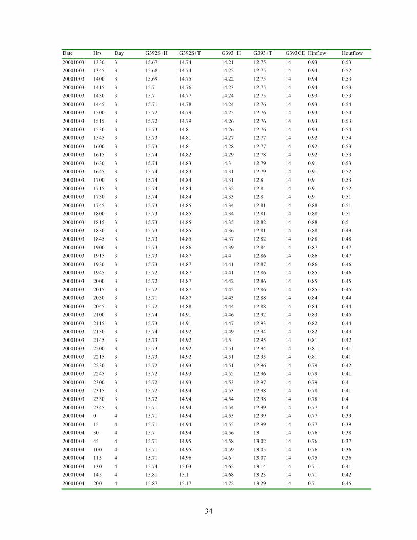
APPENDIX I: STA-6 INFLOW, INTERIOR AND OUTFLOW STAGES FOR OCTOBER 2000 G392S+H = Inflow headwater stage in supply canal (for G601 and G602), G392S+T = Inflow tailwater stage in Cell 3 (for G601 and G602), G393S+H = Outflow headwater stage inside Cell 3 (for G393), G393 +T = Outflow tailwater stage in discharge canal, G393 CE = Weir crest elevation of G393 (weir-culvert combination structure), Hinflow = Head difference across inflow weirs (G601 and G602), Houtflow = Head difference across outflow (G393) Date Hrs Day G392S+H G392S+T G393+H G393+T G393CE Hinflow Houtflow
20001001 0 1 14.41 14.28 14.27 12.82 14 0.13 0.01 20001001 15 1 14.4 14.28 14.26 12.82 14 0.12 0.02 20001001 30 1 14.4 14.28 14.26 12.82 14 0.12 0.02 20001001 45 1 14.39 14.28 14.26 12.82 14 0.11 0.02 20001001 100 1 14.39 14.28 14.26 12.82 14 0.11 0.02 20001001 115 1 14.39 14.28 14.26 12.82 14 0.11 0.02 20001001 130 1 14.38 14.28 14.26 12.82 14 0.1 0.02 20001001 145 1 14.38 14.28 14.26 12.82 14 0.1 0.02 20001001 200 1 14.38 14.27 14.26 12.82 14 0.11 0.01 20001001 215 1 14.37 14.27 14.26 12.82 14 0.1 0.01 20001001 230 1 14.37 14.27 14.25 12.82 14 0.1 0.02 20001001 245 1 14.37 14.27 14.25 12.82 14 0.1 0.02 20001001 300 1 14.37 14.27 14.25 12.82 14 0.1 0.02 20001001 315 1 14.36 14.27 14.25 12.82 14 0.09 0.02 20001001 330 1 14.36 14.27 14.25 12.82 14 0.09 0.02 20001001 345 1 14.36 14.26 14.25 12.82 14 0.1 0.01 20001001 400 1 14.35 14.26 14.25 12.82 14 0.09 0.01 20001001 415 1 14.35 14.26 14.25 12.82 14 0.09 0.01 20001001 430 1 14.35 14.26 14.25 12.82 14 0.09 0.01 20001001 445 1 14.34 14.26 14.24 12.82 14 0.08 0.02 20001001 500 1 14.34 14.26 14.24 12.82 14 0.08 0.02 20001001 515 1 14.34 14.26 14.24 12.82 14 0.08 0.02 20001001 530 1 14.34 14.26 14.24 12.82 14 0.08 0.02 20001001 545 1 14.33 14.26 14.24 12.82 14 0.07 0.02 20001001 600 1 14.33 14.25 14.24 12.82 14 0.08 0.01 20001001 615 1 14.33 14.25 14.24 12.82 14 0.08 0.01 20001001 630 1 14.32 14.25 14.24 12.82 14 0.07 0.01 20001001 645 1 14.32 14.25 14.24 12.82 14 0.07 0.01 20001001 700 1 14.32 14.25 14.23 12.82 14 0.07 0.02 20001001 715 1 14.32 14.25 14.23 12.82 14 0.07 0.02 20001001 730 1 14.31 14.25 14.23 12.82 14 0.06 0.02 20001001 745 1 14.31 14.25 14.23 12.82 14 0.06 0.02 20001001 800 1 14.31 14.24 14.23 12.81 14 0.07 0.01 20001001 815 1 14.48 14.24 14.23 12.81 14 0.24 0.01 20001001 830 1 14.63 14.25 14.23 12.82 14 0.38 0.02 20001001 845 1 14.74 14.26 14.23 12.81 14 0.48 0.03 20001001 900 1 14.83 14.27 14.23 12.81 14 0.56 0.04 20001001 915 1 14.89 14.29 14.23 12.81 14 0.6 0.06 20001001 930 1 14.95 14.31 14.22 12.81 14 0.64 0.09 20001001 945 1 15.02 14.34 14.22 12.81 14 0.68 0.12 20001001 1000 1 15.07 14.36 14.22 12.81 14 0.71 0.14 20001001 1015 1 15.12 14.39 14.22 12.81 14 0.73 0.17

30
Date Hrs Day G392S+H G392S+T G393+H G393+T G393CE Hinflow Houtflow
20001001 1030 1 15.16 14.41 14.22 12.81 14 0.75 0.19 20001001 1045 1 15.21 14.44 14.22 12.81 14 0.77 0.22 20001001 1100 1 15.25 14.46 14.22 12.81 14 0.79 0.24 20001001 1115 1 15.28 14.48 14.22 12.81 14 0.8 0.26 20001001 1130 1 15.31 14.5 14.22 12.8 14 0.81 0.28 20001001 1145 1 15.34 14.52 14.22 12.8 14 0.82 0.3 20001001 1200 1 15.37 14.53 14.22 12.8 14 0.84 0.31 20001001 1215 1 15.39 14.55 14.22 12.8 14 0.84 0.33 20001001 1230 1 15.41 14.56 14.22 12.8 14 0.85 0.34 20001001 1245 1 15.43 14.57 14.22 12.8 14 0.86 0.35 20001001 1300 1 15.44 14.59 14.23 12.8 14 0.85 0.36 20001001 1315 1 15.45 14.6 14.23 12.8 14 0.85 0.37 20001001 1330 1 15.46 14.61 14.23 12.79 14 0.85 0.38 20001001 1345 1 15.47 14.61 14.23 12.79 14 0.86 0.38 20001001 1400 1 15.46 14.62 14.23 12.79 14 0.84 0.39 20001001 1415 1 15.38 14.58 14.24 12.79 14 0.8 0.34 20001001 1430 1 15.3 14.55 14.24 12.79 14 0.75 0.31 20001001 1445 1 15.23 14.52 14.24 12.79 14 0.71 0.28 20001001 1500 1 15.18 14.5 14.24 12.79 14 0.68 0.26 20001001 1515 1 15.14 14.48 14.25 12.79 14 0.66 0.23 20001001 1530 1 15.09 14.46 14.25 12.79 14 0.63 0.21 20001001 1545 1 15.06 14.44 14.25 12.79 14 0.62 0.19 20001001 1600 1 15.02 14.42 14.25 12.79 14 0.6 0.17 20001001 1615 1 14.99 14.41 14.26 12.78 14 0.58 0.15 20001001 1630 1 14.96 14.39 14.26 12.78 14 0.57 0.13 20001001 1645 1 14.93 14.38 14.26 12.78 14 0.55 0.12 20001001 1700 1 14.9 14.37 14.26 12.78 14 0.53 0.11 20001001 1715 1 14.88 14.36 14.26 12.78 14 0.52 0.1 20001001 1730 1 14.85 14.35 14.27 12.78 14 0.5 0.08 20001001 1745 1 14.83 14.35 14.27 12.78 14 0.48 0.08 20001001 1800 1 14.81 14.34 14.27 12.78 14 0.47 0.07 20001001 1815 1 14.79 14.33 14.27 12.78 14 0.46 0.06 20001001 1830 1 14.78 14.33 14.27 12.78 14 0.45 0.06 20001001 1845 1 14.76 14.32 14.27 12.78 14 0.44 0.05 20001001 1900 1 14.74 14.32 14.27 12.78 14 0.42 0.05 20001001 1915 1 14.73 14.32 14.27 12.78 14 0.41 0.05 20001001 1930 1 14.71 14.31 14.27 12.78 14 0.4 0.04 20001001 1945 1 14.7 14.31 14.27 12.78 14 0.39 0.04 20001001 2000 1 14.68 14.31 14.27 12.78 14 0.37 0.04 20001001 2015 1 14.67 14.3 14.27 12.78 14 0.37 0.03 20001001 2030 1 14.66 14.3 14.27 12.78 14 0.36 0.03 20001001 2045 1 14.65 14.3 14.27 12.78 14 0.35 0.03 20001001 2100 1 14.64 14.3 14.27 12.77 14 0.34 0.03 20001001 2115 1 14.63 14.3 14.27 12.78 14 0.33 0.03 20001001 2130 1 14.62 14.29 14.27 12.78 14 0.33 0.02 20001001 2145 1 14.61 14.29 14.27 12.78 14 0.32 0.02 20001001 2200 1 14.6 14.29 14.27 12.78 14 0.31 0.02 20001001 2215 1 14.59 14.29 14.26 12.78 14 0.3 0.03 20001001 2230 1 14.58 14.29 14.26 12.78 14 0.29 0.03 20001001 2245 1 14.57 14.28 14.26 12.77 14 0.29 0.02 20001001 2300 1 14.57 14.28 14.26 12.77 14 0.29 0.02

31
Date Hrs Day G392S+H G392S+T G393+H G393+T G393CE Hinflow Houtflow
20001001 2315 1 14.56 14.28 14.26 12.77 14 0.28 0.02 20001001 2330 1 14.55 14.28 14.26 12.77 14 0.27 0.02 20001001 2345 1 14.54 14.28 14.26 12.77 14 0.26 0.02 20001002 0 2 14.54 14.28 14.26 12.77 14 0.26 0.02 20001002 15 2 14.53 14.28 14.26 12.77 14 0.25 0.02 20001002 30 2 14.52 14.27 14.26 12.77 14 0.25 0.01 20001002 45 2 14.52 14.27 14.25 12.77 14 0.25 0.02 20001002 100 2 14.51 14.27 14.25 12.77 14 0.24 0.02 20001002 115 2 14.5 14.27 14.25 12.77 14 0.23 0.02 20001002 130 2 14.5 14.27 14.25 12.77 14 0.23 0.02 20001002 145 2 14.49 14.27 14.25 12.77 14 0.22 0.02 20001002 200 2 14.49 14.27 14.25 12.77 14 0.22 0.02 20001002 215 2 14.48 14.27 14.25 12.77 14 0.21 0.02 20001002 230 2 14.48 14.26 14.25 12.77 14 0.22 0.01 20001002 245 2 14.47 14.26 14.25 12.77 14 0.21 0.01 20001002 300 2 14.47 14.26 14.25 12.77 14 0.21 0.01 20001002 315 2 14.46 14.26 14.24 12.77 14 0.2 0.02 20001002 330 2 14.46 14.26 14.24 12.77 14 0.2 0.02 20001002 345 2 14.45 14.26 14.24 12.77 14 0.19 0.02 20001002 400 2 14.45 14.26 14.24 12.77 14 0.19 0.02 20001002 415 2 14.44 14.26 14.24 12.77 14 0.18 0.02 20001002 430 2 14.44 14.25 14.24 12.77 14 0.19 0.01 20001002 445 2 14.43 14.25 14.24 12.77 14 0.18 0.01 20001002 500 2 14.43 14.25 14.24 12.77 14 0.18 0.01 20001002 515 2 14.42 14.25 14.24 12.77 14 0.17 0.01 20001002 530 2 14.42 14.25 14.23 12.77 14 0.17 0.02 20001002 545 2 14.42 14.25 14.23 12.77 14 0.17 0.02 20001002 600 2 14.41 14.25 14.23 12.77 14 0.16 0.02 20001002 615 2 14.41 14.25 14.23 12.77 14 0.16 0.02 20001002 630 2 14.4 14.25 14.23 12.77 14 0.15 0.02 20001002 645 2 14.4 14.24 14.23 12.77 14 0.16 0.01 20001002 700 2 14.4 14.24 14.23 12.77 14 0.16 0.01 20001002 715 2 14.39 14.24 14.23 12.77 14 0.15 0.01 20001002 730 2 14.39 14.24 14.23 12.77 14 0.15 0.01 20001002 745 2 14.39 14.24 14.23 12.77 14 0.15 0.01 20001002 800 2 14.38 14.24 14.22 12.77 14 0.14 0.02 20001002 815 2 14.38 14.24 14.22 12.77 14 0.14 0.02 20001002 830 2 14.38 14.24 14.22 12.77 14 0.14 0.02 20001002 845 2 14.37 14.23 14.22 12.77 14 0.14 0.01 20001002 900 2 14.37 14.23 14.22 12.77 14 0.14 0.01 20001002 915 2 14.37 14.23 14.22 12.77 14 0.14 0.01 20001002 930 2 14.36 14.23 14.22 12.77 14 0.13 0.01 20001002 945 2 14.36 14.23 14.22 12.77 14 0.13 0.01 20001002 1000 2 14.36 14.23 14.22 12.77 14 0.13 0.01 20001002 1015 2 14.35 14.23 14.22 12.77 14 0.12 0.01 20001002 1030 2 14.35 14.23 14.21 12.77 14 0.12 0.02 20001002 1045 2 14.35 14.23 14.21 12.77 14 0.12 0.02 20001002 1100 2 14.34 14.23 14.21 12.77 14 0.11 0.02 20001002 1115 2 14.34 14.22 14.21 12.77 14 0.12 0.01 20001002 1130 2 14.34 14.22 14.21 12.77 14 0.12 0.01 20001002 1145 2 14.34 14.22 14.21 12.77 14 0.12 0.01

32
Date Hrs Day G392S+H G392S+T G393+H G393+T G393CE Hinflow Houtflow
20001002 1200 2 14.33 14.22 14.21 12.76 14 0.11 0.01 20001002 1215 2 14.34 14.24 14.22 12.77 14 0.1 0.02 20001002 1230 2 14.34 14.23 14.22 12.76 14 0.11 0.01 20001002 1245 2 14.34 14.23 14.22 12.76 14 0.11 0.01 20001002 1300 2 14.34 14.23 14.21 12.75 14 0.11 0.02 20001002 1315 2 14.34 14.23 14.21 12.75 14 0.11 0.02 20001002 1330 2 14.33 14.23 14.21 12.77 14 0.1 0.02 20001002 1345 2 14.35 14.24 14.21 12.79 14 0.11 0.03 20001002 1400 2 14.35 14.24 14.22 12.79 14 0.11 0.02 20001002 1415 2 14.35 14.24 14.22 12.77 14 0.11 0.02 20001002 1430 2 14.34 14.23 14.22 12.77 14 0.11 0.01 20001002 1445 2 14.34 14.23 14.22 12.76 14 0.11 0.01 20001002 1500 2 14.34 14.23 14.22 12.77 14 0.11 0.01 20001002 1515 2 14.33 14.23 14.22 12.77 14 0.1 0.01 20001002 1530 2 14.33 14.23 14.22 12.78 14 0.1 0.01 20001002 1545 2 14.33 14.23 14.21 12.78 14 0.1 0.02 20001002 1600 2 14.33 14.23 14.21 12.78 14 0.1 0.02 20001002 1615 2 14.33 14.23 14.21 12.79 14 0.1 0.02 20001002 1630 2 14.32 14.22 14.21 12.78 14 0.1 0.01 20001002 1645 2 14.32 14.22 14.21 12.77 14 0.1 0.01 20001002 1700 2 14.32 14.22 14.21 12.77 14 0.1 0.01 20001002 1715 2 14.32 14.22 14.21 12.77 14 0.1 0.01 20001002 1730 2 14.31 14.22 14.21 12.78 14 0.09 0.01 20001002 1745 2 14.31 14.22 14.21 12.78 14 0.09 0.01 20001002 1800 2 14.31 14.22 14.21 12.78 14 0.09 0.01 20001002 1815 2 14.31 14.22 14.21 12.77 14 0.09 0.01 20001002 1830 2 14.3 14.22 14.2 12.77 14 0.08 0.02 20001002 1845 2 14.3 14.21 14.2 12.78 14 0.09 0.01 20001002 1900 2 14.3 14.21 14.2 12.78 14 0.09 0.01 20001002 1915 2 14.3 14.21 14.2 12.78 14 0.09 0.01 20001002 1930 2 14.3 14.21 14.2 12.77 14 0.09 0.01 20001002 1945 2 14.3 14.21 14.2 12.77 14 0.09 0.01 20001002 2000 2 14.3 14.21 14.2 12.77 14 0.09 0.01 20001002 2015 2 14.29 14.21 14.2 12.77 14 0.08 0.01 20001002 2030 2 14.29 14.21 14.2 12.77 14 0.08 0.01 20001002 2045 2 14.29 14.21 14.2 12.77 14 0.08 0.01 20001002 2100 2 14.29 14.21 14.2 12.77 14 0.08 0.01 20001002 2115 2 14.28 14.21 14.2 12.77 14 0.07 0.01 20001002 2130 2 14.28 14.21 14.2 12.77 14 0.07 0.01 20001002 2145 2 14.28 14.21 14.2 12.76 14 0.07 0.01 20001002 2200 2 14.28 14.2 14.2 12.76 14 0.08 0 20001002 2215 2 14.27 14.2 14.19 12.76 14 0.07 0.01 20001002 2230 2 14.27 14.2 14.19 12.76 14 0.07 0.01 20001002 2245 2 14.27 14.2 14.19 12.76 14 0.07 0.01 20001002 2300 2 14.27 14.2 14.19 12.76 14 0.07 0.01 20001002 2315 2 14.27 14.2 14.19 12.76 14 0.07 0.01 20001002 2330 2 14.26 14.2 14.19 12.75 14 0.06 0.01 20001002 2345 2 14.26 14.2 14.19 12.76 14 0.06 0.01 20001003 0 3 14.26 14.2 14.19 12.76 14 0.06 0.01 20001003 15 3 14.26 14.2 14.19 12.76 14 0.06 0.01 20001003 30 3 14.26 14.2 14.19 12.76 14 0.06 0.01

33
Date Hrs Day G392S+H G392S+T G393+H G393+T G393CE Hinflow Houtflow
20001003 45 3 14.25 14.19 14.19 12.76 14 0.06 0 20001003 100 3 14.25 14.19 14.19 12.76 14 0.06 0 20001003 115 3 14.25 14.19 14.19 12.76 14 0.06 0 20001003 130 3 14.25 14.19 14.18 12.76 14 0.06 0.01 20001003 145 3 14.25 14.19 14.18 12.76 14 0.06 0.01 20001003 200 3 14.24 14.19 14.18 12.75 14 0.05 0.01 20001003 215 3 14.24 14.19 14.18 12.75 14 0.05 0.01 20001003 230 3 14.24 14.19 14.18 12.75 14 0.05 0.01 20001003 245 3 14.24 14.19 14.18 12.75 14 0.05 0.01 20001003 300 3 14.23 14.19 14.18 12.75 14 0.04 0.01 20001003 315 3 14.23 14.19 14.18 12.75 14 0.04 0.01 20001003 330 3 14.23 14.19 14.18 12.75 14 0.04 0.01 20001003 345 3 14.23 14.18 14.18 12.75 14 0.05 0 20001003 400 3 14.23 14.18 14.18 12.75 14 0.05 0 20001003 415 3 14.22 14.18 14.18 12.74 14 0.04 0 20001003 430 3 14.22 14.18 14.18 12.74 14 0.04 0 20001003 445 3 14.22 14.18 14.17 12.74 14 0.04 0.01 20001003 500 3 14.22 14.18 14.17 12.74 14 0.04 0.01 20001003 515 3 14.22 14.18 14.17 12.74 14 0.04 0.01 20001003 530 3 14.21 14.18 14.17 12.74 14 0.03 0.01 20001003 545 3 14.21 14.18 14.17 12.74 14 0.03 0.01 20001003 600 3 14.21 14.18 14.17 12.74 14 0.03 0.01 20001003 615 3 14.21 14.18 14.17 12.74 14 0.03 0.01 20001003 630 3 14.21 14.18 14.17 12.74 14 0.03 0.01 20001003 645 3 14.2 14.18 14.17 12.74 14 0.02 0.01 20001003 700 3 14.2 14.17 14.17 12.74 14 0.03 0 20001003 715 3 14.2 14.17 14.17 12.74 14 0.03 0 20001003 730 3 14.2 14.17 14.17 12.74 14 0.03 0 20001003 745 3 14.43 14.17 14.17 12.74 14 0.26 0 20001003 800 3 14.64 14.18 14.17 12.73 14 0.46 0.01 20001003 815 3 14.79 14.21 14.17 12.73 14 0.58 0.04 20001003 830 3 14.92 14.24 14.17 12.73 14 0.68 0.07 20001003 845 3 15 14.28 14.17 12.73 14 0.72 0.11 20001003 900 3 15.08 14.32 14.17 12.73 14 0.76 0.15 20001003 915 3 15.14 14.36 14.16 12.73 14 0.78 0.2 20001003 930 3 15.2 14.4 14.16 12.73 14 0.8 0.24 20001003 945 3 15.27 14.43 14.16 12.73 14 0.84 0.27 20001003 1000 3 15.32 14.47 14.16 12.73 14 0.85 0.31 20001003 1015 3 15.37 14.5 14.17 12.72 14 0.87 0.33 20001003 1030 3 15.42 14.53 14.17 12.72 14 0.89 0.36 20001003 1045 3 15.45 14.56 14.17 12.73 14 0.89 0.39 20001003 1100 3 15.49 14.58 14.17 12.73 14 0.91 0.41 20001003 1115 3 15.52 14.61 14.18 12.74 14 0.91 0.43 20001003 1130 3 15.55 14.63 14.18 12.74 14 0.92 0.45 20001003 1145 3 15.58 14.65 14.18 12.74 14 0.93 0.47 20001003 1200 3 15.59 14.66 14.18 12.73 14 0.93 0.48 20001003 1215 3 15.61 14.67 14.19 12.72 14 0.94 0.48 20001003 1230 3 15.63 14.69 14.19 12.72 14 0.94 0.5 20001003 1245 3 15.64 14.7 14.19 12.72 14 0.94 0.51 20001003 1300 3 15.65 14.71 14.2 12.73 14 0.94 0.51 20001003 1315 3 15.66 14.73 14.21 12.74 14 0.93 0.52
34
Date Hrs Day G392S+H G392S+T G393+H G393+T G393CE Hinflow Houtflow
20001003 1330 3 15.67 14.74 14.21 12.75 14 0.93 0.53 20001003 1345 3 15.68 14.74 14.22 12.75 14 0.94 0.52 20001003 1400 3 15.69 14.75 14.22 12.75 14 0.94 0.53 20001003 1415 3 15.7 14.76 14.23 12.75 14 0.94 0.53 20001003 1430 3 15.7 14.77 14.24 12.75 14 0.93 0.53 20001003 1445 3 15.71 14.78 14.24 12.76 14 0.93 0.54 20001003 1500 3 15.72 14.79 14.25 12.76 14 0.93 0.54 20001003 1515 3 15.72 14.79 14.26 12.76 14 0.93 0.53 20001003 1530 3 15.73 14.8 14.26 12.76 14 0.93 0.54 20001003 1545 3 15.73 14.81 14.27 12.77 14 0.92 0.54 20001003 1600 3 15.73 14.81 14.28 12.77 14 0.92 0.53 20001003 1615 3 15.74 14.82 14.29 12.78 14 0.92 0.53 20001003 1630 3 15.74 14.83 14.3 12.79 14 0.91 0.53 20001003 1645 3 15.74 14.83 14.31 12.79 14 0.91 0.52 20001003 1700 3 15.74 14.84 14.31 12.8 14 0.9 0.53 20001003 1715 3 15.74 14.84 14.32 12.8 14 0.9 0.52 20001003 1730 3 15.74 14.84 14.33 12.8 14 0.9 0.51 20001003 1745 3 15.73 14.85 14.34 12.81 14 0.88 0.51 20001003 1800 3 15.73 14.85 14.34 12.81 14 0.88 0.51 20001003 1815 3 15.73 14.85 14.35 12.82 14 0.88 0.5 20001003 1830 3 15.73 14.85 14.36 12.81 14 0.88 0.49 20001003 1845 3 15.73 14.85 14.37 12.82 14 0.88 0.48 20001003 1900 3 15.73 14.86 14.39 12.84 14 0.87 0.47 20001003 1915 3 15.73 14.87 14.4 12.86 14 0.86 0.47 20001003 1930 3 15.73 14.87 14.41 12.87 14 0.86 0.46 20001003 1945 3 15.72 14.87 14.41 12.86 14 0.85 0.46 20001003 2000 3 15.72 14.87 14.42 12.86 14 0.85 0.45 20001003 2015 3 15.72 14.87 14.42 12.86 14 0.85 0.45 20001003 2030 3 15.71 14.87 14.43 12.88 14 0.84 0.44 20001003 2045 3 15.72 14.88 14.44 12.88 14 0.84 0.44 20001003 2100 3 15.74 14.91 14.46 12.92 14 0.83 0.45 20001003 2115 3 15.73 14.91 14.47 12.93 14 0.82 0.44 20001003 2130 3 15.74 14.92 14.49 12.94 14 0.82 0.43 20001003 2145 3 15.73 14.92 14.5 12.95 14 0.81 0.42 20001003 2200 3 15.73 14.92 14.51 12.94 14 0.81 0.41 20001003 2215 3 15.73 14.92 14.51 12.95 14 0.81 0.41 20001003 2230 3 15.72 14.93 14.51 12.96 14 0.79 0.42 20001003 2245 3 15.72 14.93 14.52 12.96 14 0.79 0.41 20001003 2300 3 15.72 14.93 14.53 12.97 14 0.79 0.4 20001003 2315 3 15.72 14.94 14.53 12.98 14 0.78 0.41 20001003 2330 3 15.72 14.94 14.54 12.98 14 0.78 0.4 20001003 2345 3 15.71 14.94 14.54 12.99 14 0.77 0.4 20001004 0 4 15.71 14.94 14.55 12.99 14 0.77 0.39 20001004 15 4 15.71 14.94 14.55 12.99 14 0.77 0.39 20001004 30 4 15.7 14.94 14.56 13 14 0.76 0.38 20001004 45 4 15.71 14.95 14.58 13.02 14 0.76 0.37 20001004 100 4 15.71 14.95 14.59 13.05 14 0.76 0.36 20001004 115 4 15.71 14.96 14.6 13.07 14 0.75 0.36 20001004 130 4 15.74 15.03 14.62 13.14 14 0.71 0.41 20001004 145 4 15.81 15.1 14.68 13.23 14 0.71 0.42 20001004 200 4 15.87 15.17 14.72 13.29 14 0.7 0.45

35
Date Hrs Day G392S+H G392S+T G393+H G393+T G393CE Hinflow Houtflow
20001004 215 4 15.88 15.18 14.74 13.3 14 0.7 0.44 20001004 230 4 15.93 15.26 14.81 13.36 14 0.67 0.45 20001004 245 4 15.93 15.29 14.85 13.41 14 0.64 0.44 20001004 300 4 15.95 15.33 14.87 13.46 14 0.62 0.46 20001004 315 4 15.96 15.35 14.89 13.49 14 0.61 0.46 20001004 330 4 15.97 15.38 14.92 13.52 14 0.59 0.46 20001004 345 4 16.03 15.43 14.96 13.61 14 0.6 0.47 20001004 400 4 16.05 15.47 15.03 13.71 14 0.58 0.44 20001004 415 4 16.03 15.48 15.05 13.78 14 0.55 0.43 20001004 430 4 16.06 15.54 15.09 13.83 14 0.52 0.45 20001004 445 4 16.12 15.62 15.16 13.94 14 0.5 0.46 20001004 500 4 16.15 15.68 15.25 14.05 14 0.47 0.43 20001004 515 4 16.14 15.7 15.31 14.11 14 0.44 0.39 20001004 530 4 16.14 15.73 15.36 14.17 14 0.41 0.37 20001004 545 4 16.12 15.74 15.37 14.2 14 0.38 0.37 20001004 600 4 16.13 15.79 15.42 14.24 14 0.34 0.37 20001004 615 4 16.12 15.8 15.44 14.28 14 0.32 0.36 20001004 630 4 16.1 15.81 15.46 14.29 14 0.29 0.35 20001004 645 4 16.08 15.81 15.47 14.3 14 0.27 0.34 20001004 700 4 16.07 15.81 15.48 14.31 14 0.26 0.33 20001004 715 4 16.07 15.83 15.51 14.33 14 0.24 0.32 20001004 730 4 16.05 15.83 15.51 14.34 14 0.22 0.32 20001004 745 4 16.04 15.83 15.52 14.34 14 0.21 0.31 20001004 800 4 16.06 15.86 15.52 14.35 14 0.2 0.34 20001004 815 4 16.06 15.87 15.55 14.39 14 0.19 0.32 20001004 830 4 16.07 15.88 15.56 14.4 14 0.19 0.32 20001004 845 4 16.06 15.88 15.58 14.4 14 0.18 0.3 20001004 900 4 16.1 15.93 15.61 14.44 14 0.17 0.32 20001004 915 4 16.13 15.97 15.65 14.49 14 0.16 0.32 20001004 930 4 16.14 16 15.68 14.52 14 0.14 0.32 20001004 945 4 16.15 16.01 15.7 14.54 14 0.14 0.31 20001004 1000 4 16.14 16.01 15.71 14.54 14 0.13 0.3 20001004 1015 4 16.13 16.01 15.72 14.54 14 0.12 0.29 20001004 1030 4 16.12 16 15.73 14.53 14 0.12 0.27 20001004 1045 4 16.11 15.99 15.73 14.53 14 0.12 0.26 20001004 1100 4 16.09 15.99 15.73 14.52 14 0.1 0.26 20001004 1115 4 16.09 15.99 15.73 14.52 14 0.1 0.26 20001004 1130 4 16.09 15.98 15.73 14.51 14 0.11 0.25 20001004 1145 4 16.09 15.99 15.73 14.51 14 0.1 0.26 20001004 1200 4 16.09 15.99 15.73 14.5 14 0.1 0.26 20001004 1215 4 16.08 15.98 15.73 14.5 14 0.1 0.25 20001004 1230 4 16.08 15.98 15.73 14.49 14 0.1 0.25 20001004 1245 4 16.07 15.98 15.73 14.48 14 0.09 0.25 20001004 1300 4 16.07 15.97 15.73 14.47 14 0.1 0.24 20001004 1315 4 16.07 15.97 15.73 14.47 14 0.1 0.24 20001004 1330 4 16.06 15.97 15.73 14.46 14 0.09 0.24 20001004 1345 4 16.06 15.97 15.72 14.46 14 0.09 0.25 20001004 1400 4 16.06 15.96 15.72 14.45 14 0.1 0.24 20001004 1415 4 16.06 15.96 15.72 14.44 14 0.1 0.24 20001004 1430 4 16.05 15.96 15.71 14.44 14 0.09 0.25 20001004 1445 4 16.05 15.96 15.71 14.43 14 0.09 0.25

36
Date Hrs Day G392S+H G392S+T G393+H G393+T G393CE Hinflow Houtflow
20001004 1500 4 16.05 15.95 15.71 14.42 14 0.1 0.24 20001004 1515 4 16.05 15.95 15.7 14.42 14 0.1 0.25 20001004 1530 4 16.05 15.95 15.7 14.41 14 0.1 0.25 20001004 1545 4 16.05 15.95 15.7 14.41 14 0.1 0.25 20001004 1600 4 16.05 15.95 15.7 14.41 14 0.1 0.25 20001004 1615 4 16.05 15.94 15.69 14.4 14 0.11 0.25 20001004 1630 4 16.05 15.94 15.69 14.4 14 0.11 0.25 20001004 1645 4 16.03 15.93 15.69 14.4 14 0.1 0.24 20001004 1700 4 16.03 15.93 15.69 14.4 14 0.1 0.24 20001004 1715 4 16.05 15.94 15.69 14.39 14 0.11 0.25 20001004 1730 4 16.05 15.94 15.68 14.39 14 0.11 0.26 20001004 1745 4 16.05 15.94 15.68 14.39 14 0.11 0.26 20001004 1800 4 16.05 15.94 15.68 14.4 14 0.11 0.26 20001004 1815 4 16.05 15.93 15.68 14.4 14 0.12 0.25 20001004 1830 4 16.05 15.93 15.67 14.4 14 0.12 0.26 20001004 1845 4 16.05 15.93 15.67 14.4 14 0.12 0.26 20001004 1900 4 16.05 15.93 15.67 14.4 14 0.12 0.26 20001004 1915 4 16.05 15.93 15.67 14.4 14 0.12 0.26 20001004 1930 4 16.05 15.93 15.67 14.4 14 0.12 0.26 20001004 1945 4 16.05 15.93 15.67 14.41 14 0.12 0.26 20001004 2000 4 16.05 15.93 15.66 14.41 14 0.12 0.27 20001004 2015 4 16.05 15.93 15.66 14.41 14 0.12 0.27 20001004 2030 4 16.05 15.92 15.66 14.42 14 0.13 0.26 20001004 2045 4 16.05 15.92 15.66 14.42 14 0.13 0.26 20001004 2100 4 16.04 15.92 15.66 14.42 14 0.12 0.26 20001004 2115 4 16.04 15.92 15.66 14.42 14 0.12 0.26 20001004 2130 4 16.04 15.92 15.66 14.42 14 0.12 0.26 20001004 2145 4 16.04 15.92 15.66 14.42 14 0.12 0.26 20001004 2200 4 16.04 15.92 15.65 14.42 14 0.12 0.27 20001004 2215 4 16.04 15.91 15.65 14.42 14 0.13 0.26 20001004 2230 4 16.04 15.91 15.65 14.42 14 0.13 0.26 20001004 2245 4 16.04 15.91 15.65 14.42 14 0.13 0.26 20001004 2300 4 16.04 15.91 15.65 14.42 14 0.13 0.26 20001004 2315 4 16.04 15.91 15.65 14.42 14 0.13 0.26 20001004 2330 4 16.03 15.91 15.65 14.42 14 0.12 0.26 20001004 2345 4 16.03 15.91 15.65 14.42 14 0.12 0.26 20001005 0 16.03 15.9 15.64 14.42 14 0.13 0.26 20001005 15 5 16.03 15.9 15.64 14.42 14 0.13 0.26 20001005 30 5 16.03 15.9 15.64 14.42 14 0.13 0.26 20001005 45 5 16.03 15.9 15.64 14.42 14 0.13 0.26 20001005 100 5 16.03 15.9 15.64 14.42 14 0.13 0.26 20001005 115 5 16.03 15.9 15.64 14.42 14 0.13 0.26 20001005 130 5 16.03 15.9 15.64 14.41 14 0.13 0.26 20001005 145 5 16.03 15.9 15.63 14.41 14 0.13 0.27 20001005 200 5 16.03 15.89 15.63 14.41 14 0.14 0.26 20001005 215 5 16.03 15.89 15.63 14.41 14 0.14 0.26 20001005 230 5 16.02 15.89 15.63 14.41 14 0.13 0.26 20001005 245 5 16.02 15.89 15.63 14.41 14 0.13 0.26 20001005 300 5 16.02 15.89 15.63 14.41 14 0.13 0.26 20001005 315 5 16.02 15.89 15.63 14.41 14 0.13 0.26 20001005 330 5 16.02 15.89 15.63 14.41 14 0.13 0.26

37
Date Hrs Day G392S+H G392S+T G393+H G393+T G393CE Hinflow Houtflow
20001005 345 5 16.02 15.89 15.62 14.41 14 0.13 0.27 20001005 400 5 16.02 15.89 15.62 14.41 14 0.13 0.27 20001005 415 5 16.02 15.88 15.62 14.41 14 0.14 0.26 20001005 430 5 16.02 15.88 15.62 14.4 14 0.14 0.26 20001005 445 5 16.02 15.88 15.62 14.4 14 0.14 0.26 20001005 500 5 16.02 15.88 15.62 14.4 14 0.14 0.26 20001005 515 5 16.02 15.88 15.62 14.4 14 0.14 0.26 20001005 530 5 16.01 15.88 15.61 14.4 14 0.13 0.27 20001005 545 5 16.01 15.88 15.61 14.4 14 0.13 0.27 20001005 600 5 16.01 15.88 15.61 14.4 14 0.13 0.27 20001005 615 5 16.01 15.88 15.61 14.4 14 0.13 0.27 20001005 630 5 16.01 15.88 15.61 14.4 14 0.13 0.27 20001005 645 5 16.01 15.88 15.61 14.39 14 0.13 0.27 20001005 700 5 16.01 15.87 15.61 14.39 14 0.14 0.26 20001005 715 5 16.01 15.87 15.61 14.39 14 0.14 0.26 20001005 730 5 16.01 15.87 15.6 14.39 14 0.14 0.27 20001005 745 5 16.01 15.87 15.6 14.39 14 0.14 0.27 20001005 800 5 16.01 15.87 15.6 14.39 14 0.14 0.27 20001005 815 5 16.01 15.87 15.6 14.39 14 0.14 0.27 20001005 830 5 16.01 15.87 15.6 14.39 14 0.14 0.27 20001005 845 5 16.01 15.87 15.6 14.39 14 0.14 0.27 20001005 900 5 16.01 15.87 15.6 14.39 14 0.14 0.27 20001005 915 5 16.01 15.87 15.6 14.38 14 0.14 0.27 20001005 930 5 16 15.86 15.6 14.38 14 0.14 0.26 20001005 945 5 16 15.86 15.6 14.38 14 0.14 0.26 20001005 1000 5 16 15.86 15.59 14.38 14 0.14 0.27 20001005 1015 5 16 15.86 15.59 14.38 14 0.14 0.27 20001005 1030 5 16 15.86 15.59 14.37 14 0.14 0.27 20001005 1045 5 16 15.86 15.59 14.37 14 0.14 0.27 20001005 1100 5 16 15.86 15.59 14.37 14 0.14 0.27 20001005 1115 5 16 15.86 15.59 14.36 14 0.14 0.27 20001005 1130 5 15.97 15.85 15.59 14.35 14 0.12 0.26 20001005 1145 5 15.99 15.85 15.59 14.35 14 0.14 0.26 20001005 1200 5 16 15.85 15.58 14.34 14 0.15 0.27 20001005 1215 5 15.99 15.85 15.58 14.33 14 0.14 0.27 20001005 1230 5 15.99 15.85 15.58 14.32 14 0.14 0.27 20001005 1245 5 15.99 15.85 15.58 14.31 14 0.14 0.27 20001005 1300 5 15.99 15.85 15.58 14.31 14 0.14 0.27 20001005 1315 5 15.99 15.85 15.58 14.3 14 0.14 0.27 20001005 1330 5 15.99 15.85 15.57 14.29 14 0.14 0.28 20001005 1345 5 15.99 15.85 15.57 14.29 14 0.14 0.28 20001005 1400 5 15.99 15.85 15.57 14.28 14 0.14 0.28 20001005 1415 5 15.99 15.84 15.57 14.28 14 0.15 0.27 20001005 1430 5 15.99 15.84 15.57 14.27 14 0.15 0.27 20001005 1445 5 15.99 15.84 15.57 14.27 14 0.15 0.27 20001005 1500 5 15.99 15.84 15.56 14.27 14 0.15 0.28 20001005 1515 5 15.99 15.84 15.56 14.27 14 0.15 0.28 20001005 1530 5 15.99 15.84 15.56 14.26 14 0.15 0.28 20001005 1545 5 15.99 15.84 15.56 14.26 14 0.15 0.28 20001005 1600 5 15.99 15.84 15.56 14.25 14 0.15 0.28 20001005 1615 5 15.99 15.84 15.56 14.25 14 0.15 0.28

38
Date Hrs Day G392S+H G392S+T G393+H G393+T G393CE Hinflow Houtflow
20001005 1630 5 15.99 15.84 15.55 14.24 14 0.15 0.29 20001005 1645 5 15.99 15.83 15.55 14.24 14 0.16 0.28 20001005 1700 5 15.99 15.83 15.55 14.24 14 0.16 0.28 20001005 1715 5 15.96 15.83 15.55 14.24 14 0.13 0.28 20001005 1730 5 15.97 15.83 15.55 14.23 14 0.14 0.28 20001005 1745 5 15.97 15.82 15.55 14.23 14 0.15 0.27 20001005 1800 5 15.97 15.82 15.55 14.23 14 0.15 0.27 20001005 1815 5 15.86 15.8 15.54 14.23 14 0.06 0.26 20001005 1830 5 15.97 15.82 15.54 14.22 14 0.15 0.28 20001005 1845 5 16.01 15.82 15.54 14.22 14 0.19 0.28 20001005 1900 5 16.01 15.83 15.54 14.22 14 0.18 0.29 20001005 1915 5 16.03 15.83 15.54 14.22 14 0.2 0.29 20001005 1930 5 16.05 15.84 15.54 14.22 14 0.21 0.3 20001005 1945 5 16.06 15.85 15.54 14.22 14 0.21 0.31 20001005 2000 5 16.07 15.85 15.54 14.21 14 0.22 0.31 20001005 2015 5 16.08 15.85 15.54 14.21 14 0.23 0.31 20001005 2030 5 16.08 15.86 15.54 14.21 14 0.22 0.32 20001005 2045 5 16.09 15.86 15.54 14.21 14 0.23 0.32 20001005 2100 5 16.09 15.86 15.54 14.21 14 0.23 0.32 20001005 2115 5 16.09 15.87 15.54 14.21 14 0.22 0.33 20001005 2130 5 16.1 15.87 15.54 14.21 14 0.23 0.33 20001005 2145 5 16.1 15.87 15.54 14.2 14 0.23 0.33 20001005 2200 5 16.1 15.87 15.54 14.2 14 0.23 0.33 20001005 2215 5 16.09 15.87 15.54 14.2 14 0.22 0.33 20001005 2230 5 16.09 15.87 15.54 14.2 14 0.22 0.33 20001005 2245 5 16.09 15.87 15.54 14.2 14 0.22 0.33 20001005 2300 5 16.09 15.87 15.54 14.2 14 0.22 0.33 20001005 2315 5 16.09 15.87 15.54 14.2 14 0.22 0.33 20001005 2330 5 16.09 15.87 15.55 14.2 14 0.22 0.32 20001005 2345 5 16.09 15.87 15.55 14.19 14 0.22 0.32 20001006 0 6 16.09 15.87 15.55 14.2 14 0.22 0.32 20001006 15 6 16.09 15.87 15.55 14.19 14 0.22 0.32 20001006 30 6 16.09 15.88 15.55 14.19 14 0.21 0.33 20001006 45 6 16.09 15.88 15.55 14.19 14 0.21 0.33 20001006 100 6 16.09 15.88 15.55 14.19 14 0.21 0.33 20001006 115 6 16.09 15.88 15.55 14.19 14 0.21 0.33 20001006 130 6 16.09 15.88 15.55 14.19 14 0.21 0.33 20001006 145 6 16.09 15.88 15.55 14.19 14 0.21 0.33 20001006 200 6 16.09 15.88 15.55 14.19 14 0.21 0.33 20001006 215 6 16.09 15.88 15.56 14.19 14 0.21 0.32 20001006 230 6 16.09 15.88 15.56 14.19 14 0.21 0.32 20001006 245 6 16.09 15.88 15.56 14.19 14 0.21 0.32 20001006 300 6 16.09 15.88 15.56 14.19 14 0.21 0.32 20001006 315 6 16.08 15.88 15.56 14.19 14 0.2 0.32 20001006 330 6 16.09 15.88 15.56 14.19 14 0.21 0.32 20001006 345 6 16.08 15.88 15.56 14.19 14 0.2 0.32 20001006 400 6 16.09 15.88 15.56 14.19 14 0.21 0.32 20001006 415 6 16.09 15.88 15.56 14.19 14 0.21 0.32 20001006 430 6 16.09 15.89 15.56 14.19 14 0.2 0.33 20001006 445 6 16.09 15.89 15.56 14.18 14 0.2 0.33 20001006 500 6 16.09 15.89 15.56 14.18 14 0.2 0.33

39
Date Hrs Day G392S+H G392S+T G393+H G393+T G393CE Hinflow Houtflow
20001006 515 6 16.09 15.89 15.56 14.18 14 0.2 0.33 20001006 530 6 16.09 15.89 15.56 14.18 14 0.2 0.33 20001006 545 6 16.09 15.89 15.56 14.18 14 0.2 0.33 20001006 600 6 16.09 15.89 15.56 14.18 14 0.2 0.33 20001006 615 6 16.09 15.89 15.57 14.18 14 0.2 0.32 20001006 630 6 16.09 15.89 15.57 14.18 14 0.2 0.32 20001006 645 6 16.09 15.89 15.57 14.18 14 0.2 0.32 20001006 700 6 16.09 15.89 15.57 14.18 14 0.2 0.32 20001006 715 6 16.09 15.89 15.57 14.18 14 0.2 0.32 20001006 730 6 16.09 15.89 15.57 14.18 14 0.2 0.32 20001006 745 6 16.09 15.89 15.57 14.18 14 0.2 0.32 20001006 800 6 16.09 15.89 15.57 14.18 14 0.2 0.32 20001006 815 6 16.09 15.9 15.57 14.18 14 0.19 0.33 20001006 830 6 16.09 15.9 15.57 14.18 14 0.19 0.33 20001006 845 6 16.09 15.9 15.57 14.18 14 0.19 0.33 20001006 900 6 16.09 15.9 15.57 14.18 14 0.19 0.33 20001006 915 6 16.09 15.9 15.57 14.18 14 0.19 0.33 20001006 930 6 16.08 15.9 15.57 14.18 14 0.18 0.33 20001006 945 6 16.08 15.9 15.57 14.18 14 0.18 0.33 20001006 1000 6 16.07 15.89 15.57 14.17 14 0.18 0.32 20001006 1015 6 16.08 15.9 15.57 14.17 14 0.18 0.33 20001006 1030 6 16.09 15.9 15.57 14.17 14 0.19 0.33 20001006 1045 6 16.09 15.9 15.57 14.17 14 0.19 0.33 20001006 1100 6 16.09 15.9 15.57 14.17 14 0.19 0.33 20001006 1115 6 16.1 15.9 15.57 14.17 14 0.2 0.33 20001006 1130 6 16.1 15.9 15.57 14.17 14 0.2 0.33 20001006 1145 6 16.1 15.9 15.57 14.17 14 0.2 0.33 20001006 1200 6 16.1 15.9 15.57 14.17 14 0.2 0.33 20001006 1215 6 16.1 15.91 15.57 14.16 14 0.19 0.34 20001006 1230 6 16.1 15.91 15.57 14.16 14 0.19 0.34 20001006 1245 6 16.1 15.91 15.57 14.16 14 0.19 0.34 20001006 1300 6 16.1 15.91 15.57 14.16 14 0.19 0.34 20001006 1315 6 16.1 15.91 15.58 14.16 14 0.19 0.33 20001006 1330 6 16.1 15.91 15.58 14.16 14 0.19 0.33 20001006 1345 6 16.1 15.91 15.58 14.16 14 0.19 0.33 20001006 1400 6 16.07 15.9 15.58 14.16 14 0.17 0.32 20001006 1415 6 16.06 15.89 15.58 14.16 14 0.17 0.31 20001006 1430 6 16.01 15.88 15.58 14.16 14 0.13 0.3 20001006 1445 6 16.02 15.88 15.58 14.16 14 0.14 0.3 20001006 1500 6 16.06 15.88 15.58 14.16 14 0.18 0.3 20001006 1515 6 16.05 15.88 15.58 14.15 14 0.17 0.3 20001006 1530 6 16.06 15.88 15.57 14.15 14 0.18 0.31 20001006 1545 6 16.06 15.89 15.57 14.15 14 0.17 0.32 20001006 1600 6 16.06 15.89 15.57 14.15 14 0.17 0.32 20001006 1615 6 16.07 15.89 15.58 14.16 14 0.18 0.31 20001006 1630 6 16.06 15.89 15.57 14.16 14 0.17 0.32 20001006 1645 6 16.07 15.89 15.57 14.16 14 0.18 0.32 20001006 1700 6 16.05 15.89 15.57 14.16 14 0.16 0.32 20001006 1715 6 16.05 15.89 15.57 14.16 14 0.16 0.32 20001006 1730 6 16.06 15.89 15.57 14.16 14 0.17 0.32 20001006 1745 6 16.11 15.93 15.58 14.19 14 0.18 0.35
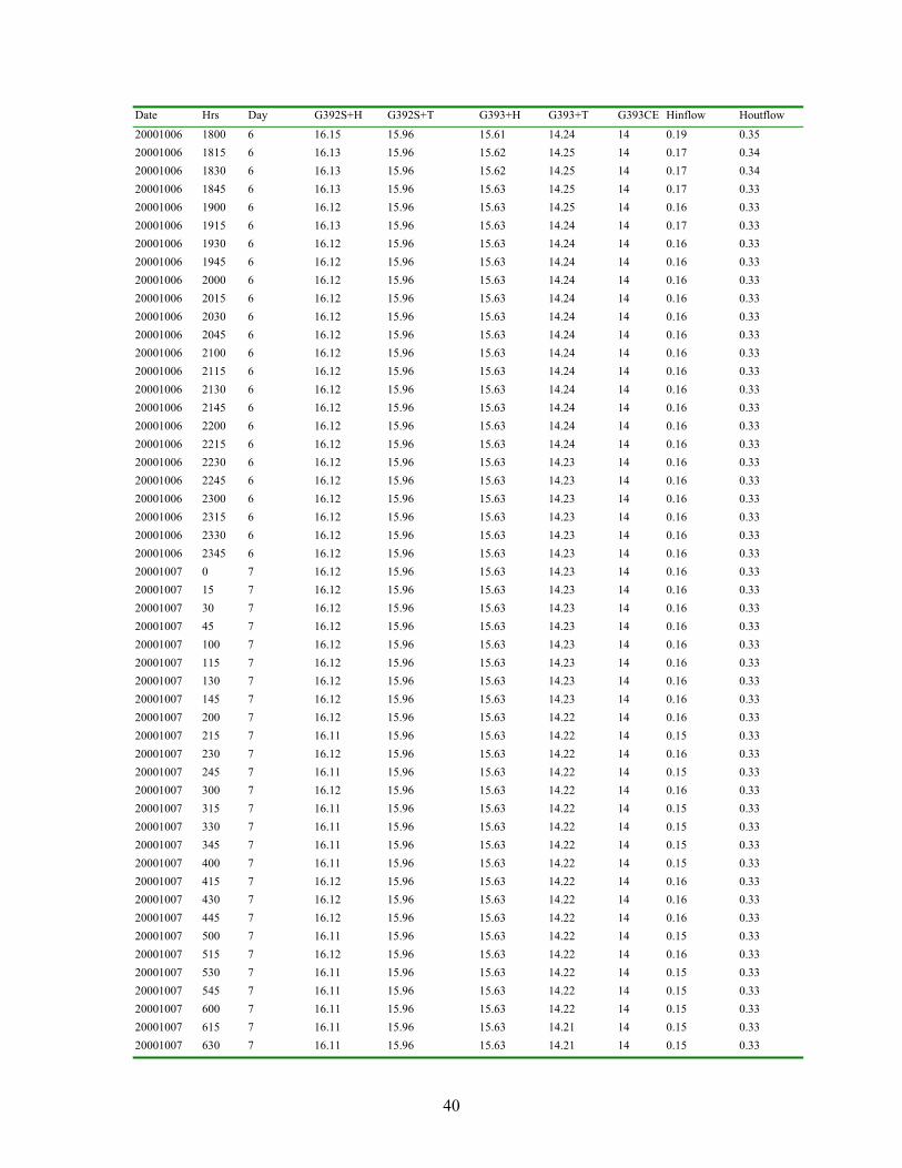
40
Date Hrs Day G392S+H G392S+T G393+H G393+T G393CE Hinflow Houtflow
20001006 1800 6 16.15 15.96 15.61 14.24 14 0.19 0.35 20001006 1815 6 16.13 15.96 15.62 14.25 14 0.17 0.34 20001006 1830 6 16.13 15.96 15.62 14.25 14 0.17 0.34 20001006 1845 6 16.13 15.96 15.63 14.25 14 0.17 0.33 20001006 1900 6 16.12 15.96 15.63 14.25 14 0.16 0.33 20001006 1915 6 16.13 15.96 15.63 14.24 14 0.17 0.33 20001006 1930 6 16.12 15.96 15.63 14.24 14 0.16 0.33 20001006 1945 6 16.12 15.96 15.63 14.24 14 0.16 0.33 20001006 2000 6 16.12 15.96 15.63 14.24 14 0.16 0.33 20001006 2015 6 16.12 15.96 15.63 14.24 14 0.16 0.33 20001006 2030 6 16.12 15.96 15.63 14.24 14 0.16 0.33 20001006 2045 6 16.12 15.96 15.63 14.24 14 0.16 0.33 20001006 2100 6 16.12 15.96 15.63 14.24 14 0.16 0.33 20001006 2115 6 16.12 15.96 15.63 14.24 14 0.16 0.33 20001006 2130 6 16.12 15.96 15.63 14.24 14 0.16 0.33 20001006 2145 6 16.12 15.96 15.63 14.24 14 0.16 0.33 20001006 2200 6 16.12 15.96 15.63 14.24 14 0.16 0.33 20001006 2215 6 16.12 15.96 15.63 14.24 14 0.16 0.33 20001006 2230 6 16.12 15.96 15.63 14.23 14 0.16 0.33 20001006 2245 6 16.12 15.96 15.63 14.23 14 0.16 0.33 20001006 2300 6 16.12 15.96 15.63 14.23 14 0.16 0.33 20001006 2315 6 16.12 15.96 15.63 14.23 14 0.16 0.33 20001006 2330 6 16.12 15.96 15.63 14.23 14 0.16 0.33 20001006 2345 6 16.12 15.96 15.63 14.23 14 0.16 0.33 20001007 0 7 16.12 15.96 15.63 14.23 14 0.16 0.33 20001007 15 7 16.12 15.96 15.63 14.23 14 0.16 0.33 20001007 30 7 16.12 15.96 15.63 14.23 14 0.16 0.33 20001007 45 7 16.12 15.96 15.63 14.23 14 0.16 0.33 20001007 100 7 16.12 15.96 15.63 14.23 14 0.16 0.33 20001007 115 7 16.12 15.96 15.63 14.23 14 0.16 0.33 20001007 130 7 16.12 15.96 15.63 14.23 14 0.16 0.33 20001007 145 7 16.12 15.96 15.63 14.23 14 0.16 0.33 20001007 200 7 16.12 15.96 15.63 14.22 14 0.16 0.33 20001007 215 7 16.11 15.96 15.63 14.22 14 0.15 0.33 20001007 230 7 16.12 15.96 15.63 14.22 14 0.16 0.33 20001007 245 7 16.11 15.96 15.63 14.22 14 0.15 0.33 20001007 300 7 16.12 15.96 15.63 14.22 14 0.16 0.33 20001007 315 7 16.11 15.96 15.63 14.22 14 0.15 0.33 20001007 330 7 16.11 15.96 15.63 14.22 14 0.15 0.33 20001007 345 7 16.11 15.96 15.63 14.22 14 0.15 0.33 20001007 400 7 16.11 15.96 15.63 14.22 14 0.15 0.33 20001007 415 7 16.12 15.96 15.63 14.22 14 0.16 0.33 20001007 430 7 16.12 15.96 15.63 14.22 14 0.16 0.33 20001007 445 7 16.12 15.96 15.63 14.22 14 0.16 0.33 20001007 500 7 16.11 15.96 15.63 14.22 14 0.15 0.33 20001007 515 7 16.12 15.96 15.63 14.22 14 0.16 0.33 20001007 530 7 16.11 15.96 15.63 14.22 14 0.15 0.33 20001007 545 7 16.11 15.96 15.63 14.22 14 0.15 0.33 20001007 600 7 16.11 15.96 15.63 14.22 14 0.15 0.33 20001007 615 7 16.11 15.96 15.63 14.21 14 0.15 0.33 20001007 630 7 16.11 15.96 15.63 14.21 14 0.15 0.33

41
Date Hrs Day G392S+H G392S+T G393+H G393+T G393CE Hinflow Houtflow
20001007 645 7 16.11 15.96 15.63 14.21 14 0.15 0.33 20001007 700 7 16.11 15.96 15.63 14.21 14 0.15 0.33 20001007 715 7 16.11 15.96 15.63 14.21 14 0.15 0.33 20001007 730 7 16.12 15.96 15.63 14.21 14 0.16 0.33 20001007 745 7 16.12 15.96 15.63 14.21 14 0.16 0.33 20001007 800 7 16.12 15.96 15.63 14.21 14 0.16 0.33 20001007 815 7 16.12 15.96 15.63 14.21 14 0.16 0.33 20001007 830 7 16.12 15.96 15.63 14.21 14 0.16 0.33 20001007 845 7 16.12 15.96 15.63 14.21 14 0.16 0.33 20001007 900 7 16.12 15.96 15.63 14.21 14 0.16 0.33 20001007 915 7 16.11 15.96 15.63 14.21 14 0.15 0.33 20001007 930 7 16.12 15.96 15.63 14.21 14 0.16 0.33 20001007 945 7 16.12 15.96 15.63 14.21 14 0.16 0.33 20001007 1000 7 16.1 15.96 15.63 14.2 14 0.14 0.33 20001007 1015 7 16.12 15.96 15.63 14.2 14 0.16 0.33 20001007 1030 7 16.12 15.96 15.63 14.2 14 0.16 0.33 20001007 1045 7 16.12 15.96 15.63 14.2 14 0.16 0.33 20001007 1100 7 16.12 15.96 15.63 14.2 14 0.16 0.33 20001007 1115 7 16.13 15.96 15.63 14.19 14 0.17 0.33 20001007 1130 7 16.13 15.96 15.63 14.19 14 0.17 0.33 20001007 1145 7 16.13 15.96 15.63 14.19 14 0.17 0.33 20001007 1200 7 16.13 15.97 15.63 14.19 14 0.16 0.34 20001007 1215 7 16.13 15.97 15.63 14.19 14 0.16 0.34 20001007 1230 7 16.13 15.97 15.63 14.19 14 0.16 0.34 20001007 1245 7 16.13 15.97 15.63 14.18 14 0.16 0.34 20001007 1300 7 16.13 15.97 15.62 14.18 14 0.16 0.35 20001007 1315 7 16.13 15.97 15.62 14.18 14 0.16 0.35 20001007 1330 7 16.13 15.97 15.62 14.18 14 0.16 0.35 20001007 1345 7 16.13 15.97 15.62 14.18 14 0.16 0.35 20001007 1400 7 16.13 15.97 15.62 14.18 14 0.16 0.35 20001007 1415 7 16.13 15.97 15.62 14.18 14 0.16 0.35 20001007 1430 7 16.13 15.97 15.62 14.17 14 0.16 0.35 20001007 1445 7 16.13 15.97 15.62 14.17 14 0.16 0.35 20001007 1500 7 16.13 15.97 15.62 14.17 14 0.16 0.35 20001007 1515 7 16.13 15.97 15.62 14.17 14 0.16 0.35 20001007 1530 7 16.13 15.97 15.62 14.17 14 0.16 0.35 20001007 1545 7 16.13 15.97 15.62 14.17 14 0.16 0.35 20001007 1600 7 16.13 15.97 15.62 14.17 14 0.16 0.35 20001007 1615 7 16.13 15.97 15.62 14.17 14 0.16 0.35 20001007 1630 7 16.13 15.97 15.62 14.17 14 0.16 0.35 20001007 1645 7 16.13 15.96 15.62 14.17 14 0.17 0.34 20001007 1700 7 16.13 15.96 15.62 14.17 14 0.17 0.34 20001007 1715 7 16.13 15.97 15.62 14.17 14 0.16 0.35 20001007 1730 7 16.11 15.96 15.62 14.17 14 0.15 0.34 20001007 1745 7 16.07 15.95 15.62 14.17 14 0.12 0.33 20001007 1800 7 16.06 15.94 15.62 14.17 14 0.12 0.32 20001007 1815 7 16.05 15.93 15.62 14.17 14 0.12 0.31 20001007 1830 7 16.03 15.92 15.62 14.17 14 0.11 0.3 20001007 1845 7 16.03 15.92 15.62 14.17 14 0.11 0.3 20001007 1900 7 16.02 15.91 15.62 14.17 14 0.11 0.29 20001007 1915 7 16.01 15.91 15.62 14.17 14 0.1 0.29

42
Date Hrs Day G392S+H G392S+T G393+H G393+T G393CE Hinflow Houtflow
20001007 1930 7 16 15.9 15.62 14.17 14 0.1 0.28 20001007 1945 7 16 15.9 15.61 14.17 14 0.1 0.29 20001007 2000 7 15.99 15.9 15.61 14.17 14 0.09 0.29 20001007 2015 7 15.99 15.89 15.61 14.17 14 0.1 0.28 20001007 2030 7 15.99 15.89 15.61 14.17 14 0.1 0.28 20001007 2045 7 15.98 15.89 15.6 14.17 14 0.09 0.29 20001007 2100 7 15.98 15.88 15.6 14.17 14 0.1 0.28 20001007 2115 7 15.98 15.88 15.6 14.17 14 0.1 0.28 20001007 2130 7 15.98 15.88 15.6 14.17 14 0.1 0.28 20001007 2145 7 15.97 15.88 15.59 14.17 14 0.09 0.29 20001007 2200 7 15.97 15.87 15.59 14.17 14 0.1 0.28 20001007 2215 7 15.97 15.87 15.59 14.17 14 0.1 0.28 20001007 2230 7 15.97 15.87 15.59 14.17 14 0.1 0.28 20001007 2245 7 15.97 15.87 15.58 14.17 14 0.1 0.29 20001007 2300 7 15.97 15.86 15.58 14.17 14 0.11 0.28 20001007 2315 7 15.96 15.86 15.58 14.16 14 0.1 0.28 20001007 2330 7 15.96 15.86 15.57 14.16 14 0.1 0.29 20001007 2345 7 15.96 15.86 15.57 14.16 14 0.1 0.29 20001008 0 8 15.96 15.85 15.57 14.16 14 0.11 0.28 20001008 15 8 15.96 15.85 15.57 14.16 14 0.11 0.28 20001008 30 8 15.96 15.85 15.56 14.16 14 0.11 0.29 20001008 45 8 15.96 15.85 15.56 14.16 14 0.11 0.29 20001008 100 8 15.96 15.84 15.56 14.15 14 0.12 0.28 20001008 115 8 15.96 15.84 15.56 14.15 14 0.12 0.28 20001008 130 8 15.95 15.84 15.55 14.15 14 0.11 0.29 20001008 145 8 15.95 15.84 15.55 14.15 14 0.11 0.29 20001008 200 8 15.95 15.84 15.55 14.15 14 0.11 0.29 20001008 215 8 15.95 15.83 15.54 14.14 14 0.12 0.29 20001008 230 8 15.95 15.83 15.54 14.14 14 0.12 0.29 20001008 245 8 15.95 15.83 15.54 14.14 14 0.12 0.29 20001008 300 8 15.95 15.83 15.54 14.14 14 0.12 0.29 20001008 315 8 15.95 15.83 15.53 14.14 14 0.12 0.3 20001008 330 8 15.95 15.82 15.53 14.14 14 0.13 0.29 20001008 345 8 15.95 15.82 15.53 14.13 14 0.13 0.29 20001008 400 8 15.95 15.82 15.53 14.13 14 0.13 0.29 20001008 415 8 15.94 15.82 15.53 14.13 14 0.12 0.29 20001008 430 8 15.94 15.82 15.52 14.13 14 0.12 0.3 20001008 445 8 15.94 15.82 15.52 14.13 14 0.12 0.3 20001008 500 8 15.94 15.81 15.52 14.13 14 0.13 0.29 20001008 515 8 15.94 15.81 15.52 14.13 14 0.13 0.29 20001008 530 8 15.94 15.81 15.51 14.12 14 0.13 0.3 20001008 545 8 15.94 15.81 15.51 14.12 14 0.13 0.3 20001008 600 8 15.94 15.81 15.51 14.12 14 0.13 0.3 20001008 615 8 15.94 15.81 15.51 14.12 14 0.13 0.3 20001008 630 8 15.94 15.81 15.5 14.12 14 0.13 0.31 20001008 645 8 15.94 15.8 15.5 14.12 14 0.14 0.3 20001008 700 8 15.94 15.8 15.5 14.12 14 0.14 0.3 20001008 715 8 15.94 15.8 15.5 14.11 14 0.14 0.3 20001008 730 8 15.94 15.8 15.5 14.11 14 0.14 0.3 20001008 745 8 15.94 15.8 15.49 14.11 14 0.14 0.31 20001008 800 8 15.94 15.8 15.49 14.11 14 0.14 0.31

43
Date Hrs Day G392S+H G392S+T G393+H G393+T G393CE Hinflow Houtflow
20001008 815 8 15.94 15.8 15.49 14.1 14 0.14 0.31 20001008 830 8 15.94 15.79 15.49 14.1 14 0.15 0.3 20001008 845 8 15.94 15.79 15.49 14.1 14 0.15 0.3 20001008 900 8 15.94 15.79 15.48 14.1 14 0.15 0.31 20001008 915 8 15.94 15.79 15.48 14.1 14 0.15 0.31 20001008 930 8 15.92 15.78 15.48 14.09 14 0.14 0.3 20001008 945 8 15.93 15.79 15.48 14.09 14 0.14 0.31 20001008 1000 8 15.94 15.79 15.48 14.09 14 0.15 0.31 20001008 1015 8 15.94 15.79 15.48 14.09 14 0.15 0.31 20001008 1030 8 15.95 15.79 15.47 14.08 14 0.16 0.32 20001008 1045 8 15.95 15.79 15.47 14.08 14 0.16 0.32 20001008 1100 8 15.95 15.79 15.47 14.08 14 0.16 0.32 20001008 1115 8 15.95 15.79 15.47 14.08 14 0.16 0.32 20001008 1130 8 15.99 15.79 15.47 14.07 14 0.2 0.32 20001008 1145 8 16.02 15.8 15.46 14.07 14 0.22 0.34 20001008 1200 8 16.03 15.81 15.46 14.07 14 0.22 0.35 20001008 1215 8 16.05 15.81 15.46 14.06 14 0.24 0.35 20001008 1230 8 16.06 15.82 15.46 14.06 14 0.24 0.36 20001008 1245 8 16.07 15.83 15.46 14.05 14 0.24 0.37 20001008 1300 8 16.08 15.83 15.46 14.05 14 0.25 0.37 20001008 1315 8 16.09 15.84 15.46 14.05 14 0.25 0.38 20001008 1330 8 16.09 15.84 15.46 14.04 14 0.25 0.38 20001008 1345 8 16.1 15.84 15.46 14.04 14 0.26 0.38 20001008 1400 8 16.1 15.84 15.46 14.04 14 0.26 0.38 20001008 1415 8 16.11 15.85 15.46 14.03 14 0.26 0.39 20001008 1430 8 16.07 15.84 15.46 14.03 14 0.23 0.38 20001008 1445 8 16.06 15.83 15.46 14.03 14 0.23 0.37 20001008 1500 8 16.04 15.83 15.46 14.03 14 0.21 0.37 20001008 1515 8 16.03 15.82 15.46 14.03 14 0.21 0.36 20001008 1530 8 16.02 15.82 15.46 14.02 14 0.2 0.36 20001008 1545 8 16.01 15.82 15.46 14.02 14 0.19 0.36 20001008 1600 8 16 15.81 15.46 14.02 14 0.19 0.35 20001008 1615 8 15.99 15.81 15.46 14.02 14 0.18 0.35 20001008 1630 8 15.99 15.81 15.47 14.02 14 0.18 0.34 20001008 1645 8 15.98 15.81 15.46 14.02 14 0.17 0.35 20001008 1700 8 15.98 15.8 15.46 14.02 14 0.18 0.34 20001008 1715 8 15.97 15.8 15.46 14.02 14 0.17 0.34 20001008 1730 8 15.97 15.8 15.46 14.02 14 0.17 0.34 20001008 1745 8 15.96 15.79 15.46 14.02 14 0.17 0.33 20001008 1800 8 15.95 15.79 15.46 14.02 14 0.16 0.33 20001008 1815 8 15.95 15.79 15.46 14.01 14 0.16 0.33 20001008 1830 8 15.95 15.79 15.46 14.02 14 0.16 0.33 20001008 1845 8 15.94 15.78 15.46 14.01 14 0.16 0.32 20001008 1900 8 15.94 15.78 15.46 14.01 14 0.16 0.32 20001008 1915 8 15.94 15.78 15.46 14.01 14 0.16 0.32 20001008 1930 8 15.94 15.78 15.46 14.01 14 0.16 0.32 20001008 1945 8 15.94 15.78 15.45 14.01 14 0.16 0.33 20001008 2000 8 15.94 15.78 15.45 14.01 14 0.16 0.33 20001008 2015 8 15.94 15.78 15.45 14.01 14 0.16 0.33 20001008 2030 8 15.93 15.77 15.45 14.01 14 0.16 0.32 20001008 2045 8 15.93 15.77 15.45 14.01 14 0.16 0.32

44
Date Hrs Day G392S+H G392S+T G393+H G393+T G393CE Hinflow Houtflow
20001008 2100 8 15.93 15.77 15.45 14.01 14 0.16 0.32 20001008 2115 8 15.93 15.77 15.44 14.01 14 0.16 0.33 20001008 2130 8 15.93 15.77 15.44 14.01 14 0.16 0.33 20001008 2145 8 15.93 15.77 15.44 14.01 14 0.16 0.33 20001008 2200 8 15.93 15.77 15.44 14.01 14 0.16 0.33 20001008 2215 8 15.93 15.76 15.44 14.01 14 0.17 0.32 20001008 2230 8 15.93 15.76 15.44 14.01 14 0.17 0.32 20001008 2245 8 15.93 15.76 15.44 14.01 14 0.17 0.32 20001008 2300 8 15.93 15.76 15.43 14.01 14 0.17 0.33 20001008 2315 8 15.93 15.76 15.43 14.01 14 0.17 0.33 20001008 2330 8 15.93 15.76 15.43 14.01 14 0.17 0.33 20001008 2345 8 15.93 15.76 15.43 14 14 0.17 0.33 20001009 0 9 15.93 15.76 15.43 14 14 0.17 0.33 20001009 15 9 15.93 15.76 15.43 14 14 0.17 0.33 20001009 30 9 15.93 15.75 15.42 14 14 0.18 0.33 20001009 45 9 15.93 15.75 15.42 14 14 0.18 0.33 20001009 100 9 15.92 15.75 15.42 14 14 0.17 0.33 20001009 115 9 15.92 15.75 15.42 14 14 0.17 0.33 20001009 130 9 15.92 15.75 15.42 14 14 0.17 0.33 20001009 145 9 15.92 15.75 15.42 14 14 0.17 0.33 20001009 200 9 15.92 15.75 15.41 14 14 0.17 0.34 20001009 215 9 15.92 15.75 15.41 14 14 0.17 0.34 20001009 230 9 15.92 15.75 15.41 13.99 14 0.17 0.34 20001009 245 9 15.92 15.75 15.41 13.99 14 0.17 0.34 20001009 300 9 15.92 15.75 15.41 13.99 14 0.17 0.34 20001009 315 9 15.92 15.74 15.41 13.99 14 0.18 0.33 20001009 330 9 15.92 15.74 15.41 13.99 14 0.18 0.33 20001009 345 9 15.92 15.74 15.41 13.99 14 0.18 0.33 20001009 400 9 15.92 15.74 15.4 13.99 14 0.18 0.34 20001009 415 9 15.92 15.74 15.4 13.99 14 0.18 0.34 20001009 430 9 15.92 15.74 15.4 13.99 14 0.18 0.34 20001009 445 9 15.92 15.74 15.4 13.99 14 0.18 0.34 20001009 500 9 15.92 15.74 15.4 13.99 14 0.18 0.34 20001009 515 9 15.92 15.74 15.39 13.98 14 0.18 0.35 20001009 530 9 15.92 15.74 15.39 13.98 14 0.18 0.35 20001009 545 9 15.92 15.74 15.39 13.98 14 0.18 0.35 20001009 600 9 15.92 15.74 15.39 13.97 14 0.18 0.35 20001009 615 9 15.92 15.74 15.39 13.97 14 0.18 0.35 20001009 630 9 15.92 15.74 15.39 13.97 14 0.18 0.35 20001009 645 9 15.92 15.73 15.39 13.97 14 0.19 0.34 20001009 700 9 15.92 15.73 15.38 13.96 14 0.19 0.35 20001009 715 9 15.92 15.73 15.38 13.96 14 0.19 0.35 20001009 730 9 15.92 15.73 15.38 13.96 14 0.19 0.35 20001009 745 9 15.92 15.73 15.38 13.96 14 0.19 0.35 20001009 800 9 15.92 15.73 15.38 13.96 14 0.19 0.35 20001009 815 9 15.92 15.73 15.38 13.96 14 0.19 0.35 20001009 830 9 15.92 15.73 15.38 13.96 14 0.19 0.35 20001009 845 9 15.92 15.73 15.38 13.96 14 0.19 0.35 20001009 900 9 15.92 15.73 15.37 13.96 14 0.19 0.36 20001009 915 9 15.92 15.73 15.37 13.96 14 0.19 0.36 20001009 930 9 15.92 15.73 15.37 13.95 14 0.19 0.36

45
Date Hrs Day G392S+H G392S+T G393+H G393+T G393CE Hinflow Houtflow
20001009 945 9 15.92 15.72 15.37 13.95 14 0.2 0.35 20001009 1000 9 15.9 15.72 15.37 13.95 14 0.18 0.35 20001009 1015 9 15.79 15.7 15.37 13.95 14 0.09 0.33 20001009 1030 9 15.74 15.67 15.37 13.95 14 0.07 0.3 20001009 1045 9 15.81 15.68 15.36 13.95 14 0.13 0.32 20001009 1100 9 15.88 15.7 15.36 13.94 14 0.18 0.34 20001009 1115 9 15.88 15.7 15.36 13.94 14 0.18 0.34 20001009 1130 9 15.92 15.71 15.36 13.94 14 0.21 0.35 20001009 1145 9 15.93 15.72 15.35 13.93 14 0.21 0.37 20001009 1200 9 15.94 15.72 15.35 13.93 14 0.22 0.37 20001009 1215 9 15.96 15.73 15.35 13.93 14 0.23 0.38 20001009 1230 9 15.97 15.73 15.35 13.93 14 0.24 0.38 20001009 1245 9 15.98 15.73 15.35 13.93 14 0.25 0.38 20001009 1300 9 15.99 15.74 15.35 13.93 14 0.25 0.39 20001009 1315 9 15.99 15.74 15.35 13.93 14 0.25 0.39 20001009 1330 9 15.97 15.74 15.34 13.93 14 0.23 0.4 20001009 1345 9 15.97 15.74 15.34 13.92 14 0.23 0.4 20001009 1400 9 15.97 15.74 15.34 13.92 14 0.23 0.4 20001009 1415 9 15.97 15.74 15.34 13.95 14 0.23 0.4 20001009 1430 9 15.98 15.74 15.34 13.96 14 0.24 0.4 20001009 1445 9 16.01 15.75 15.34 13.97 14 0.26 0.41 20001009 1500 9 16.03 15.76 15.34 13.95 14 0.27 0.42 20001009 1515 9 16.04 15.76 15.34 13.95 14 0.28 0.42 20001009 1530 9 16.05 15.77 15.34 13.94 14 0.28 0.43 20001009 1545 9 16.06 15.77 15.34 13.94 14 0.29 0.43 20001009 1600 9 16.07 15.78 15.35 13.94 14 0.29 0.43 20001009 1615 9 16.07 15.78 15.35 13.93 14 0.29 0.43 20001009 1630 9 16.07 15.79 15.35 13.93 14 0.28 0.44 20001009 1645 9 16.08 15.79 15.35 13.93 14 0.29 0.44 20001009 1700 9 16.09 15.79 15.35 13.92 14 0.3 0.44 20001009 1715 9 16.09 15.79 15.35 13.92 14 0.3 0.44 20001009 1730 9 16.09 15.8 15.35 13.92 14 0.29 0.45 20001009 1745 9 16.09 15.8 15.35 13.91 14 0.29 0.45 20001009 1800 9 16.08 15.8 15.36 13.92 14 0.28 0.44 20001009 1815 9 16.09 15.8 15.36 13.92 14 0.29 0.44 20001009 1830 9 16.09 15.8 15.36 13.92 14 0.29 0.44 20001009 1845 9 16.09 15.8 15.36 13.92 14 0.29 0.44 20001009 1900 9 16.09 15.8 15.37 13.92 14 0.29 0.43 20001009 1915 9 16.09 15.8 15.37 13.91 14 0.29 0.43 20001009 1930 9 16.09 15.81 15.37 13.92 14 0.28 0.44 20001009 1945 9 16.09 15.81 15.37 13.92 14 0.28 0.44 20001009 2000 9 16.09 15.81 15.37 13.92 14 0.28 0.44 20001009 2015 9 16.09 15.81 15.38 13.92 14 0.28 0.43 20001009 2030 9 16.09 15.81 15.38 13.92 14 0.28 0.43 20001009 2045 9 16.09 15.81 15.38 13.92 14 0.28 0.43 20001009 2100 9 16.09 15.82 15.38 13.92 14 0.27 0.44 20001009 2115 9 16.1 15.82 15.39 13.92 14 0.28 0.43 20001009 2130 9 16.09 15.82 15.39 13.92 14 0.27 0.43 20001009 2145 9 16.09 15.82 15.39 13.92 14 0.27 0.43 20001009 2200 9 16.09 15.82 15.39 13.92 14 0.27 0.43 20001009 2215 9 16.09 15.82 15.39 13.92 14 0.27 0.43

46
Date Hrs Day G392S+H G392S+T G393+H G393+T G393CE Hinflow Houtflow
20001009 2230 9 16.1 15.82 15.4 13.92 14 0.28 0.42 20001009 2245 9 16.09 15.83 15.4 13.92 14 0.26 0.43 20001009 2300 9 16.09 15.83 15.4 13.92 14 0.26 0.43 20001009 2315 9 16.09 15.83 15.4 13.92 14 0.26 0.43 20001009 2330 9 16.1 15.83 15.4 13.92 14 0.27 0.43 20001009 2345 9 16.1 15.83 15.41 13.92 14 0.27 0.42 20001010 0 10 16.1 15.83 15.41 13.93 14 0.27 0.42 20001010 15 10 16.1 15.83 15.41 13.93 14 0.27 0.42 20001010 30 10 16.1 15.83 15.41 13.93 14 0.27 0.42 20001010 45 10 16.1 15.84 15.41 13.93 14 0.26 0.43 20001010 100 10 16.1 15.84 15.41 13.93 14 0.26 0.43 20001010 115 10 16.1 15.84 15.42 13.93 14 0.26 0.42 20001010 130 10 16.1 15.84 15.42 13.93 14 0.26 0.42 20001010 145 10 16.1 15.84 15.42 13.93 14 0.26 0.42 20001010 200 10 16.1 15.85 15.42 13.93 14 0.25 0.43 20001010 215 10 16.1 15.85 15.42 13.93 14 0.25 0.43 20001010 230 10 16.1 15.85 15.42 13.93 14 0.25 0.43 20001010 245 10 16.1 15.85 15.43 13.93 14 0.25 0.42 20001010 300 10 16.1 15.85 15.43 13.93 14 0.25 0.42 20001010 315 10 16.1 15.85 15.43 13.93 14 0.25 0.42 20001010 330 10 16.1 15.85 15.43 13.94 14 0.25 0.42 20001010 345 10 16.1 15.85 15.43 13.94 14 0.25 0.42 20001010 400 10 16.1 15.85 15.43 13.94 14 0.25 0.42 20001010 415 10 16.1 15.86 15.44 13.94 14 0.24 0.42 20001010 430 10 16.1 15.86 15.44 13.94 14 0.24 0.42 20001010 445 10 16.1 15.86 15.44 13.94 14 0.24 0.42 20001010 500 10 16.1 15.86 15.44 13.94 14 0.24 0.42 20001010 515 10 16.1 15.86 15.44 13.94 14 0.24 0.42 20001010 530 10 16.1 15.86 15.44 13.94 14 0.24 0.42 20001010 545 10 16.1 15.86 15.45 13.94 14 0.24 0.41 20001010 600 10 16.1 15.86 15.45 13.94 14 0.24 0.41 20001010 615 10 16.1 15.87 15.45 13.94 14 0.23 0.42 20001010 630 10 16.1 15.87 15.45 13.94 14 0.23 0.42 20001010 645 10 16.1 15.87 15.45 13.95 14 0.23 0.42 20001010 700 10 16.1 15.87 15.45 13.95 14 0.23 0.42 20001010 715 10 16.1 15.87 15.45 13.95 14 0.23 0.42 20001010 730 10 16.1 15.87 15.45 13.95 14 0.23 0.42 20001010 745 10 16.1 15.87 15.46 13.95 14 0.23 0.41 20001010 800 10 16.1 15.87 15.46 13.95 14 0.23 0.41 20001010 815 10 16.1 15.88 15.46 13.95 14 0.22 0.42 20001010 830 10 16.1 15.88 15.46 13.95 14 0.22 0.42 20001010 845 10 16.1 15.88 15.46 13.95 14 0.22 0.42 20001010 900 10 16.1 15.88 15.46 13.95 14 0.22 0.42 20001010 915 10 16.1 15.88 15.46 13.95 14 0.22 0.42 20001010 930 10 16.1 15.88 15.46 13.95 14 0.22 0.42 20001010 945 10 16.1 15.88 15.46 13.95 14 0.22 0.42 20001010 1000 10 16.1 15.88 15.46 13.95 14 0.22 0.42 20001010 1015 10 16.1 15.88 15.46 13.95 14 0.22 0.42 20001010 1030 10 16.1 15.88 15.47 13.96 14 0.22 0.41 20001010 1045 10 16.1 15.89 15.47 13.96 14 0.21 0.42 20001010 1100 10 16.1 15.89 15.47 13.96 14 0.21 0.42

47
Date Hrs Day G392S+H G392S+T G393+H G393+T G393CE Hinflow Houtflow
20001010 1115 10 16.1 15.89 15.47 13.96 14 0.21 0.42 20001010 1130 10 16.1 15.89 15.47 13.96 14 0.21 0.42 20001010 1145 10 16.1 15.89 15.47 13.96 14 0.21 0.42 20001010 1200 10 16.1 15.89 15.47 13.96 14 0.21 0.42 20001010 1215 10 16.1 15.89 15.47 13.96 14 0.21 0.42 20001010 1230 10 16.1 15.89 15.47 13.96 14 0.21 0.42 20001010 1245 10 16.1 15.89 15.48 13.96 14 0.21 0.41 20001010 1300 10 16.1 15.89 15.48 13.96 14 0.21 0.41 20001010 1315 10 16.1 15.89 15.48 13.96 14 0.21 0.41 20001010 1330 10 16.1 15.89 15.48 13.96 14 0.21 0.41 20001010 1345 10 16.1 15.89 15.48 13.96 14 0.21 0.41 20001010 1400 10 16.1 15.9 15.48 13.97 14 0.2 0.42 20001010 1415 10 16.1 15.9 15.48 13.97 14 0.2 0.42 20001010 1430 10 16.1 15.9 15.48 13.97 14 0.2 0.42 20001010 1445 10 16.1 15.9 15.48 13.97 14 0.2 0.42 20001010 1500 10 16.1 15.9 15.48 13.97 14 0.2 0.42 20001010 1515 10 16.1 15.9 15.48 13.97 14 0.2 0.42 20001010 1530 10 16.09 15.89 15.48 13.97 14 0.2 0.41 20001010 1545 10 16.09 15.9 15.48 13.97 14 0.19 0.42 20001010 1600 10 16.1 15.9 15.48 13.97 14 0.2 0.42 20001010 1615 10 16.1 15.9 15.48 13.97 14 0.2 0.42 20001010 1630 10 16.1 15.9 15.48 13.97 14 0.2 0.42 20001010 1645 10 16.1 15.9 15.48 13.97 14 0.2 0.42 20001010 1700 10 16.11 15.9 15.49 13.97 14 0.21 0.41 20001010 1715 10 16.11 15.9 15.49 13.97 14 0.21 0.41 20001010 1730 10 16.11 15.9 15.49 13.97 14 0.21 0.41 20001010 1745 10 16.11 15.91 15.49 13.97 14 0.2 0.42 20001010 1800 10 16.11 15.91 15.49 13.97 14 0.2 0.42 20001010 1815 10 16.09 15.9 15.49 13.97 14 0.19 0.41 20001010 1830 10 16.1 15.9 15.49 13.97 14 0.2 0.41 20001010 1845 10 16.11 15.91 15.49 13.97 14 0.2 0.42 20001010 1900 10 16.1 15.91 15.49 13.97 14 0.19 0.42 20001010 1915 10 16.11 15.91 15.5 13.97 14 0.2 0.41 20001010 1930 10 16.11 15.91 15.5 13.97 14 0.2 0.41 20001010 1945 10 16.11 15.91 15.5 13.97 14 0.2 0.41 20001010 2000 10 16.11 15.91 15.5 13.97 14 0.2 0.41 20001010 2015 10 16.11 15.91 15.5 13.97 14 0.2 0.41 20001010 2030 10 16.11 15.91 15.5 13.97 14 0.2 0.41 20001010 2045 10 16.11 15.91 15.5 13.97 14 0.2 0.41 20001010 2100 10 16.11 15.91 15.5 13.97 14 0.2 0.41 20001010 2115 10 16.11 15.91 15.5 13.97 14 0.2 0.41 20001010 2130 10 16.11 15.91 15.5 13.97 14 0.2 0.41 20001010 2145 10 16.11 15.92 15.5 13.98 14 0.19 0.42 20001010 2200 10 16.11 15.92 15.5 13.98 14 0.19 0.42 20001010 2215 10 16.11 15.92 15.5 13.98 14 0.19 0.42 20001010 2230 10 16.11 15.92 15.5 13.98 14 0.19 0.42 20001010 2245 10 16.11 15.92 15.51 13.98 14 0.19 0.41 20001010 2300 10 16.11 15.92 15.51 13.98 14 0.19 0.41 20001010 2315 10 16.11 15.92 15.51 13.98 14 0.19 0.41 20001010 2330 10 16.11 15.92 15.51 13.98 14 0.19 0.41 20001010 2345 10 16.11 15.92 15.51 13.98 14 0.19 0.41

48
Date Hrs Day G392S+H G392S+T G393+H G393+T G393CE Hinflow Houtflow
20001011 0 11 16.11 15.92 15.51 13.98 14 0.19 0.41 20001011 15 11 16.11 15.92 15.51 13.98 14 0.19 0.41 20001011 30 11 16.11 15.92 15.51 13.99 14 0.19 0.41

49
APPENDIX II: STA-6 INFLOWS AND OUTFLOWS THROUGH CELL 5 FOR OCTOBER 2000 Day G600 G601 G602 G603 G354 G393 Day G600 G601-3 G393+G354 G600 G601-3 G393+G354 cfs cfs cfs cfs cfs cfs cfs cfs Cfs ac-ft ac-ft ac-ft
1 0.0 4.5 4.5 4.2 20.1 12.5 1 0.0 0.1 0.3 0.0 0.3 0.7 0.0 4.5 4.5 3.9 20.1 11.8 1 0.0 0.3 0.7 0.0 0.5 1.3 0.0 4.2 4.2 3.9 20.1 11.8 1 0.0 0.4 1.0 0.0 0.8 2.0 0.0 4.3 4.3 3.5 20.1 11.8 1 0.0 0.5 1.3 0.0 1.0 2.6 0.0 4.3 4.3 3.5 20.1 11.8 1 0.0 0.7 1.7 0.0 1.3 3.3 0.0 4.3 4.3 3.5 20.1 11.8 1 0.0 0.8 2.0 0.0 1.5 4.0 0.0 4.1 4.1 3.2 20.1 11.8 1 0.0 0.9 2.3 0.0 1.8 4.6 0.0 4.1 4.1 3.2 18.5 11.8 1 0.0 1.0 2.6 0.0 2.0 5.2 0.0 3.8 3.8 3.3 18.5 11.8 1 0.0 1.1 3.0 0.0 2.2 5.9 0.0 3.8 3.8 3.0 18.5 11.8 1 0.0 1.2 3.3 0.0 2.5 6.5 0.0 4.0 4.0 3.0 18.5 11.1 1 0.0 1.4 3.6 0.0 2.7 7.1 0.0 3.6 3.6 3.0 18.5 11.1 1 0.0 1.5 3.9 0.0 2.9 7.7 0.0 3.6 3.6 3.0 18.5 11.1 1 0.0 1.6 4.2 0.0 3.1 8.3 0.0 3.8 3.8 2.7 18.5 11.1 1 0.0 1.7 4.5 0.0 3.3 8.9 0.0 3.4 3.4 2.7 18.5 11.1 1 0.0 1.8 4.8 0.0 3.5 9.6 0.0 3.4 3.4 2.7 18.5 11.1 1 0.0 1.9 5.1 0.0 3.7 10.2 0.0 3.4 3.4 2.4 18.5 11.1 1 0.0 2.0 5.4 0.0 3.9 10.8 0.0 3.6 3.6 2.4 18.5 11.1 1 0.0 2.1 5.7 0.0 4.1 11.4 0.0 3.3 3.3 2.4 17.0 11.1 1 0.0 2.2 6.0 0.0 4.3 12.0 0.0 3.3 3.3 2.2 17.0 10.4 1 0.0 2.3 6.3 0.0 4.5 12.5 0.0 3.3 3.3 2.2 17.0 10.4 1 0.0 2.3 6.6 0.0 4.7 13.1 0.0 3.4 3.4 2.2 17.0 10.4 1 0.0 2.4 6.9 0.0 4.8 13.7 0.0 3.1 3.1 2.2 17.0 10.4 1 0.0 2.5 7.2 0.0 5.0 14.2 0.0 3.1 3.1 1.9 17.0 10.4 1 0.0 2.6 7.5 0.0 5.2 14.8 0.0 3.1 3.1 2.0 17.0 10.4 1 0.0 2.7 7.7 0.0 5.4 15.4 0.0 2.9 2.9 2.0 17.0 10.4 1 0.0 2.8 8.0 0.0 5.5 15.9 0.0 2.9 2.9 1.7 17.0 10.4 1 0.0 2.9 8.3 0.0 5.7 16.5 0.0 2.9 2.9 1.7 17.0 10.4 1 0.0 2.9 8.6 0.0 5.8 17.1 0.0 2.7 2.7 1.7 15.5 9.8 1 0.0 3.0 8.9 0.0 6.0 17.6 0.0 2.8 2.8 1.7 15.5 9.8 1 0.0 3.1 9.1 0.0 6.1 18.1 0.0 2.8 2.8 1.5 15.5 9.8 1 0.0 3.2 9.4 0.0 6.3 18.6 0.0 2.8 2.8 1.5 15.5 9.8 1 0.0 3.2 9.7 0.0 6.4 19.2 305.0 6.2 6.2 1.5 15.5 9.8 1 3.2 3.4 9.9 6.3 6.7 19.7 295.0 8.0 8.0 7.3 15.5 9.8 1 6.3 3.6 10.2 12.4 7.2 20.2 284.6 15.2 15.2 15.0 15.5 9.8 1 9.2 4.1 10.5 18.3 8.1 20.7 286.7 19.6 19.6 22.3 15.5 9.8 1 12.2 4.7 10.7 24.2 9.4 21.3 286.2 23.9 23.9 29.2 15.5 9.8 1 15.2 5.5 11.0 30.1 11.0 21.8 278.7 28.5 28.5 34.1 15.5 9.8 1 18.1 6.5 11.2 35.9 12.9 22.3 277.8 30.5 30.5 39.5 14.1 9.2 1 21.0 7.5 11.5 41.6 14.9 22.8 272.9 35.6 35.6 46.1 14.1 9.2 1 23.8 8.8 11.7 47.3 17.4 23.3 273.5 36.7 36.7 51.2 14.1 9.2 1 26.7 10.1 12.0 52.9 19.9 23.7 269.5 41.1 41.1 56.4 14.1 9.2 1 29.5 11.5 12.2 58.5 22.8 24.2 274.9 44.4 44.4 60.8 14.1 9.2 1 32.3 13.1 12.5 64.2 25.9 24.7 276.3 46.3 46.3 66.5 14.1 9.2 1 35.2 14.7 12.7 69.9 29.2 25.2 272.3 48.8 48.8 71.2 14.1 9.2 1 38.1 16.5 12.9 75.5 32.7 25.7 273.8 52.1 52.1 74.8 14.1 9.2 1 40.9 18.3 13.2 81.1 36.4 26.1

50
Day G600 G601 G602 G603 G354 G393 Day G600 G601-3 G393+G354 G600 G601-3 G393+G354 cfs cfs cfs cfs cfs cfs cfs cfs Cfs ac-ft ac-ft ac-ft
266.1 54.1 54.1 78.5 14.1 9.2 1 43.7 20.3 13.4 86.6 40.2 26.6 264.4 56.6 56.6 82.3 12.7 9.2 1 46.4 22.3 13.6 92.1 44.3 27.1 261.0 58.0 58.0 86.4 12.7 9.2 1 49.2 24.4 13.9 97.5 48.4 27.5 260.1 60.5 60.5 88.8 12.7 9.2 1 51.9 26.6 14.1 102.9 52.8 28.0 259.0 60.8 60.8 91.6 12.7 9.2 1 54.6 28.8 14.3 108.2 57.2 28.4 255.1 62.7 62.7 94.4 12.7 9.2 1 57.2 31.1 14.6 113.5 61.7 28.9 254.7 63.4 63.4 95.3 12.7 9.8 1 59.9 33.4 14.8 118.8 66.3 29.3 256.3 65.3 65.3 96.6 12.7 9.8 1 62.5 35.8 15.0 124.1 71.0 29.8 252.9 66.0 66.0 97.9 12.7 9.8 1 65.2 38.2 15.3 129.3 75.8 30.3 254.8 66.8 66.8 99.5 12.7 9.8 1 67.8 40.6 15.5 134.5 80.6 30.7 0.0 55.7 55.7 97.6 12.7 9.8 1 67.8 42.8 15.7 134.5 84.9 31.2 0.0 56.9 56.9 86.5 12.7 10.4 1 67.8 44.9 16.0 134.5 89.0 31.7 0.0 45.6 45.6 75.8 12.7 10.4 1 67.8 46.6 16.2 134.5 92.5 32.2 0.0 43.3 43.3 67.2 12.7 10.4 1 67.8 48.2 16.5 134.5 95.6 32.6 0.0 40.1 40.1 61.3 12.7 10.4 1 67.8 49.7 16.7 134.5 98.6 33.1 0.0 35.1 35.1 56.9 12.7 11.1 1 67.8 51.0 16.9 134.5 101.2 33.6 0.0 34.1 34.1 51.6 12.7 11.1 1 67.8 52.3 17.2 134.5 103.7 34.1 0.0 30.9 30.9 48.7 12.7 11.1 1 67.8 53.4 17.4 134.5 106.0 34.6 0.0 29.1 29.1 44.8 12.7 11.1 1 67.8 54.5 17.7 134.5 108.1 35.1 0.0 27.3 27.3 41.9 12.7 11.8 1 67.8 55.5 17.9 134.5 110.1 35.6 0.0 25.7 25.7 39.3 12.7 11.8 1 67.8 56.4 18.2 134.5 112.0 36.1 0.0 24.0 24.0 36.6 12.7 11.8 1 67.8 57.3 18.5 134.5 113.7 36.6 0.0 22.4 22.4 34.0 12.7 11.8 1 67.8 58.1 18.7 134.5 115.3 37.1 0.0 21.6 21.6 32.3 12.7 11.8 1 67.8 58.9 19.0 134.5 116.9 37.6 0.0 20.5 20.5 29.9 12.7 12.5 1 67.8 59.7 19.2 134.5 118.4 38.1 0.0 19.1 19.1 28.2 12.7 12.5 1 67.8 60.4 19.5 134.5 119.7 38.7 0.0 18.7 18.7 26.7 12.7 12.5 1 67.8 61.0 19.7 134.5 121.1 39.2 0.0 17.3 17.3 25.3 12.7 12.5 1 67.8 61.7 20.0 134.5 122.3 39.7 0.0 16.9 16.9 24.5 12.7 12.5 1 67.8 62.3 20.3 134.5 123.5 40.2 0.0 15.9 15.9 23.1 12.7 12.5 1 67.8 62.8 20.5 134.5 124.6 40.7 0.0 15.0 15.0 21.6 12.7 12.5 1 67.8 63.4 20.8 134.5 125.7 41.3 0.0 14.6 14.6 20.9 12.7 12.5 1 67.8 63.9 21.1 134.5 126.7 41.8 0.0 13.7 13.7 19.6 12.7 12.5 1 67.8 64.4 21.3 134.5 127.7 42.3 0.0 13.4 13.4 19.0 12.7 12.5 1 67.8 64.9 21.6 134.5 128.7 42.8 0.0 13.1 13.1 17.6 14.1 12.5 1 67.8 65.3 21.9 134.5 129.6 43.4 0.0 12.2 12.2 17.1 14.1 12.5 1 67.8 65.7 22.1 134.5 130.4 43.9 0.0 11.9 11.9 16.4 14.1 12.5 1 67.8 66.2 22.4 134.5 131.2 44.5 0.0 11.6 11.6 15.8 14.1 12.5 1 67.8 66.6 22.7 134.5 132.1 45.0 0.0 11.3 11.3 15.2 14.1 12.5 1 67.8 67.0 23.0 134.5 132.8 45.6 0.0 10.8 10.8 14.6 14.1 12.5 1 67.8 67.3 23.2 134.5 133.6 46.1 0.0 10.5 10.5 14.1 14.1 12.5 1 67.8 67.7 23.5 134.5 134.3 46.6 0.0 10.2 10.2 13.5 14.1 12.5 1 67.8 68.1 23.8 134.5 135.0 47.2 0.0 10.0 10.0 12.9 14.1 12.5 1 67.8 68.4 24.1 134.5 135.7 47.7 0.0 10.0 10.0 12.4 14.1 11.8 1 67.8 68.7 24.3 134.5 136.4 48.3 0.0 9.2 9.2 11.8 14.1 11.8 1 67.8 69.1 24.6 134.5 137.0 48.8 0.0 9.2 9.2 11.4 14.1 11.8 1 67.8 69.4 24.9 134.5 137.6 49.3 0.0 8.9 8.9 11.4 14.1 11.8 1 67.8 69.7 25.1 134.5 138.2 49.9 0.0 8.7 8.7 10.8 14.1 11.8 1 67.8 70.0 25.4 134.5 138.8 50.4 0.0 8.2 8.2 10.3 14.1 11.8 1 67.8 70.2 25.7 134.5 139.3 50.9 0.0 8.4 8.4 9.8 14.1 11.8 1 67.8 70.5 26.0 134.5 139.9 51.5

51
Day G600 G601 G602 G603 G354 G393 Day G600 G601-3 G393+G354 G600 G601-3 G393+G354 cfs cfs cfs cfs cfs cfs cfs cfs Cfs ac-ft ac-ft ac-ft
0.0 7.9 7.9 9.8 14.1 11.8 1 67.8 70.8 26.2 134.5 140.4 52.0 0.0 7.7 7.7 9.3 14.1 11.8 1 67.8 71.0 26.5 134.5 140.9 52.6 0.0 7.7 7.7 8.9 15.5 11.8 1 67.8 71.3 26.8 134.5 141.4 53.1 0.0 7.5 7.5 8.9 15.5 11.1 1 67.8 71.6 27.1 134.5 141.9 53.7 0.0 7.0 7.0 8.5 15.5 11.1 1 67.8 71.8 27.3 134.5 142.4 54.2 0.0 7.2 7.2 8.0 15.5 11.1 1 67.8 72.0 27.6 134.5 142.9 54.8 0.0 6.8 6.8 8.0 15.5 11.1 1 67.8 72.2 27.9 134.5 143.3 55.3 0.0 7.0 7.0 7.5 15.5 11.1 1 67.8 72.5 28.2 134.5 143.7 55.9 0.0 6.6 6.6 7.5 15.5 11.1 1 67.8 72.7 28.4 134.5 144.2 56.4 0.0 6.8 6.8 7.1 15.5 11.1 1 67.8 72.9 28.7 134.5 144.6 57.0 0.0 6.3 6.3 7.2 15.5 11.1 1 67.8 73.1 29.0 134.5 145.0 57.5 0.0 6.5 6.5 6.7 15.5 11.1 1 67.8 73.3 29.3 134.5 145.4 58.1 0.0 6.1 6.1 6.7 15.5 11.1 1 67.8 73.5 29.6 134.5 145.8 58.6 0.0 6.3 6.3 6.3 15.5 10.4 1 67.8 73.7 29.8 134.5 146.2 59.1 0.0 5.9 5.9 6.3 15.5 10.4 1 67.8 73.9 30.1 134.5 146.6 59.7 0.0 6.1 6.1 5.9 15.5 10.4 1 67.8 74.1 30.4 134.5 146.9 60.2 0.0 6.1 6.1 5.9 15.5 10.4 1 67.8 74.3 30.6 134.5 147.3 60.8 0.0 5.7 5.7 5.5 14.1 10.4 1 67.8 74.4 30.9 134.5 147.7 61.3 0.0 5.9 5.9 5.6 14.1 10.4 1 67.8 74.6 31.1 134.5 148.0 61.8 0.0 5.5 5.5 5.2 14.1 10.4 1 67.8 74.8 31.4 134.5 148.4 62.3
2 0.0 5.6 5.6 5.2 14.1 10.4 2 67.8 75.0 31.7 134.5 148.7 62.8 0.0 5.3 5.3 4.8 14.1 10.4 2 67.8 75.1 31.9 134.5 149.0 63.3 0.0 5.3 5.3 4.8 14.1 9.8 2 67.8 75.3 32.2 134.5 149.3 63.8 0.0 5.1 5.1 4.8 14.1 9.8 2 67.8 75.4 32.4 134.5 149.6 64.3 0.0 5.1 5.1 4.5 14.1 9.8 2 67.8 75.6 32.7 134.5 149.9 64.8 0.0 5.1 5.1 4.5 14.1 9.8 2 67.8 75.7 32.9 134.5 150.2 65.3 0.0 4.8 4.8 4.1 14.1 9.8 2 67.8 75.9 33.2 134.5 150.5 65.8 0.0 4.8 4.8 4.2 14.1 9.8 2 67.8 76.0 33.4 134.5 150.8 66.3 0.0 4.5 4.5 4.2 14.1 9.8 2 67.8 76.2 33.7 134.5 151.1 66.7 0.0 4.6 4.6 3.8 14.1 9.8 2 67.8 76.3 33.9 134.5 151.4 67.2 0.0 4.6 4.6 3.8 14.1 9.8 2 67.8 76.4 34.1 134.5 151.6 67.7 0.0 4.3 4.3 3.8 14.1 9.8 2 67.8 76.6 34.4 134.5 151.9 68.2 0.0 4.4 4.4 3.5 14.1 9.2 2 67.8 76.7 34.6 134.5 152.1 68.7 0.0 4.4 4.4 3.5 14.1 9.2 2 67.8 76.8 34.9 134.5 152.4 69.2 0.0 4.4 4.4 3.5 14.1 9.2 2 67.8 77.0 35.1 134.5 152.7 69.7 0.0 4.2 4.2 3.2 14.1 9.2 2 67.8 77.1 35.4 134.5 152.9 70.1 0.0 4.2 4.2 3.2 14.1 9.2 2 67.8 77.2 35.6 134.5 153.1 70.6 0.0 3.9 3.9 3.2 14.1 9.2 2 67.8 77.3 35.8 134.5 153.4 71.1 0.0 4.0 4.0 2.9 14.1 9.2 2 67.8 77.4 36.1 134.5 153.6 71.6 0.0 4.0 4.0 2.9 12.7 9.2 2 67.8 77.6 36.3 134.5 153.8 72.0 0.0 3.7 3.7 2.9 12.7 9.2 2 67.8 77.7 36.5 134.5 154.0 72.5 0.0 3.8 3.8 2.6 12.7 9.2 2 67.8 77.8 36.8 134.5 154.3 72.9 0.0 3.8 3.8 2.6 12.7 8.5 2 67.8 77.9 37.0 134.5 154.5 73.4 0.0 3.8 3.8 2.6 12.7 8.5 2 67.8 78.0 37.2 134.5 154.7 73.8 0.0 3.6 3.6 2.4 12.7 8.5 2 67.8 78.1 37.4 134.5 154.9 74.3 0.0 3.6 3.6 2.4 12.7 8.5 2 67.8 78.2 37.7 134.5 155.1 74.7 0.0 3.6 3.6 2.4 12.7 8.5 2 67.8 78.3 37.9 134.5 155.3 75.1 0.0 3.3 3.3 2.4 12.7 8.5 2 67.8 78.4 38.1 134.5 155.5 75.6 0.0 3.5 3.5 2.1 12.7 8.5 2 67.8 78.5 38.3 134.5 155.7 76.0 0.0 3.8 3.8 2.3 12.7 9.2 2 67.8 78.6 38.6 134.5 155.9 76.5

52
Day G600 G601 G602 G603 G354 G393 Day G600 G601-3 G393+G354 G600 G601-3 G393+G354 cfs cfs cfs cfs cfs cfs cfs cfs Cfs ac-ft ac-ft ac-ft
0.0 3.5 3.5 2.4 14.1 9.2 2 67.8 78.7 38.8 134.5 156.1 76.9 0.0 3.5 3.5 2.4 14.1 9.2 2 67.8 78.8 39.0 134.5 156.3 77.4 0.0 3.3 3.3 2.4 14.1 8.5 2 67.8 78.9 39.3 134.5 156.4 77.9 0.0 3.6 3.6 2.4 14.1 8.5 2 67.8 79.0 39.5 134.5 156.6 78.4 0.0 3.5 3.5 2.1 14.1 8.5 2 67.8 79.1 39.7 134.5 156.8 78.8 0.0 3.3 3.3 2.6 17.0 8.5 2 67.8 79.2 40.0 134.5 157.0 79.4 0.0 3.6 3.6 2.6 18.5 9.2 2 67.8 79.3 40.3 134.5 157.2 79.9 0.0 3.6 3.6 2.6 18.5 9.2 2 67.8 79.4 40.6 134.5 157.4 80.5 0.0 3.3 3.3 2.4 18.5 9.2 2 67.8 79.5 40.9 134.5 157.6 81.1 0.0 3.3 3.3 2.4 18.5 9.2 2 67.8 79.6 41.2 134.5 157.8 81.6 0.0 3.1 3.1 2.4 18.5 9.2 2 67.8 79.6 41.5 134.5 158.0 82.2 0.0 3.4 3.4 2.1 18.5 9.2 2 67.8 79.7 41.7 134.5 158.1 82.8 0.0 3.1 3.1 2.1 18.5 9.2 2 67.8 79.8 42.0 134.5 158.3 83.4 0.0 3.1 3.1 2.1 18.5 8.5 2 67.8 79.9 42.3 134.5 158.5 83.9 0.0 3.1 3.1 2.1 18.5 8.5 2 67.8 80.0 42.6 134.5 158.7 84.5 0.0 2.9 2.9 2.1 17.0 8.5 2 67.8 80.1 42.9 134.5 158.8 85.0 0.0 2.9 2.9 1.9 17.0 8.5 2 67.8 80.2 43.1 134.5 159.0 85.5 0.0 2.9 2.9 1.9 17.0 8.5 2 67.8 80.2 43.4 134.5 159.1 86.1 0.0 2.9 2.9 1.9 17.0 8.5 2 67.8 80.3 43.7 134.5 159.3 86.6 0.0 2.7 2.7 1.9 17.0 8.5 2 67.8 80.4 43.9 134.5 159.5 87.1 0.0 2.7 2.7 1.6 17.0 8.5 2 67.8 80.5 44.2 134.5 159.6 87.6 0.0 2.8 2.8 1.6 17.0 8.5 2 67.8 80.5 44.5 134.5 159.7 88.2 0.0 2.8 2.8 1.6 17.0 8.5 2 67.8 80.6 44.7 134.5 159.9 88.7 0.0 2.5 2.5 1.6 17.0 8.5 2 67.8 80.7 45.0 134.5 160.0 89.2 0.0 2.5 2.5 1.4 15.5 7.9 2 67.8 80.7 45.2 134.5 160.2 89.7 0.0 2.5 2.5 1.4 15.5 7.9 2 67.8 80.8 45.5 134.5 160.3 90.2 0.0 2.6 2.6 1.4 15.5 7.9 2 67.8 80.9 45.7 134.5 160.4 90.7 0.0 2.6 2.6 1.4 15.5 7.9 2 67.8 81.0 46.0 134.5 160.6 91.2 0.0 2.6 2.6 1.4 15.5 7.9 2 67.8 81.0 46.2 134.5 160.7 91.7 0.0 2.3 2.3 1.4 15.5 7.9 2 67.8 81.1 46.5 134.5 160.8 92.1 0.0 2.3 2.3 1.4 15.5 7.9 2 67.8 81.2 46.7 134.5 161.0 92.6 0.0 2.3 2.3 1.2 15.5 7.9 2 67.8 81.2 46.9 134.5 161.1 93.1 0.0 2.3 2.3 1.2 15.5 7.9 2 67.8 81.3 47.2 134.5 161.2 93.6 0.0 2.4 2.4 1.2 15.5 7.9 2 67.8 81.3 47.4 134.5 161.3 94.1 0.0 2.2 2.2 1.2 15.5 7.9 2 67.8 81.4 47.7 134.5 161.4 94.6 0.0 2.2 2.2 1.0 14.1 7.9 2 67.8 81.5 47.9 134.5 161.6 95.0 0.0 2.2 2.2 1.0 14.1 7.9 2 67.8 81.5 48.1 134.5 161.7 95.5 0.0 2.2 2.2 1.0 14.1 7.9 2 67.8 81.6 48.4 134.5 161.8 95.9 0.0 2.0 2.0 1.0 14.1 7.9 2 67.8 81.6 48.6 134.5 161.9 96.4 0.0 2.0 2.0 0.8 14.1 7.4 2 67.8 81.7 48.8 134.5 162.0 96.8 0.0 2.0 2.0 0.8 14.1 7.4 2 67.8 81.7 49.0 134.5 162.1 97.3 0.0 2.0 2.0 0.8 14.1 7.4 2 67.8 81.8 49.3 134.5 162.2 97.7 0.0 2.0 2.0 0.8 14.1 7.4 2 67.8 81.8 49.5 134.5 162.3 98.2 0.0 1.8 1.8 0.8 14.1 7.4 2 67.8 81.9 49.7 134.5 162.4 98.6 0.0 1.9 1.9 0.7 14.1 7.4 2 67.8 81.9 49.9 134.5 162.5 99.0 0.0 1.9 1.9 0.7 14.1 7.4 2 67.8 82.0 50.2 134.5 162.6 99.5 0.0 1.9 1.9 0.7 12.7 7.4 2 67.8 82.0 50.4 134.5 162.7 99.9 0.0 1.9 1.9 0.7 12.7 7.4 2 67.8 82.1 50.6 134.5 162.8 100.3 0.0 1.7 1.7 0.7 12.7 7.4 2 67.8 82.1 50.8 134.5 162.8 100.7 0.0 1.7 1.7 0.5 12.7 7.4 2 67.8 82.1 51.0 134.5 162.9 101.1

53
Day G600 G601 G602 G603 G354 G393 Day G600 G601-3 G393+G354 G600 G601-3 G393+G354 cfs cfs cfs cfs cfs cfs cfs cfs Cfs ac-ft ac-ft ac-ft
0.0 1.7 1.7 0.5 12.7 7.4 2 67.8 82.2 51.2 134.5 163.0 101.6 0.0 1.7 1.7 0.5 12.7 7.4 2 67.8 82.2 51.4 134.5 163.1 102.0 0.0 1.7 1.7 0.5 12.7 6.8 2 67.8 82.3 51.6 134.5 163.2 102.4 0.0 1.5 1.5 0.5 12.7 6.8 2 67.8 82.3 51.8 134.5 163.2 102.8 0.0 1.5 1.5 0.4 12.7 6.8 2 67.8 82.3 52.0 134.5 163.3 103.2 0.0 1.5 1.5 0.4 12.7 6.8 2 67.8 82.4 52.2 134.5 163.4 103.6 0.0 1.5 1.5 0.4 11.4 6.8 2 67.8 82.4 52.4 134.5 163.4 104.0 0.0 1.4 1.4 0.4 11.4 6.8 2 67.8 82.4 52.6 134.5 163.5 104.3 0.0 1.4 1.4 0.2 11.4 6.8 2 67.8 82.5 52.8 134.5 163.6 104.7 0.0 1.4 1.4 0.2 11.4 6.8 2 67.8 82.5 53.0 134.5 163.6 105.1 0.0 1.4 1.4 0.2 11.4 6.8 2 67.8 82.5 53.2 134.5 163.7 105.5 0.0 1.4 1.4 0.2 11.4 6.8 2 67.8 82.6 53.4 134.5 163.8 105.8 0.0 1.2 1.2 0.2 11.4 6.8 2 67.8 82.6 53.5 134.5 163.8 106.2 0.0 1.3 1.3 0.1 11.4 6.8 2 67.8 82.6 53.7 134.5 163.9 106.6 0.0 1.3 1.3 0.1 11.4 6.8 2 67.8 82.6 53.9 134.5 163.9 107.0 0.0 1.3 1.3 0.1 11.4 6.2 2 67.8 82.7 54.1 134.5 164.0 107.3
3 0.0 1.1 1.1 0.1 10.1 6.2 3 67.8 82.7 54.3 134.5 164.0 107.7 0.0 1.1 1.1 0.1 10.1 6.2 3 67.8 82.7 54.4 134.5 164.1 108.0 0.0 1.1 1.1 0.0 10.1 6.2 3 67.8 82.7 54.6 134.5 164.1 108.3 0.0 1.1 1.1 0.0 10.1 6.2 3 67.8 82.8 54.8 134.5 164.2 108.7 0.0 1.1 1.1 0.0 10.1 6.2 3 67.8 82.8 55.0 134.5 164.2 109.0 0.0 1.0 1.0 0.0 10.1 6.2 3 67.8 82.8 55.1 134.5 164.2 109.3 0.0 1.0 1.0 0.0 10.1 6.2 3 67.8 82.8 55.3 134.5 164.3 109.7 0.0 1.0 1.0 0.0 10.1 6.2 3 67.8 82.8 55.5 134.5 164.3 110.0 0.0 1.0 1.0 0.0 10.1 6.2 3 67.8 82.9 55.6 134.5 164.4 110.4 0.0 7.1 7.1 0.0 10.1 6.2 3 67.8 83.0 55.8 134.5 164.7 110.7 381.7 7.1 7.1 0.0 10.1 6.2 3 71.8 83.2 56.0 142.4 164.9 111.0 379.0 18.2 18.2 5.4 10.1 6.2 3 75.8 83.6 56.1 150.3 165.8 111.4 375.0 22.7 22.7 15.9 10.1 6.2 3 79.7 84.2 56.3 158.0 167.1 111.7 371.2 29.6 29.6 26.3 10.1 6.2 3 83.5 85.1 56.5 165.7 168.8 112.0 363.2 35.3 35.3 37.3 8.9 6.2 3 87.3 86.3 56.6 173.2 171.1 112.4 356.9 39.3 39.3 44.8 8.9 6.2 3 91.0 87.5 56.8 180.6 173.6 112.7 360.3 44.8 44.8 52.9 8.9 6.2 3 94.8 89.0 57.0 188.0 176.6 113.0 351.8 48.0 48.0 59.3 8.9 5.7 3 98.4 90.6 57.1 195.3 179.8 113.3 352.1 52.6 52.6 66.0 8.9 5.7 3 102.1 92.4 57.3 202.5 183.3 113.6 352.3 56.0 56.0 74.6 8.9 5.7 3 105.8 94.4 57.4 209.8 187.2 113.9 347.5 59.9 59.9 80.6 8.9 5.7 3 109.4 96.5 57.6 217.0 191.3 114.2 345.8 64.0 64.0 87.1 8.9 6.2 3 113.0 98.7 57.7 224.1 195.8 114.5 343.0 67.4 67.4 93.9 8.9 6.2 3 116.6 101.1 57.9 231.2 200.5 114.8 342.0 70.2 70.2 97.8 8.9 6.2 3 120.1 103.6 58.0 238.3 205.4 115.1 342.6 73.8 73.8 103.6 8.9 6.2 3 123.7 106.2 58.2 245.4 210.6 115.4 333.2 75.4 75.4 107.7 8.9 6.8 3 127.2 108.9 58.4 252.3 215.9 115.7 334.9 78.3 78.3 112.1 8.9 6.8 3 130.7 111.7 58.5 259.2 221.5 116.1 327.6 78.6 78.6 116.7 8.9 6.8 3 134.1 114.5 58.7 265.9 227.1 116.4 338.6 80.8 80.8 118.1 8.9 6.8 3 137.6 117.4 58.8 272.9 232.9 116.7 327.3 81.1 81.1 121.3 8.9 7.4 3 141.0 120.4 59.0 279.7 238.8 117.1 329.2 82.4 82.4 124.2 8.9 7.4 3 144.4 123.4 59.2 286.5 244.8 117.4 328.1 84.1 84.1 125.6 8.9 7.4 3 147.9 126.5 59.3 293.3 250.8 117.7 329.2 84.9 84.9 127.1 8.9 7.9 3 151.3 129.5 59.5 300.1 257.0 118.1 324.3 85.8 85.8 128.2 10.1 8.5 3 154.7 132.7 59.7 306.8 263.2 118.5

54
Day G600 G601 G602 G603 G354 G393 Day G600 G601-3 G393+G354 G600 G601-3 G393+G354 cfs cfs cfs cfs cfs cfs cfs cfs Cfs ac-ft ac-ft ac-ft
326.5 87.2 87.2 129.6 10.1 8.5 3 158.1 135.8 59.9 313.5 269.4 118.8 334.3 86.6 86.6 131.5 10.1 9.2 3 161.6 139.0 60.1 320.4 275.7 119.2 333.5 87.5 87.5 133.0 10.1 9.2 3 165.0 142.2 60.3 327.3 282.1 119.6 328.9 88.9 88.9 134.5 11.4 9.8 3 168.5 145.5 60.5 334.1 288.5 120.1 338.0 89.8 89.8 134.1 11.4 10.4 3 172.0 148.7 60.8 341.1 295.0 120.5 336.4 89.2 89.2 135.6 11.4 10.4 3 175.5 152.0 61.0 348.1 301.5 121.0 323.2 90.7 90.7 137.1 12.7 11.1 3 178.8 155.3 61.2 354.7 308.1 121.5 333.5 90.7 90.7 137.1 12.7 11.8 3 182.3 158.6 61.5 361.6 314.7 122.0 330.5 90.1 90.1 138.6 12.7 11.8 3 185.8 162.0 61.7 368.5 321.3 122.5 327.5 91.6 91.6 138.2 12.7 12.5 3 189.2 165.3 62.0 375.2 327.9 123.0 327.3 91.0 91.0 138.2 14.1 13.1 3 192.6 168.7 62.3 382.0 334.5 123.6 323.9 91.0 91.0 139.7 15.5 13.9 3 196.0 172.0 62.6 388.7 341.2 124.2 319.0 91.8 91.8 139.3 15.5 14.6 3 199.3 175.4 62.9 395.3 347.8 124.8 323.3 91.8 91.8 139.3 15.5 15.3 3 202.6 178.7 63.2 402.0 354.5 125.4 326.2 90.4 90.4 138.8 17.0 15.3 3 206.0 182.1 63.6 408.7 361.1 126.1 318.1 90.4 90.4 138.8 17.0 16.1 3 209.4 185.4 63.9 415.3 367.7 126.8 315.4 90.4 90.4 138.8 17.0 16.8 3 212.6 188.7 64.3 421.8 374.3 127.5 316.7 90.4 90.4 136.4 17.0 17.6 3 215.9 192.0 64.6 428.3 380.9 128.2 314.5 88.9 88.9 136.4 18.5 17.6 3 219.2 195.3 65.0 434.8 387.4 128.9 316.2 88.9 88.9 136.4 18.5 18.4 3 222.5 198.6 65.4 441.4 393.9 129.7 315.5 88.3 88.3 136.4 18.5 19.1 3 225.8 201.8 65.8 447.9 400.3 130.5 317.4 89.8 89.8 136.4 20.1 19.9 3 229.1 205.1 66.2 454.4 406.9 131.3 314.9 88.3 88.3 135.9 21.7 21.6 3 232.4 208.4 66.6 460.9 413.3 132.2 317.4 88.3 88.3 135.5 21.7 22.4 3 235.7 211.6 67.1 467.5 419.8 133.1 316.4 88.3 88.3 135.5 23.3 23.2 3 239.0 214.9 67.6 474.0 426.2 134.1 318.7 86.9 86.9 133.5 23.3 23.2 3 242.3 218.1 68.1 480.6 432.6 135.0 312.6 86.9 86.9 133.5 23.3 24.1 3 245.6 221.3 68.6 487.1 438.9 136.0 307.3 86.9 86.9 133.5 25.0 24.1 3 248.8 224.5 69.1 493.4 445.3 137.0 317.5 87.1 87.1 131.6 25.0 25.0 3 252.1 227.7 69.6 500.0 451.6 138.0 318.0 89.4 89.4 133.0 26.7 25.8 3 255.4 230.9 70.1 506.6 458.0 139.1 307.8 87.1 87.1 135.5 30.3 27.6 3 258.6 234.1 70.7 512.9 464.4 140.3 316.2 88.8 88.8 133.5 32.1 28.5 3 261.9 237.4 71.4 519.4 470.8 141.6 312.4 87.3 87.3 134.9 34.0 30.3 3 265.1 240.6 72.1 525.9 477.2 142.9 318.4 86.5 86.5 133.0 34.0 31.3 3 268.5 243.8 72.7 532.5 483.6 144.3 310.5 86.5 86.5 133.0 35.9 32.2 3 271.7 247.0 73.4 538.9 489.9 145.7 313.8 85.0 85.0 133.0 37.8 32.2 3 275.0 250.1 74.2 545.4 496.1 147.1 315.7 86.5 86.5 130.5 37.8 32.2 3 278.2 253.3 74.9 551.9 502.4 148.6 310.5 86.5 86.5 130.5 39.8 33.2 3 281.5 256.5 75.7 558.3 508.7 150.1 305.4 85.0 85.0 130.5 39.8 34.1 3 284.7 259.6 76.4 564.6 514.9 151.6 311.4 85.0 85.0 130.0 41.7 34.1 3 287.9 262.7 77.2 571.1 521.1 153.2 308.8 85.0 85.0 130.0 41.7 35.1 3 291.1 265.8 78.0 577.4 527.3 154.7 303.2 83.6 83.6 128.1 43.8 35.1 3 294.3 268.9 78.8 583.7 533.4 156.4 308.9 83.6 83.6 128.1 43.8 36.0 3 297.5 272.0 79.7 590.1 539.5 158.0 311.0 84.2 84.2 128.1 45.8 36.0 3 300.7 275.1 80.5 596.5 545.6 159.7 308.2 83.6 83.6 126.2 45.8 37.0 3 303.9 278.1 81.4 602.9 551.7 161.4 314.0 83.6 83.6 127.6 47.9 39.0 3 307.2 281.2 82.3 609.4 557.8 163.2 306.1 84.4 84.4 127.6 50.1 40.0 3 310.4 284.3 83.2 615.7 563.9 165.1 310.7 87.0 87.0 127.0 50.1 41.0 3 313.6 287.4 84.2 622.1 570.1 167.0 311.6 94.4 94.4 128.9 58.8 43.1 3 316.9 290.7 85.2 628.6 576.7 169.1 315.3 95.4 95.4 138.7 75.3 49.5 3 320.2 294.2 86.5 635.1 583.5 171.7

55
Day G600 G601 G602 G603 G354 G393 Day G600 G601-3 G393+G354 G600 G601-3 G393+G354 cfs cfs cfs cfs cfs cfs cfs cfs Cfs ac-ft ac-ft ac-ft
314.6 98.9 98.9 146.7 93.0 53.9 3 323.5 297.8 88.1 641.6 590.6 174.7 313.5 104.9 104.9 148.2 103.7 56.1 3 326.7 301.5 89.7 648.0 598.0 178.0 324.7 102.4 102.4 153.3 123.2 64.2 3 330.1 305.2 91.7 654.8 605.4 181.9 323.6 103.3 103.3 151.0 134.9 68.9 3 333.5 308.9 93.8 661.4 612.8 186.1 339.5 102.5 102.5 152.2 146.9 71.4 3 337.0 312.7 96.1 668.5 620.2 190.6 340.7 103.3 103.3 152.8 156.1 73.8 3 340.6 316.4 98.5 675.5 627.6 195.3 343.7 105.0 105.0 152.5 168.6 77.6 3 344.1 320.2 101.0 682.6 635.1 200.4 361.2 108.6 108.6 162.1 184.8 82.6 3 347.9 324.1 103.8 690.1 642.9 205.9 364.5 105.8 105.8 163.2 201.3 91.7 3 351.7 328.0 106.9 697.6 650.7 212.0 365.6 108.3 108.3 157.3 211.5 94.4 3 355.5 331.9 110.1 705.1 658.4 218.3 377.0 110.5 110.5 158.5 225.3 99.8 3 359.4 335.9 113.5 712.9 666.2 225.0 374.8 119.4 119.4 164.8 250.1 109.4 3 363.3 340.1 117.2 720.7 674.6 232.5
4 382.2 116.3 116.3 165.4 287.0 121.8 4 367.3 344.2 121.5 728.6 682.8 240.9 384.9 111.4 111.4 160.2 300.1 129.8 4 371.3 348.2 125.9 736.5 690.7 249.8 391.9 112.2 112.2 156.1 305.0 136.1 4 375.4 352.2 130.5 744.6 698.6 258.9 389.9 109.9 109.9 149.3 312.2 136.9 4 379.5 356.0 135.2 752.7 706.2 268.2 399.8 107.0 107.0 144.6 323.6 143.6 4 383.6 359.8 140.1 760.9 713.6 277.8 393.3 107.0 107.0 140.2 334.9 145.6 4 387.7 363.5 145.1 769.1 720.9 287.8 396.5 100.1 100.1 132.9 340.7 148.4 4 391.9 366.9 150.2 777.3 727.8 297.9 393.7 101.3 101.3 127.2 340.0 149.7 4 396.0 370.4 155.3 785.4 734.6 308.0 400.2 100.1 100.1 124.3 347.3 150.9 4 400.1 373.7 160.5 793.7 741.3 318.3 400.9 97.3 97.3 120.7 349.8 155.1 4 404.3 377.0 165.7 801.9 747.8 328.7 395.4 96.5 96.5 114.8 353.0 154.7 4 408.4 380.2 171.0 810.1 754.2 339.2 399.2 95.5 95.5 111.8 353.0 156.3 4 412.6 383.4 176.3 818.4 760.4 349.7 399.9 97.6 97.6 111.8 360.4 156.0 4 416.7 386.6 181.7 826.6 766.8 360.4 397.9 94.2 94.2 109.6 369.4 159.5 4 420.9 389.7 187.2 834.8 772.9 371.3 401.4 99.1 99.1 110.6 376.8 160.8 4 425.1 392.9 192.8 843.1 779.3 382.4 401.8 97.2 97.2 107.4 375.0 164.0 4 429.3 396.0 198.4 851.4 785.6 393.6 407.6 102.5 102.5 108.9 389.9 167.4 4 433.5 399.3 204.2 859.9 792.1 405.1 402.8 99.6 99.6 109.2 405.3 172.1 4 437.7 402.5 210.2 868.2 798.4 417.0 409.0 101.9 101.9 104.8 415.1 175.9 4 442.0 405.7 216.4 876.6 804.8 429.2 407.1 99.6 99.6 105.7 420.5 178.4 4 446.2 408.9 222.6 885.0 811.1 441.6 407.0 96.6 96.6 101.9 429.3 180.1 4 450.4 412.0 229.0 893.4 817.2 454.2 407.6 95.9 95.9 98.0 429.3 181.8 4 454.7 415.0 235.3 901.9 823.2 466.8 403.5 95.1 95.1 97.2 430.4 183.9 4 458.9 418.0 241.7 910.2 829.1 479.5 403.1 94.4 94.4 96.3 430.4 183.9 4 463.1 421.0 248.1 918.5 835.0 492.2 382.0 92.1 92.1 88.3 427.1 184.3 4 467.1 423.8 254.5 926.4 840.6 504.8 382.9 93.6 93.6 88.3 427.1 184.3 4 471.1 426.7 260.9 934.3 846.3 517.5 382.7 92.1 92.1 91.6 428.2 184.7 4 475.0 429.6 267.3 942.2 852.0 530.1 384.2 93.6 93.6 88.3 428.2 184.7 4 479.0 432.4 273.7 950.2 857.7 542.8 385.4 93.6 93.6 88.3 429.3 185.1 4 483.1 435.3 280.1 958.1 863.4 555.5 383.7 92.9 92.9 87.6 429.3 185.1 4 487.1 438.2 286.5 966.1 869.1 568.2 383.7 90.7 90.7 87.6 430.4 185.5 4 491.1 441.0 292.9 974.0 874.6 580.9 386.2 92.1 92.1 83.4 427.0 185.9 4 495.1 443.7 299.3 982.0 880.2 593.6 388.1 92.1 92.1 86.8 427.0 186.3 4 499.1 446.6 305.6 990.0 885.8 606.2 383.7 91.4 91.4 86.8 423.7 186.3 4 503.1 449.4 312.0 997.9 891.3 618.8 385.6 91.4 91.4 82.7 424.7 186.6 4 507.1 452.1 318.4 1005.9 896.8 631.5 383.9 91.4 91.4 82.7 421.4 185.0 4 511.1 454.9 324.7 1013.8 902.3 644.0 387.9 92.8 92.8 86.1 418.0 185.3 4 515.2 457.7 331.0 1021.8 907.9 656.5 383.9 90.7 90.7 86.1 418.0 185.7 4 519.2 460.5 337.3 1029.8 913.4 668.9

56
Day G600 G601 G602 G603 G354 G393 Day G600 G601-3 G393+G354 G600 G601-3 G393+G354 cfs cfs cfs cfs cfs cfs cfs cfs Cfs ac-ft ac-ft ac-ft
383.7 92.8 92.8 82.0 414.7 184.0 4 523.2 463.3 343.5 1037.7 919.0 681.3 397.2 92.0 92.0 82.0 414.7 184.4 4 527.3 466.1 349.7 1045.9 924.5 693.7 397.2 92.0 92.0 85.3 411.3 184.7 4 531.4 468.9 355.9 1054.1 930.0 706.0 397.2 92.0 92.0 85.3 412.3 183.0 4 535.6 471.7 362.1 1062.3 935.6 718.3 399.1 92.0 92.0 85.3 408.9 183.4 4 539.7 474.5 368.3 1070.6 941.2 730.5 397.2 93.4 93.4 85.3 408.9 183.4 4 543.9 477.3 374.5 1078.8 946.8 742.8 397.4 93.4 93.4 85.3 405.6 183.4 4 548.0 480.2 380.6 1087.0 952.4 755.0 399.2 88.5 88.5 88.4 405.6 182.1 4 552.2 482.9 386.7 1095.2 957.9 767.1 418.7 93.4 93.4 88.4 402.2 182.1 4 556.5 485.8 392.8 1103.9 963.6 779.2 431.6 90.6 90.6 83.8 402.2 182.1 4 561.0 488.6 398.9 1112.8 969.0 791.2 428.0 94.7 94.7 83.8 397.9 182.1 4 565.5 491.4 405.0 1121.7 974.7 803.2 431.4 94.7 94.7 88.4 397.9 182.4 4 570.0 494.3 411.0 1130.6 980.4 815.2 421.9 94.7 94.7 88.4 393.7 180.7 4 574.4 497.2 417.0 1139.3 986.2 827.1 429.6 94.7 94.7 88.4 393.7 180.7 4 578.9 500.1 423.0 1148.2 991.9 839.0 425.7 96.0 96.0 88.4 389.5 180.4 4 583.3 503.0 428.9 1157.0 997.7 850.7 425.7 96.0 96.0 91.4 389.5 180.4 4 587.7 506.0 434.8 1165.7 1003.6 862.5 425.7 96.0 96.0 91.4 389.5 178.7 4 592.2 508.9 440.8 1174.5 1009.4 874.2 419.5 96.0 96.0 91.4 385.2 178.7 4 596.5 511.9 446.6 1183.2 1015.3 885.9 425.6 96.0 96.0 91.4 384.3 178.7 4 601.0 514.8 452.5 1192.0 1021.1 897.5 426.5 96.0 96.0 91.4 380.1 178.7 4 605.4 517.8 458.3 1200.8 1027.0 909.1 425.7 96.0 96.0 91.4 379.2 178.7 4 609.8 520.7 464.1 1209.6 1032.8 920.6 425.9 97.3 97.3 91.4 375.0 178.4 4 614.3 523.7 469.9 1218.4 1038.8 932.0 425.7 97.3 97.3 91.4 375.0 176.7 4 618.7 526.7 475.6 1227.2 1044.7 943.4 421.8 97.3 97.3 91.4 375.0 176.7 4 623.1 529.7 481.4 1235.9 1050.6 954.8 423.4 97.3 97.3 94.2 370.8 176.4 4 627.5 532.7 487.1 1244.7 1056.5 966.1 425.7 97.3 97.3 94.2 369.8 176.4 4 631.9 535.7 492.8 1253.5 1062.5 977.4 429.4 96.5 96.5 90.6 369.8 176.4 4 636.4 538.6 498.5 1262.3 1068.4 988.7 427.3 96.5 96.5 90.6 365.6 176.4 4 640.9 541.6 504.1 1271.2 1074.2 999.9 433.1 96.5 96.5 90.6 365.6 176.4 4 645.4 544.5 509.8 1280.1 1080.1 1011.1 425.2 96.5 96.5 90.6 365.6 176.4 4 649.8 547.5 515.4 1288.9 1085.9 1022.3 426.9 96.5 96.5 90.6 361.5 174.7 4 654.3 550.4 521.0 1297.7 1091.8 1033.4 428.2 96.5 96.5 93.4 361.5 174.7 4 658.7 553.4 526.6 1306.6 1097.7 1044.5 430.0 97.7 97.7 93.4 361.5 174.7 4 663.2 556.4 532.2 1315.5 1103.7 1055.5 433.6 97.7 97.7 93.4 357.3 174.7 4 667.7 559.4 537.7 1324.4 1109.6 1066.5 434.9 97.7 97.7 93.4 357.3 174.7 4 672.2 562.4 543.2 1333.4 1115.6 1077.5 430.5 97.7 97.7 93.4 357.3 174.7 4 676.7 565.4 548.8 1342.3 1121.6 1088.5 427.4 97.7 97.7 89.8 357.3 174.7 4 681.2 568.4 554.3 1351.1 1127.5 1099.5 429.3 96.9 96.9 89.8 353.2 174.7 4 685.7 571.4 559.8 1360.0 1133.3 1110.4 433.1 95.7 95.7 92.6 354.2 173.1 4 690.2 574.3 565.3 1368.9 1139.2 1121.3 430.5 96.9 96.9 92.6 354.2 173.1 4 694.6 577.3 570.8 1377.8 1145.1 1132.2 427.7 96.9 96.9 92.6 350.0 173.1 4 699.1 580.3 576.3 1386.7 1151.0 1143.0 435.1 98.1 98.1 92.6 350.0 173.1 4 703.6 583.3 581.7 1395.7 1157.0 1153.8 435.1 96.9 96.9 92.6 350.0 173.1 4 708.2 586.3 587.2 1404.7 1162.9 1164.6 434.9 98.1 98.1 92.6 350.0 173.1 4 712.7 589.3 592.6 1413.6 1168.9 1175.4 435.1 98.1 98.1 92.6 345.9 173.4 4 717.2 592.3 598.0 1422.6 1174.8 1186.2 432.6 98.1 98.1 92.6 345.9 171.8 4 721.7 595.3 603.4 1431.6 1180.8 1196.9 428.9 98.1 98.1 95.2 345.9 171.8 4 726.2 598.3 608.8 1440.4 1186.8 1207.6 427.4 98.1 98.1 95.2 341.8 171.8 4 730.7 601.4 614.2 1449.3 1192.8 1218.2 431.0 97.3 97.3 91.7 341.8 171.8 4 735.1 604.4 619.5 1458.2 1198.7 1228.8 434.8 99.2 99.2 91.7 342.8 171.8 4 739.7 607.4 624.9 1467.1 1204.7 1239.4

57
Day G600 G601 G602 G603 G354 G393 Day G600 G601-3 G393+G354 G600 G601-3 G393+G354 cfs cfs cfs cfs cfs cfs cfs cfs Cfs ac-ft ac-ft ac-ft
437.1 97.3 97.3 91.7 342.8 171.8 4 744.2 610.4 630.2 1476.2 1210.7 1250.1 423.1 97.3 97.3 91.7 338.7 171.8 4 748.6 613.3 635.5 1484.9 1216.6 1260.6 425.0 97.3 97.3 91.7 338.7 171.8 4 753.1 616.3 640.9 1493.7 1222.5 1271.2 429.1 97.3 97.3 91.7 338.7 170.1 4 757.5 619.3 646.2 1502.6 1228.4 1281.7 432.8 98.4 98.4 91.7 338.7 170.1 4 762.0 622.3 651.5 1511.5 1234.4 1292.2 428.7 97.3 97.3 94.3 334.7 170.1 4 766.5 625.3 656.7 1520.4 1240.3 1302.6 429.4 98.4 98.4 94.3 334.7 170.5 4 771.0 628.4 662.0 1529.2 1246.3 1313.0 432.5 98.4 98.4 94.3 335.6 170.5 4 775.5 631.4 667.3 1538.2 1252.4 1323.5
5 433.6 98.4 98.4 94.3 335.6 170.5 5 780.0 634.4 672.5 1547.1 1258.4 1334.0 432.2 98.4 98.4 94.3 331.5 170.5 5 784.5 637.5 677.8 1556.1 1264.4 1344.3 431.1 98.4 98.4 90.9 331.5 168.9 5 789.0 640.5 683.0 1565.0 1270.3 1354.7 427.6 98.4 98.4 90.9 331.5 168.9 5 793.4 643.4 688.2 1573.8 1276.3 1365.0 433.4 98.4 98.4 90.9 331.5 168.9 5 798.0 646.4 693.4 1582.8 1282.2 1375.3 430.5 96.5 96.5 90.9 328.4 168.9 5 802.4 649.4 698.6 1591.7 1288.1 1385.6 434.6 96.5 96.5 90.9 328.4 168.9 5 807.0 652.4 703.8 1600.6 1294.0 1395.9 433.1 97.6 97.6 90.9 328.4 169.2 5 811.5 655.3 708.9 1609.6 1299.9 1406.2 430.9 97.6 97.6 93.5 324.4 169.2 5 816.0 658.3 714.1 1618.5 1305.8 1416.4 429.1 97.6 97.6 93.5 324.4 169.2 5 820.4 661.4 719.2 1627.4 1311.8 1426.6 430.9 97.6 97.6 93.5 324.4 167.6 5 824.9 664.4 724.3 1636.3 1317.8 1436.7 427.2 97.6 97.6 93.5 324.4 167.6 5 829.4 667.4 729.5 1645.1 1323.7 1446.9 428.5 97.6 97.6 93.5 325.3 167.6 5 833.8 670.4 734.6 1653.9 1329.7 1457.1 424.9 97.6 97.6 93.5 321.3 167.6 5 838.3 673.4 739.7 1662.7 1335.7 1467.2 427.5 97.6 97.6 93.5 321.3 167.6 5 842.7 676.4 744.8 1671.6 1341.6 1477.3 425.9 97.6 97.6 93.5 321.3 167.6 5 847.2 679.4 749.9 1680.4 1347.6 1487.4 430.9 98.7 98.7 93.5 321.3 167.6 5 851.7 682.4 755.0 1689.3 1353.6 1497.5 430.2 97.6 97.6 93.5 317.3 167.9 5 856.1 685.4 760.0 1698.1 1359.6 1507.5 427.3 98.7 98.7 92.6 317.3 167.9 5 860.6 688.5 765.1 1707.0 1365.5 1517.5 426.4 98.7 98.7 92.6 317.3 167.9 5 865.0 691.5 770.1 1715.8 1371.5 1527.6 430.2 98.7 98.7 92.6 317.3 166.3 5 869.5 694.5 775.2 1724.7 1377.5 1537.6 424.8 98.7 98.7 92.6 318.2 166.3 5 873.9 697.5 780.2 1733.4 1383.5 1547.6 429.0 96.8 96.8 92.6 314.2 166.6 5 878.4 700.5 785.2 1742.3 1389.4 1557.5 432.6 96.8 96.8 92.6 315.1 166.6 5 882.9 703.5 790.3 1751.2 1395.4 1567.5 430.6 97.9 97.9 92.6 315.1 166.6 5 887.4 706.5 795.3 1760.1 1401.3 1577.4 429.5 97.9 97.9 92.6 316.0 166.9 5 891.9 709.5 800.3 1769.0 1407.3 1587.4 424.5 96.0 96.0 85.0 312.9 167.3 5 896.3 712.4 805.3 1777.8 1413.0 1597.3 423.1 99.0 99.0 91.8 313.7 167.3 5 900.7 715.4 810.3 1786.5 1419.0 1607.3 425.3 97.9 97.9 95.1 314.5 166.0 5 905.1 718.4 815.3 1795.3 1425.0 1617.2 425.6 97.9 97.9 91.8 314.5 166.3 5 909.6 721.4 820.3 1804.1 1430.9 1627.1 426.9 99.0 99.0 91.8 315.3 166.6 5 914.0 724.4 825.3 1812.9 1436.9 1637.1 422.8 97.9 97.9 91.8 312.1 166.9 5 918.4 727.4 830.3 1821.7 1442.9 1647.0 426.7 99.0 99.0 91.8 312.1 166.9 5 922.9 730.5 835.3 1830.5 1448.9 1656.9 422.5 99.0 99.0 91.8 312.9 167.2 5 927.3 733.5 840.3 1839.2 1454.8 1666.8 422.8 99.0 99.0 91.8 312.9 165.8 5 931.7 736.5 845.3 1847.9 1460.8 1676.7 424.8 99.0 99.0 91.8 309.7 165.8 5 936.1 739.5 850.3 1856.7 1466.8 1686.5 421.1 99.0 99.0 91.8 310.4 166.1 5 940.5 742.5 855.2 1865.4 1472.8 1696.3 423.4 99.0 99.0 94.2 310.4 166.1 5 944.9 745.6 860.2 1874.2 1478.8 1706.2 422.5 99.0 99.0 94.2 310.4 166.4 5 949.3 748.6 865.2 1882.9 1484.9 1716.0 422.1 99.0 99.0 94.2 307.2 166.4 5 953.7 751.7 870.1 1891.6 1490.9 1725.8 421.5 99.0 99.0 94.2 307.2 164.8 5 958.1 754.7 875.0 1900.3 1496.9 1735.6 422.5 99.0 99.0 94.2 307.9 164.8 5 962.5 757.7 879.9 1909.1 1503.0 1745.3

58
Day G600 G601 G602 G603 G354 G393 Day G600 G601-3 G393+G354 G600 G601-3 G393+G354 cfs cfs cfs cfs cfs cfs cfs cfs Cfs ac-ft ac-ft ac-ft
428.6 100.0 100.0 94.2 307.9 165.1 5 966.9 760.8 884.9 1917.9 1509.1 1755.1 420.5 99.0 99.0 94.2 308.6 165.1 5 971.3 763.9 889.8 1926.6 1515.1 1764.9 421.1 100.0 100.0 94.2 304.7 165.3 5 975.7 766.9 894.7 1935.3 1521.2 1774.6 418.7 99.0 99.0 94.2 304.7 165.3 5 980.1 770.0 899.6 1944.0 1527.2 1784.3 422.9 98.2 98.2 94.2 305.4 164.0 5 984.5 773.0 904.5 1952.7 1533.2 1794.0 418.9 98.2 98.2 96.5 305.4 164.0 5 988.8 776.0 909.4 1961.4 1539.3 1803.7 422.6 97.3 97.3 96.5 305.4 164.0 5 993.2 779.1 914.3 1970.1 1545.3 1813.4 420.4 95.5 95.5 86.8 301.5 164.0 5 997.6 782.0 919.1 1978.8 1551.0 1823.0 424.9 96.5 96.5 90.1 302.1 164.2 5 1002.0 784.9 924.0 1987.6 1556.9 1832.7 426.2 97.3 97.3 92.5 302.1 164.2 5 1006.5 787.9 928.8 1996.4 1562.8 1842.3 422.8 103.1 103.1 92.5 302.1 164.2 5 1010.9 791.0 933.7 2005.1 1569.0 1851.9 422.3 96.3 96.3 58.9 302.1 162.6 5 1015.3 793.6 938.5 2013.8 1574.2 1861.5 425.3 100.2 100.2 92.5 298.3 162.9 5 1019.7 796.7 943.3 2022.6 1580.2 1871.1 426.1 107.4 107.4 104.9 298.9 162.9 5 1024.2 800.0 948.1 2031.4 1586.8 1880.6 427.8 104.6 104.6 102.8 298.9 162.9 5 1028.6 803.3 952.9 2040.2 1593.3 1890.2 430.4 109.3 109.3 108.8 298.9 162.9 5 1033.1 806.7 957.7 2049.1 1600.0 1899.7 427.8 110.2 110.2 112.8 298.9 162.9 5 1037.5 810.1 962.6 2058.0 1606.9 1909.2 425.4 110.2 110.2 113.8 295.0 162.9 5 1042.0 813.6 967.3 2066.8 1613.8 1918.7 425.6 112.1 112.1 116.8 295.0 163.1 5 1046.4 817.2 972.1 2075.6 1620.9 1928.2 422.8 114.0 114.0 119.8 295.6 163.1 5 1050.8 820.8 976.9 2084.3 1628.1 1937.6 425.2 113.0 113.0 117.9 295.6 163.1 5 1055.2 824.4 981.7 2093.1 1635.2 1947.1 425.0 113.9 113.9 120.9 295.6 163.1 5 1059.7 828.0 986.4 2101.9 1642.4 1956.6 424.9 113.9 113.9 120.9 291.8 163.1 5 1064.1 831.7 991.2 2110.6 1649.6 1966.0 425.0 114.9 114.9 118.9 291.8 163.1 5 1068.5 835.3 995.9 2119.4 1656.8 1975.4 425.1 113.9 113.9 122.0 291.8 163.1 5 1073.0 838.9 1000.7 2128.2 1664.0 1984.8 422.5 113.9 113.9 122.0 291.8 163.4 5 1077.4 842.6 1005.4 2136.9 1671.2 1994.2 403.6 113.9 113.9 122.0 291.8 163.4 5 1081.6 846.2 1010.1 2145.3 1678.5 2003.6 403.5 113.9 113.9 118.9 292.4 163.4 5 1085.8 849.8 1014.9 2153.6 1685.6 2013.0 403.8 113.9 113.9 118.9 292.4 163.4 5 1090.0 853.4 1019.6 2162.0 1692.8 2022.4 406.4 112.0 112.0 118.9 292.4 163.4 5 1094.2 857.0 1024.4 2170.3 1699.9 2031.9 401.6 112.0 112.0 118.9 292.4 163.4 5 1098.4 860.6 1029.1 2178.6 1707.0 2041.3 406.4 112.0 112.0 118.9 288.6 163.4 5 1102.6 864.2 1033.8 2187.0 1714.0 2050.6 401.8 113.0 113.0 118.9 288.6 165.0 5 1106.8 867.7 1038.6 2195.3 1721.2 2060.0 404.4 113.0 113.0 118.9 288.6 165.2 5 1111.0 871.3 1043.3 2203.7 1728.3 2069.4 402.0 112.0 112.0 118.9 288.6 165.0 5 1115.2 874.9 1048.0 2212.0 1735.4 2078.7 406.7 112.0 112.0 118.9 288.6 165.2 5 1119.4 878.5 1052.7 2220.4 1742.5 2088.1 402.3 113.0 113.0 116.9 288.6 165.2 5 1123.6 882.1 1057.5 2228.7 1749.6 2097.5 404.7 112.0 112.0 116.9 288.6 165.2 5 1127.8 885.6 1062.2 2237.1 1756.6 2106.9 404.3 113.0 113.0 116.9 289.1 165.2 5 1132.1 889.2 1066.9 2245.4 1763.7 2116.2 407.0 113.0 113.0 116.9 289.1 165.2 5 1136.3 892.7 1071.7 2253.8 1770.8 2125.6 407.0 112.0 112.0 116.9 289.1 165.2 5 1140.5 896.3 1076.4 2262.3 1777.8 2135.0 404.6 112.0 112.0 116.9 289.1 165.2 5 1144.8 899.8 1081.1 2270.6 1784.8 2144.4 407.0 113.0 113.0 116.9 289.1 165.2 5 1149.0 903.4 1085.9 2279.0 1791.9 2153.8 406.7 113.0 113.0 116.9 289.1 166.8 5 1153.2 907.0 1090.6 2287.4 1799.0 2163.2 406.9 112.0 112.0 116.9 289.1 166.8 5 1157.5 910.5 1095.4 2295.8 1806.1 2172.6 406.7 113.0 113.0 116.9 289.1 166.8 5 1161.7 914.1 1100.1 2304.2 1813.1 2182.0 402.0 113.0 113.0 116.9 289.1 166.8 5 1165.9 917.7 1104.8 2312.5 1820.2 2191.5 404.6 112.0 112.0 113.8 289.1 166.8 5 1170.1 921.2 1109.6 2320.9 1827.2 2200.9 403.7 113.0 113.0 116.9 289.1 166.8 5 1174.3 924.8 1114.3 2329.2 1834.3 2210.3 400.6 112.0 112.0 113.8 285.4 166.8 5 1178.5 928.3 1119.1 2337.5 1841.3 2219.7

59
Day G600 G601 G602 G603 G354 G393 Day G600 G601-3 G393+G354 G600 G601-3 G393+G354 cfs cfs cfs cfs cfs cfs cfs cfs Cfs ac-ft ac-ft ac-ft
404.8 112.0 112.0 116.9 285.4 166.8 5 1182.7 931.8 1123.8 2345.9 1848.3 2229.0 404.4 112.0 112.0 116.9 285.4 166.8 5 1186.9 935.4 1128.5 2354.2 1855.3 2238.3 401.5 112.0 112.0 114.7 285.4 166.8 5 1191.1 938.9 1133.2 2362.5 1862.3 2247.7 400.7 112.0 112.0 114.7 285.4 167.0 5 1195.3 942.4 1137.9 2370.8 1869.3 2257.0
6 398.0 112.0 112.0 114.7 285.4 167.0 6 1199.4 946.0 1142.6 2379.0 1876.3 2266.4 403.4 112.0 112.0 114.7 285.4 167.0 6 1203.6 949.5 1147.3 2387.4 1883.3 2275.7 403.2 112.0 112.0 114.7 285.4 167.0 6 1207.8 953.0 1152.0 2395.7 1890.3 2285.1 400.9 113.0 113.0 114.7 285.4 167.0 6 1212.0 956.6 1156.7 2404.0 1897.4 2294.4 397.9 112.0 112.0 114.7 285.9 167.0 6 1216.1 960.1 1161.5 2412.2 1904.4 2303.8 403.2 112.0 112.0 114.7 285.9 168.6 6 1220.3 963.6 1166.2 2420.5 1911.4 2313.2 405.6 112.0 112.0 114.7 285.9 168.6 6 1224.6 967.2 1170.9 2428.9 1918.4 2322.5 403.3 112.0 112.0 114.7 285.9 168.6 6 1228.8 970.7 1175.7 2437.3 1925.4 2331.9 405.1 112.0 112.0 114.7 285.9 168.6 6 1233.0 974.2 1180.4 2445.6 1932.4 2341.3 402.6 112.0 112.0 114.7 285.9 168.6 6 1237.2 977.7 1185.1 2453.9 1939.4 2350.7 406.6 112.0 112.0 114.7 285.9 168.6 6 1241.4 981.3 1189.9 2462.3 1946.4 2360.1 407.4 112.0 112.0 114.7 285.9 168.6 6 1245.7 984.8 1194.6 2470.8 1953.4 2369.5 403.7 112.0 112.0 114.7 285.9 168.6 6 1249.9 988.3 1199.3 2479.1 1960.4 2378.9 400.1 112.0 112.0 112.6 285.9 168.6 6 1254.0 991.8 1204.1 2487.4 1967.3 2388.3 397.3 112.0 112.0 112.6 285.9 168.6 6 1258.2 995.3 1208.8 2495.6 1974.3 2397.7 398.9 112.0 112.0 112.6 285.9 168.6 6 1262.3 998.8 1213.5 2503.8 1981.2 2407.1 399.8 112.0 112.0 112.6 285.9 168.6 6 1266.5 1002.3 1218.3 2512.1 1988.2 2416.5 397.2 112.0 112.0 112.6 285.9 168.6 6 1270.6 1005.9 1223.0 2520.3 1995.1 2425.8 397.9 112.0 112.0 109.3 285.9 168.6 6 1274.8 1009.3 1227.7 2528.5 2002.0 2435.2 401.0 113.0 113.0 109.3 282.1 168.6 6 1278.9 1012.8 1232.4 2536.8 2008.9 2444.6 419.5 112.0 112.0 108.4 282.6 168.8 6 1283.3 1016.3 1237.1 2545.5 2015.8 2453.9 417.8 112.0 112.0 109.3 282.6 168.8 6 1287.7 1019.8 1241.8 2554.1 2022.7 2463.2 415.6 113.9 113.9 112.6 282.6 168.8 6 1292.0 1023.3 1246.6 2562.7 2029.7 2472.5 420.6 113.9 113.9 112.6 282.6 168.8 6 1296.4 1026.8 1251.3 2571.4 2036.7 2481.9 418.3 113.9 113.9 112.6 282.6 168.8 6 1300.7 1030.4 1256.0 2580.0 2043.8 2491.2 414.6 113.9 113.9 115.8 282.6 168.8 6 1305.1 1034.0 1260.7 2588.6 2050.9 2500.5 416.6 113.9 113.9 115.8 282.6 168.8 6 1309.4 1037.5 1265.4 2597.2 2058.0 2509.8 418.1 113.9 113.9 115.8 282.6 168.8 6 1313.7 1041.1 1270.1 2605.8 2065.1 2519.2 419.6 114.8 114.8 115.8 282.6 168.8 6 1318.1 1044.7 1274.8 2614.5 2072.2 2528.5 415.6 112.9 112.9 113.5 282.6 169.0 6 1322.4 1048.3 1279.5 2623.1 2079.2 2537.8 416.2 112.9 112.9 113.5 283.1 169.0 6 1326.8 1051.8 1284.2 2631.7 2086.2 2547.2 414.0 115.9 115.9 113.5 283.1 169.0 6 1331.1 1055.4 1288.9 2640.2 2093.4 2556.5 409.6 114.8 114.8 113.5 283.1 169.0 6 1335.4 1059.0 1293.6 2648.7 2100.5 2565.9 413.6 114.8 114.8 113.5 283.1 170.6 6 1339.7 1062.5 1298.3 2657.2 2107.5 2575.2 412.7 110.0 110.0 113.5 283.1 170.6 6 1344.0 1066.0 1303.1 2665.8 2114.4 2584.6 419.5 111.1 111.1 113.5 283.1 170.6 6 1348.3 1069.5 1307.8 2674.4 2121.4 2594.0 419.8 107.2 107.2 106.1 283.1 170.6 6 1352.7 1072.9 1312.5 2683.1 2128.0 2603.4 207.4 112.1 112.1 105.2 283.1 170.6 6 1354.9 1076.3 1317.2 2687.4 2134.8 2612.7 395.5 99.8 99.8 90.9 283.1 170.6 6 1359.0 1079.3 1322.0 2695.6 2140.8 2622.1 389.4 107.4 107.4 94.3 283.1 170.6 6 1363.0 1082.5 1326.7 2703.6 2147.2 2631.5 394.5 109.1 109.1 107.4 283.1 170.6 6 1367.2 1085.9 1331.4 2711.8 2153.9 2640.9 393.2 106.4 106.4 104.2 283.1 170.8 6 1371.3 1089.2 1336.1 2719.9 2160.5 2650.2 391.6 110.2 110.2 107.4 283.6 169.2 6 1375.3 1092.6 1340.9 2728.0 2167.2 2659.6 396.1 109.1 109.1 105.2 283.6 169.2 6 1379.5 1096.0 1345.6 2736.2 2173.9 2669.0 395.9 110.2 110.2 105.2 283.6 169.2 6 1383.6 1099.4 1350.3 2744.3 2180.7 2678.3 394.0 109.1 109.1 108.4 283.1 170.6 6 1387.7 1102.8 1355.0 2752.5 2187.4 2687.7

60
Day G600 G601 G602 G603 G354 G393 Day G600 G601-3 G393+G354 G600 G601-3 G393+G354 cfs cfs cfs cfs cfs cfs cfs cfs Cfs ac-ft ac-ft ac-ft
395.9 109.1 109.1 105.2 283.1 169.0 6 1391.8 1106.2 1359.7 2760.7 2194.1 2697.0 393.6 109.3 109.3 108.4 283.1 169.0 6 1395.9 1109.6 1364.4 2768.8 2200.8 2706.4 289.9 109.1 109.1 101.9 283.1 169.0 6 1398.9 1112.9 1369.2 2774.8 2207.5 2715.7 402.8 106.4 106.4 101.9 283.1 169.0 6 1403.1 1116.2 1373.9 2783.1 2214.0 2725.1 396.3 109.6 109.6 105.2 286.9 169.0 6 1407.3 1119.6 1378.6 2791.3 2220.7 2734.5 397.5 115.4 115.4 112.2 306.6 170.0 6 1411.4 1123.1 1383.6 2799.5 2227.7 2744.3 398.3 116.3 116.3 118.5 311.8 173.7 6 1415.5 1126.8 1388.6 2807.7 2235.0 2754.4 394.7 113.4 113.4 111.8 311.8 175.0 6 1419.7 1130.3 1393.7 2815.9 2242.0 2764.4 395.3 115.4 115.4 111.8 307.9 175.0 6 1423.8 1133.9 1398.7 2824.1 2249.1 2774.4 400.4 115.4 115.4 111.8 308.6 176.7 6 1427.9 1137.5 1403.8 2832.3 2256.1 2784.4 397.1 113.4 113.4 108.3 308.6 176.7 6 1432.1 1140.9 1408.9 2840.5 2263.1 2794.5 401.7 113.4 113.4 111.8 308.6 176.9 6 1436.3 1144.5 1413.9 2848.8 2270.1 2804.5 400.9 113.4 113.4 108.3 308.6 176.9 6 1440.4 1148.0 1419.0 2857.1 2277.0 2814.5 396.2 113.4 113.4 108.3 308.6 176.9 6 1444.6 1151.5 1424.0 2865.3 2283.9 2824.6 398.3 113.4 113.4 108.3 308.6 176.9 6 1448.7 1154.9 1429.1 2873.5 2290.8 2834.6 398.3 113.4 113.4 108.3 308.6 176.9 6 1452.9 1158.4 1434.1 2881.8 2297.8 2844.6 400.7 114.5 114.5 108.3 309.2 176.9 6 1457.0 1161.9 1439.2 2890.0 2304.7 2854.7 398.3 114.5 114.5 108.3 309.2 176.9 6 1461.2 1165.5 1444.3 2898.3 2311.7 2864.7 400.7 112.5 112.5 108.3 309.2 176.9 6 1465.4 1168.9 1449.3 2906.5 2318.6 2874.7 395.8 112.5 112.5 108.3 309.2 176.9 6 1469.5 1172.4 1454.4 2914.7 2325.5 2884.8 398.2 112.5 112.5 108.3 309.2 176.9 6 1473.6 1175.9 1459.5 2922.9 2332.4 2894.8 393.6 112.5 112.5 108.3 309.2 176.9 6 1477.7 1179.3 1464.5 2931.1 2339.2 2904.9 399.3 112.5 112.5 108.3 305.4 176.9 6 1481.9 1182.8 1469.5 2939.3 2346.1 2914.8 400.2 112.5 112.5 108.3 305.4 176.9 6 1486.1 1186.3 1474.6 2947.6 2353.0 2924.8 401.4 112.5 112.5 108.3 305.4 177.2 6 1490.2 1189.8 1479.6 2955.9 2359.9 2934.8 399.3 112.5 112.5 108.3 305.4 177.2 6 1494.4 1193.2 1484.6 2964.1 2366.8 2944.8 401.2 112.5 112.5 108.3 305.4 177.2 6 1498.6 1196.7 1489.7 2972.4 2373.7 2954.7 400.7 112.5 112.5 108.3 305.4 177.2 6 1502.8 1200.2 1494.7 2980.7 2380.6 2964.7 402.8 112.5 112.5 108.3 305.4 177.2 6 1506.9 1203.6 1499.7 2989.0 2387.4 2974.7 400.1 112.5 112.5 108.3 306.0 177.2 6 1511.1 1207.1 1504.7 2997.3 2394.3 2984.6 399.5 112.5 112.5 108.3 306.0 177.2 6 1515.3 1210.6 1509.8 3005.6 2401.2 2994.6 398.0 112.5 112.5 108.3 306.0 177.2 6 1519.4 1214.1 1514.8 3013.8 2408.1 3004.6 398.1 112.5 112.5 108.3 306.0 177.2 6 1523.6 1217.5 1519.8 3022.0 2415.0 3014.6 398.3 112.5 112.5 108.3 306.0 177.2 6 1527.7 1221.0 1524.9 3030.2 2421.9 3024.6 396.1 112.5 112.5 108.3 306.0 177.2 6 1531.8 1224.5 1529.9 3038.4 2428.8 3034.6 396.2 112.5 112.5 108.3 306.0 177.2 6 1536.0 1228.0 1534.9 3046.6 2435.6 3044.5 401.6 112.5 112.5 108.3 302.1 177.2 6 1540.2 1231.4 1539.9 3054.9 2442.5 3054.5 399.6 112.5 112.5 108.3 302.1 177.2 6 1544.3 1234.9 1544.9 3063.2 2449.4 3064.4 397.2 112.5 112.5 108.3 302.1 177.4 6 1548.5 1238.4 1549.9 3071.4 2456.3 3074.3 402.2 112.5 112.5 104.8 302.1 177.4 6 1552.6 1241.8 1554.9 3079.7 2463.1 3084.2 402.7 112.5 112.5 108.3 302.1 177.4 6 1556.8 1245.3 1559.9 3088.0 2470.0 3094.1 394.0 112.5 112.5 104.8 302.1 177.4 6 1560.9 1248.7 1564.9 3096.1 2476.8 3104.0 394.7 113.6 113.6 108.3 302.1 177.4 6 1565.1 1252.2 1569.9 3104.3 2483.7 3113.9 395.2 112.5 112.5 104.8 302.7 177.4 6 1569.2 1255.6 1574.9 3112.5 2490.6 3123.8 390.5 112.5 112.5 104.8 302.7 177.4 6 1573.2 1259.1 1579.9 3120.5 2497.4 3133.7 395.7 112.5 112.5 104.8 302.7 177.4 6 1577.4 1262.5 1584.9 3128.7 2504.2 3143.7 398.6 112.5 112.5 104.8 302.7 177.4 6 1581.5 1265.9 1589.9 3136.9 2511.0 3153.6 396.7 112.5 112.5 108.3 302.7 177.4 6 1585.6 1269.4 1594.9 3145.1 2517.9 3163.5 395.3 112.5 112.5 108.3 302.7 177.4 6 1589.8 1272.9 1599.9 3153.3 2524.8 3173.4 394.0 112.5 112.5 108.3 302.7 177.4 6 1593.9 1276.4 1604.9 3161.4 2531.7 3183.3
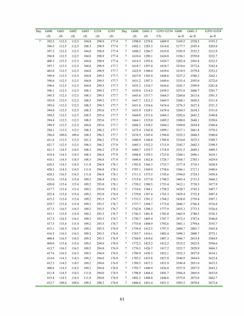
61
Day G600 G601 G602 G603 G354 G393 Day G600 G601-3 G393+G354 G600 G601-3 G393+G354 cfs cfs cfs cfs cfs cfs cfs cfs Cfs ac-ft ac-ft ac-ft
7 392.5 112.5 112.5 104.8 298.9 177.4 7 1598.0 1279.8 1609.9 3169.5 2538.5 3193.2 396.5 112.5 112.5 108.3 298.9 177.4 7 1602.1 1283.3 1614.8 3177.7 2545.4 3203.0 397.2 112.5 112.5 104.8 298.9 177.4 7 1606.2 1286.7 1619.8 3185.9 2552.2 3212.9 396.8 112.5 112.5 104.8 298.9 177.4 7 1610.4 1290.1 1624.8 3194.1 2559.0 3222.7 400.3 112.5 112.5 104.8 298.9 177.4 7 1614.5 1293.6 1629.7 3202.4 2565.8 3232.5 397.1 112.5 112.5 104.8 298.9 177.7 7 1618.7 1297.0 1634.7 3210.6 2572.6 3242.4 402.0 112.5 112.5 104.8 298.9 177.7 7 1622.9 1300.4 1639.6 3218.9 2579.4 3252.2 399.4 112.5 112.5 104.8 299.5 177.7 7 1627.0 1303.9 1644.6 3227.2 2586.2 3262.1 398.6 112.5 112.5 104.8 299.5 177.7 7 1631.2 1307.3 1649.6 3235.4 2593.0 3272.0 398.6 112.5 112.5 104.8 299.5 177.7 7 1635.3 1310.7 1654.6 3243.7 2599.9 3281.8 396.1 112.5 112.5 108.3 299.5 177.7 7 1639.4 1314.2 1659.5 3251.8 2606.7 3291.7 395.5 112.5 112.5 108.3 299.5 177.7 7 1643.6 1317.7 1664.5 3260.0 2613.6 3301.5 393.0 112.5 112.5 108.3 299.5 177.7 7 1647.7 1321.2 1669.5 3268.1 2620.5 3311.4 395.6 112.5 112.5 108.3 299.5 177.7 7 1651.8 1324.6 1674.4 3276.3 2627.4 3321.3 394.8 112.5 112.5 108.3 295.6 177.7 7 1655.9 1328.1 1679.4 3284.5 2634.3 3331.0 394.5 112.5 112.5 108.3 295.6 177.7 7 1660.0 1331.6 1684.3 3292.6 2641.2 3340.8 394.4 112.5 112.5 108.3 295.6 177.7 7 1664.1 1335.0 1689.2 3300.8 2648.1 3350.6 398.9 112.5 112.5 104.8 295.6 177.7 7 1668.3 1338.5 1694.2 3309.0 2654.9 3360.4 394.1 112.5 112.5 108.3 296.2 177.7 7 1672.4 1342.0 1699.1 3317.1 2661.8 3370.2 396.0 109.6 109.6 108.3 296.2 177.7 7 1676.5 1345.4 1704.0 3325.3 2668.5 3380.0 421.6 112.5 112.5 101.2 296.2 177.9 7 1680.9 1348.8 1709.0 3334.0 2675.3 3389.7 421.7 112.5 112.5 108.3 296.2 177.9 7 1685.3 1352.2 1713.9 3342.7 2682.2 3399.5 421.3 114.5 114.5 108.3 296.2 177.9 7 1689.7 1355.7 1718.9 3351.5 2689.1 3409.3 418.4 114.5 114.5 108.3 296.8 177.9 7 1694.0 1359.3 1723.8 3360.1 2696.1 3419.1 418.1 114.5 114.5 108.3 296.8 177.9 7 1698.4 1362.8 1728.7 3368.7 2703.1 3429.0 420.5 114.5 114.5 111.8 296.8 178.1 7 1702.8 1366.3 1733.7 3377.4 2710.1 3438.8 420.3 114.5 114.5 111.8 296.8 178.1 7 1707.1 1369.9 1738.6 3386.1 2717.1 3448.6 420.2 116.5 116.5 111.8 296.8 178.1 7 1711.5 1373.5 1743.6 3394.8 2724.3 3458.4 415.6 115.4 115.4 109.2 296.8 178.1 7 1715.8 1377.0 1748.5 3403.4 2731.3 3468.2 420.0 115.4 115.4 109.2 293.0 178.1 7 1720.2 1380.5 1753.4 3412.1 2738.3 3477.9 417.7 115.4 115.4 109.2 293.0 178.1 7 1724.6 1384.1 1758.3 3420.7 2745.3 3487.7 422.4 115.4 115.4 109.2 293.0 178.4 7 1729.0 1387.6 1763.3 3429.4 2752.4 3497.4 415.2 115.4 115.4 109.2 293.5 176.7 7 1733.3 1391.2 1768.2 3438.0 2759.4 3507.1 419.7 115.4 115.4 109.2 293.5 176.7 7 1737.7 1394.7 1773.0 3446.7 2766.4 3516.8 417.5 116.5 116.5 109.2 293.5 176.7 7 1742.0 1398.3 1777.9 3455.3 2773.5 3526.6 415.1 115.4 115.4 109.2 293.5 176.7 7 1746.3 1401.8 1782.8 3463.9 2780.5 3536.3 417.5 116.5 116.5 109.2 293.5 176.7 7 1750.7 1405.4 1787.7 3472.5 2787.6 3546.0 417.5 115.4 115.4 109.2 293.5 176.7 7 1755.0 1408.9 1792.6 3481.1 2794.6 3555.7 415.1 116.5 116.5 109.2 293.5 176.9 7 1759.4 1412.5 1797.5 3489.7 2801.7 3565.4 416.5 116.5 116.5 109.2 293.5 176.9 7 1763.7 1416.1 1802.4 3498.3 2808.7 3575.1 408.8 116.5 116.5 109.2 293.5 176.9 7 1768.0 1419.6 1807.3 3506.7 2815.8 3584.9 408.0 115.4 115.4 109.2 294.0 176.9 7 1772.2 1423.2 1812.2 3515.2 2822.8 3594.6 413.7 116.5 116.5 109.2 294.0 176.9 7 1776.5 1426.7 1817.2 3523.7 2829.9 3604.3 417.6 116.5 116.5 109.2 294.0 176.9 7 1780.9 1430.3 1822.1 3532.3 2837.0 3614.1 414.0 114.5 114.5 109.2 294.0 176.9 7 1785.2 1433.8 1827.0 3540.9 2844.0 3623.8 412.3 114.5 114.5 109.2 294.0 176.9 7 1789.5 1437.3 1831.9 3549.4 2851.0 3633.5 408.6 114.5 114.5 109.2 294.0 176.9 7 1793.7 1440.9 1836.8 3557.9 2857.9 3643.2 411.8 114.5 114.5 111.8 294.0 176.9 7 1798.0 1444.4 1841.7 3566.4 2865.0 3653.0 415.4 114.5 114.5 111.8 294.0 176.9 7 1802.3 1448.0 1846.6 3575.0 2872.0 3662.7 412.7 109.6 109.6 109.2 290.2 176.9 7 1806.6 1451.4 1851.5 3583.5 2878.8 3672.4

62
Day G600 G601 G602 G603 G354 G393 Day G600 G601-3 G393+G354 G600 G601-3 G393+G354 cfs cfs cfs cfs cfs cfs cfs cfs Cfs ac-ft ac-ft ac-ft
394.9 108.7 108.7 104.8 290.2 176.9 7 1810.8 1454.7 1856.3 3591.6 2885.5 3682.0 387.7 103.1 103.1 93.0 290.2 176.9 7 1814.8 1457.9 1861.2 3599.7 2891.7 3691.7 391.0 102.3 102.3 92.2 289.7 176.9 7 1818.9 1460.9 1866.0 3607.7 2897.8 3701.3 390.2 102.3 102.3 91.4 289.7 176.9 7 1822.9 1464.0 1870.9 3615.8 2903.9 3710.9 385.9 99.5 99.5 86.9 289.7 176.9 7 1827.0 1467.0 1875.8 3623.8 2909.8 3720.6 395.1 99.5 99.5 86.9 289.7 176.9 7 1831.1 1470.0 1880.6 3631.9 2915.7 3730.2 393.5 97.6 97.6 86.1 289.7 176.9 7 1835.2 1472.9 1885.5 3640.1 2921.5 3739.9 392.9 98.7 98.7 82.3 289.7 176.9 7 1839.3 1475.8 1890.4 3648.2 2927.3 3749.5 395.2 96.8 96.8 81.6 289.7 176.9 7 1843.4 1478.7 1895.2 3656.3 2933.0 3759.2 394.4 97.9 97.9 81.6 289.7 175.3 7 1847.5 1481.6 1900.1 3664.5 2938.7 3768.8 389.6 97.9 97.9 77.7 289.7 175.3 7 1851.5 1484.4 1904.9 3672.5 2944.4 3778.4 389.5 96.0 96.0 80.8 289.7 175.3 7 1855.6 1487.3 1909.7 3680.6 2950.0 3788.0 395.3 96.0 96.0 80.8 289.7 175.3 7 1859.7 1490.1 1914.6 3688.8 2955.6 3797.6 395.9 97.1 97.1 77.0 285.9 173.7 7 1863.8 1492.9 1919.4 3696.9 2961.3 3807.1 391.5 95.2 95.2 80.1 285.9 173.7 7 1867.9 1495.8 1924.2 3705.0 2966.8 3816.6 393.6 95.2 95.2 80.1 286.4 173.7 7 1872.0 1498.6 1929.0 3713.2 2972.4 3826.1 395.5 95.2 95.2 80.1 286.4 173.7 7 1876.1 1501.4 1933.7 3721.3 2978.0 3835.6 389.5 96.3 96.3 76.3 286.4 172.1 7 1880.2 1504.2 1938.5 3729.4 2983.6 3845.1 389.6 96.3 96.3 79.4 286.4 172.1 7 1884.3 1507.0 1943.3 3737.4 2989.2 3854.5 391.5 96.3 96.3 79.4 286.4 172.1 7 1888.3 1509.9 1948.1 3745.5 2994.8 3864.0 391.2 94.4 94.4 79.4 282.6 172.1 7 1892.4 1512.7 1952.8 3753.6 3000.3 3873.4 391.3 95.5 95.5 79.4 282.6 170.4 7 1896.5 1515.5 1957.5 3761.7 3005.9 3882.8 395.5 94.4 94.4 82.3 282.6 170.4 7 1900.6 1518.3 1962.2 3769.9 3011.5 3892.1 389.2 95.5 95.5 78.6 282.6 170.6 7 1904.7 1521.1 1967.0 3777.9 3017.1 3901.5 393.6 95.5 95.5 78.6 282.6 169.0 7 1908.8 1523.9 1971.7 3786.0 3022.7 3910.8 399.3 95.5 95.5 78.6 283.1 169.0 7 1912.9 1526.7 1976.4 3794.3 3028.2 3920.2 391.7 95.5 95.5 81.5 283.1 169.0 7 1917.0 1529.6 1981.1 3802.4 3033.9 3929.5 395.3 95.5 95.5 81.5 279.4 169.0 7 1921.1 1532.4 1985.8 3810.5 3039.5 3938.8 393.2 94.7 94.7 81.5 279.4 167.4 7 1925.2 1535.2 1990.4 3818.7 3045.1 3948.0 402.9 94.7 94.7 81.5 279.4 167.4 7 1929.4 1538.0 1995.1 3827.0 3050.7 3957.2 399.1 94.7 94.7 84.3 279.9 167.6 7 1933.6 1540.9 1999.7 3835.2 3056.4 3966.5 398.8 94.7 94.7 84.3 279.9 167.6 7 1937.7 1543.7 2004.4 3843.5 3062.0 3975.7 387.2 94.7 94.7 80.8 276.1 166.0 7 1941.8 1546.6 2009.0 3851.5 3067.6 3984.9 395.3 94.7 94.7 80.8 276.1 166.0 7 1945.9 1549.4 2013.6 3859.6 3073.2 3994.0 389.2 94.7 94.7 80.8 276.1 166.0 7 1949.9 1552.2 2018.2 3867.7 3078.7 4003.1 389.5 94.7 94.7 83.5 276.1 164.6 7 1954.0 1555.0 2022.8 3875.7 3084.4 4012.2 389.5 94.7 94.7 83.5 276.6 164.6 7 1958.0 1557.9 2027.4 3883.8 3090.0 4021.4 397.1 95.7 95.7 83.5 276.6 164.6 7 1962.2 1560.7 2032.0 3892.0 3095.7 4030.5 391.5 93.9 93.9 83.5 272.8 164.6 7 1966.3 1563.6 2036.6 3900.1 3101.3 4039.5 401.4 93.9 93.9 83.5 272.8 163.0 7 1970.4 1566.4 2041.1 3908.4 3106.9 4048.5 393.3 93.9 93.9 86.0 272.8 163.0 7 1974.5 1569.2 2045.6 3916.5 3112.6 4057.5 397.1 93.9 93.9 86.0 273.3 163.2 7 1978.7 1572.1 2050.2 3924.7 3118.2 4066.5 397.7 93.9 93.9 86.0 273.3 163.2 7 1982.8 1574.9 2054.7 3932.9 3123.9 4075.6 395.0 93.9 93.9 82.7 269.6 163.2 7 1986.9 1577.8 2059.2 3941.1 3129.5 4084.5 404.6 93.9 93.9 82.7 269.6 161.6 7 1991.1 1580.6 2063.7 3949.4 3135.1 4093.4 396.6 93.9 93.9 82.7 269.6 161.6 7 1995.3 1583.4 2068.2 3957.6 3140.6 4102.3
8 398.8 93.9 93.9 85.3 269.6 161.6 8 1999.4 1586.2 2072.7 3965.9 3146.3 4111.2 397.1 94.9 94.9 85.3 269.6 161.6 8 2003.6 1589.1 2077.2 3974.1 3152.0 4120.1 400.5 93.9 93.9 85.3 270.0 160.2 8 2007.7 1591.9 2081.7 3982.4 3157.6 4129.0 396.6 94.9 94.9 85.3 266.3 160.2 8 2011.9 1594.8 2086.1 3990.5 3163.3 4137.8
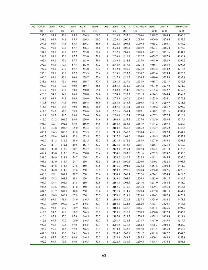
63
Day G600 G601 G602 G603 G354 G393 Day G600 G601-3 G393+G354 G600 G601-3 G393+G354 cfs cfs cfs cfs cfs cfs cfs cfs Cfs ac-ft ac-ft ac-ft
395.0 93.9 93.9 85.3 266.3 160.2 8 2016.0 1597.6 2090.6 3998.7 3168.9 4146.6 398.6 94.9 94.9 85.3 266.3 160.2 8 2020.1 1600.5 2095.0 4006.9 3174.6 4155.5 399.1 94.9 94.9 85.3 266.3 158.6 8 2024.3 1603.4 2099.4 4015.2 3180.3 4164.2 392.7 93.1 93.1 87.7 266.3 158.6 8 2028.4 1606.2 2103.9 4023.3 3186.0 4173.0 394.7 93.1 93.1 87.7 263.0 158.6 8 2032.5 1609.1 2108.3 4031.5 3191.6 4181.7 398.3 93.1 93.1 87.7 263.0 158.8 8 2036.6 1611.9 2112.7 4039.7 3197.3 4190.4 402.4 93.1 93.1 87.7 263.0 158.8 8 2040.8 1614.8 2117.0 4048.0 3202.9 4199.2 392.7 93.1 93.1 87.7 263.0 157.2 8 2044.9 1617.6 2121.4 4056.1 3208.6 4207.8 392.2 93.1 93.1 87.7 263.0 157.2 8 2049.0 1620.5 2125.8 4064.2 3214.2 4216.5 395.0 93.1 93.1 87.7 263.3 157.4 8 2053.1 1623.3 2130.2 4072.4 3219.9 4225.2 400.0 93.1 93.1 90.0 259.7 157.4 8 2057.3 1626.2 2134.5 4080.6 3225.6 4233.8 388.6 93.1 93.1 90.0 259.7 157.4 8 2061.3 1629.1 2138.9 4088.7 3231.3 4242.5 400.7 93.1 93.1 90.0 259.7 155.8 8 2065.5 1632.0 2143.2 4097.0 3237.0 4251.0 419.2 93.1 93.1 90.0 260.0 155.8 8 2069.9 1634.8 2147.5 4105.6 3242.7 4259.6 420.6 94.1 94.1 86.0 260.0 156.0 8 2074.3 1637.7 2151.9 4114.3 3248.4 4268.2 418.1 94.9 94.9 86.9 260.0 156.0 8 2078.6 1640.6 2156.2 4122.9 3254.1 4276.8 417.8 94.9 94.9 90.0 256.4 156.0 8 2083.0 1643.5 2160.5 4131.6 3259.9 4285.3 415.6 94.9 94.9 90.0 256.6 156.0 8 2087.3 1646.4 2164.8 4140.2 3265.7 4293.9 411.3 96.7 96.7 93.0 256.6 154.6 8 2091.6 1649.4 2169.1 4148.7 3271.6 4302.4 419.1 96.7 96.7 93.0 256.6 154.6 8 2096.0 1652.4 2173.4 4157.3 3277.5 4310.9 415.0 101.2 101.2 93.0 256.6 154.6 8 2100.3 1655.5 2177.6 4165.9 3283.6 4319.4 401.7 102.1 102.1 93.0 256.9 154.6 8 2104.5 1658.6 2181.9 4174.2 3289.8 4327.9 411.3 103.8 103.8 105.0 253.3 154.7 8 2108.7 1661.8 2186.2 4182.7 3296.2 4336.3 406.1 106.5 106.5 111.8 253.3 153.2 8 2113.0 1665.2 2190.4 4191.1 3302.9 4344.7 406.2 108.4 108.4 112.8 253.5 153.2 8 2117.2 1668.6 2194.6 4199.5 3309.7 4353.1 406.0 111.2 111.2 118.6 253.5 153.3 8 2121.4 1672.2 2198.9 4207.9 3316.8 4361.5 399.0 111.1 111.1 119.6 253.7 153.3 8 2125.6 1675.7 2203.1 4216.1 3323.8 4369.9 404.6 113.0 113.0 120.7 253.7 153.4 8 2129.8 1679.4 2207.4 4224.5 3331.0 4378.3 408.4 113.0 113.0 123.6 250.0 153.4 8 2134.1 1683.0 2211.6 4232.9 3338.2 4386.6 398.0 114.9 114.9 124.7 250.1 153.4 8 2138.2 1686.7 2215.8 4241.1 3345.5 4395.0 403.6 113.9 113.9 124.7 250.1 153.5 8 2142.4 1690.4 2220.0 4249.5 3352.8 4403.3 401.2 114.8 114.8 127.6 250.1 153.5 8 2146.6 1694.1 2224.2 4257.8 3360.2 4411.7 399.4 114.8 114.8 127.6 250.1 153.5 8 2150.7 1697.8 2228.4 4266.0 3367.6 4420.0 400.6 109.1 109.1 128.7 250.1 153.6 8 2154.9 1701.4 2232.6 4274.3 3374.8 4428.3 403.8 108.3 108.3 118.8 250.1 153.6 8 2159.1 1704.9 2236.8 4282.6 3381.7 4436.7 404.9 104.4 104.4 117.8 250.1 153.6 8 2163.3 1708.3 2241.0 4291.0 3388.4 4445.0 408.5 103.6 103.6 111.8 250.1 153.6 8 2167.6 1711.6 2245.2 4299.4 3395.0 4453.4 404.6 101.7 101.7 110.8 250.1 153.6 8 2171.8 1714.9 2249.4 4307.8 3401.5 4461.7 407.1 100.9 100.9 107.9 250.1 153.7 8 2176.1 1718.1 2253.6 4316.2 3407.9 4470.1 407.9 99.0 99.0 104.9 246.5 153.7 8 2180.3 1721.3 2257.8 4324.6 3414.2 4478.3 407.7 100.0 100.0 103.9 246.5 153.7 8 2184.6 1724.5 2262.0 4333.1 3420.5 4486.6 409.9 99.2 99.2 100.9 246.5 153.7 8 2188.8 1727.6 2266.1 4341.5 3426.6 4494.9 412.2 99.2 99.2 100.9 246.5 155.2 8 2193.1 1730.7 2270.3 4350.0 3432.8 4503.2 410.6 97.3 97.3 97.9 246.5 153.7 8 2197.4 1733.7 2274.5 4358.5 3438.9 4511.4 412.1 97.3 97.3 100.0 246.5 153.7 8 2201.7 1736.8 2278.7 4367.0 3445.0 4519.7 400.6 93.9 93.9 97.0 246.5 153.7 8 2205.9 1739.8 2282.8 4375.3 3450.8 4528.0 395.7 96.5 96.5 97.0 246.5 153.7 8 2210.0 1742.8 2287.0 4383.5 3456.8 4536.2 401.0 93.9 93.9 96.1 246.5 153.7 8 2214.2 1745.8 2291.2 4391.8 3462.7 4544.5 400.8 95.7 95.7 93.0 246.5 153.7 8 2218.3 1748.7 2295.3 4400.1 3468.6 4552.8 402.2 93.9 93.9 93.0 246.5 153.8 8 2222.5 1751.6 2299.5 4408.4 3474.4 4561.1

64
Day G600 G601 G602 G603 G354 G393 Day G600 G601-3 G393+G354 G600 G601-3 G393+G354 cfs cfs cfs cfs cfs cfs cfs cfs Cfs ac-ft ac-ft ac-ft
401.9 94.9 94.9 93.0 246.5 153.7 8 2226.7 1754.6 2303.7 4416.7 3480.2 4569.3 403.7 94.9 94.9 92.2 246.5 153.8 8 2230.9 1757.5 2307.8 4425.0 3486.0 4577.6 401.1 94.9 94.9 92.2 246.5 153.8 8 2235.1 1760.5 2312.0 4433.3 3491.9 4585.9 402.4 93.1 93.1 92.2 246.5 153.8 8 2239.3 1763.4 2316.2 4441.6 3497.6 4594.1 401.8 93.1 93.1 92.2 246.5 153.8 8 2243.5 1766.3 2320.3 4449.9 3503.4 4602.4 402.1 93.1 93.1 92.2 246.5 152.2 8 2247.7 1769.2 2324.5 4458.2 3509.1 4610.6 402.3 93.1 93.1 92.2 243.0 152.2 8 2251.9 1772.1 2328.6 4466.5 3514.9 4618.8 404.8 94.1 94.1 92.2 243.0 152.2 8 2256.1 1775.0 2332.7 4474.9 3520.7 4627.0 402.7 93.1 93.1 91.3 243.0 152.2 8 2260.3 1777.9 2336.8 4483.2 3526.4 4635.1 405.0 94.1 94.1 91.3 243.0 152.2 8 2264.5 1780.8 2341.0 4491.6 3532.2 4643.3 403.2 94.1 94.1 91.3 243.0 152.2 8 2268.7 1783.7 2345.1 4499.9 3538.0 4651.5 405.3 94.1 94.1 91.3 243.0 150.6 8 2272.9 1786.6 2349.2 4508.3 3543.7 4659.6 403.3 94.1 94.1 91.3 243.0 150.6 8 2277.1 1789.5 2353.3 4516.6 3549.5 4667.7 403.5 92.3 92.3 91.3 243.0 150.6 8 2281.3 1792.4 2357.4 4525.0 3555.2 4675.9 403.2 92.3 92.3 91.3 243.0 150.6 8 2285.5 1795.3 2361.5 4533.3 3560.9 4684.0 401.4 92.3 92.3 93.4 239.4 150.6 8 2289.7 1798.2 2365.5 4541.6 3566.6 4692.1 403.7 92.3 92.3 93.4 239.4 150.6 8 2293.9 1801.1 2369.6 4549.9 3572.4 4700.1 406.2 92.3 92.3 93.4 239.4 150.6 8 2298.1 1804.0 2373.7 4558.3 3578.1 4708.2 401.9 92.3 92.3 93.4 239.4 149.1 8 2302.3 1806.8 2377.7 4566.6 3583.9 4716.2 401.7 92.3 92.3 93.4 239.4 149.1 8 2306.5 1809.7 2381.8 4574.9 3589.6 4724.2 404.3 92.3 92.3 93.4 239.4 149.1 8 2310.7 1812.6 2385.8 4583.3 3595.4 4732.3 401.8 93.3 93.3 93.4 239.4 149.1 8 2314.9 1815.6 2389.9 4591.6 3601.2 4740.3 404.2 92.3 92.3 93.4 239.4 149.1 8 2319.1 1818.5 2393.9 4599.9 3606.9 4748.3 406.8 93.3 93.3 93.4 235.9 149.1 8 2323.3 1821.4 2397.9 4608.3 3612.7 4756.3 406.0 93.3 93.3 95.5 235.9 147.6 8 2327.6 1824.3 2401.9 4616.7 3618.5 4764.2 405.4 93.3 93.3 95.5 235.9 147.6 8 2331.8 1827.2 2405.9 4625.1 3624.3 4772.1 400.0 93.3 93.3 92.6 235.9 147.6 8 2336.0 1830.2 2409.9 4633.4 3630.1 4780.0 404.1 93.3 93.3 92.6 235.9 147.6 8 2340.2 1833.1 2413.9 4641.7 3635.9 4788.0 403.5 93.3 93.3 92.6 235.9 147.6 8 2344.4 1836.0 2417.9 4650.1 3641.6 4795.9 400.4 93.3 93.3 92.6 235.9 147.6 8 2348.5 1838.9 2421.9 4658.3 3647.4 4803.8 402.2 93.3 93.3 92.6 232.3 146.1 8 2352.7 1841.8 2425.8 4666.6 3653.2 4811.6 399.9 93.3 93.3 92.6 232.3 146.1 8 2356.9 1844.7 2429.8 4674.9 3658.9 4819.4 399.9 93.3 93.3 92.6 232.3 146.1 8 2361.1 1847.6 2433.7 4683.2 3664.7 4827.3 402.3 91.5 91.5 92.6 232.3 146.1 8 2365.3 1850.5 2437.6 4691.5 3670.4 4835.1 402.2 93.3 93.3 92.6 232.3 146.1 8 2369.4 1853.4 2441.6 4699.8 3676.2 4842.9 399.8 91.5 91.5 94.6 232.3 146.1 8 2373.6 1856.3 2445.5 4708.1 3681.9 4850.7 399.7 91.5 91.5 94.6 232.3 146.1 8 2377.8 1859.2 2449.5 4716.3 3687.6 4858.5 397.7 91.5 91.5 94.6 228.8 146.1 8 2381.9 1862.0 2453.4 4724.5 3693.4 4866.3 399.8 91.5 91.5 94.6 228.8 144.5 8 2386.1 1864.9 2457.3 4732.8 3699.1 4874.0 395.4 91.5 91.5 94.6 228.8 144.5 8 2390.2 1867.8 2461.2 4741.0 3704.8 4881.7 397.4 91.5 91.5 94.6 228.8 144.5 8 2394.3 1870.7 2465.0 4749.2 3710.6 4889.4 390.7 91.5 91.5 94.6 228.8 144.5 8 2398.4 1873.6 2468.9 4757.2 3716.3 4897.1
9 394.4 91.5 91.5 94.6 225.3 144.5 9 2402.5 1876.5 2472.8 4765.4 3722.0 4904.8 395.6 91.5 91.5 94.6 225.3 143.0 9 2406.6 1879.4 2476.6 4773.6 3727.8 4912.4 396.6 92.5 92.5 94.6 225.3 143.0 9 2410.8 1882.3 2480.5 4781.8 3733.6 4920.0 397.8 91.5 91.5 94.6 225.3 143.0 9 2414.9 1885.2 2484.3 4790.0 3739.3 4927.6 396.3 92.5 92.5 94.6 225.3 143.0 9 2419.0 1888.1 2488.1 4798.2 3745.1 4935.2 399.6 92.5 92.5 94.6 225.3 143.0 9 2423.2 1891.0 2492.0 4806.4 3750.8 4942.8 395.8 91.5 91.5 94.6 225.3 143.0 9 2427.3 1893.9 2495.8 4814.6 3756.6 4950.4 396.2 91.5 91.5 96.5 225.3 143.0 9 2431.5 1896.8 2499.6 4822.8 3762.4 4958.0
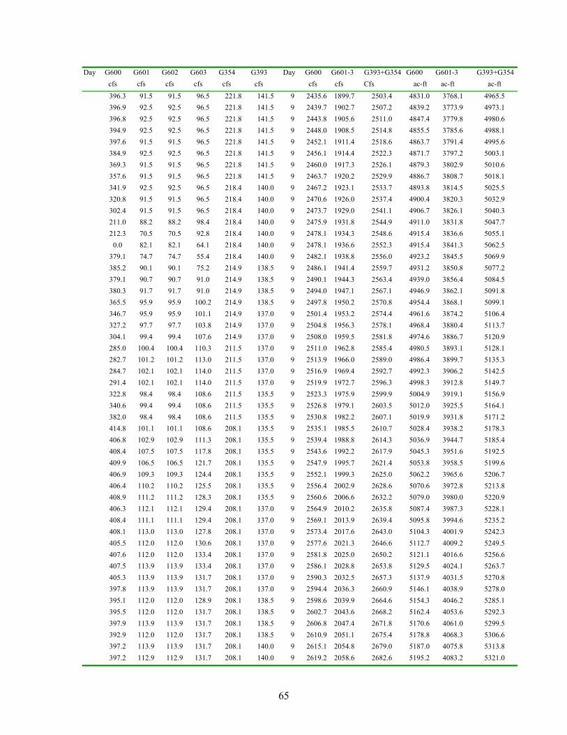
65
Day G600 G601 G602 G603 G354 G393 Day G600 G601-3 G393+G354 G600 G601-3 G393+G354 cfs cfs cfs cfs cfs cfs cfs cfs Cfs ac-ft ac-ft ac-ft
396.3 91.5 91.5 96.5 221.8 141.5 9 2435.6 1899.7 2503.4 4831.0 3768.1 4965.5 396.9 92.5 92.5 96.5 221.8 141.5 9 2439.7 1902.7 2507.2 4839.2 3773.9 4973.1 396.8 92.5 92.5 96.5 221.8 141.5 9 2443.8 1905.6 2511.0 4847.4 3779.8 4980.6 394.9 92.5 92.5 96.5 221.8 141.5 9 2448.0 1908.5 2514.8 4855.5 3785.6 4988.1 397.6 91.5 91.5 96.5 221.8 141.5 9 2452.1 1911.4 2518.6 4863.7 3791.4 4995.6 384.9 92.5 92.5 96.5 221.8 141.5 9 2456.1 1914.4 2522.3 4871.7 3797.2 5003.1 369.3 91.5 91.5 96.5 221.8 141.5 9 2460.0 1917.3 2526.1 4879.3 3802.9 5010.6 357.6 91.5 91.5 96.5 221.8 141.5 9 2463.7 1920.2 2529.9 4886.7 3808.7 5018.1 341.9 92.5 92.5 96.5 218.4 140.0 9 2467.2 1923.1 2533.7 4893.8 3814.5 5025.5 320.8 91.5 91.5 96.5 218.4 140.0 9 2470.6 1926.0 2537.4 4900.4 3820.3 5032.9 302.4 91.5 91.5 96.5 218.4 140.0 9 2473.7 1929.0 2541.1 4906.7 3826.1 5040.3 211.0 88.2 88.2 98.4 218.4 140.0 9 2475.9 1931.8 2544.9 4911.0 3831.8 5047.7 212.3 70.5 70.5 92.8 218.4 140.0 9 2478.1 1934.3 2548.6 4915.4 3836.6 5055.1 0.0 82.1 82.1 64.1 218.4 140.0 9 2478.1 1936.6 2552.3 4915.4 3841.3 5062.5 379.1 74.7 74.7 55.4 218.4 140.0 9 2482.1 1938.8 2556.0 4923.2 3845.5 5069.9 385.2 90.1 90.1 75.2 214.9 138.5 9 2486.1 1941.4 2559.7 4931.2 3850.8 5077.2 379.1 90.7 90.7 91.0 214.9 138.5 9 2490.1 1944.3 2563.4 4939.0 3856.4 5084.5 380.3 91.7 91.7 91.0 214.9 138.5 9 2494.0 1947.1 2567.1 4946.9 3862.1 5091.8 365.5 95.9 95.9 100.2 214.9 138.5 9 2497.8 1950.2 2570.8 4954.4 3868.1 5099.1 346.7 95.9 95.9 101.1 214.9 137.0 9 2501.4 1953.2 2574.4 4961.6 3874.2 5106.4 327.2 97.7 97.7 103.8 214.9 137.0 9 2504.8 1956.3 2578.1 4968.4 3880.4 5113.7 304.1 99.4 99.4 107.6 214.9 137.0 9 2508.0 1959.5 2581.8 4974.6 3886.7 5120.9 285.0 100.4 100.4 110.3 211.5 137.0 9 2511.0 1962.8 2585.4 4980.5 3893.1 5128.1 282.7 101.2 101.2 113.0 211.5 137.0 9 2513.9 1966.0 2589.0 4986.4 3899.7 5135.3 284.7 102.1 102.1 114.0 211.5 137.0 9 2516.9 1969.4 2592.7 4992.3 3906.2 5142.5 291.4 102.1 102.1 114.0 211.5 137.0 9 2519.9 1972.7 2596.3 4998.3 3912.8 5149.7 322.8 98.4 98.4 108.6 211.5 135.5 9 2523.3 1975.9 2599.9 5004.9 3919.1 5156.9 340.6 99.4 99.4 108.6 211.5 135.5 9 2526.8 1979.1 2603.5 5012.0 3925.5 5164.1 382.0 98.4 98.4 108.6 211.5 135.5 9 2530.8 1982.2 2607.1 5019.9 3931.8 5171.2 414.8 101.1 101.1 108.6 208.1 135.5 9 2535.1 1985.5 2610.7 5028.4 3938.2 5178.3 406.8 102.9 102.9 111.3 208.1 135.5 9 2539.4 1988.8 2614.3 5036.9 3944.7 5185.4 408.4 107.5 107.5 117.8 208.1 135.5 9 2543.6 1992.2 2617.9 5045.3 3951.6 5192.5 409.9 106.5 106.5 121.7 208.1 135.5 9 2547.9 1995.7 2621.4 5053.8 3958.5 5199.6 406.9 109.3 109.3 124.4 208.1 135.5 9 2552.1 1999.3 2625.0 5062.2 3965.6 5206.7 406.4 110.2 110.2 125.5 208.1 135.5 9 2556.4 2002.9 2628.6 5070.6 3972.8 5213.8 408.9 111.2 111.2 128.3 208.1 135.5 9 2560.6 2006.6 2632.2 5079.0 3980.0 5220.9 406.3 112.1 112.1 129.4 208.1 137.0 9 2564.9 2010.2 2635.8 5087.4 3987.3 5228.1 408.4 111.1 111.1 129.4 208.1 137.0 9 2569.1 2013.9 2639.4 5095.8 3994.6 5235.2 408.1 113.0 113.0 127.8 208.1 137.0 9 2573.4 2017.6 2643.0 5104.3 4001.9 5242.3 405.5 112.0 112.0 130.6 208.1 137.0 9 2577.6 2021.3 2646.6 5112.7 4009.2 5249.5 407.6 112.0 112.0 133.4 208.1 137.0 9 2581.8 2025.0 2650.2 5121.1 4016.6 5256.6 407.5 113.9 113.9 133.4 208.1 137.0 9 2586.1 2028.8 2653.8 5129.5 4024.1 5263.7 405.3 113.9 113.9 131.7 208.1 137.0 9 2590.3 2032.5 2657.3 5137.9 4031.5 5270.8 397.8 113.9 113.9 131.7 208.1 137.0 9 2594.4 2036.3 2660.9 5146.1 4038.9 5278.0 395.1 112.0 112.0 128.9 208.1 138.5 9 2598.6 2039.9 2664.6 5154.3 4046.2 5285.1 395.5 112.0 112.0 131.7 208.1 138.5 9 2602.7 2043.6 2668.2 5162.4 4053.6 5292.3 397.9 113.9 113.9 131.7 208.1 138.5 9 2606.8 2047.4 2671.8 5170.6 4061.0 5299.5 392.9 112.0 112.0 131.7 208.1 138.5 9 2610.9 2051.1 2675.4 5178.8 4068.3 5306.6 397.2 113.9 113.9 131.7 208.1 140.0 9 2615.1 2054.8 2679.0 5187.0 4075.8 5313.8 397.2 112.9 112.9 131.7 208.1 140.0 9 2619.2 2058.6 2682.6 5195.2 4083.2 5321.0

66
Day G600 G601 G602 G603 G354 G393 Day G600 G601-3 G393+G354 G600 G601-3 G393+G354 cfs cfs cfs cfs cfs cfs cfs cfs Cfs ac-ft ac-ft ac-ft
397.0 112.9 112.9 130.0 208.1 140.0 9 2623.3 2062.3 2686.3 5203.4 4090.5 5328.2 394.2 113.9 113.9 130.0 208.1 140.0 9 2627.4 2066.0 2689.9 5211.5 4097.9 5335.4 396.8 112.9 112.9 130.0 208.1 140.0 9 2631.6 2069.7 2693.5 5219.7 4105.3 5342.6 396.8 112.9 112.9 130.0 208.1 141.5 9 2635.7 2073.4 2697.2 5227.9 4112.6 5349.8 393.9 112.9 112.9 130.0 208.1 141.5 9 2639.8 2077.1 2700.8 5236.1 4120.0 5357.0 394.2 112.9 112.9 130.0 211.5 141.5 9 2643.9 2080.8 2704.5 5244.2 4127.3 5364.3 396.1 112.9 112.9 128.3 211.5 141.5 9 2648.0 2084.5 2708.1 5252.4 4134.6 5371.6 393.6 112.9 112.9 131.2 211.5 143.0 9 2652.1 2088.2 2711.8 5260.5 4142.0 5378.9 391.4 112.9 112.9 128.3 211.5 143.0 9 2656.2 2091.9 2715.5 5268.6 4149.3 5386.3 396.0 112.9 112.9 128.3 211.5 143.0 9 2660.3 2095.6 2719.2 5276.8 4156.6 5393.6 393.4 112.9 112.9 128.3 211.5 143.0 9 2664.4 2099.3 2722.9 5284.9 4163.9 5400.9 396.0 112.9 112.9 128.3 211.5 143.0 9 2668.6 2103.0 2726.6 5293.1 4171.3 5408.2 395.8 112.9 112.9 131.2 211.5 144.5 9 2672.7 2106.7 2730.3 5301.3 4178.6 5415.6 393.2 112.9 112.9 126.5 211.5 144.5 9 2676.8 2110.4 2734.0 5309.4 4185.9 5422.9 395.8 112.9 112.9 126.5 211.5 144.5 9 2680.9 2114.0 2737.7 5317.6 4193.2 5430.3 395.7 112.9 112.9 126.5 211.5 144.5 9 2685.0 2117.7 2741.4 5325.8 4200.5 5437.7 395.6 111.8 111.8 129.4 214.9 144.5 9 2689.1 2121.4 2745.2 5333.9 4207.8 5445.1 395.4 111.8 111.8 129.4 214.9 146.1 9 2693.3 2125.1 2749.0 5342.1 4215.1 5452.5 395.0 111.8 111.8 129.4 214.9 146.1 9 2697.4 2128.7 2752.7 5350.3 4222.3 5460.0 390.4 111.8 111.8 129.4 214.9 146.1 9 2701.4 2132.4 2756.5 5358.3 4229.6 5467.5 392.8 111.8 111.8 129.4 214.9 146.1 9 2705.5 2136.1 2760.2 5366.4 4236.9 5474.9 390.2 111.8 111.8 127.6 214.9 146.1 9 2709.6 2139.8 2764.0 5374.5 4244.2 5482.4 392.5 111.8 111.8 127.6 214.9 146.1 9 2713.7 2143.4 2767.8 5382.6 4251.5 5489.8 392.4 111.8 111.8 127.6 214.9 147.6 9 2717.8 2147.1 2771.5 5390.7 4258.7 5497.3 392.1 111.8 111.8 127.6 214.9 147.6 9 2721.9 2150.7 2775.3 5398.8 4266.0 5504.8 390.1 111.8 111.8 127.6 214.9 147.6 9 2725.9 2154.4 2779.1 5406.9 4273.2 5512.3 391.9 111.8 111.8 125.8 218.4 147.6 9 2730.0 2158.0 2782.9 5415.0 4280.4 5519.9 391.9 110.7 110.7 125.8 218.4 147.6 9 2734.1 2161.6 2786.7 5423.1 4287.6 5527.4 394.3 111.8 111.8 125.8 218.4 147.6 9 2738.2 2165.3 2790.5 5431.2 4294.8 5535.0 391.9 110.7 110.7 125.8 218.4 149.1 9 2742.3 2168.9 2794.3 5439.3 4302.0 5542.6 393.8 110.7 110.7 125.8 218.4 149.1 9 2746.4 2172.5 2798.2 5447.5 4309.2 5550.2 394.1 110.7 110.7 125.8 218.4 149.1 9 2750.5 2176.1 2802.0 5455.6 4316.4 5557.8 393.9 110.7 110.7 125.8 218.4 149.1 9 2754.6 2179.7 2805.8 5463.7 4323.5 5565.4 391.5 110.7 110.7 125.8 218.4 149.1 9 2758.7 2183.4 2809.7 5471.8 4330.7 5573.0 391.7 110.7 110.7 125.8 218.4 149.1 9 2762.8 2187.0 2813.5 5479.9 4337.9 5580.6 391.5 110.7 110.7 123.9 218.4 150.7 9 2766.8 2190.6 2817.3 5488.0 4345.0 5588.2 393.7 110.7 110.7 123.9 218.4 150.7 9 2770.9 2194.2 2821.2 5496.1 4352.2 5595.8 388.5 110.7 110.7 123.9 218.4 150.7 9 2775.0 2197.8 2825.0 5504.2 4359.3 5603.4
10 388.5 110.7 110.7 123.9 221.8 150.7 10 2779.0 2201.4 2828.9 5512.2 4366.4 5611.1 391.0 110.7 110.7 123.9 221.8 150.7 10 2783.1 2205.0 2832.8 5520.3 4373.6 5618.8 391.0 110.7 110.7 123.9 221.8 150.7 10 2787.2 2208.6 2836.7 5528.4 4380.7 5626.5 390.8 110.7 110.7 123.9 221.8 152.2 10 2791.2 2212.2 2840.6 5536.4 4387.8 5634.2 393.3 110.7 110.7 123.9 221.8 152.2 10 2795.3 2215.8 2844.5 5544.6 4395.0 5642.0 391.0 110.7 110.7 122.0 221.8 152.2 10 2799.4 2219.3 2848.4 5552.6 4402.1 5649.7 390.8 109.6 109.6 122.0 221.8 152.2 10 2803.5 2222.9 2852.2 5560.7 4409.1 5657.4 393.2 109.6 109.6 122.0 221.8 152.2 10 2807.6 2226.4 2856.1 5568.8 4416.2 5665.2 388.3 110.7 110.7 122.0 221.8 152.2 10 2811.6 2230.0 2860.0 5576.9 4423.3 5672.9 393.0 109.6 109.6 122.0 221.8 152.2 10 2815.7 2233.6 2863.9 5585.0 4430.3 5680.6 390.7 109.6 109.6 122.0 221.8 152.2 10 2819.8 2237.1 2867.8 5593.1 4437.3 5688.4 391.2 111.6 111.6 122.0 221.8 153.8 10 2823.9 2240.7 2871.7 5601.1 4444.5 5696.1

67
Day G600 G601 G602 G603 G354 G393 Day G600 G601-3 G393+G354 G600 G601-3 G393+G354 cfs cfs cfs cfs cfs cfs cfs cfs Cfs ac-ft ac-ft ac-ft
391.6 109.6 109.6 122.0 221.8 153.8 10 2827.9 2244.3 2875.7 5609.2 4451.5 5703.9 393.8 111.6 111.6 119.9 225.3 153.8 10 2832.0 2247.9 2879.6 5617.4 4458.6 5711.7 393.9 111.6 111.6 119.9 225.3 153.8 10 2836.1 2251.4 2883.6 5625.5 4465.7 5719.5 391.8 111.6 111.6 119.9 225.3 153.8 10 2840.2 2255.0 2887.5 5633.6 4472.8 5727.4 391.8 111.6 111.6 119.9 225.3 153.8 10 2844.3 2258.6 2891.5 5641.7 4479.9 5735.2 394.0 111.6 111.6 119.9 225.3 153.8 10 2848.4 2262.2 2895.4 5649.8 4487.0 5743.0 393.7 111.6 111.6 119.9 225.3 153.8 10 2852.5 2265.7 2899.4 5658.0 4494.1 5750.9 393.8 111.6 111.6 119.9 221.8 153.8 10 2856.6 2269.3 2903.3 5666.1 4501.2 5758.6 393.8 111.6 111.6 119.9 225.3 153.8 10 2860.7 2272.9 2907.2 5674.2 4508.2 5766.5 391.4 111.6 111.6 119.9 225.3 153.8 10 2864.8 2276.5 2911.2 5682.3 4515.3 5774.3 391.2 111.6 111.6 119.9 225.3 155.3 10 2868.9 2280.0 2915.1 5690.4 4522.4 5782.2 393.6 111.6 111.6 117.9 225.3 155.3 10 2873.0 2283.6 2919.1 5698.5 4529.5 5790.0 391.4 111.6 111.6 117.9 225.3 155.3 10 2877.0 2287.1 2923.1 5706.6 4536.5 5797.9 391.1 109.6 109.6 117.9 225.3 155.3 10 2881.1 2290.6 2927.0 5714.7 4543.5 5805.8 390.6 111.6 111.6 117.9 225.3 155.3 10 2885.2 2294.2 2931.0 5722.8 4550.5 5813.6 390.7 110.5 110.5 117.9 225.3 155.3 10 2889.3 2297.7 2935.0 5730.9 4557.5 5821.5 393.0 111.6 111.6 117.9 225.3 155.3 10 2893.4 2301.3 2938.9 5739.0 4564.6 5829.4 393.0 111.6 111.6 117.9 225.3 155.3 10 2897.4 2304.8 2942.9 5747.1 4571.6 5837.2 388.0 111.6 111.6 117.9 225.3 155.3 10 2901.5 2308.4 2946.9 5755.1 4578.7 5845.1 392.8 110.5 110.5 117.9 225.3 156.9 10 2905.6 2311.9 2950.8 5763.2 4585.7 5853.0 390.7 111.6 111.6 117.9 225.3 156.9 10 2909.7 2315.5 2954.8 5771.3 4592.7 5860.9 387.9 111.6 111.6 117.9 225.3 156.9 10 2913.7 2319.0 2958.8 5779.3 4599.8 5868.8 390.1 110.5 110.5 117.9 225.3 156.9 10 2917.8 2322.5 2962.8 5787.4 4606.8 5876.7 390.1 111.6 111.6 117.9 225.3 156.9 10 2921.8 2326.1 2966.8 5795.4 4613.8 5884.6 392.5 111.6 111.6 115.8 228.8 156.9 10 2925.9 2329.6 2970.8 5803.5 4620.8 5892.5 390.1 111.6 111.6 115.8 228.8 156.9 10 2930.0 2333.2 2974.8 5811.6 4627.8 5900.5 389.9 110.5 110.5 115.8 228.8 156.9 10 2934.0 2336.7 2978.8 5819.7 4634.8 5908.5 389.7 106.8 106.8 115.8 228.8 156.9 10 2938.1 2340.1 2982.8 5827.7 4641.6 5916.4 391.2 110.5 110.5 115.8 228.8 156.9 10 2942.2 2343.6 2986.8 5835.8 4648.5 5924.4 392.8 107.6 107.6 115.8 228.8 156.9 10 2946.3 2347.1 2990.9 5843.9 4655.4 5932.4 399.5 110.5 110.5 114.7 228.8 156.9 10 2950.4 2350.6 2994.9 5852.2 4662.3 5940.4 399.2 110.5 110.5 112.6 228.8 156.9 10 2954.6 2354.0 2998.9 5860.4 4669.2 5948.3 396.2 110.5 110.5 115.8 228.8 156.9 10 2958.7 2357.5 3002.9 5868.6 4676.2 5956.3 398.1 110.5 110.5 115.8 228.8 156.9 10 2962.9 2361.0 3006.9 5876.8 4683.1 5964.3 400.3 110.5 110.5 115.8 228.8 156.9 10 2967.0 2364.6 3011.0 5885.1 4690.1 5972.2 395.5 110.5 110.5 115.8 228.8 156.9 10 2971.1 2368.1 3015.0 5893.3 4697.0 5980.2 400.0 112.5 112.5 118.9 228.8 158.5 10 2975.3 2371.6 3019.0 5901.5 4704.2 5988.2 397.3 112.5 112.5 118.9 228.8 158.5 10 2979.4 2375.2 3023.0 5909.7 4711.3 5996.2 397.3 107.6 107.6 118.9 228.8 158.5 10 2983.6 2378.7 3027.1 5917.9 4718.2 6004.2 397.3 112.5 112.5 116.8 232.3 158.5 10 2987.7 2382.3 3031.1 5926.1 4725.2 6012.3 312.4 108.5 108.5 116.8 232.3 158.5 10 2991.0 2385.7 3035.2 5932.6 4732.1 6020.4 382.7 110.5 110.5 112.6 232.3 158.5 10 2995.0 2389.2 3039.3 5940.5 4739.0 6028.4 378.6 112.5 112.5 115.8 232.3 158.5 10 2998.9 2392.8 3043.4 5948.3 4746.0 6036.5 378.3 110.5 110.5 116.8 232.3 158.5 10 3002.8 2396.3 3047.4 5956.2 4753.0 6044.6 380.1 112.5 112.5 113.5 232.3 158.5 10 3006.8 2399.8 3051.5 5964.0 4760.0 6052.7 384.8 112.5 112.5 116.8 232.3 160.1 10 3010.8 2403.4 3055.6 5972.0 4767.1 6060.8 377.9 110.5 110.5 116.8 232.3 160.1 10 3014.8 2406.9 3059.7 5979.8 4774.1 6068.9 380.2 112.5 112.5 116.8 232.3 160.1 10 3018.7 2410.4 3063.8 5987.6 4781.1 6077.0 381.7 112.5 112.5 116.8 232.3 160.1 10 3022.7 2414.0 3067.9 5995.5 4788.2 6085.1 380.0 112.5 112.5 116.8 232.3 160.1 10 3026.6 2417.6 3071.9 6003.4 4795.2 6093.2

68
Day G600 G601 G602 G603 G354 G393 Day G600 G601-3 G393+G354 G600 G601-3 G393+G354 cfs cfs cfs cfs cfs cfs cfs cfs Cfs ac-ft ac-ft ac-ft
377.6 112.5 112.5 116.8 232.3 160.1 10 3030.6 2421.1 3076.0 6011.2 4802.3 6101.3 382.4 112.5 112.5 116.8 232.3 160.1 10 3034.6 2424.7 3080.1 6019.1 4809.4 6109.4 379.8 111.4 111.4 116.8 232.3 160.1 10 3038.5 2428.2 3084.2 6026.9 4816.4 6117.5 379.4 112.5 112.5 116.8 232.3 160.1 10 3042.5 2431.8 3088.3 6034.7 4823.4 6125.6 382.0 111.4 111.4 116.8 235.9 160.1 10 3046.5 2435.3 3092.4 6042.6 4830.5 6133.8 377.6 111.4 111.4 114.5 235.9 160.1 10 3050.4 2438.8 3096.5 6050.4 4837.4 6142.0 377.5 111.4 111.4 114.5 235.9 160.1 10 3054.3 2442.3 3100.7 6058.2 4844.4 6150.2 381.2 111.4 111.4 114.5 235.9 160.1 10 3058.3 2445.9 3104.8 6066.1 4851.4 6158.3 381.9 111.4 111.4 114.5 235.9 160.1 10 3062.3 2449.4 3108.9 6074.0 4858.3 6166.5 379.1 111.4 111.4 114.5 235.9 161.6 10 3066.2 2452.9 3113.0 6081.8 4865.3 6174.7 381.0 112.5 112.5 114.5 235.9 161.6 10 3070.2 2456.4 3117.2 6089.7 4872.3 6182.9 378.9 111.4 111.4 114.5 235.9 161.6 10 3074.1 2459.9 3121.3 6097.5 4879.3 6191.2 377.1 112.5 112.5 114.5 235.9 161.6 10 3078.1 2463.5 3125.5 6105.3 4886.3 6199.4 379.2 111.4 111.4 114.5 235.9 161.6 10 3082.0 2467.0 3129.6 6113.2 4893.3 6207.6 378.8 111.4 111.4 114.5 235.9 161.6 10 3086.0 2470.5 3133.7 6121.0 4900.2 6215.8 378.5 111.4 111.4 114.5 235.9 161.6 10 3089.9 2474.0 3137.9 6128.8 4907.2 6224.0 381.1 111.4 111.4 114.5 235.9 161.6 10 3093.9 2477.5 3142.0 6136.7 4914.2 6232.2 376.2 111.4 111.4 114.5 235.9 161.6 10 3097.8 2481.0 3146.2 6144.5 4921.1 6240.4 376.6 111.4 111.4 114.5 235.9 161.6 10 3101.7 2484.5 3150.3 6152.2 4928.1 6248.6 378.6 111.4 111.4 114.5 235.9 161.6 10 3105.7 2488.1 3154.5 6160.1 4935.1 6256.9 380.8 111.4 111.4 112.2 235.9 161.6 10 3109.6 2491.6 3158.6 6167.9 4942.0 6265.1 376.0 111.4 111.4 112.2 235.9 161.6 10 3113.5 2495.0 3162.7 6175.7 4948.9 6273.3 380.5 111.4 111.4 112.2 235.9 161.6 10 3117.5 2498.5 3166.9 6183.6 4955.8 6281.5 378.4 111.4 111.4 112.2 235.9 161.6 10 3121.4 2502.0 3171.0 6191.4 4962.8 6289.7 378.6 111.4 111.4 112.2 235.9 163.2 10 3125.4 2505.5 3175.2 6199.2 4969.7 6297.9 378.0 111.4 111.4 112.2 235.9 163.2 10 3129.3 2509.0 3179.3 6207.0 4976.6 6306.2 380.3 111.4 111.4 112.2 235.9 163.2 10 3133.3 2512.5 3183.5 6214.9 4983.5 6314.4 378.1 111.4 111.4 112.2 239.4 163.2 10 3137.2 2516.0 3187.7 6222.7 4990.4 6322.8 375.9 111.4 111.4 112.2 239.4 163.2 10 3141.1 2519.5 3191.9 6230.4 4997.4 6331.1 376.0 111.4 111.4 112.2 239.4 163.2 10 3145.1 2523.0 3196.1 6238.2 5004.3 6339.4 380.7 111.4 111.4 112.2 239.4 163.2 10 3149.0 2526.4 3200.3 6246.1 5011.2 6347.7 375.6 111.4 111.4 112.2 239.4 163.2 10 3152.9 2529.9 3204.5 6253.8 5018.1 6356.0 377.9 111.4 111.4 112.2 239.4 163.2 10 3156.9 2533.4 3208.6 6261.7 5025.0 6364.4 375.5 111.4 111.4 112.2 239.4 163.2 10 3160.8 2536.9 3212.8 6269.4 5032.0 6372.7
11 375.5 111.4 111.4 112.2 239.4 163.2 11 3164.7 2540.4 3217.0 6277.2 5038.9 6381.0 377.1 111.4 111.4 112.2 239.4 163.2 11 3168.6 2543.9 3221.2 6285.0 5045.8 6389.3 375.3 112.5 112.5 112.2 239.4 163.2 11 3172.5 2547.4 3225.4 6292.7 5052.8 6397.6 375.1 111.4 111.4 112.2 239.4 163.2 11 3176.4 2550.9 3229.6 6300.5 5059.7 6405.9 374.7 111.4 111.4 112.2 239.4 163.2 11 3180.3 2554.4 3233.8 6308.2 5066.6 6414.3 377.6 111.4 111.4 112.2 239.4 163.2 11 3184.3 2557.9 3238.0 6316.0 5073.5 6422.6 374.7 111.4 111.4 112.2 239.4 163.2 11 3188.2 2561.4 3242.2 6323.8 5080.5 6430.9 377.0 111.4 111.4 109.9 239.4 163.2 11 3192.1 2564.8 3246.4 6331.5 5087.3 6439.2 379.1 106.5 106.5 109.9 239.4 163.2 11 3196.1 2568.2 3250.6 6339.4 5094.0 6447.5 376.8 111.4 111.4 109.9 239.4 163.2 11 3200.0 2571.7 3254.8 6347.2 5100.9 6455.9 393.8 108.5 108.5 109.9 239.4 163.2 11 3204.1 2575.1 3259.0 6355.3 5107.6 6464.2 390.2 111.4 111.4 112.2 239.4 163.2 11 3208.1 2578.5 3263.2 6363.4 5114.5 6472.5 394.3 113.4 113.4 108.9 239.4 163.2 11 3212.3 2582.0 3267.4 6371.5 5121.5 6480.8 386.8 111.4 111.4 113.2 239.4 163.2 11 3216.3 2585.5 3271.6 6379.5 5128.4 6489.1 390.9 112.2 112.2 113.2 239.4 164.8 11 3220.4 2589.1 3275.8 6387.6 5135.4 6497.5 391.9 112.2 112.2 113.2 239.4 164.8 11 3224.4 2592.6 3280.0 6395.7 5142.4 6505.8

69
Day G600 G601 G602 G603 G354 G393 Day G600 G601-3 G393+G354 G600 G601-3 G393+G354 cfs cfs cfs cfs cfs cfs cfs cfs Cfs ac-ft ac-ft ac-ft
388.8 112.2 112.2 113.2 239.4 164.8 11 3228.5 2596.1 3284.2 6403.7 5149.4 6514.2
Related Documents