Technical change and the value rate of profit

Technical change and the value rate of profit

R.E. Greenblatt

Abstract

The relation between profit and technical change within

capitalist economies is a contentious issue. I describe a model to

study the change in the value rate of profit (the rate of profit

measured in labor content) and its relation to price-based measures.

Most cases studied result in an increase in the value rate profit per

unit output with productivity-enhancing technical change,

independent of assumptions regarding real wage rate, equilibrium,

rate of growth, and capital accumulation.

1 Introduction Why bother to write (or even read) another paper on the so-called “law of the tendency of

the falling rate of profit” (LTFRP), a topic of controversy in Marxian economic theory,

and moreover, a controversy that has lasted for over a century? Marxist economic theory,

and the LTFRP in particular, have long been rejected by the academic economic

orthodoxy. Even among Marxist-influenced economists, so much has been written that

one might believe there is little more to say.

The short answer is twofold. First, Marxist economic theory matters, and profit is at

the heart of Marxist theory. Second, this paper describes a theoretical approach that (to

the best of my knowledge) has not yet been applied to this problem, an approach that

appears to yield some useful insights. The remainder of this Introduction provides a more

extended answer to the question.

1.1 Marxist economic theory and profit

Profit is the vital force of capitalism. It is difficult or impossible to imagine an

understanding of capitalist economic dynamics without a foundational understanding of

profit. As Moseley (2004) argues, Marxian economic theory provides a logically coherent

explanatory theory of profit. Conversely, orthodox neoclassical economics appears

unable to sustain a coherent theory of profit (e.g., Lee and Kean (2004). Because of the

centrality of profit to an understanding of capitalist macroeconomics, the problematic

nature of the LTFRP takes on a critical significance. More recently, the debate has been

rekindled with the publication of books by Heinrich (2004 (2012)) and Kliman (2012),

who come to opposite conclusions regarding the validity of the LTFRP.

In all interpretations of Marxian economic theory, labor is the ultimate source of

profit. Profit is obtained from surplus value. Surplus value, in turn, is the portion of the

working day beyond what is required by the worker to produce a value equivalent to their

wage. Production (both goods and services) typically requires not only direct labor

inputs, but also intermediate inputs (or constant capital, in Marxist terminology), such as

machinery and raw materials, i.e., fixed capital and circulating capital, respectively.

Combined with wages (or so-called variable capital), these three factors account for

essentially all the total capital outlay. Each of these factors may be accounted for either in

monetary (price) or in labor content (value) terms. Then the value rate of profit is defined

as the ratio of surplus value produced divided by the capital outlay. The LTFRP

postulates that the ratio of constant capital to labor increases over time, leading to a

decline in the rate of profit, ceteris paribus.

Since profit comes from surplus labor, a decrease in the amount of labor compared to

the total capital would seem to imply a decrease in the rate of profit. Capitalism has been

the globally dominant economic system for several centuries. It still yields substantial

profits in the presence of increasing investments in productivity-enhancing (i.e., labor-

saving) technology. This leads naturally to the question of the validity (or at least the

interpretation) of the LTFRP. Since it seems apparent that over time more machines and

fewer workers are used in production, one might reasonably conclude, as did Marx, that

capitalism has a built-in tendency for the rate of profit to decline. This is the apparent

paradox of the LTFRP: if labor is the source of profit, and if there is an increase in the

amount of machinery per worker, then the rate of profit must fall. However, this does not

seem to be observed empirically (though not all would agree e.g., Roberts (2009), Kliman

(2012)). We are faced with a problem. Do we abandon the labor theory of value, do we

abandon the LTFRP, do we question the interpretation of the empirical data, and/or do we

revise the theory?

To answer this, we need to look more closely at the meaning of terms like constant

capital and surplus value before we will be able to draw solid conclusions.

Consider what we mean when we say that the ratio of machinery to labor has

increased over time. There are several different ways that we might think about

measuring this. We might count up the number of machines (in physical terms, or more

reasonably, in price terms) and compare that to the number of workers. Clearly there are

now more machines (and more expensive machines) per worker than there were, for

example, one hundred years ago. But there is an obvious problem with this approach,

namely that is fails to consider the increased productivity that these additional machines

make possible. That is, we need to consider not only the ratio of labor to capital per

production site, we need to consider the ratio of labor to capital per unit output. To go

one step further, we need to consider how the improved productivity of the new machines

will affect the value of the machines themselves. The modeling used in the current paper

is intended to capture this last meaning of the surplus value/capital ratio.

1.2 The controversy over the LTFRP

The literature on the LTFRP problem is vast, spanning more than a century of

(sometimes rather heated) writings since the original formulation of the LTFRP by Marx

(1894 (1967), Ch. 13-15)). The bibliographies of Sweezy (1942(1970), Ch. 6), van Parijs

(1980), Howard and King (1992), Laibman (1996), and Rieu (2009) provide useful entry

points into this history.

I will attempt only the briefest of summaries. At the risk of over-simplification, it is

possible to observe three tendencies among Marxist-influenced economists. One school,

which includes Grossmann (1929), Sweezy (1942(1970), Ch. 6), and Mandel (1962, Ch.

5), accepts the essential validity of the LTFRP, using methodology similar to that

employed originally by Marx. Both Sweezy and Mandel emphasize the importance of

what Marx called “counteracting influences” (such as changes in the real wage rate),

which may mitigate against the tendency of the profit rate to fall. A second trend, which

includes von Bortkiewicz (1907), Shibata (1934), Okishio (1961), and Roemer (1986),

conclude that there is no such tendency. Their methodological basis is tied to an algebraic

prices of production model (Marx (1894 (1967)), von Bortkiewicz (1907 (1952)) and is

closely related methodologically to the approach of Sraffa (1960). More recently,

Freeman (1996), Kliman (1996), (2007)) and others have developed the temporal single-

system interpretation (TSSI) of Marxian economics. By valuing capital at its historical

rather than its replacement cost, they argue for the validity of the LTFRP. Like most

other authors, they base their claims analytically on an extension of Marx’s prices of

production model. The LTFRP has also been the object of non-Marxist critics, of which

Samuelson (1957) may be among the most influential.

In 1961, Okishio published a seminal paper showing that the rate of profit tends to

increase with increasingly productive technical change. In large part, the significance of

the paper is based upon the mathematical rigor with which Okishio addressed the

problem. Although the mathematics have passed the test of time, the assumptions of the

model are subject to criticism. Most prominently, TSSI theorists have raised objections

that the Okishio model is non-temporal and assumes equilibrium (e.g., Kliman (1996)). It

is also worth noting that Okishio based his conclusions on a price of production algebraic

model. This is a multivariate model which assumes that there exists an equilibrium

general rate of profit which is the same for all firms. Along with a set of physical input

coefficients and a uniform physical worker consumption basket, these parameters

determine a set of equilibrium prices. There are several criticisms that may be raised

about models of this type. First is the equilibrium assumption. More fundamentally, the

uniform profit rate assumption has been criticized on both theoretical and grounds, of

which more below. Finally, the Okishio model is price-based, rather than labor-value

based, unlike Marx’s original formulation (Marx, 1894 (1967), Ch. 13).

Two more questions need to be addressed before continuing. The first relates to the

validity of the labor theory value itself. The second questions a fundamental assumption

of earlier work in mathematical economics that refutes the LTFRP, using price-based

models without addressing the question of labor content.

1.3 The Commodity Exploitation Theorem and the

Labor Theory of Value.

The commodity exploitation theorem (CET) (Roemer, 1986, Sec. 3.2) asserts that the

efficient use of any commodity (that is a commodity which requires less of itself as input

that is generated as output) may be “exploited” to produce positive profits. “Hence

profitability of capitalism is not explained uniquely by the exploitation of labor unless

some other reason can be provided to choose labor as the value numeraire...” (Roemer,

1986). Among those originally motivated by Marxist economic theory, Roemer’s

development of the commodity exploitation theorem (CET) has been influential. Its

origins may be found in the work of Sraffa (Sraffa, 1960). An essentially similar

argument has been made in various forms by several authors (e.g., Vergara (1979),

Bowles and Gintis (1981), Wolff (1981), Roemer (1982), Samuelson (1982)).

The algebra behind the CET is not flawed, to the best of my knowledge. The issue

revolves around the question as to whether or not “some other reason can be provided to

choose labor as the value numeraire”. This is the view taken by Farjoun and Machover

(1983, Ch. 4), a view which I share. As they argue that in a real capitalist economy

(rather than a mathematical model), labor is special and universal. This is because

economics at its root “is about the social productive activity of human beings” (Farjoun

Insert Table 1

near here

& Machover, 1983, p. 83, emphasis in original). In addition, unlike other commodities,

labor is produced without capital (or, typically, hired labor), and not sold at a profit.

Fujimoto and Fujita (2008) have also argued that the CET represents a physical, rather

than a social condition, on a productive economy, taking a view similar to that expressed

by Farjoun and Machover. A related critique of the CET has been developed by

Yoshihara and Veneziani (2013), who reject the CET based on a model that posits

unequal social relations among individuals, reflected in production and distribution.

1.4 Price, value, and the LTFRP

The key mathematical economic refutation of the LTFRP comes from Okishio (1961),

later developed somewhat differently by Roemer (1986, p. Sec. 3.3). Both of these

authors begin their development by assuming a general (or equilibrium) rate of profit

which is the same for all firms. This assumption, which permits the use of multivariate

linear methods, is, I believe, justified neither theoretically (Farjoun & Machover, 1983)

nor empirically (e.g., (Wells, 2007), (Greenblatt, 2013)). Thus even though the formal

mathematics may be correct, the scientific conclusions are open to question. In other

words, an alternative paradigm to the one employed by Okishio and Roemer is required.

Although there may be an average rate of profit, it does not follow that any firm will

ever operate at that rate. Individual rates may be either higher or lower, and will fluctuate

over time. The assumption of a general rate of profit is a mathematical convenience

(permitting a solution to some multivariate linear equations), not a scientific fact. I

assume that surplus value is the source of profit, but it is not quantitatively identical (or

strictly proportional) to profit. Even at equilibrium, profit is proportional to surplus value

only in an expected value sense. That is, on average over the economy as a whole, profits

should be proportional to surplus value, though this may not be true for any individual

enterprise at any time. Whether or not equilibrium is not attained (which is to say,

always) profit may diverge from or fluctuate around its expected value.

The rationalization of capitalist production tends to make variables associated with

production (most importantly, labor content) behave more deterministically (i.e., have

smaller relative variance) than variables associated with exchange (like price) (Farjoun &

Machover, 1983, Ch. 5). It follows that deterministic methods have greater validity in the

sphere of production, while exchange is best described probabilistically. The probabilistic

approach represents a paradigm shift that has only partially gained acceptance within the

science of economics (e.g., Stachurski (2009)). One of the consequences of adopting the

stochastic viewpoint is the implication that much of the economic literature which

depends on deterministic assumptions about price and profit are open to question. In

particular, any assumption regarding the existence of a general rate of profit that is the

same across all firms is unsupported theoretically. Results derived from a false scientific

premise are therefore suspect at best, even though the mathematics based on these false

assumptions may be formally valid. This means, in particular, that the result of Okishio

(1961) (and Roemer (1986, Sec. 3.3)) cannot be relied upon as a claim regarding the

validity or otherwise of the LTFRP.

1.5 The approach in the current study.

In large part, the current study has been motivated by the criticisms of the Okishio model

just enumerated. I develop an algebraic model of production which is based on labor

content rather than price as a measure of value. The model does not assume either

equilibrium or a uniform profit rate. Value may be measured as the socially necessary

labor time required to produce an output, the labor content per unit output. Although

labor content and value are not equivalent (since value is determined through the cycle of

both production and exchange), I will refer to the measure of interest as the value rate of

profit (VRP). My goal is to study how technical change, through changes in cost and

productivity, can influence the VRP. Then I study how the labor content associated with

commodities changes as a function of productivity. To make the model mathematically

tractable, I assume initially that technical changes are propagated uniformly throughout

the economy. This assumption is relaxed in Sec. A.1. No assumptions are made about the

rates of growth and accumulation in the economy. To put it in Marxist terms, simple

reproduction is not assumed. Subsequently, the model is extended to incorporate the

monetary rate of profit probabilistically.

2 Theory and analysis This section considers several different ways that productivity and profit may be related

quantitatively, using labor content as a measure of value. First, a multivariate capitalist

production model of Leontief type (Leontief, 1986) is described in labor content terms,

including a definition of the value rate of profit (VRP). Then, this model is used to study

the effect of changing productivity on the VRP, keeping either the real wage or physical

wage fixed. Next, these two cases are compared. Deterministic methods are used to

account for production, which are then linked to price and exchange probabilistically. In

the Appendix, I consider the distinction between fixed and circulating capital, the effect

of changing productivity on the organic composition of capital, as well as a model based

on TSSI, using the formalism of the current paper.

2.1 Elements of a multivariate linear model of capitalist

production

Consider a capitalist economy divided into three production sectors and two social

classes. The production sectors produce fixed capital (such as machinery), circulating

capital (raw materials) and consumer goods and services. Each of these sectors may have

several firms. The society consists of workers and capitalists. There is no financial sector,

no government sector, no joint production, and no foreign trade. Using the approach of

this model, we can address analytically the question of how technical changes in

production may affect the value rate of profit (VRP), under the limiting assumptions of

the model.

In particular, I would like to consider the conditions under which technical changes

can lead to changes in the value rate of profit. A technical change results from the

substitution of one or more new fixed assets (or other productivity-enhancing measures)

for previously existing ones. An example of this is the introduction of welding robots for

traditional welding tools in automobile assembly. Such a change may increase production

efficiency either because it increases worker productivity (i.e., less direct labor time is

expended per unit output) or because less value is transferred from the intermediate

inputs to the final output per unit output. Less value may be transferred either because the

new technology is able to produce more units of output (holding the depreciation rate

constant with respect to the new and the old technology) or because the labor content

embodied in the new technology is less than the labor consent of the technology that it

replaced. All of these changes in efficiency may combine in varying proportions to

influence the VRP. Since one of the components that affects the relation between

technical change and the VRP is the labor content of the new technology, this implies that

we must consider the effect of the new technology on the economy as a whole, not just on

an individual firm. Nevertheless, the starting point for analysis will be the single firm.

Assuming that each firm produces only a single commodity type, the labor content of

a single physical unit of output for the i-th firm, 𝜆𝑖∗ may be written as

𝜆𝑖∗ = ∑ 𝑎𝑗𝑖 𝜆𝑗

∗ + 𝜏𝑖

𝑗

(1)

where 𝑎𝑗𝑖 is the rate at which labor content is transferred from the j-th input (either fixed

or circulating capital) per unit output of the i-th firm, and 𝜏𝑖 is the direct labor required to

produce one unit of the i-th physical output. For the economy as a whole, the labor

content vector is given by

𝛌∗ = (𝐈 − 𝐀T)−𝟏𝝉 (2)

For the i-th firm, the constant capital (measured as labor content per unit output) is

given by

𝑐𝑖 = ∑ 𝑎𝑗𝑖𝜆𝑗∗

𝑗 (3)

It will become useful later to rewrite this as 𝑐𝑖 = 𝐚𝑖𝑇𝝀∗, where 𝐚𝑖

𝑇 = [𝑎:,𝑖] is the (column)

vector of intermediate inputs (both fixed and circulating capital) required for the

production of one physical unit of the i-th commodity.

The direct labor time, 𝜏𝑖, may be decomposed into two components, the necessary and

the surplus labor. The wage (in units of labor content per unit working time) is the

working time required to obtain the goods necessary to reproduce the worker and their

family, or

𝑢𝑖 = ∑ 𝑏𝑗𝑖𝜆𝑗∗

𝑗 (4)

Insert Table 2

near here

where 𝑢𝑖 is the labor content of the wage per unit working time, 𝑏𝑗𝑖 is the demand per

unit working time of the i-th worker for the j-th consumer commodity, and 𝜆𝑗∗ is the labor

content per physical unit of the j-th commodity. As we did for 𝑐𝑖, we may write 𝑢𝑖 =

𝐛𝑖𝑇𝛌∗, where 𝐛𝑗

𝑇 = [𝑏:,𝑖] is the (column) vector of consumption goods measured in

physical units required per unit direct labor time in the i-th firm, also known as the

consumption basket. Then variable capital (the labor content of the wage for necessary

direct labor per unit output) for one unit of the i-th commodity is given by

𝑣𝑖 = 𝜏𝑖𝑢𝑖 (5)

The surplus value per unit output is given by

𝑠𝑖 = 𝜏𝑖(1 − 𝑢𝑖) (6)

From the fundamental Marxian theorem (Okisio (1963), Morishima (1973), Rieu (2009),

a necessary condition for a firm to be profitable is 𝑠𝑖 > 0, equivalent to 𝑢𝑖 < 1. In what

follows, I will assume that all firms are profitable.

Write the rate of exploitation (also called the rate of surplus value) as 𝑠𝑖

𝑣𝑖=

𝜏𝑖(1−ui)

𝜏𝑖𝑢𝑖=

1−𝐛𝐢𝐓𝛌∗

𝐛𝐢𝐓𝛌∗

. The value rate of profit (VRP) per unit output is given by

𝑟𝑖: =𝑠𝑖

𝑐𝑖+𝑣𝑖=

𝜏𝑖(1−ui)

ci+τi𝑢𝑖=

𝜏𝑖(1−𝐛𝐢𝐓𝛌∗ )

𝐚𝐢𝐓𝛌∗+τi𝐛𝐢

𝐓𝛌∗(7)

2.2 Increasing direct labor productivity with fixed rate of

exploitation

The first case to be considered is the one that most closely approximates the example

given by Marx in his initial derivation of the LTFRP (Marx1894(1967)). This case

assumes that there is change in direct labor productivity due to some technical change,

but that there is no change in the rate of exploitation, 𝑠𝑖/𝑣𝑖. From Eqs. 5 and 6, 𝑠𝑖

𝑣𝑖=

1−𝑢𝑖

𝑢𝑖. In other words, a fixed exploitation rate assumes a fixed real wage rate, i.e., the

labor content of the consumption basket remains unchanged. This fixed rate means that

the relative amount of paid and unpaid labor remains unchanged per unit output. It should

not be interpreted to mean that the physical wage per unit working time remains fixed.

To begin, we will consider the case where a productivity enhancing technical change

is introduced within a single firm. Then we can move on to consider the case where the

technical change has diffused throughout the economy. We know from Eq. 7 that for the

i-th firm, the value rate of profit is given by 𝑟𝑖 ≔𝑠𝑖

𝑐𝑖+𝑣𝑖, and, from Eq. 6, 𝑠𝑖 = 𝜏𝑖(1 − 𝑢𝑖).

Consider what might happen if a labor saving technical change is introduced such that

𝜏𝑖(𝜎) = 𝜏𝑖/𝜎, σ>1, and the rate of exploitation remains fixed. In words, it now takes 𝜏𝑖/𝜎

as much direct labor as it did previously to produce one unit of the i-th commodity and

the real wage is constant per unit direct labor. One might conclude that the new VRP is

𝑟𝑖(𝜎) =𝜏𝑖(1−𝑢𝑖)

𝜎𝑐𝑖+𝜏𝑖𝑢𝑖. This would imply a decrease in the VRP per unit output with an increase

in labor productivity, i.e., a fall in the rate of profit for the i-th firm. I believe, however,

that this conclusion is unjustified. To see why, it is necessary to consider the difference

between value and labor content.

The value of a commodity is the socially necessary labor content required to produce

it, as determined through exchange. In general, (i.e., at or near equilibrium) and on

average, the expectation of the value is given by its labor content. However, when a new

technology is introduced within a single firm, the equilibrium assumption is no longer

justified. The firm can realize a value that is greater than the labor content embodied in

its output. That is, the surplus value realized in exchange is greater than that which is

produced through direct labor.

Let’s take what I have just written and express it symbolically. If 𝜏𝑖 is the socially

necessary direct labor required to produce one unit of the i-th commodity using

prevailing technology, and 𝜏𝑖/𝜎 is the actual direct labor required to produce the same

commodity using the new technology, then the realizable surplus value is given by

𝑠𝑖(𝜎) =𝜎−1

𝜎𝜏𝑖 +

1

𝜎𝜏𝑖(1 − 𝑢𝑖). In words, a portion of surplus value is now obtained not

from direct labor, but rather from the advantage accruing to the new technology. We

might call this the implicit labor content. From the standpoint of capital, a nice feature of

the implicit labor is that it comes free of wages. Now we can write the VRP (taking

implicit labor into account) as 𝑟𝑖(𝜎) =𝜎−1

𝜎𝜏𝑖+

1

𝜎𝜏𝑖(1−𝑢𝑖)

𝑐𝑖+1

𝜎𝜏𝑖𝑢𝑖

. After some rearrangement and

substitution, this becomes

𝑟𝑖(𝜎) =𝜎𝜏𝑖−𝑣𝑖

𝜎𝑐𝑖+𝑣𝑖(8)

Consider how the VRP as given by Eq. 8 varies as a function of productivity. That is, we

wish to evaluate 𝜕𝑟𝑖(𝜎)

𝜕𝜎=

𝜕

𝜕𝜎(

𝜎𝜏𝑖−𝑣𝑖

𝜎𝑐𝑖+𝑣𝑖). After differentiation and rearrangement, we find

that

𝑑𝑟𝑖

𝑑𝜎=

𝑣𝑖(𝜏𝑖 + 𝑐𝑖)

(𝜎𝑐𝑖 + 𝑣𝑖)2> 0 (9)

𝑑𝑟𝑖

𝑑𝜎> 0 because all elements of the rhs fraction in Eq. 9 are >0. In words, the VRP for the

i-th firm increases with increasing productivity, given the assumptions. This, of course, is

consistent with the experience of capitalists, who attempt ceaselessly to increase profits

by raising labor productivity, hoping to gain competitive advantage.

Once the new technique diffuses throughout the economy, the implicit labor

advantage accruing to the early adopter no longer applies. Assume that the same

productivity increase coefficient applies to direct labor for all firms. The direct labor

vector is given by 𝛕(𝜎) =1

𝜎𝛕. Adopting the convention that 𝜏𝑖(1) = 𝜏𝑖, (i.e., we omit the

(1) for each unchanged variable), we can then write the VRP for each firm as

𝑟𝑖(𝜎) =1

𝜎𝜏𝑖(1−𝑢𝑖)

𝐚𝑖𝑇(𝐈−𝐀𝑇)−1(

1

𝜎 )𝛕+

1

𝜎𝜏𝑖𝑢𝑖

=𝜏𝑖(1−𝑢𝑖)

𝑐𝑖+𝜏𝑖𝑢𝑖(10)

Consequently, 𝜕𝑟𝑖(𝜎)

𝜕𝜎= 0, and this is true for all firms. There is no change in the VRP,

given the assumptions. This result is inconsistent with the LTFRP, which should predict a

decreasing VRP with increasing labor productivity.

Recall that Eq. 10 represents the VRP per unit output. For σ>1, this implies that the

output per unit time will increase by a factor σ. Thus even though the VRP per unit

output remains constant, the rate of profit per unit time may increase.

In the following sections, we will ignore the problem of productivity changes that

affect only a single firm, focusing only on economy-wide or sector-wide productivity

changes.

2.3 Increasing direct labor productivity with fixed physical

wage

The previous section considered changing productivity with a fixed exploitation rate. In

this section, we allow the exploitation rate to vary, while holding the physical wage per

unit labor time fixed. For the i-th firm the wage is now given by 𝑢𝑖(𝜎) = 𝐛𝑖𝑇(𝐈 −

𝐀𝑇)−1𝛕(𝜎) and 𝛕(𝜎) =1

𝜎𝛕. Making this assumption, we can write

𝑟𝑖 =1

𝜎𝜏𝑖(1−𝐛𝑖

𝑇(𝐈−𝐀𝑇)−1

(1

𝜎)𝛕)

𝐚𝑖𝑇(𝐈−𝐀𝑇)−1(

1

𝜎 𝛕)+

1

𝜎𝜏𝑖𝐛𝑖

𝑇(𝐈−𝐀𝑇)−1(1

𝜎 𝛕)

=𝜏𝑖(1−

1

𝜎𝑢𝑖)

𝑐𝑖+1

𝜎𝜏𝑖𝑢𝑖

(11)

If we let 𝑚𝑖 = 𝜏𝑖 (1 −1

𝜎𝑢𝑖) and 𝑛𝑖 = 𝑐𝑖 +

1

𝜎𝜏𝑖𝑢𝑖, and noting that 𝑚𝑖 > 0 and 𝑛𝑖 > 0 ,

we can write

𝑑𝑟𝑖(𝜎)

𝑑𝜎=

𝑛𝑖𝑑

𝑑𝜎(−

𝜏𝑖𝑢𝑖𝜎

)−𝑚𝑖𝑑

𝑑𝜎(

𝜏𝑖𝑢𝑖𝜎

)

𝑛𝑖2 =

(𝑛𝑖+𝑚𝑖)𝑣𝑖

𝜎2𝑛𝑖2 > 0 (12)

Thus an economy-wide increase in labor productivity will lead to an increased VRP per

unit output, given a fixed physical wage and the other assumptions of the model.

2.4 Economy-wide technical change with fixed rate of

exploitation

This case assumes that there is change in both the cost and the productivity due to some

technical change, but that there is no change in the rate of surplus value (a point to which

I will return in Sec. 2.5). This technical change may affect either the quantity of material

inputs or the quantity of labor required to produce one unit of the output commodity but

does not distinguish between fixed and circulating capital (see Sec. A.1, where this issue

is treated). Technical changes are more expensive as intermediate input labor content

and/or direct labor increases. Similarly, changes in productivity may be due to either

increased productivity of fixed capital, or changes in the productivity of labor and these

changes may differ between these two categories. It is further assumed that constant

capital costs may rise. That is, for some technical change, its increased cost may be given

by a constant factor k>1 throughout the economy. The productivity likewise increases by

a constant factor σ>1 for labor and by ασ for constant capital, α>0. For the i-th firm, Eq.

7 allows us to write

𝑟𝑖(𝑘, 𝜎, 𝛼) =𝜏𝑖(𝜎)(1−𝑢𝑖(𝑘,𝜎,𝛼))

𝑐𝑖(𝑘,𝜎,𝛼)+𝜏𝑖(𝜎)𝑢𝑖(𝑘,𝜎,𝛼)(13)

Now consider what it means to hold constant the rate of exploitation. From Sec. 2.3,

𝑠𝑖

𝑣𝑖=

(1−𝑢𝑖)

𝑢𝑖. Adopting the convention that 𝑢𝑖(1,1,1) = 𝑢𝑖, (i.e., that we omit the (1,1,1)

for each unchanged variable), Eq. 13 may be written as

𝑟𝑖(𝑘, 𝜎, 𝛼) =𝜏𝑖(𝜎)(1−𝑢𝑖)

𝑐𝑖(𝑘,𝜎,𝛼)+𝜏𝑖(𝜎)𝑢𝑖

Next consider how changes in cost and productivity may affect the direct labor. From

the assumption stated at the beginning of the section, 𝜏𝑖(𝑘, 𝜎, 𝛼) =𝜏𝑖

𝜎, σ>1. In words,

direct labor per unit output decreases linearly with increasing productivity. Also assume

that the intermediate input matrix 𝐀 is rescaled as 𝐀 (𝑘, 𝜎, 𝛼) =𝑘

𝛼𝜎𝐀, k≥1, α>0. This is

based on the assumption that technology changes affect the economic sectors uniformly,

but the change in labor productivity (while uniform across all sectors) may not be the

same as the change in efficiency in the use of constant capital. The possible divergence

between these two sources of changing productivity is represented by α.

To estimate 𝑐𝑖(𝑘, 𝜎, 𝛼) we need to know the labor content vector 𝛌∗(𝑘, 𝜎, 𝛼). We have

from Eq. 2 that 𝛌∗(𝑘, 𝜎, 𝛼) = (𝑰 − 𝐀𝑇(𝑘, 𝜎, 𝛼))−1

𝛕(𝜎). We assume that 𝜏𝑖(𝜎) =1

𝜎𝜏𝑖, but

what about (𝑰 − 𝐀𝑇(𝑘, 𝜎, 𝛼))−1

? We know that (𝑰 − 𝐀𝑇)−1 = 𝐈 + 𝐀𝑇 + 𝐀𝑇𝐀𝑇 + ⋯. For

any feasible economy, this is a monotone decreasing sequence such that lim𝑛→∞

(𝐀𝑇)𝑛 = 0.

Therefore, for a uniform economy-wide change in cost and productivity, we will

approximate (𝑰 − 𝐀𝑇(𝑘, 𝜎, 𝛼))−1

= (𝑰 −𝑘

𝛼𝜎𝐀𝑇)

−1

≅ 𝑰 +𝑘

𝛼𝜎𝐀𝑇. If 𝐚𝑖 = [a:,i] is the

column vector of intermediate inputs required to produce one unit of the i-th output

before changes in cost and productivity, we can now write the constant capital per unit

output as

𝑐𝑖(𝑘, 𝜎, 𝛼) =𝑘

𝛼𝜎𝐚𝑖

𝑇 [𝐈 +𝑘

𝛼𝜎𝐀𝑇]

1

𝜎𝛕 =

𝑘

𝛼𝜎2 𝐚𝑖

𝑇 [𝐈 +𝑘

𝛼𝜎𝐀𝑇] 𝛕

. To simplify the notation a bit, let 𝑔𝑖 =𝑘

𝛼𝐚𝑖

𝑇𝛕 and ℎ𝑖 =𝑘2

𝛼2𝐚𝑖

𝑇𝐀𝑇𝛕. Then we can

write

𝑐𝑖(𝑘, 𝜎, 𝛼) =1

𝜎2 𝑔𝑖 +1

𝜎3 ℎ𝑖 (14)

Bringing these partial results together, we find that

𝑟𝑖(𝑘, 𝜎, 𝛼) =1

𝜎𝜏𝑖(1−𝑢𝑖)

𝑘

𝛼𝜎2𝐚𝑖𝑇[𝐼+

𝑘

𝛼𝜎𝐀𝑇]𝛕+

1

𝜎𝜏𝑖𝑢𝑖

=𝜏𝑖(1−𝑢𝑖)

1

𝜎𝑔𝑖+

1

𝜎2ℎ𝑖+𝜏𝑖𝑢𝑖

(15)

What we want to know is how 𝑟𝑖 changes with changes in cost and productivity. To

study this, we will hold the cost rate constant (assumed to be at some value k>1) and see

how 𝑟𝑖 changes with σ. That is, we want to find 𝜕𝑟𝑖(𝑘,𝜎,𝛼)

𝜕𝜎. Then we have

𝑟𝑖(𝑘, 𝜎, 𝛼) =𝑠𝑖

1

𝜎𝑔𝑖+

1

𝜎2ℎ𝑖+𝑣𝑖

Since

𝜕

𝜕𝜎(

1

𝜎𝑔𝑖 +

1

𝜎2ℎ𝑖 + 𝑣𝑖) = −(

1

𝜎2𝑔𝑖 +

1

𝜎3ℎ𝑖)

we find after some rearrangement that

Insert Table 3

near here

𝜕𝑟𝑖(𝑘,𝜎,𝛼)

𝜕𝜎=

𝑠𝑖𝜎2(𝑔𝑖+

2

𝜎ℎ𝑖)

(1

𝜎𝑔𝑖+

1

𝜎2ℎ𝑖+𝑣𝑖)2 > 0 (16)

It is the case that 𝜕𝑟𝑖

𝜕𝜎> 0 because each of the terms in the rhs fraction are themselves >0.

So we found that 𝜕𝑟𝑖

𝜕𝜎 is a monotone increasing function of productivity. Since this is true

for all i, it is true for the economy as a whole under the assumptions used to derive Eq.

15. This result contradicts the LTFRP.

It may also be seen that 𝜕𝑟𝑖

𝜕𝜎 is bounded from above, since lim

𝜎→∞

𝑠𝑖𝜎2(𝑔𝑖+

2

𝜎ℎ𝑖)

(1

𝜎𝑔𝑖+

1

𝜎2ℎ𝑖+𝑣𝑖)2 = 0. As a

result, there is a maximum VRP that may be obtained, lim𝜎→∞

𝑠𝑖1

𝜎𝑔𝑖+

1

𝜎2ℎ𝑖+𝑣𝑖

=𝑠𝑖

𝑣𝑖. This says

that for fixed cost increase, the VRP tends towards the initial rate of exploitation as

productivity increases. Equivalently the value of constant capital per unit output falls

towards zero with increasing productivity.

The result described by Eq. 16 should not be misinterpreted to imply that every

technical change will result in an increase in the VRP. In particular, the VRP decreases

with increasing cost, or 𝑑𝑟𝑖

𝑑𝑘< 0, and this is not in the least surprising. Equivalently, when

𝜕𝑟𝑖

𝜕𝜎+

𝜕𝑟𝑖

𝜕𝑘> 0, technical change would be expected to diffuse throughout the economy.

The actual effect of cost and productivity on the VRP depends on the balance between

these two factors. A rational capitalist would presumably implement only those technical

changes for which the cost/productivity balance would have a favorable expectation for

an increase in the (money) rate of profit.

2.5 Economy-wide technical change with fixed physical wage

rate

Now consider how the wage rate affects the VRP. Previously, we held the real wage

constant in labor content terms, equivalent to holding the rate of exploitation fixed. This

meant that the physical wage per unit working time may vary as a function of cost and

productivity. In the present case, we will hold the physical wage (i.e., the consumption

basket) constant per unit labor time, allowing the labor content of the wage to vary as a

function of cost and productivity.

From Eqs. 2 and 4, we can write the labor content of wage for the i-th firm per unit

labor time as 𝑢𝑖 = 𝐛𝑖𝑇(𝐈 − 𝐀𝑇)−1𝛕. Approximating as before, we have 𝑢𝑖 ≅ 𝐛𝑖

𝑇(𝐈 + 𝐀𝑇)𝛕.

If we assume as before, that changing costs and productivity affect all firms to the same

extent, that the new labor productivity factor is σ>1 and the new constant capital

productivity factor is ασ, α>0. We obtain

𝑢𝑖(𝑘, 𝜎, 𝛼) = 𝐛𝑖𝑇 [𝐈 +

𝑘

𝛼𝜎𝐀𝑇]

1

𝜎𝛕 =

1

𝜎𝐛𝑖

𝑇𝛕 +𝑘

𝛼𝜎2𝐛𝑖

𝑇𝐀𝑇𝛕 (17)

Writing 𝑒𝑖 = 𝐛𝑖𝑇𝛕 and 𝑓𝑖 =

𝑘

𝛼𝐛𝑖

𝑇𝐀𝑇𝛕, we find that

𝜕𝑢𝑖(𝑘,𝜎,𝛼)

𝜕𝜎= − (

𝑒𝑖

𝜎2 +2𝑓𝑖

𝜎3 ) (18)

In words, the labor content of the wage per unit time decreases with increasing

productivity, given a fixed level of physical demand. For future reference, note the

variable capital is given by

𝑣𝑖(𝑘, 𝜎, 𝛼) =1

𝜎𝑖𝜏𝑖 (

𝑒𝑖

𝜎+

𝑓𝑖

𝜎2 ) (19)

, the surplus value per unit output is given by

𝑠𝑖(𝑘, 𝜎, 𝛼) =1

𝜎𝜏𝑖(1 − 𝑢𝑖(𝑘, 𝜎, 𝛼)) =

1

𝜎𝜏𝑖 (1 − (

𝑒𝑖

𝜎+

𝑓𝑖

𝜎2 )) (20)

, and the constant capital is given by

𝑐𝑖(𝑘, 𝜎, 𝛼) =𝑘

𝛼𝜎2𝐚𝑖

𝑇 [𝐈 +𝑘

𝛼𝜎𝐀𝑇] 𝛕 =

1

𝜎2𝑔𝑖 +

1

𝜎3ℎ𝑖 (21)

where 𝑔𝑖 =𝑘

𝛼𝐚𝑖

𝑇𝛕 and ℎ𝑖 =𝑘2

𝛼2 𝐚𝑖𝑇𝐀𝑇𝛕, as in Eq. 14. Rewriting Eq. 15 to take into account

the fixed physical wage, we get

𝑟𝑖(𝑘, 𝜎, 𝛼) =𝜏𝑖(1−𝑢𝑖(𝑘,𝜎,𝛼))

1

𝜎 𝑔𝑖+

1

𝜎2ℎ𝑖+𝜏𝑖𝑢𝑖(𝑘,𝜎,𝛼)(22)

Substituting 𝑦𝑖 = 𝜏𝑖(1 − 𝑢𝑖(𝑘, 𝜎, 𝛼)) and 𝑧𝑖 =1

𝜎 𝑔𝑖 +

1

𝜎2 ℎ𝑖 + 𝜏𝑖𝑢𝑖(𝑘, 𝜎, 𝛼), we can write

𝜕𝑟𝑖(𝑘,𝜎,𝛼)

𝜕𝜎 =

−𝑧𝑖𝜏𝑖 𝜕𝑢𝑖𝜕𝜎

−𝑦𝑖𝜕𝑧𝑖𝜕𝜎

𝑧𝑖2

Before proceeding, it may be useful to consider 𝑦𝑖. Since 𝜏𝑖 > 0 and 0 < 𝑢𝑖 < 1, we

know that 𝑦𝑖 > 0, which will become important shortly.

Since 𝜕

𝜕𝜎(

1

𝜎𝑔𝑖) = −

1

𝜎2 𝑔𝑖, 𝜕

𝜕𝜎(

1

𝜎2 ℎ𝑖) = −2

𝜎3 ℎ𝑖 and (from Eq. 18) 𝜕

𝜕𝜎(𝜏𝑖𝑢𝑖) =

−𝜏𝑖(𝑒𝑖

𝜎2 +2𝑓𝑖

𝜎3 ), after some substitution and rearrangement, this results in

𝜕𝑟𝑖

𝜕𝜎=

𝑦𝑖𝜎2(𝑔𝑖+

2ℎ𝑖𝜎

)+𝜏𝑖(𝑧𝑖+𝑦𝑖)

𝜎2 (𝑒𝑖+2𝑓𝑖

𝜎)

𝑧𝑖2 (23)

Eq. 23 is a complicated expression, but the important point is clear from inspection.

Since all of the elements of the rhs are positive, this implies that 𝜕𝑟𝑖

𝜕𝜎> 0. In words, the

VRP per unit output increases with increasing productivity, given the assumptions.

As before, consider what happens as 𝜎 → ∞. From Eqs. 17 and 18, we find lim𝜎→∞

𝑟𝑖 =

lim𝜎→∞

(𝜏𝑖(1−𝑢𝑖(𝑘,𝜎})

1

𝜎 𝑔𝑖+

1

𝜎2ℎ𝑖+𝜏𝑖𝑢𝑖(𝑘,𝜎)) = ∞. Unlike the previous case, the VRP per unit output may

increase without bounds as productivity increases. The difference is due to the tendency

for the value of wages (at the fixed physical consumption rate) as well as constant capital

inputs to fall towards zero. Once again, these results are not consistent with the LTFRP.

In addition, they imply that for a technical change with finite increased cost, there exists a

productivity change that will produce an increased rate of profit, compared to the pre-

technical change state.

2.6 From labor content to price

I have argued that production-based calculations using labor content are better

approximated by deterministic methods than are exchange-based calculations based on

price measures. Nevertheless, capitalists, workers, and (most) economists are interested

either principally or exclusively in price. To make this transition, we will use the value of

rate of profit to estimate a monetary rate of profit, and then show that the conclusions we

have derived for the value rate of profit apply to the expected value of the monetary rate

of profit as well. Since these conclusions apply only to the expected value of the

monetary rate of profit, it will be the case that actual profit rates will diverge to varying

extents from their expected value on a firm-by-firm basis. This approach shares a

common motivation with Farjoun and Machover (1983) and Dumenil (1983).

From Eq. 7 we have as the definition of the value rate of profit for the i-th firm

𝑟𝑣 ≔𝑠𝑖

𝑐𝑖+𝑣𝑖=

𝜏𝑖−𝑣𝑖

𝑐𝑖+𝑣𝑖

where 𝑠𝑖 is the surplus value, 𝑐𝑖 is the constant capital, 𝑣𝑖 is the variable capital, 𝜏𝑖 is the

direct labor. Assume all of these variables are given for a fixed period of time, (say one

week or one month). Then to obtain the total over the entire economy we can sum over

all firms (assuming that the economy is closed). Call these summed variables 𝜏𝑡𝑜𝑡, 𝑐𝑡𝑜𝑡,

and so on. Then we have 𝑟𝑡𝑜𝑡 =𝜏𝑡𝑜𝑡−𝑣𝑡𝑜𝑡

𝑐𝑡𝑜𝑡+𝑣𝑡𝑜𝑡. Since 𝑟𝑡𝑜𝑡 is not a sum, but rather a ratio, it

represents the average value rate of profit across the entire economy, so I will represent it

as ��𝑣, using the subscript to v to identify this as the average value rate of profit. Since I

have assumed that value measures have much smaller variance than do price measures,

we can, to a good approximation, treat ��𝑣 as the general value rate of profit.

To convert this into monetary units, we choose the average unit wage as the

proportionality factor between labor time and price. If the wage for the i-th firm for the

period under consideration is 𝑤𝑖, then the average unit wage is �� =∑ 𝑤𝑖𝑖

𝜆(𝐛𝑡𝑜𝑡), where

𝜆(𝐛𝑡𝑜𝑡) is the labor content of the total consumption basket, 𝐛𝑡𝑜𝑡, for the period of

interest. We can then use �� is a price measure measure of labor content, including total

direct labor and the labor content of constant capital. We obtain 𝑟𝑡𝑜𝑡,$ =��𝜏𝑡𝑜𝑡−��𝑣𝑖

��𝑐𝑡𝑜𝑡+��𝑣𝑖. As

before, we have 𝑟𝑡𝑜𝑡,$ = ��$. Clearly the �� cancel out. In addition, I assert that because

price magnitudes are stochastic rather than deterministic, the average value of the

monetary rate of profit is the expected value of the monetary rate of profit, but not

necessarily the actual value for any particular firm. Thus we can write

⟨𝑟$⟩ = ��𝑣

where ⟨⟩ is the expected value operator. In words, the average monetary rate of profit is

the same as the average value rate of profit, given the assumptions. For any given firm,

however, the monetary rate of profit may diverge for the value rate of profit for that firm.

It follows that the change in the expected value of the monetary rate of profit with respect

to technological change will vary in the same way as the average value rate of profit.

3 Discussion What we have shown is this: under most conditions and given the assumptions on which

the modeling is based, there is no general tendency for the value rate of profit to fall with

increasing productivity. This is the case whether or not the real wage (equivalent to the

rate of exploitation) is fixed. The sole exception (see Sec. A.3) occurs when there may be

a transitory decrease in the VRP immediately following the introduction of a new

technology.

Methodologically, the current work is theoretical rather than empirical. The relation

between technical change and the rate of profit is considered in labor content terms,

referred to as the value rate of profit. This means that price and profit (as measured by

money) do not enter into consideration until a subsequent stage of analysis. The analysis

is based on deriving the rate of change of the rate of profit with respect to changes in

productivity. Consequently, there is no need to assume that the economy is in an

equilibrium state. Nor is there any need to make assumptions about the rate of capital

accumulation or growth within the economy.

It is important to note that we are looking at the value rate of profit per unit output, not

the VRP per unit time, nor the total mass of profit. The result that I obtain differs from

that obtained by Marx principally due to representing explicitly the effect of increased

productivity on the labor content of the material inputs.

One problematic assumption on which the modeling in the current paper is based is

that of a uniform, economy-wide technical change, although this assumption is relaxed in

Sec A.1, where the new technology may be restricted to a single sector. As a result of

this assumption it becomes possible to solve the model analytically. However,

mathematical convenience is not a strong argument for physical plausibility. I believe,

however, that the plausibility of this assumption as a reasonable approximation to a real

economy may be justified on physical grounds when we consider some broad features of

recent economic history. That is, if we focus on technological clusters, like

communications, information technology, logistics, electronics, and computational

systems, it is easy to see how these new technologies have diffused both rapidly and

broadly throughout the economy. Thus, if we consider technological change as the

diffusion of these technological clusters, rather than the introduction of a single new

piece of machinery, the validity of this assumption as an approximation to reality

becomes more plausible.

3.1 Flow vs. stock measures

The calculations in the current work were done using a flow basis. That is, I considered

the variables of interest per unit commodity output. It has been argued that the

appropriate measure for fixed capital is the total investment stock (e.g. Gillman (1958),

Mage (1963)). Although I have not considered this in detail, it seems unlikely that the

flow rate of profit would move in one direction while the stock rate would move in the

other, except perhaps for brief intervals. If the flow rate of profit to increase while the

stock rate decreases, this implies that there is an ever increasing stock of capital that is

not being used in production or otherwise depreciated at an adequate rate, thus supporting

the ever-increasing accumulation of unused capital. If this were true, we would expect to

see this in a secular tendency for capacity utilization to decline. However, this seems

unlikely for theoretical reasons. That is, if the rate of capacity utilization declines, this

will lead to a decreased rate of investment. Over time, this decreased investment, coupled

with depreciation, will lead to a fall in fixed capital stock. The econometric data is

inconclusive. Over the period 1967-2016, U. S. industrial capacity utilization declined on

average by 0.17% per year, estimated from data in (FRED, 2013). The extent to which

this may cause the flow and stock estimates of profit rate to diverge remains a subject for

future investigation.

It is possible, even likely, that productivity-enhancing technical change may lead

episodically to excess capacity and/or overproduction. This will result typically in a

decline in the rate of profit. In this case, however, the effect of technical change does not

act through increasing the organic composition of capital, and is mechanistically distinct

from the LTFRP model.

3.2 On the relation to empirical data

The LTFRP predicts that technical change should lead to a decrease in the rate of profit.

It also predicts that technical change will lead necessarily to an increase in the organic

composition of capital. Empirical data regarding the first claim has been equivocal, in

part because a variety of different methods have been used to estimate the quantities of

interest. Duménil and Lévy (2002) have observed from an analysis of empirical data, the

declining rate of profit during the 1960’s and 1970’s was correlated with a relatively slow

increase in productivity compared to the increase in wages. This changed in the 1980’s,

when an increase in the rate of profit coincided with increased productivity. accompanied

by a stagnation in real wages. Shaikh (2016) also finds an increase in the rate of profit

following 1983 when adjusting for wages. Kliman (2012), using the assumptions of

TSSI, finds that the rate of profit remains little changed following the end of the post-

World War II boom. I am only aware of one empirical study considering secular changes

in the organic composition of capital. Mage (1963, p. 171) finds no tendency for the OCC

to decline over the period 1900-1960. Each of these studies look at estimates of the profit

rate or the organic composition of capital as a function of time. I am not aware of any

data comparing profit rate or OCC to measures of technical change. Thus, the analysis of

empirical data is, at least, not inconsistent with the theoretical conclusions reached in the

current work.

Tables Table 1: The abbreviations used in this paper are enumerated, along with their

definitions. See Table 2 for symbol definitions.

abbreviation description

LTFRP law of the tendency of the falling rate of profit

VRP value rate of profit; for the i-th firm, 𝑉𝑅𝑃𝑖 ≔𝑠𝑖

𝑐𝑖+𝑣𝑖

CET commodity exploitation theorem

OCC organic composition of capital; for the i-th

firm, 𝑂𝐶𝐶𝑖 = 𝑐𝑖/𝑣𝑖

TSSI temporal single-system interpretation

Table 2: The principal variables used in this paper are enumerated along with their

descriptions. Lower case characters represent scalar variables, lower case boldface

characters represent (column) vectors, and upper case boldface characters represent

matrices. By default all vectors are defined as column vectors.

variable units description

𝜏𝑖, 𝛕 𝑝ℎ𝑦𝑠𝑖𝑐𝑎𝑙 𝑢𝑛𝑖𝑡

𝑝ℎ𝑦𝑠𝑖𝑐𝑎𝑙 𝑢𝑛𝑖𝑡

direct labor content per unit commodity;

direct labor vector

𝜆𝑖∗, 𝛌∗ 𝑡𝑖𝑚𝑒

𝑝𝑦𝑠𝑖𝑐𝑎𝑙 𝑢𝑛𝑖𝑡

total labor content, commodity; labor

content vector

𝑎𝑗𝑖, 𝐚𝑖, 𝐀 𝑝ℎ𝑦𝑠𝑖𝑐𝑎𝑙 𝑢𝑛𝑖𝑡

𝑝ℎ𝑦𝑠𝑖𝑐𝑎𝑙 𝑢𝑛𝑖𝑡

units of commodity required to produce 1

unit of commodity; intermediate input

(column) vector for the i-th firm; input

coefficient matrix

𝑏𝑗𝑖 , 𝐛𝑖 𝑝ℎ𝑦𝑠𝑖𝑐𝑎𝑙 𝑢𝑛𝑖𝑡

𝑡𝑖𝑚𝑒

demand for the commodity j from worker

of the i-th firm (wage basket) per unit

time; consumption basket column vector

for a worker of the i-th firm

𝑢𝑖 𝑡𝑖𝑚𝑒

𝑡𝑖𝑚𝑒

labor content of the wage basket for a

worker of firm i for one unit of labor time

𝑤𝑖 $

𝑡𝑖𝑚𝑒

average monetary wage per unit labor

time

𝑣𝑖 𝑡𝑖𝑚𝑒

𝑝𝑦𝑠𝑖𝑐𝑎𝑙 𝑢𝑛𝑖𝑡

variable capital (labor content of wage

required to produce 1 unit, commodity

𝑐𝑖 𝑡𝑖𝑚𝑒

𝑝𝑦𝑠𝑖𝑐𝑎𝑙 𝑢𝑛𝑖𝑡

labor content of the constant capital for

one unit of the i-th commodity

𝑠𝑖 𝑡𝑖𝑚𝑒

𝑝𝑦𝑠𝑖𝑐𝑎𝑙 𝑢𝑛𝑖𝑡

labor content of the surplus value for one

commodity unit of the i-th firm

𝑟𝑖 dimensionless value rate of profit for one unit of the i-th

commodity

σ, k, α dimensionless productivity coefficient; cost coefficient;

ratio of labor productivity to capital

productivity

t time clock time

Table 3: For ease of reference, the variables used for substitution are enumerated

here. The fundamental variables are defined in Table 2

new

variable

definition section

𝑚𝑖 𝜏𝑖 (1 −1

𝜎𝑢𝑖)

2.3

𝑛𝑖 𝑐𝑖 +1

𝜎𝜏𝑖𝑢𝑖

2.3

𝑔𝑖 𝑘

𝛼𝐚𝑖

𝑇𝛕 2.4

ℎ𝑖 𝑘2

𝛼2𝐚𝑖

𝑇𝐀𝑇𝛕 2.4

𝑒𝑖 𝐛𝑖𝑇𝛕 2.5

𝑓𝑖 𝑘

𝛼𝐛𝑖

𝑇𝐀𝑇𝛕 2.5

𝑦𝑖 𝜏𝑖(1 − 𝑢𝑖(𝑘, 𝜎, 𝛼)) 2.5

𝑧𝑖 1

𝜎 𝑔𝑖 +

1

𝜎2ℎ𝑖 + 𝜏𝑖𝑢𝑖(𝑘, 𝜎, 𝛼)

2.5

𝑔1,𝑖 𝑘2

𝛼2𝐚𝐹,𝑖

𝑇 𝐀𝐹𝑇 𝛕

A.1

𝑔2,𝑖 𝑘

𝛼(𝐚𝐹,𝑖

𝑇 + 𝐚𝑋,𝑖𝑇 𝐀𝐹

𝑇 + 𝐚𝐹,𝑖𝑇 𝐀𝑋

𝑇 )𝛕, A.1

𝑔3,𝑖 (𝐚𝑋,𝑖𝑇 + 𝐚𝑋,𝑖

𝑇 𝐀𝑋𝑇 )𝛕 A.1

𝑞𝑖 (1

𝜎2𝑔1,𝑖 +

1

𝜎 𝑔2,𝑖 + 𝑔3,𝑖) + 𝜏𝑖𝑢𝑖

A.1

References Bowles, S., & Gintis, H. (1981). Structure and practice in the labor theory of value. Review

of Radical Political Economics, 12, 1-26.

Duménil, G. (1983). Beyond the transformation riddle: a labor theory of value. Science and

Society, 47(4), 427-450.

Duménil, G., & Lévy, D. (2002). The profit rate: where and how much did it fall? Did it

recover? (USA 1948-2000). Review of Radical Political Economics, 34, 437-461.

Farjoun, E., & Machover, M. (1983). Laws of Chaos - A Probabilistic Approach to

Political Economy. London, UK: Verso.

FRED, F. R. (2013). Capacity Utilization: Total Industry (TCU). Capacity Utilization:

Total Industry (TCU). Retrieved from

http://research.stlouisfed.org/fred2/series/TCU/

Freeman, A. (1996). A general refutation of Okishio's theorem and a proof of the falling

rate of profit. In A. Freeman, & G. Carchedi (Eds.), Marx and Non-equilibrium

Economics. Aldershot: Edward Elgar.

Fujimoto, T., & Fujita, Y. (2008). A refutation of the commodity exploitation theorem.

Metroeconomica, 59(3), 530-540.

Gillman, J. (1958). The falling rate of profit - Marx's law and its significance to twentieth-

century capitalism. New York: Cameron Associates.

Greenblatt, R. (2013). Rates of profit as correlated sums of random variables. Physica A,

392, 5006-5018.

Grossmann, H. (1929). Das Akkumulantions and Zusammenbruchsgesetz des

kapitalistischen Systems. Leipzig: Hirschfeld. Retrieved from

https://www.marxists.org/archive/grossman/1929/breakdown/index.htm

Heinrich, M. (2004 (2012)). An introduction to the three volumes of Karl Marx's Capital.

New York: Monthly Review Press.

Howard, M., & King, J. (1992). A History of Marxian Economics. Princeton, NJ: Princeton

Univ. Press.

Kliman, A. (1996). A Value-theoretic Critique of the Okishio Theorem. In A. Freeman, &

G. Carchedi (Eds.), Marx and Non-equilibrium Economics (pp. 206-224).

Cheltenham, UK: Edward Elgar.

Kliman, A. (2007). Reclaiming Marx's Capital: A refutation of the myth of inconsistency.

Lanham, MD: Lexington Books.

Kliman, A. (2012). Failure of capitalist production: underlying causes of the great

recession. London: Pluto Press.

Kliman, A., & McGlone, T. (1999). A Temporal Single-system Interpretation of Marx's

Value Theory. Review of Political Economy, 11(1), 33-59.

Laibman, D. (1996). Technical change, accumulation and the rate of profit revisited.

Review of Radical Political Economics, 28(2), 33-53.

Lee, F., & Keen, S. (2004). The Incoherent Emperor: A Heterodox Critique of Neoclassical

Microeconomic Theory. Review of Social Economy, 62(2), 169-199.

Leontief, W. (1986). Input-Output Economics (2nd ed.). New York: Oxford University

Press.

Mage, S. (1963). The "Law of the falling tendency of the rate of p1rofit": Its place in the

Marxian theoretical system and relevance to the U. S. economy. Ph.D. dissertation,

Columbia Univ., New York.

Mandel, E. (1962). Marxist Economic Theory. New York: Monthly Review Press.

Marx, K. (1894 (1967)). Capital, Vol. III. New York, NY: International Publishers.

Morishima, M. (1973). Marx's Economics - A Dual Theory of Growth and Value.

Cambridge, UK: Cambridge Univ. Press.

Moseley, F. (2004). Marx's Economic Theory and Contemporary Capitalism. Marx's

Economic Theory and Contemporary Capitalism. Retrieved from

https://www.nodo50.org/cubasigloXXI/congreso/moseley{\_}10abr03.pdf

Okishio, N. (1961). Technical change and the rate of Profit. Kobe University Economic

Review, 7, 85-99.

Okisio, N. (1963). A Mathematical Note on Marxian Theorems. Weltwirtschaftliches

Archiv, 91, 287-299.

Rieu, D.-M. (2009). Has the Okishio Theorem been refuted? Metroeconomica, 60(1), 162-

178.

Rieu, D.-M. (2009). Interpretations of Marxian Value Theory in Terms of the Fundamental

Marxian Theorem. Review of Radical Political Economics, 41, 216-226.

Roberts, M. (2009). The great recession: profit cycles, economic crisis, a Marxist view.

Roemer, J. (1982). A general theory of exploitation and class. Cambridge MA: Harvard

University Press.

Roemer, J. (1986). Value, exploitation and class. London: Harwood.

Samuelson, P. (1957). Wage and interest: a modern dissection of Marxian models.

American Economic Review, 47, 884-912.

Samuelson, P. (1982). The normative and positivistic inferiority of Marx's value paradigm.

Southern Economic Journal, 10, 50-57.

Shaikh, A. (2016). Capitalism. New York: Oxford Univ. Press.

Shibata, K. (1934). On the law of decline in the rate of profit. Kyoto Univ. Economic

Review, 9, 61-75.

Sraffa, P. (1960). Production of commodities by means of commodities: Prelude to a

critique of economic theory. Cambridge [Eng.]: University Press.

Stachurski, J. (2009). Economic Dynamics. Cambridge MA: MIT Press.

Sweezy, P. (1942(1970)). The Theory of Capitalist Development. New York: Monthly

Review.

van Parijs, P. (1980). The Falling-Rate-of Profit Theory of Crisis: A Rational

Reconstruction by Way of Obituary. Review of Radical Political Economics, 12, 1-

16.

Veneziani, R. (2004). The temporal single-system interpretation of Marx's economics: a

critical evaluation. Metroeconomica, 55(1), 96-114.

Vergara, J. (1979). Economic politica y modelos multisectorales. Madrid: Biblioteca

Tecnos.

von Bortkiewicz, L. (1907 (1952)). Value and Price in the Marxian system. International

Economic Papers(2), 1-61.

von Bortkiewicz, L. (1907). Zur Berichtung der grundlegenden theoritschen Konstruction

von Marx im dritten Band des Kapital. Jahrb. f. Nationalökonomie und Statistik,

34, 319-335.

Wells, P. (2007). The rate of profit as a random variable. Ph.D. dissertation, The Open

University. Retrieved from http://oro.open.ac.uk/22347/1/Patrick-Wells-

Thesis.pdf

Wolff, R. (1981). A critique and reinterpretation of Marx's labor theory of value.

Philosophy and Public Affairs, 10(2), 89-120.

Yoshihara, N., & Veneziani, R. (2013). Exploitation of Labor and exploitation of

commodities: a "new interpretation". Review of Radical Political Economics, 45(4),

517-524.

A. Appendix This section includes several variants of the main conditions described in Sec. 2.

A.1 Fixed vs. circulating capital

In this case, we consider the effect of changing the productivity of fixed capital while

holding the physical quantity of intermediate inputs per unit output constant. Let

𝐚𝑖 = 𝐚𝐹,𝑖 + 𝐚𝑋,𝑖

where 𝐚𝐹,𝑖 is the intermediate input vector per unit fixed capital and 𝐚𝑋,𝑖 is the

intermediate vector per unit circulating capital. Then

𝐀 = 𝐀𝐹 + 𝐀𝑋

Applying the approach of Sec. 2, 𝑐𝑖 = 𝐚𝑖𝑇 𝛌∗ = (𝐚𝐹,𝑖

𝑇 + 𝐚𝑋,𝑖𝑇 )𝛌∗ and 𝛌∗ =

(𝐈 − 𝐀𝑇)−1𝛕 = (𝐈 − (𝐀𝐹𝑇 + 𝐀𝑋

𝑇 ))−1𝛕, or 𝑐𝑖 = (𝐚𝐹,𝑖𝑇 + 𝐚𝑋,𝑖

𝑇 )(𝐈 − (𝐀𝐹𝑇 + 𝐀𝑋

𝑇 ))−1

𝛕 ≅

(𝐚𝐹,𝑖𝑇 + 𝐚𝑋,𝑖

𝑇 )(𝐈 + 𝐀𝐹𝑇 + 𝐀𝑋

𝑇 )𝛕. Then assuming that the change in cost and productivity

comes only from changes in fixed capital technology, we have

𝑐𝑖(𝑘, 𝜎, 𝛼) = (𝑘2

𝛼2𝜎2 𝐚𝐹,𝑖𝑇 𝐀𝐹

𝑇 +𝑘

𝛼𝜎(𝐚𝐹,𝑖

𝑇 + 𝐚𝑋,𝑖𝑇 𝐀𝐹

𝑇 + 𝐚𝐹,𝑖𝑇 𝐀𝑋

𝑇 ) + (𝐚𝑋,𝑖𝑇 + 𝐚𝑋,𝑖

𝑇 𝐀𝑋𝑇 ))

1

𝜎𝝉

To simplify the notation somewhat, let 𝑔1,𝑖 =𝑘2

𝛼2𝐚𝐹,𝑖

𝑇 𝐀𝐹𝑇 𝛕, 𝑔2,𝑖 =

𝑘

𝛼(𝐚𝐹,𝑖

𝑇 + 𝐚𝑋,𝑖𝑇 𝐀𝐹

𝑇 +

𝐚𝐹,𝑖𝑇 𝐀𝑋

𝑇 )𝛕, and 𝑔3,𝑖 = (𝐚𝑋,𝑖𝑇 + 𝐚𝑋,𝑖

𝑇 𝐀𝑋𝑇 )𝛕. Since we have 𝑟𝑖 =

𝜏𝑖(𝜎)(1−𝑢𝑖)

𝑐𝑖(𝑘,𝜎,𝛼)+𝜏𝑖(𝜎)𝑢𝑖 (assuming a

fixed rate of exploitation), we can write

𝑟𝑖(𝑘, 𝜎, 𝛼) =𝜏𝑖(1−𝑢𝑖)

(1

𝜎2𝑔1,𝑖+1

𝜎 𝑔2,𝑖+𝑔3,𝑖)+𝜏𝑖𝑢𝑖

Noting that 𝑠𝑖 = 𝜏𝑖(1 − 𝑢𝑖) and writing 𝑞𝑖 = (1

𝜎2𝑔1,𝑖 +

1

𝜎 𝑔2,𝑖 + 𝑔3,𝑖) + 𝜏𝑖𝑢𝑖, we have

𝜕𝑟𝑖

𝜕𝜎= −

𝑠𝑖𝜕𝑞𝑖𝜕𝜎

𝑞𝑖=

𝑠𝑖 (2

𝜎3𝑔1,𝑖+1

𝜎2𝑔2,𝑖)

𝑞𝑖2

Since all the terms in this expression are positive, this implies 𝜕𝑟𝑖

𝜕𝜎> 0. In other words,

increasing fixed capital productivity is qualitatively equivalent to increasing constant

capital productivity, though there will typically be quantitative differences. We may also

note that lim𝜎→∞

𝜕𝑟𝑖

𝜕𝜎= 0 and lim

𝜎→∞𝑟𝑖(𝜎) =

𝑠𝑖

(𝐚𝑋,𝑖𝑇 +𝐚𝑋,𝑖

𝑇 𝐀𝑋𝑇 )𝛕+𝐯𝐢

.

The foregoing result has been obtained when holding the rate of exploitation constant.

Similar result may be obtained when holding the physical wage constant. However, I will

not further tax the reader’s patience with yet more symbol manipulation to derive these

results.

Also note that this is a rather general approach when considering a technical change

that effects only a subsector of the economy. It may be applied to any subset of constant

capital, not simply to the fixed capital sector as a whole.

A.2 Technical change and the organic composition of capital

We can use the approach described in Secs. 2.2 - 2.5 to study how the organic

composition of capital changes as a function of technical change. First recall that the

organic composition of capital for the i-th firm is defined as 𝑂𝐶𝐶𝑖 = 𝑐𝑖/𝑣𝑖. It is useful to

consider this problem because Marx (Marx1894(1967)) attributes the LTFRP to an

increase in the OCC.

Beginning with changes in direct labor productivity, inspection of Eq. 10 shows that

there is no change in the organic composition of capital when productivity increases and

the rate of exploitation is held constant. This is not surprising, since neither is there any

change in the VRP, given the assumptions.

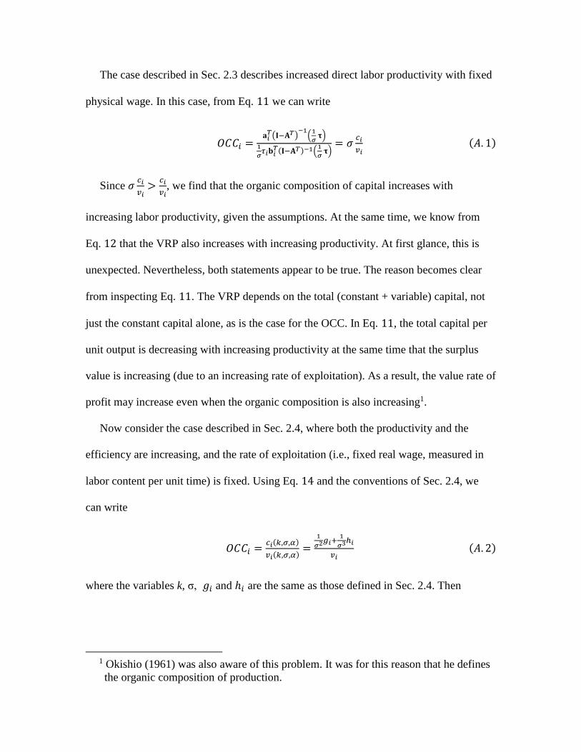
The case described in Sec. 2.3 describes increased direct labor productivity with fixed

physical wage. In this case, from Eq. 11 we can write

𝑂𝐶𝐶𝑖 =𝐚𝑖

𝑇(𝐈−𝐀𝑇)−1

(1

𝜎 𝛕)

1

𝜎𝜏𝑖𝐛𝑖

𝑇(𝐈−𝐀𝑇)−1(1

𝜎 𝛕)

= 𝜎𝑐𝑖

𝑣𝑖(𝐴. 1)

Since 𝜎𝑐𝑖

𝑣𝑖>

𝑐𝑖

𝑣𝑖, we find that the organic composition of capital increases with

increasing labor productivity, given the assumptions. At the same time, we know from

Eq. 12 that the VRP also increases with increasing productivity. At first glance, this is

unexpected. Nevertheless, both statements appear to be true. The reason becomes clear

from inspecting Eq. 11. The VRP depends on the total (constant + variable) capital, not

just the constant capital alone, as is the case for the OCC. In Eq. 11, the total capital per

unit output is decreasing with increasing productivity at the same time that the surplus

value is increasing (due to an increasing rate of exploitation). As a result, the value rate of

profit may increase even when the organic composition is also increasing1.

Now consider the case described in Sec. 2.4, where both the productivity and the

efficiency are increasing, and the rate of exploitation (i.e., fixed real wage, measured in

labor content per unit time) is fixed. Using Eq. 14 and the conventions of Sec. 2.4, we

can write

𝑂𝐶𝐶𝑖 =𝑐𝑖(𝑘,𝜎,𝛼)

𝑣𝑖(𝑘,𝜎,𝛼)=

1

𝜎2𝑔𝑖+1

𝜎3ℎ𝑖

𝑣𝑖(𝐴. 2)

where the variables k, σ, 𝑔𝑖 and ℎ𝑖 are the same as those defined in Sec. 2.4. Then

1 Okishio (1961) was also aware of this problem. It was for this reason that he defines

the organic composition of production.

𝜕

𝜕𝜎𝑂𝐶𝐶𝑖 =

−(2

𝜎3𝑔𝑖+3

𝜎4ℎ𝑖)

𝑣𝑖 < 0 (𝐴. 3)

In words, the organic composition of capital decreases with increasing productivity when

the rate of exploitation remains fixed, and the assumptions of the model are satisfied.

This is because the constant capital per unit output declines, but the wage, measured in

terms of labor content, remains fixed.

The result is different, however, in the case described in Sec. 2.5, where there is an

increase in both efficiency and productivity and the physical wage remains fixed,

allowing the rate of exploitation to increase with increasing productivity. Now, from Eqs.

19 and 21

𝑂𝐶𝐶𝑖 =1

𝜎𝑔𝑖+

1

𝜎2ℎ𝑖

𝜏𝑖(1

𝜎𝑒𝑖+

1

𝜎2𝑓𝑖)(𝐴. 4)

where the variables 𝑒𝑖, 𝑓𝑖, 𝑔𝑖, and ℎ𝑖 are the same as those defined in Sec. 2.5. Following

differentiation and rearrangement, we find that

𝜕

𝜕𝜎𝑂𝐶𝐶𝑖 =

1

𝜎[(𝑔𝑖+

1

𝜎ℎ𝑖)(

1

𝜎𝑒𝑖+

2

𝜎2𝑓𝑖)−(𝑒𝑖+1

𝜎𝑓𝑖)(

1

𝜎𝑔𝑖+

2

𝜎2ℎ𝑖)]

𝜏𝑖(1

𝜎𝑒𝑖+

1

𝜎2𝑓𝑖)2 (𝐴. 5)

Now the direction of change in the organic composition of capital per unit output is

indeterminate, given the assumptions of the model. The OCC may increase or decrease

with technical change, depending on the balance between the details of worker

consumption and (fixed and circulating) capital inputs. However, as shown by Eq. 23,

this indeterminacy is not sufficient to prevent the value rate of profit from increasing, due

to the increase in the rate of exploitation.

A.3 A temporal single-system model

The temporal single-system interpretation (TSSI) (e.g., Kliman (1996), Kliman and

McGlone (1999)); for a critical evaluation of TSSI, see e.g., Veneziani (2004), Rieu

(2009)). assumes that there is a time lag between the price of inputs and the price of

outputs. It also postulates that traditional Marxist categories, like constant capital and

surplus value must be understood in price (and not labor content) terms. That is, capital

expenses (constant capital) should be valued at historic costs (denominated in monetary

terms), while labor should be valued at current (monetary) costs. Typically, the

assumption is also made that the real wage is constant. Let us try to adopt (at least

provisionally) these assumptions into the models that we have been using in this paper.

This means, among other things that we will use labor content instead of price, and

consider VRP per unit output.

The problem arises immediately of how to incorporate time-varying costs into our

current model. If we assume that the real wage is fixed, then we need to model time-

varying constant capital. At the outset, it is worth noting that in the simple cases studied

in Secs. 2.2 and 2.3 (where only labor productivity is increased through technical

change), there is no change in the labor content of constant capital per unit output. In

other words, the historical cost and the replacement cost of fixed capital remain

unchanged per unit output. As a result, the TSSI assumption is realized trivially. In this

case, however, there is no decrease in the VRP (see Eqs. 10 and 12).

To consider the cases in which the constant capital per unit output varies as a function

of technical change (Secs. 2.4 and 2.5), assume that the constant capital historical cost is

some mixture of the old and new constant capital costs, represented by 𝑐𝑖 and 𝑐𝑖(𝑘, 𝜎, 𝛼)

respectively. Represent the temporal mixing by defining a function 𝛽(𝑡) such that

𝛽(0) = 1, and 𝛽(𝑡) declines monotonically with time to 0, where t represents clock time.

For example, 𝛽(𝑡) = 𝑒−𝛾𝑡 is one such function, where γ is a real number greater than

zero. Then if 𝛿(𝑡) = 1 − 𝛽(𝑡), the temporal mixing function may be written as

𝑐𝑖(𝑘, 𝜎, 𝛼, 𝑡) = 𝛽(𝑡)𝑐𝑖 + 𝛿(𝑡)𝑐𝑖(𝑘, 𝜎, 𝛼).

From Eqs. 14 and 15, we can write

𝑟𝑖(𝑘, 𝜎, 𝛼, 𝑡) =𝑠𝑖

𝛽(𝑡)𝜎𝑐𝑖+𝛿(𝑡)(1

𝜎𝑔𝑖+

1

𝜎2ℎ𝑖)+𝑣𝑖

(𝐴. 6)

Then after differentiation and rearrangement, we obtain

𝜕𝑟𝑖

𝜕𝜎=

𝑠𝑖(𝛿(𝑡)(1

𝜎2𝑔𝑖+2

𝜎3ℎ𝑖)−𝛽(𝑡)𝑐𝑖)

(𝛽(𝑡)𝜎𝑐𝑖+𝛿(𝑡)(1

𝜎𝑔𝑖+

1

𝜎2ℎ𝑖)+𝑣𝑖)2 (𝐴. 7)

Note the difference in the numerator between the TSSI case (Eq. 𝐴. 7) and the non-

TSSI case (Eq. 16). In particular, the time-dependence of the fixed capital cost introduces

−𝛽(𝑡)𝑐𝑖 into Eq. 𝐴. 7. This permits the value rate of profit to decline if0 𝛽(𝑡)𝑐𝑖 >

𝛿(𝑡) (1

𝜎2 𝑔𝑖 +2

𝜎3 ℎ𝑖). Whether or not this condition is satisfied depends on the balance

between several factors, whose quantitative details are not specified within the model. It

is clear, however, that there is expected to be an initial transitory decline in the value rate

of profit, since 𝛽(𝑡) ≫ 𝛿(𝑡) when t≅0. Then, since 𝛽(𝑡) tends towards 0 with increasing

time, the VRP would be expected to increase in the long-term, given the assumptions of

the model. This is not consistent with the straightforward understanding of TSSI, which

predicts a monotonic decrease in the rate of profit (e.g., Kliman and McGlone (1999)).