Teaching light scattering spectroscopy: the dimension and shape of tobacco mosaic virus

Biophysical Journal Volume 71 September 1996 1641-1650

Teaching Light Scattering Spectroscopy: The Dimension and Shape ofTobacco Mosaic Virus

Nuno C. Santos and Miguel A. R. B. CastanhoDepartamento de Quimica e Bioquimica, Faculdade de Ci6ncias da Universidade de Lisboa, Ed. Cl -5°, Campo Grande, 1700 Lisboa,and Centro de Quimica-Fisica Molecular, Complexo I, Instituto Superior T6cnico, 1096 Lisboa codex, Portugal

ABSTRACT The tobacco mosaic virus is used as a model molecular assembly to illustrate the basic potentialities of lightscattering techniques (both static and dynamic) to undergraduates. The work has two objectives: a pedagogic one(introducing light scattering to undergraduate students) and a scientific one (stabilization of the virus molecular assemblystructure by the nucleic acid). Students are first challenged to confirm the stabilization of the cylindrical shape of the virus bythe nucleic acid, at pH and ionic strength conditions where the coat proteins alone do not self-assemble. The experimentalintramolecular scattering factor is compared with the theoretical ones for several model geometries. The data clearly suggestthat the geometry is, in fact, a rod. Comparing the experimental values of gyration radius and hydrodynamic radius with thetheoretical expectations further confirms this conclusion. Moreover, the rod structure is maintained over a wider range of pHand ionic strength than that valid for the coat proteins alone. The experimental values of the diffusion coefficient and radiusof gyration are compared with the theoretical expectations assuming the dimensions detected by electron microscopytechniques. In fact, both values are in agreement (length =300 nm, radius =20 nm).

INTRODUCTION

Light scattering techniques are very easy to perform and arevery useful in studies about the structure of macromoleculesand molecular assemblies. Although its application is be-coming more common, suggestions for introductory labo-ratory work for undergraduate students are very scarce anddeal only with static light scattering (e.g., Thompson et al.,1970, Matthews, 1984, Mougain et al., 1995). We presentlaboratory work for undergraduate students where lightscattering techniques are used in multiple ways to charac-terize a molecular assembly.The tobacco mosaic virus (TMV) was the chosen model

molecular assembly because: 1) it has a very well-definedgeometry; 2) it is not spherical (due to symmetry reasons,there is a tendency to emphasize spherical geometries toomuch); 3) it is very well characterized in terms of size andshape by means of independent techniques (for a review seee.g., Caspar, 1963); and 4) it is a fairly monodispersedsystem (both size and shape).

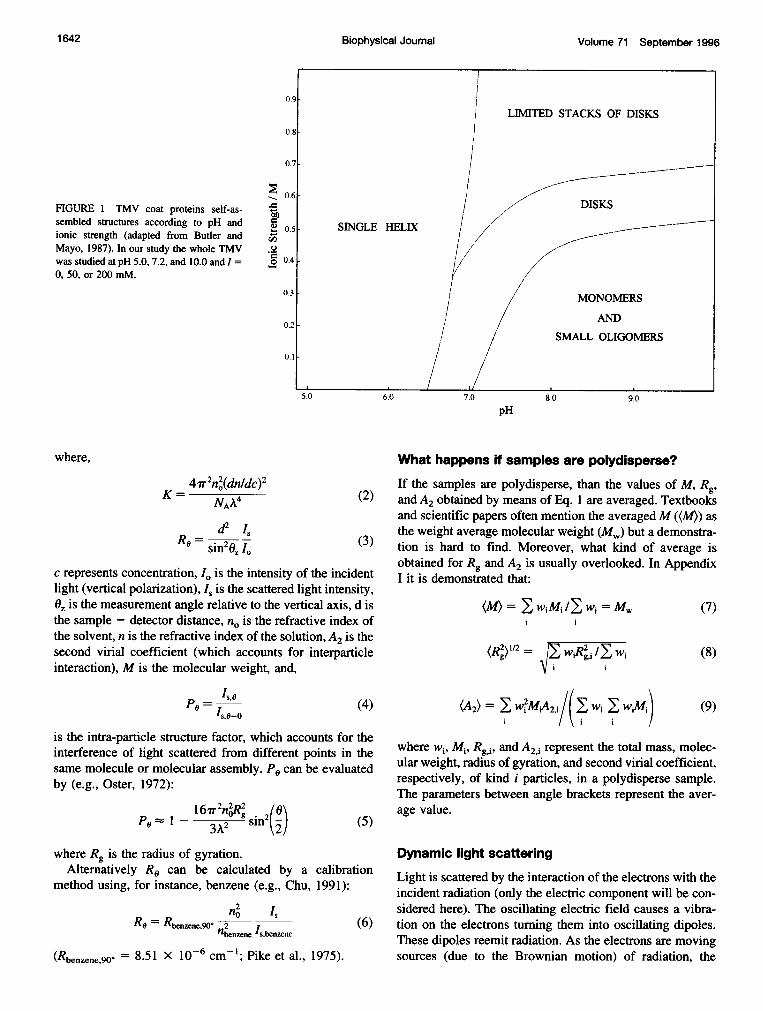
Moreover, the molecular assembly of TMV coat proteinsis largely characterized in terms of structure changes withionic strength (I) and pH (Fig. 1, e.g., Butler and Mayo,1987). According to pH and I, TMV coat proteins canremain as separated monomers, self-assemble into disks, orself-assemble into disk stacks (rods). Such dramatic struc-ture alterations are easily detected by means of light scat-tering spectroscopy techniques.

Received for publication I April 1996 and in final form 4 June 1996.Address reprint requests to Dr. Miguel A. R. B. Castanho, Centro deQuimica-Fisica Molecular, Complexo I, Instituto Superior T&cnico, 1096Lisboa codex, Portugal. Tel.: 351-1-8419248; Fax: 351-1-3524372; E-mail: [email protected] 1996 by the Biophysical Society0006-3495/96/09/1641/10 $2.00

Can the nucleic acid stabilize the cylindrical shape of thevirus in pH and I conditions where the coat proteins alonecannot? This is the first question students are challenged toanswer.

THEORETICAL BACKGROUND

Light scattering intensity is monitored either in the micro-second or in the second time range domain. This is the basicdifference between dynamic light scattering (DLS) andstatic light scattering (SLS), respectively. Fluctuations inthe intensity of light scattered by a small volume of asolution in the microsecond time range are directly relatedto the Brownian motion of the solute. Averaging the inten-sity over the second time range interval will cause a loss ofthe solute dynamic properties information; that is why lightscattering is named either static or dynamic.The outlines of the theory related to light scattering

techniques is described in biophysics (e.g., Brunner andDransfeld, 1983; Marshall, 1978), chemistry (e.g., Oster,1972), and polymer science textbooks (e.g., Munk, 1989).Introductory textbooks and review articles on light scatter-ing applications in biochemistry are also available (e.g.,Harding et al., 1992, Bloomfield, 1981). We shall onlybriefly describe some basic aspects.The light scattering intensities are recorded according to

the measurement angle (Fig. 2) and concentration.

Static light scattering

Light scattering intensity integrated over a period of time ofseconds or more varies with the measurement angle (0) andconcentration according to (Zimm, 1948):

K.c 1-=MP +2A2c (1)R0 MP0

1641

Volume 71 September 1996

FIGURE 1 TMV coat proteins self-as-sembled structures according to pH andionic strength (adapted from Butler andMayo, 1987). In our study the whole TMVwas studied at pH 5.0, 7.2, and 10.0 and I =0, 50, or 200 mM.

where,

4ii2n'(dnldc)2NAA4

2,Isi=sin2 (3)

c represents concentration, IO is the intensity of the incidentlight (vertical polarization), Is is the scattered light intensity,O is the measurement angle relative to the vertical axis, d isthe sample - detector distance, no is the refractive index ofthe solvent, n is the refractive index of the solution, A2 is thesecond virial coefficient (which accounts for interparticleinteraction), M is the molecular weight, and,

P0 Is,o

's,o=o

(4)

What happens if samples are polydisperse?

If the samples are polydisperse, than the values of M, Rg,and A2 obtained by means of Eq. 1 are averaged. Textbooksand scientific papers often mention the averagedM ((M)) as

the weight average molecular weight (Mw) but a demonstra-tion is hard to find. Moreover, what kind of average isobtained for Rg and A2 is usually overlooked. In AppendixI it is demonstrated that:

(7)

2)1/2 = WiR />J w

(A2=EWMi

(8)

(9)

is the intra-particle structure factor, which accounts for theinterference of light scattered from different points in thesame molecule or molecular assembly. Po can be evaluatedby (e.g., Oster, 1972):

16iff2n~R2PO=1- 3A2 'sin2(j) (5)

where Rg is the radius of gyration.Alternatively R. can be calculated by a calibration

method using, for instance, benzene (e.g., Chu, 1991):

n2= benzene,902 (6)

nbenzene Is,benzene

(Rbenzene,90- = 8.51 X 10V6 CM'1; Pike et al., 1975).

where wi, Mi, Rg,i, and A2i represent the total mass, molec-ular weight, radius of gyration, and second virial coefficient,respectively, of kind i particles, in a polydisperse sample.The parameters between angle brackets represent the aver-age value.

Dynamic light scattering

Light is scattered by the interaction of the electrons with theincident radiation (only the electric component will be con-sidered here). The oscillating electric field causes a vibra-tion on the electrons turning them into oscillating dipoles.These dipoles reemit radiation. As the electrons are movingsources (due to the Brownian motion) of radiation, the

5t

*a00

pH

1 642 Biophysical Journal

(M) = E wimi /E wi = Mw

Teaching Light Scattering Spectroscopy

A)

I LASER -

Cell ,0=0

-JJBeamstopper

/1

B)

LASER BEAM

Detectioncone

.A 00

8>90° 6 I

=90o

Light scattering intensity fluctuations detected in a smallvolume and in the microsecond time range (Fig. 4) arerelated to the Brownian motion of the particles due todensity fluctuations, caused by incidental agglomeration ofmolecules and variation in the number of molecules in thescattering volume. The diffusion coefficient of the solutecan be measured by means of an autocorrelation function(g2(t). (This methodology justifies the name of photoncorrelation spectroscopy sometimes used to name DLS.However, we do not think this is appropriate because sev-eral other spectroscopic methodologies can claim the samedesignation, e.g., fluorescence correlation spectroscopy isalso a photon correlation spectroscopy.) Consider It, thenumber of photons arriving at the detector at the timeinterval t'. The correlation function is built multiplying thenumber of photons from two successive time intervals andstoring the result in the first instrumental channel. Thiscalculation is repeated hundreds of thousands of times,averaged, and stored in channel 1. In the successive chan-nels the average products of It,It,+t are stored where t is thedelay time:

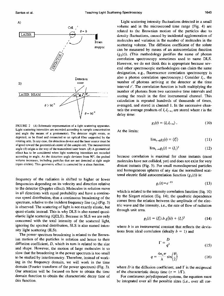
FIGURE 2 (A) Schematic representation of a light scattering apparatus.Light scattering intensities are recorded according to sample concentrationand angle (by means of a goniometer). The detector might rotate, asdepicted, or be fixed and connected to an optical fiber supported by therotating arm. In any case, the detection device and the laser source must bealigned toward the geometrical center of the sample cell. The measurementangle (0) origin is the way of the transmitted laser beam. (B) A geometricaleffect has to be considered when light scattering intensities are recordedaccording to angle. As the detection angle deviates from 90°, the probedvolume increases, including particles that are not detected at right angle(open circles). This geometric effect is corrected by a sinus function.

frequency of the radiation is shifted to higher or lowerfrequencies depending on its velocity and direction relativeto the detector (Doppler effect). Molecules in solution movein all directions with equal probability and have a continu-ous speed distribution, thus a continuous broadening of thespectrum, relative to the incident frequency line (v0) (Fig. 3)is observed. The scattering of light is not exactly elastic, butquasi-elastic instead. This is why DLS is also named quasi-elastic light scattering (QELS). Because in SLS we are onlyconcerned with the total intensity of the scattered light,ignoring the spectral distribution, SLS is also named inten-sity light scattering (ILS).The power spectrum broadening is related to the Brown-

ian motion of the particles in solution and hence to theirdiffusion coefficient, D, which in turn is related to the sizeand shape. However, the motion of large molecules is soslow that the broadening in the power spectrum is too smallto be studied by interferometry. Therefore, instead of work-ing in the frequency domain, we will work in the timedomain (Fourier transform of the power spectrum) (Fig. 3).Our attention will be focused on how to obtain the timedomain function to obtain the characteristic decay time ofthis function.

g2(t) = QI-IC+l)- (10)

At the limits:

limt-g2(t) = (i) (1 1)

limt-g2(t) = (It,)2 (12)

because correlation is maximal for close instants (mostmolecules have not collided, yet) and does not exist for verydistant instants (Fig. 5). For small monodispersed particlesand homogeneous spheres of any size the normalized scat-tered electric field autocorrelation function (gl(t)) is:

gl(t)=e-Ft (13)

which is related to the intensity correlation function (Eq. 10)by the Siegert relation (Eq. 14); the quadratic dependencecomes from the relation between the amplitude of the elec-tric wave and the intensity, i.e., the rate of flow of radiationthrough unit area.

g2(t) = (I ).b.g2(t) + (It,)2 (14)

where b is an instrumental constant that reflects the devia-tions from ideal correlation (ideally b = 1) and

DF 2

q

4noq= .inAq= A~sint (16)

where D is the diffusion coefficient, and F is the reciprocalof the characteristic decay time (T = I/F).

For continuous polydispersed systems, the equation mustbe integrated over all the possible sizes (i.e., over all cor-

(15)

1 643Santos et al.

Volume 71 September 1996

g1(t)

i/r-

g (t) = 2wr e21vt(v) dp

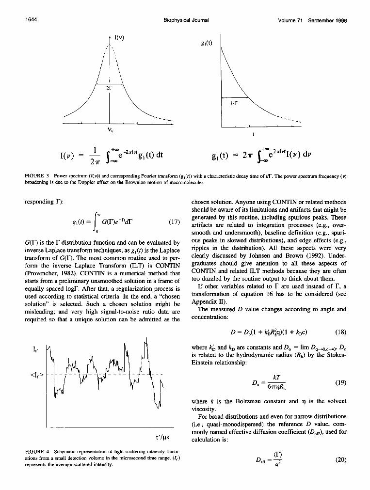
FIGURE 3 Power spectrum (I(v)) and corresponding Fourier transform (gl(t)) with a characteristic decay time of i/F. The power spectrum frequency (v)broadening is due to the Doppler effect on the Brownian motion of macromolecules.

responding F):

g(= G(F)e-rtdr (17)0

G(F) is the F distribution function and can be evaluated byinverse Laplace transform techniques, as gI(t) is the Laplacetransform of G(F). The most common routine used to per-

form the inverse Laplace Transform (ILT) is CONTIN(Provencher, 1982). CONTIN is a numerical method thatstarts from a preliminary unsmoothed solution in a frame ofequally spaced logF. After that, a regularization process isused according to statistical criteria. In the end, a "chosensolution" is selected. Such a chosen solution might bemisleading; and very high signal-to-noise ratio data are

required so that a unique solution can be admitted as the

t'/,s

FIGURE 4 Schematic representation of light scattering intensity fluctu-ations from a small detection volume in the microsecond time range. (I,,)represents the average scattered intensity.

chosen solution. Anyone using CONTIN or related methodsshould be aware of its limitations and artifacts that might begenerated by this routine, including spurious peaks. Theseartifacts are related to integration processes (e.g., over-

smooth and undersmooth), baseline definition (e.g., spuri-ous peaks in skewed distributions), and edge effects (e.g.,ripples in the distribution). All these aspects were very

clearly discussed by Johnsen and Brown (1992). Under-graduates should give attention to all these aspects ofCONTIN and related ILT methods because they are oftentoo dazzled by the routine output to think about them.

If other variables related to F are used instead of F, a

transformation of equation 16 has to be considered (seeAppendix II).The measured D value changes according to angle and

concentration:

D= Do(1 + kbR2q)(1 +kDc) (18)

where kD and kD are constants and D. = lim DqjO,cj.O D.is related to the hydrodynamic radius (Rh) by the Stokes-Einstein relationship:

kT

6inqRh (19)

where k is the Boltzman constant and is the solventviscosity.

For broad distributions and even for narrow distributions(i.e., quasi-monodispersed) the reference D value, com-

monly named effective diffusion coefficient (Deff), used forcalculation is:

Deff (20)q

I(v)

vo

I(v) = 127r

+00 -27ript (t) dtee-00

1644 Biophysical Journal

Teaching Light Scattering Spectroscopy

K3 = ((F - (F))3)

K4 = ((r - (r))4) - 3K2 (26)

(27)

K0 is the nth cumulant of gl(t). K1 is the mean of F (zaverage) and K2 is the variance of the F distribution. Theratio:

K2

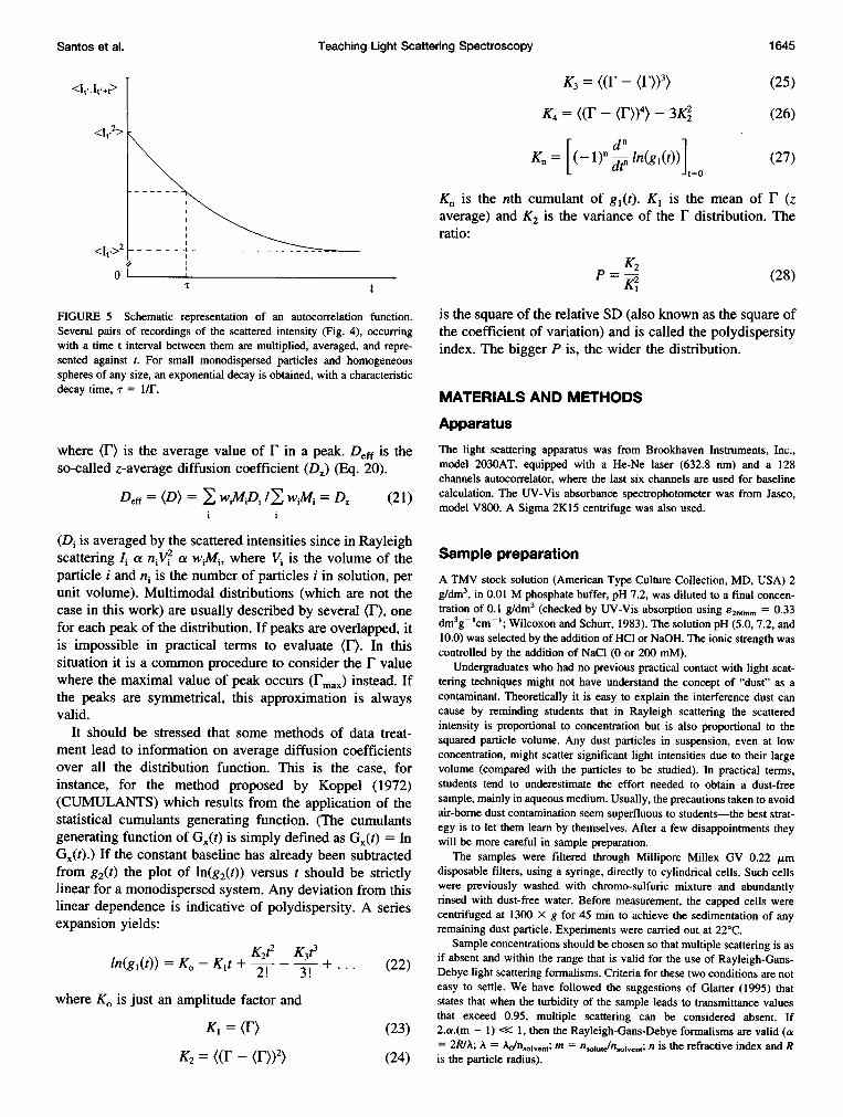
P = K2 (28)elFIGURE 5 Schematic representation of an autocorrelation function.Several pairs of recordings of the scattered intensity (Fig. 4), occurringwith a time t interval between them are multiplied, averaged, and repre-sented against t. For small monodispersed particles and homogeneousspheres of any size, an exponential decay is obtained, with a characteristicdecay time, T = 1/F.

where (F) is the average value of F in a peak. Deff is theso-called z-average diffusion coefficient (Dz) (Eq. 20).

Deff = (D) = wiMiDi /' wiMj = Dz (21)i i

(Di is averaged by the scattered intensities since in Rayleighscattering Ii a niVi2 a wiMi, where Vi is the volume of theparticle i and ni is the number of particles i in solution, perunit volume). Multimodal distributions (which are not thecase in this work) are usually described by several (F), one

for each peak of the distribution. If peaks are overlapped, itis impossible in practical terms to evaluate (F). In thissituation it is a common procedure to consider the r valuewhere the maximal value of peak occurs (.m.a) instead. Ifthe peaks are symmetrical, this approximation is alwaysvalid.

It should be stressed that some methods of data treat-ment lead to information on average diffusion coefficientsover all the distribution function. This is the case, forinstance, for the method proposed by Koppel (1972)(CUMULANTS) which results from the application of thestatistical cumulants generating function. (The cumulantsgenerating function of Gx(t) is simply defined as Gx(t) = In

Gx(t).) If the constant baseline has already been subtractedfrom g2(t) the plot of ln(g2(t)) versus t should be strictlylinear for a monodispersed system. Any deviation from thislinear dependence is indicative of polydispersity. A seriesexpansion yields:

K2t2 K3t3ln(gl(t)) = Ko-Klt+ - + * (22)

2! 3!

where Ko is just an amplitude factor and

K1 = (r) (23)

K2 = ((F - (r))2) (24)

is the square of the relative SD (also known as the square ofthe coefficient of variation) and is called the polydispersityindex. The bigger P is, the wider the distribution.

MATERIALS AND METHODS

ApparatusThe light scattering apparatus was from Brookhaven Instruments, Inc.,model 2030AT, equipped with a He-Ne laser (632.8 nm) and a 128channels autocorrelator, where the last six channels are used for baselinecalculation. The UV-Vis absorbance spectrophotometer was from Jasco,model V800. A Sigma 2K15 centrifuge was also used.

Sample preparationA TMV stock solution (American Type Culture Collection, MD, USA) 2g/dm3, in 0.01 M phosphate buffer, pH 7.2, was diluted to a final concen-tration of 0.1 g/dm3 (checked by UV-Vis absorption using 6260nm = 0.33dm3g- cm-'; Wilcoxon and Schurr, 1983). The solution pH (5.0, 7.2, and10.0) was selected by the addition of HCl or NaOH. The ionic strength wascontrolled by the addition of NaCl (0 or 200 mM).

Undergraduates who had no previous practical contact with light scat-tering techniques might not have understand the concept of "dust" as acontaminant. Theoretically it is easy to explain the interference dust cancause by reminding students that in Rayleigh scattering the scatteredintensity is proportional to concentration but is also proportional to thesquared particle volume. Any dust particles in suspension, even at lowconcentration, might scatter significant light intensities due to their largevolume (compared with the particles to be studied). In practical terms,students tend to underestimate the effort needed to obtain a dust-freesample, mainly in aqueous medium. Usually, the precautions taken to avoidair-borne dust contamination seem superfluous to students-the best strat-egy is to let them learn by themselves. After a few disappointments theywill be more careful in sample preparation.

The samples were filtered through Millipore Millex GV 0.22 ,umdisposable filters, using a syringe, directly to cylindrical cells. Such cellswere previously washed with chromo-sulfuric mixture and abundantlyrinsed with dust-free water. Before measurement, the capped cells were

centrifuged at 1300 X g for 45 min to achieve the sedimentation of anyremaining dust particle. Experiments were carried out at 22°C.

Sample concentrations should be chosen so that multiple scattering is asif absent and within the range that is valid for the use of Rayleigh-Gans-Debye light scattering formalisms. Criteria for these two conditions are noteasy to settle. We have followed the suggestions of Glatter (1995) thatstates that when the turbidity of the sample leads to transmittance valuesthat exceed 0.95, multiple scattering can be considered absent. If2.a.(m - 1) << 1, then the Rayleigh-Gans-Debye formalisms are valid (a= 2RIA; A = /nsolvent; m = nsolute/nsoivent; n is the refractive index and Ris the particle radius).

<it,2>

<It0>2oI-

(25)

T t

Santos et al. 1645

4

d n

K. = (- I)n ln(gl(t))din t=O

Volume 71 September 1996

Data treatment

Although the software packages of most light scattering apparatus includean automatic SLS data treatment to calculate Mw, A2, and Rg, using theZimm method, it is convenient that undergraduate students calculate theseparameters step by step. This is the only way toward a complete under-standing of the reasons beyond it. Otherwise, these parameters will be theresult of a "black box." The concentration dependence in the range studiedis negligible (Johnson and Brown, 1992) and so, even for the sake ofsimplicity and time management, we have admitted that A2 = 0. Never-theless, the methodology is very well demonstrated with Rg and Mw, only.

Equation 1 can be reformulated into:

1 A A 167n,lR2 .21O\Is + M A in2 hI (29)

where A is a constant. Plotting I/I, against sin2(0/2) for low angles, a linearrelationship is expected. Dividing the slope by the intercept, Rg can becalculated:

Slope 16iT 2n2R2Intercept 3A23

Once Rg is known, and assuming that dn/dc of TMV at 536 nm (0.184cm3g-') (Huglin, 1989) is not significantly different from the one wewould measure at 632.8 nm (an accurate measurement at 632.8 nm wasprevented by the very low concentration of TMV used), then M" can beobtained from Eq. 1 using the extrapolated data to q = 0 (zero angleconditions). The concentration dependence of D is also negligible in theconditions studied (Sano, 1987). This means kD = 0 in Eq. 18 and thus Do= limqOD.

RESULTS

Dynamic light scattering

The size distribution function obtained at low angle are allfairly monodispersed and this characteristic is maintainedregardless of pH and I. An example is depicted in Fig. 6.The extrapolated D values to q2 = 0 (Do) are shown in

Table 1, along with the corresponding Rh. The depictedvalues were obtained from (r) (CONTIN) but Do valuesobtained from the CUMULANTS method are similar.

TABLE I Radius of gyration (R.), hydrodynamic radius (Rh),diffusion coefficient at zero angle conditions (D.), and weightaverage molecular weight of TMV at several pH and ionicstrengths (I)

mol wtpH I/mM Rg/nm Rh/nm D. x 108/cm2 s-I 10-6/g mol-

5.0 0 98.4 55 4.0 21.350 108.8 51 4.3 18.3

200 94.8 55 4.0 18.87.2 0 113.6 55 3.9 26.3

50 103.1 51 4.2 23.5200 109.4 55 3.9 25.1

10.0 0 99.1 51 4.2 21.150 92.6 51 4.3 22.9

200 105.6 51 4.2 31.2

Static light scattering

The 1/II vs. sin2(0/2) data were fitted by second degreepolynomial functions. The residuals and x2 parameters wereused to decide about the goodness of the fit. The fits weresatisfactory in any case. Fig. 7 is an example (pH 7.2, I =0 mM). Rg was calculated from the tangent to the seconddegree polynomial (ax2 + bx + c) at zero angle (bx + c).Rg values are listed in Table 1 for the conditions studied.The corresponding values of Mw are also listed.

The experimental particle structure factor, Pq, is simply,

c

Pq = aX2 + bx + c (31)

which results directly from Eq. 4. Students tend to overlookthe very simple definition of Pq (Eq. 4) and remember Eq.5 only. It is noteworthy to stress that if we were dealing withconcentration-dependent data, then Eq. 31 would be validonly for zero concentration (infinite dilution) extrapolateddata.

8

0.5

I

r1. - 1.51.0 1.5

.0\ - - .5

2.0 2.5 3.0

Log (Rh/nm)

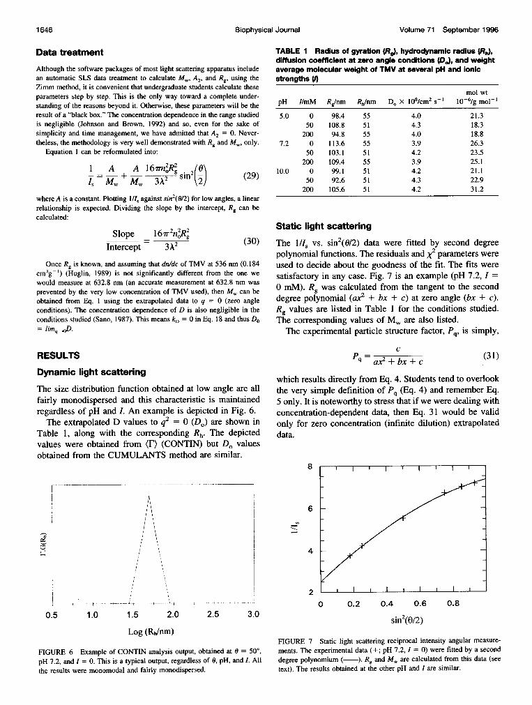
FIGURE 6 Example of CONTIN analysis output, obtained at 0 = 50°,pH 7.2, and I = 0. This is a typical output, regardless of 0, pH, and I. All

the results were monomodal and fairly monodispersed.

6

4

20 0.2 0.4 0.6 0.8

sin2(0/2)

FIGURE 7 Static light scattering reciprocal intensity angular measure-

ments. The experimental data (+; pH 7.2, 1 = 0) were fitted by a seconddegree polynomium ( ). Rg and MW are calculated from this data (seetext). The results obtained at the other pH and I are similar.

Biophysical Journal1 646

Teaching Light Scattering Spectroscopy

DISCUSSION

None of the parameters studied seem to vary significantlywith pH or I. The nucleic acid nucleic stabilizes the virusstructure over a wider range of pH and I than those valid forthe coat proteins alone (Fig. 1; for a review on coat proteinassemblies alone see e.g., Buttler and Mayo, 1987). How-ever, is this structure the cylinder that students are used toseeing on textbooks?The first approach to solve this new problem can be to

compare the experimental intraparticle static structure factor(named either Pq or P.) with the theoretical expectation forsome of the more common geometry models.

Comparing experimental and theoretical PqThe theoretical expectations for Pq according to each ofseveral model geometries are quite complex. Eqs. 32-34represent the theoretical expectations for a sphere (radius,R), infinitely thin rod (length, L), and Gaussian coil, respec-tively (e.g., Schmitz, 1990).

Pq(q.R) = {(qR)3 [sin(qR) - q.R.cos(q.R)]} (32)

2 q SinZ 2 si q.L\]2Pq(q.L) L J Z -[qL2-) (33)

22Pq(q.Rg) = (Rg)4 [exp(-q2.Rg) + (q.Rg)2 - 1] (34)

Some handbooks have long lists of Pq versus q.Rg forseveral geometries (e.g., Casassa, 1989). Nevertheless, suchhandbooks are not common in most laboratories. That iswhy we present the following polynomial equations thatresult from fitting a fifth degree polynomium to the Pqversus q.Rg data. Eqs. 35-37 correspond to the same threegeometries referred above (sphere, thin rod, and randomcoil, respectively):

Pq(q.Rg) = 0.9977 + 0.0366qRg - 0.4396(qRg)2(35)

+ 0. 1072(qRg)3 + 0.0 IIl(qRg)4 -0.038(qRg)5

Pq(q.Rg) = 0.9954 + 0.0837qRg - 0.6068(qRg)2(36)

+ 0.3220(qRg)3 - 0.0656(qRg)4 + 0.0046(qRg)5

Pq(q.Rg) = 0.9971 + 0.0579qRg - 0.5388(qRg)2(37)

+ 0.2669(qRg)3 - 0.0520(qRg)4 + 0.036(qRg)5

In these equations the parameters have no physical meaningbecause they result from a fit that is only intended tosubstitute the meaningful, but rather complex, originalequations by simple, useful, and easy to handle equations.The deviations between fitted and "real" values are always

<1% for values of qRg <2.3, 2.4, and 3.2, for a coil, sphere,and rod, respectively (data not shown).

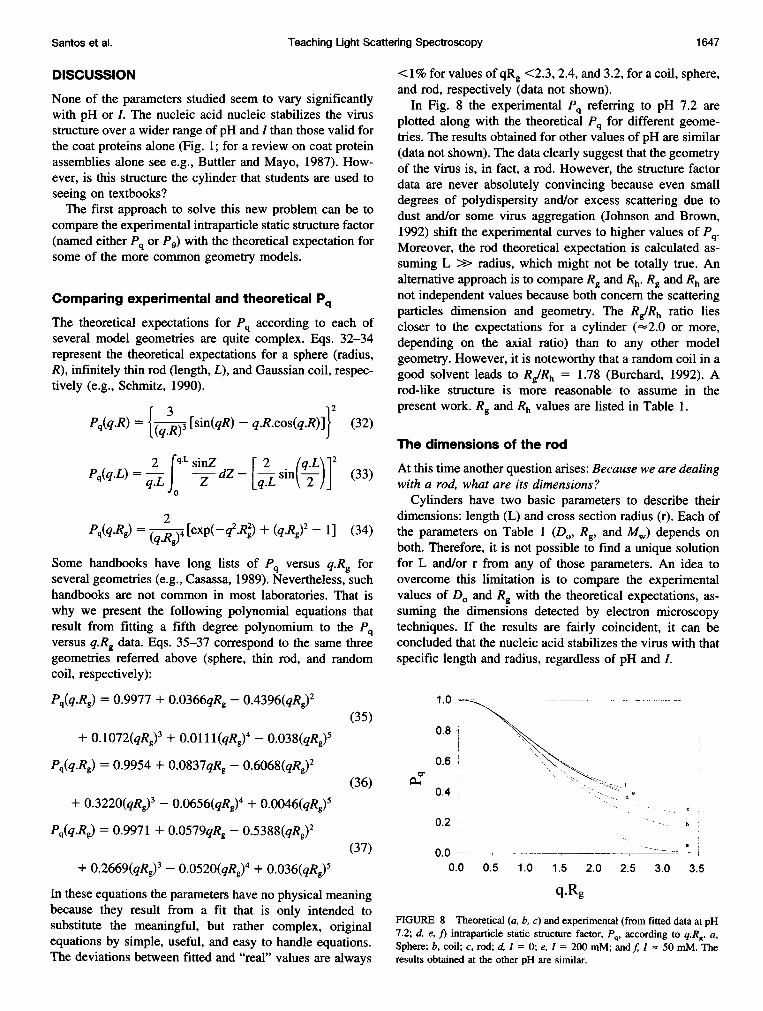
In Fig. 8 the experimental Pq referring to pH 7.2 areplotted along with the theoretical Pq for different geome-tries. The results obtained for other values of pH are similar(data not shown). The data clearly suggest that the geometryof the virus is, in fact, a rod. However, the structure factordata are never absolutely convincing because even smalldegrees of polydispersity and/or excess scattering due todust and/or some virus aggregation (Johnson and Brown,1992) shift the experimental curves to higher values of Pq.Moreover, the rod theoretical expectation is calculated as-suming L >> radius, which might not be totally true. Analternative approach is to compare Rg and Rh. Rg and Rh arenot independent values because both concern the scatteringparticles dimension and geometry. The RglRh ratio liescloser to the expectations for a cylinder (--2.0 or more,depending on the axial ratio) than to any other modelgeometry. However, it is noteworthy that a random coil in agood solvent leads to Rg/Rh = 1.78 (Burchard, 1992). Arod-like structure is more reasonable to assume in thepresent work. Rg and Rh values are listed in Table 1.

The dimensions of the rod

At this time another question arises: Because we are dealingwith a rod, what are its dimensions?

Cylinders have two basic parameters to describe theirdimensions: length (L) and cross section radius (r). Each ofthe parameters on Table 1 (Dog Rg, and Mw) depends onboth. Therefore, it is not possible to find a unique solutionfor L and/or r from any of those parameters. An idea toovercome this limitation is to compare the experimentalvalues of Do and Rg with the theoretical expectations, as-suming the dimensions detected by electron microscopytechniques. If the results are fairly coincident, it can beconcluded that the nucleic acid stabilizes the virus with thatspecific length and radius, regardless of pH and I.

1.0

a,

0.8

0.6 I

0.4 ,

0.2

0.00.0 0.5 1.0 1.5 2.0 2.5 3.0 3.5

q.Rg

FIGURE 8 Theoretical (a, b, c) and experimental (from fitted data at pH7.2; d, e, f) intraparticle static structure factor, Pq, according to q.Rg. a,Sphere; b, coil; c, rod; d, I = 0; e, I = 200 mM; andf I = 50 mM. Theresults obtained at the other pH are similar.

I~~~~~~~~~~~~~~~~~~~~~~~~~~~~~~~~~~

Santos et al. 1647

e

b

Volume 71 September 1996

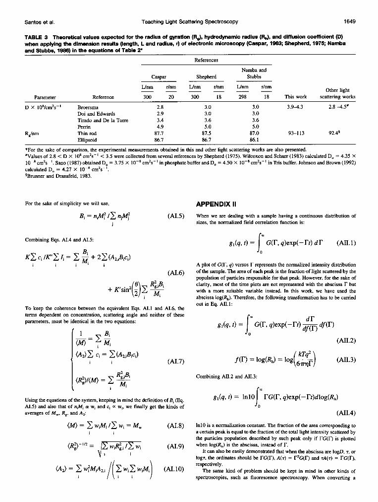
The theoretical expectations are listed in Table 2 and theresults are listed in Table 3. The experimental values of D.suggest we are dealing with cylinders having similar dimen-sions to the ones detected by electron microscopy techniques.Not surprisingly Rg values are slightly higher than ex-

pected, probably due to the small but effective fraction ofpolydispersity and/or presence of trace amounts of dustand/or some end-to-end virus aggregation. The slightlyoverestimated Rg are a direct consequence from the "up-ward" shifts of experimental Pq relative to theoretical Pq.Nevertheless, our measurements are in agreement with apreviously published result (Table 3).The molecular weights evaluated by light scattering (Ta-

ble 1) are compatible with the value of (40 ± 1) X 106(Boedtker and Simmons, 1958; Weber et al., 1963), 39.4 X106 + 2% referred by Caspar (1963), and 40.8 X 106obtained from combining DLS and sedimentation data(Johnson and Brown, 1992). The translational diffusioncoefficients calculated in this work are in close agreementwith those available in the literature for TMV (see Table 3).

CONCLUSIONS

After data analysis and treatment, undergraduate studentscan easily conclude that: 1) The geometry of the TMV isinvariant with pH (5.0-10.0) and I (0-200 mM); 2) thegeometry of the TMV is a cylinder, and 3) the virus dimen-sions are L 300 nm and r 20 nm. The basic principles

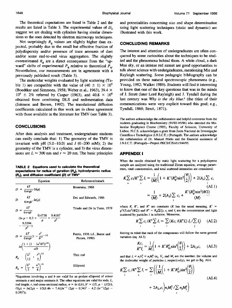
TABLE 2 Equations used to calculate the theoreticalexpectations for radius of gyration (Rg), hydrodynamic radius(RJ, and diffusion coefficient (D) of TMV*

Equation Reference/remark

kT (p) Broersma, 1960

kT Doi and Edwards, 1986D = 6'r'b ln(p)

kT Tirado and De la Torre, 19796rr'qb'

0.4738 0.4167(lnp+0.3+ + p2

p0.3394

p3kT a( /2 Perrin, 1936 (cf., Beme and

6rTqb b2 Pecora, 1990)

i1 + (1-a2/b2))1'2alb J

R L2 +2)1/2 Thin rodRg = V- + -J

(b2 a2 1/2 EllipsoidRg = V- + -J

*Equations involving a and b are valid for an prolate ellipsoid of minorsemiaxis a and major semiaxis b. The other equations are valid for rods. L,rod length; r, rod cross-sectional radius, oa = In (L/r), b' 112, p = LJ(2r),G(p) = In(2p) - 1/2(1.46 - 7.4((1n-' (2p) - 0.34)2 _ 4.2 (In-'(2p) -

and potentialities concerning size and shape determinationusing light scattering techniques (static and dynamic) are

illustrated with this work.

CONCLUDING REMARKS

The interest and attention of undergraduates are often con-

quered by some curiosities about the techniques to be stud-ied and the phenomena behind them. A white cloud, a darkblue sky, or an intense red sunset are good opportunities totalk about science with undergraduates, mentioning Mie andRayleigh scattering. Some pedagogic bibliography can beprovided on these natural spectroscopic phenomena (e.g.,Young, 1982; Walker 1989). Students will find it interestingto know that one of the key questions that was in the mindsof J. Strutt (later Lord Rayleigh) and J. Tyndall during thelast century was Why is the sky blue? (the titles of theircommunications were very explicit toward this goal; e.g.,

Tyndall, 1869; Strutt, 1871).

The authors acknowledge the collaboration and helpful comments from thestudents graduating in Biochemistry (91/92-95/96) who attended the Mo-lecular Biophysics Course (1995), Faculty of Sciences, University ofLisbon. N.C.S. acknowledges a grant from Junta Nacional de Investiga,coCientifica e Techol6gica (J.N.I.C.T.) (Portugal). The authors acknowledgethe collaboration of Dr. Manuel Prieto and the financial assistance ofJ.N.I.C.T. (Portugal)-Project PECS/C/SAU/144/95.

APPENDIX I

When the results obtained by static light scattering for a polydispersesample are analyzed using the traditional Zimm equation, average param-eters, total concentration, and total scattered intensities are considered:

KY, ci/K'>: =(I (1 + K'(Rg)sin2(2)) + 2(Az) ci

(AI. 1)1 ( )E K'(R2)sin2(0/2)

+ 2(A2)>: ci +

where K, K', and K' are constants (K has the usual meaning, K' =

q2/(3.sin2(O/2)) and K' = R/I2), ci and Ii are the concentration and lightscattered by particles i in solution. Moreover,

KE ci IK"E Ii = E (Kci /(K"I) Ii / Ij) (AI.2)i i i j

Having in mind that each of the components will follow the same generalvariation (eq. AI.3)

Kc = 1-1 + K'R22sin2(0) +2A2,ciK'Il Ml

(AI.3)

and that IA a njVj2 oc n1M2j (n1, Vi, and M1 are the number, the volume andthe molecular weight of particles i, respectively), we get to Eq. AI.4.

KY, ci IK" I, =E(( I1+K'R2.sin2i i i

(AI.4)

+ 2A2 iCi0.39)2)).

1 648 Biophysical Journal

Teaching Light Scattering Spectroscopy

TABLE 3 Theoretical values expected for the radius of gyration (R.), hydrodynamic radius (Rh), and diffusion coefficient (D)when applying the dimension results (length, L and radius, r) of electronic microscopy (Caspar, 1963; Shepherd, 1975; Nambaand Stubbs, 1986) in the equations of Table 2*

References

Namba andCaspar Shepherd Stubbs

L/nm r/nm L/nm r/nm L/nm r/nm Other lightParameter Reference 300 20 300 18 298 18 This work scattering works

D X 108/cm2s-I Broersma 2.8 3.0 3.0 3.9-4.3 2.8 -45#Doi and Edwards 2.9 3.0 3.0Tirado and De la Torre 3.4 3.6 3.6Perrin 4.9 5.0 5.0

Rg/nm Thin rod 87.7 87.5 87.0 93-113 92.40Ellipsoid 86.7 86.7 86.1

*For the sake of comparison, the experimental measurements obtained in this and other light scattering works are also presented.#Values of 2.8 < D X 108 cm2s ' < 3.5 were collected from several references by Shepherd (1975). Wilcoxon and Schurr (1983) calculated D. = 4.35 X

10-8 cm2s- l. Sano (1987) obtained D. = 3.75 X 10-8 cm2s- I in phosphate buffer and D. = 4.50 X 10-8 cm2s- I in Tris buffer. Johnson and Brown (1992)calculated Do = 4.27 X 10-8 cm2s- 1.*Brunner and Dransfeld, 1983.

For the sake of simplicity we will use,

B = n M2./>njM (AI.5)

Combining Eqs. AI.4 and AI.5:

K>: ci IK", I, = >: - + 2E (A2jiBjcj)i i i i i

(AI.6)

R22 MBi+ K'sin2(2) 9,B

To keep the coherence between the equivalent Eqs. AI.1 and AI.6, theterms dependent on concentration, scattering angle and neither of theseparameters, must be identical in the two equations:

1 E B(M) i MA(A2)E =Ci (A2,iBic1)

i i (AI.7)

(R2)/(M)= 92

Using the equations of the system, keeping in mind the definition of Bi (Eq.AI.5) and also that of niM, a w1 and c; X wi, we finally get the kinds ofaverages of MW, Rg, and A2:

(M) WAM /Ewi=Mw (AI.8)i

(Rg) w g i/ w, (AI.9)Wi i

(A2) =EWi2MiA2i /( wiE wiMj) (AI.1O)

APPENDIX 11

When we are dealing with a sample having a continuous distribution ofsizes, the normalized field correlation function is:

gl(q,t) = G(F, q)exp(-]Ft) dF0

(AII.1)

A plot of G(F, q) versus F represents the normalized intensity distributionof the sample. The area of each peak is the fraction of light scattered by thepopulation of particles responsible for that peak. However, for the sake ofclarity, most of the time plots are not represented with the abscissa F butwith a more suitable variable instead. In this work, we have used theabscissa log(Rh). Therefore, the following transformation has to be carriedout in Eq. AII.1:

("a dIFgl(q, t) = J G(F, q)exp(-Ft) df(F) df(r)

(AII.2)

l kTq2f(r) = log(Rh) = log6ii (AII.3)

Combining AH.2 and AII.3:

x

g,(q, t) = InlOf FG(F, q)exp(-Ft)dlog(Rh)

(AII.4)lnlO is a normalization constant. The fraction of the area corresponding toa certain peak is equal to the fraction of the total light intensity scattered bythe particles population described by such peak only if FG(F) is plottedwhen log(Rh) is the abscissa, instead of r.

It can also be easily demonstrated that when the abscissa are logD, T, orlogT, the ordinates should be FG(r), A(T) = r2G(r) and TA(T) = rG(r),respectively.

The same kind of problem should be kept in mind in other kinds ofspectroscopies, such as fluorescence spectroscopy. When converting a

Santos et al. 1649

1650 Biophysical Journal Volume 71 September 1996

spectrum in wavelength (A) to frequencies or wavenumbers (v), for in-stance, it may take more than only converting the abscissa. If If representsthe fluorescence intensity, then

[A2 V2 M

IfdA = If(dAlddv = JIfv- dv.JAI VI V2

Such problem does not exist in an absorption spectrum, where relativemeasurements are carried out, canceling all the needed correction terms inthe data analysis.

REFERENCES

Beme, B. J. and R. Pecora. 1990. Dynamic Light Scattering with Appli-cations to Chemistry, Biology and Physics. Robert E. Krieger Pub. Co.,Malabar. 143-144.

Bloomfield, V. A. 1981. Quasi-elastic light-scattering in biochemistry andbiology. Annu. Rev. Biophys. Bioeng. 10:421-450.

Boedtker, H. and N. S. Simmons. 1958. The preparation and characteriza-tion of essentially uniform tobacco mosaic virus particles. J. Am. Chem.Soc. 80:2550-2556.

Broersma, S. 1960. Rotational diffusion constant of a cylindrical particle.J. Chem. Phys. 32:1626-1635.

Brunner, H. and K. Dransfeld. 1983. Light scattering by macromolecules.In Biophysics, W. Hoppe, W. Lohmann, H. Markl, and H. Ziegler,editors. Springer-Verlag, New York. 93-100.

Burchard, W. 1992. Static and dynamic light scattering approaches tostructure determination of biopolymers. In Laser Light Scattering inBiochemistry. S. E. Harding, D. B. Sattelle, and V. A. Bloomfield,editors. Royal Society of Chemistry, Cambridge. 3-22.

Butler, P. J. G. and M. A. Mayo. 1987. Molecular architecture andassembly of tobacco mosaic virus particles. In The molecular biology ofthe positive strand RNA viruses. Academic Press Inc., London.237-257.

Casassa, E. F. 1989. Particle scattering factors in Rayleigh scattering. InPolymer Handbook. J. Brandup and E. H. Immergut, editors. John Wiley& Sons, New York. VII/485-491.

Caspar, D. L. D. 1963. Assembly and stability of the tobacco mosaic virusparticle. Adv. Protein Chem. 18:37-121.

Chu, B. 1991. Laser Light Scattering. Basic Principles and Practice. Aca-demic Press, New York. 13-20.

Doi, M. and S. F. Edwards. 1986. The Theory of Polymer Dynamics.Oxford University Press, Oxford. 289-323.

Glatter, 0. 1995. Modem methods of data analysis in small-angle scatter-ing and light scattering. In Modem Aspects of Small-Angle Scattering.H. Brumberger, editor. Kluwer Academic Publishers, Dordrecht.107-180.

Harding, S. E., D. B. Sattelle, and V. A. Bloomfield. 1992. Laser LightScattering in Biochemistry. Royal Society of Chemistry, Cambridge.

Huglin, M. B. 1989. Specific refractive index increments of polymers indilute solutions. In Polymer Handbook. J. Brandrup and E. H. Immergut,editors. John Wiley & Sons, New York. VII/409-484.

Johnsen, R. and W. Brown. 1992. An overview of current methods ofanalyzing QLS data. In Laser Light Scattering in Biochemistry. S. E.Harding, D. B. Sattelle, and V. A. Bloomfield, editors. Royal Society ofChemistry, Cambridge. 77-91.

Johnson, P. and W. Brown. 1992. An investigation of rigid rod-likeparticles in dilute solution. In Laser Light Scattering in Biochemistry. S.E. Harding, D. B. Sattelle, and V. A. Bloomfield, editors. Royal Societyof Chemistry, Cambridge. 161-183.

Koppel, D. E. 1972. Analysis of macromolecular polydispersity in intensitycorrelation spectroscopy: the method of cumulants. J. Chem. Phys.57:4814-4820.

Marshall, A. G. 1978. Biophysical Chemistry: Principles, Techniques andApplications. John Wiley & Sons, New York. 463-503.

Matthews, G. P. 1984. Light Scattering by Polymers. Two Experiments forAdvanced Undergraduates. J. Chem. Educ. 61:552-554.

Mougan, M. A., A. Coello, F. Meijide, and J. V. Tato. 1995. Spectrofluo-rimeters as light scattering apparatus. Application to polymers molecularweight determination. J. Chem. Educ. 72:284-286.

Munk, P. 1989. Introduction to Macromolecular Science. John Wiley &Sons, New York. 375-400.

Namba, K. and G. Stubbs. 1986. Structure of tobacco mosaic virus at 3.6A resolution: implications for assembly. Science. 231:1401-1406.

Oster, G. 1972. Light Scattering. In Techniques of Chemistry, Vol. I, PartIRA. A. Weissberger and B. W. Rossiter, editors. Wiley-Interscience,New York. 75-117.

Perrin, F. 1936. Brownian movement of an ellipsoid. II. Free rotation anddepolarization of fluorescence. Translation and diffusion of ellipsoidalmolecules. J. Phys. Radium. 7:1-11.

Pike, E. R., W. R. M. Pomeroy, and J. M. Vaughan. 1975. Measurement ofRayleigh ratio for several pure liquids using a laser and monitoredphoton counting. J. Chem. Phys. 62:3188-3192.

Provencher, S. W. 1982. A constrained regularization method for invertingdata represented by linear algebraic or integral equations. Comput. Phys.Commun. 27:213-227.

Sano, Y. 1987. Translational diffusion coefficient of tobacco mosaic virusparticles. J. Gen. Virol. 68:2439-2442.

Schmitz, K. S. 1990. An Introduction to Dynamic Light Scattering byMacromolecules. Academic Press, San Diego. 22.

Shepherd, I. W. 1975. Inelastic laser light scattering from synthetic andbiological polymers. Rep. Prog. Phys. 38:565-620.

Strutt, J. W. 1871. On the light from the sky, its polarization and color.Phil. Mag. 41:107-120, 274-279.

Thompson, A. C., K. G. Kozimer, and D. Stockwell. 1970. A lightscattering experiment for physical chemistry. J. Chem. Educ. 47:828-831.

Tirado, M. M. and J. G. De la Torre. 1979. Translational friction coeffi-cients of rigid, symmetric top macromolecules. Application to circularcylinders. J. Chem. Phys. 71:2581-2587.

Tyndall, J. 1869. On the blue color of the sky, the polarization of skylightand the polarization of light by cloudy matter generally. Phil. Mag.37:384-394.

Walker, J. 1989. The colors seen in the sky offer lessons in opticalspectroscopy. Sci. Am. 260:84-87.

Weber, F. N., Jr., R. M. Elton, H. G. Kim, R. D. Rose, R. L. Steere, andD. W. Kupke. 1963. Equilibrium sedimentation of uniform rods oftobacco mosaic virus. Science. 140:1090-1092.

Wilcoxon, J. and J. M. Schurr. 1983. Dynamic light scattering from thinrigid rods: anisotropy of translational diffusion of tobacco mosaic virus.Biopolymers. 22:849-867.

Young, A. T. 1982. Rayleigh scattering. Phys. Today. 35:42-48.Zimm, B. H. 1948. Apparatus and methods for measurement and interpre-

tation of the angular variation of light scattering; preliminary results onpolystyrene solutions. J. Chem. Phys. 16:1099-1116.