TDOA Source-Localization Technique Robust to Timing Attacks

1

TDOA Source-Localization Technique Robust toTiming Attacks

Marguerite Delcourt Student Member, IEEE, Jean-Yves Le Boudec Fellow, IEEE

Abstract—In this paper, we focus on the localization of apassive source from time difference of arrival (TDOA) measure-ments. TDOA values are computed with respect to pairs of fixedsensors that are required to be accurately time-synchronized.This constitutes a weakness as all synchronization techniquesare vulnerable to delay injections. Attackers are able eitherto spoof the signal or to inject asymmetric delays in thecommunication channel. By nature, TDOA measurements arehighly sensitive to time-synchronization offsets between sensors.Our first contribution is to show that timing attacks can severelyaffect the localization process. With a delay of a few microsecondsinjected on one sensor, the resulting estimate might be severalkilometers away from the true location of the unknown source.We also show that residual analysis does not enable the detectionand identification of timing attacks. Our second contributionis to propose a two-step TDOA-localization technique that isrobust against timing attacks. It uses a known source to define aweight for each pair of sensors, reflecting the confidence in theirtime synchronization. Our solution then uses the weighted least-squares estimator with the newly created weights and the TDOAmeasurements received from the unknown source. As a result,our method either identifies the network as being too corrupt tolocalize, or gives a corrected estimate of the unknown positionalong with a confidence metric. Numerical results illustrate theperformance of our technique.

I. INTRODUCTION

The problem of localizing uncooperative sources that emitradio frequency signals has been extensively studied in thefield of electronic warfare [1], as well as for civil applica-tions [2]. Solutions were proposed in various settings such assensor networks, radar, sonar or wireless communication [3]–[5]. Localization methods rely on the timely analysis of mea-surements such as angles of arrival (AOA), time differencesof arrival (TDOA) between sensors, frequency differences ofarrival (FDOA) between sensors or a combination of them [1],[6], [7]. Therefore, an accurate synchronization of the timereference between sensors is essential. This can be achievedvia satellite positioning systems or through packet-based pro-tocols such as WhiteRabbit [8]. However, both techniques arevulnerable to timing attacks, which constitutes a weaknessfor localization systems. Attackers are able either to spoofthe signal [9] or to insert a delay box on the links usedfor the synchronization communication [10]. Such a delaybox modifies asymmetrically the length of the communicationpaths, which indirectly injects delays in the time reference ofsensors. The transmitted synchronization data is untouched by

M. Delcourt and J-Y. Le Boudec are with the School of Computerand Communication Sciences of the Swiss Federal Institute of Tech-nology Lausanne, EPFL, Switzerland. e-mail: {marguerite.delcourt| jean-yves.leboudec}@epfl.ch.

the attacker, hence it still satisfies all cryptographic securityrequirements in place such as authentication, integrity orconfidentiality. A timing attack produces positive or negativeoffsets between the time reference of the sensors. The contentof the data received and transmitted by the sensors alsoremains protected by the traditional cybersecurity protocols.The only noticeable effect of such an attack is if it affectsthe function of the system. Specifically, if it does not resultin a misestimation of the location, then it is not detectable.Furthermore, an undetectable attack is required to be acceptedand implemented by the clock controller of the sensors, a toolarge delay is flagged and raises suspicion. This is achieved byinjecting small and gradually increasing delays. Although theyrequire tampering with the communication network, timingattacks do not require any physical access to the potentiallyguarded sensors. Observe that it is realistic to assume non-guarded links between protected sensors.

In this paper, we focus on the TDOA-based localizationof a passive source from a network of fixed sensors whosetime references could be maliciously manipulated. TDOAmeasurements offer high precision hence are widely used.However, they are easily attacked because they are particularlysensitive to timing errors. Due to the high propagation speedof the signal, a small synchronization error can lead to alarge range difference error between the two sensors and thesource. For example, if 3µs are added to a TDOA measure-ment, then the corresponding range difference is increasedby approximately 900m. Consequently, an attacked networkcould become unable to localize sources or an attacked vehiclecould unintendedly enter on a wrong territory. Note that timingattacks are also a threat to other types of networks. Forexample, the control and operation of Smart Grids require anunderstanding of the system state at specific time intervals. Itwas shown that undetectable timing attacks on grid sensorsare feasible and that they can lead to an incorrect stateestimation, which in turn can result in a blackout or in assetdegradation [11].

Our first contribution is to study the effect of timing attackson the TDOA-based localization of an unknown source. Weshow that the delays between sensors can lead to a misestima-tion of the source location. We inject a few microseconds intoone sensor and obtain an estimate that is approximately 1 kmaway from the true position of the source. We further explainhow an attacker can compute positive or negative delays suchthat the localization process results in a specifically chosenmisestimation. We also show that residual analysis does notenable the detection and identification of timing attacks.

Our second contribution is to propose a TDOA-localization

arX

iv:1

912.

0463

0v1

[ee

ss.S

Y]

10

Dec

201

9

2

technique that is robust against timing attacks. It works in twophases, the first analyses the error in TDOA measurements re-ceived from a known calibration source. As a result, it definesa weight for each pair of sensors; this reflects the confidencewe have in their time synchronization. The second phase of oursolution then uses the weighted least-squares (WLS) estimatorwith the newly created weights and the TDOA measurementsreceived from the unknown source. Subsequently, our methodeither identifies the network as being too corrupt to localize,or gives a corrected estimate of the unknown position alongwith a confidence metric.

Our calibration technique requires the use of a trusted sourceof known coordinates. To our understanding, it is realistic toassume the existence of such a known source: a sensor ofthe localization network or a vehicle equipped with an emittercan be used for the calibration phase. In this first phase, wecompare true TDOAs with observed TDOAs measured fromsignals emitted by the known source. We do not require theknown source to be part of the synchronized network becauseour technique does not require the use of timestamps fromthe known source. In fact, our solution is immune to a timingattack on the known source. However, nothing prevents anattacker from storing emitted calibration signals in order toreplay them in the direction of the attacked sensors at timesand locations of his choice. For example, he could replaythem in a manner that compensates for the introduced attackdelays. To counter such an attack, we propose an encryptedauthenticated challenge-response scheme where the calibrationsource is triggered to emit a one-time response signal.

The rest of the paper is structured as follows. In Section II,we discuss related works. We describe our system model inSection III, together with technical background on TDOA-localization in an unattacked environment. We define theattacker’s capabilities and study the effect of timing attacksin Section IV. We present our calibration-based robust local-ization technique in Section V. We show how to counter replayattacks against our solution in Section VI. We present thenumerical results of the evaluation of the performance of oursolution and of the confidence metric in Section VII. Finally,we conclude the paper in Section VIII.

II. RELATED WORK

In recent years, the subtleties of TDOA-based localization ofpassive sources sparked the interest of researchers. Due to theaccuracy of this localization technique, its use is widespread.Its sensitivity to sensor location errors, oscillator-frequency-synchronization errors and time-synchronization errors be-tween sensors has been the topic of various papers. Theauthors of [12], [13] studied the effect of phase and frequency-synchronization errors on the TDOA estimation, for differenttypes of oscillators in the cases of single and multi-sourcelocalization. They propose a technique [14] to estimate boththe TDOA measurement and the frequency error betweensensors at low computational and memory complexities whenthe oscillator frequency error between two sensors is assumedto be non-zero and constant. Similarly, the authors of [15],[16] propose different techniques for estimating the TDOA

between sensors, including oscillator phase and frequencyerrors. Their techniques are based on the Maximum Likelihoodestimation of the TDOA, and one of them also estimatesthe frequency error of the oscillators. Then, similarly to thispaper, the authors of [17], [18] focused on the localizationof passive sources in systems of moving sensors that sufferfrom sensor position errors and from clock-synchronizationbias between sensors. Their model, however, assumes thatsensors are divided into groups within which sensors are time-synchronized, and that timing offsets are present only amongdifferent groups. In this paper, we assume that sensors are fixedat known locations and that they are all spaced out, thereforewe assume that there can be time offsets between all sensorpairs. Furthermore, unlike in the previously mentioned papers,we assume that the synchronization offsets are not due onlyto the use of inaccurate hardware but also to the presenceof malicious activity. As explained in Section IV, we considerthat an attacker is able to introduce time offsets in the clock ofsensors in such a way that the resulting TDOA measurementsseem plausible and intersect well, at a distant target location.

III. SYSTEM MODEL

Consider a network of N time-synchronized sensors Si, 1 ≤i ≤ N with known coordinates (xi, yi, zi). Suppose that amoving source S of unknown coordinates (x, y, z) producesa continuous signal s(t). It is received by several networksensors in the following form: ri(t) = s(t−∆i) + ei, where∆i is the time needed for the signal to travel from the sourceto sensor Si and ei is Gaussian noise. The receiving sensorsthen simply timestamp the received signals and transmit themto a centralised control center. In order to compute an estimate∆ij of the true but unobservable TDOA ∆ij between eachpair of receiving sensors (Si, Sj), the control center then usescorrelation techniques [19]–[21] on the signal samples

∆ij = ∆ij + eij = ∆i −∆j + eij , (1)

where eij is the noise associated with the estimated delay, inother words, the difference between the true and the estimateddelay. Note that eij is not equal to ei − ej . Each TDOA∆ij defines a hyperbola on which the source should lie. Thevariance of the estimated delay defines a zone of probablelocation of the source along the corresponding hyperbola.By aggregating several measurements, the source is thenestimated to be in a probable zone defined by the intersectinghyperbolae. The estimation of the source location is nottrivial as it is a quadratic non-convex problem. The relationbetween an estimated delay ∆ij and the source coordinatesis given by the following equation

∆ij =d(Si, S)− d(Sj , S)

c+ eij , (2)

where c is the propagation speed of the signal andd(Si, S) =

√(xi − x)2 + (yi − y)2 + (zi − z)2 is the dis-

tance between sensor Si and the unknown source S. Theunknowns in this equation are the source coordinates (x, y, z)and the noise eij . This noise is distributed according to a

3

centered normal distribution N (µij , σij) with µij = 0 andwhere σij is unknown.Supposing that the noise of the received signal at varioussensors is i.i.d with same SNR, the covariance matrix is [22],[23]

K = σ2

1 1/2 · · · 1/2

1/2. . . . . .

......

. . . . . . 1/21/2 · · · 1/2 1

, (3)

where σ2 is the TDOA noise variance. For simulations inthe litterature, the standard deviation is often set arbitrarilyto a plausible value such as 1.83µs or 0.183ns. Nevertheless,more precise formulas to compute the standard deviation as afunction of the SNRs of sensors are given in [1], [24]• An aggregated SNR (not in dB) is computed from the

SNRs of the two sensors γij = SNR(γi, γj)

1

γij=

1

2

(1

γi+

1

γj+

1

γiγj

). (4)

• For a low SNR value γij , the standard deviation is givenby

σij =

√1

8π2

1

γij

1√TintW

1

f0

1√1 + W 2

12f0

, (5)

where Tint is the integration time of the signal for onemeasurement, W = f2 − f1 is the frequency bandwidthand f0 is the center of frequency.

• For a high SNR value γij , the standard deviation is givenby

σij =

√3

4π2Tint

1√γij

1√f32 − f31

. (6)

From noisy TDOA measurements, both geometrical andanalytical techniques of localization can be found in the littera-ture [7], [23]. The non-linear least- squares (LS) estimator is awidespread localization technique that takes the noisy TDOAmeasurements as input and searches for a solution (x, y, z)minimizing the sum of squared errors

arg minx,y,z

∑i>j

(d(Si, S)− d(Sj , S)

c− ∆ij

)2

.

This estimator can be modified to solve the weighted least-squares problem (WLS) using the covariance matrix of theTDOA measurements. Throughout the rest of the paper, theLevenberg-Marquadt (LM) algorithm is used to solve this non-convex optimization problem, thus estimating the coordinatesof unknown sources. More discussion on the LM algorithm isprovided in Section VII.

In order to reduce the complexity of storage and of theestimation process, a widespread technique is to consideronly linearly independent measurements by considering onlythe TDOA measurements with respect to a reference sensor.This reduces the number of equations from

(N2

)to N − 1,

where N is the number of available sensors. However, thistechnique induces a loss of redundancy which can be fatal tothe localization system in the case of an attack.

IV. IMPACT OF TIME-SYNCHRONIZATION ATTACKS

In this section, we show how an attack on the time referenceof one or more sensors alters the localization process presentedin Section III. We begin by defining the capabilities of theattacker.

A. Attack Model

We consider two timing attack models: one of them isreferred to as the weak attack model, and the other is referredto as the strong attack model. In both cases, we suppose thatan attacker is able to introduce an offset ai ∈ R, which can bepositive or negative, to the time reference of sensor Si. Recallthat such an attack does not require physical access to thesensors as it can be achieved via signal spoofing or delay-box insertion, depending on the preferred synchronizationtechnique. With this capability, the goal of the attacker is tointroduce errors in TDOA measurements, thus provoking amisestimation of the location of an unknown source. In theweak attack model, the attacker is not able to choose themisestimation, his goal is to create errors in the localization.In contrast, in the strong attack model, we further supposethat the attacker knows the true source coordinates and thenetwork topology, namely the sensor coordinates. In this case,the objective of the attacker is to ensure that the localizationprocess results in a specific targeted misestimation.

B. Impact on Localization

Introducing delays ai and aj to sensors Si and Sj respec-tively, adds components to Eq.(1)

∆ij = ∆ij + ai − aj + eij = ∆ij + µij + eij , (7)

where µij = ai−aj is the introduced delay difference betweenthe two sensors. Observe that ∆ij − ∆ij is still distributedaccording to N (µij , σij), with µij = 0 if no delays areinserted and µij = ai − aj otherwise. Therefore, introducingdelays does not guarantee an impact on measurements andthus on the localization. In fact, the attack is meaningful onlyif there is a non-negligible delay difference between the timereferences of at least two sensors. If an attacker introducesthe same delay to all sensors of the network, they will all beunder attack yet remain synchronized with each other. Hence,the functionality of the system will not be altered and thepresence of malicious activity will be undetected. When theattack is such that the difference µij > σij is non-negligiblein comparison to the Gaussian noise, the measurement ∆ij

and its corresponding hyperbola are significantly modified.As a result, the localization process fails to give an accurateestimate. Next, we give two attack scenarios that illustrate theactions of an attacker as in the two proposed attack models ofSection IV-A.

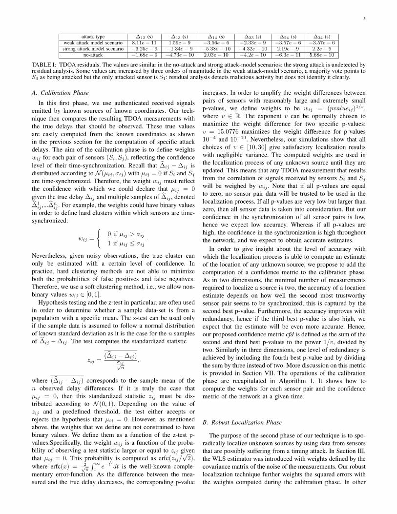
In both scenarios, we consider a two-dimensional grid ofside of 20 km with four sensors placed as in Figures 1 and 2.The unknown source emits a signal that propagates to thefour sensors. We suppose that the sensors send their receivedsignal samples to a control center that processes them. Theresulting TDOA measurements are given as input to the WLS

4

-10 -8 -6 -4 -2 0 2 4 6 8

X position (km)

-10-8-6-4-20246810

Y p

ositi

on (k

m)

10

sensor1: 2.47e-6ssensor2: 0ssensor3: 0ssensor4: 0ssource (true location)

Fig. 1: Weak-attack model scenario: sensor 1 is delayed by 2.47µs.The red TDOA hyperbolae are shifted by this delay and theresulting source estimate is incorrect by approximately 1 km.

estimator as described in Section III. In this simulation, weset the noise standard deviation to σ = 2.192ns for all TDOAmeasurements, this value is further discussed in Section VII.In the the weak attack-model scenario, the attacker delaysthe time reference of sensor S1 by 2.47µs, which modifiesthe three corresponding hyperbolae, drawn in red in Figure 1.The resulting WLS estimate of the unknown source locationis incorrect by approximately 1 km, thus illustrating thatlocalization from TDOA measurements is highly sensitive totime offsets. As the injected delay increases, the accuracy ofthe estimate decreases. Note that in this scenario, the full set ofmeasurements was considered. Supposing that we consideredonly three linearly independent measurements with respect tosensor S1, then the estimate would be even less accurate as theWLS estimator would have received only wrong measurementsas input. In other words, only the red hyperbolae from Figure 1would be taken into account and none of the black ones.

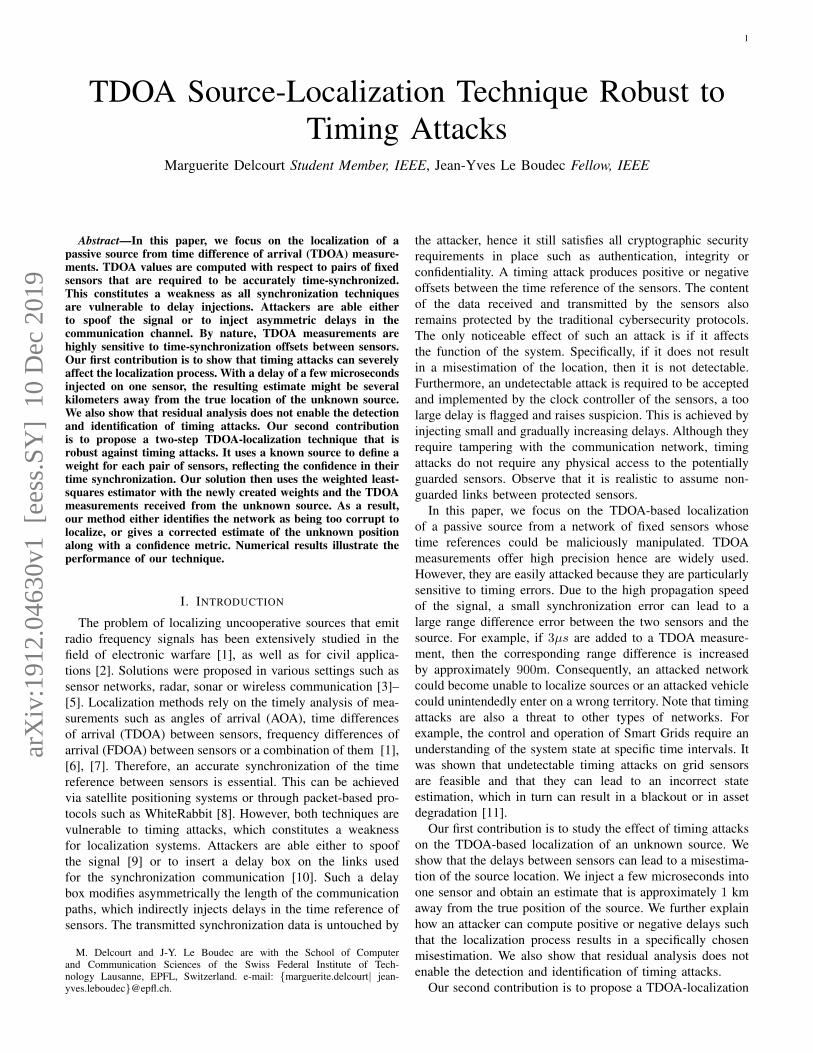
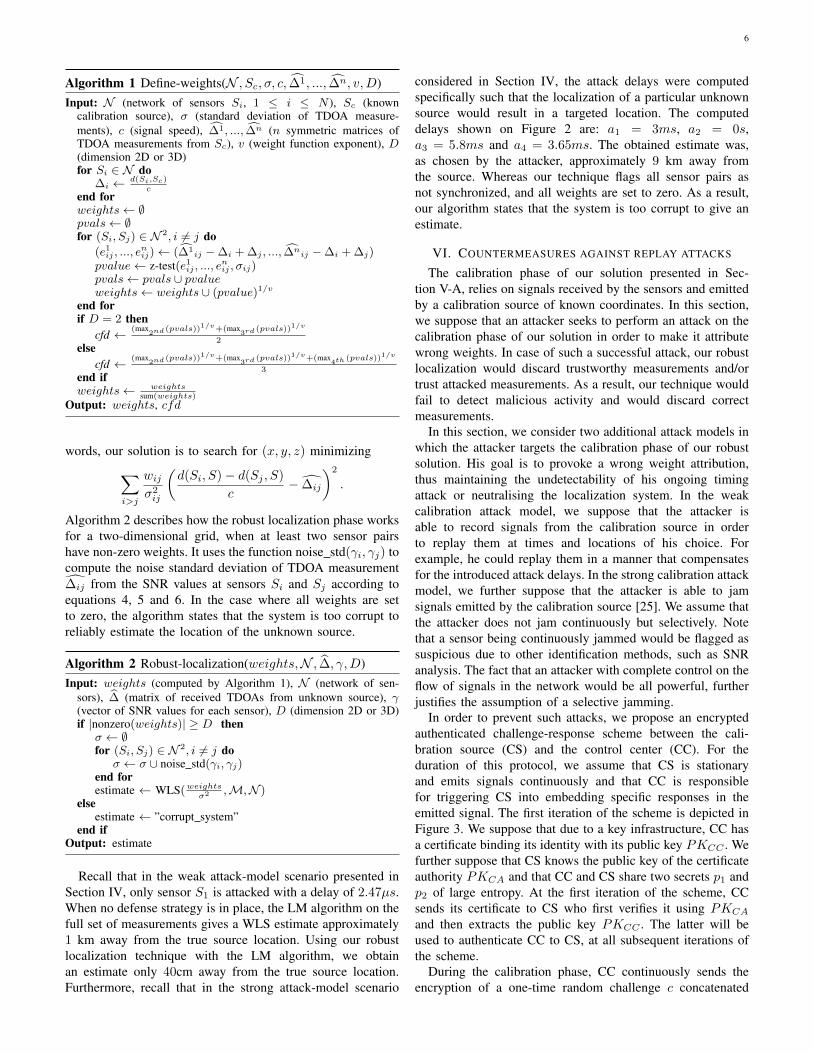
In the strong attack-model scenario, the attacker knows thecoordinates of the sensors and the true coordinates of thesource. With such knowledge, he is able to compute the delaysto be injected such that the estimation process results in aspecific targeted misestimation:• From the source and sensor coordinates, he computes

the true delays of propagation of the signal between thesource and the sensors ∆i = d(Si,S)

c , ∀1 ≤ i ≤ N .• Similarly, he computes the true delays of propagation of

the signal between the targeted misestimation locationand the sensors ∆t

i, ∀1 ≤ i ≤ N .• The attack is simply the difference between the two: the

delay to inject to sensor Si is ai = ∆ti −∆i.

This attack is illustrated in Figure 2, where the delays are com-puted specifically such that all hyperbolae are modified in aplausible manner, intersecting near the targeted misestimationlocation. The resulting estimate is, as chosen by the attacker,almost 9 km away from the true source location.

C. Residual Analysis

Once an estimate Sest is computed from measurementvalues, it is useful to compute and analyze the residuals inorder either to assess the accuracy of the estimator or toattempt to detect and identify bad data in the measurements.

-10 -8 -6 -4 -2 0 2 4 6 8

X position (km)

10

sensor1: 3e-3ssensor2: 0ssensor3: 5.8e-3ssensor4: 3.65e-3ssource (true location)

-10-8-6-4-20246810

Y p

ositi

on (k

m)

Fig. 2: Strong-attack model scenario: delays are strategically com-puted which results in a specific misestimation almost 9 km awayfrom the true source location.

For a pair of sensors (Si, Sj), the corresponding residual iscomputed as follows

d(Si, Sest)− d(Sj , Sest)

c− ∆ij .

The residuals give insight on how well the estimate fits themeasurements. Hence, if all hyperbolae intersect near theestimated location, then the residuals will have small values.However, if the points of intersection of the hyperbolae definea large probable zone of location, then the resulting estimatewill be far from some or all hyperbolae, thus resulting in largeresiduals. Residual values are given in Table I for the no-attackscenario and for the scenarios depicted in Figures 1 and 2 thatcorrespond to the two attack models. Observe that the strongattack-model scenario and the no-attack scenario have similarresiduals of order of magnitude below a nanosecond. This isas expected because, in both cases, the estimate satisfies wellall measurements. Against the strong attack model the residualanalysis fails to detect the presence of malicious activity. In theweak attack-model scenario, Table I shows that three residualshave values by three orders of magnitude larger than theircorresponding values in the no-attack scenario. However, theselarge residuals are not all related to sensor S1. In this case,the residual analysis succeeds in detecting the presence ofmalicious activity in the system but fails to identify it clearly.Overall, residual analysis is misleading for this study as iteither fails to detect the presence of an attack or fails toidentify untrustworthy measurements. Another approach forbuilding resilience against timing attacks is proposed in thefollowing section.

V. CALIBRATION-BASED ROBUST LOCALIZATION

As mentioned above, the analysis of residuals during thelocalization of an unknown source is not sufficient to countertiming attacks. In this section, we present a robust localizationstrategy that works in two phases. The first is a calibrationphase that makes use of a known source to estimate the pair-wise synchronized sensors of the network. The second phaseof our strategy consists in the localization of an unknownsource, given the results of the calibration process. We alsoshow how to compute a confidence metric that gives insighton the accuracy of the estimated location.

5

attack type ∆12 (s) ∆13 (s) ∆14 (s) ∆23 (s) ∆24 (s) ∆34 (s)weak attack model scenario 8.11e− 11 1.59e− 9 −3.56e− 6 −2.33e− 9 −3.57e− 6 −3.57e− 6strong attack model scenario −3.25e− 9 −1.34e− 9 −5.38e− 10 −4.32e− 10 2.19e− 9 2.2e− 9

no-attack −1.68e− 9 −4.73e− 10 2.03e− 10 −4.2e− 10 −6.3e− 11 5.68e− 10

TABLE I: TDOA residuals. The values are similar in the no-attack and strong attack-model scenarios: the strong attack is undetected byresidual analysis. Some values are increased by three orders of magnitude in the weak attack-model scenario, a majority vote points toS4 as being attacked but the only attacked sensor is S1: residual analysis detects malicious activity but does not identify it clearly.

A. Calibration Phase

In this first phase, we use authenticated received signalsemitted by known sources of known coordinates. Our tech-nique then compares the resulting TDOA measurements withthe true delays that should be observed. These true valuesare easily computed from the known coordinates as shownin the previous section for the computation of specific attackdelays. The aim of the calibration phase is to define weightswij for each pair of sensors (Si, Sj), reflecting the confidencelevel of their time-synchronization. Recall that ∆ij − ∆ij isdistributed according to N (µij , σij) with µij = 0 if Si and Sjare time-synchronized. Therefore, the weight wij must reflectthe confidence with which we could declare that µij = 0

given the true delay ∆ij and multiple samples of ∆ij , denoted∆1ij ,...∆

nij . For example, the weights could have binary values

in order to define hard clusters within which sensors are time-synchronized:

wij =

{0 if µij > σij

1 if µij ≤ σij.

Nevertheless, given noisy observations, the true cluster canonly be estimated with a certain level of confidence. Inpractice, hard clustering methods are not able to minimizeboth the probabilities of false positives and false negatives.Therefore, we use a soft clustering method, i.e., we allow non-binary values wij ∈ [0, 1].

Hypothesis testing and the z-test in particular, are often usedin order to determine whether a sample data-set is from apopulation with a specific mean. The z-test can be used onlyif the sample data is assumed to follow a normal distributionof known standard deviation as it is the case for the n samplesof ∆ij −∆ij . The test computes the standardized statistic

zij =(∆ij −∆ij)

σij√n

,

where (∆ij −∆ij) corresponds to the sample mean of then observed delay differences. If it is truly the case thatµij = 0, then this standardized statistic zij must be dis-tributed according to N (0, 1). Depending on the value ofzij and a predefined threshold, the test either accepts orrejects the hypothesis that µij = 0. However, as mentionedabove, the weights that we define are not constrained to havebinary values. We define them as a function of the z-test p-values.Specifically, the weight wij is a function of the proba-bility of observing a test statistic larger or equal to zij giventhat µij = 0. This probability is computed as erfc(zij/

√2),

where erfc(x) = 2√π

∫∞xe−t

2

dt is the well-known comple-mentary error-function. As the difference between the mea-sured and the true delay decreases, the corresponding p-value

increases. In order to amplify the weight differences betweenpairs of sensors with reasonably large and extremely smallp-values, we define weights to be wij = (pvalueij)

1/v ,where v ∈ R. The exponent v can be optimally chosen tomaximize the weight difference for two specific p-values:v = 15.0776 maximizes the weight difference for p-values10−4 and 10−10. Nevertheless, our simulations show that allchoices of v ∈ [10, 30] give satisfactory localization resultswith negligible variance. The computed weights are used inthe localization process of any unknown source until they areupdated. This means that any TDOA measurement that resultsfrom the correlation of signals received by sensors Si and Sjwill be weighed by wij . Note that if all p-values are equalto zero, no sensor pair data will be trusted to be used in thelocalization process. If all p-values are very low but larger thanzero, then all sensor data is taken into consideration. But ourconfidence in the synchronization of all sensor pairs is low,hence we expect low accuracy. Whereas if all p-values arehigh, the confidence in the synchronization is high throughoutthe network, and we expect to obtain accurate estimates.

In order to give insight about the level of accuracy withwhich the localization process is able to compute an estimateof the location of any unknown source, we propose to add thecomputation of a confidence metric to the calibration phase.As in two dimensions, the minimal number of measurementsrequired to localize a source is two, the accuracy of a locationestimate depends on how well the second most trustworthysensor pair seems to be synchronized; this is captured by thesecond best p-value. Furthermore, the accuracy improves withredundancy, hence if the third best p-value is also high, weexpect that the estimate will be even more accurate. Hence,our proposed confidence metric cfd is defined as the sum of thesecond and third best p-values to the power 1/v, divided bytwo. Similarly in three dimensions, one level of redundancy isachieved by including the fourth best p-value and by dividingthe sum by three instead of two. More discussion on this metricis provided in Section VII. The operations of the calibrationphase are recapitulated in Algorithm 1. It shows how tocompute the weights for each sensor pair and the confidencemetric of the network at a given time.

B. Robust-Localization Phase

The purpose of the second phase of our technique is to spo-radically localize unknown sources by using data from sensorsthat are possibly suffering from a timing attack. In Section III,the WLS estimator was introduced with weights defined by thecovariance matrix of the noise of the measurements. Our robustlocalization technique further weights the squared errors withthe weights computed during the calibration phase. In other

6

Algorithm 1 Define-weights(N , Sc, σ, c, ∆1, ..., ∆n, v,D)Input: N (network of sensors Si, 1 ≤ i ≤ N ), Sc (known

calibration source), σ (standard deviation of TDOA measure-ments), c (signal speed), ∆1, ..., ∆n (n symmetric matrices ofTDOA measurements from Sc), v (weight function exponent), D(dimension 2D or 3D)for Si ∈ N do

∆i ← d(Si,Sc)c

end forweights← ∅pvals← ∅for (Si, Sj) ∈ N 2, i 6= j do

(e1ij , ..., enij)← (∆1

ij −∆i + ∆j , ..., ∆nij −∆i + ∆j)

pvalue← z-test(e1ij , ..., enij , σij)

pvals← pvals ∪ pvalueweights← weights ∪ (pvalue)1/v

end forif D = 2 then

cfd ← (max2nd (pvals))1/v+(max

3rd(pvals))1/v

2else

cfd ← (max2nd (pvals))1/v+(max

3rd(pvals))1/v+(max

4th(pvals))1/v

3end ifweights← weights

sum(weights)

Output: weights, cfd

words, our solution is to search for (x, y, z) minimizing∑i>j

wijσ2ij

(d(Si, S)− d(Sj , S)

c− ∆ij

)2

.

Algorithm 2 describes how the robust localization phase worksfor a two-dimensional grid, when at least two sensor pairshave non-zero weights. It uses the function noise std(γi, γj) tocompute the noise standard deviation of TDOA measurement∆ij from the SNR values at sensors Si and Sj according toequations 4, 5 and 6. In the case where all weights are setto zero, the algorithm states that the system is too corrupt toreliably estimate the location of the unknown source.

Algorithm 2 Robust-localization(weights,N , ∆, γ,D)Input: weights (computed by Algorithm 1), N (network of sen-

sors), ∆ (matrix of received TDOAs from unknown source), γ(vector of SNR values for each sensor), D (dimension 2D or 3D)if |nonzero(weights)| ≥ D then

σ ← ∅for (Si, Sj) ∈ N 2, i 6= j do

σ ← σ ∪ noise std(γi, γj)end forestimate ← WLS(weights

σ2 ,M,N )else

estimate ← ”corrupt system”end if

Output: estimate

Recall that in the weak attack-model scenario presented inSection IV, only sensor S1 is attacked with a delay of 2.47µs.When no defense strategy is in place, the LM algorithm on thefull set of measurements gives a WLS estimate approximately1 km away from the true source location. Using our robustlocalization technique with the LM algorithm, we obtainan estimate only 40cm away from the true source location.Furthermore, recall that in the strong attack-model scenario

considered in Section IV, the attack delays were computedspecifically such that the localization of a particular unknownsource would result in a targeted location. The computeddelays shown on Figure 2 are: a1 = 3ms, a2 = 0s,a3 = 5.8ms and a4 = 3.65ms. The obtained estimate was,as chosen by the attacker, approximately 9 km away fromthe source. Whereas our technique flags all sensor pairs asnot synchronized, and all weights are set to zero. As a result,our algorithm states that the system is too corrupt to give anestimate.

VI. COUNTERMEASURES AGAINST REPLAY ATTACKS

The calibration phase of our solution presented in Sec-tion V-A, relies on signals received by the sensors and emittedby a calibration source of known coordinates. In this section,we suppose that an attacker seeks to perform an attack on thecalibration phase of our solution in order to make it attributewrong weights. In case of such a successful attack, our robustlocalization would discard trustworthy measurements and/ortrust attacked measurements. As a result, our technique wouldfail to detect malicious activity and would discard correctmeasurements.

In this section, we consider two additional attack models inwhich the attacker targets the calibration phase of our robustsolution. His goal is to provoke a wrong weight attribution,thus maintaining the undetectability of his ongoing timingattack or neutralising the localization system. In the weakcalibration attack model, we suppose that the attacker isable to record signals from the calibration source in orderto replay them at times and locations of his choice. Forexample, he could replay them in a manner that compensatesfor the introduced attack delays. In the strong calibration attackmodel, we further suppose that the attacker is able to jamsignals emitted by the calibration source [25]. We assume thatthe attacker does not jam continuously but selectively. Notethat a sensor being continuously jammed would be flagged assuspicious due to other identification methods, such as SNRanalysis. The fact that an attacker with complete control on theflow of signals in the network would be all powerful, furtherjustifies the assumption of a selective jamming.

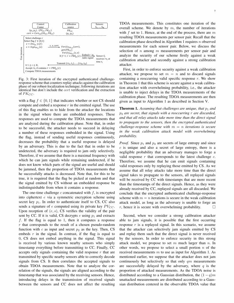
In order to prevent such attacks, we propose an encryptedauthenticated challenge-response scheme between the cali-bration source (CS) and the control center (CC). For theduration of this protocol, we assume that CS is stationaryand emits signals continuously and that CC is responsiblefor triggering CS into embedding specific responses in theemitted signal. The first iteration of the scheme is depicted inFigure 3. We suppose that due to a key infrastructure, CC hasa certificate binding its identity with its public key PKCC . Wefurther suppose that CS knows the public key of the certificateauthority PKCA and that CC and CS share two secrets p1 andp2 of large entropy. At the first iteration of the scheme, CCsends its certificate to CS who first verifies it using PKCA

and then extracts the public key PKCC . The latter will beused to authenticate CC to CS, at all subsequent iterations ofthe scheme.

During the calibration phase, CC continuously sends theencryption of a one-time random challenge c concatenated

7

Control Center

Calibration source

SensorsS", … , S%

&", &' , ()**, (+**,-./ = 1-./*2 34**, (+**

(+*2(&", &')

Select challenge ,Select flag 7 ∈ {0,1}- = =>,?@ (,|7)B = CDE>FGHH(-)

B, -, ,-./ )-.D7IFJKL ,-./ ,E-/((+**))-.D7IFJKK B, -

If 7=1: . = (MN?O(,)Embed . in radio signal

Sensor CPreceives .BP at time /PTransmit (.B", /"), … , (.BQ, /Q)

∀ 1 ≤ D ≤ T,Accept .BP if contains . = (MN?O(,)Compute TDOA measurements

Firs

tite

ratio

n

Fig. 3: First iteration of the encrypted authenticated challenge-response scheme that counters replay attacks against the calibrationphase of our robust-localization technique; following iterations areidentical but don’t include the cert verification and the extractionof PKCC .

with a flag f ∈ {0, 1} that indicates whether or not CS shouldcompute and embed a response r in the emitted signal. The useof this flag enables us to hide from the attacker the locationsin the signal where there are embedded responses. Theseresponses are used to compute the TDOA measurements thatare analyzed during the calibration phase. Note that, in orderto be successful, the attacker needs to succeed in delayinga number of these responses embedded in the signal. Usingthe flag, instead of sending useful responses continuously,decreases the probability that a useful response is delayedby an adversary. This is due to the fact that in order to beundetected, the adversary is required to jam only selectively.Therefore, if we assume that there is a maximal frequency withwhich he can jam signals while remaining undetected, if hedoes not know which parts of the signal are useful and shouldbe jammed, then the proportion of TDOA measurements thathe successfully attacks is decreased. Note that, for this to betrue, it is required that the flag be picked at random and thatthe signal emitted by CS without an embedded response beindistinguishable from when it contains a response.

The one-time challenge c concatenated with f , is encryptedinto ciphertext e via a symmetric encryption scheme usingsecret key p1. In order to authenticate itself to CS, CC alsosends a signature of e computed using its private key PVCC .Upon reception of (e, s), CS verifies the validity of the pairsent by CC. If it is valid, CS decrypts e using p1 and extractsf . If the flag is equal to 1, then it computes a responser that corresponds to the result of a chosen pseudo-randomfunction with c as input and secret p2 as the key. Then, CSembeds r in the signal. In contrast, if the flag is equal to0, CS does not embed anything in the signal. This signalis received by various known nearby sensors who simplytimestamp everything before transmitting to CC. Finally, CCaccepts only signals containing the valid response r that aretransmitted by specific nearby sensors able to correctly decodesignals from CS. It then correlates the accepted signals toobtain TDOA measurements. Note that to analyze the cor-relation of the signals, the signals are aligned according to thetimestamp that was associated by the receiving sensors. Hence,introducing delays in the transmission of received signalsbetween the sensors and CC does not affect the resulting

TDOA measurements. This constitutes one iteration of theoverall scheme. We denote by m, the number of iterationswith f set to 1. Hence, at the end of the process, there are mresulting TDOA measurements per sensor pair. Recall that thecalibration phase described in Algorithm 1 requires n observedmeasurements for each sensor pair. Below, we discuss theselection of n among m measurements per sensor pair andanalyze the security of our scheme firstly against a weakcalibration attacker and secondly against a strong calibrationattacker.

First, in order to enforce security against a weak calibrationattacker, we propose to set m = n and to discard signalscontaining a reoccurring valid specific response r. We showin Theorem 1 that this scheme is secure against a weak calibra-tion attacker with overwhelming probability, i.e., the attackeris unable to inject delays in the TDOA measurements of thecalibration phase. The resulting TDOA measurements are thengiven as input to Algorithm 1 as described in Section V.

Theorem 1. Assuming that challenges are unique, that p1 andp2 are secret, that signals with a reoccurring r are discarded,and that all relay attacks take more time than the direct signalto propagate to the sensors, then the encrypted authenticatedchallenge-response scheme with m = n iterations is securein the weak calibration attack model with overwhelmingprobability.

Proof. Since p1 and p2 are secrets of large entropy and sincec is unique and also a secret of large entropy, there is anegligible probability that an adversary manages to forge avalid response r that corresponds to the latest challenge c.Therefore, we assume that he can emit signals containingvalid responses only by replaying those emitted by CS. As weassume that all relay attacks take more time than the directsignal takes to propagate to the sensors, all replayed signalswill be received by CC with timestamps that are more recentthan the timestamps of the direct signals. Hence, as they werealready received by CC, replayed signals are all discarded. Weconclude that the encrypted authenticated challenge-responsescheme with m = n iterations is secure in the weak calibrationattack model, as long as the adversary is unable to forge anr, hence it is secure with overwhelming probability.

Second, when we consider a strong calibration attackerable to jam signals, it is possible that the first occurringresponse r is a replayed signal. In this scenario, we assumethat the attacker can selectively jam signals emitted by CSand replay them such that the direct signal is never receivedby the sensors. In order to enforce security in this strongattack model, we propose to set m much larger than n. Inother words, we propose to select a small portion n of thereceived measurements m to use as input for Algorithm 1. Asmentioned earlier, we suppose that the attacker does not jamcontinuously but selectively so that only qm measurementsare successfully delayed by the adversary, where q is theproportion of attacked measurements. As the TDOA noise isdistributed according to a Gaussian distribution, the (1− q)munattacked measurements are distributed according to a Gaus-sian distribution centered in the observable TDOA value that

8

depends on the coordinates of the sensors, the coordinatesof CS and the possible time-synchronization offset betweenthe sensors. In contrast, the qm attacked measurements areexpected to be distributed according to another Gaussiandistribution centered around a value that depends on the delaydifference with which the signal is replayed to the differentsensors.

Our strategy is to analyze the distribution of the m observedmeasurements in order to extract the center of the tallestGaussian distribution and to select the n measurements that arenearest to it. More specifically, we use a binning algorithm onall the received measurements; the algorithm returns b bins ofuniform width covering the range of the m measurements. Thisreveals the shape of the sample distribution. We then extractthe bin of highest density and iteratively extract its surroundingbins, until the sub-sampled dataset is of cardinality at leastn. Then, we estimate the probability density function of theselected data and search for its peak value. As a result, weobtain an estimate of the center of the tallest underlyingGaussian distribution, in other words, of the TDOA value thatshould be observed. Finally, we select the n measurementsthat are nearest to the newly found estimate. Observe thatthis technique works in favour of the system only when thereare fewer attacked than unattacked measurements during thecalibration phase. Otherwise, the tallest Gaussian distributionwould correspond to the underlying distribution of the attackedmeasurements. These selected measurements can then be givenas input to Algorithm 1 as described in Section V. We showthe following claim through numerical analysis in Appendix.

Claim 1. As long as the proportion q of attacked measure-ments is lower or equal to 0.45, our strategy is secure againsta strong calibration attacker.

VII. PERFORMANCE EVALUATION

In this section, we evaluate the performance of our solutionpresented in Section V by considering various attack scenarios.We show through Matlab simulations that our solution isrobust to timing attacks and that the confidence metric isreliable. We start by defining the testing environment in twodimensions. We then consider a three-dimensional simulation.

A. Two-Dimensional Testing Environment

We consider a two-dimensional grid of side of 20 km onwhich we place four sensors, as illustrated in figures 1 and 2.We assume that at the time instant of the analysis, the unknownsource is located at coordinates [3333.3,−889.1111] and theknown calibration source at [0,−4000] all in meters, withrespect to the center of the grid. In Section VII-D, we showa three-dimensional simulation on the same grid, to which weadd altitude coordinates. In our simulations, we assume thatthe TDOA noise is i.i.d with a standard deviation of 2.192nsfor all measurements. We computed this standard deviationfrom Eqs. 4, 5, 6 with the following parameters:• the integration window of the signal Tint = 60 ms,• the bandwidth of the signal W = 1 MHz,• the center of frequency f0 = 30′000 Hz,

• the SNR γi = 3 dB ∀Si.For the calibration phase, we created simulated TDOA mea-surements ∆ij from the known calibration source for all sensorpairs (Si, Sj) with the following procedure:• we use the coordinates to compute the true time ∆i taken

by the signal to propagate from the calibration source tosensor Si for both sensors,

• we compute the true TDOA ∆ij = ∆i −∆j ,• depending on the attack scenario, we add delays

∆′ij = ∆ij + ai − aj ,• we add Gaussian noise ∆ij = ∆′ij + eij

with eij ∈ N (0, 2.192e− 9),• we repeat this n = 15 times in order to have 15

measurements for each pair of sensors.Our calibration procedure defined by Algorithm 1 then usesthe simulated measurements in the following way:

1) We compute the observed error eij = ∆ij − ∆ij foreach measurement, using the known coordinates of thecalibration source.

2) For each pair of sensors, we compute the p-value result-ing from the z-test with the 15 observed errors eij .

3) We compute the weights w by exponentiating all p-values to 1/v with v = 15.0776 and normalizing them.

4) We compute the confidence metric as the sum of thesecond and third largest weights before normalization,divided by two.

Recall that the exponent value was chosen to maximise theweight difference between p-values 10−4 and 10−10 and thatwe experimentally observed that all choices of v ∈ [10, 30]give satisfactory results with low variance between them.

For each pair of sensors such that the corresponding weightis non-zero, we create a simulated TDOA measurement ∆ij

from the unknown source to localize:• we use the coordinates to compute the true time ∆i taken

by the signal to propagate from the unknown source tosensor Si for both sensors,

• we compute the true TDOA ∆ij = ∆i −∆j ,• depending on the attack scenario, we add delays

∆′ij = ∆ij + ai − aj ,• we add Gaussian noise ∆ij = ∆′ij + eij

with eij ∈ N (0, 2.192e− 9).We implement the robust localization with the simulatedmeasurements as in Algorithm 2:

1) We compute a geometrical estimate of the source loca-tion (xg, yg) as explained below.

2) We use the Matlab LM algorithm as a WLS estimatoron all ∆ij with weights wij computed at step (3).The initial step size is by default 0.01 and the initialsolution is (xg, yg). We obtain the estimated robustsource coordinates (x, y).

In all simulations, we analyze the confidence metric and thedistance between our estimate and the true source coordinates.

Recall that the WLS estimator we use is the LM algorithm.It is a gradient descent algorithm that requires an initialsolution and step size that are updated iteratively. When thegradient is small, the step size is chosen small so that we can

9

move gradually closer to the minima without missing it; in thiscase the algorithm is similar to the Gauss-Newton method. Incontrast, when the gradient is large, the step size is chosenlarge and the algorithm behaves similarly to the steepestdescent method. The initial solution we use is a geometricalestimate computed as the coordinate-wise weighted medianof intersection points of all hyperbolae. The weight of bothcoordinates of an intersection point corresponds to the smallestweight among the weights of the corresponding TDOAs.

B. Performance in Attack Scenarios

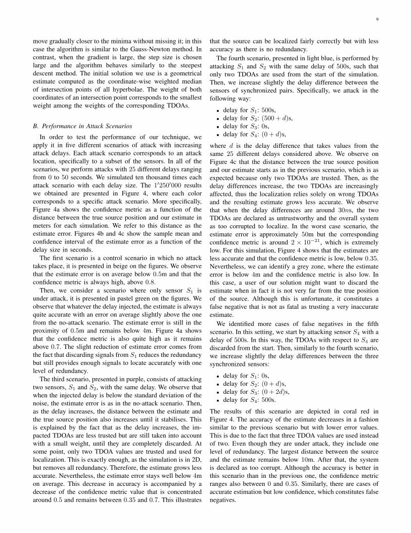
In order to test the performance of our technique, weapply it in five different scenarios of attack with increasingattack delays. Each attack scenario corresponds to an attacklocation, specifically to a subset of the sensors. In all of thescenarios, we perform attacks with 25 different delays rangingfrom 0 to 50 seconds. We simulated ten thousand times eachattack scenario with each delay size. The 1′250′000 resultswe obtained are presented in Figure 4, where each colorcorresponds to a specific attack scenario. More specifically,Figure 4a shows the confidence metric as a function of thedistance between the true source position and our estimate inmeters for each simulation. We refer to this distance as theestimate error. Figures 4b and 4c show the sample mean andconfidence interval of the estimate error as a function of thedelay size in seconds.

The first scenario is a control scenario in which no attacktakes place, it is presented in beige on the figures. We observethat the estimate error is on average below 0.5m and that theconfidence metric is always high, above 0.8.

Then, we consider a scenario where only sensor S1 isunder attack, it is presented in pastel green on the figures. Weobserve that whatever the delay injected, the estimate is alwaysquite accurate with an error on average slightly above the onefrom the no-attack scenario. The estimate error is still in theproximity of 0.5m and remains below 4m. Figure 4a showsthat the confidence metric is also quite high as it remainsabove 0.7. The slight reduction of estimate error comes fromthe fact that discarding signals from S1 reduces the redundancybut still provides enough signals to locate accurately with onelevel of redundancy.

The third scenario, presented in purple, consists of attackingtwo sensors, S1 and S2, with the same delay. We observe thatwhen the injected delay is below the standard deviation of thenoise, the estimate error is as in the no-attack scenario. Then,as the delay increases, the distance between the estimate andthe true source position also increases until it stabilises. Thisis explained by the fact that as the delay increases, the im-pacted TDOAs are less trusted but are still taken into accountwith a small weight, until they are completely discarded. Atsome point, only two TDOA values are trusted and used forlocalization. This is exactly enough, as the simulation is in 2D,but removes all redundancy. Therefore, the estimate grows lessaccurate. Nevertheless, the estimate error stays well below 4mon average. This decrease in accuracy is accompanied by adecrease of the confidence metric value that is concentratedaround 0.5 and remains between 0.35 and 0.7. This illustrates

that the source can be localized fairly correctly but with lessaccuracy as there is no redundancy.

The fourth scenario, presented in light blue, is performed byattacking S1 and S2 with the same delay of 500s, such thatonly two TDOAs are used from the start of the simulation.Then, we increase slightly the delay difference between thesensors of synchronized pairs. Specifically, we attack in thefollowing way:

• delay for S1: 500s,• delay for S2: (500 + d)s,• delay for S3: 0s,• delay for S4: (0 + d)s,

where d is the delay difference that takes values from thesame 25 different delays considered above. We observe onFigure 4c that the distance between the true source positionand our estimate starts as in the previous scenario, which is asexpected because only two TDOAs are trusted. Then, as thedelay differences increase, the two TDOAs are increasinglyaffected, thus the localization relies solely on wrong TDOAsand the resulting estimate grows less accurate. We observethat when the delay differences are around 30ns, the twoTDOAs are declared as untrustworthy and the overall systemas too corrupted to localize. In the worst case scenario, theestimate error is approximately 50m but the correspondingconfidence metric is around 2 × 10−21, which is extremelylow. For this simulation, Figure 4 shows that the estimates areless accurate and that the confidence metric is low, below 0.35.Nevertheless, we can identify a grey zone, where the estimateerror is below 4m and the confidence metric is also low. Inthis case, a user of our solution might want to discard theestimate when in fact it is not very far from the true positionof the source. Although this is unfortunate, it constitutes afalse negative that is not as fatal as trusting a very inaccurateestimate.

We identified more cases of false negatives in the fifthscenario. In this setting, we start by attacking sensor S4 with adelay of 500s. In this way, the TDOAs with respect to S4 arediscarded from the start. Then, similarly to the fourth scenario,we increase slightly the delay differences between the threesynchronized sensors:

• delay for S1: 0s,• delay for S2: (0 + d)s,• delay for S3: (0 + 2d)s,• delay for S4: 500s.

The results of this scenario are depicted in coral red inFigure 4. The accuracy of the estimate decreases in a fashionsimilar to the previous scenario but with lower error values.This is due to the fact that three TDOA values are used insteadof two. Even though they are under attack, they include onelevel of redundancy. The largest distance between the sourceand the estimate remains below 10m. After that, the systemis declared as too corrupt. Although the accuracy is better inthis scenario than in the previous one, the confidence metricranges also between 0 and 0.35. Similarly, there are cases ofaccurate estimation but low confidence, which constitutes falsenegatives.

10

Fig. 4: Results from five different timing attack scenarios each with 25 different delays, each simulated 10′000 times: (a) confidencemetric as a function of the distance between the true source position and the estimate provided by our robust solution, we observe that themetric is related to the accuracy and shows if there is redundancy in the measurements. There are some false-negative cases but no falsepositives. (b) the mean and confidence interval of the estimate error for each attack delay for three different scenarios. (c) the mean andconfidence interval of the estimate error for each attack delay for two other scenarios: when the system is too corrupt, it stops localizing.

In summary, our method gives an estimate which is alwaysquite accurate, considering the fact that blindly trusting allTDOAs would lead to errors of many kilometers. Whenthe system is too corrupt, it declares that the confidencelevel is too low to localize. We showed that the confidencemetric gives useful insight on the accuracy of the estimate,although it can lead to some false-negative cases. We have notfound any corner cases of false positives, in other words, oursolution never trusts a highly inaccurate solution. If we wereto recommend a course of action depending on the confidencemetric, it would be the following:• confidence metric ∈ [0.75, 1]: trust the estimate to be as

accurate as it can be because it includes at least one levelof redundancy,

• confidence metric ∈ [0.3, 0.75]: probably computed withno redundancy, trust the estimate to be fairly correct butslightly less accurate,

• confidence metric ∈ [0, 0.3]: the true source is in aprobable zone around the estimate, this result is not veryaccurate and trusting it depends on the application,

• algorithm 2 output is ”corrupt system”: the attacks aretoo important to define even a probable zone of location.

C. Trajectory Simulations

Next, we simulate the localization of an unknown source atnine different time instants and compare the true trajectory, thetrajectory estimated with our robust solution, and the trajectorynaively estimated by trusting all measurements. The naiveestimates are found by the WLS estimator with all weightsset to 1. This section shows that our solution substantiallyimproves the accuracy of the estimates when compared withthe accuracy of the naive estimates obtained by ignoring thepresence of timing attacks. We do so in three different attackscenarios, one for each confidence metric interval identifiedabove.

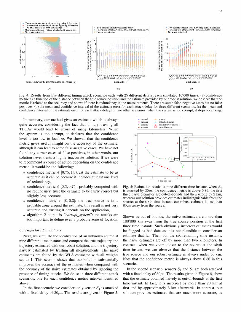
In the first scenario we consider, only sensor S4 is attackedwith a fixed delay of 30µs. The results are given in Figure 5.

sensor1sensor2sensor3sensor4

sourcerobust estimatesnon-robust estimates

-10 -8 -6 -4 -2X position (km)

-10

-5

0

5

10

Y p

ositi

on (k

m)

OB

OB out-of-bounds

-2081.4

-2081.2

-2081

-2080.8

-2080.6

-2080.4

2621 2621.2 2621.4 2621.6 2621.8X position (m)

Y p

ositi

on (m

)

Fig. 5: Estimation results at nine different time instants when S4is attacked by 30µs, the confidence metric is above 0.86: the firstthree naive estimates are out-of-bounds and then wrong by 2 km,whereas our solution provides estimates indistinguishable from thesource; at the sixth time instant, our robust estimate is less than60cm away from the source.

Shown as out-of-bounds, the naive estimates are more than100′000 km away from the true source position at the firstthree time instants. Such obviously incorrect estimates wouldbe flagged as bad data as it is not plausible to consider anestimate that far. Then, for the six remaining time instants,the naive estimates are off by more than two kilometers. Incontrast, when we zoom closer to the source at the sixthtime instant, we can observe that the distance between thetrue source and our robust estimate is always under 60 cm.Note that the confidence metric is always above 0.86 in thisscenario.

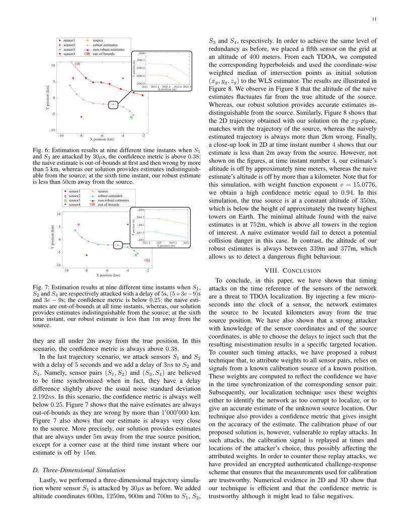
In the second scenario, sensors S1 and S3 are both attackedwith a fixed delay of 30µs. The results given in Figure 6, showthat the estimate obtained naively is out-of-bounds at the firsttime instant. In fact, it is incorrect by more than 20 km atfirst and by approximately 5 km afterwards. In contrast, oursolution provides estimates that are much more accurate, as

11

-10 -8 -6 -4 -2X position (km)

-10

-5

0

5

10

Y p

ositi

on (k

m)

sensor1sensor2sensor3sensor4

sourcerobust estimatesnon-robust estimates

OB out-of-bounds

OB

2621 2621.2 2621.4 2621.6 2621.8

-2080

-2080.8

-2080.6

-2080.4

-2080.2

X position (m)

Y p

ositi

on (m

)

Fig. 6: Estimation results at nine different time instants when S1and S3 are attacked by 30µs, the confidence metric is above 0.38:the naive estimate is out-of-bounds at first and then wrong by morethan 5 km, whereas our solution provides estimates indistinguish-able from the source; at the sixth time instant, our robust estimateis less than 50cm away from the source.

-10 -8 -6 -4 -2X position (km)

-10

-5

0

5

10

Y p

ositi

on (k

m)

sensor1sensor2sensor3

sourcerobust estimatesnon-robust estimates

OB out-of-bounds

OB

sensor4

2621.5 2622 2622.5 2623-2082

-2081.5

-2081

-2080.5

-2080

X position (m)

Y p

ositi

on (m

)

Fig. 7: Estimation results at nine different time instants when S1,S2 and S4 are respectively attacked with a delay of 5s, (5+3e−9)sand 3e − 9s; the confidence metric is below 0.25: the naive esti-mates are out-of-bounds at all time instants, whereas, our solutionprovides estimates indistinguishable from the source; at the sixthtime instant, our robust estimate is less than 1m away from thesource.

they are all under 2m away from the true position. In thisscenario, the confidence metric is always above 0.38.

In the last trajectory scenario, we attack sensors S1 and S2

with a delay of 5 seconds and we add a delay of 3ns to S2 andS4. Namely, sensor pairs (S1, S2) and (S3, S4) are believedto be time synchronized when in fact, they have a delaydifference slightly above the usual noise standard deviation2.192ns. In this scenario, the confidence metric is always wellbelow 0.25. Figure 7 shows that the naive estimates are alwaysout-of-bounds as they are wrong by more than 1′000′000 km.Figure 7 also shows that our estimate is always very closeto the source. More precisely, our solution provides estimatesthat are always under 5m away from the true source position,except for a corner case at the third time instant where ourestimate is off by 15m.

D. Three-Dimensional Simulation

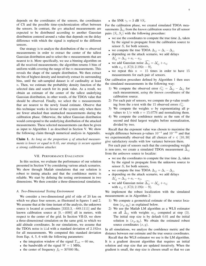
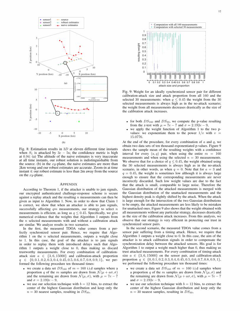
Lastly, we performed a three-dimensional trajectory simula-tion where sensor S1 is attacked by 30µs as before. We addedaltitude coordinates 600m, 1250m, 900m and 700m to S1, S2,

S3 and S4, respectively. In order to achieve the same level ofredundancy as before, we placed a fifth sensor on the grid atan altitude of 400 meters. From each TDOA, we computedthe corresponding hyperboloids and used the coordinate-wiseweighted median of intersection points as initial solution(xg, yg, zg) to the WLS estimator. The results are illustrated inFigure 8. We observe in Figure 8 that the altitude of the naiveestimates fluctuates far from the true altitude of the source.Whereas, our robust solution provides accurate estimates in-distinguishable from the source. Similarly, Figure 8 shows thatthe 2D trajectory obtained with our solution on the xy-plane,matches with the trajectory of the source, whereas the naivelyestimated trajectory is always more than 2km wrong. Finally,a close-up look in 2D at time instant number 4 shows that ourestimate is less than 2m away from the source. However, notshown on the figures, at time instant number 4, our estimate’saltitude is off by approximately nine meters, whereas the naiveestimate’s altitude is off by more than a kilometer. Note that forthis simulation, with weight function exponent v = 15.0776,we obtain a high confidence metric equal to 0.94. In thissimulation, the true source is at a constant altitude of 350m,which is below the height of approximately the twenty highesttowers on Earth. The minimal altitude found with the naiveestimates is at 752m, which is above all towers in the regionof interest. A naive estimator would fail to detect a potentialcollision danger in this case. In contrast, the altitude of ourrobust estimates is always between 339m and 377m, whichallows us to detect a dangerous flight behaviour.

VIII. CONCLUSION

To conclude, in this paper, we have shown that timingattacks on the time reference of the sensors of the networkare a threat to TDOA localization. By injecting a few micro-seconds into the clock of a sensor, the network estimatesthe source to be located kilometers away from the truesource position. We have also shown that a strong attackerwith knowledge of the sensor coordinates and of the sourcecoordinates, is able to choose the delays to inject such that theresulting misestimation results in a specific targeted location.To counter such timing attacks, we have proposed a robusttechnique that, to attribute weights to all sensor pairs, relies onsignals from a known calibration source of a known position.These weights are computed to reflect the confidence we havein the time synchronization of the corresponding sensor pair.Subsequently, our localization technique uses these weightseither to identify the network as too corrupt to localize, or togive an accurate estimate of the unknown source location. Ourtechnique also provides a confidence metric that gives insighton the accuracy of the estimate. The calibration phase of ourproposed solution is, however, vulnerable to replay attacks. Insuch attacks, the calibration signal is replayed at times andlocations of the attacker’s choice, thus possibly affecting theattributed weights. In order to counter these replay attacks, wehave provided an encrypted authenticated challenge-responsescheme that ensures that the measurements used for calibrationare trustworthy. Numerical evidence in 2D and 3D show thatour technique is efficient and that the confidence metric istrustworthy although it might lead to false negatives.

12

sensor1sensor2sensor3sensor4

sourcerobust estimatesnaive estimates

01

1000

1

Z po

sitio

n (m

)

2000

0.5

Y position (m)

0

X position (m)

3000

0-0.5-1 -1

(a)

104

104

010

1

10

Z po

sitio

n (k

m) 2

5

Y position (km)0

X position (km)

3

0-5-10 -10

-10 -5 0 5 10X position (km)

-10

-5

0

5

10

Y p

ositi

on (k

m)

(b)

-2000 -1999 -1998X position (m)

-1801

-1800

-1799

-1798

Y p

ositi

on (m

)

Fig. 8: Estimation results in 3D at eleven different time instantswhen S1 is attacked by 3e − 5s; the confidence metric is highat 0.94: (a) The altitude of the naive estimates is very inaccurateat all time instants, our robust solution is indistinguishable fromthe source. (b) in the xy-plane, the naive estimates are more than2km wrong and our robust estimates are accurate. Zoom-in at timeinstant 4: our robust estimate is less than 2m away from the sourceon the xy-plane.

APPENDIX

According to Theorem 1, if the attacker is unable to jam signals,our encrypted authenticated challenge-response scheme is secureagainst a replay attack and the resulting n measurements can then begiven as input to Algorithm 1. Now, in order to show that Claim 1is correct, we show that when an attacker is able to jam signals,successfully affecting qm measurements, our strategy to select nmeasurements is efficient, as long as q ≤ 0.45. Specifically, we givenumerical evidence that the weights that Algorithm 1 outputs fromthe n selected measurements with and without a calibration attackare similar. We analyze results in two scenarios.

In the first, the measured TDOA value comes from a per-fectly synchronized sensor pair. Hence, we require that Algo-rithm 1 on the n selected measurements, outputs a weight closeto 1. In this case, the goal of the attacker is to jam signalsin order to replay them with introduced delays such that Algo-rithm 1 outputs a weight close to 0, thus making us discardtrustworthy measurements. For every combination of calibration-attack size a ∈ {3, 6, 15000} and calibration-attack proportionq ∈ {0, 0.1, 0.2, 0.3, 0.4, 0.45, 0.5, 0.6, 0.7, 0.8, 0.9, 1}, we per-formed the following procedure ten thousand times:

• we create a data set DS160 of m = 160 i.i.d samples where aproportion q of the m samples are drawn from N (µ + aσ, σ)and the remaining are drawn from N (µ, σ), with µ = 7e − 7and σ = 2.192e− 9,

• we use our selection technique with b = 12 bins, to extract thecenter of the highest Gaussian distribution and keep only then = 30 nearest samples, resulting in DS30,

00.10.20.30.40.50.60.70.80.91

resu

lting

wei

ght

attack size and proportion

Computation with all 160 measurementsComputation with selected 30 measurements

0

36

1500

0

0.1

36

1500

0 3 6

1500

0 3 6

1500

0 3 6

1500

0 3 6

1500

0 3 6

1500

0 3 6

1500

0 3 6

1500

0 3 6

1500

0 3 6

1500

0 3 6

1500

0

0.2 0.3 0.4 0.45 0.5 0.6 0.7 0.8 0.9 1

Fig. 9: Weight for an ideally synchronized sensor pair for differentcalibration-attack size and attack proportion from all 160 and theselected 30 measurements: when q ≤ 0.45 the weight from the 30selected measurements is always high as in the no-attack scenario;the weight from all measurements decreases drastically as the size ofthe calibration attack increases.

• for both DS160 and DS30, we compute the p-value resultingfrom the z-test with µ = 7e− 7 and σ = 2.192e− 9,

• we apply the weight function of Algorithm 1 to the two p-values: we exponentiate them to the power 1/v with v =15.0776.

At the end of the procedure, for every combination of a and q, weobtain two data sets of ten thousand exponentiated p-values. Figure 9shows the sample mean of the resulting weights with a confidenceinterval for every (a, q) pair, when using the entire m = 160measurements and when using the selected n = 30 measurements.We observe that for a choice of q ≤ 0.45, the weight obtained usingthe 30 selected measurements is always high as in the no-attackscenario, in other words, as when q = 0. Note that for a = 3 andq = 0.45, the weight is sometimes low although it is always largeenough to ensure that the corresponding measurements are neverincorrectly discarded. Such low weight values are due to the factthat the attack is small, comparable to large noise. Therefore theGaussian distribution of the attacked measurements is merged withthe Gaussian distribution of the unattacked measurements and thehighest density peak is slightly shifted by the attack. When the attackis large enough for the intersection of the two Gaussian distributionsto be empty, the attacked measurements are less likely to be mistakenfor unattacked ones. Figure 9 also shows that the weight obtained withall measurements without any particular strategy, decreases drasticallyas the size of the calibration attack increases. From this analysis, weobserve that our strategy is very efficient in protecting our trust insynchronized sensor pairs.

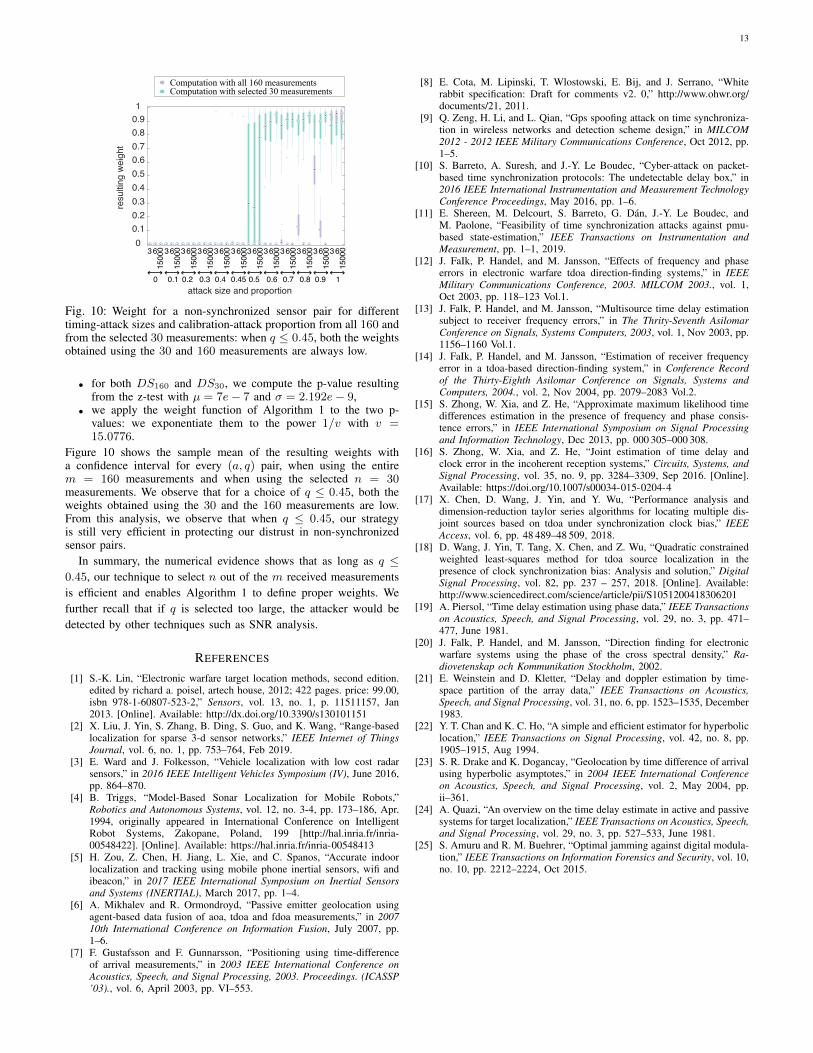
In the second scenario, the measured TDOA value comes from asensor pair suffering from a timing attack. Hence, we require thatAlgorithm 1 outputs a weight close to 0. In this case, the aim of theattacker is to attack calibration signals in order to compensate thesynchronization delay between the attacked sensors. His goal is forAlgorithm 1 to output a weight much higher than 0, thus making ustrust attacked measurements. For every combination of timing-attacksize a ∈ {3, 6, 15000} on the sensor pair, and calibration-attackproportion q ∈ {0, 0.1, 0.2, 0.3, 0.4, 0.45, 0.5, 0.6, 0.7, 0.8, 0.9, 1},we performed the following procedure ten thousand times:

• we create a data set DS160 of m = 160 i.i.d samples wherea proportion q of the m samples are drawn from N (µ, σ) andthe remaining are drawn from N (µ+ aσ, σ), with µ = 7e− 7and σ = 2.192e− 9,

• we use our selection technique with b = 12 bins, to extract thecenter of the highest Gaussian distribution and keep only then = 30 nearest samples, resulting in DS30,

13

Computation with all 160 measurementsComputation with selected 30 measurements

00.10.20.30.40.50.60.70.80.91

resu

lting

wei

ght

attack size and proportion0

36

1500

0

0.1

36

1500

0 3 6

1500

0 3 6

1500

0 3 6

1500

0 3 615

000 3 6

1500

0 3 6

1500

0 3 6

1500

0 3 6

1500

0 3 6

1500

0 3 6

1500

0

0.2 0.3 0.4 0.45 0.5 0.6 0.7 0.8 0.9 1

Fig. 10: Weight for a non-synchronized sensor pair for differenttiming-attack sizes and calibration-attack proportion from all 160 andfrom the selected 30 measurements: when q ≤ 0.45, both the weightsobtained using the 30 and 160 measurements are always low.

• for both DS160 and DS30, we compute the p-value resultingfrom the z-test with µ = 7e− 7 and σ = 2.192e− 9,

• we apply the weight function of Algorithm 1 to the two p-values: we exponentiate them to the power 1/v with v =15.0776.

Figure 10 shows the sample mean of the resulting weights witha confidence interval for every (a, q) pair, when using the entirem = 160 measurements and when using the selected n = 30measurements. We observe that for a choice of q ≤ 0.45, both theweights obtained using the 30 and the 160 measurements are low.From this analysis, we observe that when q ≤ 0.45, our strategyis still very efficient in protecting our distrust in non-synchronizedsensor pairs.

In summary, the numerical evidence shows that as long as q ≤0.45, our technique to select n out of the m received measurementsis efficient and enables Algorithm 1 to define proper weights. Wefurther recall that if q is selected too large, the attacker would bedetected by other techniques such as SNR analysis.

REFERENCES

[1] S.-K. Lin, “Electronic warfare target location methods, second edition.edited by richard a. poisel, artech house, 2012; 422 pages. price: 99.00,isbn 978-1-60807-523-2,” Sensors, vol. 13, no. 1, p. 11511157, Jan2013. [Online]. Available: http://dx.doi.org/10.3390/s130101151

[2] X. Liu, J. Yin, S. Zhang, B. Ding, S. Guo, and K. Wang, “Range-basedlocalization for sparse 3-d sensor networks,” IEEE Internet of ThingsJournal, vol. 6, no. 1, pp. 753–764, Feb 2019.

[3] E. Ward and J. Folkesson, “Vehicle localization with low cost radarsensors,” in 2016 IEEE Intelligent Vehicles Symposium (IV), June 2016,pp. 864–870.

[4] B. Triggs, “Model-Based Sonar Localization for Mobile Robots,”Robotics and Autonomous Systems, vol. 12, no. 3-4, pp. 173–186, Apr.1994, originally appeared in International Conference on IntelligentRobot Systems, Zakopane, Poland, 199 [http://hal.inria.fr/inria-00548422]. [Online]. Available: https://hal.inria.fr/inria-00548413

[5] H. Zou, Z. Chen, H. Jiang, L. Xie, and C. Spanos, “Accurate indoorlocalization and tracking using mobile phone inertial sensors, wifi andibeacon,” in 2017 IEEE International Symposium on Inertial Sensorsand Systems (INERTIAL), March 2017, pp. 1–4.

[6] A. Mikhalev and R. Ormondroyd, “Passive emitter geolocation usingagent-based data fusion of aoa, tdoa and fdoa measurements,” in 200710th International Conference on Information Fusion, July 2007, pp.1–6.

[7] F. Gustafsson and F. Gunnarsson, “Positioning using time-differenceof arrival measurements,” in 2003 IEEE International Conference onAcoustics, Speech, and Signal Processing, 2003. Proceedings. (ICASSP’03)., vol. 6, April 2003, pp. VI–553.

[8] E. Cota, M. Lipinski, T. Wlostowski, E. Bij, and J. Serrano, “Whiterabbit specification: Draft for comments v2. 0,” http://www.ohwr.org/documents/21, 2011.

[9] Q. Zeng, H. Li, and L. Qian, “Gps spoofing attack on time synchroniza-tion in wireless networks and detection scheme design,” in MILCOM2012 - 2012 IEEE Military Communications Conference, Oct 2012, pp.1–5.

[10] S. Barreto, A. Suresh, and J.-Y. Le Boudec, “Cyber-attack on packet-based time synchronization protocols: The undetectable delay box,” in2016 IEEE International Instrumentation and Measurement TechnologyConference Proceedings, May 2016, pp. 1–6.

[11] E. Shereen, M. Delcourt, S. Barreto, G. Dan, J.-Y. Le Boudec, andM. Paolone, “Feasibility of time synchronization attacks against pmu-based state-estimation,” IEEE Transactions on Instrumentation andMeasurement, pp. 1–1, 2019.

[12] J. FaIk, P. Handel, and M. Jansson, “Effects of frequency and phaseerrors in electronic warfare tdoa direction-finding systems,” in IEEEMilitary Communications Conference, 2003. MILCOM 2003., vol. 1,Oct 2003, pp. 118–123 Vol.1.

[13] J. Falk, P. Handel, and M. Jansson, “Multisource time delay estimationsubject to receiver frequency errors,” in The Thrity-Seventh AsilomarConference on Signals, Systems Computers, 2003, vol. 1, Nov 2003, pp.1156–1160 Vol.1.

[14] J. FaIk, P. Handel, and M. Jansson, “Estimation of receiver frequencyerror in a tdoa-based direction-finding system,” in Conference Recordof the Thirty-Eighth Asilomar Conference on Signals, Systems andComputers, 2004., vol. 2, Nov 2004, pp. 2079–2083 Vol.2.

[15] S. Zhong, W. Xia, and Z. He, “Approximate maximum likelihood timedifferences estimation in the presence of frequency and phase consis-tence errors,” in IEEE International Symposium on Signal Processingand Information Technology, Dec 2013, pp. 000 305–000 308.

[16] S. Zhong, W. Xia, and Z. He, “Joint estimation of time delay andclock error in the incoherent reception systems,” Circuits, Systems, andSignal Processing, vol. 35, no. 9, pp. 3284–3309, Sep 2016. [Online].Available: https://doi.org/10.1007/s00034-015-0204-4

[17] X. Chen, D. Wang, J. Yin, and Y. Wu, “Performance analysis anddimension-reduction taylor series algorithms for locating multiple dis-joint sources based on tdoa under synchronization clock bias,” IEEEAccess, vol. 6, pp. 48 489–48 509, 2018.

[18] D. Wang, J. Yin, T. Tang, X. Chen, and Z. Wu, “Quadratic constrainedweighted least-squares method for tdoa source localization in thepresence of clock synchronization bias: Analysis and solution,” DigitalSignal Processing, vol. 82, pp. 237 – 257, 2018. [Online]. Available:http://www.sciencedirect.com/science/article/pii/S1051200418306201

[19] A. Piersol, “Time delay estimation using phase data,” IEEE Transactionson Acoustics, Speech, and Signal Processing, vol. 29, no. 3, pp. 471–477, June 1981.

[20] J. Falk, P. Handel, and M. Jansson, “Direction finding for electronicwarfare systems using the phase of the cross spectral density,” Ra-diovetenskap och Kommunikation Stockholm, 2002.

[21] E. Weinstein and D. Kletter, “Delay and doppler estimation by time-space partition of the array data,” IEEE Transactions on Acoustics,Speech, and Signal Processing, vol. 31, no. 6, pp. 1523–1535, December1983.

[22] Y. T. Chan and K. C. Ho, “A simple and efficient estimator for hyperboliclocation,” IEEE Transactions on Signal Processing, vol. 42, no. 8, pp.1905–1915, Aug 1994.

[23] S. R. Drake and K. Dogancay, “Geolocation by time difference of arrivalusing hyperbolic asymptotes,” in 2004 IEEE International Conferenceon Acoustics, Speech, and Signal Processing, vol. 2, May 2004, pp.ii–361.

[24] A. Quazi, “An overview on the time delay estimate in active and passivesystems for target localization,” IEEE Transactions on Acoustics, Speech,and Signal Processing, vol. 29, no. 3, pp. 527–533, June 1981.

[25] S. Amuru and R. M. Buehrer, “Optimal jamming against digital modula-tion,” IEEE Transactions on Information Forensics and Security, vol. 10,no. 10, pp. 2212–2224, Oct 2015.