TDC 369 / TDC 432 April 2, 2003 Greg Brewster. Topics Math Review Probability –Distributions –Random Variables –Expected Values.

TDC 369 / TDC 432

April 2, 2003

Greg Brewster

Topics

• Math Review

• Probability

– Distributions

– Random Variables

– Expected Values

Math Review

• Simple integrals and differentials

• Sums

• Permutations

• Combinations

• Probability

Math Review: Sums

n

k

nnk

0 2

)1(

n

k

nk

q

qq

0

1

1

1

0 1

1

k

k

qq )1|(| q

)1( q

Math Review:Permutations

• Given N objects, there are N! = N(N-1)…1

different ways to arrange them

• Example: Given 3 balls, colored Red, White and

Blue, there are 3! = 6 ways to order them

– RWB, RBW, BWR, BRW, WBR, WRB

Math Review:Combinations

• The number of ways to select K unique objects

from a set of N objects without replacement is

C(N,K) =

• Example: Given 3 balls, RBW, there are C(3,2) =

3 ways to uniquely choose 2 balls

– RB, RW, BW

)!(!

!

KNK

N

K

N

Probability

• Probability theory is concerned with the

likelihood of observable outcomes (“events”) of

some experiment.

• Let be the set of all outcomes and let E be

some event in , then the probability of E

occurring = Pr[E] is the fraction of times E will

occur if the experiment is repeated infinitely often.

Probability • Example:

– Experiment = tossing a 6-sided die

– Observable outcomes = {1, 2, 3, 4, 5, 6}

– For fair die, • Pr{die = 1} =

• Pr{die = 2} =

• Pr{die = 3} =

• Pr{die = 4} =

• Pr{die = 5} =

• Pr{die = 6} =

6

1

6

1

6

1

6

1

6

1

6

1

Probability Pie

Die=1

Die=2

Die=3Die=4

Die=5

Die=6

Valid Probability Measure• A probability measure, Pr, on an event space

{Ei} must satisfy the following:

– For all Ei , 0 <= Pr[Ei ] <= 1

– Each pair of events, Ei and Ek, are mutually exclusive,

that is,

– All event probabilities sum to 1, that is,

1]Pr[Pr11

kk

kk EE

kiEE ki ,

Probability Mass Function

0

0.2

0.4

0.6

0.8

1

1 2 3 4 5 6

Pr(Die = x)

Mass Function = Histogram

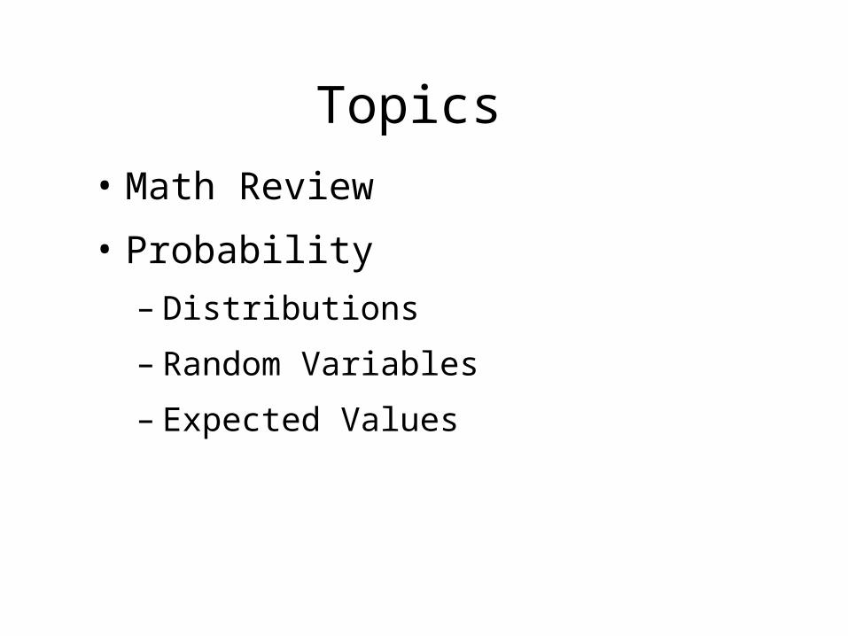
• If you are starting with some repeatable events,

then the Probability Mass function is like a

histogram of outcomes for those events.

• The difference is a histogram indicates how

many times an event happened (out of some

total number of attempts), while a mass

function shows the fraction of time an event

happens (number of times / total attempts).

Dice Roll Histogram1200 attempts

0

50

100

150

200

250

1 2 3 4 5 6

Number of times Die = x

Probability Distribution Function(Cumulative Distribution Function)

0

0.2

0.4

0.6

0.8

1

1 2 3 4 5 6

Pr(Die <= x)

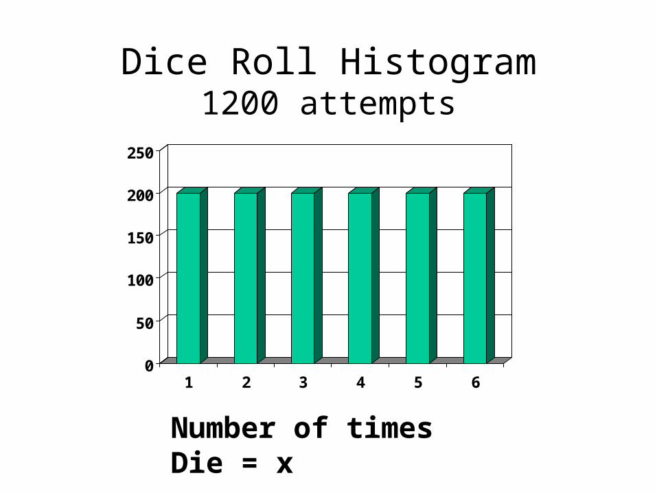
Combining Events• Probability of event not happening:

–

• Probability of both E and F happening:

– IF events E and F are independent

•

• Probability of either E or F happening:

–

]Pr[1Pr EE

]Pr[]Pr[]Pr[Pr FEFEFE

]Pr[]Pr[Pr FEFE

Conditional Probabilities

• The conditional probability that E occurs, given

that F occurs, written Pr[E | F], is defined as

]Pr[

]Pr[]|Pr[

F

FEFE

Conditional Probabilities

• Example: The conditional probability that the

value of a die is 6, given that the value is greater

than 3, is Pr[die=6 | die>3] =

3/12/1

6/1

]3Pr[

]6Pr[

]3Pr[

]36Pr[]3|6Pr[

die

die

die

diediediedie

Probability Pie

Die=1

Die=2

Die=3Die=4

Die=5

Die=6

Conditional Probability Pie

Die=4

Die=5

Die=6

Independence

• Two events E and F are independent if the

probability of E conditioned on F is equal to the

unconditional probability of E. That is, Pr[E | F] =

Pr[E].

• In other words, the occurrence of F has no effect on

the occurrence of E.

Random Variables

• A random variable, R, represents the outcome of

some random event. Example: R = the roll of a die.

• The probability distribution of a random

variable, Pr[R], is a probability measure mapping

each possible value of R into its associated

probability.

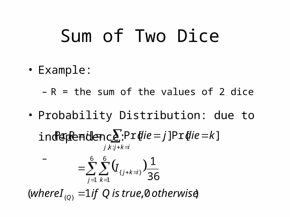
Sum of Two Dice

• Example:

– R = the sum of the values of 2 dice

• Probability Distribution: due to independence:

–

)0,1(

36

1

]Pr[]Pr[]Pr[

}{

6

1

6

1}{

:,

otherwisetrueisQifIwhere

I

kdiejdieiR

Q

j kikj

ikjkj

Sum of Two Dice

...36

3]1Pr[]3Pr[

]2Pr[]2Pr[

]3Pr[]1Pr[]4Pr[36

2]1Pr[]2Pr[

]2Pr[]1Pr[]3Pr[36

1]1Pr[]1Pr[]2Pr[

21

21

21

21

21

21

etc

diedie

diedie

diedieR

diedie

diedieR

diedieR

Probability Mass Function:R = Sum of 2 dice

0

0.1

0.2

0.3

0.4

0.5

2 3 4 5 6 7 8 9 10 11 12

Pr(R = x)

Continuous Random Variables

• So far, we have only considered discrete random

variables, which can take on a countable number

of distinct values.

• Continuous random variables and take on any

real value over some (possibly infinite) range.

– Example: R = Inter-packet-arrival times at a router.

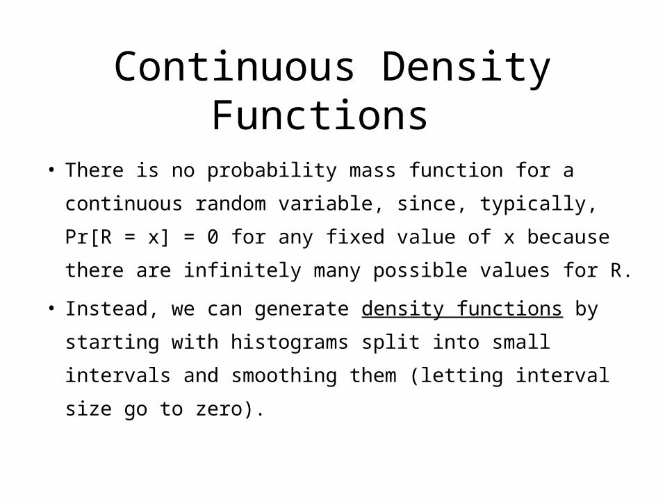
Continuous Density Functions

• There is no probability mass function for a continuous

random variable, since, typically, Pr[R = x] = 0 for any

fixed value of x because there are infinitely many

possible values for R.

• Instead, we can generate density functions by starting

with histograms split into small intervals and smoothing

them (letting interval size go to zero).

Example: Bus Waiting Time

• Example: I arrive at a bus stop at a random time. I

know that buses arrive exactly once every 10

minutes. How long do I have to wait?

• Answer: My waiting time is uniformly

distributed between 0 and 10 minutes. That is, I

am equally likely to wait for any time between 0

and 10 minutes

Bus Wait Histogram2000 attempts (histogram interval = 2 min)

0

200

400

600

0--2 2--4 4--6 6--8 8--10

Waiting Times (using 2-minute ‘buckets’)

Bus Wait Histogram2000 attempts (histogram interval = 1 min)

0

200

400

600

0--1 1--2 2--3 3--4 4--5 5--6 6--7 7--8 8--9 9--10

Waiting Times (using 1-minute ‘buckets’)

Bus Waiting TimeUniform Density Function

0

0.1

0.2

0.3

0.4

0 min. 5 min. 10 min.

110

110

0

dx

Value for Density Function

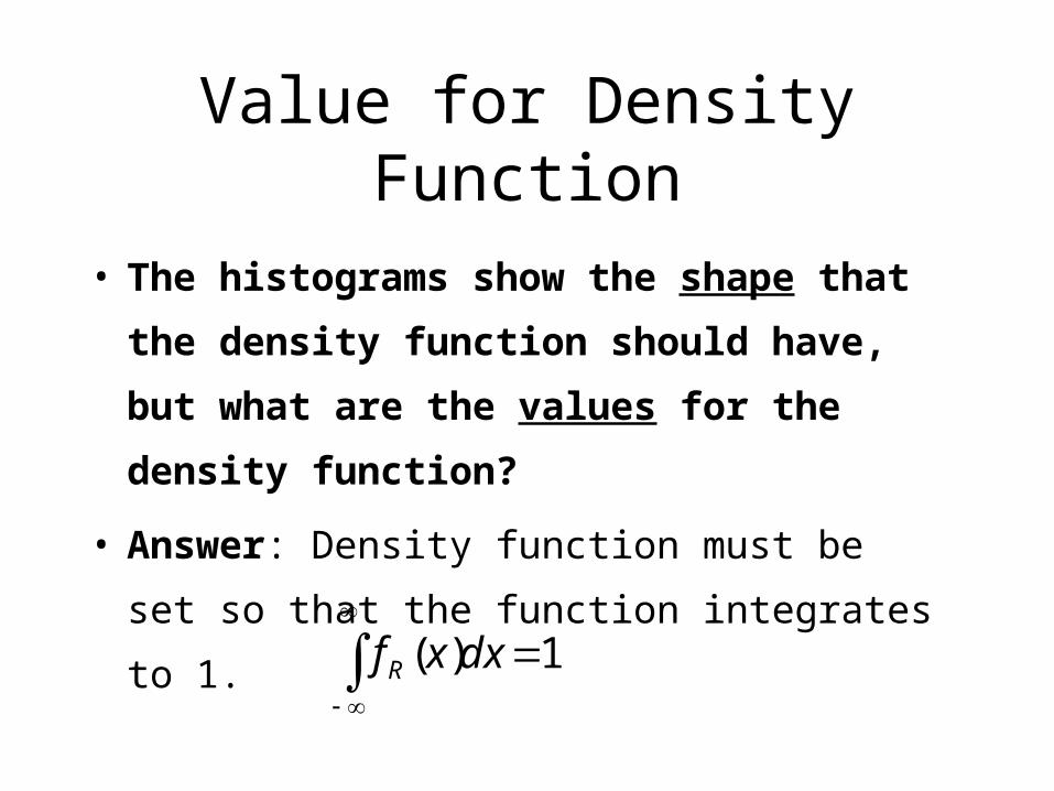
• The histograms show the shape that the

density function should have, but what are the

values for the density function?

• Answer: Density function must be set so that the

function integrates to 1.

1)(

dxxfR

Continuous Density Functions

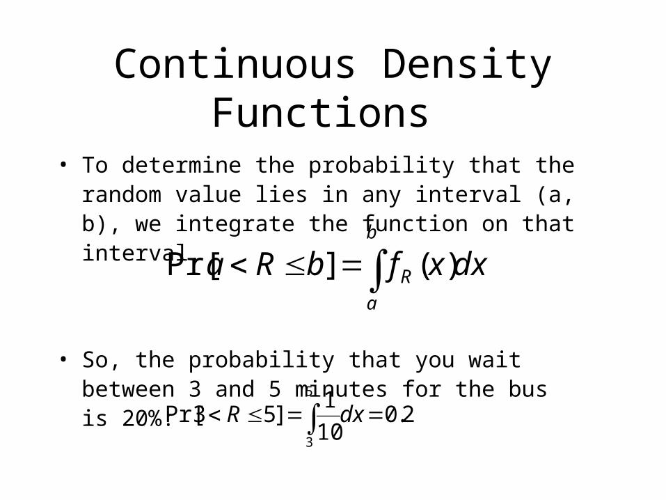
• To determine the probability that the random value lies in any interval (a, b), we integrate the function on that interval.

• So, the probability that you wait between 3 and 5 minutes for the bus is 20%:

dxxfbRab

a

R )(]Pr[

2.010

1]53Pr[

5

3

dxR

Cumulative Distribution Function

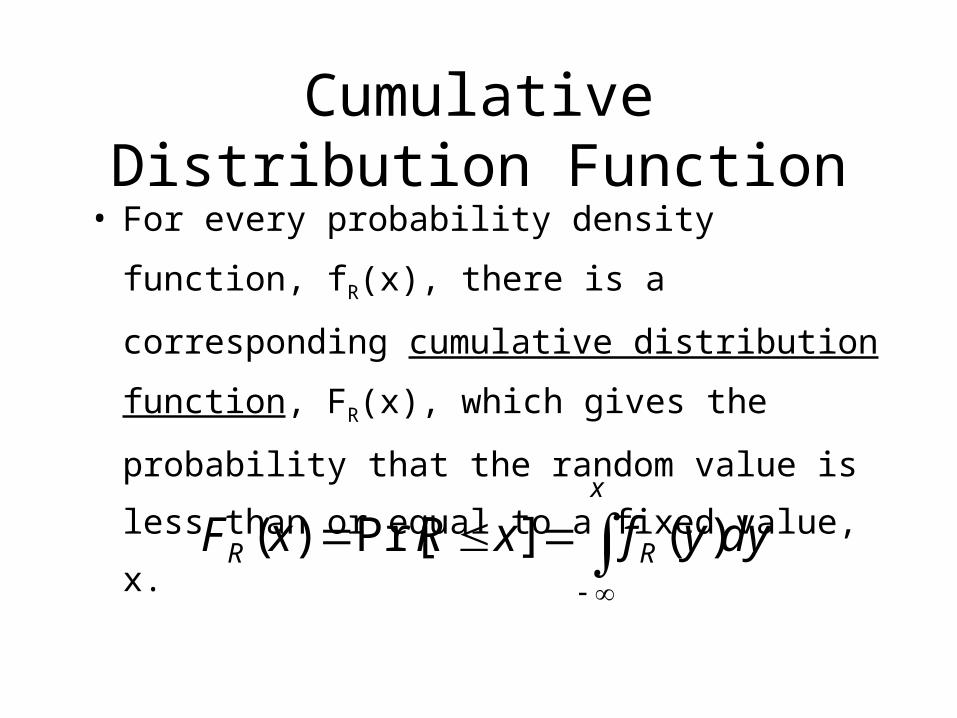
• For every probability density function, fR(x), there

is a corresponding cumulative distribution function,

FR(x), which gives the probability that the random

value is less than or equal to a fixed value, x.

dyyfxRxFx

RR

)(]Pr[)(

Example: Bus Waiting Time

• For the bus waiting time described earlier,

the cumulative distribution function is

1010

1)(

0

xdyxF

x

R

Bus Waiting TimeCumulative Distribution Function

00.10.20.30.40.50.60.70.80.9

1

0 min. 5 min. 10 min.

Pr(R <= x)

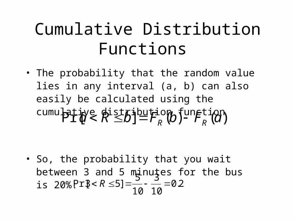
Cumulative Distribution Functions

• The probability that the random value lies in any interval (a, b) can also easily be calculated using the cumulative distribution function

• So, the probability that you wait between 3 and 5 minutes for the bus is 20%:

)()(]Pr[ aFbFbRa RR

2.010

3

10

5]53Pr[ R

Expectation

• The expected value of a random variable, E[R], is

the mean value of that random variable. This may

also be called the average value of the random

variable.

Calculating E[R]

• Discrete R.V.

• Continuous R.V.

x

xRxRE ]Pr[][

dxxxfRE R )(][

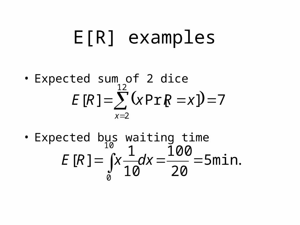
E[R] examples

• Expected sum of 2 dice

• Expected bus waiting time

7]Pr[][12

2

x

xRxRE

.min520

100

10

1][

10

0

dxxRE

Moments

• The nth moment of R is defined to be the expected

value of Rn

– Discrete:

– Continuous:

x

nn xRxRE ]Pr[][

dxxfxRE Rnn )(][

Standard Deviation

• The standard deviation of R, (R), can be defined

using the 2nd moment of R:

22 ])[(][

)()(

RERE

RVarR

Coefficient of Variation

• The coefficient of variation, CV(R), is a common

measure of the variability of R which is

independent of the mean value of R:

][

)(][

RE

RRCV

Coefficient of Variation

• The coefficient of variation for the exponential

random variable is always equal to 1.

• Random variables with CV greater than 1 are

sometimes called hyperexponential variables.

• Random variables with CV less than 1 are

sometimes called hypoexponential variables.

Common Discrete R.V.sBernouli random variable

• A Bernouli random variable w/ parameter p reflects a 2-valued experiment with results of success (R=1) w/ probability p

pR

pR

1]0Pr[

]1Pr[

pRE ][

p

pRCV

1][

Common Discrete R.V.sGeometric random variable

• A Geometric random variable reflects the number

of Bernouli trials required up to and including the

first success

1)1(]Pr[ ippiR

pRE

1][ pRCV 1][

Geometric Mass Function# Die Rolls until a 6 is rolled

0

0.1

0.2

0.3

0.4

0.5

1 2 3 4 5 6 7 8 9 10 11 12

Pr(R = x)

Geometric Cumulative Function# Die Rolls until a 6 is rolled

0

0.2

0.4

0.6

0.8

1

1 2 3 4 5 6 7 8 9 10 11 12

Pr(R <= x)

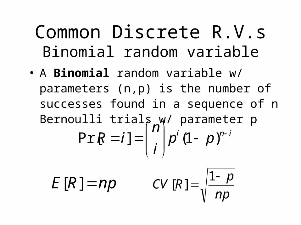
Common Discrete R.V.sBinomial random variable

• A Binomial random variable w/ parameters (n,p) is the number of successes found in a sequence of n Bernoulli trials w/ parameter p

ini ppi

niR

)1(]Pr[

npRE ][np

pRCV

1][

Binomial Mass Function# 6’s rolled in 12 die rolls

0

0.05

0.1

0.15

0.2

0.25

0.3

0.35

0 1 2 3 4 5 6 7 8 9 10 11 12

Pr(R = x)

Common Discrete R.V.sPoisson random variable

• A Poisson random variable w/ parameter models the number of arrivals during 1 time unit for a random system whose mean arrival rate is arrivals per time unit

!]Pr[

ieiR

i

][RE1

][ RCV

Poisson Mass FunctionNumber of Arrivals per second given an average of 4 arrivals per second ( = 4)

0

0.05

0.1

0.15

0.2

0.25

0.3

0.35

0 1 2 3 4 5 6 7 8 9 10 11 12

Pr(R = x)

Continuous R.V.sContinuous Uniform random variable

• A Continuous Uniform random variable is one whose density function is constant over some interval (a,b):

bxaab

xfR

,1

)(

bxaab

axxFR

,)(

2][

abRE

Exponential random variable

• A (Negative) Exponential random variable with parameter represents the inter-arrival time between arrivals to a Poisson system:

0,)( xexf xR

0,1)( xexF xR

Exponential random variable

• Mean (expected value) and coefficient of variation for Exponential random variable:

1

][ RE

1][ RCV

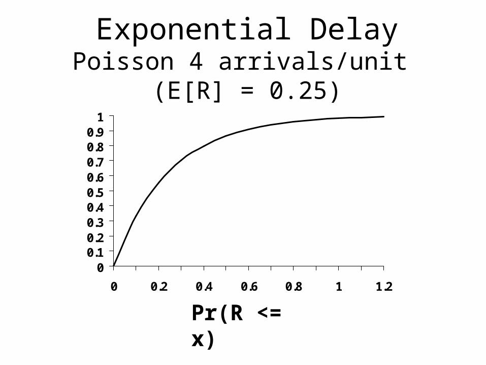
Exponential DelayPoisson 4 arrivals/unit (E[R] = 0.25)

00.10.20.30.40.50.60.70.80.9

1

0 0.2 0.4 0.6 0.8 1 1.2

Pr(R <= x)