TD-DNN: A Time Decay-Based Deep Neural Network ... - MDPI

Citation: Jain, G.; Mahara, T.; Sharma,

S.C.; Agarwal, S.; Kim, H. TD-DNN:

A Time Decay-Based Deep Neural

Network for Recommendation

System. Appl. Sci. 2022, 12, 6398.

https://doi.org/10.3390/app12136398

Academic Editor: Giacomo Fiumara

Received: 19 May 2022

Accepted: 20 June 2022

Published: 23 June 2022

Publisher’s Note: MDPI stays neutral

with regard to jurisdictional claims in

published maps and institutional affil-

iations.

Copyright: © 2022 by the authors.

Licensee MDPI, Basel, Switzerland.

This article is an open access article

distributed under the terms and

conditions of the Creative Commons

Attribution (CC BY) license (https://

creativecommons.org/licenses/by/

4.0/).

applied sciences

Article

TD-DNN: A Time Decay-Based Deep Neural Network forRecommendation SystemGourav Jain 1,* , Tripti Mahara 2, Subhash Chander Sharma 1, Saurabh Agarwal 3 and Hyunsung Kim 4,*

1 Electronics and Computer Discipline, Indian Institute of Technology, Roorkee 247667, India;[email protected]

2 Institute of Management, Christ University, Bengaluru 560029, India; [email protected] Amity School of Engineering & Technology, Amity University Uttar Pradesh, Noida 201313, India;

[email protected] School of Computer Science, Kyungil University, Gyeongsan 38428, Kyungbuk, Korea* Correspondence: [email protected] (G.J.); [email protected] (H.K.)

Abstract: In recent years, commercial platforms have embraced recommendation algorithms toprovide customers with personalized recommendations. Collaborative Filtering is the most widelyused technique of recommendation systems, whose accuracy is primarily reliant on the computedsimilarity by a similarity measure. Data sparsity is one problem that affects the performance of thesimilarity measures. In addition, most recommendation algorithms do not remove noisy data fromdatasets while recommending the items, reducing the accuracy of the recommendation. Furthermore,existing recommendation algorithms only consider historical ratings when recommending the itemsto users, but users’ tastes may change over time. To address these issues, this research presents a DeepNeural Network based on Time Decay (TD-DNN). In the data preprocessing phase of the model,noisy ratings are detected from the dataset and corrected using the Matrix Factorization approach. Apower decay function is applied to the preprocessed input to provide more weightage to the recentratings. This non-noisy weighted matrix is fed into the Deep Learning model, consisting of an inputlayer, a Multi-Layer Perceptron, and an output layer to generate predicted ratings. The model’sperformance is tested on three benchmark datasets, and experimental results confirm that TD-DNNoutperforms other existing approaches.

Keywords: collaborative filtering; deep neural network; noisy ratings; recommendation system; timedecay functions; matrix factorization

1. Introduction

A recommender system (RS) [1,2] is an intelligent system that provides recommenda-tions to users based on their previous ratings. It can easily provide relevant informationto users from massive volumes of Internet data; as a result, it is widely used by manyplatforms to recommend items, movies, music, books, etc. The accuracy of RS mainlydepends upon the recommendation algorithm, which is classified into Content-based (CB),Collaborative Filtering (CF), Demographic-based, Knowledge-based, Community-based, orhybrid [3,4]. The CB technique [5] generates recommendations based on the user and itemprofiles. It has the advantage that it can quickly adjust recommendations in response tochanges in user preferences, but it suffers from a lack of recommendation novelty and coldstart problems and requires a detailed description of items and user profiles. The CF [6]technique is the most popular and commonly used technique of RS, which determinesusers of relevant interest by calculating the similarity, and it recommend items to them. Itmakes accurate recommendations based on user–item interactions such as clicks, browsinghistory, and ratings given. The advantages of the CF technique include scalability and thatit does not require much information about users or items to create a profile. Althoughthis method is simple and effective, its effectiveness drops due to the sparsity problem,

Appl. Sci. 2022, 12, 6398. https://doi.org/10.3390/app12136398 https://www.mdpi.com/journal/applsci

Appl. Sci. 2022, 12, 6398 2 of 22

which increases with the rapid increase in users and items. More importantly, it cannotgenerate recommendations for a new item that has not received user ratings. Therefore,many researchers have begun to look for other ways to improve the recommendationsystem performance. Demographic-based RS [7] provides recommendations based on thedemographic profiles of users’ attributes, i.e., user’s country, education, gender, or age.This technique is not complex and easy to implement, but profiles are rarely updated. InKnowledge-Based RS (KBRS) [8], item recommendations are based on the domain knowl-edge about a user’s needs and preferences. As the recommendations are independent ofthe user ‘s preferences, a KBRS can quickly change its recommendations when a user’sinterest change. The limitation of KBRS is that it must understand the product domain well.Community-based RS [7] suggests items based on the preferences of the user’s friends. Ahybrid recommendation system combines two or more techniques, as discussed above.

In recent years, Deep Learning (DL) [9] has made significant progress and achievednotable success in many sectors such as healthcare [10], cybersecurity [10], natural languageprocessing [11], audio recognition [11], computer vision [12], etc. The promising capabil-ities of DL have encouraged researchers to use deep architecture for recommendationtasks [13,14]. For instance, Cheng et al. [15] introduced a deep architecture for googleplay recommendations, Covington et al. [16] proposed a deep learning-based method forthe YouTube recommendations, and Okura et al. [17] used a Recurrent Neural Networkfor news recommendations. These approaches have displayed remarkable success andoutperformed traditional RS methods.

Developing personalized RS using the Deep Neural Network (DNN) has become apotential trend due to its high computing power and huge data storage capabilities. Thesimplest DNN [13] consists of three layers, i.e., the input layer, the Multi-Layer Perceptron(MLP), and the output layer. The input layer converts low-dimensional features into N-dimensional features and passed them to the MLP layers. In MLP, n-dimensional featuresare learned and passed onto the activation functions of each layer. Finally, the MLP’soutput is passed to the last layer, which predicts the ratings. Some researchers have recentlydeveloped Deep Learning-based recommendation models to improve the system’s accuracy.They make some experimental changes on the MLP layer or the output layer: for instance,changes in the number of layers, activation, or loss function. Two or more approachesare also merged to predict the ratings. However, to the best of our knowledge, thereis no study that performs preprocessing on data before providing it into the DNN. It isimportant because input quality determines output quality. Therefore, the research focuseson preprocessing the original data to improve the input data quality. This is completed asfollows: (1) identifying the dataset’s noisy (inconsistent) ratings and correcting them usingthe matrix factorization approach; and (2) assigning weightage to the recent ratings usingthe time function, i.e., Power. The resultant data matrix is provided as the input into theDNN model for training purposes. The embedding layers are used in the DNN becausethey reduce the input size and computational complexity, leading to faster training times.

As such, we summarize the contributions as follows:

1. In this paper, a Time Decay-based Deep Neural Network (TD-DNN) is proposed, inwhich, firstly, the noisy ratings are identified from the dataset and corrected using theMatrix Factorization approach. After this, to give the weightage to the most recentratings, a power decay function is used. The resultant data matrix is inserted as theinput into the DNN model for the training purposes.

2. The model incorporates the embedding layer to a Multi-Layer Perceptron to learn theN-dimensional and non-linear interactions between users and movies. The Huberloss function, which has shown outstanding efficacy across all the loss functions, isused.

3. The experiment has been conducted on benchmark datasets to examine the newmodel’s efficiency and compare it with the existing approaches. The results on theMovieLens-100k, ML-1M and Epinions datasets show that the proposed TD-DNN ar-chitecture enhances recommendation efficiency and solves the data sparsity problem.

Appl. Sci. 2022, 12, 6398 3 of 22

The paper is organized as follows: The literature review is examined in Section 2,which is followed by the problem statement discussed in Section 3. The proposed modelis evaluated in Section 4, and the results are presented in Section 5. The paper comes to aconclusion in Section 6.

2. Literature Review

This section discusses the state-of-the-art techniques used in recommendation systems.The collaborative filtering technique-based recommendation algorithms are discussed first,which is followed by the deep learning techniques for recommendation.

The collaborative filtering technique considers historical data to recommend items tothe target users. It is mainly categorized into memory-based and model-based techniques.Out of these two, the memory-based approach is most popular and is subdivided intouser-based [18] and item-based [19] approaches. Many similarity measures, i.e., ModifiedProximity Impact Popularity (MPIP) [20], RJaccard [21], TMJ [22], etc., have been intro-duced in recent years. The CF approach is popular because it is simple to implement;nonetheless, it suffers from a data sparsity problem. Many model-based algorithms, such asBayesian models [23], Latent Semantic models [24], Regression-based models [25], MatrixFactorization models [26], etc., have been proposed to overcome the challenge mentionedabove. Among these models, the most prominent is Matrix Factorization, which mapsthe users and items into vectors representing the users’ or items’ latent features. Somevariants of the Matrix Factorization (MF) model are Nonparametric Probabilistic PrincipalComponent Analysis (NPCA) [27], Singular Value Decomposition (SVD) [28], and Proba-bilistic Matrix Factorization (PMF) [29]. The latent features learned by matrix factorizationapproaches are ineffective when the rating matrix is highly sparse. In addition, numerousresearchers construct an effective recommendation system using additional data, such astime, trust, and location information. For instance, the authors in [30] utilized the user’strust and location information to improve the prediction accuracy of RS. Some researchersincorporated time information at the similarity computation [31], prediction [32], or ratingmatrix levels [33] of the recommendation process.

On the other hand, deep learning [34] is a growing field of machine learning researchthat mimics the human brain’s behavior for interpreting data such as images, sounds, andtexts. It is a Multi-Layer Perceptron with multiple hidden layers stacked on each other.Hinton et al. [35] introduced the concept of Deep Learning and proposed an unsuper-vised algorithm based on deep belief networks (DBN). These Deep Learning techniqueshave recently succeeded in many complex tasks, i.e., computer vision, natural languageprocessing, etc. Therefore, researchers have begun to apply Deep Learning algorithms torecommending music [36], books [11], videos [16], medical [37], interfaces [38], etc. Thefirst Deep Learning-based recommendation model was Neural Collaborative Filtering(NCF) [39], which targets the poor representation of MF in a low-dimensional space andreplaces it with neural network architecture. Since MF is a popular technique used in RS,several works have been proposed using Matrix Factorization and Deep Neural Networks.Xue et al. [40] proposed a Deep Matrix Factorization (DMF) model in which features areextracted from the user–item matrix and integrated into the neural network. The authoralso proposed a new loss function based on binary cross-entropy to minimize the error. Anew approach based on personalized Long and Short-Term Memory (LSTM) and MatrixFactorization techniques is presented in [41]. In [42], the authors developed an improvedmatrix factorization technique. A movie recommendation system that predicted the Top-Nrecommendation list of movies using singular value decomposition and cosine similarity isproposed in [43]. In the Deep Learning model for a Collaborative Recommender System(DLCRS) [44], user and movie IDs are concatenated as one-hot vectors. Unlike the basic MFapproach, where inner products combine the user and movie ratings, DLCRS performs theelement-wise multiplication of user and movie ratings. A novel recommendation strategybased on Artificial Neural Networks and Generalized Matrix Factorization is proposedby Kapetanakis et al. [45]. It improves the overall quality of the recommendations and

Appl. Sci. 2022, 12, 6398 4 of 22

minimizes human intervention and offline evaluations. Wang et al. [46] propose a hierar-chical Bayesian model to obtain content features and a traditional CF model to address therating information. A ConvMF model, which combines the Convolution Neural Networkwith the Probabilistic Matrix Factorization, is proposed in [47]. Some more studies on therecommendation system are given in [13,34].

3. Motivation

Among the various approaches used to develop the recommendation systems, thememory-based Collaborative Filtering technique is most popular and widely used, but ithas some limitations as discussed below.

In the CF approach, the efficiency of the RS mainly depends upon finding the effectiveneighbors which are based on the similarity calculated by a similarity measure. There arevarious traditional and recently developed similarity measures, but they mainly suffer fromthe sparsity, cold- start and scalability problems. Some traditional and popular similaritymeasures in the CF technique compute incorrect similarity in some cases. For instance, thecosine measure [48,49] computes the maximum similarity between users when they haveonly rated only one item. Pearson Correlation Coefficient (PCC) calculates low similarityregardless of the similar ratings of two users. The Jaccard measure [49] does not count theabsolute values of ratings, while the Mean Squared Difference (MSD) measure ignores theproportion of common ratings. The combination of these two is JMSD, which does notutilize all the ratings provided by both users. Some recently developed similarity measures,i.e., Relevant Jaccard (RJaccard) and Relevant Jaccard MSD (RJMSD), compute inaccuratesimilarity when the user rates the items with equal ratings. In addition, the accuracy ofthe CF techniques is also affected when some inconsistency/noisy ratings [50] exist in thedataset. In this case, similarity measures compute inaccurate similarity. These existingCF algorithms only consider the historical ratings when computing similarity, but as timegoes by, users’ tastes may change; therefore, the generated recommendation might notbe relevant.

To address the aforementioned problems and improve the performance of recommen-dation systems, a Time Decay-based Deep Neural Network (TD-DNN) has been proposedin this paper. In this, firstly, we do some preprocessing on data to remove noise and giveweightage to the most recent ratings. For correcting the noisy ratings, the Matrix Factor-ization approach is used, while the power decay function is used to give weightage to themost recent ratings. The resultant data matrix is inserted as the input into the DNN modelfor training purposes, and it produces the predicted ratings as output.

4. Proposed Methodology

Deep Learning [51] (also known as deep artificial neural networks) learns the latentfeatures of users and movies and inserts them as input into a multi-layered feed-forwardarchitecture to predict the ratings as output. DNN can learn the complex decision bound-aries for classification and non-linear regression. A typical deep neural network has threedistinct functional layers [12]: the input layer, Multi-Layer Perceptron (MLP), and theoutput layer. The output of each layer is promoted to the next layer in a multi-layer neuralnetwork. For example, the output of the input layer is of user and item vectors, whichare sent to a Multi-Layer Perceptron. The MLP has large numbers of hidden layers andis used to train the obtained N-dimensional non-linear features, and the output of this isforwarded to the last layer to forecast the ratings. Unlike other Deep Learning models,where the original/raw data matrix is inserted as input into the input layer of the model, theproposed model takes into consideration a preprocessed data matrix. In the preprocessingstep, first, the noisy ratings are detected and corrected, and then, a time decay function isapplied to give weightage to the recent ratings. The resultant matrix is fed into the neuralnetwork model to predict the ratings. The development of the proposed model constitutestwo phases.

Appl. Sci. 2022, 12, 6398 5 of 22

1. Data Preprocessing Phase2. Constructing Deep Neural Network

The detailed description of each phase is given below.

4.1. Data Preprocessing Phase

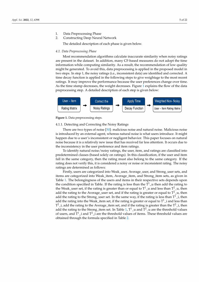
Most recommendation algorithms calculate inaccurate similarity when noisy ratingsare present in the dataset. In addition, many CF-based measures do not adopt the timeinformation while computing similarity. As a result, the recommendation of low qualitymight be generated. To avoid this, data preprocessing is applied in the proposed model intwo steps. In step 1, the noisy ratings (i.e., inconsistent data) are identified and corrected. Atime decay function is applied in the following steps to give weightage to the most recentratings. It may improve the performance because the user preferences change over time.As the time stamp decreases, the weight decreases. Figure 1 explains the flow of the datapreprocessing step. A detailed description of each step is given below:

Figure 1. Data preprocessing steps.

4.1.1. Detecting and Correcting the Noisy Ratings

There are two types of noise [50]: malicious noise and natural noise. Malicious noiseis introduced by an external agent, whereas natural noise is what users introduce. It mighthappen due to a user’s inconsistent or negligent behavior. This paper focuses on naturalnoise because it is a relatively new issue that has received far less attention. It occurs due tothe inconsistency in the user preference and item ratings.

To identify natural noise/noisy ratings, the user, item, and ratings are classified intopredetermined classes (based solely on ratings). In this classification, if the user and itemfall in the same category, then the rating must also belong to the same category. If therating does not verify this, it is considered a noisy or noise or inconsistent rating. The noisyratings are determined as follows:

Firstly, users are categorized into Weak_user, Average_user, and Strong_user sets, anditems are categorized into Weak_item, Average_item, and Strong_item sets, as given inTable 1. The belongingness of the users and items in their respective sets depends uponthe condition specified in Table. If the rating is less than the T1_u then add the rating tothe Weak_user set, if the rating is greater than or equal to T1_u and less than T2_u, thenadd the rating to the Average_user set, and if the rating is greater or equal to T2_u, thenadd the rating to the Strong_user set. In the same way, if the rating is less than T1_i, thenadd the rating into the Weak_item set, if the rating is greater or equal to T1_i and less thanT2_i, add the rating to the Average_item set, and if the rating is greater than the T2_i, thenadd the rating to the Strong_item set. In Table 1, T1_u and T2_u are the threshold valuesof users, and T1_i and T2_i are the threshold values of items. These threshold values areobtained through the formula specified in Table 2.

Appl. Sci. 2022, 12, 6398 6 of 22

Table 1. Categorized Users and Items into Sets.

Users Sets

If r (user, item) < T1_u add rating into Weak_user setIf r (user, item) ≥ T1_u and r (user, item) < T2_u add rating into Average_user setIf r (user, item) ≥ T2_u add rating to the Strong_user set

Item Sets

If r (user, item) < T1_i add rating into Weak_item setIf r (user, item) ≥ T1_i and r (user, item) < T2_i add rating into Average_item setIf r (user, item) ≥ T2_i add rating into Strong_item set

Table 2. Thresholds.

Thresholds Formula

T1_u or T1_i or T1 Rmin + round (1/3 × (Rmax − Rmin)T2_u, or T2_i or T2 Rmax − round (1/3 × (Rmax − Rmin)

In Table 2, Rmin and Rmax are the minimum and maximum values in the rating scale,respectively. After determining the threshold values, the users, items, and ratings areclassified into three categories, as displayed in Table 3. In the table, users are classifiedinto Critical, Average, and Benevolent. Items are classified into Weakly recommended,Averagely recommended, and Strongly recommended, and ratings are classified into Weak,Average, and Strong. A critical user is the one who gives a low rating to items, an averageuser provides the average rating to items, and a benevolent user is the one who givesa high rating to items. Similarly, if the majority of people dislike the item, it is Weaklyrecommended, and if the majority of users averagely like it, it is Averagely recommended.If most users prefer the item, it is categorized as Strongly recommended. Similarly, if therating is less than T1 (threshold value), it is a Weak rating. If the rating is greater or equalto T1 and less than T2, it is an Average rating, and if the rating is greater than T2, it is aStrong rating.

Table 3. User, Item and Rating Classes.

User Classes

If |Weak_user| ≥ |Strong_user| + |Average_user| User is CriticalIf |Average_user| ≥ |Strong_user| + |Weak_user| User is AverageIf |Strong_user| ≥ |Average _user| + |Weak_user| User is Benevolent

Item Classes

If |Weak_item| ≥ |Strong_item| + |Average_item| Item is Weakly recommendedIf |Average_item| ≥ |Strong_item| + |Weak_item| Item is Averagely recommendedIf |Strong_item| ≥ |Average_item| + |Weak_item| Item is Strongly recommended

Rating Classes

If r (user, item) < T1 Rating is WeakIf T1 ≤ r (user, item) < T2 Rating is AverageIf r (user, item) ≥ T2 Rating is Strong

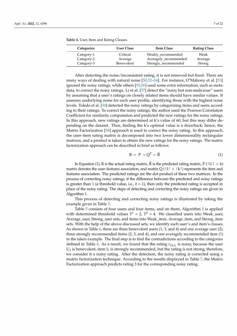
Table 4 defines the three categories of homologous classes according to the classes ofusers, items, and ratings defined in Table 3. If the classes associated with the user and itemare similar, then the ratings must also belong to a similar category. If this does not happen,we can say that the rating is noisy. For example, if the user is strong, the item is stronglyrecommended, and if the rating is average, we can say that the rating is noisy.

Appl. Sci. 2022, 12, 6398 7 of 22

Table 4. User, Item and Rating Classes.

Categories User Class Item Class Rating Class

Category-1 Critical Weakly_recommended WeakCategory-2 Average Averagely_recommended AverageCategory-3 Benevolent Strongly_recommended Strong

After detecting the noise/inconsistent rating, it is not removed but fixed. There aremany ways of dealing with natural noise [50,52–54]. For instance, O’Mahony et al. [53]ignored the noisy ratings, while others [55,56] used some extra information, such as meta-data, to correct the noisy ratings. Li et al. [57] detect the “noisy but non-malicious” usersby assuming that a user’s ratings on closely related items should have similar values. Itassesses underlying noise for each user profile, identifying those with the highest noiselevels. Toledo et al. [50] detected the noisy ratings by categorizing items and users accord-ing to their ratings. To correct the noisy ratings, the author used the Pearson CorrelationCoefficient for similarity computation and predicted the new ratings for the noisy ratings.In this approach, new ratings are determined at k’s value of 60, but this may differ de-pending on the dataset. Thus, finding the k’s optimal value is a drawback; hence, theMatrix Factorization [58] approach is used to correct the noisy rating. In this approach,the user–item rating matrix is decomposed into two lower dimensionality rectangularmatrices, and a product is taken to obtain the new ratings for the noisy ratings. The matrixfactorization approach can be described in brief as follows:

R = P ×QT = R (1)

In Equation (1), R is the actual rating matrix, R is the predicted rating matrix, P (|U| × k)matrix denotes the user–features association, and matrix Q (|I| × |k|) represents the item andfeatures association. The predicted ratings are the dot product of these two matrices. In theprocess of correcting noisy ratings, if the difference between the predicted and noisy ratingsis greater than 1 (a threshold value, i.e., δ = 1), then only the predicted rating is accepted inplace of the noisy rating. The steps of detecting and correcting the noisy ratings are given inAlgorithm 1.

This process of detecting and correcting noisy ratings is illustrated by taking theexample given in Table 5.

Table 5 consists of four users and four items, and on them, Algorithm 1 is appliedwith determined threshold values T1 = 2, T2 = 4. We classified users into Weak_user,Average_user, Strong_user sets, and items into Weak_item, Average_item, and Strong_itemsets. With the help of the above-discussed sets, we identify each user’s and item’s classes.As shown in Table 6, there are three benevolent users (1, 3, and 4) and one average user (2),three strongly recommended items (2, 3, and 4), and one averagely recommended item (1)in the taken example. The final step is to find the contradictions according to the categoriesdefined in Table 4. As a result, we found that the rating rU2 I1 is noisy, because the userU2 is benevolent, item I1 is strongly recommended, but the rating is not strong; therefore,we consider it a noisy rating. After the detection, the noisy rating is corrected using amatrix factorization technique. According to the results displayed in Table 7, the MatrixFactorization approach predicts rating 3 for the corresponding noisy rating.

Appl. Sci. 2022, 12, 6398 8 of 22

Algorithm 1: Steps of Detecting and Correcting Noisy Ratings

Inputs: set of available ratings {r(user, item)},Threshold for Classification—T1_u, T2_u, T1_i, T2_i, T_u, T_i, δ = 11. Weak_user = {}, Average_user = {}, Strong_user = {},2. Weak_item = {}, Average _item = {}, Strong_item = {},3. Possible_noise = {}4. for each rating in set of available ratings r(user, item)5. if r(user, item) < T1_u6. Add r(user, item) to the Weak_user set7. else if r(user, item) ≥ T1_u and r(user, item) < T2_u8. Add r(user, item) to the Average_user set9. else10. Add r(user, item) to the Strong_user set11. if r(user, item) < T1_i,12. Add r(user, item) to the Weak_item set13. else if r(user, item) ≥ T1_i, and r(user, item) < T2_i14. Add r(user, item) to the Average_item set15. else16. Add r(user, item) to the Strong_item set17. end for18. for each user in the r(user, item)19. Classify each user into Critical, Average and Strong user as follows:20. Critical user:21. if |Weak_user| ≥ |Strong_user| + |Average_user|22. Average user:23. if |Average_user| ≥ |Strong_user| + |Weak_user|24. Strong user:25. if |Strong_user| ≥ |Average_user| + |Weak_user|26. end for27. for each item in the r(user, item)28. Classify each item using the above discussed sets29. Critical items:30. if |Weak_item| ≥ |Strong_item| + |Average_item|31. Average item:32. if |Average_item| ≥ |Strong_item| + |Weak_item|33. Strong item:34. if |Strong_item| ≥ |Average_item| + |Weak_item|35. end for36. for each rating r(user, item)37. if user is Critical, item is Weakly_recommended, and r(user, item) ≥ T1

38. Add r(user, item) to the {Possible_noise}39. if user is Average, item is Averagely_recommended and (r(user, item) < T1orr(user, item) ≥ T2)40. Add r(user, item) to the {Possible_noise}41. if user is Benevolent, item is Strongly_recommended, and r(user, item) < T2

42. Add r(user, item) to the {Possible_noise}43. end for#Correct the noisy ratings44. for each rating r(user, item) in {Possible_noise}, predict a new rating R(user, item) usingMatrix Factorization approach45. k = 3 # it represents the features46. if (abs (R(user, item) − r(user, item)) > δ)47. Replace r(user, item) by R(user, item) in the original rating set r48. end if49. end for

Output: r = {r(user, item)} − set of corrected ratings

Appl. Sci. 2022, 12, 6398 9 of 22

Table 5. An Example.

I1 I2 I3 I4

U1 3 5 4 4U2 2 5 4 4U3 3 3 2 5U4 4 4 - 1

Table 6. User and Item Classification for the Given Example.

Classification Users |Weak_User| |Average_User| |Strong_User| Class

Users

U1 0 1 3 BenevolentU2 1 0 3 BenevolentU3 1 0 2 AverageU4 1 0 3 Benevolent

Items |Weak_item| |Average_item| |Strong_item| Class

Items

I1 1 2 1 Averagely recommendedI2 0 1 3 Strongly recommendedI3 1 0 2 Strongly recommendedI4 1 0 3 Strongly recommended

Table 7. Corrected Ratings for the Given Example.

I1 I2 I3 I4

U1 3 5 4 4U2 3 5 4 4U3 3 3 2 5U4 4 4 - 1

4.1.2. Applying Time Decay Functions

The CF technique-based algorithms provide recommendations based on the user’shistorical rating data, but the user’s interest changes with time. Therefore, to give weightageto the most recent ratings, a time decay function [59] is incorporated with ratings. Thesetime functions [60–62] determine the appropriate time weights and provide high weightageto the recently rated items. In Table 8, a list of time decay functions is given, and they areapplied to the ML-100k dataset to identify the best option. The results are displayed in thenext section.

Table 8. List of Time Decay Functions.

Function Mathematical Expression References

Exponential e−µ|Tua ,k | [31,63]Concave α|Tua ,k | [62]Convex 1− βt−|Tua ,k | [62]Linear 1− |Tua ,k |

t .γ [62]Logistic 1

1+e−λ∗ |Tua ,k |[33,59]

Power∣∣Tua ,k

∣∣− ω [59]

Here, µ, α, β, ω, γ and λ are the tuning parameter, while t is the difference betweenthe recent timestamp and timestamp at which item is rated.

The first time-based recommendation algorithm was developed by Zimdars et al. [64],who reframed the recommendation issue as a time series prediction problem. In CF, timedecay functions can be applied at the similarity computation, prediction, or rating matrixlevels. Since we are not predicting the ratings using a similarity measure in this paper, we

Appl. Sci. 2022, 12, 6398 10 of 22

can apply these time functions at the rating matrix level only. Here, the ratings closer tothe current time are given a larger weighting coefficient. The time-weighted ratings can beretrieved as follows

Ru,i = ru,i × Time Decay Function (2)

where Ru,i is the predicted rating, ru,i is the actual ratings, and the time decay functionsare listed in Table 8. The results of time functions are displayed in Section 5.5, clearlystating that the performance of the power decay function is superior; hence, it is used inthe research. With the help of the power time function, firstly, weights are computed andthen multiplied with the non-noisy rating dataset to give weightage to the most recentratings. Here, high weightage is assigned to recent timestamp ratings. The resultant non-noisy-time weighted (NNTW) ratings are fed into the Deep Neural Network to improvethe recommendation system performance further. A brief description of the DNN model isgiven below.

4.2. Constructing Deep Neural Network

A Deep Neural Network (DNN) [65] is an Artificial Neural Network with severallayers between the input and output layers. These neural networks come in various shapesand sizes, but they all have the same fundamental components: neurons, weights, biases,and functions. A typical DNN consists of three layers: an input layer, MLP, and outputlayer. The description of each layer is given below.

4.2.1. Input Layer

Every Deep Neural Network architecture relies heavily on its input layer, whoseprincipal function is to process the data that has been provided. Unlike other Deep Learningmodels, where the raw data matrix is provided in the input layer, we provided a Non-NoisyTime Weighted (NNTW) rating matrix (that we obtained from the previous step) to theinput layer. In this layer, there are two input vectors Vu (for user u) and Vi (for item i). Afterthe input layer, there is an embedding layer with a bias term which is a fully connected layerthat turns a sparse vector into a dense one. The produced embedding may be considered asthe user/item latent vector that are concatenated to create an effective deep learning-basedrecommender system.

x0 = concatenate(vu, vi) (3)

In Equation (3), the concatenate function () joins two vectors, i.e., users and movies.The x0 is passed to the first hidden layer of MLP, whose description is given below.

4.2.2. Multi-Layer Perceptron

A feed-forward neural network with several (one or more) hidden layers betweenthe input and output layers is called the Multi-Layer Perceptron (MLP). Since a simplevector concatenation is insufficient to represent the interactions between the user’s andthe item’s latent features, MLP is used. It add hidden layers to the concatenated vector toeasily modulate the non-linear interactions between users and items.

This work learns the N-dimensional non-linear connection between users and movievectors by a fully connected Multi-Layer Perceptron (MLP) architecture. We may utilizefunctions such as sigmoid, hyperbolic tangent (tanh), and Rectified Linear Unit (ReLU)to activate neurons in MLP layers, but each has its restrictions. For instance, the sigmoidfunction does not have a zero-centric function, which may reduce the model’s efficiency. Italso suffers from a gradient vanishing problem. The tanh function, which has a zero-centricfunction, is a rescaled variant of the sigmoid activation function. It is more computationallyexpensive than the sigmoid function. Therefore, it is also not appropriate. On the otherhand, the ReLU activation function has no gradient vanishing problem and is less expensive.In addition, it is well suited for sparse datasets and makes Deep Neural Networks tenableto be overfitting; hence, it is used. To prevent the model from overfitting, L2 Regularizer is

Appl. Sci. 2022, 12, 6398 11 of 22

applied. Each neural network architecture follows the standard tower structure; there aremore neurons at lower levels and fewer at higher levels [66].

In the MLP’s forward propagation process, the first hidden layer output is obtainedby the following equation:

x1 = activation (W1x0 + b1) (4)

where x0 is the input layer’s output, W1 denotes the weight between the input and firsthidden layers, and b1 denotes a bias vector. The activation function makes a non-linear andmeaningful neural network. The ReLU [12,67] activation function is used since it is moreeffective and easier to tune. The following is the output of the lth hidden layer:

xl = ReLU (Wl xl−1 + bl) (5)

The predicted ratings are determined by the size of the final hidden layer, whichindicates the model’s capabilities.

4.2.3. Output Layer

The aim of TD-DNN is to predict the user’s rating in the output layer, using theequation below:

Ru,i = sigmoid(Woutxh + bout) (6)

where Ru,i represents the predicted rating of user u for an item i, h represents the numberof hidden layers, xh is the last hidden layer output, and Wout and bout represent the weightand bias of the output layer, respectively. In Equation (6), the sigmoid activation functionis applied to the last layer. The Huber loss function is used in the training process toevaluate the difference between the predicted ratings Ru,i and actual rating ri,j. The Adamoptimizer is used to modify the weight, which helps reduce the overall loss and improvesaccuracy. The Huber loss function and Adam optimizer are described in the next section.The architecture of our Deep Neural Network is displayed in Figure 2.

Figure 2. Architecture of our Deep Neural Network model.

4.2.4. Training Process

Our proposed deep learning model includes the data preprocessing step in the basicneural network architecture. The Deep Learning architectures compare the predictedratings with the actual ones and constantly refine the target loss to achieve the final optimalfit. In the training of every neural network model, the loss function and optimizer are veryimportant, which are described below:

Loss Functions

The loss function measures the difference between the actual output and the model’spredicted output. Selecting an appropriate loss function is most important. There are mainlytwo types of loss function [11]: pointwise and pairwise loss function. The recommendersystems problem is transformed into a multi-classification or regression problem using apointwise loss function. In contrast, the problem is transformed into a binary classificationproblem using a pairwise loss function. The pointwise loss functions include classification

Appl. Sci. 2022, 12, 6398 12 of 22

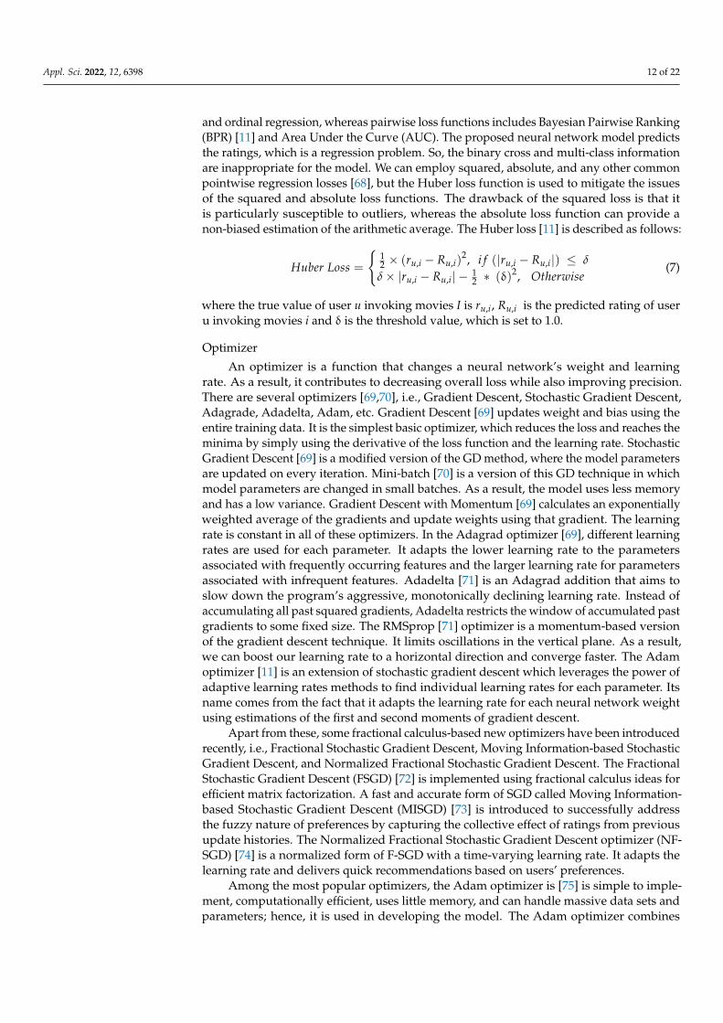
and ordinal regression, whereas pairwise loss functions includes Bayesian Pairwise Ranking(BPR) [11] and Area Under the Curve (AUC). The proposed neural network model predictsthe ratings, which is a regression problem. So, the binary cross and multi-class informationare inappropriate for the model. We can employ squared, absolute, and any other commonpointwise regression losses [68], but the Huber loss function is used to mitigate the issuesof the squared and absolute loss functions. The drawback of the squared loss is that itis particularly susceptible to outliers, whereas the absolute loss function can provide anon-biased estimation of the arithmetic average. The Huber loss [11] is described as follows:

Huber Loss =

{12 × (ru,i − Ru,i)

2, i f (|ru,i − Ru,i|) ≤ δ

δ× |ru,i − Ru,i| − 12 ∗ (δ)2, Otherwise

(7)

where the true value of user u invoking movies I is ru,i, Ru,i is the predicted rating of useru invoking movies i and δ is the threshold value, which is set to 1.0.

Optimizer

An optimizer is a function that changes a neural network’s weight and learningrate. As a result, it contributes to decreasing overall loss while also improving precision.There are several optimizers [69,70], i.e., Gradient Descent, Stochastic Gradient Descent,Adagrade, Adadelta, Adam, etc. Gradient Descent [69] updates weight and bias using theentire training data. It is the simplest basic optimizer, which reduces the loss and reaches theminima by simply using the derivative of the loss function and the learning rate. StochasticGradient Descent [69] is a modified version of the GD method, where the model parametersare updated on every iteration. Mini-batch [70] is a version of this GD technique in whichmodel parameters are changed in small batches. As a result, the model uses less memoryand has a low variance. Gradient Descent with Momentum [69] calculates an exponentiallyweighted average of the gradients and update weights using that gradient. The learningrate is constant in all of these optimizers. In the Adagrad optimizer [69], different learningrates are used for each parameter. It adapts the lower learning rate to the parametersassociated with frequently occurring features and the larger learning rate for parametersassociated with infrequent features. Adadelta [71] is an Adagrad addition that aims toslow down the program’s aggressive, monotonically declining learning rate. Instead ofaccumulating all past squared gradients, Adadelta restricts the window of accumulated pastgradients to some fixed size. The RMSprop [71] optimizer is a momentum-based versionof the gradient descent technique. It limits oscillations in the vertical plane. As a result,we can boost our learning rate to a horizontal direction and converge faster. The Adamoptimizer [11] is an extension of stochastic gradient descent which leverages the power ofadaptive learning rates methods to find individual learning rates for each parameter. Itsname comes from the fact that it adapts the learning rate for each neural network weightusing estimations of the first and second moments of gradient descent.

Apart from these, some fractional calculus-based new optimizers have been introducedrecently, i.e., Fractional Stochastic Gradient Descent, Moving Information-based StochasticGradient Descent, and Normalized Fractional Stochastic Gradient Descent. The FractionalStochastic Gradient Descent (FSGD) [72] is implemented using fractional calculus ideas forefficient matrix factorization. A fast and accurate form of SGD called Moving Information-based Stochastic Gradient Descent (MISGD) [73] is introduced to successfully addressthe fuzzy nature of preferences by capturing the collective effect of ratings from previousupdate histories. The Normalized Fractional Stochastic Gradient Descent optimizer (NF-SGD) [74] is a normalized form of F-SGD with a time-varying learning rate. It adapts thelearning rate and delivers quick recommendations based on users’ preferences.

Among the most popular optimizers, the Adam optimizer is [75] is simple to imple-ment, computationally efficient, uses little memory, and can handle massive data sets andparameters; hence, it is used in developing the model. The Adam optimizer combines

Appl. Sci. 2022, 12, 6398 13 of 22

two gradient descent methodologies [76]: Momentum and RMSProp, with Momentumproviding smoothing and RMSProp efficiently changing the learning rate.

The weight and bias update in Momentum are given by:

w = w− α·vdwb = b− α· vdb (8)

The weight and bias update in RMSProp are given by:

w = w− α ·((∂L/∂w)/

√sdw + ε

)b = b− α·

((∂L/∂b)/

√sdb + ε

)(9)

where w and b are the weights and bias, respectively, vdw is the sum of gradients ofweights at time t, vdb is the sum of gradients of bias at time t, sdw is the sum of square ofpast gradients of weights, sdb is the sum of square of the past gradients of bias, ∂L is thederivative of loss function, ∂w is the derivatives of weight at time t, and ∂w is the derivativeof bias. Initially, vdw, sdw, vdb and sdb all are set to zero. On iteration t, they are computedas follows.

vdw = β1 vdwt−1 + (1− β1)∂L∂w

vdb = β1 vdbt−1 + (1− β1)∂L∂b

sdw = β2 vdwt−1 + (1− β2)(

∂L∂w

)2

sdb = β2 vdbt−1 + (1− β2)(

∂L∂b

)2

(10)

In Momentum and RMSProp, initially, vdw, sdw, vdb and sdb were initialized to 0,but it is observed that they become 0 when both β1 and β2 are near to 1. The Adamoptimizer [76] fixed this issue by using the corrected formula as given below. This is alsocompleted to keep the weights under control when they approach the global minimum.The corrected formulas for vdw, sdw, vdb and sdb are given below:

vcorrecteddw = vdw

1−βt1

vcorrecteddb = vdb

1−βt1

scorrecteddw = sdw

1−βt2

scorrecteddb = sdb

1−βt2

(11)

Put these correct values in Equation (12) to compute the weight and bias in Adam optimizer.

wt = wt−1 + ηvcorrected

dw√scorrected

dw +ε

bt = bt−1 + ηvcorrected

db√scorrected

db +ε

(12)

where wt and wt−1 are the weights at time t and t− 1, respectively. β1 (=0.9) and β2 (=0.999)are the moving average parameters, ε, usually of the order of 1 × 10−8 and η is a learningrate, whose best values is tuned by performing experiments.

5. Experimental Evaluation5.1. Data Description

Three real-world datasets [4,18] are taken to evaluate the performance of the proposedNN model: MovieLens-100k, MovieLens-1M, and Epinions. The MovieLens-100k dataset(http://grouplens.org/datasets/movielens/100k, 28 December 2022) was generated by theUniversity of Minnesota’s Group Lens Research Group. In this, every user assessed at least20 films on a scale of one to five, with one being the worst and five being the best rated.

Another dataset is MovieLens-1M (http://grouplens.org/datasets/movielens/1m,1 January 2022), in which users rated at least twenty items. We employed the Epinionsdataset (http://www.trustlet.org/epinions.html, 1 January 2022) to evaluate the proposed

Appl. Sci. 2022, 12, 6398 14 of 22

model efficiency on a sparse dataset. Ratings are given on a scale of 1 to 5, with five beingthe most highly regarded values. The statistics for the datasets are given in Table 9.

Table 9. Dataset Description.

Features ML-100k ML-1M Epinions

# of users (M) 943 6040 40,163# of items (N) 1682 3952 139,738# of ratings (R) 100,000 1,000,000 664,824# of noisy ratings 10,602 112,938 53,247# of corrected noisy ratings 3092 32,807 12,780# of ratings per user 106.6 165.8 16.55# of ratings per movie 59.5 253.03 4.75Density Index 6.30 4.18 0.01Time range Sep’97–Apr’98 Apr’00–Feb’03 Jul’99–May’11

5.2. Evaluation Measure

Mean Absolute Error (MAE) and Root Mean Squared Error (RMSE) [18] metricsare used to test the accuracy of the TD-DNN proposed model. In both of them, thepredicted and actual ratings are compared, and obtaining a lower value for either modelmeans that the model is better. The MAE and RMSE metrics are calculated using thefollowing formulas:

MAE =1|E|

|E|

∑i=1

∣∣Ru,i − ru,i∣∣ (13)

RMSE =

√√√√ 1|E|

|E|

∑i=1

∣∣Ru,i − ru,i∣∣ (14)

where ru,i is the actual rating of user u on item i, Ru,i is the predicted rating of user u on anitem i and |E| is the cardinality of the test set.

5.3. Evaluation of TD-DNN Model

The following well-known and state-of-art recommendation algorithms are used tocompare the performance of the proposed TD-DNN model. These approaches are selectedas they are implemented in RS.

1. Item-based CF (IBCF) [77]: In the CF technique, the Adjusted Cosine (ACOS) measureis used to compute the similarity between items. It is a modified version of vector-based similarity that accounts for the fact that various users have varying ratingmethods; in other words, some people may rate items highly in general, while othersmay prefer to rate them lower.

2. User-based (UBCF) CF [20]: The performance of the proposed model is comparedwith the user-based CF approach. To compute the similarity among users, a recentlydeveloped MPIP measure is used. It combines the modified proximity, modifiedimpact, and modified popularity factors in order to compute the similarity.

3. SVD [28]: The SVD method is used to reduce the dimensionality for prediction tasks.In this algorithm, the rating matrix is decomposed and is utilized to make predictions.The SVD technique has the advantage that it can handle matrices with differentnumbers of columns and rows.

4. DLCRS [44]: In the DLCRS approach, embedding vectors of users and movies are fedinto layers which consist of element-wise products of users and items. It then outputsa linear interaction between user and movie. In contrast, in the basic MF model, thedot products of the embedding vectors of users and items are faded.

5. Deep Edu [11]: This algorithm map features into the N-dimensional dense vectorbefore inserting them into a Multi-Layer Perceptron. It is applied to the movie’sdataset to compare its performance with the proposed model.

Appl. Sci. 2022, 12, 6398 15 of 22

6. Neural Network using Batch Normalization (NNBN) [78]: This approach appliesbatch processing on each layer to prevent the model from overfitting.

7. NCF [39]: NCF is the most popular deep learning technique used for movie recom-mendations. Neural Collaborative Filtering replaces the user–item inner productwith a neural architecture. It combines the predicted ratings of Generalized MatrixFactorization (GMF) and Multi-Layer Perceptron (MLP) approaches.

8. Neural Matrix Factorization (NMF) [45]: In this approach, pairs of users–moviesembeddings are combined using Generalized Matrix Factorization (GMF), and then,MLP is applied to generate the prediction.

5.4. Selection of Hyper Parameters

Before beginning the experiment, we must define certain parameters that will beutilized to train our model. For example, in the proposed TD-DNN model, an activationfunction is used to determine whether a neuron should be activated or not. It is performedby computing a weighted sum and then adding bias to it. The activation function isincluded in an Artificial Neural Network to aid in the learning of complex patterns thatexist in the data. Some of the existing activation functions [79] are Linear, Tanh, Sigmoid,ReLu, Leaky ReLU, SoftMax, etc. In the proposed model, the ReLU activation function isused, since it does not activate all the neurons simultaneously; therefore, it is superior tothe other activation functions. A regularizer [12] is utilized to penalize the layer parametersor layer activity while optimizing. A network optimizes the loss function by adding all ofthese penalties together. The L1 and L2 are the two regularizers, where L1 penalizes thesum of absolute values and produces multiple solutions, whereas L2 penalizes the sum ofsquare weights and produces a single solution. Out of the two, L2 Regularizer is chosenbecause it can learn complex data patterns and provide more accurate predictions [11,12].In addition, it is useful when we have features that are collinear or codependent.

Apart from these, some parameters’ best values have been discovered during experi-mentation. For example, a loss function measures the difference between the actual outputand model’s predicted output. It accepts two inputs: our model’s output value and theanticipated output. The output of the loss function tells how well our model predictedthe outcome. A higher loss value indicates that our model performed badly, and a lowervalue of loss indicates that our model worked well. In the experiment, the performance ofHuber loss function is compared with the Absolute and Squared loss functions. Figure 3shows the experimental findings, which indicate that the MAE and RMSE values of Huberloss are lower than the Squared loss and Absolute loss; hence, it is utilized in the proposedmodel. It is also deduced that the Absolute loss function performs better than the Squaredloss function.

Figure 3. Comparison between loss functions.

Another crucial parameter is the optimizer [69] that modifies the weights of a neuralnetwork. As a consequence, it aids in the reduction in total loss while also increasingaccuracy. In the proposed work, the Adam optimizer [11] is used because it is simple to

Appl. Sci. 2022, 12, 6398 16 of 22

construct, computationally efficient, takes minimal memory, and can easily handle the largedata sets and parameters. Its performance is compared with the Adamax and Adagradeoptimizers. The experimental findings shown in Figure 4 depict that the Adam optimizer’sMAEs and RMSEs are lower than the other two optimizers; hence, it is better.

Figure 4. Comparison between Optimizers.

In addition, determining the effective number of hidden layers is also an importantparameter. A neural network [11] is made up of neurons that are organized in layers, i.e., aninput layer, hidden layer, and output layer. The number of input and output layers in thenetwork is only one, but the hidden layers can vary according to the problem. The hiddenlayers collect data from one set of neurons (input layer) and send it to a different set ofneurons (output layer); thus, they are hidden. The advantage of adding more hidden layersis that we can allow the model to fit more complex functions. We employed our model withthree, four, and five MLP layers, where the number of neurons is present as <256, 64, 8>,<512, 256, 64, 8>. and <512, 256, 128, 64, 8>, respectively. The MAE and RMSE results ofthe experiment shown in Figure 5 indicate that our proposed approach achieves the lowervalues when MLP is set to 4.

Figure 5. Comparison between Layers.

Another parameter is a learning rate [11], which depicts how well our model convergesto a local minima. It determines how rapidly a network’s parameters, such as weightsand biases, are updated. Since finding the optimal learning rate is most important, anexperiment is conducted to determine the optimal learning rate. Figure 6 shows that themodel produced a better result at a learning rate of 0.001 than 0.01 and 0.0001 learningrates; hence, it is used.

Appl. Sci. 2022, 12, 6398 17 of 22

Figure 6. Comparison between Learning Rates.

In addition to these, there is also a term epoch that refers to the unit of time required totrain a neural network in one cycle, using all the training data. In an epoch, all of the datawere used exactly once. There are one or more batches in an epoch. The hyper parametersused in the proposed model are displayed in Table 10.

Table 10. Hyper Parameters.

Parameters Values

Activation Function ReLULoss Function HuberOptimizer AdamRegularizer L2 (le−6)Learning Rates 0.001Total Hidden Layers 4Neuron in Layers 512-256-64-8Epochs 250

5.5. Experimental Results with Discussion

To evaluate the efficiency of the proposed method, an experiment has been carriedout on a variety of datasets, i.e., ML-100k, ML-1M and Epinions datasets. The performanceof the proposed method TD-DNN is compared with the eight existing techniques: ACOS,MPIP, SVD, DLCRS, DeepEDU, NNBN, NCF, and NMF, through MAE and RMSE metrics.Every dataset is split into a 20–80% ratio, where 80% of the data is utilized for training andthe remaining 20% is used for testing purposes. This method is performed five times, andthe final result is the average of all.

Unlike other Deep Learning models, where a raw matrix is inserted as input, a non-noisy time weighted rating matrix is inserted as input in the proposed work. To acquirethis, firstly, noisy ratings from the dataset and then a time decay function is applied to giveweightage to the most recent ratings. The steps of removing the noisy ratings from thedataset are depicted in Algorithm 1, and a list of time decay functions are given in Table 8.Since there are lots of time decay functions, to identify which one is best, all of them areapplied to the ML-100k dataset. The findings displayed in Table 11 show that the powerdecay function produces better outcomes for all k values (neighbors); hence, it has beenused in the proposed model.

Appl. Sci. 2022, 12, 6398 18 of 22

Table 11. MAE Results of Time-Decay Function.

Dataset Function 20 60 100 150 200

ML-100k

Concave 0.5109 0.5096 0.5101 0.5110 0.5120Convex 0.5866 0.5869 0.5882 0.5901 0.5911Exponential 0.5973 0.5985 0.6004 0.6021 0.6033Linear 0.4785 0.4781 0.4785 0.4788 0.4794Logistic 0.4662 0.4661 0.4664 0.4674 0.4680Power 0.4261 0.4249 0.4256 0.4261 0.4270

Since power is an efficient time decay function according to the results displayed inTable 11, therefore, using it, the weights are calculated and multiplied with the respectivenon-noisy ratings. Then, resultant non-noisy time-weighted ratings are inserted as input tothe NN model for the training purposes, which produces the predicted ratings as output.The performance of each model in terms of MAE and RMSE is shown in Table 12, clearlyindicating that the proposed TD-DNN method obtains a lower MAE and RMSE than eachcomparable method; hence, it is superior.

Table 12. MAE and RMSE values of various models.

MethodsML-100k ML-1M Epinions

MAE RMSE MAE RMSE MAE RMSE

IBCF 0.7897 1.0687 0.7795 1.0564 1.0075 1.3745UBCF 0.7429 1.0240 0.7455 1.0245 0.9853 1.3510SVD 0.7515 1.0024 0.7215 0.9295 0.8935 1.3365DLCRS 0.7421 0.9993 0.7125 0.9112 0.8844 1.3122Deep EDU 0.6725 0.8932 0.6571 0.8794 0.7634 0.9891NNBN 0.7206 0.9134 0.6987 0.8858 0.8025 1.2452NCF 0.6513 0.8710 0.6338 0.8532 0.7621 0.9835NMF 0.7321 0.9916 0.7260 1.0362 0.8234 1.2912TD-DNN (Proposed) 0.6275 0.8312 0.6196 0.8284 0.7364 0.9638

On the ML-100k dataset, the performance of the TD-DNN approach is best, whileitem-based CF (using ACOS) is the worst, and our method gives almost 20% better resultsthan MAE and RMSE in comparison. After TD-DNN, the performance of NCF is better,and our method yielded about four better results than that in terms of MAE and RMSEcomparison. Similarly, on the ML-1M dataset, our method achieved 20% better results thanthe IBCF method. On the high-sparsity Epinions dataset, the TD-DNN method gives lowerMAE and RMSE values than all other methods. It produces better results than IBCF inMAE (≈25%) and RMSE comparison (≈30%). On this dataset, the performances of NCFand Deep EDU methods are almost similar.

6. Conclusions and Future Scope

In this paper, we propose a novel Time Decay-based Deep Neural Network (TD-DNN),which takes the preprocessed data at the input layer of DNN. In the data preprocessingstep, firstly, the noisy ratings from the dataset are detected and corrected using the MatrixFactorization approach, and then, a power function is applied to emphasize the most recentratings. The neural network model learns these non-noisy time weighted ratings and feedsthem into MLP to produce predicted ratings as output. Extensive experimentation onreal-world datasets demonstrates that our model achieves better outcomes than all othermodels. Our method may greatly increase the accuracy of movie recommendations whencompared to existing collaborative filtering techniques.

In the future research, it is planned to extend another Deep Learning approaches suchas encoder, decoder to improve the performance and solve the data sparsity and cold startproblems. It is also planned to include the advanced tuning parameters with the other

Appl. Sci. 2022, 12, 6398 19 of 22

contextual data into the movie recommendation in future work. Apart from the time andcontextual data, trust is also an important parameter that helps in improving the accuracyof RS; therefore, it will be considered in the development of RS.

Author Contributions: Conceptualization, G.J. and T.M.; methodology, G.J. and T.M.; software, G.J.;validation, T.M. and S.C.S.; formal analysis, G.J.; investigation, T.M., S.C.S., S.A., H.K.; resources,G.J.; data curation, G.J.; writing—original draft preparation, G.J.; writing—review and editing,T.M., S.C.S., S.A. and H.K.; visualization, G.J. and S.A.; supervision, T.M., S.C.S. and H.K.; projectadministration, H.K.; funding acquisition, H.K. All authors have read and agreed to the publishedversion of the manuscript.

Funding: This work was supported by Basic Science Research Program through the National ResearchFoundation of Korea (NRF) funded by the Ministry of Education (NRF-2017R1D1A1B04032598).

Institutional Review Board Statement: Not applicable.

Informed Consent Statement: Not applicable.

Data Availability Statement: The datasets used in this paper are publically available and their linksare provided in the reference section.

Conflicts of Interest: The authors declare no conflict of interest.

References1. Mertens, P. Recommender Systems. Wirtschaftsinformatik 1997, 39, 401–404.2. Jain, G.; Mishra, N.; Sharma, S. CRLRM: Category Based Recommendation Using Linear Regression Model. In Proceedings of the

2013 3rd International Conference on Advances in Computing and Communications, ICACC, Cochin, India, 29–31 August 2013;pp. 17–20. [CrossRef]

3. Chen, R.; Hua, Q.; Chang, Y.S.; Wang, B.; Zhang, L.; Kong, X. A Survey of Collaborative Filtering-Based Recommender Systems:From Traditional Methods to Hybrid Methods Based on Social Networks. IEEE Access 2018, 6, 64301–64320. [CrossRef]

4. Jain, G.; Mahara, T.; Tripathi, K.N. A Survey of Similarity Measures for Collaborative Filtering-Based Recommender System. InAdvances in Intelligent Systems and Computing; Springer: Singapore, 2020; Volume 1053, pp. 343–352.

5. Wang, D.; Liang, Y.; Xu, D.; Feng, X.; Guan, R. A Content-Based Recommender System for Computer Science Publications.Knowl.-Based Syst. 2018, 157, 1–9. [CrossRef]

6. Jain, G.; Mahara, T. An Efficient Similarity Measure to Alleviate the Cold-Start Problem. In Proceedings of the 2019 15thInternational Conference on Information Processing: Internet of Things ICINPRO, Bengaluru, India, 20–22 December 2019.

7. Sulikowski, P.; Zdziebko, T.; Turzynski, D. Modeling Online User Product Interest for Recommender Systems and ErgonomicsStudies. Concurr. Comput. Pract. Exp. 2019, 31, e4301. [CrossRef]

8. Agarwal, A.; Mishra, D.S.; Kolekar, S.V. Knowledge-Based Recommendation System Using Semantic Web Rules Based onLearning Styles for MOOCs. Cogent Eng. 2022, 9, 2022568. [CrossRef]

9. Chavare, S.R.; Awati, C.J.; Shirgave, S.K. Smart Recommender System Using Deep Learning. In Proceedings of the 6th In-ternational Conference on Inventive Computation Technologies, ICICT, Coimbatore, India, 20–22 January 2021; pp. 590–594.[CrossRef]

10. Sarker, I.H. Deep Learning: A Comprehensive Overview on Techniques, Taxonomy, Applications and Research Directions. SNComput. Sci. 2021, 2, 420. [CrossRef]

11. Ullah, F.; Zhang, B.; Khan, R.U.; Chung, T.S.; Attique, M.; Khan, K.; El Khediri, S.; Jan, S. Deep Edu: A Deep Neural CollaborativeFiltering for Educational Services Recommendation. IEEE Access 2020, 8, 110915–110928. [CrossRef]

12. Zhang, L.; Luo, T.; Zhang, F.; Wu, Y. A Recommendation Model Based on Deep Neural Network. IEEE Access 2018, 6, 9454–9463.[CrossRef]

13. Batmaz, Z.; Yurekli, A.; Bilge, A.; Kaleli, C. A Review on Deep Learning for Recommender Systems: Challenges and Remedies.Artif. Intell. Rev. 2019, 52, 1–37. [CrossRef]

14. Qi, H.; Jin, H. Unsteady Helical Flows of a Generalized Oldroyd-B Fluid with Fractional Derivative. Nonlinear Anal. Real WorldAppl. 2009, 10, 2700–2708. [CrossRef]

15. Cheng, H.T.; Koc, L.; Harmsen, J.; Shaked, T.; Chandra, T.; Aradhye, H.; Anderson, G.; Corrado, G.; Chai, W.; Ispir, M.; et al. Wide& Deep Learning for Recommender Systems. In Proceedings of the DLRS 2016: Workshop on Deep Learning for RecommenderSystems, Boston, MA, USA, 15 September 2016; pp. 7–10. [CrossRef]

16. Covington, P.; Adams, J.; Sargin, E. Deep Neural Networks for Youtube Recommendations. In Proceedings of the RecSys 2016,10th ACM Conference on Recommender Systems, Boston, MA, USA, 15–19 September 2016; pp. 191–198. [CrossRef]

17. Okura, S. Embedding-Based News Recommendation for Millions of Users. In Proceedings of the 23rd ACM SIGKDD InternationalConference on Knowledge Discovery and Data Mining, Halifax, NS, Canada, 13–17 August 2017; pp. 1933–1942. [CrossRef]

Appl. Sci. 2022, 12, 6398 20 of 22

18. Tan, Z.; He, L. An Efficient Similarity Measure for User-Based Collaborative Filtering Recommender Systems Inspired by thePhysical Resonance Principle. IEEE Access 2017, 5, 27211–27228. [CrossRef]

19. Singh, P.K.; Sinha, S.; Choudhury, P. An Improved Item-Based Collaborative Filtering Using a Modified Bhattacharyya Coefficient andUser—User Similarity as Weight; Springer: London, UK, 2022; Volume 64, ISBN 1011502101651.

20. Manochandar, S.; Punniyamoorthy, M. A New User Similarity Measure in a New Prediction Model for Collaborative Filtering.Appl. Intell. 2020, 51, 19–21. [CrossRef]

21. Bag, S.; Kumar, S.; Tiwari, M. An Efficient Recommendation Generation Using Relevant Jaccard Similarity. Inf. Sci. 2019,483, 53–64. [CrossRef]

22. Sun, S.B.; Zhang, Z.H.; Dong, X.L.; Zhang, H.R.; Li, T.J.; Zhang, L.; Min, F. Integrating Triangle and Jaccard Similarities forRecommendation. PLoS ONE 2017, 12, e0183570. [CrossRef]

23. Miyahara, K.; Pazzani, M.J. Collaborative Filtering with the Simple Bayesian Classifier. In Lecture Notes in Computer Science(Including Subseries Lecture Notes in Artificial Intelligence and Lecture Notes in Bioinformatics); Springer: Berlin/Heidelberg, Germany,2000; Volume 1886 LNAI, pp. 679–689. [CrossRef]

24. Hofmann, T.; Puzicha, J. Latent Class Models for Collaborative Filtering. IJCAI 1999, 99, 688–693.25. Vucetic, S.; Obradovic, Z. Collaborative Filtering Using a Regression-Based Approach. Knowl. Inf. Syst. 2005, 7, 1–22. [CrossRef]26. Koren, Y.; Bell, R.; Volinsky, C. Matrix Factorizations Techniques for Recommender System. Computer 2009, 42, 30–37. [CrossRef]27. Yu, K.; Zhu, S.; Lafferty, J.; Gong, Y. Fast Nonparametric Matrix Factorization for Large-Scale Collaborative Filtering. In

Proceedings of the 32nd Annual International ACM SIGIR Conference on Research and Development in Information Retrieval,SIGIR 2009, Boston, MA, USA, 19–23 July 2009; pp. 211–218. [CrossRef]

28. Vozalis, M.G.; Margaritis, K.G. Using SVD and Demographic Data for the Enhancement of Generalized Collaborative Filtering.Inf. Sci. 2007, 177, 3017–3037. [CrossRef]

29. Salakhutdinov, R.; Mnih, A. Probabilistic Matrix Factorization. In Proceedings of the Advances in Neural Information ProcessingSystems 20 (NIPS 2007), Vancouver, BC, Canada, 3–6 December 2017; pp. 1–8.

30. Chen, K.; Mao, H.; Shi, X.; Xu, Y.; Liu, A. Trust-Aware and Location-Based Collaborative Filtering for Web Service QoS Prediction.In Proceedings of the 2017 IEEE 41st Annual Computer Software and Applications Conference (COMPSAC), Turin, Italy, 4–8 July2017; Volume 2, pp. 143–148. [CrossRef]

31. Xu, G.; Tang, Z.; Ma, C.; Liu, Y.; Daneshmand, M. A Collaborative Filtering Recommendation Algorithm Based on User Confidenceand Time Context. J. Electr. Comput. Eng. 2019, 2019, 7070487. [CrossRef]

32. Ma, T.; Guo, L.; Tang, M.; Tian, Y.; Al-Rodhaan, M.; Al-Dhelaan, A. A Collaborative Filtering Recommendation Algorithm Basedon Hierarchical Structure and Time Awareness. IEICE Trans. Inf. Syst. 2016, E99D, 1512–1520. [CrossRef]

33. Zhang, L.; Zhang, Z.; He, J.; Zhang, Z. Ur: A User-Based Collaborative Filtering Recommendation System Based on TrustMechanism and Time Weighting. In Proceedings of the International Conference on Parallel and Distributed Systems—ICPADS,Tianjin, China, 4–6 December 2019; Volume 2019, pp. 69–76.

34. Mu, R. A Survey of Recommender Systems Based on Deep Learning. IEEE Access 2018, 6, 69009–69022. [CrossRef]35. Hinton, G.E.; Osindero, S.; Teh, Y.-W. A Fast Learning Algorithm for Deep Belief Nets Geoffrey. Neural Comput. 2006, 18, 1527–1554.

[CrossRef]36. Wang, X.; Wang, Y. Improving Content-Based and Hybrid Music Recommendation Using Deep Learning. In Proceedings of the

MM 2014, 2014 ACM Conference on Multimedia, Orlando, FL, USA, 3–7 November 2014; pp. 627–636. [CrossRef]37. Habib, M.; Faris, M.; Qaddoura, R.; Alomari, A.; Faris, H. A Predictive Text System for Medical Recommendations in Telemedicine:

A Deep Learning Approach in the Arabic Context. IEEE Access 2021, 9, 85690–85708. [CrossRef]38. Sulikowski, P. Deep Learning-Enhanced Framework for Performance Evaluation of a Recommending Interface with Varied

Recommendation Position and Intensity Based on Eye-Tracking Equipment Data Processing. Electronics 2020, 9, 266. [CrossRef]39. He, X.; Liao, L.; Chua, T.; Zhang, H.; Nie, L.; Hu, X. Neural Collaborative Filtering. In Proceedings of the 26th International World

Wide Web Conference, WWW 2017, Perth, Australia, 3–7 April 2017. [CrossRef]40. Xue, H.J.; Dai, X.Y.; Zhang, J.; Huang, S.; Chen, J. Deep Matrix Factorization Models for Recommender Systems. In Proceedings of

the Twenty-Sixth International Joint Conference on Artificial Intelligence, Melbourne, Australia, 19–25 August 2017; pp. 3203–3209.[CrossRef]

41. Xiong, R.; Wang, J.; Li, Z.; Li, B.; Hung, P.C.K. Personalized LSTM Based Matrix Factorization for Online QoS Prediction. InProceedings of the 2018 IEEE International Conference on Web Services (ICWS)—Part of the 2018 IEEE World Congress onServices, San Francisco, CA, USA, 2–7 July 2018; Volume 63, pp. 34–41. [CrossRef]

42. Zhang, R.; Liu, Q.D.; Wei, J.X. Collaborative filtering for recommender systems. In Proceedings of the 2014 Second InternationalConference on Advanced Cloud and Big Data, Huangshan, China, 20–22 November 2014; pp. 301–308.

43. Bhalse, N.; Thakur, R. Algorithm for Movie Recommendation System Using Collaborative Filtering. Mater. Today Proc. 2021,in press. [CrossRef]

44. Aljunid, M.F.; Dh, M. An Efficient Deep Learning Approach for Collaborative Filtering Recommender System. Procedia Comput.Sci. 2020, 171, 829–836.

45. Kapetanakis, S.; Polatidis, N.; Alshammari, G.; Petridis, M. A Novel Recommendation Method Based on General MatrixFactorization and Artificial Neural Networks. Neural Comput. Appl. 2020, 32, 12327–12334. [CrossRef]

Appl. Sci. 2022, 12, 6398 21 of 22

46. Wang, H.; Wang, N.; Yeung, D.Y. Collaborative Deep Learning for Recommender Systems. In Proceedings of the ACM SIGKDDInternational Conference on Knowledge Discovery and Data Mining, Sydney, NSW, Australia, 10–13 August 2015; pp. 1235–1244.[CrossRef]

47. Kim, D.; Park, C.; Oh, J.; Lee, S.; Yu, H. Convolutional Matrix Factorization for Document Context-Aware Recommendation. InProceedings of the RecSys 2016, 10th ACM Conference on Recommender Systems, Boston, MA, USA, 15–19 September 2016;pp. 233–240. [CrossRef]

48. Senior, A. Pearson’s and Cosine Correlation. In Proceedings of the International Conference on Trends in Electronics andInformatics ICEI 2017 Calculating, Tirunelveli, India, 11–12 May 2017; pp. 1000–1004.

49. Al-bashiri, H.; Abdulgabber, M.A.; Romli, A.; Hujainah, F. Collaborative Filtering Similarity Measures: Revisiting. In Proceedingsof the ICAIP 2017: International Conference on Advances in Image Processing, Bangkok Thailand, 25–27 August 2017; pp. 195–200.[CrossRef]

50. Toledo, R.Y.; Mota, Y.C.; Martínez, L. Correcting Noisy Ratings in Collaborative Recommender Systems. Knowl.-Based Syst. 2015,76, 96–108. [CrossRef]

51. Pinnapareddy, N.R. Deep Learning Based Recommendation Systems; San Jose State University: San Jose, CA, USA, 2018.52. Choudhary, P.; Kant, V.; Dwivedi, P. Handling Natural Noise in Multi Criteria Recommender System Utilizing Effective Similarity

Measure and Particle Swarm Optimization. Procedia Comput. Sci. 2017, 115, 853–862. [CrossRef]53. O’Mahony, M.P.; Hurley, N.J.; Silvestre, G.C.M. Detecting Noise in Recommender System Databases. In Proceedings of the IUI,

International Conference on Intelligent User Interfaces, Sydney, Australia, 29 January–1 February 2006; Volume 2006, pp. 109–115.[CrossRef]

54. Li, D.; Chen, C.; Gong, Z.; Lu, T.; Chu, S.M.; Gu, N. Collaborative Filtering with Noisy Ratings. In Proceedings of the SIAMInternational Conference on Data Mining, SDM 2019, Calgary, AB, Canada, 2–4 May 2019; pp. 747–755. [CrossRef]

55. Phan, H.X.; Jung, J.J. Preference Based User Rating Correction Process for Interactive Recommendation Systems. Multimed. ToolsAppl. 2013, 65, 119–132. [CrossRef]

56. Amatriain, X.; Pujol, J.M.; Tintarev, N.; Oliver, N. Rate It Again: Increasing Recommendation Accuracy by User Re-Rating.In Proceedings of the RecSys’09, 3rd ACM Conference on Recommender Systems, New York, NY, USA, 23–25 October 2009;pp. 173–180. [CrossRef]

57. Li, B.; Chen, L.; Zhu, X.; Zhang, C. Noisy but Non-Malicious User Detection in Social Recommender Systems. World Wide Web2013, 16, 677–699. [CrossRef]

58. Bokde, D.; Girase, S.; Mukhopadhyay, D. Matrix Factorization Model in Collaborative Filtering Algorithms: A Survey. ProcediaComput. Sci. 2015, 49, 136–146.

59. Larrain, S.; Trattner, C.; Parra, D.; Graells-Garrido, E.; Nørvåg, K. Good Times Bad Times: A Study on Recency Effects inCollaborative Filtering for Social Tagging. In Proceedings of the RecSys 2015, 9th ACM Conference on Recommender Systems,Vienna, Austria, 16–20 September 2015; pp. 269–272.

60. He, L.; Wu, F. A Time-Context-Based Collaborative Filtering Algorithm. In Proceedings of the 2009 IEEE International Conferenceon Granular Computing, Nanchang, China, 17–19 August 2009; pp. 209–213.

61. Chen, Y.C.; Hui, L.; Thaipisutikul, T. A Collaborative Filtering Recommendation System with Dynamic Time Decay. J. Supercomput.2021, 77, 244–262. [CrossRef]

62. Xia, C.; Jiang, X.; Liu, S.; Luo, Z.; Zhang, Y. Dynamic Item-Based Recommendation Algorithm with Time Decay. In Proceedingsof the 2010 6th International Conference on Natural Computation, ICNC 2010, Yantai, China, 10–12 August 2010; Volume 1,pp. 242–247.

63. Ding, Y.; Li, X. Time Weight Collaborative Filtering. In Proceedings of the International Conference on Information and KnowledgeManagement, Bremen, Germany, 31 October 2005–5 November 2005; pp. 485–492.

64. Zimdars, A.; Chickering, D.M.; Meek, C. Using Temporal Data for Making Recommendations. arXiv 2001, arXiv:1301.2320.[CrossRef]

65. Sharma, S.; Rana, V.; Kumar, V. Deep Learning Based Semantic Personalized Recommendation System. Int. J. Inf. Manag. DataInsights 2021, 1, 100028. [CrossRef]

66. Fu, M.; Qu, H.; Yi, Z.; Lu, L.; Liu, Y. A Novel Deep Learning-Based Collaborative Filtering Model for Recommendation System.IEEE Trans. Cybern. 2019, 49, 1084–1096. [CrossRef]

67. Hong, W.; Zheng, N.; Xiong, Z.; Hu, Z. A Parallel Deep Neural Network Using Reviews and Item Metadata for Cross-DomainRecommendation. IEEE Access 2020, 8, 41774–41783. [CrossRef]

68. Understanding the 3 Most Common Loss Functions for Machine Learning Regression |by George Seif| towards Data Science.Available online: https://towardsdatascience.com/understanding-the-3-most-common-loss-functions-for-machine-learning-regression-23e0ef3e14d3 (accessed on 28 April 2022).

69. Dogo, E.M.; Afolabi, O.J.; Nwulu, N.I.; Twala, B.; Aigbavboa, C.O. A Comparative Analysis of Gradient Descent-BasedOptimization Algorithms on Convolutional Neural Networks. In Proceedings of the International Conference on ComputationalTechniques, Electronics and Mechanical Systems, Belgaum, India, 21–22 December 2018; pp. 92–99. [CrossRef]

70. Messaoud, S.; Bradai, A.; Moulay, E. Online GMM Clustering and Mini-Batch Gradient Descent Based Optimization for IndustrialIoT 4.0. IEEE Trans. Ind. Inform. 2020, 16, 1427–1435. [CrossRef]

Appl. Sci. 2022, 12, 6398 22 of 22

71. Zaheer, R. A Study of the Optimization Algorithms in Deep Learning. In Proceedings of the 2019 Third International Conferenceon Inventive Systems and Control (ICISC), Coimbatore, India, 10–11 January 2019; pp. 536–539.

72. Khan, Z.A.; Zubair, S.; Alquhayz, H.; Azeem, M.; Ditta, A. Design of Momentum Fractional Stochastic Gradient Descent forRecommender Systems. IEEE Access 2019, 7, 179575–179590. [CrossRef]

73. Khan, Z.A.; Raja, M.A.Z.; Chaudhary, N.I.; Mehmood, K.; He, Y. MISGD: Moving-Information-Based Stochastic Gradient DescentParadigm for Personalized Fuzzy Recommender Systems. Int. J. Fuzzy Syst. 2022, 24, 686–712. [CrossRef]

74. Khan, Z.A.; Zubair, S.; Chaudhary, N.I.; Raja, M.A.Z.; Khan, F.A.; Dedovic, N. Design of Normalized Fractional SGD ComputingParadigm for Recommender Systems. Neural Comput. Appl. 2020, 32, 10245–10262. [CrossRef]

75. Kingma, D.P.; Ba, J. ADAM: A Method for Stochastic Optimization. arXiv 2015, arXiv:1412.6980.76. ML|ADAM (Adaptive Moment Estimation) Optimization—GeeksforGeeks. Available online: https://www.geeksforgeeks.org/

adam-adaptive-moment-estimation-optimization-ml/ (accessed on 28 April 2022).77. Wang, Y.; Deng, J.; Gao, J.; Zhang, P. A Hybrid User Similarity Model for Collaborative Filtering. Inf. Sci. 2017, 418–419, 102–118.

[CrossRef]78. Lee, H.; Lee, J. Scalable Deep Learning-Based Recommendation Systems. ICT Express 2019, 5, 84–88. [CrossRef]79. Dubey, S.R.; Singh, S.K.; Chaudhuri, B.B. A Comprehensive Survey and Performance Analysis of Activation Functions in Deep

Learning. arXiv 2021, arXiv:2109.14545.