Welcome message from author
This document is posted to help you gain knowledge. Please leave a comment to let me know what you think about it! Share it to your friends and learn new things together.
Transcript
RoutledgeTaylor & Francis Group270 Madison AvenueNew York, NY 10016
RoutledgeTaylor & Francis Group27 Church RoadHove, East Sussex BN3 2FA
© 2011 by Taylor and Francis Group, LLCRoutledge is an imprint of Taylor & Francis Group, an Informa business
Printed in the United States of America on acid-free paper10 9 8 7 6 5 4 3 2 1
International Standard Book Number: 978-0-415-88229-3 (Paperback)
For permission to photocopy or use material electronically from this work, please access www.copyright.com (http://www.copyright.com/) or contact the Copyright Clearance Center, Inc. (CCC), 222 Rosewood Drive, Danvers, MA 01923, 978-750-8400. CCC is a not-for-profit organization that provides licenses and registration for a variety of users. For organizations that have been granted a photocopy license by the CCC, a separate system of payment has been arranged.
Trademark Notice: Product or corporate names may be trademarks or registered trademarks, and are used only for identification and explanation without intent to infringe.
Library of Congress Cataloging‑in‑Publication Data
IBM SPSS for introductory statistics : use and interpretation, / authors, George A. Morgan … [et al.]. -- 4th ed.p. cm.
Rev. ed. of: SPSS for introductory statistics.Includes bibliographical references and index.ISBN 978-0-415-88229-3 (pbk. : alk. paper)1. SPSS for Windows. 2. SPSS (Computer file) 3. Social sciences--Statistical methods--Computer programs. I. Morgan, George A.
(George Arthur), 1936-
HA32.S572 2011005.5’5--dc22 2010022574
Visit the Taylor & Francis Web site athttp://www.taylorandfrancis.com
and the Psychology Press Web site athttp://www.psypress.com
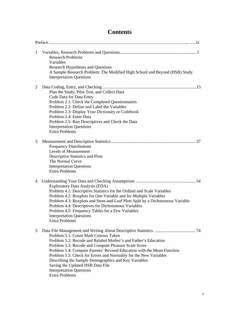
Contents
Preface .................................................................................................................................. …..ix 1 Variables, Research Problems and Questions........................................................................1
Research Problems Variables Research Hypotheses and Questions A Sample Research Problem: The Modified High School and Beyond (HSB) Study Interpretation Questions
2 Data Coding, Entry, and Checking ....................................................................................... 15
Plan the Study, Pilot Test, and Collect Data Code Data for Data Entry
Problem 2.1: Check the Completed Questionnaires Problem 2.2: Define and Label the Variables Problem 2.3: Display Your Dictionary or Codebook Problem 2.4: Enter Data Problem 2.5: Run Descriptives and Check the Data Interpretation Questions Extra Problems
3 Measurement and Descriptive Statistics .............................................................................. 37
Frequency Distributions Levels of Measurement Descriptive Statistics and Plots The Normal Curve Interpretation Questions Extra Problems
4 Understanding Your Data and Checking Assumptions ....................................................... 54
Exploratory Data Analysis (EDA) Problem 4.1: Descriptive Statistics for the Ordinal and Scale Variables Problem 4.2: Boxplots for One Variable and for Multiple Variables Problem 4.3: Boxplots and Stem-and-Leaf Plots Split by a Dichotomous Variable Problem 4.4: Descriptives for Dichotomous Variables Problem 4.5: Frequency Tables for a Few Variables Interpretation Questions Extra Problems
5 Data File Management and Writing About Descriptive Statistics. ..................................... 74
Problem 5.1: Count Math Courses Taken Problem 5.2: Recode and Relabel Mother’s and Father’s Education Problem 5.3: Recode and Compute Pleasure Scale Score Problem 5.4: Compute Parents’ Revised Education with the Mean Function Problem 5.5: Check for Errors and Normality for the New Variables Describing the Sample Demographics and Key Variables Saving the Updated HSB Data File Interpretation Questions
Extra Problems
v
vi CONTENTS
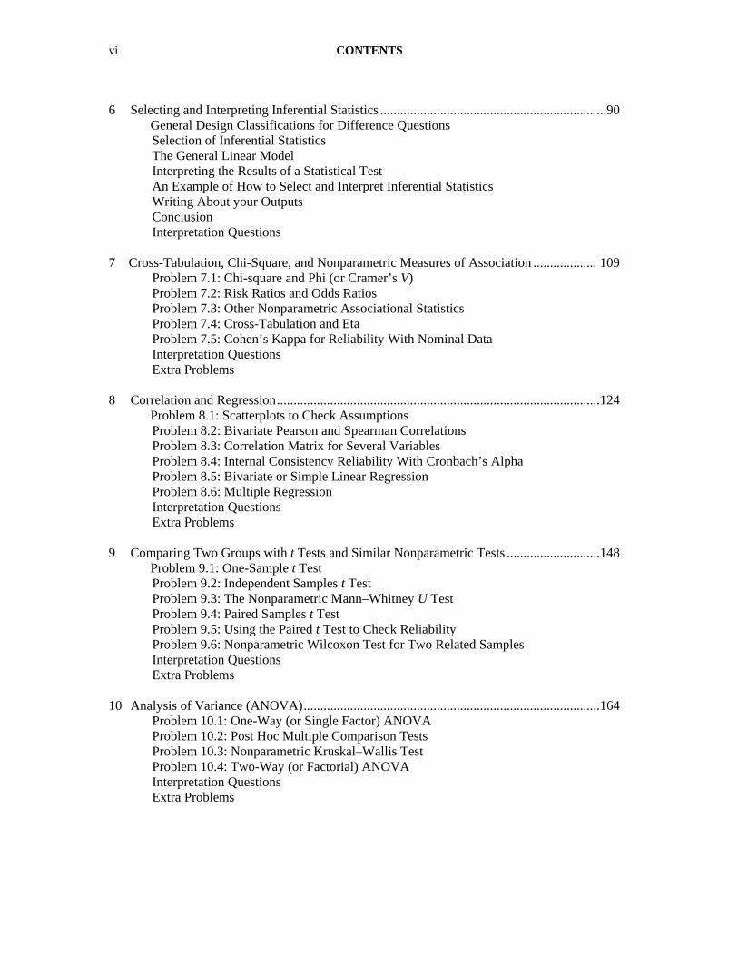
6 Selecting and Interpreting Inferential Statistics .................................................................... 90 General Design Classifications for Difference Questions
Selection of Inferential Statistics The General Linear Model Interpreting the Results of a Statistical Test An Example of How to Select and Interpret Inferential Statistics Writing About your Outputs Conclusion Interpretation Questions
7 Cross-Tabulation, Chi-Square, and Nonparametric Measures of Association ................... 109
Problem 7.1: Chi-square and Phi (or Cramer’s V) Problem 7.2: Risk Ratios and Odds Ratios Problem 7.3: Other Nonparametric Associational Statistics Problem 7.4: Cross-Tabulation and Eta Problem 7.5: Cohen’s Kappa for Reliability With Nominal Data Interpretation Questions Extra Problems
8 Correlation and Regression ................................................................................................. 124 Problem 8.1: Scatterplots to Check Assumptions
Problem 8.2: Bivariate Pearson and Spearman Correlations Problem 8.3: Correlation Matrix for Several Variables Problem 8.4: Internal Consistency Reliability With Cronbach’s Alpha Problem 8.5: Bivariate or Simple Linear Regression Problem 8.6: Multiple Regression Interpretation Questions Extra Problems
9 Comparing Two Groups with t Tests and Similar Nonparametric Tests ............................ 148 Problem 9.1: One-Sample t Test
Problem 9.2: Independent Samples t Test Problem 9.3: The Nonparametric Mann–Whitney U Test Problem 9.4: Paired Samples t Test Problem 9.5: Using the Paired t Test to Check Reliability Problem 9.6: Nonparametric Wilcoxon Test for Two Related Samples Interpretation Questions Extra Problems
10 Analysis of Variance (ANOVA) ......................................................................................... 164
Problem 10.1: One-Way (or Single Factor) ANOVA Problem 10.2: Post Hoc Multiple Comparison Tests Problem 10.3: Nonparametric Kruskal–Wallis Test Problem 10.4: Two-Way (or Factorial) ANOVA Interpretation Questions Extra Problems
CONTENTS vii
Appendices A. Getting Started and Other Useful SPSS Procedures Don Quick & Sophie Nelson ....................................................................................... 185 B. Writing Research Problems and Questions ...................................................................... 195 C. Making Tables and Figures Don Quick…….. ...................................................................................................... 199 D. Answers to Odd Numbered Interpretation Questions ...................................................... 213 For Further Reading ................................................................................................................. 224 Index ........................................................................................................................................ 225
Preface This book is designed to help students learn how to analyze and interpret research. It is intended to be a supplemental text in an introductory (undergraduate or graduate) statistics or research methods course in the behavioral or social sciences or education and it can be used in conjunction with any mainstream text. We have found that this book makes IBM SPSS for Windows easy to use so that it is not necessary to have a formal, instructional computer lab; you should be able to learn how to use the program on your own with this book. Access to the program and some familiarity with Windows is all that is required. Although the program is quite easy to use, there is such a wide variety of options and statistics that knowing which ones to use and how to interpret the printouts can be difficult. This book is intended to help with these challenges. In addition to serving as a supplemental or lab text, this book and its companion Intermediate SPSS book (Leech, Barrett, & Morgan, 4th ed., in press) are useful as reminders to faculty and professionals of the specific steps to take to use SPSS and/or guides to using and interpreting parts of SPSS with which they might be unfamiliar. The Computer Program We used PASW 18 from SPSS, an IBM Company, in this book. Except for enhanced tables and graphics, there are only minor differences among SPSS Versions 10 to 18. In early 2009 SPSS changed the name of its popular Base software package to PASW. Then in October 2009, IBM bought the SPSS Corporation and changed the name of the program used in this book from PASW to IBM SPSS Statistics Base. We expect future Windows versions of this program to be similar so students should be able to use this book with earlier and later versions of the program, which we call SPSS in the text. Our students have used this book, or earlier editions of it, with all of the versions of SPSS; both the procedures and outputs are quite similar. We point out some of the changes at various points in the text. In addition to various SPSS modules that may be available at your university, there are two versions that are available for students, including a 21-day trial period download. The IBM SPSS Statistics Student Version can do all of the statistics in this book. IBM SPSS Statistics GradPack includes the SPSS Base modules as well as advanced statistics, which enable you to do all the statistics in this book plus those in our IBM SPSS for Intermediate Statistics book (Leech, et al., in press) and many others. Goals of This Book Helping you learn how to choose the appropriate statistics, interpret the outputs, and develop skills in writing about the meaning of the results are the main goals of this book. Thus, we have included material on: 1. How the appropriate choice of a statistic is influenced by the design of the research. 2. How to use SPSS to help the researcher answer research questions. 3. How to interpret SPSS outputs. 4. How to write about the outputs in the Results section of a paper. This information will help you develop skills that cover the whole range of the steps in the research process: design, data collection, data entry, data analysis, interpretation of outputs, and writing results. The modified high school and beyond data set (HSB) used in this book is similar to one you might have for a thesis, dissertation, or research project. Therefore, we think it can serve as a model for your analysis. The Web site, http://www.psypress.com/ibm-spss-intro-stats, contains the HSB data file and another data set (called college student data.sav) that is used for the extra statistics problems at the end of each chapter.
ix
x PREFACE
This book demonstrates how to produce a variety of statistics that are usually included in basic statistics courses, plus others (e.g., reliability measures) that are useful for doing research. We try to describe the use and interpretation of these statistics as much as possible in nontechnical, jargon-free language. In part, to make the text more readable, we have chosen not to cite many references in the text; however, we have provided a short bibliography, “For Further Reading,” of some of the books and articles that our students have found useful. We assume that most students will use this book in conjunction with a class that has a textbook; it will help you to read more about each statistic before doing the assignments. Overview of the Chapters Our approach in this book is to present how to use and interpret the SPSS statistics program in the context of proceeding as if the HSB data were the actual data from your research project. However, before starting the assignments, we have three introductory chapters. The first chapter describes research problems, variables, and research questions, and it identifies a number of specific research questions related to the HSB data. The goal is to use this computer program as a tool to help you answer these research questions. (Appendix B provides some guidelines for phrasing or formatting research questions.) Chapter 2 provides an introduction to data coding, entry, and checking with sample questionnaire data designed for those purposes. We developed Chapter 2 because many of you may have little experience with making “messy,” realistic data ready to analyze. Chapter 3 discusses measurement and its relation to the appropriate use of descriptive statistics. This chapter also includes a brief review of descriptive statistics. Chapters 4 and 5 provide you with experience doing exploratory data analysis (EDA), basic descriptive statistics, and data manipulations (e.g., compute and recode) using the high school and beyond (HSB) data set. These chapters are organized in very much the way you might proceed if this were your project. We calculate a variety of descriptive statistics, check certain statistical assumptions, and make a few data transformations. Much of what is done in these two chapters involves preliminary analyses to get ready to answer the research questions that you might state in a report. Chapter 5 ends with examples of how you might write about these descriptive data in a research report or thesis. Chapter 6 provides a brief overview of research designs (e.g., between groups and within subjects). This chapter provides flowcharts and tables useful for selecting an appropriate statistic. Also included is an overview of how to interpret and write about the results of an inferential statistic. This section includes not only testing for statistical significance but also a discussion of effect size measures and guidelines for interpreting them. Chapters 7 through 10 are designed to answer the several research questions posed in Chapter 1 as well as a number of additional questions. Solving the problems in these chapters should give you a good idea of the basic statistics that can be computed with this computer program. Hopefully, seeing how the research questions and design lead naturally to the choice of statistics will become apparent after using this book. In addition, it is our hope that interpreting what you get back from the computer will become more clear after doing these assignments, studying the outputs, answering the interpretation questions, and doing the extra statistics problems. Our Approach to Research Questions, Measurement, and Selection of Statistics In Chapters 1, 3, and 6, our approach is somewhat nontraditional because we have found that students have a great deal of difficulty with some aspects of research and statistics but not others. Most can learn formulas and “crunch” the numbers quite easily and accurately with a calculator or with a computer. However, many have trouble knowing what statistics to use and how to
IBM SPSS FOR INTRODUCTORY STATISTICS xi
interpret the results. They do not seem to have a “big picture” or see how research design and measurement influence data analysis. Part of the problem is inconsistent terminology. We are reminded of Bruce Thompson’s frequently repeated, intentionally facetious remark at his many national workshops: “We use these different terms to confuse the graduate students.” For these reasons, we have tried to present a semantically consistent and coherent picture of how research design leads to three basic kinds of research questions (difference, associational, and descriptive) that, in turn, lead to three kinds or groups of statistics with the same names. We realize that these and other attempts to develop and utilize a consistent framework are both nontraditional and somewhat of an oversimplification. However, we think the framework and consistency pay off in terms of student understanding and ability to actually use statistics to help answer their research questions. Instructors who are not persuaded that this framework is useful can skip Chapters 1, 3, and 6 and still have a book that helps their students use and interpret SPSS. Major Changes in This Edition The major change in this edition is updating the windows and text to SPSS/PASW 18. We have also attempted to correct any typos in the 3rd edition and clarify some passages. We expanded the appendix about Getting Started with SPSS (Appendix A) to include several useful procedures that were not discussed in the body of the text. We have expanded the discussion of effect size measures to include information on risk and odds ratios in Chapter 7. As noted earlier, Chapter 5 has been expanded to include how to write about descriptive statistics. In addition, we have modified the format of the write-up examples to meet the new changes in APA format in the 6th edition (2010) of the Publication Manual. Although this edition was written using version 18, the program is sufficiently similar to prior versions of this software that we feel you should be able to use this book with earlier and later versions as well. Instructional Features Several user friendly features of this book include: 1. Both words and the key windows that you see when performing the statistical analyses. This
has been helpful to “visual learners.” 2. The complete outputs for the analyses that we have done so you can see what you will get
(we have done some editing in SPSS to make the outputs fit better on the pages). 3. Callout boxes on the outputs that point out parts of the output to focus on and indicate what
they mean. 4. For each output, a boxed interpretation section that will help you understand the output. 5. Chapter 6 provides specially developed flowcharts and tables to help you select an
appropriate inferential statistic and interpret statistical significance and effect sizes. This chapter also provides an extended example of how to identify and write a research problem, research questions, and a results paragraph.
6. For the inferential statistics in Chapters 7–10, an example of how to write about the output and make a table for a thesis, dissertation, or research paper.
7. Interpretation questions for each chapter that stimulate you to think about the information in the chapter.
8. Several Extra Problems at the end of each chapter for you to run with the program. 9. Appendix A provides information about how to get started with SPSS and how to use several
commands not discussed in the chapters. 10. Appendix B provides examples of how to write research problems and
questions/hypotheses; Appendix C shows how to make tables and figures. 11. Answers to the odd numbered interpretation questions are provided in Appendix D. 12. Two data sets on a student resource site. These realistic data sets provide you with data to
be used to solve the chapter problems and the Extra Problems using SPSS.
xii PREFACE
13. An Instructor Resource Web site is available to course instructors who request access from the publisher. To request access, please visit the book page or the Textbook Resource tabs at www.psypress.com. It contains aids for teaching the course, including PowerPoint slides, the answers to the even numbered interpretation questions, and information related to the even numbered Extra Problems. Researchers who purchase copies for their personal use can access the data files by visiting www.psypress.com/ibm-spss-intro-stats.
Major Statistical Features of This Edition Based on our experiences using the book with students, feedback from reviewers and other users, and the revisions in policy and best practice specified by the APA Task Force on Statistical Inference (1999) and the 6th Edition of the APA Publication Manual (2010), we have included discussions of: 1. Effect size. We discuss effect size in each interpretation section to be consistent with the
requirements of the revised APA manual. Because this program doesn’t provide effect sizes for all the demonstrated statistics, we often have to show how to estimate or compute them by hand.
2. Writing about outputs. We include examples of how to write about and make APA type tables from the information in the outputs. We have found the step from interpretation to writing quite difficult for students so we put emphasis on writing research results.
3. Data entry and checking. Chapter 2 on data entry, variable labeling, and data checking is based on a small data set developed for this book. What is special about this is that the data are displayed as if they were on copies of actual questionnaires answered by participants. We built in problematic responses that require the researcher or data entry person to look for errors or inconsistencies and to make decisions. We hope this quite realistic task will help students be more sensitive to issues of data checking before doing analyses.
4. Descriptive statistics and testing assumptions. In Chapters 4 and 5 we emphasize exploratory data analysis (EDA), how to test assumptions, and data file management.
5. Assumptions. When each inferential statistic is introduced in Chapters 7–10, we have a brief section about its assumptions and when it is appropriate to select that statistic for the problem or question at hand.
6. All the basic descriptive and inferential statistics such as chi-square, correlation, t tests, and one-way ANOVA covered in basic statistics books. Our companion book, Leech, et al., 4th ed. (in press), IBM SPSS for Intermediate Statistics: Use and Interpretation, also published by Routledge/Taylor & Francis, is on the “For Further Reading” list at the end of this book. We think that you will find it useful if you need more complete examples and interpretations of complex statistics including but not limited to Cronbach’s alpha, multiple regression, and factorial ANOVA that are introduced briefly in this book.
7. Reliability assessment. We present some ways of assessing reliability in the cross-tabulation, correlation, and t test chapters of this book. More emphasis on reliability and testing assumptions is consistent with our strategy of presenting computer analyses that students would use in an actual research project.
8. Nonparametric statistics. We include the nonparametric tests that are similar to the t tests (Mann–Whitney and Wilcoxon) and single factor ANOVA (Kruskal–Wallis) in appropriate chapters as well as several nonparametric measures of association. This is consistent with the emphasis on checking assumptions because it provides alternative procedures for the student when key assumptions are markedly violated.
9. SPSS syntax. We show the syntax along with the outputs because a number of professors and skilled students like seeing and prefer using syntax to produce outputs. How to include SPSS syntax in the output and to save and reuse it is presented in Appendix A. Use of syntax to
IBM SPSS FOR INTRODUCTORY STATISTICS xiii
write commands not otherwise available in SPSS is presented briefly in our companion volume, Leech et al. (in press).
Bullets, Arrows, Bold, and Italics To help you do the problems, we have developed some conventions. We use bullets to indicate actions in SPSS windows that you will take. For example: • Highlight gender and math achievement. • Click on the arrow to move the variables into the right-hand box. • Click on Options to get Fig. 2.16. • Check Mean, Std Deviation, Minimum, and Maximum. • Click on Continue. Note that the words in italics are variable names and words in bold are words that you will see in the windows and utilize to produce the desired output. In the text they are spelled and capitalized as you see them in the windows. Bold is also used to identify key terms when they are introduced, defined, or important to understanding. To access a window from what SPSS calls the Data View (see Chapter 2), the words you will see in the pull down menus are given in bold with arrows between them. For example: • Select Analyze → Descriptive Statistics → Frequencies. (This means pull down the Analyze menu, then slide your cursor down to Descriptive Statistics and over to Frequencies, and click.) Occasionally, we have used underlines to emphasize critical points or commands. We have tried hard to make this book accurate and clear so that it could be used by students and professionals to learn to compute and interpret statistics without the benefit of a class. However, we find that there are always some errors and places that are not totally clear. Thus, we would like for you to help us identify any grammatical or statistical errors and to point out places that need to be clarified. Please send suggestions to [email protected].
Acknowledgments
This SPSS/PASW book is consistent with and could be used as a supplement for Gliner, Morgan, and Leech (2009), Research Methods in Applied Settings: An Integrated Approach to Design and Analysis (2nd ed.), which provides extended discussions of how to conduct a quantitative research project as well as understand the key concepts. Or this SPSS book could be a supplement for Morgan, Gliner, and Harmon (2006), Understanding and Evaluating Research in Applied and Clinical Settings, which is a shorter book emphasizing reading and evaluating research articles and statistics. Information about both books can be found at www.psypress.com. Because this book draws heavily on these two research methods texts and on earlier editions of this book, we need to acknowledge the important contribution of three current and former colleagues. We thank Jeff Gliner for allowing us to use material in Chapters 1, 3, and 6. Bob Harmon facilitated much of our effort to make statistics and research methods understandable to students, clinicians, and other professionals. We hope this book will serve as a memorial to him and the work he supported. Orlando Griego was a co-author of the first edition of this SPSS book; it still shows the imprint of his student-friendly writing style.
xiv PREFACE
We would like to acknowledge the assistance of the many students who have used earlier versions of this book and provided helpful suggestions for improvement. We could not have completed the task or made it look so good without our technology consultants, Don Quick and Ian Gordon, and our word processor, Sophie Nelson. Linda White, Catherine Lamana, and Alana Stewart and several other student workers were key to making figures in earlier versions. Jikyeong Kang, Bill Sears, LaVon Blaesi, Mei-Huei Tsay, and Sheridan Green assisted with classes and the development of materials for the DOS and earlier Windows versions of the assignments. Lisa Vogel, Don Quick, Andrea Weinberg, Pam Cress, Joan Clay, Laura Jensen James Lyall, Joan Anderson, and Yasmine Andrews wrote or edited parts of earlier editions. We thank Don Quick and Sophie Nelson for writing appendixes for this edition. Jeff Gliner, Jerry Vaske, Jim zumBrunnen, Laura Goodwin, James Benedict, Barry Cohen, John Ruscio, Tim Urdan, and Steve Knotek provided reviews and suggestions for improving the text. Bob Fetch and Ray Yang provided helpful feedback on the readability and user friendliness of the text. Finally, the patience of our spouses (Hildy, Grant, Susan, and Terry) and families enabled us to complete the task without too much family strain.
15
CHAPTER 2
Data Coding, Entry, and Checking
This chapter begins with a very brief overview of the initial steps in a research project. After this
introduction, the chapter focuses on: (a) getting your data ready to enter into the data editor or a
spreadsheet, (b) defining and labeling variables, (c) entering the data appropriately, and (d)
checking to be sure that data entry was done correctly without errors.
Plan the Study, Pilot Test, and Collect Data
Plan the study. As discussed in Chapter 1, the research starts with identification of a research
problem and research questions or hypotheses. It is also necessary to plan the research design
before you select the data collection instrument(s) and begin to collect data. Most research
methods books discuss this part of the research process extensively (e.g., see Gliner, Morgan, &
Leech, 2009).
Select or develop the instrument(s). If there is an appropriate, available instrument that provides
reliable and valid data and it has been used with a population similar to yours, it is usually
desirable to use it. However, sometimes it is necessary to modify an existing instrument or
develop your own. For this chapter, we have developed a short questionnaire to be given to
students at the end of a course. Remember that questionnaires or surveys are only one way to
collect quantitative data. You could also use structured interviews, observations, tests,
standardized inventories, or some other type of data collection method. Research methods and
measurement books have one or more chapters devoted to the selection and development of data
collection instruments. A useful book on the development of questionnaires is Fink (2009).
Pilot test and refine instruments. It is always desirable to try out your instrument and directions
with, at the very least, a few colleagues or friends. When possible, you also should conduct a
pilot study with a sample similar to the one you plan to use later. This is especially important if
you developed the instrument or if it is going to be used with a population different from the
one(s) for which it was developed and on which it was previously used.
Pilot participants should be asked about the clarity of the items and whether they think any items
should be added or deleted. Then, use the feedback to make modifications in the instrument
before beginning the actual data collection. If the instrument is changed, the pilot data should not
be added to the data collected for the study. Content validity can also be checked by asking
experts to judge whether your items cover all aspects of the domain you intended to measure and
whether they are in appropriate proportions relative to that domain.
Collect the data. The next step in the research process is to collect the data. There are several
ways to collect questionnaire or survey data (such as telephone, mail, or e-mail). We do not
discuss them here because that is not the purpose of this book. The Fink (2009) book, How to
Conduct Surveys: A Step by Step Guide, provides information on the various methods for
collecting survey data.
You should Ucheck your raw dataU after you collect it even Ubefore it is enteredU into the computer.
Make sure that the participants marked their score sheets or questionnaires appropriately; check
16 CHAPTER 2
to see if there are double answers to a question (when only one is expected) or answers that are
marked between two rating points. If this happens, you need to have a rule (e.g., ―use the
average‖) that you can apply consistently. Thus, you should ―clean up‖ your data, making sure
they are clear, consistent, and readable, before entering them into a data file.
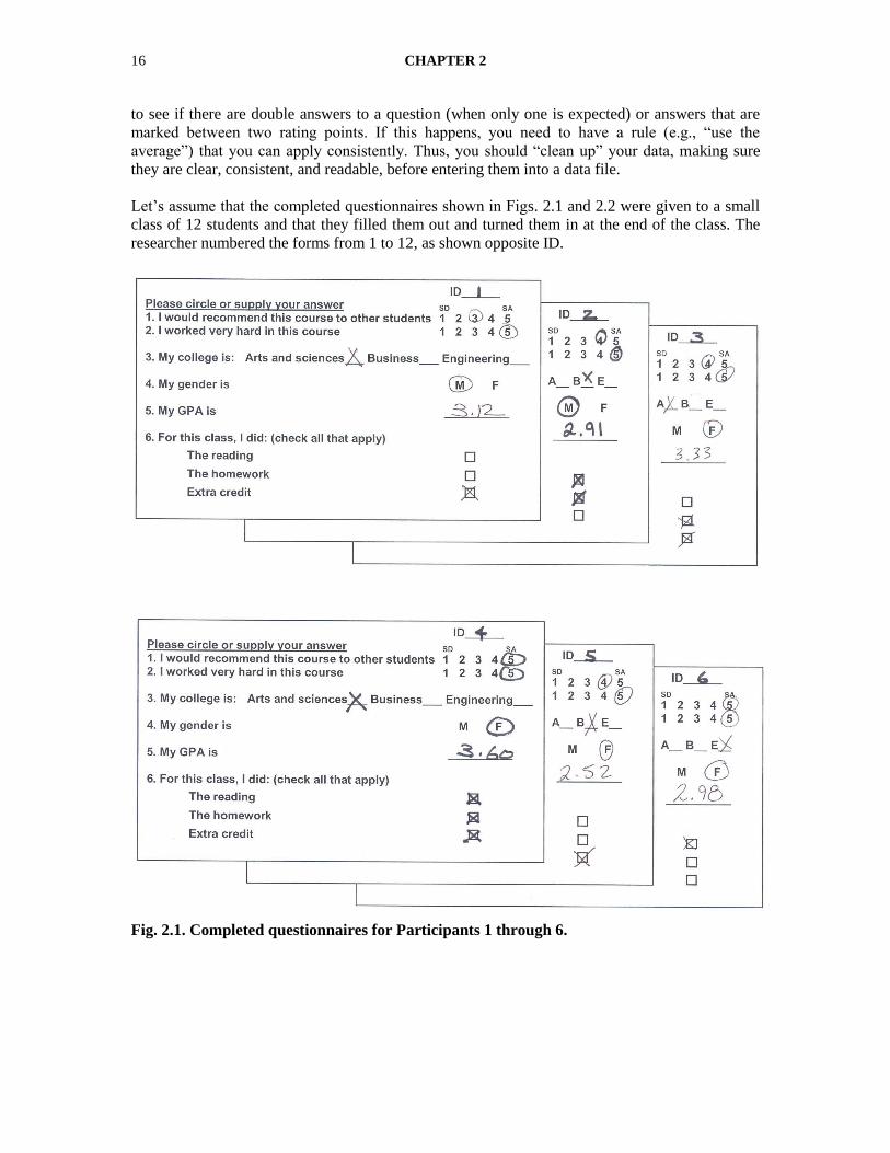
Let’s assume that the completed questionnaires shown in Figs. 2.1 and 2.2 were given to a small
class of 12 students and that they filled them out and turned them in at the end of the class. The
researcher numbered the forms from 1 to 12, as shown opposite ID.
Fig. 2.1. Completed questionnaires for Participants 1 through 6.
DATA CODING, ENTRY, AND CHECKING 17
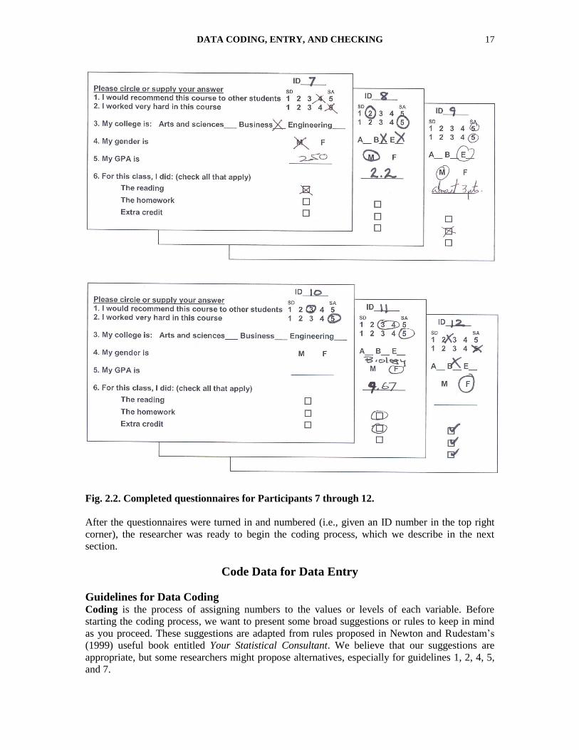
Fig. 2.2. Completed questionnaires for Participants 7 through 12.
After the questionnaires were turned in and numbered (i.e., given an ID number in the top right
corner), the researcher was ready to begin the coding process, which we describe in the next
section.
Code Data for Data Entry
Guidelines for Data Coding Coding is the process of assigning numbers to the values or levels of each variable. Before
starting the coding process, we want to present some broad suggestions or rules to keep in mind
as you proceed. These suggestions are adapted from rules proposed in Newton and Rudestam’s
(1999) useful book entitled Your Statistical Consultant. We believe that our suggestions are
appropriate, but some researchers might propose alternatives, especially for guidelines 1, 2, 4, 5,
and 7.
18 CHAPTER 2
1. All data should be numeric. Even though it is possible to use letters or words (string
variables) as data, it is not desirable to do so. For example, we could code gender as M for
male and F for female, but in order to do most statistics you would have to convert the letters
or words to numbers. It is easier to do this conversion before entering the data into the
computer as we have done with the HSB data set (see Fig. 1.3). You will see in Fig. 2.3 that we
decided to code females as 1 and males as 0. This is called dummy coding. In essence, the 0
means ―not female.‖ Dummy coding is useful if you will want to use the data in some types of
analyses and for obtaining descriptive statistics. For example, the mean of data coded this way
will tell you the percentage of participants who fall in the category coded as ―1.‖ We could, of
course, code males as 1 and females as 0, or we could code one gender as 1 and the other as 2.
However, it is crucial that you be consistent in your coding (e.g., for this study, all males are
coded 0 and females 1) and that you have a way to remind yourself and others of how you did
the coding. Later in this chapter, we show how you can provide such a record, called a
codebook or dictionary.
2. Each variable for each case or participant must occupy the same column in the Data
Editor. It is important that data from each participant occupy only one line (row), and each
column must contain data on the same variable for all the participants. The data editor, into
which you will enter data, facilitates this by putting the short variable names that you choose at
the top of each column, as you saw in Chapter 1, Fig. 1.3. If a variable is measured more than
once (e.g., pretest and posttest), it will be entered in two columns with somewhat different
names, such as mathpre and mathpost.
3. All values (codes) for a variable must be mutually exclusive. That is, only one value or
number can be recorded for each variable. Some items, like our item 6 in Fig. 2.3, allow for
participants to check more than one response. In that case, the item should be divided into a
separate variable for each possible response choice, with one value of each variable (usually 1)
corresponding to yes (i.e., checked) and the other to no (usually 0, for not checked). For
example, item 6 becomes variables 6, 7, and 8 (see Fig. 2.3). Items should be phrased so that
persons would logically choose only one of the provided options, and all possible options
should be provided. A final category labeled ―other‖ may be provided in cases where all
possible options cannot be listed, but these ―other‖ responses are usually quite diverse and thus
may not be very useful for statistical purposes.
4. Each variable should be coded to obtain maximum information. Do not collapse categories
or values when you set up the codes for them. If needed, let the computer do it later. In general,
it is desirable to code and enter data in as detailed a form as available. Thus, enter actual test
scores, ages, GPAs, and so forth, if you know them. It is good practice to ask participants to
provide information that is quite specific. However, you should be careful not to ask questions
that are so specific that the respondent may not know the answer or may not feel comfortable
providing it. For example, you will obtain more information by asking participants to state their
GPA to two decimals (as in Figs. 2.1 and 2.2) than if you asked them to select from a few
broad categories (e.g., less than 2.0, 2.0–2.49, 2.50–2.99, etc). However, if students don’t know
their GPA or don’t want to reveal it precisely, they may leave the question blank or write in a
difficult to interpret answer, as discussed later.
These issues might lead you to provide a number of categories, each with a relatively narrow
range of values, for variables such as age, weight, and income. Never collapse such categories
before you enter the data into the data editor. For example, if you have age categories for
university undergraduates 16–17, 18–20, 21–23, and so forth, and you realize that there are
DATA CODING, ENTRY, AND CHECKING 19
only a few students younger than 18, keep the codes as is for now. ULaterU you can make a new
category of 20 or younger by using a function, Transform => Recode. If you collapse
categories before you enter the data, the extra information will no longer be available.
5. For each participant, there must be a code or value for each variable. These codes should
be numbers, except for variables for which the data are missing. We recommend using blanks
when data are missing or unusable because Uthis program is designed to handle blanks as
missing valuesU. However, sometimes you may have more than one type of missing data, such
as items left blank and those that had an answer that was not appropriate or usable. In this case
you may assign numeric codes such as 98 and 99 to them, but you Umust tell the program that
these codes are for missing valuesU, or it will treat them as actual data.
6. Apply any coding rules consistently for all participants. This means that if you decide to
treat a certain type of response as, say, missing for one person, you must do the same for all
other participants.
7. Use high numbers (values or codes) for the “agree,” “good,” or “positive” end of a
variable that is ordered. Sometimes you will see questionnaires that use 1 for ―strongly
agree,‖ and 5 for ―strongly disagree.‖ This is not wrong as long as you are clear and consistent.
However, you are less likely to get confused when interpreting your results if high values have
a positive meaning.
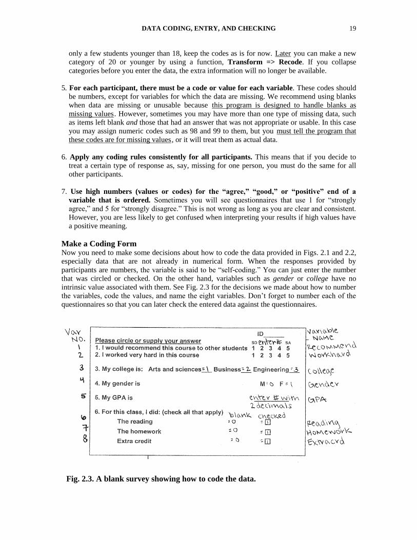
Make a Coding Form Now you need to make some decisions about how to code the data provided in Figs. 2.1 and 2.2,
especially data that are not already in numerical form. When the responses provided by
participants are numbers, the variable is said to be ―self-coding.‖ You can just enter the number
that was circled or checked. On the other hand, variables such as gender or college have no
intrinsic value associated with them. See Fig. 2.3 for the decisions we made about how to number
the variables, code the values, and name the eight variables. Don’t forget to number each of the
questionnaires so that you can later check the entered data against the questionnaires.
Fig. 2.3. A blank survey showing how to code the data.
20 CHAPTER 2
Problem 2.1: Check the Completed Questionnaires
Now examine Figs. 2.1 and 2.2 for incomplete, unclear, or double answers. Stop and do this now,
before proceeding. What issues did you see? The researcher needs to make rules about how to
handle these problems and note them on the questionnaires or on a master ―coding instructions‖
sheet so that the same rules are used for all cases.
We have identified at least 11 responses on 6 of the 12 questionnaires that need to be clarified.
Can you find them all? How would you resolve them? UWrite on Figs. 2.1 and 2.2 how you would
handle each issueU that you see.
Make Rules About How to Handle These Problems For each type of incomplete, blank, unclear, or double answer, you need to make a rule for what
to do. As much as possible, you should make these rules before data collection, but there may
well be some unanticipated issues. It is important that you apply the rules consistently for all
similar problems so as not to bias your results.
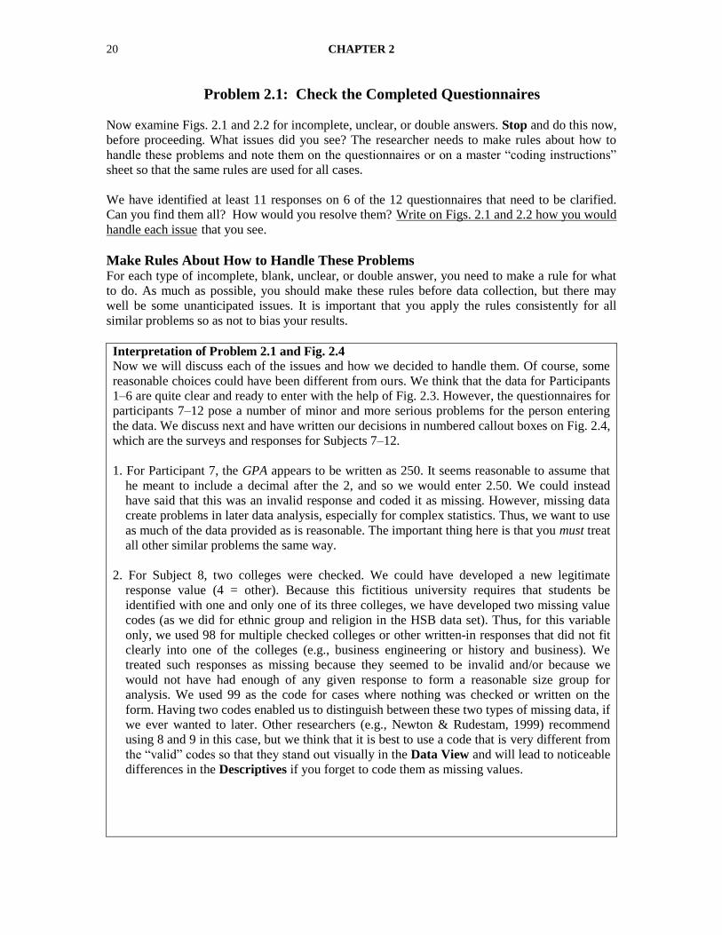
Interpretation of Problem 2.1 and Fig. 2.4
Now we will discuss each of the issues and how we decided to handle them. Of course, some
reasonable choices could have been different from ours. We think that the data for Participants
1–6 are quite clear and ready to enter with the help of Fig. 2.3. However, the questionnaires for
participants 7–12 pose a number of minor and more serious problems for the person entering
the data. We discuss next and have written our decisions in numbered callout boxes on Fig. 2.4,
which are the surveys and responses for Subjects 7–12.
1. For Participant 7, the GPA appears to be written as 250. It seems reasonable to assume that
he meant to include a decimal after the 2, and so we would enter 2.50. We could instead
have said that this was an invalid response and coded it as missing. However, missing data
create problems in later data analysis, especially for complex statistics. Thus, we want to use
as much of the data provided as is reasonable. The important thing here is that you must treat
all other similar problems the same way.
2. For Subject 8, two colleges were checked. We could have developed a new legitimate
response value (4 = other). Because this fictitious university requires that students be
identified with one and only one of its three colleges, we have developed two missing value
codes (as we did for ethnic group and religion in the HSB data set). Thus, for this variable
only, we used 98 for multiple checked colleges or other written-in responses that did not fit
clearly into one of the colleges (e.g., business engineering or history and business). We
treated such responses as missing because they seemed to be invalid and/or because we
would not have had enough of any given response to form a reasonable size group for
analysis. We used 99 as the code for cases where nothing was checked or written on the
form. Having two codes enabled us to distinguish between these two types of missing data, if
we ever wanted to later. Other researchers (e.g., Newton & Rudestam, 1999) recommend
using 8 and 9 in this case, but we think that it is best to use a code that is very different from
the ―valid‖ codes so that they stand out visually in the Data View and will lead to noticeable
differences in the Descriptives if you forget to code them as missing values.
DATA CODING, ENTRY, AND CHECKING 21
3. Also, Subject 8 wrote 2.2 for his GPA. It seems reasonable to enter 2.20 as the GPA.
Actually, in this case, if we enter 2.2, the program will treat it as 2.20 because we will tell it
to use two decimal places for this variable.
4. We decided to enter 3.00 for Participant 9’s GPA. Of course, the actual GPA could be higher
or, more likely, lower, but 3.00 seems to be the best choice given the information provided
by the student (i.e., ―about 3 pt‖).
5. Participant 10 only answered the first two questions, so there were lots of missing data. It
appears that he or she decided not to complete the questionnaire. We made a rule that if three
out of the first five items were blank or invalid, we would throw out that whole questionnaire
as invalid. In your research report, you should state how many questionnaires were thrown
out and for what reason(s). Usually you would not enter any data from that questionnaire, so
you would only have 11 subjects or cases to enter. To show you how you would code
someone’s college if they left it blank, we did not delete this subject at this time.
6. For Subject 11, there are several problems. First, she circled both 3 and 4 for the first item; a
reasonable decision is to enter the average or midpoint, 3.50.
7. Participant 11 has written in ―biology‖ for college. Although there is no biology college at
this university, it seems reasonable to enter 1 = arts and sciences in this case and in other
cases (e.g., history = 1, marketing = 2, civil = 3) where the actual college is clear. See the
discussion of Issue 2 for how to handle unclear examples.
8. Participant 11 also entered 9.67 for the GPA, which is an invalid response because this
university has a 4-point grading system (4.00 is the maximum possible GPA). To show you
one method of checking the entered data for errors, we will go ahead and enter 9.67. If you
examine the completed questionnaires carefully, you should be able to spot errors like this in
the data and enter a blank for missing/invalid data.
9. Enter 1 for reading and homework for Participant 11 (even though they were circled rather
than checked). Also enter 0 for extra credit (not checked) as you would for all the boxes left
unchecked by other participants (except Subject 10, who, as stated in number 5 above, did
not complete the questionnaire). Even though this person circled the boxes rather than
putting X’s or checks in them, her intent is clear.
10. As in Point 6, we decided to enter 2.5 for Participant 12’s X between 2 and 3.
11. Participant 12 also left GPA blank so, using the general (system) missing value code, we
left it blank.
22 CHAPTER 2
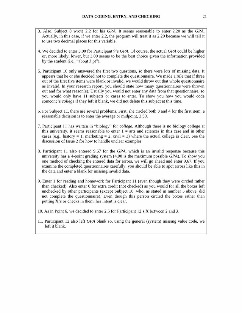
Fig. 2.4. Completed survey with callout boxes showing how we handled problem responses.
5. Leave all variables
blank, except enter 99,
missing, for college.
1. Enter 2.50. 3. Enter 2.20.
2. Enter 98.
4. Enter 3.00.
6. Enter 3.5.
7. Enter 1.
8. For now enter 9.67, but see
accompanying discussion.
9. Enter 1 for
reading and
homework.
11.
Leave
blank,
missing
.
10. Enter 2.5.
DATA CODING, ENTRY, AND CHECKING 23
Clean up Completed Questionnaires Now that you have made your rules and decided how to handle each problem, you need to make
these rules clear to whoever will enter the data. As mentioned earlier, we put our decisions in
callout boxes on Fig. 2.4; a common procedure would be to write your decisions on the
questionnaires, perhaps in a different color.
2BProblem 2.2: Define and Label the Variables
The next step is to create a data file into which you will enter the data. If you do not have the
program open, you need to log on. When you see the startup window, click the Type in data
button; then you should see a blank Data Editor that will look something like Fig. 2.5. Also be
sure that Display Commands in the Log is checked (see Appendix A). You should also examine
Appendix A if you need more help getting started.
This section helps you name and label the variables. In the next section, we show you how to
enter data. First, let’s define and label the first two variables, which are two 5-point Likert ratings.
To do this we need to use the Variable View screen. Look at the bottom left corner of the Data
Editor to see whether you are in the Data View or Variable View screen by noting which tab is
white. If you are in Data View, to get to Variable View do the following:
Click on the Variable View tab at the bottom left of your screen. This will bring up a screen
similar to Fig. 2.5. (Or, double click on var above the blank column to the far left side of the
Data View.)
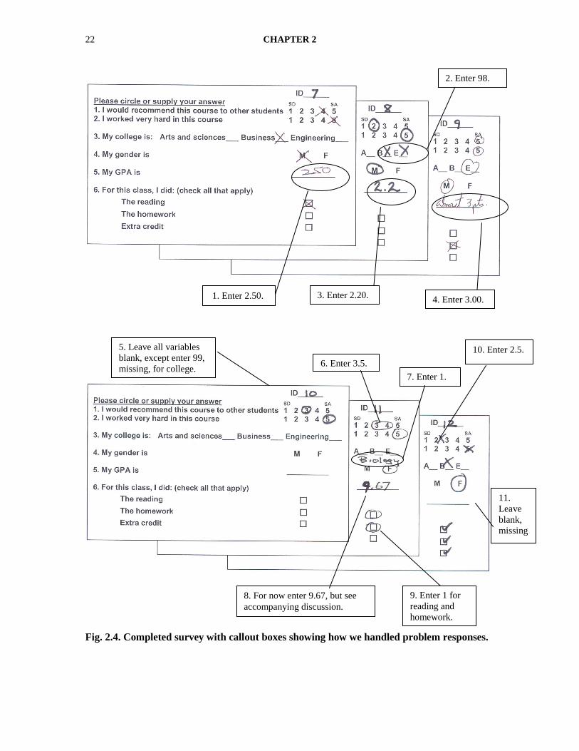
In this window, you will see 11 columns that will allow you to input the variable name, type of
variable, width, number of decimals, variable label, value labels, missing values other than
blanks, columns, align data left or right, measurement type, and variable role.
Define and Label Two Likert-Type Variables We now begin to enter information to name, label, and define the characteristics of the variables
used in this chapter.
Click in the blank box directly under Name in Fig. 2.5.
Type recommend in this box. Notice the number 1 to the left of this box. This indicates that
you are entering your first variable.F
1F
Press enter. This will insert the program’s default values for variables. You need to check to
be sure these are correct for each of your variables and make changes if needed.
1 It is no longer necessary to keep variable names at eight characters or less, but short names are desirable.
Other rules about variable names still apply (see footnote 5 in Chapter 1). Note also that in this book we use
bullets to indicate instructions about SPSS actions (e.g., click, highlight), and we use bold for key terms
displayed in SPSS windows (e.g., Name).
Fig. 2.5. Blank variable view screen in the data editor.
24 CHAPTER 2
Note that the Type is numeric, Width = 8, Decimals = 2, Label = (blank), Values = None,
Missing = None, Columns = 8, Align = right, Measure = scale, Role = input.
For this assignment, we will keep the default values for Type, Width, Columns, and Align. On
the Variable View screen, you will notice that the default for Type is Numeric. This refers to the
type of variable you are entering. Usually, you will only use the Numeric option. Numeric means
the data are numbers. String would be used if you input words or letters such as ―M‖ for males
and ―F‖ for females. However, it is best not to enter words or letters because you wouldn’t be
able to do many statistics without recoding them as numbers. In this book, Uwe will always keep
the Type as Numeric.U
We recommend keeping the Width at eight, and keeping the Columns at eight. We will always
Align the numbers to the right. Sometimes, we will change the settings for the other columns.
Now let’s continue with defining and labeling the recommend variable.
For this variable, leave the decimals at 2.
Click on the box under ―Label‖ and type I recommend course in the Label box. This longer
label will show in appropriate windows and on your printouts. The labels can be up to 40
characters Ubut it is best to keep them about 20 or less Uor your outputs may be difficult to read.
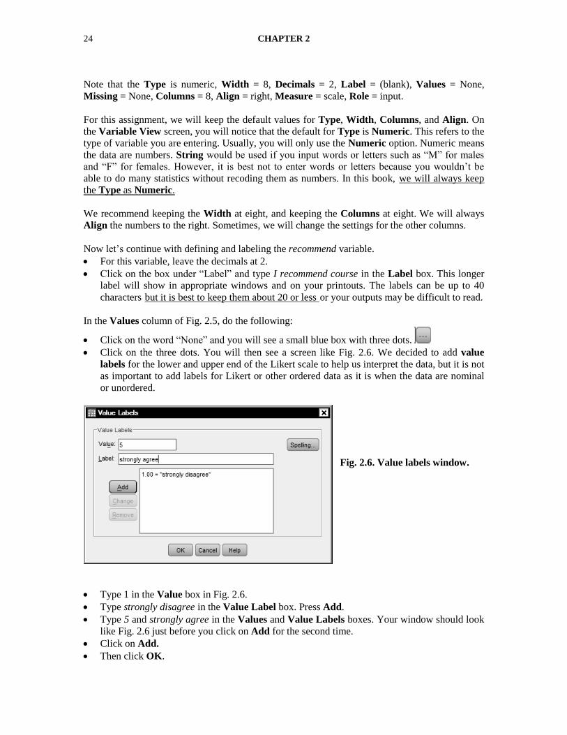
In the Values column of Fig. 2.5, do the following:
Click on the word ―None‖ and you will see a small blue box with three dots.
Click on the three dots. You will then see a screen like Fig. 2.6. We decided to add value
labels for the lower and upper end of the Likert scale to help us interpret the data, but it is not
as important to add labels for Likert or other ordered data as it is when the data are nominal
or unordered.
Type 1 in the Value box in Fig. 2.6.
Type strongly disagree in the Value Label box. Press Add.
Type 5 and strongly agree in the Values and Value Labels boxes. Your window should look
like Fig. 2.6 just before you click on Add for the second time.
Click on Add.
Then click OK.
Fig. 2.6. Value labels window.
DATA CODING, ENTRY, AND CHECKING 25
Leave the cells for the Missing to Measure columns in Fig. 2.5 as they currently appear.
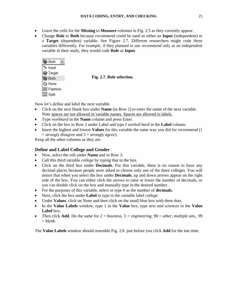
Change Role to Both because recommend could be used as either an Input (independent) or
a Target (dependent) variable. See Figure 2.7. Different researchers might code these
variables differently. For example, if they planned to use recommend only as an independent
variable in their study, they would code Role as Input.
Now let’s define and label the next variable.
Click on the next blank box under Name (in Row 2) to enter the name of the next variable.
Note Uspaces are not allowed in variable names. Spaces are allowed in labels. U
Type workhard in the Name column and press Enter.
Click on the box in Row 2 under Label and type I worked hard in the Label column.
Insert the highest and lowest Values for this variable the same way you did for recommend (1
= strongly disagree and 5 = strongly agree).
Keep all the other columns as they are.
Define and Label College and Gender
Now, select the cell under Name and in Row 3.
Call this third variable college by typing that in the box.
Click on the third box under Decimals. For this variable, there is no reason to have any
decimal places because people were asked to choose only one of the three colleges. You will
notice that when you select the box under Decimals, up and down arrows appear on the right
side of the box. You can either click the arrows to raise or lower the number of decimals, or
you can double click on the box and manually type in the desired number.
For the purposes of this variable, select or type 0 as the number of decimals.
Next, click the box under Label to type in the variable label college.
Under Values, click on None and then click on the small blue box with three dots.
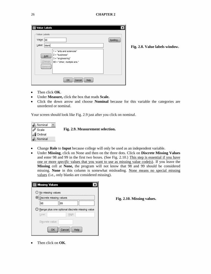
In the Value Labels window, type 1 in the Value box, type arts and sciences in the Value
Label box.
Then click Add. Do the same for 2 = business, 3 = engineering, 98 = other, multiple ans., 99
= blank.
The Value Labels window should resemble Fig. 2.8 just before you click Add for the last time.
Fig. 2.7. Role selection.
26 CHAPTER 2
Then click OK.
Under Measure, click the box that reads Scale.
Click the down arrow and choose Nominal because for this variable the categories are
unordered or nominal.
Your screen should look like Fig. 2.9 just after you click on nominal.
Change Role to Input because college will only be used as an independent variable.
Under Missing, click on None and then on the three dots. Click on Discrete Missing Values
and enter 98 and 99 in the first two boxes. (See Fig. 2.10.) UThis step is essential if you have
one or more specific values that you want to use as missing value code(s)U. If you leave the
Missing cell at None, the program will not know that 98 and 99 should be considered
missing. None in this column is somewhat misleading. UNone means no special missing
valuesU (i.e., only blanks are considered missing).
Then click on OK.
Fig. 2.10. Missing values.
Fig. 2.8. Value labels window.
Fig. 2.9. Measurement selection.
DATA CODING, ENTRY, AND CHECKING 27
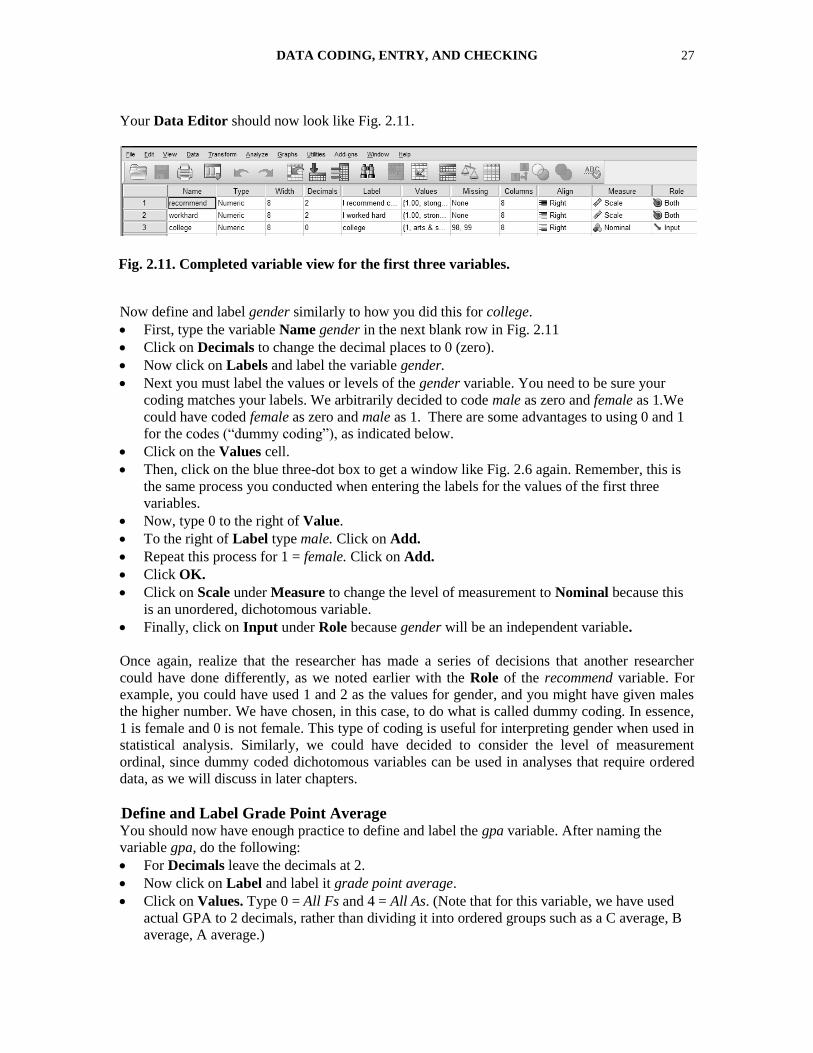
Your Data Editor should now look like Fig. 2.11.
Now define and label gender similarly to how you did this for college.
First, type the variable Name gender in the next blank row in Fig. 2.11
Click on Decimals to change the decimal places to 0 (zero).
Now click on Labels and label the variable gender.
Next you must label the values or levels of the gender variable. You need to be sure your
coding matches your labels. We arbitrarily decided to code male as zero and female as 1.We
could have coded female as zero and male as 1. There are some advantages to using 0 and 1
for the codes (―dummy coding‖), as indicated below.
Click on the Values cell.
Then, click on the blue three-dot box to get a window like Fig. 2.6 again. Remember, this is
the same process you conducted when entering the labels for the values of the first three
variables.
Now, type 0 to the right of Value.
To the right of Label type male. Click on Add.
Repeat this process for 1 = female. Click on Add.
Click OK.
Click on Scale under Measure to change the level of measurement to Nominal because this
is an unordered, dichotomous variable.
Finally, click on Input under Role because gender will be an independent variable.
Once again, realize that the researcher has made a series of decisions that another researcher
could have done differently, as we noted earlier with the Role of the recommend variable. For
example, you could have used 1 and 2 as the values for gender, and you might have given males
the higher number. We have chosen, in this case, to do what is called dummy coding. In essence,
1 is female and 0 is not female. This type of coding is useful for interpreting gender when used in
statistical analysis. Similarly, we could have decided to consider the level of measurement
ordinal, since dummy coded dichotomous variables can be used in analyses that require ordered
data, as we will discuss in later chapters.
4BDefine and Label Grade Point Average You should now have enough practice to define and label the gpa variable. After naming the
variable gpa, do the following:
For Decimals leave the decimals at 2.
Now click on Label and label it grade point average.
Click on Values. Type 0 = All Fs and 4 = All As. (Note that for this variable, we have used
actual GPA to 2 decimals, rather than dividing it into ordered groups such as a C average, B
average, A average.)
Fig. 2.11. Completed variable view for the first three variables.
28 CHAPTER 2
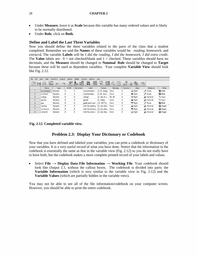
Under Measure, leave it as Scale because this variable has many ordered values and is likely
to be normally distributed.
Under Role, click on Both.
3BDefine and Label the Last Three Variables Now you should define the three variables related to the parts of the class that a student
completed. Remember we said the Names of these variables would be: reading, homework, and
extracrd. The variable Labels will be I did the reading, I did the homework, I did extra credit.
The Value labels are: 0 = not checked/blank and 1 = checked. These variables should have no
decimals, and the Measure should be changed to Nominal. Role should be changed to Target
because these will be used as dependent variables. Your complete Variable View should look
like Fig. 2.12.
Problem 2.3: Display Your Dictionary or Codebook
Now that you have defined and labeled your variables, you can print a codebook or dictionary of
your variables. It is a very useful record of what you have done. Notice that the information in the
codebook is essentially the same as that in the variable view (Fig. 2.12) so you do not really have
to have both, but the codebook makes a more complete printed record of your labels and values.
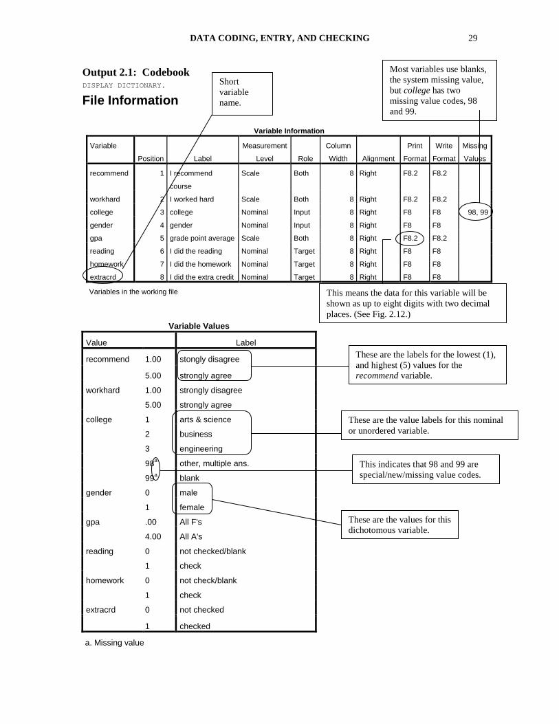
Select File → Display Data File Information → Working File. Your codebook should
look like Output 2.1, without the callout boxes. The codebook is divided into parts: the
Variable Information (which is very similar to the variable view in Fig. 2.12) and the
Variable Values (which are partially hidden in the variable view).
You may not be able to see all of the file information/codebook on your computer screen.
However, you should be able to print the entire codebook.
Fig. 2.12. Completed variable view.
DATA CODING, ENTRY, AND CHECKING 29
Output 2.1: Codebook
DISPLAY DICTIONARY.
File Information
Variable Information
Variable
Position Label
Measurement
Level Role
Column
Width Alignment
Format
Write
Format
Missing
Values
recommend 1 I recommend
course
Scale Both 8 Right F8.2 F8.2
workhard 2 I worked hard Scale Both 8 Right F8.2 F8.2
college 3 college Nominal Input 8 Right F8 F8 98, 99
gender 4 gender Nominal Input 8 Right F8 F8
gpa 5 grade point average Scale Both 8 Right F8.2 F8.2
reading 6 I did the reading Nominal Target 8 Right F8 F8
homework 7 I did the homework Nominal Target 8 Right F8 F8
extracrd 8 I did the extra credit Nominal Target 8 Right F8 F8
Variables in the working file
Variable Values
Value Label
recommend 1.00 stongly disagree
5.00 strongly agree
workhard 1.00 strongly disagree
5.00 strongly agree
college 1 arts & science
2 business
3 engineering
98a other, multiple ans.
99a blank
gender 0 male
1 female
gpa .00 All F's
4.00 All A's
reading 0 not checked/blank
1 check
homework 0 not check/blank
1 check
extracrd 0 not checked
1 checked
a. Missing value
This means the data for this variable will be
shown as up to eight digits with two decimal
places. (See Fig. 2.12.)
Most variables use blanks,
the system missing value,
but college has two
missing value codes, 98
and 99.
Short
variable
name.
These are the labels for the lowest (1),
and highest (5) values for the
recommend variable.
These are the value labels for this nominal
or unordered variable.
This indicates that 98 and 99 are
special/new/missing value codes.
These are the values for this
dichotomous variable.
30 CHAPTER 2
Problem 2.4: Enter Data
Close the codebook, and then click on the Data View tab on the bottom of the screen to give you
the data editor. Note that the spreadsheet has numbers down the left-hand side (see Fig. 2.13).
These numbers represent each subject in the study. UThe data for each participant’s questionnaire
go on one and only one line across the pageU with each column representing a variable from our
questionnaire. Therefore, the first column will be recommend, the second will be workhard, the
third will be college, and so forth.
After defining and labeling the variables, your next task is to enter the data directly from the
questionnaires or from a data entry form.
Sometimes researchers transfer the data from the questionnaires to a data entry form (like Table
2.1) by hand before entering the data into SPSS. This may be helpful if the questionnaires or
answer sheet are not easily readable by the data entry person, if the responses are to be entered
from several different sources, or if additional coding or recoding is required before data entry. In
these situations, you could make mistakes entering the data directly from the questionnaires. On
the other hand, if you use a data entry form, you could make copying mistakes, and it takes time
to transfer the data from questionnaires to the data entry form. Thus, there are advantages and
disadvantages of using a data entry form as an intermediate step between the questionnaire and
the data editor. Our cleaned up questionnaires should be easy enough to use so that you could
enter the data directly from Fig. 2.1 and Fig. 2.4 into the data editor. Try to do that using the
directions below. If you have difficulty, you may use Table 2.1, but remember that it took an
extra step to produce.
In Table 2.1, the data are shown as they would look if we copied the cleaned up data from the
questionnaires to a data entry sheet, except that the data entry form could be handwritten on ruled
paper.
Recommend Workhard College Gender Gpa Reading Homework Extracrd
1 3 5 1 0 3.12 0 0 1
2 4 5 2 0 2.91 1 1 0
3 4 5 1 1 3.33 0 1 1
4 5 5 1 1 3.60 1 1 1
5 4 5 2 1 2.52 0 0 1
6 5 5 3 1 2.98 1 0 0
7 4 5 2 0 2.50 1 0 0
8 2 5 98 0 2.20 0 0 0
9 5 5 3 0 3.00 0 1 0
10 99
11 3.5 5 1 1 9.67 1 1 0
12 2.5 5 2 1 1 1 1
To enter the data, ensure that your Data Editor is showing.
If it is not already highlighted, click on the far left column, which should say recommend.
To enter the data into this highlighted column, simply Utype Uthe number and press the right
arrow. For example, first type 3 (the number will show up in the blank space above the row
Table 2.1. A Data Entry Form: Responses Copied From the Questionnaires
DATA CODING, ENTRY, AND CHECKING 31
of variable names) and then press the right arrow; the number will be entered into the
highlighted box. Next, type 5 in the workhard column and so forth.
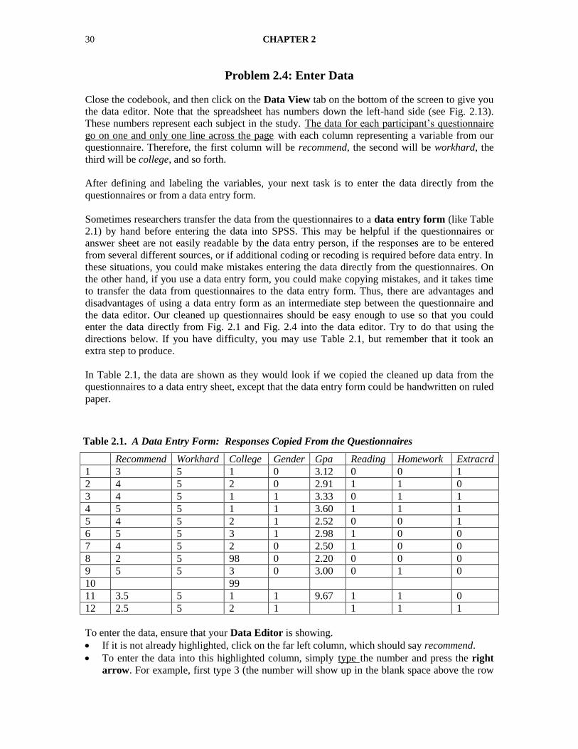
In Fig. 2.13, all the data for the participants have been entered.
Fig. 2.13. Data Editor participants entered.
Now enter from your cleaned up questionnaires the data in Fig. 2.1 and Fig. 2.4. If you make
a mistake when entering data, correct it by clicking on the cell (the cell will be highlighted),
type the correct score, and press enter or the arrow key.
Before you do any analysis, Ucompare the data on your questionnaires with the data in the Data
Editor.U If you have lots of data, a sample can be checked, but it is preferable to check all of the
data. If you find errors in your sample, you should check all the entries.
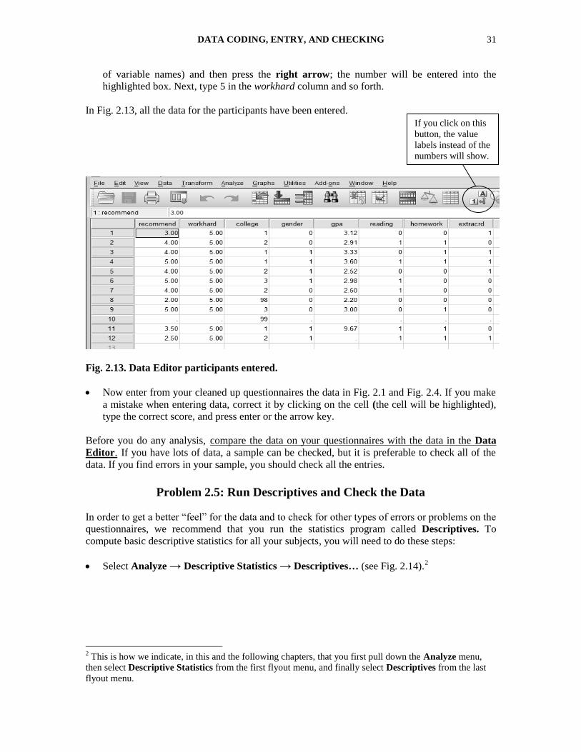
Problem 2.5: Run Descriptives and Check the Data
In order to get a better ―feel‖ for the data and to check for other types of errors or problems on the
questionnaires, we recommend that you run the statistics program called Descriptives. To
compute basic descriptive statistics for all your subjects, you will need to do these steps:
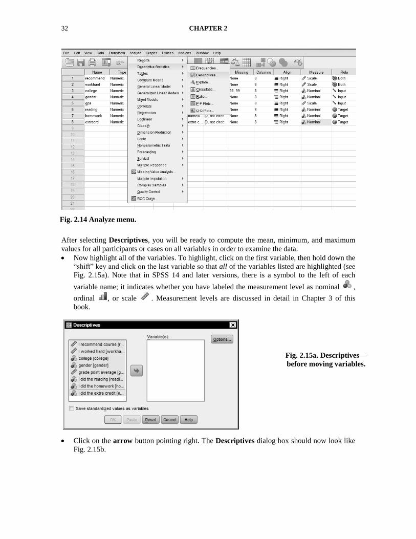
Select Analyze → Descriptive Statistics → Descriptives… (see Fig. 2.14).F
2
2 This is how we indicate, in this and the following chapters, that you first pull down the Analyze menu,
then select Descriptive Statistics from the first flyout menu, and finally select Descriptives from the last
flyout menu.
If you click on this
button, the value
labels instead of the
numbers will show.
in each cell.
32 CHAPTER 2
After selecting Descriptives, you will be ready to compute the mean, minimum, and maximum
values for all participants or cases on all variables in order to examine the data.
Now highlight all of the variables. To highlight, click on the first variable, then hold down the
―shift‖ key and click on the last variable so that all of the variables listed are highlighted (see
Fig. 2.15a). Note that in SPSS 14 and later versions, there is a symbol to the left of each
variable name; it indicates whether you have labeled the measurement level as nominal ,
ordinal , or scale . Measurement levels are discussed in detail in Chapter 3 of this
book.
Click on the arrow button pointing right. The Descriptives dialog box should now look like
Fig. 2.15b.
Fig. 2.15a. Descriptives—
before moving variables.
Fig. 2.14 Analyze menu.
DATA CODING, ENTRY, AND CHECKING 33
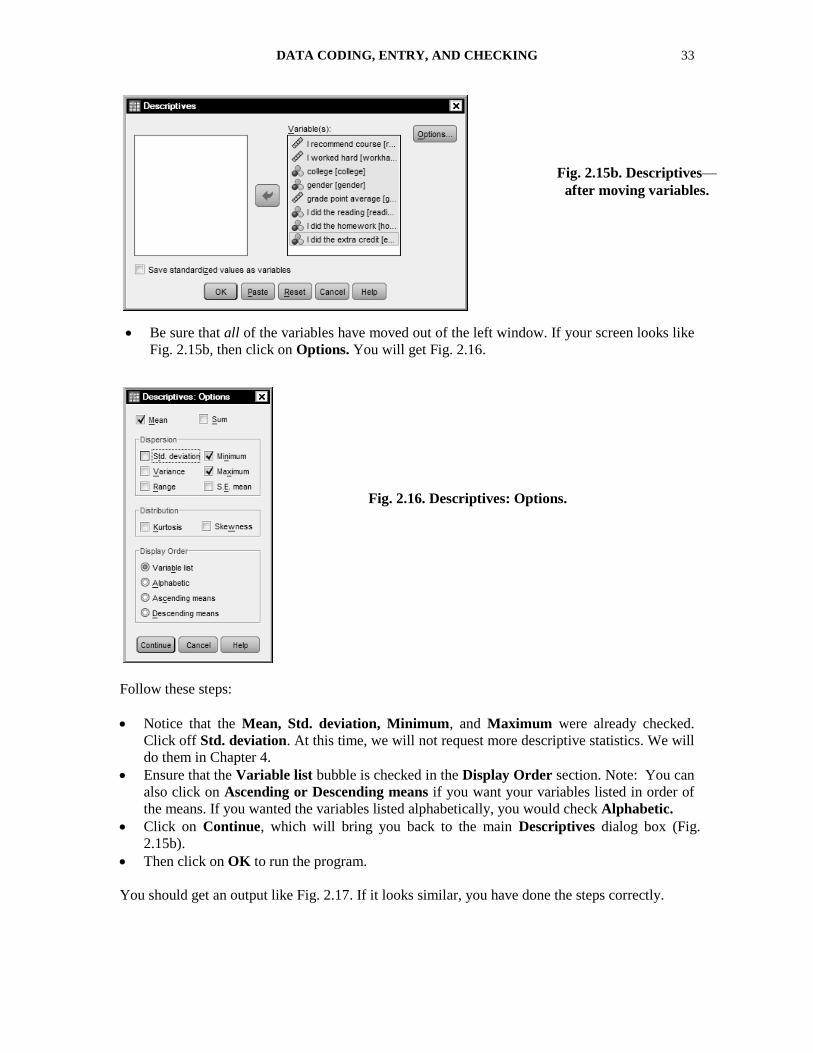
Be sure that all of the variables have moved out of the left window. If your screen looks like
Fig. 2.15b, then click on Options. You will get Fig. 2.16.
Follow these steps:
Notice that the Mean, Std. deviation, Minimum, and Maximum were already checked.
Click off Std. deviation. At this time, we will not request more descriptive statistics. We will
do them in Chapter 4.
Ensure that the Variable list bubble is checked in the Display Order section. Note: You can
also click on Ascending or Descending means if you want your variables listed in order of
the means. If you wanted the variables listed alphabetically, you would check Alphabetic.
Click on Continue, which will bring you back to the main Descriptives dialog box (Fig.
2.15b).
Then click on OK to run the program.
You should get an output like Fig. 2.17. If it looks similar, you have done the steps correctly.
Fig. 2.15b. Descriptives—
after moving variables.
Fig. 2.16. Descriptives: Options.
34 CHAPTER 2
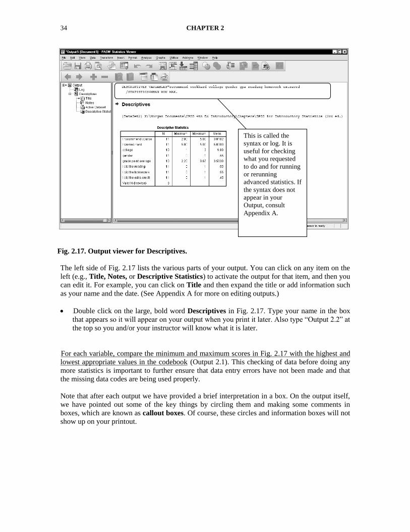
Fig. 2.17. Output viewer for Descriptives.
The left side of Fig. 2.17 lists the various parts of your output. You can click on any item on the
left (e.g., Title, Notes, or Descriptive Statistics) to activate the output for that item, and then you
can edit it. For example, you can click on Title and then expand the title or add information such
as your name and the date. (See Appendix A for more on editing outputs.)
5BDouble click on the large, bold word Descriptives in Fig. 2.17. Type your name in the box
that appears so it will appear on your output when you print it later. Also type ―Output 2.2‖ at
the top so you and/or your instructor will know what it is later.
UFor each variable, compare the minimum and maximum scores in Fig. 2.17 with the highest and
lowest appropriate values in the codebookU (Output 2.1). This checking of data before doing any
more statistics is important to further ensure that data entry errors have not been made and that
the missing data codes are being used properly.
Note that after each output we have provided a brief interpretation in a box. On the output itself,
we have pointed out some of the key things by circling them and making some comments in
boxes, which are known as callout boxes. Of course, these circles and information boxes will not
show up on your printout.
This is called the
syntax or log. It is
useful for checking
what you requested
to do and for running
or rerunning
advanced statistics. If
the syntax does not
appear in your
Output, consult
Appendix A.
DATA CODING, ENTRY, AND CHECKING 35
Output 2.2: Descriptives DESCRIPTIVES VARIABLES=recommend workhard college gender gpa reading homework extracrd
/STATISTICS=MEAN STDDEV MIN MAX .
Descriptives
Descriptive Statistics
11 2.00 5.00 3.8182
11 5.00 5.00 5.0000
10 1 3 1.80
11 0 1 .55
10 2.20 9.67 3.5830
11 0 1 .55
11 0 1 .55
11 0 1 .45
9
I recommend course
I worked hard
college
gender
grade point average
I did the reading
I did the homework
I did the extra credit
Valid N (l istwise)
N Minimum Maximum Mean
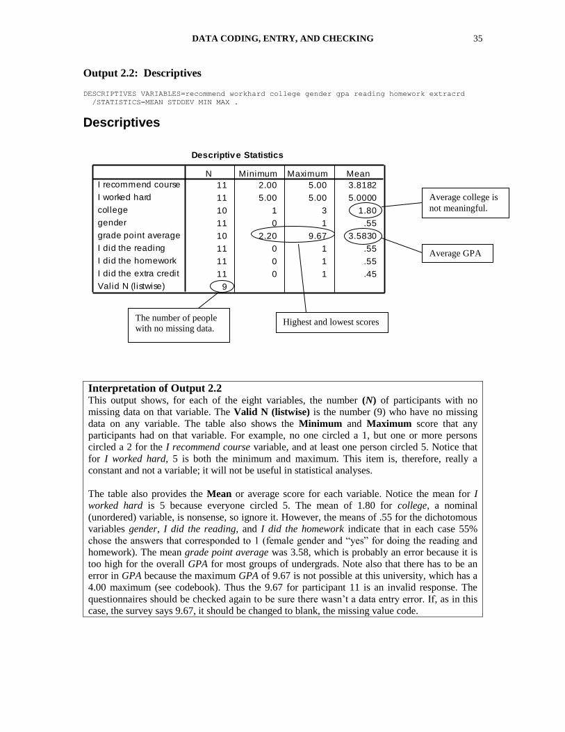
Interpretation of Output 2.2
This output shows, for each of the eight variables, the number (N) of participants with no
missing data on that variable. The Valid N (listwise) is the number (9) who have no missing
data on any variable. The table also shows the Minimum and Maximum score that any
participants had on that variable. For example, no one circled a 1, but one or more persons
circled a 2 for the I recommend course variable, and at least one person circled 5. Notice that
for I worked hard, 5 is both the minimum and maximum. This item is, therefore, really a
constant and not a variable; it will not be useful in statistical analyses.
The table also provides the Mean or average score for each variable. Notice the mean for I
worked hard is 5 because everyone circled 5. The mean of 1.80 for college, a nominal
(unordered) variable, is nonsense, so ignore it. However, the means of .55 for the dichotomous
variables gender, I did the reading, and I did the homework indicate that in each case 55%
chose the answers that corresponded to 1 (female gender and ―yes‖ for doing the reading and
homework). The mean grade point average was 3.58, which is probably an error because it is
too high for the overall GPA for most groups of undergrads. Note also that there has to be an
error in GPA because the maximum GPA of 9.67 is not possible at this university, which has a
4.00 maximum (see codebook). Thus the 9.67 for participant 11 is an invalid response. The
questionnaires should be checked again to be sure there wasn’t a data entry error. If, as in this
case, the survey says 9.67, it should be changed to blank, the missing value code.
Highest and lowest scores
Average GPA
Average college is
not meaningful.
The number of people
with no missing data.
36 CHAPTER 2
0BInterpretation Questions
2.1. What steps or actions should be taken after you collect data and before you run the analyses
aimed at answering your research questions or testing your research hypotheses?
2.2. Are there any other rules about data coding of questionnaires that you think should be
added? Are there any of our ―rules‖ that you think should be modified? Which ones? How
and why?
2.3. Why would you print a codebook or dictionary?
2.4. If you identified other problems with the completed questionnaires, what were they? How
did you decide to handle the problems and why?
2.5. If the university in the example allowed for double majors in different colleges (such that it
would actually be possible for a student to be in two colleges), how would you handle cases
in which 2 colleges are checked? Why?
2.6 (a) Why is it important to check your raw (questionnaire) data before and after entering
them into the data editor? (b) What are ways to check the data before entering them? After
entering them?
1BExtra Problems
Using the college student data.sav file, from www.psypress.com/ibm-spss-intro-statistics or the
Moodle Web site for this book, do the following problems. Print your outputs and circle the key
parts for discussion.
2.1 Compute the N, minimum, maximum, and mean for all the variables in the college student
data file. How many students have complete data? Identify any statistics on the output that
are not meaningful. Explain.
2.2 What is the mean height of the students? What about the average height of the same sex
parent? What percentage of students are males? What percentage have children?
Related Documents