Tax Deductions, Consumption Distortions,

Tax Deductions, Consumption Distortions,and the Marginal Excess Burden of Taxation

Ian W. H. Parry

Discussion Paper 99-48

August 1999

1616 P Street, NWWashington, DC 20036Telephone 202-328-5000Fax 202-939-3460Internet: http://www.rff.org

© 1999 Resources for the Future. All rights reserved.No portion of this paper may be reproduced withoutpermission of the author.

Discussion papers are research materials circulated by theirauthors for purposes of information and discussion. Theyhave not undergone formal peer review or the editorialtreatment accorded RFF books and other publications.

ii

Tax Deductions, Consumption Distortions,and the Marginal Excess Burden of Taxation

Ian W. H. Parry

Abstract

Certain types of expenditure--e.g. mortgage interest and medical insurance--receivefavorable tax treatment and are effectively subsidized relative to other (non-tax-favored)expenditures. Labor taxes (e.g. income taxes) can therefore produce efficiency losses bydistorting the allocation of consumption, in addition to distorting the labor market. Usingevidence on the responsiveness of taxable income to changes in tax rates, a seminal study byFeldstein (1999) estimates that the marginal excess burden of taxation (MEB) could exceedunity, when the effects of tax deductions are taken into account. This is several times largerthan in previous studies of the MEB that focus exclusively on labor market effects.

This paper develops a "disaggregated" approach to estimating the MEB thatdecomposes welfare impacts in the market for labor and tax-favored consumption goods, anduses micro evidence on labor supply elasticities, the demand elasticity for mortgage interest,medical insurance, and so on. Based on Monte Carlo simulations, we find a 68 percentprobability that the MEB lies between .31 and .48 for government transfer spending andbetween .21 and .35 for public goods. These estimates are below Feldstein's, but are stillconsiderably higher (70 percent or more) than when we ignore tax deductions.

Key Words: welfare costs, tax system, tax deductions, simulations

JEL Classification Numbers: H21, H43

iii

Table of Contents

1. Introduction ................................................................................................................. 1

2. Deriving Formulas for the MEB in the Presence of Tax Deductible Spending .............. 5

A. Model Assumptions ............................................................................................. 5

B. The MEB for Transfer Spending .......................................................................... 8

C. The MEB for Public Goods ................................................................................. 9

3. Estimating the MEB ...................................................................................................11

A. Parameter Values ................................................................................................11

Labor supply elasticities .....................................................................................11

Labor tax rate .....................................................................................................11

Components of the tax-favored sector .................................................................13

Demand elasticities for tax-favored goods ..........................................................15

Tax-subsidy rates ................................................................................................15

B. Results ................................................................................................................16

C. Monte Carlo Analysis .........................................................................................18

4. Further Discussion: Non-Tax Distortions in Markets with Tax-Subsidies ....................19

Housing ......................................................................................................................19

Medical Services ........................................................................................................21

Charitable Contributions .............................................................................................22

5. Conclusion .................................................................................................................22

Appendix ............................................................................................................................24

References ..........................................................................................................................26

List of Tables and Figures

Table 1. Estimated Losses in Personal Income Tax Revenues by Function (1995) ............14

Table 2. Calculations of the MEB ....................................................................................17

Figure 1. Probability Distributions for the MEB ................................................................20

1

TAX DEDUCTIONS, CONSUMPTION DISTORTIONS,AND THE MARGINAL EXCESS BURDEN OF TAXATION

Ian W. H. Parry*

1. INTRODUCTION

Public expenditure programs on defense, education, medical care, assistance for thepoor, pensions, crime prevention, and so on, obviously produce potentially important benefitsfor society. But these programs also entail social costs and--at least on the criterion ofeconomic efficiency--additional spending on any of these programs is worthwhile only if thesocial benefits that are generated exceed the extra social costs. Economists have longrecognized that the social costs of public spending include not only the opportunity costs ofthe resources involved, but also the resulting deadweight loss from higher distortionary taxesthat are necessary to finance the spending (Pigou, 1947; Harberger, 1964; Browning, 1976).1

This paper is about the estimation of these deadweight losses for the US economy.Over the years a number of studies have attempted to estimate the marginal excess

burden of taxation (MEB).2 This is the efficiency loss from the increase in distortionary taxesnecessary to raise an extra dollar of tax revenue. Traditionally, studies have focussed on theefficiency impact of the tax increase in factor markets alone, particularly the labor market.Estimates of the MEB vary a lot due, among other things, to different assumptions aboutrelevant elasticities, which tax is being increased, and what the extra spending is used for.But a central estimate from this literature for the MEB of labor taxation, when the dollar isreturned to households in a transfer payment, is about 25 cents.3

However, some very recent studies have emphasized that the tax system distorts notonly factor markets, but also the allocation of spending among different types of consumption,saving, and investment. This is because certain types of expenditures, such as mortgage

* Fellow, Energy and Natural Resources Division, Resources for the Future. The author is grateful to AntonioBento and Rob Williams for very helpful comments and suggestions. Don Crocker provided first-rate researchassistance. Correspondence to: Ian Parry, Resources for the Future, 1616 P Street, Washington, D.C. 20036.Phone: (202) 328-5151, email: [email protected] More generally, extra spending can be financed by cutting back other spending programs, or by increasingborrowing. In the latter case, tax increases are effectively delayed until a future period. We focus purely on thecase when spending is financed from current taxes.2 This is sometimes referred to as the marginal welfare cost of taxation. A related concept is the marginal costof public funds which we discuss below.3 Notable contributions that employ static models include Ballard (1990), Browning (1976, 1987, 1994),Mayshar (1991), Stuart (1984), and Wildasin (1984). Ballard et al. (1985) presents results from a dynamiccomputable general equilibrium model that allows for tax increases on both labor and capital (see footnote 31below). Snow and Warren (1996) and Fullerton (1991) attempt to reconcile the variation in estimates acrossdifferent studies.

Ian W. H. Parry RFF 99-48

2

interest, employer-provided medical insurance and other fringe benefits, pension andcharitable contributions, interest on local government bonds, and so on, receive favorable taxtreatment, and therefore are effectively subsidized relative to other types of spending.Increasing the rates of existing taxes may therefore produce efficiency losses not only byincreasing tax distortions in factor markets, but also by increasing subsidy distortions for tax-favored expenditures.

The recent studies have attempted to estimate the tax income elasticity (TIE). Thiselasticity captures the effect of changes in marginal income tax rates on reducing peoples'reported taxable income, both through reducing labor supply and by substituting tax-favoredspending for non tax-favored expenditure. Initially, estimates for the TIE using 1980's datawere quite high--typically greater than one (e.g. Feldstein, 1995; Lindsey, 1987). Animportant paper by Feldstein (1999) demonstrates that such high elasticities would implydramatically larger values for the MEB, well above one dollar for transfer spending. This is avery striking result: it would imply that the social benefits of (marginal) public spending mayhave to exceed two dollars per dollar of extra spending in order to be justified on the groundsof economic efficiency! More recent studies using 1990's data, however, point towardssomewhat smaller values for the TIE (see e.g. Auten and Carroll, 1998; Carroll, 1998a),implying the MEB might be closer to 0.5 than unity.4

There are important advantages to using estimates of the TIE to infer the MEB. Inparticular, this approach minimizes information requirements because it involves theestimation of a single elasticity that summarizes a whole host of substitution possibilities foravoiding taxes. On the other hand, there are a number of respects in which the TIE literatureis preliminary at this stage.

First, the studies typically estimate the TIE by comparing the changes in taxableincome across taxpayer groups whose marginal tax rates were changed by different amountsfollowing tax legislation. This "differences in differences" approach is designed to control fornon-tax factors (e.g. business cycle effects) that have a proportional effect on the taxableincome of all groups during the period before and after the tax legislation. However, thismethod does not control for factors that affect income inequality. In periods of increasingincome inequality, such as the 1980s and 1990s, when marginal tax rates for higher incomegroups fall (rise) relative to those for other groups, comparing the change in taxable income ofthese groups can produce estimates of the TIE that are biased upwards (downwards). Sincethe 1986 Tax Reform Act reduced marginal tax rates, while the 1990 and 1993 BudgetAgreements increased them, studies using 1980's data may overstate the TIE, while studiesusing 1990's data may understate it.

4 This is based on my own rough calculations, using estimates of the TIE in Carroll (1998b), Table 1. Inaddition to its use in project evaluation, the MEB is also a crucial determinant of the welfare effects of tax shifts(i.e. simultaneous changes in different tax rates that keep the overall level of tax revenue the same). For adiscussion of how tax deductions, through their effect on the MEB, crucially influence the efficiency impact ofswapping environmental taxes for other taxes see Parry and Bento (1999).


3

Second, what matters for the MEB is the long run equilibrium responses to changes intax rates. The short run responses that are often the focus of the econometric studies may bemore pronounced than the long run changes due to transitory shifts in taxable income. Forexample, people may temporarily postpone selling stocks in anticipation of lower capitalgains taxation, thereby exaggerating the increase in taxable income before and after a taxreduction. In other respects the short run response may understate the long run response. Forexample, the full effects of changes in the effective tax-subsidy for mortgage interest on thestock of owner occupied housing may occur with a considerable lag.

Third, in practice the price distortions in the markets for tax-favored consumptiongoods often depend on a number of other factors besides the subsidy from federal taxprovisions. For example, future income from pension accumulations is subject to taxationthat offsets the subsidy for current, tax-deductible contributions, at least to some extent. Morespending on charities may increase rather than reduce welfare if there are significantbeneficial externalities. Economic efficiency in the housing market is affected by propertytaxes, housing assistance programs, external benefits and costs, and so on. These other typesof pre-existing "distortions" are not taken into account when (unadjusted) estimates of the TIEare used to calculate the MEB.

In addition the studies focus on the behavior of subgroups of taxpayers rather than thebehavior of all actual and potential taxpayers. These subgroups usually consist of higherincome taxpayers that generally itemize deductions and therefore may be more responsive totax changes than the average taxpayer. Some studies are based on the tax returns of marriedcouples which may display a relatively high sensitivity to tax changes--for example, most ofthe responsiveness of labor supply comes from the participation decision of married (female)workers rather than the overtime behavior of non-married workers. Finally, to date studieshave estimated only the compensated TIE. However, estimating the MEB for different typesof public expenditure, and particularly public goods, can also require estimates ofuncompensated price effects (see below).5

Many of these limitations should be overcome, at least to some extent, as econometricstudies of the TIE are refined over time. However, particularly while there is still significantuncertainty over the TIE, it seems worthwhile to make use of other evidence that can behelpful in gauging the magnitude of the MEB. In this paper we present a "disaggregated"approach to estimating the MEB in the presence of tax deductions. This involves adding upthe welfare impacts of tax increases in the labor market and the markets for individual tax-favored goods. One virtue of this approach is that it makes transparent the potentialcontribution of underlying parameters to the MEB--e.g. the demand elasticity for medicalinsurance, the magnitude of the assumed pre-existing distortion in the housing sector--whichare not revealed in the TIE studies. Unfortunately, there is uncertainty about the values ofthese underlying parameters, and therefore we would not necessarily claim that our approach

5 For a more comprehensive discussion of the methodological issues involved in estimating the TIE see Triest(1998), Slemrod (1998), and Carroll (1998b).


4

yields more accurate calculations of the MEB than those based on estimates of the TIE.Nonetheless, it is still helpful to explore the consistency between estimates of the MEB basedon the TIE, with estimates based on micro evidence about underlying parameters.

We begin in the next section by deriving formulas for the MEB in the presence of taxdeductions, under alternative assumptions concerning the disposition of government revenues.Our analysis is static--as in Feldstein (1999)--and captures the impact of the tax system ondistorting the labor/leisure decision and the choice among consumption goods. This providesconservative estimates of the MEB (though how conservative is unclear), since we do notcapture the impact of the tax system on distorting the consumption/savings decision and thechoice among different types of investment. Thus, we do not model tax deductions forpension contributions, accelerated depreciation, and so on.

Section 3 presents calculations of the MEB based on what we believe are plausibleparameter values. In the absence of tax deductions (i.e. focussing on efficiency impacts in thelabor market alone) the MEB for government transfer payments ranges from 0.1 to 0.42, witha central value of 0.22.6 Incorporating tax deductions, the range becomes 0.15 to 0.92, with acentral value of 0.39. For individual deductions to make much difference to the MEB the taxexpenditure involved must be significant relative to aggregate labor tax revenues, and theymust be applied to spending that exhibits a fair amount of price sensitivity. The huge bulk ofthe increase in the MEB is due to welfare impacts in the housing and medical insurancemarkets alone.

Clearly, this is a wide range of possible outcomes for the MEB. We perform MonteCarlo experiments to try and narrow the range and perhaps make the results more useful forproject evaluation. According to these results, we find a 68 percent probability that the MEBfor transfer spending lies between 0.31 and 0.48. These results clearly underscore Feldstein'soriginal insights about the importance of tax deductions--for example our central estimate is77 percent higher when we include tax deductions. However, our estimates are lower than inFeldstein (1999), partly because we exclude certain deductions from our analysis that do notdirectly distort the consumption bundle.

For public goods (that are separable in the utility function) our central estimate for theMEB increases from 0.13 to 0.27 when we allow for tax deductions. Our Monte Carlosimulations suggest a 68 percent probability that the MEB for public goods lies between 0.21and 0.35. These numbers are lower than for transfer spending, due to the familiar incomeeffects than dampen the change in labor supply (see below). However, they are well above 0unlike in some other studies that do not take account of tax deductions (see Ballard andFullerton, 1992, for a good discussion).

In section 4 we briefly discuss the literature on distortions in tax-favored sectors(externalities, other regulations, etc.). These sources of non-tax distortion are sometimesoffsetting and are generally difficult to quantify. Although we exclude most of these factors,

6 Loosely speaking, transfer payments may represent such things as social security benefits, and public spendingthat is a close substitute for private spending (e.g. medical services, education, food stamps).


5

it is straightforward to infer from our formulas how alternative assumptions about the size ofthese distortions, relative to the tax-subsidy, would affect our calculations of the MEB.

Section 5 concludes and discusses some limitations of our analysis. In particular, ouranalysis does not capture the discounted welfare effects from changes in the future path ofinvestments in tax-favored and non-tax-favored assets.

2. DERIVING FORMULAS FOR THE MEB IN THE PRESENCE OF TAXDEDUCTIBLE SPENDING

In this section we describe the assumptions underlying our analytical model and deriveformulas for the MEB for the case of government transfer payments and public goods.

A. Model Assumptions

We assume a static economy where the representative household has the followingutility function:7

( ) )(,,,...,1P

M GLLyxxuU φ+−= (2.1)

where u(.) is continuous and quasi-concave and φ′ > 0. The xi's denote consumer goods thatreceive favorable tax treatment one way or another. These include untaxed, in-kindcompensation for labor supply, or fringe benefits, and the most important example in thiscategory is employer-provided medical insurance. The xi's also include goods that can bededucted from taxable income. The most important example in this category is mortgageinterest on owner occupied housing, which roughly reflects housing services for homeowners.y denotes an aggregate of all other "ordinary" consumption (i.e. that does not receivefavorable tax treatment). LL − is leisure time, and this equals the household timeendowment ( L ) less labor supply (L). GP is the quantity of a public good provided by thegovernment.8

Competitive firms produce the consumption goods using labor as the only input.More generally of course, capital is an important input--although the labor market is aboutthree times as large as the capital market. Incorporating capital goods would require adynamic analysis in which the tax system distorts the labor/leisure decision, the

7 Our assumption of homogeneous agents implies that we abstract from distributional considerations. Moregenerally, progressive increases in the rates personal income tax could produce non-economic gains for societythat effectively reduce the MEB by creating a more equitable net-of-tax income distribution (see e.g. Mirrlees,1994, p. 226, for more discussion).8 For our purposes we simplify by assuming public goods are separable in the utility function (or put anotherway, private consumption and public goods are "ordinary independents" (Wildasin, 1984). More generally ifpublic goods are a complement (substitute) for leisure, then additional public spending will lead to a feedbackeffect that reduces (increases) labor supply (see Atkinson and Stern, 1974). As a result, the MEB for publicgoods will be higher (lower). In practice however, estimating these types of feedback effects is difficult.Moreover, in some important cases (e.g. national defense) it seems reasonable to assume that more of the publicgood would not affect the marginal value of labor time relative to leisure time for the representative household.


6

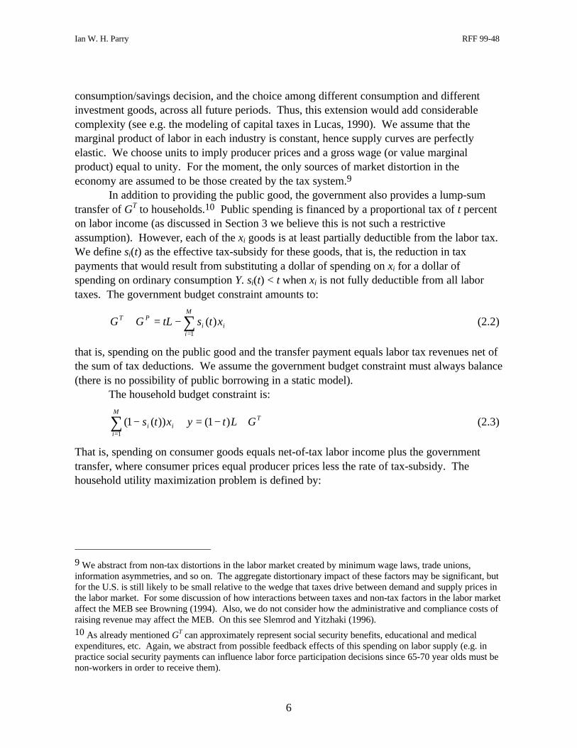
consumption/savings decision, and the choice among different consumption and differentinvestment goods, across all future periods. Thus, this extension would add considerablecomplexity (see e.g. the modeling of capital taxes in Lucas, 1990). We assume that themarginal product of labor in each industry is constant, hence supply curves are perfectlyelastic. We choose units to imply producer prices and a gross wage (or value marginalproduct) equal to unity. For the moment, the only sources of market distortion in theeconomy are assumed to be those created by the tax system.9

In addition to providing the public good, the government also provides a lump-sumtransfer of GT to households.10 Public spending is financed by a proportional tax of t percenton labor income (as discussed in Section 3 we believe this is not such a restrictiveassumption). However, each of the xi goods is at least partially deductible from the labor tax.We define si(t) as the effective tax-subsidy for these goods, that is, the reduction in taxpayments that would result from substituting a dollar of spending on xi for a dollar ofspending on ordinary consumption Y. si(t) < t when xi is not fully deductible from all labortaxes. The government budget constraint amounts to:

∑=

−=+M

iii

PT xtstLGG1

)( (2.2)

that is, spending on the public good and the transfer payment equals labor tax revenues net ofthe sum of tax deductions. We assume the government budget constraint must always balance(there is no possibility of public borrowing in a static model).

The household budget constraint is:

TM

iii GLtyxts +−=+−∑

=

)1())(1(1

(2.3)

That is, spending on consumer goods equals net-of-tax labor income plus the governmenttransfer, where consumer prices equal producer prices less the rate of tax-subsidy. Thehousehold utility maximization problem is defined by:

9 We abstract from non-tax distortions in the labor market created by minimum wage laws, trade unions,information asymmetries, and so on. The aggregate distortionary impact of these factors may be significant, butfor the U.S. is still likely to be small relative to the wedge that taxes drive between demand and supply prices inthe labor market. For some discussion of how interactions between taxes and non-tax factors in the labor marketaffect the MEB see Browning (1994). Also, we do not consider how the administrative and compliance costs ofraising revenue may affect the MEB. On this see Slemrod and Yitzhaki (1996).10 As already mentioned GT can approximately represent social security benefits, educational and medicalexpenditures, etc. Again, we abstract from possible feedback effects of this spending on labor supply (e.g. inpractice social security payments can influence labor force participation decisions since 65-70 year olds must benon-workers in order to receive them).


7

( ) )(,,...,,),,( 21P

MPT GLLyxxxuMAXGGtV φ+−= (2.4)

−−−−++ ∑=

yxtsLtGM

iii

T

1

))(1()1(λ

where V(.) is the indirect utility function and the Lagrange multiplier λ is the marginal utilityof income. The solution to this problem yields the uncompensated demand and labor supplyfunctions:

),( Tii Gtxx = ; ),( TGtyy = ; ),( TGtLL = (2.5)

(these functions are independent of GP, given the separability in (2.1)). From differentiatingthe indirect utility function (2.4) we obtain.

′−−=

∂∂ ∑

=

M

iii xsL

tV

1

λ ; λ=∂∂

TGV

; φ ′=∂∂

PGV

(2.6)

We now define the MEB for spending on the lump sum transfer (MEBT) and on thepublic good (MEBP). These cases correspond to when public spending is a perfect substitutefor private consumption, and when it has zero substitutability with private consumption,respectively. More generally of course, public spending may be a partial substitute for privatespending. We do not explicitly consider this case, since it can easily be inferred by taking theappropriate weighted-average of MEBT and MEBP.11

We define the MEB by the welfare loss arising from equilibrium quantity changes inmarkets distorted by the tax system, following an extra dollar of tax-financed spending. Thisis the welfare loss that should be subtracted from a partial equilibrium benefit/cost calculationof incremental public spending and corresponds to the definition that is often used in theliterature (e.g. Stuart, 1984; Ballard and Fullerton, 1992; Ballard et al., 1985). Weacknowledge that other definitions are possible, and perhaps preferable, and (as noted inSection 3) would imply somewhat different empirical results.12

11 Kormendi (1983) and Aschauer (1985) find that one dollar of general government spending (i.e. transfers pluspublic goods) reduces private spending by about 30 cents. In this case, using the results below, we wouldcalculate the MEB as 0.3 MEBT + 0.7 MEBP. It is important to understand, however, that our analysis is notapplicable to redistributive government programs. For these policies we would need to disaggregate thehousehold sector into different income groups and explore how the policy affects the behavior of each group.The MEB tends to be much higher for redistributive programs relative to other government programs (seeBrowning, 1986).12 In Browning (1987) the MEB is the excess of social benefits over the dollar outlay that is necessary to keephouseholds at the same level of utility, following a dollar increase in public spending financed by increasing adistortionary tax. In this case the MEB depends only on compensated elasticities. In contrast, some of theelasticities in our formulas are uncompensated reflecting income effects. This issue is discussed further below.See Browning et al. (1997) for a discussion of alternative definitions of the MEB.


8

B. The MEB for Transfer Spending

We define the MEB for an extra dollar of spending on the lump-sum transfer (holdingGP fixed) as follows:

dtdG

dtdV

MEBT

T λ1

−= (2.7)

where

dtdG

G

VtV

dtdV T

T∂∂

+∂∂

= (2.8)

The numerator in (2.7) is the utility loss, expressed in dollars, from an incremental increase inthe labor tax. In (2.8) this is decomposed into the effect of the increase in tax and the increasein spending. The denominator in (2.7) is the (general equilibrium) increase in transferspending enabled by the increase in labor tax. Thus the MEB is the welfare loss fromincreasing the labor tax, per dollar of extra spending on GT.

From (2.6)-(2.8):

11 −′−

=∑

=

dtdG

xsLMEB

T

M

iii

T (2.9)

From totally differentiating the government budget constraint (2.2) using (2.5) we can obtain:

dtt

xsxs

tL

tLdGG

xs

G

Lt

M

i

ii

M

iii

TM

iTi

iT

∂∂

−′−∂∂

+=

∂∂

+∂∂

− ∑∑∑=== 111

1 (2.10)

From the Slutsky equations:

′−∂∂

−∂

∂=

∂∂ ∑

=

M

iiiT

c

xsLGL

tL

tL

1

;

′−∂∂

−∂

∂=

∂∂ ∑

=

M

iiiT

icii xsL

G

x

t

x

t

x

1

(2.11)

where "c" denotes a compensated coefficient and ii xsL ′∑− is the reduction in household

income from an uncompensated increase in the labor tax rate. Substituting (2.10) and (2.11)in (2.9) and dividing through by L gives:

∂∂

+′−∂∂

+

∂∂

+∂

∂−

=

∑ ∑

∑

= =

=

M

i

M

i i

iiiii

M

i

ci

i

ii

c

T

xt

xss

tL

Lt

t

x

x

s

tL

Lt

MEB

1 1

1

1π

π

π (2.12)


9

where πi = xi/L is the share of good xi in the total value of output. We define:

Lt

tLc

cL

−−∂

∂=

1

)1(ε ;

Lt

tLu

L

−−∂

∂=

1

)1(ε ;

i

i

i

cic

x x

s

s

xi

−−∂

∂−=

1

)1(η ;

i

i

i

iux x

s

s

xi

−−∂

∂−=

1

)1(η (2.13)

cLε and u

Lε are the compensated and uncompensated elasticity of labor supply with respect to the

household wage respectively, and cxi

η and uxi

η are the compensated and uncompensated elasticity

of demand for good xi (defined as positive numbers). Noting that )1(// tLtL −∂−∂=∂∂ ,

))1(/(/ iiii sxstx −∂∂′−=∂∂ , and so on, then from (2.12) and (2.13) we can obtain:

−

+′−−

−

′−

+−

=

∑

∑

=

=

M

i

ux

i

iii

uL

M

i

cxi

i

ii

cL

T

i

i

s

ss

tt

ss

s

tt

MEB

1

1

11

11

11

ηπε

ηπε (2.14)

There are several noteworthy points about this formula for the MEB.13 In the absenceof tax deductions (si = 0) the formula would be consistent with the MEB formulas derived inother studies for lump-sum transfers financed by proportional taxes (see e.g. Mayshar, 1991).The new terms in the numerator and denominator reflect the effect of higher taxes onincreasing subsidy distortions for tax-favored goods, and both serve to raise the MEB. Theseterms are larger: (a) the greater the size of these markets relative to the labor market (πi); (b)the greater the pre-existing wedge between the demand and supply price (si) (c) the greater theelasticity of demand for tax-favored goods (the u

xiη and c

xiη 's) and (d) the greater the impact of

higher taxes on increasing subsidy rates ( is′ ). Finally, the MEB formula in (2.14) depends on

both compensated and uncompensated elasticities. This is because the additional lump-sumincome partially--but not fully--compensates households for the reduction in household surplusfrom the tax increase (in other words dV/dt < 0).14

C. The MEB for Public Goods

Suppose instead that the extra dollar of spending was on the public good rather thanthe lump-sum transfer. In this case we define the MEB as:

13 Note that we have not placed certain restrictions on the utility function in deriving this formula, such as thecommonly used assumption in computable general equilibrium models that all consumption goods are equalsubstitutes for leisure. The formula would be more complicated if we allowed for differences in tax rates andelasticities across agents. In particular, if households facing higher than average tax rates also had higher (lower)than average labor supply and demand elasticities, then the MEB would be larger (smaller) than predicted by ourmodel. Browning (1987, footnote 8) suggests that allowing for dispersion in parameters across householdswould not greatly affect the estimated MEB.14 The denominator in (2.14) is positive for the range of parameter values used below. It could only be negativein the (unlikely) case that the labor tax Laffer curve is downward sloping.


10

)1/(

1

−′−−

= λφλ

dtdG

dtdV

MEBP

P (2.7′)

where

dtdG

tV

dtdV P

φ ′+∂∂

= (2.8′)

The expression in (2.7′) is the overall change in utility per dollar of additional spending on thepublic good, after netting out the direct benefit and resource cost of the extra spending.Again, this reflects the welfare impacts in markets distorted by the tax system.

Differentiating the government budget constraint holding GT constant gives:

dtt

xsx

dt

ds

tL

tLdGM

i

M

i

iii

iP

∂∂

−−∂∂

+= ∑ ∑= =1 1

(2.10′)

This expression is a little simpler than that in (2.10), since labor supply and the demand forgoods are not affected by the increase in public spending (i.e. there is no positive incomeeffect from the extra public spending to counteract the adverse income effect from the taxincrease). Following the same procedure as before, but using (2.7′), (2.8′) and (2.10′), insteadof (2.7), (2.8) and (2.10), we obtain:

−

+′−−

−

−′+

−=

∑

∑

=

=

M

i

ux

i

iii

uL

M

i

ux

i

iii

uL

P

i

i

s

ss

tt

s

ss

tt

MEB

1

1

11

11

11

ηπε

ηπε (2.14′)

The only difference between this formula and that in (2.14) is that all the elasticitiesare now uncompensated. This is because spending on the public good is not a substitute fordisposable income, and therefore does not compensate households for the income loss fromthe tax increase. This point has long been recognized in the literature. Indeed it has beenemphasized that the MEB for proportional labor taxes (without deductions) is negative if theuncompensated labor supply elasticity is negative (i.e. the labor supply curve is backwardbending).15 In practice this seems unlikely since the balance of empirical evidence suggeststhat the economy-wide uncompensated labor supply elasticity is positive (see below).Moreover, with tax deductions the MEB could still be positive even if the labor supplyelasticity is negative. This is because tax-favored consumption is a normal good, hence, evenif the first term in the numerator in (2.14′) is negative the second term is always positive.

15 See e.g. Wildasin (1984), Stewart (1984), Ballard and Fullerton (1992).


11

Finally, we note that 1 + MEBP is equivalent to the commonly used marginal cost ofpublic funds. This is simply the full cost of incremental spending on public goods, which isthe resource value of a dollar plus the incremental efficiency loss from higher taxes necessaryto raise an extra dollar of revenue.

3. ESTIMATING THE MEB

In this section we discuss plausible parameter values and what they imply for ourdefinitions of the MEB. We also present Monte Carlo simulations to indicate "most likely"outcomes from our range of possible values for the MEB.

A. Parameter Values

Labor supply elasticities

In our highly aggregated model, the labor supply response to changes in the net-of-taxwage reflects the impact on average hours per worker and the impact on the participation rateaveraged across all members (male and female) of the labor force. There is a sizeable literatureon labor supply elasticities for the United States (see e.g. the review in Killingsworth (1983))and we do not go into the details here. Based on a recent survey of labor economists' views byFuchs et al. (1998), we choose central values of 0.2 and 0.35 for the (economy-wide)uncompensated and compensated labor supply elasticities respectively, and plausible ranges forthese elasticities of 0.1-0.3 and 0.2-0.5.16 Note that there is a fair amount of uncertainty overthese important parameters.

Labor tax rate

The calculation of the labor tax rate is a little involved, and we provide more details inthe Appendix. We assume a central value of 36 percent for the labor tax, which we arrived atas follows. We estimate the average rate of labor tax, which is relevant for the labor forceparticipation decision, at 33 percent for 1995 (see Appendix). The contribution of varioustaxes is as follows: federal income taxes 12.7 percent, state income taxes 3.0 percent, payrolltaxes 10.8 percent, and sales and excise taxes 6.7 percent.17 The marginal rate of labor tax

16 These values are from Table 2 in Fuchs et al., assuming a weight of 0.6 and 0.4 for the male and femaleelasticities respectively. Taking labor supply elasticities averaged over all workers (rather than, for example,male workers only), more or less rules out the possibility of a negative uncompensated elasticity. The laborsupply estimates reported in Fuchs et al. may understate the overall change in effective labor supply to someextent since they do not take account of the potential for lower net-of-tax wages to discourage effort on the job,or induce long run changes in occupational choice. In comparing our estimates of the MEB to those fromcomputable general equilibrium models (e.g. Stuart, 1984; Ballard et al., 1985), it is noteworthy that the lattermodels often assume significantly higher values for the compensated labor supply elasticity (see the discussionin Browning, 1987, footnote 9).17 It is standard in the literature to assume in static models that sales and excise taxes are effectively borne bylabor.


12

affects the amount of hours per worker over a year (overtime, willingness to take a secondjob, etc.) and we assume a value of 41 percent for the typical worker (see Appendix). Sinceroughly two thirds of the estimated labor supply responses come from changes in participationrates and one third from changes in average hours (see e.g. Russek, 1996), we attachedweights of two thirds and one third for the average and marginal rate of tax, respectively, toobtain our value of 36 percent.18

This value is below labor tax rates assumed in most other studies of the MEB--forexample Ballard (1990) and Stewart (1984) used 40 percent and Browning (1987) assumed acentral value of 43 percent. The differences between these tax rates may seem small, but theyimply noticeably different values for the MEB. We prefer the lower value for two reasons.First, other studies use marginal tax rates, rather than a weighted average of marginal andaverage tax rates; thus they implicitly attribute all of the labor supply response to changes inhours per worker and none to the participation decision. Second, other studies often assumeall social security payments are effective taxes (though Feldstein, 1999, is a noticeableexception). In practice, workers do gain some offsetting benefits from these taxes in terms offuture social security benefits in retirement--although expected benefits are typically lowerthan they would be if workers could invest social security contributions in private capitalmarkets. Our figure includes an assumption that the effective burden of (non-Medicare)social security taxes is 30 percent lower than current tax payments due to future benefits,though there is much controversy surrounding this issue.19

Given the controversy about effective payroll taxes, variability in tax revenues overthe business cycle, and allowing for measurement errors, it is appropriate to consider a rangeof values for labor tax rates. We assume a range of 32 to 40 percent.

18 To incorporate a non-proportional labor tax in our model (i.e. to have separate rates for average and marginaltaxes) would require separating out the participation and hours worked decision. We think that the costs of thisextra complexity probably outweigh any benefits from slightly more accurate estimates of the MEB. Othermodels do not decompose these two dimensions of labor supply either, and implicitly assume that the marginalrate of tax is relevant for determining the participation as well as the hours worked decision. In this respect theyoverstate the MEB to some extent. Other models allow for the possibility that increases in the labor tax may be progressive (i.e. they increase themarginal rate of tax by more than the average rate), while our analysis is limited to proportional changes in taxes.This may not be a major drawback however, given that, as already explained, two thirds of the labor supplyresponse is governed by the increase in average rate of labor tax and only one third depends on the increase inmarginal rate of tax.19 This is because the link between future benefits and current payments is complicated by Social Security rules.For example, benefits are based on the 35 years of highest earnings, so that people under 30 may receive nobenefits for their current contributions. If 65-70 year olds decide to continue working they forgo benefitpayments. Benefits may be linked to a spouse's earnings, therefore someone may receive no benefits from theirown contributions. In addition, there is uncertainty over the amount of social security taxes that will be raisedfrom future workers to pay for the retirement benefits of current workers. See Feldstein and Samwick (1992) fora good discussion of these issues.


13

Components of the tax-favored sector

Table 1 shows estimates of federal revenue losses for various categories due todeductions and exemptions built into the income tax system for 1995, as reported in theStatistical Abstract of the United States. We divide these figures by 0.24--a typical estimateof the marginal rate of federal income tax faced by the average household (Feldstein, 1999)--in order to obtain dollar estimates of total spending on tax-favored goods. In turn, thesenumbers are divided by gross labor income ($3,849 billion--see Appendix) to obtain the πi'sreported in the last column.20

The two most important sectors that receive tax-subsidies are employer-providedmedical insurance and owner occupied housing services. These sectors amount to 5.6 and 5.0percent respectively of gross labor income. There are a variety of much smaller items thatadd another 1.5 percent (child-care, employee parking, and so on.).21

We exclude from our analysis a variety of other tax exemptions, shown in the lowerhalf of Table 1. These include deductions for savings and investment--pension contributions,interest on state and local bonds, capital gains at death, corporate income tax deductions, andinterest on life insurance savings. As already noted, a proper treatment of these deductionswould require a dynamic model with investment in different types of assets that are taxed orsubsidized at different rates, and is beyond the scope of this paper.22 Clearly these aresizeable deductions, however, which suggests that our static analysis is missing a significantpart of the story. Deductions for state and local income taxes affect the overall level of labortaxation--and this is implicitly taken into account in our estimates of t--but do not distort theallocation of consumption expenditures. We also exclude charitable contributions, implicitlyassuming that there are external benefits that just offset the tax-subsidy at the margin (thisissue is discussed further below). Finally, property taxes and (to some extent) capital gainstaxes on home sales, can be deducted from income taxes. These provisions affect the size ofthe price distortion in the housing sector (si), but do not directly affect the share of housingservices in total output (πi).23

20 Using direct estimates of these spending categories can be problematic. For example, estimates of mortgagepayments include repayment of principal, which is not tax-deductible. They also reflect payments of alltaxpayers, including those that do not itemize deductions, and therefore do not receive the tax subsidy.21 We ignore some relevant tax expenditures that are not quantified, such as business lunches, employer-provided health clubs, debt-financed spending secured by real estate, and so on. However, these are probably ofvery minor importance since these expenditures are very small relative to total labor income in the economy.22 For some discussion of how the deduction for pension contributions might be modeled see Feldstein (1999).23 At first glance it might seem that tax-favored consumption should also include black market activities wherecash transactions are not reported as taxable income (possible examples include the hiring of nannies andgardeners). However since these activities are not observed they are implicitly counted as leisure activities, andhence are captured in studies that estimate how taxes affect the substitution from observed labor supply intoleisure.


14

Table 1. Estimated Losses in Personal Income Tax Revenues by Function (1995)

In $billion πi

Included categories

Health 64.4 .056 Employer provided medical insurance 60.7 Medical expenses 3.7

Housing 57.9 .050 Mortgage interest on owner-occupied homes 51.3 Exemption from passive loss rules for $25,000 of rental loss 4.3 Credit for low income housing investments 2.3

Miscellaneousa 17.7 .015

Total 140.0 .121

Excluded categories (greater than $10 billion)

Pension contributions (employer and employee) 55.5 Set-up basis of capital gains at death 28.3 Deductions for state and local income tax 27.3 Accelerated depreciation of machinery and equipment 19.4 Charitable contributions 18.9 Deferral of capital gains on home sales 17.1 OASI benefits for retired workers 16.9 Property tax on owner occupied homes 14.8 Interest deduction for state and local debt 12.4 Interest on life insurance savings 10.4

Total 221.0 .192

Source: Statistical Abstract of the United States, 1995, Table 523. πi is the revenue loss divided by 0.24 timesgross labor income (equal to $4657 billion).

a Includes group life insurance (2.9), child care (2.9), employee parking (1.9), workman's compensation benefits(4.5), disability insurance benefits (1.9), benefits for dependents and survivors (3.6).


15

To allow for measurement errors, we consider ranges of .045-.055 for the share ofhousing services in labor income, .051-.061 for the share of medical services, and .012-.018for the share of miscellaneous fringe benefits.

We focus purely on increases in the personal income tax therefore is′ = 1 for all the

xi's. In contrast, if payroll taxes were increased is′ = 0 for housing, since this sector is not

deductible from payroll taxes. However, since payroll taxes are specifically earmarked for thesocial security trust fund it is unlikely that they would be increased to finance generalgovernment spending.

Demand elasticities for tax-favored goods

Based on the literature, we think that a reasonable range of values for (the magnitudeof) the uncompensated demand elasticity for owner occupied housing is 0.5-1.5 with a centralvalue of unity.24 For the medical insurance demand elasticity we assume a range of .75-1.75,with a central value of 1.25, and for the uncompensated demand elasticity for miscellaneoustax-favored goods we assume a range of 0.5 to 1.5 with a central value of 1.25 In each ofthese cases we infer values for the compensated elasticity from the Slutsky equation,assuming unitary income elasticities.26

Tax-subsidy rates

For the tax-subsidy rates (si(t)) we use the following values: a central value of .41 anda range of .37 to .45 percent for both health services and miscellaneous tax-favored goods;and a central value of .31 and a range of .23 to .39 for housing services. Note that it is theavoided marginal (rather than average) rate of tax that determines the marginal tax-subsidy.

The effective tax subsidies differ among different tax-favored goods. When workersreceive medical insurance and other fringe benefits, rather than wage income to be spent onordinary consumption goods, they avoid income, social security, and sales and excise taxes.Thus, the tax-subsidy in this case is simply the sum of marginal rates across these three

24 The central values come from a careful study by Rosen (1979). Note that the demand elasticities reflectssubstitution possibilities between owner occupied and rented housing, in addition to those between housingservices in aggregate and other consumption goods. A more recent study by Hoyt and Rosenthal (1992) findssimilar values. There are a number of methodological difficulties involved in estimating these elasticities (seeRosen, 1985) hence the "central value" should be treated with caution.25 For surveys of the medical insurance demand elasticity see Pauly (1986), pp. 644-46 and Phelps (1992),chapter 12. Gruber and Poterba (1994) point out some methodological problems with these earlier studies andtherefore the results should be treated with a good deal of caution. Gruber and Poterba estimate a demandelasticity at the top end of our assumed range. However, their estimate is not directly applicable since it reflectsthe sensitivity in the numbers of people insured to changes in the tax subsidy rate. Ideally, we would want aweighted-average of this and the sensitivity of insurance expenditures among those who already have coverage.26 That is, the compensated elasticity equals the uncompensated demand elasticity, less the product of theincome elasticity (unity) and the share of the particular tax-favored good in total output (πi).


16

taxes, .41.27 In contrast, if wage income is spent on housing rather than ordinaryconsumption, only income and sales taxes are avoided. The tax subsidy in this case is themarginal income tax rate plus the sales and excise tax rate, .31 (see the discussion ofmarginal tax rates in the Appendix).

Certain sector-specific tax provisions further complicate the wedge between thesupply and demand price in the housing market (we discuss non-tax distortions in Section 4).In particular, property taxes are levied on the value of the housing stock. Based on theliterature (see e.g. Oates, 1994) our view of the efficiency impact of this tax is as follows.Differences in average property tax rates between jurisdictions are reflected in differences inthe value of local services (e.g. schools, parks). To this extent, higher property tax rates areessentially a user fee for higher quality local services and, roughly speaking, are notdistortionary. Within a jurisdiction however, buying a larger house leads to higher propertytax payments but no change in the value of local services for that individual household. Tothis extent, higher property taxes distort the choice between housing and other consumptiongoods. In our central case we assume that 75 percent of the variation in property tax rates isbetween jurisdictions and 25 percent within jurisdictions. However, property tax paymentsare also deductible from personal income taxes and are therefore subsidized at about 25percent. In our central case therefore, these two effects are completely offsetting. Moregenerally, if we assume, say, that 0 percent and 50 percent of the property tax is assumed tobe a tax on the consumption of housing services, this would alter our central estimate for thetax-subsidy by ± 0.6 (see Appendix).

Housing also receives favorable tax treatment through exemptions for the imputedincome from owner occupation and capital gains on house sales (e.g. when people move tomore expensive homes). These provisions distort the choice between housing and otherinvestment goods, but not the choice between housing and other consumption goods.28

Therefore they are not applicable for our static analysis. To allow for uncertainty over thedistortionary effect of the property tax and other factors, we consider a wide range of valuesfor the pre-existing subsidy distortion in the housing market.

B. Results

Table 2 presents calculations of the MEB based on equations (2.14) and (2.14′) andusing the above parameter values. To compare with earlier studies, we begin in the thirdcolumn by setting the demand elasticity for tax-favored goods equal to zero, which eliminatesthe effect of tax deductions. Thus, accounting for distortionary impacts in the labor marketalone, our central values for the MEB would be 0.22 for government transfers and 0.13 for

27 This estimate is similar to that obtained by Phelps (1983).28 That is, if people invested in other physical capital they would effectively pay taxes on the income earned by thatasset and any capital gains realized from selling the asset. In contrast, there are no analogous taxes on consumptiongoods. The subsidies from the exemptions for imputed income and capital gains are respectively about one half andone third the size of the mortgage interest subsidy (based on Table 1 and Nakagami and Pereira, 1996).


17

public goods. The smaller value in the latter case reflects the fact that the labor supplyresponse to higher taxes is weaker, because this effect is uncompensated. Even ignoring taxdeductions there is considerable variability in the MEB under alternative assumptions aboutlabor tax rates and labor supply elasticities: the MEB for transfers varies between 0.10 and0.42 and for the public good between 0.05 and 0.25. Our central estimate for the MEB fortransfer payments is somewhat below Browning (1987)'s central estimate of 0.30, mainlybecause, as discussed above, we use a lower tax rate.29

Table 2. Calculations of the MEB

(a) For Transfer Payments

demand elasticity for, and share of, tax-favored consumptionLabor tax rate labor supply

elasticity0 low medium high

low .10 .15 .22 .35medium .18 .25 .34 .490.32high .27 .37 .47 .65low .12 .17 .25 .38

0.36 medium .22 .30 .39 .56high .34 .45 .56 .77low .14 .20 .28 .42

0.40 medium .27 .36 .46 .64high .42 .55 .68 .92

(b) For Public Goods

demand elasticity for, and share of, tax-favored consumption

Labor tax rate labor supplyelasticity

0 low medium High

low .05 .10 .16 .29medium .10 .16 .24 .390.32high .16 .24 .33 .50low .06 .11 .18 .31

0.36 medium .13 .19 .27 .43high .20 .29 .39 .57low .07 .12 .19 .33

0.40 medium .15 .23 .31 .48high .25 .35 .46 .67

29 Also, it is easy to verify that if we adopted parameter values used by Ballard (1990) our results would be verysimilar to those he obtained from a computable general equilibrium model with a uniform labor income tax (seehis figures 1 and 2).


18

When we allow for tax deductions our central estimate for the MEB for transferpayments becomes 0.39--an increase of 77 percent--and the range of possible outcomesbecomes 0.15-0.92.30 At first glance, it may seem surprising that tax deductions make such alarge difference to the MEB, given that the markets for medical and housing services aresmall in size relative to the labor market. However the welfare impacts in these markets canstill be relatively important because the elasticity of response to tax changes in these marketsis much larger than in the labor market. Our central estimate for the MEB for public goods is0.27--about double the value in the absence of tax deductions--and the range of possiblevalues is 0.10-0.67.

Clearly, our results support Feldstein's (1995, 1999) insights about the empiricalimportance of tax deductions for the MEB. However, Feldstein (1999) obtains much higherestimates for the MEB (for transfer spending)--typically in excess of unity. We havesuggested some possible explanations for the differences in these results in the Introduction.In addition, we note that estimates of the tax income elasticity based on how federal incometaxes respond to changes in federal tax rates incorporate additional spending on all of thedeductions listed in Table 1. As discussed above, we think it is appropriate to exclude manyof these categories--in fact over 60 percent of them--although the deductions for investmentand savings would be relevant for a dynamic analysis.31

A striking, and troublesome, feature about Table 2 is the wide range of values for theMEB under different plausible assumptions about parameter values. It is not that much help forsomeone doing a cost/benefit analysis of a government transfer program to learn that the extradeadweight losses from financing the program could be anywhere between 15 and 92 percent ofdollar outlays. We really need to attach some probabilities to these different outcomes to makethe results more practical. To do this we now turn to some Monte Carlo simulations.

C. Monte Carlo Analysis

For these simulations we assume that possible outcomes for each parameter value areuniformly distributed across the ranges we specified earlier.32 Our program picks a value atrandom for each parameter from its distribution and calculates the resulting MEB using theabove formulas. This process is repeated 10,000 times and the normal distributions that most

30 As noted above, Browning et al. (1997) prefers an alternative definition of the MEB that depends only oncompensated elasticities. For this case, the range for the MEB would be .15-.1.17 with a central value of .43.31 Ballard et al. (1985) estimated the MEB for public goods using a dynamic computable general equilibriummodel of the US economy. Their treatment of the tax system incorporates deductions for housing and certaincapital assets, but not for medical services or fringe benefits. They found that the MEB for payroll taxes was about0.23 and for income taxes about 0.29. The income tax is more distortionary because it distorts investment behaviorand biases spending in favor of housing--but the contribution of these factors is not decomposed in their analysis.32 Assuming parameters are uniformly distributed (as opposed to, say, normally distributed) providesconservative estimates of confidence intervals, for assumed parameter ranges.


19

closely fit the resulting probability distributions are shown in Figure 1.33 In these graphs thesolid vertical lines indicate mean values and the dashed vertical lines indicate 1 and 2 standarddeviations from the mean. Note that there is a 68 percent probability of a generated valuelying between ±1 standard deviation of the mean, and a 96 percent probability of lyingbetween ±2 standard deviations.

The upper and lower two graphs show probability distributions for the MEB withoutand with tax deductions respectively. Thus, from the top graphs we see that there is a 68percent probability that the MEB for transfer payments lies between 0.16 and 0.28, andbetween 0.08 and 0.17 for public goods, when tax deductions are ignored. In the lower graphs,where we properly account for tax deductions, the MEB for transfer payments lies between0.31 and 0.48, and for public goods between .21 and .35, each with a 68 percent probability.

Of course we have only made our "best guess" about the ranges for the underlyingparameter values. Nonetheless, given these ranges, the Monte Carlo exercises clearly help toreduce uncertainty about possible outcomes for the MEB.

4. FURTHER DISCUSSION: NON-TAX DISTORTIONS IN MARKETS WITHTAX-SUBSIDIES

In this section we briefly comment on non-tax factors that impinge on marketsreceiving favorable tax treatment.34

Housing

Subsidies for home ownership have been justified on externality grounds. Forinstance, people tend to take better care of their property when they own it, and this providesaesthetic benefits for other people in the neighborhood, besides increasing neighboringproperty values. In addition, homeowner subsidies can encourage new housing developmentsand thereby alleviate problems of congestion, pollution concentrations, noise, and so on, aspeople migrate out of densely populated inner cities. Some studies have found someempirical support for these types of externalities, though on balance the evidence is probablyfairly weak (see e.g. Rosen, 1985). Moreover, there are external costs to housingdevelopment, such as the destruction of nature.35

33 We used Analytica for these simulations. We assume that parameter distributions are statistically independent.This seems a plausible approximation for example the degree of substitution between individual consumptiongoods is not obviously related to the overall degree of substitution between consumption and leisure.34 For much more comprehensive discussions see for example Rosen (1985) on housing and Pauly (1986) andPhelps (1992) on health care.35 In any case, general housing subsidies are very blunt instruments to address any positive externalities. Manyinvestments that homeowners undertake to improve their properties are inside the house, and therefore do notreally confer external benefits. Even external improvements may have little externality benefits, if they areundertaken by people living in more remote areas.

20

Figure 1. Probability Distributions for the MEB

(a) Ignoring Tax Deductions

(b) With Tax Deductions

.00 .05 .10 .15 .20 .25 .30 .35 .40 .45 .50 .55 .60 .65

Transfer Payments

Mean = 0.223St. Dev = 0.061

.00 .05 .10 .15 .20 .25 .30 .35 .40 .45 .50 .55 .60 .65

Public Goods

Mean = 0.129St. Dev = 0.045

.10 .15 .20 .25 .30 .35 .40 .45 .50 .55 .60 .65

Transfer Payments

Mean = 0.394St. Dev. = 0.085

.00 .05 .10 .15 .20 .25 .30 .35 .40 .45 .50 .55 .60 .65

Public Goods

Mean = 0.279St. Dev. = 0.071


21

Housing subsidies have also been defended on the grounds that the average citizenmay gain utility when the poorest members of society increase their consumption of certain"basic needs" goods (besides housing, these may also include food, education, and medicalcare--see e.g. Harberger, 1984, for a discussion). Mortgage interest tax relief is clearly ill-suited for this purpose: many poor people live in rented accommodation, hence most of thebenefits from this provision "leak away" to the better off. Instead, this basic needs externalityprovides a possible justification for housing assistance programs. The subsidy from theseprograms amounted to a very substantial $27 billion in 1995--probably more than enough tocompensate for any externality.36

The market for housing services is also complicated by a number of other policyinterventions, though these are much less important in empirical terms than the tax subsidy.On the one hand, such things as building codes, zoning laws, and rent controls are implicittaxes on housing, while urban renewal programs and the public provision of roads, schools,and other community facilities subsidize development.

Medical Services

The free market may provide a sub-optimal level of health insurance because of moralhazard. When insurance companies pay for expenses in the event of illness, the price oftreatment for the individual is zero rather than reflecting the marginal social costs of provision.As a result people may demand a socially excessive amount of treatment, and may take lesscare to avoid incurring medical expenses.37 These effects raise the costs of insurance, therebyreducing coverage below economically efficient levels (i.e. some people do not receive anyhealth insurance at all, while others cut back on, for example, insurance for dental and eyecare). The tax-subsidy may counteract this source of inefficiency--but the effectiveness isdampened by the impact of higher demand on raising the average quality of health care, andhence premiums (40 million people remain without health insurance, despite the tax subsidy).Moreover, the tax-subsidy exacerbates the excessive provision of treatment for insured events,and this can produce substantial welfare losses (Feldstein and Friedman, 1977).

There are some notable externalities associated with health care, but again theyoperate in opposing directions. In particular, when one person is treated for an infectiousdisease this reduces the probability that other people will catch the disease. On the otherhand, the more people use antibiotics, the greater the potential for new strains of diseases todevelop that are immune to current antibiotics. The first externality may be the moreimportant, but in empirical terms is probably not that significant relative to total spending onmedical insurance. Efficiency in the health care market is also complicated by implicit taxessuch as drug regulations and occupational licensing for health care providers, and additionalsubsidies such as the Medicaid program.

36 This figure is from the Statistical Abstract of the United Sates, 1995, Table 520.37 These perverse incentives are mitigated to some extent by deductions and co-insurance payments.


22

In short, based on our understanding of the housing and health care literature, we drawthe following conclusions. In principle, there are market failures that could justify some levelof tax-subsidy. However it is difficult to quantify the optimal level of subsidies given theexisting evidence--and at any rate they are probably well below the rate of existing subsidiesfrom the tax system (41 percent for health, 31 percent for housing). Moreover, there are somenegative externalities that serve to dampen the optimal subsidy (and possibly even reverse itssign). On top of this, matters are complicated by a whole array of additional regulations andsubsidies, and whether the net impact of these other policies is to increase or reduce theoptimal subsidy is unclear. At any rate, we can make some crude estimate of how thesefactors might affect the MEB using the formulas in Section 2. Suppose, for example, thatthere are net social benefits from health care equal to 20 percent of the market price, andtherefore neutralize half of the tax-subsidy. This would reduce our central estimate of theMEB for transfers from 0.39 to 0.35.

Charitable Contributions

We prefer not to include the tax deduction for charitable contributions in our MEBestimates, since the subsidy may correct for positive externalities. As already mentioned, theprovision of basic needs goods for the poor may confer consumption externalities that raise theutility of the better-off, although there is not concrete evidence on this. At any rate, if insteadwe did include charitable contributions this would change our results by a fairly modest amount:our central estimates for the MEB for transfer spending would rise from 0.39 to 0.42.38

5. CONCLUSION

Estimating the economically efficient amount of expenditure on government programsrequires knowledge about the marginal excess burden of taxation (MEB). This is theefficiency cost from financing an additional dollar of government spending that arises from theimpact of incrementally higher taxes on the deadweight costs of the tax system. Recent studieshave drawn attention to the importance of tax deductions for the MEB. These deductionseffectively subsidize consumption goods that receive favorable tax treatment relative to otherconsumption goods. As a result, higher taxes on labor income induce efficiency losses byaggravating distortions in the consumption bundle, in addition to aggravating distortions in thelabor market.

In previous work, Feldstein (1999) estimated the MEB using evidence on how peoples'taxable income responds to changes in tax rates. This paper uses an alternative "disaggregated"approach that adds up the welfare impacts in markets for tax-favored goods and the labormarket. Our approach is meant to be a complement, rather than a substitute, for earlier work.In particular, it sheds light on the potential contribution of underlying parameters to the MEB, 38 This calculation assumes a price elasticity of demand for charitable contributions of unity (see Auten et al,1999, for a recent discussion of the price elasticity), a tax-subsidy of 31 percent (contributions escape incomeand sales taxes but not payroll taxes), and a share of labor income equal to 0.016 (from Table 1).


23

and explores the consistency of previous results with micro evidence about underlyingparameter values.

Using Monte Carlo simulations, we estimate that there is a 68 percent probability thatthe MEB lies between 0.31 and 0.48 for government transfer spending, and between 0.21 and0.35 for spending on public goods. These estimates are substantially higher (about 70 percentor more) than when we ignore the effect of tax deductions. However they are somewhatbelow the estimates obtained by Feldstein (1999).

There are a number of important qualifications to our results. First, easily the twomost important tax deductions for our purposes are those for owner occupied housing and formedical insurance. As discussed above, our analysis ignores a number of non-tax factors thataffect the magnitude of the overall economic distortion in these markets. Unfortunately, untilmore evidence becomes available, it is difficult to quantify the net impact of these factors.

Second, there is a fair amount of uncertainty surrounding certain key parametervalues--namely labor supply elasticities, and the demand elasticity for owner occupiedhousing and medical insurance. We consider a wide range of values for these parameters, butobviously our estimated "most likely" ranges for the MEB are sensitive to our assumptionsabout where the underlying parameter distributions are centered.

Third, our analysis focuses purely on the impact of the tax system on distorting laborsupply and consumption decisions. In principle, an important extension for future researchwould be to explore how the tax system distorts the consumption/savings decision and theallocation of investments among different types of assets. For this purpose, potentiallyimportant tax deductions include those for pension contributions, accelerated depreciation ofphysical capital, and the exemption of imputed income from owner occupied housing.However, the key parameters for this extension--namely the consumption/savings elasticityand the elasticity of demand for individual assets--are even more uncertain than theunderlying parameters in our static analysis.

Fourth, the analysis in this paper may have less importance for estimating the MEB inother countries. For instance, income tax deductions for mortgage interest and privatemedical insurance have now been phased out in the United Kingdom.


24

APPENDIX

CALCULATING THE AVERAGE RATE OF LABOR TAX

For this calculation we used figures from Tables B-28, -80, and -84 of the EconomicReport of the President (1998) and Table 500 of the Statistical Abstract of the United States(1998). In 1995 federal income tax revenues amounted to $590 billion and state income taxrevenues $138 billion. These include revenues from taxes paid on capital as well as laborincome, though the effective contribution from capital is probably small.39 Revenues fromother labor taxes in 1995 included $659 from social security taxes and $312 billion from salesand excise taxes.

We make some adjustment to social security taxes because they are offset to the extentthat higher current contributions lead to higher social security benefits in retirement.However, since social security is a pay-as-you-go system, the base for funding is proportionalto the growth of the real wage base in the economy (which reflects growth in the labor forceand growth in average real wages). We assume that the expected future growth in the realwage base is 2 percent per year. In contrast, if a dollar of savings for retirement were investedin a typical retirement account the expected rate of return would be around 8 percent, basedon previous experience. Thus, the effective tax per dollar of social security payments for aworker is (1.02/1.08)n, where n is the number of years to retirement. Averaging over workerswith 10, 20, 30, and 40 years to retirement gives 0.3. Currently, 81 percent of social securitytaxes are linked to future income benefits, and 19 percent are used to finance Medicare.Medicare benefits are not linked to a person's previous social security contributions. Thus, weassume that one dollar of current social security taxes yields a present value of additionalbenefits of 24 cents (=0.81×30 cents); hence we assume the effective burden of social securitytaxes is reduced to $501 billion.

Gross labor income was $3849 billion in 1995, which consists of wages, salaries, andsome fringe benefits. To this we add sales and excise tax revenues, since these taxes areborne by labor in our model and widen the gap between the marginal social benefit andmarginal social cost of labor. Proprietary income also reflects some labor earnings, thoughthe amount is not decomposed in the data. We follow Browning (1987) and assume that halfof the reported proprietary income in 1995 is labor income, which gives an additional $245billion. Employer social security taxes are also part of gross labor earnings. These amountedto one half of total social security payments ($330 billion) and we reduce this by 24 percentbecause of the benefit offset, leaving $251 billion. Thus we estimate effective labor incomeas 3849+312+245+251 = $4657 billion. 39 First, many special provisions contained in the income tax system erode the revenues from capital income.For example, the maximum rate of tax for capital gains income is 20 percent while that for labor income is 36percent, and taxes are only paid on realized not actual gains. Second, in a life-cycle context most of a typicalworker's future capital income results from savings out of labor income. In this sense future taxes paid onsavings are effectively born by current labor income.


25

The average rate of labor tax is labor tax revenues over labor income, i.e. (590 + 138 +501 + 312)/4684 = 0.33. This can be decomposed into 12.7 percent for federal income taxes,3.0 percent for state income taxes, 10.8 percent for social security taxes, and 6.7 percent forsales and excise taxes.

CALCULATING THE MARGINAL RATE OF LABOR TAX

Due to the progressivity of the personal income tax system the marginal rate of taxexceeds the average rate. Feldstein (1998) uses a value of 24 percent for the marginal rate offederal income tax for the average worker. To apply this figure to our definition of laborincome--as opposed to pre-income tax household earnings--we multiply by (3849 + 245)/(3849 + 245 + 312 + 251), which gives 21.1 percent. Adding on the rate of state income tax(3.0) gives 24.1.40

The social security tax is a proportional tax on wage earnings, except that the non-Medicare component (81 percent of the tax) is zero above a threshold level. In 1995,6 percent of workers were above this threshold (Statistical Abstract, 1997, Table 585). Thuswe calculate the marginal tax rate from the average tax rate (10.8) as: 10.8 – (0.81 × 0.06 ×10.8) = 10.3. Since sales and excise taxes are proportional the marginal rate equals theaverage rate (6.7). Adding up all these marginal tax rates gives 41 percent.

ADJUSTING THE TAX-SUBSIDY IN HOUSING FOR THE PROPERTY TAX

We calculate property tax payments by owner occupiers by dividing the revenue lossfrom the income tax deduction for property taxes, $14.8 billion (see Table 1), by the marginalrate of income tax, 0.24, which gives $61.7 billion.41 From Table 1 the value of housingservices is $57.9/.24 = $241.25. When 50 percent of the property tax is distortionary, andproperty taxes are deductible from income taxes, the net additional tax rate is given by(.5-.24)(61.7/241.25) = .06. Conversely, when the property tax is not distortionary, but isdeductible from income taxes, the net additional subsidy is -.24(61.7/241.25) = .06.

40 The marginal rate of state income tax is a little higher than the average rate due to income tax deductions,although making this adjustment (if the data were available to do it) would not have a noticeable effect on ouroverall labor tax figures. Browning's (1987) tax estimates also includes the implicit tax on the labor supply oflow-income families due to the withdrawal of benefits (e.g. food stamps, Medicaid, and housing benefits) asincome rises. However the empirical significance of this effect on the labor tax rate averaged across all workersmay not be that large, since only a minor fraction of workers receive benefits.41 Using an estimate of total property tax revenues would overstate payments by homeowners, since propertytaxes are also paid on rented housing and commercial real estate.


26

REFERENCES

Aschauer, D. A. 1985. "Fiscal Policy and Aggregate Demand," American Economic Review,75, pp. 117-127.

Atkinson, Anthony A., and Nicholas H. Stern. 1974. "Pigou, Taxation and Public Goods,"Review of Economic Studies, 41, pp. 119-128.

Auten, Gerald, and Robert Carroll. 1998. "The Effect of Individual Income Taxes onHousehold Behavior," Review of Economics and Statistics, forthcoming.

Auten, Gerald, Holger Sieg, and Charles Clotfelter. 1999. Charitable Giving and IncomeTaxation in a Life-Cycle Model: An Analysis of Panel Data, Discussion Paper, U.S.Treasury, Washington D.C.

Ballard, Charles L. 1990. "Marginal Efficiency Cost Calculations: Differential vs. Balanced-Budget Analysis," Journal of Public Economics, 41, pp. 263-276.

Ballard, Charles L., and Donald Fullerton. 1992. "Distortionary Taxation and the Provisionof Public Goods," Journal of Economic Perspectives, 6, pp. 117-131.

Ballard, Charles L., John B. Shoven, and John Whalley. 1985. "General EquilibriumComputations of the Marginal Welfare Costs of Taxes in the United States," AmericanEconomic Review, 75, pp. 128-138.

Browning, Edgar K. 1976. "The Marginal Cost of Public Funds," Journal of PoliticalEconomy, 84, pp. 283-298.

Browning, Edgar K. 1986. "The Marginal Cost of Raising Tax Revenue," in Phillip Cagan,ed., Essays in Contemporary Economic Problems (Washington, D.C.: AmericanEnterprise Institute).

Browning, Edgar K. 1987. "On the Marginal Welfare Cost of Taxation," AmericanEconomic Review, 77, pp. 11-23.

Browning, Edgar K. 1994. "The Non-Tax Wedge," Journal of Public Economics, 53,pp. 419-433.

Browning, Edgar K., Timothy Gronberg, and Liqun Liu. 1997. Alternative Measures of theMarginal Costs of Funds, Working Paper 9803, Private Enterprise Research Center,Texas A&M University, College Station, Texas.

Carroll, Robert. 1998a. Do Taxpayers Really Respond to Changes in Tax Rates, WorkingPaper No. 78, Office of Tax Analysis, U.S. Treasury, Washington, D.C.

Carroll, Robert. 1998b. "Tax Rates, Taxpayer Behavior, and the 1993 Tax Act," paperpresented at the National Tax Association Meetings, Austin, Texas.

Feldstein, Martin. 1995. "The Effect of Marginal Tax Rates on Taxable Income: A PanelStudy of the 1986 Tax Reform Act," Journal of Political Economy, 103, pp. 551-572.


27

Feldstein, Martin. 1999. "Tax Avoidance and the Deadweight Loss of the Income Tax,"Review of Economics and Statistics, forthcoming.

Feldstein, Martin, and Bernard Friedman. 1977. "Tax Subsidies, The Rational Demand forInsurance and the Health Care Crisis," Journal of Public Economics, 7, pp. 155-178.

Feldstein, Martin, and Andrew Samwick. 1992. "Social Security Rules and Marginal TaxRates," National Tax Journal, XLV, pp. 1-22.

Fuchs, Victor R., Alan B. Krueger, and James M. Poterba. 1998. "Economists' Views aboutParameters, Values and Policies: Survey Results in Labor and Public Economics,"Journal of Economic Literature, 36, pp. 1387-1425.

Fullerton, Donald. 1991. "Reconciling Recent Estimates of the Marginal Welfare Cost ofTaxation," American Economic Review, 81, pp. 302-308.

Gruber, Jonathan, and James M. Poterba. 1994. "Tax Incentives and the Decision toPurchase Health Insurance," Quarterly Journal of Economics, CIX, pp. 701-734.

Harberger, Arnold C. 1964. "The Measurement of Waste," American Economic Review, 54,pp. 58-76.

Harberger, Arnold C. 1984. "Basic Needs versus Distributional Weights in Social Cost-BenefitAnalysis," Economic Development and Cultural Change, 32, pp. 455-474.

Hoyt, William H., and Stuart S. Rosenthal. 1992. "Owner-Occupied Housing, Capital Gains,and the Tax-Reform Act of 1986," Journal of Urban Economics, 32, pp. 119-139.

Killingsworth, Mark R. 1983. Labor Supply (Cambridge, Mass.: Cambridge UniversityPress).

Kormendi, R. C. 1983. "Government Debt, Government Spending and Private SectorBehavior," American Economic Review, 73, pp. 994-1010.

Lindsey, Lawrence. 1987. "Estimating the Behavioral Responses of Taxpayers to Changes inTax Rates: 1982-1984. With Implications for the Revenue-Maximizing Tax Rate,"Journal of Public Economics, 33, pp. 173-206.

Lucas, Robert E. 1990. "Supply-Side Economics: An Analytical Review," Oxford EconomicPapers, 42, pp. 293-316.

Mayshar, J. 1991. "On Measuring the Marginal Cost of Funds Analytically," AmericanEconomic Review, 81, pp. 1329-1335.

Mirrlees, James A. 1994. "Optimal Taxation and Government Finance," in John M. Quigleyand Eugene Smolensky, eds., Modern Public Finance (Cambridge, Mass.: HarvardUniversity Press).

Nakagami, Yasuhiro, and Alfredo M. Pereira. 1996. "Budgetary and Efficiency Effects ofHousing Taxation in the United States," Journal of Urban Economics, 39, pp. 68-86.

Oates, Wallace E. 1994. "Federalism and Government Finance," in J. Quigley and E. Smolensky,eds., Modern Public Finance (Cambridge, Mass.: Harvard University Press).


28

Parry, Ian W. H., and Antonio M. Bento. 1999. Tax Deductible Spending, EnvironmentalPolicy, and the "Double Dividend" Hypothesis, Discussion Paper 99-24, Resources forthe Future, Washington, D.C. (December 1998).

Pauly, Mark V. 1986. "Taxation, Health Insurance, and Market Failure in the MedicalEconomy," Journal of Economic Literature, vol. 24, no. 2, pp. 629-675.

Phelps, Charles E. 1983. Taxing Health Insurance: How Much is Enough?, Report P-6915,Rand Corporation, Santa Monica, California.

Phelps, Charles E. 1992. Health Economics (New York: Harper Collins).

Pigou, Arthur C. 1947. A Study in Public Finance, Third edition (London: Macmillan).

Rosen, Harvey S. 1979. "Housing Decisions and the U.S. Income Tax: An EconometricAnalysis," Journal of Public Economics, 11, pp. 1-23.

Rosen, Harvey S. 1985. "Housing Subsidies: Effects on Housing Decisions, Efficiency, andEquity," in Alan J. Auerbach and Martin Feldstein, eds., Handbook of Public Economics,Vol. 1 (New York: North-Holland).

Russek, Frank R. 1996. Labor Supply and Taxes, Discussion Paper, Congressional BudgetOffice, Washington, D.C.

Slemrod, Joel. 1998. "Methodological Issues in Measuring and Interpreting Taxable IncomeElasticities," National Tax Journal, 51, pp. 773-788.

Slemrod, Joel, and Schlomo Yitzhaki. 1996. "The Cost of Taxation and the MarginalEfficiency Cost of Funds," IMF Staff Reports, vol. 43, no. 1, pp. 172-198.

Snow, Arthur, and Ronald S. Warren. 1996. "The Marginal Welfare Cost of Public Funds:Theory and Estimates," Journal of Public Economics, 61, pp. 289-305.

Stuart, Charles. 1984. "Welfare Costs per Dollar of Additional Tax Revenue in the UnitedStates," American Economic Review, 74, pp. 352-362.

Triest, Robert K. 1998. "Econometric Issues in Estimating the Behavioral Response toTaxation: A Nontechnical Introduction," National Tax Journal, LI, pp. 761-772.

Wildasin, David E. 1984. "On Public Good Provision with Distortionary Taxation,"Economic Inquiry, 22, pp. 227-243.

Tax Deductions, Consumption Distortions,

Documents