Tax Deductions, Environmental Policy, and the “Double Dividend” Hypothesis Ian W.H. Parry and Antonio M. Bento April, 1999 Ian Parry is a Fellow at Resources for the Future, Energy and Natural Resources Division. 1616 P Street, Washington, D.C. 20036. Phone: (202) 328-5151, email: [email protected]. Antonio Bento is a Consultant at the World Bank’s Development Research Group, Infrastructure and Environment and a Ph.D. candidate at the University of Maryland. The World Bank 1818 H Street, Washington, D.C. 20433. Phone: (202)473-7944, email: [email protected] We gratefully acknowledge the helpful comments and suggestions of Dallas Burtraw, Alan Krupnick, Richard Newell, Wally Oates, Mike Toman, Rob Williams, and three referees. We also thank the Environmental Protection Agency (Grant R82531301) for financial support.

Welcome message from author
This document is posted to help you gain knowledge. Please leave a comment to let me know what you think about it! Share it to your friends and learn new things together.
Transcript

Tax Deductions, Environmental Policy, and the “Double Dividend” Hypothesis
Ian W.H. Parry and Antonio M. Bento
April, 1999
Ian Parry is a Fellow at Resources for the Future, Energy and Natural Resources Division.1616 P Street, Washington, D.C. 20036. Phone: (202) 328-5151, email: [email protected] Bento is a Consultant at the World Bank’s Development Research Group, Infrastructure andEnvironment and a Ph.D. candidate at the University of Maryland.The World Bank 1818 H Street, Washington, D.C. 20433. Phone: (202)473-7944,email: [email protected]
We gratefully acknowledge the helpful comments and suggestions of Dallas Burtraw, Alan Krupnick,Richard Newell, Wally Oates, Mike Toman, Rob Williams, and three referees. We also thank theEnvironmental Protection Agency (Grant R82531301) for financial support.

1
Tax Deductions, Environmental Policy, and the “Double Dividend” Hypothesis
Abstract
Recent studies find that environmental tax swaps typically exacerbate the costs of the tax systemand therefore do not produce a “double dividend”. We extend previous models by incorporating tax-favored consumption goods (e.g. housing, medical care). In this setting, the efficiency gains fromrecycling environmental tax revenues are larger because pre-existing taxes distort the consumptionbundle, besides distorting factor markets. We find that a revenue-neutral emissions tax (or auctionedpermits) can produce a significant double dividendindeed the economic costs of modest emissionsreductions may be negative. The efficiency gains from emissions taxes over grandfathered permits arealso larger than previously recognized.
1. Introduction
In recent years there has been a good deal of debate among academics and policy makers about
the interactions between environmental policies and the tax system. These debates arose in response to the
so-called “double dividend” hypothesis, that is the claim that environmental taxes could simultaneously
improve the environment and reduce the economic costs of the tax system. The latter effect seemed
plausible, if the revenues from taxes on carbon emissions, gasoline, traffic congestion, household garbage,
fish catches, chemical fertilizers, and so on, were used to reduce the rates of pre-existing taxes that distort
labor and capital markets.
However, a number of recent analytical and numerical analyses have cast doubt on the validity of
the double dividend hypothesis.1 The basic point is that the hypothesis ignores an important source of
interaction between environmental taxes and pre-existing taxes. Since environmental taxes cause the costs
and prices of products to rise they tend to discourage (slightly) labor supply and investment, and thereby
exacerbate the efficiency costs associated with tax distortions in labor and capital markets. In fact, aside
from certain special cases, these studies find that the costs from this interaction effect dominate any
efficiency benefits from recycling environmental tax revenues in other tax reductions. Thus,
environmental tax swaps typically increase rather than decrease the efficiency costs of pre-existing tax
distortions.
1 We do not go into the details of individual studies here since the rise and fall of the double dividend hypothesis hasbeen discussed at length in other places. For recent surveys of the literature see Bovenberg and Goulder (1998),Parry and Oates (1998), Goulder (1995a), and Oates (1995). Our discussion is concerned with models that assume acompetitive labor market, which is probably a reasonable approximation for the U.S. economy. The generalequilibrium welfare effects of environmental policies are more complex in countries where the labor market containssignificant institutional distortions which make the real wage “sticky” (see e.g. Bovenberg and van der Ploeg(1998)).

2
The models in the recent literature typically assume a uniform tax on labor (and possibly capital)
income with no tax deductions. Thus, in these models the only source of price distortion created by the
tax system is in factor markets. However, certain types of spending are (at least partially) deductible from
labor taxes. This includes, among other things, spending on mortgage interest, employer-provided
medical insurance, and other less tangible fringe benefits.2 In practice, therefore, the tax system creates an
additional source of price distortion: it effectively subsidizes tax-favored spending relative to all other,
non-tax-favored spending. Indeed recent evidence points to the empirical significance of this second
source of economic distortion. Feldstein (1998) estimates that the efficiency costs of raising extra
revenues through income taxes is much larger when the substitution between tax-favored consumption
and ordinary (non-tax-favored) consumption is taken into account, besides the distortionary impact in the
labor market (see below).
This paper extends previous literature by exploring the implications of tax-favored consumption
for the general equilibrium costs, and overall welfare effects (benefits less costs) of environmental
policies. We model a static economy where households allocate their time between leisure and labor
supply. Labor, along with a clean input and a polluting input (e.g. energy or fossil fuels), is used to
produce two consumption goods. Expenditure on one of the consumer goods is (partially) deductible from
labor taxation. U.S. data on labor market parameters is used to calibrate the model.
At first glance, one might think that if the distortionary costs of pre-existing taxes were greater
than assumed in earlier studies, then the general equilibrium costs of new environmental policies would
also be greater. However we find the opposite result is typical for environmental taxes with revenues used
to cut personal income taxes. That is, the presence of tax-favored consumption can substantially reduce
the costs of environmental taxes (relative to their costs in the absence of tax deductions). In fact, results
on the double dividend hypothesis established in the earlier literature can easily be overturned, even under
conservative estimates for the costs of pre-existing taxes. In our benchmark simulations, ignoring any
environmental benefits, the net impact of an environmental tax swap is to significantly reduce the overall
economic costs of the tax system for pollution reductions up to at least 50 percent. In other words the
general equilibrium costs of the policy are less than the partial equilibrium costs, and by a potentially
substantial amount. Indeed the overall costs pollution taxes are negative for pollution reductions up to
between 19 and 33 percent in our benchmark simulations. A related point is that, in contrast to typical
results from earlier studies (e.g. Bovenberg and Goulder (1996), Parry (1995)) we find the optimal
environmental tax may easily exceed the Pigouvian tax.
2 There are a variety of other major deductions from federal income taxes, such as those for pension and charitablecontributions, accelerated depreciation, and so on. However, for reasons discussed below, we do not consider theseother deductions to be relevant for our particular analysis.

3
These results arise because the welfare gain from using environmental tax revenues to reduce
labor taxes is higher, and perhaps substantially so, when labor taxes distort the relative prices among
consumption goods in addition to the price of labor. In contrast, (roughly speaking) the interaction effect
mentioned above does not change because environmental taxes have approximately the same impact on
raising the price of consumption goods relative to leisure. Also, at least in the case when the pollution
intensity is the same in both the tax-favored and the non-tax-favored consumption sectors, the
environmental tax does not alter the relative price of the two consumption goods, and hence does not
exacerbate the costs of the subsidy to tax-favored consumption. Since the gains from recycling
environmental tax revenues are larger, while the cost of the interaction effect is not, the welfare costs of
the environmental tax are lowerand possibly of opposite signthan in earlier models.
We also explore the implications of tax-favored consumption for the costs of other policy
instruments. We find that the costs of non-auctioned pollution emissions permits, or pollution taxes
whose revenues are returned lump-sum (rather than used to reduce distortionary taxes), could be
significantly greater or significantly less than found in previous studies, depending on the relative
pollution intensity of the tax-favored consumption sector. In addition, regardless of the relative pollution
intensity, the welfare gain from using revenue-neutral emissions taxes (or auctioned emissions permits)
instead of non-auctioned permits can be dramatically higher than suggested by earlier studies. This is due
to the larger efficiency gain from using revenues from environmental policies to reduce labor taxes in the
presence of tax-favored consumption. In many of our simulations there is much more at stake in whether
environmental policies raise revenues, and how these revenues are recycled, than the (partial equilibrium)
welfare gain from correcting the environmental externality.
Our results have important implications for policy. Clearly, if a side effect of an environmental
tax is to produce significant efficiency gains by reducing the costs of the tax system, this can strengthen
the case for implementing the environmental policy. To our knowledge, this is the first paper to
demonstrate the possibility of such efficiency gains in a static general equilibrium model, without making
some special assumptions (e.g. that the polluting good is a complement for leisure). Moreover,
cost/benefit analyses of whether environmental policies are likely to enhance social welfare or not are
often hampered by the difficulty of quantifying environmental benefits. Ifdue to the side benefit from
reducing the costs of the tax systemthe overall costs of an environmental tax would be small or
negative, it may not be necessary to know the benefits from environmental improvement in order to
justify a modest environmental tax on cost/benefit criterion. However, as demonstrated in other studies
(Parry (1997), Parry et al. (1999)), if revenues are not used to increase economic efficiency the overall
welfare effects of a Pigouvian tax can be negative, even when environmental benefits are significant.

4
Our model is generic rather than being calibrated to a specific pollutant. In this respect, our
results may provide a rough “back-of-the-envelope” indication about how interactions with the tax system
can change the results from a partial equilibrium welfare analysis, without the need to develop pollutant-
specific general equilibrium models. However, as we discuss, there are certain special cases to look out
for where tax interactions are more complex (e.g. when externalities have feedback effects on labor
supply).
As discussed below, our paper is simplified in a number of respects and is only meant to be a
preliminary attempt at exploring the implications of tax deductions. Since our analysis is static it does not
capture the impact of the tax system on distorting the consumption/saving decision or the choice among
different investment goods. In this respect, our results may be conservative. Furthermore, the distortion
between the marginal social benefit and marginal social cost in the market for tax-favored consumption is
a good deal more complicated than assumed in our analysis. There are a number of externalities and other
policy interventions that impinge on this market, although the empirical importance of these factors, and
whether their net impact is to diminish or magnify the size of the subsidy distortion, is unclear. Another
caveat is that the main effect of tax deductions in our analysis is to increase the efficiency gains from
recycling environmental tax revenues over and above those in the labor market. For these deductions to
make much difference however, the tax expenditures involved must be significant relative to total labor
tax revenues. This means that “small” tax expenditures, like those for employee parking, only trivially
affect our results. However, as we discuss, these types of deductions become more significant if they
apply directly to the market that is being regulated.
The rest of the paper is organized as follows. Section 2 discusses the welfare effects of alternative
environmental policies in the presence of tax-favored consumption. Section 3 describes our numerical
model and Section 4 provides the simulation results. Section 5 discusses possible generalizations to the
analysis and Section 6 offers conclusions.
2. Conceptual Framework
In this section we explain the different components of the welfare effects of alternative
environmental policies in the presence of (partially deductible) labor taxation, with the aid of diagrams
and certain key formulas. This provides a conceptual framework for interpreting the subsequent numerical
results. We provide a more rigorous mathematical model, and the derivation of the formulas, in Appendix
A and B.3 At the end of this section we relate our results to those in earlier studies.
3 The mathematical derivations of the welfare effects (see Appendix A) are similar to those in several recent modelsof environmental policies in the presence of labor taxes (e.g. Goulder et al. (1997), Parry et al. (1999)). In particular,the analytical model in Parry et al. would be almost equivalent to that in the current paper, following the

5
A. Assumptions
Consider a static economy where two final goods X and Y are produced using labor and
intermediate goods. X denotes “tax-favored” consumption and represents an aggregate of consumption
goods that are (at least partially) deductible from labor taxes. As discussed in Section 3, these “goods”
include (mortgage interest paid on) owner-occupied housing and non-wage compensation such as
employer-provided medical insurance. Y denotes an aggregate of consumption goods that do not receive
preferential tax treatment.
There is a polluting intermediate good Z (e.g. coal), and a clean intermediate good C, both of
which are produced using labor. Household utility is adversely affected by pollution. For now, assume
that pollution damages per unit of Z are constant φ (this assumption is relaxed later). In addition we
assume that production is competitive and characterized by constant returns to scale, therefore supply
curves are perfectly elastic.4
We represent the tax system by assuming the government levies two taxes on gross labor
earnings: a “comprehensive” labor tax tC and a “non-comprehensive” tax tN. Expenditure on X is
deductible from the non-comprehensive tax but not expenditure on Y. Neither good is deductible from the
comprehensive tax.5 The government returns all revenues in a lump-sum transfer (G) to the household
sector.
The (aggregate) household budget constraint amounts to:
(2.1) GLttYpXpt CNYXN +−−=+− )1()1(
where pX and pY are the producer prices of X and Y which we normalize to unity in the initial equilibrium
and L is labor supply. Note that the tax system effectively taxes labor income and subsidizes the
consumption of X.
introduction of a subsidy for one of the two consumption goods in their household and government budgetconstraints. Thus, we think there is more value added from using a diagrammatic approach in this section, in whichthe intuition is more transparent, and we relegate the (partially repetitive) mathematical proofs to the Appendix.
4 These are standard assumptions. The distortions created by non-competitive market structures are typically notlarge enough to greatly influence the overall welfare impacts of environmental policies (Oates and Strassmann(1984)). In addition, the assumption of perfectly elastic supply curves seems reasonable for most industries in thelong run.
5 In practice some components of X, such as non-wage compensation, are deductible from all labor taxation, that isboth personal income and payroll taxes. Other components of X, such as mortgage interest, are deductible fromincome taxes but not payroll taxes. This issue is discussed further in Section 3.

6
Figure 1 depicts the equilibrium in each of the three distorted markets in the economy. These are
the polluting input market (upper panel), the market for tax-favored consumption (middle panel) and the
labor market (bottom panel). Demand and supply curves are denoted by “D” and “S” and initial quantities
by subscript 0. MSCZ denotes the marginal social cost of the polluting input which equals the supply price
plus environmental damages per unit. In the labor market the demand curve is perfectly elastic, while the
supply curve is upward sloping, reflecting the increasing marginal social cost of labor time.6
B. The Welfare Effects of Environmental Policies
Suppose a tax of τ = φ is imposed on the polluting input and, for the moment, that the revenue
consequences of this policy are neutralized by changing the lump sum transfer. The general equilibrium
welfare change from this policy consist of three components (see Appendix A for a proof):
(i) Pigouvian welfare gain. Imposing a tax of τ=φ on the polluting input reduces the quantity to Z1 in
Figure 1(a). This reduces environmental damages by rectangle abcd.7 It also produces economic costs of
triangle acd, which we call the primary cost of the policy. This equals the reduction in consumer surplus
(trapezoid acZ0Z1), less the reduction in production costs (rectangle dcZ0Z1). Environmental benefits less
the primary cost leaves the Pigouvian welfare gain, equal to the shaded triangle.
(ii) Subsidy-interaction effect. In the market for tax-favored consumption there is a wedge of XN pt
between the supply price (equal to the marginal social cost of X) and the demand price (equal to the
marginal social benefit). The environmental tax raises the private costs of producing X and this shifts the
supply curve from XS0 to XS1 . The demand price increases from XN pt 0)1( − to X
N pt 1)1( − and output
falls to X1. This produces a welfare gain equal to the shaded parallelogram. That is, for each unit
reduction in X the reduction in social costs exceeds the reduction in consumer benefits by the wedge
between the supply and demand price, XN pt .8 We refer to this welfare effect as the subsidy-interaction
6 Our assumption of constant returns to scale, and that labor is the only primary input, imply a flat labor demandcurve. On the supply curve, a worker well to the left of L0 has a relatively low opportunity cost to being in the laborforce and someone well to the right of L0 would have a relatively high cost to being in the labor force. The lattermay represent, for example, the partner of a working spouse who enjoys looking after the house and children.
7 The change in Z is general equilibrium, that is, after the environmental tax revenues have been returned in extratransfers.
8 This is a simple application of the familiar formulas for the general equilibrium welfare effect of a new tax in thepresence of pre-existing price distortions (see e.g. Harberger (1974), Ch. 2 and 3, and Appendix A below). Note thata new tax causes a second-order welfare effect (i.e. triangle) in the market where it is imposed (in this case the

7
effect. As explained below, the subsidy-interaction effect is relatively small when the prices of X and Y
increase in the same proportion. But becomes empirically important when the relative pollution intensity
differs markedly across the X and Y industries.
(iii) Tax-interaction effect. The position of the labor supply curve in Figure 1(c) depends on the prices of
consumption goods. In particular, the increase in price of X and Y caused by the environmental tax
reduces the amount of consumption that can be purchased from a given nominal (net-of-tax) wage. That
is, the environmental tax indirectly reduces the return to work effort relative to leisure and this typically
causes the labor supply curve to shift upwards (slightly) to LS1 . Labor supply falls from L0 to L1 and this
produces a welfare loss equal to the shaded rectangle which has been termed the tax-interaction effect
(Goulder, 1995a). This rectangle equals the wedge between the gross wage, unity (or value marginal
product of labor) and the net wage, 1−tN−tC (or cost of a unit of foregone leisure) multiplied by the
reduction in labor supply.
For the environmental tax with lump-sum replacement these three components constitute the
general equilibrium welfare effect of the policy (Appendix A). If instead one of the two labor taxes
adjusts to maintain budget balance, an additional welfare effect comes into play.
(iv) Revenue-recycling effects. Suppose the net revenue raised by the environmental tax is rectangle fade
in Figure 1(a).9 If this revenue is used to reduce the non-comprehensive tax instead of increasing the
lump-sum transfer, this produces two sources of welfare gain. First, this (slightly) raises the net-of-tax
wage leading to an increase in labor supply. Second, it also (slightly) reduces the relative subsidy for X
and therefore induces a substitution out of tax-favored consumption and into non-tax-favored
consumption.10 The combined welfare gain from these two effects, per dollar of revenue recycled, is
denoted MEBN. This is equivalent to the marginal excess burden (MEB) of non-comprehensive labor
taxation, that is the welfare cost from raising an extra dollar of revenue from the non-comprehensive tax
polluting input market). It causes a first-order effect (a rectangle or parallelogram) in any other market of theeconomy where quantities change and there is a pre-existing distortion.
9 This is somewhat less than the revenue raised in the polluting input market, φZ1, due to the loss of labor taxrevenues in Figure 1(c). The direct revenues from the environmental tax are likely to easily dominate the loss oflabor tax revenues, except when environmental taxes approach prohibitive levels (Parry (1995)).
10 The welfare gain in the labor market is (approximately) equal to the increase in labor supply multiplied by thewedge between the gross and net wage. The welfare gain in the X market equals (approximately) the reduction in Xmultiplied by the rate of non-comprehensive tax.

8
(to finance transfer spending). The total welfare gain from using the pollution tax revenues to cut the non-
comprehensive labor tax is therefore MEBN times rectangle fade, and we refer to this as the strong
revenue-recycling effect.
Suppose instead that net revenues are used to reduce the comprehensive labor tax. In this case
there is a similar welfare gain in the labor market, but no gain from reducing the subsidy wedge in the
market for tax-favored consumption. Therefore (for the same amount of revenues raised) there is a
welfare gain of MEBC times rectangle fade, where MEBC is the MEB for the comprehensive labor tax and
MEBC<MEBN. For this case we say there is a normal revenue-recycling effect. 11
Emissions Permits
Now suppose the quantity of the polluting input is reduced to Z1 in Figure 1(a) by issuing the
appropriate quantity of pollution permits. This policy induces the same Pigouvian welfare gain as the
environmental tax. It also induces an analogous subsidy-interaction effect and tax-interaction effect
because it raises the price of the polluting input to the same level (1+φ). The permit policy creates rents of
rectangle φZ1. If the permits were auctioned the rents would accrue to the government and the welfare
effect of the policy would be identical to that of the environmental tax in our model.
Instead, in keeping with practice so far in US pollution control programs, we assume the permits
are given out for free to existing firms. Still, the government does (indirectly) receive a minor fraction of
the rents because rents are reflected in firm profits (which are subject to corporate income tax) and
ultimately non-labor household income (which is subject to personal income tax). Typically this revenue
gain is (slightly) less than the reduction in labor tax revenues in our simulation results, so there is no net
revenue-recycling effect.
C. Relation to Previous Studies
In previous studies (e.g. Goulder et al. (1997), Bovenberg and de Mooij (1994), Parry (1995))
there is no allowance for tax-favored spending and hence no distortion in the X market in Figure 1b.12 The
general equilibrium cost of a revenue-neutral pollution tax in these models therefore consists of the
11 The tax-interaction effect and normal revenue-recycling effect are familiar from earlier studies. For ease ofexposition, we use a slightly different definition here. Other studies (e.g. Parry (1995), Goulder et al. (1997)) add onthe welfare loss from the reduction in labor tax revenues to the cost of the tax-interaction effect, rather thansubtracting it from the revenue-recycling effect, as we have above.
12 Lawrence Goulder has used a sophisticated dynamic numerical model of the US economy to conduct a number ofexercises that examine the effects of environmental taxes (see e.g. Goulder (1995b)). Although it treats the taxsystem in some detail, it is not disaggregated enough to incorporate tax deductions for medical insurance andmortgage interest.
9
primary costs, the tax-interaction effect, and the normal revenue-recycling effect. These studies typically
find that the the tax-interaction effect dominates the (normal) revenue-recycling effect, that is the net
impact of environmental tax swaps is to reduce labor supply and increase the costs of pre-existing taxes.
These studies therefore cast doubt on the “double dividend” hypothesis, that is the claim that an
environmental tax could both improve the environment and reduce the costs of the tax system at the same
time.13
Our numerical results below differ from those in these earlier studies to the extent that the strong
and normal revenue-recycling effects differ and, to a lesser extent, because of the subsidy-interaction
effect. The ratio of the strong to the normal revenue-recycling effect equals MEBN/MEBC. In Appendix B
we derive the following formula for MEBN (when τ = 0 and we ignore feedback effects on the
environment):
(2.2)
−+−
−−
−+
−=
MX
N
NX
ML
HXX
N
NHL
N
t
ts
t
t
st
t
t
t
MEB
ηε
ηε
11
11
11
where MLε and H
Lε are the uncompensated (Marshallian) and compensated (Hicksian) labor supply
elasticities, MXη and H
Xη are the uncompensated and compensated own price elasticity of demand for tax-
favored consumption (expressed as positive numbers), sX is the share of tax-favored consumption in total
consumption and t = tC+tN is the total labor tax wedge. Setting tN=0 gives:
(2.3) ML
HL
C
t
tt
t
MEBε
ε
−−
−≅
11
1
The formula in (2.3) has been discussed at length in other studies (see e.g. Browning (1987) and Snow
and Warren (1996)) and we do not go into details here.14 For our purposes the key point here is that
13 This hypothesis stems from earlier analyses that essentially “tack on” the revenue-recycling effect to a partialequilibrium analysis of environmental taxes. Since they are not general equilibrium, these analyses fail to capturethe crucial tax-interaction effect.
14 These formulas are for an increase in labor taxation to finance an extra dollar of the lump-sum transfer. If the extrarevenue were not returned to households (for example it went out of the economy in foreign aid) all the elasticitieswould be uncompensated, while if the extra public spending was sufficient to keep household utility constant all theelasticities would be compensated. In our case the formulas depend on both uncompensated and compensatedelasticities because the extra revenue to be recycled from an incremental increase in labor tax (L+tdL/dt in the caseof (2.3)) does not fully compensate households for the loss in surplus from the tax increase (L). The formula in (2.3)is exact when tN=0, as in previous studies. The MEB for the comprehensive tax in our model is a little morecomplicated due to a cross-price effect in the X market, however in quantitative terms the difference is very small.

10
(comparing (2.2) and (2.3)) the increase in the MEB because of tax-favored consumption depends on
three key parameters, which we discuss below: the relative size of the tax-favored sector, the
(compensated and uncompensated) demand elasticity for tax-favored consumption, and the subsidy
wedge.
3. Numerically-Solved Model
We now develop a numerical model to compare, quantitatively, the welfare impacts of alternative
environmental policies. Subsections A and B describe the assumed functional forms and model
calibration. We consider “low”, “medium” and “high” scenarios for the costs of pre-existing taxes.
A. Functional Forms
The household has the following constant elasticity of substitution (CES) form for utility:
(3.1) )())(1(111
ZLLCUU
U
U
U
U
U
UU φαασσ
σσ
σσ
−
−−+=−−−
(3.2)111
)1(−−−
−+=C
C
C
C
C
C
YXC CC
σσ
σσ
σσ
αα
where C denotes composite consumption or sub-utility from the consumption of goods and the σ’s and
α’s are parameters. σU and σC denote the elasticities of substitution between composite consumption and
leisure, and between individual consumption goods, respectively. The α’s are share parameters. φ(.) is
disutility from the pollution caused by the dirty input Z, where φ′>0, φ′′≥0.
There are three notable restrictions embedded in this utility functionSection 5 discusses when it
might be appropriate to relax these assumptions and how this would affect the results. First, the
separability assumption in (3.1) simplifies our analysis by ruling out possible feedback effects of changes
in environmental quality on the labor/leisure decision and the choice among consumption goods. Second,
the weak separability between leisure and consumption goods, and the homothetic property of the
function in (3.2), together imply that X and Y are equal substitutes for leisure (Deaton (1981)). This seems
a reasonable benchmark assumption, given that we know of no evidence to suggest that the degree of
substitution between tax-deductible consumption and leisure is significantly stronger or weaker than the
degree of substitution between other consumption goods and leisure. Third, we do not further

11
disaggregate consumption goods into those that are produced by relatively clean and relatively dirty
industries.15
X and Y are produced using the polluting intermediate good (Z), a clean intermediate good (H),
and labor, according to the following CES production functions:
(3.3) 1111 −−−−
++=X
X
X
X
X
X
X
X
XXLX
XCX
XD LCZXX
σσ
σσ
σσ
σσ
ααα
1111 −−−−
++=Y
Y
Y
Y
Y
Y
Y
Y
YYLY
YCY
YD LCZYY
σσ
σσ
σσ
σσ
ααα
where σX and σY are the elasticity of substitution between inputs in the two industries and the α’s are
input share parameters, and
(3.4) YX ZZZ += ; YX HHH +=
Pollution is proportional to Z, but we relax this assumption later.
Labor is the only input used to produce Z and H and the marginal product of labor in each of
these intermediate goods industries is taken to be constant and normalized to unity. Thus:
(3.5) ZLZ = ; HLH =
Labor market equilibrium requires:
(3.6) LLLLL HZYX =+++
That is, labor demanded by final and intermediate good industries equals labor supplied by households.
As discussed above, the government provides a lump-sum transfer (G), levies a comprehensive
tax (tC) and non-comprehensive tax (tN) on labor income, and reduces Z either by a pollution tax (τ) or
pollution permits. We assume the government budget must balance. In the case of the pollution tax this
constraint is:
(3.7) ZXptLttG XNNC τ+−+= )(
That is, government spending equals labor tax revenues less deductions plus pollution tax revenue.
Households choose X, Y, and L to maximize utility subject to the budget constraint given by (2.1).
This generates the demand functions for goods and the labor supply function. Firms choose inputs to
minimize production costs and this determines costs per unit of output, or producer prices. In equilibrium
15 Of course, it may be appropriate to revise these central case assumptions somewhat in the light of futureeconometric investigations. At any rate, we have to make some assumptions in order to estimate the costs ofenvironmental policies, and we believe our benchmark assumptions provide the most logical starting point.

12
demand and supply are equated in the final goods, intermediate goods, and labor markets, and the
household and government budget constraints are satisfied.16
B. Model Calibration
The consumption/leisure substitution elasticity (σU) is calibrated to be consistent with estimates
of labor supply elasticities. The econometric evidence on labor supply elasticities has been reviewed
many times and we do not go into the details here (see e.g. Killingsworth (1983)). For our purposes there
are several important points. First, for our highly aggregated model the labor supply response to changes
in net wages represents the impact on average hours worked per employee and the impact on the
participation rate, averaged across all members (male and female) of the labor force. Second, there is still
a fair amount of uncertainty over the economy-wide labor supply elasticity, and therefore it prudent to
consider a range of values. Third, our model should be consistent with estimates for both the compensated
and uncompensated labor supply elasticity. In our medium scenario for the MEB of pre-existing taxes, we
choose the consumption/leisure elasticity and the initial ratio of labor supply to the time endowment to
imply an uncompensated and a compensated labor supply elasticity of 0.15 and 0.4 respectively. These
are typical values used in previous studies of environmental policies (e.g. Goulder et al. (1997)). In our
low and high MEB scenarios we use values of 0.1 and 0.25 for the uncompensated and 0.3 and 0.5 for the
compensated elasticity, respectively.17 Following other studies (Lucas (1990), Goulder et al. (1997)), we
assume a marginal tax wedge in the labor market of 40 percent, which reflects the combined effects of
personal, payroll and sales taxes.
Table 1 shows estimates of federal revenue losses (or tax expenditures) for various categories due
to deductions and exemptions built into the income tax system for 1995. The two largest components of
tax-favored spending are employer provided medical insurance and homeowner mortgage interest.
Spending on these goods amounted to about 6 percent and 5 percent respectively, of gross labor income in
1995.18 There are a variety of other quantifiable items (e.g. deductions for child care and employee
parking) that add about another 1.6 percent. In addition, there are other categories that are difficult to
measure, such as business lunches and trips, employer-provided health clubs, debt-financed spending
16 We used GAMS with MPSGE to solve the model.
17 These values are roughly consistent with a recent survey of opinion among labor economists by Fuchs et al.(1998), assuming a weight of 0.6 and 0.4 for the male and female elasticities reported in their Table 2.
18 Direct estimates of these items overstate tax-favored spending, for example mortgage payments includerepayment of principal, which is not tax-deductible. They also reflect payments of all taxpayers, including those thatdo not itemize deductions, and therefore do not receive the tax subsidy. Total health care expenditures include thosefor seniors who are not in the labor force.

13
secured by real estate, and so on. In short, it is tricky to pin down really accurately the relative size of the
tax-favored consumption sector. We assume sX = 0.11, 0.13 and 0.15 in our low, medium, and high MEB
scenarios, respectively. 19
We exclude from our analysis a variety of other tax expenditures, shown in the lower half of
Table 1. These include deductions for savings and investmentpension contributions, interest on state
and local bonds, capital gains at death, corporate income tax deductions, and interest on life insurance
savings. To incorporate these deductions would require a dynamic model with investment in different
types of assets that are taxed or subsidized at different rates, and is beyond the scope of this paper.
Deductions for state and local income taxes affect the overall level of labor taxationand this is
implicitly taken into account in our estimates of labor tax ratesbut do not distort the allocation of
consumption expenditures. We also exclude charitable contributions, implicitly assuming that there are
external benefits that just offset the tax-subsidy at the margin. Finally, property taxes and (to some extent)
capital gains taxes on home sales, can be deducted from income taxes. These provisions affect the size of
the price distortion in the housing sector, but not the share of housing services in labor income.
If all tax-favored consumption were fully deductible from labor taxes, the subsidy wedge in the
market for tax-favored consumption would be 40 percent in our model. This is not quite the case
however, and we assume a subsidy of 30 percent.20 As discussed in Section 5, we abstract from a number
of other complications that affect the overall size of the subsidy wedge.
The overall demand elasticities for tax-favored consumption depend on the elasticity of
substitution between tax-deductible consumption and other consumption goods, and sX, as follows:
19 At first glance it might seem that tax-favored consumption should also include black market activities where cashtransactions are not reported as taxable income (possible examples include the hiring of nannies and gardeners).However since these activities are not observed they are implicitly counted as leisure activities, and hence arecaptured in studies that estimate how taxes affect the substitution from observed labor supply into leisure.
20 In particular mortgage interest is only deductible from the personal income tax, and not the payroll tax. It issubsidized at the marginal rate of income tax (averaged across individuals) which is around 25 percent. Ourassumptions about tax rates and sX imply government revenue is 34−37 percent of total spending in our benchmark,which is approximately consistent with the ratio of total tax receipts to net national product. Note that our strongrevenue-recycling effect implicitly assumes that environmental tax revenues are used to cut the rate of personalincome tax. The revenue-recycling effect would be somewhat smaller if revenues were used to cut the payroll tax,since this tax has fewer deductions.
Certain sector-specific tax provisions further complicate the wedge between the demand and supply pricein the housing market. In particular, property taxes are levied on the value of the housing stock. However differencesin average property tax rates between jurisdictions are reflected in differences in the value of local services. To thisextent, property taxes act like a user fee and are not distortionary. Moreover, a quarter of the property tax liability isessentially nullified by the deductibility from income taxes.

14
XCXMX ss +−= ση )1( and CX
HX s ση )1( −= .21 Various studies have estimated demand elasticities for
individual components of X. For example, in a careful study Rosen (1979) estimated the (uncompensated)
demand elasticity for home mortgages to be unity. A recent estimate of the demand elasticity for health
insurance is 1.8 (Gruber and Poterba (1994)).22 We choose σC to imply values of 1, 1.2 and 1.4 for the
uncompensated demand elasticity for X in our low, medium and high MEB scenarios.
Table 2 summarizes our key parameter values. They imply an MEB from the non-comprehensive
tax equal to 0.31, 0.46 and 0.56 in the low, medium and high scenarios. In earlier studies that neglect tax-
favored consumption (e.g. Goulder et al. (1997)) the MEB is around 0.3, which equals our MEB for the
comprehensive tax in the medium scenario. At first glance it may seem surprising that the presence of tax-
favored consumption increases the MEB so much, when tax-favored consumption is only around 13
percent of the size of the labor market. However, this is counteracted to some extent because tax-favored
consumption is much more sensitive to changes in tax rates than labor supply.23
Our estimates of the MEB with tax deductions are approximately consistent with those recently
obtained by Parry (1999a) in a more detailed study, and we refer the reader to this paper for more
discussion about underlying parameter values. However they are well below estimates of the MEB in
Feldstein (1998)’s seminal article, which were typically above unity. To calculate the MEB, Feldstein
used estimates of the elasticity of people’s taxable income with respect to changes in income tax rates.
This elasticity reflects substitution effects into all of the tax deductions listed in listed in Table 1. As
discussed above, for our analysis it is appropriate to exclude many of these categoriesin fact over 60
percent of themalthough the deductions for investment and savings would be relevant for a dynamic
analysis.24
We take the elasticities of substitution in the X and Y industries (σX and σY) to be unity. This is a
standard assumption and, as discussed below, our results are not sensitive to other values. In our initial
simulations the factor input ratios are initially the same in both consumption goods industries, but this is
relaxed later on. Finally, we assume the initial value of output in each intermediate good industry amounts
21 These formulas can be obtained after differentiating the expenditure and indirect utility functions for CES utilityfunctions (see Varian (1984), pp. 130), and some manipulation.
22 Earlier studies typically find significantly lower estimates, however Gruber and Poterba suggest that these studiescontain a number of methodological problems.
23 In terms of our MEB formulas, the extra terms in (2.2) compared with (2.3) are still significant because, eventhough sX is small, the η’s are much larger than the ε’s.
24 Moreover, the most recent estimates of the taxable income elasticity are significantly lower than those used inFeldstein’s original analysis (see Carroll, 1998).

15
to 10 percent of the value of total final output. The relative costs of environmental policies are not
especially sensitive to alternative assumptions about the size of the polluting sector in GDP.25
4. Results
This section presents our simulation results illustrating how the tax system affects the costs,
overall welfare impacts, and optimal levels of environmental policies.
A. Marginal Costs
In Figure 2 we compare the marginal cost of reducing pollution under alternative policy
instruments up to 50 percent below pre-regulation levels. Marginal costs are expressed as a percent of the
initial value product of the polluting input. For this figure we mainly focus on qualitative results, and
since these are essentially the same under all three MEB scenarios, we just illustrate the medium MEB
case.
MCPRIM indicates marginal costs in a first-best case when we set pre-existing taxes and the
subsidy to zero. This curve reflects primary costs only and is the same under both the pollution tax and
pollution permits.26 MCPRIM has a zero intercept, and is upward sloping, reflecting the increasing marginal
cost of substituting other inputs for the polluting input in production and the increasing marginal cost of
reducing the amount of consumption.
MCSI shows marginal costs when we allow for the 30 percent subsidy for X, but still set labor
taxes at zero.27 The difference between this curve and MCPRIM reflects the (marginal) subsidy-interaction
effect. This effect is a welfare gain (the parallelogram in Figure 1(b)) because the pollution tax reduces
the output of X, thus offsetting to some extent the distortionary effect of the subsidy. However, in
practical terms the subsidy-interaction effect is negligible. This is because the price of X and Y increase in
the same proportion, and hence the reduction in X reflects substitution into leisure only and not into other
consumption. Subsequent simulations show, however, that the subsidy-interaction effect can be important
25 That is, primary costs and the tax-interaction and revenue-recycling effects increase in roughly the sameproportion as the size of the polluting sector increases, leaving relative costs unaffected (Goulder et al. (1997).
26 To calculate the primary costs we re-calibrate the distribution parameters such that the initial quantity of goodsand leisure are the same as in the model with non-zero taxes. However the substitution elasticity parameters, whichcrucially determine the relative costs of policies, are the same across the models with and without the labor taxes.Pollution tax revenues are returned lump sum.
27 For this case the pre-existing subsidy is financed by a lump-sum tax.

16
when the relative pollution intensity differs significantly between the tax-favored and non-tax-favored
production sectors.
MCLS indicates marginal cost under the pollution tax with both labor taxes but with no revenue-
recycling effect; that is, environmental tax revenues are neutralized by adjusting the lump-sum transfer.
The difference between this curve and MCSI reflects the (marginal) tax-interaction effect. This effect
causes a substantial upward shift of the marginal cost curve (see Goulder et al. (1997) and Parry (1997)
for more discussion).
MCCOM shows marginal costs under the pollution tax with revenues used to reduce the
comprehensive tax (holding government transfers constant in real terms). It equals MCLS less the
(marginal) benefit from the normal revenue-recycling effect. Comparing MCCOM with MCSI we can infer
that the tax-interaction effect dominates the normal revenue-recycling effect at the margin (except at zero
pollution reduction). Again, this result is familiar from other studies (Goulder et al. (1997), Parry (1995)).
The gap between MCLS and MCCOM decreases with the amount of pollution reduction, since the erosion of
the pollution tax base reduces the marginal revenue-recycling effect. Indeed the marginal revenue-
recycling effect eventually becomes negative if pollution is reduced by more than a certain amount.
Beyond this point the pollution tax Laffer curve is downward sloping and MCCOM rises above MCLS.
Finally, MCNC is the marginal cost curve for the pollution tax with revenues used to reduce the
non-comprehensive labor tax.28 This curve equals MCLS less the (marginal) benefit from the strong
revenue-recycling effect. It has a negative intercept and marginal costs are negative up to a pollution
reduction of 13 percent in our medium cost scenario. Thus, even if there were no environmental benefits
it would still be optimal to reduce pollution by 13 percent in this case. Up to a point therefore, the
environmental tax swap reduces the overall costs of the tax system, not counting environmental benefits.
It makes the tax system more efficient by effectively reducing the net subsidy for tax-favored
consumption.29 On the other hand, the environmental tax is more distortionary than the labor tax in the
sense that it excludes non-polluting inputs from the tax base. At least for more modest levels of pollution
tax, the advantage from the former effect outweighs the disadvantage from the latter effect.
28 To avoid cluttering Figure 2, we omit marginal costs for emissions permits in the presence of pre-existing taxes.The effects of this policy are explained below.
29 If the were no tax deductions in our model (and no environmental effects), the labor tax would always be moreefficient than the pollution tax for raising revenues, under our benchmark assumptions.

17
B. Total Costs
Figure 3 shows the total (as opposed to marginal) costs of reducing pollution under various
policies, expressed relative to the total primary costs. When a cost curve lies above (below) unity, the net
impact of the tax system is to raise (lower) the overall cost of a policy above (below) its primary costs.
The most novel feature of Figure 3 is the total cost curves for the pollution tax with revenues used
to reduce the non-comprehensive labor tax. The thicker curve, denoted TCNC, indicates the medium MEB
scenario, and the upper and lower dotted curves correspond to the low and high MEB scenarios (or low
and high substitution elasticities in the utility function), respectively. These curves lie below the
horizontal axis for pollution reductions up to between 19 and 33 percent. When total costs are negative
the welfare gain from reducing the costs of the tax system more than offset the primary cost of the policy.
Goulder (1995a) refers to this as a “strong” double dividend from environmental taxes. When total costs
are positive but less than unity, there is still a net welfare gain from interactions with the tax system. This
is referred to as an “intermediate” form of the double dividend in Goulder (1995a). For example in the
medium MEB scenario, if the reduction in pollution is below 50 percent, interactions with the tax system
reduce the overall costs of the pollution tax by over 50 percent.30
In contrast, if revenues are instead used to reduce the comprehensive labor tax total costs are
indicated by TCCOM in the medium cost scenario. In this case there is no potential for a double dividend;
the general equilibrium costs of this policy exceed the primary costs by around 11 percent.31 Figure 3
clearly shows thatby neglecting the welfare gain from the reduced subsidy for tax-favored
consumptionprevious studies may dramatically overstate not only the magnitude of costs from
environmental tax swaps, but also the sign of the welfare change. For example, for a pollution reduction
of 20 percent in the medium MEB scenario, previous studies would estimate costs equal to 111 percent of
primary costs; in contrast our analysis predicts a welfare gain equal to 40 percent of primary costs.
30 Thus, for more modest levels of pollution taxation there is potential for a sizable double dividend, but thisdeclines at higher levels of pollution taxation. The reason for this is clear from Figure 1. At modest levels ofpollution taxation, the net revenues raised, and hence the (strong) revenue-recycling effect, are large relative to theprimary cost triangle acd. But at high levels of pollution taxation the base of the tax is much smaller, and thisreduces the size of the strong revenue-recycling effect relative to primary costs. At 100 percent pollution reductionthere are no revenues raised under any policies, and the total costs of all the policy instruments we consider becomeequal, and exceed primary costs.
31 Previous studies (Goulder et al. (1997), Parry (1997)) find somewhat higher cost ratios for this policy. This isbecause they use slightly different definitions to compare welfare differences between first-best and second-bestoutcomes. The difference between the TCNC and TCCOM curves in Figure 3 is a little larger than can be explained bythe difference between the strong and normal revenue recycling effects alone. The reason is a little technical. Whenthe recycling of pollution tax revenues reduces the subsidy distortion for tax-favored consumption this raises therelative attractiveness of work effort to leisure at the margin. As a result the overall reduction in labor supply isslightly smaller when there is a strong rather than a normal revenue-recycling effect (in fact the overall change inlabor supply is slightly positive for modest pollution reducitons).
18
When the revenue effects of environmental taxes are neutralized by lump-sum transfers, total
costs are given by TCLS in the medium MEB case. The overall costs of this policy are infinitely larger
than the primary costs for an incremental amount of pollution reduction. This reflects the positive
intercept of the marginal cost curve for this policy in Figure 2. As the extent of pollution reduction
increases, total costs fall relative to the primary cost. This is because the primary cost triangle acd in
Figure 1(a) increases relative to the cost of the tax-interaction effect, the shaded rectangle (for more
discussion see Goulder et al. (1997)). Finally, TCPER is the (general equilibrium) total cost of reducing
pollution by emissions permits, relative to the primary cost, when government budget balance is
maintained by adjusting the comprehensive labor tax. Although we assume that 40 percent of permit rents
accrue to the government in tax revenue, this is not quite enough to compensate for the reduction in labor
tax revenues, hence tax rates must be increased slightly to maintain government budget balance and TCPER
lies above TCLS.32
Previous studies have emphasized the potentially strong efficiency case for using (revenue-
neutral) pollution taxesor equivalently in our analysis, auctioned emissions permitsover non-
auctioned emissions permits (see e.g. Parry (1997), Goulder et al. (1997), Parry et al. (1999)). This case is
based on a comparison of total cost curves that (roughly speaking) correspond to TCCOM and TCPER in
Figure 3. However, when recycling the revenues from the pollution tax or permit sales produces a welfare
gain in the market for tax-favored consumption, in addition to the welfare gain in the labor market, the
appropriate comparison is between the TCNC curves and (approximately) TCPER in Figure 3. In this case,
the efficiency cost savings from using the pollution tax or auctioned permits over free pollution permits is
potentially much more dramatic. For example, if pollution is reduced by 20 percent, the cost of emissions
permits is more than 300 percent of primary costs; in contrast the pollution tax or auctioned permits
produces an economic gain equal to about 40 percent of primary costs in the medium MEB scenario. As
consistent with earlier studies, however, the cost saving from using the pollution tax over emissions
permits is relatively less dramatic at higher levels of pollution reduction.
C. Relative Pollution Intensities
We now relax the assumption of equal pollution intensities in the tax-favored and non-tax-
favored production sectors. This affects the costs of policies by changing the relative size of the subsidy-
interaction effect. Along the horizontal axis in Figure 4 we vary the (initial) ratio of the polluting input to
the clean input in the tax-favored sector, relative to the same ratio in the non-tax-favored sector (keeping
32 If the non-comprehensive tax is adjusted to maintain budget balance, total costs are slightly higher than indicatedby TCPER.

19
the total amount of pollution the same). This ratio is less (greater) than unity when tax-favored
consumption is cleaner (more polluting) than non-tax-favored consumption.
The TCSI curve shows the total costs of reducing pollution by 10 percent in the medium MEB
case, expressed relative to the primary costs, when there is a 30 percent subsidy for X but labor taxes are
zero. The gap between this curve and unity isolates the subsidy-interaction effect. As the relative
pollution intensity in the tax-favored sector falls (moving left along the horizontal axis), the welfare gain
from the subsidy interaction effect declines, and becomes negative (this occurs when TCSI curve rises
above unity and the pollution intensity ratio is less than .57). This is because the pollution tax drives up
the price of non-tax-favored consumption by a proportionally greater amount, hence reducing, and
eventually reversing the direction of, the change in tax-favored consumption.
The TCNC curve shows the total costs of the pollution tax with the strong revenue-recycling effect
relative to primary costs, for a 10 percent pollution reduction (again the upper and lower dotted curves
correspond to the low and high MEB scenarios respectively). As the relative pollution intensity of tax-
favored consumption falls, the costs of this policy increase as the subsidy-interaction effect declines and
becomes negative. In fact, when the intensity ratio falls below .60, .35, or .10 in the low, medium and
high MEB scenarios, total costs are positive, hence the strong double dividend disappears.
Thus our results are sensitive to the relative pollution intensity of the tax-favored sector. Even the
intermediate form of the double dividend disappears in the limiting case when polluting inputs are used
exclusively in the non-tax-favored sector. Moreover if non-auctioned emissions permits were used to
reduce these pollutants the general equilibrium costs (relative to primary costs) would be substantially
higher than implied by figure 3, since these policies serve to exacerbate the distortion in prices between
the tax-favored and non-tax-favored sectors. Having said this, even if the tax-favored sector is relatively
less polluting, it is still possible to generate a significant double dividend for modest levels of pollution
taxes. For example, when the pollution intensity in the tax-favored sector is only 50 percent of that for the
rest of the economy, a revenue-neutral tax that reduces pollution by 10 percent produces a net economic
gain equal to 40 percent of primary costs in our medium MEB scenario.
Some pollutantse.g. chemical pesticides and fertilizers used in agricultural productionare
used exclusively in the non-tax-favored sector, and environmental taxes on these pollutants would not
yield the double dividend in our analysis. However, pollutants associated with energy production may, if
anything, be used more intensively in the tax-favored sector. This is because the housing sector is
responsible for a disproportionate amount of energy consumption. At any rate, estimating the relative

20
intensity of use for different pollutants in the tax-favored sectors would be a useful topic for future
research.33
D. Welfare under the Pigouvian Rule
In Figure 5 we compare the overall welfare impacts of the different environmental policies (i.e.
environmental benefits minus economic costs), sticking, for simplicity, with the medium MEB scenario
and equal pollution intensities across sectors. We postulate different values for the marginal
environmental benefit from reducing pollution, and the corresponding Pigouvian pollution reduction is
shown along the horizontal axis.34 The vertical axis shows the ratio of the general equilibrium welfare
gains from this pollution reduction to the Pigouvian welfare gain (i.e. the shaded triangle in Figure 1(a)).
Again, the novel feature from this figure is the curve for the pollution tax with the strong revenue-
recycling effect, WNC. This curve lies above unity, while the curves for all the other policies lie below
unity. That is, the general equilibrium welfare gain is higher than the Pigouvian welfare gain for this
policy, and less for all other policies. Previous studies find that, even with the (normal) revenue-recycling
effect, the welfare gain from Pigouvian pollution policies is typically somewhat less than the Pigouvian
welfare gain. In contrast, the welfare gain from the pollution tax with strong revenue recycling is more
than double the Pigouvian welfare gain for pollution reductions below 25 percent. Finally, we note again
the potentially striking difference between policies that do and do not produce the (strong) revenue-
recycling effect. For pollution reductions below 25 percent a pollution tax with lump-sum replacement
reduces welfare, despite environmental benefits.
E. Optimal Policies
Our final diagram, Figure 6, shows the second-best optimal pollution reduction under alternative
policies, expressed relative to the optimal Pigouvian pollution reduction (for the medium MEB scenario
and alternative assumptions about marginal environmental benefits). When these curves lie above (below)
unity the optimal (second-best) pollution reduction is greater (less) than would be implied by a partial
equilibrium analysis. As consistent with our earlier results, the optimal levels of policies differ
33 Such estimation can become quite involved and is really beyond the scope of this paper. For example, measuringthe relative energy intensity of tax-favored consumption would require estimating energy costs as a fraction of thevalue of health and housing output, taking account of energy used in the upstream production of all intermediateinputs used by these industries. It would also require estimating to what extent extra spending on housing translatesinto more energy demand for space heating and cooling, lighting, and so on.
34 That is, the pollution reduction from imposing a tax equal to marginal environmental benefits. Marginal benefitsare taken as constant, which seems a reasonable approximation for some pollutants, such as sulfur and carbon (seeBurtraw et al. (1997) and Pizer (1997)).

21
substantially when (marginal) environmental benefits are more modest relative to (marginal) primary
costs. For example when environmental benefits imply the optimal Pigouvian (or partial equilibrium)
pollution reduction is 15 percent, in a general equilibrium analysis this would be zero under the tax with
lump-sum replacement, 13.5 percent under the tax with normal revenue recycling, and 22.5 percent under
the tax with strong revenue recycling.
F. Further Sensitivity Analysis
Previous studies (e.g. Goulder et al. (1997), Parry (1997)) have found thatfor a given reduction
in pollutionthe size of the tax-interaction and revenue-recycling effects relative to the partial
equilibrium costs of environmental policies are not really affected by changing the degree of substitution
between pollution and other inputs. In other words these three effects are all reduced in roughly the same
proportion, leaving the relative total cost curves in Figure 3 unaffected.35 We find the same result in our
analysis. Similarly, increasing the possibilities for substitution by allowing for end-of-pipe treatment does
not have much effect on relative costs.36
5. Further Discussion
In this section we comment on how the results would be affected by various extensions to the
analysis (for more discussion of some of these issues see e.g. Bovenberg and Goulder (1998), Parry
(1999b)).
Non-separable environmental effects. Our assumption that environmental quality is separable in the utility
function implies that changes in environmental quality do not have feedback effects on current labor
supply decisions, or the choice among consumption goods. This seems plausible for some cases. For
example, when the environmental impacts of current emissions do not occur for several decades (climate
change, nuclear waste), or when pollution affects ecological rather than economic variables.
But there are some notable counter-examples. Reducing work-related traffic congestion may
produce a positive feedback effect on labor supply, by reducing the time costs of commuting. Cleaner air
35 We can see this from Figure 1. Suppose that we pivot the DZ curve about point c such that it now intersects thevertical line at Z1 halfway between points a and d. This halves the primary cost of reducing pollution from Z0 to Z1.But it will also halve the tax required to reduce the polluting input to Z1, and hence halve the revenue-recyclingeffect. Similarly, this will roughly halve the effect of the tax on product prices, and hence the tax-interaction effect.
36 We expanded our model to allow firms to reduce emissions per unit of the dirty good by employing labor, suchthat the primary costs of reducing pollution by 10 percent were halved. The ratio of the general equilibrium costs toprimary costs under the emissions tax with the strong revenue-recycling effect fell from –1.90 to −1.85.

22
improves human health and this may have feedback effects on the demand for health care and labor
supply.37 On the other hand, a more pleasant environment (beaches, national parks, etc.) may increase the
value of leisure pursuits relative to work time. A fruitful area for future research would be to explore
empirically to what extent these sorts of feedback effects could dampen or magnify the tax interactions
discussed above.
Substitution between polluting goods and leisure. Implicitly, we have assumed that goods produced by
relatively clean and relatively polluting industries have the same degree of substitution with leisure. If
pollution is concentrated in industries that are relatively weak (strong) leisure substitutes the tax-
interaction effect is smaller (larger) (see e.g. Bovenberg and Goulder (1998), Parry (1995)). Yet many
pollutants are associated with energy production, and to our knowledge there is not clear evidence that
energy-intensive goods as a group are either significantly weaker, or significantly stronger, leisure
substitutes than consumption goods as a whole. However, there are some special cases where
incorporating relatively weak leisure substitutes would be important. These include externalities
associated with necessity goods, such as smoke from cigarettes, and pollutants associated with
agricultural produciton.
Parry (1995) shows that the tax-interaction effect38 is (approximately) proportional to the price
elasticity of the polluting good with respect to leisure divided by the price elasticity for aggregate
consumption with respect to leisure. Thus, if the cross price elasticity for cigarettes was, say, 40 percent
of that for consumption goods as a whole, the tax-interaction effect for cigarettes would be 60 percent
lower than in our benchmark simulations.39
Substitution between tax-favored goods and leisure. The preference structure in (3.1) and (3.2) implies
that tax-favored goods and non-tax-favored goods exhibit the same degree of substitution with leisure
(Deaton, 1981). Suppose we relax the assumption of unitary income elasticities implied by the homothetic
functional form in (3.2). This alters the strong revenue-recycling effect, but only very slightlyif we
37 The direction of the health feedback effects is unclear, however. For example, if older people live longer due tobetter health, medical expenditures over their lifetime could still increase. Similarly Williams (1998) finds that thelabor supply effects of improved health are ambiguous.
38 In his terminology this is the “interdependency effect”.
39 A value for the ratio of cross price elasticities might be obtained without doing a detailed econometric study. If wemaintain the assumption of weak separability between consumption and leisure (which is reasonable in some cases),but allow for non-homothetic preferences, then from Deaton (1981) we know that the elasticity ratio is equal to theincome elasticity of demand for the polluting good.

23
keep the model consistent with evidence on the uncompensated price elasticity.40 However, suppose that
we relax the assumption of weak separability between consumption goods and leisure in (3.1). If people
obtain better housing at the expense of other consumption goods if anything this is likely to increase
rather than decrease the value of leisure time relative to labor time. Thus, since the environmental tax
with the strong revenue-recycling effect reduces the relative consumption of tax-favored consumption,
this could produce an additional efficiency gain through a positive feedback effect on labor supply. In this
respect, our results on the welfare effects of this policy may be conservative.
Capital. In principle, another useful extension would be to introduce capital as a second factor input. This
would require a considerably more complex dynamic analysis in which the taxation of capital distorts the
choice between current and future consumption, in addition to the choice between tax-favored assets and
other capital assets.41 In this setting the welfare gain from revenue-neutral environmental taxes may be
significantly larger than in our static analysis, though this will depend on the relative pollution intensity of
tax-favored capital goods.
Non-tax distortions in the housing and health markets. The size of the subsidy wedge for tax-favored
consumption (the height of the parallelogram in Figure 1(b)) is much more complicated in practice than
we have assumed. There may be efficiency gains from this subsidy, for example it may offset market
failures due to asymmetric information in health insurance, and positive externalities to neighbors if
houses are better maintained when owned rather than rented. In addition, there are a variety of regulations
that raise the price of tax-favored consumption goods. These include building codes, rent controls, and
zoning restrictions in the housing market, and occupational licensing and drug regulations in the health
market. All of these effects reduce the overall wedge between the marginal social cost and marginal social
benefit from tax-favored consumption. However what matters is the impact on the price of tax-favored
goods relative to non-tax-favored goodsthe price effect will tend to be offset to the extent that other
regulations raise the relative price of non-tax-favored goods.
40 If we keep the same value for the uncompensated own price elasticity of demand for tax-favored consumption,then through the Slutsky equation, changing the income elasticity implies different values for the compensated price
elasticity HXη in (2.2). If the income elasticity is between 0 and 2 (and evidence suggests it is closer to unity than
either of these values), then HXη varies between .94 and 1.2 in our medium MEB scenario. This implies values for
MEBN of between 0.45 and 0.47.
41 Note, however, that at least in terms of size the labor market is easily the more important market. It accounts forabout 70 percent of total factor income in the United States.

24
Unfortunately, the quantitative importance of these factors is often difficult to pin down (see e.g.
Rosen (1985), Pauly (1986)). Moreover, there are other factors that operate in the opposing direction. For
example, housing receives additional subsidies because imputed income is not subject to tax, low-income
households receive public assistance, and complementary services such as roads and schools are usually
subsidized. Government programs subsidize health care for the poor and elderly. Also, these goods may
confer some negative externalities, such as habitat destruction and congestion caused by housing
development, and the crowding out of lower income workers from the health insurance market as prices
rise in response to demand for higher quality from the better off. In short it is difficult to assess whether
on balance these additional factors would increase or reduce the overall subsidy wedge for tax-favored
consumption, let alone by how much.
Other tax deductions. A key theme of this paper is that the presence of tax expenditures, when significant
relative to total labor tax revenues, can substantially raise the efficiency gains from recycling
environmental tax revenues in income tax reductions. However there are a variety of other tax
expenditures thatalthough small in sizecould still significantly affect the welfare impact of
environmental policies, if they apply directly to the market that is being regulated. Some examples might
include favorable depletion allowances for petroleum and other minerals, favorable capital gains
treatment for farm income, exclusion of interest on state and local bonds for pollution control and waste
disposal facilities, and reimbursed employee parking expenses.42 To the extent that the tax system
effectively subsidizes activities with negative externalities, the prospects for a double dividend from
imposing revenue-neutral taxes on these activities is enhanced.
6. Conclusions
This paper uses a simple numerical model to demonstrate the potential importance of tax-favored
consumption for the general equilibrium welfare effects of environmental policies. When part of
consumer spending is deductible from labor taxes, the tax system distorts the allocation of consumption in
addition to the labor market. In this setting the welfare gain from using environmental tax revenues to
reduce labor taxes can be significantly higher than implied by earlier models that do not allow for tax-
favored consumption. As a result, the cost savings from using revenue-neutral environmental taxes or
auctioned pollution permits over non-auctioned pollution permits can be dramatically higher than
suggested by previous studies. In fact, under certain conditions, the overall costs of an environmental tax
42 For more detail on these types of tax expenditures see Office of Management and Budget (1999).

25
swap can be negative. These conditions include that at least some of the polluting input is used in the
production of tax-favored goods and that the level of pollution taxes is not too high. Our results suggest
that taxes on carbon, for example, might be worthwhile to implementif set at modest levelseven in
the absence of clear evidence about the benefits from limiting atmospheric accumulations of carbon
dioxide.43
In some sense our results are paradoxical. The presence of tax-favored consumption raises the
costs of the tax system and normally one would expect this to imply a smaller optimal size of government
(Feldstein (1997)). In contrast we find that the welfare gains from environmental protection through
revenue-neutral taxes (or auctioned pollution permits) can be significantly greater in the presence of tax-
favored consumption. However it is important to emphasize that this result depends entirely on pre-
existing inefficiencies within the tax system. A first-best response to these inefficiencies would be to
implement direct tax reforms, such as cutting back the deductions for employer-provided health insurance
and mortgage interest. Yet, probably because of opposition from adversely affected interest groups, these
types of direct reforms have proved difficult to implement, at least in the United States.
We emphasize again the preliminary nature of our findings. There is uncertainty about key
parameters underlying the market for tax-favored consumption including the demand elasticity, the
relative pollution intensity, and the influence of non-tax factors on the overall level of distortion in the
market. In addition our analysis is simplified in a number of respects. For example, we ignore the
possibility of feedback effects on labor supply from environmental improvement, and we do not model
the impact of the tax system on distorting the consumption/investment margin and the choice among
alternative investment assets. Nonetheless our analysis clearly illustrates that the presence of tax
deductions can substantially affect the overall welfare impacts of environmental policies, under a wide
range of assumptions about parameter values. In short, tax deductions are important to incorporate in any
comprehensive efficiency analysis of environmental policies.
Finally, we note that the results may have less relevance for countries other than the United
States. For example, in Britain mortgage interest tax relief has now been phased out, and most people rely
on the National Health Service rather than (subsidized) private health insurance.
43 Of course, this crucially assumes that all new sources of revenues will be used to cut distortionary taxes. Somerecent public choice analyses suggest that at least part of new revenues sources are likely to be used for publicspending (Becker and Mulligan (1997), Brett and Keen (1998)). In this case the prospects for a double dividend arelikely to be smaller, unless the additional spending generates social benefits well in excess of dollar outlays. On theother hand, a number of environmental taxes in Holland have been implemented in a revenue-neutral fashion. InGermany the new Social Democratic/Green Party Coalition government is proposing similar environmental taxswaps.

26
References
Becker, Gary S. and Casey B. Mulligan, 1997. “Efficient Taxes, Efficient Spending and BigGovernment.” Discussion paper, University of Chicago, Chicago, IL.
Bovenberg, A. Lans and Ruud A. de Mooij, 1994. “Environmental Levies and Distortionary Taxation.”American Economic Review 84: 1085-9.
Bovenberg, A. Lans and Frederick van der Ploeg, 1998. “Consequences of Environmental Tax Reform forUnemployment and Welfare.” Environmental and Resource Economics 12: 137-150.
Bovenberg, A. Lans and Lawrence H. Goulder, 1996. “Optimal Environmental Taxation in the Presenceof Other Taxes: General Equilibrium Analyses.” American Economic Review 86: 985-1000.
Bovenberg, A. Lans and Lawrence H. Goulder, 1998. “Environmental Taxation.” In A. Auerbach andM. Feldstein, eds., Handbook of Public Economics. Second Edition. New York: North Holland,forthcoming.
Brett, Craig and Michael Keen, 1998. “Political Uncertainty and the Earmarking of EnvironmentalTaxes.” Discussion paper, University of Essex, Colchester, UK.
Browning, Edgar K., 1987. “On the Marginal Welfare Cost of Taxation.” American Economic Review77: 11-23.
Burtraw, Dallas, Alan J. Krupnick, Erin Mansur, David Austin and Deirdre Farrell, 1997. “The Costs andbenefits of Reducing Acid Rain.” Discussion paper No. 97-31, Resources for the Future, Washington,DC.
Carroll, Robert, 1998. “Tax Rates, Taxpayer Behavior, and the 1993 Tax Act.” Paper presented at theNational Tax Association Meetings, Austin, TX, 1998.
Deaton, Angus, 1981. “Optimal Taxes and the Structure of Preferences.” Econometrica 49: 1245-59.
Feldstein, Martin, 1997. “How Big Should Government Be?” National Tax Journal 50: 197-214.
Feldstein, Martin, 1998. “Tax Avoidance and the Deadweight Loss of the Income Tax.” Review ofEconomics and Statistics, forthcoming.
Fuchs, Victor R., Alan B. Krueger and James M. Poterba, 1998. “Economists’ Views about Parameters,Values and Policies: Survey Results in Labor and Public Economics.” Journal of Economic Literature,36: 1387−1425.
Goulder, Lawrence H., 1995a. “Environmental Taxation and the ‘Double Dividend’: A Reader’s Guide.”International Tax and Public Finance 2: 157-83.
Goulder, Lawrence H., 1995b. “Effects of Carbon taxes in an Economy with Prior Tax Distortions: AnIntertemporal General Equilibrium Analysis.” Journal of Environmental Economics and Management 29:271-97.

27
Goulder, Lawrence H., Ian W.H. Parry and Dallas Burtraw, 1997. “Revenue-Raising vs. OtherApproaches to Environmental Protection: The Critical Significance of Pre-Existing Tax Distortions.”RAND Journal of Economics 28: 708-31.
Gruber, Jonathoan and James M. Poterba, 1994. “Tax Incentives and the Decision to Purchase HealthInsurance.” Quarterly Journal of Economics CIX: 701−734.
Harberger, Arnold C., 1974. Taxation and Welfare, University of Chicago Press, Chicago, IL.
Killingsworth, Mark, R., 1983. Labor Supply. Cambridge University Press: Cambridge, MA.
Lucas, Robert E., 1990. “Supply-Side Economics: An Analytical Review.” Oxford Economic Papers 42:293-316.
Oates, Wallace E., 1995. “Green Taxes: Can we Protect the Environment and Improve the Tax System atthe Same Time?” Southern Economic Journal 61: 914-22.
Oates, Wallace E. and Diana L. Strassmann. 1984. “Effluent Fees and Market Structure.” Journal ofPublic Economics 24: 29-46.
Office of Management and Budget, 1999. Fiscal Year 1996 Federal Budget. Washington, DC.
Parry, Ian W. H., 1995. “Pollution Taxes and Revenue Recycling.” Journal of Environmental Economicsand Management 29: S64-77.
Parry, Ian W.H., 1997. “Environmental Taxes and Quotas in the Presence of Distorting Taxes in FactorMarkets.” Resource and Energy Economics 19: 203-220.
Parry, Ian W.H., 1999a. “Tax Deductions, Consumption Distortions, and the Marginal Excess Burden ofTaxation.” Discussion paper, Resources for the Future, Washington, DC.
Parry, Ian W.H., 1999b. “The Double Dividend: When You Get It and When You Don’t.” National TaxAssociation Proceedings, forthcoming.
Parry, Ian W.H., Roberton C. Williams and Lawrence H. Goulder, 1999. “When Can Carbon AbatementPolicies Increase Welfare? The Fundamental Role of Distorted Factor Markets.” Journal ofEnvironmental Economics 37: 52-84.
Parry, Ian W.H. and Wallace E. Oates, 1998. “Policy Analysis in a Second Best World.” Discussion paperNo. 98-48, Resources for the Future, Washington, DC.
Pauly, Mark, V., 1986. “Taxation, Health Insurance, and Market Failure in the Medical Economy.”Journal of Economic Literature 24: 629-675.
Pizer, William A., 1997. “Prices vs. Quantities Revisited: The Case of Climate Change.” DiscussionPaper 98-02, Resources for the Future, Washington, DC.
Rosen, Harvey S., 1979. “Housing Decisions and the U.S. Income Tax: An Econometric Analysis.”Journal of Public Economics 11:1−23.

28
Rosen, Harvery S., 1985. “Housing Subsidies: Effects on Housing Decisions, Efficiency, and Equity.” InAlan J. Auerbach and martin Feldstein, eds. Handbook of Public Economics (volume 1). New York:North Holland.
Snow, Arthur and Ronald S. Warren, 1996. “The Marginal Welfare Cost of Public Funds: Theory andEstimates.” Journal of Public Economics 61: 289-305.
Varian, Hal R., 1984. Microeconomic Analysis. Second edition, Norton & Co., New York.
Williams, Roberton C., 1998. “The Effect of Pre-Existing Taxes on the Benefits of Regulations AffectingHealth or Productivity.” Working paper, Stanford University.
Appendix A. Formal Derivation of Welfare Effects
Here we provide a formal derivation of the welfare effects discussed in Section 2 for the pollution
tax with lump-sum replacement and with the strong revenue-recycling effect. For simplicity we focus on
incremental policy changes (rather than the non-marginal changes shown in Figure 1). All variables are as
defined in the text.
Suppose household utility is:
(A1) )(),,( ZLLYXU φ−−
and the household faces the budget constraint:
(A2) GLttYpXpt CNYXN +−−=+− )1()()()1( ττ
where the prices of goods depend on the pollution tax τ.44 Households choose X, Y and L to maximize
(A1) subject to (A2), taking Z as given. The solution to this problem is the (uncompensated) demand and
labor supply functions. These functions can be expressed as follows:
(A3) ),,,( GttX CNτ , ),,,( GttY CNτ , ),,,( GttL CNτ
The derived demand for the polluting good can also be expressed as a function of the exogenous
variables:
(A4) ),,,( GttZ CNτ
Substituting (A3) and (A4) into (A1) gives:
(A5) )),,,((),,,( GttZGttV CNCN τφτ −
where V is indirect utility from non-environmental goods. From Roy’s identity
(A6) ZV
λτ
−=∂∂
)( XLt
V
N
−−=∂∂
λ Lt
V
C
λ−=∂∂
λ=∂∂G
V
44 Since firms are competitive and supply curves are perfectly elastic we do not need to explicitly model firmbehavior. The tax on the polluting input is fully passed on to consumers in the form of higher product prices.

29
where λ is the marginal utility of income and we have normalized pX to unity.
(i) Pollution tax with lump-sum replacement
Differentiating (A5) with respect to τ and holding tN and tC constant, and using (A6), gives:
(A7)τλ
φττλ d
dZ
d
dGZ
d
dV ′−+−=
1
where
(A8)τττ d
dG
G
ZZ
d
dZ
∂∂
+∂∂
=
The government budget constraint is:
(A9) ZXtLttG NCN τ+−+= )(
Totally differentiating (A9) holding tN and tC constant, we can obtain:
(A10)τ
ττττ d
dZZ
d
dXt
d
dLtt
d
dGNNC ++−+= )(
where the the first two price coefficients on the right-hand side are analogous to (A8). From (A7) and
(A10)
(A11)τττ
τλφ
τλ d
dLtt
d
dXt
d
dZ
d
dVNCN )(
1++−
−
−
′=
The left-hand side of this expression is the general equilibrium (marginal) welfare effect (in dollars) and
the terms in the right hand-side correspond to the Pivouvian welfare gain, the subsidy-interaction effect,
and the tax-interaction effect discussed in Section 2.
(ii) Pollution tax with Strong Revenue-Recycling Effect
The difference between this policy and the previous one is that the extra revenue, dG/dτ, is used to reduce
tN rather than increase the lump-sum transfer. Thus, the welfare effect is equal to that in (A11) plus:
(A12)τλ d
dG
dG
dt
t
V
G
V N
N
−
∂∂
+∂∂
−1
that is, we subtract off the gain in utility from increasing G and add on the gain in utility from reducing tN.
Totally differentiating (A9) with respect to tN and G we can obtain (setting τ=0)
(A13)
1−
−−+= Xdt
dXt
dt
dLtL
dG
dt
NN
N
N

30
where t=tC+tN,
(A14)NNN dt
dG
G
L
t
L
dt
dL
∂∂
+∂∂
=
and similarly for dX/dtN. Substituting (A13) and (A6) in (A12) gives:
(A15)τd
dGMEB N
where
(A16)
NN
N
NN
NN
dt
dXt
dt
dLtXL
dt
dXt
dt
dLt
MEB−+−
+−=
MEBN is the MEB of the non-comprehensive tax; that is, the welfare loss from raising an extra dollar of
revenue from increasing tN. The numerator in (A16) is the welfare loss in the labor market from an
incremental increase in tN (i.e. the wedge between the gross and net wage multiplied by the reduction in
labor supply) plus the welfare loss from the increase in tax-favored consumption (i.e. the subsidy wedge
between the supply and demand price for X times the increase in X). The denominator is the additional
revenue from an incremental increase in tN (from differentiating XtLtt NNC −+ )( ).
Differentiating (A9) with respect to τ and G and substituting in (A15) gives:
(A17)
−+
ττ d
dXt
d
dLtZMEB N
N
when τ=0. This is the (marginal) strong revenue-recycling effect. It equals the MEB times the revenue
raised by increasing the pollution tax, net of the reduction in labor tax revenue and the implicit change in
subsidy payments for X.
Appendix B. Deriving a Formula for the MEB
From the Slutsky equations:
(B1) )( XLG
L
t
L
t
L
N
H
N
−∂∂
−∂∂
=∂∂
; )( XLG
X
t
X
t
X
N
H
N
−∂∂
−∂
∂=
∂∂
where “H” denotes a Hicksian (compensated) price effect. From (B1), (A14) and the analogous
expression for dX/dtN, and (A16):45
45 Note that )1( t
L
t
L
N −∂∂
−=∂∂
;)1( NN t
X
t
X
−∂∂
−=∂∂
and the same applies for the Hicksian price effects.

31
(B2)
−∂∂
−−−∂
∂−
−∂∂
−−∂
∂
=
)1(1
)1(1
)1()1(
N
NX
N
HN
X
H
N
t
X
X
ts
t
L
L
t
t
X
X
ts
t
L
L
t
MEB
where sX = X/L. Finally, we can obtain equation (2.2) by substituting the following formulas for the
Marshallian and Hicksian labor supply elasticities ( MLε and H
Lε ), and the Marshallian and Hicksian own
price elasticities of demand for X ( MXη and H
Xη ), expressed as positive numbers:
(B3)L
t
t
LML
−−∂
∂=
1
)1(ε ;
L
t
t
LHHL
−−∂
∂=
1
)1(ε ;
X
t
t
X N
N
MX
−−∂
∂−=
1
)1(η ;
X
t
t
X N
N
HX
−−∂
∂−=
1
)1(η

32
Table 1. Estimated Losses in Personal Income Tax Revenues by Function (1995)
In $billion % of laborincome
Included categories
Health 64.4 5.7 Employer provided medical insurance 60.7 Medical expenses 3.7
Housing 57.9 5.1 Mortgage interest on owner-occupied homes 51.3 Exemption from passive loss rules for $25,000 of rental loss 4.3 Credit for low income housing investments 2.3
Miscellaneousa 17.7 1.6
Total 140.0 12.4
Excluded categories (greater than $10 billion)
Pension contributions (employer and employee) 55.5 Set-up basis of capital gains at death 28.3 Deductions for state and local income tax 27.3 Accelerated depreciation of machinery and equipment 19.4 Charitable contributions 18.9 Deferral of capital gains on home sales 17.1 OASI benefits for retired workers 16.9 Property tax on owner occupied homes 14.8 Interest deduction for state and local debt 12.4 Interest on life insurance savings 10.4
Total 221.0 19.6
Source: Statistical Abstract of the United States, 1995, Table 523. Gross labor income in 1995 iscalculated by adding wages and salaries ($3442 billion), other labor income ($402 billion), employercontributions for social insurance ($365 billion) and sales and excise tax revenues ($298 billion). Thisgives $4507 billion. These figures are from Table B-28 of the Economic Report of the President (1999)and Table 478 of the Statistical Abstract of the United States. We divide the above revenue losses by0.25, and express the result relative to gross labor income, to obtain the shares reported on the lastcolumn.
a Includes group life insurance (2.9), child care (2.9), employee parking (1.9), workman’s compensationbenefits (4.5), disability insurance benefits (1.9), benefits for dependents and survivors (3.6).

33
Table 2. Alternative Scenarios for Key Parameters
Parameter Low MEB Medium MEB High MEB
sX 0.11 0.13 0.15
MXη 1.00 1.20 1.40
HXη 0.89 1.12 1.35
MLε 0.10 0.15 0.20
HLε 0.30 0.40 0.50
MEBN 0.31 0.46 0.56
MEBC 0.21 0.30 0.38
Note: See Section 2 for notational definitions.

34
Figure 1
(a)
(b)
(c)
ba
d c
Z0Z1
MSCZ
SZ
Polluting input
1
1+φ
Tax-favoredconsumption
X0X1
Price
Price
Wage
1
Labor
CN tt −−1
XN Pt 0)1( −
XN Pt 1)1( −
XD
1L 0L
LS0
LS1
LD
e
f
XS1XS0
ZD
XP0
XP1
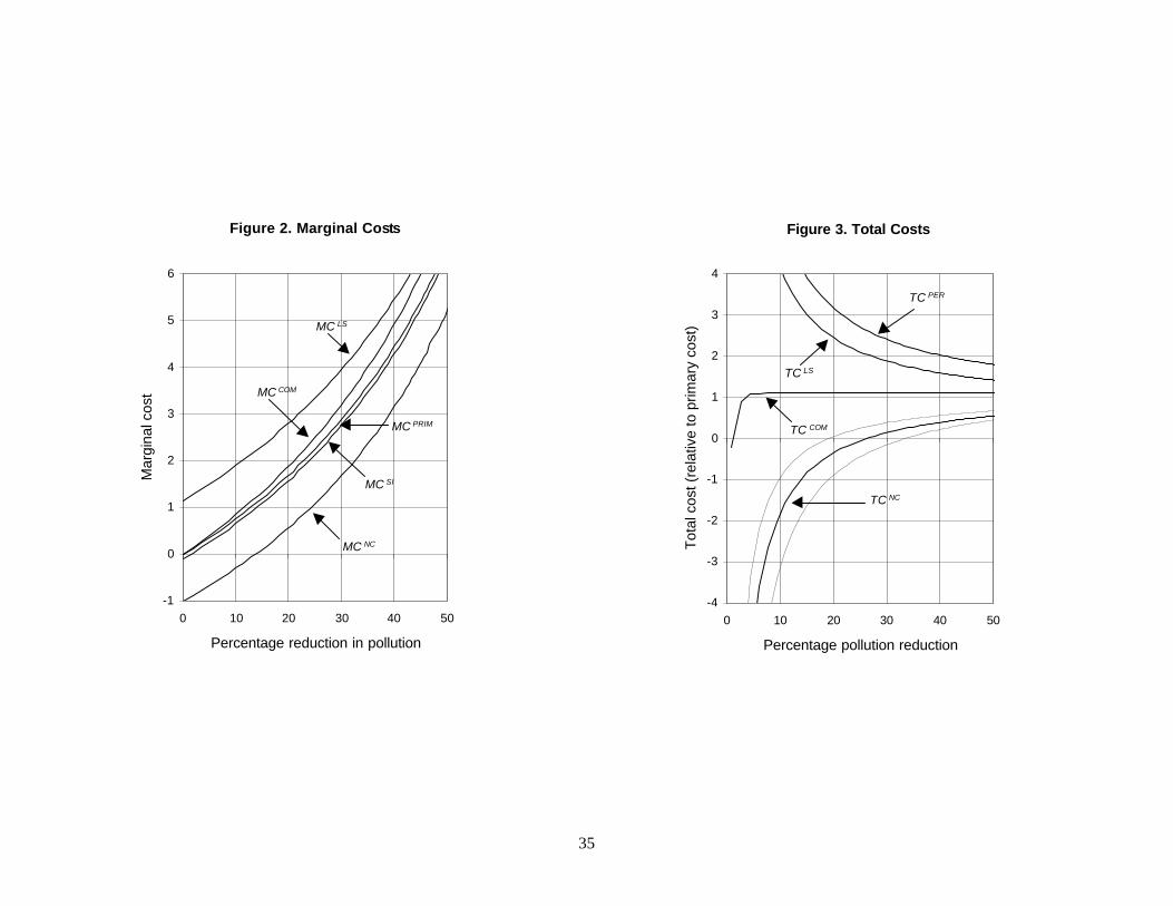
35
Figure 2. Marginal Costs
-1
0
1
2
3
4
5
6
0 10 20 30 40 50
Percentage reduction in pollution
Mar
gina
l cos
t
MC LS
MC COM
MC NC
MC SI
MC PRIM
Figure 3. Total Costs
-4
-3
-2
-1
0
1
2
3
4
0 10 20 30 40 50
Percentage pollution reduction
Tot
al c
ost (
rela
tive
to p
rimar
y co
st)
TC NC
TC PER
TC LS
TC COM

36
Figure 4. Varying the PollutionIntensity of Tax-Favored Consumption
-4
-3
-2
-1
0
1
2
0 0.5 1 1.5 2
Relative pollution intensity of tax-favored consumption
Tot
al c
ost r
atio
for
a 10
per
cent
pol
lutio
n re
duct
ion
TC SI
TC NC
Figure 5. Welfare under the Pigouvian Rule
-4
-3
-2
-1
0
1
2
3
4
0 10 20 30 40 50
Pigouvian pollution reduction
Gen
eral
equ
ilibr
ium
wel
fare
cha
nge
to
Pig
ouvi
an w
elfa
re g
ain
W LS
W NC
W COM

37
Figure 6. Optimal Policies
0
0.3
0.6
0.9
1.2
1.5
1.8
2.1
2.4
0 10 20 30 40 50
Pigouvian pollution reduction
Opt
imal
sec
ond
best
pol
lutio
n re
duct
ion
(re
lativ
e to
Pig
ouvi
an r
educ
tions
)
R COM
R LS
R NC
Related Documents