arXiv:hep-th/0003177v2 5 Apr 2000 March 2000 UMTG–221 hep-th/0003177 Target Space Duality I: General Theory ∗ Orlando Alvarez † Department of Physics University of Miami P.O. Box 248046 Coral Gables, FL 33124 Abstract We develop a systematic framework for studying target space duality at the classical level. We show that target space duality between manifolds M and M arises because of the existence of a very special symplectic manifold. This manifold locally looks like M × M and admits a double fibration. We analyze the local geometric requirements necessary for target space duality and prove that both manifolds must admit flat orthogonal connections. We show how abelian duality, nonabelian duality and Poisson-Lie duality are all special cases of a more general framework. As an example we exhibit new (nonlinear) dualities in the case M = M = R n . PACS: 11.25-w, 03.50-z, 02.40-k Keywords: duality, strings, geometry * This work was supported in part by National Science Foundation grant PHY–9870101. † email: [email protected]

Welcome message from author
This document is posted to help you gain knowledge. Please leave a comment to let me know what you think about it! Share it to your friends and learn new things together.
Transcript
arX
iv:h
ep-t
h/00
0317
7v2
5 A
pr 2
000
March 2000 UMTG–221
hep-th/0003177
Target Space Duality I: General Theory∗
Orlando Alvarez†
Department of Physics
University of Miami
P.O. Box 248046
Coral Gables, FL 33124
Abstract
We develop a systematic framework for studying target space duality at the
classical level. We show that target space duality between manifolds M and
M arises because of the existence of a very special symplectic manifold. This
manifold locally looks like M×M and admits a double fibration. We analyze the
local geometric requirements necessary for target space duality and prove that
both manifolds must admit flat orthogonal connections. We show how abelian
duality, nonabelian duality and Poisson-Lie duality are all special cases of a more
general framework. As an example we exhibit new (nonlinear) dualities in the
case M = M = Rn.
PACS: 11.25-w, 03.50-z, 02.40-k
Keywords: duality, strings, geometry
∗This work was supported in part by National Science Foundation grant PHY–9870101.†email: [email protected]
1 Introduction
The (1 + 1) dimensional sigma model describes the motion of a string on a manifold.
The sigma model is specified by giving a triplet of data (M, g,B) where M is the target
n-dimensional manifold, g is a metric on M , and B is a 2-form on M . The lagrangian
for this model is
L =1
2gij(x)
(∂xi
∂τ
∂xj
∂τ− ∂xi
∂σ
∂xj
∂σ
)+Bij(x)
∂xi
∂τ
∂xj
∂σ(1.1)
with canonical momentum density
πi =∂L∂xi
= gijxj +Bijx
′j , (1.2)
where an overdot denotes the time derivative (∂/∂τ) and a prime denotes the space
derivative (∂/∂σ) on the worldsheet. What is remarkable is that it possible for two com-
pletely different sigma models, (M, g,B) and (M, g, B), to describe the same physics.
By this we mean that there is a canonical transformation between the space of paths on
M and the corresponding one on M that preserves the respective hamiltonians. This
phenomenon is known as target space duality.
This is the first of two articles where we develop a systematic framework for studying
target space duality at the classical level. We do not consider quantum aspects of target
space duality nor do we consider examples involving mirror symmetry. Most of our
considerations are local but phrased in a manner that is amenable to globalization.
We analyze the local geometric requirements necessary for target space duality. The
study of target space duality has developed by discovering a succession of more and
more complicated examples (see below). We show that the known examples of abelian
duality, nonabelian duality and Poisson-Lie duality are all derivable as special cases of
the framework. We show that target space duality boils down to the study of some
very special symplectic manifolds that allow the reduction of the structure group of the
frame bundle to SO(n). In article I we develop the general theory and apply it so some
very simple examples. In article II [1] we systematically apply the theory to a variety
of scenarios and we reproduce nonabelian duality and Poisson-Lie duality. The theory
is applied to other geometric situations that lead us deep into unknown questions in
Lie algebra theory. We try to make article I self contained. References to equations
and sections in article II are preceded by II, e.g., (II-8.3).
What is the value in developing a general framework for studying classical target
space duality? The framework may say something about the what is string theory. We
believe that there is some parameter space that describes string theory. For special
1
values of the parameters we get the familiar Type I, Type II-A, Type II-B, etc. theories
and that these are related by various dualities. If we can get a handle on the class of
symplectic manifolds that lead to target space duality we may be able to get a better
idea about the parameter space of string theory.
The simplest target space duality is abelian duality. Here a theory with target space
S1 or R is dual to a theory with target space S1 or R. For a comprehensive review
and history of abelian duality look in [2]. It should also be mentioned that it has
been known for a long time, see e.g. [3], that the abelian duality transformation is a
canonical transformation. A first attempt to generalize abelian duality to groups led to
the pseudochiral model of Zakharov and Mikhailov [4] as a dual to the nonlinear sigma
model. Nappi [5] showed that these models were not equivalent at the quantum level.
The correct dual model was first found by Fridling and Jevicki [6] and Fradkin and
Tseytlin [7] using path integral methods. String theory motivated a renewed interest
in abelian and nonabelian duality [8, 9, 10, 11, 12, 13, 14, 15]. It was shown that
the duality transformation was canonical [16, 17] and these ideas were generalized in
a variety of ways [18, 19, 20, 21, 22]. The form of the generating functions for duality
transformation gave hints that nonabelian duality was associated with the geometry
of the cotangent bundle of the group.
The most intricate target space duality discovered thus far is the Poisson-Lie duality
of Klimcik and Severa [23, 24, 25]. In this example we see a very nontrivial geometrical
structure playing a central role. A Poisson-Lie group G is a Lie group with a Poisson
bracket that is compatible with the group multiplication law. Drinfeld [26] showed
that Poisson-Lie groups are determined by a Lie bialgebra gD = g ⊕ g where g is the
Lie algebra of G and g is the Lie algebra of a Lie group G, See Appendix II-B.1. The
two Lie algebras are coupled together in a very symmetric way. A Lie group GD with
Lie algebra gD is called a Drinfeld double. It should be pointed out that G is also a
Poisson-Lie group. By using a clever argument, Klimcik and Several discovered that
if the metric g and B field on a Poisson-Lie group G was of a special form then there
would be a corresponding metric g and B-field on the group G. Their observations
follow from the symmetric way that G and G enter into the Drinfeld double GD. They
showed that that by writing down a “first order” sigma model on GD they could derive
either the model on G or the model on G by taking an appropriate slice. Here one
explicitly sees that the the target manifold and the target dual manifold are carefully
glued together into a larger space. Klimcik and Severa do not explicitly write down
the duality transformation but they are totally explicit about the metric and B field.
It was Sfetsos [27, 28] who wrote down the duality transformation, verified that it was
a canonical transformation, and constructed the generating function for the canonical
2
transformation, see also [29].
At the time of the work by Klimcik and Severa, the author had been working on a
program to develop a general theory of target space duality, see [30]. In that article I
advocated the use of generating functions of the type (2.2) because they would lead to
a linear relationship1 between (dx/dσ, π) and (dx/dσ, π) that preserved the quadratic
nature of the sigma model hamiltonians. I discussed the geometry which was involved
and explained the role played in this geometry by the hamiltonian density H and the
momentum density P. Explicit formulas relating the geometries of the two manifolds
were not given in that article for the following reason. The formulation I had at the
time involved variables (x, p) where essentially π = dp/dσ. This gave a certain sym-
metry to some of the equations but at a major price. The B field gauge symmetry
B → B+dA became a nonlocal symmetry in (x, p) space and the gauge symmetry was
no longer manifest. Only for special choices of A was the gauge transformation local.
The formulas I had derived respected the special gauge transformations but I could not
verify general gauge invariance. Sfetsos [27] exploited some of the geometric constraints
I had proposed and he was able to explicitly construct the duality transformation for
Poisson-Lie duality. Sfetsos’ work is very interesting. He conjectures the form of the
duality transformation and he knows the geometric data (M, g,B) and (M, g, B) from
the work of Klimcik and Severa. He now uses this information and certain integrability
constraints to explicitly work out the generating function for the canonical transfor-
mation. Sfetsos’ computation may be reinterpreted as the construction of a known
symplectic structure [32, 33] on the Drinfeld double, see Section II-3.
In this article I present a general theory for target space duality that is manifestly
gauge invariant with respect to B field gauge transformations. I consider what could be
called irreducible duality where there are no spectator fields. All the fields participate
actively in the duality transformation. I show that the duality transformation arises
because of the existence of a special symplectic manifold P that locally looks likeM×Mand admits a double fibration. The duality transformation exists only when there
exists a compatible confluence of several distinct geometric structures associated to the
manifold P : an O(2n) structure related to the hamiltonian density (3.1), an O(n, n)
structure related to the momentum density (3.2), an O(n)×O(n) structure associated
with the sigma model metrics, and a Sp(2n) structure related to the symplectic form.
This is why these symplectic manifolds are very special and rare. I develop the general
theory and then show how the known examples of abelian duality, nonabelian duality
and Poisson-Lie duality follow. The general theory indicates that there are probably
1For nonpolynomial generating functions look at [31].
3
many more examples. For example, in Section 8.3 I write down families of nonlinear
duality transformations that map a theory with target space Rn into one with target
space Rn. I also investigate a variety of scenarios and pose open mathematical questions
deeply related to the theory of Lie algebras.
This work differs from the work of Sfetsos [27] in a variety of ways. There are two
types of constraints on the canonical transformation: algebraic constraints having to
do with quadratic form of the hamiltonian density and differential constraints having
to do integrability conditions. Sfetsos writes these down but in a way that is neither
geometric nor gauge invariant. He applies them to Poisson-Lie duality and derives the
generating function. Sfetsos’ formulation does not exploit the fact that there are natural
geometric structures associated to these equations. This is what I was trying to do in
[30] but failed due to a bad choice of variables (x, p) leading to an absence of manifest
B field gauge invariance. The formulation presented here uses the variables (x, π) and
is manifestly gauge invariant. In Section II-2.2.2 I give a geometric interpretation of
B field gauge invariance. In this article I work in terms of adapted frame fields. In
this way, the formalism has an immediate interpretation in terms of H-structures on
the bundle of frames. In fact the discussion presented in Section II-4.1 is done in a
sub-bundle of the bundle of frames.
The framework developed in this work allows one to attack a variety of interesting
questions. Are there any interesting restrictions on the manifolds M and M? We show
in Section 6 that the manifoldsM and M have to admit flat orthogonal connections. We
know for any manifold M there always exists a natural symplectic manifold P = T ∗M ,
the cotangent bundle. We can ask what type of dualities arises from the standard
symplectic structure on the cotangent bundle? We show that this can only happen if
M is a Lie group, see Section II-2.2.1. This formalism allows general question to be
asked. For example there are a series of PDEs that have to be solved to determine the
duality transformations. These PDEs depend on some functions. If these functions are
zero then one gets abelian duality, if some are made nonzero then you get nonabelian
duality, etc. This is a framework that can be used for a systematic study of duality. It
opens up the possibility to study dualities involving parallelizable manifolds that are
not Lie groups such as S7 or sub-bundles of the frame bundle. This work indicates that
duality is a very rich geometrical framework ripe for study and we have only scratched
the surface.
4
2 The symplectic structure
We review briefly the notion of a “generating function” in canonical transformations
because our methods introduce a secondary symplectic structure into the formulation
of target space duality and it is important to understand the difference between the
two.
Assume you have symplectic manifolds, P and P , with respective symplectic forms
ω and ω. Consider P × P with standard projections Π : P × P → P and Π : P × P →P . You can make P × P into a symplectic manifold by choosing as symplectic form
Ω = Π∗ω − Π∗ω. By definition, a canonical or symplectic transformation f : P → P
satisfies f ∗ω = ω. We describe f by its graph Γf ⊂ P × P . It is clear f : P → P will
be symplectic if and only if Ω|Γf= 0. Locally we have ω = dθ and ω = dθ. Thus we
see that θ − θ is a closed 1-form on Γf . Consequently there exists locally a function
F : Γf → R such that θ − θ = dF . This function F is called the “generating function”
for the symplectic transformation. The reason is that if in local Darboux coordinates
we have that θ = pdq and θ = pdq then we have that F is locally a function of only
q and q, p = ∂F/∂q and p = −∂F/∂q. We can now use the inverse function theorem
to construct the map from (q, p) to (q, p). Note that dim Γf = 2n and therefore F is
a function of 2n variables. Had we chosen θ = −qdp then we would have that F is
a function of q and p. In this case it is worthwhile to observe F = qp generates the
identity transformation. We mention this because the identity transformation is not
in the class of transformations generated by functions of q and q.
All this generalizes to field theory. We discuss only the case of (1 + 1) dimensions.
Let P (M) be the path space of M. By this we mean the set of maps γ : N →M where
N can be R, S1 or [0, π] depending on whether we are discussing infinite strings, closed
strings or open strings. Most of the discussion in this article is local and so we do not
specify N . In the case of a sigma model with target space M , the basic configuration
space is P (M) with associated phase space P (T ∗M). If (x, π) are coordinates on T ∗M
then the symplectic structure on P (T ∗M) is given by∫δπ(σ) ∧ δx(σ) dσ . (2.1)
In what follows we are interested in looking for canonical transformations between a
sigma model with target space M and one with target space M of the same dimension-
ality. We say that a sigma model with geometrical data (M, g,B) is dual to a sigma
model (M, g, B) if there exists a canonical transformation F : P (T ∗M) → P (T ∗M)
that preserves the hamiltonian densities, F ∗H = H, where the hamiltonian density is
given by (3.1).
5
In the case of “abelian duality” where the target space is a circle you can choose
the generating function to be
F [x, x] =
∫xdx
dσdσ .
This leads to the standard duality relations π(σ) = dx/dσ and π(σ) = dx/dσ.
The nonabelian duality relations follow from the following natural choice [20, 22]
for generating function. Assume the target space is a simple connected compact Lie
group G with Lie algebra g. The dual manifold is the Lie algebra with an unusual
metric. The generating function is very natural:
F [g, X] =
∫Tr
(X g−1 dg
dσ
)dσ ,
where X is a Lie algebra valued field.
We now consider a class of generating functions for target space duality that leads
to a linear relationship [30] between (dx/dσ, π(σ)) and the corresponding variables on
the dual space. On M × M choose locally a 1-form α = αi(x, x)dxi + αi(x, x)dx
i. We
can define a natural “generating function” on P (M × M) by
F [x(σ), x(σ)] =
∫α =
∫ (αi(x(σ), x(σ))
dxi
dσ+ αi(x(σ), x(σ))
dxi
dσ
)dσ . (2.2)
We only consider target space duality that arises from this type of canonical transfor-
mation.
Let v be a vector field along the path (x(σ), x(σ)) ∈M × M with compact support
which represents a deformation of the path. Note that δvF =∫Lvα =
∫ιvdα. In
the previous formula Lvα = ιvdα + dιvα is the Lie derivative with respect to v. Since
v has compact support, the exact term can be neglected. Thus the variation of F is
determined by the exact 2-form β = dα:
δvF =
∫ιvβ . (2.3)
We use β to construct the duality transformation. If x and x are respectively local
coordinates on M and M then
β = −1
2lij(x, x)dx
i ∧ dxj +mij(x, x)dxi ∧ dxj +
1
2lij(x, x)dx
i ∧ dxj , (2.4)
where l: lij = −lji and lij = −lji. The three n × n matrix functions l, l, m are used
to construct the canonical transformation on the infinite dimensional phase space. A
6
brief calculation shows that the canonical transformations are
πi(σ) = mji(x, x)dxj
dσ+ lij(x, x)
dxj
dσ, (2.5)
πi(σ) = mij(x, x)dxj
dσ+ lij(x, x)
dxj
dσ. (2.6)
The invertibility of the canonical transformation between P (T ∗M) and P (T ∗M) re-
quires m to be an invertible matrix. This implies that β is of maximal rank, i.e. a
symplectic form2 on M × M .
It is important to recognize that there are two very different symplectic structures
in this problem. The first one is the standard symplectic structure on phase space
P (T ∗M) given by (2.1). The second one on M × M given by β arises from the class
of generating functions (2.2) we are considering. The generating function arguments
are local and suggest that the symplectic structure on M × M may be generalized to
a symplectic manifold P which “contains” M × M . In the cartesian product M × M
you have natural cartesian projections Πc : M × M → M and Πc : M × M → M .
The product structure can be generalized by the introduction of the concept of a
bifibration. A 2n dimensional manifold P is said to be a bifibration if there exists
n dimensional manifolds M and M and projections Π : P → M and Π : P → M
such that the respective fibers are diffeomorphic to coverings spaces of M and M and
they are also transverse. This means that if p ∈ P then ker Π∗|p ⊕ ker Π∗|p = TpP
where Π∗ and Π∗ are the differential maps of the projections. Note that the cartesian
product manifold P = M ×M is an example of a bifibration. If the product projection
Π× Π : P →M ×M is injective3 then P = M ×M . A covering space example is given
by P = R2 and M = M = S1 with Π : (x, x) 7→ eix and Π : (x, x) 7→ eix.
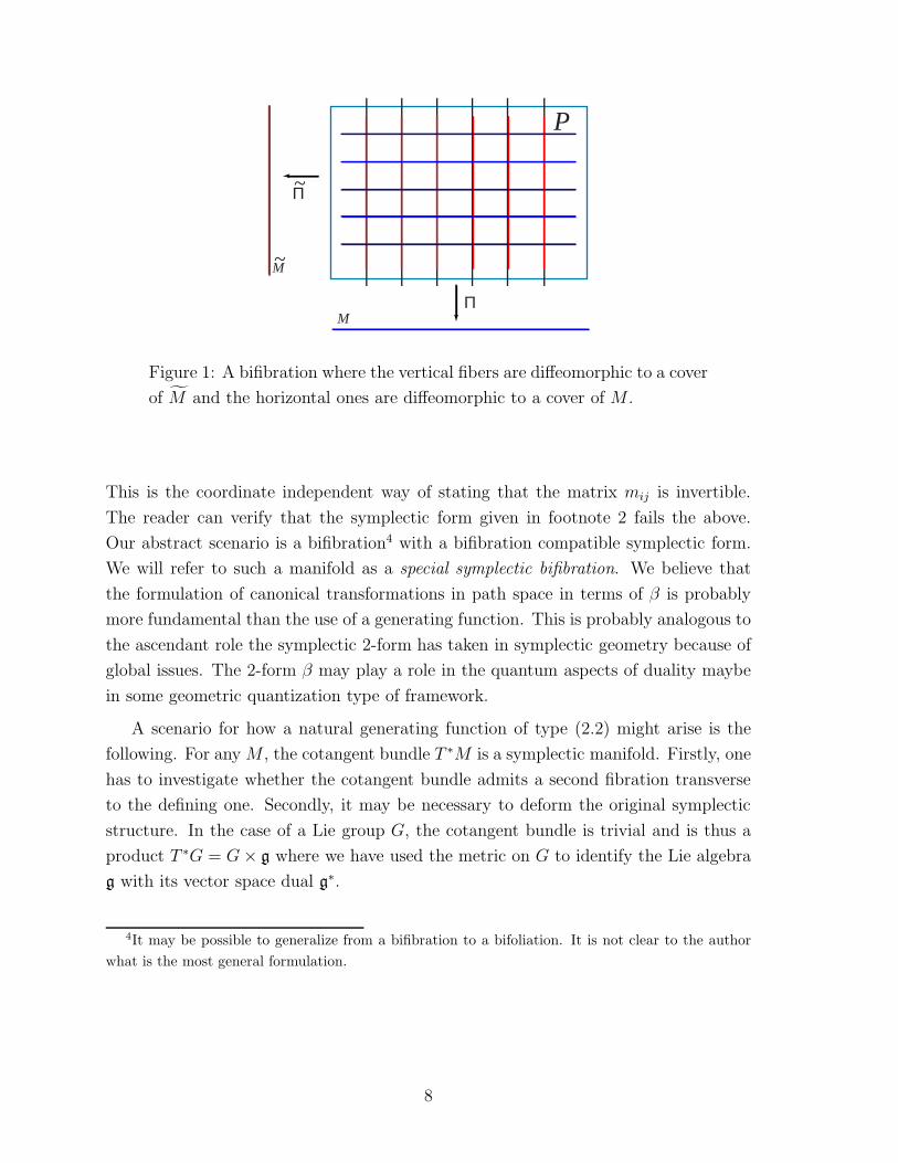
We introduce the following terminology illustrated in Figure 1. At a point p ∈ P
we have a splitting of the tangent space TpP = Hp ⊕ Vp where the “horizontal tangent
space” Hp is tangent to the fiber of Π, and the “vertical tangent space” Vp is tangent
to the fiber of Π. A symplectic form β is said to be bifibration compatible if for every
p ∈ P one has the following nondegeneracy conditions:
1. Given Y ∈ Vp, if for all X ∈ Hp one has β(X, Y ) = 0 then Y = 0.
2. Given X ∈ Hp, if for all Y ∈ Vp one has β(X, Y ) = 0 then X = 0.
2 It is possible for β to be symplectic and have m = 0 but this will not define an invertible canonical
transformation between P (T ∗M) and P (T ∗M). For example, if M and M are symplectic manifolds
with respective symplectic forms ω and ω then choose β = ω − ω.3The definition of a fiber bundle implies that Π × Π is surjective.
7
M
M~
Π
Π~
P
Figure 1: A bifibration where the vertical fibers are diffeomorphic to a cover
of M and the horizontal ones are diffeomorphic to a cover of M .
This is the coordinate independent way of stating that the matrix mij is invertible.
The reader can verify that the symplectic form given in footnote 2 fails the above.
Our abstract scenario is a bifibration4 with a bifibration compatible symplectic form.
We will refer to such a manifold as a special symplectic bifibration. We believe that
the formulation of canonical transformations in path space in terms of β is probably
more fundamental than the use of a generating function. This is probably analogous to
the ascendant role the symplectic 2-form has taken in symplectic geometry because of
global issues. The 2-form β may play a role in the quantum aspects of duality maybe
in some geometric quantization type of framework.
A scenario for how a natural generating function of type (2.2) might arise is the
following. For any M , the cotangent bundle T ∗M is a symplectic manifold. Firstly, one
has to investigate whether the cotangent bundle admits a second fibration transverse
to the defining one. Secondly, it may be necessary to deform the original symplectic
structure. In the case of a Lie group G, the cotangent bundle is trivial and is thus a
product T ∗G = G× g where we have used the metric on G to identify the Lie algebra
g with its vector space dual g∗.
4It may be possible to generalize from a bifibration to a bifoliation. It is not clear to the author
what is the most general formulation.
8
3 Hamiltonian structure
The discussion in the Section 2 is general and makes no reference to the hamiltonian.
The hamiltonian only played an indirect role because we chose a class of canonical
transformations which are linear with respect to dx/dσ and π(σ) in anticipation of
future application to the nonlinear sigma model. The nonlinear sigma model has target
space a riemannian manifold M with metric g and a 2-form field B. The hamiltonian
density and the momentum density are respectively given by
H =1
2gij(x)
(πi − Bik
dxk
dσ
)(πj − Bjl
dxl
dσ
)+
1
2gij(x)
dxi
dσ
dxj
dσ, (3.1)
P = πi(σ)dxi
dσ. (3.2)
We are interested whether we can find a canonical transformation with generating
function of type (2.2) which will map the hamiltonian density and momentum density
into that of another sigma model (the dual sigma model) characterized by target space
M , metric tensor g and 2-form B.
It winds up that working in coordinates is not the best way of attacking the problem.
It is best to use moving frames a la Cartan and Chern. Let (θ1, . . . , θn) be a local
orthonormal coframe5 for M . The Cartan structural equations are
dθi = −ωij ∧ θj ,
dωij = −ωik ∧ ωkj +1
2Rijklθ
k ∧ θl ,
where ωij = −ωji is the riemannian connection6. Next we define dx/dσ in the orthonor-
mal frame to be xσ by requiring that θi = xiσdσ. If π is now the canonical momentum
density in the orthonormal frame then in this frame (3.1) and (3.2) become
H =1
2(πi −Bikx
kσ)(πi −Bilx
lσ) +
1
2xi
σxiσ , (3.3)
P = πixiσ = (πi − Bijx
jσ)xi
σ . (3.4)
In this coframe we can write (2.4) as
β = −1
2lij(x, x)θ
i ∧ θj +mij(x, x)θi ∧ θj +
1
2lij(x, x)θ
i ∧ θj . (3.5)
5Because we will be working in orthonormal frames we do not distinguish an upper index from a
lower index in a tensor.6The riemannian connection is the unique torsion free metric compatible connection. A metric
compatible connection will also be referred to as an orthogonal connection. In general an orthogonal
connection can have torsion.
9
We use the same letters l,m, l but the meaning above is different from (2.4). In this
notation equations (2.5) and (2.6) become
πi(σ) = mji(x, x)xjσ + lij(x, x)x
jσ , (3.6)
πi(σ) = mij(x, x)xjσ + lij(x, x)x
jσ , (3.7)
In matrix notation the above may be written as
(mt 0
−l I
)(xσ
π
)=
(−l I
m 0
)(xσ
π
)
Rewrite the above in the form(
mt 0
−n I
)(xσ
π − Bxσ
)=
(−n I
m 0
)(xσ
π − Bxσ
),
where
n = l −B , (3.8)
n = l − B . (3.9)
The rewriting above is closely related to (A.2), see below. This equation is not very
interesting in this form but it becomes much more interesting when rewritten as
(xσ
π − Bxσ
)=
(mt 0
−n I
)−1(−n I
m 0
)(xσ
π − Bxσ
)
=
(−(mt)−1n (mt)−1
−n(mt)−1n+m n(mt)−1
)(xσ
π − Bxσ
). (3.10)
Notice that equation (3.10) gives us a linear transformation between (xσ, π − Bxσ)
and (xσ, π− Bxσ). The preservation of the hamiltonian density means that this linear
transformation must be in O(2n). If in addition you want to preserve the momentum
density then this transformation must be in OQ(n, n), the group of 2n × 2n matrices
isomorphic to O(n, n) which preserves the quadratic form
Q =
(0 In
In 0
). (3.11)
In the formula above, In is the n × n identity matrix. Properties of OQ(n, n) and its
relation with O(2n) are reviewed in Appendix A. They key observation7 is that the
7I do not understand geometrically why β automatically induces this pseudo-orthogonal matrix.
10
matrix appearing in (3.10) is automatically in OQ(n, n) which means that our canonical
transformation automatically preserves the canonical momentum density (3.4). As
previously mentioned to preserve the hamiltonian density (3.3) is it necessary that the
matrix above also be in O(2n). Thus the matrix(
−(mt)−1n (mt)−1
−n(mt)−1n +m n(mt)−1
)(3.12)
must be in O(2n) ∩OQ(n, n), a compact group locally isomorphic to O(n)×O(n), see
Appendix A. Using the equations in the appendix we learn that the condition that
(3.12) be in the intersection O(2n) ∩ OQ(n, n) is that
mmt = I − n2 , (3.13)
mtm = I − n2 , (3.14)
−mn = nm . (3.15)
We can now simplify (3.12) to(
−(mt)−1n (mt)−1
(mt)−1 −(mt)−1n
)(3.16)
To better understand the above is is worthwhile using the conjugation operation
(A.4) and switch the quadratic from from Q to(
−I 0
0 +I
).
Under this conjugation operation (3.10) becomes(xσ − (π − Bxσ)
xσ + (π − Bxσ)
)
=
(−(mt)−1(I + n) 0
0 (mt)−1(I − n)
)(xσ − (π −Bxσ)
xσ + (π − Bxσ)
). (3.17)
This leads to the pair of equations
(π − Bxσ) + xσ = +T+ [(π − Bxσ) + xσ] , (3.18)
(π − Bxσ) − xσ = −T− [(π − Bxσ) − xσ] , (3.19)
where
T± = (mt)−1(I ∓ n) ∈ O(n) . (3.20)
11
An equivalent way of writing the above is m = T±(I ± n). Also note that T+ and
T− are not independent. They are related by T−1− T+ = (I + n)−1(I − n) which is the
Cayley transform of n. It is often convenient to think that (3.5) is determined by two
orthogonal matrices T± ∈ O(n) with
n = −(T+ + T−)−1(T+ − T−). (3.21)
4 Gauge invariance
It is well known that the sigma model (M, g,B) has a gauge invariance given by B →B + dA where A is a 1-form on M . We can manifest these gauge transformations
within the class (3.20) of canonical transformation by considering∫α →
∫(α + A)
which transforms π appropriately. An observation and a change of viewpoint will
give us a manifestly gauge invariant formulation. Notice that both the left hand side
and right hand side of equation (3.17) is manifestly gauge invariant. This suggests
that m,n, n may be gauge invariant. Looking at (3.8) and (3.9) and incorporating
the remark about how we implement gauge invariance we see that n and n are gauge
invariant quantities, i.e., the gauge transformations are implemented by shifting l, l
respectively by dA and dA. This suggest that instead of working with β it may be
worthwhile to work with γ defined by
γ = −1
2nij(x, x)θ
i ∧ θj +mij(x, x)θi ∧ θj +
1
2nij(x, x)θ
i ∧ θj (4.1)
where γ is not closed but satisfies
dγ = H − H (4.2)
where H = dB and H = dB. More correctly one has dγ = Π∗H − Π∗H . We have now
achieved a gauge invariant formulation.
5 The geometry of P
To gain further insight into relations between the geometry of M and M is it best to
work in P which you may think of it locally being M × M . We can use the freedom of
working in P to simplify results and then project back to either M or M .
There are two closely related ways of simplifying the geometry. One way is to work
in the bundle of orthonormal frames. The other is to adapt the orthonormal frames to
12
the problem at hand similar to the way one uses Darboux frames to study surfaces in
classical differential geometry. The former gives a global formulation but the latter is
more familiar to physicists hence we choose the latter. All our computations will be
local and can be patched together to define global objects.
The first thing to observe is that the existence of the double fibration allows us
to naturally define a riemannian metric on P by pulling back the metrics on M and
M and declaring that the fibers are orthogonal to each other. In a similar fashion
we pullback local coframes and get local coframes on P . These orthonormal coframes
satisfy the Cartan structural equations
dθi = −ωij ∧ θj , (5.1)
dθi = −ωij ∧ θj , (5.2)
dωij = −ωik ∧ ωkj +1
2Rijklθ
k ∧ θl , (5.3)
dωij = −ωik ∧ ωkj +1
2Rijklθ
k ∧ θl . (5.4)
Once we begin working on P then we have the freedom to independently rotate θ and
θ at each point. Once we do this these coframes will no longer be pullbacks but this
doesn’t matter because it does not change the metric on each fiber. We are going to
exploit this freedom to relate the geometry of M to that of M in a way similar to the
way the intrinsic curvature of a submanifold is related to the total curvature of the
space and the curvature of the normal bundle. Note that with these choices there is a
natural group of O(n)×O(n) gauge transformations on the tangent bundle of P which
is compatible with the metric structure and the bifibration.
6 Constraints from the algebraic structure of γ
First we derive various constraints that follow from the algebraic constraints on γ
imposed by the preservation of H and P. Equations (3.14) and (3.15) tell us that
m = T (I + n) and n = −TnT t (6.1)
where T ∈ O(n). Since T “connects” a θ to a θ we see that its covariant differential is
given by
dTij + ωikTkj + ωjkTik = +Tijkθk − Tijkθ
k , (6.2)
where the components of the covariant differential in the M direction is +Tijk and
in the M direction is −Tijk. The negative sign is introduced for future convenience.
13
Notice that Tijk and Tijk are tensors defined on P whose existence is guaranteed by
the existence of the tensor Tij on P .
We now invoke a “symmetry breaking mechanism” to reduce the structure group of
gauge transformations from O(n)×O(n) to O(n). At each point in P we can rotate θ
(or θ) and make T = I because under these gauge transformations T → RTR−1 where
(R, R) ∈ O(n) × O(n). The isotropy group of T = I is the diagonal O(n). This is no
different than giving a scalar field a vacuum expectation value to break the symmetry.
This symmetry breaking leads to an identification at each point of P of the “vertical”
and “horizontal” tangent spaces. This does not tell us that the metrics are the same
but allows us to identify an orthonormal frame in one with an orthonormal frame in the
other. Let us be a bit more precise and abstract on the reduction of the structure group
and the identification of the “vertical” and “horizontal” tangent spaces. We already
mentioned that at p ∈ P one has TpP = Hp ⊕ Vp. The tensor m(p) may be viewed as
an element of V ∗p ⊗H∗
p . Because there is a metric on Vp we can reinterpret m as giving
us an invertible linear transformation m : Hp → Vp. We also have a metric on Hp and
thus we can study the orbit of m(p) under the action of O(n) × O(n). Our previous
discussion shows that a “canonical” form for m(p) may be taken to be m(p) = I+n(p)
with isotropy group being the diagonal O(n). If (e1, . . . , en) is an orthonormal basis at
Hp and (e1, . . . , en) is the corresponding orthonormal basis at Vp then they are related
by m(p)ei = ej(δji + nji(p)).
From now on we assume we have adapted our coframes such that T = I and
mij = δij + nij , (6.3)
nij = nij . (6.4)
In this frame, γ simplifies to
γ = θi ∧ θi + nij θi ∧ θj − 1
2nijθ
i ∧ θj − 1
2nij θ
i ∧ θj . (6.5)
The duality equations are particularly simple now and they are given by
(π − Bxσ) + xσ = (π −Bxσ) + xσ , (6.6)
(π − Bxσ) − xσ = −T− [(π − Bxσ) − xσ] , (6.7)
Where the orthogonal matrix T− is the Cayley transform of n:
T− =I + n
I − n. (6.8)
The matrix T− is not arbitrary because there are constraints on nij as we will see later
on. Without constraints on T− there are interesting solutions to (6.6) and (6.7) which
14
map spaces of constant positive curvature into spaces of negative constant curvature
or more generally dual symmetric spaces8.
We can now exploit equation (6.2) to relate the connections in the adapted cofram-
ing. Inserting T = I into the above leads to
ωij − ωij = +Tijkθk − Tijkθ
k . (6.9)
Thus we see that in the reduction of the structure group we have generated torsion and
that this torsion satisfies Tijk = −Tjik and Tijk = −Tjik. We now define an orthogonal
connection on our adapted frames by
ψij = ωij + Tijkθk = ωij + Tijkθ
k . (6.10)
First we define the components of the covariant derivatives of T and T by
dTijk + (ω · T )ijk = T ′ijklθ
l + T ′′ijklθ
l , (6.11)
dTijk + (ω · T )ijk = T ′ijklθ
l + T ′′ijklθ
l . (6.12)
In the above (ω · T ) and (ω · T ) are abbreviations for standard expressions. We have
chosen to use the connections ω and ω rather than ψ in the definition of the covariant
derivative for the following reasons: if Tijk is the pullback of a tensor on M then
T ′′ijkl = 0; if Tijk is the pullback of a tensor on M then T ′
ijkl = 0. A notational remark is
that a primed tensor denoted the covariant derivative in the M direction and a doubly
primed tensor denotes the covariant derivative in the M direction. Doubly primed does
not mean second derivative.
The curvature of this connection may be computed by either using the expression
involving ω or the one involving ω. A straightforward computation of the curvature
matrix 2-form
Ψij = dψij + ψik ∧ ψkj (6.13)
in these two ways leads to the following expressions
Ψij = −T ′′ijlmθ
l ∧ θm
+1
2
[Rijlm − (T ′
ijlm − T ′ijml) + (TiklTkjm − TikmTkjl)
]θl ∧ θm ,
and
Ψij = −T ′ijlmθ
l ∧ θm
+1
2
[Rijlm − (T ′′
ijlm − T ′′ijml) + (TiklTkjm − TikmTkjl)
]θl ∧ θm .
8O. Alvarez, unpublished.
15
Comparing these two expression we learn that the curvature two form matrix is given
by
Ψij = dψij + ψik ∧ ψkj = −T ′′ijlmθ
l ∧ θm . (6.14)
The following constraints must also hold
Rijlm − (T ′ijlm − T ′
ijml) + (TiklTkjm − TikmTkjl) = 0 , (6.15)
Rijlm − (T ′′ijlm − T ′′
ijml) + (TiklTkjm − TikmTkjl) = 0 , (6.16)
T ′′ijlm + T ′
ijml = 0 . (6.17)
Form (6.14) is reminiscent of a Kahler manifold where the curvature is of type dz ∧ dzand there are no dz ∧ dz or dz ∧ dz components. The absence of these many curvature
components is due to the reduction of the structure group from O(2n) to O(n) at the
expense of generating torsion.
There are a variety of equivalent ways of interpreting the above. The most geometric
is to observe that ψij defines a connection on P and thus a connection when restricted
to any of the fibers. For example, let Mx = Π−1(x) be a horizontal fiber. Notice that
along this fiber θ = 0 and thus Ψij = 0. Since Mx is isometric to M we have found
a flat orthogonal connection (generally with torsion) on M . Note that this is true for
all horizontal fibers. One can make a similar statement about the vertical fibers. We
have our first major result.
Target space duality requires that the manifolds M and M respectively admit
flat orthogonal connections. The connection ψij is flat when restricted to
either M or M .
At a more algebraic level equations (6.15) and (6.16) are the standard equations for
“parallelizing” the curvature by torsion. A manifold M is said to be parallelizable if
the tangent bundle is a product bundle TM = M × Rn. This means that you can
globally choose a frame on M . The existence of a flat connection on a manifold does
not imply parallelizability. The reason is that in a non-simply connected manifold there
is an obstruction to globally choosing a frame if there is holonomy. If the manifold
is simply connected and the connection is flat then it is parallelizable. Finally we
observe that if a manifold is parallelizable then there are an infinite number of other
possible parallelizations9. Assume we have an orthogonal parallelization, i.e., a choice
of orthonormal frame at each point. Given any other orthogonal parallelization we can
9I would like to thank I.M. Singer for the ensuing argument.
16
always make a rotation point by point so that both frames agree at the point. Thus
the space of all orthogonal parallelizations is given by the set of maps from M to O(n).
Note that given two distinct points x1, x2 ∈ M , the tensor Tijk on the respective
horizontal fibers Mx1and Mx2
do not have to be the same. There are many flat
orthogonal connections on M as can be seen by a variant parallelizability argument.
In fact you could in principle have a multiparameter family parametrized by M .
There is a special case of interest when Tijk is the pullback of a tensor on M . In
this case a previous remark tells us that T ′′ijkl = 0 and consequently by (6.17) we also
have T ′ijkl = 0. Therefore Tijk is also the pullback of a tensor on M . This means that
the same torsion tensors make the connection flat on all the fibers. Note that in this
case Ψij = 0 and the orthogonal connection ψij is a flat connection on P .
If Tijk is the pullback of a tensor on M then Tijk is the pullback of a tensor
on M and Ψij = 0. In this case ψij is a flat connection on P .
7 Simple examples
The equation dγ = H − H introduces relations among H, H, Tijk and Tijk. First we
point out some facts.
7.1 The case of nij = 0
As a warmup we study the case where nij = 0. In this case γ = θi∧θi and we compute
dγ by using the Cartan structural equations (5.1), (5.2) and the condition which follows
from the reduction of the symmetry group (6.9). A brief computation yields
dγ = Tkijθi ∧ θj ∧ θk − Tijkθ
i ∧ θj ∧ θk .
First we learn that the 3-forms H and H vanish. Next we see that Tkij = Tkji and
Tijk = Tikj. We remind the reader that a tensor Sijk which is skew symmetric under
i ↔ j and symmetric under j ↔ k is zero. Thus we conclude that Tijk = Tijk = 0. It
follows from equations (6.15) and (6.16) that Rijkl = Rijkl = 0. Since the Riemannian
curvatures vanish we know thatM and M are manifolds with universal cover Rn. There
are no other possibilities if nij = 0. For example you can have M = Tk × R
n−k. This
is the case of abelian duality. Other potential singular cases of interest are orbifolds or
cones which are flat but have holonomy due to the presence of singularities.
17
7.2 The case of a Lie group
We verify that the standard nonabelian duality results are reproducible in this formal-
ism. We present a schematic discussion here because the Lie group example is a special
case of a more general result presented in Section II-2.2.1. Let G a compact simple Lie
group with Lie algebra g. Let (ei, . . . , en) is an orthonormal basis for g with respect
to the Killing form. The structure constants fijk are defined by [ei, ej] = fkijek. In
this case the structure constants are totally antisymmetric. Let θi be the associated
Maurer-Cartan forms satisfying the Maurer-Cartan equations
dθi = −1
2fijkθ
j ∧ θk . (7.1)
Because of the Killing form we can identify the Lie algebra g with its vector space
dual g∗. We choose P to be the cotangent bundle T ∗G which is a product bundle
T ∗G = G× g∗ = G× g. If (p1, . . . , pn) are the standard coordinates on the cotangent
bundle with respect to the orthonormal frame then the we take α in (2.2) to be α = piθi,
the canonical 1-form on T ∗G. Therefore β = dα is the standard symplectic form on
T ∗G given by
β = dpi ∧ θi − 1
2pifijkθ
j ∧ θk . (7.2)
By looking at reference [22] one can see that the orthonormal coframe (θ1, . . . , θn) on
the fiber g∗ is given by dpj = θi(δij + fkijpk). This suggests that mij = (δij + fkijpk)
and that in this basis the symmetry breaking is manifest and thus nij = fkijpk. Thus
we expect that γ is given by
γ = −1
2fkijpkθ
i ∧ θj + (δij + fkijpk)θi ∧ θj − 1
2fkijpkθ
i ∧ θj . (7.3)
Note that dγ = −H because the modification of going from the closed form β to γ
involved a term of the type nij θi ∧ θj . To verify this we observe that θi = dpjm
−1ji and
thus nij θi ∧ θj only depends on p and dp, therefore, its exterior derivative can only be
of type dp ∧ dp ∧ dp ∼ θ ∧ θ ∧ θ. In fact 12fkijpkθ
i ∧ θj is the standard representation
for the 2-form B.
If we write dθi = −12fijkθ
j ∧ θk then a straightforward exercise shows that
fijk = (mjmfmkl −mkmfmjl)m−1li .
By using (B.1) one can compute ωij. It is now an algebraic exercise to compute
parallelizing torsions Tijk and Tijk.
18
8 The case of a general connection ψ
8.1 General theory
We already saw that the connection ψij on P gives a flat connection on both M and
M , a necessary condition for M and M to be target space duals of each other. We
are going to take the following approach. Assume we are given a ψij on P , how do we
determine nij? We will derive PDEs that nij must satisfy. If there exist solutions to
these PDEs then we automatically have a duality between the sigma model on M and
the one on M . for It is worthwhile to rewrite the Cartan structural equations in terms
of ψij :
dθi = −ψij ∧ θj − 1
2fijkθ
j ∧ θk , (8.1)
dθi = −ψij ∧ θj − 1
2fijkθ
j ∧ θk , (8.2)
dψij = −ψik ∧ ψkj − T ′′ijlmθ
l ∧ θm . (8.3)
where fijk = −fikj , fijk = −fikj and T ′′ijkl = −T ′′
jikl. The structure functions fijk and
fijk are related to Tijk and Tijk by
fijk = Tijk − Tikj, Tijk =1
2(fijk − fjik − fkij) , (8.4)
fijk = Tijk − Tikj, Tijk =1
2(fijk − fjik − fkij) . (8.5)
We define the components n′ijk, n
′′ijk, f
′ijkl, f
′′ijkl, f
′ijkl, f
′′ijkl of the covariant derivatives of
nij , fijk, fijk with respect to the connection ψij by
dnij + ψiknkj + ψjknik = n′ijkθ
k + n′′ijkθ
k . (8.6)
dfijk + ψilfljk + ψjlfilk + ψklfijl = f ′ijklθ
l + f ′′ijklθ
l , (8.7)
dfijk + ψilfljk + ψjlfilk + ψklfijl = f ′ijklθ
l + f ′′ijklθ
l . (8.8)
There are several important constraints which follow from d2θ = d2θ = 0:
(−f ′
ijkl + fmjkfiml
)θj ∧ θk ∧ θl = 0 , (8.9)
f ′′ijkl = T ′′
ijkl − T ′′ikjl , (8.10)
(−f ′′
ijkl + fmjkfiml
)θj ∧ θk ∧ θl = 0 (8.11)
f ′ijkl = −(T ′′
ijlk − T ′′iklj) . (8.12)
19
Note that T ′′ijkl = 0 if and only if f ′′
ijkl = f ′ijkl = 0, i.e., fijk and fijk are respectively
pullbacks in accord with a previous remark. The d2ψij = 0 constraints are not used in
this report and will not be given.
To derive the PDE satisfied by nij we compute dγ:
dγ = H − H
= −1
2n′
ijkθi ∧ θj ∧ θk +
1
2f ijkn
ilθ
j ∧ θk ∧ θl
− 1
2n′′
ijkθi ∧ θj ∧ θk − n′
ijkθi ∧ θk ∧ θj
+1
2f ijkθ
j ∧ θk ∧ θi − 1
2f ijkn
ilθ
j ∧ θk ∧ θl
+ n′′ijkθ
i ∧ θj ∧ θk − 1
2n′
ijkθk ∧ θi ∧ θj
− 1
2f ijkθ
i ∧ θj ∧ θk − 1
2f ijkn
ilθ
l ∧ θj ∧ θk
− 1
2n′′
ijkθi ∧ θj ∧ θk
+1
2f ijkn
ilθ
j ∧ θk ∧ θl. (8.13)
If we write the closed 3-forms in components as
H =1
3!Hijkθ
i ∧ θj ∧ θk , H =1
3!Hijkθ
i ∧ θj ∧ θk , (8.14)
where Hijk and Hijk are totally skew symmetric then we immediately see that
n′ijk + n′
jki + n′kij = −Hijk + (flijnlk + fljknli + flkinlj) , (8.15)
n′′ijk + n′′
jki + n′′kij = +Hijk + (flijnlk + fljknli + flkinlj) , (8.16)
(n′kij − n′
kji) − n′′ijk = −(fkij − nlkflij) = −mklflij , (8.17)
−n′ijk + (n′′
kij − n′′kji) = +(fkij + nlkflij) = flijmlk . (8.18)
The number of linearly independent equations above is 13n(n − 1)(2n − 1). The best
way to see this is that if we define ξi± = (θi ∓ θi) then the term containing nij in γ is
basically nijξi+ ∧ ξj
+. If the components of the covariant derivatives of nij in this basis
are n±ijk then d(nijξ
i+∧ ξi
+) ∼ n+ijkξ
k+∧ ξi
+ ∧ ξj+ +n−
ijkξk−∧ ξi
+ ∧ ξj+ . . .. The stuff in ellipsis
does not involves derivatives of nij. Since n+ijk is linearly independent of n−
ijk we see
that the number of equations we get is 13!n(n − 1)(n − 2) + n × 1
2n(n − 1). The first
remark we make is that the PDEs given by (8.6) generally make an overdetermined
system if n > 1. The reason is that there are 13n(n−1)(2n−1) equations for 1
2n(n−1)
functions nij . This means that for a solution to exist integrability conditions arising
from d2nij = 0 must be satisfied.
20
Let tijk = −tjik be a tensor in (∧2 V ) ⊗ V for some n dimensional vector space V
with inner product. The vector space (∧2 V ) ⊗ V has an orthogonal decomposition
into (∧3 V ) ⊕ ((
∧2 V ) ⊗ V )mixed where the latter are the tensors of mixed symmetry
under the permutation group. The orthogonal projectors A (antisymmetrization) and
M (mixed) that respectively project onto∧3 V and ((
∧2 V ) ⊗ V )mixed are
(At)ijk =1
3(tijk + tjki + tkij) , (8.19)
(Mt)ijk =1
3(2tijk − tjki − tkij) . (8.20)
A detailed analysis (see below) of equations (8.15), (8.16), (8.17) and (8.18) shows that
they determine An′, An′′ and M(n′ +n′′). These equations do not provide information
about M(n′ − n′′).
To solve the equations above it is best on introduce the following auxiliary tensors:
Vijk = Hijk − (flijnlk + fljknli + flkinlj) , (8.21)
Vijk = Hijk + (flijnlk + fljknli + flkinlj) , (8.22)
Wijk = (fkij − nlkflij) = mklflij , (8.23)
Wijk = (fkij + nlkflij) = flijmlk . (8.24)
They are all skew symmetric under the interchange i ↔ j and V, V are totally anti-
symmetric. Given a value for nij , these tensor are determined by the geometric data
which specifies the sigma models. This data is not independent because these tensors
are linearly related due to the right hand sides of (8.15), (8.16), (8.17) and (8.18).
A little algebra shows that
n′ + n′′ = W − V = −W + V . (8.25)
All the content of (8.15), (8.16), (8.17) and (8.18) is contained in (8.15), (8.16) and
(8.25). These equations place constraints on V, V ,W, W . Immediate conclusions are
that
W + W = V + V , (8.26)
M(W + W ) = 0 , (8.27)
AW =2
3V +
1
3V , (8.28)
AW =1
3V +
2
3V . (8.29)
21
In deriving the last two equation we used (8.15), (8.16) and applied the A operator to
(8.25). The equations above imply linear algebraic relations among the data that de-
fines the sigma models. They tell us that there exists a tensor Uijk of mixed symmetry,
i.e., Uijk = −Ujik and AU = 0 such that
W = +U +2
3V +
1
3V , (8.30)
W = −U +1
3V +
2
3V . (8.31)
Collating all our information we can now write down the 13n(n − 1)(2n − 1) first
order linear PDEs that determine nij:
An′ = −1
3V , (8.32)
An′′ = +1
3V , (8.33)
M(n′ + n′′) = +U . (8.34)
There is no equation for M(n′ − n′′). It is worthwhile to note that
n′ =1
2U +
1
2M(n′ − n′′) − 1
3V , (8.35)
n′′ =1
2U − 1
2M(n′ − n′′) +
1
3V . (8.36)
You can envision using this formalism in four basic scenarios.
1. Test to see if two sigma models (M, g,B) and (M, g, B) are dual to each other.
This entails the construction of the symplectic manifold P .
2. Given a sigma model (M, g,B) and a symplectic manifold P , naturally associated
with M , can you construct the dual sigma model (M, g, B)?
3. Given a symplectic manifold P that admits a bifibration, attempt to construct
dual sigma models.
4. Find all symplectic manifolds P that admit dual sigma models.
8.2 Covariantly constant nij
Here we show that the assumption of covariantly constant nij leads to a flat connection
on P . Assume that in our adapted coframes the nij are covariantly constant with
22
respect to the ψ connection, i.e., n′ijk = n′′
ijk = 0. In this case it is immediate from
(8.17) and (8.18) that fijk = fijk = 0. Subsequently we see from (8.15) and (8.16)
that H = H = 0. From (8.10) we see that T ′′ijkl = 0 and thus the curvature vanishes,
Ψij = 0. We are mostly interested in local properties so we might as well assume P is
parallelizable. We can use parallel transport with respect to this connection to get a
global framing. In this special framing the connection coefficients vanish and thus we
can make the substitution ψij = 0 in all the equations in Section 8.1. Note that the
orthonormal coframes satisfy dθi = dθi = 0 and thus M and M are manifolds with
cover Rn. Following up on remarks made in Section 7.1 we see that this is the case of
abelian duality but with constant nij in the adapted frames corresponding to constant
Bij and Bij .
8.3 Case of fijk = 0.
What is the most general manifold M whose dual M has cover Rn? Note that by
(8.5) we have that Tijk = 0 and thus T ′′ijlm = −T ′
ijml = 0. This means that the
curvature (6.14) of the connection ψij vanishes. Again using the remarks just made
we can choose a parallel framing such that ψij = 0. Since fijk = 0 we have that
dθi = 0 and thus locally there exists functions xi such that θi = dxi. We also have
that dθi = −12fijkθ
j ∧ θk. Previous arguments also tell us that fijk is the pullback of a
tensor on M . From (8.22) we see that V = H and from (8.24) we have that W = 0.
Equation (8.31) tells us that U = 0 and V = −2V = −2H. Inserting into (8.30) we
find that
Wijk = mklflij = (δkl + nkl)flij = −Hijk . (8.37)
An elementary consequence of this equation is that if H = 0 then fijk = 0 and M is
also a manifold with cover Rn. Inserting the above into (8.21) we find that
Hijk = Hijk − (fijk + fjki + fkij) . (8.38)
The left hand side is the pullback of a tensor on M and the right hand side is the
pullback of a tensor on M thus each side must be constant. We have learned that Hijk
are constants. We assume that nij are not constant (see Section 8.2). From (8.37) we
expect the fijk not to be constant. Let µijk be a tensor of mixed symmetry then from
(8.35) and (8.36) we see that
dnkl =
(µklm − 2
3Hklm
)θm +
(−µklm +
1
3Hklm
)θm . (8.39)
The answer to the question, “What is the most general manifold M whose dual M has
cover Rn?” and the construction of the duality transformation is given by the general
23
solution to the following system of exterior differential equations:
(δkl + nkl)dθl =
1
2Hkijθ
i ∧ θj , (8.40)
dθi = 0 , (8.41)
dnkl =
(µklm − 2
3Hklm
)θm +
(−µklm +
1
3Hklm
)θm . (8.42)
As an example consider the special case of H = 0. From (8.37) we have that
fijk = 0. We are now asking, “What is the most general duality transformation between
manifolds with cover Rn?” The equations above tell us that there exists functions xi
and xj such that θi = dxi and θj = dxj . Equation (8.42) becomes dnkl = µklmdym
where yi = xi − xi. We learn that nij is a function of y only. Since the tensor µ has
mixed symmetry we see that d(nij(y)dyi ∧ dyj) = 0 and thus we conclude that locally
there exists functions ri of the independent variables yj such that
1
2nij(y)dy
i ∧ dyj = d(ri(y)dy
i).
We now have all the information required to construct the duality transformation. The
duality transformations are given by
π + xσ = π + xσ ,
π − xσ = −T−(x− x) [π − xσ]
with T−(y) = (I+n(y))(I−n(y))−1. By taking the sum and difference of the equations
above one gets ODEs that can be solved for (x(σ), π(σ)) given (x(σ), π(σ)).
Acknowledgments
I would like to thank O. Babelon, L. Baulieu, T. Curtright, L.A. Ferreira, D. Freed,
S. Kaliman, C-H Liu, R. Nepomechie, N. Reshetikhin, J. Sanchez Guillen, N. Wallach
and P. Windey for discussions on a variety of topics. I would also like to thank Jack Lee
for his Mathematica package Ricci that was used to perform some of the computations.
I am particularly thankful to R. Bryant and I.M. Singer for patiently answering my
many questions about differential geometry. This work was supported in part by
National Science Foundation grant PHY–9870101.
Appendices
24
A Facts about orthogonal groups
We collate some basic properties of orthogonal groups in this section. An orthogonal
matrix in O(n, n) may be written in terms of n× n blocks as
(A B
C D
)
where AtA + CtC = I, BtB + DtD = I and BtA + DtC = 0. A matrix in the Lie
algebra so(n, n) may be written as
(a b
c d
)
where a = −at, d = −dt and c = −bt.The group OQ(n, n) ⊂ GL(2n,R) is defined to be the linear transformations which
leave
Q =
(0 In
In 0
).
invariant. A matrix in OQ(n, n) may be written in n× n blocks as
(W X
Y Z
)(A.1)
where W tZ + Y tX = I, W tY + Y tW = 0 and X tZ + ZtX = 0. It is very important
to observe that matrices of the form(I 0
Y I
)(A.2)
where Y = −Y t are in OQ(n, n). A matrix in the Lie algebra soQ(n, n) may be written
as (w x
y z
)(A.3)
where z = −wt, y = −yt and x = −xt.
Conjugating by the orthogonal matrix
T =1√2
(In −InIn In
)
leads one to the observation that
T
(0 In
In 0
)T−1 =
(−In 0
0 In
). (A.4)
25
Therefore the group OQ(n, n) is isomorphic to O(n, n).
We will also need to identify the compact group O(2n) ∩ OQ(n, n). To do this we
observe that at the Lie algebra level so(2n)∩ soQ(n, n) is given by matrices of the form
(a b
b a
)
where at = −a and bt = −b. Conjugating by T one sees that
T
(a b
b a
)T−1 =
(a− b 0
0 a+ b
).
Therefore, the intersection so(2n) ∩ soQ(n, n) is conjugate to so(n) ⊕ so(n).
B On the structure functions
In a local orthonormal coframe one has the Cartan structural equations (5.1). Locally
one can always write dθi = −12fijkθ
j ∧ θk for some “structure functions” fijk which are
skew symmetric in j ↔ k. If we write the riemannian connection as ωij = ωijkθk then
ωijk =1
2(fkij − fijk + fjik) . (B.1)
This allows us to reconstruct all the local Riemannian geometry of the manifold in
terms of the structure functions.
References
[1] O. Alvarez, “Target space duality II: Applications,” hep-th/0003178.
[2] A. Giveon, M. Porrati, and E. Rabinovici, “Target space duality in string
theory,” Phys. Rept. 244 (1994) 77–202, hep-th/9401139.
[3] A. Giveon, E. Rabinovici, and G. Veneziano, “Duality in string background
space,” Nucl. Phys. B322 (1989) 167.
[4] V. E. Zakharov and A. V. Mikhailov, “Relativistically invariant two-dimensional
models in field theory integrable by the inverse problem technique. (in
Russian),” Sov. Phys. JETP 47 (1978) 1017–1027.
[5] C. R. Nappi, “Some properties of an analog of the nonlinear sigma model,”
Phys. Rev. D21 (1980) 418.
26
[6] B. E. Fridling and A. Jevicki, “Dual representations and ultraviolet divergences
in nonlinear sigma models,” Phys. Lett. B134 (1984) 70.
[7] E. S. Fradkin and A. A. Tseytlin, “Quantum equivalence of dual field theories,”
Ann. Phys. 162 (1985) 31.
[8] E. B. Kiritsis, “Duality in gauged WZW models,” Mod. Phys. Lett. A6 (1991)
2871–2880.
[9] M. Rocek and E. Verlinde, “Duality, quotients, and currents,” Nucl. Phys. B373
(1992) 630–646, hep-th/9110053.
[10] A. Giveon and M. Rocek, “Generalized duality in curved string backgrounds,”
Nucl. Phys. B380 (1992) 128–146, hep-th/9112070.
[11] X. C. de la Ossa and F. Quevedo, “Duality symmetries from nonabelian
isometries in string theory,” Nucl. Phys. B403 (1993) 377–394, hep-th/9210021.
[12] M. Gasperini, R. Ricci, and G. Veneziano, “A problem with nonabelian
duality?,” Phys. Lett. B319 (1993) 438–444, hep-th/9308112.
[13] A. Giveon and M. Rocek, “Introduction to duality,” hep-th/9406178.
[14] A. Giveon and M. Rocek, “On nonabelian duality,” Nucl. Phys. B421 (1994)
173–190, hep-th/9308154.
[15] A. Giveon and E. Kiritsis, “Axial vector duality as a gauge symmetry and
topology change in string theory,” Nucl. Phys. B411 (1994) 487–508,
hep-th/9303016.
[16] T. Curtright and C. Zachos, “Currents, charges, and canonical structure of
pseudodual chiral models,” Phys. Rev. D49 (1994) 5408–5421, hep-th/9401006.
[17] E. Alvarez, L. Alvarez-Gaume, and Y. Lozano, “A canonical approach to duality
transformations,” Phys. Lett. B336 (1994) 183–189, hep-th/9406206.
[18] E. Alvarez, L. Alvarez-Gaume, and Y. Lozano, “On nonabelian duality,” Nucl.
Phys. B424 (1994) 155–183, hep-th/9403155.
[19] E. Alvarez, L. Alvarez-Gaume, J. L. F. Barbon, and Y. Lozano, “Some global
aspects of duality in string theory,” Nucl. Phys. B415 (1994) 71–100,
hep-th/9309039.
27
[20] Y. Lozano, “Nonabelian duality and canonical transformations,” Phys. Lett.
B355 (1995) 165–170, hep-th/9503045.
[21] Y. Lozano, “Duality and canonical transformations,” Mod. Phys. Lett. A11
(1996) 2893–2914, hep-th/9610024.
[22] O. Alvarez and C.-H. Liu, “Target space duality between simple compact lie
groups and lie algebras under the hamiltonian formalism: 1. remnants of duality
at the classical level,” Commun. Math. Phys. 179 (1996) 185, hep-th/9503226.
[23] C. Klimcik and P. Severa, “Dual nonabelian duality and the Drinfeld double,”
Phys. Lett. B351 (1995) 455–462, hep-th/9502122.
[24] C. Klimcik and P. Severa, “Poisson-Lie T-duality and loop groups of Drinfeld
doubles,” Phys. Lett. B372 (1996) 65–71, hep-th/9512040.
[25] C. Klimcik and P. Severa, “Poisson-Lie T-duality: Open strings and d-branes,”
Phys. Lett. B376 (1996) 82–89, hep-th/9512124.
[26] V. I. Drinfeld, “Hamiltonian structures on Lie groups, Lie bialgebras, and the
geometric meaning of the Yang-Baxter equation,” Dokl. Akad. Nauk SSSR 268,2
(1983) 798–820.
[27] K. Sfetsos, “Canonical equivalence of non-isometric sigma-models and
Poisson-Lie T-duality,” Nucl. Phys. B517 (1998) 549–566, hep-th/9710163.
[28] K. Sfetsos, “Poisson-Lie T-duality and supersymmetry,” Nucl. Phys. Proc. Suppl.
56B (1997) 302, hep-th/9611199.
[29] A. Stern, “Hamiltonian approach to Poisson Lie T-duality,” Phys. Lett. B450
(1999) 141, hep-th/9811256.
[30] O. Alvarez, “Classical geometry and target space duality,” in Low Dimensional
Applications of Quantum Field Theory, L. Baulieu, V. Kazakov, M. Picco, and
P. Windey, eds., pp. 1–18. Plenum Press, 1997. hep-th/9511024. Lectures
presented at the Cargese Summer School in July 1995.
[31] K. Sfetsos, “Duality-invariant class of two-dimensional field theories,” Nucl.
Phys. B561 (1999) 316, hep-th/9904188.
[32] A. Y. Alekseev and A. Z. Malkin, “Symplectic structures associated to
Lie-Poisson groups,” Commun. Math. Phys. 162 (1994) 147–174,
hep-th/9303038.
28

[33] D. Alekseevsky, J. Grabowski, G. Marmo, and P. W. Michor, “Poisson structures
on double Lie groups,” J. Geom. Physics 26 (1998) 340–379, math.DG/9801028.
29
Related Documents


![A DUALITY THEORY FOR UNBOUNDED HERMITIAN ...arXiv:0904.1699v1 [math-ph] 10 Apr 2009 A DUALITY THEORY FOR UNBOUNDED HERMITIAN OPERATORS IN HILBERT SPACE PALLE E.T. JORGENSEN University](https://static.cupdf.com/doc/110x72/6091f0f5f873bc2d98512815/a-duality-theory-for-unbounded-hermitian-arxiv09041699v1-math-ph-10-apr.jpg)