Taller de limites

ESCUELA DE INGENIERIAS Y ADMINISTRACION

DEPARTAMENTO DE CIENCIAS BASICASIntroducción al Cálculo Diferencial

PRIMER SEMESTRE 2015

Taller 10

LIMITES

PROPIEDADES DE LOS LÍMITES

Suponga que k es una constante y que los límites Límx→a

f ( x ) yLímx→a

g ( x ) existen. En tal caso:

1. Límx→a

[ f ( x )+g (x )]=Límx→a

f ( x )+Límx→a

g( x )

2. Límx→a

[ f ( x )−g ( x )]=Límx→a

f (x )−Límx→a

g ( x )

3. Límx→a

[kf ( x )]=k Límx→a

f ( x )

4. Límx→a

[ f ( x ) g( x )]=Límx→a

f ( x )⋅Límx→a

g ( x )

5.

Límx→a [ f ( x )g ( x ) ]=

Límx→a

f (x )

Límx→ a

g( x ) si Límx→a

g ( x )≠0

6. Límx→a

k=k7. Límx→a

x=a8. Límx→a

xn=an , n∈Ζ+

9. Límx→a

n√x=n√a , n∈Ζ+ , ( si n es par , a≥0 )

10. Límx→a

[ f ( x ) ]n=[Límx→a f ( x )]n, n∈Ζ+

11. Límx→a

n√ f ( x )=n√Límx→ a

f ( x ) , n∈Ζ+ , ( si n es par , Límx→a

f ( x )≥0)

12. Límx→a

[Logn f ( x )]=Logn [Límx→a f ( x )] , n>0 (Límx→a

f ( x )>0 )

EJERCICIOS

Sí Límx→−1

f ( x )=1; Límx→−1

g ( x )=−3 y Límx→−1

h( x )=2 encuentra el valor de los siguientes

límites (aplicando las propiedades):

1. Límx→−1

[ f ( x )−3h( x )]2. Límx→−1

[ f ( x ) g( x )+h (x )]

3. Límx→−1

[ f ( x )−4 g (x )]34. Límx→−1

f ( x )3 g( x )+4h( x )

5. Límx→−1

h( x )√ f ( x )4+g( x ) 6.

Límx→−1

[√4 f ( x )+2h( x )]2g (x )

Determina el valor de los siguientes límites

7. Límx→e

Ln2 (2x−e )8. Límx→1

2x+39. Límx→2

x3−8x+2

10. Límx→0

3e x+2e−x

x−5 11. límx→1

x2−1x4−1 12.

límx→1

2 x2− x−1x2+2x−3

13. límx→3

3x2−4 x−15x2−5 x+6 14.

límx→2

x2+5x−14x2−4

15. límx→−2

2 x2+3 x−2x2−4 16.

límx→7

x2−2x−352x2−17 x+21

17. límx→−3

x2+8x+15x2−x−12 18.

límx→−3

2 x2+5 x−3x2+x−6

19. Límh→0

( x+h)3−x3

h 20. Límx→1

11−x

− 3

1−x3

21. límx→2

x3−2 x2−9x+18x3−8 22.

límx→1

x2−√ x√x−1

23. límx→0

1−√1−x2x2 24.

límn→4

2−√x3−√2 x+1 25.

límx→0

3√1+x2−1x2

26.

Límx→1

√ x−13√ x−1 27.

Límx→1

√ x+3−√3 x+1√x−1 28.

Límx→−1

x+13√ x+1

Los límites de las funciones trigonométricas se pueden calcular por sustitución directa sólo si el valor al cual tiende el límite está en su dominio. Para algunos límites de funciones trigonométricas

que conducen a la forma indeterminada

00 se tienen en cuenta las siguientes propiedades:

1. Límx→0

sin( x )x

=12. Límx→0

1−cos( x )x

=0

Ejemplos:

1.

Límx→ π

2

csc (x )=Límx→ π

2

1sin( x )

= 1

sin( π2 )=11=1

2. Límy→0

sin(3 y )2 y . Al hacer la sustitución directa se tiene que

Límy→0

sin(3 y )2 y

=00

Indeterminación! Por lo tanto se aplica la propiedad 1, así:

Límy→0

sin(3 y )2 y

= Límy→0

33⋅sin(3 y )2 y

= Límy→0

32⋅sin(3 y )3 y

= 32⋅Límy→0

sin(3 y )3 y

= 32⋅1 = 3

2

EJERCICIOS

Calcular los siguientes límites trigonométricos

1. Límx→0

sin ( x )−sin ( x )⋅cos (x )x2

2. Límt→0

t−t cos2 ( t )2t2

3.

Límx→ 5 π

4

2−2cot ( x )cos( x )−sin( x )

4.

Límx→ π

2

tan2 ( x )2sec2( x )

5. Límh→0

3hcos (h )−3hh2

6. Límx→0

sin (4 x )sin(2 x )

7. Límx→0

1−cos ( x )x2

8. Límx→0

sin ( x )tan( x )

9. Límx→0

x sin( 1x )

10. Límx→π

1−sin( x2 )π−x

11. Límx→−2

tan (πx )x+2

LÍMITES INFINITOS: Si una función f(x) crece o decrece sin cota cuando x tiende a un valor “a”,

entonces se dice que Límx→a

f ( x ) no existe.

Para notar que el límite de una función f(x) crece sin cota cuando x tiende a “a” se escribe:

Límx→a

f ( x )=+∞

Para notar que el límite de una función f(x) decrece sin cota cuando x tiende a “a” se escribe:

Límx→a

f ( x )=−∞

LÍMITES EN EL INFINITO: Si la variable x crece o decrece sin cota y la función f(x) se aproxima a valores específicos L y M respectivamente, tales límites se denominan límites en el infinito.

Simbólicamente: Límx→a

f ( x )=L, Límx→a

f ( x )=M

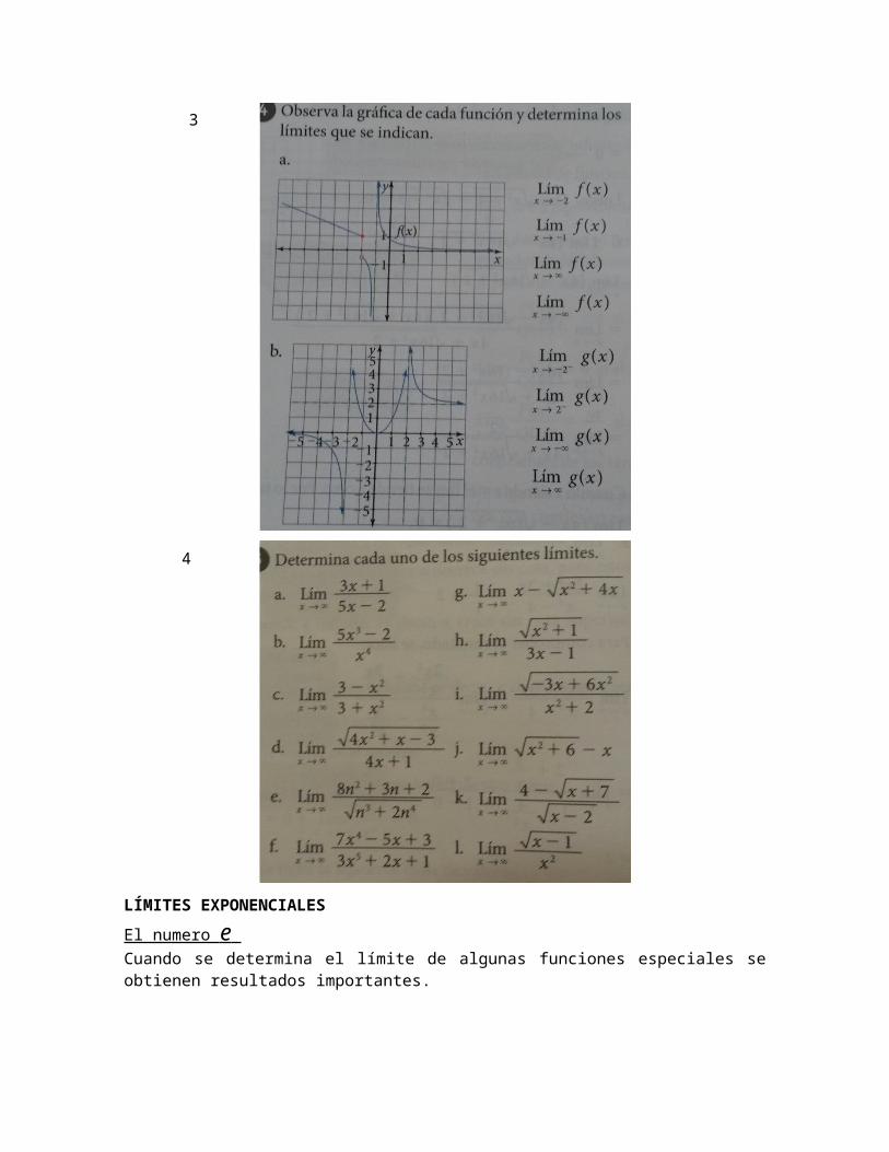
EJERCICIOS

1

2

LÍMITES EXPONENCIALES

El numero e Cuando se determina el límite de algunas funciones especiales se obtienen resultados importantes.

Si f ( x )=(1+ 1x )

x

para x∈Ζ+

, entonces, Límx→∞ (1+ 1x )

x

=e.

3

4

La tabla de valores y la gráfica de la función f ( x )=(1+ 1x )

x

, para x∈Ζ+

, se presenta a continuación.

x 1 2 3 4 5 6 7f(x) 2 2,25 2,370

32,4414

2,4883

2,5216

2,5465

Por lo tanto cuando x tiende a ∞ , entonces, f ( x )=(1+ 1x )

x

tiende a e≈2,71 .Los límites exponenciales más importantes son:

Límx→0

(1+x )1/ x=e Límx→∞

ex=∞ Límx→−∞

ex=0

Límites de la forma Límx→a

[ f ( x ) ]g( x ) o Límx→a

[ f ( x ) ]g( x )

Se presentan dos casos:Límites finitos:

Si Límx→a

f ( x )=Ly Límx→a

g ( x )=N, entonces,

Límx→a

[ f ( x ) ]g( x )=LNLímites infinitos:

Si Límx→∞

f ( x )=Ly Límx→a

g ( x )=+∞, entonces,

Límx→∞

[ f ( x ) ]g( x ) se calcula de acuerdo con los

siguientes resultados.

Lo=1 ;0∞=0 .

0L=¿ {0 , siL>0¿ ¿¿¿

∞L=¿ {∞ , siL>0 ¿ ¿¿¿

∞=∞;∞−∞=0 .

L∞=¿ {0 , si0<L<1¿ ¿¿¿

Asíntotas Horizontales:

La función f(x) tiene por asíntota horizontal la recta de ecuación y=b si, Límx→∞

f ( x )=b o Límx→∞

f ( x )=b .

Asíntotas Verticales:La función f(x) tiene por asíntota vertical la recta de ecuación x=a, si Límx→a−

f ( x )=±∞o Límx→a+

f ( x )=±∞

Asíntotas oblicuas:

Una función f(x) tiene asíntota oblicua si Límx→∞

f ( x )x o

Límx→−∞

f ( x )x

existe y es diferente de 0. La recta y=mx+bes la ecuación de la asíntota oblicua de f(x) si:

Límx→∞

[ f ( x )−(mx+b )]=0en donde:

m=Límx→∞

f ( x )x

m= Límx→−∞

f ( x )x

b=Límx→∞

[ f ( x )−mx ]

b= Límx→−∞

[ f ( x )−mx ]

EJERCICIOS

1. Encuentra el valor de cada límite.

a.

Límx→∞ ( 2 x3−3 x2−22+x2 )

2 x−1

e. Límx→0 ( tan xcos x )

3 x−1

b. Límx→0 ( 1−cos xx )

x−2

f.

Límx→1 ( 2

x+1 )cosπ2x

c.

Límx→1 (1+ 1

x−4 )x2−1

g. Límx→0 ( sen 5x2x )

x−1

d. Límx→0 ( sen5xsen 8 x )

2 x−2

h. Límx→1

(3x+2 )sen

π2x

2. Utiliza los límites para encontrar las asíntotas horizontales y verticales de cada función.

a. f ( x )= x

x+3 b. f ( x )= 2

x2−1

c. g( x )=3 x−1

x2−3 d. g( x )= x+1

x2−4

e. h( x )=√ x

x−3 f. f ( x )= x

x−1

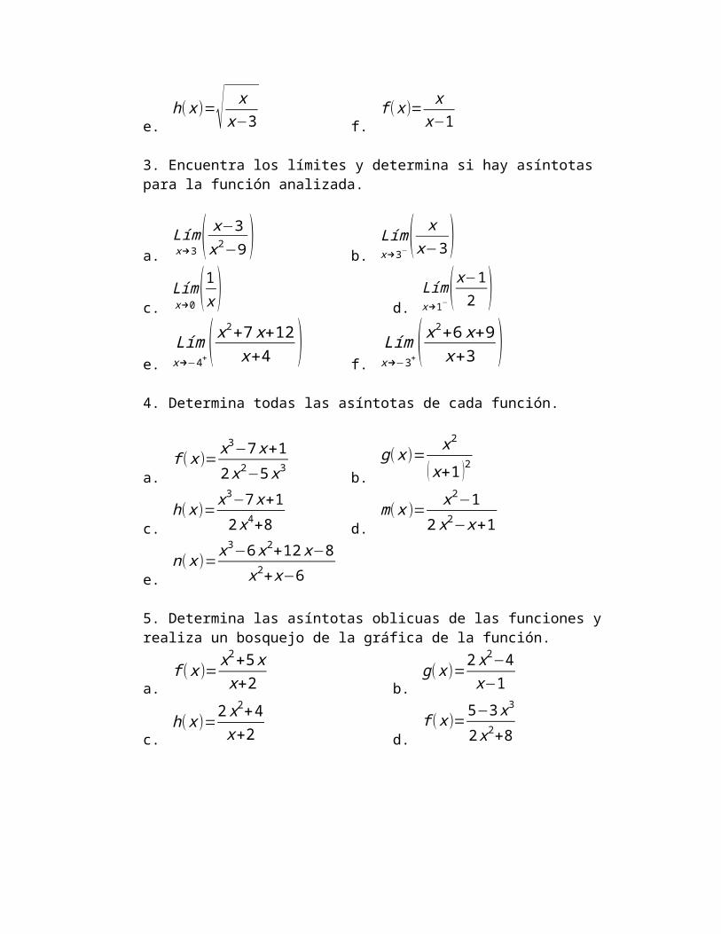
3. Encuentra los límites y determina si hay asíntotas para la función analizada.

a. Límx→3 ( x−3x2−9 ) b.

Límx→3−

( xx−3 )

c. Límx→0 ( 1x ) d.

Límx→1−

( x−12 )

e. Límx→−4+( x

2+7 x+12x+4 )

f. Límx→−3+

( x2+6 x+9x+3 )4. Determina todas las asíntotas de cada función.

a. f ( x )= x

3−7 x+12x2−5 x3 b.

g( x )= x2

( x+1 )2

c. h( x )= x

3−7 x+12 x4+8 d.

m( x )= x2−12 x2−x+1

e. n( x )= x

3−6 x2+12 x−8x2+x−6

5. Determina las asíntotas oblicuas de las funciones y realiza un bosquejo de la gráfica de la función.

a. f ( x )= x

2+5 xx+2 b.

g( x )=2 x2−4x−1

c. h( x )=2 x

2+4x+2 d.

f ( x )=5−3 x3

2 x2+8