Publication quality tables in Stata: a tutorial for the tabout program Ian Watson [email protected] Introduction tabout is a Stata program for producing publication quality tables.Ƭ It is more than just a means of exporting Stata results into spreadsheets, word processors, web browsers or compilers like L A T E X. tabout is actually a complete table building program. is tutorial is intended to present a complete overview of tabout, with numerous examples of syntax and the kind of tables produced. You might like to ick ahead and skim these examples before reading the more detailed exposition which follows. is tutorial has been around for a number of years but the current version makes use of colour and shading (to make it more readable) and also presents the tabout code in large blocks. Previously some of the preparatory Stata code, such as recoding variables, was only shown at the beginning of a set of tables. is meant that a user who just wanted to try out one particular table might have found that their results did not match the examples in this tutorial. At the risk of tedious repetition for those dedicated enough to begin at the beginning, the tutorial is now organised so that each example of code is ‘self contained’. e reader can now run any one of the examples in isolation and be guaranteed that the results should match what they see in this tutorial. All of the examples have sub-headings, so that readers can see at a glance what the particular example is illustrating. Finally, all of the examples are available in Stata do les which are installed when tabout is installed from the SSC archives. e le examples_tab.do contains all the code for tab-delimited output (the default) and the le examples_tex.do contains the code for L A T E X output. I say a user’s results should match the examples in this tutorial, but I should add a caveat. I oen get emails from tabout users who don’t get exactly the same presentation quality which they see in this tutorial. is is due to the fact that this tutorial uses L A T E X and makes use of the L A T E X facilities built in to tabout to optimise L A T E X code. ese users are oen exporting their results to MS Excel or MS Word and do not appreciate that L A T E Xis a totally distinct universe and requires learning a ‘new system’ for managing Stata output. I discuss L A T E X more fully in the following pages, but would stress here that tabout has many advantages for Stata users who are content to work in Excel or Word. In particular, it can automate many of the more tedious aspects of table production. Having dispensed with the housekeeping, it’s now time to explain what tabout actually does. In essence, tabout allows a novice Stata user to produce multiple panels of cross-tabulations, and to lay out the data in a number of different ways. e output can be oneway or twoway tables of frequencies and/or percentages, as well as summary statistics (means medians etc). Standard errors and/or condence intervals, based on Stata’s svy commands, can also be included. Furthermore, Ƭ Current version 2.0.6. 26 November 2012; Tutorial version 26 January 2013 Tutorial for tabout version 2.0.6 – 26 January 2013 1

Tabout Tutorial
Jan 02, 2016
stata tutorial for tab out
Welcome message from author
This document is posted to help you gain knowledge. Please leave a comment to let me know what you think about it! Share it to your friends and learn new things together.
Transcript
Publication quality tables in Stata:a tutorial for the tabout program
Introductiontabout is a Stata program for producing publication quality tables. It is more than just a means ofexporting Stata results into spreadsheets, word processors, web browsers or compilers like LATEX.tabout is actually a complete table building program. is tutorial is intended to present a completeoverview of tabout, with numerous examples of syntax and the kind of tables produced. Youmightlike to ick ahead and skim these examples before reading the more detailed exposition whichfollows.
is tutorial has been around for a number of years but the current versionmakes use of colourand shading (tomake itmore readable) and also presents the tabout code in large blocks. Previouslysome of the preparatory Stata code, such as recoding variables, was only shown at the beginning ofa set of tables. is meant that a user who just wanted to try out one particular table might havefound that their results did not match the examples in this tutorial. At the risk of tedious repetitionfor those dedicated enough to begin at the beginning, the tutorial is now organised so that eachexample of code is ‘self contained’. e reader can now run any one of the examples in isolationand be guaranteed that the results should match what they see in this tutorial. All of the exampleshave sub-headings, so that readers can see at a glance what the particular example is illustrating.Finally, all of the examples are available in Stata do les which are installed when tabout is installedfrom the SSC archives. e le examples_tab.do contains all the code for tab-delimited output (thedefault) and the le examples_tex.do contains the code for LATEX output.
I say a user’s results should match the examples in this tutorial, but I should add a caveat. Ioen get emails from tabout users who don’t get exactly the same presentation quality which theysee in this tutorial. is is due to the fact that this tutorial uses LATEX and makes use of the LATEXfacilities built in to tabout to optimise LATEX code. ese users are oen exporting their resultsto MS Excel or MS Word and do not appreciate that LATEXis a totally distinct universe and requireslearning a ‘new system’ formanaging Stata output. I discuss LATEXmore fully in the following pages,but would stress here that tabout has many advantages for Stata users who are content to work inExcel or Word. In particular, it can automate many of the more tedious aspects of table production.
Having dispensed with the housekeeping, it’s now time to explain what tabout actually does.In essence, tabout allows a novice Stata user to produce multiple panels of cross-tabulations, andto lay out the data in a number of different ways. e output can be oneway or twoway tables offrequencies and/or percentages, as well as summary statistics (meansmedians etc). Standard errorsand/or con dence intervals, based on Stata’s svy commands, can also be included. Furthermore,
Current version 2.0.6. 26 November 2012; Tutorial version 26 January 2013
Tutorial for tabout version 2.0.6 – 26 January 2013 1
a number of statistics (chi2, Gamma, Cramer’s V, Kendall’s tau) can be placed at the bottom ofeach panel. Finally, formatting of cell contents is simple, and allows users to choose the numberof decimal places, and to insert percentage symbols and currency symbols. Before looking moreclosely at some of the features available in tabout, it is worth outlining brie y the design principlesbehind the program.
At a minimum, publication quality tables should be both informative and aesthetically pleas-ing. In his discussion of what makes for graphical excellence, Edward Tue (2001) listed severalimportant aspects of data presentation including the following:
1. present many numbers in a small space;2. encourage the eye to compare different pieces of data.
While Tue had graphs in mind, the same advice helps de ne what is meant by ‘informative’when it comes to tables. In the case of tabout, multiple panels play this role. As will become evidentlater, repeating vertical panels allow for the succinct presentation of a considerable amount of data.Moreover, comparisons between populations and sub-populations within the one table are alsoeasily achieved using tabout.
Tue’s book also canvassed aesthetics, though some critics might argue that his minimalistapproach to many of the classic statistical graphs has gone too far. Nevertheless, his core idea ofmaximising the data component, andminimising the decorative junk, makes for a lot of sense whenit comes to table design. It coincides with the sentiments of Simon Fear, the author of the LATEXpackage, booktabs (2003).With respect to the use of lines (called rules in LATEX), Fear advocated thatone should ‘never, ever use vertical rules’, and, more controversially, one should ‘never use doublerules’. ese principles—or at least the rst one—are commonly followed in the tables presented inacademic journals, and routinely violated in the business-type tables produced by spreadsheets.
Further re nements suggested by Fear (and implemented in his booktabs package) include:increasing the thickness of rules at the top and bottom of tables compared with the lines used forthe mid-rules; and using a small but discernible amount of additional spacing above and belowrules. Anyone who has tried to implement these principles inside a word processor knows howtedious this task is, making LATEX the obvious choice for achieving aesthetic goals such as these.In the case of tabout, the aesthetics largely come through exporting the output as a LATEX docu-ment and making use of a number of tabout options. ese include variable rule thicknesses andspacings, rules which span a set number of columns, and the rotation of value labels in the tableheaders to achieve an economical layout which avoids the ugliness of hyphenation. An additionaladvantage in using LATEX with tabout is the ease with which it allows for the batch production oftables, particularly large numbers of routine tables (as oen occurs in an appendix).
For Stata users contemplating leaving their word processors behind and trying out LATEX, thereare a large number of tutorials and other freematerials available on the web. Two books which havebeen a staple in my library for many years are Goossens et al. (1994) and Kopka and Daly (1999),both of which have been recently updated.
Despite my bias towards LATEX, tabout also provides many advantages to those Stata users whoimport their descriptive tables into spreadsheets or word processors, or require html output. Aswill be evident below, these users can also gain great efficiencies in using tabout, since very littlefurther processing of the cell entries is required once the appropriate options have been turned onin tabout.
Principles of user-friendliness underlie both the design and the syntax of tabout. While taboutaims to offer considerable customisation and exibility to the end user, it tries to do this withoutbecoming overly complex. It stays close to Stata principles, and also implements a number of con-sistent requirements in its syntax. ere is a preference for single terms as options, either as a switch
2 Tutorial for tabout version 2.0.6 – 26 January 2013
(simply turning on svy, for example to achieve survey results) or as a switchwith a single value (suchas the layout option). tabout avoids options within options, with the consequent need for numer-ous balanced parentheses. Instead, using two or three separate switches (where needed), each witha single value, is the preferred approach. e n option, for example, which provides sample countsin a table has ve siblings: an npos (the position), an nlab (the label), an nwt (the weight), an nnoc
to suppress the display of commas and an noffset to control placement of n counts. tabout alsoallows for the ‘incomplete’ entry of values, and makes up the additional values by repeating thelast value entered (for example, with formats or labels). Finally, tabout also tries to capture mostsyntax errors at the outset and to provide a simple explanation. To facilitate this, a table outliningthe allowable features of tabout is presented to users when they make syntax errors. (is table ispresented later in this tutorial.)
OverviewWhat kinds of tables does tabout produce? Using a simple terminology, you can produce basictables and summary tables. e rst are twoway and oneway tables of frequencies and percentages.Essentially, all of the output from Stata’s tabulate is available in a basic table. You can also producebasic tables with standard errors and con dence intervals, re ectingmost of the output from Stata’ssvy:tab commands. As for summary tables, these are twoway or oneway tables of summary stat-istics derived from Stata’s summarize command but laid out in a much more aesthetically pleasingfashion. In many respects, these tables mimic most of the output from Stata’s tabstat and table
commands. Finally, you can also have summary tables with standard errors and con dence inter-vals, though this is restricted tomean values. ese tables make use of Stata’s svy:mean command.With a large dataset, the survey option in tabout can be quite slow. is is partly because the sur-vey commands run slower in Stata 9 than they did in previous releases, and partly because taboutneeds to run the survey commands twice to retrieve column and row totals. e latest version oftabout now includes the ‘dot counter’ view, which indicates to the user that something is actuallyhappening (however, slowly).
With a basic table, the cells in a table can be any one or all of the following: frequencies, cellpercentages, column percentages, row percentages, cumulative percentages. With summary tablesthe list is quite extensive: N mean var sd skewness kurtosis sum uwsum min max count median iqrr9010 r9050 r7525 r1050 p1 p5 p10 p25 p50 p75 p90 p95 p99.
ere is considerable exibility in the layout of the tables. All tables can be produced usingmul-tiple ‘vertical’ panels if desired. A command like tabout occupation industry south will pro-duce two vertical panels (variables occupation and industry) cross-tabulated against a ‘horizontal’variable, south. e cell contents can be laid out in columns or rows (for example, frequencies andcolumn percentages alternating, as in: No. % No. % No. %). ey can also be laid out incolumn block (abbreviated to cb) or row block (abbreviated to rb) mode. For example, frequenciesand column percentages can be in contiguous blocks, as in: No. No. No. % % %).
As well as the contents of the cells, additional information can be placed in the table. e mostnotable of these inclusions are sample counts (or population estimates),⁴ which can be placed inthe far right column, along the bottom of the table or alongside the value labels in the rst column.A range of statistics can also be included at the bottom of the table. ese consist of: Pearson
If an if or in condition is speci ed with any of the svy options, tabout makes use of the subpopulation option, asrecommended in the Stata manual.e uwsum is notmainstream Stata. It stands for ‘unweighted sum’ and is a useful statistic in tables where you to presentweighted data, but would like one (or more) columns to contain an unweighted sum of a variable. For example, ‘uwsumsubpop’ can be used to create an ‘n’ count in the middle of a table of means.
⁴ e main difference between these two is that the latter are weighted counts, achieved through tabout’s nwt option.Note that you need to use the pop option when you are also using survey data (with the svy option) in order to achieveweighted population estimates rather than sample counts. is is a new feature / bug x added to taboutVersion 2.0.4.
Tutorial for tabout version 2.0.6 – 26 January 2013 3
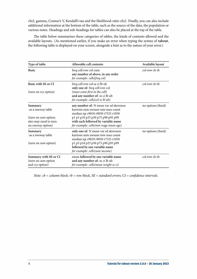
chi2, gamma, Cramer’s V, Kendall’s tau and the likelihood-ratio chi2. Finally, you can also includeadditional information at the bottom of the table, such as the source of the data, the population orvarious notes. Headings and sub-headings for tables can also be placed at the top of the table.
e table below summarises these categories of tables, the kinds of contents allowed and theavailable layouts. (As mentioned earlier, if you make an error when typing the syntax of tabout,the following table is displayed on your screen, alongside a hint as to the nature of your error.)
Type of table Allowable cell contents Available layout
Basic freq cell row col cum col row cb rbany number of above, in any orderfor example: cells(freq col)
Basic with SE or CI freq cell row col se ci lb ub col row cb rbonly one of: freq cell row col
(turn on svy option) (must come rst in the cell)and any number of: se ci lb ubfor example: cells(col se lb ub)
Summary any number of: N mean var sd skewness no options ( xed)-as a oneway table kurtosis sum uwsum min max count
median iqr r9010 r9050 r7525 r1050(turn on sum option; p1 p5 p10 p25 p50 p75 p90 p95 p99also may need to turn with each followed by variable nameon oneway option) for example: cells(min wage mean age)
Summary only one of: N mean var sd skewness no options ( xed)-as a twoway table kurtosis sum uwsum min max count
median iqr r9010 r9050 r7525 r1050(turn on sum option) p1 p5 p10 p25 p50 p75 p90 p95 p99
followed by one variable namefor example: cells(sum income)
Summary with SE or CI mean followed by one variable name col row cb rb(turn on sum option and any number of: se ci lb uband svy option) for example: cells(mean weight se ci)
Note: cb = column block; rb = row block, SE = standard errors; CI = con dence intervals.
4 Tutorial for tabout version 2.0.6 – 26 January 2013
Syntax
tabout varlist[weight
][if
][in
]using
[, replace append cells(contents) format(string)
clab(string) layout(layouts) oneway sum stats(statstypes)
VARIOUS ‘N’ OPTIONS:
npos(positions) nlab(string) nwt(string) nnoc noffset(textrm string)
VARIOUS SVY OPTIONS:
svy sebnone cibnone cisep(string) ci2col percent level(#) pop
USER CUSTOMISATION OF LABELS:
total(string) ptotal(totaltype) h1(string) h2(string) h3(string)
STYLE OPTIONS, MOSTLY FOR LATEX OUTPUT:
style(styles) lines(linetypes) font(fontstyles) bt rotate(#) cl1(#-#) cl2(#-#) cltr1(string)
cltr2(string)
OPTIONS RELATED TO EXTERNAL FILES:
body topf(string) botf(string) topstr(string) botstr(string) psymbol(string) delim(string)
MISCELLANEOUS OPTIONS: dpcomma money(string) mi sort chkwtnone debug noborder
show(showtypes) wide(#)]
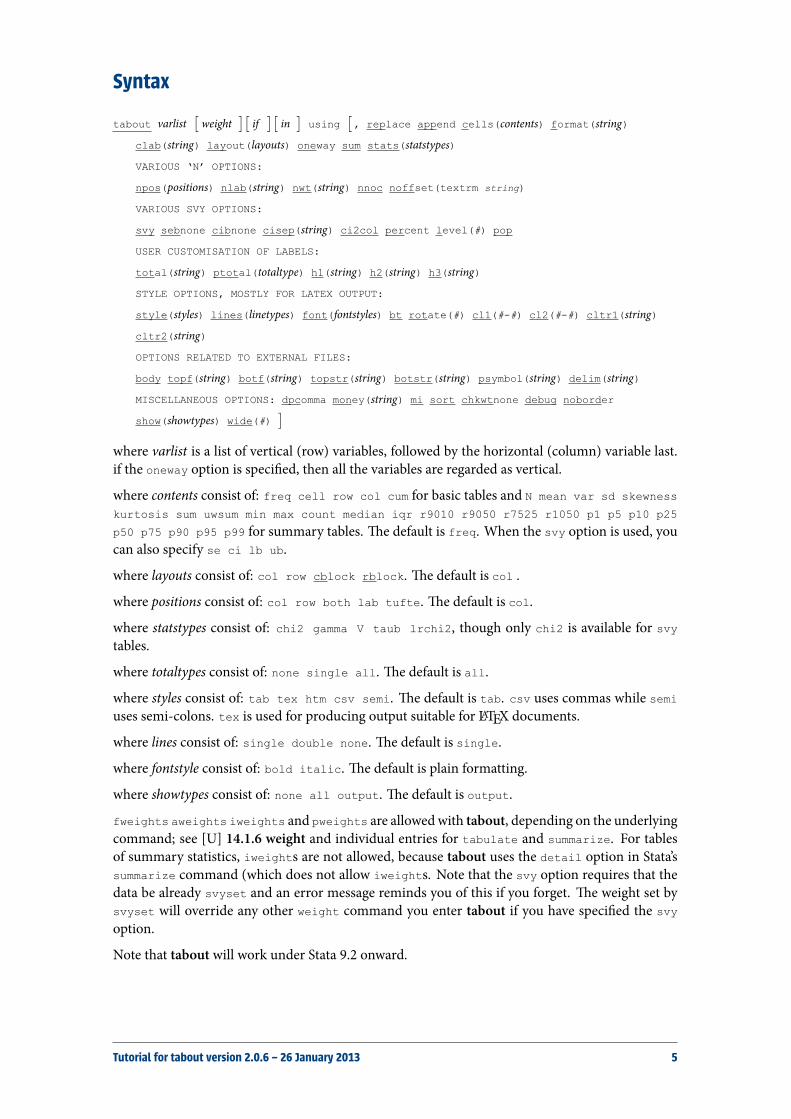
where varlist is a list of vertical (row) variables, followed by the horizontal (column) variable last.if the oneway option is speci ed, then all the variables are regarded as vertical.
where contents consist of: freq cell row col cum for basic tables and N mean var sd skewness
kurtosis sum uwsum min max count median iqr r9010 r9050 r7525 r1050 p1 p5 p10 p25
p50 p75 p90 p95 p99 for summary tables. e default is freq. When the svy option is used, youcan also specify se ci lb ub.
where layouts consist of: col row cblock rblock. e default is col .
where positions consist of: col row both lab tufte. e default is col.
where statstypes consist of: chi2 gamma V taub lrchi2, though only chi2 is available for svytables.
where totaltypes consist of: none single all. e default is all.
where styles consist of: tab tex htm csv semi. e default is tab. csv uses commas while semiuses semi-colons. tex is used for producing output suitable for LATEX documents.
where lines consist of: single double none. e default is single.
where fontstyle consist of: bold italic. e default is plain formatting.
where showtypes consist of: none all output. e default is output.
fweights aweights iweights and pweights are allowedwith tabout, depending on the underlyingcommand; see [U] 14.1.6 weight and individual entries for tabulate and summarize. For tablesof summary statistics, iweights are not allowed, because tabout uses the detail option in Stata’ssummarize command (which does not allow iweights. Note that the svy option requires that thedata be already svyset and an error message reminds you of this if you forget. e weight set bysvyset will override any other weight command you enter tabout if you have speci ed the svy
option.
Note that tabout will work under Stata 9.2 onward.
Tutorial for tabout version 2.0.6 – 26 January 2013 5

Optionsusing is required, and indicates the lename for the output. Some applications (particularly MS
Excel) ‘lock’ les when they’re open. tabout cannot write to these les and consequentlyissues an error message, suggesting that you check to see if the le is already open inanother application. ere is now a discussion of this problem in the ‘Tips and Tricks’section below.
replace and append are le options, and determine whether the current output will overwrite anexisting le, or be appended to the end of that le. If you omit append or replace, taboutissues a warning if the le already exists.
cells determines the contents of table cells. As the table on the previous page showed, youcan enter any one or more of freq cell row col cum in a basic table. ey can be inany order. When you choose the svy option, you can only have one of these choices, andit must come rst. e additional choices which are then available are: se ci lb ub.For summary tables, you can have any of the contents listed earlier. If you are creatinga twoway table, only one summary statistic may go in a cell (eg. median wage); if it’s aoneway table, any number of statistics (followed by a variable name) may go in the cell(eg. median wage mean age iqr weight). When you choose the svy option withsummary tables, only mean is allowed (eg. mean wage se ci.)
format indicates the number of decimal points. Unlike mainstream Stata, this option onlyrequires a number. Donot enter ‘%’ or ‘f ’ symbols. You can however, enter c for comma, pfor percentage, and m for money (currency) and you can use the money option (see below)to specify the currency. For example, you might enter f(0c 1p 1p 2) to produce: 1,2919.2% 10.3% 23.93. e entries should be in the same order as the cells order, that is, iffreq comes rst, then 0c should come rst if you want 0 decimal points (with commas)as the format for frequencies. You do not have to type in the same number of formatentries as there are cell entries. If you include more, tabout ignores them; if you includeless, the last format entry is repeated for the remaining cell entries. You can change thedecimal point and thousand separators to the style favoured in some European countries(, for decimal points . for thousands) using the dpcomma option (see below).
clab determines the column headings for the third row of the table, that is, the headings justabove the data. By default, tabout places the ‘horizontal’ variable’s name in the rst row,its value labels in the second row, and an abbreviation for the cell contents (eg. No. Row% etc) in the third row. You can over-ride all of these defaults using the h1 h2 and h3
options (see below). Most of the time, however, it will only be the third row which youneed to change, so the clab option makes this easy for you. Just enter the column titlesas you want them to display, without quote marks or other symbols. However, you mustinclude underscores between words if there are spaces in the column title, for exampleclab(No. Row_% Col_%). You do not have to type in the same number of clab entriesas there are cell entries. If you include more, tabout ignores them; if you include less, thelast clab entry is repeated for the remaining cell entries. For example if your cell entrywas freq col row cum you could just enter clab(No. %)and all but the rst column ofdata would have % symbols at the top.
layout determines how the columns will be laid out. ey can be in alternating columns (No.% No. % No. %) and alternating rows (No. on the rst row, % on the next two,then back to No. and so on). ey can be in column blocks, or in row blocks, where thedata is kept contiguous, for example: No. No. No. % % %. e exception tothis is summary tables where the layout is xed and you have no choice. (However, an
6 Tutorial for tabout version 2.0.6 – 26 January 2013
exception to this is the svy option, which can be laid out using all of these options. Seethe earlier table for clari cation.)
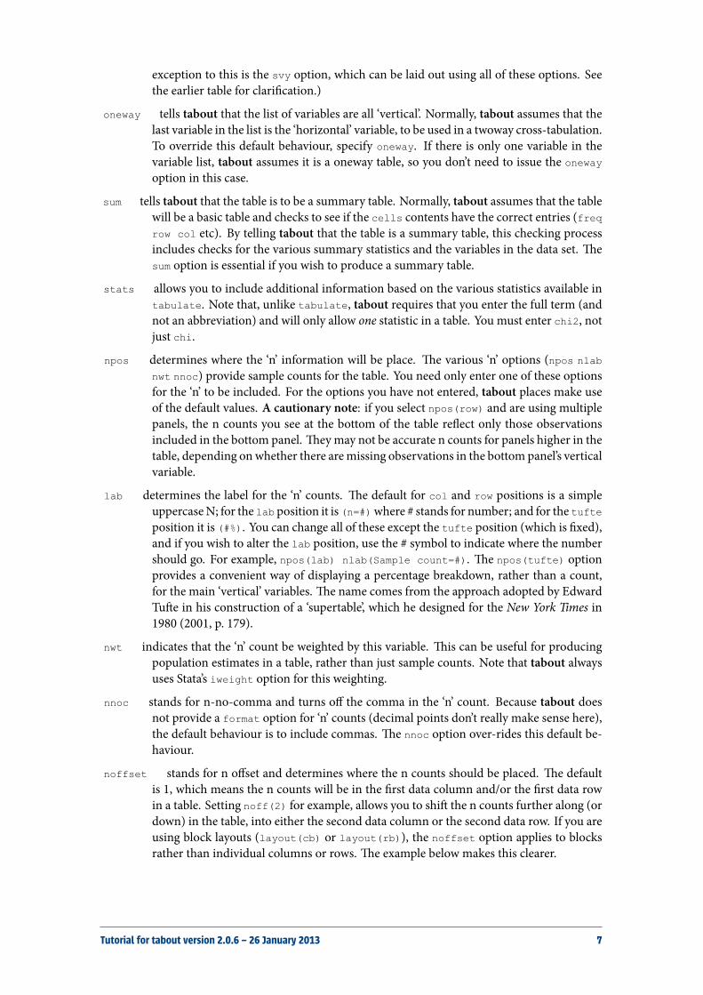
oneway tells tabout that the list of variables are all ‘vertical’. Normally, tabout assumes that thelast variable in the list is the ‘horizontal’ variable, to be used in a twoway cross-tabulation.To override this default behaviour, specify oneway. If there is only one variable in thevariable list, tabout assumes it is a oneway table, so you don’t need to issue the oneway
option in this case.
sum tells tabout that the table is to be a summary table. Normally, tabout assumes that the tablewill be a basic table and checks to see if the cells contents have the correct entries (freqrow col etc). By telling tabout that the table is a summary table, this checking processincludes checks for the various summary statistics and the variables in the data set. esum option is essential if you wish to produce a summary table.
stats allows you to include additional information based on the various statistics available intabulate. Note that, unlike tabulate, tabout requires that you enter the full term (andnot an abbreviation) and will only allow one statistic in a table. You must enter chi2, notjust chi.
npos determines where the ‘n’ information will be place. e various ‘n’ options (npos nlab
nwt nnoc) provide sample counts for the table. You need only enter one of these optionsfor the ‘n’ to be included. For the options you have not entered, tabout places make useof the default values. A cautionary note: if you select npos(row) and are using multiplepanels, the n counts you see at the bottom of the table re ect only those observationsincluded in the bottom panel. ey may not be accurate n counts for panels higher in thetable, depending onwhether there aremissing observations in the bottom panel’s verticalvariable.
lab determines the label for the ‘n’ counts. e default for col and row positions is a simpleuppercaseN; for the lab position it is (n=#)where # stands for number; and for the tufteposition it is (#%). You can change all of these except the tufte position (which is xed),and if you wish to alter the lab position, use the # symbol to indicate where the numbershould go. For example, npos(lab) nlab(Sample count=#). e npos(tufte) optionprovides a convenient way of displaying a percentage breakdown, rather than a count,for the main ‘vertical’ variables. e name comes from the approach adopted by EdwardTue in his construction of a ‘supertable’, which he designed for the New York Times in1980 (2001, p. 179).
nwt indicates that the ‘n’ count be weighted by this variable. is can be useful for producingpopulation estimates in a table, rather than just sample counts. Note that tabout alwaysuses Stata’s iweight option for this weighting.
nnoc stands for n-no-comma and turns off the comma in the ‘n’ count. Because tabout doesnot provide a format option for ‘n’ counts (decimal points don’t really make sense here),the default behaviour is to include commas. e nnoc option over-rides this default be-haviour.
noffset stands for n offset and determines where the n counts should be placed. e defaultis 1, which means the n counts will be in the rst data column and/or the rst data rowin a table. Setting noff(2) for example, allows you to shi the n counts further along (ordown) in the table, into either the second data column or the second data row. If you areusing block layouts (layout(cb) or layout(rb)), the noffset option applies to blocksrather than individual columns or rows. e example below makes this clearer.
Tutorial for tabout version 2.0.6 – 26 January 2013 7
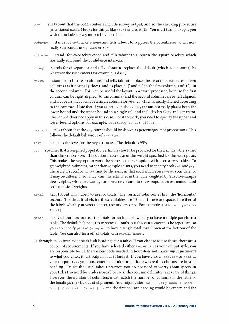
svy tells tabout that the cell contents include survey output, and so the checking procedure(mentioned earlier) looks for things like se, ci and so forth. You must turn on svy is youwish to include survey output in your table.
sebnone stands for se-brackets-none and tells tabout to suppress the parentheses which nor-mally surround the standard errors.
cibnone stands for ci-brackets-none and tells tabout to suppress the square brackets whichnormally surround the con dence intervals.
cisep stands for ci-separator and tells tabout to replace the default (which is a comma) bywhatever the user enters (for example, a dash).
ci2col stands for ci-in-two-columns and tells tabout to place the lb and ub estimates in twocolumns (as it normally does), and to place a ‘[’ and a ‘,’ in the rst column, and a ‘]’ inthe second column. is can be useful for layout in a word processor, because the rstcolumn can be right aligned (to the comma) and the second column can be le aligned,and it appears that you have a single column for your ci, which is neatly aligned accordingto the commas. Note that if you select ci in the cells, tabout normally places both thelower bound and the upper bound in a single cell and includes brackets and separator.e ci2col does not apply in this case. For it to work, you need to specify the upper andlower bound options, for example: cell(freq lb ub) ci2col.
percent tells tabout that the svy output should be shown as percentages, not proportions. isfollows the default behaviour of svy:tab.
level speci es the level for the svy estimates. e default is 95%.
pop speci es that aweighted population estimate should be provided for the n in the table, ratherthan the sample size. is option makes use of the weight speci ed by the nwt option.is makes the svy option work the same as the nwt option with non-survey tables. Toget weighted estimates, rather than sample counts, you need to specify both nwt and pop.e weight speci ed in nwtmay be the same as that used when you svyset your data, orit may be different. You may want the estimates in the table weighted by ‘effective samplesize’ weights, while you want your n row or column to show population estimates basedon ‘expansion’ weights.
total tells tabout what labels to use for totals. e ‘vertical’ total comes rst, the ‘horizontal’second. e default labels for these variables are ‘Total’. If there are spaces in either ofthe labels which you wish to enter, use underscores. For example, total(All_personsTotal).
ptotal tells tabout how to treat the totals for each panel, when you have multiple panels in atable. e default behaviour is to show all totals, but this can sometimes be repetitive, soyou can specify ptotal(single) to have a single total row shown at the bottom of thetable. You can also turn off all totals with ptotal(none).
h1 through to h3 over-ride the default headings for a table. If you choose to use these, there are acouple of requirements. If you have selected either tex or htm as your output style, youare responsible for all the various code needed. tabout does not make any adjustmentsto what you enter, it just outputs it as it nds it. If you have chosen tab, csv or semi asyour output style, you must enter a delimiter to indicate where the columns are in yourheading. Unlike the usual tabout practice, you do not need to worry about spaces inyour titles (no need for underscores!) because this column delimiter takes care of things.However, the number of delimiters must match the number of columns in the table orthe headings may be out of alignment. You might enter: h2( | Very good | Good |
Bad | Very bad | Total | N) and the rst column heading would be empty, and the
8 Tutorial for tabout version 2.0.6 – 26 January 2013
remaining columns would have the appropriate labels. Note that the npos(col) optionusually places the nlab on the h2 line so you may need to include this yourself in your h2label, as in the example just given. To suppress the display of any of these headings, enter‘nil’ into the appropriate option (for example, h3(nil)). While it is rare to write headingslonger than 256 characters, problems have been reported when this limit is exceeded.
style e default is style(tab), which is useful for importing into spreadsheets or word pro-cessors. Note that the rst row always has the correct number of tabs, even when a singletitle is involved. is helps other applications parse the table correctly. Note also that therepetition of labels in headings can be easily dealt with by using a ‘merge cells’ commandin your spreadsheet or word processor. e style(csv) and style(semi) options areuseful for importing into spreadsheets (like MS Excel) because the le generally opensimmediately as a spreadsheet. Note, however, that some spreadsheets ignore trailing 0s,so this may muck up your neat formatting. To avoid this, export the table from tabout asstyle(tab) and use the wizard in your spreadsheet to indicate that all columns are ‘text’rather than ‘general’.
lines indicates howmuch space (for style(tab), style(csv) and style(semi)) or howmanylines (for style(tex)) should separate tables between panels. e default is single.
font only applies to style(tex) and style(htm) and provides bold and italic fonts for the‘vertical’ variable names and the ‘horizontal’ variable names and value labels. e totalsare also given this font. You can also use the h1 to h3 options to manually set up fonts foryour titles.
bt only applies to users of LATEX, and requires that you have the booktabs package installed.is allows the use of the toprule, midrule and bottomrule commands, rather than theusual hline command. It produces more pleasing output.
rotate only applies to users of LATEX, and can be used to rotate the ‘horizontal’ variable’s labelsthrough whatever angle is entered in this option. For example, rotate(60) producesquite a pleasing effect. You will also need to include the following LATEX code (courtesyof Goossens et al. (1997, pp. 48–49)) in your document’s preamble:
LaTeX code for rotation of table headings
\newcommand{\rot}[2]{\rule{1em}{0pt}%
\makebox[0cm][c]{\rotatebox{#1}{\ #2}}}
cl1 and cl2 only apply to users of LATEX, and also requires that you use the booktabs package inyour LATEX document. ese options can be used to place horizontal lines which spanseveral columns (called, column lines, hence cl) and which are placed between the rstand second heading rows, and between the second and third heading rows (hence twosets). You enter the column numbers which you wish to span, separated with a dash. Forexample, to place a line under the ‘horizontal’ variable’s name, youmight enter: cl1(2-6)in a table with six columns. If you are entering lines spanning blocks of columns (2-4 5-7), youmight need to ne tune the gap between them using cltr1 and cltr2. By default,whenever you specify either of the cl options, taboutplaces a small gap (0.75em) betweenadjacent lines.
cltr1 and cltr2 stand for column-line-trim, and allow you to specify an amount of trim to beapplied to the le side of the cl1 or cl2 lines which you have entered. You can specifythe amount in whatever acceptable texmeasurement you like. For example: cl2(2-3 4-5
6-7) cltr2(1.5em). As just noted, the default amount is 0.75em.
body is used to insert some basic html or LATEX code above and below the table. is allows youto view the table without further coding.
Tutorial for tabout version 2.0.6 – 26 January 2013 9

topf and botf allow you to insert code stored in les which tabout can insert above and below thetables. ese are particularly useful for html and LATEX users, and allow you to controlthe layout of the tables more precisely. All users will nd them useful as a way of insert-ing additional information above and below the table, such as notes, populations, datasources (for the bottom of the table) and titles (for the top of the table).
topstr and botstr contain text which you can pass to the topf and botf les. is text willbe inserted into the les where ever the placeholder (default #) has been placed. Notethat each placeholder must be on a separate line in these les. e strings designated inthe topstr and botstr must be separated with the pipe delimiter (or other user-chosendelimiter) if there is more than one block of text being passed.
psymbol stands for placeholder-symbol and can be any symbol the user chooses. e defaultis # and it provides a ‘placeholder’ in the stored les (the topf and botf) which taboutplaces above and below the tables.
delimit can be any symbol the user chooses. e default is the pipe delimiter as shown inthe earlier example. It is used to specify columns within the h1 to h3 options, and forseparating the contents of the topstr and botstr options.
dpcomma speci es that tabout should use commas for decimal points and periods (full-stops)for thousand separators. is style is common in many European countries. is op-tion affects the presentation of both the tabular output and the statistics when these arerequested (such as chi2).
money indicates the currency to be used if you have chosen the money format. For example,format(2m) money(£). You can enter any symbol that your keyboard allows. For LaTeXusers, you can enter any text which LaTeX accepts, though you may need to includequotes.
mi speci es that tabout should display missing values. is works the same as the mi option inStata’s tabulate command.
sort speci es that tabout should display values in oneway tables in descending order of fre-quency. is works the same as the sort option in Stata’s tabulate oneway command.Note that if you issue this for a twoway table, you will receive an error message. isis because tabout is built on top of tabulate and the latter does not support sorting intwoway tables.
chkwtnone prevents tabout from checking the legality of your weights. Stata commands willnot allow you to use non-integer frequency weights and tabout normally checks for this.You can over-ride this behaviour with the tt chkwtnone option. Note that this optiondoes not stop Stata itself from refusing to use non-integer frequency weights.
debug shows you most of the underlying Stata commands (though not for summary tables)from which the tables are built. is can be useful for con rming your results.
noborder only applies to html output, and determines whether the table and cells should besurrounded by borders. is only applies when the body option is turned on.
show determines what will be seen on the screen. e show(all) option displays the nal tableoutput as well as the Mata string matrices which are used to build this nal output. econtents of these matrices may not exactly match the nal output, in terms of formattingand labelling. e show(none) option suppresses all output except for the name of thele to which the table has been exported. e default option is to show the output which
has been sent to a le. It may look messy on the screen, but open it in the appropriateapplication to check it rst before panicking.
10 Tutorial for tabout version 2.0.6 – 26 January 2013
wide is used in conjunction with show(all) and speci es the width of the columns in theMata matrices. e default is 10 spaces. Note that even if you reduce this to a very smallnumber, taboutwill always increase thewidth of the columns to accommodate thewidestcell entry in the data.
Some examplesIf you want to dive straight into the examples, please read this paragraph rst! e code whichaccompanies all the examples below has a line rep /// somewhere in the middle. If you are auser who only wants delimited text les—that is, you’re not a LATEX user—don’t use the code belowthis line. e code from style(tex) onward is for LATEX users. If you’re uncertain, just look at theancillary les for tabout: examples_tab.dowhich contains all the code for tab-delimited output (thedefault) and the le examples_tex.do which contains all the code for LATEX output.
In the following examples I present some tables based on several of Stata’s shipped datasets,though they mainly draw on the nlsw88.dta dataset. is is a handy dataset for illustration becauseit has so many categorical variables (apologies to those with a more medical inclination to theirstats.). All these shipped datasets can be loaded with the sysuse command. In the case of thenlsw88.dta, a weight variable was also constructed (using a random number multiplied tenfold) soas to demonstrate the svy option.
A note on the examples and typefaces. In the discussion up to now, and in the syntax andoptions sections above, this tutorial has followed the Stata convention and shown the commandoptions in the same way they are presented in the Stata manual.⁵ However, for clarity and readab-ility, from now on the typeface departs from the Stata convention in a couple of ways. Referencesto other Stata commands are in the normal roman font, but are bolded and references to tabout’sown options are in a sans serif blue font (Urbana SemiBold for those interested). is makes it easyto discern what the tabout options are, which should make it simpler when it comes to checkingthe options section when you want to read more about a particular feature.
A brief note on abbreviations is also worth making. In the examples which follow I use thefull wording in the rst part of the example code so that users will know what is going on. iseven applies to variable names, for example, using ‘occupation’ rather than the much shorter, ‘occ’.However, as the examples continue, I begin to use the abbreviations. If you’re not sure about this,check the syntax diagram where the underlining indicates the abbreviated version of an option.
While the actual tabout syntax (the code) in the following examples does follow the Stata con-vention of using a xed typewriter font, the background is shown as a grey shading. is makesit easier for the casual reader to see what is going on. In addition all of these blocks of syntax arelabelled so that they directly relate to the example output. e output itself is shown in a blue sansserif font. Cutting and pasting from these blocks of syntax into Stata should produce the same res-ults as you see in this tutorial. A word of warning though. If you cut and paste from a PDF le(like this tutorial) quotation marks may not copy correctly and you may come to grief with macros,since Stata requires you to distinguish between the back quote and the normal quote. is warningmainly applies to the Tips and Tricks section, where macros are used a fair bit.
For LATEX users, copying and pasting the code should produce identical results to those shownin this tutorial if you run the whole block. e only change you will need to make is to replacetable1.txt with table1.tex etc. e surrounding LATEX table commands are not shown, but are foundin the top le and bottom le text shown aer the examples section of this tutorial. Once you createthese les and place them in your ownworking directory, you should not need to worry about themagain.
⁵ e only exception to this has been that the word tabout has been presented in bold roman font throughout this tutorial,rather than the xed typewriter font normally used for Stata commands.
Tutorial for tabout version 2.0.6 – 26 January 2013 11
For thosewanting tab delimited output, stop at the line ‘replace’ and ignore the remaining LATEX-speci c code. In order to get the nice layouts and formats you see here, you’ll need to ddle withyour spreadsheet or word processing format controls. Finally, the replace option is redundant ifyou are only running these blocks of code once (so just ignore the error message).
If you prefer not to cut and paste from this tutorial, there are ancillary les which should installwhen you rst install tabout from the SSC archives. ese are example do- les which you candirectly run in Stata. ese les do not contain abbreviations and show the full name of all taboutoptions. ere are two les, which are just different versions of the same set of examples:
1. example_tex.do: which has all the code shown in these examples (that is, the additional LATEXoptions) and which sends the output to tex les; and
2. example_tab.do: which has the rst part of the code (up to the replace line), and which sendsoutput to tab-delimited text les.
ere are also two other ancillary lles—top.tex and bot.tex—which are used extensively in theLATEX examples. ere is a discussion of these les on page 33 below. You can either create yourown version of these les, or use the versions included here.
While it might appear from the following examples that the top le and bottom le options areonly useful for LATEX and html users, this is not the case. All of these examples show the source ofthe data as a note at the bottom of the table, and this device may be useful to all users. Indeed, en-capsulating titles, notes, sources, populations, weighting information, and so forth within the codewhich produces a table is a very good practice, and is particularly useful for the batch productionof tables, where copying such information bit-by-bit is error prone.
If you are a tab-delimited or csv user, have a look at the code for the contents of these les atthe end of this tutorial and you will see how you can also make use of top les and bottom les forincluding extra information with your tables. Just ignore the LATEX verbiage and focus on how the #symbol is used. is is the key to passing variable information, such as the population descriptionfor a table, to a xed set of phrases which are the same in all tables. For example, the phrases“Notes: Estimates weighted. Source: mysurvey.” might be repeated for all your table, while phraseslike “Population: All males over 21 year of ages” might vary between different tables. By using asimple bottom le (with the contents of the xed phrases) and then adding the # symbol at the end,you could then pass different ‘arguments’ (the phrases which vary) to the information which willprint at the bottom of your table.⁶
⁶ Note that while the examples in this tutorial just show the use of one argument being passed to a le, you can usemultiple arguments. Just add as many # symbols as you need. However, make sure each # symbol is on a new line inyour top and bottom les. Inside your tabout syntax, just use the pipe delimiter (or your de ned symbol) to separateall the arguments.
12 Tutorial for tabout version 2.0.6 – 26 January 2013
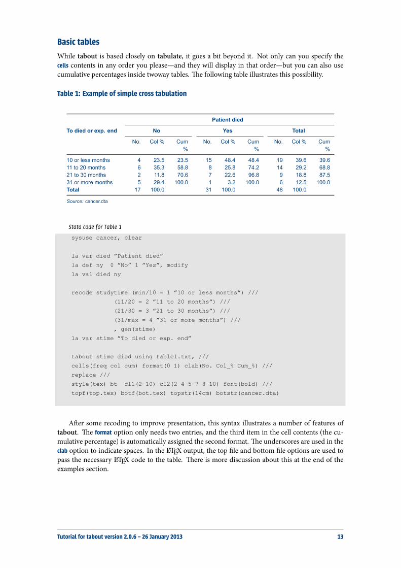
Basic tablesWhile tabout is based closely on tabulate, it goes a bit beyond it. Not only can you specify thecells contents in any order you please—and they will display in that order—but you can also usecumulative percentages inside twoway tables. e following table illustrates this possibility.
Table 1: Example of simple cross tabulation
Patient died
To died or exp. end No Yes Total
No. Col % Cum%
No. Col % Cum%
No. Col % Cum%
10 or less months 4 23.5 23.5 15 48.4 48.4 19 39.6 39.611 to 20 months 6 35.3 58.8 8 25.8 74.2 14 29.2 68.821 to 30 months 2 11.8 70.6 7 22.6 96.8 9 18.8 87.531 or more months 5 29.4 100.0 1 3.2 100.0 6 12.5 100.0Total 17 100.0 31 100.0 48 100.0
Source: cancer.dta
Stata code for Table 1
sysuse cancer, clear
la var died ”Patient died”
la def ny 0 ”No” 1 ”Yes”, modify
la val died ny
recode studytime (min/10 = 1 ”10 or less months”) ///
(11/20 = 2 ”11 to 20 months”) ///
(21/30 = 3 ”21 to 30 months”) ///
(31/max = 4 ”31 or more months”) ///
, gen(stime)
la var stime ”To died or exp. end”
tabout stime died using table1.txt, ///
cells(freq col cum) format(0 1) clab(No. Col_% Cum_%) ///
replace ///
style(tex) bt cl1(2-10) cl2(2-4 5-7 8-10) font(bold) ///
topf(top.tex) botf(bot.tex) topstr(14cm) botstr(cancer.dta)
Aer some recoding to improve presentation, this syntax illustrates a number of features oftabout. e format option only needs two entries, and the third item in the cell contents (the cu-mulative percentage) is automatically assigned the second format. e underscores are used in theclab option to indicate spaces. In the LATEX output, the top le and bottom le options are used topass the necessary LATEX code to the table. ere is more discussion about this at the end of theexamples section.
Tutorial for tabout version 2.0.6 – 26 January 2013 13
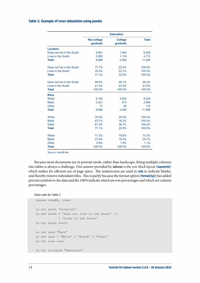
Table 2: Example of cross tabulation using panels
Education
Not collegegraduate
Collegegraduate
Total
LocationDoes not live in the South 5,091 1,464 6,555Lives in the South 3,595 1,118 4,713Total 8,686 2,582 11,268
Does not live in the South 77.7% 22.3% 100.0%Lives in the South 76.3% 23.7% 100.0%Total 77.1% 22.9% 100.0%
Does not live in the South 58.6% 56.7% 58.2%Lives in the South 41.4% 43.3% 41.8%Total 100.0% 100.0% 100.0%
RaceWhite 6,192 2,063 8,255Black 2,421 473 2,894Other 73 46 119Total 8,686 2,582 11,268
White 75.0% 25.0% 100.0%Black 83.7% 16.3% 100.0%Other 61.3% 38.7% 100.0%Total 77.1% 22.9% 100.0%
White 71.3% 79.9% 73.3%Black 27.9% 18.3% 25.7%Other 0.8% 1.8% 1.1%Total 100.0% 100.0% 100.0%
Source: nlsw88.dta
Because most documents are in portrait mode, rather than landscape, tting multiple columnsinto tables is always a challenge. One answer provided by tabout is the row block layout (layout(rb))which makes for efficient use of page space. e underscores are used in clab to indicate blanks,and thereby remove redundant titles. is is partly because the format option (format(1p)) has addedpercent symbols to the data and the 100% indicate which are rowpercentages andwhich are columnpercentages.
Stata code for Table 2
sysuse nlsw88, clear
la var south ”Location”
la def south 0 ”Does not live in the South” ///
1 ”Lives in the South”
la val south south
la var race ”Race”
la def race 1 ”White” 2 ”Black” 3 ”Other”
la val race race
la var collgrad ”Education”
14 Tutorial for tabout version 2.0.6 – 26 January 2013
la def collgrad 0 ”Not college graduate” 1 ”College graduate”
la val collgrad collgrad
gen wt = 10 * runiform()
tabout south race collgrad [iw=wt] using table2.txt,, ///
cells(freq row col) format(0c 1p 1p) clab(_ _ _) ///
layout(rb) h3(nil) ///
replace ///
style(tex) bt font(bold) cl1(2-4) ///
topf(top.tex) botf(bot.tex) topstr(11cm) botstr(nlsw88.dta)
Table 3: Same example but with rotation (LaTeX users)
Not college
graduate
College
graduate
Total
Not college
graduate
College
graduate
Total
Not college
graduate
College
graduate
Total
LocationDoes not live in the South 5,091 1,464 6,555 77.7% 22.3% 100.0% 58.6% 56.7% 58.2%Lives in the South 3,595 1,118 4,713 76.3% 23.7% 100.0% 41.4% 43.3% 41.8%Total 8,686 2,582 11,268 77.1% 22.9% 100.0% 100.0% 100.0% 100.0%
RaceWhite 6,192 2,063 8,255 75.0% 25.0% 100.0% 71.3% 79.9% 73.3%Black 2,421 473 2,894 83.7% 16.3% 100.0% 27.9% 18.3% 25.7%Other 73 46 119 61.3% 38.7% 100.0% 0.8% 1.8% 1.1%Total 8,686 2,582 11,268 77.1% 22.9% 100.0% 100.0% 100.0% 100.0%
N 1,714 532 2,246
Source: nlsw88.dta
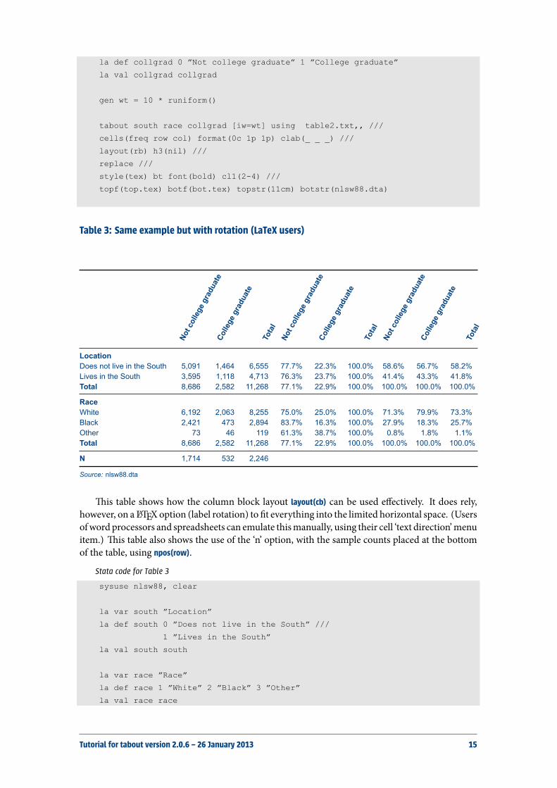
is table shows how the column block layout layout(cb) can be used effectively. It does rely,however, on a LATEXoption (label rotation) to t everything into the limited horizontal space. (Usersofword processors and spreadsheets can emulate thismanually, using their cell ‘text direction’menuitem.) is table also shows the use of the ‘n’ option, with the sample counts placed at the bottomof the table, using npos(row).
Stata code for Table 3
sysuse nlsw88, clear
la var south ”Location”
la def south 0 ”Does not live in the South” ///
1 ”Lives in the South”
la val south south
la var race ”Race”
la def race 1 ”White” 2 ”Black” 3 ”Other”
la val race race
Tutorial for tabout version 2.0.6 – 26 January 2013 15

la var collgrad ”Education”
la def collgrad 0 ”Not college graduate” 1 ”College graduate”
la val collgrad collgrad
gen wt = 10 * runiform()
tabout south race collgrad [iw=wt] using table3.txt, ///
cells(freq row col) format(0c 1p 1p) layout(cb) h1(nil) h3(nil) npos(row) ///
replace ///
style(tex) bt font(bold) rotate(60) ///
topf(top.tex) botf(bot.tex) topstr(15cm) botstr(nlsw88.dta)
LATEX users will need to make sure they have the following block of code in their documentpreamble if they wish to make use of the label rotation option.
LaTeX Code for rotation of table headings
\newcommand{\rot}[2]{\rule{1em}{0pt}%
\makebox[0cm][c]{\rotatebox{#1}{\ #2}}}
Table 4: Same example illustrating noffset option
Not college
graduate
College
graduate
Total
Not college
graduate
College
graduate
Total
Not college
graduate
College
graduate
Total
LocationDoes not live in the South 5,062 1,581 6,643 76.2% 23.8% 100.0% 59.1% 58.5% 58.9%Lives in the South 3,507 1,123 4,630 75.7% 24.3% 100.0% 40.9% 41.5% 41.1%Total 8,569 2,704 11,273 76.0% 24.0% 100.0% 100.0% 100.0% 100.0%
RaceWhite 6,124 2,115 8,239 74.3% 25.7% 100.0% 71.5% 78.2% 73.1%Black 2,353 544 2,898 81.2% 18.8% 100.0% 27.5% 20.1% 25.7%Other 91 45 136 66.8% 33.2% 100.0% 1.1% 1.7% 1.2%Total 8,569 2,704 11,273 76.0% 24.0% 100.0% 100.0% 100.0% 100.0%
N 1,714 532 2,246
Source: nlsw88.dta
is table reproduces the last one, but shows the effect of the noffset option. A common layoutis frequencies rst, then either column or row percentages, so it oen makes more sense to ‘lineup’ the n counts below the column percentages. e noffset option allows you to ‘shi’ the n countsalong to line up under a column (or column block) of your choosing. In this example, the noff(3)shis the n counts into the third block. If you weren’t using the layout(cb) option and allowed thedata to be in alternating columns (eg. freq row col freq row col etc), then the effect of noff(3) wouldbe to place the n counts in the third alternating column: blank blank n blank blank n etc. Keepin mind that noffset refers to the data columns and rows, ignoring labels and headings (since to beprecise, the rst column always has labels in it). If you are using the npos(row) or npos(rb) options,
16 Tutorial for tabout version 2.0.6 – 26 January 2013
the same principles apply (just read ‘row’ instead of ‘column’ in the above explanation). (Note thatfrom here on, I begin to introduce abbreviations for options which have appeared several times.)
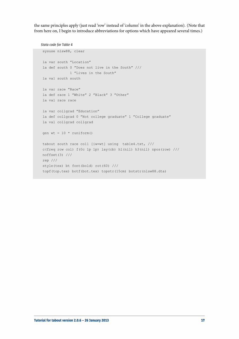
Stata code for Table 4
sysuse nlsw88, clear
la var south ”Location”
la def south 0 ”Does not live in the South” ///
1 ”Lives in the South”
la val south south
la var race ”Race”
la def race 1 ”White” 2 ”Black” 3 ”Other”
la val race race
la var collgrad ”Education”
la def collgrad 0 ”Not college graduate” 1 ”College graduate”
la val collgrad collgrad
gen wt = 10 * runiform()
tabout south race coll [iw=wt] using table4.txt, ///
c(freq row col) f(0c 1p 1p) lay(cb) h1(nil) h3(nil) npos(row) ///
noffset(3) ///
rep ///
style(tex) bt font(bold) rot(60) ///
topf(top.tex) botf(bot.tex) topstr(15cm) botstr(nlsw88.dta)
Tutorial for tabout version 2.0.6 – 26 January 2013 17
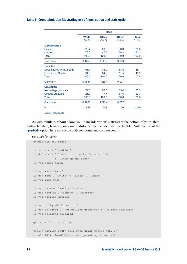
Table 5: Cross tabulation illustrating use of npos option and stats option
Race
White Black Other TotalCol % Col % Col % Col %
Marital statusSingle 29.7 53.0 30.8 35.8Married 70.3 47.0 69.2 64.2Total 100.0 100.0 100.0 100.0
Gamma = -0.4256 ASE = 0.039
LocationDoes not live in the South 65.4 36.0 88.5 58.1Lives in the South 34.6 64.0 11.5 41.9Total 100.0 100.0 100.0 100.0
Gamma = 0.4834 ASE = 0.037
EducationNot college graduate 74.3 82.3 65.4 76.3College graduate 25.7 17.7 34.6 23.7Total 100.0 100.0 100.0 100.0
Gamma = -0.1990 ASE = 0.057
N 1,637 583 26 2,246
Source: nlsw88.dta
As with tabulate, tabout allows you to include various statistics at the bottom of your tables.Unlike tabulate, however, only one statistic can be included with each table. Note the use of thenpos(both) option here to provide both row count and column counts.
Stata code for Table 5
sysuse nlsw88, clear
la var south ”Location”
la def south 0 ”Does not live in the South” ///
1 ”Lives in the South”
la val south south
la var race ”Race”
la def race 1 ”White” 2 ”Black” 3 ”Other”
la val race race
la var married ”Marital status”
la def married 0 ”Single” 1 ”Married”
la val married married
la var collgrad ”Education”
la def collgrad 0 ”Not college graduate” 1 ”College graduate”
la val collgrad collgrad
gen wt = 10 * runiform()
tabout married south coll race using table5.txt, ///
c(col) f(1) clab(Col_%) stats(gamma) npos(row) ///
18 Tutorial for tabout version 2.0.6 – 26 January 2013
rep ///
style(tex) bt font(bold) cl1(2-5) ///
topf(top.tex) botf(bot.tex) topstr(11cm) botstr(nlsw88.dta)
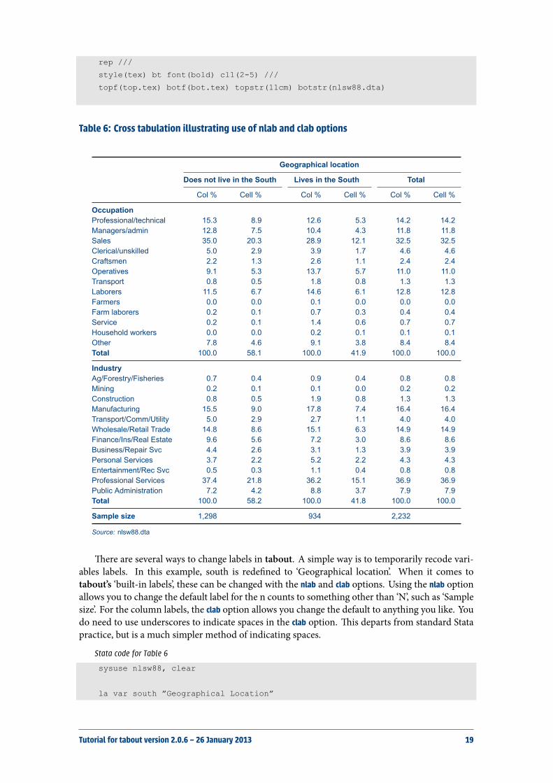
Table 6: Cross tabulation illustrating use of nlab and clab options
Geographical location
Does not live in the South Lives in the South Total
Col % Cell % Col % Cell % Col % Cell %
OccupationProfessional/technical 15.3 8.9 12.6 5.3 14.2 14.2Managers/admin 12.8 7.5 10.4 4.3 11.8 11.8Sales 35.0 20.3 28.9 12.1 32.5 32.5Clerical/unskilled 5.0 2.9 3.9 1.7 4.6 4.6Craftsmen 2.2 1.3 2.6 1.1 2.4 2.4Operatives 9.1 5.3 13.7 5.7 11.0 11.0Transport 0.8 0.5 1.8 0.8 1.3 1.3Laborers 11.5 6.7 14.6 6.1 12.8 12.8Farmers 0.0 0.0 0.1 0.0 0.0 0.0Farm laborers 0.2 0.1 0.7 0.3 0.4 0.4Service 0.2 0.1 1.4 0.6 0.7 0.7Household workers 0.0 0.0 0.2 0.1 0.1 0.1Other 7.8 4.6 9.1 3.8 8.4 8.4Total 100.0 58.1 100.0 41.9 100.0 100.0
IndustryAg/Forestry/Fisheries 0.7 0.4 0.9 0.4 0.8 0.8Mining 0.2 0.1 0.1 0.0 0.2 0.2Construction 0.8 0.5 1.9 0.8 1.3 1.3Manufacturing 15.5 9.0 17.8 7.4 16.4 16.4Transport/Comm/Utility 5.0 2.9 2.7 1.1 4.0 4.0Wholesale/Retail Trade 14.8 8.6 15.1 6.3 14.9 14.9Finance/Ins/Real Estate 9.6 5.6 7.2 3.0 8.6 8.6Business/Repair Svc 4.4 2.6 3.1 1.3 3.9 3.9Personal Services 3.7 2.2 5.2 2.2 4.3 4.3Entertainment/Rec Svc 0.5 0.3 1.1 0.4 0.8 0.8Professional Services 37.4 21.8 36.2 15.1 36.9 36.9Public Administration 7.2 4.2 8.8 3.7 7.9 7.9Total 100.0 58.2 100.0 41.8 100.0 100.0
Sample size 1,298 934 2,232
Source: nlsw88.dta
ere are several ways to change labels in tabout. A simple way is to temporarily recode vari-ables labels. In this example, south is rede ned to ‘Geographical location’. When it comes totabout’s ‘built-in labels’, these can be changed with the nlab and clab options. Using the nlab optionallows you to change the default label for the n counts to something other than ‘N’, such as ‘Samplesize’. For the column labels, the clab option allows you change the default to anything you like. Youdo need to use underscores to indicate spaces in the clab option. is departs from standard Statapractice, but is a much simpler method of indicating spaces.
Stata code for Table 6
sysuse nlsw88, clear
la var south ”Geographical Location”
Tutorial for tabout version 2.0.6 – 26 January 2013 19

la def south 0 ”Does not live in the South” ///
1 ”Lives in the South”
la val south south
la var industry ”Industry”
la var occupation ”Occupation”
tabout occupation industry south using table6.txt, ///
c(col cell) f(1) clab(Col_% Cell_%) npos(row) nlab(Sample size) ///
rep ///
style(tex) bt font(bold) cl1(2-7) cl2(2-3 4-5 6-7) ///
topf(top.tex) botf(bot.tex) topstr(14cm) botstr(nlsw88.dta)
Table 7: Same table illustrating column block layout option (cb) and dpcomma option
Location
Does notlive in the
South
Lives inthe South
Total Does notlive in the
South
Lives inthe South
Total
Column percentages Cell percentages
OccupationProfessional/technical 15,3 12,6 14,2 8,9 5,3 14,2Managers/admin 12,8 10,4 11,8 7,5 4,3 11,8Sales 35,0 28,9 32,5 20,3 12,1 32,5Clerical/unskilled 5,0 3,9 4,6 2,9 1,7 4,6Craftsmen 2,2 2,6 2,4 1,3 1,1 2,4Operatives 9,1 13,7 11,0 5,3 5,7 11,0Transport 0,8 1,8 1,3 0,5 0,8 1,3Laborers 11,5 14,6 12,8 6,7 6,1 12,8Farmers 0,0 0,1 0,0 0,0 0,0 0,0Farm laborers 0,2 0,7 0,4 0,1 0,3 0,4Service 0,2 1,4 0,7 0,1 0,6 0,7Household workers 0,0 0,2 0,1 0,0 0,1 0,1Other 7,8 9,1 8,4 4,6 3,8 8,4Total 100,0 100,0 100,0 58,1 41,9 100,0
IndustryAg/Forestry/Fisheries 0,7 0,9 0,8 0,4 0,4 0,8Mining 0,2 0,1 0,2 0,1 0,0 0,2Construction 0,8 1,9 1,3 0,5 0,8 1,3Manufacturing 15,5 17,8 16,4 9,0 7,4 16,4Transport/Comm/Utility 5,0 2,7 4,0 2,9 1,1 4,0Wholesale/Retail Trade 14,8 15,1 14,9 8,6 6,3 14,9Finance/Ins/Real Estate 9,6 7,2 8,6 5,6 3,0 8,6Business/Repair Svc 4,4 3,1 3,9 2,6 1,3 3,9Personal Services 3,7 5,2 4,3 2,2 2,2 4,3Entertainment/Rec Svc 0,5 1,1 0,8 0,3 0,4 0,8Professional Services 37,4 36,2 36,9 21,8 15,1 36,9Public Administration 7,2 8,8 7,9 4,2 3,7 7,9Total 100,0 100,0 100,0 58,2 41,8 100,0
Sample size 1.298 934 2.232
Source: nlsw88.dta
While Table 6 looks neat, cell percentages are more easily grasped as a block, so Table 7 duplic-ates the that table, but changes the layout to column block (layout(cb)). e table also illustrates one
20 Tutorial for tabout version 2.0.6 – 26 January 2013
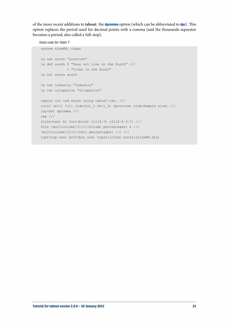
of the more recent additions to tabout: the dpcomma option (which can be abbreviated to dpc). isoption replaces the period used for decimal points with a comma (and the thousands separatorbecomes a period, also called a full-stop).
Stata code for Table 7
sysuse nlsw88, clear
la var south ”Location”
la def south 0 ”Does not live in the South” ///
1 ”Lives in the South”
la val south south
la var industry ”Industry”
la var occupation ”Occupation”
tabout occ ind south using table7.txt, ///
c(col cell) f(1) clab(Col_% Cell_%) npos(row) nlab(Sample size) ///
lay(cb) dpcomma ///
rep ///
style(tex) bt font(bold) cl1(2-7) cl2(2-4 5-7) ///
h3(& \multicolumn{3}{c}{Column percentages} & ///
\multicolumn{3}{c}{Cell percentages} \\) ///
topf(top.tex) botf(bot.tex) topstr(13cm) botstr(nlsw88.dta)
Tutorial for tabout version 2.0.6 – 26 January 2013 21
Basic tables with survey data
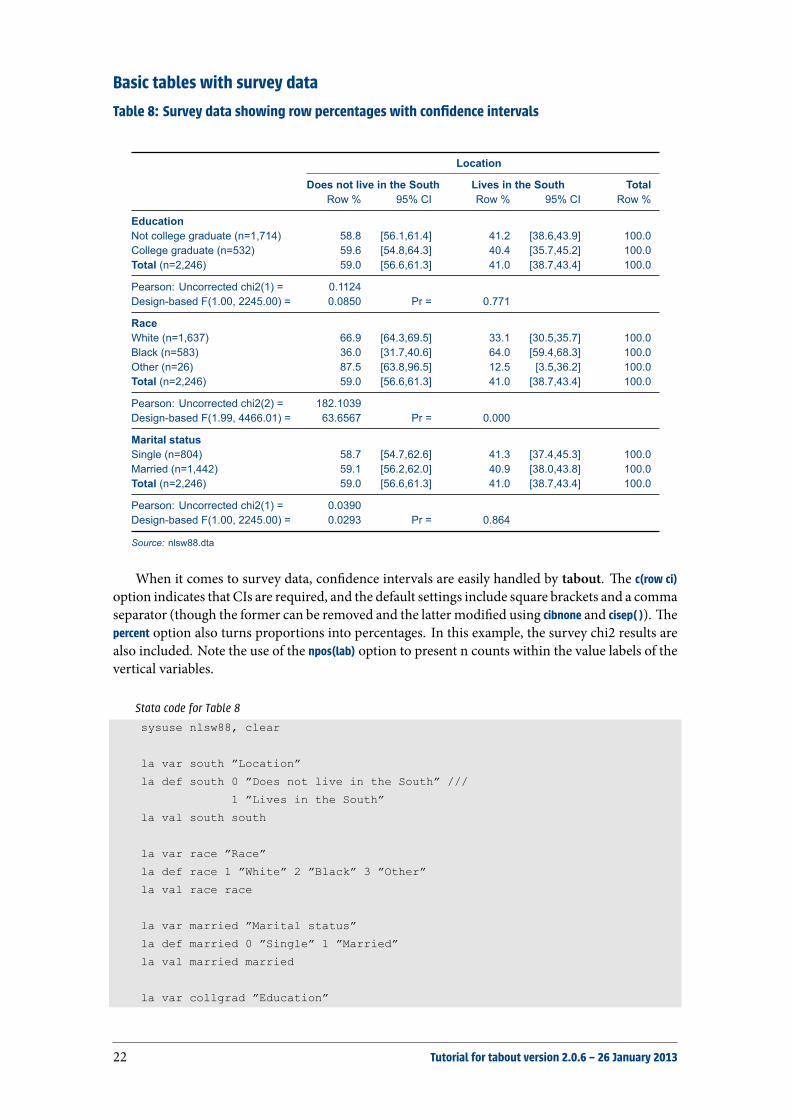
Table 8: Survey data showing row percentages with confidence intervals
Location
Does not live in the South Lives in the South TotalRow % 95% CI Row % 95% CI Row %
EducationNot college graduate (n=1,714) 58.8 [56.1,61.4] 41.2 [38.6,43.9] 100.0College graduate (n=532) 59.6 [54.8,64.3] 40.4 [35.7,45.2] 100.0Total (n=2,246) 59.0 [56.6,61.3] 41.0 [38.7,43.4] 100.0
Pearson: Uncorrected chi2(1) = 0.1124Design-based F(1.00, 2245.00) = 0.0850 Pr = 0.771
RaceWhite (n=1,637) 66.9 [64.3,69.5] 33.1 [30.5,35.7] 100.0Black (n=583) 36.0 [31.7,40.6] 64.0 [59.4,68.3] 100.0Other (n=26) 87.5 [63.8,96.5] 12.5 [3.5,36.2] 100.0Total (n=2,246) 59.0 [56.6,61.3] 41.0 [38.7,43.4] 100.0
Pearson: Uncorrected chi2(2) = 182.1039Design-based F(1.99, 4466.01) = 63.6567 Pr = 0.000
Marital statusSingle (n=804) 58.7 [54.7,62.6] 41.3 [37.4,45.3] 100.0Married (n=1,442) 59.1 [56.2,62.0] 40.9 [38.0,43.8] 100.0Total (n=2,246) 59.0 [56.6,61.3] 41.0 [38.7,43.4] 100.0
Pearson: Uncorrected chi2(1) = 0.0390Design-based F(1.00, 2245.00) = 0.0293 Pr = 0.864
Source: nlsw88.dta
When it comes to survey data, con dence intervals are easily handled by tabout. e c(row ci)option indicates that CIs are required, and the default settings include square brackets and a commaseparator (though the former can be removed and the latter modi ed using cibnone and cisep( )). epercent option also turns proportions into percentages. In this example, the survey chi2 results arealso included. Note the use of the npos(lab) option to present n counts within the value labels of thevertical variables.
Stata code for Table 8
sysuse nlsw88, clear
la var south ”Location”
la def south 0 ”Does not live in the South” ///
1 ”Lives in the South”
la val south south
la var race ”Race”
la def race 1 ”White” 2 ”Black” 3 ”Other”
la val race race
la var married ”Marital status”
la def married 0 ”Single” 1 ”Married”
la val married married
la var collgrad ”Education”
22 Tutorial for tabout version 2.0.6 – 26 January 2013
la def collgrad 0 ”Not college graduate” 1 ”College graduate”
la val collgrad collgrad
gen wt = 10 * runiform()
svyset [pw=wt]
tabout coll race married south using table8.txt, ///
c(row ci) f(1 1) clab(Row_% 95%_CI) svy stats(chi2) ///
npos(lab) percent ///
rep ///
style(tex) bt font(bold) cl1(2-6) ///
topf(top.tex) botf(bot.tex) topstr(14cm) botstr(nlsw88.dta)
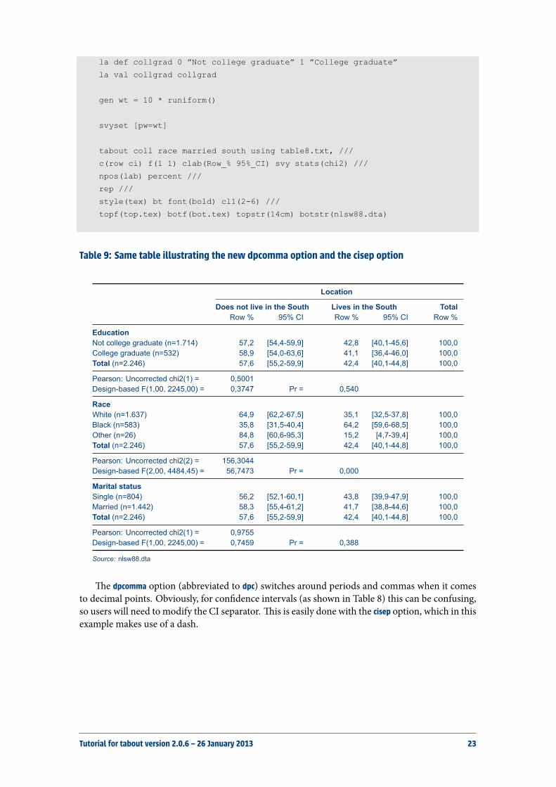
Table 9: Same table illustrating the new dpcomma option and the cisep option
Location
Does not live in the South Lives in the South TotalRow % 95% CI Row % 95% CI Row %
EducationNot college graduate (n=1.714) 57,2 [54,4-59,9] 42,8 [40,1-45,6] 100,0College graduate (n=532) 58,9 [54,0-63,6] 41,1 [36,4-46,0] 100,0Total (n=2.246) 57,6 [55,2-59,9] 42,4 [40,1-44,8] 100,0
Pearson: Uncorrected chi2(1) = 0,5001Design-based F(1,00, 2245,00) = 0,3747 Pr = 0,540
RaceWhite (n=1.637) 64,9 [62,2-67,5] 35,1 [32,5-37,8] 100,0Black (n=583) 35,8 [31,5-40,4] 64,2 [59,6-68,5] 100,0Other (n=26) 84,8 [60,6-95,3] 15,2 [4,7-39,4] 100,0Total (n=2.246) 57,6 [55,2-59,9] 42,4 [40,1-44,8] 100,0
Pearson: Uncorrected chi2(2) = 156,3044Design-based F(2,00, 4484,45) = 56,7473 Pr = 0,000
Marital statusSingle (n=804) 56,2 [52,1-60,1] 43,8 [39,9-47,9] 100,0Married (n=1.442) 58,3 [55,4-61,2] 41,7 [38,8-44,6] 100,0Total (n=2.246) 57,6 [55,2-59,9] 42,4 [40,1-44,8] 100,0
Pearson: Uncorrected chi2(1) = 0,9755Design-based F(1,00, 2245,00) = 0,7459 Pr = 0,388
Source: nlsw88.dta
e dpcomma option (abbreviated to dpc) switches around periods and commas when it comesto decimal points. Obviously, for con dence intervals (as shown in Table 8) this can be confusing,so users will need to modify the CI separator. is is easily done with the cisep option, which in thisexample makes use of a dash.
Tutorial for tabout version 2.0.6 – 26 January 2013 23
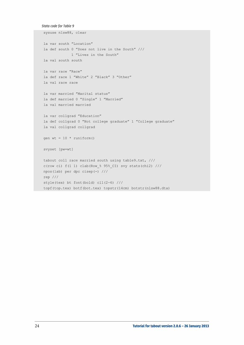
Stata code for Table 9
sysuse nlsw88, clear
la var south ”Location”
la def south 0 ”Does not live in the South” ///
1 ”Lives in the South”
la val south south
la var race ”Race”
la def race 1 ”White” 2 ”Black” 3 ”Other”
la val race race
la var married ”Marital status”
la def married 0 ”Single” 1 ”Married”
la val married married
la var collgrad ”Education”
la def collgrad 0 ”Not college graduate” 1 ”College graduate”
la val collgrad collgrad
gen wt = 10 * runiform()
svyset [pw=wt]
tabout coll race married south using table9.txt, ///
c(row ci) f(1 1) clab(Row_% 95%_CI) svy stats(chi2) ///
npos(lab) per dpc cisep(-) ///
rep ///
style(tex) bt font(bold) cl1(2-6) ///
topf(top.tex) botf(bot.tex) topstr(14cm) botstr(nlsw88.dta)
24 Tutorial for tabout version 2.0.6 – 26 January 2013

Summary tablesSummary tables in tabout can be as simple as the following table, where two variables (inc and can-didate) are cross-tabulated and the cell contents are based on the mean of another variable (pfrac).is is essentially the same as Stata’s table command. Note that the sum option is required to indic-ate that this is a summary table.
Table 10: Simple twoway summary table illustrating a table of means
Candidate voted for, 1992
Family Income Clinton Bush Perot Total% % % %
<$15k 8.3 3.2 2.5 4.7$15-30k 10.8 8.4 4.8 8.0$30-50k 12.3 11.4 6.3 10.0$50-75k 8.0 8.4 3.6 6.7$75k+ 4.7 6.2 2.1 4.3Total 8.8 7.5 3.9 6.7
Source: voter.dta
Stata code for Table 10
sysuse voter, clear
tabout inc candidat using table10.txt, ///
c(mean pfrac) f(1) clab(%) sum ///
rep ///
style(tex) bt font(bold) cl1(2-5) ///
topf(top.tex) botf(bot.tex) topstr(12cm) botstr(voter.dta)
Table 11: Twoway summary table illustrating inter-quartile range
Inter-quartile range of weight
Repair Record 1978 Domestic Foreign Total N
1 3,100 3,100 22 3,354 3,354 83 3,442 2,010 3,299 304 3,532 2,208 2,870 185 1,960 2,403 2,323 11Total 3,368 2,263 3,032 69
N 48 21 69
Source: auto.dta
Table 11 shows another example of a summary table, in this case the inter-quartile range. Asmentioned earlier, this is but one of a large number of possible summary measures available withthis option: N mean var sd skewness kurtosis sum uwsum min max count median iqr r9010 r9050r7525 r1050 p1 p5 p10 p25 p50 p75 p90 p95 p99. Note that tabout works out that this is a twowaytable and uses the last variable in the list (foreign) as the ‘horizontal’ variable.
Tutorial for tabout version 2.0.6 – 26 January 2013 25
Stata code for Table 11
sysuse auto, clear
tabout rep78 foreign using table11.txt, ///
c(mean weight) f(0c) sum h3(nil) npos(both) ///
rep ///
style(tex) bt font(bold) cl1(2-4) cltr1(.5em) ///
h1(& \multicolumn{3}{c}{\textbf{Inter-quartile range of weight}} \\) ///
topf(top.tex) botf(bot.tex) topstr(10cm) botstr(auto.dta)
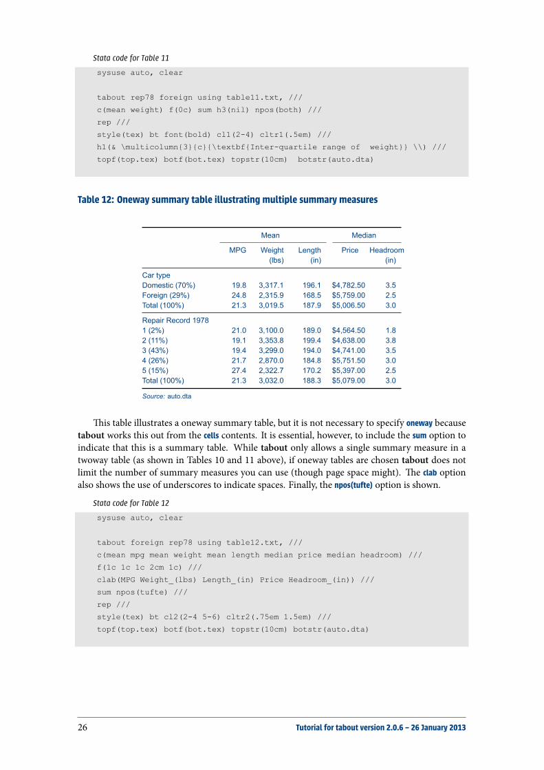
Table 12: Oneway summary table illustrating multiple summary measures
Mean Median
MPG Weight(lbs)
Length(in)
Price Headroom(in)
Car typeDomestic (70%) 19.8 3,317.1 196.1 $4,782.50 3.5Foreign (29%) 24.8 2,315.9 168.5 $5,759.00 2.5Total (100%) 21.3 3,019.5 187.9 $5,006.50 3.0
Repair Record 19781 (2%) 21.0 3,100.0 189.0 $4,564.50 1.82 (11%) 19.1 3,353.8 199.4 $4,638.00 3.83 (43%) 19.4 3,299.0 194.0 $4,741.00 3.54 (26%) 21.7 2,870.0 184.8 $5,751.50 3.05 (15%) 27.4 2,322.7 170.2 $5,397.00 2.5Total (100%) 21.3 3,032.0 188.3 $5,079.00 3.0
Source: auto.dta
is table illustrates a oneway summary table, but it is not necessary to specify oneway becausetabout works this out from the cells contents. It is essential, however, to include the sum option toindicate that this is a summary table. While tabout only allows a single summary measure in atwoway table (as shown in Tables 10 and 11 above), if oneway tables are chosen tabout does notlimit the number of summary measures you can use (though page space might). e clab optionalso shows the use of underscores to indicate spaces. Finally, the npos(tufte) option is shown.
Stata code for Table 12
sysuse auto, clear
tabout foreign rep78 using table12.txt, ///
c(mean mpg mean weight mean length median price median headroom) ///
f(1c 1c 1c 2cm 1c) ///
clab(MPG Weight_(lbs) Length_(in) Price Headroom_(in)) ///
sum npos(tufte) ///
rep ///
style(tex) bt cl2(2-4 5-6) cltr2(.75em 1.5em) ///
topf(top.tex) botf(bot.tex) topstr(10cm) botstr(auto.dta)
26 Tutorial for tabout version 2.0.6 – 26 January 2013
Summary tables with survey data
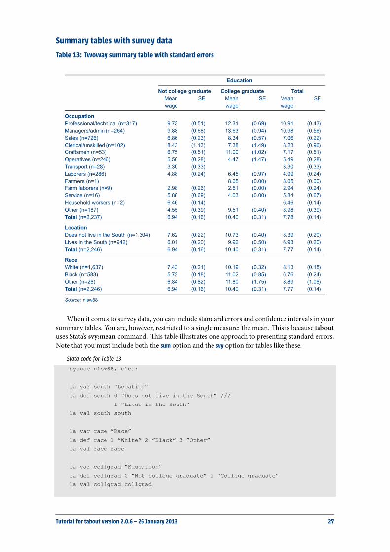
Table 13: Twoway summary table with standard errors
Education
Not college graduate College graduate TotalMeanwage
SE Meanwage
SE Meanwage
SE
OccupationProfessional/technical (n=317) 9.73 (0.51) 12.31 (0.69) 10.91 (0.43)Managers/admin (n=264) 9.88 (0.68) 13.63 (0.94) 10.98 (0.56)Sales (n=726) 6.86 (0.23) 8.34 (0.57) 7.06 (0.22)Clerical/unskilled (n=102) 8.43 (1.13) 7.38 (1.49) 8.23 (0.96)Craftsmen (n=53) 6.75 (0.51) 11.00 (1.02) 7.17 (0.51)Operatives (n=246) 5.50 (0.28) 4.47 (1.47) 5.49 (0.28)Transport (n=28) 3.30 (0.33) 3.30 (0.33)Laborers (n=286) 4.88 (0.24) 6.45 (0.97) 4.99 (0.24)Farmers (n=1) 8.05 (0.00) 8.05 (0.00)Farm laborers (n=9) 2.98 (0.26) 2.51 (0.00) 2.94 (0.24)Service (n=16) 5.88 (0.69) 4.03 (0.00) 5.84 (0.67)Household workers (n=2) 6.46 (0.14) 6.46 (0.14)Other (n=187) 4.55 (0.39) 9.51 (0.40) 8.98 (0.39)Total (n=2,237) 6.94 (0.16) 10.40 (0.31) 7.78 (0.14)
LocationDoes not live in the South (n=1,304) 7.62 (0.22) 10.73 (0.40) 8.39 (0.20)Lives in the South (n=942) 6.01 (0.20) 9.92 (0.50) 6.93 (0.20)Total (n=2,246) 6.94 (0.16) 10.40 (0.31) 7.77 (0.14)
RaceWhite (n=1,637) 7.43 (0.21) 10.19 (0.32) 8.13 (0.18)Black (n=583) 5.72 (0.18) 11.02 (0.85) 6.76 (0.24)Other (n=26) 6.84 (0.82) 11.80 (1.75) 8.89 (1.06)Total (n=2,246) 6.94 (0.16) 10.40 (0.31) 7.77 (0.14)
Source: nlsw88
When it comes to survey data, you can include standard errors and con dence intervals in yoursummary tables. You are, however, restricted to a single measure: the mean. is is because taboutuses Stata’s svy:mean command. is table illustrates one approach to presenting standard errors.Note that you must include both the sum option and the svy option for tables like these.
Stata code for Table 13
sysuse nlsw88, clear
la var south ”Location”
la def south 0 ”Does not live in the South” ///
1 ”Lives in the South”
la val south south
la var race ”Race”
la def race 1 ”White” 2 ”Black” 3 ”Other”
la val race race
la var collgrad ”Education”
la def collgrad 0 ”Not college graduate” 1 ”College graduate”
la val collgrad collgrad
Tutorial for tabout version 2.0.6 – 26 January 2013 27
la var occupation ”Occupation”
gen wt = 10 * runiform()
svyset [pw=wt]
tabout occ south race coll using table13.txt, ///
c(mean wage se) f(2 2) clab(Mean_wage SE) ///
sum svy npos(lab) ///
rep ///
style(tex) bt cl1(2-7) font(bold) ///
topf(top.tex) botf(bot.tex) topstr(14cm) botstr(nlsw88)
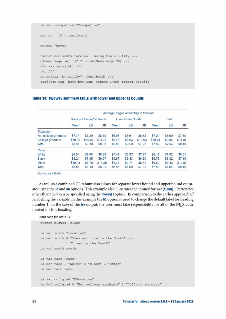
Table 14: Twoway summary table with lower and upper CI bounds
Average wages according to location
Does not live in the South Lives in the South Total
Mean LB UB Mean LB UB Mean LB UB
EducationNot college graduate $7.74 $7.29 $8.19 $5.96 $5.61 $6.32 $7.00 $6.69 $7.30College graduate $10.90 $10.07 $11.72 $9.78 $8.93 $10.63 $10.44 $9.84 $11.05Total $8.51 $8.10 $8.91 $6.85 $6.50 $7.21 $7.82 $7.54 $8.10
RaceWhite $8.54 $8.08 $8.99 $7.47 $6.97 $7.97 $8.17 $7.82 $8.51Black $8.21 $7.35 $9.07 $5.87 $5.43 $6.30 $6.76 $6.32 $7.19Other $10.03 $6.79 $13.28 $4.73 $0.74 $8.71 $9.50 $6.43 $12.57Total $8.51 $8.10 $8.91 $6.85 $6.50 $7.21 $7.82 $7.54 $8.10
Source: nlsw88.dta
As well as a combined CI, tabout also allows for separate lower bound and upper bound estim-ates using the lb and ub options. is example also illustrates the money format (f(2m)). Currenciesother than the $ can be speci ed using the money( ) option. In comparison to the earlier approach ofrelabelling the variable, in this example the h1 option is used to change the default label for headingnumber 1. In the case of the tex output, the user must take responsibility for all of the LATEX codeneeded for this heading.
Stata code for Table 14
sysuse nlsw88, clear
la var south ”Location”
la def south 0 ”Does not live in the South” ///
1 ”Lives in the South”
la val south south
la var race ”Race”
la def race 1 ”White” 2 ”Black” 3 ”Other”
la val race race
la var collgrad ”Education”
la def collgrad 0 ”Not college graduate” 1 ”College graduate”
28 Tutorial for tabout version 2.0.6 – 26 January 2013

la val collgrad collgrad
gen wt = 10 * runiform()
svyset [pw=wt]
tabout coll race south using table14.txt, ///
c(mean wage lb ub) f(2m) svy sum ///
rep ///
style(tex) bt font(italic) cl1(2-10) cl2(2-4 5-7 8-10) ///
h1(& \multicolumn{9}{c}{\emph{Average wages according to location}} \\) ///
topf(top.tex) botf(bot.tex) topstr(14cm) botstr(nlsw88.dta)
Table 15: Twoway summary table with standard errors and CIs in row layout
Location
Does not live inthe South
Lives in theSouth
Total
Average wage
EducationNot college graduate (n=1,714) 7.74 6.01 6.98(SE) (0.21) (0.20) (0.15)(90% CI) [7.39,8.09] [5.68,6.33] [6.73,7.22]College graduate (n=532) 10.98 10.12 10.63(SE) (0.42) (0.48) (0.32)(90% CI) [10.29,11.66] [9.33,10.92] [10.11,11.15]Total (n=2,246) 8.55 6.93 7.85(SE) (0.19) (0.20) (0.14)(90% CI) [8.23,8.87] [6.60,7.26] [7.62,8.08]
RaceWhite (n=1,637) 8.54 7.59 8.20(SE) (0.22) (0.27) (0.17)(90% CI) [8.18,8.90] [7.14,8.04] [7.92,8.48]Black (n=583) 8.56 5.87 6.86(SE) (0.45) (0.26) (0.24)(90% CI) [7.81,9.30] [5.44,6.30] [6.46,7.26]Other (n=26) 8.71 8.89 8.73(SE) (1.38) (2.36) (1.27)(90% CI) [6.45,10.98] [5.01,12.76] [6.63,10.82]Total (n=2,246) 8.55 6.93 7.85(SE) (0.19) (0.20) (0.14)(90% CI) [8.23,8.87] [6.60,7.26] [7.62,8.08]
Source: nlsw88.dta
is table shows similar data, but with the layout designated as row. e level option (abbre-viated to l) is inherited from Stata’s survey commands and sets the con dence interval level. edefault is 95%, so the option can usually be le out since this default is a very common one. Here,for purposes of illustration, the level has been changed to 90%, using level(90).
Note the use of the rst underscore in clab(_ (SE) (90%_CI) to indicate an empty label. is suitsrow layout where the value labels for the ‘vertical’ variables occupy the main part of the rst row.Notice also the use of the h3 option to place useful information above the data in the table. Normally,
Tutorial for tabout version 2.0.6 – 26 January 2013 29
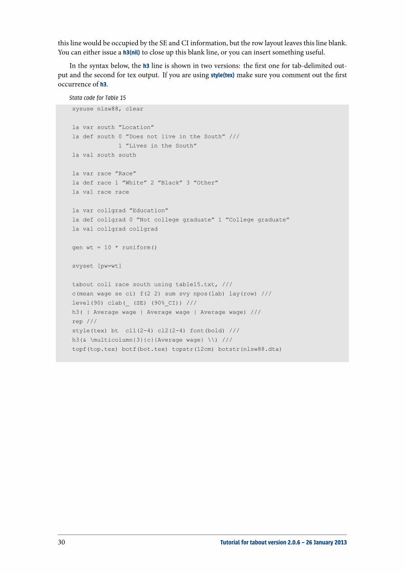
this line would be occupied by the SE and CI information, but the row layout leaves this line blank.You can either issue a h3(nil) to close up this blank line, or you can insert something useful.
In the syntax below, the h3 line is shown in two versions: the rst one for tab-delimited out-put and the second for tex output. If you are using style(tex) make sure you comment out the rstoccurrence of h3.
Stata code for Table 15
sysuse nlsw88, clear
la var south ”Location”
la def south 0 ”Does not live in the South” ///
1 ”Lives in the South”
la val south south
la var race ”Race”
la def race 1 ”White” 2 ”Black” 3 ”Other”
la val race race
la var collgrad ”Education”
la def collgrad 0 ”Not college graduate” 1 ”College graduate”
la val collgrad collgrad
gen wt = 10 * runiform()
svyset [pw=wt]
tabout coll race south using table15.txt, ///
c(mean wage se ci) f(2 2) sum svy npos(lab) lay(row) ///
level(90) clab(_ (SE) (90%_CI)) ///
h3( | Average wage | Average wage | Average wage) ///
rep ///
style(tex) bt cl1(2-4) cl2(2-4) font(bold) ///
h3(& \multicolumn{3}{c}{Average wage} \\) ///
topf(top.tex) botf(bot.tex) topstr(12cm) botstr(nlsw88.dta)
30 Tutorial for tabout version 2.0.6 – 26 January 2013
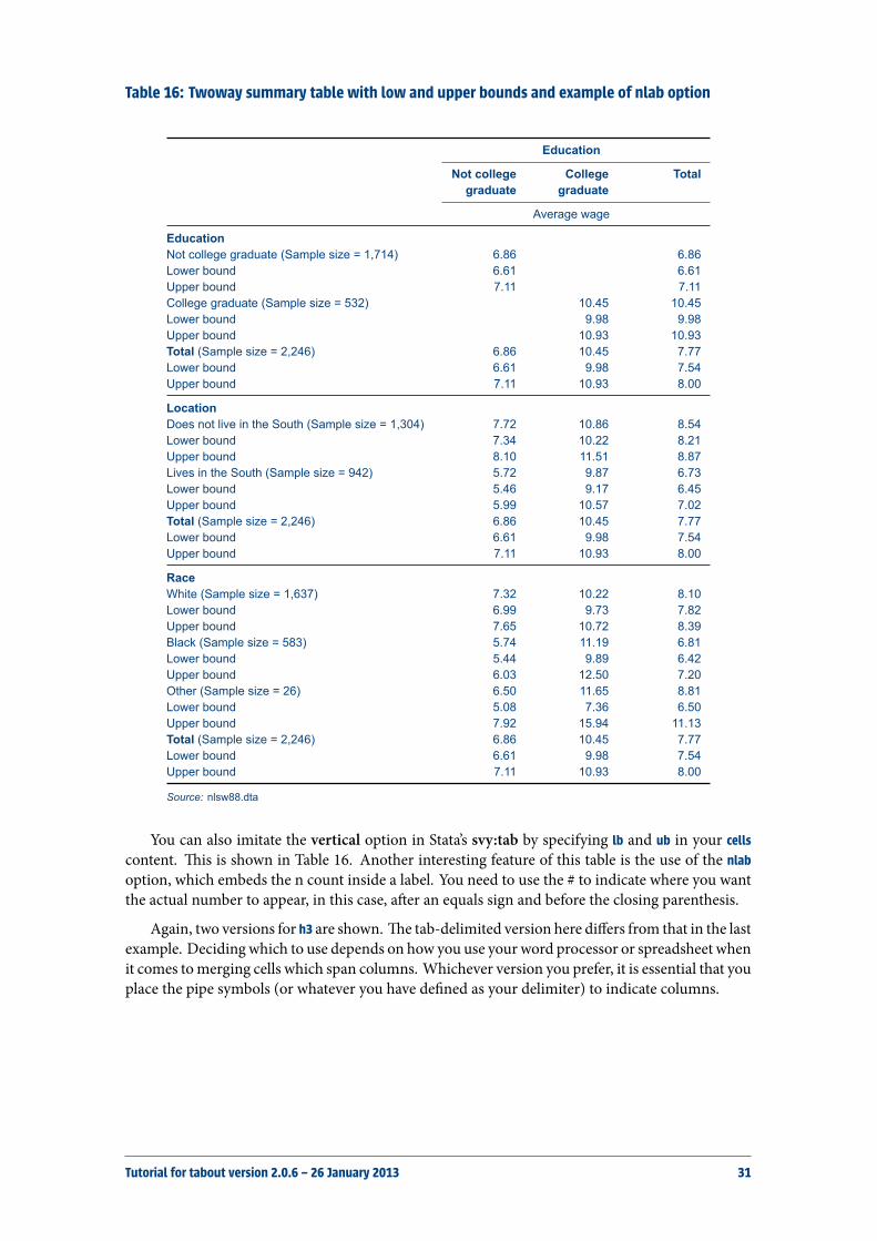
Table 16: Twoway summary table with low and upper bounds and example of nlab option
Education
Not collegegraduate
Collegegraduate
Total
Average wage
EducationNot college graduate (Sample size = 1,714) 6.86 6.86Lower bound 6.61 6.61Upper bound 7.11 7.11College graduate (Sample size = 532) 10.45 10.45Lower bound 9.98 9.98Upper bound 10.93 10.93Total (Sample size = 2,246) 6.86 10.45 7.77Lower bound 6.61 9.98 7.54Upper bound 7.11 10.93 8.00
LocationDoes not live in the South (Sample size = 1,304) 7.72 10.86 8.54Lower bound 7.34 10.22 8.21Upper bound 8.10 11.51 8.87Lives in the South (Sample size = 942) 5.72 9.87 6.73Lower bound 5.46 9.17 6.45Upper bound 5.99 10.57 7.02Total (Sample size = 2,246) 6.86 10.45 7.77Lower bound 6.61 9.98 7.54Upper bound 7.11 10.93 8.00
RaceWhite (Sample size = 1,637) 7.32 10.22 8.10Lower bound 6.99 9.73 7.82Upper bound 7.65 10.72 8.39Black (Sample size = 583) 5.74 11.19 6.81Lower bound 5.44 9.89 6.42Upper bound 6.03 12.50 7.20Other (Sample size = 26) 6.50 11.65 8.81Lower bound 5.08 7.36 6.50Upper bound 7.92 15.94 11.13Total (Sample size = 2,246) 6.86 10.45 7.77Lower bound 6.61 9.98 7.54Upper bound 7.11 10.93 8.00
Source: nlsw88.dta
You can also imitate the vertical option in Stata’s svy:tab by specifying lb and ub in your cellscontent. is is shown in Table 16. Another interesting feature of this table is the use of the nlaboption, which embeds the n count inside a label. You need to use the # to indicate where you wantthe actual number to appear, in this case, aer an equals sign and before the closing parenthesis.
Again, two versions for h3 are shown. e tab-delimited version here differs from that in the lastexample. Deciding which to use depends on how you use your word processor or spreadsheet whenit comes tomerging cells which span columns. Whichever version you prefer, it is essential that youplace the pipe symbols (or whatever you have de ned as your delimiter) to indicate columns.
Tutorial for tabout version 2.0.6 – 26 January 2013 31
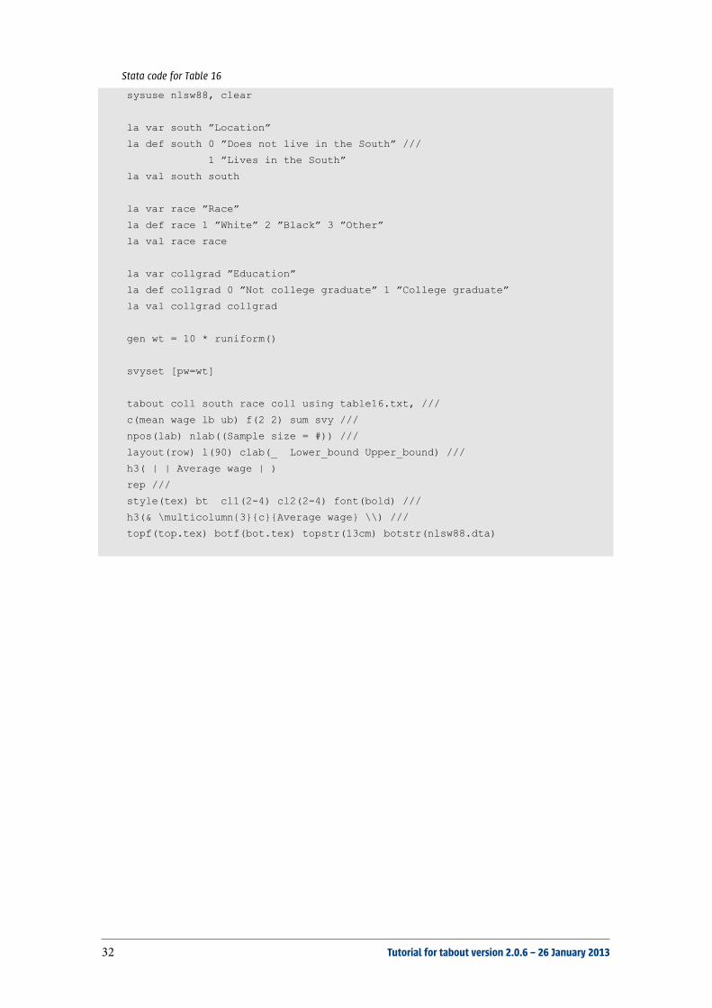
Stata code for Table 16
sysuse nlsw88, clear
la var south ”Location”
la def south 0 ”Does not live in the South” ///
1 ”Lives in the South”
la val south south
la var race ”Race”
la def race 1 ”White” 2 ”Black” 3 ”Other”
la val race race
la var collgrad ”Education”
la def collgrad 0 ”Not college graduate” 1 ”College graduate”
la val collgrad collgrad
gen wt = 10 * runiform()
svyset [pw=wt]
tabout coll south race coll using table16.txt, ///
c(mean wage lb ub) f(2 2) sum svy ///
npos(lab) nlab((Sample size = #)) ///
layout(row) l(90) clab(_ Lower_bound Upper_bound) ///
h3( | | Average wage | )
rep ///
style(tex) bt cl1(2-4) cl2(2-4) font(bold) ///
h3(& \multicolumn{3}{c}{Average wage} \\) ///
topf(top.tex) botf(bot.tex) topstr(13cm) botstr(nlsw88.dta)
32 Tutorial for tabout version 2.0.6 – 26 January 2013
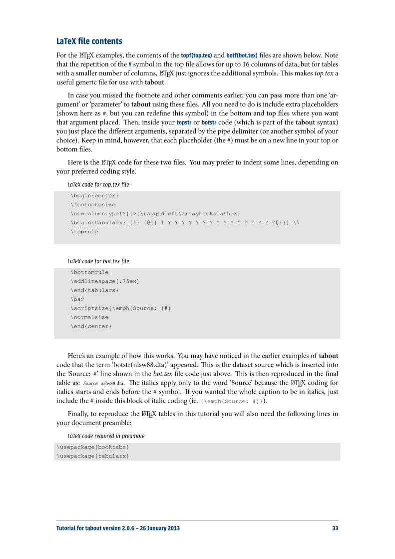
LaTeX file contentsFor the LATEX examples, the contents of the topf(top.tex) and botf(bot.tex) les are shown below. Notethat the repetition of the Y symbol in the top le allows for up to 16 columns of data, but for tableswith a smaller number of columns, LATEX just ignores the additional symbols. is makes top.tex auseful generic le for use with tabout.
In case you missed the footnote and other comments earlier, you can pass more than one ‘ar-gument’ or ‘parameter’ to tabout using these les. All you need to do is include extra placeholders(shown here as #, but you can rede ne this symbol) in the bottom and top les where you wantthat argument placed. en, inside your topstr or botstr code (which is part of the tabout syntax)you just place the different arguments, separated by the pipe delimiter (or another symbol of yourchoice). Keep in mind, however, that each placeholder (the #) must be on a new line in your top orbottom les.
Here is the LATEX code for these two les. You may prefer to indent some lines, depending onyour preferred coding style.
LaTeX code for top.tex file
\begin{center}
\footnotesize
\newcolumntype{Y}{>{\raggedleft\arraybackslash}X}
\begin{tabularx} {#} {@{} l Y Y Y Y Y Y Y Y Y Y Y Y Y Y Y Y@{}} \\
\toprule
LaTeX code for bot.tex file
\bottomrule
\addlinespace[.75ex]
\end{tabularx}
\par
\scriptsize{\emph{Source: }#}
\normalsize
\end{center}
Here’s an example of how this works. You may have noticed in the earlier examples of taboutcode that the term ‘botstr(nlsw88.dta)’ appeared. is is the dataset source which is inserted intothe ‘Source: #’ line shown in the bot.tex le code just above. is is then reproduced in the naltable as: Source: nslw88.dta. e italics apply only to the word ‘Source’ because the LATEX coding foritalics starts and ends before the # symbol. If you wanted the whole caption to be in italics, justinclude the # inside this block of italic coding (ie. {\emph{Source: #}}).
Finally, to reproduce the LATEX tables in this tutorial you will also need the following lines inyour document preamble:
LaTeX code required in preamble
\usepackage{booktabs}
\usepackage{tabularx}
Tutorial for tabout version 2.0.6 – 26 January 2013 33

Tips and Tricks
Three-way tables with tabout?Here is the type of table which this trick produces, a cross-tabulation of union member by industryby race:
Member of a union
Industry Not in union In union Total
Race: whiteAg/Forestry/Fisheries 8 1 9Mining 2 0 2Construction 14 2 16Manufacturing 155 40 195Transport/Comm/Utility 31 28 59Wholesale/Retail Trade 188 18 206Finance/Ins/Real Estate 127 6 133Business/Repair Svc 41 3 44Personal Services 33 2 35Entertainment/Rec Svc 9 2 11Professional Services 372 160 532Public Administration 65 37 102Total 1,045 299 1,344
Race: blackAg/Forestry/Fisheries 2 1 3Construction 2 1 3Manufacturing 76 43 119Transport/Comm/Utility 8 19 27Wholesale/Retail Trade 51 3 54Finance/Ins/Real Estate 16 3 19Business/Repair Svc 9 4 13Personal Services 25 3 28Entertainment/Rec Svc 3 0 3Professional Services 119 58 177Public Administration 35 16 51Total 346 151 497
Race: otherConstruction 1 0 1Manufacturing 3 1 4Transport/Comm/Utility 0 1 1Finance/Ins/Real Estate 1 0 1Business/Repair Svc 1 1 2Professional Services 9 2 11Public Administration 1 3 4Total 16 8 24
Source: nlsw88.dta
Unlike Stata’s table command, tabout has never been able to produce three-way tables becauseit is based on Stata’s tabulate command. Neither is tabout by-able. But this doesn’t mean you can’tdo three-way tables in tabout. By using loops, and a few macros, it’s reasonably straightforward toset up your do les to produce this kind of output. ere’s a bit of programming involved, but theskills are worth knowing for general Stata usage, so it’s worth taking the time to learn these tricks.
To produce this kind of output, a number of steps are necessary. First, at the conceptual level,you need to understand how it’s possible for a loop to produce a three-way table. e followingshort example demonstrates this, and then shows how to implement it in tabout.
34 Tutorial for tabout version 2.0.6 – 26 January 2013
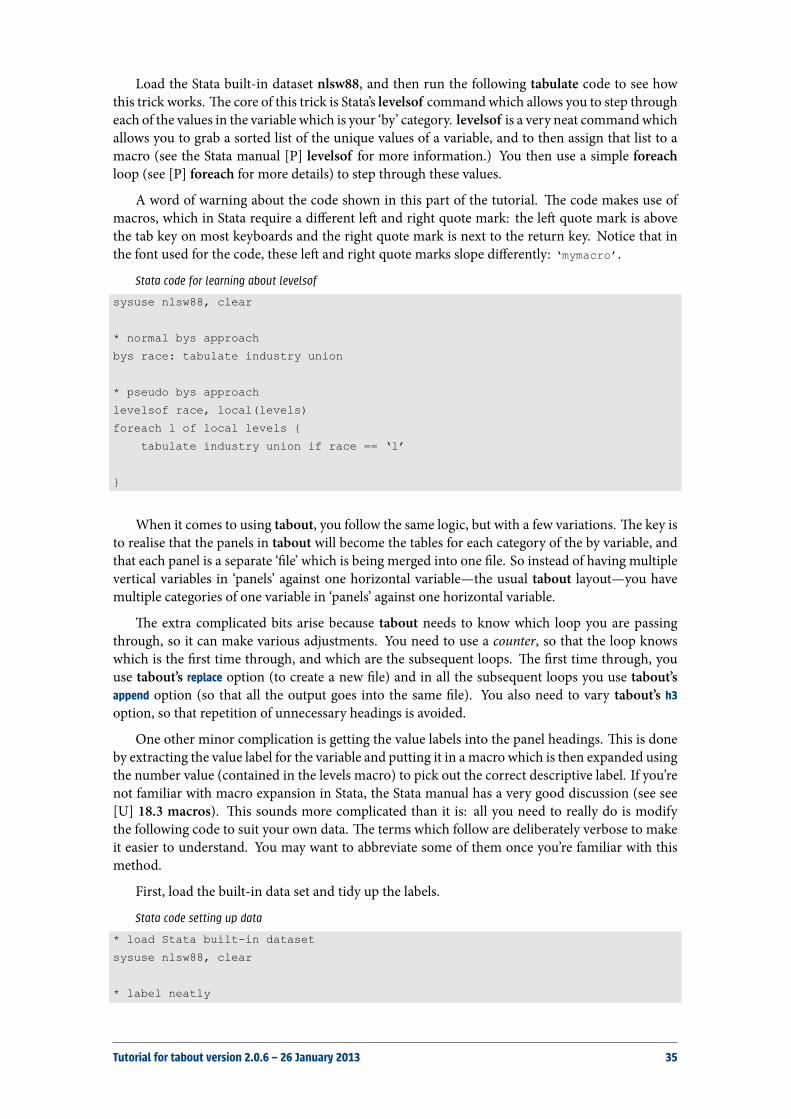
Load the Stata built-in dataset nlsw88, and then run the following tabulate code to see howthis trick works. e core of this trick is Stata’s levelsof command which allows you to step througheach of the values in the variable which is your ‘by’ category. levelsof is a very neat commandwhichallows you to grab a sorted list of the unique values of a variable, and to then assign that list to amacro (see the Stata manual [P] levelsof for more information.) You then use a simple foreachloop (see [P] foreach for more details) to step through these values.
A word of warning about the code shown in this part of the tutorial. e code makes use ofmacros, which in Stata require a different le and right quote mark: the le quote mark is abovethe tab key on most keyboards and the right quote mark is next to the return key. Notice that inthe font used for the code, these le and right quote marks slope differently: ‘mymacro’.
Stata code for learning about levelsof
sysuse nlsw88, clear
* normal bys approach
bys race: tabulate industry union
* pseudo bys approach
levelsof race, local(levels)
foreach l of local levels {
tabulate industry union if race == ‘l’
}
When it comes to using tabout, you follow the same logic, but with a few variations. e key isto realise that the panels in tabout will become the tables for each category of the by variable, andthat each panel is a separate ‘ le’ which is being merged into one le. So instead of having multiplevertical variables in ‘panels’ against one horizontal variable—the usual tabout layout—you havemultiple categories of one variable in ‘panels’ against one horizontal variable.
e extra complicated bits arise because tabout needs to know which loop you are passingthrough, so it can make various adjustments. You need to use a counter, so that the loop knowswhich is the rst time through, and which are the subsequent loops. e rst time through, youuse tabout’s replace option (to create a new le) and in all the subsequent loops you use tabout’sappend option (so that all the output goes into the same le). You also need to vary tabout’s h3option, so that repetition of unnecessary headings is avoided.
One other minor complication is getting the value labels into the panel headings. is is doneby extracting the value label for the variable and putting it in a macro which is then expanded usingthe number value (contained in the levels macro) to pick out the correct descriptive label. If you’renot familiar with macro expansion in Stata, the Stata manual has a very good discussion (see see[U] 18.3 macros). is sounds more complicated than it is: all you need to really do is modifythe following code to suit your own data. e terms which follow are deliberately verbose to makeit easier to understand. You may want to abbreviate some of them once you’re familiar with thismethod.
First, load the built-in data set and tidy up the labels.
Stata code setting up data
* load Stata built-in dataset
sysuse nlsw88, clear
* label neatly
Tutorial for tabout version 2.0.6 – 26 January 2013 35
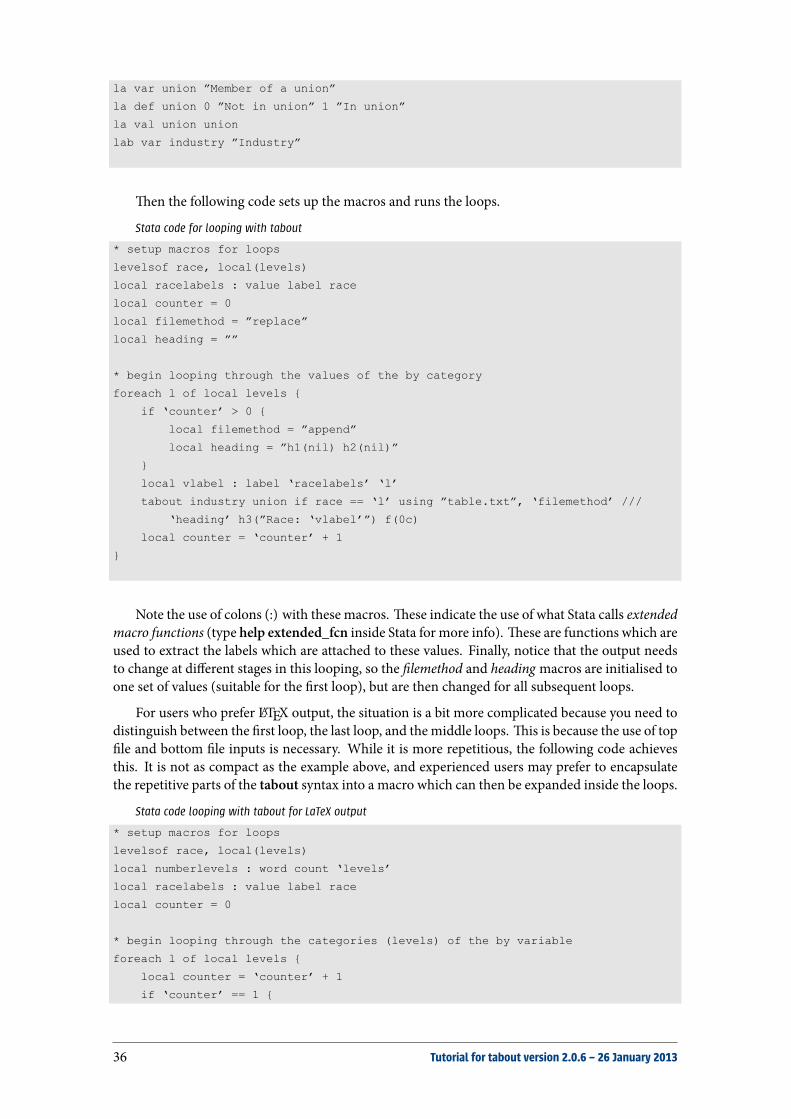
la var union ”Member of a union”
la def union 0 ”Not in union” 1 ”In union”
la val union union
lab var industry ”Industry”
en the following code sets up the macros and runs the loops.
Stata code for looping with tabout
* setup macros for loops
levelsof race, local(levels)
local racelabels : value label race
local counter = 0
local filemethod = ”replace”
local heading = ””
* begin looping through the values of the by category
foreach l of local levels {
if ‘counter’ > 0 {
local filemethod = ”append”
local heading = ”h1(nil) h2(nil)”
}
local vlabel : label ‘racelabels’ ‘l’
tabout industry union if race == ‘l’ using ”table.txt”, ‘filemethod’ ///
‘heading’ h3(”Race: ‘vlabel’”) f(0c)
local counter = ‘counter’ + 1
}
Note the use of colons (:) with these macros. ese indicate the use of what Stata calls extendedmacro functions (type help extended_fcn inside Stata for more info). ese are functions which areused to extract the labels which are attached to these values. Finally, notice that the output needsto change at different stages in this looping, so the lemethod and heading macros are initialised toone set of values (suitable for the rst loop), but are then changed for all subsequent loops.
For users who prefer LATEX output, the situation is a bit more complicated because you need todistinguish between the rst loop, the last loop, and themiddle loops. is is because the use of tople and bottom le inputs is necessary. While it is more repetitious, the following code achieves
this. It is not as compact as the example above, and experienced users may prefer to encapsulatethe repetitive parts of the tabout syntax into a macro which can then be expanded inside the loops.
Stata code looping with tabout for LaTeX output
* setup macros for loops
levelsof race, local(levels)
local numberlevels : word count ‘levels’
local racelabels : value label race
local counter = 0
* begin looping through the categories (levels) of the by variable
foreach l of local levels {
local counter = ‘counter’ + 1
if ‘counter’ == 1 {
36 Tutorial for tabout version 2.0.6 – 26 January 2013
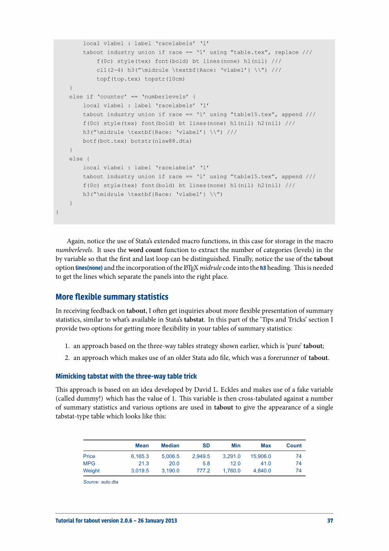
local vlabel : label ‘racelabels’ ‘l’
tabout industry union if race == ‘l’ using ”table.tex”, replace ///
f(0c) style(tex) font(bold) bt lines(none) h1(nil) ///
cl1(2-4) h3(”\midrule \textbf{Race: ‘vlabel’} \\”) ///
topf(top.tex) topstr(10cm)
}
else if ‘counter’ == ‘numberlevels’ {
local vlabel : label ‘racelabels’ ‘l’
tabout industry union if race == ‘l’ using ”table15.tex”, append ///
f(0c) style(tex) font(bold) bt lines(none) h1(nil) h2(nil) ///
h3(”\midrule \textbf{Race: ‘vlabel’} \\”) ///
botf(bot.tex) botstr(nlsw88.dta)
}
else {
local vlabel : label ‘racelabels’ ‘l’
tabout industry union if race == ‘l’ using ”table15.tex”, append ///
f(0c) style(tex) font(bold) bt lines(none) h1(nil) h2(nil) ///
h3(”\midrule \textbf{Race: ‘vlabel’} \\”)
}
}
Again, notice the use of Stata’s extended macro functions, in this case for storage in the macronumberlevels. It uses the word count function to extract the number of categories (levels) in theby variable so that the rst and last loop can be distinguished. Finally, notice the use of the taboutoption lines(none) and the incorporation of the LATEXmidrule code into the h3 heading. is is neededto get the lines which separate the panels into the right place.
More flexible summary statisticsIn receiving feedback on tabout, I oen get inquiries about more exible presentation of summarystatistics, similar to what’s available in Stata’s tabstat. In this part of the ‘Tips and Tricks’ section Iprovide two options for getting more exibility in your tables of summary statistics:
1. an approach based on the three-way tables strategy shown earlier, which is ‘pure’ tabout;2. an approach which makes use of an older Stata ado le, which was a forerunner of tabout.
Mimicking tabstat with the three-way table trick
is approach is based on an idea developed by David L. Eckles and makes use of a fake variable(called dummy!) which has the value of 1. is variable is then cross-tabulated against a numberof summary statistics and various options are used in tabout to give the appearance of a singletabstat-type table which looks like this:
Mean Median SD Min Max Count
Price 6,165.3 5,006.5 2,949.5 3,291.0 15,906.0 74MPG 21.3 20.0 5.8 12.0 41.0 74Weight 3,019.5 3,190.0 777.2 1,760.0 4,840.0 74
Source: auto.dta
Tutorial for tabout version 2.0.6 – 26 January 2013 37
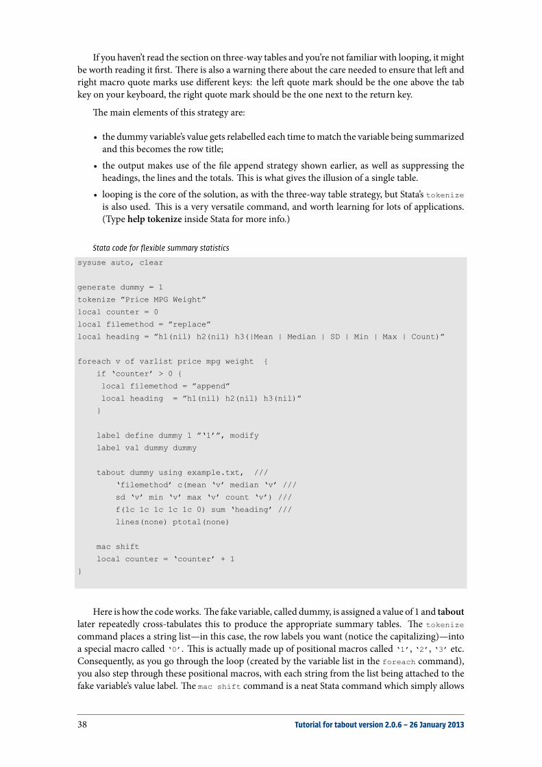
If you haven’t read the section on three-way tables and you’re not familiar with looping, it mightbe worth reading it rst. ere is also a warning there about the care needed to ensure that le andright macro quote marks use different keys: the le quote mark should be the one above the tabkey on your keyboard, the right quote mark should be the one next to the return key.
e main elements of this strategy are:
• the dummy variable’s value gets relabelled each time tomatch the variable being summarizedand this becomes the row title;
• the output makes use of the le append strategy shown earlier, as well as suppressing theheadings, the lines and the totals. is is what gives the illusion of a single table.
• looping is the core of the solution, as with the three-way table strategy, but Stata’s tokenizeis also used. is is a very versatile command, and worth learning for lots of applications.(Type help tokenize inside Stata for more info.)
Stata code for flexible summary statistics
sysuse auto, clear
generate dummy = 1
tokenize ”Price MPG Weight”
local counter = 0
local filemethod = ”replace”
local heading = ”h1(nil) h2(nil) h3(|Mean | Median | SD | Min | Max | Count)”
foreach v of varlist price mpg weight {
if ‘counter’ > 0 {
local filemethod = ”append”
local heading = ”h1(nil) h2(nil) h3(nil)”
}
label define dummy 1 ”‘1’”, modify
label val dummy dummy
tabout dummy using example.txt, ///
‘filemethod’ c(mean ‘v’ median ‘v’ ///
sd ‘v’ min ‘v’ max ‘v’ count ‘v’) ///
f(1c 1c 1c 1c 1c 0) sum ‘heading’ ///
lines(none) ptotal(none)
mac shift
local counter = ‘counter’ + 1
}
Here is how the codeworks. e fake variable, called dummy, is assigned a value of 1 and taboutlater repeatedly cross-tabulates this to produce the appropriate summary tables. e tokenize
command places a string list—in this case, the row labels you want (notice the capitalizing)—intoa special macro called ‘0’. is is actually made up of positional macros called ‘1’, ‘2’, ‘3’ etc.Consequently, as you go through the loop (created by the variable list in the foreach command),you also step through these positional macros, with each string from the list being attached to thefake variable’s value label. e mac shift command is a neat Stata command which simply allows
38 Tutorial for tabout version 2.0.6 – 26 January 2013
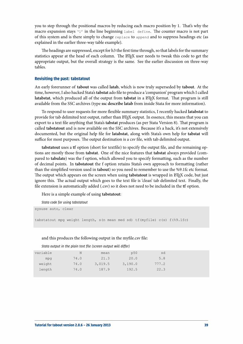
you to step through the positional macros by reducing each macro position by 1. at’s why themacro expansion stays ‘1’ in the line beginning label define. e counter macro is not partof this system and is there simply to change replace to append and to suppress headings etc (asexplained in the earlier three-way table example).
e headings are suppressed, except for h3 the rst time through, so that labels for the summarystatistics appear at the head of each column. e LATEX user needs to tweak this code to get theappropriate output, but the overall strategy is the same. See the earlier discussion on three-waytables.
Revisiting the past: tabstatout
An early forerunner of tabout was called latab, which is now truly superseded by tabout. At thetime, however, I also hacked Stata’s tabstat ado le to produce a ‘companion’ programwhich I calledlatabstat, which produced all of the output from tabstat in a LATEX format. at program is stillavailable from the SSC archives (type ssc describe latab from inside Stata for more information).
To respond to user requests for more exible summary statistics, I recently hacked latabstat toprovide for tab delimited text output, rather than LATEX output. In essence, this means that you canexport to a text le anything that Stata’s tabstat produces (as per Stata Version 8). at program iscalled tabstatout and is now available on the SSC archives. Because it’s a hack, it’s not extensivelydocumented, but the original help le for latabstat, along with Stata’s own help for tabstat willsuffice for most purposes. e output destination is a csv le, with tab delimited output.
tabstatout uses a tf option (short for text le) to specify the output le, and the remaining op-tions are mostly those from tabstat. One of the nice features that tabstat always provided (com-pared to tabulate) was the f option, which allowed you to specify formatting, such as the numberof decimal points. In tabstatout the f option retains Stata’s own approach to formatting (ratherthan the simpli ed version used in tabout) so you need to remember to use the %9.1fc etc format.e output which appears on the screen when using tabstatout is wrapped in LATEX code, but justignore this. e actual output which goes to the text le is ‘clean’ tab delimited text. Finally, thele extension is automatically added (.csv) so it does not need to be included in the tf option.
Here is a simple example of using tabstatout:
Stata code for using tabstatout
sysuse auto, clear
tabstatout mpg weight length, s(n mean med sd) tf(myfile) c(s) f(%9.1fc)
and this produces the following output in the my le.csv le:
Stata output in the plain text file (screen output will differ)
variable N mean p50 sd
mpg 74.0 21.3 20.0 5.8
weight 74.0 3,019.5 3,190.0 777.2
length 74.0 187.9 192.5 22.3
Tutorial for tabout version 2.0.6 – 26 January 2013 39

Yes / no responses in surveysIt is quite common in survey data to nd a battery of questions which all take ‘yes’ or ‘no’ for theiranswer. Tabulating these as a series of twoway tables can be tedious, and produces unnecessaryoutput. Aer all, if 70 per cent answer ‘yes’, then obviously 30 per cent answer ‘no’ (leaving asidethe issue of how you deal with missings and whether you need to allow for residual categories like‘don’t know’).
A useful way to present this data is to recode all the ‘yes’ responses to 100, and the ‘no’ re-sponses to 0. en use tabout’s summary tables to produce tables of means. e cell contents willequate to the percentage of those who answered yes, which is generally the information you wantto present. e advantage of this approach is that the cross-tabulation of this battery of answers byother variables (such as demographics like age, sex, race) ts neatly into one table, with a panel foreach demographic and the columns composed of a series of percentages of those answering yes toeach question.
Usually you would recode into a new variable to preserve the original, but this is optional. Hereis a ctional example to illustrate the syntax:
Stata code for Yes/No example
foreach v of varlist q9a-q9f {
recode ‘v’ (1 = 100) (2 = 0), gen(new_‘v’)
}
tabout sex age race using table.txt, ///
c(mean new_q9a mean new_q9b mean new_q9c mean new_q9d mean new_q9e mean new_q9f) ///
f(1) clab(%) sum
‘File already open …’ messagesUsers may have encountered a message like “File table1.txt is already open inside another applica-tion. Please close it before running tabout.” If so, the problem you’ve hit is an operating system one.It’s caused by le locking, where Stata (rather than tabout) can’t write to a le because it thinks it’sbeing used by another application. Having the le open in Excel is a common cause of this problem.Perhaps you opened it to have a peek, and then resumed working in Stata. is can also happenif you’ve opened the output le in a text editor or word processor. Sometimes, closing the otherapplication solves the problem, sometimes it doesn’t. Sometimes you even need to close Stata andreboot your computer.
You also have the option of directly taking control and forcing Stata to close all open les. ereare two ways of doing this. You can either issue the following command inside Stata:
forvalues i=0(1)50 {
capture mata: fclose(‘i’)
}
or, secondly, you can use a mata function provided by Bill Gould back in 2007 when this problemwas rst raised:
void closeallfiles()
{
real scalar i
for(i=0; i<=50; i++) {
(void) _stata(sprintf(”mata: fclose(%g)”, i), 1)
}
}
40 Tutorial for tabout version 2.0.6 – 26 January 2013
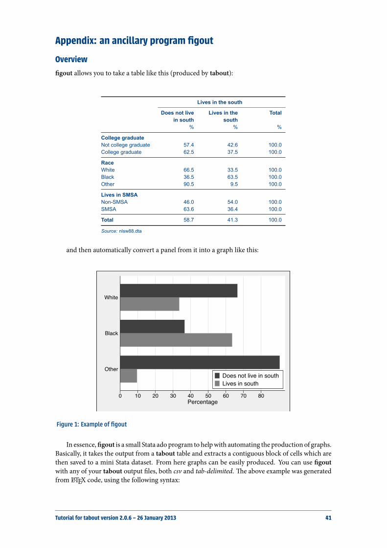
Appendix: an ancillary program figout
Overviewgout allows you to take a table like this (produced by tabout):
Lives in the south
Does not livein south
Lives in thesouth
Total
% % %
College graduateNot college graduate 57.4 42.6 100.0College graduate 62.5 37.5 100.0
RaceWhite 66.5 33.5 100.0Black 36.5 63.5 100.0Other 90.5 9.5 100.0
Lives in SMSANon-SMSA 46.0 54.0 100.0SMSA 63.6 36.4 100.0
Total 58.7 41.3 100.0
Source: nlsw88.dta
and then automatically convert a panel from it into a graph like this:
0 10 20 30 40 50 60 70 80Percentage
Other
Black
White
Does not live in southLives in south
Figure 1: Example of figout
In essence, gout is a small Stata adoprogram tohelpwith automating the production of graphs.Basically, it takes the output from a tabout table and extracts a contiguous block of cells which arethen saved to a mini Stata dataset. From here graphs can be easily produced. You can use goutwith any of your tabout output les, both csv and tab-delimited. e above example was generatedfrom LATEX code, using the following syntax:
Tutorial for tabout version 2.0.6 – 26 January 2013 41

Stata code for tabout and figout
sysuse nlsw88, clear
gen wt = int(uniform()*10)
la var south ”Lives in the south”
la def south 0 ”Does not live in the South” ///
1 ”Lives in the South”
la val south south
la var race ”Race”
la def race 1 ”White” 2 ”Black” 3 ”Other”
la val race race
la var collgrad ”College Graduate”
la def collgrad 0 ”Not college graduate” 1 ”College graduate”
la val collgrad collgrad
la var smsa ”Lives in SMSA”
la def smsa 0 ”Non-SMSA” 1 ”SMSA”
la val smsa smsa
tabout coll race smsa south [iw=wt] using fig_tab.tex, c(row) f(1) ///
style(tex) bt font(bold) topf(top.tex) botf(bot.tex) topstr(10cm) ///
botstr(nlsw88.dta) cl1(2-4) ptot(single)
figout using fig_fig, infile(fig_tab.tex) rep ///
gvars(not_south south) ///
over(race) start(Race) stop(\midrule)
gr hbar not_south south, over(race, sort(order)) ///
ytitle(”Percentage”, size(medium) ) ///
ylab(0(10)80, angle(0) format(%9.0f) ) ///
bar(1,bcolor(gs4)) bar(2,bcolor(gs8)) ///
legend(label( 1 ”Does not live in south”) ///
label(2 ”Lives in south”) ///
pos(4) cols(1) symxsize(3) ring(0) size(medium) ) ///
graphregion(lstyle(solid)) ///
scheme(s2mono) scale(1.1) saving(fig_fig,replace)
gr use fig_fig.gph
grexportpdf using fig_fig
And here is the tabout output which was read by gout to produce the mini dataset:
Output from tabout which will be fed into figout
\begin{center}
\footnotesize
\newcolumntype{Y}{>{\raggedleft\arraybackslash}X}
\begin{tabularx} {10cm} {@{} l Y Y Y Y Y Y Y Y Y Y Y Y Y Y Y Y@{}} \\
\toprule
& \multicolumn{3}{c}{\textbf{Lives in the south}} \\
42 Tutorial for tabout version 2.0.6 – 26 January 2013
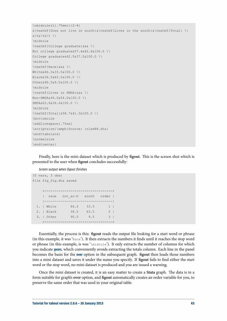
\cmidrule(l{.75em}){2-4}
&\textbf{Does not live in south}&\textbf{Lives in the south}&\textbf{Total} \\
&\%&\%&\% \\
\midrule
\textbf{College graduate}&&& \\
Not college graduate&57.4&42.6&100.0 \\
College graduate&62.5&37.5&100.0 \\
\midrule
\textbf{Race}&&& \\
White&66.5&33.5&100.0 \\
Black&36.5&63.5&100.0 \\
Other&90.5&9.5&100.0 \\
\midrule
\textbf{Lives in SMSA}&&& \\
Non-SMSA&46.0&54.0&100.0 \\
SMSA&63.6&36.4&100.0 \\
\midrule
\textbf{Total}&58.7&41.3&100.0 \\
\bottomrule
\addlinespace[.75ex]
\scriptsize{\emph{Source: }nlsw88.dta}
\end{tabularx}
\normalsize
\end{center}
Finally, here is the mini dataset which is produced by gout. is is the screen shot which ispresented to the user when gout concludes successfully:
Screen output when figout finishes
(5 vars, 3 obs)
file fig_fig.dta saved
+----------------------------------+
| race not_so~h south order |
|----------------------------------|
1. | White 66.5 33.5 1 |
2. | Black 36.5 63.5 2 |
3. | Other 90.5 9.5 3 |
+----------------------------------+
Essentially, the process is this: gout reads the output le looking for a start word or phrase(in this example, it was ‘Race’). It then extracts the numbers it nds until it reaches the stop wordor phrase (in this example, is was ‘\midrule’). It only extracts the number of columns for whichyou indicate gvars, which conveniently avoids extracting the totals column. Each line in the panelbecomes the basis for the over option in the subsequent graph. gout then loads those numbersinto a mini dataset and saves it under the name you specify. If gout fails to nd either the startword or the stop word, no mini dataset is produced and you are issued a warning.
Once the mini dataset is created, it is an easy matter to create a Stata graph. e data is in aform suitable for graph’s over option, and gout automatically creates an order variable for you, topreserve the same order that was used in your original table.
Tutorial for tabout version 2.0.6 – 26 January 2013 43
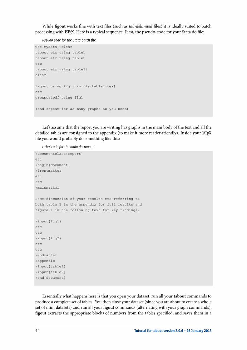
While gout works ne with text les (such as tab-delimited les) it is ideally suited to batchprocessing with LATEX. Here is a typical sequence. First, the pseudo-code for your Stata do le:
Pseudo code for the Stata batch file
use mydata, clear
tabout etc using table1
tabout etc using table2
etc
tabout etc using table99
clear
figout using fig1, infile(table1.tex)
etc
grexportpdf using fig1
(and repeat for as many graphs as you need)
Let’s assume that the report you are writing has graphs in the main body of the text and all thedetailed tables are consigned to the appendix (to make it more reader-friendly). Inside your LATEXle you would probably do something like this:
LaTeX code for the main document
\documentclass{report}
etc
\begin{document}
\frontmatter
etc
etc
\mainmatter
Some discussion of your results etc referring to
both table 1 in the appendix for full results and
figure 1 in the following text for key findings.
\input{fig1}
etc
etc
\input{fig2}
etc
etc
\endmatter
\appendix
\input{table1}
\input{table2}
\end{document}
Essentially what happens here is that you open your dataset, run all your tabout commands toproduce a complete set of tables. You then close your dataset (since you are about to create a wholeset of mini datasets) and run all your gout commands (alternating with your graph commands).gout extracts the appropriate blocks of numbers from the tables speci ed, and saves them in a
44 Tutorial for tabout version 2.0.6 – 26 January 2013

set of mini datasets which becomes the basis for producing graphs. e key points to rememberare: run all your tables rst, because this avoids the need to open and close your main dataset.en close the dataset and run your gout command alternating with your graph commands. eadvantage of a system like this is that you can change your original dataset, perhaps through theaddition of new data or a different weight, rerun all your tables in a batch le and have the graphswhich depend on those tables updated as well. Everything remains in sync.
Note that gout is a Stata Version 8.2 program, so it will workwith the current version of taboutas well as the earlier version.
Syntax
figout using , infile(string) gvars(string) over(string) start(string) stop(string)[replace
]Optionsusing is required, and indicates the lename for the output of the mini Stata dataset. Note that
you do not need to add the dta lename extension.
infile is required and is the nameof the output le produced by tabout, for example, table1.tex.Note that you do need to add the lename extension because you may be using figout
with any number of le types (LATEX, csv, or tab-delimited).
gvars are required and are names you wish to assign to your graph variables, and they need tomatch a contiguous block of cells in your table. ey are basically the categories of the‘horizontal’ variable in your table. (See the example above). Note that this allows you toleave out total columns (since these are rarely used in graphs).
over is required and is the name of the graph variable to be used by the over option in the graphcommand. It is one the panels in your table, and basically matches one of your ‘vertical’variables.
start is required and is a unique word or phrase on the line above the block of cells. It canusually refer to the panel title in a tabout table, unless the title is repeated in anotherpanel.
stop is required and is a unique word or phrase on the line beneath the block of cells. In thecase of LATEX, you can just use \midrule since this generally indicates the end of a panelif you are using the ptotal(single) option.
replace is optional and follows usual Stata convention and prevents you accidentally over-writing an existing Stata dataset with your new mini dataset. If you are con dent thatthere are no other datasets with the same name, you can use the replace option andthis makes it more convenient if you need to develop your figout code using severalattempts.
Tutorial for tabout version 2.0.6 – 26 January 2013 45
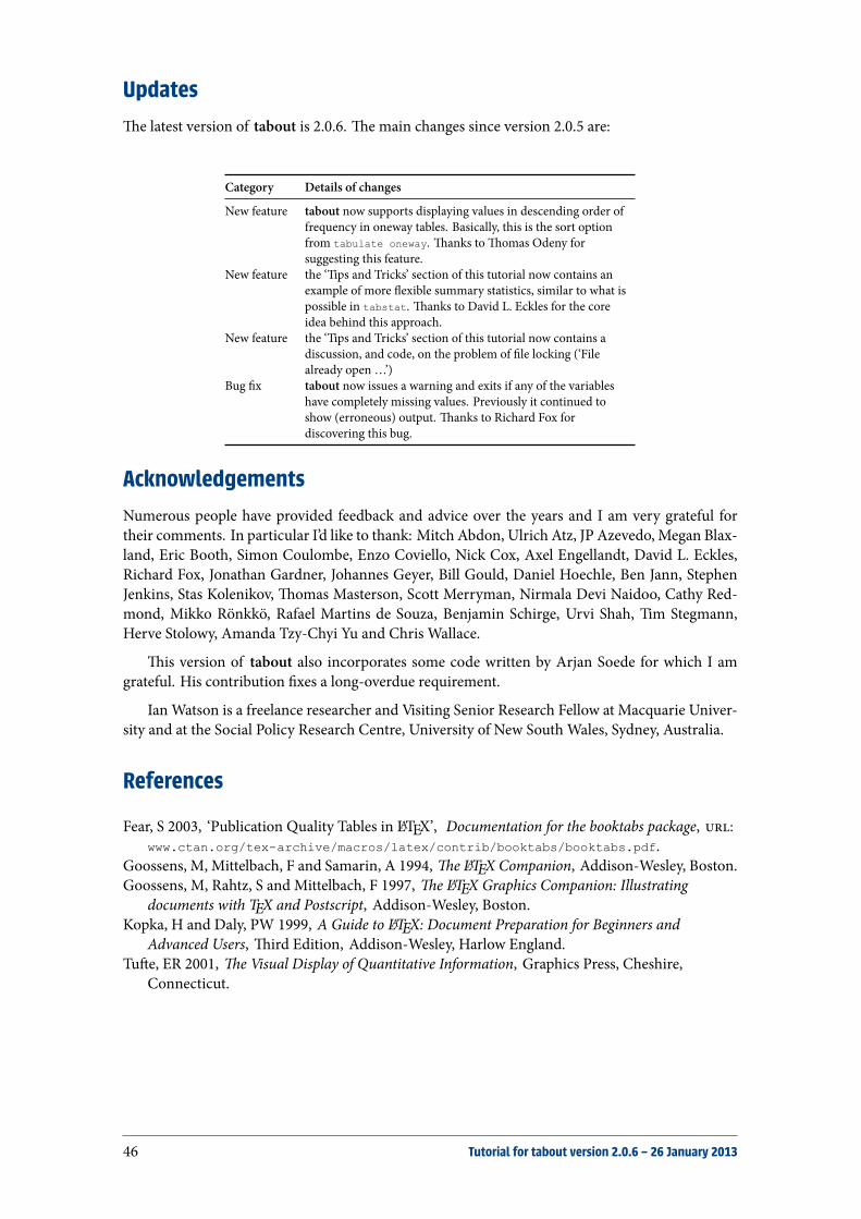
Updatese latest version of tabout is 2.0.6. e main changes since version 2.0.5 are:
Category Details of changes
New feature tabout now supports displaying values in descending order offrequency in oneway tables. Basically, this is the sort optionfrom tabulate oneway. anks to omas Odeny forsuggesting this feature.
New feature the ‘Tips and Tricks’ section of this tutorial now contains anexample of more exible summary statistics, similar to what ispossible in tabstat. anks to David L. Eckles for the coreidea behind this approach.
New feature the ‘Tips and Tricks’ section of this tutorial now contains adiscussion, and code, on the problem of le locking (‘Filealready open …’)
Bug x tabout now issues a warning and exits if any of the variableshave completely missing values. Previously it continued toshow (erroneous) output. anks to Richard Fox fordiscovering this bug.
AcknowledgementsNumerous people have provided feedback and advice over the years and I am very grateful fortheir comments. In particular I’d like to thank: Mitch Abdon, Ulrich Atz, JP Azevedo, Megan Blax-land, Eric Booth, Simon Coulombe, Enzo Coviello, Nick Cox, Axel Engellandt, David L. Eckles,Richard Fox, Jonathan Gardner, Johannes Geyer, Bill Gould, Daniel Hoechle, Ben Jann, StephenJenkins, Stas Kolenikov, omas Masterson, Scott Merryman, Nirmala Devi Naidoo, Cathy Red-mond, Mikko Rönkkö, Rafael Martins de Souza, Benjamin Schirge, Urvi Shah, Tim Stegmann,Herve Stolowy, Amanda Tzy-Chyi Yu and Chris Wallace.
is version of tabout also incorporates some code written by Arjan Soede for which I amgrateful. His contribution xes a long-overdue requirement.
Ian Watson is a freelance researcher and Visiting Senior Research Fellow at Macquarie Univer-sity and at the Social Policy Research Centre, University of New South Wales, Sydney, Australia.
References
Fear, S 2003, ‘Publication Quality Tables in LATEX’, Documentation for the booktabs package, :www.ctan.org/tex-archive/macros/latex/contrib/booktabs/booktabs.pdf.
Goossens, M, Mittelbach, F and Samarin, A 1994, e LATEX Companion, Addison-Wesley, Boston.Goossens, M, Rahtz, S and Mittelbach, F 1997, e LATEX Graphics Companion: Illustrating
documents with TEX and Postscript, Addison-Wesley, Boston.Kopka, H and Daly, PW 1999, A Guide to LATEX: Document Preparation for Beginners and
Advanced Users, ird Edition, Addison-Wesley, Harlow England.Tue, ER 2001, e Visual Display of Quantitative Information, Graphics Press, Cheshire,
Connecticut.
46 Tutorial for tabout version 2.0.6 – 26 January 2013
Related Documents