Advances in Pure Mathematics, 2019, 9, 347-403 http://www.scirp.org/journal/apm ISSN Online: 2160-0384 ISSN Print: 2160-0368 DOI: 10.4236/apm.2019.94017 Apr. 29, 2019 347 Advances in Pure Mathematics Tables of Pure Quintic Fields Daniel C. Mayer Naglergasse 53, Graz, Austria Abstract By making use of our generalization of Barrucand and Cohn’s theory of prin- cipal factorizations in pure cubic fields ( ) 3 D and their Galois closures ( ) 3 3 , D ζ with 3 possible types to pure quintic fields ( ) 5 L D = and their pure metacyclic normal fields ( ) 5 5 , N D ζ = with 13 possible types, we compile an extensive database with arithmetical invariants of the 900 pairwise non-isomorphic fields N having normalized radicands in the range 3 2 10 D ≤ < . Our classification is based on the Galois cohomology of the unit group U N , viewed as a module over the automorphism group ( ) Gal / N K of N over the cyclotomic field ( ) 5 K ζ = , by employing theorems of Hasse and Iwasawa on the Herbrand quotient of the unit norm index ( ) ( ) / : K NK N U N U by the number ( ) / # NK K of primitive ambiguous principal ideals, which can be interpreted as principal factors of the different / NK D . The precise structure of the 5 -vector space of differential principal factors is expressed in terms of norm kernels and central orthogonal idempo- tents. A connection with integral representation theory is established via class number relations by Parry and Walter involving the index of subfield units ( ) 0 : N U U . The statistical distribution of the 13 principal factorization types and their refined splitting into similarity classes with representative proto- types is discussed thoroughly. Keywords Pure Quintic Fields, Pure Metacyclic Fields, Units, Galois Cohomology, Differential Principal Factorization Types, Similarity Classes, Prototypes, Class Group Structure 1. Introduction At the end of his 1975 article on class numbers of pure quintic fields, Parry How to cite this paper: Mayer, D.C. (2019) Tables of Pure Quintic Fields. Ad- vances in Pure Mathematics, 9, 347-403. https://doi.org/10.4236/apm.2019.94017 Received: December 11, 2018 Accepted: April 26, 2019 Published: April 29, 2019 Copyright © 2019 by author(s) and Scientific Research Publishing Inc. This work is licensed under the Creative Commons Attribution International License (CC BY 4.0). http://creativecommons.org/licenses/by/4.0/ Open Access

Welcome message from author
This document is posted to help you gain knowledge. Please leave a comment to let me know what you think about it! Share it to your friends and learn new things together.
Transcript
Advances in Pure Mathematics, 2019, 9, 347-403 http://www.scirp.org/journal/apm
ISSN Online: 2160-0384 ISSN Print: 2160-0368
DOI: 10.4236/apm.2019.94017 Apr. 29, 2019 347 Advances in Pure Mathematics
Tables of Pure Quintic Fields
Daniel C. Mayer
Naglergasse 53, Graz, Austria
Abstract By making use of our generalization of Barrucand and Cohn’s theory of prin-
cipal factorizations in pure cubic fields ( )3 D and their Galois closures
( )33 , Dζ with 3 possible types to pure quintic fields ( )5L D= and
their pure metacyclic normal fields ( )55 ,N Dζ= with 13 possible types,
we compile an extensive database with arithmetical invariants of the 900 pairwise non-isomorphic fields N having normalized radicands in the range
32 10D≤ < . Our classification is based on the Galois cohomology of the unit group UN, viewed as a module over the automorphism group ( )Gal /N K of
N over the cyclotomic field ( )5K ζ= , by employing theorems of Hasse
and Iwasawa on the Herbrand quotient of the unit norm index
( )( )/:K N K NU N U by the number ( )/# N K K of primitive ambiguous
principal ideals, which can be interpreted as principal factors of the different
/N KD . The precise structure of the 5 -vector space of differential principal factors is expressed in terms of norm kernels and central orthogonal idempo-tents. A connection with integral representation theory is established via class number relations by Parry and Walter involving the index of subfield units ( )0:NU U . The statistical distribution of the 13 principal factorization types
and their refined splitting into similarity classes with representative proto-types is discussed thoroughly.
Keywords Pure Quintic Fields, Pure Metacyclic Fields, Units, Galois Cohomology, Differential Principal Factorization Types, Similarity Classes, Prototypes, Class Group Structure
1. Introduction
At the end of his 1975 article on class numbers of pure quintic fields, Parry
How to cite this paper: Mayer, D.C. (2019) Tables of Pure Quintic Fields. Ad-vances in Pure Mathematics, 9, 347-403. https://doi.org/10.4236/apm.2019.94017 Received: December 11, 2018 Accepted: April 26, 2019 Published: April 29, 2019 Copyright © 2019 by author(s) and Scientific Research Publishing Inc. This work is licensed under the Creative Commons Attribution International License (CC BY 4.0). http://creativecommons.org/licenses/by/4.0/
Open Access

D. C. Mayer
DOI: 10.4236/apm.2019.94017 348 Advances in Pure Mathematics
suggested verbatim: In conclusion, the author would like to say that he believes a numerical study of pure quintic fields would be most interesting ([1] p. 484). Of course, it would have been rather difficult to realize Parry’s desire in 1975. But now, 40 years later, we are in the position to use the powerful computer algebra systems PARI/GP [2] and MAGMA [3] [4] [5] for starting an attack against this hard problem. Prepared by [6] [7] [8] [9], this will actually be done in the present paper.
Even in 1991, when we generalized Barrucand and Cohn’s theory [10] [11] of principal factorization types from pure cubic fields ( )3 D to pure quintic fields ( )5L D= and their pure metacyclic normal closures ( )5
5 ,N Dζ= [12], it was still impossible to verify our hypothesis about the distinction between absolute, intermediate and relative differential principal factors (DPF) ([6] (6.3)) and about the values of the unit norm index ( )( )/:K N K NU N U ([6] (1.3)) by actual computations.
All these conjectures have been proven by our most recent numerical investigations. Our classification is based on the Hasse-Iwasawa theorem about the Herbrand quotient of the unit group NU of the Galois closure N of L as a module over the relative group ( )GalG N K= with respect to the cyclotomic subfield ( )5K ζ= . It only involves the unit norm index ( )( )/:K N K NU N U and our 13 types of differential principal factorizations ([6] Thm. 1.3), but not the index of subfield units ( )0:NU U ([6] §5) in Parry’s class number formula ([6] (5.1)).
We begin with a collection of explicit multiplicity formulas in §2 which are required for understanding the subsequent extensive presentation of our computational results in twenty tables of crucial invariants in §3. This information admits the classification of all 900 pure quintic fields with normalized radicands 32 10D≤ < into 13 DPF types and the refined classification into similarity classes with representative prototypes in §4.
We draw the attention to remaining open questions in §3.3, and we collect theoretical consequences of our experimental results in §4.3. The exposition is concluded with a retrospective final §5.
2. Collection of Multiplicity Formulas
For the convenience of the reader, we provide a summary of formulas for calculating invariants of pure quintic fields ( )5L D= with normalized fifth power free radicands 1D > and their associated pure metacyclic normal fields
( )5,N Dζ= with a primitive fifth root of unity 5ζ ζ= . Let f be the class field theoretic conductor of the relatively quintic Kummer
extension N/K over the cyclotomic field ( )K ζ= . It is also called the conductor of the pure quintic field L. The multiplicity ( )m m f= of the conductor f indicates the number of non-isomorphic pure metacyclic fields N sharing the common conductor f, or also, according to ([6] Prop. 2.1), the number of normalized fifth power free radicands 1D > whose fifth roots
( )5L D=

D. C. Mayer
DOI: 10.4236/apm.2019.94017 349 Advances in Pure Mathematics
generate non-isomorphic pure quintic fields L sharing the common conductor f. The cardinality of a set S is denoted #S.
We adapt the general multiplicity formulas in ([13] Thm. 2, p. 104) to the quintic case 5p = . If L is a field of species 1a ([6] (2.6) and Exm. 2.2), i.e.
4 6 4 415 tf q q= ⋅
, then 4tm = where { }: # | 5, |t q q q f= ∈ ≠ . The explicit values of m in dependence on t are given in Table 1.
If L is a field of species 1b ([6] (2.6) and Exm. 2.2), i.e. 4 2 4 415 tf q q= ⋅
, then
4uvm X= ⋅ where ( ){ }: # | 1, 7 mod 25 , |u q q q f= ∈ ≡ ± ± , :v t u= − and
( )( )1: 4 15
jjjX = − − , that is ( ) 1
1 ,0,1,3,13,51,205,4j j
X≥−
=
. The explicit
values of m in dependence on u and v are given in Table 2. If L is a field of species 2 ([6] (2.6) and Exm. 2.2), i.e. 4 0 4 4
15 tf q q= ⋅ , then
14uvm X −= ⋅ where ( ){ }: # | 1, 7 mod 25 , |u q q q f= ∈ ≡ ± ± , :v t u= − and
( )( )1: 4 15
jjjX = − − , that is ( ) 1
1 ,0,1,3,13,51,205,4j j
X≥−
=
. The explicit
values of m in dependence on u and v are given in Table 3.
3. Classification by DPF Types in 20 Numerical Tables 3.1. DPF Types
The following twenty Tables 6-25 establish a complete classification of all 900 pure metacyclic fields ( ),5N Dζ= with normalized radicands in the range
32 10D≤ < . With the aid of PARI/GP [2] and MAGMA [5] we have determined the differential principal factorization type, T, of each field N by means of other invariants , , ,U A I R ([6] Thm. 6.1). After several weeks of CPU time, the date of completion was September 17, 2018.
The possible DPF types are listed in dependence on , , ,U A I R in Table 4, where the symbol × in the column η , resp. ζ , indicates the existence of a unit
NH U∈ , resp. NZ U∈ , such that ( )/N KN Hη = , resp. ( )/N KN Zζ = . The 5-valuation of the unit norm index ( )/:K N K NU N U is abbreviated by U ([6] (1.3), (6.3)]. Here, ( )1 1 5
2η = + denotes the fundamental unit of ( ) 5K Q+ = .
Table 1. Multiplicity of fields of species 1a.
t 0 1 2 3 4 5
m 1 4 16 64 256 1024
Table 2. Multiplicity of fields of species 1b.
u v 0 1 2 3 4 5
0 m 0 1 3 13 51 205
1 0 4 12 52 204 820
2 0 16 48 208 816
3 0 64 192 832
4 0 256 768

D. C. Mayer
DOI: 10.4236/apm.2019.94017 350 Advances in Pure Mathematics
Table 3. Multiplicity of fields of species 2.
u v 0 1 2 3 4 5
0 m 0 0 1 3 13 51
1 1 0 4 12 52 204
2 4 0 16 48 208 816
3 16 0 64 192 832
4 64 0 256 768
Table 4. Differential principal factorization types, T, of pure metacyclic fields N.
T U η ζ A I R
1α 2 − − 1 0 2
2α 2 − − 1 1 1
3α 2 − − 1 2 0
1β 2 − − 2 0 1
2β 2 − − 2 1 0
γ 2 − − 3 0 0
1δ 1 × − 1 0 1
2δ 1 × − 1 1 0
ε 1 × − 2 0 0
1ζ 1 − × 1 0 1
2ζ 1 − × 1 1 0
η 1 − × 2 0 0
ϑ 0 × × 1 0 0
3.2. Justification of the Computational Techniques
The steps of the following classification algorithm are ordered by increasing requirements of CPU time. To avoid unnecessary time consumption, the algorithm stops at early stages already, as soon as the DPF type is determined unambiguously. The illustrating subfield lattice of N is drawn in Figure 1.
Algorithm 3.1 (Classification into 13 DPF types.) Input: a normalized fifth power free radicand 2D ≥ . Step 1: By purely rational methods, without any number field constructions,
the prime factorization of the radicand D (including the counters 2 4, , ; , ,t u v n s s , §4.2) is determined. If D q= ∈ , ( )2 mod 5q ≡ ± , ( )7 mod 25q ≡ ±/ , then N is a Polya field of type ε ; stop. If D q= ∈ , 5q = or ( )7 mod 25q ≡ ± , then N is a Polya field of type ϑ ; stop.
Step 2: The field L of degree 5 is constructed. The primes 1, , Tq q dividing the conductor f of N/K are determined, and their overlying prime ideals
1, , Tq q in L are computed. By means of at most 5T principal ideal tests of

D. C. Mayer
DOI: 10.4236/apm.2019.94017 351 Advances in Pure Mathematics
Figure 1. Lattices of subfields of N and of subgroups of ( )GalG N= .
the elements of / 51
TL ii==⊕ q , the number
( ){ }1 5 15 : # , , | iT vA TT i Liv v
== ∈ ∈∏ q , that is the cardinality of /L , is
determined. If A T= , then N is a Polya field. If 3A = , then N is of type γ ; stop. If 2A = , 2 4 0s s= = , 1v ≥ , then N is of type ε ; stop. If 1A = ,
2 4 0s s= = , then N is of type ϑ ; stop. Step 3: If 2 1s ≥ or 4 1s ≥ , then the field M of degree 10 is constructed. For
the 2-split primes ( )2 41, , 1mod 5s s+ ≡ ± among the primes 1, , Tq q
dividing the conductor f of N/K, the overlying prime ideals
2 4 2 41 1, , , ,s s s sτ τ
+ + in M are computed. By means of at most 2 45s s+ principal ideal tests of the elements of
( ) ( ) ( )2 4
/ 51// ker
i
s sM L iM K K
N+ ++
==⊕
, where ( )1 4
i iτ+=
for
2 41 i s s≤ ≤ + , the number ( ) ( ){ }2 42 42 41 5 15 : # , , | i
i
s s vs sIs s Miv v +++ =
= ∈ ∈∏
, that is the cardinality of ( ) ( )//
/ ker M LM K KN+ + , is determined. If 2I = ,
then N is of type 3α ; stop. If 1I = , 2A = , then N is of type 2β ; stop. Step 4: If 4 1s ≥ , then the field N of degree 20 is constructed. For all 4-split
primes ( )2 2 41, , 1mod 5s s s+ + ≡ + among the primes 1, , Tq q dividing the
conductor f of N/K, the overlying prime ideals 2 3 2 3
2 2 2 2 2 4 2 4 2 4 2 41 1 1 1, , , , , , , ,s s s s s s s s s s s sτ τ τ τ τ τ
+ + + + + + + +L L L L L L L L in N are computed. By means of at most 425 s principal ideal tests of the elements of ( ) ( ) ( ) ( )( )2 4
2/ / 5 51, 2,1/ keri i
s sN K K N M i sN +
= += ⊕⊕
K K , where
( )2 31 4 2 3
1, i iτ τ τ+ + +=
K L and ( )2 31 4 3 2
2, i iτ τ τ+ + +=
K L for 2 2 41s i s s+ ≤ ≤ + , the number
( ) ( ) ( )( ){ }2 4 1, 2,42 2 2 4 2 4 2
21, 1 2, 1 1, 2, 5 1, 2,15 : # , , , , | i i
i i
s s v vsRs s s s s s Ni sv v v v ++ + + + = +
= ∈ ∈∏
K K , that is the cardinality of ( ) ( )/ // kerN K K N MN , is determined. If 2R = , then N is of type 1α ; stop. If 1R = , 1I = , then N is of type 2α ; stop. If 1R = , 2A = , then N is of type 1β ; stop.
Step 5: If the type of the field N is not yet determined uniquely, then 1U = and there remain the following possibilities. If 1v ≥ , then N is of type 1δ , if
1R = , of type 2δ , if 1I = , and of type ε , if 0R I= = . If 0v = , then a
D. C. Mayer
DOI: 10.4236/apm.2019.94017 352 Advances in Pure Mathematics
fundamental system ( )1 9j jE
≤ ≤ of units is constructed for the unit group NU
of the field N of degree 20, and all relative norms of these units with respect to the cyclotomic subfield K are computed. If ( )/ 5
kN K jN E ζ= for some 1 9j≤ ≤ ,
1 4k≤ ≤ , then N is of type 1ζ , if 1R = , of type 2ζ , if 1I = , and of type η , if 0R I= = . Otherwise the conclusions are the same as for 1v ≥ .
Output: the DPF type of the field ( )55 ,N Dζ= and the decision about its
Polya property. Proof. The claims of Step 1 concerning the types ,ε ϑ are proved in items (1)
and (2) of ([6] Thm. 10.1). For Step 2, the formulas (4.1) and (4.2) in ([6] Thm. 4.1) give an 5 -basis of
the space of absolute differential factors, and the formulas (4.3) and (4.4) in ([6] Cor. 4.1) determine bounds for the 5 -dimension A of the space of absolute DPF in the field L of degree 5. The Polya property was characterized in ([6] Thm. 10.5)], the claim concerning type γ follows from ([6] Thm. 6.1), and the claims about the types ,ε ϑ from ([6] Thm. 8.1 and Thm. 6.1).
For Step 3, the formulas (4.5) and (4.6) in ([6] Thm. 4.3) give an 5 -basis of the space of intermediate differential factors, and the formulas (4.7) and (4.8) in ([6] Cor. 4.2) determine bounds for the 5 -dimension I of the space of intermediate DPF in the field M of degree 10. The claims concerning the types
3 2,α β are consequences of ([6] Thm. 6.1), For Step 4, the formulas (4.9) and (4.10) in ([6] Thm. 4.4) give an 5 -basis of
the space of relative differential factors, and the formulas (4.11) and (4.12) in ([6] Cor. 4.3) determine bounds for the 5 -dimension R of the space of relative DPF in the field N of degree 20. The claims concerning the types 1 2 1, ,α α β are consequences of ([6] Thm. 6.1).
Concerning Step 5, the signature of N is ( ) ( )1 2, 0,10r r = , whence the torsion free Dirichlet unit rank of N is given by 1 2 1 9r r r= + − = . The claims about all types are consequences of ([6] Thm. 6.1), including information on the constitution of the norm group ( )/N K NN U .
Remark 3.1 Whereas the execution of Step 1 and 2 in Algorithm 3.1, implemented as a Magma program [5], is a matter of a few seconds on a machine with two Intel XEON 8-core processors and clock frequency 2 GHz, the CPU time for Step 3 lies in the range of several minutes. The time requirement for Step 4 and 5 can reach hours or even days in spite of code optimizations for the calculation of units, in particular the use of the Magma procedures IndependentUnits() and SetOrderUnitsAreFundamental() prior to the call of UnitGroup().
3.3. Open Problems
We conjecture that considerable amounts of CPU time can be saved in our Algorithm 3.1 by computing the logarithmic 5-class numbers ( )5:F FV v h= of the fields { }, ,F L M N∈ , which admit the determination of the logarithmic indices E, resp. E+ , of subfield units in the Parry [1], resp. Kobayashi [14] [15],

D. C. Mayer
DOI: 10.4236/apm.2019.94017 353 Advances in Pure Mathematics
class number relation, according to the formulas
5 4 , 2 2 .N L M LE V V E V V+= + − ⋅ = + − ⋅ (3.1)
However, first there would be required rigorous proofs of the heuristic connections between ,E E+ and the DPF types in Table 5, where
( ) ( ), 1,0E E+ = implies type 2α , ( ) ( ), 2,0E E+ = implies type 3α ,
( ) ( ), 4, 2E E+ = implies type 1δ , but ( ) ( ), 2,1E E+ = admits types 1 1,α δ ,
( ) ( ), 3,1E E+ = admits types 2 1 2, ,α β δ , ( ) ( ), 4,1E E+ = admits types 2 2,β ζ ,
( ) ( ), 5, 2E E+ = admits types 1 1, , ,β ε ζ ϑ , and ( ) ( ), 6, 2E E+ = admits types ,γ η . ( ) ( ), 0,0E E+ = seems to be impossible.
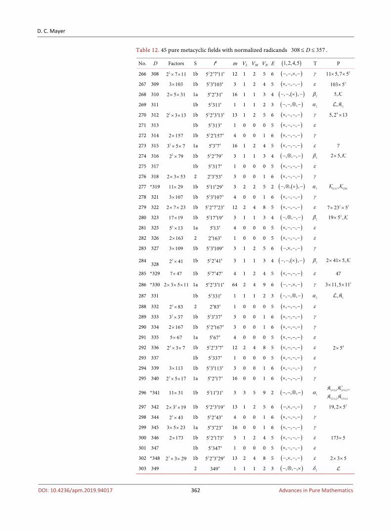
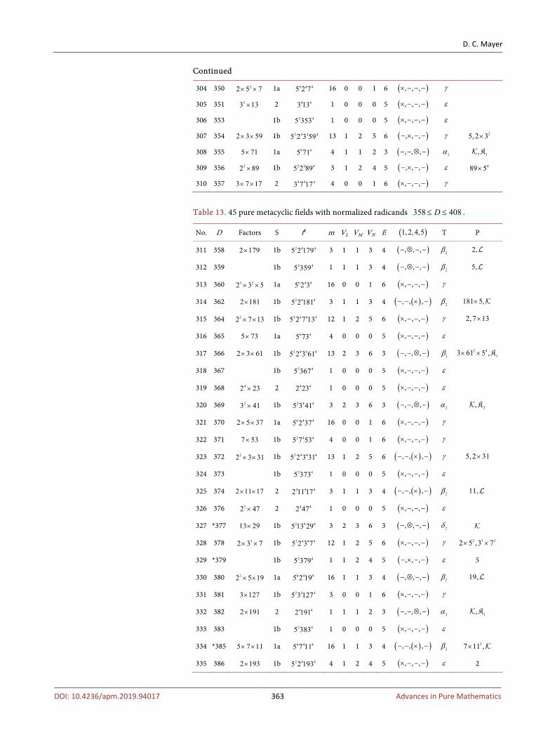
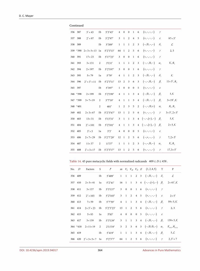
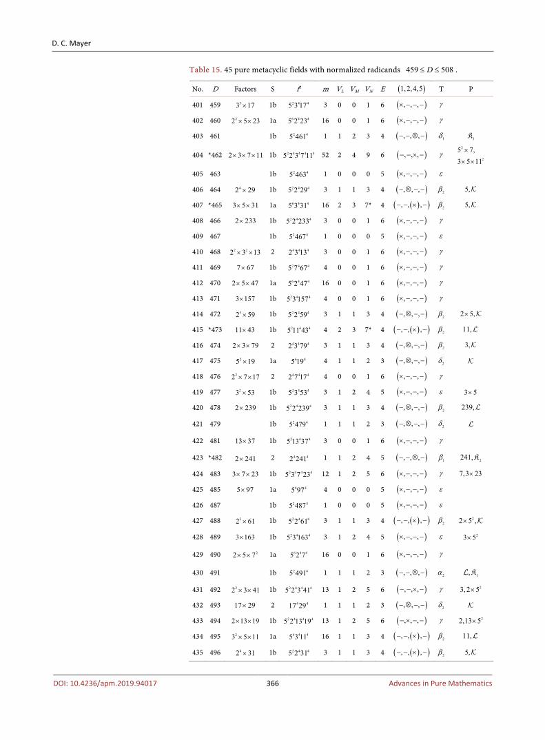
3.4. Conventions and Notation in the Tables
The normalized radicand 11
seesD q q=
of a pure metacyclic field N of degree 20 is minimal among the powers nD , 1 4n≤ ≤ , with corresponding exponents
je reduced modulo 5. The normalization of the radicands D provides a warranty that all fields are pairwise non-isomorphic ([6] Prop. 2.1).
Prime factors are given for composite radicands D only. Dedekind’s species, S, of radicands is refined by distinguishing 5 | D (species 1a) and ( )gcd 5, 1D = (species 1b) among radicands ( )1, 7 mod 25D ≡ ± ±/ (species 1). By the species and factorization of D, the shape of the conductor f is determined. We give the fourth power 4f to avoid fractional exponents. Additionally, the multiplicity m indicates the number of non-isomorphic fields sharing a common conductor f ( § 2). The symbol FV briefly denotes the 5-valuation of the order
( )#ClFh F= of the class group ( )Cl F of a number field F. By E we denote the exponent of the power in the index of subfield units ( )0: 5E
NU U = . Table 5. Logarithmic indices ,E E+ of subfield units for DPF types, T.
T E E+ or E E+
1α 2 1
2α 1 0 3 1
3α 2 0
1β 3 1 5 2
2β 4 1
γ 6 2
1δ 2 1 4 2
2δ 3 1
ε 5 2
1ζ 5 2
2ζ 4 1
η 6 2
ϑ 5 2

D. C. Mayer
DOI: 10.4236/apm.2019.94017 354 Advances in Pure Mathematics
An asterisk denotes the smallest radicand with given Dedekind kind, DPF type and 5-class groups ( )5Cl F , { }, ,F L M N∈ . The latter are usually elementary abelian, except for the cases indicated by an additional asterisk (see §4.4).
Principal factors, P, are listed when their constitution is not a consequence of the other information. According to ([6] Thm. 7.2., item (1)) it suffices to give the rational integer norm of absolute principal factors. For intermediate principal factors, we use the symbols 1: M
τ α−= = with Mα ∈ or
Mλ= with a prime element Mλ ∈ (which implies Mτ τλ= and thus
also 1M
τλ −= ). Here, ( )51M
τ+ = when a prime ( )1mod 5≡ ± divides
the radicand D. For relative principal factors, we use the symbols 2 31 4 2 3
1 1: NAτ τ τ+ + += =K L and 2 31 4 3 2
2 2: NAτ τ τ+ + += =K L with 1 2,A A N∈ . Here, ( )2 3 5
1N
τ τ τ+ + + = L when a prime number ( )1mod 5≡ + divides the
radicand D. (Kernel ideals in [6] §7) The quartet ( )1,2,4,5 indicates conditions which either enforce a reduction
of possible DPF types or enable certain DPF types. The lack of a prime divisor ( )1mod 5≡ ±
together with the existence of a prime divisor ( )7 mod 25q ≡ ±/ and 5q ≠ of D is indicated by a symbol × for the component 1. In these cases, only the two DPF types γ and ε can occur ([6] Thm. 8.1).
A symbol × for the component 2 emphasizes a prime divisor ( )1mod 5≡ −
of D and the possibility of intermediate principal factors in M, like and . A symbol × for the component 4 emphasizes a prime divisor ( )1mod 5≡ +
of D and the possibility of relative principal factors in N, like 1K and 2K . The × symbol is replaced by ⊗ if the facility is used completely, and by (×) if the facility is only used partially.
If D has only prime divisors ( )1, 7 mod 25q ≡ ± ± or 5q = , a symbol × is placed in component 5. In these cases, ζ can occur as a norm ( )/N KN Z of some unit in NZ U∈ . If it actually does, the × is replaced by ⊗ ([6] §8).
4. Statistical Evaluation and Refinements 4.1. Statistics of DPF Types
The complete statistical evaluation of the following twenty Tables 6-25 is given in Table 26. The first ten columns show the absolute frequencies of pure metacyclic fields ( )5,N Dζ= with various DPF types for the ranges 2 100D n≤ < ⋅ with 1 10n≤ ≤ . The eleventh column lists the relative percentages of the five most frequent DPF types for the complete range
32 10D≤ < of normalized radicands. Among our 13 differential principal factorization types, type γ with
3-dimensional absolute principal factorization, 3A = , is clearly dominating with more than one third (36%) of all occurrences in the complete range
32 10D≤ < , followed by type ε with 2-dimensional absolute principal factorization, 2A = , which covers nearly one quarter (23%) of all cases. The third place (nearly 18%) is occupied by type 2β with mixed absolute and intermediate principal factorization, 2A = , 1I = .
D. C. Mayer
DOI: 10.4236/apm.2019.94017 355 Advances in Pure Mathematics
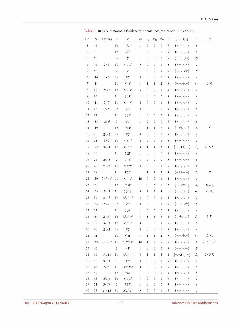
Table 6. 40 pure metacyclic fields with normalized radicands 2 52D≤ ≤ .
No. D Factors S f4 m VL VM VN E ( )1,2,4,5 T P
1 *2 1b 2 45 2 1 0 0 0 5 ( ), , ,× − − − ε
2 3 1b 2 45 3 1 0 0 0 5 ( ), , ,× − − − ε
3 *5 1a 65 1 0 0 0 5 ( ), , ,− − − ⊗ ϑ
4 *6 2 3× 1b 2 4 45 2 3 3 0 0 1 6 ( ), , ,× − − − γ
5 *7 2 47 1 0 0 0 5 ( ), , ,− − − ⊗ ϑ
6 *10 2 5× 1a 6 45 2 4 0 0 0 5 ( ), , ,× − − − ε
7 *11 1b 2 45 11 1 1 1 2 3 ( ), , ,− − ⊗ − 2α 1,K
8 12 22 3× 1b 2 4 45 2 3 3 0 0 1 6 ( ), , ,× − − − γ
9 13 1b 2 45 13 1 0 0 0 5 ( ), , ,× − − − ε
10 *14 2 7× 1b 2 4 45 2 7 4 0 0 1 6 ( ), , ,× − − − γ
11 15 3 5× 1a 6 45 3 4 0 0 0 5 ( ), , ,× − − − ε
12 17 1b 2 45 17 1 0 0 0 5 ( ), , ,× − − − ε
13 *18 22 3× 2 4 42 3 1 0 0 0 5 ( ), , ,× − − − ε
14 *19 1b 2 45 19 1 1 1 2 3 ( ), , ,− ⊗ − − 2δ
15 20 22 5× 1a 6 45 2 4 0 0 0 5 ( ), , ,× − − − ε
16 21 3 7× 1b 2 4 45 3 7 4 0 0 1 6 ( ), , ,× − − − γ
17 *22 2 11× 1b 2 4 45 2 11 3 1 1 3 4 ( )( ), , ,− − × − 2β 2 5,×
18 23 1b 2 45 23 1 0 0 0 5 ( ), , ,× − − − ε
19 26 2 13× 2 4 42 13 1 0 0 0 5 ( ), , ,× − − − ε
20 28 22 7× 1b 2 4 45 2 7 4 0 0 1 6 ( ), , ,× − − − γ
21 29 1b 2 45 29 1 1 1 2 3 ( ), , ,− ⊗ − − 2δ
22 *30 2 3 5× × 1a 6 4 45 2 3 16 0 0 1 6 ( ), , ,× − − − γ
23 *31 1b 2 45 31 1 2 3 5 2 ( ), , ,− − ⊗ − 1α 1 2,K K
24 *33 3 11× 1b 2 4 45 3 11 3 2 2 4 1 ( ), , ,− − ⊗ − 2α 2,K
25 34 2 17× 1b 2 4 45 2 17 3 0 0 1 6 ( ), , ,× − − − γ
26 *35 5 7× 1a 6 45 7 4 0 0 1 6 ( ), , ,− − − ⊗ η
27 37 1b 2 45 37 1 0 0 0 5 ( ), , ,× − − − ε
28 *38 2 19× 1b 2 4 45 2 19 3 1 1 3 4 ( ), , ,− ⊗ − − 2β 5,
29 39 3 13× 1b 2 4 45 3 13 3 0 0 1 6 ( ), , ,× − − − γ
30 40 32 5× 1a 6 45 2 4 0 0 0 5 ( ), , ,× − − − ε
31 41 1b 2 45 41 1 1 1 2 3 ( ), , ,− − ⊗ − 2α 2,K
32 *42 2 3 7× × 1b 2 4 4 45 2 3 7 12 1 2 5 6 ( ), , ,× − − − γ 22 5,3 5× ×
33 43 2 443 1 0 0 0 5 ( ), , ,− − − ⊗ ϑ
34 44 22 11× 1b 2 4 45 2 11 3 1 1 3 4 ( )( ), , ,− − × − 2β 2 5,×
35 45 23 5× 1a 6 45 3 4 0 0 0 5 ( ), , ,× − − − ε
36 46 2 23× 1b 2 4 45 2 23 3 0 0 1 6 ( ), , ,× − − − γ
37 47 1b 2 45 47 1 0 0 0 5 ( ), , ,× − − − ε
38 48 42 3× 1b 2 4 45 2 3 3 0 0 1 6 ( ), , ,× − − − γ
39 51 3 17× 2 4 43 17 1 0 0 0 5 ( ), , ,× − − − ε
40 52 22 13× 1b 2 4 45 2 13 3 0 0 1 6 ( ), , ,× − − − γ
D. C. Mayer
DOI: 10.4236/apm.2019.94017 356 Advances in Pure Mathematics
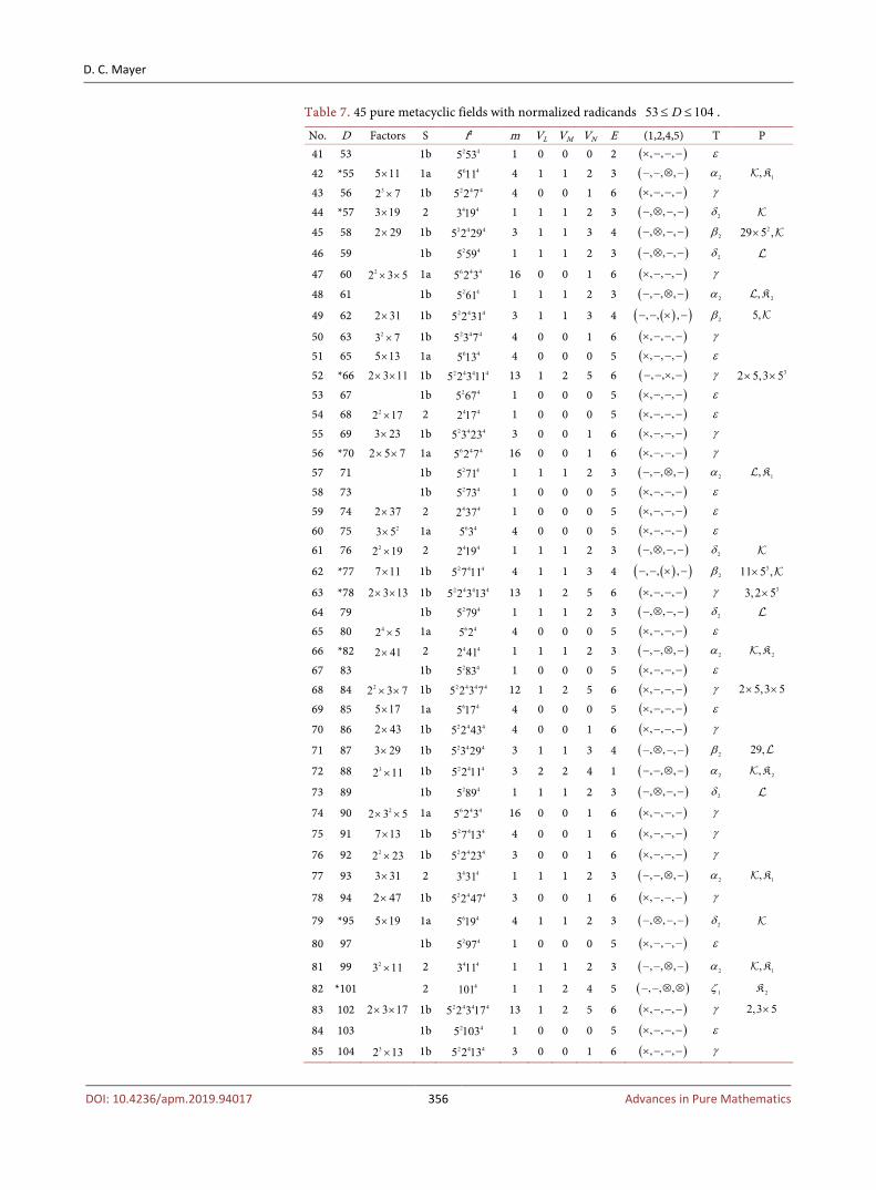
Table 7. 45 pure metacyclic fields with normalized radicands 53 104D≤ ≤ .
No. D Factors S f4 m VL VM VN E (1,2,4,5) T P 41 53 1b 2 45 53 1 0 0 0 2 ( ), , ,× − − − ε
42 *55 5 11× 1a 6 45 11 4 1 1 2 3 ( ), , ,− − ⊗ − 2α 1,K
43 56 32 7× 1b 2 4 45 2 7 4 0 0 1 6 ( ), , ,× − − − γ 44 *57 3 19× 2 4 43 19 1 1 1 2 3 ( ), , ,− ⊗ − − 2δ
45 58 2 29× 1b 2 4 45 2 29 3 1 1 3 4 ( ), , ,− ⊗ − − 2β 229 5 ,×
46 59 1b 2 45 59 1 1 1 2 3 ( ), , ,− ⊗ − − 2δ
47 60 22 3 5× × 1a 6 4 45 2 3 16 0 0 1 6 ( ), , ,× − − − γ
48 61 1b 2 45 61 1 1 1 2 3 ( ), , ,− − ⊗ − 2α 2,K
49 62 2 31× 1b 2 4 45 2 31 3 1 1 3 4 ( )( ), , ,− − × − 2β 5,
50 63 23 7× 1b 2 4 45 3 7 4 0 0 1 6 ( ), , ,× − − − γ 51 65 5 13× 1a 6 45 13 4 0 0 0 5 ( ), , ,× − − − ε
52 *66 2 3 11× × 1b 2 4 4 45 2 3 11 13 1 2 5 6 ( ), , ,− − × − γ 32 5,3 5× × 53 67 1b 2 45 67 1 0 0 0 5 ( ), , ,× − − − ε
54 68 22 17× 2 4 42 17 1 0 0 0 5 ( ), , ,× − − − ε
55 69 3 23× 1b 2 4 45 3 23 3 0 0 1 6 ( ), , ,× − − − γ 56 *70 2 5 7× × 1a 6 4 45 2 7 16 0 0 1 6 ( ), , ,× − − − γ
57 71 1b 2 45 71 1 1 1 2 3 ( ), , ,− − ⊗ − 2α 1,K
58 73 1b 2 45 73 1 0 0 0 5 ( ), , ,× − − − ε
59 74 2 37× 2 4 42 37 1 0 0 0 5 ( ), , ,× − − − ε
60 75 23 5× 1a 6 45 3 4 0 0 0 5 ( ), , ,× − − − ε 61 76 22 19× 2 4 42 19 1 1 1 2 3 ( ), , ,− ⊗ − − 2δ
62 *77 7 11× 1b 2 4 45 7 11 4 1 1 3 4 ( )( ), , ,− − × − 2β 311 5 ,×
63 *78 2 3 13× × 1b 2 4 4 45 2 3 13 13 1 2 5 6 ( ), , ,× − − − γ 33, 2 5× 64 79 1b 2 45 79 1 1 1 2 3 ( ), , ,− ⊗ − − 2δ 65 80 42 5× 1a 6 45 2 4 0 0 0 5 ( ), , ,× − − − ε
66 *82 2 41× 2 4 42 41 1 1 1 2 3 ( ), , ,− − ⊗ − 2α 2,K
67 83 1b 2 45 83 1 0 0 0 5 ( ), , ,× − − − ε
68 84 22 3 7× × 1b 2 4 4 45 2 3 7 12 1 2 5 6 ( ), , ,× − − − γ 2 5,3 5× ×
69 85 5 17× 1a 6 45 17 4 0 0 0 5 ( ), , ,× − − − ε
70 86 2 43× 1b 2 4 45 2 43 4 0 0 1 6 ( ), , ,× − − − γ
71 87 3 29× 1b 2 4 45 3 29 3 1 1 3 4 ( ), , ,− ⊗ − − 2β 29,
72 88 32 11× 1b 2 4 45 2 11 3 2 2 4 1 ( ), , ,− − ⊗ − 2α 2,K
73 89 1b 2 45 89 1 1 1 2 3 ( ), , ,− ⊗ − − 2δ
74 90 22 3 5× × 1a 6 4 45 2 3 16 0 0 1 6 ( ), , ,× − − − γ
75 91 7 13× 1b 2 4 45 7 13 4 0 0 1 6 ( ), , ,× − − − γ
76 92 22 23× 1b 2 4 45 2 23 3 0 0 1 6 ( ), , ,× − − − γ
77 93 3 31× 2 4 43 31 1 1 1 2 3 ( ), , ,− − ⊗ − 2α 1,K
78 94 2 47× 1b 2 4 45 2 47 3 0 0 1 6 ( ), , ,× − − − γ
79 *95 5 19× 1a 6 45 19 4 1 1 2 3 ( ), , ,− ⊗ − − 2δ
80 97 1b 2 45 97 1 0 0 0 5 ( ), , ,× − − − ε
81 99 23 11× 2 4 43 11 1 1 1 2 3 ( ), , ,− − ⊗ − 2α 1,K
82 *101 2 4101 1 1 2 4 5 ( ), , ,− − ⊗ ⊗ 1ζ 2K
83 102 2 3 17× × 1b 2 4 4 45 2 3 17 13 1 2 5 6 ( ), , ,× − − − γ 2,3 5×
84 103 1b 2 45 103 1 0 0 0 5 ( ), , ,× − − − ε
85 104 32 13× 1b 2 4 45 2 13 3 0 0 1 6 ( ), , ,× − − − γ
D. C. Mayer
DOI: 10.4236/apm.2019.94017 357 Advances in Pure Mathematics
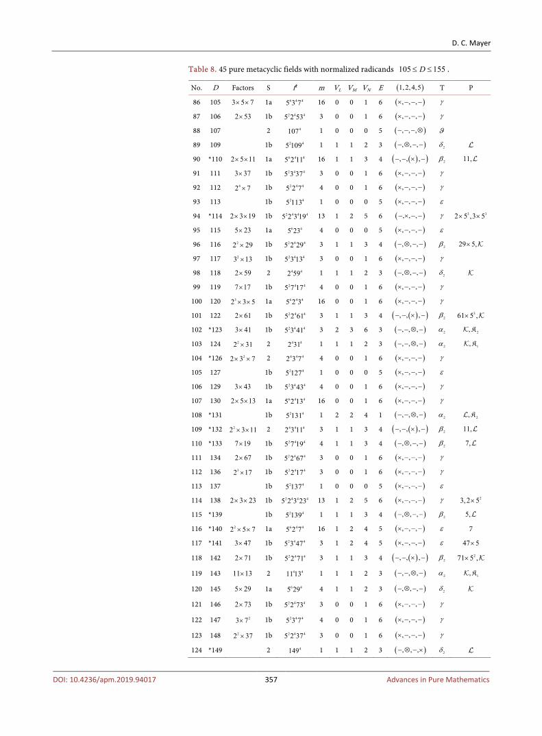
Table 8. 45 pure metacyclic fields with normalized radicands 105 155D≤ ≤ .
No. D Factors S f4 m VL VM VN E ( )1,2,4,5 T P
86 105 3 5 7× × 1a 6 4 45 3 7 16 0 0 1 6 ( ), , ,× − − − γ
87 106 2 53× 1b 2 4 45 2 53 3 0 0 1 6 ( ), , ,× − − − γ
88 107 2 4107 1 0 0 0 5 ( ), , ,− − − ⊗ ϑ
89 109 1b 2 45 109 1 1 1 2 3 ( ), , ,− ⊗ − − 2δ
90 *110 2 5 11× × 1a 6 4 45 2 11 16 1 1 3 4 ( )( ), , ,− − × − 2β 11,
91 111 3 37× 1b 2 4 45 3 37 3 0 0 1 6 ( ), , ,× − − − γ
92 112 42 7× 1b 2 4 45 2 7 4 0 0 1 6 ( ), , ,× − − − γ
93 113 1b 2 45 113 1 0 0 0 5 ( ), , ,× − − − ε
94 *114 2 3 19× × 1b 2 4 4 45 2 3 19 13 1 2 5 6 ( ), , ,− × − − γ 3 32 5 ,3 5× ×
95 115 5 23× 1a 6 45 23 4 0 0 0 5 ( ), , ,× − − − ε
96 116 22 29× 1b 2 4 45 2 29 3 1 1 3 4 ( ), , ,− ⊗ − − 2β 29 5,×
97 117 23 13× 1b 2 4 45 3 13 3 0 0 1 6 ( ), , ,× − − − γ
98 118 2 59× 2 4 42 59 1 1 1 2 3 ( ), , ,− ⊗ − − 2δ
99 119 7 17× 1b 2 4 45 7 17 4 0 0 1 6 ( ), , ,× − − − γ
100 120 32 3 5× × 1a 6 4 45 2 3 16 0 0 1 6 ( ), , ,× − − − γ
101 122 2 61× 1b 2 4 45 2 61 3 1 1 3 4 ( )( ), , ,− − × − 2β 361 5 ,×
102 *123 3 41× 1b 2 4 45 3 41 3 2 3 6 3 ( ), , ,− − ⊗ − 2α 2,K
103 124 22 31× 2 4 42 31 1 1 1 2 3 ( ), , ,− − ⊗ − 2α 1,K
104 *126 22 3 7× × 2 4 4 42 3 7 4 0 0 1 6 ( ), , ,× − − − γ
105 127 1b 2 45 127 1 0 0 0 5 ( ), , ,× − − − ε
106 129 3 43× 1b 2 4 45 3 43 4 0 0 1 6 ( ), , ,× − − − γ
107 130 2 5 13× × 1a 6 4 45 2 13 16 0 0 1 6 ( ), , ,× − − − γ
108 *131 1b 2 45 131 1 2 2 4 1 ( ), , ,− − ⊗ − 2α 2,K
109 *132 22 3 11× × 2 4 4 42 3 11 3 1 1 3 4 ( )( ), , ,− − × − 2β 11,
110 *133 7 19× 1b 2 4 45 7 19 4 1 1 3 4 ( ), , ,− ⊗ − − 2β 7,
111 134 2 67× 1b 2 4 45 2 67 3 0 0 1 6 ( ), , ,× − − − γ
112 136 32 17× 1b 2 4 45 2 17 3 0 0 1 6 ( ), , ,× − − − γ
113 137 1b 2 45 137 1 0 0 0 5 ( ), , ,× − − − ε
114 138 2 3 23× × 1b 2 4 4 45 2 3 23 13 1 2 5 6 ( ), , ,× − − − γ 23, 2 5×
115 *139 1b 2 45 139 1 1 1 3 4 ( ), , ,− ⊗ − − 2β 5,
116 *140 22 5 7× × 1a 6 4 45 2 7 16 1 2 4 5 ( ), , ,× − − − ε 7
117 *141 3 47× 1b 2 4 45 3 47 3 1 2 4 5 ( ), , ,× − − − ε 47 5×
118 142 2 71× 1b 2 4 45 2 71 3 1 1 3 4 ( )( ), , ,− − × − 2β 271 5 ,×
119 143 11 13× 2 4 411 13 1 1 1 2 3 ( ), , ,− − ⊗ − 2α 1,K
120 145 5 29× 1a 6 45 29 4 1 1 2 3 ( ), , ,− ⊗ − − 2δ
121 146 2 73× 1b 2 4 45 2 73 3 0 0 1 6 ( ), , ,× − − − γ
122 147 23 7× 1b 2 4 45 3 7 4 0 0 1 6 ( ), , ,× − − − γ
123 148 22 37× 1b 2 4 45 2 37 3 0 0 1 6 ( ), , ,× − − − γ
124 *149 2 4149 1 1 1 2 3 ( ), , ,− ⊗ − × 2δ
D. C. Mayer
DOI: 10.4236/apm.2019.94017 358 Advances in Pure Mathematics
Continued
125 150 22 3 5× × 1a 6 4 45 2 3 16 0 0 1 6 ( ), , ,× − − − γ
126 *151 2 4151 1 1 1 2 3 ( ), , ,− − ⊗ × 2α 1,K
127 152 32 19× 1b 2 4 45 2 19 3 1 1 3 4 ( ), , ,− ⊗ − − 2β 219 5 ,×
128 153 23 17× 1b 2 4 45 3 17 3 0 0 1 6 ( ), , ,× − − − γ
129 *154 2 7 11× × 1b 2 4 4 45 2 7 11 12 2 3 7 4 ( )( ), , ,− − × − 2β 22 11 ,×
130 *155 5 31× 1a 6 45 31 4 2 3 5 2 ( ), , ,− − ⊗ − 1α 1 2,K K
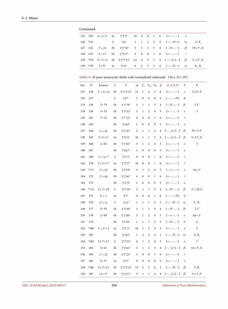
Table 9. 45 pure metacyclic fields with normalized radicands 156 207D≤ ≤ .
No. D Factors S f4 m VL VM VN E ( )1,2,4,5 T P
131 156 22 3 13× × 1b 2 4 4 45 2 3 13 13 1 2 5 6 ( ), , ,× − − − γ 23,13 5×
132 157 2 4157 1 0 0 0 5 ( ), , ,− − − ⊗ ϑ
133 158 2 79× 1b 2 4 45 2 79 3 1 1 3 4 ( ), , ,− ⊗ − − 2β 5,
134 159 3 53× 1b 2 4 45 3 53 3 1 2 4 5 ( ), , ,× − − − ε 5
135 161 7 23× 1b 2 4 45 7 23 4 0 0 1 6 ( ), , ,× − − − γ
136 163 1b 2 45 163 1 0 0 0 5 ( ), , ,× − − − ε
137 164 22 41× 1b 2 4 45 2 41 3 1 1 3 4 ( )( ), , ,− − × − 2β 41 5,×
138 165 3 5 11× × 1a 6 4 45 3 11 16 1 1 3 4 ( )( ), , ,− − × − 2β 25 11 ,×
139 166 2 83× 1b 2 4 45 2 83 3 1 2 4 5 ( ), , ,× − − − ε 5
140 167 1b 2 45 167 1 0 0 0 5 ( ), , ,× − − − ε
141 168 32 3 7× × 2 4 4 42 3 7 4 0 0 1 6 ( ), , ,× − − − γ
142 170 2 5 17× × 1a 6 4 45 2 17 16 0 0 1 6 ( ), , ,× − − − γ
143 *171 23 19× 1b 2 4 45 3 19 3 1 2 4 5 ( ), , ,− × − − ε 219 5×
144 172 22 43× 1b 2 4 45 2 43 4 0 0 1 6 ( ), , ,× − − − γ
145 173 1b 2 45 173 1 0 0 0 5 ( ), , ,× − − − ε
146 *174 2 3 29× × 2 4 4 42 3 29 3 1 1 3 4 ( ), , ,− ⊗ − − 2β 23 29,×
147 175 25 7× 1a 6 45 7 4 0 0 1 6 ( ), , ,− − − ⊗ η
148 176 42 11× 2 4 42 11 1 1 1 2 3 ( ), , ,− − ⊗ − 2α 2, K
149 177 3 59× 1b 2 4 45 3 59 3 1 1 3 4 ( ), , ,− ⊗ − − 2β 3,
150 178 2 89× 1b 2 4 45 2 89 3 1 2 4 5 ( ), , ,− × − − ε 289 5×
151 179 1b 2 45 179 1 1 1 2 3 ( ), , ,− ⊗ − − 2δ
152 *180 2 22 3 5× × 1a 6 4 45 2 3 16 1 2 4 5 ( ), , ,× − − − ε 3
153 181 1b 2 45 181 1 2 2 4 1 ( ), , ,− − ⊗ − 2α 2, K
154 *182 2 7 13× × 2 4 4 42 7 13 4 1 2 4 5 ( ), , ,× − − − ε 7
155 183 3 61× 1b 2 4 45 3 61 3 1 1 3 4 ( )( ), , ,− − × − 2β 361 5 ,×
156 184 32 23× 1b 2 4 45 2 23 3 0 0 1 6 ( ), , ,× − − − γ
157 185 5 37× 1a 6 45 37 4 0 0 0 5 ( ), , ,× − − − ε
158 *186 2 3 31× × 1b 2 4 4 45 2 3 31 13 2 3 6 3 ( ), , ,− − ⊗ − 1β 25,K
159 187 11 17× 1b 2 4 45 11 17 3 1 1 3 4 ( )( ), , ,− − × − 2β 11 5,×
D. C. Mayer
DOI: 10.4236/apm.2019.94017 359 Advances in Pure Mathematics
Continued
160 188 22 47× 1b 2 4 45 2 47 3 0 0 1 6 ( ), , ,× − − − γ
161 *190 2 5 19× × 1a 6 4 45 2 19 16 1 1 3 4 ( ), , ,− ⊗ − − 2β 5,
162 *191 1b 2 45 191 1 1 2 4 5 ( ), , ,− − ⊗ − 1β 15,K
163 193 2 4193 1 0 0 0 5 ( ), , ,− − − ⊗ ϑ
164 194 2 97× 1b 2 4 45 2 97 3 1 2 4 5 ( ), , ,× − − − ε 297 5×
165 195 3 5 13× × 1a 6 4 45 3 13 16 0 0 1 6 ( ), , ,× − − − γ
166 197 1b 2 45 197 1 0 0 0 5 ( ), , ,× − − − ε
167 198 22 3 11× × 1b 2 4 4 45 2 3 11 13 1 2 5 6 ( ), , ,− − × − γ 3 33 5 ,11 5× ×
168 199 2 4199 1 1 1 2 3 ( ), , ,− ⊗ − × 2δ
169 201 3 67× 2 4 43 67 1 0 0 0 5 ( ), , ,× − − − ε
170 *202 2 101× 1b 2 4 45 2 101 4 1 1 3 4 ( )( ), , ,− − × − 2β 2 5,×
171 *203 7 29× 1b 2 4 45 7 29 4 1 2 4 5 ( ), , ,− × − − ε 29 5×
172 204 22 3 17× × 1b 2 4 4 45 2 3 17 13 1 2 5 6 ( ), , ,× − − − γ 4 33 5 ,17 5× ×
173 205 5 41× 1a 6 45 41 4 1 1 2 3 ( ), , ,− − ⊗ − 2α 2, K
174 206 2 103× 1b 2 4 45 2 103 3 1 2 4 5 ( ), , ,× − − − ε 22 5×
175 207 23 23× 2 4 43 23 1 0 0 0 5 ( ), , ,× − − − ε
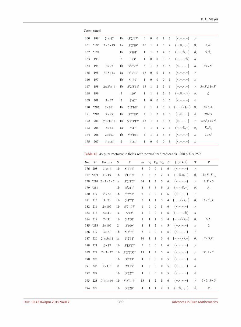
Table 10. 45 pure metacyclic fields with normalized radicands 208 259D≤ ≤ .
No. D Factors S f4 m VL VM VN E ( )1,2,4,5 T P
176 208 42 13× 1b 2 4 45 2 13 3 0 0 1 6 ( ), , ,× − − − γ
177 *209 11 19× 1b 2 4 45 11 19 3 2 3 7 4 ( ), , ,− ⊗ × − 2β 2(19)11 5 ,×
178 *210 2 3 5 7× × × 1a 6 4 4 45 2 3 7 64 1 2 5 6 ( ), , ,× − − − γ 27,3 5×
179 *211 1b 2 45 211 1 3 5 9 2 ( ), , ,− − ⊗ − 1δ 2K
180 212 22 53× 1b 2 4 45 2 53 3 0 0 1 6 ( ), , ,× − − − γ
181 213 3 71× 1b 2 4 45 3 71 3 1 1 3 4 ( )( ), , ,− − × − 2β 33 5 ,×
182 214 2 107× 1b 2 4 45 2 107 4 0 0 1 6 ( ), , ,× − − − γ
183 215 5 43× 1a 6 45 43 4 0 0 1 6 ( ), , ,− − − ⊗ η
184 217 7 31× 1b 2 4 45 7 31 4 1 1 3 4 ( )( ), , ,− − × − 2β 5,
185 *218 2 109× 2 4 42 109 1 1 2 4 5 ( ), , ,− × − − ε 2
186 219 3 73× 1b 2 4 45 3 73 3 0 0 1 6 ( ), , ,× − − − γ
187 220 22 5 11× × 1a 6 4 45 2 11 16 1 1 3 4 ( )( ), , ,− − × − 2β 2 5,×
188 221 13 17× 1b 2 4 45 13 17 3 0 0 1 6 ( ), , ,× − − − γ
189 222 2 3 37× × 1b 2 4 4 45 2 3 37 13 1 2 5 6 ( ), , ,× − − − γ 237,2 5×
190 223 1b 2 45 223 1 0 0 0 5 ( ), , ,× − − − ε
191 226 2 113× 2 4 42 113 1 0 0 0 5 ( ), , ,× − − − ε
192 227 1b 2 45 227 1 0 0 0 5 ( ), , ,× − − − ε
193 228 22 3 19× × 1b 2 4 4 45 2 3 19 13 1 2 5 6 ( ), , ,− × − − γ 3 5,19 5× ×
194 229 1b 2 45 229 1 1 1 2 3 ( ), , ,− ⊗ − − 2δ

D. C. Mayer
DOI: 10.4236/apm.2019.94017 360 Advances in Pure Mathematics
Continued
195 230 2 5 23× × 1a 6 4 45 2 23 16 0 0 1 6 ( ), , ,× − − − γ
196 *231 3 7 11× × 1b 2 4 4 45 3 7 11 12 1 2 2 6 ( ), , ,− − × − γ 211,7 5×
197 232 32 29× 2 4 42 29 1 1 1 2 3 ( ), , ,− ⊗ − − 2δ
198 233 1b 2 45 233 1 0 0 0 5 ( ), , ,× − − − ε
199 234 22 3 13× × 1b 2 4 4 45 2 3 13 13 1 2 5 6 ( ), , ,× − − − γ 3,2 5×
200 235 5 47× 1a 6 45 47 4 0 0 0 5 ( ), , ,× − − − ε
201 236 22 59× 1b 2 4 45 2 59 3 1 1 3 4 ( ), , ,− ⊗ − − 2β 22 5 ,×
202 237 3 79× 1b 2 4 45 3 79 3 1 1 3 4 ( ), , ,− ⊗ − − 2β 3 5,×
203 238 2 7 17× × 1b 2 4 4 45 2 7 17 12 1 2 5 6 ( ), , ,× − − − γ 45, 2 7×
204 239 1b 2 45 239 1 1 1 2 3 ( ), , ,− ⊗ − − 2δ
205 240 42 3 5× × 1a 6 4 45 2 3 16 1 2 4 5 ( ), , ,× − − − ε 3
206 241 1b 2 45 241 1 1 1 2 3 ( ), , ,− − ⊗ − 2α 2, K
207 244 22 61× 1b 2 4 45 2 61 3 2 2 4 1 ( ), , ,− − ⊗ − 2α 1, K
208 245 25 7× 1a 6 45 7 4 0 0 1 6 ( ), , ,− − − ⊗ η
209 246 2 3 41× × 1b 2 4 4 45 2 3 41 13 1 2 5 6 ( ), , ,− − × − γ 23, 2 5⋅
210 *247 13 19× 1b 2 4 45 13 19 3 1 2 5 6 ( ), , ,− × − − γ
211 248 32 31× 1b 2 4 45 2 31 3 1 1 3 4 ( )( ), , ,− − × − 2β 5,
212 249 3 83× 2 4 43 83 1 0 0 0 5 ( ), , ,× − − − ε
213 251 2 4251 1 1 1 2 3 ( ), , ,− − ⊗ × 2α 2, K
214 252 2 22 3 7× × 1b 2 4 4 45 2 3 7 12 1 2 5 6 ( ), , ,× − − − γ 3,2 5×
215 *253 11 23× 1b 2 4 45 11 23 3 1 2 4 5 ( ), , ,− − ⊗ − 1β 111,K
216 254 2 127× 1b 2 4 45 2 127 3 0 0 1 6 ( ), , ,× − − − γ
217 255 3 5 17× × 1a 6 4 45 3 17 16 0 0 1 6 ( ), , ,× − − − γ
218 257 2 4257 1 0 0 0 5 ( ), , ,− − − ⊗ ϑ
219 258 2 3 43× × 1b 2 4 4 45 2 3 43 12 1 2 5 6 ( ), , ,× − − − γ 2,3 5×
220 *259 7 37× 1b 2 4 45 7 37 4 1 2 5* 6 ( ), , ,× − − − γ
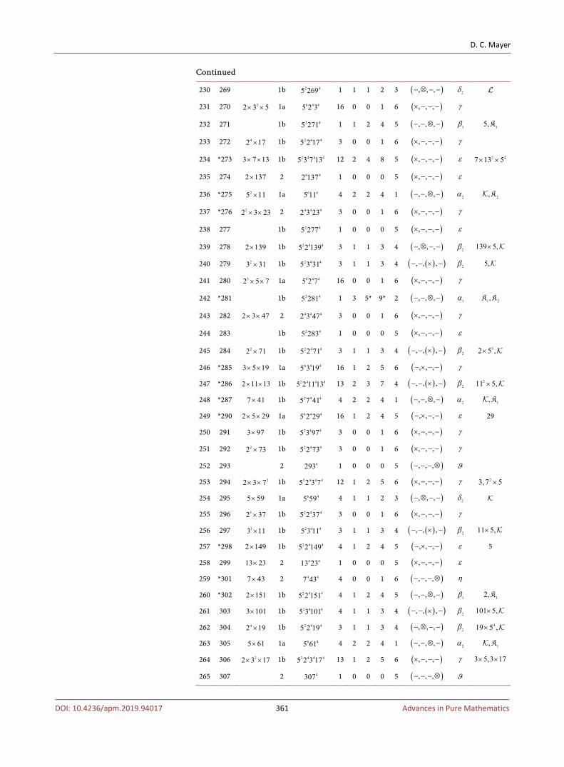
Table 11. 45 pure metacyclic fields with normalized radicands 260 307D≤ ≤ .
No. D Factors S f4 m VL VM VN E ( )1,2,4,5 T P
221 260 22 5 13× × 1a 6 4 45 2 13 16 0 0 1 6 ( ), , ,× − − − γ
222 261 23 29× 1b 2 4 45 3 29 3 1 1 3 4 ( ), , ,− ⊗ − − 2β 29,
223 262 2 131× 1b 2 4 45 2 131 3 1 1 3 4 ( )( ), , ,− − × − 2β 131 5,×
224 263 1b 2 45 263 1 0 0 0 5 ( ), , ,× − − − ε
225 264 32 3 11× × 1b 2 4 4 45 2 3 11 13 1 2 5 6 ( ), , ,− − × − γ 2 5,2 11× ×
226 265 5 53× 1a 6 45 53 4 0 0 0 5 ( ), , ,× − − − ε
227 *266 2 7 19× × 1b 2 4 4 45 2 7 19 12 1 2 5 6 ( ), , ,− × − − γ 35, 2 7×
228 267 3 89× 1b 2 4 45 3 89 3 1 1 3 4 ( ), , ,− ⊗ − − 2β 289 5 ,×
229 268 22 67× 2 4 42 67 1 0 0 0 5 ( ), , ,× − − − ε
D. C. Mayer
DOI: 10.4236/apm.2019.94017 361 Advances in Pure Mathematics
Continued
230 269 1b 2 45 269 1 1 1 2 3 ( ), , ,− ⊗ − − 2δ
231 270 32 3 5× × 1a 6 4 45 2 3 16 0 0 1 6 ( ), , ,× − − − γ
232 271 1b 2 45 271 1 1 2 4 5 ( ), , ,− − ⊗ − 1β 15,K
233 272 42 17× 1b 2 4 45 2 17 3 0 0 1 6 ( ), , ,× − − − γ
234 *273 3 7 13× × 1b 2 4 4 45 3 7 13 12 2 4 8 5 ( ), , ,× − − − ε 2 47 13 5× ×
235 274 2 137× 2 4 42 137 1 0 0 0 5 ( ), , ,× − − − ε
236 *275 25 11× 1a 6 45 11 4 2 2 4 1 ( ), , ,− − ⊗ − 2α 2, K
237 *276 22 3 23× × 2 4 4 42 3 23 3 0 0 1 6 ( ), , ,× − − − γ
238 277 1b 2 45 277 1 0 0 0 5 ( ), , ,× − − − ε
239 278 2 139× 1b 2 4 45 2 139 3 1 1 3 4 ( ), , ,− ⊗ − − 2β 139 5,×
240 279 23 31× 1b 2 4 45 3 31 3 1 1 3 4 ( )( ), , ,− − × − 2β 5,
241 280 32 5 7× × 1a 6 4 45 2 7 16 0 0 1 6 ( ), , ,× − − − γ
242 *281 1b 2 45 281 1 3 5* 9* 2 ( ), , ,− − ⊗ − 1α 1 2,K K
243 282 2 3 47× × 2 4 4 42 3 47 3 0 0 1 6 ( ), , ,× − − − γ
244 283 1b 2 45 283 1 0 0 0 5 ( ), , ,× − − − ε
245 284 22 71× 1b 2 4 45 2 71 3 1 1 3 4 ( )( ), , ,− − × − 2β 32 5 ,×
246 *285 3 5 19× × 1a 6 4 45 3 19 16 1 2 5 6 ( ), , ,− × − − γ
247 *286 2 11 13× × 1b 2 4 4 45 2 11 13 13 2 3 7 4 ( )( ), , ,− − × − 2β 211 5,×
248 *287 7 41× 1b 2 4 45 7 41 4 2 2 4 1 ( ), , ,− − ⊗ − 2α 1, K
249 *290 2 5 29× × 1a 6 4 45 2 29 16 1 2 4 5 ( ), , ,− × − − ε 29
250 291 3 97× 1b 2 4 45 3 97 3 0 0 1 6 ( ), , ,× − − − γ
251 292 22 73× 1b 2 4 45 2 73 3 0 0 1 6 ( ), , ,× − − − γ
252 293 2 4293 1 0 0 0 5 ( ), , ,− − − ⊗ ϑ
253 294 22 3 7× × 1b 2 4 4 45 2 3 7 12 1 2 5 6 ( ), , ,× − − − γ 23,7 5×
254 295 5 59× 1a 6 45 59 4 1 1 2 3 ( ), , ,− ⊗ − − 2δ
255 296 32 37× 1b 2 4 45 2 37 3 0 0 1 6 ( ), , ,× − − − γ
256 297 33 11× 1b 2 4 45 3 11 3 1 1 3 4 ( )( ), , ,− − × − 2β 11 5,×
257 *298 2 149× 1b 2 4 45 2 149 4 1 2 4 5 ( ), , ,− × − − ε 5
258 299 13 23× 2 4 413 23 1 0 0 0 5 ( ), , ,× − − − ε
259 *301 7 43× 2 4 47 43 4 0 0 1 6 ( ), , ,− − − ⊗ η
260 *302 2 151× 1b 2 4 45 2 151 4 1 2 4 5 ( ), , ,− − ⊗ − 1β 12,K
261 303 3 101× 1b 2 4 45 3 101 4 1 1 3 4 ( )( ), , ,− − × − 2β 101 5,×
262 304 42 19× 1b 2 4 45 2 19 3 1 1 3 4 ( ), , ,− ⊗ − − 2β 419 5 ,×
263 305 5 61× 1a 6 45 61 4 2 2 4 1 ( ), , ,− − ⊗ − 2α 1, K
264 306 22 3 17× × 1b 2 4 4 45 2 3 17 13 1 2 5 6 ( ), , ,× − − − γ 3 5,3 17× ×
265 307 2 4307 1 0 0 0 5 ( ), , ,− − − ⊗ ϑ
D. C. Mayer
DOI: 10.4236/apm.2019.94017 362 Advances in Pure Mathematics
Table 12. 45 pure metacyclic fields with normalized radicands 308 357D≤ ≤ .
No. D Factors S f4 m VL VM VN E ( )1,2,4,5 T P
266 308 22 7 11× × 1b 2 4 4 45 2 7 11 12 1 2 5 6 ( ), , ,− − × − γ 211 5,7 5× ×
267 309 3 103× 1b 2 4 45 3 103 3 1 2 4 5 ( ), , ,× − − − ε 2103 5×
268 310 2 5 31× × 1a 6 4 45 2 31 16 1 1 3 4 ( )( ), , ,− − × − 2β 5,
269 311 1b 2 45 311 1 1 1 2 3 ( ), , ,− − ⊗ − 2α 2, K
270 312 32 3 13× × 1b 2 4 4 45 2 3 13 13 1 2 5 6 ( ), , ,× − − − γ 45, 2 13×
271 313 1b 2 45 313 1 0 0 0 5 ( ), , ,× − − − ε
272 314 2 157× 1b 2 4 45 2 157 4 0 0 1 6 ( ), , ,× − − − γ
273 315 23 5 7× × 1a 6 4 45 3 7 16 1 2 4 5 ( ), , ,× − − − ε 7
274 316 22 79× 1b 2 4 45 2 79 3 1 1 3 4 ( ), , ,− ⊗ − − 2β 2 5,×
275 317 1b 2 45 317 1 0 0 0 5 ( ), , ,× − − − ε
276 318 2 3 53× × 2 4 4 42 3 53 3 0 0 1 6 ( ), , ,× − − − γ
277 *319 11 29× 1b 2 4 45 11 29 3 2 2 5 2 ( )( ), , ,− ⊗ × − 3α (11) (29),
278 321 3 107× 1b 2 4 45 3 107 4 0 0 1 6 ( ), , ,× − − − γ
279 322 2 7 23× × 1b 2 4 4 45 2 7 23 12 2 4 8 5 ( ), , ,× − − − ε 2 37 23 5× ×
280 323 17 19× 1b 2 4 45 17 19 3 1 1 3 4 ( ), , ,− ⊗ − − 2β 219 5 ,×
281 325 25 13× 1a 6 45 13 4 0 0 0 5 ( ), , ,× − − − ε
282 326 2 163× 2 4 42 163 1 0 0 0 5 ( ), , ,× − − − ε
283 327 3 109× 1b 2 4 45 3 109 3 1 2 5 6 ( ), , ,− × − − γ
284
328 32 41× 1b 2 4 45 2 41 3 1 1 3 4 ( )( ), , ,− − × − 2β 2 41 5,× ×
285 *329 7 47× 1b 2 4 45 7 47 4 1 2 4 5 ( ), , ,× − − − ε 47
286 *330 2 3 5 11× × × 1a 6 4 4 45 2 3 11 64 2 4 9 6 ( ), , ,− − × − γ 33 11,5 11× ×
287 331 1b 2 45 331 1 1 1 2 3 ( ), , ,− − ⊗ − 2α 1, K
288 332 22 83× 2 4 42 83 1 0 0 0 5 ( ), , ,× − − − ε
289 333 23 37× 1b 2 4 45 3 37 3 0 0 1 6 ( ), , ,× − − − γ
290 334 2 167× 1b 2 4 45 2 167 3 0 0 1 6 ( ), , ,× − − − γ
291 335 5 67× 1a 6 45 67 4 0 0 0 5 ( ), , ,× − − − ε
292 336 42 3 7× × 1b 2 4 4 45 2 3 7 12 2 4 8 5 ( ), , ,× − − − ε 42 5×
293 337 1b 2 45 337 1 0 0 0 5 ( ), , ,× − − − ε
294 339 3 113× 1b 2 4 45 3 113 3 0 0 1 6 ( ), , ,× − − − γ
295 340 22 5 17× × 1a 6 4 45 2 17 16 0 0 1 6 ( ), , ,× − − − γ
296 *341 11 31× 1b 2 4 45 11 31 3 3 5 9 2 ( ), , ,− − ⊗ − 1α 3
(11),1 (31),2
(11),2 (31),1
,K K
K K
297 342 22 3 19× × 1b 2 4 4 45 2 3 19 13 1 2 5 6 ( ), , ,− × − − γ 219,2 5×
298 344 32 43× 1b 2 4 45 2 43 4 0 0 1 6 ( ), , ,× − − − γ
299 345 3 5 23× × 1a 6 4 45 3 23 16 0 0 1 6 ( ), , ,× − − − γ
300 346 2 173× 1b 2 4 45 2 173 3 1 2 4 5 ( ), , ,× − − − ε 173 5×
301 347 1b 2 45 347 1 0 0 0 5 ( ), , ,× − − − ε
302 *348 22 3 29× × 1b 2 4 4 45 2 3 29 13 2 4 8 5 ( ), , ,− × − − ε 2 3 5× ×
303 349 2 4349 1 1 1 2 3 ( ), , ,− ⊗ − × 2δ
D. C. Mayer
DOI: 10.4236/apm.2019.94017 363 Advances in Pure Mathematics
Continued
304 350 22 5 7× × 1a 6 4 45 2 7 16 0 0 1 6 ( ), , ,× − − − γ
305 351 33 13× 2 4 43 13 1 0 0 0 5 ( ), , ,× − − − ε
306 353 1b 2 45 353 1 0 0 0 5 ( ), , ,× − − − ε
307 354 2 3 59× × 1b 2 4 4 45 2 3 59 13 1 2 5 6 ( ), , ,− × − − γ 25, 2 3×
308 355 5 71× 1a 6 45 71 4 1 1 2 3 ( ), , ,− − ⊗ − 2α 1, K
309 356 22 89× 1b 2 4 45 2 89 3 1 2 4 5 ( ), , ,− × − − ε 489 5×
310 357 3 7 17× × 2 4 4 43 7 17 4 0 0 1 6 ( ), , ,× − − − γ
Table 13. 45 pure metacyclic fields with normalized radicands 358 408D≤ ≤ .
No. D Factors S f4 m VL VM VN E ( )1,2,4,5 T P
311 358 2 179× 1b 2 4 45 2 179 3 1 1 3 4 ( ), , ,− ⊗ − − 2β 2,
312 359 1b 2 45 359 1 1 1 3 4 ( ), , ,− ⊗ − − 2β 5,
313 360 3 22 3 5× × 1a 6 4 45 2 3 16 0 0 1 6 ( ), , ,× − − − γ
314 362 2 181× 1b 2 4 45 2 181 3 1 1 3 4 ( )( ), , ,− − × − 2β 181 5,×
315 364 22 7 13× × 1b 2 4 4 45 2 7 13 12 1 2 5 6 ( ), , ,× − − − γ 2,7 13×
316 365 5 73× 1a 6 45 73 4 0 0 0 5 ( ), , ,× − − − ε
317 366 2 3 61× × 1b 2 4 4 45 2 3 61 13 2 3 6 3 ( ), , ,− − ⊗ − 1β 2 413 61 5 ,× × K
318 367 1b 2 45 367 1 0 0 0 5 ( ), , ,× − − − ε
319 368 42 23× 2 4 42 23 1 0 0 0 5 ( ), , ,× − − − ε
320 369 23 41× 1b 2 4 45 3 41 3 2 3 6 3 ( ), , ,− − ⊗ − 2α 2, K
321 370 2 5 37× × 1a 6 4 45 2 37 16 0 0 1 6 ( ), , ,× − − − γ
322 371 7 53× 1b 2 4 45 7 53 4 0 0 1 6 ( ), , ,× − − − γ
323 372 22 3 31× × 1b 2 4 4 45 2 3 31 13 1 2 5 6 ( )( ), , ,− − × − γ 5,2 31×
324 373 1b 2 45 373 1 0 0 0 5 ( ), , ,× − − − ε
325 374 2 11 17× × 2 4 4 42 11 17 3 1 1 3 4 ( )( ), , ,− − × − 2β 11,
326 376 32 47× 2 4 42 47 1 0 0 0 5 ( ), , ,× − − − ε
327 *377 13 29× 1b 2 4 45 13 29 3 2 3 6 3 ( ), , ,− ⊗ − − 2δ
328 378 32 3 7× × 1b 2 4 4 45 2 3 7 12 1 2 5 6 ( ), , ,× − − − γ 2 3 22 5 ,3 7× ×
329 *379 1b 2 45 379 1 1 2 4 5 ( ), , ,− × − − ε 5
330 380 22 5 19× × 1a 6 4 45 2 19 16 1 1 3 4 ( ), , ,− ⊗ − − 2β 19,
331 381 3 127× 1b 2 4 45 3 127 3 0 0 1 6 ( ), , ,× − − − γ
332 382 2 191× 2 4 42 191 1 1 1 2 3 ( ), , ,− − ⊗ − 2α 1, K
333 383 1b 2 45 383 1 0 0 0 5 ( ), , ,× − − − ε
334 *385 5 7 11× × 1a 6 4 45 7 11 16 1 1 3 4 ( )( ), , ,− − × − 2β 27 11 ,×
335 386 2 193× 1b 2 4 45 2 193 4 1 2 4 5 ( ), , ,× − − − ε 2
D. C. Mayer
DOI: 10.4236/apm.2019.94017 364 Advances in Pure Mathematics
Continued
336 387 23 43× 1b 2 4 45 3 43 4 0 0 1 6 ( ), , ,× − − − γ
337 388 22 97× 1b 2 4 45 2 97 3 1 2 4 5 ( ), , ,× − − − ε 497 5×
338 389 1b 2 45 389 1 1 1 2 3 ( ), , ,− ⊗ − − 2δ
339 *390 2 3 5 13× × × 1a 6 4 4 45 2 3 13 64 1 2 5 6 ( ), , ,× − − − γ 2, 5
340 391 17 23× 1b 2 4 45 17 23 3 0 0 1 6 ( ), , ,× − − − γ
341 393 3 131× 2 4 43 131 1 1 1 2 3 ( ), , ,− − ⊗ − 2α 1, K
342 394 2 197× 1b 2 4 45 2 197 3 0 0 1 6 ( ), , ,× − − − γ
343 395 5 79× 1a 6 45 79 4 1 1 2 3 ( ), , ,− ⊗ − − 2δ
344 396 2 22 3 11× × 1b 2 4 4 45 2 3 11 13 2 3 6 3 ( ), , ,− − ⊗ − 1β 2211 5 ,× K
345 397 1b 2 45 397 1 0 0 0 5 ( ), , ,× − − − ε
346 *398 2 199× 1b 2 4 45 2 199 4 1 1 3 4 ( ), , ,− ⊗ − − 2β 5,
347 *399 3 7 19× × 2 4 4 43 7 19 4 1 1 3 4 ( ), , ,− ⊗ − − 2β 23 19 ,×
348 *401 2 4401 1 2 3 5 2 ( ), , ,− − ⊗ × 1α 1 2,K K
349 402 2 3 67× × 1b 2 4 4 45 2 3 67 13 1 2 5 6 ( ), , ,× − − − γ 3 33 5 ,2 5× ×
350 403 13 31× 1b 2 4 45 13 31 3 1 1 3 4 ( )( ), , ,− − × − 2β 5,
351 404 22 101× 1b 2 4 45 2 101 4 1 1 3 4 ( )( ), , ,− − × − 2β 2 5,×
352 405 43 5× 1a 6 45 3 4 0 0 0 5 ( ), , ,× − − − ε
353 406 2 7 29× × 1b 2 4 4 45 2 7 29 12 1 2 5 6 ( ), , ,− × − − γ 37, 2 5×
354 407 11 37× 2 4 411 37 1 1 1 2 3 ( ), , ,− − ⊗ − 2α 2, K
355 408 32 3 17× × 1b 2 4 4 45 2 3 17 13 1 2 5 6 ( ), , ,× − − − γ 317,3 5×
Table 14. 45 pure metacyclic fields with normalized radicands 409 458D≤ ≤ .
No. D Factors S f4 m VL VM VN E ( )1,2,4,5 T P
356 409 1b 2 45 409 1 1 1 2 3 ( ), , ,− ⊗ − − 2δ
357 410 2 5 41× × 1a 6 4 45 2 41 16 1 1 3 4 ( )( ), , ,− − × − 2β 22 41 ,×
358 411 3 137× 1b 2 4 45 3 137 3 0 0 1 6 ( ), , ,× − − − γ
359 412 22 103× 1b 2 4 45 2 103 3 1 2 4 5 ( ), , ,× − − − ε 22 5×
360 413 7 59× 1b 2 4 45 7 59 4 1 1 3 4 ( ), , ,− ⊗ − − 2β 59 5,×
361 414 22 3 23× × 1b 2 4 4 45 2 3 23 13 1 2 5 6 ( ), , ,× − − − γ 2, 3
362 415 5 83× 1a 6 45 83 4 0 0 0 5 ( ), , ,× − − − ε
363 417 3 139× 1b 2 4 45 3 139 3 1 1 3 4 ( ), , ,− ⊗ − − 2β 139 5,×
364 *418 2 11 19× × 2 4 4 42 11 19 3 2 3 6 3 ( ), , ,− ⊗ ⊗ − 2α (19) (11),1, K
365 419 1b 2 45 419 1 1 1 3 4 ( ), , ,− ⊗ − − 2β 5,
366 420 22 3 5 7× × × 1a 6 4 4 45 2 3 7 64 1 2 5 6 ( ), , ,× − − − γ 22,3 7×

D. C. Mayer
DOI: 10.4236/apm.2019.94017 365 Advances in Pure Mathematics
Continued
367 *421 1b 2 45 421 1 1 2 3 4 ( ), , ,− − ⊗ − 1δ 2K
368 *422 2 211× 1b 2 4 45 2 211 3 1 2 4 5 ( ), , ,− − × − ε 22 5×
369 423 23 47× 1b 2 4 45 3 47 3 1 2 4 5 ( ), , ,× − − − ε 33 5×
370 424 32 53× 2 4 42 53 1 0 0 0 5 ( ), , ,× − − − ε
371 425 25 17× 1a 6 45 17 4 0 0 0 5 ( ), , ,× − − − ε
372 426 2 3 71× × 2 4 4 42 3 71 3 1 1 3 4 ( )( ), , ,− − × − 2β 22 71,×
373 427 7 61× 1b 2 4 45 7 61 4 1 1 3 4 ( )( ), , ,− − × − 2β 261 5 ,×
374 428 22 107× 1b 2 4 45 2 107 4 0 0 1 6 ( ), , ,× − − − γ
375 429 3 11 13× × 1b 2 4 4 45 3 11 13 13 2 3 7 4 ( )( ), , ,− − × − 2β 13 5,×
376 430 2 5 43× × 1a 6 4 45 2 43 16 1 2 4 5 ( ), , ,× − − − ε 43
377 431 1b 2 45 431 1 1 1 2 3 ( ), , ,− − ⊗ − 2α 1, K
378 433 1b 2 45 433 1 0 0 0 5 ( ), , ,× − − − ε
379 434 2 7 31× × 1b 2 4 4 45 2 7 31 12 1 2 5 6 ( ), , ,− − × − γ 25, 2 31×
380 435 3 5 29× × 1a 6 4 45 3 29 16 1 1 3 4 ( ), , ,− ⊗ − − 2β 33 5 ,×
381 436 22 109× 1b 2 4 45 2 109 3 1 1 3 4 ( ), , ,− ⊗ − − 2β 109,
382 437 19 23× 1b 2 4 45 19 23 3 1 1 3 4 ( ), , ,− ⊗ − − 2β 219 5 ,×
383 438 2 3 73× × 1b 2 4 4 45 2 3 73 13 1 2 5 6 ( ), , ,× − − − γ 3, 5
384 439 1b 2 45 439 1 1 1 2 3 ( ), , ,− ⊗ − − 2δ
385 440 32 5 11× × 1a 6 4 45 2 11 16 1 1 3 4 ( )( ), , ,− − × − 2β 2 5,×
386 442 2 13 17× × 1b 2 4 4 45 2 13 17 13 1 2 5 6 ( ), , ,× − − − γ 4 22 5 ,13 5× ×
387 443 2 4443 1 0 0 0 5 ( ), , ,− − − ⊗ ϑ
388 444 22 3 37× × 1b 2 4 4 45 2 3 37 13 1 2 5 6 ( ), , ,× − − − γ 35, 2 3×
389 445 5 89× 1a 6 45 89 4 1 1 2 3 ( ), , ,− ⊗ − − 2δ
390 446 2 223× 1b 2 4 45 2 223 3 0 0 1 6 ( ), , ,× − − − γ
391 447 3 149× 1b 2 4 45 3 149 4 1 1 3 4 ( ), , ,− ⊗ − − 2β 149 5,×
392 449 2 4449 1 1 1 2 3 ( ), , ,− ⊗ − × 2δ
393 *451 11 41× 2 4 411 41 1 2 3 6 3 ( ), , ,− − ⊗ − 2α 4
(11) (41)
3(11),1 (41),2
,
K K
394 452 22 113× 1b 2 4 45 2 113 3 0 0 1 6 ( ), , ,× − − − γ
395 453 3 151× 1b 2 4 45 3 151 4 1 1 3 4 ( )( ), , ,− − × − 2β 23 5 ,×
396 454 2 227× 1b 2 4 45 2 227 3 0 0 1 6 ( ), , ,× − − − γ
397 455 5 7 13× × 1a 6 4 45 7 13 16 0 0 1 6 ( ), , ,× − − − γ
398 456 32 3 19× × 1b 2 4 4 45 2 3 19 13 1 2 5 6 ( ), , ,− × − − γ 2 5,19×
399 457 2 4457 1 0 0 0 5 ( ), , ,− − − ⊗ ϑ
400 458 2 229× 1b 2 4 45 2 229 3 1 1 3 4 ( ), , ,− ⊗ − − 2β 229 5,×
D. C. Mayer
DOI: 10.4236/apm.2019.94017 366 Advances in Pure Mathematics
Table 15. 45 pure metacyclic fields with normalized radicands 459 508D≤ ≤ .
No. D Factors S f4 m VL VM VN E ( )1,2,4,5 T P
401 459 33 17× 1b 2 4 45 3 17 3 0 0 1 6 ( ), , ,× − − − γ
402 460 22 5 23× × 1a 6 4 45 2 23 16 0 0 1 6 ( ), , ,× − − − γ
403 461 1b 2 45 461 1 1 2 3 4 ( ), , ,− − ⊗ − 1δ 1K
404 *462 2 3 7 11× × × 1b 2 4 4 4 45 2 3 7 11 52 2 4 9 6 ( ), , ,− − × − γ 2
2
5 7,3 5 11×
× ×
405 463 1b 2 45 463 1 0 0 0 5 ( ), , ,× − − − ε
406 464 42 29× 1b 2 4 45 2 29 3 1 1 3 4 ( ), , ,− ⊗ − − 2β 5,
407 *465 3 5 31× × 1a 6 4 45 3 31 16 2 3 7* 4 ( )( ), , ,− − × − 2β 5,
408 466 2 233× 1b 2 4 45 2 233 3 0 0 1 6 ( ), , ,× − − − γ
409 467 1b 2 45 467 1 0 0 0 5 ( ), , ,× − − − ε
410 468 2 22 3 13× × 2 4 4 42 3 13 3 0 0 1 6 ( ), , ,× − − − γ
411 469 7 67× 1b 2 4 45 7 67 4 0 0 1 6 ( ), , ,× − − − γ
412 470 2 5 47× × 1a 6 4 45 2 47 16 0 0 1 6 ( ), , ,× − − − γ
413 471 3 157× 1b 2 4 45 3 157 4 0 0 1 6 ( ), , ,× − − − γ
414 472 32 59× 1b 2 4 45 2 59 3 1 1 3 4 ( ), , ,− ⊗ − − 2β 2 5,×
415 *473 11 43× 1b 2 4 45 11 43 4 2 3 7* 4 ( )( ), , ,− − × − 2β 11,
416 474 2 3 79× × 2 4 4 42 3 79 3 1 1 3 4 ( ), , ,− ⊗ − − 2β 3,
417 475 25 19× 1a 6 45 19 4 1 1 2 3 ( ), , ,− ⊗ − − 2δ
418 476 22 7 17× × 2 4 4 42 7 17 4 0 0 1 6 ( ), , ,× − − − γ
419 477 23 53× 1b 2 4 45 3 53 3 1 2 4 5 ( ), , ,× − − − ε 3 5×
420 478 2 239× 1b 2 4 45 2 239 3 1 1 3 4 ( ), , ,− ⊗ − − 2β 239,
421 479 1b 2 45 479 1 1 1 2 3 ( ), , ,− ⊗ − − 2δ
422 481 13 37× 1b 2 4 45 13 37 3 0 0 1 6 ( ), , ,× − − − γ
423 *482 2 241× 2 4 42 241 1 1 2 4 5 ( ), , ,− − ⊗ − 1β 2241,K
424 483 3 7 23× × 1b 2 4 4 45 3 7 23 12 1 2 5 6 ( ), , ,× − − − γ 7,3 23×
425 485 5 97× 1a 6 45 97 4 0 0 0 5 ( ), , ,× − − − ε
426 487 1b 2 45 487 1 0 0 0 5 ( ), , ,× − − − ε
427 488 32 61× 1b 2 4 45 2 61 3 1 1 3 4 ( )( ), , ,− − × − 2β 22 5 ,×
428 489 3 163× 1b 2 4 45 3 163 3 1 2 4 5 ( ), , ,× − − − ε 23 5×
429 490 22 5 7× × 1a 6 4 45 2 7 16 0 0 1 6 ( ), , ,× − − − γ
430 491 1b 2 45 491 1 1 1 2 3 ( ), , ,− − ⊗ − 2α 1, K
431 492 22 3 41× × 1b 2 4 4 45 2 3 41 13 1 2 5 6 ( ), , ,− − × − γ 23, 2 5×
432 493 17 29× 2 4 417 29 1 1 1 2 3 ( ), , ,− ⊗ − − 2δ
433 494 2 13 19× × 1b 2 4 4 45 2 13 19 13 1 2 5 6 ( ), , ,− × − − γ 22,13 5×
434 495 23 5 11× × 1a 6 4 45 3 11 16 1 1 3 4 ( )( ), , ,− − × − 2β 11,
435 496 42 31× 1b 2 4 45 2 31 3 1 1 3 4 ( )( ), , ,− − × − 2β 5,

D. C. Mayer
DOI: 10.4236/apm.2019.94017 367 Advances in Pure Mathematics
Continued
436 497 7 71× 1b 2 4 45 7 71 4 1 1 3 4 ( )( ), , ,− − × − 2β 37 5 ,×
437 498 2 3 83× × 1b 2 4 4 45 2 3 83 13 1 2 5 6 ( ), , ,× − − − γ 3 22 3,2 5× ×
438 499 2 4499 1 1 1 2 3 ( ), , ,− ⊗ − × 2δ
439 501 3 167× 2 4 43 167 1 0 0 0 5 ( ), , ,× − − − ε
440 *502 2 251× 1b 2 4 45 2 251 4 2* 4* 8* 5 ( ), , ,− − ⊗ − 1β 2251 5,× K
441 503 1b 2 45 503 1 0 0 0 5 ( ), , ,× − − − ε
442 504 3 22 3 7× × 1b 2 4 4 45 2 3 7 15 1 2 5 6 ( ), , ,× − − − γ 27, 2 5×
443 *505 5 101× 1a 6 45 101 4 1 1 3 4 ( )( ), , ,− − × ⊗ 2ζ
444 506 2 11 23× × 1b 2 4 4 45 2 11 23 13 1 2 5 6 ( ), , ,− − × − γ 23,2 5×
445 508 22 127× 1b 2 4 45 2 127 3 0 0 1 6 ( ), , ,× − − − γ
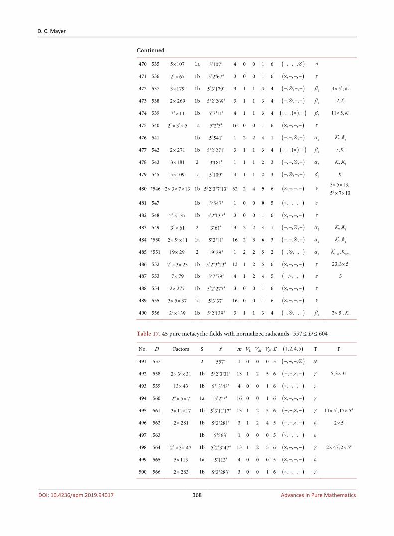
Table 16. 45 pure metacyclic fields with normalized radicands 509 556D≤ ≤ .
No. D Factors S f4 m VL VM VN E ( )1,2,4,5 T P
446 509 1b 2 45 509 1 1 1 2 3 ( ), , ,− ⊗ − − 2δ
447 510 2 3 5 17× × × 1a 6 4 4 45 2 3 17 64 1 2 5 6 ( ), , ,× − − − γ 2 3,2 17× ×
448 511 7 73× 1b 2 4 45 7 73 4 0 0 1 6 ( ), , ,× − − − γ
449 513 33 19× 1b 2 4 45 3 19 3 1 2 4 5 ( ), , ,− × − − ε 23 5×
450 514 2 257× 1b 2 4 45 2 257 4 0 0 1 6 ( ), , ,× − − − γ
451 515 5 103× 1a 6 45 103 4 0 0 0 5 ( ), , ,× − − − ε
452 516 22 3 43× × 1b 2 4 4 45 2 3 43 12 1 2 5 6 ( ), , ,× − − − γ 2 42 3 ,2 5× ×
453 *517 11 47× 1b 2 4 45 11 47 3 2 3 6 3 ( ), , ,− − ⊗ − 1β 2211 5 ,× K
454 518 2 7 37× × 2 4 4 42 7 37 4 0 0 1 6 ( ), , ,× − − − γ
455 519 3 173× 1b 2 4 45 3 173 3 0 0 1 6 ( ), , ,× − − − γ
456 520 32 5 13× × 1a 6 4 45 2 13 16 1 2 4 5 ( ), , ,× − − − ε 2
457 521 1b 2 45 521 1 1 2 3 4 ( ), , ,− − ⊗ − 1δ 2K
458 522 22 3 29⋅× × 1b 2 4 4 45 2 3 29 13 1 2 5 6 ( ), , ,− × − − γ 2,29 5×
459 523 1b 2 45 523 1 0 0 0 5 ( ), , ,× − − − ε
460 524 22 131× 2 4 42 131 1 1 1 2 3 ( ), , ,− − ⊗ − 2α 1,K
461 525 23 5 7× × 1a 6 4 45 3 7 16 0 0 1 6 ( ), , ,× − − − γ
462 526 2 263× 2 4 42 263 1 0 0 0 5 ( ), , ,× − − − ε
463 527 17 31× 1b 2 4 45 17 31 3 1 1 3 4 ( )( ), , ,− − × − 2β 5,
464 528 42 3 11× × 1b 2 4 4 45 2 3 11 13 1 2 5 6 ( ), , ,− − × − γ 32 5,3 5× ×
465 530 2 5 53× × 1a 6 4 45 2 53 16 0 0 1 6 ( ), , ,× − − − γ
466 531 23 59× 1b 2 4 45 3 59 3 1 1 3 4 ( ), , ,− ⊗ − − 2β 3,
467 *532 22 7 19× × 2 4 4 42 7 19 4 1 2 4 5 ( ), , ,− × − − ε 2 7×
468 533 13 41× 1b 2 4 45 13 41 3 1 1 3 4 ( )( ), , ,− − × − 2β 213 5 ,×
469 534 2 3 89× × 1b 2 4 4 45 2 3 89 13 1 2 5 6 ( ), , ,− × − − γ 3,89 5×
D. C. Mayer
DOI: 10.4236/apm.2019.94017 368 Advances in Pure Mathematics
Continued
470 535 5 107× 1a 6 45 107 4 0 0 1 6 ( ), , ,− − − ⊗ η
471 536 32 67× 1b 2 4 45 2 67 3 0 0 1 6 ( ), , ,× − − − γ
472 537 3 179× 1b 2 4 45 3 179 3 1 1 3 4 ( ), , ,− ⊗ − − 2β 23 5 ,×
473 538 2 269× 1b 2 4 45 2 269 3 1 1 3 4 ( ), , ,− ⊗ − − 2β 2,
474 539 27 11× 1b 2 4 45 7 11 4 1 1 3 4 ( )( ), , ,− − × − 2β 11 5,×
475 540 2 32 3 5× × 1a 6 4 45 2 3 16 0 0 1 6 ( ), , ,× − − − γ
476 541 1b 2 45 541 1 2 2 4 1 ( ), , ,− − ⊗ − 2α 1,K
477 542 2 271× 1b 2 4 45 2 271 3 1 1 3 4 ( )( ), , ,− − × − 2β 5,
478 543 3 181× 2 4 43 181 1 1 1 2 3 ( ), , ,− − ⊗ − 2α 1,K
479 545 5 109× 1a 6 45 109 4 1 1 2 3 ( ), , ,− ⊗ − − 2δ
480 *546 2 3 7 13× × × 1b 2 4 4 4 45 2 3 7 13 52 2 4 9 6 ( ), , ,× − − − γ 2
3 5 13,5 7 13× ×
× ×
481 547 1b 2 45 547 1 0 0 0 5 ( ), , ,× − − − ε
482 548 22 137× 1b 2 4 45 2 137 3 0 0 1 6 ( ), , ,× − − − γ
483 549 23 61× 2 4 43 61 3 2 2 4 1 ( ), , ,− − ⊗ − 2α 1,K
484 *550 22 5 11× × 1a 6 4 45 2 11 16 2 3 6 3 ( ), , ,− − ⊗ − 2α 1,K
485 *551 19 29× 2 4 419 29 1 2 2 5 2 ( ), , ,− ⊗ − − 3α (19) (29),
486 552 32 3 23× × 1b 2 4 4 45 2 3 23 13 1 2 5 6 ( ), , ,× − − − γ 23,3 5×
487 553 7 79× 1b 2 4 45 7 79 4 1 2 4 5 ( ), , ,− × − − ε 5
488 554 2 277× 1b 2 4 45 2 277 3 0 0 1 6 ( ), , ,× − − − γ
489 555 3 5 37× × 1a 6 4 45 3 37 16 0 0 1 6 ( ), , ,× − − − γ
490 556 22 139× 1b 2 4 45 2 139 3 1 1 3 4 ( ), , ,− ⊗ − − 2β 22 5 ,×
Table 17. 45 pure metacyclic fields with normalized radicands 557 604D≤ ≤ .
No. D Factors S f4 m VL VM VN E ( )1,2,4,5 T P
491 557 2 4557 1 0 0 0 5 ( ), , ,− − − ⊗ ϑ
492 558 22 3 31× × 1b 2 4 4 45 2 3 31 13 1 2 5 6 ( ), , ,− − × − γ 5,3 31×
493 559 13 43× 1b 2 4 45 13 43 4 0 0 1 6 ( ), , ,× − − − γ
494 560 42 5 7× × 1a 6 4 45 2 7 16 0 0 1 6 ( ), , ,× − − − γ
495 561 3 11 17× × 1b 2 4 4 45 3 11 17 13 1 2 5 6 ( ), , ,− − × − γ 3 411 5 ,17 5× ×
496 562 2 281× 1b 2 4 45 2 281 3 1 2 4 5 ( ), , ,− − × − ε 2 5×
497 563 1b 2 45 563 1 0 0 0 5 ( ), , ,× − − − ε
498 564 22 3 47× × 1b 2 4 4 45 2 3 47 13 1 2 5 6 ( ), , ,× − − − γ 22 47,2 5× ×
499 565 5 113× 1a 6 45 113 4 0 0 0 5 ( ), , ,× − − − ε
500 566 2 283× 1b 2 4 45 2 283 3 0 0 1 6 ( ), , ,× − − − γ

D. C. Mayer
DOI: 10.4236/apm.2019.94017 369 Advances in Pure Mathematics
Continued
501 567 43 7× 1b 2 4 45 3 7 4 0 0 1 6 ( ), , ,× − − − γ
502 568 32 71× 2 4 42 71 1 1 1 2 3 ( ), , ,− − ⊗ − 2α 1,K
503 569 1b 2 45 569 1 1 1 2 3 ( ), , ,− ⊗ − − 2δ
504 *570 2 3 5 19× × × 1a 6 4 4 45 2 3 19 64 1 2 5 6 ( ), , ,− × − − γ 4 42 3,2 5× ×
505 571 1b 2 45 571 1 2 2 4 1 ( ), , ,− − ⊗ − 2α 1,K
506 572 22 11 13× × 1b 2 4 4 45 2 11 13 13 2 3 6 3 ( ), , ,− − ⊗ − 1β 2 322 13 5 ,× × K
507 573 3 191× 1b 2 4 45 3 191 3 1 1 3 4 ( )( ), , ,− − × − 2β 5,
508 *574 2 7 41× × 2 4 4 42 7 41 4 1 1 3 4 ( )( ), , ,− − × − 2β 41,
509 575 25 23× 1a 6 45 23 4 0 0 0 5 ( ), , ,× − − − ε
510 577 1b 2 45 577 1 0 0 0 5 ( ), , ,× − − − ε
511 579 3 193× 1b 2 4 45 3 193 4 0 0 1 6 ( ), , ,× − − − γ
512 580 22 5 29× × 1a 6 4 45 2 29 16 1 1 3 4 ( ), , ,− ⊗ − − 2β 42 5,×
513 581 7 83× 1b 2 4 45 7 83 4 0 0 1 6 ( ), , ,× − − − γ
514 582 2 3 97× × 2 4 4 42 3 97 3 0 0 1 6 ( ), , ,× − − − γ
515 583 11 53× 1b 2 4 45 11 53 3 1 1 3 4 ( )( ), , ,− − × − 2β 53 5,×
516 584 32 73× 1b 2 4 45 2 73 3 0 0 1 6 ( ), , ,× − − − γ
517 585 23 5 13× × 1a 6 4 45 3 13 16 0 0 1 6 ( ), , ,× − − − γ
518 586 2 293× 1b 2 4 45 2 293 4 1 2 4 5 ( ), , ,× − − − ε 2
519 587 1b 2 45 587 1 0 0 0 5 ( ), , ,× − − − ε
520 589 19 31× 1b 2 4 45 19 31 3 2 2 5 2 ( )( ), , ,− ⊗ × − 3α (19) (31),
521 *590 2 5 59× × 1a 6 4 45 2 59 16 2 3 7* 4 ( ), , ,− ⊗ − − 2β 5,
522 591 3 197× 1b 2 4 45 3 197 3 0 0 1 6 ( ), , ,× − − − γ
523 592 42 37× 1b 2 4 45 2 37 3 0 0 1 6 ( ), , ,× − − − γ
524 593 2 4593 1 0 0 0 5 ( ), , ,− − − ⊗ ϑ
525 594 32 3 11× × 1b 2 4 4 45 2 3 11 13 1 2 5 6 ( ), , ,− − × − γ 211,3 5×
526 595 5 7 17× × 1a 6 4 45 7 17 16 0 0 1 6 ( ), , ,× − − − γ
527 596 22 149× 1b 2 4 45 2 149 4 1 2 4 5 ( ), , ,− × − − ε 22 5×
528 597 3 199× 1b 2 4 45 3 199 4 1 1 3 4 ( ), , ,− ⊗ − − 2β 43 5,×
529 598 2 13 23× × 1b 2 4 4 45 2 13 23 13 1 2 5 6 ( ), , ,× − − − γ 4 32 5,13 5× ×
530 599 2 4599 1 1 1 2 3 ( ), , ,− ⊗ − × 2δ
531 600 3 22 3 5× × 1a 6 4 45 2 3 16 0 0 1 6 ( ), , ,× − − − γ
532 601 2 4601 1 1 1 2 3 ( ), , ,− − ⊗ × 2α 2,K
533 *062 2 7 43× × 1b 2 4 4 45 2 7 43 16 1 2 5 6 ( ), , ,× − − − γ 2, 7
534 603 23 67× 1b 2 4 45 3 67 3 0 0 1 6 ( ), , ,× − − − γ
535 604 22 151× 1b 2 4 45 2 151 4 1 2 4 5 ( ), , ,− − ⊗ − 1β 12,K
D. C. Mayer
DOI: 10.4236/apm.2019.94017 370 Advances in Pure Mathematics
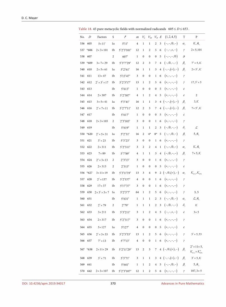
Table 18. 45 pure metacyclic fields with normalized radicands 605 653D≤ ≤ .
No. D Factors S f4 m VL VM VN E ( )1,2,4,5 T P
536 605 25 11× 1a 6 45 11 4 1 1 2 3 ( ), , ,− − ⊗ − 2α 1,K
537 *606 2 3 101× × 1b 2 4 4 45 2 3 101 12 1 2 5 6 ( ), , ,− − × − γ 2 5,101×
538 607 2 4607 1 0 0 0 5 ( ), , ,− − − ⊗ ϑ
539 *609 3 7 29× × 1b 2 4 4 45 3 7 29 12 2 3 7 4 ( ), , ,− ⊗ − − 2β 27 5,×
540 610 2 5 61× × 1a 6 4 45 2 61 16 1 1 3 4 ( )( ), , ,− − × − 2β 22 5 ,×
541 611 13 47× 1b 2 4 45 13 47 3 0 0 1 6 ( ), , ,× − − − γ
542 612 2 22 3 17× × 1b 2 4 4 45 2 3 17 13 1 2 5 6 ( ), , ,× − − − γ 217,3 5×
543 613 1b 2 45 613 1 0 0 0 5 ( ), , ,× − − − ε
544 614 2 307× 1b 2 4 45 2 307 4 1 2 4 5 ( ), , ,× − − − ε 2
545 615 3 5 41× × 1a 6 4 45 3 41 16 1 1 3 4 ( )( ), , ,− − × − 2β 3,
546 616 32 7 11× × 1b 2 4 4 45 2 7 11 12 2 3 7 4 ( )( ), , ,− − × − 2β 27 5 ,×
547 617 1b 2 45 617 1 0 0 0 5 ( ), , ,× − − − ε
548 618 2 3 103× × 2 4 4 42 3 103 3 0 0 1 6 ( ), , ,× − − − γ
549 619 1b 2 45 619 1 1 1 2 3 ( ), , ,− ⊗ − − 2δ
550 *620 22 5 31× × 1a 6 4 45 2 31 16 2 4* 8* 5 ( ), , ,− − ⊗ − 1β 15,K
551 621 33 23× 1b 2 4 45 3 23 3 0 0 1 6 ( ), , ,× − − − γ
552 622 2 311× 1b 2 4 45 2 311 3 2 2 4 1 ( ), , ,− − ⊗ − 2α 1,K
553 623 7 89× 1b 2 4 45 7 89 4 1 1 3 4 ( ), , ,− ⊗ − − 2β 7 5,×
554 624 42 3 13× × 2 4 4 42 3 13 3 0 0 1 6 ( ), , ,× − − − γ
555 626 2 313× 2 4 42 313 1 0 0 0 5 ( ), , ,× − − − ε
556 *627 3 11 19× × 1b 2 4 4 45 3 11 19 13 3 4 9 2 ( )( ), , ,− ⊗ × − 3α (11) (19),
557 628 22 157× 1b 2 4 45 2 157 4 0 0 1 6 ( ), , ,× − − − γ
558 629 17 37× 1b 2 4 45 17 37 3 0 0 1 6 ( ), , ,× − − − γ
559 630 22 3 5 7× × × 1a 6 4 4 45 2 3 7 64 1 2 5 6 ( ), , ,× − − − γ 3, 5
560 631 1b 2 45 631 1 1 1 2 3 ( ), , ,− − ⊗ − 2α 1,K
561 632 32 79× 2 4 42 79 1 1 1 2 3 ( ), , ,− ⊗ − − 2δ
562 633 3 211× 1b 2 4 45 3 211 3 1 2 4 5 ( ), , ,− − × − ε 3 5×
563 634 2 317× 1b 2 4 45 2 317 3 0 0 1 6 ( ), , ,× − − − γ
564 635 5 127× 1a 6 45 127 4 0 0 0 5 ( ), , ,× − − − ε
565 636 22 3 53× × 1b 2 4 4 45 2 3 53 13 1 2 5 6 ( ), , ,× − − − γ 23 5,53×
566 637 27 13× 1b 2 4 45 7 13 4 0 0 1 6 ( ), , ,× − − − γ
567 *638 2 11 29× × 1b 2 4 4 45 2 11 29 13 2 3 7 4 ( )( ), , ,− ⊗ × − 2β 4
4(11) (29)
2 11 5,× ×
×
568 639 23 71× 1b 2 4 45 3 71 3 1 1 3 4 ( )( ), , ,− − × − 2β 23 5,×
569 641 1b 2 45 641 1 1 2 4 5 ( ), , ,− − ⊗ − 1β 25,K
570 642 2 3 107× × 1b 2 4 4 45 2 3 107 12 1 2 5 6 ( ), , ,× − − − γ 107,3 5×

D. C. Mayer
DOI: 10.4236/apm.2019.94017 371 Advances in Pure Mathematics
Continued
571 643 2 4643 1 0 0 0 5 ( ), , ,− − − ⊗ ϑ
572 644 22 7 23× × 1b 2 4 4 45 2 7 23 12 1 2 5 6 ( ), , ,× − − − γ 2 5,7 5× ×
573 645 3 5 43× × 1a 6 4 45 3 43 16 1 2 4 5 ( ), , ,× − − − ε 43
574 646 2 17 19× × 1b 2 4 4 45 2 17 19 13 1 2 5 6 ( ), , ,− × − − γ 2 5,17×
575 647 1b 2 45 647 1 0 0 0 5 ( ), , ,× − − − ε
576 *649 11 59× 2 4 411 59 1 2 2 5 2 ( )( ), , ,− ⊗ × − 3α (11) (59),
577 650 22 5 13× × 1a 6 4 45 2 13 16 0 0 1 6 ( ), , ,× − − − γ
578 651 3 7 31× × 2 4 4 43 7 31 4 1 1 3 4 ( )( ), , ,− − × − 2β 23 7,×
579 652 22 163× 1b 2 4 45 2 163 3 1 2 4 5 ( ), , ,× − − − ε 5
580 653 1b 2 45 653 1 0 0 0 5 ( ), , ,× − − − ε
Table 19. 44 pure metacyclic fields with normalized radicands 654 701D≤ ≤ .
No. D Factors S f4 m VL VM VN E ( )1,2,4,5 T P
581 654 2 3 109× × 1b 2 4 4 45 2 3 109 13 1 2 5 6 ( ), , ,× − − − γ 3 5,109×
582 655 5 131× 1a 6 45 131 4 1 1 2 3 ( ), , ,− − ⊗ − 2α 1,K
583 656 42 41× 1b 2 4 45 2 41 3 2 2 4 1 ( ), , ,− − ⊗ − 2α 1,K
584 657 23 73× 2 4 43 73 1 0 0 0 5 ( ), , ,× − − − ε
585 658 2 7 47× × 1b 2 4 4 45 2 7 47 12 1 2 5 6 ( ), , ,× − − − γ 2 5,47 5× ×
586 659 1b 2 45 659 1 1 1 2 3 ( ), , ,− ⊗ − − 2δ
587 *660 22 3 5 11× × × 1a 6 4 4 45 2 3 11 64 1 2 5 6 ( ), , ,− − × − γ 2 5,5 11× ×
588 661 1b 2 45 661 1 1 1 2 3 ( ), , ,− − ⊗ − 2α 1,K
589 662 2 331× 1b 2 4 45 2 331 3 1 1 3 4 ( )( ), , ,− − × − 2β 42 5,×
590 663 3 13 17× × 1b 2 4 4 45 3 13 17 13 1 2 5 6 ( ), , ,× − − − γ 2 23 5,13 5× ×
591 664 32 83× 1b 2 4 45 2 83 3 1 2 4 5 ( ), , ,× − − − ε 22 5×
592 *665 5 7 19× × 1a 6 4 45 7 19 16 1 1 3 4 ( ), , ,− ⊗ − − 2β 7,
593 666 22 3 37× × 1b 2 4 4 45 2 3 37 13 1 2 5 6 ( ), , ,× − − − γ 237,2 5×
594 667 23 29× 1b 2 4 45 23 29 3 1 1 3 4 ( ), , ,− ⊗ − − 2β 223 5 ,×
595 668 22 167× 2 4 42 167 1 0 0 0 5 ( ), , ,× − − − ε
596 669 3 223× 1b 2 4 45 3 223 3 0 0 1 6 ( ), , ,× − − − γ
597 670 2 5 67× × 1a 6 4 45 2 67 16 1 2 4 5 ( ), , ,× − − − ε 2
598 *671 11 61× 1b 2 4 45 11 61 3 3 4 8 1 ( ), , ,− − ⊗ − 2α (11) (61)
2(11),2 (61),1
,
K K
599 673 1b 2 45 673 1 0 0 0 5 ( ), , ,× − − − ε
600 674 2 337× 2 4 42 337 1 0 0 0 5 ( ), , ,× − − − ε
601 677 1b 2 45 677 1 0 0 0 5 ( ), , ,× − − − ε
602 678 2 3 113× × 1b 2 4 4 45 2 3 113 13 1 2 5 6 ( ), , ,× − − − γ 2 42 5,3 5× ×
603 679 7 97× 1b 2 4 45 7 97 4 0 0 1 6 ( ), , ,× − − − γ
D. C. Mayer
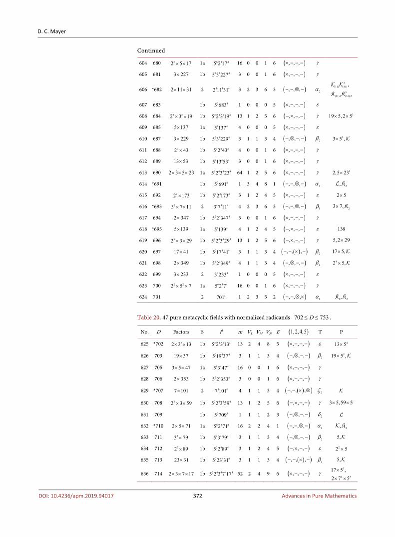
DOI: 10.4236/apm.2019.94017 372 Advances in Pure Mathematics
Continued
604 680 32 5 17× × 1a 6 4 45 2 17 16 0 0 1 6 ( ), , ,× − − − γ
605 681 3 227× 1b 2 4 45 3 227 3 0 0 1 6 ( ), , ,× − − − γ
606 *682 2 11 31× × 2 4 4 42 11 31 3 2 3 6 3 ( ), , ,− − ⊗ − 2α 3
(11) (31)
3(11),1 (31),2
,
K K
607 683 1b 2 45 683 1 0 0 0 5 ( ), , ,× − − − ε
608 684 2 22 3 19× × 1b 2 4 4 45 2 3 19 13 1 2 5 6 ( ), , ,− × − − γ 319 5,2 5× ×
609 685 5 137× 1a 6 45 137 4 0 0 0 5 ( ), , ,× − − − ε
610 687 3 229× 1b 2 4 45 3 229 3 1 1 3 4 ( ), , ,− ⊗ − − 2β 23 5 ,×
611 688 42 43× 1b 2 4 45 2 43 4 0 0 1 6 ( ), , ,× − − − γ
612 689 13 53× 1b 2 4 45 13 53 3 0 0 1 6 ( ), , ,× − − − γ
613 690 2 3 5 23× × × 1a 6 4 4 45 2 3 23 64 1 2 5 6 ( ), , ,× − − − γ 22,5 23×
614 *691 1b 2 45 691 1 3 4 8 1 ( ), , ,− − ⊗ − 2α 2,K
615 692 22 173× 1b 2 4 45 2 173 3 1 2 4 5 ( ), , ,× − − − ε 2 5×
616 *693 23 7 11× × 2 4 4 43 7 11 4 2 3 6 3 ( ), , ,− − ⊗ − 1β 23 7,× K
617 694 2 347× 1b 2 4 45 2 347 3 0 0 1 6 ( ), , ,× − − − γ
618 *695 5 139× 1a 6 45 139 4 1 2 4 5 ( ), , ,− × − − ε 139
619 696 32 3 29× × 1b 2 4 4 45 2 3 29 13 1 2 5 6 ( ), , ,− × − − γ 5,2 29×
620 697 17 41× 1b 2 4 45 17 41 3 1 1 3 4 ( )( ), , ,− − × − 2β 17 5,×
621 698 2 349× 1b 2 4 45 2 349 4 1 1 3 4 ( ), , ,− ⊗ − − 2β 42 5,×
622 699 3 233× 2 4 43 233 1 0 0 0 5 ( ), , ,× − − − ε
623 700 2 22 5 7× × 1a 6 4 45 2 7 16 0 0 1 6 ( ), , ,× − − − γ
624 701 2 4701 1 2 3 5 2 ( ), , ,− − ⊗ × 1α 1 2,K K
Table 20. 47 pure metacyclic fields with normalized radicands 702 753D≤ ≤ .
No. D Factors S f4 m VL VM VN E ( )1,2,4,5 T P
625 *702 32 3 13× × 1b 2 4 4 45 2 3 13 13 2 4 8 5 ( ), , ,× − − − ε 413 5×
626 703 19 37× 1b 2 4 45 19 37 3 1 1 3 4 ( ), , ,− ⊗ − − 2β 219 5 ,×
627 705 3 5 47× × 1a 6 4 45 3 47 16 0 0 1 6 ( ), , ,× − − − γ
628 706 2 353× 1b 2 4 45 2 353 3 0 0 1 6 ( ), , ,× − − − γ
629 *707 7 101× 2 4 47 101 4 1 1 3 4 ( )( ), , ,− − × ⊗ 2ζ
630 708 22 3 59× × 1b 2 4 4 45 2 3 59 13 1 2 5 6 ( ), , ,− × − − γ 3 5,59 5× ×
631 709 1b 2 45 709 1 1 1 2 3 ( ), , ,− ⊗ − − 2δ
632 *710 2 5 71× × 1a 6 4 45 2 71 16 2 2 4 1 ( ), , ,− − ⊗ − 2α 2,K
633 711 23 79× 1b 2 4 45 3 79 3 1 1 3 4 ( ), , ,− ⊗ − − 2β 5,
634 712 32 89× 1b 2 4 45 2 89 3 1 2 4 5 ( ), , ,− × − − ε 22 5×
635 713 23 31× 1b 2 4 45 23 31 3 1 1 3 4 ( )( ), , ,− − × − 2β 5,
636 714 2 3 7 17× × × 1b 2 4 4 4 45 2 3 7 17 52 2 4 9 6 ( ), , ,× − − − γ 3
2 3
17 5 ,2 7 5×
× ×
D. C. Mayer
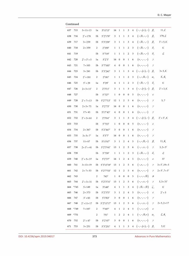
DOI: 10.4236/apm.2019.94017 373 Advances in Pure Mathematics
Continued
637 715 5 11 13× × 1a 6 4 45 11 13 16 1 1 3 4 ( )( ), , ,− − × − 2β 11,
638 716 22 179× 1b 2 4 45 2 179 3 1 1 3 4 ( ), , ,− ⊗ − − 2β 179,
639 717 3 239× 1b 2 4 45 3 239 3 1 1 3 4 ( ), , ,− ⊗ − − 2β 23 5,×
640 718 2 359× 2 4 42 359 1 1 1 2 3 ( ), , ,− ⊗ − − 2δ
641 719 1b 2 45 719 1 1 1 2 3 ( ), , ,− ⊗ − − 2δ
642 720 4 22 3 5× × 1a 6 4 45 2 3 16 0 0 1 6 ( ), , ,× − − − γ
643 721 7 103× 1b 2 4 45 7 103 4 0 0 1 6 ( ), , ,× − − − γ
644 723 3 241× 1b 2 4 45 3 241 3 1 1 3 4 ( )( ), , ,− − × − 2β 3 5,×
645 724 22 181× 2 4 42 181 1 1 1 2 3 ( ), , ,− − ⊗ − 2α 1,K
646 725 25 29× 1a 6 45 29 4 1 1 2 3 ( ), , ,− ⊗ − − 2δ
647 726 22 3 11× × 2 4 4 42 3 11 3 1 1 3 4 ( )( ), , ,− − × − 2β 22 3,×
648 727 1b 2 45 727 1 0 0 0 5 ( ), , ,× − − − ε
649 728 32 7 13× × 1b 2 4 4 45 2 7 13 12 1 2 5 6 ( ), , ,× − − − γ 5, 7
650 730 2 5 73× × 1a 6 4 45 2 73 16 0 0 1 6 ( ), , ,× − − − γ
651 731 17 43× 1b 2 4 45 17 43 4 0 0 1 6 ( ), , ,× − − − γ
652 732 22 3 61× × 2 4 4 42 3 61 3 1 1 3 4 ( )( ), , ,− − × − 2β 3 22 3 ,×
653 733 1b 2 45 733 1 0 0 0 5 ( ), , ,× − − − ε
654 734 2 367× 1b 2 4 45 2 367 3 0 0 1 6 ( ), , ,× − − − γ
655 735 23 5 7× × 1a 6 4 45 3 7 16 0 0 1 6 ( ), , ,× − − − γ
656 737 11 67× 1b 2 4 45 11 67 3 1 2 4 5 ( ), , ,− − ⊗ − 1β 111,K
657 738 22 3 41× × 1b 2 4 4 45 2 3 41 13 1 2 5 6 ( ), , ,− − × − γ 23, 2 5×
658 739 1b 2 45 739 1 1 1 2 3 ( ), , ,− ⊗ − − 2δ
659 740 22 5 37× × 1a 6 4 45 2 37 16 1 2 4 5 ( ), , ,× − − − ε 37
660 741 3 13 19× × 1b 2 4 4 45 3 13 19 13 1 2 5 6 ( ), , ,− × − − γ 23 5 ,19 5× ×
661 742 2 7 53× × 1b 2 4 4 45 2 7 53 12 1 2 5 6 ( ), , ,× − − − γ 2 22 5 ,7 5× ×
662 743 2 4743 1 0 0 0 5 ( ), , ,− − − ⊗ ϑ
663 744 32 3 31× × 1b 2 4 4 45 2 3 31 13 1 2 5 6 ( ), , ,− − × − γ 25,3 31×
664 *745 5 149× 1a 6 45 149 4 1 1 3 4 ( ), , ,− ⊗ − ⊗ 2ζ
665 746 2 373× 1b 2 4 45 2 373 3 1 2 4 5 ( ), , ,× − − − ε 42 5×
666 747 23 83× 1b 2 4 45 3 83 3 0 0 1 6 ( ), , ,× − − − γ
667 748 22 11 17× × 1b 2 4 4 45 2 11 17 13 1 2 5 6 ( ), , ,− − × − γ 2 5,2 17× ×
668 *749 7 107× 2 4 47 107 4 1 2 4 5 ( ), , ,− − − × ε
669 *751 2 4751 1 2 2 4 1 ( ), , ,− − ⊗ × 2α 1,K
670 752 42 47× 1b 2 4 45 2 47 3 0 0 1 6 ( ), , ,× − − − γ
671 753 3 251× 1b 2 4 45 3 251 4 1 1 3 4 ( )( ), , ,− − × − 2β 5,
D. C. Mayer
DOI: 10.4236/apm.2019.94017 374 Advances in Pure Mathematics
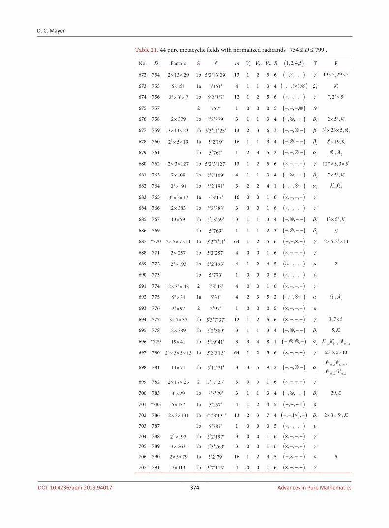
Table 21. 44 pure metacyclic fields with normalized radicands 754 799D≤ ≤ .
No. D Factors S f4 m VL VM VN E ( )1,2,4,5 T P
672 754 2 13 29× × 1b 2 4 4 45 2 13 29 13 1 2 5 6 ( ), , ,− × − − γ 13 5,29 5× ×
673 755 5 151× 1a 6 45 151 4 1 1 3 4 ( )( ), , ,− − × ⊗ 2ζ
674 756 2 32 3 7× × 1b 2 4 4 45 2 3 7 12 1 2 5 6 ( ), , ,× − − − γ 3 27, 2 5×
675 757 2 4757 1 0 0 0 5 ( ), , ,− − − ⊗ ϑ
676 758 2 379× 1b 2 4 45 2 379 3 1 1 3 4 ( ), , ,− ⊗ − − 2β 22 5 ,×
677 759 3 11 23× × 1b 2 4 4 45 3 11 23 13 2 3 6 3 ( ), , ,− − ⊗ − 1β 223 23 5,× × K
678 760 32 5 19× × 1a 6 4 45 2 19 16 1 1 3 4 ( ), , ,− ⊗ − − 2β 42 19,×
679 761 1b 2 45 761 1 2 3 5 2 ( ), , ,− − ⊗ − 1α 1 2,K K
680 762 2 3 127× × 1b 2 4 4 45 2 3 127 13 1 2 5 6 ( ), , ,× − − − γ 3127 5,3 5× ×
681 763 7 109× 1b 2 4 45 7 109 4 1 1 3 4 ( ), , ,− ⊗ − − 2β 27 5 ,×
682 764 22 191× 1b 2 4 45 2 191 3 2 2 4 1 ( ), , ,− − ⊗ − 2α 2,K
683 765 23 5 17× × 1a 6 4 45 3 17 16 0 0 1 6 ( ), , ,× − − − γ
684 766 2 383× 1b 2 4 45 2 383 3 0 0 1 6 ( ), , ,× − − − γ
685 767 13 59× 1b 2 4 45 13 59 3 1 1 3 4 ( ), , ,− ⊗ − − 2β 213 5 ,×
686 769 1b 2 45 769 1 1 1 2 3 ( ), , ,− ⊗ − − 2δ
687 *770 2 5 7 11× × × 1a 6 4 4 45 2 7 11 64 1 2 5 6 ( ), , ,− − × − γ 22 5,2 11× ×
688 771 3 257× 1b 2 4 45 3 257 4 0 0 1 6 ( ), , ,× − − − γ
689 772 22 193× 1b 2 4 45 2 193 4 1 2 4 5 ( ), , ,× − − − ε 2
690 773 1b 2 45 773 1 0 0 0 5 ( ), , ,× − − − ε
691 774 22 3 43× × 2 4 4 42 3 43 4 0 0 1 6 ( ), , ,× − − − γ
692 775 25 31× 1a 6 45 31 4 2 3 5 2 ( ), , ,− − ⊗ − 1α 1 2,K K
693 776 32 97× 2 4 42 97 1 0 0 0 5 ( ), , ,× − − − ε
694 777 3 7 37× × 1b 2 4 4 45 3 7 37 12 1 2 5 6 ( ), , ,× − − − γ 3,7 5×
695 778 2 389× 1b 2 4 45 2 389 3 1 1 3 4 ( ), , ,− ⊗ − − 2β 5,
696 *779 19 41× 1b 2 4 45 19 41 3 3 4 8 1 ( ), , ,− ⊗ ⊗ − 2α (19) (41) (41),1,K
697 780 22 3 5 13× × × 1a 6 4 4 45 2 3 13 64 1 2 5 6 ( ), , ,× − − − γ 2 5,5 13× ×
698 781 11 71× 1b 2 4 45 11 71 3 3 5 9 2 ( ), , ,− − ⊗ − 1α 4
(11),1 (71),1
2(11),2 (71),2
,K K
K K
699 782 2 17 23× × 2 4 4 42 17 23 3 0 0 1 6 ( ), , ,× − − − γ
700 783 33 29× 1b 2 4 45 3 29 3 1 1 3 4 ( ), , ,− ⊗ − − 2β 29,
701 *785 5 157× 1a 6 45 157 4 1 2 4 5 ( ), , ,− − − × ε
702 786 2 3 131× × 1b 2 4 4 45 2 3 131 13 2 3 7 4 ( )( ), , ,− − × − 2β 22 3 5 ,× ×
703 787 1b 2 45 787 1 0 0 0 5 ( ), , ,× − − − ε
704 788 22 197× 1b 2 4 45 2 197 3 0 0 1 6 ( ), , ,× − − − γ
705 789 3 263× 1b 2 4 45 3 263 3 0 0 1 6 ( ), , ,× − − − γ
706 790 2 5 79× × 1a 6 4 45 2 79 16 1 2 4 5 ( ), , ,− × − − ε 5
707 791 7 113× 1b 2 4 45 7 113 4 0 0 1 6 ( ), , ,× − − − γ

D. C. Mayer
DOI: 10.4236/apm.2019.94017 375 Advances in Pure Mathematics
Continued
708 792 3 22 3 11× × 1b 2 4 4 45 2 3 11 13 1 2 5 6 ( ), , ,− − × − γ 2 5,11 5× ×
709 793 13 61× 2 4 413 61 1 1 2 4 5 ( ), , ,− − ⊗ − 1β 261,K
710 794 2 397× 1b 2 4 45 2 397 3 0 0 1 6 ( ), , ,× − − − γ
711 795 3 5 53× × 1a 6 4 45 3 53 16 0 0 1 6 ( ), , ,× − − − γ
712 796 22 199× 1b 2 4 45 2 199 4 1 1 3 4 ( ), , ,− ⊗ − − 2β 2 5,×
713 797 1b 2 45 797 1 0 0 0 5 ( ), , ,× − − − ε
714 *798 2 3 7 19× × × 1b 2 4 4 4 45 2 3 7 19 52 2 4 9 6 ( ), , ,− × − − γ 43 19,7 5× ×
715 799 17 47× 2 4 417 47 1 0 0 0 5 ( ), , ,× − − − ε
Table 22. 46 pure metacyclic fields with normalized radicands 801 848D≤ ≤ .
No. D Factors S f4 m VL VM VN E ( )1,2,4,5 T P
716 801 23 89× 2 4 43 89 1 1 1 2 3 ( ), , ,− ⊗ − − 2δ
717 802 2 401× 1b 2 4 45 2 401 4 1 1 3 4 ( )( ), , ,− − × − 2β 22 5,×
718 803 11 73× 1b 2 4 45 11 73 3 1 1 3 4 ( )( ), , ,− − × − 2β 273 5 ,×
719 804 22 3 67× × 1b 2 4 4 45 2 3 67 13 1 2 5 6 ( ), , ,× − − − γ 33, 2 5×
720 805 5 7 23× × 1a 6 4 45 7 23 16 0 0 1 6 ( ), , ,× − − − γ
721 806 2 13 31× × 1b 2 4 4 45 2 13 31 13 2 3 6 3 ( ), , ,− − ⊗ − 1β 2231 5 ,× K
722 807 3 269× 2 4 43 269 1 1 1 2 3 ( ), , ,− ⊗ − − 2δ
723 *808 32 101× 1b 2 4 45 2 101 4 2 2 4 1 ( ), , ,− − ⊗ − 2α 1,K
724 809 1b 2 45 809 1 1 1 2 3 ( ), , ,− ⊗ − − 2δ
725 810 42 3 5× × 1a 6 4 45 2 3 16 0 0 1 6 ( ), , ,× − − − γ
726 811 1b 2 45 811 1 1 1 2 3 ( ), , ,− − ⊗ − 2α 1,K
727 812 22 7 29× × 1b 2 4 4 45 2 7 29 12 1 2 5 6 ( ), , ,− × − − γ 229,7 5×
728 813 3 271× 1b 2 4 45 3 271 3 1 1 3 4 ( )( ), , ,− − × − 2β 5,
729 814 2 11 37× × 1b 2 4 4 45 2 11 37 13 2 3 6 3 ( ), , ,− − ⊗ − 1β 2211 37 5,× × K
730 815 5 163× 1a 6 45 163 4 0 0 0 5 ( ), , ,× − − − ε
731 816 42 3 17× × 1b 2 4 4 45 2 3 17 13 1 2 5 6 ( ), , ,× − − − γ 2 32 5 ,3 5× ×
732 817 19 43× 1b 2 4 45 19 43 4 1 1 3 4 ( ), , ,− ⊗ − − 2β 219 5,×
733 818 2 409× 2 4 42 409 1 1 1 2 3 ( ), , ,− ⊗ − − 2δ
734 819 23 7 13× × 1b 2 4 4 45 3 7 13 12 1 2 5 6 ( ), , ,× − − − γ 213,7 5×
735 820 22 5 41× × 1a 6 4 45 2 41 16 2 2 4 1 ( ), , ,− − ⊗ − 2α 1,K
736 821 1b 2 45 821 1 1 1 2 3 ( ), , ,− − ⊗ − 2α 2,K
737 822 2 3 137× × 1b 2 4 4 45 2 3 137 13 2 4 8 5 ( ), , ,× − − − ε 33 137 5× ×
738 823 1b 2 45 823 1 0 0 0 5 ( ), , ,× − − − ε
739 824 32 103× 2 4 42 103 1 0 0 0 5 ( ), , ,× − − − ε
740 *825 23 5 11× × 1a 6 4 45 3 11 16 1 2 4 5 ( ), , ,− − ⊗ − 1β 213 11,× K
741 826 2 7 59× × 2 4 4 42 7 59 4 1 1 3 4 ( ), , ,− ⊗ − − 2β 59,

D. C. Mayer
DOI: 10.4236/apm.2019.94017 376 Advances in Pure Mathematics
Continued
742 827 1b 2 45 827 1 0 0 0 5 ( ), , ,× − − − ε
743 828 2 22 3 23× × 1b 2 4 4 45 2 3 23 13 1 2 5 6 ( ), , ,× − − − γ 223,2 5×
744 829 1b 2 45 829 1 1 1 3 4 ( ), , ,− ⊗ − − 2β 829,
745 830 2 5 83× × 1a 6 4 45 2 83 16 0 0 1 6 ( ), , ,× − − − γ
746 831 3 277× 1b 2 4 45 3 277 3 1 2 4 5 ( ), , ,× − − − ε 23 5×
747 833 27 17× 1b 2 4 45 7 17 4 0 0 1 6 ( ), , ,× − − − γ
748 834 2 3 139× × 1b 2 4 4 45 2 3 139 13 1 2 5 6 ( ), , ,− × − − γ 32 5,3 5× ×
749 835 5 167× 1a 6 45 167 4 0 0 0 5 ( ), , ,× − − − ε
750 836 22 11 19× × 1b 2 4 4 45 2 11 19 13 2 3 7 4 ( )( ), , ,− ⊗ × − 2β 3(11) (19)
2 11 5,× ×
×
751 837 33 31× 1b 2 4 45 3 31 3 1 1 3 4 ( )( ), , ,− − × − 2β 5,
752 838 2 419× 1b 2 4 45 2 419 3 1 1 3 4 ( ), , ,− ⊗ − − 2β 2 5,×
753 839 1b 2 45 839 1 1 1 2 3 ( ), , ,− ⊗ − − 2δ
754 840 32 3 5 7× × × 1a 6 4 4 45 2 3 7 64 1 2 5 6 ( ), , ,× − − − γ 2 7,3 7× ×
755 842 2 421× 1b 2 4 45 2 421 3 1 2 4 5 ( ), , ,− − × − ε 32 5×
756 *843 3 281× 2 4 43 281 1 1 2 3 4 ( ), , ,− − ⊗ − 1δ 1K
757 844 22 211× 1b 2 4 45 2 211 3 1 2 4 5 ( ), , ,− − × − ε 22 5×
758 845 25 13× 1a 6 45 13 4 0 0 0 5 ( ), , ,× − − − ε
759 846 22 3 47× × 1b 2 4 4 45 2 3 47 13 1 2 5 6 ( ), , ,× − − − γ 2, 3
760 847 27 11× 1b 2 4 45 7 11 4 1 1 3 4 ( )( ), , ,− − × − 2β 27 5 ,×
761 848 42 53× 1b 2 4 45 2 53 3 0 0 1 6 ( ), , ,× − − − γ
Table 23. 47 pure metacyclic fields with normalized radicands 849 901D≤ ≤ .
No. D Factors S f4 m VL VM VN E ( )1,2,4,5 T P
762 849 3 283× 2 4 43 283 1 0 0 0 5 ( ), , ,× − − − ε
763 850 22 5 17× × 1a 6 4 45 2 17 16 0 0 1 6 ( ), , ,× − − − γ
764 851 23 37× 2 4 423 37 1 0 0 0 5 ( ), , ,× − − − ε
765 852 22 3 71× × 1b 2 4 4 45 2 3 71 13 1 2 5 6 ( ), , ,− − × − γ 3 32 5 ,3 5× ×
766 853 1b 2 45 853 1 0 0 0 5 ( ), , ,× − − − ε
767 854 2 7 61× × 1b 2 4 4 45 2 7 61 12 1 2 5 6 ( ), , ,− − × − γ 22 5 ,61×
768 855 23 5 19× × 1a 6 4 45 3 19 16 1 1 3 4 ( ), , ,− ⊗ − − 2β 3,
769 856 32 107× 1b 2 4 45 2 107 4 0 0 1 6 ( ), , ,× − − − γ
770 857 2 4857 1 0 0 0 5 ( ), , ,− − − ⊗ ϑ
771 *858 2 3 11 13× × × 1b 2 4 4 4 45 2 3 11 13 51 2 4 9 6 ( ), , ,− − × − γ 2 5,13 5× ×
772 859 1b 2 45 859 1 1 1 2 3 ( ), , ,− ⊗ − − 2δ
773 860 22 5 43× × 1a 6 4 45 2 43 16 0 0 1 6 ( ), , ,× − − − γ
774 *861 3 7 41× × 1b 2 4 4 45 3 7 41 12 3 4 8 1 ( ), , ,− − ⊗ − 2α 1,K

D. C. Mayer
DOI: 10.4236/apm.2019.94017 377 Advances in Pure Mathematics
Continued
775 862 2 431× 1b 2 4 45 2 431 3 1 2 4 5 ( ), , ,− − ⊗ − 1β 1431,K
776 863 1b 2 45 863 1 0 0 0 5 ( ), , ,× − − − ε
777 865 5 173× 1a 6 45 173 4 0 0 0 5 ( ), , ,× − − − ε
778 866 2 433× 1b 2 4 45 2 433 3 0 0 1 6 ( ), , ,× − − − γ
779 868 22 7 31× × 2 4 4 42 7 31 4 1 1 3 4 ( )( ), , ,− − × − 2β 22 7 ,×
780 869 11 79× 1b 2 4 45 11 79 3 2 2 5 2 ( )( ), , ,− ⊗ × − 3α (11) (79),
781 870 2 3 5 29× × × 1a 6 4 4 45 2 3 29 64 1 2 5 6 ( ), , ,− × − − γ 229,3 5×
782 871 13 67× 1b 2 4 45 13 67 3 0 0 1 6 ( ), , ,× − − − γ
783 872 32 109× 1b 2 4 45 2 109 3 1 1 3 4 ( ), , ,− ⊗ − − 2β 109,
784 873 23 97× 1b 2 4 45 3 97 3 0 0 1 6 ( ), , ,× − − − γ
785 874 2 19 23× × 2 4 4 42 19 23 3 1 1 3 4 ( ), , ,− ⊗ − − 2β 22 19 ,×
786 876 22 3 73× × 2 4 4 42 3 73 3 0 0 1 6 ( ), , ,× − − − γ
787 877 1b 2 45 877 1 0 0 0 5 ( ), , ,× − − − ε
788 878 2 439× 1b 2 4 45 2 439 3 1 1 3 4 ( ), , ,− ⊗ − − 2β 5,
789 879 3 293× 1b 2 4 45 3 293 4 1 2 4 5 ( ), , ,× − − − ε 3
790 880 42 5 11× × 1a 6 4 45 2 11 16 2 2 4 1 ( ), , ,− − ⊗ − 2α 2,K
791 881 1b 2 45 881 1 1 2 3 4 ( ), , ,− − ⊗ − 1δ 2K
792 883 1b 2 45 883 1 0 0 0 5 ( ), , ,× − − − ε
793 884 22 13 17× × 1b 2 4 4 45 2 13 17 13 1 2 5 6 ( ), , ,× − − − γ 217,13 5×
794 885 3 5 59× × 1a 6 4 45 3 59 16 1 1 3 4 ( ), , ,− ⊗ − − 2β 3,
795 886 2 443× 1b 2 4 45 2 443 4 0 0 1 6 ( ), , ,× − − − γ
796 887 1b 2 45 887 1 0 0 0 5 ( ), , ,× − − − ε
797 888 32 3 37× × 1b 2 4 4 45 2 3 37 13 1 2 5 6 ( ), , ,× − − − γ 2, 3
798 889 7 127× 1b 2 4 45 7 127 4 0 0 1 6 ( ), , ,× − − − γ
799 890 2 5 89× × 1a 6 4 45 2 89 16 1 1 3 4 ( ), , ,− ⊗ − − 2β 22 5,×
800 891 43 11× 1b 2 4 45 3 11 3 1 1 3 4 ( )( ), , ,− − × − 2β 33 5 ,×
801 892 22 223× 1b 2 4 45 2 223 3 0 0 1 6 ( ), , ,× − − − γ
802 *893 19 47× 2 4 419 47 1 1 1 3 4 ( ), , ,− ⊗ − − 2β 19,L
803 *894 2 3 149× × 1b 2 4 4 45 2 3 149 12 1 2 5 6 ( ), , ,− × − − γ 25, 2 3×
804 895 5 179× 1a 6 45 179 4 1 1 2 3 ( ), , ,− ⊗ − − 2δ
805 897 3 13 23× × 1b 2 4 4 45 3 13 23 13 1 2 5 6 ( ), , ,× − − − γ 2 3 213 5 ,3 5× ×
806 898 2 449× 1b 2 4 45 2 449 4 1 1 3 4 ( ), , ,− ⊗ − − 2β 22 5 ,×
807 899 29 31× 2 4 429 31 1 2 2 5 2 ( )( ), , ,− ⊗ × − 3α (29) (31),
808 901 17 53× 2 4 417 53 1 0 0 0 5 ( ), , ,× − − − ε

D. C. Mayer
DOI: 10.4236/apm.2019.94017 378 Advances in Pure Mathematics
Table 24. 47 pure metacyclic fields with normalized radicands 902 949D≤ ≤ .
No. D Factors S f4 m VL VM VN E ( )1,2,4,5 T P
809 *902 2 11 41× × 1b 2 4 4 45 2 11 41 13 2 3 7 4 ( )( ), , ,− − × − 2β (11) (41)11 5,× ×
810 903 3 7 43× × 1b 2 4 4 45 3 7 43 16 1 2 5 6 ( ), , ,× − − − γ 25,7 43×
811 904 32 113× 1b 2 4 45 2 113 3 0 0 1 6 ( ), , ,× − − − γ
812 905 5 181× 1a 6 45 181 4 1 1 2 3 ( ), , ,− − ⊗ − 2α 1,K
813 906 2 3 151× × 1b 2 4 4 45 2 3 151 12 1 2 5 6 ( ), , ,− − × − γ 22,3 5×
814 907 2 4907 1 0 0 0 5 ( ), , ,− − − ⊗ ϑ
815 908 22 227× 1b 2 4 45 2 227 3 0 0 1 6 ( ), , ,× − − − γ
816 909 23 101× 1b 2 4 45 3 101 4 2 2 4 1 ( ), , ,− − ⊗ − 2α 1,K
817 910 2 5 7 13× × × 1a 6 4 4 45 2 7 13 64 1 2 5 6 ( ), , ,× − − − γ 22,13 5×
818 911 1b 2 45 911 1 1 1 2 3 ( ), , ,− − ⊗ − 2α 2,K
819 912 42 3 19× × 1b 2 4 4 45 2 3 19 13 1 2 5 6 ( ), , ,− × − − γ 23, 2 5×
820 913 11 83× 1b 2 4 45 11 83 3 1 1 3 4 ( )( ), , ,− − × − 2β 11 5,×
821 914 2 457× 1b 2 4 45 2 457 4 1 2 4 5 ( ), , ,× − − − ε 2
822 915 3 5 61× × 1a 6 4 45 3 61 16 1 1 3 4 ( )( ), , ,− − × − 2β 23 5 ,×
823 916 22 229× 1b 2 4 45 2 229 3 1 1 3 4 ( ), , ,− ⊗ − − 2β 42 5,×
824 917 7 131× 1b 2 4 45 7 131 4 1 1 3 4 ( )( ), , ,− − × − 2β 131 5,×
825 918 32 3 17× × 2 4 4 42 3 17 3 0 0 1 6 ( ), , ,× − − − γ
826 919 1b 2 45 919 1 1 1 2 3 ( ), , ,− ⊗ − − 2δ
827 920 32 5 23× × 1a 6 4 45 2 23 16 0 0 1 6 ( ), , ,× − − − γ
828 921 3 307× 1b 2 4 45 3 307 4 0 0 1 6 ( ), , ,× − − − γ
829 922 2 461× 1b 2 4 45 2 461 3 1 2 4 5 ( ), , ,− − × − ε 22 5×
830 923 13 71× 1b 2 4 45 13 71 3 2 2 4 1 ( ), , ,− − ⊗ − 2α 2,K
831 *924 22 3 7 11× × × 2 4 4 4 42 3 7 11 12 1 2 5 6 ( ), , ,− − × − γ 3 7,7 11× ×
832 925 25 37× 1a 6 45 37 4 0 0 0 5 ( ), , ,× − − − ε
833 926 2 463× 2 4 42 463 1 0 0 0 5 ( ), , ,× − − − ε
834 927 23 103× 1b 2 4 45 3 103 3 1 2 4 5 ( ), , ,× − − − ε 3 23 5×
835 929 1b 2 45 929 1 1 1 2 3 ( ), , ,− ⊗ − − 2δ
836 930 2 3 5 31× × × 1a 6 4 4 45 2 3 31 64 2 4 9 6 ( ), , ,− − × − γ 5, 31
837 931 27 19× 1b 2 4 45 7 19 4 1 1 3 4 ( ), , ,− ⊗ − − 2β 7,
838 932 22 233× 2 4 42 233 1 0 0 0 5 ( ), , ,× − − − ε
839 933 3 311× 1b 2 4 45 3 311 3 1 1 3 4 ( )( ), , ,− − × − 2β 3 5,×
840 934 2 467× 1b 2 4 45 2 467 3 0 0 1 6 ( ), , ,× − − − γ
841 935 5 11 17× × 1a 6 4 45 11 17 16 2 2 4 1 ( ), , ,− − ⊗ − 2α 2,K
842 936 3 22 3 13× × 1b 2 4 4 45 2 3 13 13 1 2 5 6 ( ), , ,× − − − γ 3, 5
843 937 1b 2 45 937 1 0 0 0 5 ( ), , ,× − − − ε
844 938 2 7 67× × 1b 2 4 4 45 2 7 67 12 1 2 5 6 ( ), , ,× − − − γ 7,67 5×
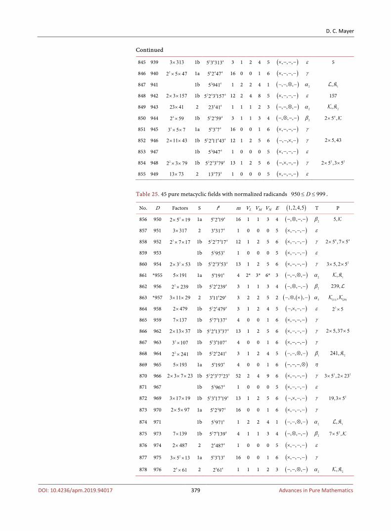
D. C. Mayer
DOI: 10.4236/apm.2019.94017 379 Advances in Pure Mathematics
Continued
845 939 3 313× 1b 2 4 45 3 313 3 1 2 4 5 ( ), , ,× − − − ε 5
846 940 22 5 47× × 1a 6 4 45 2 47 16 0 0 1 6 ( ), , ,× − − − γ
847 941 1b 2 45 941 1 2 2 4 1 ( ), , ,− − ⊗ − 2α 1,K
848 942 2 3 157× × 1b 2 4 4 45 2 3 157 12 2 4 8 5 ( ), , ,× − − − ε 157
849 943 23 41× 2 4 423 41 1 1 1 2 3 ( ), , ,− − ⊗ − 2α 2,K
850 944 42 59× 1b 2 4 45 2 59 3 1 1 3 4 ( ), , ,− ⊗ − − 2β 42 5 ,×
851 945 33 5 7× × 1a 6 4 45 3 7 16 0 0 1 6 ( ), , ,× − − − γ
852 946 2 11 43× × 1b 2 4 4 45 2 11 43 12 1 2 5 6 ( ), , ,− − × − γ 2 5,43×
853 947 1b 2 45 947 1 0 0 0 5 ( ), , ,× − − − ε
854 948 22 3 79× × 1b 2 4 4 45 2 3 79 13 1 2 5 6 ( ), , ,− × − − γ 2 22 5 ,3 5× ×
855 949 13 73× 2 4 413 73 1 0 0 0 5 ( ), , ,× − − − ε
Table 25. 45 pure metacyclic fields with normalized radicands 950 999D≤ ≤ .
No. D Factors S f4 m VL VM VN E ( )1,2,4,5 T P
856 950 22 5 19× × 1a 6 4 45 2 19 16 1 1 3 4 ( ), , ,− ⊗ − − 2β 5,
857 951 3 317× 2 4 43 317 1 0 0 0 5 ( ), , ,× − − − ε
858 952 32 7 17× × 1b 2 4 4 45 2 7 17 12 1 2 5 6 ( ), , ,× − − − γ 4 42 5 ,7 5× ×
859 953 1b 2 45 953 1 0 0 0 5 ( ), , ,× − − − ε
860 954 22 3 53× × 1b 2 4 4 45 2 3 53 13 1 2 5 6 ( ), , ,× − − − γ 23 5,2 5× ×
861 *955 5 191× 1a 6 45 191 4 2* 3* 6* 3 ( ), , ,− − ⊗ − 2α 1,K
862 956 22 239× 1b 2 4 45 2 239 3 1 1 3 4 ( ), , ,− ⊗ − − 2β 239,
863 *957 3 11 29× × 2 4 4 43 11 29 3 2 2 5 2 ( )( ), , ,− ⊗ × − 3α (11) (29),
864 958 2 479× 1b 2 4 45 2 479 3 1 2 4 5 ( ), , ,− × − − ε 32 5×
865 959 7 137× 1b 2 4 45 7 137 4 0 0 1 6 ( ), , ,× − − − γ
866 962 2 13 37× × 1b 2 4 4 45 2 13 37 13 1 2 5 6 ( ), , ,× − − − γ 2 5,37 5× ×
867 963 23 107× 1b 2 4 45 3 107 4 0 0 1 6 ( ), , ,× − − − γ
868 964 22 241× 1b 2 4 45 2 241 3 1 2 4 5 ( ), , ,− − ⊗ − 1β 2241,K
869 965 5 193× 1a 6 45 193 4 0 0 1 6 ( ), , ,− − − ⊗ η
870 966 2 3 7 23× × × 1b 2 4 4 4 45 2 3 7 23 52 2 4 9 6 ( ), , ,× − − − γ 3 23 5 ,2 23× ×
871 967 1b 2 45 967 1 0 0 0 5 ( ), , ,× − − − ε
872 969 3 17 19× × 1b 2 4 4 45 3 17 19 13 1 2 5 6 ( ), , ,− × − − γ 219,3 5×
873 970 2 5 97× × 1a 6 4 45 2 97 16 0 0 1 6 ( ), , ,× − − − γ
874 971 1b 2 45 971 1 2 2 4 1 ( ), , ,− − ⊗ − 2α 1,K
875 973 7 139× 1b 2 4 45 7 139 4 1 1 3 4 ( ), , ,− ⊗ − − 2β 27 5 ,×
876 974 2 487× 2 4 42 487 1 0 0 0 5 ( ), , ,× − − − ε
877 975 23 5 13× × 1a 6 4 45 3 13 16 0 0 1 6 ( ), , ,× − − − γ
878 976 42 61× 2 4 42 61 1 1 1 2 3 ( ), , ,− − ⊗ − 2α 2,K

D. C. Mayer
DOI: 10.4236/apm.2019.94017 380 Advances in Pure Mathematics
Continued
879 977 1b 2 45 977 1 0 0 0 5 ( ), , ,× − − − ε
880 978 2 3 163× × 1b 2 4 4 45 2 3 163 13 1 2 5 6 ( ), , ,× − − − γ 2 43 5 ,2 5× ×
881 979 11 89× 1b 2 4 45 11 89 3 2 3 7 4 ( )( ), , ,− ⊗ × − 2β 2(11) (89)11, ⋅
882 980 2 22 5 7× × 1a 6 4 45 2 7 16 1 2 4 5 ( ), , ,× − − − ε 7
883 981 23 109× 1b 2 4 45 3 109 3 1 1 3 4 ( ), , ,− ⊗ − − 2β 109,
884 *982 2 491× 2 4 42 491 1 1 1 2 3 ( ), , ,− − ⊗ − 2α 1,K
885 983 1b 2 45 983 1 0 0 0 5 ( ), , ,× − − − ε
886 984 32 3 41× × 1b 2 4 4 45 2 3 41 13 1 2 5 6 ( ), , ,− − × − γ 23, 2 5×
887 985 5 197× 1a 6 45 197 4 0 0 0 5 ( ), , ,× − − − ε
888 986 2 17 29× × 1b 2 4 4 45 2 17 29 13 2 4 8 5 ( ), , ,− × − − ε 2 5×
889 987 3 7 47× × 1b 2 4 4 45 3 7 47 12 1 2 5 6 ( ), , ,× − − − γ 2 47 5 ,3 5× ×
890 988 22 13 19× × 1b 2 4 4 45 2 13 19 13 1 2 5 6 ( ), , ,− × − − γ 22,13 5×
891 989 23 43× 1b 2 4 45 23 43 4 0 0 1 6 ( ), , ,× − − − γ
892 990 22 3 5 11× × × 1a 6 4 4 45 2 3 11 64 1 2 5 6 ( ), , ,− − × − γ 22 5,3 5× ×
893 991 1b 2 45 991 1 1 2 3 4 ( ), , ,− − ⊗ − 1δ 1K
894 993 3 331× 2 4 43 331 1 1 1 2 3 ( ), , ,− − ⊗ − 2α 2,K
895 994 2 7 71× × 1b 2 4 4 45 2 7 71 12 2 3 7 4 ( )( ), , ,− − × − 2β 32 5 ,×
896 995 5 199× 1a 6 45 199 4 1 1 3 4 ( ), , ,− ⊗ − ⊗ 2ζ
897 996 22 3 83× × 1b 2 4 4 45 2 3 83 13 1 2 5 6 ( ), , ,× − − − γ 2 42 5 ,3 5× ×
898 997 1b 2 45 997 1 0 0 0 5 ( ), , ,× − − − ε
899 998 2 499× 1b 2 4 45 2 499 4 1 1 3 4 ( ), , ,− ⊗ − − 2β 499,
900 999 33 37× 2 4 43 37 1 0 0 0 5 ( ), , ,× − − − ε
Table 26. Absolute frequencies of differential principal factorization types.
Type 100 200 300 400 500 600 700 800 900 1000 %
1α 1 2 3 4 5 5 5 9 9 9
2α 10 17 23 30 35 42 52 57 63 75 8.3
3α 0 0 0 1 1 3 5 5 7 8
1β 0 2 4 7 8 11 15 18 22 23
2β 7 24 40 54 80 94 108 126 146 161 17.9
γ 25 55 88 117 148 187 222 259 290 324 36.0
1δ 0 0 1 1 3 4 4 4 6 7
2δ 8 14 19 23 31 35 38 44 51 53 5.9
ε 26 45 67 95 110 128 150 165 184 208 23.4
1ζ 0 1 1 1 1 1 1 1 1 1
2ζ 0 0 0 0 0 1 1 4 4 5 η 1 2 4 5 5 6 6 6 6 7 ϑ 3 6 8 9 11 13 15 17 18 19
Total 81 168 258 347 438 530 622 715 807 900 100.0
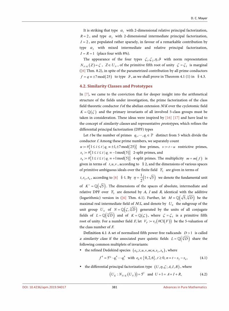
D. C. Mayer
DOI: 10.4236/apm.2019.94017 381 Advances in Pure Mathematics
It is striking that type 1α with 2-dimensional relative principal factorization, 2R = , and type 3α with 2-dimensional intermediate principal factorization, 2I = , are populated rather sparsely, in favour of a remarkable contribution by
type 2α with mixed intermediate and relative principal factorization, 1I R= = (place four with 8%).
The appearance of the four types 1 2, , ,ζ ζ η ϑ with norm representation ( )/N KN Z ζ= , NZ U∈ , of the primitive fifth root of unity 5ζ ζ= is marginal
([6] Thm. 8.2), in spite of the parametrized contribution by all prime conductors ( )7 mod 25f q= ≡ ± to type ϑ , as we shall prove in Theorem 4.1 (1) in §4.3.
4.2. Similarity Classes and Prototypes
In [7], we came to the conviction that for deeper insight into the arithmetical structure of the fields under investigation, the prime factorization of the class field theoretic conductor f of the abelian extension N/K over the cyclotomic field
( )K ζ= and the primary invariants of all involved 5-class groups must be taken in consideration. These ideas were inspired by [16] [17] and have lead to the concept of similarity classes and representative prototypes, which refines the differential principal factorization (DPF) types
Let t be the number of primes 1, , tq q ∈ distinct from 5 which divide the conductor f. Among these prime numbers, we separately count
( ){ }: # 1 | 1, 7 mod 25iu i t q= ≤ ≤ ≡ ± ± free primes, :v t u= − restrictive primes, ( ){ }2 : # 1 | 1mod 5is i t q= ≤ ≤ ≡ − 2-split primes, and ( ){ }4 : # 1 | 1mod 5is i t q= ≤ ≤ ≡ + 4-split primes. The multiplicity ( )m m f= is
given in terms of , ,t u v , according to §2, and the dimensions of various spaces of primitive ambiguous ideals over the finite field 5 are given in terms of
2 4, ,t s s , according to [6] §4. By ( )1 1 52
η = + we denote the fundamental unit
of ( )5K + = . The dimensions of the spaces of absolute, intermediate and relative DPF over 5 are denoted by A, I and R, identical with the additive (logarithmic) version in ([6] Thm. 6.1). Further, let ( )55,M D= be the maximal real intermediate field of N/L, and denote by 0U the subgroup of the unit group NU of ( )5,N Dζ= generated by the units of all conjugate fields of ( )5L D= and of ( )K ζ= , where 5ζ ζ= is a primitive fifth root of unity. For a number field F, let ( )( )5: #ClFV v F= be the 5-valuation of the class number of F.
Definition 4.1 A set of normalized fifth power free radicands 1D > is called a similarity class if the associated pure quintic fields ( )5L D= share the following common multiplets of invariants: the refined Dedekind species ( )0 2 4; , , , ; , ,e t u v m n s s , where
{ }04 4 41 0 2 45 with 0,2,6 , 0, ,e
tf q q e t n t s s= ⋅ ∈ ≥ = − − (4.1)
the differential principal factorization type ( ), , ; , ,U A I Rη ζ , where
( )( )/: 5 and 1 ,UK N K NU N U U A I R= + = + + (4.2)
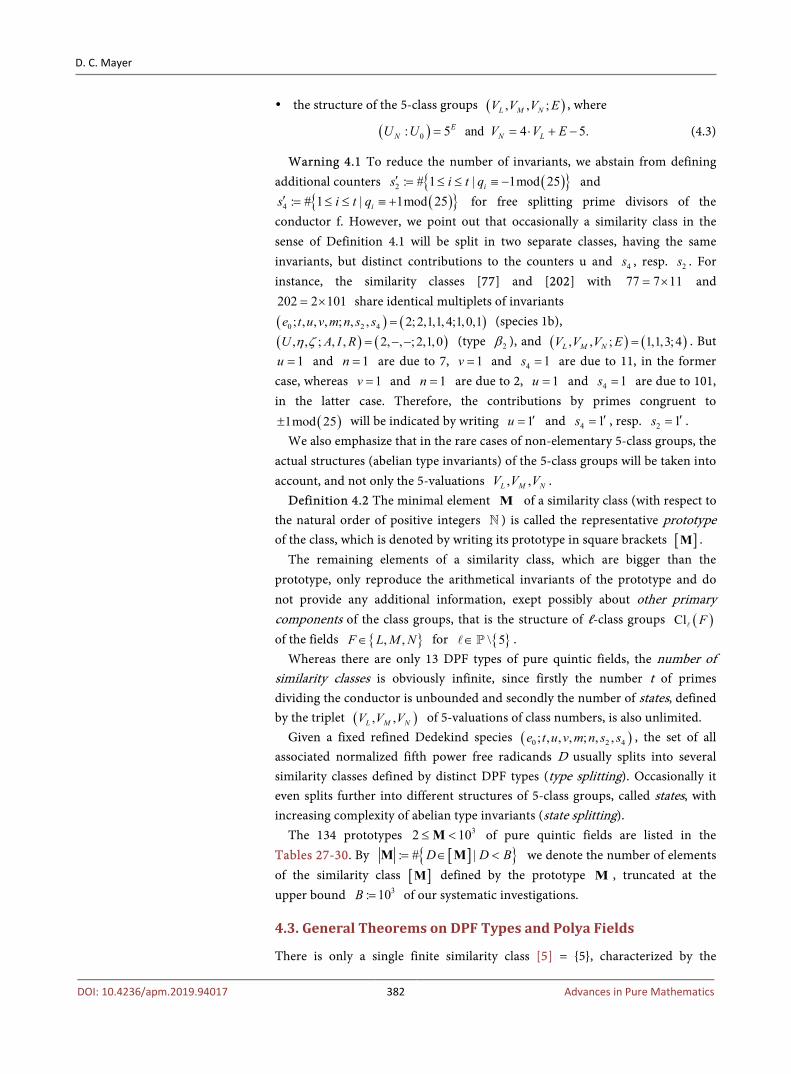
D. C. Mayer
DOI: 10.4236/apm.2019.94017 382 Advances in Pure Mathematics
the structure of the 5-class groups ( ), , ;L M NV V V E , where
( )0: 5 and 4 5.EN N LU U V V E= = ⋅ + − (4.3)
Warning 4.1 To reduce the number of invariants, we abstain from defining additional counters ( ){ }2 : # 1 | 1mod 25is i t q′ = ≤ ≤ ≡ − and
( ){ }4 : # 1 | 1mod 25is i t q′ = ≤ ≤ ≡ + for free splitting prime divisors of the conductor f. However, we point out that occasionally a similarity class in the sense of Definition 4.1 will be split in two separate classes, having the same invariants, but distinct contributions to the counters u and 4s , resp. 2s . For instance, the similarity classes [77] and [202] with 77 7 11= × and 202 2 101= × share identical multiplets of invariants ( ) ( )0 2 4; , , , ; , , 2;2,1,1, 4;1,0,1e t u v m n s s = (species 1b), ( ) ( ), , ; , , 2, , ;2,1,0U A I Rη ζ = − − (type 2β ), and ( ) ( ), , ; 1,1,3;4L M NV V V E = . But
1u = and 1n = are due to 7, 1v = and 4 1s = are due to 11, in the former case, whereas 1v = and 1n = are due to 2, 1u = and 4 1s = are due to 101, in the latter case. Therefore, the contributions by primes congruent to
( )1mod 25± will be indicated by writing 1u ′= and 4 1s ′= , resp. 2 1s ′= . We also emphasize that in the rare cases of non-elementary 5-class groups, the
actual structures (abelian type invariants) of the 5-class groups will be taken into account, and not only the 5-valuations , ,L M NV V V .
Definition 4.2 The minimal element M of a similarity class (with respect to the natural order of positive integers ) is called the representative prototype of the class, which is denoted by writing its prototype in square brackets [ ]M .
The remaining elements of a similarity class, which are bigger than the prototype, only reproduce the arithmetical invariants of the prototype and do not provide any additional information, exept possibly about other primary components of the class groups, that is the structure of ℓ-class groups ( )Cl F
of the fields { }, ,F L M N∈ for { }\ 5∈ .
Whereas there are only 13 DPF types of pure quintic fields, the number of similarity classes is obviously infinite, since firstly the number t of primes dividing the conductor is unbounded and secondly the number of states, defined by the triplet ( ), ,L M NV V V of 5-valuations of class numbers, is also unlimited.
Given a fixed refined Dedekind species ( )0 2 4; , , , ; , ,e t u v m n s s , the set of all associated normalized fifth power free radicands D usually splits into several similarity classes defined by distinct DPF types (type splitting). Occasionally it even splits further into different structures of 5-class groups, called states, with increasing complexity of abelian type invariants (state splitting).
The 134 prototypes 32 10≤ <M of pure quintic fields are listed in the Tables 27-30. By [ ]{ }: # |D D B= ∈ <M M we denote the number of elements of the similarity class [ ]M defined by the prototype M , truncated at the upper bound 3: 10B = of our systematic investigations.
4.3. General Theorems on DPF Types and Polya Fields
There is only a single finite similarity class [5] = {5}, characterized by the
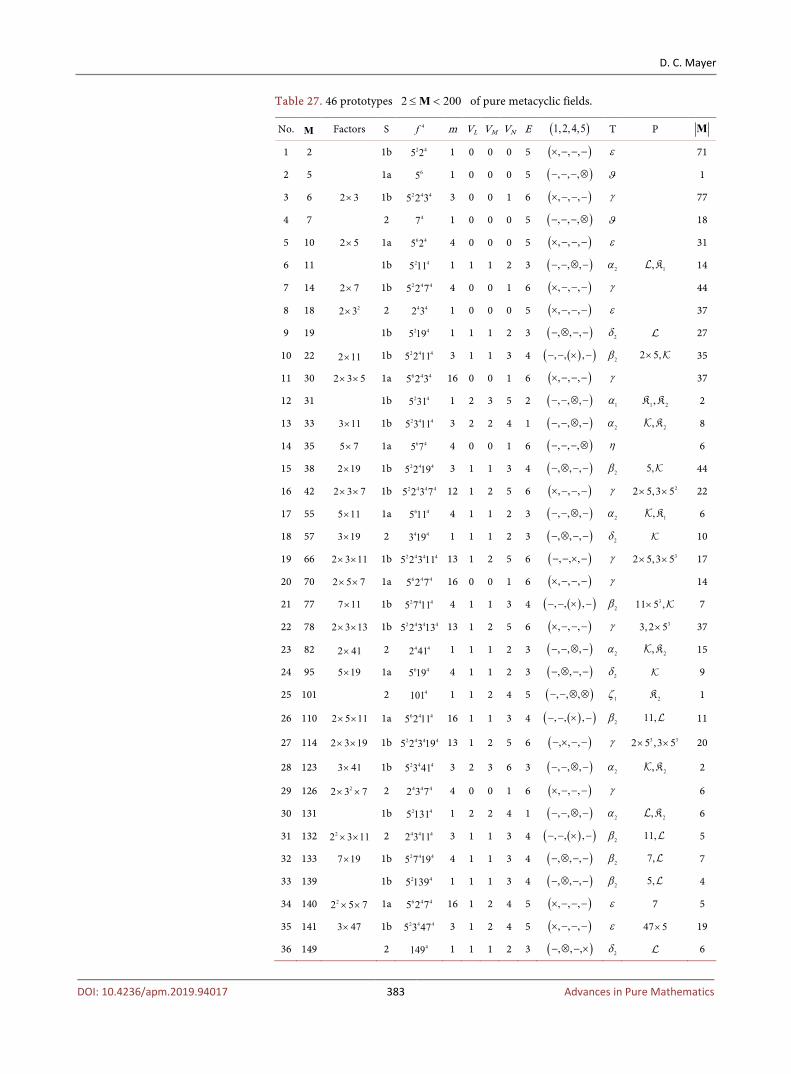
D. C. Mayer
DOI: 10.4236/apm.2019.94017 383 Advances in Pure Mathematics
Table 27. 46 prototypes 2 200≤ <M of pure metacyclic fields.
No. M Factors S 4f m VL VM VN E ( )1,2,4,5 T P M
1 2 1b 2 45 2 1 0 0 0 5 ( ), , ,× − − − ε 71
2 5 1a 65 1 0 0 0 5 ( ), , ,− − − ⊗ ϑ 1
3 6 2 3× 1b 2 4 45 2 3 3 0 0 1 6 ( ), , ,× − − − γ 77
4 7 2 47 1 0 0 0 5 ( ), , ,− − − ⊗ ϑ 18
5 10 2 5× 1a 6 45 2 4 0 0 0 5 ( ), , ,× − − − ε 31
6 11 1b 2 45 11 1 1 1 2 3 ( ), , ,− − ⊗ − 2α 1,K 14
7 14 2 7× 1b 2 4 45 2 7 4 0 0 1 6 ( ), , ,× − − − γ 44
8 18 22 3× 2 4 42 3 1 0 0 0 5 ( ), , ,× − − − ε 37
9 19 1b 2 45 19 1 1 1 2 3 ( ), , ,− ⊗ − − 2δ 27
10 22 2 11× 1b 2 4 45 2 11 3 1 1 3 4 ( )( ), , ,− − × − 2β 2 5,× 35
11 30 2 3 5× × 1a 6 4 45 2 3 16 0 0 1 6 ( ), , ,× − − − γ 37
12 31 1b 2 45 31 1 2 3 5 2 ( ), , ,− − ⊗ − 1α 1 2,K K 2
13 33 3 11× 1b 2 4 45 3 11 3 2 2 4 1 ( ), , ,− − ⊗ − 2α 2,K 8
14 35 5 7× 1a 6 45 7 4 0 0 1 6 ( ), , ,− − − ⊗ η 6
15 38 2 19× 1b 2 4 45 2 19 3 1 1 3 4 ( ), , ,− ⊗ − − 2β 5, 44
16 42 2 3 7× × 1b 2 4 4 45 2 3 7 12 1 2 5 6 ( ), , ,× − − − γ 22 5,3 5× × 22
17 55 5 11× 1a 6 45 11 4 1 1 2 3 ( ), , ,− − ⊗ − 2α 1,K 6
18 57 3 19× 2 4 43 19 1 1 1 2 3 ( ), , ,− ⊗ − − 2δ 10
19 66 2 3 11× × 1b 2 4 4 45 2 3 11 13 1 2 5 6 ( ), , ,− − × − γ 32 5,3 5× × 17
20 70 2 5 7× × 1a 6 4 45 2 7 16 0 0 1 6 ( ), , ,× − − − γ 14
21 77 7 11× 1b 2 4 45 7 11 4 1 1 3 4 ( )( ), , ,− − × − 2β 311 5 ,× 7
22 78 2 3 13× × 1b 2 4 4 45 2 3 13 13 1 2 5 6 ( ), , ,× − − − γ 33, 2 5× 37
23 82 2 41× 2 4 42 41 1 1 1 2 3 ( ), , ,− − ⊗ − 2α 2,K 15
24 95 5 19× 1a 6 45 19 4 1 1 2 3 ( ), , ,− ⊗ − − 2δ 9
25 101 2 4101 1 1 2 4 5 ( ), , ,− − ⊗ ⊗ 1ζ 2K 1
26 110 2 5 11× × 1a 6 4 45 2 11 16 1 1 3 4 ( )( ), , ,− − × − 2β 11, 11
27 114 2 3 19× × 1b 2 4 4 45 2 3 19 13 1 2 5 6 ( ), , ,− × − − γ 3 32 5 ,3 5× × 20
28 123 3 41× 1b 2 4 45 3 41 3 2 3 6 3 ( ), , ,− − ⊗ − 2α 2,K 2
29 126 22 3 7× × 2 4 4 42 3 7 4 0 0 1 6 ( ), , ,× − − − γ 6
30 131 1b 2 45 131 1 2 2 4 1 ( ), , ,− − ⊗ − 2α 2,K 6
31 132 22 3 11× × 2 4 4 42 3 11 3 1 1 3 4 ( )( ), , ,− − × − 2β 11, 5
32 133 7 19× 1b 2 4 45 7 19 4 1 1 3 4 ( ), , ,− ⊗ − − 2β 7, 7
33 139 1b 2 45 139 1 1 1 3 4 ( ), , ,− ⊗ − − 2β 5, 4
34 140 22 5 7× × 1a 6 4 45 2 7 16 1 2 4 5 ( ), , ,× − − − ε 7 5
35 141 3 47× 1b 2 4 45 3 47 3 1 2 4 5 ( ), , ,× − − − ε 47 5× 19
36 149 2 4149 1 1 1 2 3 ( ), , ,− ⊗ − × 2δ 6

D. C. Mayer
DOI: 10.4236/apm.2019.94017 384 Advances in Pure Mathematics
Continued
37 151 2 4151 1 1 1 2 3 ( ), , ,− − ⊗ × 2α 1,K 3
38 154 2 7 11× × 1b 2 4 4 45 2 7 11 12 2 3 7 4 ( )( ), , ,− − × − 2β 22 11 ,× 3
39 155 5 31× 1a 6 45 31 4 2 3 5 2 ( ), , ,− − ⊗ − 1α 1 2,K K 2
40 171 23 19× 1b 2 4 45 3 19 3 1 2 4 5 ( ), , ,− × − − ε 219 5× 6
41 174 2 3 29× × 2 4 4 42 3 29 3 1 1 3 4 ( ), , ,− ⊗ − − 2β 23 29,× 3
42 180 2 22 3 5× × 1a 6 4 45 2 3 16 1 2 4 5 ( ), , ,× − − − ε 3 5
43 182 2 7 13× × 2 4 4 42 7 13 4 1 2 4 5 ( ), , ,× − − − ε 7 1
44 186 2 3 31× × 1b 2 4 4 45 2 3 31 13 2 3 6 3 ( ), , ,− − ⊗ − 1β 25,K 7
45 190 2 5 19× × 1a 6 4 45 2 19 16 1 1 3 4 ( ), , ,− ⊗ − − 2β 5, 9
46 191 1b 2 45 191 1 1 2 4 5 ( ), , ,− − ⊗ − 1β 15,K 3
Table 28. 44 prototypes 200 510< <M of pure metacyclic fields.
No. M Factors S 4f m VL VM VN E ( )1,2,4,5 T P M
47 202 2 101× 1b 2 4 45 2 101 4 1 1 3 4 ( ), , ,− ⊗ − − 2β 2 5,× 6
48 203 7 29× 1b 2 4 45 7 29 4 1 2 4 5 ( ), , ,− × − − ε 29 5× 2
49 209 11 19× 1b 2 4 45 11 19 3 2 3 7 4 ( ), , ,− ⊗ × − 2β ( )2
1911 5 ,× 2
50 210 2 3 5 7× × × 1a 6 4 4 45 2 3 7 64 1 2 5 6 ( ), , ,× − − − γ 27,3 5× 5
51 211 1b 2 45 211 1 3 5 9 2 ( ), , ,− − ⊗ − 1δ 2K 1
52 218 2 109× 2 4 42 109 1 1 2 4 5 ( ), , ,− × − − ε 2 1
53 231 3 7 11× × 1b 2 4 4 45 3 7 11 12 1 2 5 6 ( ), , ,− − × − γ 211,7 5× 5
54 247 13 19× 1b 2 4 45 13 19 3 1 2 5 6 ( ), , ,− × − − γ 2
55 253 11 23× 1b 2 4 45 11 23 3 1 2 4 5 ( ), , ,− − ⊗ − 1β 111,K 4
56 259 7 37× 1b 2 4 45 7 37 4 1 2 5* 6 ( ), , ,× − − − γ 1
57 266 2 7 19× × 1b 2 4 4 45 2 7 19 12 1 2 5 6 ( ), , ,− × − − γ 35, 2 7× 3
58 273 3 7 13× × 1b 2 4 4 45 3 7 13 12 2 4 8 5 ( ), , ,× − − − ε 2 47 13 5× × 4
59 275 25 11× 1a 6 45 11 4 2 2 4 1 ( ), , ,− − ⊗ − 2α 2,K 2
60 276 22 3 23× × 2 4 4 42 3 23 3 0 0 1 6 ( ), , ,× − − − γ 10
61 281 1b 2 45 281 1 3 5* 9* 2 ( ), , ,− − ⊗ − 1α 1 2,K K 1
62 285 3 5 19× × 1a 6 4 45 3 19 16 1 2 5 6 ( ), , ,− × − − γ 1
63 286 2 11 13× × 1b 2 4 4 45 2 11 13 13 2 3 7 4 ( )( ), , ,− − × − 2β 211 5,× 3
64 287 7 41× 1b 2 4 45 7 41 4 2 2 4 1 ( ), , ,− − ⊗ − 2α 1,K 1
65 290 2 5 29× × 1a 6 4 45 2 29 16 1 2 4 5 ( ), , ,− × − − ε 29 2
66 298 2 149× 1b 2 4 45 2 149 4 1 2 4 5 ( ), , ,− × − − ε 5 2
67 301 7 43× 2 4 47 43 4 0 0 1 6 ( ), , ,− − − ⊗ η 1
68 302 2 151× 1b 2 4 45 2 151 4 1 2 4 5 ( ), , ,− − ⊗ − 1β 12,K 2
69 319 11 29× 1b 2 4 45 11 29 3 2 2 5 2 ( )( ), , ,− ⊗ × − 3α ( ) ( )11 29, 3
70 329 7 47× 1b 2 4 45 7 47 4 1 2 4 5 ( ), , ,× − − − ε 47 7
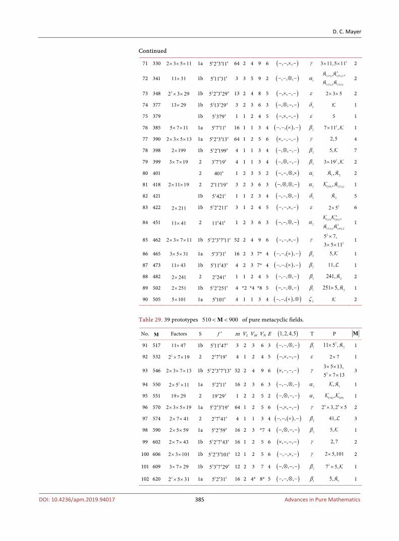
D. C. Mayer
DOI: 10.4236/apm.2019.94017 385 Advances in Pure Mathematics
Continued
71 330 2 3 5 11× × × 1a 6 4 4 45 2 3 11 64 2 4 9 6 ( ), , ,− − × − γ 33 11,5 11× × 2
72 341 11 31× 1b 2 4 45 11 31 3 3 5 9 2 ( ), , ,− − ⊗ − 1α 3
(11),1 (31),2
(11),2 (31),1
,K K
K K 2
73 348 22 3 29× × 1b 2 4 4 45 2 3 29 13 2 4 8 5 ( ), , ,− × − − ε 2 3 5× × 2
74 377 13 29× 1b 2 4 45 13 29 3 2 3 6 3 ( ), , ,− ⊗ − − 2δ 1
75 379 1b 2 45 379 1 1 2 4 5 ( ), , ,− × − − ε 5 1
76 385 5 7 11× × 1a 6 4 45 7 11 16 1 1 3 4 ( )( ), , ,− − × − 2β 27 11 ,× 1
77 390 2 3 5 13× × × 1a 6 4 4 45 2 3 13 64 1 2 5 6 ( ), , ,× − − − γ 2,5 4
78 398 2 199× 1b 2 4 45 2 199 4 1 1 3 4 ( ), , ,− ⊗ − − 2β 5, 7
79 399 3 7 19× × 2 4 4 43 7 19 4 1 1 3 4 ( ), , ,− ⊗ − − 2β 23 19 ,× 2
80 401 2 4401 1 2 3 5 2 ( ), , ,− − ⊗ × 1α 1 2,K K 2
81 418 2 11 19× × 2 4 4 42 11 19 3 2 3 6 3 ( ), , ,− ⊗ ⊗ − 2α (19) (11),1,K 1
82 421 1b 2 45 421 1 1 2 3 4 ( ), , ,− − ⊗ − 1δ 2K 5
83 422 2 211× 1b 2 4 45 2 211 3 1 2 4 5 ( ), , ,− − × − ε 22 5× 6
84 451 11 41× 2 4 411 41 1 2 3 6 3 ( ), , ,− − ⊗ − 2α 4
(11) (41)
3(11),1 (41),2
,
K K 1
85 462 2 3 7 11× × × 1b 2 4 4 4 45 2 3 7 11 52 2 4 9 6 ( ), , ,− − × − γ 2
2
5 7,3 5 11×
× × 1
86 465 3 5 31× × 1a 6 4 45 3 31 16 2 3 7* 4 ( )( ), , ,− − × − 2β 5, 1
87 473 11 43× 1b 2 4 45 11 43 4 2 3 7* 4 ( )( ), , ,− − × − 2β 11, 1
88 482 2 241× 2 4 42 241 1 1 2 4 5 ( ), , ,− − ⊗ − 1β 2241,K 2
89 502 2 251× 1b 2 4 45 2 251 4 *2 *4 *8 5 ( ), , ,− − ⊗ − 1β 2251 5,× K 1
90 505 5 101× 1a 6 45 101 4 1 1 3 4 ( )( ), , ,− − × ⊗ 2ζ 2
Table 29. 39 prototypes 510 900< <M of pure metacyclic fields.
No. M Factors S 4f m VL VM VN E ( )1,2,4,5 T P M
91 517 11 47× 1b 2 4 45 11 47 3 2 3 6 3 ( ), , ,− − ⊗ − 1β 2211 5 ,× K 1
92 532 22 7 19× × 2 4 4 42 7 19 4 1 2 4 5 ( ), , ,− × − − ε 2 7× 1
93 546 2 3 7 13× × × 1b 2 4 4 4 45 2 3 7 13 52 2 4 9 6 ( ), , ,× − − − γ 2
3 5 13,5 7 13× ×
× × 3
94 550 22 5 11× × 1a 6 4 45 2 11 16 2 3 6 3 ( ), , ,− − ⊗ − 2α 1,K 1
95 551 19 29× 2 4 419 29 1 2 2 5 2 ( ), , ,− ⊗ − − 3α (19) (29), 1
96 570 2 3 5 19× × × 1a 6 4 4 45 2 3 19 64 1 2 5 6 ( ), , ,− × − − γ 4 42 3,2 5× × 2
97 574 2 7 41× × 2 4 4 42 7 41 4 1 1 3 4 ( )( ), , ,− − × − 2β 41, 3
98 590 2 5 59× × 1a 6 4 45 2 59 16 2 3 *7 4 ( ), , ,− ⊗ − − 2β 5, 1
99 602 2 7 43× × 1b 2 4 4 45 2 7 43 16 1 2 5 6 ( ), , ,× − − − γ 2,7 2
100 606 2 3 101× × 1b 2 4 4 45 2 3 101 12 1 2 5 6 ( ), , ,− − × − γ 2 5,101× 2
101 609 3 7 29× × 1b 2 4 4 45 3 7 29 12 2 3 7 4 ( ), , ,− ⊗ − − 2β 27 5,× 1
102 620 22 5 31× × 1a 6 4 45 2 31 16 2 4* 8* 5 ( ), , ,− − ⊗ − 1β 15,K 1

D. C. Mayer
DOI: 10.4236/apm.2019.94017 386 Advances in Pure Mathematics
Continued
103 627 3 11 19× × 1b 2 4 4 45 3 11 19 13 3 4 9 2 ( )( ), , ,− ⊗ × − 3α (11) (19), 1
104 638 2 11 29× × 1b 2 4 4 45 2 11 29 13 2 3 7 4 ( )( ), , ,− ⊗ × − 2β 4
4(11) (29)
2 11 5,× ×
× 2
105 649 11 59× 2 4 411 59 1 2 2 5 2 ( )( ), , ,− ⊗ × − 3α (11) (59), 2
106 660 22 3 5 11× × × 1a 6 4 4 45 2 3 11 64 1 2 5 6 ( ), , ,− − × − γ 2 5,5 11× × 2
107 665 5 7 19× × 1a 6 4 45 7 19 16 1 1 3 4 ( ), , ,− ⊗ − − 2β 7, 1
108 671 11 61× 1b 2 4 45 11 61 3 3 4 8 1 ( ), , ,− − ⊗ − 2α (11) (61)
2(11),2 (61),1
,
K K 1
109 682 2 11 31× × 2 4 4 42 11 31 3 2 3 6 3 ( ), , ,− − ⊗ − 2α 3
(11) (31)
3(11),1 (31),2
,
K K 1
110 691 1b 2 45 691 1 3 4 8 1 ( ), , ,− − ⊗ − 2α 2,K 1
111 693 23 7 11× × 2 4 4 43 7 11 4 2 3 6 3 ( ), , ,− − ⊗ − 1β 23 7,× K 1
112 695 5 139× 1a 6 45 139 4 1 2 4 5 ( ), , ,− × − − ε 139 1
113 702 32 3 13× × 1b 2 4 4 45 2 3 13 13 2 4 8 5 ( ), , ,× − − − ε 413 5× 2
114 707 7 101× 2 4 47 101 4 1 1 3 4 ( )( ), , ,− − × ⊗ 2ζ 1
115 710 2 5 71× × 1a 6 4 45 2 71 16 2 2 4 1 ( ), , ,− − ⊗ − 2α 2,K 4
116 745 5 149× 1a 6 45 149 4 1 1 3 4 ( ), , ,− ⊗ − ⊗ 2ζ 2
117 749 7 107× 2 4 47 107 4 1 2 4 5 ( ), , ,− − − × ε 1
118 751 2 4751 1 2 2 4 1 ( ), , ,− − ⊗ × 2α 1,K 1
119 770 2 5 7 11× × × 1a 6 4 4 45 2 7 11 64 1 2 5 6 ( ), , ,− − × − γ 22 5,2 11× × 1
120 779 19 41× 1b 2 4 45 19 41 3 3 4 8 1 ( ), , ,− ⊗ ⊗ − 2α (19) (41)
(41),1
,
K 1
121 785 5 157× 1a 6 45 157 4 1 2 4 5 ( ), , ,− − − × ε 1
122 798 2 3 7 19× × ⋅ 1b 2 4 4 4 45 2 3 7 19 52 2 4 9 6 ( ), , ,− × − − γ 43 19,7 5× × 1
123 808 32 101× 1b 2 4 45 2 101 4 2 2 4 1 ( ), , ,− − ⊗ − 2α 1,K 2
124 825 23 5 11× × 1a 6 4 45 3 11 16 1 2 4 5 ( ), , ,− − ⊗ − 1β 213 11,× K 1
125 843 3 281× 2 4 43 281 1 1 2 3 4 ( ), , ,− − ⊗ − 1δ 1K 1
126 858 2 3 11 13× × × 1b 2 4 4 4 45 2 3 11 13 51 2 4 9 6 ( ), , ,− − × − γ 2 5,13 5× × 1
127 861 3 7 41× × 1b 2 4 4 45 3 7 41 13 3 4 8 1 ( ), , ,− − ⊗ − 2α 1,K 1
128 893 19 47× 2 4 419 47 1 1 1 3 4 ( ), , ,− ⊗ − − 2β 19,L 1
129 894 2 3 149× × 1b 2 4 4 45 2 3 149 12 1 2 5 6 ( ), , ,− × − − γ 25, 2 3× 1
exceptional number 0t = of primes 5q ≠ dividing the conductor f (here
4 65f = ). The invariants of this unique metacyclic Polya field N are given by
[5], species 1a, ( ) ( )0 2 4; , , , ; , , 6;0,0,0,1;0,0,0e t u v m n s s = ,
type ϑ , ( ) ( ), , ; , , 0, , ;1,0,0U A I Rη ζ = × × , and ( ) ( ), , ; 0,0,0;5L M NV V V E = . (4.4) We conjecture that all the other similarity classes are infinite. Precisely four of
them can actually be given by parametrized infinite sequences in a deterministic way aside from the intrinsic probabilistic nature of the occurrence of primes in
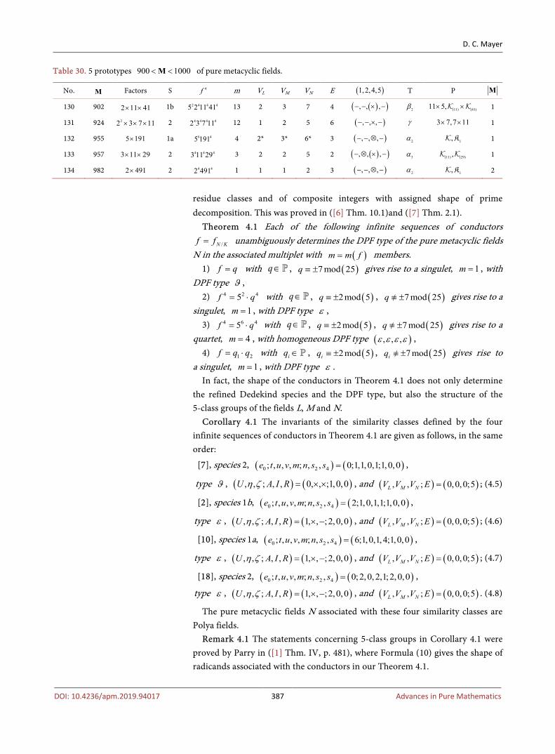
D. C. Mayer
DOI: 10.4236/apm.2019.94017 387 Advances in Pure Mathematics
Table 30. 5 prototypes 900 1000< <M of pure metacyclic fields.
No. M Factors S 4f m VL VM VN E ( )1,2,4,5 T P M
130 902 2 11 41× × 1b 2 4 4 45 2 11 41 13 2 3 7 4 ( )( ), , ,− − × − 2β (11) (41)11 5,× × 1
131 924 22 3 7 11× × × 2 4 4 4 42 3 7 11 12 1 2 5 6 ( ), , ,− − × − γ 3 7,7 11× × 1
132 955 5 191× 1a 6 45 191 4 2* 3* 6* 3 ( ), , ,− − ⊗ − 2α 1,K 1
133 957 3 11 29× × 2 4 4 43 11 29 3 2 2 5 2 ( )( ), , ,− ⊗ × − 3α (11) (29), 1
134 982 2 491× 2 4 42 491 1 1 1 2 3 ( ), , ,− − ⊗ − 2α 1,K 2
residue classes and of composite integers with assigned shape of prime decomposition. This was proved in ([6] Thm. 10.1)and ([7] Thm. 2.1).
Theorem 4.1 Each of the following infinite sequences of conductors
/N Kf f= unambiguously determines the DPF type of the pure metacyclic fields N in the associated multiplet with ( )m m f= members.
1) f q= with q∈ , ( )7 mod 25q ≡ ± gives rise to a singulet, 1m = , with DPF type ϑ ,
2) 4 2 45f q= ⋅ with q∈ , ( )2 mod 5q ≡ ± , ( )7 mod 25q ≡ ±/ gives rise to a singulet, 1m = , with DPF type ε ,
3) 4 6 45f q= ⋅ with q∈ , ( )2 mod 5q ≡ ± , ( )7 mod 25q ≡ ±/ gives rise to a quartet, 4m = , with homogeneous DPF type ( ), , ,ε ε ε ε ,
4) 1 2f q q= ⋅ with iq ∈ , ( )2mod 5iq ≡ ± , ( )7 mod 25iq ≡ ±/ gives rise to a singulet, 1m = , with DPF type ε .
In fact, the shape of the conductors in Theorem 4.1 does not only determine the refined Dedekind species and the DPF type, but also the structure of the 5-class groups of the fields L, M and N.
Corollary 4.1 The invariants of the similarity classes defined by the four infinite sequences of conductors in Theorem 4.1 are given as follows, in the same order:
[7], species 2, ( ) ( )0 2 4; , , , ; , , 0;1,1,0,1;1,0,0e t u v m n s s = ,
type ϑ , ( ) ( ), , ; , , 0, , ;1,0,0U A I Rη ζ = × × , and ( ) ( ), , ; 0,0,0;5L M NV V V E = ; (4.5)
[2], species 1b, ( ) ( )0 2 4; , , , ; , , 2;1,0,1,1;1,0,0e t u v m n s s = ,
type ε , ( ) ( ), , ; , , 1, , ;2,0,0U A I Rη ζ = × − , and ( ) ( ), , ; 0,0,0;5L M NV V V E = ; (4.6)
[10], species 1a, ( ) ( )0 2 4; , , , ; , , 6;1,0,1, 4;1,0,0e t u v m n s s = ,
type ε , ( ) ( ), , ; , , 1, , ;2,0,0U A I Rη ζ = × − , and ( ) ( ), , ; 0,0,0;5L M NV V V E = ; (4.7)
[18], species 2, ( ) ( )0 2 4; , , , ; , , 0;2,0, 2,1;2,0,0e t u v m n s s = ,
type ε , ( ) ( ), , ; , , 1, , ;2,0,0U A I Rη ζ = × − , and ( ) ( ), , ; 0,0,0;5L M NV V V E = . (4.8)
The pure metacyclic fields N associated with these four similarity classes are Polya fields.
Remark 4.1 The statements concerning 5-class groups in Corollary 4.1 were proved by Parry in ([1] Thm. IV, p. 481), where Formula (10) gives the shape of radicands associated with the conductors in our Theorem 4.1.
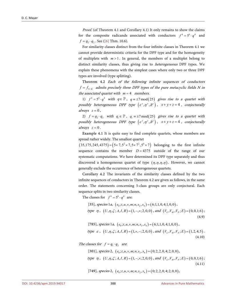
D. C. Mayer
DOI: 10.4236/apm.2019.94017 388 Advances in Pure Mathematics
Proof. (of Theorem 4.1 and Corollary 4.1) It only remains to show the claims for the composite radicands associated with conductors 4 6 45f q= ⋅ and
2 2f q q= ⋅ . See ([6] Thm. 10.6). For similarity classes distinct from the four infinite classes in Theorem 4.1 we
cannot provide deterministic criteria for the DPF type and for the homogeneity of multiplets with 1m > . In general, the members of a multiplet belong to distinct similarity classes, thus giving rise to heterogeneous DPF types. We explain these phenomena with the simplest cases where only two or three DPF types are involved (type splitting).
Theorem 4.2 Each of the following infinite sequences of conductors
/N Kf f= admits precisely three DPF types of the pure metacyclic fields N in the associated quartet with 4m = members.
1) 4 6 45f q= ⋅ with q∈ , ( )7 mod 25q ≡ ± gives rise to a quartet with possibly heterogeneous DPF type ( ), ,x y zε η ϑ , 4x y z+ + = , conjecturally always 0z = ,
2) 2 2f q q= ⋅ with iq ∈ , ( )7 mod 25iq ≡ ± gives rise to a quartet with possibly heterogeneous DPF type ( ), ,x y zε η ϑ , 4x y z+ + = , conjecturally always 0z = .
Example 4.1 It is quite easy to find complete quartets, whose members are spread rather widely. The smallest quartet ( ) ( )2 2 435,175,245,4375 5 7,5 7,5 7 ,5 7= × × × × belonging to the first infinite sequence contains the member 4375D = outside of the range of our systematic computations. We have determined its DPF type separately and thus discovered a homogeneous quartet of type ( ), , ,η η η η . However, we cannot generally exclude the occurrence of heterogeneous quartets.
Corollary 4.2 The invariants of the similarity classes defined by the two infinite sequences of conductors in Theorem 4.2 are given as follows, in the same order. The statements concerning 5-class groups are only conjectural. Each sequence splits in two similarity classes.
The classes for 4 6 45f q= ⋅ are:
[35], species 1a, ( ) ( )0 2 4; , , , ; , , 6;1,1,0,4;1,0,0e t u v m n s s = ,
type η , ( ) ( ) , , ; , , 1, , ;2,0,0U A I Rη ζ = − × , and ( ) ( ), , ; 0,0,1;6L M NV V V E = ; (4.9)
[785], species 1a, ( ) ( )0 2 4; , , , ; , , 6;1,1,0,4;1,0,0e t u v m n s s = ,
type ε , ( ) ( ) , , ; , , 1, , ;2,0,0U A I Rη ζ = × − , and ( ) ( ), , ; 1, 2, 4;5L M NV V V E = . (4.10)
The classes for 1 2f q q= ⋅ are:
[301], species 2, ( ) ( )0 2 4; , , , ; , , 0;2, 2,0, 4;2,0,0e t u v m n s s = ,
type η , ( ) ( ) , , ; , , 1, , ;2,0,0U A I Rη ζ = − × , and ( ) ( ), , ; 0,0,1;6L M NV V V E = ; (4.11)
[749], species 2, ( ) ( )0 2 4; , , , ; , , 0;2, 2,0, 4;2,0,0e t u v m n s s = ,
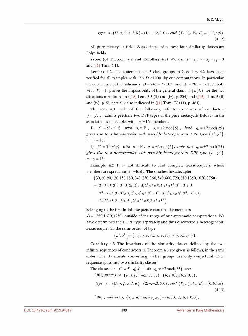
D. C. Mayer
DOI: 10.4236/apm.2019.94017 389 Advances in Pure Mathematics
type ε , ( ) ( ) , , ; , , 1, , ;2,0,0U A I Rη ζ = × − , and ( ) ( ), , ; 1, 2, 4;5L M NV V V E = . (4.12)
All pure metacyclic fields N associated with these four similarity classes are Polya fields.
Proof. (of Theorem 4.2 and Corollary 4.2) We use 2T = , 2 4 0v s s= = = and ([6] Thm. 6.1).
Remark 4.2. The statements on 5-class groups in Corollary 4.2 have been verified for all examples with 2 1000D≤ < by our computations. In particular, the occurrence of the radicands 749 7 107D = = × and 785 5 157D = = × , both with 1LV = , proves the impossibility of the general claim ( )5 h L for the two situations mentioned in ([18] Lem. 3.3 (ii) and (iv), p. 204) and ([15] Thm. 5 (ii) and (iv), p. 5), partially also indicated in ([1] Thm. IV (11), p. 481).
Theorem 4.3 Each of the following infinite sequences of conductors
/N Kf f= admits precisely two DPF types of the pure metacyclic fields N in the associated hexadecuplet with 16m = members.
1) 4 6 4 41 25f q q= ⋅ with iq ∈ , ( )2mod 5iq ≡ ± , both ( )7 mod 25iq ≡ ±/
gives rise to a hexadecuplet with possibly heterogeneous DPF type ( ),x yε γ , 16x y+ = ,
2) 4 6 4 41 25f q q= ⋅ with iq ∈ , ( )2mod 5iq ≡ ± , only one ( )7 mod 25iq ≡ ±
gives rise to a hexadecuplet with possibly heterogeneous DPF type ( ),x yε γ , 16x y+ = .
Example 4.2 It is not difficult to find complete hexadecuplets, whose members are spread rather widely. The smallest hexadecuplet
( )(
)
2 2 3 2 2 2
4 3 3 2 2 3 3 2 4 2
4 3 2 2 4 4
30,60,90,120,150,180,240,270,360,540,600,720,810,1350,1620,3750
2 3 5,2 3 5,2 3 5,2 3 5,2 3 5 ,2 3 5,
2 3 5,2 3 5,2 3 5,2 3 5,2 3 5 ,2 3 5,
2 3 5,2 3 5 ,2 3 5,2 3 5
= × × × × × × × × × × × ×
× × × × × × × × × × × ×
× × × × × × × ×
belonging to the first infinite sequence contains the members 1350,1620,3750D = outside of the range of our systematic computations. We
have determined their DPF type separately and thus discovered a heterogeneous hexadecuplet (in the same order) of type
( ) ( )3 13, , , , , , , , , , , , , , , , .ε γ γ γ γ γ γ ε ε γ γ γ γ γ γ ε γ γ=
Corollary 4.3 The invariants of the similarity classes defined by the two infinite sequences of conductors in Theorem 4.3 are given as follows, in the same order. The statements concerning 5-class groups are only conjectural. Each sequence splits into two similarity classes.
The classes for 4 6 4 41 25f q q= ⋅ , both ( )7 mod 25iq ≡ ±/ are:
[30], species 1a, ( ) ( )0 2 4; , , , ; , , 6;2,0, 2,16;2,0,0e t u v m n s s = ,
type γ , ( ) ( ), , ; , , 2, , ;3,0,0U A I Rη ζ = − − , and ( ) ( ), , ; 0,0,1;6L M NV V V E = ; (4.13)
[180], species 1a, ( ) ( )0 2 4; , , , ; , , 6;2,0, 2,16;2,0,0e t u v m n s s = ,

D. C. Mayer
DOI: 10.4236/apm.2019.94017 390 Advances in Pure Mathematics
type ε , ( ) ( ), , ; , , 1, , ;2,0,0U A I Rη ζ = × − , and ( ) ( ), , ; 1, 2, 4;5L M NV V V E = . (4.14)
The classes for 4 6 4 41 25f q q= ⋅ , only one ( )7 mod 25iq ≡ ± are:
[70], species 1a, ( ) ( )0 2 4; , , , ; , , 6;2,1,1,16;2,0,0e t u v m n s s = ,
type γ , ( ) ( ), , ; , , 2, , ;3,0,0U A I Rη ζ = − − , and ( ) ( ), , ; 0,0,1;6L M NV V V E = ; (4.15)
[140], species 1a, ( ) ( )0 2 4; , , , ; , , 6;2,1,1,16;2,0,0e t u v m n s s = ,
type ε , ( ) ( ), , ; , , 1, , ;2,0,0U A I Rη ζ = × − , and ( ) ( ), , ; 1, 2, 4;5L M NV V V E = . (4.16)
Only the pure metacyclic fields N of type γ associated with (14) and (16) are Polya fields.
Proof. (of Theorem 4.3 and Corollary 4.3) See ([6] Thm. 10.7). Theorem 4.4 A pure metacyclic field ( )5
5 ,N ζ= with prime radicand ( )1mod 25≡ ±
has a prime conductor f = , and possesses the Polya property, regardless of its DPF type and the complexity of its 5-class group structure.
Proof. This is an immediate consequence of ([6] Thm. 10.5 and Thm. 6.1), taking into account that we have the value 1t = for the number of primes dividing the conductor in the present situation, and thus the estimate in ([6] Cor. 4.1) yields ( ) ( )1 min 3, min 3,1 1A t≤ ≤ = = . For the Polya property we must have 1A t= = , according to ([6] Thm. 10.5), which admits the DPF types
1 2 3 1 2 1 2, , , , , ,α α α δ δ ζ ζ or ϑ ([6] Thm. 1.3 and Tbl. 1). However, DPF type 3α is excluded by ([6] Cor. 4.2), since the requirement 2 4 2s s+ ≥ cannot be fulfilled in our situation where either 2 0s = and 4 1s = for ( )1mod 25≡ +
or 2 1s = and 4 0s = for ( )1mod 25≡ −
. Theorem 4.5 A pure metacyclic field ( )5
5 ,ζ= N with prime radicand ( )1mod 5≡ ±
but ( )1mod 25≡ ±/ has a composite conductor 4 2 45= ⋅f , and the following conditions are equivalent:
1) N possesses the Polya property. 2) ( )( ) ( )5
/ 5α α∃ ∈ = = LL N . 3) The prime ideal ∈p L with 55 = pL is principal. 4) N is of DPF type either 1β or 2β or ε . Proof. This is a consequence of ([6] Thm. 10.5 and Thm. 6.1), taking into
account that the prime 5 is not included in the current definition of the counter t (with value 1=t in the present situation), and thus the estimate in ([6] Cor. 4.1) must be replaced by ( ) ( )1 min 3, 1 min 3,2 2≤ ≤ + = =A t . For the Polya property we must have 1 2= + =A t ([6] Thm. 10.5), which determines the DPF types
1 2, ,β β ε or η ([6] Thm. 1.3 and Tbl. 1). However, DPF type η is excluded by the prime ( )1, 7 mod 25≡ ± ±/ dividing the conductor (([6] Thm. 8.1)).
Inspired by the last two theorems, it is worth ones while to summarize, for each kind of prime radicands, what is known about the possibilities for
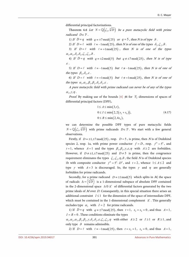
D. C. Mayer
DOI: 10.4236/apm.2019.94017 391 Advances in Pure Mathematics
differential principal factorizations. Theorem 4.6 Let ( )5
5 ,ζ= N D be a pure metacyclic field with prime radicand ∈D .
1) If =D q with ( )7 mod 25≡ ±q or 5=q , then N is of type ϑ . 2) If = D with ( )1mod 25≡ −
, then N is of one of the types 2 2, ,δ ζ ϑ . 3) If = D with ( )1mod 25≡ +
, then N is of one of the types
1 2 1 2 1 2, , , , , ,α α δ δ ζ ζ ϑ . 4) If =D q with ( )2 mod 5≡ ±q but ( )7 mod 25≡ ±/q , then N is of type
ε . 5) If = D with ( )1mod 5≡ −
but ( )1mod 25≡ −/ , then N is of one of the types 2 2, ,β δ ε .
6) If = D with ( )1mod 5≡ + but ( )1mod 25≡ +/ , then N is of one of
the types 1 2 1 2 1 2, , , , , ,α α β β δ δ ε . A pure metacyclic field with prime radicand can never be of any of the types
3 , ,α γ η . Proof. By making use of the bounds [6] §4 for 5 -dimensions of spaces of
differential principal factors (DPF),
( )( )( )
( )2 4
4
1 min 3, ,
0 min 2, 2 ,
0 min 2, 4 ,
≤ ≤
≤ ≤ +
≤ ≤
A t
I s s
R s
(4.17)
we can determine the possible DPF types of pure metacyclic fields
( )55 ,ζ= N D with prime radicands ∈D . We start with a few general
observations. Firstly, if ( )1, 7 mod 25≡ ± ±D , resp. 5=D , is prime, then N is of Dedekind
species 2, resp. 1a, with prime power conductor =f D , resp. 4 65=f , and 1=t , whence 1=A and the types 1 2, , , ,β β γ ε η with 2≥A are forbidden.
However, if ( )1, 7 mod 25≡ ± ±/D and 5≠D is prime, then the congruence requirement eliminates the types 1 2, , ,ζ ζ η ϑ , the field N is of Dedekind species 1b with composite conductor 4 2 45= ⋅f D , and 2=t , whence 1 2≤ ≤A and type γ with 3=A is discouraged. So, the types γ and η are generally forbidden for prime radicands.
Secondly, for a prime radicand ( )1mod 5≡ ±D which splits in M, the space of radicals 5∆ = D is a 1-dimensional subspace of absolute DPF contained in the 2-dimensional space ′∆⊕∆ of differential factors generated by the two prime ideals of M over D. Consequently, in this special situation there arises an additional constraint 1≤I for the dimension of the space of intermediate DPF, which must be contained in the 1-dimensional complement ′∆ . This generally excludes type 3α with 2=I for prime radicands.
1) If =D q with ( )7 mod 25≡ ±q , then 1=t , 2 4 0= =s s , and thus 1=A , 0= =I R . These conditions eliminate the types
1 2 3 1 2 1 2 1 2, , , , , , , , , , ,α α α β β γ δ δ ε ζ ζ η with either 2≥A or 1≥I or 1≥R , and only type ϑ remains admissible.
2) If = D with ( )1mod 25≡ −, then 2 1= =t s , 4 0=s , and thus 1=A ,
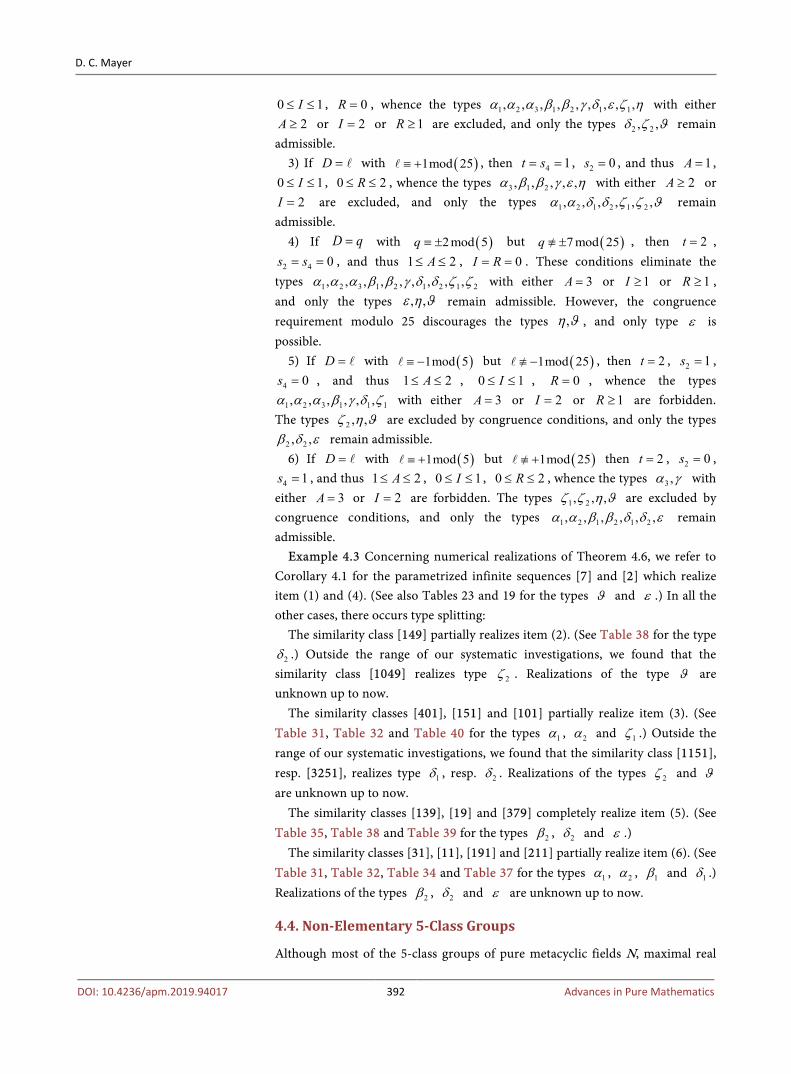
D. C. Mayer
DOI: 10.4236/apm.2019.94017 392 Advances in Pure Mathematics
0 1≤ ≤I , 0=R , whence the types 1 2 3 1 2 1 1, , , , , , , , ,α α α β β γ δ ε ζ η with either 2≥A or 2=I or 1≥R are excluded, and only the types 2 2, ,δ ζ ϑ remain
admissible. 3) If = D with ( )1mod 25≡ +
, then 4 1= =t s , 2 0=s , and thus 1=A , 0 1≤ ≤I , 0 2≤ ≤R , whence the types 3 1 2, , , , ,α β β γ ε η with either 2≥A or
2=I are excluded, and only the types 1 2 1 2 1 2, , , , , ,α α δ δ ζ ζ ϑ remain admissible.
4) If =D q with ( )2 mod 5≡ ±q but ( )7 mod 25≡ ±/q , then 2=t ,
2 4 0= =s s , and thus 1 2≤ ≤A , 0= =I R . These conditions eliminate the types 1 2 3 1 2 1 2 1 2, , , , , , , , ,α α α β β γ δ δ ζ ζ with either 3=A or 1≥I or 1≥R , and only the types , ,ε η ϑ remain admissible. However, the congruence requirement modulo 25 discourages the types ,η ϑ , and only type ε is possible.
5) If = D with ( )1mod 5≡ − but ( )1mod 25≡ −/ , then 2=t , 2 1=s ,
4 0=s , and thus 1 2≤ ≤A , 0 1≤ ≤I , 0=R , whence the types
1 2 3 1 1 1, , , , , ,α α α β γ δ ζ with either 3=A or 2=I or 1≥R are forbidden. The types 2 , ,ζ η ϑ are excluded by congruence conditions, and only the types
2 2, ,β δ ε remain admissible. 6) If = D with ( )1mod 5≡ +
but ( )1mod 25≡ +/ then 2=t , 2 0=s ,
4 1=s , and thus 1 2≤ ≤A , 0 1≤ ≤I , 0 2≤ ≤R , whence the types 3 ,α γ with either 3=A or 2=I are forbidden. The types 1 2, , ,ζ ζ η ϑ are excluded by congruence conditions, and only the types 1 2 1 2 1 2, , , , , ,α α β β δ δ ε remain admissible.
Example 4.3 Concerning numerical realizations of Theorem 4.6, we refer to Corollary 4.1 for the parametrized infinite sequences [7] and [2] which realize item (1) and (4). (See also Tables 23 and 19 for the types ϑ and ε .) In all the other cases, there occurs type splitting:
The similarity class [149] partially realizes item (2). (See Table 38 for the type
2δ .) Outside the range of our systematic investigations, we found that the similarity class [1049] realizes type 2ζ . Realizations of the type ϑ are unknown up to now.
The similarity classes [401], [151] and [101] partially realize item (3). (See Table 31, Table 32 and Table 40 for the types 1α , 2α and 1ζ .) Outside the range of our systematic investigations, we found that the similarity class [1151], resp. [3251], realizes type 1δ , resp. 2δ . Realizations of the types 2ζ and ϑ are unknown up to now.
The similarity classes [139], [19] and [379] completely realize item (5). (See Table 35, Table 38 and Table 39 for the types 2β , 2δ and ε .)
The similarity classes [31], [11], [191] and [211] partially realize item (6). (See Table 31, Table 32, Table 34 and Table 37 for the types 1α , 2α , 1β and 1δ .) Realizations of the types 2β , 2δ and ε are unknown up to now.
4.4. Non-Elementary 5-Class Groups
Although most of the 5-class groups of pure metacyclic fields N, maximal real

D. C. Mayer
DOI: 10.4236/apm.2019.94017 393 Advances in Pure Mathematics
subfields M and pure quintic subfields L are elementary abelian, there occur sparse examples with non-elementary structure. For instance, we have only 8 occurrences within the range 32 10≤ <D of our computations:
1) ( ) 35 25 5Cl ×N C C , ( ) ( ), , ; 1, 2,5 ;6= ∗L M NV V V E for 259 7 37= = ×D
(type γ ), 2) ( ) 7
5 25 5Cl ×N C C , ( ) 35 25 5Cl ×M C C , ( ) ( ), , ; 3,5 ,9 ;2= ∗ ∗L M NV V V E
for 281=D prime (type 1α ), 3) ( ) 5
5 25 5Cl ×N C C , ( ) ( ), , ; 2,3,7 ;4= ∗L M NV V V E for 465 3 5 31= = × ×D (type 2β ),
4) ( ) 55 25 5Cl ×N C C , ( ) ( ), , ; 2,3,7 ;4= ∗L M NV V V E for 473 11 43= = ×D
(type 2β ), 5) ( ) 6
5 25 5Cl ×N C C , ( ) 25 25 5Cl ×M C C , ( )5 25Cl L C
, ( ) ( ), , ; 2 , 4 ,8 ;5= ∗ ∗ ∗L M NV V V E for 502 2 251= = ×D (type 1β ),
6) ( ) 55 25 5Cl ×N C C , ( ) ( ), , ; 2,3,7 ;4= ∗L M NV V V E for 590 2 5 59= = × ×D
(type 2β ), 7) ( ) 2 4
5 25 5Cl ×N C C , ( ) 25 25 5Cl ×M C C , ( ) ( ), , ; 2, 4 ,8 ;5= ∗ ∗L M NV V V E
for 2620 2 5 31= = × ×D (type 1β ), 8) ( ) 4
5 25 5Cl ×N C C , ( )5 25 5Cl ×M C C, ( )5 25Cl L C
, ( ) ( ), , ; 2 ,3 ,6 ;3= ∗ ∗ ∗L M NV V V E for 955 5 191= = ×D (type 2α ).
However, outside the range of systematic computations, we additionally found:
a) ( ) 35 25 5Cl ×N C C , ( )5 25 5Cl ×M C C
, ( )5 25Cl L C,
( ) ( ), , ; 2 ,3 ,7 ;4= ∗ ∗ ∗L M NV V V E for 1049=D prime (type 2ζ ), b) ( ) 2 6
5 25 5Cl ×N C C , ( ) 35 25 5Cl ×M C C , ( ) ( ), , ; 3,5 ,10 ;3= ∗ ∗L M NV V V E
for 3001=D prime (type 2α ), c) ( ) 5 4
5 25 5Cl ×N C C , ( ) 2 35 25 5Cl ×M C C , ( ) 2
5 25 5Cl ×L C C , ( ) ( ), , ; 4 ,7 ,14 ;3= ∗ ∗ ∗L M NV V V E for 3251=D prime (type 2δ ),
d) ( ) 2 25 25 5Cl ×N C C , ( )5 25 5Cl ×M C C
, ( )5 25Cl L C,
( ) ( ), , ; 2 ,3 ,6 ;3= ∗ ∗ ∗L M NV V V E for 5849=D prime (type 2δ ). We point out that in all of the last four examples, the normal field N is a Polya
field, since the radicands D are primes ( )1mod 25≡ ±, the conductors are
primes = f , and thus all primitive ambiguous ideals are principal, generated by the radical 5δ = D and its powers. Consequently, there seems to be no upper bound for the complexity of 5-class groups ( )5Cl N of pure metacyclic Polya fields N in Theorem 4.4.
4.5. Refinement of DPF Types by Similarity Classes
Based on the definition of similarity classes and prototypes in §4.2, on the explicit listing of all prototypes in the range between 2 and 103 in Tables 27-30, and on theoretical foundations in §4.3, we are now in the position to establish the intended refinement of our 13 differential principal factorization types into similarity classes in Tables 31-43, as far as the range of our computations for normalized radicands 32 10≤ <D is concerned. The cardinalities M refine the statistical evaluation in Table 26.

D. C. Mayer
DOI: 10.4236/apm.2019.94017 394 Advances in Pure Mathematics
DPF types are characterized by the multiplet ( ), , ; , ,η ζU A I R , refined Dedekind species, S, by the multiplet ( )0 2 4; , , , ; , ,e t u v m n s s , and 5-class groups by the multiplet ( ), , ;L M NV V V E .
DPF type 1α splits into 3 similarity classes in the ground state ( ) ( ), , 2,3,5=L M NV V V and 2 similarity classes in the first excited state ( ) ( ), , 3,5,9=L M NV V V . Summing up the partial frequencies 6+3 of these states in Table 31 yields the modest absolute frequency 9 of type 1α in the range
32 10≤ <D , as given in Table 26. The logarithmic subfield unit index of type
1α is restricted to the single value 2=E . Type 1α is the unique type with 2-dimensional relative principal factorization, 2=R .
The logarithmic subfield unit index of DPF type 2α can take two values, either 3=E or 1=E . Type 2α with = 3E splits into 5 similarity classes in the ground state ( ) ( ), , 1,1, 2=L M NV V V and 6 similarity classes in the first excited state ( ) ( ), , 2,3,6=L M NV V V . Type 2α with 1=E splits into 7 similarity classes in the ground state ( ) ( ), , 2, 2, 4=L M NV V V and 4 similarity classes in the first excited state ( ) ( ), , 3, 4,8=L M NV V V . Summing up the partial frequencies 40 + 7, resp. 24 + 4, of these states in Table 32 yields the considerable absolute frequency 75 of type 2α in the range 32 10≤ <D , as given in Table 26. Type 2α is the unique type with mixed intermediate and relative principal factorization, 1= =I R .
DPF type 3α splits into 4 similarity classes in the ground state ( ) ( ), , 2, 2,5=L M NV V V and 1 similarity class in the first excited state ( ) ( ), , 3, 4,9=L M NV V V . Summing up the partial frequencies 7 + 1 of these states in Table 33 yields the modest absolute frequency 8 of type 3α in the range
32 10≤ <D , as given in Table 26. The logarithmic subfield unit index of type
3α is restricted to the unique value 2=E . Type 3α is the unique type with 2-dimensional intermediate principal factorization, 2=I .
The logarithmic subfield unit index of DPF type 1β can take two values, either 3=E or 5=E . Type 1β with 3=E consists of 3 similarity classes in the ground state ( ) ( ), , 2,3,6=L M NV V V . Type 1β with 5=E splits into 5 similarity classes in the ground state ( ) ( ), , 1, 2, 4=L M NV V V and 2 similarity classes in the first excited state ( ) ( ), , 2, 4,8=L M NV V V . Summing up the partial frequencies 9, resp. 12 + 2, of these states in Table 34 yields the modest absolute frequency 23 of type 1β in the range 32 10≤ <D , as given in Table 26. Type
1β is the unique type with mixed absolute and relative principal factorization, 2=A and 1=R .
DPF type 2β splits into 16 similarity classes in the ground state ( ) ( ), , 1,1,3L M NV V V = and 9 similarity classes in the first excited state ( ) ( ), , 2,3,7L M NV V V = . Summing up the partial frequencies 146 + 15 of these states in Table 35 yields the high absolute frequency 161 of type 2β in the range 32 10D≤ < , as given in Table 26. The logarithmic subfield unit index of type 2β is restricted to the unique value 4E = . Type 2β is the unique type with mixed absolute and intermediate principal factorization, 2A = and
1I = .

D. C. Mayer
DOI: 10.4236/apm.2019.94017 395 Advances in Pure Mathematics
Table 31. Splitting of type 1α , ( ) ( ), , ; , , 2, , ;1,0,2η ζ = − −U A I R : 5 similarity classes.
No. S e0 t u v m n s2 s4 VL VM VN E M |M|
1 1b 2 1 0 1 1 0 0 1 2 3 5 2 31 2
2 1a 6 1 0 1 4 0 0 1 2 3 5 2 155 2
3 1b 2 1 0 1 1 0 0 1 3 5* 9* 2 281 1
4 1b 2 2 0 2 3 0 0 2 3 5 9 2 341 2 5 2 0 1 1' 0 1 0 0 1' 2 3 5 2 401 2
Table 32. Splitting of type 2α , ( ) ( ), , ; , , 2, , ;1,1,1η ζ = − −U A I R : 22 similarity classes.
No. S e0 t u v m n s2 s4 VL VM VN E M |M|
1 1b 2 1 0 1 1 0 0 1 1 1 2 3 11 14
2 1b 2 2 0 2 3 1 0 1 2 2 4 1 33 8
3 1a 6 1 0 1 4 0 0 1 1 1 2 3 55 6
4 1b 2 2 0 2 3 1 0 1 1 1 2 3 82 15
5 1b 2 2 0 2 3 1 0 1 2 3 6 3 123 2
6 1b 2 1 0 1 1 0 0 1 2 2 4 1 131 6
7 2 0 1 1' 0 1 0 0 1' 1 1 2 3 151 3
8 1a 6 1 0 1 4 0 0 1 2 2 4 1 275 2
9 1b 2 2 1 1 4 1 0 1 2 2 4 1 287 1
10 2 0 3 0 3 3 1 1 1 2 3 6 3 418 1
11 2 0 2 0 2 1 0 0 2 2 3 6 3 451 1
12 1a 6 2 0 2 16 1 0 1 2 3 6 3 550 1
13 1b 2 2 0 2 3 0 0 2 3 4 8 1 671 1
14 2 0 3 0 3 3 1 0 2 2 3 6 3 682 1
15 1b 2 1 0 1 1 0 0 1 3 4 8 1 691 1
16 1a 6 2 0 2 16 1 0 1 2 2 4 1 710 4
17 2 0 1 1' 0 1 0 0 1' 2 2 4 1 751 1
18 1b 2 2 0 2 3 0 1 1 3 4 8 1 779 1
19 1b 2 2 1' 1 4 1 0 1' 2 2 4 1 808 2
20 1b 2 3 1 2 12 2 0 1 3 4 8 1 861 1
21 1a 6 1 0 1 4 0 0 1 2* 3* 6* 3 955 1
22 2 0 2 0 2 1 1 0 1 1 1 2 3 982 2
Table 33. Splitting of type 3α , ( ) ( ), , ; , , 2, , ;1,2,0η ζ = − −U A I R : 5 similarity classes.
No. S e0 t u v m n s2 s4 VL VM VN E M |M|
1 1b 2 2 0 2 3 0 1 1 2 2 5 2 319 3 2 2 0 2 0 2 1 0 2 0 2 2 5 2 551 1
3 1b 2 3 0 3 13 1 1 1 3 4 9 2 627 1
4 2 0 2 0 2 1 0 1 1 2 2 5 2 649 2
5 2 0 3 0 3 3 1 1 1 2 2 5 2 957 1

D. C. Mayer
DOI: 10.4236/apm.2019.94017 396 Advances in Pure Mathematics
Table 34. Splitting of type 1β , ( ) ( ), , ; , , 2, , ;2,0,1η ζ = − −U A I R : 10 similarity classes.
No. S e0 t u v m n s2 s4 VL VM VN E M |M|
1 1b 2 3 0 3 13 2 0 1 2 3 6 3 186 7
2 1b 2 1 0 1 1 0 0 1 1 2 4 5 191 3
3 1b 2 2 0 2 3 1 0 1 1 2 4 5 253 4
4 1b 2 2 1' 1 4 1 0 1' 1 2 4 5 302 2
5 2 0 2 0 2 1 1 0 1 1 2 4 5 482 2
6 1b 2 2 1' 1 4 1 0 1' 2* 4* 8* 5 502 1
7 1b 2 2 0 2 3 1 0 1 2 3 6 3 517 1
8 1a 6 2 0 2 16 1 0 1 2 4* 8* 5 620 1
9 2 0 3 1 2 4 2 0 1 2 3 6 3 693 1
10 1a 6 2 0 2 16 1 0 1 1 2 4 5 825 1
Table 35. Splitting of type 2β , ( ) ( ), , ; , , 2, , ;2,1,0η ζ = − −U A I R : 25 similarity classes.
No. S e0 t u v m n s2 s4 VL VM VN E M |M|
1 1b 2 2 0 2 3 1 0 1 1 1 3 4 22 35
2 1b 2 2 0 2 3 1 1 0 1 1 3 4 38 44
3 1b 2 2 1 1 4 1 0 1 1 1 3 4 77 7
4 1a 6 2 0 2 16 1 0 1 1 1 3 4 110 11
5 2 0 3 0 3 3 2 0 1 1 1 3 4 132 5
6 1b 2 2 1 1 4 1 1 0 1 1 3 4 133 7
7 1b 2 1 0 1 1 0 1 0 1 1 3 4 139 4
8 1b 2 3 1 2 12 2 0 1 2 3 7 4 154 3
9 2 0 3 0 3 3 2 1 0 1 1 3 4 174 3
10 1a 6 2 0 2 16 1 1 0 1 1 3 4 190 9
11 1b 2 2 1' 1 4 1 0 1' 1 1 3 4 202 6
12 1b 2 2 0 2 3 0 1 1 2 3 7 4 209 2
13 1b 2 3 0 3 13 2 0 1 2 3 7 4 286 3
14 1a 6 2 1 1 16 1 0 1 1 1 3 4 385 1
15 1b 2 2 1' 1 4 1 1' 0 1 1 3 4 398 7
16 2 0 3 1 2 4 2 1 0 1 1 3 4 399 2
17 1a 6 2 0 2 16 1 0 1 2 3 7* 4 465 1
18 1b 2 2 1 1 4 1 0 1 2 3 7* 4 473 1
19 2 0 3 1 2 4 2 0 1 1 1 3 4 574 3
20 1a 6 2 0 2 16 1 1 0 2 3 7* 4 590 1
21 1b 2 3 1 2 12 2 1 0 2 3 7 4 609 1
22 1b 2 3 0 3 13 1 1 1 2 3 7 4 638 2
23 1a 6 2 1 1 16 1 1 0 1 1 3 4 665 1
24 2 0 2 0 2 1 1 1 0 1 1 3 4 893 1
25 1b 2 3 0 3 1. 1 0 2 2 3 7 4 902 1
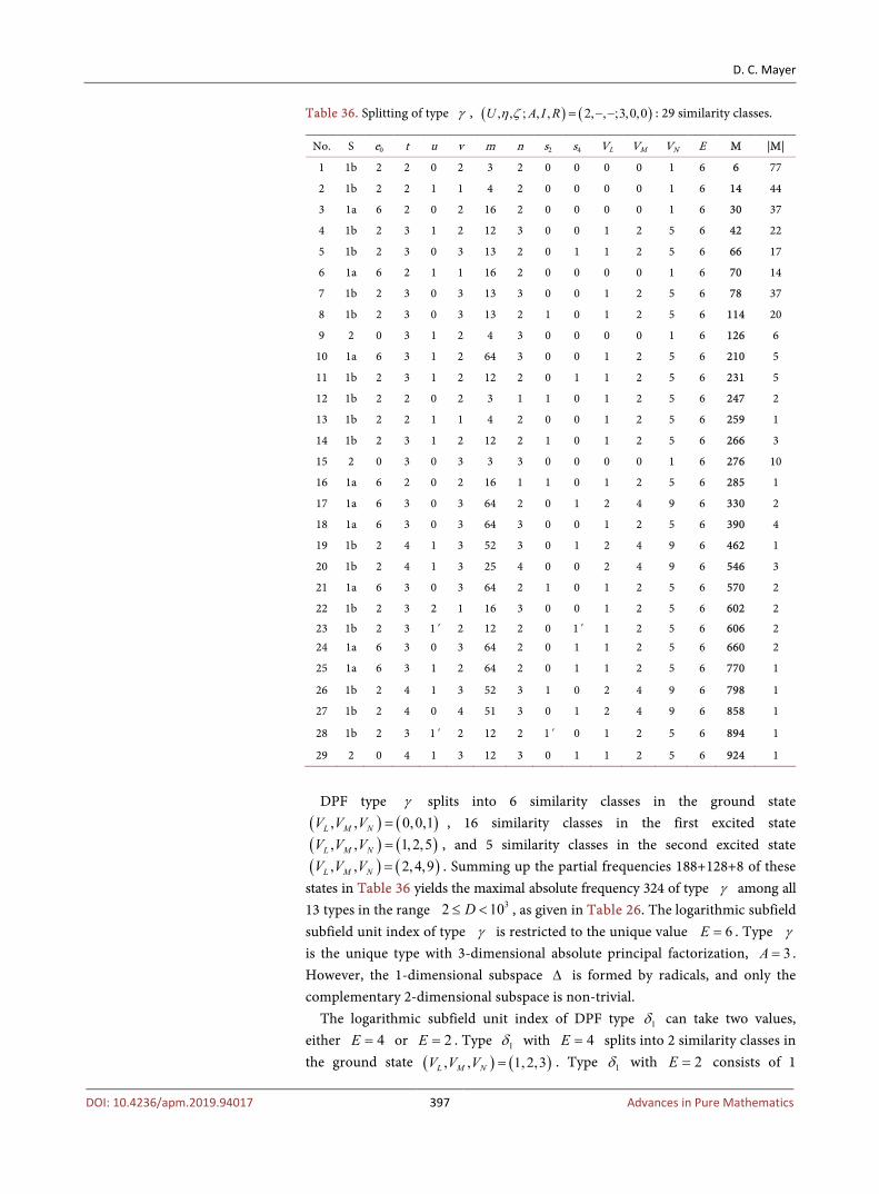
D. C. Mayer
DOI: 10.4236/apm.2019.94017 397 Advances in Pure Mathematics
Table 36. Splitting of type γ , ( ) ( ), , ; , , 2, , ;3,0,0U A I Rη ζ = − − : 29 similarity classes.
No. S e0 t u v m n s2 s4 VL VM VN E M |M|
1 1b 2 2 0 2 3 2 0 0 0 0 1 6 6 77
2 1b 2 2 1 1 4 2 0 0 0 0 1 6 14 44
3 1a 6 2 0 2 16 2 0 0 0 0 1 6 30 37
4 1b 2 3 1 2 12 3 0 0 1 2 5 6 42 22
5 1b 2 3 0 3 13 2 0 1 1 2 5 6 66 17
6 1a 6 2 1 1 16 2 0 0 0 0 1 6 70 14
7 1b 2 3 0 3 13 3 0 0 1 2 5 6 78 37
8 1b 2 3 0 3 13 2 1 0 1 2 5 6 114 20
9 2 0 3 1 2 4 3 0 0 0 0 1 6 126 6
10 1a 6 3 1 2 64 3 0 0 1 2 5 6 210 5
11 1b 2 3 1 2 12 2 0 1 1 2 5 6 231 5
12 1b 2 2 0 2 3 1 1 0 1 2 5 6 247 2
13 1b 2 2 1 1 4 2 0 0 1 2 5 6 259 1
14 1b 2 3 1 2 12 2 1 0 1 2 5 6 266 3
15 2 0 3 0 3 3 3 0 0 0 0 1 6 276 10
16 1a 6 2 0 2 16 1 1 0 1 2 5 6 285 1
17 1a 6 3 0 3 64 2 0 1 2 4 9 6 330 2
18 1a 6 3 0 3 64 3 0 0 1 2 5 6 390 4
19 1b 2 4 1 3 52 3 0 1 2 4 9 6 462 1
20 1b 2 4 1 3 25 4 0 0 2 4 9 6 546 3
21 1a 6 3 0 3 64 2 1 0 1 2 5 6 570 2
22 1b 2 3 2 1 16 3 0 0 1 2 5 6 602 2
23 1b 2 3 1' 2 12 2 0 1' 1 2 5 6 606 2 24 1a 6 3 0 3 64 2 0 1 1 2 5 6 660 2
25 1a 6 3 1 2 64 2 0 1 1 2 5 6 770 1
26 1b 2 4 1 3 52 3 1 0 2 4 9 6 798 1
27 1b 2 4 0 4 51 3 0 1 2 4 9 6 858 1
28 1b 2 3 1' 2 12 2 1' 0 1 2 5 6 894 1
29 2 0 4 1 3 12 3 0 1 1 2 5 6 924 1
DPF type splits into 6 similarity classes in the ground state
, 16 similarity classes in the first excited state , and 5 similarity classes in the second excited state . Summing up the partial frequencies 188+128+8 of these
states in Table 36 yields the maximal absolute frequency 324 of type among all 13 types in the range , as given in Table 26. The logarithmic subfield subfield unit index of type is restricted to the unique value . Type is the unique type with 3-dimensional absolute principal factorization, 3A = . However, the 1-dimensional subspace ∆ is formed by radicals, and only the complementary 2-dimensional subspace is non-trivial.
The logarithmic subfield unit index of DPF type 1δ can take two values, either 4E = or 2E = . Type 1δ with 4E = splits into 2 similarity classes in the ground state ( ) ( ), , 1, 2,3L M NV V V = . Type 1δ with 2E = consists of 1
γ( ) ( ), , 0,0,1L M NV V V =
( ) ( ), , 1, 2,5L M NV V V =
( ) ( ), , 2, 4,9L M NV V V =γ
32 10D≤ <γ 6E = γ

D. C. Mayer
DOI: 10.4236/apm.2019.94017 398 Advances in Pure Mathematics
similarity class in the ground state ( ) ( ), , 3,5,9L M NV V V = . Summing up the partial frequencies 6+1 of these states in Table 37 yields the modest absolute frequency 7 of type 1δ in the range 32 10D≤ < , as given in Table 26. Type
1δ is a type with 1-dimensional relative principal factorization, 1R = . DPF type 2δ splits into 4 similarity classes in the ground state
( ) ( ), , 1,1, 2L M NV V V = and 1 similarity class in the first excited state ( ) ( ), , 2,3,6L M NV V V = . Summing up the partial frequencies 52+1 of these states in Table 38 yields the considerable absolute frequency 53 of type 2δ in the range 32 10D≤ < , as given in Table 26. The logarithmic subfield unit index of type 2δ is restricted to the unique value 3E = . Type 2δ is a type with 1-dimensional intermediate principal factorization, 1I = .
DPF type ε splits into 3 similarity classes in the ground state ( ) ( ), , 0,0,0L M NV V V = , 16 similarity classes in the first excited state ( ) ( ), , 1, 2, 4L M NV V V = , and 3 similarity classes in the second excited state ( ) ( ), , 2, 4,8L M NV V V = . Summing up the partial frequencies 139+61+8 of these states in Table 39 yields the high absolute frequency 208 of type ε in the range
32 10D≤ < , as given in Table 26. The logarithmic subfield unit index of type ε is restricted to the unique value 5E = . Type ε is a type with 2-dimensional absolute principal factorization, 2A = .
The logarithmic subfield unit index of DPF type 1ζ is restricted to the unique value 5E = . Type 1ζ consists of 1 similarity class in the ground state ( ) ( ), , 1, 2, 4L M NV V V = . The frequency 1 of this state in Table 40 coincides with the negligible absolute frequency 1 of type 1ζ in the range 32 10D≤ < , as given in Table 26. Type 1ζ is a type with 1-dimensional relative principal factorization, 1R = .
DPF type 2ζ consists of 3 similarity classes. The modest absolute frequency 5 of type 2ζ in the range 32 10D≤ < , given in Table 26, is the sum 2+1+2 of partial frequencies in Table 41. Type 2ζ only occurs with logarithmic subfield unit index 4E = . It is a type with 1-dimensional intermediate principal factorization, 1I = .
DPF type η splits in 2 similarity classes, [35] and [301]. The modest absolute frequency 7 of type η in the range 32 10D≤ < , given in Table 26, is the sum 6+1 of partial frequencies in Table 42. Type η only occurs with logarithmic subfield unit index 6E = . It is a type with 2-dimensional absolute principal factorization, 2A = . However, it should be pointed out that outside of the range of our systematic investigations we found an excited state
for the similarity class [1505], where has three prime divisors, additionally to the ground state . Table 37. Splitting of type , : 3 similarity classes.
No. S e0 t u v m n s2 s4 VL VM VN E M |M| 1 1b 2 1 0 1 1 0 0 1 3 5 9 2 211 1 2 1b 2 1 0 1 1 0 0 1 1 2 3 4 421 5 3 2 0 2 0 2 1 1 0 1 1 2 3 4 843 1
( ) ( ), , 1, 2,5L M NV V V = 1505 5 7 43= × ×
( ) ( ), , 0,0,1L M NV V V =
1δ ( ) ( ), , ; , , 1, , ;1,0,1U A I Rη ζ = × −

D. C. Mayer
DOI: 10.4236/apm.2019.94017 399 Advances in Pure Mathematics
Table 38. Splitting of type 2δ , ( ) ( ), , ; , , 1, , ;1,1,0U A I Rη ζ = × − : 5 similarity classes.
No. S e0 t u v m n s2 s4 VL VM VN E M |M|
1 1b 2 1 0 1 1 0 1 0 1 1 2 3 19 27
2 2 0 2 0 2 1 1 1 0 1 1 2 3 57 10
3 1a 6 1 0 1 4 0 1 0 1 1 2 3 95 9
4 2 0 1 1' 0 1 0 1' 0 1 1 2 3 149 6
5 1b 2 2 0 2 3 1 1 0 2 3 6 3 377 1
Table 39. Splitting of type ε , ( ) ( ), , ; , , 1, , ;2,0,0U A I Rη ζ = × − : 22 similarity classes.
No. S e0 t u v m n s2 s4 VL VM VN E M |M|
1 1b 2 1 0 1 1 1 0 0 0 0 0 5 2 71
2 1a 6 1 0 1 1 1 0 0 0 0 0 5 10 31
3 2 0 2 0 2 1 2 0 0 0 0 0 5 18 37
4 1a 6 2 1 1 16 2 0 0 1 2 4 5 140 5
5 1b 2 2 0 2 3 2 0 0 1 2 4 5 141 19
6 1b 2 2 0 2 3 1 1 0 1 2 4 5 171 6
7 1a 6 2 0 2 16 2 0 0 1 2 4 5 180 5
8 2 0 3 1 2 4 2 0 0 1 2 4 5 182 1
9 1b 2 2 1 1 4 1 1 0 1 2 4 5 203 2
10 2 0 2 0 2 1 1 1 0 1 2 4 5 218 1
11 1b 2 3 1 2 12 3 0 0 2 4 8 5 273 4
12 1a 6 2 0 2 16 1 1 0 1 2 4 5 290 2
13 1b 2 2 0 2 3 1 1 0 1 2 4 5 298 2
14 1b 2 2 1 1 4 2 0 0 1 2 4 5 329 7
15 1b 2 3 0 3 13 2 1 0 2 4 8 5 348 2
16 1b 2 1 0 1 1 0 1 0 1 2 4 5 379 1
17 1b 2 2 0 2 3 1 0 1 1 2 4 5 422 6
18 2 0 3 1 2 4 2 1 0 1 2 4 5 532 1
19 1a 6 1 0 1 4 0 1 0 1 2 4 5 695 1
20 1b 2 3 0 3 13 3 0 0 2 4 8 5 702 2
21 2 0 2 2 0 4 2 0 0 1 2 4 5 749 1
22 1a 6 1 1 0 4 1 0 0 1 2 4 5 785 1
Table 40. No splitting of type 1ζ , ( ) ( ), , ; , , 1, , ;1,0,1U A I Rη ζ = − × : 1 similarity class.
No. S e0 t u v m n s2 s4 VL VM VN E M |M|
1 2 0 1 1' 0 1 0 0 1' 1 2 4 5 101 1

D. C. Mayer
DOI: 10.4236/apm.2019.94017 400 Advances in Pure Mathematics
Table 41. Splitting of type 2ζ , ( ) ( ), , ; , , 1, , ;1,1,0U A I Rη ζ = − × : 3 similarity classes.
No. S e0 t u v m n s2 s4 VL VM VN E M |M|
1 1a 6 1 1' 0 4 0 0 1' 1 1 3 4 505 2
2 2 0 2 2' 0 4 1 0 1' 1 1 3 4 707 1
3 1a 6 1 1 0 4 0 1 0 1 1 3 4 745 2
Table 42. Splitting of type η , ( ) ( ), , ; , , 1, , ;2,0,0U A I Rη ζ = − × : 2 similarity classes.
No. S e0 t u v m n s2 s4 VL VM VN E M |M|
1 1a 6 1 1 0 4 1 0 0 0 0 1 6 35 6
2 2 0 2 2 0 4 2 0 0 0 0 1 6 301 1
DPF type splits into the unique finite similarity class [5] with only a single element and the infinite parametrized sequence [7] consisting of all prime radicands congruent to . The small absolute frequency 19 of type in the range , given in Table 26, is the sum
in Table 43. Since no theoretical argument disables the occurrence of type for composite radicands D with prime factors 5 and
( )7 mod 25q ≡ ± , we conjecture that such cases will appear in bigger ranges with 310D > . Type ϑ only occurs with logarithmic subfield unit index 5E = , and
is the unique type where every unit of K occurs as norm of a unit of N, that is 0U = .
4.6. Increasing Dominance of DPF Type γ for →T ∞
In this final section, we want to show that the careful book keeping of similarity classes with representative prototypes in Tables 31-43 is useful for the quantitative illumination of many other phenomena. For an explanation, we select the phenomenon of absolute principal factorizations.
The statistical distribution of DPF types in Table 26 has proved that type γ with 324 occurrences, that is 36%, among all 900 fields ( )5
5 ,N Dζ= with normalized radicands in the range 32 10D≤ < is doubtlessly the high champion of all DPF types. This means that there is a clear trend towards the maximal possible extent of 3-dimensional spaces of absolute principal factorizations, 3A = , in spite of the disadvantage that the estimate
( )1 min 3,A T≤ ≤ in the formulas (4.3) and (4.4) of ([6] Cor. 4.1) prohibits type γ for conductors f with 2T ≤ prime divisors.
For the following investigation, we have to recall that the number T of all prime factors of 04 4 4
15etf q q= ⋅
is given by 1T t= + for fields of Dedekind’s species 1, where { }0 2,6e ∈ , and by T t= for fields of Dedekind’s species 2, where 0 0e = .
Conductors f with 4T = prime factors occur in six tables,
ϑ
D q= ( )7 mod 25±
ϑ 32 10D≤ <1 18+ = +5 7
ϑ

D. C. Mayer
DOI: 10.4236/apm.2019.94017 401 Advances in Pure Mathematics
Table 43. Splitting of type , : 2 similarity classes.
No. S e0 t u v m n s2 s4 VL VM VN E M |M|
1 1a 6 0 0 0 1 0 0 0 0 0 0 5 5 1
2 2 0 1 1 0 1 1 0 0 0 0 0 5 7 18
1 case of type 2α in a single similarity class of Table 32, 1 case of type 3α in a single similarity class of Table 33, 7 cases of type 1β in a single similarity class of Table 34, 10 cases of type 2β in 5 similarity classes of Table 35, 126 cases of type γ in 16 similarity classes of Table 36, 8 cases of type ε in 3 similarity classes of Table 39, that is, a total of 153 cases, with respect to the complete range 32 10D≤ < of
our computations. Consequently, we have an increase of type γ from 36.0%,
with respect to the entire database, to 126 82.4%153
= , with respect to 4T = .
The feature is even aggravated for conductors f with 5T = prime factors, which exclusively occur in Table 36. There are 4 similarity classes with 5T = , namely [462], [546], [798], [858], with a total of 6 elements, all (100%) with associated fields of type γ .
5. Conclusions
In this paper, it was our intention to realize Parry’s suggestion ([1] p. 484) concerning a numerical investigation of pure quintic number fields ( )5L D= . For this purpose, we first developed theoretical foundations in a series of preparatory papers [6] [7] [8] [9] which expand the original germs in [12]. Since the non-Galois fields L do not contain the full wealth of arithmetical structures, we had to consider their pure metacyclic normal closures ( )5
5 ,N Dζ= of degree 20.
On the one hand, this enabled us to use the Galois cohomology of the unit group UN with respect to the relative automorphism group ( ) 5GalG N K C=
over the cyclotomic field ( )5K ζ= for defining 13 exhaustive and mutually exclusive differential principal factorization (DPF) types (Table 4 in §3.1), based on the unit norm index ( ) ( )( )0
/# , : 5UN K N K NH G U U N U= = , where
0 2U≤ ≤ , which is connected with the order of the group of primitive ambiguous principal ideals ( ) ( )1 1
/# , : 5UN N K KH G U += = via the
Takagi/Hasse/Iwasawa-Theorem on the Herbrand quotient of UN, and on a natural decomposition 1U A I R+ = + + into the dimensions of the 5 -vector spaces of absolute, intermediate and relative differential principal factors ([6], eqn. (6.3)).
On the other hand, our theory of the relatively cyclic quintic Kummer extension N/K as a 5-ring class field modulo the conductor /N Kf f= over K admitted the calculation of the multiplicity ( )m m f= of the conductor f (§2), which is the number of non-isomorphic pure metacyclic fields N sharing the
ϑ ( ) ( ), , ; , , 0, , ;1,0,0U A I Rη ζ = × ×

D. C. Mayer
DOI: 10.4236/apm.2019.94017 402 Advances in Pure Mathematics
common conductor f and forming a multiplet ( )1, , mN N [8].
Equipped with this theoretical background, we were able to develop our Classification Algorithm 3.1 in §3.2, and to prove that it determines the DPF type of L and N in finitely many steps. It also decides whether the normal field N is a Polya field or not. (It is known that L is a (trivial!) Polya field if and only if it possesses class number 1Lh = [6].)
The algorithm was implemented as a Magma program script [3] [4] [5] and applied to the 900 fields N with normalized fifth power free radicands in the range 32 10D≤ < , after some preliminary experiments with Pari/GP [2]. The result is documented in the twenty Tables 6-25 of §3.4. It is in perfect accordance with our theoretical predictions in 1991 [12]. Actually, each type occurs indeed, the most hardboiled type 2ζ not earlier than for the radicand
505D = , and it is interesting to study the statistical distribution of the types in §4.1, Table 6. Concerning the reliability of our extensive database, and for understanding the degree of precision contained in our paper, we point out that all tables have been thoroughly double checked with respect to misprints and copy-paste errors for at least three times.
Nevertheless, after the completion of the statistics in §4, we came to the conviction that for deeper insight into the arithmetical structure of pure metacyclic fields N, the prime factorization of the class field theoretic conductor f of the abelian extension N/K (invariants 0 2 4; , , ; , ,e t u v n s s ) and the primary invariants of all involved 5-class groups, partially given by the 5-valuations ( ), , ;L M NV V V E , should be taken in consideration. In the last section, we present a corresponding refinement of the DPF types in similarity classes (§4.2), which is very useful for various applications. It reduces the number 900 of investigated radicands to 134 representative prototypes (§4.5). The remaining 766 radicands, which are bigger than the prototype of their similarity class, only reproduce the arithmetical invariants of the prototype and do not provide any additional relevant information. The rare phenomenon of non-elementary 5-class groups is documented in §4.4. Theorems on DPF-types of members of multiplets are proved in §4.3, and the striking dominance of type γ with 3-dimensional (maximal) absolute principal factorization for radicands with three and more prime divisors is presented and discussed in §4.6.
Acknowledgements We gratefully acknowledge that our research was supported by the Austrian Science Fund (FWF): project P 26008-N25. This work is dedicated to the memory of Charles J. Parry († 25 December 2010) who suggested a numerical investigation of pure quintic number fields. We are indebted to the anonymous referees for valuable suggestions concerning an improvement of the paper’s layout.
Conflicts of Interest The author declares no conflicts of interest regarding the publication of this pa-per.
D. C. Mayer
DOI: 10.4236/apm.2019.94017 403 Advances in Pure Mathematics
References [1] Parry, C.J. (1975) Class Number Relations in Pure Quintic Fields. Symposia Ma-
thematica, 15, 475-485.
[2] PARI Developer Group (2018) PARI/GP, Version 64 bit 2.11.1, Bordeaux. http://pari.math.u-bordeaux.fr
[3] Bosma, W., Cannon, J. and Playoust, C. (1997) The Magma Algebra System. I. The User Language. Journal of Symbolic Computation, 24, 235-265. https://doi.org/10.1006/jsco.1996.0125
[4] Bosma, W., Cannon, J.J., Fieker, C. and Steels, A., Eds. (2018) Handbook of Magma functions. Edition 2.24, Sydney.
[5] MAGMA Developer Group (2018) MAGMA Computational Algebra System. Ver-sion 2.24-3, Sydney. http://magma.maths.usyd.edu.au
[6] Mayer, D.C. (2018) Differential Principal Factors and Polya Property of Pure Meta-cyclic Fields. Accepted by Int. J. Number Theory. arXiv:1812.02436v1 [math.NT]
[7] Mayer, D.C. (2018) Similarity Classes and Prototypes of Pure Metacyclic Fields. Preprint.
[8] Mayer, D.C. (2018) Homogeneous Multiplets of Pure Metacyclic Fields. Preprint.
[9] Mayer, D.C. (2018) Coarse Cohomology Types of Pure Metacyclic Fields. ar-Xiv:1812.09854v1 [math.NT]
[10] Barrucand, P. and Cohn, H. (1970) A Rational Genus, Class Number Divisibility, and Unit Theory for Pure Cubic Fields. Journal of Number Theory, 2, 7-21. https://doi.org/10.1016/0022-314X(70)90003-X
[11] Barrucand, P. and Cohn, H. (1971) Remarks on Principal Factors in a Relative Cu-bic Field. Journal of Number Theory, 3, 226-239. https://doi.org/10.1016/0022-314X(71)90040-0
[12] Mayer, D.C. (1991) Classification of Dihedral Fields. Preprint, Department of Computer Science, University of Manitoba, Manitoba.
[13] Mayer, D.C. (1993) Discriminants of Metacyclic Fields. Canadian Mathematical Bulletin, 36, 103-107. https://doi.org/10.4153/CMB-1993-015-x
[14] Kobayashi, H. (2016) Class Numbers of Pure Quintic Fields. Journal of Number Theory, 160, 463-477. https://doi.org/10.1016/j.jnt.2015.09.017
[15] Kobayashi, H. (2016) Class Numbers of Pure Quintic Fields. Ph.D. Thesis, Osaka University Knowledge Archive (OUKA).
[16] Aouissi, S., Mayer, D.C., Ismaili, M.C., Talbi, M. and Azizi, A. (2018) 3-Rank of Ambiguous Class Groups in Cubic Kummer Extensions. arXiv:1804.00767v4 [math.NT]
[17] Aouissi, S., Mayer, D.C. and Ismaili, M.C. (2018) Structure of Relative Genus Fields of Cubic Kummer Extensions. arXiv:1808.04678v1 [math.NT]
[18] Iimura, K. (1977) A Criterion for the Class Number of a Pure Quintic Field to Be Divisible by 5. Journal für die Reine und Angewandte Mathematik, 292, 201-210.
Related Documents