TABLE OF CONTENTS S.NO CHAPTER NO. TOPICS PAGE NO. UNIT-I INTRODUCTION TO DBMS 1 1.1 File Systems Organization - Sequential, Pointer, Indexed, Direct 1 2 1.2 Purpose of Database System 8 3 1.3 Database System Terminologies 12 4 1.4 Database characteristics 14 5 1.5 Data models 16 6 1.6 Types of data models 17 7 1.7 Components of DBMS 19 8 1.8 Relational Algebra 21 9 1.9 LOGICAL DATABASE DESIGN: Relational DBMS 28 10 1.10 Codd's Rule 28 11 1.11 Entity-Relationship model 28 12 1.12 Extended ER Normalization 28 13 1.13 Functional Dependencies, Anomaly- 1NF to 5NF 31 14 1.14 Domain Key Normal Form 35 15 1.15 Denormalization 41 UNIT-II SQL & QUERY OPTIMIZATION 16 2.1 SQL Standards 67 17 2.2 Data types 68 18 2.3 Database Objects 69 19 2.4 DDL 72 20 2.5 DML 74 21 2.6 DCL 80 22 2.7 TCL 81 23 2.8 Embedded SQL 82 24 2.9 Static Vs Dynamic SQL 83 25 2.10 Query Processing and Optimization 84 26 2.11 Heuristics and Cost Estimates in Query Optimization. 84 UNIT- III TRANSACTION PROCESSING AND CONCURRENCY CONTROL 27 3.1 Introduction 103 28 3.2 Properties of Transaction 106 29 3.3 Serializability 123 30 3.4 Concurrency Control 127 31 3.5 Locking Mechanisms 132 32 3.6 Two Phase Commit Protocol 135 33 3.7 Dead lock 140

Welcome message from author
This document is posted to help you gain knowledge. Please leave a comment to let me know what you think about it! Share it to your friends and learn new things together.
Transcript

TABLE OF CONTENTS
S.NO CHAPTER
NO.
TOPICS PAGE NO.
UNIT-I INTRODUCTION TO DBMS
1 1.1 File Systems Organization - Sequential, Pointer,
Indexed, Direct
1
2 1.2 Purpose of Database System 8
3 1.3 Database System Terminologies 12
4 1.4 Database characteristics 14
5 1.5 Data models 16
6 1.6 Types of data models 17
7 1.7 Components of DBMS 19
8 1.8 Relational Algebra 21
9 1.9 LOGICAL DATABASE DESIGN: Relational
DBMS
28
10 1.10 Codd's Rule 28
11 1.11 Entity-Relationship model 28
12 1.12 Extended ER Normalization 28
13 1.13 Functional Dependencies, Anomaly- 1NF to 5NF 31
14 1.14 Domain Key Normal Form 35
15 1.15 Denormalization 41
UNIT-II SQL & QUERY OPTIMIZATION
16 2.1 SQL Standards 67
17 2.2 Data types 68
18 2.3 Database Objects 69
19 2.4 DDL 72
20 2.5 DML 74
21 2.6 DCL 80
22 2.7 TCL 81
23 2.8 Embedded SQL 82
24 2.9 Static Vs Dynamic SQL 83
25 2.10 Query Processing and Optimization 84
26 2.11 Heuristics and Cost Estimates in Query
Optimization.
84
UNIT- III TRANSACTION PROCESSING AND CONCURRENCY CONTROL
27 3.1 Introduction 103
28 3.2 Properties of Transaction 106
29 3.3 Serializability 123
30 3.4 Concurrency Control 127
31 3.5 Locking Mechanisms 132
32 3.6 Two Phase Commit Protocol 135
33 3.7 Dead lock 140
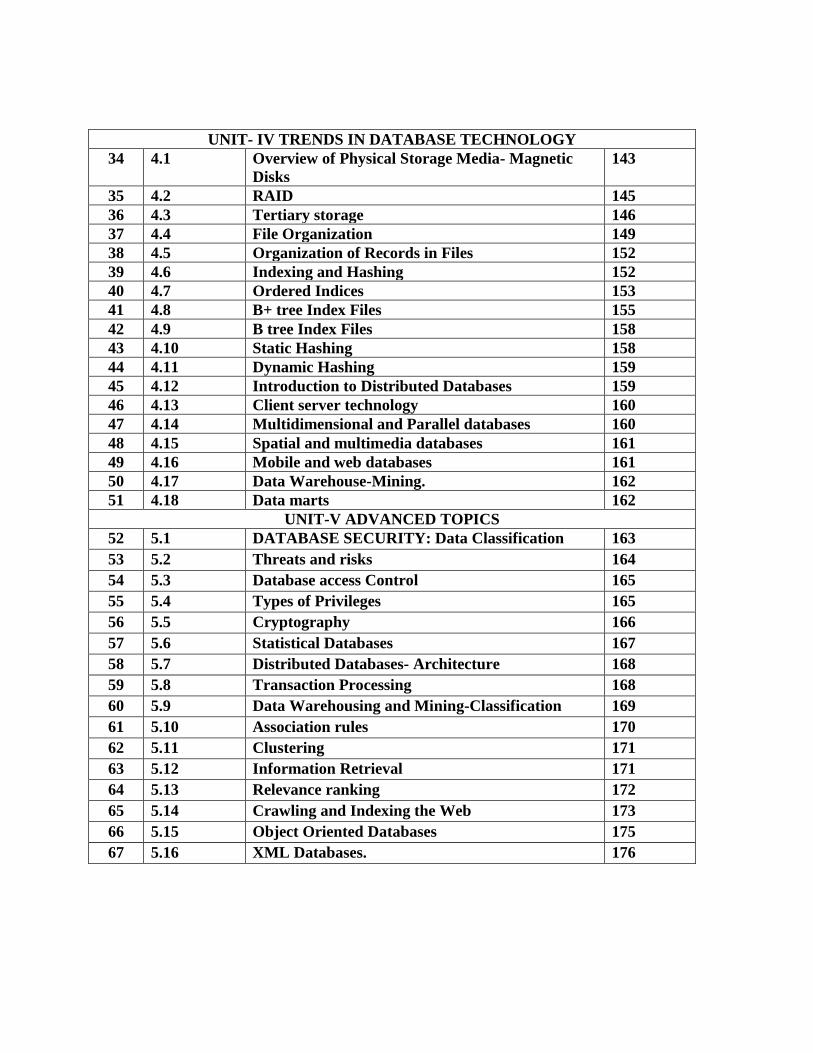
UNIT- IV TRENDS IN DATABASE TECHNOLOGY
34 4.1 Overview of Physical Storage Media- Magnetic
Disks
143
35 4.2 RAID 145
36 4.3 Tertiary storage 146
37 4.4 File Organization 149
38 4.5 Organization of Records in Files 152
39 4.6 Indexing and Hashing 152
40 4.7 Ordered Indices 153
41 4.8 B+ tree Index Files 155
42 4.9 B tree Index Files 158
43 4.10 Static Hashing 158
44 4.11 Dynamic Hashing 159
45 4.12 Introduction to Distributed Databases 159
46 4.13 Client server technology 160
47 4.14 Multidimensional and Parallel databases 160
48 4.15 Spatial and multimedia databases 161
49 4.16 Mobile and web databases 161
50 4.17 Data Warehouse-Mining. 162
51 4.18 Data marts 162
UNIT-V ADVANCED TOPICS
52 5.1 DATABASE SECURITY: Data Classification 163
53 5.2 Threats and risks 164
54 5.3 Database access Control 165
55 5.4 Types of Privileges 165
56 5.5 Cryptography 166
57 5.6 Statistical Databases 167
58 5.7 Distributed Databases- Architecture 168
59 5.8 Transaction Processing 168
60 5.9 Data Warehousing and Mining-Classification 169
61 5.10 Association rules 170
62 5.11 Clustering 171
63 5.12 Information Retrieval 171
64 5.13 Relevance ranking 172
65 5.14 Crawling and Indexing the Web 173
66 5.15 Object Oriented Databases 175
67 5.16 XML Databases. 176

CS6302 DATABASE MANAGEMENT SYSTEMS L T P C 3 0 0 3
UNIT I INTRODUCTION TO DBMS 10 File Systems Organization - Sequential, Pointer, Indexed, Direct - Purpose of Database System- Database System Terminologies-Database characteristics- Data models – Types of data models –Components of DBMS- Relational Algebra. LOGICAL DATABASE DESIGN: Relational DBMS -Codd's Rule - Entity-Relationship model - Extended ER Normalization – Functional Dependencies, Anomaly- 1NF to 5NF- Domain Key Normal Form – Denormalization UNIT II SQL & QUERY OPTIMIZATION 8 SQL Standards - Data types - Database Objects- DDL-DML-DCL-TCL-Embedded SQL-Static Vs Dynamic SQL - QUERY OPTIMIZATION: Query Processing and Optimization - Heuristics and Cost Estimates in Query Optimization. UNIT III TRANSACTION PROCESSING AND CONCURRENCY CONTROL 8 Introduction-Properties of Transaction- Serializability- Concurrency Control – Locking Mechanisms-Two Phase Commit Protocol-Dead lock. UNIT IV TRENDS IN DATABASE TECHNOLOGY 10 Overview of Physical Storage Media – Magnetic Disks – RAID – Tertiary storage – File Organization –Organization of Records in Files – Indexing and Hashing –Ordered Indices – B+ tree Index Files – B tree Index Files – Static Hashing – Dynamic Hashing - Introduction to Distributed Databases- Client server technology- Multidimensional and Parallel databases- Spatial and multimedia databases-Mobile and web databases- Data Warehouse-Mining- Data marts. UNIT V ADVANCED TOPICS 9 DATABASE SECURITY: Data Classification-Threats and risks – Database access Control – Types of Privileges –Cryptography- Statistical Databases.- Distributed Databases-Architecture-Transaction Processing-Data Warehousing and Mining-Classification-Association rules-Clustering-Information Retrieval- Relevance ranking-Crawling and Indexing the Web- Object Oriented Databases-XML Databases.
TOTAL: 45 PERIODS TEXT BOOK: 1. Ramez Elmasri and Shamkant B. Navathe, “Fundamentals of Database Systems”, Fifth Edition, Pearson Education, 2008. REFERENCES: 1. Abraham Silberschatz, Henry F. Korth and S. Sudharshan, “Database System Concepts”, Sixth Edition, Tata Mc Graw Hill, 2011. 2. C.J.Date, A.Kannan and S.Swamynathan, “An Introduction to Database Systems”, Eighth Edition, Pearson Education, 2006. 3. Atul Kahate, “Introduction to Database Management Systems”, Pearson Education, New Delhi,2006. 4. Alexis Leon and Mathews Leon, “Database Management Systems”, Vikas Publishing House Private Limited, New Delhi, 2003. 5. Raghu Ramakrishnan, “Database Management Systems”, Fourth Edition, Tata Mc Graw Hill, 2010. 6. G.K.Gupta, “Database Management Systems”, Tata Mc Graw Hill, 2011. 7. Rob Cornell, “Database Systems Design and Implementation”, Cengage Learning, 2011.

UNIT I INTRODUCTION TO DBMS 10/10
File Systems Organization - Sequential, Pointer, Indexed, Direct - Purpose of Database System-
Database System Terminologies-Database characteristics- Data models – Types of data
models – Components of DBMS- Relational Algebra. LOGICAL DATABASE DESIGN:
Relational DBMS - Codd's Rule - Entity-Relationship model - Extended ER Normalization –
Functional Dependencies, Anomaly- 1NF to 5NF- Domain Key Normal Form – Denormalization
What is database?
Database:
A very large collection of related data
Models a real world enterprise:
Entities (e.g., teams, games / students, courses)
Relationships (e.g., The Celtics are playing in the Final!)
Even active components (e.g. “business logic”)
DBMS: A software package/system that can be used to store, manage and retrieve data
form databases
Database System: DBMS+data (+ applications)
Why Study Database:
Shift from computation to information
Always true for corporate computing
More and more true in the scientific world and of course, Web
DBMS encompasses much of CS in a practical discipline
OS, languages, theory, AI, logic
Why Databases
Why not store everything on flat files: use the file system of the OS, cheap/simple…
Name, Course, Grade
John Smith, CS112, B
Mike Stonebraker, CS234, A
1

Jim Gray, CS560, A
John Smith, CS560, B+
Yes, but not scalable…
Problem 1
Data redundancy and inconsistency
Multiple file formats, duplication of information in different files
Name, Course, Email, Grade
John Smith, [email protected], CS112, B
Mike Stonebraker, [email protected], CS234, A
Jim Gray, CS560, [email protected], A
John Smith, CS560, [email protected], B+
Why this a problem?
Wasted space
Potential inconsistencies (multiple formats, John Smith vs Smith J.)
Problem 2
Data retrieval:
Find the students who took CS560
Find the students with GPA > 3.5
For every query we need to write a program!
We need the retrieval to be:
Easy to write
Execute efficiently
Problem 3
Data Integrity
No support for sharing:
Prevent simultaneous modifications
2

No coping mechanisms for system crashes
No means of Preventing Data Entry Errors
Security problems
Database systems offer solutions to all the above problems.
A database is a collection of data elements (facts) stored in a computer in a systematic way,
such that a computer program can consult it to answer questions. The answers to those questions
become information that can be used to make decisions that may not be made with the data
elements alone. The computer program used to manage and query a database is known as a
database management system (DBMS). So a database is a collection of related data that we can
use for
Defining - specifying types of data
Constructing - storing & populating
Manipulating - querying, updating, reporting
A Database Management System (DBMS) is a software package to facilitate the creation and
maintenance of a computerized database. A Database System (DBS) is a DBMS together with
the data itself.
Features of a database:
It is a persistent (stored) collection of related data.
The data is input (stored) only once.
The data is organized (in some fashion).
The data is accessible and can be queried (effectively and efficiently).
DBMS:
• Collection of interrelated data
• Set of programs to access the data
• DMBS contains information about a particular enterprise
• DBMS provides an environment that it both convenient and efficient to use
Purpose of DBMS:
3

Database management systems were developed to handle the following difficulties of typical
file-processing systems supported by conventional operating systems:
• Data redundancy and inconsistency
• Difficulty in accessing data
• Data isolation – multiple files and formats
• Integrity problems
• Atomicity of updates
• Concurrent access by multiple users
• Security problems
Introduction to Databases
We live in an information age. By this we mean that, first, we accept the universal fact that
information is required in practically all aspects of human enterprise. The term „enterprise‟ is
used broadly here to mean any organisation of activities to achieve a stated purpose, including
socio-economic activities. Second, we recognise further the importance of efficiently providing
timely relevant information to an enterprise and of the importance of the proper use of
technology to achieve that. Finally, we recognise that the unparallelled development in the
technology to handle information has and will continue to change the way we work and live, ie.
not only does the technology support existing enterprises but it changes them and makes possible
new enterprises that would not have otherwise been viable.
The impact is perhaps most visible in business enterprises where there are strong elements
of competition. This is especially so as businesses become more globalised. The ability to
coordinate activities, for example, across national borders and time zones clearly depends on the
timeliness and quality of information made available. More important perhaps, strategic
decisions made by top management in response to perceived opportunities or threats will decide
the future viability of an enterprise, one way or the other. In other words, in order to manage a
business (or any) enterprise, future development must be properly estimated. Information is a
vital ingredient in this regard.
Information must therefore be collected and analysed in order to make decisions. It is here
that the proper use of technology will prove to be crucial to an enterprise. Up-to-date
management techniques should include computers, since they are very powerful tools for
processing large quantities of information. Collecting and analysing information using computers
4

is facilitated by current Database Technology, a relatively mature technology which is the
subject of this book.
Purpose of Database Systems
1. To see why database management systems are necessary, let's look at a typical
``file-processing system'' supported by a conventional operating system.
The application is a savings bank:
o Savings account and customer records are kept in permanent system files.
o Application programs are written to manipulate files to perform the following
tasks:
Debit or credit an account.
Add a new account.
Find an account balance.
Generate monthly statements.
2. Development of the system proceeds as follows:
o New application programs must be written as the need arises.
o New permanent files are created as required.
o but over a long period of time files may be in different formats, and
o Application programs may be in different languages.
3. So we can see there are problems with the straight file-processing approach:
o Data redundancy and inconsistency
Same information may be duplicated in several places.
All copies may not be updated properly.
o Difficulty in accessing data
May have to write a new application program to satisfy an unusual
request.
E.g. find all customers with the same postal code.
Could generate this data manually, but a long job...
o Data isolation
Data in different files.
Data in different formats.
Difficult to write new application programs.
o Multiple users
Want concurrency for faster response time.
5

Need protection for concurrent updates.
E.g. two customers withdrawing funds from the same account at the
same time - account has $500 in it, and they withdraw $100 and $50.
The result could be $350, $400 or $450 if no protection.
o Security problems
Every user of the system should be able to access only the data they
are permitted to see.
E.g. payroll people only handle employee records, and cannot see
customer accounts; tellers only access account data and cannot see
payroll data.
Difficult to enforce this with application programs.
o Integrity problems
Data may be required to satisfy constraints.
E.g. no account balance below $25.00.
Again, difficult to enforce or to change constraints with the file-
processing approach.
These problems and others led to the development of database management systems.
File systems vs Database systems:
DBMS are expensive to create in terms of software, hardware, and time invested.
So why use them? Why couldn‟t we just keep all our data in files, and use word
processors to edit the files appropriately to insert, delete, or update data? And we could
write our own programs to query the data! This solution is called maintaining data in flat
files. So what is bad about flat files?
o Uncontrolled redundancy
o Inconsistent data
o Inflexibility
o Limited data sharing
o Poor enforcement of standards
o Low programmer productivity
o Excessive program maintenance
o Excessive data maintenance
6

File System
Data is stored in Different Files in forms of Records
The programs are written time to time as per the requirement to manipulate the data
within files.
A program to debit and credit an account
A program to find the balance of an account
A program to generate monthly statements
Disadvantages of File system over DBMS
Most explicit and major disadvantages of file system when compared to database
managementsystem are as follows:
Data Redundancy- The files are created in the file system as and when required by
anenterprise over its growth path. So in that case the repetition of information about anentity
cannot be avoided.
Eg. The addresses of customers will be present in the file maintaining information
about customers holding savings account and also the address of the customers will be present in
file maintaining the current account. Even when same customer have a saving account and
current account his address will be present at two places.
Data Inconsistency: Data redundancy leads to greater problem than just wasting thestorage
i.e. it may lead to inconsistent data. Same data which has been repeated at severalplaces may not
match after it has been updated at some places.
For example: Suppose the customer requests to change the address for his account in
the Bank and the Program is executed to update the saving bank account file only but hiscurrent
bank account file is not updated. Afterwards the addresses of the same customerpresent in saving
bank account file and current bank account file will not match.Moreover there will be no way to
find out which address is latest out of these two.
Difficulty in Accessing Data: For generating ad hoc reports the programs will not alreadybe
present and only options present will to write a new program to generate requestedreport or to
work manually. This is going to take impractical time and will be more expensive.
For example: Suppose all of sudden the administrator gets a request to generate a list
of all the customers holding the saving banks account who lives in particular locality of the city.
Administrator will not have any program already written to generate that list but say he has a
program which can generate a list of all the customers holding the savings account. Then he can
either provide the information by going thru the list manually to select the customers living in the
particular locality or he can write a new program to generate the new list. Both of these ways
will take large time which would generally be impractical.
Data Isolation: Since the data files are created at different times and supposedly bydifferent
people the structures of different files generally will not match. The data will be scattered in
different files for a particular entity. So it will be difficult to obtain appropriate data.
For example: Suppose the Address in Saving Account file have fields: Add line1, Add
line2, City, State, Pin while the fields in address of Current account are: House No., Street No.,
Locality, City, State, Pin. Administrator is asked to provide the list of customers living in a
particular locality. Providing consolidated list of all the customers will require looking in both
7
files. But they both have different way of storing the address. Writing a program to generate such
a list will be difficult.
Integrity Problems: All the consistency constraints have to be applied to database through
appropriate checks in the coded programs. This is very difficult when number such constraint is
very large.
For example: An account should not have balance less than Rs. 500. To enforce this
constraint appropriate check should be added in the program which add a record and the program
which withdraw from an account. Suppose later on this amount limit is
increased then all those check should be updated to avoid inconsistency. These time to time
changes in the programs will be great headache for the administrator.
Security and access control: Database should be protected from unauthorized users. Every
user should not be allowed to access every data. Since application programs are added to the
system
For example: The Payroll Personnel in a bank should not be allowed to access
accounts information of the customers.
Concurrency Problems: When more than one users are allowed to process the database. If
in that environment two or more users try to update a shared data element at about the same time
then it may result into inconsistent data. For example: Suppose Balance of an account is Rs. 500.
And User A and B try to withdraw Rs 100 and Rs 50 respectively at almost the same time using
the Update process.
Update:
1. Read the balance amount.
2. Subtract the withdrawn amount from balance.
3. Write updated Balance value.
Suppose A performs Step 1 and 2 on the balance amount i.e it reads 500 and subtract100 from it.
But at the same time B withdraws Rs 50 and he performs the Update process and he also reads
the balance as 500 subtract 50 and writes back 450. User A will also write his updated Balance
amount as 400. They may update the Balance value in any order depending on various reasons
concerning to system being used by both of the users. So finally the balance will be either equal
to 400 or 450. Both of these values are wrong for the updated balance and so now the balance
amount is having inconsistent value forever.
Sequential Access
The simplest access method is Sequential Access. Information in the file is processed in order,
one record after the other. This mode of access is by far the most common; for example, editors
and compilers usually access files in this fashion.
The bulk of the operations on a file is reads and writes. A read operation reads the next portion of
the file and automatically advances a file pointer, which tracks the I/O location. Similiarly, a
write appends to the end of the file and advances to the end of the newly written material (the
new end of file).
8

File Pointers
When a file is opened, Windows associates a file pointer with the default stream. This file
pointer is a 64-bit offset value that specifies the next byte to be read or the location to receive the
next byte written. Each time a file is opened, the system places the file pointer at the beginning
of the file, which is offset zero. Each read and write operation advances the file pointer by the
number of bytes being read and written. For example, if the file pointer is at the beginning of the
file and a read operation of 5 bytes is requested, the file pointer will be located at offset 5
immediately after the read operation. As each byte is read or written, the system advances the file
pointer. The file pointer can also be repositioned by calling the SetFilePointer function.
When the file pointer reaches the end of a file and the application attempts to read from the file,
no error occurs, but no bytes are read. Therefore, reading zero bytes without an error means the
application has reached the end of the file. Writing zero bytes does nothing.
An application can truncate or extend a file by using the SetEndOfFile function. This function
sets the end of file to the current position of the file pointer.
Indexed allocation
– Each file has its own index block(s) of pointers to its data blocks
• Logical view
Need index table
Random access
9

• Dynamic access without external fragmentation, but have overhead of index block
• Mapping from logical to physical in a file of maximum size of 256K bytes and block size of 512 bytes. We need only 1 block for index table
Q
• LA Q512
R
• Q = displacement into index table
• R = displacement into block
Mapping from logical to physical in a file of unbounded length (block size of 512 words)
Linked scheme – Link blocks of index table (no limit on size
Q1
• LA Q512 ×511
R1
Q1 = block of index table R1 is used as follows:
Q2
• R1 /512
R2
Q2 = displacement into block of index table
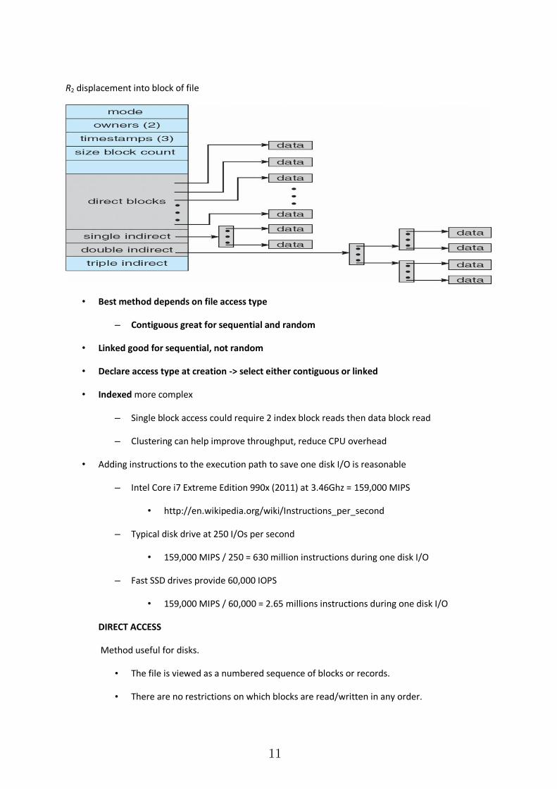
R2 displacement into block of file:
Two-level index (4K blocks could store 1,024 four-byte pointers in outer index -> 1,048,567 data blocks
and file size of up to 4GB)
Q1
LA 512 / 512
R1
Q1 = displacement into outer-index
R1 is used as follows:
Q2
R1 /512
R2
Q2 = displacement into block of index table
10
R2 displacement into block of file
• Best method depends on file access type
– Contiguous great for sequential and random
• Linked good for sequential, not random
• Declare access type at creation -> select either contiguous or linked
• Indexed more complex
– Single block access could require 2 index block reads then data block read
– Clustering can help improve throughput, reduce CPU overhead
• Adding instructions to the execution path to save one disk I/O is reasonable
– Intel Core i7 Extreme Edition 990x (2011) at 3.46Ghz = 159,000 MIPS
• http://en.wikipedia.org/wiki/Instructions_per_second
– Typical disk drive at 250 I/Os per second
• 159,000 MIPS / 250 = 630 million instructions during one disk I/O
– Fast SSD drives provide 60,000 IOPS
• 159,000 MIPS / 60,000 = 2.65 millions instructions during one disk I/O
DIRECT ACCESS
Method useful for disks.
• The file is viewed as a numbered sequence of blocks or records.
• There are no restrictions on which blocks are read/written in any order.
11

• User now says "read n" rather than "read next".
• "n" is a number relative to the beginning of file, not relative to an absolute physical disk
location.
purpose of database system
Database management systems were developed to handle the following difficulties of typical
file-processing systems supported by conventional operating systems:
• Data redundancy and inconsistency
• Difficulty in accessing data
• Data isolation – multiple files and formats
• Integrity problems
• Atomicity of updates
• Concurrent access by multiple users
• Security problems
Purpose of Database Systems
4. To see why database management systems are necessary, let's look at a typical
``file-processing system'' supported by a conventional operating system.
The application is a savings bank:
o Savings account and customer records are kept in permanent system files.
o Application programs are written to manipulate files to perform the following
tasks:
Debit or credit an account.
Add a new account.
Find an account balance.
Generate monthly statements.
5. Development of the system proceeds as follows:
o New application programs must be written as the need arises.
o New permanent files are created as required.
o but over a long period of time files may be in different formats, and
o Application programs may be in different languages.
6. So we can see there are problems with the straight file-processing approach:
o Data redundancy and inconsistency
12

Same information may be duplicated in several places.
All copies may not be updated properly.
o Difficulty in accessing data
May have to write a new application program to satisfy an unusual
request.
E.g. find all customers with the same postal code.
Could generate this data manually, but a long job...
o Data isolation
Data in different files.
Data in different formats.
Difficult to write new application programs.
o Multiple users
Want concurrency for faster response time.
Need protection for concurrent updates.
E.g. two customers withdrawing funds from the same account at the
same time - account has $500 in it, and they withdraw $100 and $50.
The result could be $350, $400 or $450 if no protection.
o Security problems
Every user of the system should be able to access only the data they
are permitted to see.
E.g. payroll people only handle employee records, and cannot see
customer accounts; tellers only access account data and cannot see
payroll data.
Difficult to enforce this with application programs.
o Integrity problems
Data may be required to satisfy constraints.
E.g. no account balance below $25.00.
Again, difficult to enforce or to change constraints with the file-
processing approach.
These problems and others led to the development of database management systems.
13
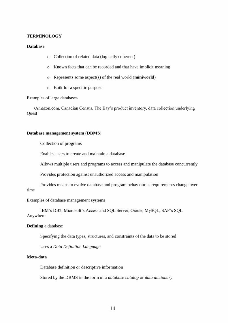
TERMINOLOGY
Database
o Collection of related data (logically coherent)
o Known facts that can be recorded and that have implicit meaning
o Represents some aspect(s) of the real world (miniworld)
o Built for a specific purpose
Examples of large databases
•Amazon.com, Canadian Census, The Bay‟s product inventory, data collection underlying
Quest
Database management system (DBMS)
Collection of programs
Enables users to create and maintain a database
Allows multiple users and programs to access and manipulate the database concurrently
Provides protection against unauthorized access and manipulation
Provides means to evolve database and program behaviour as requirements change over
time
Examples of database management systems
IBM‟s DB2, Microsoft‟s Access and SQL Server, Oracle, MySQL, SAP‟s SQL
Anywhere
Defining a database
Specifying the data types, structures, and constraints of the data to be stored
Uses a Data Definition Language
Meta-data
Database definition or descriptive information
Stored by the DBMS in the form of a database catalog or data dictionary
14
Phases for designing a database:
Requirements specification and analysis
Conceptual design
e.g., using the Entity-Relationship model
Logical design
e.g., using the relational model
Physical design
Populating a database
Inserting data to reflect the miniworld
Query
Interaction causing some data to be retrieved
uses a Query Language
Manipulating a database
Querying and updating the database to understand/reflect miniworld
Generating reports
Uses a Data Manipulation Language
Application program
Accesses database by sending queries and updates to DBMS
Transaction
An atomic unit of queries and updates that must be executed as a whole
e.g., buying a product, transferring funds, switching co-op streams
15
Data Models:
A characteristic of the database approach is that it provides a level of data abstraction, by
hiding details of data storage that are not needed by most users.
A data model is a collection of concepts that can be used to describe the structure of a
database. The model provides the necessary means to achieve the abstraction.
The structure of a database is characterized by data types, relationships, and constraints
that hold for the data. Models also include a set of operations for specifying retrievals and
updates.
Data models are changing to include concepts to specify the behaviour of the database
application. This allows designers to specify a set of user defined operations that are allowed.
Categories of Data Models
Data models can be categorized in multiple ways.
High level/conceptual data models – provide concepts close to the way users perceive the
data.
Physical data models – provide concepts that describe the details of how data is stored in the
computer. These concepts are generally meant for the specialist, and not the end user.
Representational data models – provide concepts that may be understood by the end user
but not far removed from the way data is organized.
Conceptual data models use concepts such as entities, attributes and relationships.
Entity – represents a real world object or concept
Attribute - represents property of interest that describes an entity, such as name or
salary.
Relationships – among two or more entities, represents an association among two or
more entities.
Representational data models are used most frequently in commercial DBMSs. They include
relational data models, and legacy models such as network and hierarchical models.
Physical data models describe how data is stored in files by representing record formats, record
orderings and access paths.
16

Object data models – a group of higher level implementation data models closer to conceptual
data models
Three Schema Architecture
The goal of the three schema architecture is to separate the user applications and the physical
database. The schemas can be defined at the following levels:
1. The internal level – has an internal schema which describes the physical storage
structure of the database. Uses a physical data model and describes the complete details
of data storage and access paths for the database.
2. The conceptual level – has a conceptual schema which describes the structure of the
database for users. It hides the details of the physical storage structures, and concentrates
on describing entities, data types, relationships, user operations and constraints. Usually a
representational data model is used to describe the conceptual schema.
3. The External or View level – includes external schemas or user vies. Each external
schema describes the part of the database that a particular user group is interested in and
hides the rest of the database from that user group. Represented using the
representational data model.
The three schema architecture is used to visualize the schema levels in a database. The three
schemas are only descriptions of data, the data only actually exists is at the physical level.
Internal Level:
• Deals with physical storage of data
External
View
External
View
Conceptual Schema
Internal Schema
STORED DATABASE
EXTERNAL
VIEW
CONCEPTUAL
LEVEL
INTERNAL
LEVEL
mappings
mappings
17

• Structure of records on disk - files, pages, blocks
• Indexes and ordering of records
• Used by database system programmers Internal Schema
RECORD EMP
LENGTH=44
HEADER: BYTE(5)
OFFSET=0
NAME: BYTE(25)
OFFSET=5
SALARY: FULLWORD
OFFSET=30
DEPT: BYTE(10)
OFFSET=34
.Conceptual Schema:
• Deals with the organisation of the data as a whole
• Abstractions are used to remove unnecessary details of the internal level
• Used by DBAs and application programmers
• Conceptual Schema
CREATE TABLE Employee ( Name VARCHAR(25), Salary
DOUBLE, Dept_Name VARCHAR(10));
External Level:
• Provides a view of the database tailored to a user
• Parts of the data may be hidden
• Data is presented in a useful form
• Used by end users and application programmers
External Schemas Payroll:
String Name
double Salary
Personnel:
char *Name
char *Department
18

Mappings
• Mappings translate information from one level to the next
• External/Conceptual
• Conceptual/Internal
• These mappings provide data independence
• Physical data independence
• Changes to internal level shouldn‟t affect conceptual level
• Logical data independence
• Conceptual level changes shouldn‟t affect external levels
Data Model Architecture:
Components of DBMS
A database management system (DBMS) consists of several components. Each component plays
very important role in the database management system environment. The major components of
database management system are:
Software Hardware Data Procedures Database Access Language
Software
19

The main component of a DBMS is the software. It is the set of programs used to handle the database
and to control and manage the overall computerized database
1. DBMS software itself, is the most important software component in the overall system 2. Operating system including network software being used in network, to share the data of
database among multiple users. 3. Application programs developed in programming languages such as C++, Visual Basic that are
used to to access database in database management system. Each program contains statements that request the DBMS to perform operation on database. The operations may include retrieving, updating, deleting data etc . The application program may be conventional or online workstations or terminals.
Hardware
Hardware consists of a set of physical electronic devices such as computers (together with associated
I/O devices like disk drives), storage devices, I/O channels, electromechanical devices that make
interface between computers and the real world systems etc, and so on. It is impossible to implement
the DBMS without the hardware devices, In a network, a powerful computer with high data processing
speed and a storage device with large storage capacity is required as database server.
Data
Data is the most important component of the DBMS. The main purpose of DBMS is to process the data.
In DBMS, databases are defined, constructed and then data is stored, updated and retrieved to and from
the databases. The database contains both the actual (or operational) data and the metadata (data
about data or description about data).
Procedures
Procedures refer to the instructions and rules that help to design the database and to use the DBMS.
The users that operate and manage the DBMS require documented procedures on hot use or run the
database management system. These may include.
1. Procedure to install the new DBMS. 2. To log on to the DBMS. 3. To use the DBMS or application program. 4. To make backup copies of database. 5. To change the structure of database. 6. To generate the reports of data retrieved from database.
Database Access Language
The database access language is used to access the data to and from the database. The users use the
database access language to enter new data, change the existing data in database and to retrieve
required data from databases. The user write a set of appropriate commands in a database access
language and submits these to the DBMS. The DBMS translates the user commands and sends it to a
specific part of the DBMS called the Database Jet Engine. The database engine generates a set of results
according to the commands submitted by user, converts these into a user readable form called an
Inquiry Report and then displays them on the screen. The administrators may also use the database
access language to create and maintain the databases.
20
The most popular database access language is SQL (Structured Query Language). Relational databases
are required to have a database query language.
Users
The users are the people who manage the databases and perform different operations on the databases
in the database system.There are three kinds of people who play different roles in database system
1. Application Programmers 2. Database Administrators 3. End-Users
Application Programmers
The people who write application programs in programming languages (such as Visual Basic, Java, or
C++) to interact with databases are called Application Programmer.
Database Administrators
A person who is responsible for managing the overall database management system is called database
administrator or simply DBA.
End-Users
The end-users are the people who interact with database management system to perform different
operations on database such as retrieving, updating, inserting, deleting data etc.
Relational Query Languages
• Languages for describing queries on a relational database
• Structured Query Language (SQL)
– Predominant application-level query language
– Declarative
• Relational Algebra
– Intermediate language used within DBMS
– Procedural
What is Algebra?
• A language based on operators and a domain of values
• Operators map values taken from the domain into other domain values
• Hence, an expression involving operators and arguments produces a value in the domain
• When the domain is a set of all relations (and the operators are as described later), we get the
relational algebra
• We refer to the expression as a query and the value produced as the query result
21

Relational Algebra
• Domain: set of relations
• Basic operators: select, project, union, set difference, Cartesian product
• Derived operators: set intersection, division, join
• Procedural: Relational expression specifies query by describing an algorithm (the sequence in
which operators are applied) for determining the result of an expression
Select Operator
• Produce table containing subset of rows of argument table satisfying condition
condition relation
• Example:
Person Hobby=‘stamps’(Person)
Selection Condition
• Operators: <, , , >, =,
• Simple selection condition:
– <attribute> operator <constant>
– <attribute> operator <attribute>
• <condition> AND <condition>
• <condition> OR <condition>
• NOT <condition>
Project Operator
22

Produces table containing subset of columns of argument table
attribute list(relation)
• Example:
Person Name,Hobby(Person)
Set Operators
• Relation is a set of tuples => set operations should apply
• Result of combining two relations with a set operator is a relation => all its elements must be
tuples having same structure
• Hence, scope of set operations limited to union compatible relations
Union Compatible Relations
• Two relations are union compatible if
– Both have same number of columns
– Names of attributes are the same in both
– Attributes with the same name in both relations have the same domain
• Union compatible relations can be combined using union, intersection, and set difference
Cartesian product
• If R and S are two relations, R S is the set of all concatenated tuples <x,y>, where x is a tuple in
R and y is a tuple in S
– (R and S need not be union compatible)
• R S is expensive to compute:
– Factor of two in the size of each row
– Quadratic in the number of rows
23
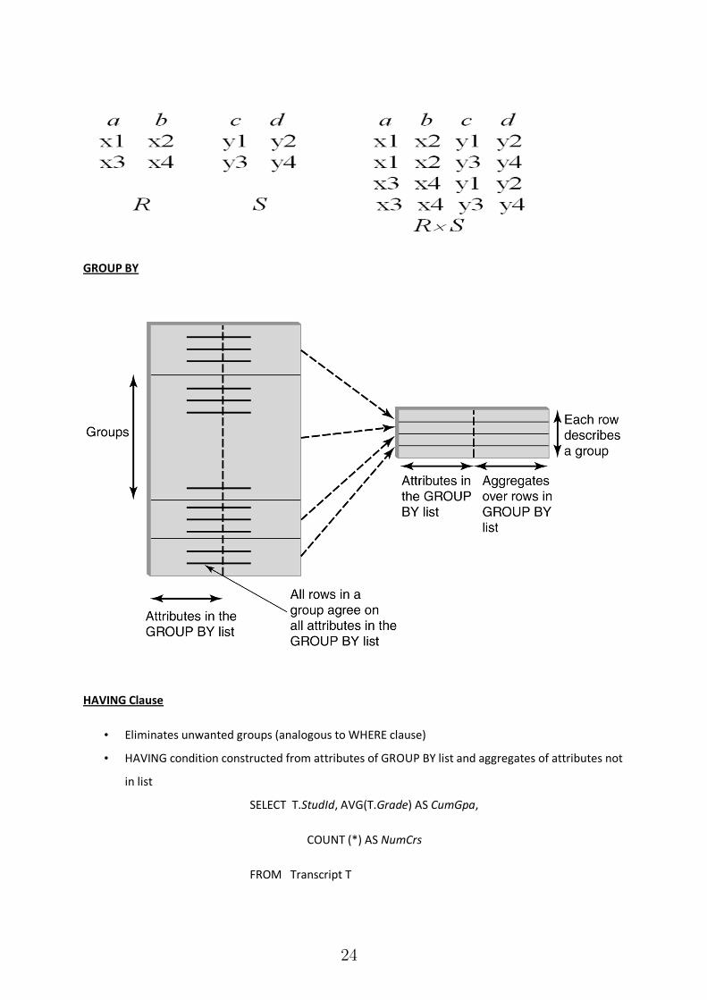
GROUP BY
HAVING Clause
• Eliminates unwanted groups (analogous to WHERE clause)
• HAVING condition constructed from attributes of GROUP BY list and aggregates of attributes not
in list
SELECT T.StudId, AVG(T.Grade) AS CumGpa,
COUNT (*) AS NumCrs
FROM Transcript T
24
WHERE T.CrsCode LIKE ‘CS%’
GROUP BY T.StudId
HAVING AVG (T.Grade) > 3.5.
A Database Management System is a software environment that structures and manipulatesdata,
and ensures data security, recovery, and integrity. The Data Platform relies on a database
management system (RDBMS) to store and maintain all of its data as well as execute all the
associated queries. There are two types of RDBMS : the first group consists of single software
packages which support only a single database, with a single user access and are not scalable (i.e.
cannot handle large amounts of data). Typical examples of this first group are MS Access and
FileMaker. The second group is formed by DBMS composed of one or more programs and their
associated services which support one or many databases for one or many users in ascalable
fashion. For example an enterprise database server can support the HR database,the accounting
database and the stocks database all at the same time. Typical examples ofthis second group
include MySQL, MS SQL Server, Oracle and DB2. The DBMS selected for the Data Platform is
MS SQL Server from the second group.
Table
A table is set of data elements that has a horizontal dimension (rows) and a vertical dimension
(columns) in a relational database system. A table has a specified number of columns but can
have any number of rows. Rows stored in a table are structurally equivalent to records from flat
files. Columns are often referred as attributes or fields. In a database managed by a DBMS the
format of each attribute is a fixed datatype. For example the attribute date can only contain
information in the date time format.
Identifier
An identifier is an attribute that is used either as a primary key or as a foreign key. The integer
datatype is used for identifiers. In cases where the number of records exceed the allowed values
by the integer datatype then a biginteger datatype is used.
Primary key
A column in a table whose values uniquely identify the rows in the table. A primary key value
cannot be NULLto matching columns in other tables\
Foreign key A column in a table that does not uniquely identify rows in that table, but is used as a link to matching columns in other tables.
Relationship
A relationship is an association between two tables. For example the relationship between the
table "hotel" and "customer" maps the customers to the hotels they have used.
25

Index
An index is a data structure which enables a query to run at a sublinear-time. Instead of having to
go through all records one by one to identify those which match its criteria the query uses the
index to filter out those which don't and focus on those who do.
View
A view is a virtual or logical table composed of the result set of a pre-compiled query. Unlike
ordinary tables in a relational database, a view is not part of the physical schema: it is a dynamic,
virtual table computed or collated from data in the database. Changing the data in a view alters
the data stored in the database
Query
A query is a request to retrieve data from a database with the SQL SELECT instruction or to
manipulate data stored in tables.
SQL
Structured Query Language (SQL), pronounced "sequel", is a language that provides an interface
to relational database systems. It was developed by IBM in the 1970s for use in System R. SQL
is a de facto standard, as well as an ISO and ANSI standard.
Relational Database Management System
E. F. Codd‟s Twelve Rules for Relational Databases
Codd's twelve rules call for a language that can be used to define, manipulate, and query the data
in the database, expressed as a string of characters. Some references to the twelve rules include a
thirteenth rule - or rule zero:
1. Information Rule: All information in the database should be represented in one and only one
way -- as values in a table.
2. Guaranteed Access Rule: Each and every datum (atomic value) is guaranteed to be logically
accessible by resorting to a combination of table name, primary key value,
and column name.
3. Systematic Treatment of Null Values: Null values (distinct from empty character string or a
string of blank characters and distinct from zero or any other number) are supported in the fully
relational DBMS for representing missing information in a systematic way, independent of data
type.
4. Dynamic Online Catalog Based on the Relational Model: The database description is
represented at the logical level in the same way as ordinary data, so
authorized users can apply the same relational language to its interrogation as they
apply to regular data.
5. Comprehensive Data Sublanguage Rule: A relational system may support several languages
and various modes of terminal use. However, there must be at least one language whose
statements are expressible, per some well-defined syntax, as character strings and whose ability
to support all of the following is comprehensible:
26

a. data definition
b. view definition
c. data manipulation (interactive and by program)
d. integrity constraints
e. authorization
f. transaction boundaries (begin, commit, and rollback).
6. View Updating Rule: All views that are theoretically updateable are also updateable by the
system.
7. High-Level Insert, Update, and Delete: The capability of handling a base relation or a derived
relation as a single operand applies not only to the retrieval of data, but also to the insertion,
update, and deletion of data.
8. Physical Data Independence: Application programs and terminal activities remain logically
unimpaired whenever any changes are made in either storage representation or access methods.
9. Logical Data Independence: Application programs and terminal activities remain logically
unimpaired when information preserving changes of any kind that theoretically permit
unimpairment are made to the base tables.
10. Integrity Independence: Integrity constraints specific to a particular relational database must
be definable in the relational data sublanguage and storable in the catalog, not in the application
programs.
11. Distribution Independence: The data manipulation sublanguage of a relational DBMS must
enable application programs and terminal activities to remain logically
unimpaired whether and whenever data are physically centralized or distributed.
12. Nonsubversion Rule: If a relational system has or supports a low-level (single- record-at-a-
time) language, that low-level language cannot be used to subvert or bypass the integrity rules or
constraints expressed in the higher-level (multiple- records-at-a-time) relational language.
27

ER MODEL
Entities:
Entity-a thing (animate or inanimate) of independent physical or conceptual existence and
distinguishable.
In the University database context, an individual student, faculty member, a class room, a
courseare entities.
Entity Set or Entity Type-Collection of entities all having the same properties.
Student entity set –collection of all student entities.
Course entity set –collection of all course entities.
Attributes:
AttributesEach entity is described by a set of attributes/properties.studententity
StudName–name of the student.
RollNumber–the roll number of the student.
Sex–the gender of the student etc.
All entities in an Entity set/type have the same set of attributes.
Cardinality
A business rule indicating the number of times a particular object or activity may occur.
Data Models
28

• A collection of tools for describing:
– Data
– Data relationships
– Data semantics
– Data constraints
• Object-based logical models
– Entity-relationship model
– Object-oriented model
– Semantic model
– Functional model
• Record-based logical models
– Relational model (e.g., SQL/DS, DB2)
– Network model
– Hierarchical model (e.g., IMS)
Entity Relation Model
Perhaps the simplest approach to data modelling is offered by the Relational Data Model,
proposed by Dr. Edgar F. Codd of IBM in 1970. The model was subsequently expanded and
refined by its creator and very quickly became the main focus of practically all research activities
in databases. The basic relational model specifies a data structure, the so-called Relation, and
several forms of high-level languages to manipulate relations.
The term relation in this model refers to a two-dimensional table of data. In other words,
according to the model, information is arranged in columns and rows. The term relation, rather
than matrix, is used here because data values in the table are not necessarily homogenous (ie. not
all of the same type as, for example, in matrices of integers or real numbers). More specifically,
the values in any row are not homogenous. Values in any given column, however, are all of the
29

same type (see Figure ).
Figure 1 A Relation
A relation has a unique name and represents a particular entity. Each row of a relation, referred
to as a tuple, is a collection of facts (values) about a particular individual of that entity. In other
words, a tuple represents an instance of the entity represented by the relation.
Figure 0 Relation and Entity
Figure 2 illustrates a relation called „Customer‟, intended to represent the set of persons who are
customers of some enterprise. Each tuple in the relation therefore represents a single customer.
The columns of a relation hold values of attributes that we wish to associate with each entity
instance, and each is labelled with a distinct attribute name at the top of the column. This name,
of course, provides a unique reference to the entire column or to a particular value of a tuple in
the relation. But more than that, it denotes a domain of values that is defined over all relations in
the database.
The term domain is used to refer to a set of values of the same kind or type. It should be clearly
understood, however, that while a domain comprises values of a given type, it is not necessarily
30

the same as that type. For example, the column „Cname‟ and „Ccity‟ in figure 2 both have values
of type string (ie. valid values are any string). But they denote different domains, ie. „Cname‟
denotes the domain of customer names while „Ccity‟ denotes the domain of city names. They are
different domains even if they share common values. For example, the string „Paris‟ can
conceivably occur in the Column „Cname‟ (a person named Paris). Its meaning, however, is
quite different to the occurrence of the string „Paris‟ in the column „Ccity‟ (a city named Paris)!
Thus it is quite meaningless to compare values from different domains even if they are of the
same type.
Moreover, in the relational model, the term domain refers to the current set of values found
under an attribute name. Thus, if the relation in Figure 2 is the only relation in the database, the
domain of „Cname‟ is the set {Codd, Martin, Deen}, while that of „Ccity‟ is {London, Paris}.
But if there were other relations and an attribute name occurs in more than one of them, then its
domain is the union of values in all columns with that name. This is illustrated in Figure 3 where
two relations each have a column labelled „C#‟. It also clarifies the statement above that a
domain is defined over all relations, ie. an attribute name always denotes the same domain in
whatever relation in occurs.
Figure 3 Domain of an attribute
This property of domains allows us to represent relationships between entities. That is, when two
relations share a domain, identical domain values act as a link between tuples that contain them
(because such values mean the same thing). As an example, consider a database comprising three
relations as shown in Figure . It highlights a Transaction tuple and a Customer tuple linked
through the C# domain value „2‟, and the same Transaction tuple and a Product tuple linked
through the P# domain value „1‟. The Transaction tuple is a record of a purchase by customer
31

number „2‟ of product number „1‟. Through such links, we are able to retrieve the name of the
customer and the product, ie. we are able to state that the customer „Martin‟ bought a „Camera‟.
They help to avoid redundancy in recording data. Without them, the Transaction relation in
Figure will have to include information about the appropriate Customer and Product in its table.
This duplication of data can lead to integrity problems later, especially when data needs to be
modified.
Figure 4 Links through domain sharing
Properties of a Relation
A relation with N columns and M rows (tuples) is said to be of degree N and cardinality M. This
is illustrated in Figure which shows the Customer relation of degree four and cardinality three.
The product of a relation‟s degree and cardinality is the number of attribute values it contains.
32
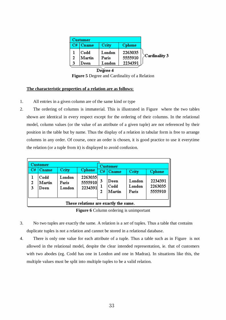
Figure 5 Degree and Cardinality of a Relation
The characteristic properties of a relation are as follows:
1. All entries in a given column are of the same kind or type
2. The ordering of columns is immaterial. This is illustrated in Figure where the two tables
shown are identical in every respect except for the ordering of their columns. In the relational
model, column values (or the value of an attribute of a given tuple) are not referenced by their
position in the table but by name. Thus the display of a relation in tabular form is free to arrange
columns in any order. Of course, once an order is chosen, it is good practice to use it everytime
the relation (or a tuple from it) is displayed to avoid confusion.
Figure 6 Column ordering is unimportant
3. No two tuples are exactly the same. A relation is a set of tuples. Thus a table that contains
duplicate tuples is not a relation and cannot be stored in a relational database.
4. There is only one value for each attribute of a tuple. Thus a table such as in Figure is not
allowed in the relational model, despite the clear intended representation, ie. that of customers
with two abodes (eg. Codd has one in London and one in Madras). In situations like this, the
multiple values must be split into multiple tuples to be a valid relation.
33

Figure 7 A tuple attribute may only have one value
5. The ordering of tuples is immaterial. This follows directly from defining a relation as a set of
tuples, rather than a sequence or list. One is free therefore to display a relation in any convenient
way, eg. sorted on some attribute.
The extension of a relation refers to the current set of tuples in it (see Figure ). This will of
course vary with time as the database changes, ie. as we insert new tuples, or modify or delete
existing ones. Such changes are effected through a DML, or put another way, a DML operates on
the extensions of relations.
The more permanent parts of a relation, viz. the relation name and attribute names, are
collectively referred to as its intension or schema. A relation‟s schema effectively describes (and
constrains) the structure of tuples it is permitted to contain. DML operations on tuples are
allowed only if they observe the expressed intensions of the affected relations (this partially
addresses database integrity concerns raised in the last chapter). Any given database will have a
database schema which records the intensions of every relation in it. Schemas are defined using a
DDL.
Figure 8 The Intension and Extension of a Relation
34

Keys of a Relation
A key is a part of a tuple (one or more attributes) that uniquely distinguishes it from other tuples
in a given relation. Of course, in the extreme, the entire tuple is the key since each tuple in the
relation is guaranteed to be unique. However, we are interested in smaller keys if they exist, for a
number of practical reasons. First, keys will typically be used as links, ie. key values will appear
in other relations to represent their associated tuples (as in Figure above). Thus keys should be
as small as possible and comprise only non redundant attributes to avoid unnecessary duplication
of data across relations. Second, keys form the basis for constructing indexes to speed up
retrieval of tuples from a relation. Small keys will decrease the size of indexes and the time to
look up an index.
Consider Figure below. The customer number (C#) attribute is clearly designed to uniquely
identify a customer. Thus we would not find two or more tuples in the relation having the same
customer number and it can therefore serve as a unique key to tuples in the relation. However,
there may be more than one such key in any relation, and these keys may arise from natural
attributes of the entity represented (rather than a contrived one, like customer number).
Examining again Figure , no two or more tuples have the same value combination of Ccity and
Cphone. If we can safely assume that no customer will share a residence and phone number with
any other customer, then this combination is one such key. Note that Cphone alone is not - there
are two tuples with the same Cphone value (telephone numbers in different cities that happen to
be the same). And neither is Ccity alone as we may expect many customers to live in a given
city.
Figure 9 Candidate Keys
While a relation may have two or more candidate keys, one must be selected and designated as
the primary key in the database schema. For the example above, C# is the obvious choice as a
primary key for the reasons stated earlier. When the primary key values of one relation appear in
35

other relations, they are termed foreign keys. Note that foreign keys may have duplicate
occurrences in a relation, while primary keys may not. For example, in Figure , the C# in
Transaction is a foreign key and the key value „1‟ occurs in two different tuples. This is allowed
because a foreign key is only a reference to a tuple in another relation, unlike a primary key
value, which must uniquely identify a tuple in the relation.
Relational Schema
A Relational Database Schema comprises
1. the definition of all domains
2. the definition of all relations, specifying for each
a) its intension (all attribute names), and
b) a primary key
Figure 10 shows an example of such a schema which has all the components mentioned above.
The primary keys are designated by shading the component attribute names. Of course, this is
only an informal view of a schema. Its formal definition must rely on the use of a specific DDL
whose syntax may vary from one DBMS to another.
Figure 10 An Example Relational Schema
There is, however, a useful notation for relational schemas commonly adopted to document and
communicate database designs free of any specific DDL. It takes the simple form:
<relation name>: <list of attribute names>
Additionally, attributes that are part of the primary key are underlined.
Thus, for the example in Figure , the schema would be written as follows:
36
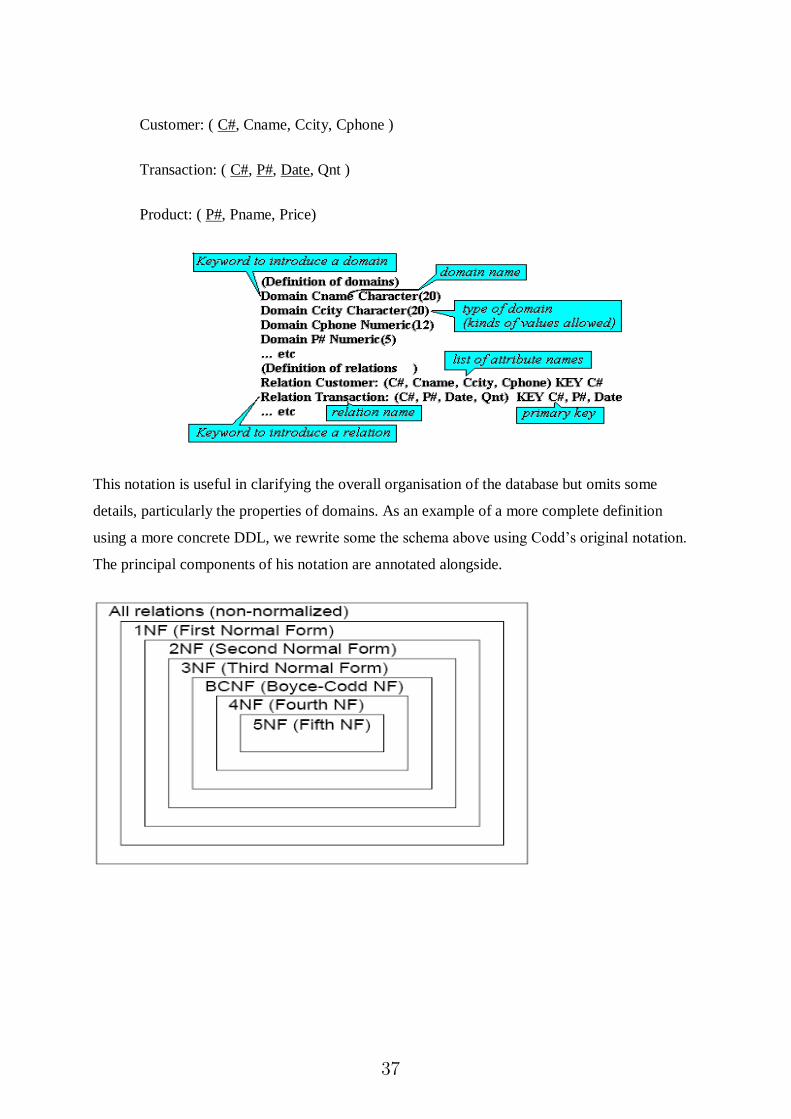
Customer: ( C#, Cname, Ccity, Cphone )
Transaction: ( C#, P#, Date, Qnt )
Product: ( P#, Pname, Price)
This notation is useful in clarifying the overall organisation of the database but omits some
details, particularly the properties of domains. As an example of a more complete definition
using a more concrete DDL, we rewrite some the schema above using Codd‟s original notation.
The principal components of his notation are annotated alongside.
37

Functional Dependencies Definition
Functional dependency (FD) is a constraint between two sets of attributes from the database.
o A functional dependency is a property of the semantics or meaning of the attributes. In every relation
R(A1, A2,…, An) there is a FD called the PK -> A1, A2, …, An Formally the FD is defined as follows
o If X and Y are two sets of attributes, that are subsets of T
For any two tuples t1 and t2 in r , if t1[X]=t2[X], we must also have t1[Y]=t2[Y].
Notation:
o If the values of Y are determined by the values of X, then it is denoted by X -> Y
o Given the value of one attribute, we can determine the value of another attribute
X f.d. Y or X -> y
Example: Consider the following,
Student Number -> Address, Faculty Number -> Department,
Department Code -> Head of Dept
Functional dependencies allow us to express constraints that cannot be expressed using super keys.
Consider the schema:
Loan-info-schema = (customer-name, loan-number,
branch-name, amount).
We expect this set of functional dependencies to hold:
loan-number amount
loan-number branch-name
but would not expect the following to hold:
loan-number customer-name
38
Use of Functional Dependencies
We use functional dependencies to:
o test relations to see if they are legal under a given set of functional dependencies.
o If a relation r is legal under a set F of functional dependencies, we say that r satisfies F.
o specify constraints on the set of legal relations
o We say that F holds on R if all legal relations on R satisfy the set of functional dependencies F.
Note: A specific instance of a relation schema may satisfy a functional dependency even if the
functional dependency does not hold on all legal instances.
o For example, a specific instance of Loan-schema may, by chance, satisfy loan-number customer-
name.
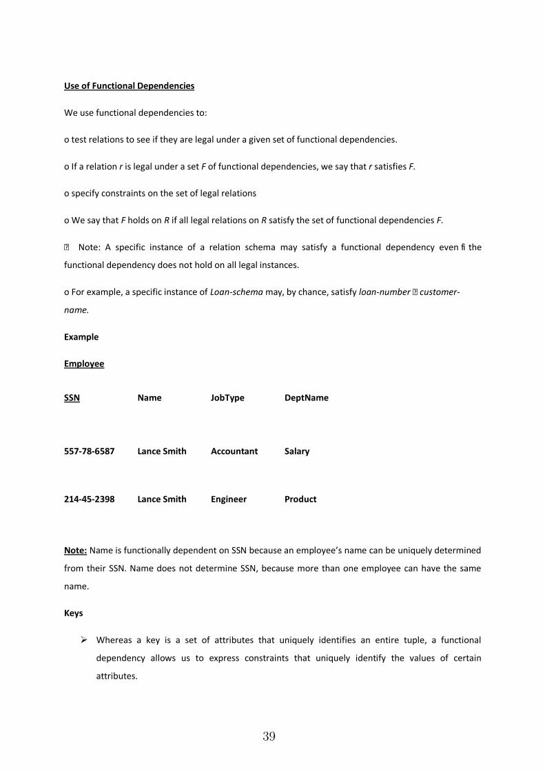
Example
Employee
SSN Name JobType DeptName
557-78-6587 Lance Smith Accountant Salary
214-45-2398 Lance Smith Engineer Product
Note: Name is functionally dependent on SSN because an employee’s name can be uniquely determined
from their SSN. Name does not determine SSN, because more than one employee can have the same
name.
Keys
Whereas a key is a set of attributes that uniquely identifies an entire tuple, a functional
dependency allows us to express constraints that uniquely identify the values of certain
attributes.
39

However, a candidate key is always a determinant, but a determinant doesn’t need to be a key.
Axioms
Before we can determine the closure of the relation, Student, we need a set of rules.
Developed by Armstrong in 1974, there are six rules (axioms) that all possible functional
dependencies may be derived from them.
Axioms Cont.
1. Reflexivity Rule --- If X is a set of attributes and Y is a subset of X, then X Y holds. each subset of X
is functionally dependent on X.
2. Augmentation Rule --- If X Y holds and W is a set of attributes, and then WX WY holds.
3. Transitivity Rule --- If X Y and Y Z holds, then X Z holds.
Derived Theorems from Axioms
4. Union Rule --- If X Y and X Z holds, then X YZ holds.
5. Decomposition Rule --- If X YZ holds, then so do X Y and X Z.
6. Pseudo transitivity Rule --- If X Y and WY Z hold then so does WX Z.
Back to the Example
SNo SName CNo CName Addr Instr. Office
Based on the rules provided, the following dependencies can be derived.
(SNo, CNo) SNo (Rule 1) -- subset
(SNo, CNo) CNo (Rule 1)
(SNo, CNo) (SName, CName) (Rule 2) -- augmentation
CNo office (Rule 3) -- transitivity
SNo (SName, address) (Union Rule) etc.
Properties of FDs
40

X Y says redundant X-values always cause the redundancy of Y-values.
FDs are given by DBAs or DB designers.
FDs are enforced/guaranteed by DBMS.
Given an instance r of a relation R, we can only determine that some FD is not satisfied by R, but
can not determine if an FD is satisfied by R.
Database Normalization
Database normalization is the process of removing redundant data from your tables in to
improve storage efficiency, data integrity, and scalability.
In the relational model, methods exist for quantifying how efficient a database is. These
classifications are called normal forms (or NF), and there are algorithms for converting a given
database between them.
Normalization generally involves splitting existing tables into multiple ones, which must be re-
joined or linked each time a query is issued.
Levels of Normalization
• Levels of normalization based on the amount of redundancy in the database.
• Various levels of normalization are:
– First Normal Form (1NF)
– Second Normal Form (2NF)
– Third Normal Form (3NF)
– Boyce-Codd Normal Form (BCNF)
– Fourth Normal Form (4NF)
– Fifth Normal Form (5NF)
– Domain Key Normal Form (DKNF)
Most databases should be 3NF or BCNF in order to avoid the database anomalies.
Data Anomalies
41
Data anomalies are inconsistencies in the data stored in a database as a result of an operation
such as update, insertion, and/or deletion.
Such inconsistencies may arise when have a particular record stored in multiple locations and
not all of the copies are updated.
We can prevent such anomalies by implementing 7 different level of normalization called
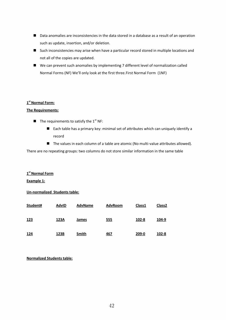
Normal Forms (NF) We’ll only look at the first three.First Normal Form (1NF)
1st Normal Form:
The Requirements:
The requirements to satisfy the 1st NF:
Each table has a primary key: minimal set of attributes which can uniquely identify a
record
The values in each column of a table are atomic (No multi-value attributes allowed).
There are no repeating groups: two columns do not store similar information in the same table
1st Normal Form
Example 1:
Un-normalized Students table:
Student# AdvID AdvName AdvRoom Class1 Class2
123 123A James 555 102-8 104-9
124 123B Smith 467 209-0 102-8
Normalized Students table:
42

Student# AdvID AdvName AdvRoom Class#
123 123A James 555 102-8
123 123A James 555 104-9
124 123B Smith 467 209-0
124 123B Smith 467 102-8
Example 2:
Table 1 problems
This table is not very efficient with storage.
This design does not protect data integrity.
Third, this table does not scale well.
In our Table 1, we have two violations of First Normal Form:
First, we have more than one author field,
Second, our subject field contains more than one piece of information. With more than one
value in a single field, it would be very difficult to search for all books on a given subject.
Title Author1 Author2 ISBN Subject Pages Publisher
Database
System
Concepts
Abraham
Silberschatz
Henry F.
Korth
0072958863 MySQL,
Computers
1168 McGraw-
Hill
Operating
System
Concepts
Abraham
Silberschatz
Henry F.
Korth
0471694665 Computers 944 McGraw-
Hill
43
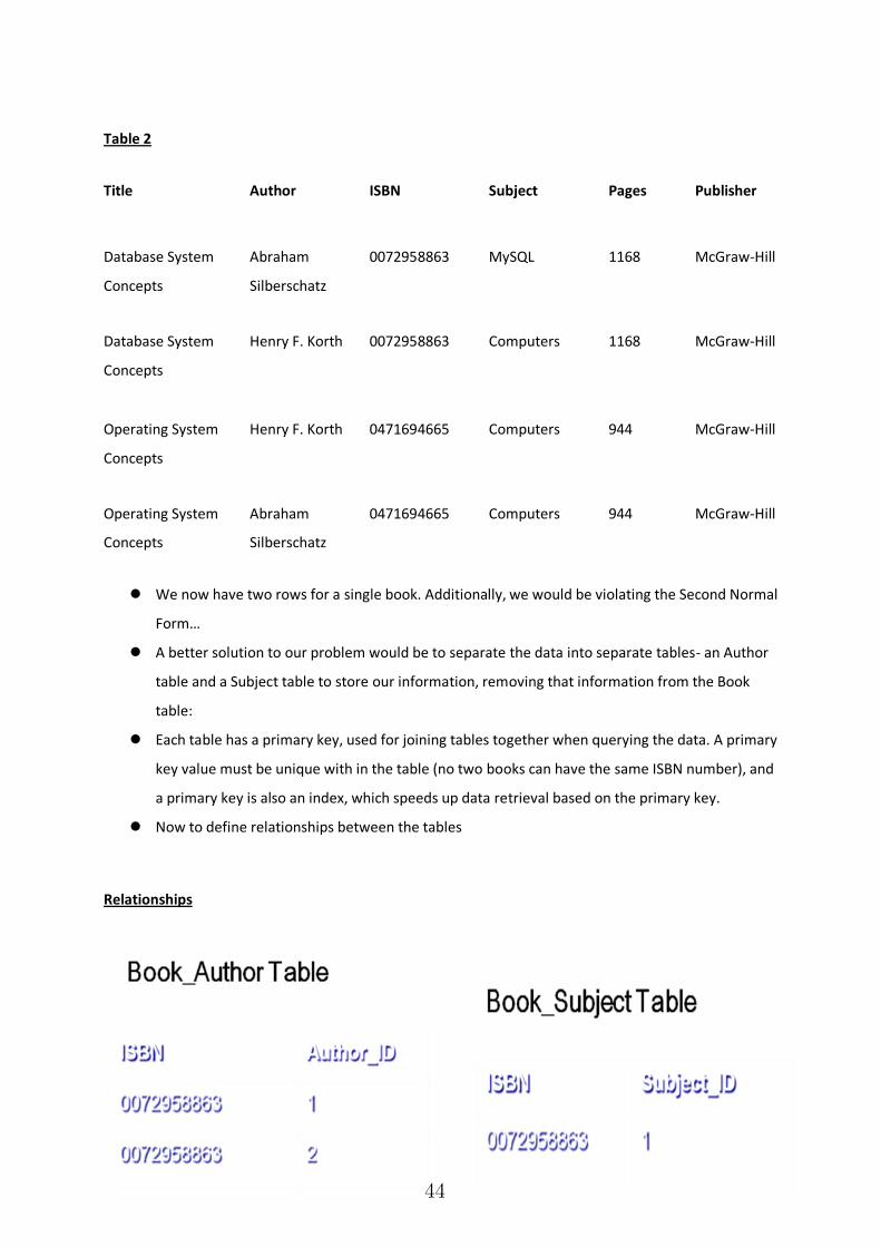
Table 2
Title Author ISBN Subject Pages Publisher
Database System
Concepts
Abraham
Silberschatz
0072958863 MySQL 1168 McGraw-Hill
Database System
Concepts
Henry F. Korth 0072958863 Computers 1168 McGraw-Hill
Operating System
Concepts
Henry F. Korth 0471694665 Computers 944 McGraw-Hill
Operating System
Concepts
Abraham
Silberschatz
0471694665 Computers 944 McGraw-Hill
We now have two rows for a single book. Additionally, we would be violating the Second Normal
Form…
A better solution to our problem would be to separate the data into separate tables- an Author
table and a Subject table to store our information, removing that information from the Book
table:
Each table has a primary key, used for joining tables together when querying the data. A primary
key value must be unique with in the table (no two books can have the same ISBN number), and
a primary key is also an index, which speeds up data retrieval based on the primary key.
Now to define relationships between the tables
Relationships
44

Second Normal Form (2NF)
• a form is in 2NF if and only if it is in 1NF and has no attributes which require only part of the key
to uniquely identify them
• To do - remove part-key dependencies:
1. where a key has more than one attribute, check that each non-key attribute depends on
the whole key and not part of the key
2. for each subset of the key which determines an attribute or group of attributes create a
new form. Move the dependant attributes to the new form.
3. Add the part key to new form, making it the primary key.
4. Mark the part key as a foreign key in the original form.
• Result: 2NF forms
If each attribute A in a relation schema R meets one of the following criteria:
It must be in first normal form.
It is not partially dependent on a candidate key.
Every non-key attribute is fully dependent on each candidate key of the relation.
Second Normal Form (or 2NF) deals with redundancy of data in vertical columns.
Example of Second Normal Form:
Here is a list of attributes in a table that is in First Normal Form:
Department
Project_Name
Employee_Name
Emp_Hire_Date
Project_Manager
Project_Name and Employee_Name are the candidate key for this table. Emp_Hire_Date and
Project_Manager are partially depend on the Employee_Name, but not depend on the Project_Name.
Therefore, this table will not satisfy the Second Normal Form
45

In order to satisfy the Second Normal Form, we need to put the
Emp_Hire_Date and Project_Manager to other tables. We can
put the Emp_Hire_Date to the Employee table and put the
Project_Manager to the Project table.
So now we have three tables:
Department Project
Project_Name Project_ID
Employee_Name Project_Name
Project_Manager
Employee
Employee_ID
Employee_Name
Employee_Hire_Date
Now, the Department table will only have the candidate key left.
Third Normal Form
A relation R is in Third Normal Form (3NF) if and only if it is:
in Second Normal Form.
Every non-key attribute is non-transitively dependent on the primary key.
An attribute C is transitively dependent on attribute A if there exists an attribute B such that A B and
B C, then A C.
46
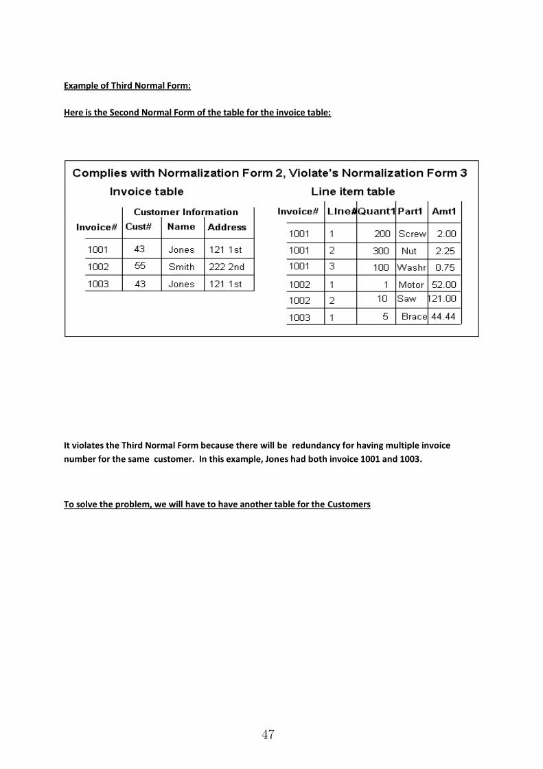
Example of Third Normal Form:
Here is the Second Normal Form of the table for the invoice table:
It violates the Third Normal Form because there will be redundancy for having multiple invoice
number for the same customer. In this example, Jones had both invoice 1001 and 1003.
To solve the problem, we will have to have another table for the Customers
47

By having Customer table, there will be no transitive relationship between the invoice number and
the customer name and address. Also, there will not be redundancy on the customer information
There will be more examples for the First, Second, and Third Normal Forms.
The following is the example of a table that change from each of the normal forms.
Third Normal Form:
Functional Dependency of the Second Normal Form:
SUPPLIER.s# —> SUPPLIER.status (Transitive dependency)
SUPPLIER.s# —> SUPPLIER.city
SUPPLIER.city —> SUPPLIER.status
48

Dependency Preservation:
A FD X! Y is preserved in a relation R if R contains all the attributes of X and Y.
Why Do We Preserve The Dependency?
We would like to check easily that updates to the database do not result in illegal relations being
created.
It would be nice if our design allowed us to check updates without having to compute natural
joins.
Definition
A decomposition D = {R1, R2, ..., Rn} of R is dependency-preserving with respect to F if the union
of the projections of F on each Ri in D is equivalent to F; that is
if (F1 F2 … Fn )+ = F +
Property of Dependency-Preservation
If decomposition is not dependency-preserving, therefore, that dependency is lost in the
decomposition.
Example:
49

R(A B C D)
FD1: A B
FD2: B C
FD3: C D
Decomposition:
R1(A B C) R2(C D)
FD1: A B
FD2: B C
FD3: C D
FD1: A B
FD2: B C
FD3: C D
FD1: A B
50
FD2: B C
FD3: C D
Have all 3 functional dependencies! Therefore, it’s preserving the dependencies
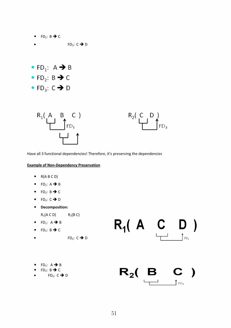
Example of Non-Dependency Preservation
R(A B C D)
FD1: A B
FD2: B C
FD3: C D
Decomposition:
R1(A C D) R2(B C)
FD1: A B
FD2: B C
FD3: C D
FD1: A B FD2: B C
FD3: C D
51

Boyce-Codd Normal Form:
• A relation is in Boyce-Codd normal form (BCNF) if for every FD A B either
• B is contained in A (the FD is trivial), or
• A contains a candidate key of the relation,
• In other words: every determinant in a non-trivial dependency is a (super) key.
• The same as 3NF except in 3NF we only worry about non-key Bs
• If there is only one candidate key then 3NF and BCNF are the same
Stream and BCNF
• Stream is not in BCNF as the FD {Time} {Course} is non-trivial and {Time} does not contain a
candidate key
52
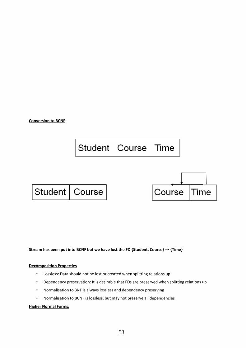
Conversion to BCNF
Stream has been put into BCNF but we have lost the FD {Student, Course} {Time}
Decomposition Properties
• Lossless: Data should not be lost or created when splitting relations up
• Dependency preservation: It is desirable that FDs are preserved when splitting relations up
• Normalisation to 3NF is always lossless and dependency preserving
• Normalisation to BCNF is lossless, but may not preserve all dependencies
Higher Normal Forms:
53

Converting to BCNF
1. The determinant, Offering#, becomes part of the key and the dependant attribute T_Code, becomes a non key attribute. So the Dependency diagram is now
S_Num, Offering# T_Code, Review Date
2. There are problems with this structure as T_Code is now dependant on only part of the key. This violates the rules for 2NF, so the table needs to be divided with the partial dependency becoming a new table. The dependencies would then be
S_Num, Offering# T_Code, Review Date
Offering# T_Code. 3. The original table is divided into two new tables. Each is in 3NF and in BCNF.
Student Review:
S_num Offering# Review Date
123599 01764 2nd
march
123599 01765 12th april
123599 01789 2nd
may
246700 01764 3rd
march
346700 01765 7th may
OfferingTeacher:
Offering# T_code#
54

01764 FIT104
01765 PIT305
01789 PIT107
Note that even relations in BCNF can have anomalies.
Anomalies:
INSERT: We cannot record the city for a supplier_no without also knowing the supplier_name
DELETE: If we delete the row for a given supplier_name, we lose the information that the
supplier_no is associated with a given city.
UPDATE: Since supplier_name is a candidate key (unique), there are none.
Definition of MVD
A multivalued dependency is a full constraint between two sets of attributes in a relation.
In contrast to the functional independency, the multivalued dependency requires that certain tuples be
present in a relation. Therefore, a multivalued dependency is also referred as a tuple-generating
dependency. The multivalued dependency also plays a role in 4NF normalization.
Full constraint
A constraint which expresses something about all attributes in a database. (In contrary to an
embedded constraint.) That a multivalued dependency is a full constraint follows from its
definition, where it says something about the attributes R − β.
Tuple-generating dependency
A dependency which explicitly requires certain tuples to be present in the relation.
A Formal Definition
Let R be a relation schema and let and . The multivalued
dependency α ->> β holds on R if, in any legal relation r(R), for all pairs of tuples t1 and
t2 in r such that t1*α+ = t2*α+, there exist tuples t3 and t4 in r such that
t1*α+ = t2*α+ = t3*α+ = t4*α+
t3*β+ = t1*β+
55

t3[R − β+ = t2[R − β+
t4*β+ = t2*β+
t4[R − β+ = t1[R − β+
A multivalued dependency on R, X ->>Y, says that if two tuples of R agree on all the attributes of X,
then their components in Y may be swapped, and the result will be two tuples that are also in the
relation.
i.e., for each value of X, the values of Y are independent of the values of R-X-Y
Tuples Implied by name->->phones
If we have tuples:
Example
56

But we cannot swap area codes or phones by themselves. That is, neither name->->areaCode nor name-
>->phone holds for this relation.
Properties of MVD
f α ->> β, Then α ->> R − β
If α ->> β and δ γ , Then αδ ->> βγ
If α ->> β and If β ->> γ, then α ->> γ - β
The following also involve functional dependencies:
If α ->> β , then α ->> β
If α -> β and β -> γ, then α -> γ – β
A decomposition of R into (X, Y) and (X, R-Y) is a lossless-join decomposition if and only if X ->> Y
holds in R.
57
MVD Rules
• Every FD is an MVD
– If X ‐>Y, then swapping Y ’s between two tuples that agree on X doesn’t change the tuples.
– Therefore, the “new” tuples are surely in the relation, and we know X ‐>‐>Y.
• Definition of keys depend on FDs and not MDs.
Requires that other tuples of a certain form be present in the relation.
Also referred to as:
“Tuple-generating dependency”
We can use multivalued dependencies
To test relations to determine whether they are legal under a given set of functional and
multivalued dependencies
To specify constraints on the set of legal relations.
4th Normal Form
A Boyce Codd normal form relation is in fourth normal form if
there is no multi value dependency in the relation or
there are multi value dependency but the attributes, which are multi value dependent on a specific
attribute, are dependent between themselves.
This is best discussed through mathematical notation.
Assume the following relation
(a) R(a:pk1, b:pk2, c:pk3)
Recall that a relation is in BCNF if all its determinant are candidate keys, in other words each
determinant can be used as a primary key.
Because relation R has only one determinant (a, b, c), which is the composite primary key and since the
primary is a candidate key therefore R is in BCNF.
Now R may or may not be in fourth normal form.
If R contains no multi value dependency then R will be in Fourth normal form.
Assume R has the following two-multi value dependencies:
a --->> b and a --->> c
58

In this case R will be in the fourth normal form if b and c dependent on each other.
However if b and c are independent of each other then R is not in fourth normal form and the relation
has to be projected to following two non-loss projections. These non-loss projections will be in fourth
normal form.
Many-to-many relationships
Fourth Normal Form applies to situations involving many-to-many relationships.
In relational databases, many-to-many relationships are expressed through cross-reference tables.
Note about FDs and MVDs
Every Functional Dependency is a MVD
(if A1A2…An ® B1B2…Bn , then A1A2…An Þ B1B2…Bn )
FDs rule out certain tuples (i.e. if A ® B then two tuples will not have the same value for A and different
values for B)
MVDs do not rule out tuples. They guarantee that certain tuples must exist.
4th NF and Anomalies
As an example of the anomalies that can occur, realize that it is not possible to add a new class taught
by some teacher without adding at least one student who is enrolled in this class.
To achieve 4NF, represent each independent many-to-many relationship through its own cross-
reference table.
Case 1:
Assume the following relation:
Employee (Eid:pk1, Language:pk2, Skill:pk3)
No multi value dependency, therefore R is in fourth normal form.
Case 2:
Assume the following relation with multi-value dependency:
Employee (Eid:pk1, Languages:pk2, Skills:pk3)
Eid --->> Languages Eid --->> Skills
59

Languages and Skills are dependent.
This says an employee speak several languages and has several skills. However for each
skill a specific language is used when that skill is practiced
Thus employee 100 when he/she teaches speaks English but when he cooks speaks
French. This relation is in fourth normal form and does not suffer from any anomalies.
Eid Language Skill
100 English Teaching
100 Kurdish Politic
100 French Cooking
200 English Cooking
200 Arabic Singing
Case 3:
Assume the following relation with multi-value dependency:
Employee (Eid:pk1, Languages:pk2, Skills:pk3)
Eid --->> Languages Eid --->> Skills
Languages and Skills are independent.
This relation is not in fourth normal form and suffers from all three types of anomalies.
60

Eid Language Skill
100 English Teaching
100 Kurdish Politic
100 English Politic
100 Kurdish Teaching
200 Arabic Singing
Insertion anomaly: To insert row (200 English Cooking) we have to insert two extra rows (200 Arabic
cooking), and (200 English Singing) otherwise the database will be inconsistent. Note the table will be as
follow:
Eid Language Skill
100 English Teaching
100 Kurdish Politics
100 English Politics
100 Kurdish Teaching
200 Arabic Singing
200 English Cooking
200 Arabic Cooking
200 English Singing
61
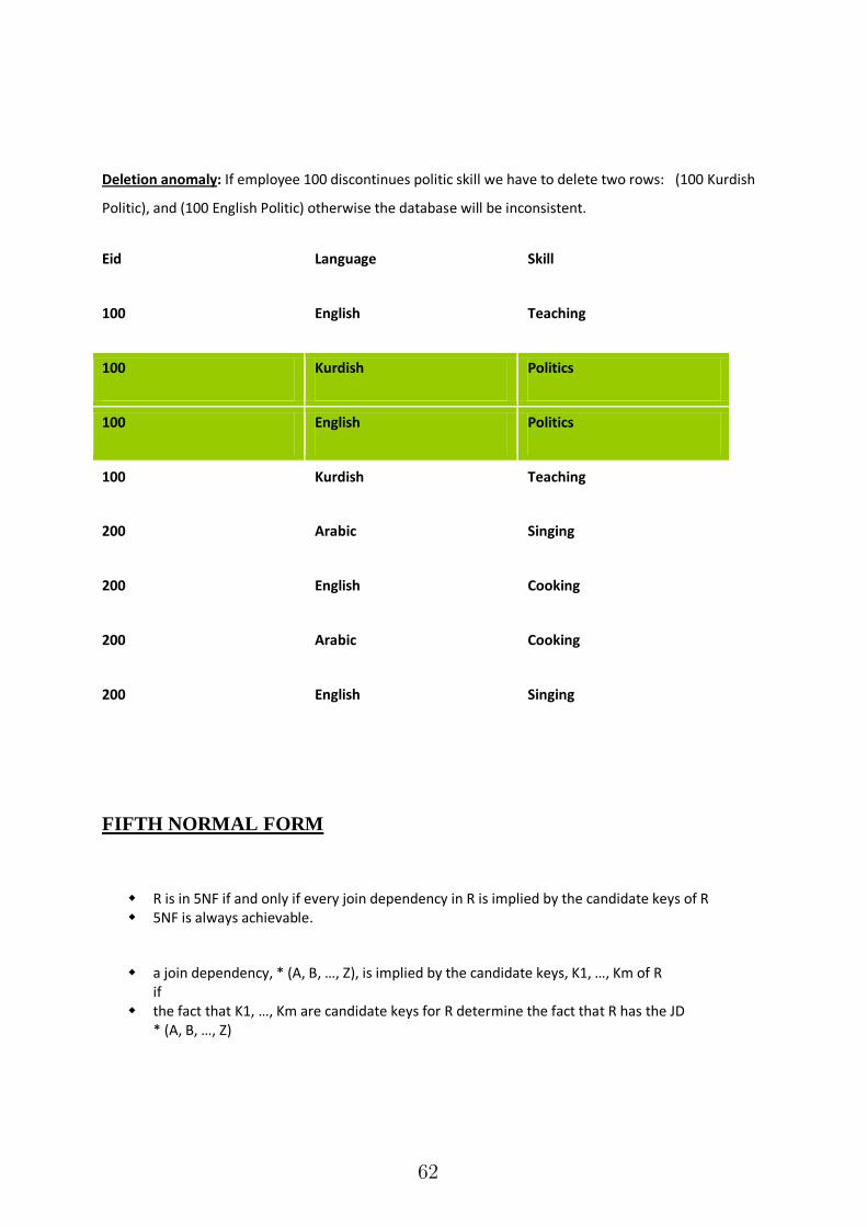
Deletion anomaly: If employee 100 discontinues politic skill we have to delete two rows: (100 Kurdish
Politic), and (100 English Politic) otherwise the database will be inconsistent.
Eid Language Skill
100 English Teaching
100 Kurdish Politics
100 English Politics
100 Kurdish Teaching
200 Arabic Singing
200 English Cooking
200 Arabic Cooking
200 English Singing
FIFTH NORMAL FORM
R is in 5NF if and only if every join dependency in R is implied by the candidate keys of R 5NF is always achievable.
a join dependency, * (A, B, …, Z), is implied by the candidate keys, K1, …, Km of R if the fact that K1, …, Km are candidate keys for R determine the fact that R has the JD
* (A, B, …, Z)
62

63

Problems in bringing a relation to 5NF
check whether all JDs are implied by the candidate keys
Fagin : provides an algorithm for doing this for any relation, given all its JDs and
all candidate keys
discover all JDs for a given relation
they do not have that intuitive meaning as FDs or MVDs
A relation is in 5NF if every join dependency in the relation is implied by the keys of the relation
Implies that relations that have been decomposed in previous normal forms can be recombined
via natural joins to recreate the original relation.
Usage
Only in rare situations does a 4NF table not conform to 5NF. These are situations in
which a complex real-world constraint governing the valid combinations of attribute values in
the 4NF table is not implicit in the structure of that table. If such a table is not normalized to
5NF, the burden of maintaining the logical consistency of the data within the table must be
carried partly by the application responsible for insertions, deletions, and updates to it; and there
is a heightened risk that the data within the table will become inconsistent. In contrast, the 5NF
design excludes the possibility of such inconsistencies.
Example 2:
Consider a relation Supply (sname, partName, projName). Add the additional constraint that:
If project j requires part p
and supplier s supplies part p
and supplier s supplies at least one item to project j Then
supplier s also supplies part p to project j
64

Let R be in BCNF and let R have no composite keys. Then R is in 5NF
Note: That only joining all three relations together will get you back to the original relation. Joining any
two will create spurious tuples!
65

66

UNIT II SQL & QUERY OPTIMIZATION 8
SQL Standards - Data types - Database Objects- DDL-DML-DCL-TCL-Embedded SQL-Static
Vs Dynamic SQL - QUERY OPTIMIZATION: Query Processing and Optimization -
Heuristics and Cost Estimates in Query Optimization.
Textbook:
Ramez Elmasri and Shamkant B. Navathe, ―Fundamentals of Database Systems‖, Fifth
Edition, Pearson Education, 2008.
SQL Overview
Structured Query Language
The standard for relational database management systems (RDBMS)
SQL-92 and SQL-99 Standards – Purpose:
Specify syntax/semantics for data definition and manipulation
Define data structures
Enable portability
Specify minimal (level 1) and complete (level 2) standards
Allow for later growth/enhancement to standard
Catalog
A set of schemas that constitute the description of a database
Schema
The structure that contains descriptions of objects created by a user (base tables, views,
constraints)
Data Definition Language (DDL)
Commands that define a database, including creating, altering, and dropping tables and
establishing constraints
Data Manipulation Language (DML)
Commands that maintain and query a database
Data Control Language (DCL)
Commands that control a database, including administering privileges and committing
data 67
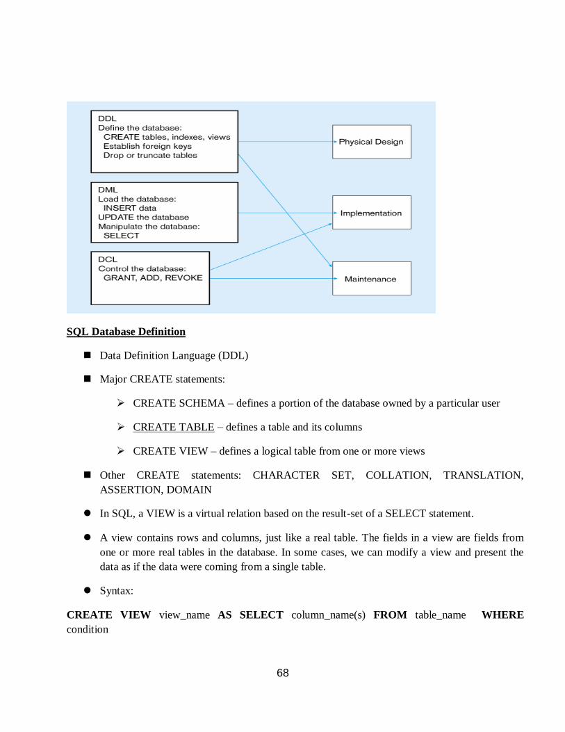
SQL Database Definition
Data Definition Language (DDL)
Major CREATE statements:
CREATE SCHEMA – defines a portion of the database owned by a particular user
CREATE TABLE – defines a table and its columns
CREATE VIEW – defines a logical table from one or more views
Other CREATE statements: CHARACTER SET, COLLATION, TRANSLATION,
ASSERTION, DOMAIN
In SQL, a VIEW is a virtual relation based on the result-set of a SELECT statement.
A view contains rows and columns, just like a real table. The fields in a view are fields from
one or more real tables in the database. In some cases, we can modify a view and present the
data as if the data were coming from a single table.
Syntax:
CREATE VIEW view_name AS SELECT column_name(s) FROM table_name WHERE
condition
68

SQL – Relations, Tables & Views
When we say Relation, it could be a Table or a View. There are three kind of relations:
1. Stored relations tables
We sometimes use the term ―base relation‖ or ―base table‖
1. Virtual relations views
2. Temporary results
SQL – Create View
Example: Create a view with title and year and made by Paramount studio. Movie (title, year,
length, inColor, studioName, producerC#)
CREATE VIEW ParamountMovie AS SELECT title,year FROM Movie WHERE studioName =
‗Paramount‘;
SQL – Querying View
A view could be used from inside a query, a stored procedure, or from inside another view. By
adding functions, joins, etc., to a view, it allows us to present exactly the data we want to the
user.
SELECT title FROM ParamountMovie WHERE year = ‗1979‘;
Have same result as
SELECT title FROM Movie WHERE studioName = ‗Paramount‘ AND year = ‗1979‘;
Example:
Movie (title, year, length, inColor, studioName, producerC#) MovieExec (name, address, cert#,
netWorth)
CREATE VIEW MovieProd AS SELECT title, name FROM Movie, MovieExec WHERE
producerC# = cert#; SELECT name FROM MovieProd WHERE title = ‗Gone With the Wind‘;
Same result as query from tables
SELECT name FROM Movie, MovieExec WHERE producerC# = cert# AND title = ‗The War Of
the World‘;
Data Types in SQL
69

String types
CHAR(n) – fixed-length character data, n characters long Maximum length = 2000
bytes
VARCHAR2(n) – variable length character data, maximum 4000 bytes
LONG – variable-length character data, up to 4GB. Maximum 1 per table
Numeric types
NUMBER(p,q) – general purpose numeric data type
INTEGER(p) – signed integer, p digits wide
FLOAT(p) – floating point in scientific notation with p binary digits precision
Date/time type
DATE – fixed-length date/time in dd-mm-yy form
70
An object database (also object-oriented database management system) is a database
management system in which information is represented in the form of objects as used in object-
oriented programming. Object databases are different from relational databases which are table-
oriented. Object-relational databases are a hybrid of both approaches.
Object-oriented database management systems (OODBMSs) combine database capabilities
with object-oriented programming language capabilities. OODBMSs allow object-oriented
programmers to develop the product, store them as objects, and replicate or modify existing objects to
make new objects within the OODBMS. Because the database is integrated with the programming
language, the programmer can maintain consistency within one environment, in that both the
OODBMS and the programming language will use the same model of representation. Relational
DBMS projects, by way of contrast, maintain a clearer division between the database model and the
application.
class Dbms( )
Creates a Dbms object. Dbms objects support basic operations on a database.
Dbms objects have the following methods:
begin( )
Begins a transaction on the database.
close( )
Closes the database object. It is safe to try to close a database object even if it is not open.
commit( )
Commits the current transaction. 71

compact( )
Compacts the database, reclaiming unused space in the database file.
create( dbname)
Creates a database with path dbname.
execute( query)
Executes an SQL query. On success, returns 0 if a DDL (SQL schema update) statement was
executed. Returns the number of rows inserted, updated, or deleted, if a DML (SQL data
update) statement was executed.
open( dbname)
Opens the database in file dbname. This should be a full Unicode path name, for example,
u'c:\\foo.db'.
rollback( )
Rolls back the current transaction.
Data Definition Language:
A data definition language or data description language (DDL) is a syntax similar to a
computer programming language for defining data structures, especially database schemas. Many data
description languages use a declarative syntax to define fields and data types. SQL, however, uses a
collection of imperative verbs whose effect is to modify the schema of the database by adding,
changing, or deleting definitions of tables or other objects. These statements can be freely mixed with
other SQL statements, so the DDL is not truly a separate language.
CREATE statements
Create - To make a new database, table, index, or stored procedure.
A CREATE statement in SQL creates an object in a relational database management system
(RDBMS). In the SQL 1992 specification, the types of objects that can be created are schemas, tables,
views, domains, character sets, collations, translations, and assertions. Many implementations extend
the syntax to allow creation of additional objects, such as indexes and user profiles. Some systems
(such as PostgreSQL) allow CREATE, and other DDL commands, inside a transaction and thus they
may be rolled back.
CREATE TABLE statement
A commonly used CREATE command is the CREATE TABLE command. The typical usage is:
CREATE TABLE [table name] ( [column definitions] ) [table parameters].
column definitions: A comma-separated list consisting of any of the following
Column definition: [column name] [data type] {NULL | NOT NULL} {column options}
Primary key definition: PRIMARY KEY ( [comma separated column list] )
Constraints: {CONSTRAINT} [constraint definition]
RDBMS specific functionality
For example, the command to create a table named employees with a few sample columns
would be: 72
CREATE TABLE employees (
id INTEGER PRIMARY KEY,
first_name VARCHAR(50) NULL,
last_name VARCHAR(75) NOT NULL,
fname VARCHAR(50) NOT NULL,
dateofbirth DATE NULL
);
DROP statements
Drop - To destroy an existing database, table, index, or view.
A DROP statement in SQL removes an object from a relational database management system
(RDBMS). The types of objects that can be dropped depends on which RDBMS is being used, but
most support the dropping of tables, users, and databases. Some systems (such as PostgreSQL) allow
DROP and other DDL commands to occur inside of a transaction and thus be rolled back.
DROP objecttype objectname.
For example, the command to drop a table named employees would be:
DROP employees;
The DROP statement is distinct from the DELETE and TRUNCATE statements, in that
DELETE and TRUNCATE do not remove the table itself. For example, a DELETE statement might
delete some (or all) data from a table while leaving the table itself in the database, whereas a DROP
statement would remove the entire table from the database.
ALTER statements
Alter - To modify an existing database object.
An ALTER statement in SQL changes the properties of an object inside of a relational database
management system (RDBMS). The types of objects that can be altered depends on which RDBMS is
being used. The typical usage is:
ALTER objecttype objectname parameters.
For example, the command to add (then remove) a column named bubbles for an existing table
named sink would be:
ALTER TABLE sink ADD bubbles INTEGER;
ALTER TABLE sink DROP COLUMN bubbles;
Rename statement
Rename - to rename the table. for example
RENAME TABLE old_name TO new_name; 73

Referential integrity statements
Finally, another kind of DDL sentence in SQL is one used to define referential integrity relationships,
usually implemented as primary key and foreign key tags in some columns of the tables. These two
statements can be included inside a CREATE TABLE or an ALTER TABLE sentence.
Data Manipulation Language (DML)
A data manipulation language (DML) is a family of syntax elements similar to a computer
programming language used for Selecting , inserting, deleting and updating data in a database.
Performing read-only queries of data is sometimes also considered a component of DML.
A popular data manipulation language is that of Structured Query Language (SQL), which is
used to retrieve and manipulate data in a relational database. Other forms of DML are those used by
IMS/DLI, CODASYL databases, such as IDMS and others.
A data manipulation language (DML) is a family of computer languages including commands
permitting users to manipulate data in a database. This manipulation involves inserting data into
database tables, retrieving existing data, deleting data from existing tables and modifying existing
data. DML is mostly incorporated in SQL databases.
Data manipulation language comprises the SQL data change statements, which modify stored
data but not the schema or database objects. Manipulation of persistent database objects, e.g., tables or
stored procedures, via the SQL schema statements, rather than the data stored within them, is
considered to be part of a separate data definition language. In SQL these two categories are similar in
their detailed syntax, data types, expressions etc., but distinct in their overall function.
DML resembles simple English language and enhances efficient user interaction with the system. The
functional capability of DML is organized in manipulation commands like SELECT, UPDATE,
INSERT INTO and DELETE FROM, as described below:
SELECT: This command is used to retrieve rows from a table. The select syntax is SELECT
[column name(s)] from [table name] where [conditions]. Select is the most widely used DML
command in SQL.
UPDATE: This command modifies data of one or more records. An update command syntax is
UPDATE table name SET column name = value where [condition].
INSERT: This command adds one or more records to a database table. The insert command
syntax is INSERT INTO table name [column(s)] VALUES [value(s)].
DELETE: This command removes one or more records from a table according to specified
conditions. Delete command syntax is DELETE FROM table name where [condition]. 74
Data manipulation languages have their functional capability organized by the initial word in a
statement, which is almost always a verb. In the case of SQL, these verbs are:
SELECT ... FROM ... WHERE ...
INSERT INTO ... VALUES ...
UPDATE ... SET ... WHERE ...
DELETE FROM ... WHERE ...
1.Select Command
Syntax
SELECT [DISTINCT|ALL]{*|column|column_expression [AS new_name][,…]}
FROM table_name [alias] [, … ]
[WHERE condition]
[GROUP BY column_list]
[HAVING condition]
[ORDER BY column_list [ASC|DESC]];
column represents a column name.
column_expression represents an expression on a column.
table_name is the name of an existing database table or view.
FROM specifies the table(s) to be used.
WHERE filters the rows subject to some condition.
GROUP BY forms groups of rows with the same column name.
SELECT specifies which column are to appear in the output.
ORDER BY specifies the order of the output.
Order of the clauses in the SELECT statement can not be changed.
The result of a query is another table.
Asterisk (*) means all columns.
Five aggregation functions defined in SQL:
COUNT returns the number of rows in a specified column.
SUM returns the sum of the values in a specified column.
AVG returns the average of the values in a specified column.
MIN returns the smallest value in a specified column.
MAX returns the largest value in a specified column.
75

Examples:
Property (PropertyNo, Street, City, postcode, Type, OwnerNo, Rooms, Rent)
How many properties cost more than 350 per month to rent?
SELECT COUNT(*) AS count FROM property WHERE rent > 350;
Subqueries
A complete SELECT statement can be embedded (subselect) within another SELECT
statement.
A subselect can be used in the WHERE and HAVING clauses of the outer SELECT statement
(nested query).
A subquery can be used immediately following a relational operator.
Subquery always enclosed in parentheses.
Type of subquery: A scalar subquery returns a single column and a single row (singlevalue).
A row subquery returns multiple columns, but a single row.
A table subquery returns one or more columns and multiple rows.
STAFF (sno, fname, lname, position, sex, DOB, salary, bno)
BRANCH (bno, street, city, postcode)
Example:
List the staff who work in the branch at ‗163 Main St‘.
SELECT sno, fname, lname, position FROM staff WHERE bno = (SELECT bno FROM
branch WHERE street = ‗163 Main St‘);
Modifying Data in the DB (UPDATE)
Syntax
UPDATE table_name
SET column_name1 = data_value1 [, column_namei = data_valuei ...]
[WHERE search_condition]
table_name may be either a base table or an updatable view.
The SET clause specifies the names of one or more columns that are updated for
all rows in the table.
Only rows that satisfy the search_condition are updated.
data_values must be compatible with the data types for the corresponding
columns.
Data Control Language
A data control language (DCL) is a syntax similar to a computer programming language used
to control access to data stored in a database. In particular, it is a component of Structured Query
Language (SQL).
76

It is used to create roles, permissions, and referential integrity as well it is used to control
access to database by securing it. These SQL commands are used for providing security to database
objects. These commands are GRANT and REVOKE.
Examples of DCL commands include:
GRANT to allow specified users to perform specified tasks. REVOKE to cancel previously granted or denied permissions.
The Data Control Language (DCL) component of the SQL language is used to create privileges
to allow users access to, and manipulation of, the database. There are two main commands:
GRANT to grant a privilege to a user
REVOKE to revoke (remove) a privilege from a user
The operations for which privileges may be granted to or revoked from a user or role may include
CONNECT, SELECT, INSERT, UPDATE, DELETE, EXECUTE, and USAGE. In the Oracle
database, executing a DCL command issues an implicit commit. Hence you cannot roll back the
command. In PostgreSQL, executing DCL is transactional, and can be rolled back.
SQL GRANT REVOKE Commands
DCL commands are used to enforce database security in a multiple user database environment. Two
types of DCL commands are GRANT and REVOKE. Only Database Administrator's or owner's of the
database object can provide/remove privileges on a database object.
SQL GRANT Command
SQL GRANT is a command used to provide access or privileges on the database objects to the users.
The Syntax for the GRANT command is:
GRANT privilege_name ON object_name TO {user_name |PUBLIC |role_name} [WITH GRANT
OPTION];
privilege_name is the access right or privilege granted to the user. Some of the access rights
are ALL, EXECUTE, and SELECT.
object_name is the name of an database object like TABLE, VIEW, STORED PROC and
SEQUENCE.
user_name is the name of the user to whom an access right is being granted.
user_name is the name of the user to whom an access right is being granted.
PUBLIC is used to grant access rights to all users.
ROLES are a set of privileges grouped together.
WITH GRANT OPTION - allows a user to grant access rights to other users.
For Example: GRANT SELECT ON employee TO user1; This command grants a SELECT
permission on employee table to user1.You should use the WITH GRANT option carefully because 77

for example if you GRANT SELECT privilege on employee table to user1 using the WITH GRANT
option, then user1 can GRANT SELECT privilege on employee table to another user, such as user2
etc. Later, if you REVOKE the SELECT privilege on employee from user1, still user2 will have
SELECT privilege on employee table.
SQL REVOKE Command:
The REVOKE command removes user access rights or privileges to the database objects.
The Syntax for the REVOKE command is:
REVOKE privilege_name ON object_name FROM {user_name |PUBLIC |role_name}
For Example: REVOKE SELECT ON employee FROM user1;This command will REVOKE a
SELECT privilege on employee table from user1.When you REVOKE SELECT privilege on a table
from a user, the user will not be able to SELECT data from that table anymore. However, if the user
has received SELECT privileges on that table from more than one users, he/she can SELECT from
that table until everyone who granted the permission revokes it.
Privileges and Roles:
Privileges: Privileges defines the access rights provided to a user on a database object. There are two
types of privileges.
1) System privileges - This allows the user to CREATE, ALTER, or DROP database objects.
2) Object privileges - This allows the user to EXECUTE, SELECT, INSERT, UPDATE, or DELETE
data from database objects to which the privileges apply.
Few CREATE system privileges are listed below:
System Privileges Description
CREATE object allows users to create the specified object in their
own schema.
CREATE ANY object allows users to create the specified object in any
schema.
The above rules also apply for ALTER and DROP system privileges.
Few of the object privileges are listed below:
Object Privileges Description 78

INSERT allows users to insert rows into a table.
SELECT allows users to select data from a database object.
UPDATE allows user to update data in a table.
EXECUTE allows user to execute a stored procedure or a
function.
Roles: Roles are a collection of privileges or access rights. When there are many users in a database it
becomes difficult to grant or revoke privileges to users. Therefore, if you define roles, you can grant or
revoke privileges to users, thereby automatically granting or revoking privileges. You can either create
Roles or use the system roles pre-defined by oracle.
Some of the privileges granted to the system roles are as given below:
System Role Privileges Granted to the Role
CONNECT CREATE TABLE, CREATE VIEW, CREATE SYNONYM,
CREATE SEQUENCE, CREATE SESSION etc.
RESOURCE
CREATE PROCEDURE, CREATE SEQUENCE, CREATE
TABLE, CREATE TRIGGER etc. The primary usage of
the RESOURCE role is to restrict access to database
objects.
DBA ALL SYSTEM PRIVILEGES
Creating Roles:
The Syntax to create a role is:
CREATE ROLE role_name [IDENTIFIED BY password];
For Example: To create a role called "developer" with password as "pwd",the code will be as follows
CREATE ROLE testing [IDENTIFIED BY pwd];
It's easier to GRANT or REVOKE privileges to the users through a role rather than assigning a
privilege directly to every user. If a role is identified by a password, then, when you GRANT or
REVOKE privileges to the role, you definitely have to identify it with the password.
We can GRANT or REVOKE privilege to a role as below.
For example: To grant CREATE TABLE privilege to a user by creating a testing role: 79
First, create a testing Role
CREATE ROLE testing
Second, grant a CREATE TABLE privilege to the ROLE testing. You can add more privileges to the
ROLE.
GRANT CREATE TABLE TO testing;
Third, grant the role to a user.
GRANT testing TO user1;
To revoke a CREATE TABLE privilege from testing ROLE, you can write:
REVOKE CREATE TABLE FROM testing;
The Syntax to drop a role from the database is as below:
DROP ROLE role_name;
For example: To drop a role called developer, you can write:
DROP ROLE testing;
GRANT command
In order to do anything within an Oracle database you must be given the appropriate privileges. Oracle
operates a closed system in that you cannot perform any action at all unless you have been authorized
to do so. This includes logging onto the database, creating tables, views, indexes and synonyms,
manipulating data (ie select, insert, update and delete) in tables created by other users, etc.
The SQL command to grant a privilege on a table is:
GRANT SELECT, INSERT, UPDATE, DELETE ON tablename TO username;
There are many more forms of the GRANT command, but this is sufficient for this Unit.
Any combination of the above privileges is allowed. You can issue this command on any tables that
you have created. For example:
GRANT SELECT ON employee TO hn23;
GRANT SELECT, UPDATE, DELETE ON employee TO hn44;
REVOKE command
The SQL command to revoke a privilege on a table is:
REVOKE SELECT, INSERT, UPDATE, DELETE ON tablename FROM username; 80

For example:
REVOKE SELECT ON employee FROM hn23;
REVOKE SELECT, UPDATE, DELETE FROM hn44;
Transaction Control Language (TCL)
A Transaction Control Language (TCL) is a computer language and a subset of SQL, used to control
transactional processing in a database. A transaction is logical unit of work that comprises one or more
SQL statements, usually a group of Data Manipulation Language (DML) statements.
A series of one or more SQL statements that are logically related, or a series of operation performed on Oracle table data is termed as a Transaction. Oracle treats changes to table data as a two step process. First the changes requested are done. To make these changes permanent a COMMIT statement has to be given at the SQL prompt. A ROLLBACK statement given at the SQL prompt can be used to undo a part of or the entire Transaction. A Transaction begins with the first executable SQL statement after a Commit, Rollback or Connection made to the Oracle engine. All changes made to an Oracle table data via a transaction are made or undo at one instance. Specially, a Transaction is a group of events that occurs between any of the following events:
Connecting to Oracle
Disconnecting from Oracle
Committing changes to the table
Rollback
TCL is abbreviation of Transactional Control Language. It is used to manage different transactions
occurring within a database.
Examples of TCL commands include:
COMMIT to apply the transaction by saving the database changes.
ROLLBACK to undo all changes of a transaction.
SAVEPOINT to divide the transaction into smaller sections. It defines breakpoints for a
transaction to allow partial rollbacks.
COMMIT
PURPOSE: To end your current transaction and make permanent all changes performed in the
transaction. This command also erases all savepoints in the transaction and releases the transaction's
locks. You can also use this command to manually commit an in-doubt distributed transaction.
SYNTAX:
COMMIT [WORK] [ COMMENT 'text' | FORCE 'text' [, integer] ]
Where: 81

WORK : is supported only for compliance with standard SQL. The statements COMMIT and
COMMIT WORK are equivalent.
COMMENT : specifies a comment to be associated with the current transaction. The 'text' is a
quoted literal of up to 50 characters that Oracle stores in the data dictionary view
DBA_2PC_PENDING along with the transaction ID if the transaction becomes in-doubt.
FORCE : manually commits an in-doubt distributed transaction. The transaction is identified
by the 'text' containing its local or global transaction ID. To find the IDs of such transactions,
query the data dictionary view DBA_2PC_PENDING. You can also use the integer to
specifically assign the transaction a system change number (SCN). If you omit the integer, the
transaction is committed using the current SCN.
COMMIT statements using the FORCE clause are not supported in PL/SQL.
PREREQUISITES:
You need no privileges to commit your current transaction.
To manually commit a distributed in-doubt transaction that you originally committed, you must have
FORCE TRANSACTION system privilege. To manually commit a distributed in-doubt transaction
that was originally committed by another user, you must have FORCE ANY TRANSACTION system
privilege.
Example:
To commit your current transaction, enter
SQL> COMMIT WORK;
Commit complete.
ROLLBACK
PURPOSE:
To undo work done in the current transaction. You can also use this command to manually und the
work done by an in-doubt distributed transaction.
SYNTAX:
ROLLBACK [WORK][ TO [SAVEPOINT] savepoint | FORCE 'text' ]
Where:
WORK : is optional and is provided for ANSI compatibility.
TO : rolls back the current transaction to the specified savepoint. If you omit this clause, the
ROLLBACK statement rolls back the entire transaction.
FORCE : manually rolls back an in-doubt distributed transaction. The transaction is identified
by the 'text' containing its local or global transaction ID. To find the IDs of such transactions,
query the data dictionary view DBA_2PC_PENDING.
ROLLBACK statements with the FORCE clause are not supported in PL/SQL.
PREREQUISITES:
To roll back your current transaction, no privileges are necessary.
To manually roll back an in-doubt distributed transaction that you originally committed, you must 82

have FORCE TRANSACTION system privilege. To manually roll back an in-doubt distributed
transaction originally committed by another user, you must have FORCE ANY TRANSACTION
system privilege.
Example:
To rollback your current transaction, enter
SQL> ROLLBACK;
Rollback complete.
CLOSING TRANSACTION:
A Transaction can be closed by using either a Commit or a Rollback statement. By using these
statement, table data can be changed or all the changes made to the table data undo.
Using COMMIT:
A COMMIT ends the current transaction and makes permanent any changes made during the
transaction. All transaction locks acquired on tables are released.
Syntax:
COMMIT;
Using ROLLBACK:
A ROLLBACK does exactly the opposite of COMMIT. It ends the transaction but undoes any
changes made during the transaction. All transaction locks acquired on tables are released.
Syntax: ROLLBACK [WORK] [TO SAVEPOINT] < Save-point_Name>
WORK: It is optional and is provided for ANSI compatibility
SAVEPOINT : It is optional and it is used to rollback a partial transaction, as far as the
specified savepoint.
SAVEPOINTNAME: It is a savepoint created during the current transaction
Crating a SAVEPOINT:
SAVEPOINT marks and saves the current point in the processing of a transaction. When a
SAVEPOINT is used with a ROLLBACK statement, parts of a transaction can be undone. An active
savepoint is one that is specified since the last COMMIT or ROLLBACK.
Syntax:
SAVEPOINT <SavePointName>
Example:
DECLARE 83

Total_Sal number(9);
BEGIN
INSERT INTO Emp VALUES('E101', 'Aamir', 10, 7000');
INSERT INTO Emp VALUES('E102', 'Aatif', 11, 6500');
SAVEPOINT no_update;
UPDATE Emp SET salary =salary+2000 WHERE Emp_Name = 'Aamir';
UPDATE Emp SET salary =salary+2000 WHERE Emp_Name = 'Aatif';
SELECT sum(Salary) INTO Total_sal FROM Emp;
IF Total_Sal > 15000 THEN
ROLLBACK To SAVEPOINT no_update;
END IF;
COMMIT;
END;
The bove PL/SQL block, it will insert two records in the table Emp, then after no_update SavePoint
has been declared.
on both of record the updated with 2000 respectively, now calculated all the salary in Emp Table, If
Salary has been reached more than 15000 in its table, then it is automatically rolled back, it means
undo that was updated earlier by 2000. If this type situation is coming then you can use these
commands.
Embedded SQL
Embedded SQL is a method of combining the computing power of a programming
language and the database manipulation capabilities of SQL. Embedded SQL statements are SQL
statements written inline with the program source code of the host language. The embedded SQL
statements are parsed by an embedded SQL preprocessor and replaced by host-language calls to a
code library. The output from the preprocessor is then compiled by the host compiler. This allows
programmers to embed SQL statements in programs written in any number of languages such
as: C/C++, COBOL and Fortran.
The SQL standards committee defined the embedded SQL standard in two steps: a formalism called Module Language was defined, then the embedded SQL standard was derived from Module
Language.
Embedded SQL is a robust and convenient method of combining the computing power of a programming language with SQL's specialized data management and manipulation capabilities.
Static Vs Dynamic SQL:
Static SQL
The source form of a static SQL statement is embedded within an application program written in a
host language such as COBOL. 84

The statement is prepared before the program is executed and the operational form of the
statement persists beyond the execution of the program.
Static SQL statements in a source program must be processed before the program is compiled.
This processing can be accomplished through the DB2 precompiler or the SQL statement
coprocessor.
The DB2 precompiler or the coprocessor checks the syntax of the SQL statements, turns them
into host language comments, and generates host language statements to invoke DB2.
The preparation of an SQL application program includes precompilation, the preparation of its
static SQL statements, and compilation of the modified source program.
Dynamic SQL:
Programs that contain embedded dynamic SQL statements must be precompiled
like those that contain static SQL, but unlike static SQL, the dynamic
statements are constructed and prepared at run time.
The source form of a dynamic
statement is a character string that is passed to DB2 by the program using the static SQL
statement PREPARE or EXECUTE IMMEDIATE.
Query Processing and Optimization (QPO)
Basic idea of QPO
In SQL, queries are expressed in high level declarative form
QPO translates a SQL query to an execution plan
• over physical data model
• using operations on file-structures, indices, etc. 85
Ideal execution plan answers Q in as little time as possible
Constraints: QPO overheads are small
• Computation time for QPO steps << that for execution plan
Three Key Concepts in QPO
Building blocks
Most cars have few motions, e.g. forward, reverse
Similar most DBMS have few building blocks:
• select (point query, range query), join, sorting, ...
A SQL queries is decomposed in building blocks
2. Query processing strategies for building blocks
Cars have a few gears for forward motion: 1st, 2nd, 3rd, overdrive
DBMS keeps a few processing strategies for each building block
• e.g. a point query can be answer via an index or via scanning data-file
3. Query optimization
Automatic transmission tries to picks best gear given motion parameters
For each building block of a given query, DBMS QPO tries to choose
• ―Most efficient‖ strategy given database parameters
• Parameter examples: Table size, available indices, …
Ex. Index search is chosen for a point query if the index is available
QPO Challenges
Choice of building blocks
SQL Queries are based on relational algebra (RA)
Building blocks of RA are select, project, join
• Details in section 3.2 (Note symbols sigma, pi and join)
SQL3 adds new building blocks like transitive closure
• Will be discussed in chapter 6
Choice of processing strategies for building blocks 86

Constraints: Too many strategies=> higher complexity
Commercial DBMS have a total of 10 to 30 strategies
• 2 to 4 strategies for each building block
How to choose the ―best‖ strategy from among the applicable ones?
May use a fixed priority scheme
May use a simple cost model based on DBMS parameters
QPO Challenges in SDBMS
Building Blocks for spatial queries
Rich set of spatial data types, operations
A consensus on ―building blocks‖ is lacking
Current choices include spatial select, spatial join, nearest neighbor
Choice of strategies
Limited choice for some building blocks, e.g. nearest neighbor
Choosing best strategies
Cost models are more complex since
• Spatial Queries are both CPU and I/O intensive
• while traditional queries are I/O intensive
Cost models of spatial strategies are in not mature.
Query Processing and Optimizer process
• A site-seeing trip
• Start : A SQL Query
• End: An execution plan
• Intermediate Stopovers
• query trees
• logical tree transforms
• strategy selection
87

Query Trees
• Nodes = building blocks of (spatial) queries
• symbols sigma, pi and join
• Children = inputs to a building block
• Leafs = Tables
Example SQL query and its query tree follows:
88

Logical Transformation of Query Trees
• Motivation
• Transformation do not change the answer of the query
• But can reduce computational cost by
• reducing data produced by sub-queries
• reducing computation needs of parent node
• Example Transformation
• Push down select operation below join
• Example: Fig. 5.4 (compare w/ Fig 5.3, last slide)
• Reduces size of table for join operation
• Other common transformations
• Push project down
• Reorder join operations
• Traditional logical transform rules
• For relational queries with simple data types and operations
• CPU costs are much smaller and I/O costs
• Need to be reviewed for spatial queries
• complex data types, operations
• CPU cost is higher
Execution Plans
An execution plan has 3 components
A query tree
A strategy selected for each non-leaf node
An ordering of evaluation of non-leaf nodes
Query Decomposition
Normalization
o manipulate query quantifiers and qualification 89
Analysis
o detect and reject ―incorrect‖ queries
o possible for only a subset of relational calculus
Simplification
o eliminate redundant predicates
Restructuring
o calculus query Þ algebraic query
o more than one translation is possible
o use transformation rules
Trends in Query Processing and Optimization
Motivation
SDBMS and GIS are invaluable to many organizations
Price of success is to get new requests from customers
• to support new computing hardware and environment
• to support new applications
New computing environments
Distributed computing
Internet and web
Parallel computers
New applications
Location based services, transportation
Data Mining
Raster data
Distributed Spatial Databases
Distributed Environments
Collection of autonomous heterogeneous computers
Connected by networks 90
Client-server architectures
• Server computer provides well-defined services
• Client computers use the services
New issues for SDBMS
Conceptual data model -
• Translation between heterogeneous schemas
Logical data model
• Naming and querying tables in other SDBMSs
• Keeping copies of tables (in other SDBMs) consistent with original table
Query Processing and Optimization
• Cost of data transfer over network may dominate CPU and I/O costs
• New strategies to control data transfer costs
Process for heuristics optimization
1. The parser of a high-level query generates an initial internal representation;
2. Apply heuristics rules to optimize the internal representation.
3. A query execution plan is generated to execute groups of operations based on the
access paths available on the files involved in the query.
The main heuristic is to apply first the operations that reduce the size of intermediate results.
E.g., Apply SELECT and PROJECT operations before applying the JOIN or other binary operations.
Query tree:
A tree data structure that corresponds to a relational algebra expression. It represents
the input relations of the query as leaf nodes of the tree, and represents the relational
algebra operations as internal nodes.
An execution of the query tree consists of executing an internal node operation whenever its
operands are available and then replacing that internal node by the relation that results from
executing the operation.
Query graph: 91

A graph data structure that corresponds to a relational calculus expression. It does not indicate an order
on which operations to perform first. There is only a single graph corresponding to each query.
Example:
For every project located in ‗Stafford‘, retrieve the project number, the controlling
department number and the department manager‘s last name, address and birthdate.
Relation algebra:
pPNUMBER, DNUM, LNAME, ADDRESS, BDATE (((sPLOCATION=‗STAFFORD‘(PROJECT))
DNUM=DNUMBER (DEPARTMENT)) MGRSSN=SSN (EMPLOYEE))
SQL query:
Q2: SELECT P.NUMBER,P.DNUM,E.LNAME,
E.ADDRESS, E.BDATE
FROM PROJECT AS P,DEPARTMENT AS D, EMPLOYEE AS E
WHERE P.DNUM=D.DNUMBER AND
D.MGRSSN=E.SSN AND
P.PLOCATION=‗STAFFORD‘;
92

Heuristic Optimization of Query Trees:
The same query could correspond to many different relational algebra expressions —
and hence many different query trees.
The task of heuristic optimization of query trees is to find a final query tree that is
efficient to execute. 93

Example:
Q: SELECT LNAME
FROM EMPLOYEE, WORKS_ON, PROJECT
WHERE PNAME = ‗AQUARIUS‘ AND
PNMUBER=PNO AND ESSN=SSN AND BDATE > ‗1957-12-
31‘;
94

General Transformation Rules for Relational Algebra Operations:
1. Cascade of s: A conjunctive selection condition can be broken up into a cascade (sequence)
of individual s operations:
s c1 AND c2 AND ... AND cn(R) = sc1 (sc2 (...(scn(R))...) )
2. Commutativity of s: The s operation is commutative:
sc1 (sc2(R)) = sc2 (sc1(R))
3. Cascade of p: In a cascade (sequence) of p operations, all but the last one can be ignored:
pList1 (pList2 (...(pListn(R))...) ) = pList1(R)
4. Commuting s with p: If the selection condition c involves only the attributes A1, ..., An in
the projection list, the two operations can be commuted:
pA1, A2, ..., An (sc (R)) = sc (pA1, A2, ..., An (R))
. Commutativity of ( and x ): The operation is commutative as is the x operation:
R C S = S C R; R x S = S x R
6. Commuting s with (or x ): If all the attributes in the selection condition c involve only the
attributes of one of the relations being joined—say, R—the two operations can be commuted as
follows: 95

sc ( R S ) = (sc (R)) S
Alternatively, if the selection condition c can be written as (c1 and c2), where condition c1
involves only the attributes of R and condition c2 involves only the attributes of S, the
operations commute as follows:
sc ( R S ) = (sc1 (R)) (sc2 (S))
Commuting p with (or x): Suppose that the projection list is L = {A1, ..., An, B1, ..., Bm},
where A1, ..., An are attributes of R and B1, ..., Bm are attributes of S. If the join condition c involves
only attributes in L, the two operations can be commuted as follows:
pL ( R C S ) = (pA1, ..., An (R)) C (p B1, ..., Bm (S))
If the join condition C contains additional attributes not in L, these must be added to the
projection list, and a final p operation is needed.
Commutativity of set operations: The set operations υ and ∩ are commutative but ―–‖ is not.
9. Associativity of , x, υ, and ∩ : These four operations are individually associative; that is,
if q stands for any one of these four operations (throughout the expression), we have
( R q S ) q T = R q ( S q T )
10. Commuting s with set operations: The s operation commutes with υ , ∩ , and –. If q stands
for any one of these three operations, we have
sc ( R q S ) = (sc (R)) q (sc (S))
The p operation commutes with υ. pL ( R υ S ) = (pL (R)) υ
(pL (S))
Converting a (s, x) sequence into : If the condition c of a s that follows a x Corresponds to a
join condition, convert the (s, x) sequence into a as follows:
(sC (R x S)) = (R C S)
Other transformations
96

Outline of a Heuristic Algebraic Optimization Algorithm:
1. Using rule 1, break up any select operations with conjunctive conditions into a cascade of
select operations.
2. Using rules 2, 4, 6, and 10 concerning the commutativity of select with other operations, move
each select operation as far down the query tree as is permitted by the attributes involved in the
select condition.
3. Using rule 9 concerning associativity of binary operations, rearrange the leaf nodes of the tree
so that the leaf node relations with the most restrictive select operations are executed first in
the query tree representation.
4. Using Rule 12, combine a Cartesian product operation with a subsequent select operation in the
tree into a join operation.
5. Using rules 3, 4, 7, and 11 concerning the cascading of project and the commuting of project
with other operations, break down and move lists of projection attributes down the tree as far
as possible by creating new project operations as needed.
Identify subtrees that represent groups of operations that can be executed by a single algorithm.
Heuristics for Algebraic Optimization:
1. The main heuristic is to apply first the operations that reduce the size of intermediate
results.
2. Perform select operations as early as possible to reduce the number of tuples and
perform project operations as early as possible to reduce the number of attributes. (This
is done by moving select and project operations as far down the tree as possible.)
3. The select and join operations that are most restrictive should be executed before other
similar operations. (This is done by reordering the leaf nodes of the tree among
themselves and adjusting the rest of the tree appropriately.)
Query Execution Plans
1. An execution plan for a relational algebra query consists of a combination of the
relational algebra query tree and information about the access methods to be used for
each relation as well as the methods to be used in computing the relational operators
stored in the tree.
2. Materialized evaluation: the result of an operation is stored as a temporary relation.
97

Pipelined evaluation: as the result of an operator is produced, it is forwarded to the next operator in
sequence.
Cost-based query optimization:
Estimate and compare the costs of executing a query using different execution
strategies and choose the strategy with the lowest cost estimate.
(Compare to heuristic query optimization)
Issues
Cost function
Number of execution strategies to be considered
Cost Components for Query Execution
1. Access cost to secondary storage
2. Storage cost
3. Computation cost
4. Memory usage cost
5. Communication cost
Note: Different database systems may focus on different cost components.
Catalog Information Used in Cost Functions
1. Information about the size of a file
number of records (tuples) (r),
record size (R),
number of blocks (b)
blocking factor (bfr)
2. Information about indexes and indexing attributes of a file
Number of levels (x) of each multilevel index
Number of first-level index blocks (bI1)
Number of distinct values (d) of an attribute
Selectivity (sl) of an attribute 98

Selection cardinality (s) of an attribute. (s = sl * r)
Examples of Cost Functions for SELECT
S1. Linear search (brute force) approach
1. CS1a = b;
2. For an equality condition on a key, CS1a = (b/2) if the record is found; otherwise CS1a =
b.
S2. Binary search:
1. CS2 = log2b + (s/bfr) –1
2. For an equality condition on a unique (key) attribute, CS2 =log2b
S3. Using a primary index (S3a) or hash key (S3b) to retrieve a single record
1. CS3a = x + 1; CS3b = 1 for static or linear hashing;
CS3b = 1 for extendible hashing;
S4. Using an ordering index to retrieve multiple records:
For the comparison condition on a key field with an ordering index, CS4 = x + (b/2)
S5. Using a clustering index to retrieve multiple records:
CS5 = x + ┌ (s/bfr) ┐
S6. Using a secondary (B+-tree) index:
For an equality comparison, CS6a = x + s;
For an comparison condition such as >, <, >=, or <=,
CS6a = x + (bI1/2) + (r/2)
S7. Conjunctive selection:
Use either S1 or one of the methods S2 to S6 to solve.
For the latter case, use one condition to retrieve the records and then check in the
memory buffer whether each retrieved record satisfies the remaining conditions in the
conjunction.
S8. Conjunctive selection using a composite index:
Same as S3a, S5 or S6a, depending on the type of index.
Examples of Cost Functions for JOIN 99

Join selectivity (js)
js = | (R C S) | / | R x S | = | (R C S) | / (|R| * |S |)
If condition C does not exist, js = 1;
If no tuples from the relations satisfy condition C, js = 0;
Usually, 0 <= js <= 1;
Size of the result file after join operation
| (R C S) | = js * |R| * |S |
J1. Nested-loop join:
CJ1 = bR + (bR*bS) + ((js* |R|* |S|)/bfrRS)
(Use R for outer loop)
J2. Single-loop join (using an access structure to retrieve the matching record(s))
If an index exists for the join attribute B of S with index levels xB, we can retrieve each
record s in R and then use the index to retrieve all the matching records t from S that
satisfy t[B] = s[A].
The cost depends on the type of index.
J2. Single-loop join (contd.)
For a secondary index,
CJ2a = bR + (|R| * (xB + sB)) + ((js* |R|* |S|)/bfrRS);
For a clustering index,
CJ2b = bR + (|R| * (xB + (sB/bfrB))) + ((js* |R|* |S|)/bfrRS);
For a primary index,
CJ2c = bR + (|R| * (xB + 1)) + ((js* |R|* |S|)/bfrRS);
If a hash key exists for one of the two join attributes — B of S
CJ2d = bR + (|R| * h) + ((js* |R|* |S|)/bfrRS);
J3. Sort-merge join:
CJ3a = CS + bR + bS + ((js* |R|* |S|)/bfrRS);
(CS: Cost for sorting files) 100

Multiple Relation Queries and Join Ordering
A query joining n relations will have n-1 join operations, and hence can have a large
number of different join orders when we apply the algebraic transformation rules.
Current query optimizers typically limit the structure of a (join) query tree to that of
left-deep (or right-deep) trees.
Left-deep tree:
A binary tree where the right child of each non-leaf node is always a base relation.
Amenable to pipelining
Could utilize any access paths on the base relation (the right child) when executing the
join.
Oracle DBMS V8
Rule-based query optimization: the optimizer chooses execution plans based on
heuristically ranked operations.
(Currently it is being phased out)
Cost-based query optimization: the optimizer examines alternative access paths and
operator algorithms and chooses the execution plan with lowest estimate cost.
The query cost is calculated based on the estimated usage of resources such as
I/O, CPU and memory needed.
Application developers could specify hints to the ORACLE query optimizer.
The idea is that an application developer might know more information about the data.
Semantic Query Optimization:
Uses constraints specified on the database schema in order to modify one query into
another query that is more efficient to execute.
Consider the following SQL query,
SELECT E.LNAME, M.LNAME
FROM EMPLOYEE E M
WHERE E.SUPERSSN=M.SSN AND E.SALARY>M.SALARY
Explanation:
Suppose that we had a constraint on the database schema that stated that no employee
can earn more than his or her direct supervisor. If the semantic query optimizer checks 101

for the existence of this constraint, it need not execute the query at all because it knows
that the result of the query will be empty. Techniques known as theorem proving can be
used for this purpose.
102
Transaction:
Action, or series of actions, carried out by user or application, which accesses or changes
contents of database. It Transforms database from one consistent state to another, although
consistency may be violated during transaction
Logical unit of database processing that includes one or more access operations (read -retrieval,
write - insert or update, delete).
Transaction is an executing program forming a logical unit of database access operations that
involves one or more database operations (read -retrieval, write - insert or update, delete).
A transaction may be stand-alone set of operations specified in a high level language like SQL
submitted interactively, or may be embedded within a program.
A transaction must see a consistent database.
During transaction execution the database may be inconsistent.
When the transaction is committed, the database must be consistent.
Transaction boundaries:
Begin and End transaction.
An application program may contain several transactions separated by the Begin and End transaction
boundaries.
Two Basic operations are read and write
1) read_item(X): Reads a database item named X into a program variable. To simplify our notation, we assume that the program variable is also named X.
2) write_item(X): Writes the value of program variable X into the database item named X.
Why Do We Need Transactions?
It’s all about fast query response time and correctness
DBMS is a multi-user systems Many different requests Some against same data items
Figure out how to interleave requests to shorten response time while guaranteeing correct result
How does DBMS know which actions belong together?
Group database operations that must be performed together into transactions
103

Either execute all operations or none
READ AND WRITE OPERATIONS:
Basic unit of data transfer from the disk to the computer main memory is one block. In general,
a data item (what is read or written) will be the field of some record in the database, although it may be
a larger unit such as a record or even a whole block.
read_item(X) command includes the following steps:
1. Find the address of the disk block that contains item X. 2. Copy that disk block into a buffer in main memory (if that disk block is not already in
some main memory buffer). 3. Copy item X from the buffer to the program variable named X.
write_item(X) command includes the following steps:
1. Find the address of the disk block that contains item X. 2. Copy that disk block into a buffer in main memory (if that disk block is not already in some main
memory buffer). 3. Copy item X from the program variable named X into its correct location in the buffer. 4. Store the updated block from the buffer back to disk (either immediately or at some later point
in time).
104
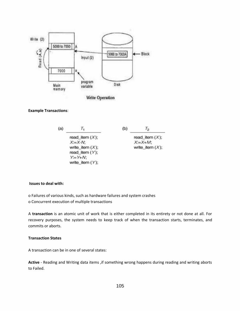
Example Transactions:
Issues to deal with:
o Failures of various kinds, such as hardware failures and system crashes
o Concurrent execution of multiple transactions
A transaction is an atomic unit of work that is either completed in its entirety or not done at all. For
recovery purposes, the system needs to keep track of when the transaction starts, terminates, and
commits or aborts.
Transaction States
A transaction can be in one of several states:
Active - Reading and Writing data items ,if something wrong happens during reading and writing aborts
to Failed.
105

Partially Committed - All reading and writing operations are done aborts to Failed when rollback occurs
or committed when commit occurs.
Committed - Transaction successfully completed and all write operations made permanent in the
Database
Failed - Transaction halted and all operations rolled back
Terminated - terminates either commits or failed
nt of database management systems
ACID Properties
106
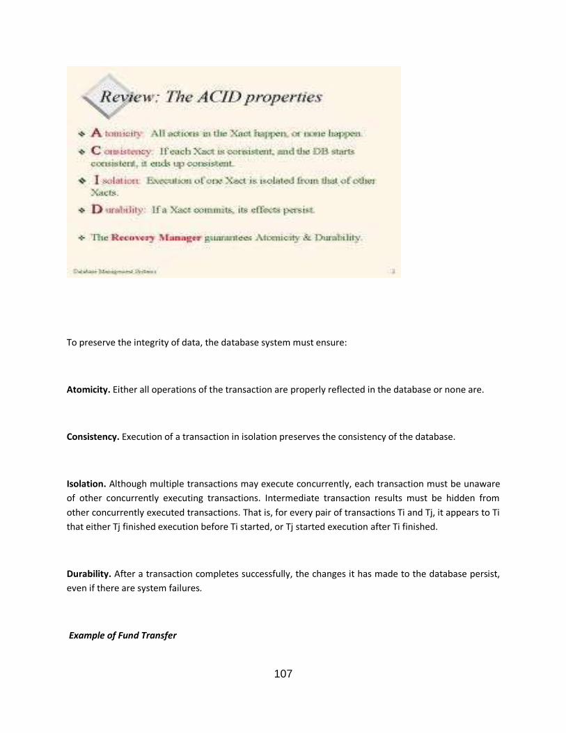
To preserve the integrity of data, the database system must ensure:
Atomicity. Either all operations of the transaction are properly reflected in the database or none are.
Consistency. Execution of a transaction in isolation preserves the consistency of the database.
Isolation. Although multiple transactions may execute concurrently, each transaction must be unaware
of other concurrently executing transactions. Intermediate transaction results must be hidden from
other concurrently executed transactions. That is, for every pair of transactions Ti and Tj, it appears to Ti
that either Tj finished execution before Ti started, or Tj started execution after Ti finished.
Durability. After a transaction completes successfully, the changes it has made to the database persist,
even if there are system failures.
Example of Fund Transfer
107

Transaction to transfer $50 from account A to account B:
1. read( A)
2. A:= A- 50
3. write( A)
4. read(B)
5. B:= B+ 50
6. write( B)
Atomicity requirement :
1. if the transaction fails after step 3 and before step 6, money will be “lost” leading to an inconsistent database state
2. The system should ensure that updates of a partially executed transaction are not reflected in the database
Durability requirement :
once the user has been notified that the transaction has completed (i.e., the transfer of the
$50 has taken place), the updates to the database by the transaction must persist even if there are
software or hardware failures.
Consistency requirement :
the sum of A and B is unchanged by the execution of the transaction
In general, consistency requirements include
Explicitly specified integrity constraints such as primary keys and foreign keys
108

Implicit integrity constraints
A transaction must see a consistent database.
During transaction execution the database may be temporarily inconsistent.
When the transaction completes successfully the database must be consistent
Erroneous transaction logic can lead to inconsistency
Isolation requirement :
if between steps 3 and 6, another transaction T2 is allowed to access the partially updated
database, it will see an inconsistent database (the sum A+B will be less than it should be). Isolation can
be ensured trivially by running transactions serially, that is, one after the other. However, executing
multiple transactions concurrently has significant benefits.
Transaction states:
Active state
Partially committed state
Committed state
Failed state
Terminated State
Recovery manager keeps track of the following operations:
o begin_transaction: This marks the beginning of transaction execution.
o read or write: These specify read or write operations on the database items that are executed as part of a transaction.
109

o end_transaction: This specifies that read and write transaction operations have ended and marks the end limit of transaction execution.
At this point it may be necessary to check whether the changes introduced by the transaction can be permanently applied to the database or whether the transaction has to be aborted because it violates concurrency control or for some other reason.
o commit_transaction: This signals a successful end of the transaction so that any changes (updates) executed by the transaction can be safely committed to the database and will not be undone.
o rollback (or abort): This signals that the transaction has ended unsuccessfully, so that any changes or effects that the transaction may have applied to the database must be undone.
Recovery techniques use the following operators:
o undo: Similar to rollback except that it applies to a single operation rather than to a whole transaction.
o redo: This specifies that certain transaction operations must be redone to ensure that all the operations of a committed transaction have been applied successfully to the database.
Two Main Techniques
Deferred Update
No physical updates to db until after a transaction commits.
During the commit, log records are made then changes are made permanent on disk.
What if a Transaction fails?
No UNDO required
REDO may be necessary if the changes have not yet been made permanent before the
failure.
110
Immediate Update
Physical updates to db may happen before a transaction commits.
All changes are written to the permanent log (on disk) before changes are made to the DB.
What if a Transaction fails?
After changes are made but before commit – need to UNDO the changes
REDO may be necessary if the changes have not yet been made permanent before the
failure
Recovery based on Deferred Update
Deferred update
Changes are made in memory and after T commits, the changes are made permanent on disk.
Changes are recorded in buffers and in log file during T’s execution.
At the commit point, the log is force-written to disk and updates are made in database.
No need to ever UNDO operations because changes are never made permanent
REDO is needed if the transaction fails after the commit but before the changes are made on disk.
Hence the name is NO UNDO/REDO algorithm
2 lists are maintained:
Commit list: committed transactions since last checkpoint
Active list: active transactions
REDO all write operations from commit list in order that they were written to the log
Active transactions are cancelled & must be resubmitted.
111

Recovery based on Immediate Update
Immediate update:
Updates to disk can happen at any time
But, updates must still first be recorded in the system logs (on disk) before changes are made to the
database.
Need to provide facilities to UNDO operations which have affected the db
2 flavors of this algorithm
UNDO/NO_REDO recovery algorithm
if the recovery technique ensures that all updates are made to the database on disk
before T commits, we do not need to REDO any committed transactions
UNDO/REDO recovery algorithm
Transaction is allowed to commit before all its changes are written to the database
o (Note that the log files would be complete at the commit point)
UNDO/REDO Algorithm
2 lists maintained:
Commit list: committed transactions since last checkpoint
Active list: active transactions
UNDO all write operations of active transactions.
Undone in the reverse of the order in which they were written to the log
REDO all write operations of the committed transactions
In the order in which they were written to the log.
Transaction:
112

Action, or series of actions, carried out by user or application, which accesses or changes
contents of database. It Transforms database from one consistent state to another, although
consistency may be violated during transaction
Logical unit of database processing that includes one or more access operations (read -retrieval,
write - insert or update, delete).
Transaction is an executing program forming a logical unit of database access operations that
involves one or more database operations (read -retrieval, write - insert or update, delete).
A transaction may be stand-alone set of operations specified in a high level language like SQL
submitted interactively, or may be embedded within a program.
A transaction must see a consistent database.
During transaction execution the database may be inconsistent.
When the transaction is committed, the database must be consistent.
Transaction boundaries:
Begin and End transaction.
An application program may contain several transactions separated by the Begin and End transaction
boundaries.
Two Basic operations are read and write
3) read_item(X): Reads a database item named X into a program variable. To simplify our notation, we assume that the program variable is also named X.
4) write_item(X): Writes the value of program variable X into the database item named X.
Why Do We Need Transactions?
It’s all about fast query response time and correctness
DBMS is a multi-user systems Many different requests Some against same data items
Figure out how to interleave requests to shorten response time while guaranteeing correct result
How does DBMS know which actions belong together?
Group database operations that must be performed together into transactions
Either execute all operations or none
READ AND WRITE OPERATIONS:
113

Basic unit of data transfer from the disk to the computer main memory is one block. In general,
a data item (what is read or written) will be the field of some record in the database, although it may be
a larger unit such as a record or even a whole block.
read_item(X) command includes the following steps:
4. Find the address of the disk block that contains item X. 5. Copy that disk block into a buffer in main memory (if that disk block is not already in
some main memory buffer). 6. Copy item X from the buffer to the program variable named X.
write_item(X) command includes the following steps:
5. Find the address of the disk block that contains item X. 6. Copy that disk block into a buffer in main memory (if that disk block is not already in some main
memory buffer). 7. Copy item X from the program variable named X into its correct location in the buffer. 8. Store the updated block from the buffer back to disk (either immediately or at some later point
in time).
114

Example Transactions:
Issues to deal with:
o Failures of various kinds, such as hardware failures and system crashes
o Concurrent execution of multiple transactions
A transaction is an atomic unit of work that is either completed in its entirety or not done at all. For
recovery purposes, the system needs to keep track of when the transaction starts, terminates, and
commits or aborts.
Transaction States
A transaction can be in one of several states:
Active - Reading and Writing data items ,if something wrong happens during reading and writing aborts
to Failed.
115

Partially Committed - All reading and writing operations are done aborts to Failed when rollback occurs
or committed when commit occurs.
Committed - Transaction successfully completed and all write operations made permanent in the
Database
Failed - Transaction halted and all operations rolled back
Terminated - terminates either commits or failed
nt of database management systems
ACID Properties
116

To preserve the integrity of data, the database system must ensure:
Atomicity. Either all operations of the transaction are properly reflected in the database or none are.
Consistency. Execution of a transaction in isolation preserves the consistency of the database.
Isolation. Although multiple transactions may execute concurrently, each transaction must be unaware
of other concurrently executing transactions. Intermediate transaction results must be hidden from
other concurrently executed transactions. That is, for every pair of transactions Ti and Tj, it appears to Ti
that either Tj finished execution before Ti started, or Tj started execution after Ti finished.
Durability. After a transaction completes successfully, the changes it has made to the database persist,
even if there are system failures.
Example of Fund Transfer
117
Transaction to transfer $50 from account A to account B:
1. read( A)
2. A:= A- 50
3. write( A)
4. read(B)
5. B:= B+ 50
6. write( B)
Atomicity requirement :
3. if the transaction fails after step 3 and before step 6, money will be “lost” leading to an inconsistent database state
4. The system should ensure that updates of a partially executed transaction are not reflected in the database
Durability requirement :
once the user has been notified that the transaction has completed (i.e., the transfer of the
$50 has taken place), the updates to the database by the transaction must persist even if there are
software or hardware failures.
Consistency requirement :
the sum of A and B is unchanged by the execution of the transaction
In general, consistency requirements include
Explicitly specified integrity constraints such as primary keys and foreign keys
118

Implicit integrity constraints
A transaction must see a consistent database.
During transaction execution the database may be temporarily inconsistent.
When the transaction completes successfully the database must be consistent
Erroneous transaction logic can lead to inconsistency
Isolation requirement :
if between steps 3 and 6, another transaction T2 is allowed to access the partially updated
database, it will see an inconsistent database (the sum A+B will be less than it should be). Isolation can
be ensured trivially by running transactions serially, that is, one after the other. However, executing
multiple transactions concurrently has significant benefits.
Transaction states:
Active state
Partially committed state
Committed state
Failed state
Terminated State
Recovery manager keeps track of the following operations:
o begin_transaction: This marks the beginning of transaction execution.
o read or write: These specify read or write operations on the database items that are executed as part of a transaction.
119

o end_transaction: This specifies that read and write transaction operations have ended and marks the end limit of transaction execution.
At this point it may be necessary to check whether the changes introduced by the transaction can be permanently applied to the database or whether the transaction has to be aborted because it violates concurrency control or for some other reason.
o commit_transaction: This signals a successful end of the transaction so that any changes (updates) executed by the transaction can be safely committed to the database and will not be undone.
o rollback (or abort): This signals that the transaction has ended unsuccessfully, so that any changes or effects that the transaction may have applied to the database must be undone.
Recovery techniques use the following operators:
o undo: Similar to rollback except that it applies to a single operation rather than to a whole transaction.
o redo: This specifies that certain transaction operations must be redone to ensure that all the operations of a committed transaction have been applied successfully to the database.
Two Main Techniques
Deferred Update
No physical updates to db until after a transaction commits.
During the commit, log records are made then changes are made permanent on disk.
What if a Transaction fails?
No UNDO required
REDO may be necessary if the changes have not yet been made permanent before the
failure.
120

Immediate Update
Physical updates to db may happen before a transaction commits.
All changes are written to the permanent log (on disk) before changes are made to the DB.
What if a Transaction fails?
After changes are made but before commit – need to UNDO the changes
REDO may be necessary if the changes have not yet been made permanent before the
failure
Recovery based on Deferred Update
Deferred update
Changes are made in memory and after T commits, the changes are made permanent on disk.
Changes are recorded in buffers and in log file during T’s execution.
At the commit point, the log is force-written to disk and updates are made in database.
No need to ever UNDO operations because changes are never made permanent
REDO is needed if the transaction fails after the commit but before the changes are made on disk.
Hence the name is NO UNDO/REDO algorithm
2 lists are maintained:
Commit list: committed transactions since last checkpoint
Active list: active transactions
REDO all write operations from commit list in order that they were written to the log
Active transactions are cancelled & must be resubmitted.
121
Recovery based on Immediate Update
Immediate update:
Updates to disk can happen at any time
But, updates must still first be recorded in the system logs (on disk) before changes are made to the
database.
Need to provide facilities to UNDO operations which have affected the db
2 flavors of this algorithm
UNDO/NO_REDO recovery algorithm
if the recovery technique ensures that all updates are made to the database on disk
before T commits, we do not need to REDO any committed transactions
UNDO/REDO recovery algorithm
Transaction is allowed to commit before all its changes are written to the database
o (Note that the log files would be complete at the commit point)
UNDO/REDO Algorithm
2 lists maintained:
Commit list: committed transactions since last checkpoint
Active list: active transactions
UNDO all write operations of active transactions.
Undone in the reverse of the order in which they were written to the log
REDO all write operations of the committed transactions
In the order in which they were written to the log.
122

Introduction to Concurrency
What is concurrency?
Concurrency in terms of databases means allowing multiple users to access the data
contained within a database at the same time. If concurrent access is not managed by the
Database Management System (DBMS) so that simultaneous operations don't interfere with one
another problems can occur when various transactions interleave, resulting in an inconsistent
database.
Concurrency is achieved by the DBMS, which interleaves actions (reads/writes of DB objects)
of various transactions. Each transaction must leave the database in a consistent state if the DB is
consistent when the transaction begins. Concurrent execution of user programs is essential for
good DBMS performance. Because disk accesses are frequent, and relatively slow, it is
important to keep the CPU humming by working on several user programs concurrently.
Interleaving actions of different user programs can lead to inconsistency: e.g., check is cleared
while account balance is being computed. DBMS ensures such problems don’t arise: users can
pretend they are using a single-user system.
Purpose of Concurrency Control
o To enforce Isolation (through mutual exclusion) among conflicting transactions.
o To preserve database consistency through consistency preserving execution of
transactions.
o To resolve read-write and write-write conflicts.
Example: In concurrent execution environment if T1 conflicts with T2 over a data item A, then
the existing concurrency control decides if T1 or T2 should get the A and if the other transaction
is rolled-back or waits.
Timestamp based concurrency control algorithm
Timestamp
123
A monotonically increasing variable (integer) indicating the age of an
operation or a transaction. A larger timestamp value indicates a more
recent event or operation.
Timestamp based algorithm uses timestamp to serialize the execution of
concurrent transactions.
Basic Timestamp Ordering
1. Transaction T issues a write_item(X) operation:
If read_TS(X) > TS(T) or if write_TS(X) > TS(T), then an younger
transaction has already read the data item so abort and roll-back T and
reject the operation.
If the condition in part (a) does not exist, then execute write_item(X) of T
and set write_TS(X) to TS(T).
2. Transaction T issues a read_item(X) operation:
If write_TS(X) > TS(T), then an younger transaction has already written to
the data item so abort and roll-back T and reject the operation.
If write_TS(X) TS(T), then execute read_item(X) of T and set
read_TS(X) to the larger of TS(T) and the current read_TS(X).
Strict Timestamp Ordering
1. Transaction T issues a write_item(X) operation:
If TS(T) > read_TS(X), then delay T until the transaction T’ that wrote or
read X has terminated (committed or aborted).
2. Transaction T issues a read_item(X) operation:
If TS(T) > write_TS(X), then delay T until the transaction T’ that wrote or
read X has terminated (committed or aborted).
Multiversion concurrency control techniques
o This approach maintains a number of versions of a data item and allocates the
right version to a read operation of a transaction. Thus unlike other mechanisms a
read operation in this mechanism is never rejected.
o Side effect:
Significantly more storage (RAM and disk) is required to maintain
multiple versions. To check unlimited growth of versions, a garbage
collection is run when some criteria is satisfied.
124

o This approach maintains a number of versions of a data item and allocates the
right version to a read operation of a transaction.
Thus unlike other mechanisms a read operation in this mechanism is never
rejected.
Multiversion technique based on timestamp ordering
Assume X1, X2, …, Xn are the version of a data item X created by a write operation of
transactions. With each Xi a read_TS (read timestamp) and a write_TS (write
timestamp) are associated.
read_TS(Xi): The read timestamp of Xi is the largest of all the timestamps of
transactions that have successfully read version Xi.
write_TS(Xi): The write timestamp of Xi that wrote the value of version Xi.
A new version of Xi is created only by a write operation.
To ensure serializability, the following two rules are used.
1. . If transaction T issues write_item (X) and version i of X has the highest
write_TS(Xi) of all versions of X that is also less than or equal to TS(T), and read
_TS(Xi) > TS(T), then abort and roll-back T; otherwise create a new version Xi and
read_TS(X) = write_TS(Xj) = TS(T).
2. If transaction T issues read_item (X), find the version i of X that has the highest
write_TS(Xi) of all versions of X that is also less than or equal to TS(T), then return the
value of Xi to T, and set the value of read _TS(Xi) to the largest of TS(T) and the current
read_TS(Xi).
Rule 2 guarantees that a read will never be rejected.
Multiversion Two-Phase Locking Using Certify Locks
Concept
o Allow a transaction T’ to read a data item X while it is write locked by a
conflicting transaction T.
125

o This is accomplished by maintaining two versions of each data item X where one
version must always have been written by some committed transaction. This
means a write operation always creates a new version of X. Multiversion Two-Phase Locking Using Certify Locks
Steps
1. X is the committed version of a data item.
2. T creates a second version X’ after obtaining a write lock on X.
3. Other transactions continue to read X.
4. T is ready to commit so it obtains a certify lock on X’.
5. The committed version X becomes X’.
6. T releases its certify lock on X’, which is X now.
Compatibility tables for basic 2pl and 2pl with certify locks:-
Note:
In multiversion 2PL read and write operations from conflicting transactions can be
processed concurrently.
This improves concurrency but it may delay transaction commit because of obtaining
certify locks on all its writes. It avoids cascading abort but like strict two phase locking
scheme conflicting transactions may get deadlocked.
Validation (Optimistic) Concurrency Control Schemes
Read Write
yes no
no no
Read
Write
Read Write Certify
yes no no
no no no
no no no
Read
Write
Certify
126

In this technique only at the time of commit serializability is checked and transactions
are aborted in case of non-serializable schedules.
Three phases:
1. Read phase
2. Validation phase
3. Write phase 1. Read phase:
A transaction can read values of committed data items. However, updates are applied
only to local copies (versions) of the data items (in database cache).
2.Validation phase: Serializability is checked before transactions write their updates to the
database.
o This phase for Ti checks that, for each transaction Tj that is either committed or is
in its validation phase, one of the following conditions holds:
Tj completes its write phase before Ti starts its read phase.
Ti starts its write phase after Tj completes its write phase, and the read_set
of Ti has no items in common with the write_set of Tj
Both the read_set and write_set of Ti have no items in common with the
write_set of Tj, and Tj completes its read phase.
When validating Ti, the first condition is checked first for each transaction
Tj, since (1) is the simplest condition to check. If (1) is false then (2) is
checked and if (2) is false then (3 ) is checked. If none of these conditions
holds, the validation fails and Ti is aborted.
3.Write phase: On a successful validation transactions’ updates are applied to the database;
otherwise, transactions are restarted.
LOCK
Definition : Lock is a variable associated with data item which gives the status whether the
possible operations can be applied on it or not.
Two-Phase Locking Techniques:
Binary locks: Locked/unlocked
The simplest kind of lock is a binary on/off lock. This can be
created by storing a lock bit with each database item. If the lock bit is on (e.g. = 1) then the item
127
cannot be accessed by any transaction either for reading or writing, if it is off (e.g. = 0) then the
item is available. Enforces mutual exclusion
Binary locks are:
Simple but are restrictive.
Transactions must lock every data item that is read or written
No data item can be accessed concurrently
Locking is an operation which secures
(a) permission to Read
(b) permission to Write a data item for a transaction.
Example: Lock (X). Data item X is locked in behalf of the requesting transaction.
Unlocking is an operation which removes these permissions from the data item.
Example:Unlock (X): Data item X is made available to all other transactions.
• Lock and Unlock are Atomic operations.
• Lock Manager: Managing locks on data items.
• Lock table:
• Lock manager uses it to store the identify of transaction locking a data item, the data
item, lock mode . One simple way to implement a lock table is through linked list.
< locking_transaction ,data item, LOCK >
The following code performs the lock operation:
B: if LOCK (X) = 0 (*item is unlocked*)
then LOCK (X) 1 (*lock the item*)
else begin
wait (until lock (X) = 0) and
the lock manager wakes up the transaction);
128

goto B
end;
The following code performs the unlock operation:
LOCK (X) 0 (*unlock the item*)
if any transactions are waiting then
wake up one of the waiting the transactions;
Multiple-mode locks: Read/write
– a.k.a. Shared/Exclusive
• Three operations
– read_lock(X)
– write_lock(X)
– unlock(X)
• Each data item can be in one of three lock states
– Three locks modes:
• (a) shared (read) (b) exclusive (write) (c) unlock(release)
– Shared mode: shared lock (X)
More than one transaction can apply share lock on X for reading its value
but no write lock can be applied on X by any other transaction.
– Exclusive mode: Write lock (X)
Only one write lock on X can exist at any time and no shared lock can be
applied by any other transaction on X.
_ Unlock mode: Unlock(X)
After reading or writing the corresponding transaction releases by
issuing this.
The rules for multiple-mode locking schemes are a transaction T:
Issue a read_lock(X) or a write_lock(X) before read(X)
Issue a write_lock(X) before write(X)
Issue an unlock(X) after all read(X) and write(X) are finished
129

The transaction T
Will not issue read_lock (X) or write_lock(X) if it already holds a lock on X
Will not issue unlock(X) unless it already holds a lock on X
Lock table:
Lock manager uses it to store the identify of transaction locking a data item,
the data item, lock mode and no of transactions that are currently reading the
data item . It looks like as below
<data item,read_ LOCK,nooftransactions,transaction id >
This protocol isn’t enough to guarantee serializability. If locks are released too early, you can
create problems. This usually happens when a lock is released before another lock is acquired.
The following code performs the read operation:
B: if LOCK (X) = “unlocked” then
begin LOCK (X) “read-locked”;
no_of_reads (X) 1;
end
else if LOCK (X) “read-locked” then
no_of_reads (X) no_of_reads (X) +1
else begin wait (until LOCK (X) = “unlocked” and
the lock manager wakes up the transaction);
go to B
end;
130

The following code performs the write lock operation:
B: if LOCK (X) = “unlocked” then
LOCK (X) “write-locked”;
else begin wait (until LOCK (X) = “unlocked” and
the lock manager wakes up the transaction);
go to B
end;
The following code performs the unlock operation:
if LOCK (X) = “write-locked” then
begin LOCK (X) “unlocked”;
wakes up one of the transactions, if any
end
else if LOCK (X) “read-locked” then
begin
no_of_reads (X) no_of_reads (X) -1
if no_of_reads (X) = 0 then
begin
LOCK (X) = “unlocked”;
wake up one of the transactions, if any
end
end;
Lock conversion:
131

Lock upgrade: existing read lock to write lock
if Ti has a read-lock (X) and Tj has no read-lock (X) (i j) then convert read-lock (X) to
write-lock (X)
else
force Ti to wait until Tj unlocks X
Lock downgrade: existing write lock to read lock
Ti has a write-lock (X) (*no transaction can have any lock on X*)
convert write-lock (X) to read-lock (X)
Two-Phase Locking Techniques: The algorithm
The timing of locks is also important in avoiding concurrency problems. A simple requirement to
ensure transactions are serializable is that all read and write locks in a transaction are issued
before the first unlock operation known as a two-phase locking protocol.
Transaction divided into 2 phases:
growing - new locks acquired but none released
shrinking - existing locks released but no new ones acquired
During the shrinking phase no new locks can be acquired!
– Downgrading ok
– Upgrading is not
Rules of 2PL are as follows:
If T wants to read an object it needs a read_lock
If T wants to write an object, it needs a write_lock
Once a lock is released, no new ones can be acquired.
The 2PL protocol guarantees serializability
Any schedule of transactions that follow 2PL will be serializable
132

We therefore do not need to test a schedule for serializability
But, it may limit the amount of concurrency since transactions may have to hold onto locks
longer than needed, creating the new problem of deadlocks.
Two-Phase Locking Techniques: The algorithm
Here is a example without 2PL:-
T1 T2 Result
read_lock (Y); read_lock (X); Initial values: X=20; Y=30
read_item (Y); read_item (X); Result of serial execution
unlock (Y); unlock (X); T1 followed by T2
write_lock (X); Write_lock (Y); X=50, Y=80.
read_item (X); read_item (Y); Result of serial execution
X:=X+Y; Y:=X+Y; T2 followed by T1
write_item (X); write_item (Y); X=70, Y=50
unlock (X); unlock (Y);
T1 T2 Result
read_lock (Y); X=50; Y=50
read_item (Y); Nonserializable because it.
unlock (Y); violated two-phase policy.
read_lock (X);
read_item (X);
unlock (X);
write_lock (Y);
read_item (Y);
133

Y:=X+Y;
write_item (Y);
unlock (Y);
write_lock (X);
read_item (X);
X:=X+Y;
write_item (X);
unlock (X);
Here is a example with 2PL:-
T’1 T’2 Result
read_lock (Y); read_lock (X); T1 and T2 follow two-phase
read_item (Y); read_item (X); policy but they are subject to
write_lock (X); Write_lock (Y); deadlock, which must be
unlock (Y); unlock (X); dealt with.
read_item (X); read_item (Y);
X:=X+Y; Y:=X+Y;
write_item (X); write_item (Y);
unlock (X); unlock (Y);
Two-phase policy generates four locking algorithms:-
1. BASIC
2. CONSERVATIVE
3. STRICT
4. RIGOUROUS
134

• Previous technique knows as basic 2PL
• Conservative 2PL (static) 2PL: Lock all items needed BEFORE execution begins by
predeclaring its read and write set
– If any of the items in read or write set is already locked (by other transactions),
transaction waits (does not acquire any locks)
– Deadlock free but not very realistic
• Strict 2PL: Transaction does not release its write locks until AFTER it aborts/commits
– Not deadlock free but guarantees recoverable schedules (strict schedule:
transaction can neither read/write X until last transaction that wrote X has
committed/aborted)
– Most popular variation of 2PL
• Rigorous 2PL: No lock is released until after abort/commit
Transaction is in its expanding phase until it ends
The Two-Phase Locking Protocol
Introduction
This is a protocol, which ensures conflict-serializable schedules.
Phase 1: Growing Phase
– Transaction may obtain locks.
– Transaction may not release locks.
Phase 2: Shrinking Phase
– Transaction may release locks.
– Transaction may not obtain locks.
– The protocol assures serializability. It can be proved that the transactions
can be serialized in the order of their lock points.
– Lock points: It is the point where a transaction acquired its final lock.
– Two-phase locking does not ensure freedom from deadlocks
– Cascading rollback is possible under two-phase locking.
– There can be conflict serializable schedules that cannot be obtained if
two-phase locking is used.
Given a transaction Ti that does not follow two-phase locking, we can find a
transaction Tj that uses two-phase locking, and a schedule for Ti and Tj that is not
135
conflict serializable.
Lock Conversions
Two-phase locking with lock conversions:
First Phase:
_ can acquire a lock-S on item
_ can acquire a lock-X on item
_ can convert a lock-S to a lock-X (upgrade)
Second Phase:
_ can release a lock-S
_ can release a lock-X
_ can convert a lock-X to a lock-S (downgrade)
This protocol assures serializability. But still relies on the programmer to insert
the various locking instructions.
Automatic Acquisition of Locks
A transaction Ti issues the standard read/write instruction, without explicit locking calls.
The operation read( D) is processed as:
if Ti has a lock on D
then
read( D)
else
begin
if necessary wait until no other
transaction has a lock-X on D
grant Ti a lock-S on D;
read( D)
136

end;
write( D) is processed as:
if Ti has a lock-X on D
then
write( D)
else
begin
if necessary wait until no other trans. has any lock on D,
if Ti has a lock-S on D
then
upgrade lock on Dto lock-X
else
grant Ti a lock-X on D
write( D)
end;All locks are released after commit or abort
Graph-Based Protocols
It is an alternative to two-phase locking.
Impose a partial ordering on the set D = f d1, d2 , ..., dhg of all data items.
If di! dj, then any transaction accessing both di and dj must access di before accessing dj.
Implies that the set D may now be viewed as a directed acyclic graph, called a database
graph.
Tree-protocol is a simple kind of graph protocol.
Tree Protocol
Only exclusive locks are allowed.
137

The first lock by Ti may be on any data item. Subsequently, Ti can lock a data item Q,
only if Ti currently locks the parent of Q.
Data items may be unlocked at any time.
A data item that has been locked and unlocked by Ti cannot subsequently be re-locked
by Ti.
The tree protocol ensures conflict serializability as well as freedom from deadlock.
Unlocking may occur earlier in the tree-locking protocol than in the twophase locking
protocol.
However, in the tree-locking protocol, a transaction may have to lock data items that it
does not access.
Increased locking overhead, and additional waiting time. Schedules not possible under
two-phase locking are possible under tree
protocol, and vice versa.
Granularity of data items and Multiple Granularity Locking
A lockable unit of data defines its granularity. Granularity can be coarse (entire
database) or it can be fine (a tuple or an attribute of a relation).
Data item granularity significantly affects concurrency control performance. Thus,
the degree of concurrency is low for coarse granularity and high for fine granularity.
Example of data item granularity:
1. A field of a database record (an attribute of a tuple)
2. A database record (a tuple or a relation)
3. A disk block
4. An entire file
5. The entire database
The following diagram illustrates a hierarchy of granularity from coarse (database) to fine
(record).
To manage such hierarchy, in addition to read and write, three additional locking modes,
called intention lock modes are defined:
o Intention-shared (IS): indicates that a shared lock(s) will be requested on some
descendent nodes(s).
o Intention-exclusive (IX): indicates that an exclusive lock(s) will be requested on
some descendent node(s).
DB
f1 f2
p11 p12 ... p1n
r111 ... r11j r111 ... r11j r111 ... r11j r111 ... r11j r111 ... r11j r111 ... r11j
p11 p12 ... p1n
138

o Shared-intention-exclusive (SIX): indicates that the current node is locked in
shared mode but an exclusive lock(s) will be requested on some descendent
nodes(s).
These locks are applied using the following compatibility matrix:
The set of rules which must be followed for producing serializable schedule are
1. The lock compatibility must adhered to.
2. The root of the tree must be locked first, in any mode..
3. A node N can be locked by a transaction T in S or IX mode only if the parent
node is already locked by T in either IS or IX mode.
4. A node N can be locked by T in X, IX, or SIX mode only if the parent of N is
already locked by T in either IX or SIX mode.
5. T can lock a node only if it has not unlocked any node (to enforce 2PL policy).
6. T can unlock a node, N, only if none of the children of N are currently locked by
T.
Granularity of data items and Multiple Granularity Locking: An example of a serializable
execution:
T1 T2 T3
IX(db)
IX(f1)
IX(db)
IS(db)
IS IX S SIX X
yes yes yes yes no
yes yes no no no
yes no yes no no
yes no no no no
no no no no no
IS
IX
S
SIX
X
139
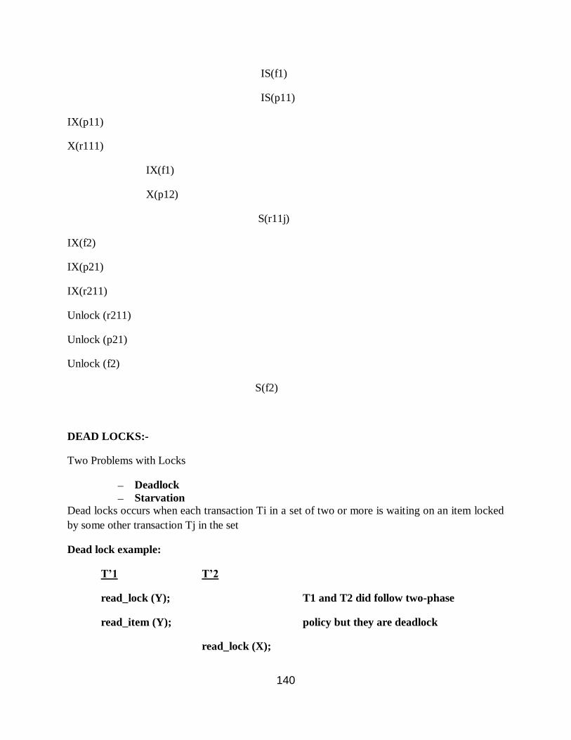
IS(f1)
IS(p11)
IX(p11)
X(r111)
IX(f1)
X(p12)
S(r11j)
IX(f2)
IX(p21)
IX(r211)
Unlock (r211)
Unlock (p21)
Unlock (f2)
S(f2)
DEAD LOCKS:-
Two Problems with Locks
– Deadlock
– Starvation
Dead locks occurs when each transaction Ti in a set of two or more is waiting on an item locked
by some other transaction Tj in the set
Dead lock example:
T’1 T’2
read_lock (Y); T1 and T2 did follow two-phase
read_item (Y); policy but they are deadlock
read_lock (X);
140

read_item (X);
write_lock (X);
(waits for X) write_lock (Y);
(waits for Y)
Deadlock Prevention
• Locking as deadlock prevention leads to very inefficient schedules (e.g., conservative
2PL)
• Better, use transaction timestamp TS(T)
– TS is unique identifier assigned to each transaction
– if T1 starts before T2, then TS(T1) < TS(T2) (older has smaller timestamp value)
– Wait-die and wound-wait schemes
Wait-Die Scheme
• Assume Ti tries to lock X which is locked by Tj
• If TS(Ti) < TS(Tj) (Ti older than Tj), then Ti is allowed to wait
• Otherwise, Ti younger than Tj, abort Ti (Ti dies) and restart later with SAME timestamp
• Older transaction is allowed to wait on younger transaction
• Younger transaction requesting an item held by older transaction is aborted and restarted
Wound-Wait Scheme
• Assume Ti tries to lock X which is locked by Tj
• If TS(Ti) < TS(Tj) (Ti older than Tj), abort Tj (Ti wounds Tj) and restart later with
SAME timestamp
• Otherwise, Ti younger than Tj, Ti is allowed to wait
• Younger transaction is allowed to wait on older transaction
• Older transaction requesting item held by younger transaction preempts younger one by
aborting it
• Both schemes abort younger transaction that may be involved in deadlock
• Both deadlock free but may cause needless aborts
141

More Deadlock Prevention
• Waiting schemes (require no timestamps)
• No waiting: if transaction cannot obtain lock, aborted immediately and restarted after
time t needless restarts
• Cautious waiting:
– Suppose Ti tries to lock item X which is locked by Tj
– If Tj is not blocked, Ti is blocked and allowed to wait
– O.w. abort Ti
– Cautious waiting is deadlock-free
Deadlock Detection
• DBMS checks if deadlock has occurred
– Works well if few short transactions with little interference
– O.w., use deadlock prevention
• Two approaches to deadlock detection:
1. Wait-for graph
– If cycle, abort one of the transactions (victim selection)
2. Timeouts
Starvation
• Transaction cannot continue for indefinite amount of time while others proceed normally
• When? Unfair waiting scheme with priorities for certain transactions E.g., in deadlock
detection, if we choose victim always based on cost factors, same transaction may always
be picked as victim
– Include rollbacks in cost factor
142

UNIT IV
TRENDS IN DATABASE TECHNOLOGY
Classification o f Physical Storage Media
Based on Speed with which data can be accessed Based on Cost per unit of data Based on
eliability Data loss on power failure or system crash Physical failure of the storage device H
Based on life of storage Volatile storage: loses contents when power is switched off 4 Non-
volatile storage:
Contents persist even when power is switched off. Includes secondary and tertiary storage,
as well as batterbacked up main-memory.
Physical Storage Media Cache
The fastest and most costly form of storage Volatile Managed by the computer system hardware.
Main memory
4 Fast access (10s to 100s of nanoseconds; 1 nanosecond = 10–9 seconds) 4 Generally too small
(or too expensive) to store the entire database
Capacities of up to a few Gigabytes widely used currently Capacities have gone up and per-
byte costs have decreased steadily and rapidly
Volatile — contents of main memory are usually lost if a power failure or system crash occurs.
Flash memory
Data survives power failureData can be written at a location only once, but location can be
erased and written to again Can support only a limited number of write/erase cycles.
Erasing of memory has to be done to an entire bank of memory.
Reads are roughly as fast as main memory But writes are slow (few microseconds), erase is
slower Cost per unit of storage roughly similar to main memory Widely used in embedded
devices such as digital cameras Also known as EEPROM
Magnetic-disk
Data is stored on spinning disk,and read/written magneticallyPrimary medium for the long-term
storage of data;typically stores entire database.Data must be moved from disk to main memory
foraccess, and written back for storage
Much slower accessthan main memory (more on this later)
Direct-access – possible to read data on disk in any order,unlike magnetic tapeHard disks vs.
floppy disks Capacities range up to roughly 100 GB currently
Much larger capacity and cost/byte than main memory/ flash memory Growing constantly
and rapidly with technology improvements
Survives power failures and system crashes
Disk failure candestroy data, but is very rare.
Optical storage
Non-volatile, data is read optically from a spinning disk using a laser CD-ROM (640 MB) and
DVD (4.7 to 17 GB) most popular forms Write-one, read-many (WORM) optical disks used for
archival storage (CD-R and DVD-R) Multiple write versions also available (CD-RW, DVDRW,
143
and DVD-RAM) 4 Reads and writes are slower than with magnetic disk Juke-box systems, with
large numbers of removable disks, a few drives, and a mechanism for automatic
loading/unloading of disks available for storing large volumes of data.
Optical Disks
Compact disk-read only memory (CD-ROM) Disks can be loaded into or removed from a drive 4
High storage capacity (640 MB per disk) High seek times or about 100 msec (optical read head
is heavier and slower) Higher latency (3000 RPM) and lower data-transfer rates (3-6 MB/s)
compared to magnetic disks
Digital Video Disk (DVD)
DVD-5 holds 4.7 GB, and DVD-9 holds 8.5 GB DVD-10 and DVD-18 are double sided formats
with capacities of 9.4 GB & 17 GB Other characteristics similar to CD-ROM 4 Record once
versions (CD-R and DVD-R) Data can only be written once, and cannot be erased. High capacity
and long lifetime; used for archival storage 4Multi-write versions (CD-RW, DVD-RW and
DVDRAM) also available
Tape storage
Non-volatile, used primarily for backup (to recover from disk failure), and for archival data
Sequential-access – much slower than disk Very high capacity (40 to 300 GB tapes available)
Tape can be removed from drive storage costs much cheaper than disk, but drives are expensive
4 Tape jukeboxes available for storing massive amounts of data Hundreds of terabytes (1
terabyte = 109 bytes) to even apetabyte (1 petabyte = 1012 bytes)
Storage Hierarchy
Primary storage: Fastest media but volatile (cache, main memory).
Secondary storage: next level in hierarchy, non-volatile, moderately fast access time. Also
called on-line storage
4E.g. flash memory, magnetic disks
Tertiary storage: lowest level in hierarchy, non-volatile, slow access time Also called off-line
storage
E.g. magnetic tape, optical storage
Magnetic Hard Disk Mechanism
n Read-write head Positioned very close to the platter surface (almost touching it) Reads or
writes magnetically encoded information. Surface of platter divided into circular tracks Over
17,000 tracks per platter on typical hard disks Each track is divided into sectors. A sector is the
smallest unit of data that can be read or written. H Sector size typically 512 bytes Typical sectors
per track: 200 (on inner tracks) to 400 (on outer tracks) To read/write a sector Disk arm swings
to position head on right track Platter spins continually; data is read/written as sector passes
144
under head Head-disk assemblies Multiple disk platters on a single spindle (typically 2 to 4) One
head per platter, mounted on a common arm. Cylinder i consists of ith track of all the platters
Performance Measures of Disks
Access Time – the time it takes from when a read or write request is issued to when data
transfer begins. Consists of:
Seek Time – time it takes to reposition the arm over the correct track.
Average Seek Time is 1/2 the worst case seek time.
– Would be 1/3 if all tracks had the same number of sectors, and we ignore the time to start
and stop arm movement 4 to 10 milliseconds on typical disks
Rotational latency – time it takes for the sector to be accessed to appear under the head.
Average latency is 1/2 of the worst-case latency. 4 to 11 milliseconds on typical disks (5400
to 15000 r.p.m.) n Data-Transfer Rate – the rate at which data can be retrieved from or stored
to the disk. H4 to 8 MB per second is typical
Multiple disks may share a controller, so rate that controller can handle is also important
Mean Time To Failure (MTTF) – the average time the disk is expected to run continuously
without any failure. Typically 3 to 5 years Probability of failure of new disks is quite low,
corresponding to a ―theoretical MTTF‖ of 30,000 to 1,200,000 hours for a new disk.
RAID
RAID: Redundant Arrays of Independent Disks
disk organization techniques that manage a large numbers of disks, providing a view of a single
disk of high reliability by storing data redundantly, so that data can be recovered even if a disk
fails. The chance that some disk out of a set of N disks will fail is much higher than the chance
that a specific single disk will fail.
E.g., a system with 100 disks, each with MTTF of 100,000 hours (approx. 11 years), will have a
system MTTF of 1000 hours (approx. 41 days)
o Techniques for using redundancy to avoid data loss are critical with large numbers of disks
Originally a cost-effective alternative to large, expensive disks.
o I in RAID originally stood for ―inexpensive‘‘
o Today RAIDs are used for their higher reliability and bandwidth.
The ―I‖ is interpreted as independent
Improvement of Reliability via Redundancy
Redundancy – store extra information that can be used to rebuild information lost in a disk
failure.
E.g., Mirroring (or shadowing)
o Duplicate every disk. Logical disk consists of two physical disks.
o Every write is carried out on both disks
Reads can take place from either disk
o If one disk in a pair fails, data still available in the other
Data loss would occur only if a disk fails, and its mirror disk also fails before the system is
repaired.
Prob ability of combined event is very small o Except for dependent failure modes
145

such as fire or building collapse or electrical power surges.
Mean time to data loss depends on mean time to failure, and mean time to repair.
o E.g. MTTF of 100,000 hours, mean time to repair of 10 hours
gives mean time to data loss of 500*106 hours (or 57,000 years)
for a mirrored pair of disks (ignoring dependent failure modes)
Improvement in Performance via Parallelism
o Two main goals of parallelism in a disk system:
1. Load balance multiple small accesses to increase throughput
2. Parallelize large accesses to reduce response time.
o Improve transfer rate by striping data across multiple disks.
o Bit-level striping – split the bits of each byte across multiple disks
In an array of eight disks, write bit i of each byte to disk i.
Each access can read data at eight times the rate of a single disk.
But seek/access time worse than for a single disk
Bit level striping is not used much any more
o Block-level striping – with n disks, block i of a file goes to disk (i mod n) + 1
Requests for different blocks can run in parallel if the blocks reside on different disks.
A request for a long sequence of blocks can utilize all disks in parallel.
RAID Levels
o Schemes to provide redundancy at lower cost by using disk striping combined with parity bits.
Different RAID organizations, or RAID levels, have differing cost, performance and reliability
RAID Level 0: Block striping; non-redundant.
o Used in high-performance applications where data lost is not critical.
RAID Level 1: Mirrored disks with block striping.
o Offers best write performance.
o Popular for applications such as storing log files in a database system.
RAID Level 2: Memory-Style Error-Correcting-Codes (ECC) with bit striping.
RAID Level 5: Block-Interleaved Distributed Parity; partitions data and
parityNOTESamong all N + 1 disks, rather than storing data in N disks and parity in 1 disk.
o E.g., with 5 disks, parity block for nth set of blocks is stored on disk (n mod 5) + 1, with the
data
blocks stored on the other 4 disks. o Higher I/O rates than Level 4. Block writes occur in parallel
if the blocks and their parity blocks are on different disks. o Subsumes Level 4: provides same
benefits, but avoids bottleneck of parity disk. RAID Level 6: P+Q Redundancy scheme;
similar to Level 5, but stores extra redundant information to guard against multiple disk failures.
o Better reliability than Level 5 at a higher cost; not used as widely.
FILE OPERATIONS
The database is stored as a collection of files. Each file is a sequence of records. A record is a
sequence of fields.
One approach:
o assume record size is fixed.
o each file has records of one particular type only.
o different files are used for different relations.
This case is easiest to implement; will consider variable length records later.
146

Fixed-Length Records
Simple approach:
o Store record i starting from byte n (i – 1), where n is the size of each
record.
o Record access is simple but records may cross blocks
Modification: do not allow records to cross block boundaries.
Free List s
o Store the address of the first deleted record in the file header.
o Use this first record to store the address of the second deleted record, and so on.
o Can think of these stored addresses as pointers since they ―point‖ to the location of a
record.
o More space efficient representation: reuse space for normal attributes of free records to
store pointers. (No pointers stored in in-use records.)
Variable-Length Records
o Variable-length records arise in database systems in several ways:
Storage of multiple record types in a file.
Record types that allow variable lengths for one or more
fields.
Record types that allow repeating fields (used in some
older data models).
o Byte string representation
Attach an end-of-record ( ) control character to the end of each record.
Difficulty with deletion.
Difficulty with growth.
Variable-Length Records: Slotted Page Structure
Slotted page header contains: o number of record entries. o end of free space in the block. o
location and size of each record.
Records can be moved around within a page to keep them contiguous with no empty space
between them; entry in the header must be up-dated.
Pointers should not point directly to record — instead they should point to the entry for the
record in header.
Fixed-length representation:
o reserved space
o pointers
Reserved space – can use fixed-length records of a known maximum length; unused space in
shorter records filled with a null or end-of-record symbol.
Pointer Method
Pointer method
A variable-length record is represented by a list of fixed-length records, chained together via
pointers.
Can be used even if the maximum record length is not known
Disadvantage to pointer structure; space is wasted in all records except the first in a a chain.
Solution is to allow two kinds of block in file:
Anchor block – contains the first records of chain
Overflow block – contains records other than those that are the first records of chairs.
147

Organization of Records in Files
Heap – a record can be placed anywhere in the file where there is space
Sequential – store records in sequential order, based on the value of the search key of each
record
Hashing – a hash function computed on some attribute of each record; the result specifies in
which block of the file the record should be placed
Records of each relation may be stored in a separate file. In a clustering NOTES
file organization records of several different relations can be stored in
the same file
Motivation: store related records on the same block to minimize I/O
Sequential File Organization
Suitable for applications that require sequential processing of the entire file
The records in the file are ordered by a search-key
Deletion – use pointer chains
Insertion –locate the position where the record is to be inserted
if there is free space insert there
if no free space, insert the record in an overflow block
In either case, pointer chain must be updated
Need to reorganize the file from time to time to restore sequential order
Clustering File Organization
o Simple file structure stores each relation in a separate file.
o Can instead store several relations in one file using a clustering file organization.
o E.g., clustering organization of customer and depositor:
Mapping of Objects to Files
Mapping objects to files is similar to mapping tuples to files in a relational system; object data
can be stored using file structures.
Objects in O-O databases may lack uniformity and may be very large; such objects have to
managed differently from records in a relational system.
o Set fields with a small number of elements may be implemented using data structures such as
linked lists.
o Set fields with a larger number of elements may be implemented as separate relations in the
database.
o Se t fields can also be eliminated at the storage level by normalization.
Similar to conversion of multivalued attributes of E-R diagrams to relations
Objects are identified by an object identifier (OID); the storage system needs a mechanism to
locate an object given its OID (this action is called dereferencing).
o logical identifiers do not directly specify an object‘s physical location; must maintain an index
that
maps an OID to the object‘s actual location.
o physical identifiers encode the location of the object so the object can be found directly.
Physical
OIDs typically have the following parts:
1. a volume or file identifier
2. a page identifier within the volume or file
3. an offset within the page
148

HASHING
Hashing is a hash function computed on some attribute of each record; the result specifies in
which block of the file the record should be placed.
Static Hashing
A bucket is a unit of storage containing one or more records (a bucket is typically a disk block).
Hash function h is a function from the set of all search-key values K to the set of all bucket
addresses B.
Hash function is used to locate records for access, insertion as well as deletion.
Records with different search-key values may be mapped to the same bucket; thus entire bucket
has to be searched sequentially to locate a record.
Example of Hash File Organization
Hash file organization ofaccountfile, usingbranch-nameas keyo There are 10 buckets ,
o The binary representation of the ith character is assumed to be the integer i.
o The hash function returns the sum of the binary representations of the characters modulo 10.
o E.g. h(Perryridge) = 5 h(Round Hill) = 3 h(Brighton) = 3
o Hash file organization of account file, using branch-name as key
Hash Functions o Worst had function maps all search-key values to the same bucket; this makes access time
proportional to t he number of search-key values in the file.
o An ideal hash function is uniform, i.e., each bucket is assigned the same number of search-key
values from the set of all possible values.
o Ideal hash function is random, so each bucket will have the same number of records assigned
to
it irrespective of the actual distribution of search-key values in the file.
o Typical hash functions perform computation on the internal binary representation of the
searchkey.
o For example, for a string search-key, the binary representations of all the characters in the
string
could be added and the sum modulo the number of buckets could be returned.
Handling of Bucket Overflows
o Bucket overflow can occur because of
Insufficient buckets
Skew in distribution of r ecords. This can occur due to two reasons:
multiple records have same search-key value
chosen hash function produces non-uniform distribution of key values
o Although the probability of bucket overflow can be reduced, it cannot be eliminated; it is
handled
by using overflow buckets.
o Overflow chaining – the overflow buckets of a given bucket are chained together in a linked
list.
o The Above scheme is called closed hashing.
o An alternative, called open hashing, which does not use overflow buckets, is not suitable for
149

database applications.
Hash Indices
o Hashing can be used not only for file organization, but also for index-structure creation.
o A hash index organizes the search keys, with their associated record pointers, into a hash file
structure.
o Strictly speaking, hash indices are always secondary indices
o If the file itself is organized using hashing, a separate primary hash index on it using the same
search-key is unnecessary.
o However, we use the term hash index to refer to both secondary index structures and hash
organized files.
Example of Hash Index
Deficiencies of Static Hashing
o In static hashing, function h maps search-key values to a fixed set of B of bucket addresses.
o Databases grow with time. If initial number of buckets is too small, performance will degrade
due
to too much overflows.
o If file size at some point in the future is anticipated and number of buck-ets allocated
accordingly,
significant amount of space will be wasted initially.
o If database shrinks, again space will be wasted.
o One option is periodic re-organization of the file with a new hash func-tion, but it is very
expensive.
o These problems can be avoided by using techniques that allow the number of buckets to be
modified dynamically.
Dynamic Hashing
Good for database that grows and shrinks in size .
Allows the hash function to be modified dynamically.
Extendable hashing – one form of dynamic hashing
Hash function generates values over a large range — typically b-bit
integers, with b = 32.
At any time use only a prefix of the hash function to index into a
table of bucket addresses.
Let the length of the prefix be i bits, 0 i 32.
Bucket address table size = 2i. Initially i = 0.
Value of i grows and shrinks as the size of the database grows and
shrinks.
Multiple entries in the bucket address table may point to a bucket.
Thus, actual number of buckets is < 2i.
The number of buckets also changes dynamically due to coalescing
and splitting of buckets.
150

General Extendable Hash Structure
Use of Extendable Hash Structure
o Each bucket j stores a value ij; all the entries that point to the same bucket have the same
values on the first ij bits.
o To locate the bucket containing search-key Kj: o 1. Compute h(Kj) = X
o 2.Use the first i high order bits of X as a displacement into bucket
address table, and follow the pointer to appropriate bucket
o To insert a record with search-key value Kj
o follow same procedure as look-up and locate the bucket, say j.
o If there is room in the bucket j insert record in the bucket.
o Else the bucket must be split and insertion re-attempted.
o Overflow buckets used instead in some cases.
Updates in Extendable Hash Structure
o To split a bucket j when inserting record with search-key value Kj:
o If i > ij (more than one pointer to bucket j)
o allocate a new bucket z, and set ij and iz to the old ij -+ 1.
o make the second half of the bucket address table entries pointing to j to point to z
o remove and reinsert each record in bucket j.
o recompute new bucket for Kj and insert record in the bucket (fur-ther splitting is required if the
bucket is still full)
o If i = ij (only one pointer to bucket j)
o increment i and double the size of the bucket address table.
o replace each entry in the table by two entries that point to the same bucket.
o recompute new bucket address table entry for Kj Now i > ij so use the first case above.
o When inserting a value, if the bucket is full after several splits (that is, i reaches some limit b)
create an overflow bucket instead of
splitting bucket entry table further. o To delete a key value,
o locate it in its bucket and remove it.
o The bucket itself can be removed if it becomes empty (with appro-priate updates to the bucket
address table).
o Coalescing of buckets can be done (can coalesce only with a ―buddy‖ bucket having same
value of ij and same ij –1 prefix, if it is present).
o Decreasing bucket address table size is also possible.
o Note: decreasing bucket address table size is an expensive opera-tion and should be done only
if number of buckets becomes much smaller than the size of the table.
Use of Extendable Hash Structure: Example Initial Hash structure, bucket size = 2
Hash structure after insertion of one Brighton and two Downtown records
Hash structure after insertion of Mianus record
Hash structure after insertion of three Perryridge records
Hash structure after insertion of Redwood and Round Hill records
151

Extendable Hashing vs. Other Schemes
Benefits of extendable hashing :
o Hash performance does not degrade with growth of file
o Minimal space overhead
Disadvantages of extendable hashing
o Extra level of indirection to find desired record
o Bucket address table may itself become very big (larger than memory)
Need a tree structure to locate desired record in the structure!
o Changing size of bucket address table is an expensive operation
Linear hashing is an alternative mechanism which avoids these disadvantages at the possible
cost
of more bucket overflows.
INDEXING
Indexing mechanisms used to speed up access to desired data. o E.g., author catalog in library
Search-key Pointer
Search Key - attribute to set of attributes used to look up records in a file.
An index file consists of records (called index entries) of the form.
Index files are typically much smaller than the original file.
Two basic kinds of indices:
o Ordered indices: search keys are stored in sorted order.
o Hash indices: search keys are distributed uniformly across ―buckets‖ using a ―hash
function‖. Index Evaluation Metrics
o Access types supported efficiently. E.g.,
o records with a specified value in the attribute
o or records with an attribute value falling in a specified range of values.
o Access time o Insertion time
o Deletion time
o Space overhead
Ordered Indices
o Indexing techniques evaluated on basis of:
In an ordered index, index entries are stored, sorted on the search key value. E.g., author
catalogin library.
Primary index: in a sequentially ordered file, the index whose search key specifies the
sequentialorder of the file.
Also called clustering index
The search key of a primary index is usually but not necessarily the primary key.
Secondary index: an index whose search key specifies an order different from the sequential
order of the file. Also called non-clustering index.
Index-sequential file: ordered sequential file with
a primary index.
Dense Index File s
o Dense index — Index record appears for every search key value in the file.
152

Sparse Index Files
Sparse Index: contains index records for only some search-key values.
Applicable when records are sequentially ordered on search-key
To locate a record with search-key value K we:
Find index record with largest search-key value < K
Search file sequentially starting at the record to which the index record points.
Less space and less maintenance overhead for insertions and deletions.
Generally slower than dense index for locating records.
Good tradeoff: sparse index with an index entry for every block in file, corresponding to least
search-key value in the block.
Example of Sparse Index Files
Multilevel Index
If primary index does not fit in memory, access becomes expensive .
To reducen umber of disk accesses to index records, treat primary
index kept on disk as a sequential file and construct a sparse index
on it. o outer index – a sparse index of primary index o inner index – the primary index file
If even the outer index is too large to fit in main memory, yet another
level of index can be created, and so on.
Indices at all levels must be updated on insertion or deletion from
the file.
Index Update: Deletion
If deleted record was the only record in the file with its particular search-key value, the
searchkey
is deleted from the index also.
Single-level index deletion:
o Dense indices – deletion of search-key is similar to file record deletion.
o Sparse indices – if an entry for the search key exists in the index, it is deleted by replacing the
entry in the index with the next search-key value in the file (in search-key order). If the next
search-key value already has an index entry, the entry is deleted instead of being replaced.
Index Update: Insertion
o Single-level index insertion:
o Perform a lookup using the search-key value appearing
in the record to be inserted.
o Dense indices – if the search-key value does not appear
in the index, insert it.
o Sparse indices – if index stores an entry for each block of the file, no change needs to be made
to
the index unless a new block is created. In this case, the first search-key value appearing in the
new block is inserted into the index.
o Multilevel insertion (as well as deletion) algorithms are simple extensions of the single-level
algorithms.
153
Secondary Indices
o Frequently, one wants to find all the records whose
values in a certain field (which is not the search-key of the primary index satisfy some condition.
o Example 1: In the account database stored sequentially by account number, we may want to
find all accounts in a particular branch.
o Example 2: as above, but where we want to find all accounts with a specified balance or range
of balances
o We can have a secondary index with an index record for each search-key value; index record
points to a bucket that contains pointers to all the actual records with that particular search-key
value.
Secondary Index on balance field of account
Primary and Secondary Indice s
Secondary indices have to be dense.
Indices offer substantial benefits when searching for records.
When a file is modified, every index on the file must be updated, Updating indices imposes
overhead on database modification.
Sequential scan using primary index is efficient, but a sequential scan using a secondary index
is expensive.
each record access may fetch a new block from disk
Bitmap Indices
n Bitmap indices are a special type of index designed for efficient querying on multiple keys.
n Records in a relation are assumed to be numbered sequentially from, say,0
Given a number n it must be easy to retrieve record n
Particularly easy if records are of fixed size
n Applicable on attributes that take on a relatively small number of distinct values
E.g. gender, country, state, …
E.g. income-level (income broken up into a small number of levels such as 0-9999, 10000-
19999, 20000-50000, 50000- infinity)
n A bitmap is simply an array of bits.
n In its simplest form a bitmap index on an attribute has a bitmap for each value of the attribute.
Bitmap has as many bits as records.
In a bitmap for value v, the bit for a record is 1 if the record has the value v for the attribute,
and
is 0 otherwise.
n Bitmap indices are useful for queries on multiple attributes
Not particularly useful for single attribute queries
n Queries are answered using bitmap operations
Intersection (and)
Union (or)
Complementation (not)
n Each operation takes two bitmaps of the same size and applies the operation on corresponding
bits to get the result bitmap
Males with income level L1: 10010 AND 10100 = 10000
154

If number of distinct attribute values is 8, bitmap is only 1% of relation size
n Deletion needs to be handled properly
Existence bitmap to note if there is a valid record at a record location
Needed for complementation
n Should keep bitmaps for all values, even null value.
B+-Tree Index Files
o B+-tree indices are an alternative to indexed-sequential files.
o Disadvantage of indexed-sequential files: performance degrades as file grows, since many
overflow blocks get created. Periodic reorganization of entire file is required.
o Advantage of B+-tree index files: automatically reorganizes itself with small, local, changes,
in the face of insertions and deletions. Reorganization of entire file is not required to maintain
performance. o Disadvantage of B+-trees: extra insertion and deletion overhead,
space overhead.
o Advantages of B+-trees outweigh disadvantages, and they are used
extensively.
A B+-tree is a rooted tree satisfying the following properties:
All paths from root to leaf are of the same length
Each node that is not a root or a leaf has between [n/2] and n children.
A leaf node has between [(n–1)/2] and n–1 values
Special cases:
If the root is not a leaf, it has at least 2 children.
If the root is a leaf (that is, there are no other nodes in the tree), it can have between 0 and (n–1)
values.
Typical node
o Ki are the search-key values
o Pi are pointers to children (for non-leaf nodes) or pointers to records or buckets of records (for
leaf nodes).
The search-keys in a node are ordered
K1 < K2 < K3 < . . . < Kn–1.
Leaf Nodes in B+-Trees
o Properties of a leaf node:
Fori= 1, 2, . . .,n–1, pointerPieither points to a filerecord with search-key value Ki,
or to a bucket ofpointers to file records, each record having search-keyvalue Ki. Only need
bucket structure if search-key doesnot form a primary key.IfLi, Ljare leaf nodes
andi<j, Li‘s search-key values are less than Lj‘s search-key values.Pnpoints to next
leaf node in search-key order.
Non-Leaf Nodes in B+-Trees
Non leaf nodes form a multi-level sparse index on the leaf nodes. For a non-leaf node with m
pointers:
o Al l the search-keys in the subtree to which P1 points are less than K1.
o For 2 i n – 1, all the search-keys in the subtree to which Pi points have values greater than or
equal to Ki–1 and less than Km–1. Example of a B+-tree
B+-tree for account file (n = 3)
B+-tree for account file (n - 5)
o Leaf nodes must have between 2 and 4 v alues ( (n–1)/2 and n –1, with n = 5).
155

o Non-leaf nodes other than root must have between 3 and 5 children ( (n/2 and n with n =5).
o Root must have at least 2 children.
Observations about B+-trees
o Since the inter-node connections are done by pointers, ―logically‖ close blocks need not be
―physically‖ close.
o Th e non-leaf levels of the B+-tree form a hierarchy of sparse indices.
o The B+-tree contains a relatively small number of levels (logarithmic in the size of the main
file),
thus searches can be conducted efficiently.
o Insertions and deletions to the main file can be handled efficiently, as the index can be
restructured
in logarithmic time.
Queries on B+-Trees
Find all records with a search-key value of k. o Start with the root node
Examine the node for the smallest search-key value > k.
If such a value exists, assume it is Kj. Then follow Pi to the child node.
Otherwise k Km–1, where there are m pointers in the node. Then follow Pm to the child node.
o If the node reached by following the pointer above is not a leaf node, repeat the above
procedure
on the node, and follow the
corresponding pointer.
o Eventually reach a leaf node. If for some i, key Ki = k follow pointer Pi to the desired record
or
bucket. Else no record with search-key value k exists.
Result of splitting node containing Brighton and Downtown on inserting NOTES
Clearview
B+-Tree before and after insertion of ―Clearview‖
Updates on B+-Trees: Deletion
Find the record to be deleted, and remove it from the main file and from the bucket (if
present).
Remove (search-key value, pointer) from the leaf node if there is no bucket or if the bucket
has
become empty.
If the node has too few entries due to the removal, and the entries in the node and a sibling fit
into a single node, then
Insert all the search-key values in the two nodes into a single node (the one on the left), and
delete the other node.
Delete the pair (Ki–1, Pi), where Pi is the pointer to the deleted node, from its parent,
recursively using the above procedure.
Otherwise, if the node has too few entries due to the removal, and the entries in the node and a
sibling fit into a single node, then
Redistribute the pointers between the node and a sibling such that both have more than the
minimum number of entries.
Update the corresponding search-key value in the parent of the node.
The node deletions may cascade upwards till a node whichh as
n/2 or more pointers is found. If the root node has only one
156

pointer after deletion, it is deleted and the sole child becomes the
root.
Examples of B+-Tree Deletion
Before and after deleting ―Downtown‖
o The removal of the leaf node containing ―Downtown‖ did not result in its parent having too
little
pointers. So the cascaded deletions stopped with the deleted leaf node‘s parent.
B+-Tree File Organization
o Index file degradation problem is solved by using B+-Tree indices. Data file degradation
problem is solved by using B+-Tree File Organization.
o The leaf nodes in a B+-tree file organization store records, instead of pointers.
o Since records are larger than pointers, the maximum number of records that can be stored in a
leaf node is less than the number of pointers in a nonleaf node.
Leaf nodes are still required to be half full.
Insertion and deletion are handled in the same way as insertion and deletion of entries in a B+-
tree index
Example of B+-tree File Organization
o Good space utilization is important since records use more space than pointers.
o To improve space utilization, involve more sibling nodes in redistribution during splits and
merges.
Involving 2 siblings in redistribution (to avoid split / merge where possible) results in each
node
having at least entries
Data Warehouse:
Large organizations have complex internal organizations, and have data stored at
different locations, on different operational (transaction processing) systems, under
different schemas
Data sources often store only current data, not historical data
Corporate decision making requires a unified view of all organizational data, including
historical data
A data warehouse is a repository (archive) of information gathered from multiple
sources, stored under a unified schema, at a single site
Greatly simplifies querying, permits study of historical trends
Shifts decision support query load away from transaction processing systems
When and how to gather data
Source driven architecture: data sources transmit new information to warehouse, either
continuously or periodically (e.g. at night)
Destination driven architecture: warehouse periodically requests new information from
data sources
Keeping warehouse exactly synchronized with data sources (e.g. using two-phase
commit) is too expensive
Usually OK to have slightly out-of-date data at warehouse
Data/updates are periodically downloaded form online transaction processing (OLTP)
157

systems. What schema to use
Schema integration
Data cleansing
E.g. correct mistakes in addresses
E.g. misspellings, zip code errors
Merge address lists from different sources and purge duplicates
Keep only one address record per household (―householding‖)
How to propagate updates
Warehouse schema may be a (materialized) view of schema from data sources
Efficient techniques for update of materialized views
What data to summarize
Raw data may be too large to store on-line
Aggregate values (totals/subtotals) often suffice
Queries on raw data can often be transformed by query optimizer to use aggregate
values.
Data Mining
Broadly speaking, data mining is the process of semi-automatically analyzing large
databases to find useful patterns.
Like knowledge discovery in artificial intelligence data mining discovers statistical rules
and patterns
Differs from machine learning in that it deals with large volumes of data stored primarily
on disk.
Some types of knowledge discovered from a database can be represented by a set of
rules. e.g.,: ―Young women with annual incomes greater than $50,000 are most likely to
buy sports cars‖.
Other types of knowledge represented by equations, or by prediction functions.
Some manual intervention is usually required
Pre-processing of data, choice of which type of pattern to find, postprocessing to
find novel patterns
Applications of Data Mining
Prediction based on past history
Predict if a credit card applicant poses a good credit risk, based on some
attributes (income, job type, age, ..) and past history
Predict if a customer is likely to switch brand loyalty
Predict if a customer is likely to respond to ―junk mail‖
Predict if a pattern of phone calling card usage is likely to be fraudulent
Some examples of prediction mechanisms:
Mobile Databases
Recent advances in portable and wireless technology led to mobile computing, a new
dimension in data communication and processing.
Portable computing devices coupled with wireless communications allow clients to
access data from virtually anywhere and at any time.
There are a number of hardware and software problems that must be resolved before the
capabilities of mobile computing can be fully utilized.
158

Some of the software problems – which may involve data management, transaction
management, and database recovery – have their origins in distributed database systems.
In mobile computing, the problems are more difficult, mainly:
The limited and intermittent connectivity afforded by wireless communications.
The limited life of the power supply(battery).
The changing topology of the network.
In addition, mobile computing introduces new architectural possibilities and
challenges.
Mobile Computing Architecture
The general architecture of a mobile platform is illustrated in Fig 30.1.
It is distributed architecture where a number of computers, generally referred to as Fixed
Hosts and Base Stations are interconnected through a high-speed wired network.
Fixed hosts are general purpose computers configured to manage mobile units.
Base stations function as gateways to the fixed network for the Mobile Units.
Wireless Communications –
The wireless medium have bandwidth significantly lower than those of a wired
network.
The current generation of wireless technology has data rates range from
the tens to hundreds of kilobits per second (2G cellular telephony) to tens
of megabits per second (wireless Ethernet, popularly known as WiFi).
Modern (wired) Ethernet, by comparison, provides data rates on the order
of hundreds of megabits per second.
The other characteristics distinguish wireless connectivity options:
interference,
locality of access,
range,
support for packet switching,
seamless roaming throughout a geographical region.
Some wireless networks, such as WiFi and Bluetooth, use unlicensed areas of the
frequency spectrum, which may cause interference with other appliances, such as
cordless telephones.
Modern wireless networks can transfer data in units called packets, that are used
in wired networks in order to conserve bandwidth.
Client/Network Relationships – Mobile units can move freely in a geographic mobility domain, an area that is
circumscribed by wireless network coverage.
To manage entire mobility domain is divided into one or more smaller
domains, called cells, each of which is supported by at least one base
station.
Mobile units be unrestricted throughout the cells of domain, while
maintaining information access contiguity.
The communication architecture described earlier is designed to give the mobile
unit the impression that it is attached to a fixed network, emulating a traditional
client-server architecture.
Wireless communications, however, make other architectures possible. One
alternative is a mobile ad-hoc network (MANET), illustrated in 29.2.
159

In a MANET, co-located mobile units do not need to communicate via a fixed
network, but instead, form their own using cost-effective technologies such as
Bluetooth.
In a MANET, mobile units are responsible for routing their own data, effectively
acting as base stations as well as clients.
Moreover, they must be robust enough to handle changes in the network
topology, such as the arrival or departure of other mobile units.
MANET applications can be considered as peer-to-peer, meaning that a mobile
unit is simultaneously a client and a server.
Transaction processing and data consistency control become more
difficult since there is no central control in this architecture.
Resource discovery and data routing by mobile units make computing in a
MANET even more complicated.
Sample MANET applications are multi-user games, shared whiteboard,
distributed calendars, and battle information sharing.
Characteristics of Mobile Environments
The characteristics of mobile computing include:
Communication latency
Intermittent connectivity
Limited battery life
Changing client location
The server may not be able to reach a client.
A client may be unreachable because it is dozing – in an energy-conserving state
in which many subsystems are shut down – or because it is out of range of a base
station.
In either case, neither client nor server can reach the other, and
modifications must be made to the architecture in order to compensate for
this case.
Proxies for unreachable components are added to the architecture.
For a client (and symmetrically for a server), the proxy can cache updates
intended for the server.
Mobile computing poses challenges for servers as well as clients.
The latency involved in wireless communication makes scalability a problem.
Since latency due to wireless communications increases the time to
service each client request, the server can handle fewer clients.
One way servers relieve this problem is by broadcasting data whenever possible.
A server can simply broadcast data periodically.
Broadcast also reduces the load on the server, as clients do not have to maintain
active connections to it.
Client mobility also poses many data management challenges.
Servers must keep track of client locations in order to efficiently route messages
to them.
Client data should be stored in the network location that minimizes the traffic
necessary to access it.
The act of moving between cells must be transparent to the client.
The server must be able to gracefully divert the shipment of data from one base to
160
another, without the client noticing.
Client mobility also allows new applications that are location-based.
Spatial Database
Types of Spatial Data
Point Data
Points in a multidimensional space
E.g., Raster data such as satellite imagery, where each
pixel stores a measured value
E.g., Feature vectors extracted from text
Region Data
Objects have spatial extent with location and boundary.
DB typically uses geometric approximations constructed using line segments,
polygons, etc., called vector data.
Types of Spatial Queries
Spatial Range Queries
� Find all cities within 50 miles of Madison
� Query has associated region (location, boundary)
� Answer includes ovelapping or contained data regions
Nearest-Neighbor Queries
� Find the 10 cities nearest to Madison
� Results must be ordered by proximity
Spatial Join Queries
� Find all cities near a lake
� Expensive, join condition involves regions and proximity
Applications of Spatial Data
Geographic Information Systems (GIS)
� E.g., ESRI‘s ArcInfo; OpenGIS Consortium
� Geospatial information
� All classes of spatial queries and data are common
Computer-Aided Design/Manufacturing
� Store spatial objects such as surface of airplane fuselage
� Range queries and spatial join queries are common
Multimedia Databases
� Images, video, text, etc. stored and retrieved by content
� First converted to feature vector form; high dimensionality
� Nearest-neighbor queries are the most common
Single-Dimensional Indexes
� B+ trees are fundamentally single-dimensional indexes.
� When we create a composite search key B+ tree, e.g., an index on <age, sal>, we effectively
linearize the 2-dimensional space since we sort entries first by age and then by sal.
Consider entries:
<11, 80>, <12, 10>
<12, 20>, <13, 75>
161

Multi-dimensional Indexes
� A multidimensional index clusters entries so as to exploit ―nearness‖ in multidimensional
space.
� Keeping track of entries and maintaining a balanced index structure presents a challenge!
Consider entries:
<11, 80>, <12, 10>
<12, 20>, <13, 75>
Motivation for Multidimensional Indexes
Spatial queries (GIS, CAD).
� Find all hotels within a radius of 5 miles from the conference venue.
� Find the city with population 500,000 or more that is nearest to Kalamazoo, MI.
� Find all cities that lie on the Nile in Egypt.
� Find all parts that touch the fuselage (in a plane design).
Similarity queries (content-based retrieval).
� Given a face, find the five most similar faces.
Multidimensional range queries.
� 50 < age < 55 AND 80K < sal < 90K
Drawbacks
An index based on spatial location needed.
� One-dimensional indexes don‘t support multidimensional searching efficiently.
� Hash indexes only support point queries; want to support range queries as well.
� Must support inserts and deletes gracefully.
Ideally, want to support non-point data as well (e.g., lines, shapes).
The R-tree meets these requirements, and variants are widely used today.
Multimedia databases
To provide such database functions as indexing and consistency, it is desirable to store
multimedia data in a database
� Rather than storing them outside the database, in a file system
The database must handle large object representation.
Similarity-based retrieval must be provided by special index structures.
Must provide guaranteed steady retrieval rates for continuous-media data.
Multimedia Data Formats
Store and transmit multimedia data in compressed form
� JPEG and GIF the most widely used formats for image data.
� MPEG standard for video data use commonalties among a sequence of frames to
achieve a greater degree of compression.
MPEG-1 quality comparable to VHS video tape.
� Stores a minute of 30-frame-per-second video and audio in approximately 12.5 MB
MPEG-2 designed for digital broadcast systems and digital video disks; negligible loss of
video quality.
� Compresses 1 minute of audio-video to approximately 17 MB.
Several alternatives of audio encoding
� MPEG-1 Layer 3 (MP3), RealAudio, WindowsMedia format, etc.
Continuous-Media Data
Most important types are video and audio data.
Characterized by high data volumes and real-time information-delivery requirements.
162

� Data must be delivered sufficiently fast that there are no gaps in the audio or video.
� Data must be delivered at a rate that does not cause overflow of system buffers.
� Synchronization among distinct data streams must be maintained
video of a person speaking must show lips moving synchronously with
the audio
Video Servers
Video-on-demand systems deliver video from central video servers, across a network, to
terminals
� must guarantee end-to-end delivery rates
Current video-on-demand servers are based on file systems; existing database systems do
not meet real-time response requirements.
Multimedia data are stored on several disks (RAID configuration), or on tertiary storage
for less frequently accessed data.
Head-end terminals - used to view multimedia data
� PCs or TVs attached to a small, inexpensive computer called a set-top box.
Similarity-Based Retrieval
Examples of similarity based retrieval
Pictorial data: Two pictures or images that are slightly different as represented in the
database may be considered the same by a user.
� e.g., identify similar designs for registering a new trademark.
Audio data: Speech-based user interfaces allow the user to give a command or identify a
data item by speaking.
� e.g., test user input against stored commands.
Handwritten data: Identify a handwritten data item or command stored in the database
163

UNIT VADVANCED TOPICS
ACCESS CONTROLPrivacy in Oracle•user gets a password and user name •Privileges : –Connect : users can read and update tables (can‘t create) –Resource: create tables, grant privileges and control auditing –DBA: any table in complete DB •user owns tables they create •they grant other users privileges: –Select : retrieval –Insert : new rows –Update : existing rows –Delete : rows –Alter : column def. –Index : on tables •owner can offer GRANT to other users as well •Users can get audits of: –listof successful/unsuccessful attempts to access tables –selective audit E.g. update only –control level of detail reported •DBA has this and logon, logoff oracle, grants/revolts privilege •Audit is stored in the Data Dictionary. IntegrityThe integrity of a database concerns–consistency –correctness –validity –accuracy •that it should reflect real world •i.e... it reflects the rules of the organization it models. •rules = integrity rules or integrity constraintsexamples •accidental corruption of the DB, •invalid PATIENT # •non serializable schedules
163

•recovery manager not restoring DB correctly after failure Basic concepts•trying to reflect in the DB rules which govern organization E.g.: INPATENT(patent#, name, DOB, address, sex, gp) LABREQ (patent#, test-type, date, reqdr) •E.g. rules –lab. test can‘t be requested for non-existent PATIENT (insert to labreq) (referential) –every PATIENT must have unique patent number (relation) –PATIENT numbers are integers in the range 1-99999. (domain) real-world rules = integrity constraints•Implicit Constraints -relation, domain, referential -integral part of Relational model –Relational constraints -define relation and attributes supported by all RDBMS –Domain constraints -underlying domains on which attributes defined –Referential constraints -attribute from one table referencing another •Integrity subsystem: conceptually responsible for enforcing constraints, violation + action –monitor updates to the databases, multi user system this can get expensive •integrity constraints shared by all applications, stored in system catalogue definedby data definition Relation constraints•how we define relations in SQL •using CREATE we give relation name and define attributes
164

E.g.CREATE TABLE INPATIENT (PATIENT #, INTEGER, NOT NULL,name,VARCHAR (20), NOT NULL,.......gpnVARCHAR (20),PRIMARY KEY PATIENT#);Domain constraints•Domains are very important to the relational model •through attributes defined over common domains that relationships between tuples belonging to different relations can be defined. •This also ensures consistency in typing. E.gCREATE TABLE (PATIENT# DOMAIN (PATIENT #) not NULL, name DOMAIN (name) not NULL,sex DOMAIN (sex), PRIMARY KEY PATIENT #);CREATE DOMAIN PATIENT# INTEGER PATIENT# > 0 PATIENT# <10000;CREATE DOMAIN sex CHAR (1) in ( ̳M‘, ̳F‘);Referential integrity•refers to foreign keys •consequences for updates and deletes •3 possibilities for –RESTRICTED: disallow the update/deletion of primary keys as long as their are foreign keys referencing that primary key. –CASCADES: update/deletion of the primary key has a cascading effect on all tuples whose foreign key references that primary key, (and they too are deleted).
165

–NULLIFIES: update/deletion of the primary key results in the referencing foreign keys being set to null. FOREIGN KEY gpn REFERENCES gpname OF TABLE GPLISTNULLS ALLOWED DELETION NULLIFIES UPDATE CASCADES;. Explicit (semantic) constraints•defined by SQL but not widely implemented •E.g.. can‘t overdraw if you have a poor credit rating ASSERT OVERDRAFT_CONSTRAINT ON customer, account: account.balance >0 AND account.acc# = CUSTOMER.cust# AND CUSTOMER.credit_rating = ̳poor‘; •Triggers DEFINE TRIGGER reord-constraint ON STOCK noinstock < reordlevelACTION ORDER_PROC (part#);Static and Dynamic Constraints•State or Transaction constraints static refer to legal DB states •dynamic refer to legitimate transactions of the DB form one state to another ASSERT payrise-constraint ON UPDATE OF employee: •Security can protect the database against unauthorized users. •Integrity can protect it against authorized users –Domain integrity rules: maintain correctness of attribute values in relations –Intra-relational Integrity: correctness of relationships among atts. in same rel. –Referential integrity: concerned with maintaining correctness and consistency of relationships between relations. Recovery and Concurrency•closely bound to the idea of Transaction Processing.
166

•important in large multi-user centralized environment. Authorization in SQL•File systems identify certain access privileges on files, E.g., read, write, execute. •In partial analogy, SQL identifies six access privileges on relations, of which the most important are: 1.SELECT = the right to query the relation. 2.INSERT = the right to insert tuplesinto the relation –may refer to one attribute, in which case the privilege is to specify only one column of the inserted tuple. 3.DELETE = the right to delete tuples from the relation. 4.UPDATE = the right to update tuples of the relation –may refer to one attribute. Granting Privileges•You have all possible privileges to the relations you create. •You may grant privileges to any user if you have those privileges ―with grant option.‖u You have this option to your own relations.Example1.Here, Sally can query Sells and can change prices, but cannot pass on this power: GRANT SELECT ON Sells, UPDATE(price) ON Sells TO sallyDISTRIBUTED DATABASES VS CONVENTIONAL DATABASES
167
Data Warehouse:Large organizations have complex internal organizations, and have data stored at different locations, on different operational (transaction processing) systems, under different schemasData sources often store only current data, not historical dataCorporate decision making requires a unified view of all organizational data, including historical dataA data warehouseis a repository (archive) of information gathered from multiple sources, stored under a unified schema, at a single siteGreatly simplifies querying, permits study of historical trendsShifts decision support query load away from transaction processing systems When and how to gather dataSource driven architecture: data sources transmit new information to warehouse, either continuously or periodically (e.g. at night)Destination driven architecture: warehouse periodically requests new information from data sourcesKeeping warehouse exactly synchronized with data sources (e.g. using two-phase commit) is too expensiveUsually OK to have slightly out-of-date data at warehouse
168
Data/updates are periodically downloaded form online transaction processing (OLTP) systems.What schema to useSchema integrationData cleansingE.g. correct mistakes in addresses E.g. misspellings, zip code errorsMerge address lists from different sources and purge duplicatesKeep only one address record per household (―householding‖)How to propagate updatesWarehouse schema may be a (materialized) view of schema from data sourcesEfficient techniques for update of materialized views What data to summarize Raw data may be too large to store on-lineAggregate values (totals/subtotals) often sufficeQueries on raw data can often be transformed by query optimizer to use aggregate values.Typically warehouse data is multidimensional, with very large fact tablesExamples of dimensions: item-id, date/time of sale, store where sale was made, customer identifierExamples of measures: number of items sold, price of itemsDimension values are usually encoded using small integers and mapped to full values via dimension tablesResultant schema is called a star schemaMore complicated schema structures Snowflake schema: multiple levels of dimension tablesConstellation: multiple fact tablesData MiningBroadly speaking, data mining is the process of semi-automatically analyzing large
169

databases to find useful patterns.Like knowledge discovery in artificial intelligence data mining discovers statistical rules and patterns Differs from machine learning in that it deals with large volumes of data stored primarily on disk.Some types of knowledge discovered from a database can be represented by a set of rules. e.g.,: ―Young women with annual incomes greater than $50,000 are most likely to buy sports cars‖.Other types of knowledge represented by equations, or by prediction functions.Some manual intervention is usually requiredPre-processing of data, choice of which type of pattern to find, postprocessing to find novel patternsApplications of Data MiningPrediction based on past historyPredict if a credit card applicant poses a good credit risk, based on some attributes (income, job type, age, ..) and past historyPredict if a customer is likely to switch brand loyaltyPredict if a customer is likely to respond to ―junkmail‖Predict if a pattern of phone calling card usage is likely to be fraudulentSome examples of prediction mechanisms:ClassificationGiven a training set consisting of items belonging to different classes, and a new item whose class is unknown, predict which class it belongs to.Regressionformulae
170
Given a set of parameter-value to function-result mappings for an unknown function, predict the function-result for a new parameter-valueDescriptive PatternsAssociationsFind books that are often bought by the same customers. If a new customer buys one such book, suggest that he buys the others too.Other similar applications: camera accessories, clothes, etc.Associations may also be used as a first step in detecting causationE.g. association between exposure to chemical X and cancer, or new medicine and cardiac problemsClustersE.g. typhoid cases were clustered in an area surrounding a contaminated wellDetection of clusters remains important in detecting epidemicsClassification RulesClassification rules help assign new objects to a set of classes. E.g., given a new automobile insurance applicant, should he or she be classified as low risk, medium risk or high risk?Classification rules for above example could use a variety of knowledge, such as educational level of applicant, salary of applicant, age of applicant, etc.person P, P.degree = masters and P.income > 75,000 P.credit = excellentperson P, P.degree = bachelors and(P.income25,000 and P.income
171

75,000)P.credit = goodRules are not necessarily exact: there may be some misclassificationsClassification rules can be compactly shown as a decision tree.Decision TreeTraining set: a data sample in which the grouping for each tuple is already known.Consider credit risk example: Suppose degreeis chosen to partition the data at the root. Since degree has a small number of possible values, one child is created for each value.At each child node of the root, further classification is done if required. Here, partitions are defined by income.Since income is a continuous attribute, some number of intervals are chosen,and one child created for each interval.Different classification algorithms use different ways of choosing which attribute to partition on at each node, and what the intervals, if any, are.In generalDifferent branches of the tree could grow to different levels. Different nodes at the same level may use different partitioning attributes.Greedytop down generation of decision trees.Each internal node of the tree partitions the data into groups based on a partitioning attribute, and a partitioning conditionfor the node
172
More on choosing partioning attribute/condition shortlyAlgorithm is greedy: the choice is made once and not revisited as more of the tree is constructedThe data at a node is not partitioned further if either All (or most) of the itemsat the node belong to the same class, or All attributes have been considered, and no further partitioning is possible. Such a node is a leaf node. Otherwise the data at theode is partitioned further by picking an attribute for partitioning data at the node.Decision-Tree Construction AlgorithmProcedure Grow.Tree(S)Partition(S);Procedure Partition (S)116if (purity(S) > p
or |S| <s) thenreturn;for each attribute A evaluate splits on attribute A;Use best split found (across all attributes) to partitionSinto S1
, S2
, ...., Sr
,for i = 1, 2, .....,
173

rPartition(Si
);Other Types of ClassifiersFurther types of classifiersNeural net classifiersBayesian classifiersNeural net classifiers use the training data to train artificial neural netsWidely studied in AI, won‘t cover here Bayesian classifiers use Bayes theorem, which sayswhere p(cjd) = probability of instance d being in class cj, p(d | cj) = probability of generating instance dgiven class cj, p(cj)= probability of occurrence of class cj, and p(d)= probability of instance doccuring Naive Bayesian ClassifiersBayesian classifiers requirecomputation ofp(d| cj)precomputation of p(cj)p(d)
174

can be ignored since it is the same for all classes .To simplify the task, naïve Bayesian classifiers assume attributes have independentdistributions,and thereby estimatep(dcj) =p(d1|+cj) *p(d2cj) * ....* (p(dncj)Each of the p(di|c) can be estimated from a histogram on di
values for each class cj
the histogram is computed from the training instances Histograms on multiple attributes are more expensive to compute and store.RegressionRegression deals with the prediction of a value, rather than a class. Given values for a set of variables, X1, X2, ..., Xn
, we wish to predict the value of a variable Y. One way is to infer coefficients a0, a1, a1, ..., an
such thatY= a0+ a1* X1+a2* X 2 + ... + a n * X n
Finding such a linear polynomial is called linear regression. In general, the process of finding a curve that fits the data is also called curve fitting.The fit may only be approximatebecause of noise in the data, or because the relationship is not exactly a polynomialRegression aims to find coefficients that give the best possible fit.Association RulesRetail shops are often interested in associations between different items that people buy. Someone who buys bread is quite likely also to buy milkA person who bought the book Database System Conceptsis quite likely also to buy the book Operating System Concepts.Associations information can be used in several ways.E.g.
175

when a customer buys a particular book, an online shop may suggest associated books.Association rules:bread milk DB-Concepts, OS-Concepts NetworksLeft hand side: antecedent, right hand side: consequentAn association rule must have an associated population; the population consists of a set of instances E.g. each transaction (sale) at a shop is an instance, and the set of all transactions is the population.Rules have an associated support, as well as an associatedconfidence. Support is a measure of what fraction of the population satisfies both the antecedent and the consequent of the rule.E.g. suppose only 0.001 percent of all purchases include milk and screwdrivers. The support for the rule is milk screwdrivers is low.We usually want rules with a reasonably high support Rules with low support are usually not very usefulConfidence is a measure of how often the consequent is true when the antecedent is true. E.g. the rule breadmilk has a confidence of 80 percent if 80 percent of the purchases that include bread also include milk.Usually want rules with reasonably large confidence.Finding Association Rule We are generally only interested in association rules with reasonably high support (e.g. support of 2% or greater)Naïve algorithm1.Consider all possible sets of relevant items.2.For each set find its support (i.e. count how many transactions purchase all items in the set).Large itemsets: sets with sufficiently high support
176

3.Use large itemsets to generate association rules. From itemset A generate the rule A -{b} bfor each b A. Support of rule = support ( A). Confidence of rule = support (A ) / support ( A
- {b})Other Types of Associations Basic association rules have several limitations Deviations from the expected probability are more interesting E.g. if many people purchase bread, and many people purchase cereal, quite a few would be expected to purchase both (prob1 * prob2) We are interested in positive as well as negative correlations between sets of items Positive correlation: co -occurrence is higher than predicted Negative correlation: co -occurrence is lower than predicted Sequenceassociations/correlations E.g. whenever bonds go up, stock prices go down in 2 days Deviations from tem poral patterns E.g. deviation from a steady growth E.g. sales of winter wear go down in summer Not surprising, part of a known pattern. Look for deviation from value predicted using past patterns Clustering Clustering: Intuitively, finding clusters of points in the given data such that similar points lie in the same cluster Can be formalized using distance metrics in several waysE.g. Group points into k sets (for a given k) such that the average distance of points from the centroidof their assigned group is minimizedCentroid: point defined by taking average of coordinates in each dimension.Another metric: minimize average distance between every pair of points in a cluster
177
Has been studied extensively in statistics, but on small data setsData mining systems aim at clustering techniques that can handle very large data setsE.g. the Birch clustering algorithm (more shortly)Hierarchical ClusteringExample from biological classification Other examples: Internet directory systems (e.g. Yahoo, more on this later)Agglomerative clustering algorithmsBuild small clusters, then cluster small clusters into bigger clusters, and so onDivisive clustering algorithmsStart with all items in a single cluster, repeatedly refine (break) clusters into smaller ones.
OBJECT ORIENTED DATABASE
Basically, an OODBMS is an object database that provides DBMS capabilities to objects that have been created using an object-oriented programming language (OOPL). The basic principle is to add persistence to objects and to make objects persistent. Consequently application programmers who use OODBMSs typically write programs in a native OOPL such as Java, C++ or Smalltalk, and the language has some kind of Persistent class, Database class, Database Interface, orDatabase API that provides DBMS functionality as, effectively, an extension of the OOPL.Object-oriented DBMSs, however, gomuch beyond simply adding persistence to any one object-oriented programming language. This is because, historically, many object-oriented DBMSs were built to serve the market for computer-aided design/computer
178

-aided manufacturing (CAD/CAM) applications in which features like fast navigational access,versions, and long transactions are extremely important. Object-oriented DBMSs, therefore, support advanced object-oriented database applications with features like support for persistent objects from more than one programming language, distribution of data, advanced transaction models, versions, schema evolution, and dynamic generation of new types.Object data modelingAn object consists of three parts: structure (attribute, and relationship to other objects like aggregation, and association), behavior (a set of operations) and characteristic of types (generalization/serialization). An object is similar to an entity in ER model; therefore we begin with an example to demonstrate the structure and relationship.Attributes are like the fields in a relational model. However in the Book example we have, for attributes publishedBy and writtenBy, complex types Publisher and Author, which are also objects. Attributes with complex objects, in RDNS, are usually other tables linked by keys to the employee table.Relationships: publish and writtenBy ressociations with I: N and 1:1 relationship; composed of is an aggregation (a Book is composed of chapters). The 1: N relationship is usually realized as attributes through complex types and at the behavioral level. For example,Generalization/Serialization is the is a relationship, which is supported in OODB through class hierarchy. An ArtBook is a Book, therefore the ArtBook class is a subclass of Book class. A subclass inherits all the attribute and methodof its superclass.Message: means by which objects communicate, and it is a request from one object to another to execute one of its methods. For example:Publisher_object.insert (‖Rose‖, 123...) i.e. request to execute the insert method on a Publisher object)Method: defines the behavior of an object. Methods canbe used to change state by modifying its attribute values to query the value of selected attributes The method that responds to the message example is the method insert defied in the Publisher class.
179
Related Documents