Fatigue and Rutting Performance of Hybrid Recycled Plastic Asphalt Concrete BY Muhammad Abubakar Dalhat A Dissertation Presented to the C EANSHIP OF GRADUATE STUDIES KING FAHD UNIVERSITY OF PETROLEUM & MINERALS DHAHRAN, SAUDI ARABIA In Partial Fulfillment of the Requirements for the Degree of DOCTOR OF PHILOSOPHY In CIVIL ENGINEERING March 2017 \Nt8.******144.441444.14444.141441441461****144 `t1 444* *** 4 14i ***4 4 1* 41, t* A*1*. t48 444 44 1 48 D , N1 $19W+WW (f 1=W.

Welcome message from author
This document is posted to help you gain knowledge. Please leave a comment to let me know what you think about it! Share it to your friends and learn new things together.
Transcript
Fatigue and Rutting Performance of Hybrid Recycled Plastic Asphalt Concrete
BY
Muhammad Abubakar Dalhat
A Dissertation Presented to the
C EANSHIP OF GRADUATE STUDIES
KING FAHD UNIVERSITY OF PETROLEUM & MINERALS
DHAHRAN, SAUDI ARABIA
In Partial Fulfillment of the
Requirements for the Degree of
DOCTOR OF PHILOSOPHY In
CIVIL ENGINEERING
March 2017
\Nt8.******144.441444.14444.141441441461****144
`t1444
***
*41
4i*
**44
1* 41
,t*A
*1*.
t48 4
444
4148
D,N1
$19W+WW(f1=W.

Dr. Salam A. Zummo Dean of Graduate Studies
A-GRAN
Dr. Husain J. Al-Gahtani (Member)
KING FAHD UNIVERSITY OF PETROLEUM & MINERALS
DHAHRAN- 31261, SAUDI ARABIA
DEANSHIP OF GRADUATE STUDIES
This thesis, written by Muhammad Abubakar Dalhat under the direction of his thesis
advisor and approved by his thesis committee, has been presented and accepted by the
Dean of Graduate Studies, in partial fulfillment of the requirements for the degree of
DOCTOR OF PHILOSOPHY IN CIVIL ENGINEERING.
Dr. Hamad I. Al Abdul Wahhab (Advisor)
Dr. Salah U. Al-Dulaijan Dr. Ibnelwaleed A. Hussein
Department Chairman (Member)
Date Dr. Shamsad Ahmad (Member)
Dr. Rezqallah H. Malkawi (Member)

iii
© Muhammad Abubakar Dalhat
2017

iv
DEDICATED TO MY PARENT

v
ACKNOWLEDGMENTS
In the name of Allah, the Beneficent, the most Merciful. All praises and thanks are due to
Allah, the Lord of the world for the successful completion of this research work. May His
peace be upon the last messenger, Prophet Muhammad, his family and companions.
Acknowledgement is due to the King Fahd University of Petroleum and Minerals for
providing me with study scholarship and the research facilities that make this work
possible.
My gratitude and acknowledgment are due to Dr. Hamad I. Al-Abdul Wahhab, my thesis
Advisor, for his constant support, encouragement and inspiration. The vital support
provided by Dr. Ibnelwaleed A. Hussein (committee member) is greatly appreciated. I
am also very grateful to my other committee members for their guidance and continuous
support in all the phases of this work, Dr. Rezqallah Hasan Malkawi, Dr. Husain Jubran
Al-Gahtani and Dr. Shamshad Ahmad, your contribution is highly appreciated.
I want to particularly acknowledge the tremendous assistance I received from Mr. Mirza
Ghouse Baig and Engr. Khalil Al-Adham from Civil and Environmental Engineering
Department, Engr. Imran Syed and Engr. Umar Hussein all from the departmental
laboratories. Similarly, I would like to extend my regards to the Nigerian community in
KFUPM, my colleagues in the department and all my friends for providing me with
wonderful company.
My sincere appreciation goes to my parents, my wife, brothers, sisters, my entire family
for their love, encouragement, patience and prayers.
Finally, I pray to Almighty Allah to reward all those who contributed, either directly or
indirectly, towards the success of this work.
vi
TABLE OF CONTENTS
ACKNOWLEDGMENTS ................................................................................................... v
TABLE OF CONTENTS ................................................................................................... vi
LIST OF TABLES .............................................................................................................. x
LIST OF FIGURES ........................................................................................................... xii
LIST OF ABBREVIATIONS ......................................................................................... xvii
ABSTRACT ...................................................................................................................... xx
ARABIC ABSTRACT ..................................................................................................... xxi
CHAPTER 1 ........................................................................................................................ 1
INTRODUCTION ............................................................................................................... 1
1.1 BACKGROUND ........................................................................................................... 1
1.2 OBJECTIVES................................................................................................................ 3
1.3 SIGNIFICANCE OF THE RESEARCH....................................................................... 4
1.3.1 DEMAND FOR ASPHALT MODIFICATION: KSA Perspective ....................... 4
CHAPTER 2 ........................................................................................................................ 7
LITERATURE REVIEW .................................................................................................... 7
2.1 USE OF RECYCLED PLASTIC WASTE (RPW) IN ASPHALT CONCRETE ......... 7
2.1.1 RPW AS ASPHALT BINDER MODIFIER ......................................................... 9
2.1.2 RPW AC MODIFICATION VIA AGGREGATE SUBSTITUTION ................. 15
2.2 PLASTIC WASTE USED IN ROAD CONSTRUCTION ......................................... 17
2.2.1 Eastern Province Municipal Recycling Program KSA ........................................ 17
2.3 STORAGE STABILITY OF MODIFIED ASPHALT BINDER ............................... 18
2.4 RUTTING AND FLOW NUMBER TEST OF ASPHALT CONCRETE .................. 20
2.5 FATIGUE LIFE (FL) OF ASPHALT CONCRETE ................................................... 22
vii
CHAPTER 3 ...................................................................................................................... 25
METHODOLOGY ............................................................................................................ 25
3.1 DESCRIPTION OF WORK EXECUTION ................................................................ 26
3.1.1 PHASE I: RPW BINDER MODIFICATION ................................................... 27
3.1.2 PHASE II: RPW AC MIXTURE OPTIMIZATION AND EVALUATION ................. 31
3.2 MATERIALS .............................................................................................................. 35
3.2.1 Asphalt Binder and Commercial Polymers ......................................................... 35
3.2.2 Aggregates Properties and Gradations ................................................................. 36
3.2.3 Recycled Plastic Waste (RPW) ........................................................................... 37
3.3 TESTS AND METHODS ........................................................................................... 42
3.3.1 RPW Screening .................................................................................................... 42
3.3.2 Optimization of RPW-Asphalt Blending Duration .............................................. 44
3.3.3 RPW-Asphalt Blending ....................................................................................... 45
3.3.4 Asphalt Performance Grading ............................................................................. 45
3.3.5 Asphalt Storage Stability Test ............................................................................. 58
3.3.6 RPW-Asphalt Concrete Mix ................................................................................ 59
3.3.7 Asphalt Concrete Resilient Modulus, AMPT Dynamic Modulus and Rutting
Performance Tests ............................................................................................... 60
3.3.8 Asphalt Pavement Analyzer (APA) ..................................................................... 67
3.3.9 Asphalt Concrete Fatigue Life Test ..................................................................... 68
3.4 PERFORMANCE MODELING OF RPW-ASPHALT CONCRETE ........................ 71
3.4.1 AC Rutting Performance Model and Transfer Function ..................................... 73
3.4.3 AC Fatigue Performance Model and Transfer Function ..................................... 73
3.5 ECONOMIC AND ENVIRONMENTAL BENEFITS ANALYSIS OF RPW-
ASPHALT CONCRETE ............................................................................................ 75
3.5.1 Monetary Cost Analysis of RPW-Modified Asphalt Binder ............................... 75
viii
3.5.2 Environmental Benefit Estimation of RPW-Modified Asphalt Binder ............... 75
CHAPTER 4 ...................................................................................................................... 78
RESULTS AND DISCUSSION........................................................................................ 78
4.1 RPW SCREENING RESULTS ................................................................................... 78
4.1.1 RPW Differential Scanning Calorimetry Results ................................................ 79
4.2 OPTIMIZATION OF RPW-ASPHALT BLENDING TIME RESULTS ................... 85
4.3 ASPHALT PERFORMANCE GRADING ................................................................. 89
4.3.1 VISCOSITY TEST RESULTS ............................................................................ 89
4.3.2 VISCOELASTIC PROPERTIES of RPW MODIFIED ASPHALT BINDER ... 97
4.3.3 PERFORMANCE TEMPERATURE OF RPW MODIFIED ASPHALT ........ 100
4.3.4 Elastic Recovery and Non-Recoverable Creep Compliance (Jnr). ..................... 109
4.4 STORAGE STABILITY OF RPW MODIFIED ASPHALT .................................... 120
4.5 COMPOSITION OF RPW IN THE RPW-ASPHALT CONCRETE ....................... 126
4.6 SUPERPAVE MIX DESIGN RESULTS OF RPW-ASPHALT CONCRETE MIX 128
4.6.1 Compaction and Mixing Temperature ............................................................... 128
4.6.2 Mix Design Summary and RPW-AC Mixtures Parameters .............................. 131
4.6.3 Optimum Size and Quantity of RPW for Aggregate Substitution ..................... 133
4.7 RPW-AC AND HYBRID-RPW AC PROPERTIES AND PERFORMANCE ........ 137
4.7.1 Resilient Modulus and Indirect Tensile Strength of RPW-Asphalt Concrete ... 137
4.7.2 Dynamic Modulus of RPW-Asphalt Concrete .................................................. 138
4.7.3 Rutting Performance of RPW-Asphalt Concrete ............................................... 155
4.7.4 Fatigue Life of RPW-Asphalt Concrete ............................................................ 159
4.8 RESULTS OF PERFORMANCE MODELING OF RPW-ASPHALT CONCRETE
.................................................................................................................................. 172
4.8.1 Rutting and Fatigue Performance Analysis ....................................................... 172
ix
4.9 ECONOMIC AND ENVIRONMENTAL BENEFITS OF RPW-ASPHALT
CONCRETE ............................................................................................................. 181
4.9.1 COST ANALYSIS ............................................................................................ 181
4.9.2 ENVIRONMENTAL BENEFITS ..................................................................... 184
CHAPTER 5 .................................................................................................................... 188
CONCLUSIONS AND RECOMMENDATIONS .......................................................... 188
5.1 RPW Modification of Asphalt binder........................................................................ 188
5.2 Rutting and Fatigue Performance of Hybrid RPW-AC ............................................. 191
References ....................................................................................................................... 196
A. APPENDIX A .......................................................................................................... 205
A.0 EFFECT OF TERTIARY DEFORMATION ON ASPHALT FLOW NUMBER 'FN'
.................................................................................................................................. 205
A.1 Francken Model Illustration ................................................................................. 205
A.2 Modified Francken Model -2 (MFM-2) ............................................................... 207
A.3 Modified Francken Model-1 (MFM-1) ................................................................ 209
A.4 Correlation between FM and MFMs ................................................................... 211
A.5 STANDARD FN LIMITS AND HMA FN VARIATION WITH TEST
TERMINATION TIME .................................................................................... 212
A. 6 FLOW NUMBER TO TEST DURATION RATIO (FN:N) .............................. 214
A.7 REFINING FN USING FN:N PLOT .................................................................. 217
A.8 How Tertiary Flow Length Affects the AC FN and Solution .............................. 222
APPENDIX B .................................................................................................................. 224
APPENDIX C .................................................................................................................. 231
APPENDIX D ................................................................................................................. 243
VITAE ............................................................................................................................. 251
x
LIST OF TABLES
Table 2.1: Different failure criteria for estimating asphalt fatigue life ............................. 23
Table 3.1: General Experimental Design for Asphalt Binder Testing. ............................. 30
Table 3.2: Experimental design of the AC mix optimization and performance evaluation.
........................................................................................................................... 32
Table 3.3: Coding and Nomenclature Table...................................................................... 34
Table 3.4: Components proportion and PG grade of the neat asphalt binder.................... 35
Table 3.5: RPW Aggregate Size Distribution. .................................................................. 36
Table 3.6: Aggregate gradation. ........................................................................................ 37
Table 3.7: Properties of aggregate. .................................................................................... 37
Table 3.8: Traffic Categories according to Jnr (AASHTO M 332-14). ............................. 56
Table 3.9: Superpave Performance Grading Using MSCR Test (Extract of upper PG)
(AASHTO M 332-14). ...................................................................................... 57
Table 3.10: Emission Factors Summary. ........................................................................... 76
Table 3.11: PW Processing Equipment Specification Summary. ..................................... 76
Table 4.1: Melting points of the RPWs. ............................................................................ 79
Table 4.2: Duration of RPW-Asphalt Blending. ............................................................... 88
Table 4.3: Summary of RPW Modified Asphalt Performance Grade. ............................ 101
Table 4.4: Complex Modulus and Phase Angle Separation Ratio at 0 hour, 75oC. ........ 120
Table 4.5: Complex Modulus and Phase Angle Separation Ratio at 48 hours, 75oC...... 122
Table 4.6: Complex Modulus and Phase Angle Degradation Ratio. ............................... 123
Table 4.7: Summary Results of Pilot Survey for RPW Composition. ............................ 127
Table 4.8: Flow Activation Energy of the RPW Binder. ................................................ 129
Table 4.9: Sample Gradation Selection Results for L6_76(H)........................................ 132
Table 4.10: Superpave Mix Design Results Summary. ................................................... 132
Table 4.11: Models Relating RPW Content, Test Temperature and Frequency with
Dynamic Modulus and Phase Angle. .............................................................. 152
Table 4.12: Models Relating RPET Content, Test Temperature and Frequency with
Dynamic Modulus and Phase Angle. .............................................................. 153
xi
Table 4.13: Models Relating Dynamic Modulus and Phase angle to Volumetric Properties
and Test Condition for Hybrid RPW ACs. ..................................................... 153
Table 4.14: Dynamic Modulus Models for Fresh RPW-aggregate and Hybrid-RPW ACs.
......................................................................................................................... 154
Table 4.15: Flow Number and Flow Time Test Results of RPW-ACs. .......................... 156
Table 4.16: S-N model fit equations for the various RPW- and Reference ACs for stress
and strain controlled test ................................................................................. 169
Table 4.17: Fatigue Life, Dynamic Modulus and Phase Angle Correlation for Hybrid-
RPW-ACs. ...................................................................................................... 170
Table 4.18: Fatigue Life, Dynamic Modulus and Phase Angle Correlation for CRB_76
and Fresh AC. ................................................................................................. 171
Table 4.19: Percentage of Fatigue Life Consumed for the Various Pavements .............. 177
xii
LIST OF FIGURES
Figure 1.1: Temperature Zoning for Asphalt Performance Requirement KSA [3]. ............ 5
Figure 2.1: Typical Recycle Waste collection Bins setup by the Municipality. ............... 18
Figure 3.1: Work Flow Chart. ........................................................................................... 26
Figure 3.2: RPW grinder. .................................................................................................. 38
Figure 3.3: Processed Recycled PET, Recycled PS and Recycle PVC. ............................ 38
Figure 3.4: Recycled LDPE before and after grinding. ..................................................... 39
Figure 3.5: Recycled HDPE, before and after grinding. ................................................... 39
Figure 3.6: Recycled PP, before and after grinding. ......................................................... 39
Figure 3.7: Typical RPW Relative Proportion Survey Sampling Images. ........................ 40
Figure 3.8: Reference Approximate Weight of Sample RPWs. ........................................ 41
Figure 3.9: DSC Result Interpretation Sample. ................................................................. 42
Figure 3.10: Differential Scanning Calorimetric Machine. ............................................... 43
Figure 3.11: RPW-Asphalt Shear Mixer. .......................................................................... 46
Figure 3.12: Rotational Viscometer setup. ........................................................................ 47
Figure 3.13: Rolling Thin Film Oven (RTFO) tester. ....................................................... 49
Figure 3.14: Pressure Aging Vessel (PAV). ...................................................................... 49
Figure 3.15: Dynamic Shear Rheometer. .......................................................................... 52
Figure 3.16: Data Plot Showing Creep and Recovery at Creep Stress of 0.1 kPa. ........... 53
Figure 3.17: Storage Stability Schematic Test Set-up. ...................................................... 59
Figure 3.18: Resilient Modulus Test setup for bituminous material. ................................ 61
Figure 3.19: Asphalt Mix Performance Tester (AMPT). .................................................. 62
Figure 3.20: Concept of Flow Point and Permanent Deformation Curve of HMA. ......... 64
Figure 3.21: AMPT Flow Number Test Progress Visualization. ...................................... 66
Figure 3.22: Asphalt Pavement Analyzer (APA). ............................................................. 68
Figure 3.23: Fatigue Test Machines setup and schematics. .............................................. 70
Figure 3.24: Pavement Section and Moving Load Orientation. ........................................ 72
Figure 4.1: DSC thermal analysis results of RPET. .......................................................... 80
Figure 4.2: DSC thermal analysis results of RLDPE. ....................................................... 81
xiii
Figure 4.3: DSC thermal analysis results of RPVC. ......................................................... 82
Figure 4.4: DSC thermal analysis results of RHDPE. ....................................................... 83
Figure 4.5: DSC thermal analysis results of RPP. ............................................................. 84
Figure 4.6: DSC thermal analysis results of RPS. ............................................................. 85
Figure 4.7: Viscosity-Time Variation at 4% RPW Loading. ............................................ 86
Figure 4.8: G*/Sinδ (kPa) vs. Blending Time for RLDPE Modified Asphalt. ................. 87
Figure 4.9: Rutting parameter vs. Blending Time RHDE and RPP Binders. .................... 88
Figure 4.10: Viscosity of RPW Modified Asphalt Binders. .............................................. 89
Figure 4.11: Viscosities of RLDPE-SBS modified binders. ............................................. 90
Figure 4.12: Viscosities of RHDPE-SBS modified binders. ............................................. 91
Figure 4.13: Viscosities of RPP-SBS modified binders. ................................................... 92
Figure 4.14: Viscosities of RLDPE-PB modified binders................................................. 93
Figure 4.15: Viscosities of RHDPE-PB modified asphalt binders. ................................... 95
Figure 4.16: Viscosities of RPP-PB modified asphalt binders. ......................................... 96
Figure 4.17: G*/sinδ and Phase Angle vs. Temperature for RTFO RLDPE Asphalt. ...... 97
Figure 4.18: G*/sinδ and Phase Angle vs. Temperature for RTFO RHDPE Asphalt. ...... 98
Figure 4.19: G*/sinδ and Phase Angle vs. Temperature for RTFO RPP Asphalt. ............ 99
Figure 4.20: Upper PG Temperature vs. % RPW. .......................................................... 101
Figure 4.21: Upper Performance Grade Temperature of RLDPE-SBS binders. ............. 102
Figure 4.22: Upper Performing Grade Temperature of RHDPE-SBS binders. .............. 104
Figure 4.23: Upper Performing Grade Temperature of RPP-SBS binders. .................... 105
Figure 4.24: Upper Performing Grade Temperature of RLDPE-PB binders. ................. 106
Figure 4.25: Upper Performance Grade Temperature of RHDPE-PB binders. .............. 107
Figure 4.26: Upper Performance Grade Temperature of RPP-PB binders. .................... 108
Figure 4.27: TP-70 Plots of RPWs modified asphalt binders. ........................................ 109
Figure 4.28: TP-70 Plots of RLDPE-PB modified asphalt binders. ................................ 111
Figure 4.29: TP-70 Plots of RLDPE-SBS modified asphalt binders............................... 113
Figure 4.30: TP-70 Plots of RHDPE-PB modified asphalt binders. ............................... 115
Figure 4.31: TP-70 Plots of RHDPE-SBS modified asphalt binders. ............................. 117
Figure 4.32: TP-70 Plots of RPP-PB modified asphalt binders. ..................................... 118
Figure 4.33: TP-70 Plots of RPP-SBS modified asphalt binders. ................................... 119
xiv
Figure 4.34: Image of Combined RPW aggregate substitute. ......................................... 127
Figure 4.35: Compaction and Mixing Temperature Ranges For RPW AC. ................... 130
Figure 4.36: Moisture Sensitivity Results of the RPW Modified Asphalt Binders. ....... 133
Figure 4.37: RPW Size Range For aggregate Substitution Results Plots. ...................... 134
Figure 4.38: Retained Strength Index for RPW-aggregate Mixtures (S1 and S2). ......... 135
Figure 4.39: Optimum RPW Content for Aggregate Substitution. ................................. 136
Figure 4.40: Resilient Modulus of RPW-Asphalt Concrete. ........................................... 138
Figure 4.41: Dynamic Modulus of RPW-aggregate-AC and RPET-only-AC at 10 Hz. 139
Figure 4.42: Dynamic Modulus of RPW-aggregate-AC Constant Temperature Plot (at
10Hz). ........................................................................................................... 140
Figure 4.43: Phase Angle of RPW-AC and RPET-only-AC at 10 Hz. ........................... 141
Figure 4.44: Phase Angle of RPW-aggregate-AC Constant Temperature Plot (at 10Hz).
...................................................................................................................... 142
Figure 4.45: Dynamic Modulus and Phase Angle of CRB_76 AC. ................................ 143
Figure 4.46: Dynamic Modulus and Phase Angle of P2S1.5_76(H)+RPW AC. ............ 143
Figure 4.47: Dynamic Modulus and Phase Angle of H2PB1.5_76(H)+RPW AC. ......... 144
Figure 4.48: Dynamic Modulus and Phase Angle of H4S1_76(H)+RPW AC. .............. 145
Figure 4.49: Dynamic Modulus and Phase Angle of L4S1.5_76(H)+RPW AC. ............ 145
Figure 4.50: Dynamic Modulus and Phase Angle of L6_76(H)+RPW AC. ................... 146
Figure 4.51: Dynamic Modulus and Phase Angle of H4_76(H)+RPW AC.................... 146
Figure 4.52: Master Curve Dynamic Modulus of RPW-AC and RPET-only-AC. ......... 148
Figure 4.53: Phase Angle of RPW-AC and rPET-only-AC. ........................................... 149
Figure 4.54: Master Curve Dynamic Modulus Plot of Hybrid RPW-AC and Crumb
Rubber AC. ................................................................................................... 150
Figure 4.55: Phase Angle of RPW-AC and Crumb Rubber AC. .................................... 151
Figure 4.56: Asphalt Pavement Analyzer Permanent Deformation of RPW-AC and
Crumb Rubber AC. ....................................................................................... 157
Figure 4.57: Correlation Between the APA Rut Depth, Dynamic Modulus and the AMPT
FN test Strain @1000s. ................................................................................. 158
Figure 4.58: Controlled Strain Fatigue Life of RWP-AC and Crumb Rubber AC. ........ 159
Figure 4.59: Controlled Strain Fatigue Life of Hybrid RPW_AC. ................................. 162
xv
Figure 4.60: Controlled Strain Fatigue Life of Hybrid RPW_AC (Extended). ............... 163
Figure 4.61: Controlled Stress and Controlled Strain Fatigue Life of RWP-AC and Crumb
Rubber AC Compared. ................................................................................. 165
Figure 4.62: Controlled Stress Fatigue Life of Hybrid RPW_AC (Initial Strain vs. N). 167
Figure 4.63: Controlled Stress Fatigue Life of Hybrid RPW_AC (Applied Stress vs. N).
...................................................................................................................... 168
Figure 4.64: Rutting Performance simulation of Hybrid-RPW-AC. ............................... 174
Figure 4.65: Correlation between rutting after 20yrs and laboratory APA rutting results.
...................................................................................................................... 175
Figure 4.66: Bottom-up (Alligator) Cracking Performance of the Hybrid-RPW-ACs. .. 178
Figure 4.67: Surface Down Longitudinal Cracking Performance of the Hybrid-RPW-ACs.
...................................................................................................................... 179
Figure 4.68: Percent Fatigue Life Consumed vs. Time for Hybrid-RPW-ACs. ............. 180
Figure 4.69: Cost Comparison of PW-Asphalt with Conventional Virgin Polymer Asphalt
for 82ºC HPT. ............................................................................................... 182
Figure 4.70: Cost Comparison of PW-Asphalt with Conventional Virgin Polymer Asphalt
for 76ºC HPT. ............................................................................................... 183
Figure 4.71: Cost Comparison of PW-Asphalt with Conventional Crumb Rubber Asphalt
for PG 76 and 82. .......................................................................................... 183
Figure 4.72: Emission Analogy for Treatments Meeting 82oC HPT. ............................. 185
Figure 4.73: Emission Analogy for Treatments Meeting 76oC HPT. ............................. 186
Figure A.1: Permanent Strain Data Fitted in to FM at Increasing level of the Tertiary
Flow. ............................................................................................................. 206
Figure A.2: Second Derivative of FM Fitted data Showing Increasing FN as Tertiary
Flow Progresses. ........................................................................................... 206
Figure A.3:Permanent Strain Data Fitted in to MFM-2 at Increasing level of the Tertiary
Flow. ............................................................................................................. 208
Figure A.4: Permanent Strain Data Fitted in to MFM-1 at Increasing level of the Tertiary
Flow. ............................................................................................................. 210
Figure A.5: FM_FN and MFM-1_FN Correlation. ......................................................... 211
Figure A.6: FM_FN and MFM-2_FN Correlation. ......................................................... 212
xvi
Figure A.7: FN Variation vs. Standard FN Limits Recommended for Different Traffic
Categories. .................................................................................................... 213
Figure A.8: MFM-1_FN Variation vs. Recommended Standard FN Limits. ................. 214
Figure A.9: General Reciprocal Function vs. FN:N. ....................................................... 215
Figure A.10: Typical FN:N Plot for Test Data Fitted in to FM, MFM-1 and MFM-2. .. 216
Figure A.11: FM_FN:N Correlation with MFM-1_FN:N and MFM-2_FN:N. .............. 217
Figure A.12: Typical FN-N relationship and Trend. ....................................................... 220
Figure A.13: Illustration of FN:N Plot Refinement......................................................... 220
Figure A.14: FN_Corr vs. FN_100.................................................................................. 221

xvii
LIST OF ABBREVIATIONS
AC Asphalt Concrete
AAHSTO American Association of State Highway and Transportation Officials
AMPT Asphalt Mix Performance Tester
EVA Ethylene Vinyl Acetate
FM Francken Model
FM_FN Francken Model Flow Number
FN Flow Number
FN:N Flow Number to Test Duration Ratio
FTIR Fourier transform infrared spectroscopy
CRB Crumb Rubber
DR Degradation Index
DR(G*) Complex Modulus Degradation Index
DR(δ) Phase Angle Degradation Index
DSC Differential Scanning Calorimetry
G* Complex Modulus
KSA Kingdom of Saudi Arabia
MPW Mixed Plastic Waste
MSW Municipal Solid Waste
ME-PDG Mechanistic Empirical Pavement Design Guide
PG Performance Grade
PG+ Performance Grade Plus
PMB Polymer Modified Asphalt
PP Polypropylene
HDPE High Density Polyethylene
xviii
LAST Laboratory Asphalt Stability Test
LDPE Low Density Polyethylene
MFM Modified Fracken Model
MFM-1 Modified Fracken Model 1
MFM-2 Modified Fracken Model 2
MFM-1_FN Modified Francken Model 1 Flow Number
MFM-2_FN Modified Francken Model 2 Flow Number
PET Polyethylene Terephthalate
PS Poly Styrene
PVC Polyvinyl Chloride
PB Polybilt
PW Plastic Waste
PDC Permanent Deformation Curve
RAP Recycled Aggregate Pavement
RPW Recycled Plastic Waste
RTFO Rolling Thin Film Oven
RLDPE Recycled Low Density Polyethylene
RHDPE Recycled High Density Polyethylene
RPP Recycled Polypropylene
RPET Recycled Polyethylene Terephthalate
PCC Portland Cement Concrete
RPS Recycled Polystyrene
RPVC Recycled Polyvinyl Chloride
SBS Styrene Butadiene Styrene
SEM Scanning Electron Microscopy

xix
SHRP Strategic Highway Research Program
SMA Stone Mastic Asphalt
SR Separation Index
SR(G*) Complex Modulus Separation Index
SR(δ) Phase angle Separation Index
UPGT Upper Performance Grade Temperature
xx
ABSTRACT
Full Name : Muhammad Abubakar Dalhat
Thesis Title : Fatigue and Rutting Performance of Hybrid Recycled Plastic Asphalt Concrete Major Field : Civil Engineering Date of Degree : 2017
Huge amount of globally generated non-biodegradable plastic wastes, constitute a major environmental nuisance. The annual Recycled Plastic waste (RPW) generation from Kingdom of Saudi Arabia (KSA) exceeds 1,400,000 tones. Extreme KSA climate necessitates expensive polymer modification of the local available asphalt binder. The potential of RPW in enhancing the performance and reducing the cost of asphalt concrete (AC) has been explored. Dynamic storage stability, high temperature performance, non recoverable creep compliance (Jnr), and recovery of recycled high and low density polyethylene (RHDPE & RLDPE), and recycled polypropylene (RPP) modified asphalt binders in combination with styrene-butadiene-styrene (SBS) and polybilt (PB) were presented in this study. The purely RPW modified binders lack of elastic recovery was successfully improved by incorporating minor proportion of elastomeric virgin polymer (SBS). Even though the RPWs modified binders lack sufficient strain recovering ability, RLDPE and RHDPE could be utilized along with an elastomeric SBS to achieve a higher recovery and strain resistance, than that which could be achieved if same amount of SBS alone is employed. Some of the RPP modified asphalt binder (content above 2%) were found to be unstable. A RPW size ranging between No. 8 and No. 40 was found to be the best for AC modification via aggregate substitution. An optimum RPW aggregate substitute of 9.5% by mass was established. All the ACs containing RPW-aggregate showed higher dynamic modulus than the conventional crumb rubber modified binder mix, at lower loading frequency. None of the hybrid RWP-aggregate mixture flowed within the standardized flow number (FN) test period. The presence of the RPW aggregate in the fresh+RPW mix has more than doubled the fresh AC fatigue life. Adopting recycling alternative of polymer modification in KSA alone could eliminate up to 500,000 million metric tons of carbon emission and 500 tons of non-methane volatile organic compounds every year. The 20 years simulation results of the RPW modified AC life under heavy traffic has shown an overall excellent performance of the RPW modified binder AC mixture. The simulation results further confirms inferences made from laboratory test results that most of the hybrid-RPW ACs are superior to the CRB_76 AC for higher loading time scenario.
xxi
ARABIC ABSTRACT
دمحم أبو بكر طلحت :السم الكاملأداء اإلجهاد والتخدد للخلطاتاإلسفلتية باستخدام البالستيك الهجين المعاد :عنوان الرسالة
تدويره هندسة مدنية :التخصص
7102 :تاريخ الرسالة
ها يوميا في مكبات ال نفايات والتي هناك كميات كبيرة من المواد البالستيكية غير قابلة للتحلل يتم القاؤها تسبب مشكلة صحية وضرر بيئي كبير حيث يتم انتاج ما يقارب من مليون وأربعمائة ألف . بدور
في حين أن الظروف . طن من البالستيك المعاد تدويره في المملكة العربية السعودية( 0.011.111)هظة الثمن لتحسين خصائص المناخية القاسية في المملكة تضطر الى استخدام كميات كبيرة وأنواع با
لقد تم في هذا البحث دراسة امكانية تحسين أداء . السفلت المحلي المستخدم في الخلطات اإلسفلتية ثباتحيث تم التعمق في دراسة كل من . الرصفاتاالسفلتية وتقليل تكلفة المواد الالزمة إلنتاجها
معامل المطاوعة للجزء غير المسترد التخزين الديناميكي ومؤشرات األداء عند الحرارة العالية وها والتي شملت باإلضافة الى نسبة استرداد المرونة وذلك باستخدام المواد البالستيكية المعاد تدوير
يثيلين قليل الكثافة، والبولي بروبالين مضافة الى إعلى البولي إيثيلين عالي الكثافة، والبولي وتشير النتائج االولية للدراسة إلى أن خاصية .الصناعي البولمرات المعروفة مثل البوليبلت والمطاط
ها بالضافة الى ها باستخدام المواد البالستيكية المعاد تدوير استعادة المرونة للرابط االسفلتي تم تحسينوعلى الرغم عدم امتالك هذه المواد البالستيكية خاصية استرداد . كميات قليلة من المطاط الصناعي
نه تبين في هذه الدراسة أن دمج هذه المواد مع المطاط الصناعي قد تحسن من هذه المرونة إال أوتبين من فحص الرابط االسفلتي المحسن . الخاصية بشكل أفضل اإلسفلت المحسن بالمطاط فقط
نه غير مستقر،ونتج من هذه أ%( 7بنسب أعلى من )باستخدام البولي بروبالين المعاد تدويره هو الحل 01ورقم 8ام البالستيك المعاد تدويره بمقاسات تتراوح بين منخل رقم الفحوصات أن استخد
األمثل في تحسين الخلطات السفلتية عن طريق استبدال جزء من الحصى الناعم بهذه المواد بمحتوى وبعد فحص الخلطات االسفلتية التي تحتوي علىبالستيك معاد تدويره .من الوزن% 5.9يصل الى ترددات منخفضة، أشارت النتائج الى قيم أعلى من المعامل الديناميكي مقارنة بالخلطات باستخدام
خالل التي تحتوي على المطاط المعاد تدويره، كما تبين من النتائج انه ال يوجد إشارة إلى التدفقيزيد إن وجود البالستيك المعاد تدويره كجزء من الحصى في الخلطاتاالسفلتية .اختبار رقم التدفق
ومة الجهد الى أكثر من الضعف ها . العمراالفتراضي المتوقع لمقا كما أن اعتماد المواد المعاد تدويريقلل من خطر انبعاث خمسمائة ألف ي الخلطاتاالسفلية في الممكلة سوفكمواد مضافة ف
ة طن من المركبات العضوي( 911)مليون طن سنويا من الكربون الضار وخمسمائة ( 911.111)ظهرت نتائج محاكاة عشرين .المتطايرة التي تخلو من الميثان ً من عمر الخلطات ( 71)وأ عاما
باستخدام المواد البالستيكية المعاد والتي تتعرض الى أحمال ثقيلة من المركبات السفلتية المحسنةهذه الخلطات ها تحسناً كبيراً في أداء المختبر على أن هذه حيث تؤكد نتائج المحاكاة المعدة في . تدوير
مئوية ( 27)المواد متفوقة على الخلطات التي تحتوي على المطاط المعاد تدويره عند درجة حرارة . في حالة الفترات الطويلة من تعرضها لألحمال
1
CHAPTER 1
INTRODUCTION
Introduction: This chapter covers the basis, motivations and objectives for
this research. It starts with highlighting the statistics on RPW generation with respect to
the kingdom of Saudi Arabia (KSA). The economic and environmental cost associated to
the RPW were briefly discussed. The KSA asphalt polymer modification requirement
given rise to polymer demand that can be supplemented or replaced by the RPW is
highlighted. The main objectives of research towards the use of RPW for asphalt concrete
(AC) modification were outlined.
1.1 BACKGROUND
The quantity of solid plastic waste generated from material packages like plastic
bottle and similar utilities within the kingdom of Saudi Arabia (KSA) has skyrocketed.
This is as result of the increased level of industrial packaging due to rapid
industrialization and fast urbanization in the country. The associated cost of managing
these solid wastes has also multiplied as the task has become difficult and enormous. The
per capita waste generation is estimated at 1.5 to 1.8 kg per person per day [1]. Solid
waste generation in the three largest cities Riyadh, Jeddah, and Dammam exceeds 6
million tons per annum which gives an indication of the enormity of the problem.
2
Meanwhile, the economic feasibility studies of processing and utilizing plastic waste in
Saudi Arabia indicates of rate of return of more than 14% [2].
The local available asphalt binder in Saudi Arabia can only be utilized without
modification, if the maximum pavement temperature at service condition is below 64°C.
However, the 7-day maximum temperature was found to range between 64 to 76°C within
the Kingdom [3]. In addition, the proportion of heavy trucks in the county's traffic has
increased, and the variation in daily and seasonal temperature has become significant.
Hence, all flexible pavement road construction at national level requires polymer-
modified or similar asphalt binder, for an improved material characteristics and pavement
performance.
Global demand towards shift from routine production and manufacturing
processes has paved way for research that explored recycling potentials of several
industrial and domestic wastes. Waste plastics, due to their non-degradable nature and
high production rate, constitute a major environmental nuisance. The combined annual
municipal solid waste generation of KSA exceeds 14,000,000 tones, with an average per
capita of 1.4 kg/day [1, 4]. A review on the use of recycled solid waste shows that plastic
waste represent 10% of the bulk municipal solid waste [5]. Government in KSA have
established numerous collection point for various recycled waste. However, the full
potential of these collected recycled waste is yet to be fully exploited [4]. Most common
plastic waste (PW) are inert and hydrophobic material [6], which causes adverse
environmental consequences by polluting pastoral land and water sources [7]. These
plastic debris transmit toxic substances to the global food chain due to ingestion by lower
3
level organisms. Additional negative impact on cities esthetic which directly negates
tourist attraction was also reported.
1.2 OBJECTIVES
The main objective of this research is to utilize domestic plastic wastes in the
preparation of local asphalt mix. Specific objectives include the following:
1. To utilize local RPW to improve the performance of asphalt concrete and minimize
costs associated with the use of expensive virgin polymers.
2. To determine the optimal RPW-virgin polymer (hybrid) that results in the highest
possible Superpave plus performance grading.
3. To determine the best size and proportion of recycled polymer granules to be used for
substituting some proportion of the asphalt concrete aggregate.
4. To model the rutting and fatigue performance of the RPW-modified asphalt concrete
using mechanistic empirical flexible pavement analysis technique.
4
1.3 SIGNIFICANCE OF THE RESEARCH
There is a global environmental concern relating to natural raw material preservation,
which is completely a function of how humans manage these resources. These non-
renewable resources preservation can only be successful if the rate at which they are
exploited is limited. This brings us to the unavoidable issue of waste disposal and
recycling. Recycling has been identified as one of the vital course of action that will lead
to natural resource sustainability.
1.3.1 DEMAND FOR ASPHALT MODIFICATION: KSA Perspective
Airport & highway pavement network of KSA is wide spread and each year new
projects are adding to the network. The total estimated cost of the kingdom highway
network was more than $80 billion as of 2010, with an average annual maintenance cost
of up to a billion dollar [8]. These roads were built based on American Association of
State Highway and Transportation Officials (AAHSTO) standard. The extremely hot
climate is causing permanent deformation. The local asphalt binder can only produce a
durable pavement suited to climate with 7 days maximum pavement temperature below
64°C [9]. While the seven day maximum pavement temperature within KSA was
established to range between 64 and 76°C [3, 10], as shown in Figure 1.1. However, the
lowest service temperature for the whole region is just -10oC, which even the local
unmodified asphalt binder could effortlessly resist as can be seen from Table 3.4. Hence,
the high temperature related distresses are the major concern for the kingdom. The
performance temperature zoning was a product of extensive research in adopting the
5
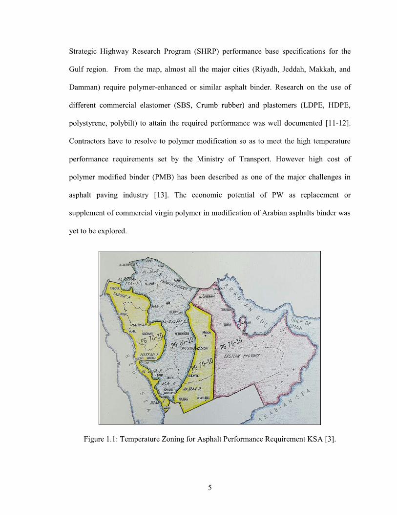
Strategic Highway Research Program (SHRP) performance base specifications for the
Gulf region. From the map, almost all the major cities (Riyadh, Jeddah, Makkah, and
Damman) require polymer-enhanced or similar asphalt binder. Research on the use of
different commercial elastomer (SBS, Crumb rubber) and plastomers (LDPE, HDPE,
polystyrene, polybilt) to attain the required performance was well documented [11-12].
Contractors have to resolve to polymer modification so as to meet the high temperature
performance requirements set by the Ministry of Transport. However high cost of
polymer modified binder (PMB) has been described as one of the major challenges in
asphalt paving industry [13]. The economic potential of PW as replacement or
supplement of commercial virgin polymer in modification of Arabian asphalts binder was
yet to be explored.
1
Figure 1.1: Temperature Zoning for Asphalt Performance Requirement KSA [3].
6
Summary: RPW have negative economic and environment impact in terms of
proper handling and disposal. High amount of the RPW is generated globally each year,
with combined annual municipal solid waste (MSW) generation of KSA exceeding
14,000,000 tones. A review on the use of recycled solid waste shows that plastic waste
constitute 10% of the bulk MSW. The RPW have potential for use in the modification of
AC. There is already a huge demand for asphalt polymer modification in KSA, due
adverse climate and increased traffic load. The RPW will be utilized together with and in
place of a virgin polymer to produce a cheaper and more durable AC for KSA climate.
7
CHAPTER 2
LITERATURE REVIEW
Introduction: The literature review is categorized into five main subheadings:
i) literature addressing asphalt binder modification for enabling improved performance in
road construction and other applications, such as roofing, and literature that aims to
improve the performance of AC by partially replacing the aggregate component of the AC
with RPW. ii) Current state of practice as regards the use of RPW in road construction
globally, and the method of RPW collection by the eastern province municipality in KAS
was also highlighted. iii) Past and current studies on polymer modified asphalt storage
stability was also reviewed. iv) Studies on AC rutting and FN test, and v) Fatigue life of
AC and related literature were finally presented.
2.1 USE OF RECYCLED PLASTIC WASTE (RPW) IN
ASPHALT CONCRETE
More than 300 Million metric tons of plastic waste (PW) was globally generated
annually as of 2014, this value is expected to keep rising [14]. Countries that has the best
recycling rate records reuse about just 50%, while 90% of the plastic waste end in
landfills in most Countries [14]. Among the high-tech recycling approaches are: Plastic-
Waste-to-Fuel via pyrolysis [15] and Plastic-Waste-to-Energy via incineration [16]. But
the major limitation of these advanced recycling options is their elimination of the plastic
8
waste without relieving the material demand of such. Thus, keeping the waste generation
and related virgin plastic production emission growing. Moreover, the Plastic-Waste-to-
Energy other disadvantage is related to the toxic emissions accompanying the combustion
of several types of plastics [17]. The other popular but low-tech recycling alternative is
the use of the recycled plastics wastes in construction or manufacturing processes instead
of the virgin type. Several among this option relieved the demand for the virgin plastic
materials at the same time disposing off the wastes.
Several research were carried out to explore the potential of PW in building and
construction applications [5, 18-19]. Polymer modified asphalt is the key component of a
high performance flexible pavement [20]. But due to the environmental and cost concern
associated with the use of virgin polymer, PW are being explored as alternative for
asphalt binder modifications [9, 21-25]. Some portion of the flexible pavement aggregate
are also being replaced with PW [26-27]. A low density AC was obtained by substituting
20% by volume of aggregate without significant loss in marshal stability [28]. Up to 30%
by volume of aggregate was replaced by low density polyethylene in dense graded
flexible pavement [29]. The recorded lightness in weight was offset by loss in indirect
tensile strength.
In past studies that explored the modification of asphalt binder using recycled
polymer waste, the optimized polymer-asphalt mixing duration was reported to be greater
than 2 hr at temperatures of 180 to 200°C [21]. When asphalt is subjected to high
temperatures for an extended period of time, such as 2 hr, it will undergo oxidation [30].
Oxidation is responsible for the degradation of certain mechanical properties of asphalt
9
due to aging. Furthermore, a particle size of 1.18 to 2.36 mm seems to be preferred when
RPW is used to partially replace AC aggregates [27, 31]. There is no experimental basis
for this selection. Therefore, this preferred size might not be optimal. Another observation
is the type of test conducted in most of the relevant studies. The current state-of-the-art
performance tests were not typically used in previous research. A thorough and high
quality study needs to be conducted in this research area.
2.1.1 RPW AS ASPHALT BINDER MODIFIER
Murphy et al. [25] used various polymers including polyethylene (PE),
polypropylene (PP), ethylene vinyl acetate (EVA), styrene butadiene styrene (SBS),
polyether polyurethane, truck tire rubber and ground rubber, as an asphalt modifier with
the intention of obtaining an appropriate blend that will exhibit similar properties as
Polyflex 75 (modified binder) and 100 penetration bitumen. Their experimental results
provided satisfying blends containing LDPE and ethyl-vinyl acetate for further
consideration because of the similarity of their properties to those of 100 penetration
bitumen and Polyflex 75.
García-Morales et al. studied the rheological characteristics and microstructure of
recycled EVA-modified bitumen [32]. Dynamic shear test was conducted in the linear
visco-elastic region. Significant increase in storage and loss moduli values were observed
at high temperature, indicating increased resistance to permanent deformation.
Furthermore, micro-structural changes were also observed through optical microscopy
and modulated differential scanning calorimetry (MDSC) for polymer content of up to
10
9% in the blends. This is related to the interaction between large swollen polymer
particles and the other constituents of the asphalt.
The effect of hydrogen-peroxide-treated (ozonized) PVC pipe waste on the
behavior of asphalt mastic has been reported [33]. Various samples were prepared from
SBS-modified (20 to 30%wt.) bitumen with varying contents of coarse and micronized
H2O2-treated PVC particulates (60-70%wt.) along with limestone dust (7-15%wt.). The
ozonized PVC waste demonstrated a better performance in terms of improved viscoelastic
properties (as indicated by dynamic mechanical analyses (DMA) and rheometer test
results). This is attributed to the lower molecular mass and rougher and porous surface
characteristics of the treated particles, as evidenced by UV-visible spectrometry and SEM
measurements, which leads to a consistent and better particle-bitumen anchorage. A roof
mastic composition of treated coarse and micronized PVC waste, isocyanate waste,
limestone dust, anti-oxidant, rosin and SBS-modified bitumen that satisfied Indian
specifications (IS 1195-90 Bitumen Mastic for Flooring) has been fully characterized.
Furthermore, the modification of an asphalt binder for roofing using PVC
packaging waste has been conducted [34]. Samples from asphalt containing (0-10%wt.
asphalt) PVC waste were subjected to low-temperature flexibility, elongation, tension,
alkali and acid resistance, softening point, ductility and penetration tests during a 12-
month aging cycle period. The results revealed positive performance improvements. This
is related to FT-IR findings that show negligible differences in the locations and
magnitudes of peaks in the absorption band between the modified and unmodified
asphalt, which implies a compatible physical interaction among the PVC waste and light
11
oil asphalt constituents. Additional microscopic images showed the emergence of a
disperse and continuous polymer-rich microstructure with increasing polymer content.
The effect of using recycled toner cartridge plastic waste on the properties and
behavior of asphalt binder has been examined [22]. The research was funded by the Texas
Department of Transportation in an attempt to improve the performance of hot mix
asphalt and facilitate the recycling of toner cartridge waste. Three test road sections
having different toner compositions were constructed at various locations. The toner level
required to achieve different superpave performance grading were established for each
type of toner waste. Bending beam rheometer results shows increased stiffness (m-value)
for the modified asphalt, thus indicating increased susceptibility to lower-temperature
cracking. A mixing time of 60-90 min was required to obtain a homogenous mix.
However, the asphalt-toner blend exhibits lower thermal storage stability.
Ho Susanna et al. performed asphalt modification using combinations of three
LDPE wax materials and three recycled LDPE materials [24]. The molecular weight and
molecular weight distribution of recycled LDPE were observed to significantly affect the
modified asphalt’s hot storage stability and behavior at low temperature. Low-molecular-
weight LDPE with wider molecular weight distributions was found to be more suited for
asphalt modification compared to LDPE with higher molecular weight and a narrower
molecular weight distribution.
An economic feasibility evaluation of the utilization and processing of mixed
plastic waste (MPW) with or without vacuum residue (VR) under conditions
characteristic of Saudi Arabia has been conducted [2]. The study established all the
12
associated costs related to the processing of MPW and conducted sensitivity and
profitability analyses. The processing of MPW with VR at a capacity of 200,000 tons per
year was found to be economically feasible under conditions found in Saudi Arabia. An
internal return rate (IRR) value of 14.6% with a corresponding payback period of
approximately 6 years and break-even capacity of 47.6% were estimated.
The feasibility and potential use of recycled waste polymer as a modifier in stone
mastic asphalt (SMA) in Ireland has been investigated [21]. The study focused on
increasing the market value of local commercially available recycled waste plastic and
providing guidelines for and insight into the use of RPW for quality road construction in
that country. Several types of RPWs were identified, including LDPE, medium-density
PE (MDPE), and HDPE, which are mainly used for packaging and plastic bottles; PVC;
PP; PET; and acrylonitrile butadiene styrene (ABS). Only three of the RWPs (PP, HDPE
and LDPE) were successfully blended with the binder. The remaining polymers were
found to be immiscible with the bitumen due to their high melting point, high density or
low surface area. A straight-grade bitumen was selected for the study. The optimized
bending time and temperature were 2.5 hr and 180°C at 4% HDPE content; this RPW
blend showed the most promising results. The RPW was found to outperform the
traditional mix when subjected to performance testing, such as wheel track and indirect
tensile fatigue tests. However, the use of virgin polymer still yields better results than the
RPW. The study recommended the blending of both RPW and virgin polymers, especially
the elastomeric type, so as to compensate for the loss of elasticity of the RPW-modified
asphalt. As with most similar studies, the mixing time of the RPW is long and could be
very costly when large quantities of bitumen are needed for road projects. The
13
morphology of the binder has not been closely examined to determine the extent to which
the RPW is blended. This could be performed with high-resolution imaging processes,
such as SEM. The above point is important in regard to analyzing the effects of time,
temperature and rate of shearing (which has not been mentioned) on the morphology. So,
for all that is observed, the increased penetration and softening point of the binder could
be mainly due to the oxidation of the binder as a result of the prolonged mixing time and
not because of the homogeneous mixing of the RPW with the binder.
In a comparative analysis of the modifying effect of reactive and non-reactive
polymers [35], the effect of recycled EVA and a combination of recycled EVA with
LDPE (EVA/LDPE) on the rheology of asphalt was reported. The recycled EVA- and
EVA/LDPE-modified asphalts show both increased losses and elastic modulii. Bitumen
modified with 5% EVA/LDPE yields the maximum linear visco-elastic moduli within a
temperature range of -10 to 50°C.
The micro-structure and properties of asphalt modified with PE waste have been
investigated [23]. The homogeneity and dispersion of the PE waste in bitumen was
improved through the addition of an organophilic Momtmorillomite (OMMT). The PE
waste was collected from domestic garbage. The FT-IR results showed no change in the
functional group of the modified asphalt, and SEM and fluorescence microscopy analyses
showed a more homogenous micro-structure due to the addition of OMMT. As a result,
an increased softening point and penetration with improved ductility were observed.
Up to 5% of 2 mm shredded LDPE collected from domestic waste has been
utilized to modify an asphalt binder [36]. The mixing of the waste and the binder was
14
performed at 165°C with a shearing speed of 3,500 rpm. Fluorescent microscopy
scanning (FMS) was employed to verify the homogeneity of the PE-modified binder.
Three factors were the main focus of the examination: temperature effects on binder
properties, the effects of the mixing duration on the binder properties, and the effects of
the PE content on the asphalt binder properties. The results from conventional asphalt
tests show slight changes in penetration and softening point values with increasing
blending temperature. Increasing the blending temperature facilitates the PE-asphalt blend
mixing, hence obtaining harder polymer-modified binder. As the PE content is increased,
the rate at which the softening point and penetration increased was lower. It was shown
that, by keeping blending time constant, the increase in PE content required higher
temperatures for the development of modified asphalt. PE-modified binders were found to
exhibit relatively lesser loss on heating, when compared to the neat asphalt binder. This
result was possible because significant proportions of the high volatile fraction of the
binder were absorbed and trapped within the swollen PE pellets.
Fang, C. et al. modify asphalt using a combination of packaging PE and rubber
powder [37]. They performed rolling thin film oven (RTFO) tests and studied the aging
mechanism using Fourier transform infrared spectroscopy (FTIR). They used rubber
powder with a fineness range of 300–600 µm and waste PE with a chip size of 1.5 cm X
2.5 cm. The polymer-asphalt blending was performed at 180°C at four different
combinations and percentages. A significant decrease in the ductility and an increase in
the softening point were observed following the RTFO aging test. However, the results
indicate changes in the ductility and softening point of modified asphalt due to the aging
of the asphalt to be less significant than that of raw asphalt. The penetration variation of
15
modified asphalt is also smaller than that of raw asphalt, which is an indication of the lack
of dependency of the penetration on the aging of modified asphalt to some extent.
Singh et al. studied the modification of asphalt using maleic anhydride and
recycled LDPE [38]. They found significant increases in the softening point and some
reduction in penetration due to modification with maleic anhydride. The difference was
conspicuous when the base bitumen was modified with higher percentages of maleic
anhydride. The viscosity of the maleated bitumen was found to be higher than that of
bitumen without maleic anhydride and thus produced improved viscoelastic properties of
the resulting blend. The recoverable blends composed of recycled LDPE and SBS
displayed satisfactory softening points and low-temperature susceptibility.
2.1.2 RPW AC MODIFICATION VIA AGGREGATE SUBSTITUTION
In a review of the use of recycled solid waste material in asphalt pavement
construction in the United Kingdom [5], a substantial proportion of the generated solid
waste plastic that could be successfully utilized as a substitute for virgin aggregate in
pavement construction was reported as not being recycled for this purpose. Several types
of plastic waste could be used as fine aggregate if they pass the standard specification test
for surface course aggregates. Recycled plastic mainly containing LDPE was used to
substitute 30% of 2.36 mm to 5 mm aggregate in a dense bituminous macadam (DBM).
This lowered the mix density by 16% and increased the mix Marshal stability by 250%.
Smaller sized LDPE (0.3-0.92 mm) was also utilized as 15% of the aggregate in asphalt
surfacing. This resulted in a higher retained stability of 15% and doubled the Marshal
quotient. However, a higher binder content is required in this situation. Positive results
16
were also reported when PVC particles were used. But only limited performance tests
were performed on AC modified using RPW aggregate. Fewer types of RWP were
utilized as aggregate substitutes.
The effect of PET on the performance of stone mastic asphalt (SMA) has been
reported [27]. Crushed PET waste 2.36 mm and smaller was incorporated into an SMA
mix to substitute 0-1%wt. of the aggregate. The stiffness of the mix decreased at a higher
PET waste content, whereas the fatigue life of the PET-modified SMA significantly
improved.
A hybrid recycled waste containing 20% nitrile rubber and 80% PE was obtained
by shred mixing (2.36 mm to 1.18 mm). The effect of the use of the waste on various
mechanical properties of the AC was investigated [31]. Mix containing 8% of the waste
by weight of the aggregate showed improved Marshal stability, Marshal quotient and
retained stability. The indirect tensile strength of the modified mix increases by up to 50%
as compared to the conventional mix. However, the modified mix exhibited a reduced
rutting tendency based on results from a wheel track test.
Local recycled plastic (RP) in corporation with recycled aggregate pavement was
utilized to investigate how to improve the efficiency and performance flexible pavement
maintenance in Algeria [39]. The RP, which is mainly composed of plastic bottles and
cable phone plugs, was obtained from a local plastic recycling company. Granular pellets
of the RP material of approximately 4 mm were utilized as a substitute of up to 8% of the
mix aggregate. However, the procedure of the asphalt mix preparation and the test
17
conducted on the prepared samples are not the current state of the art. The Marshall mix
design and test procedure employed for this study could produce misleading results.
2.2 PLASTIC WASTE USED IN ROAD CONSTRUCTION
Certain states in India have used between 10% and 15% polythene plastic waste
content to modify asphalt binder used in road construction. The available polythene waste
was estimated to cover up to 134 km span of road. An equivalent savings of 35,000 to
45,000 Indian rupees per km of road was calculated. Good initial road performance was
also reported, and improved long-term performance is also anticipated [40]. An extensive
research on the use of PW waste for road construction has made it possible for Indian
government to make it (PW) mandatory road construction material [41].
Several test roads of plastic waste modified asphalt concrete AC were constructed
in the city of Vancouver, Canada [42]. Approximately 20% of the mix proportion was
replaced with reclaimed asphalt and a wax derived from plastic waste. Various initial
benefits, such as low cost and a reduced carbon footprint, related to the mix processing
were reported. The performance results will be obtained in the near future.
2.2.1 Eastern Province Municipal Recycling Program KSA
The Eastern Province municipality in KSA has started a domestic waste recycling
program as a part of its sustainable city initiatives. The recycling program is currently
very limited and depends on sorting the domestic waste during collection using separate
trash containers as shown in Figure 2.1. The recycling program will be expanded in the
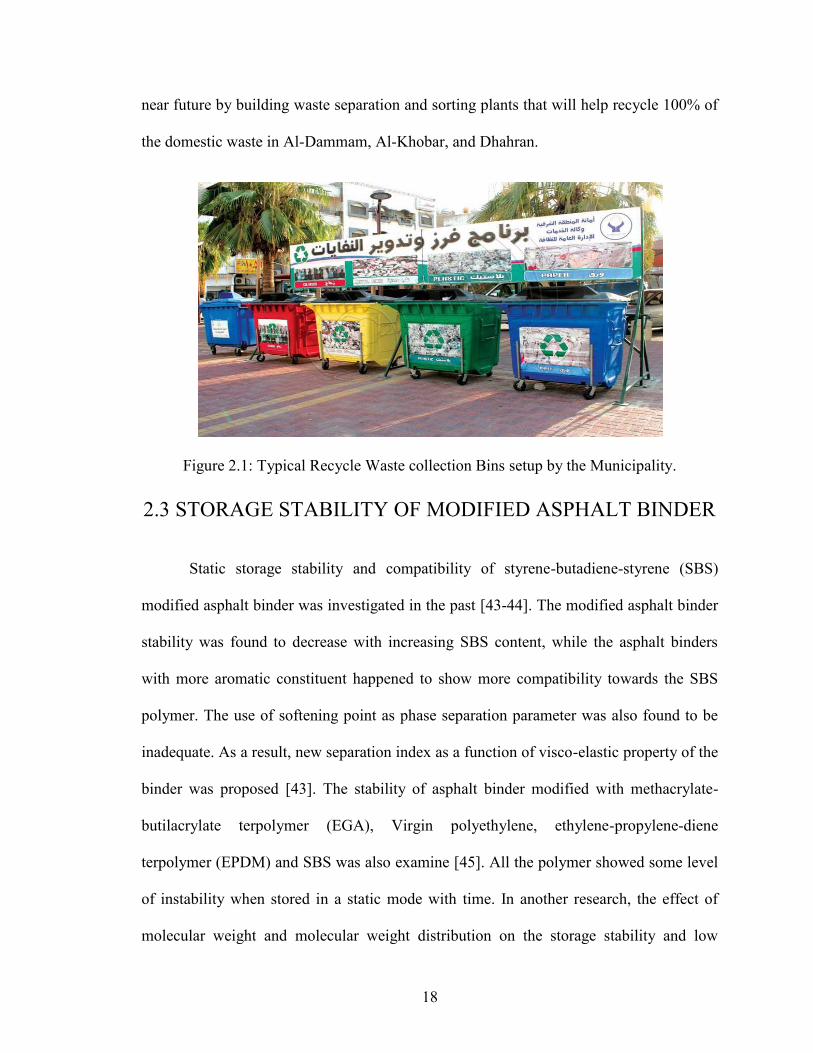
18
near future by building waste separation and sorting plants that will help recycle 100% of
the domestic waste in Al-Dammam, Al-Khobar, and Dhahran.
Figure 2.1: Typical Recycle Waste collection Bins setup by the Municipality.
2.3 STORAGE STABILITY OF MODIFIED ASPHALT BINDER
Static storage stability and compatibility of styrene-butadiene-styrene (SBS)
modified asphalt binder was investigated in the past [43-44]. The modified asphalt binder
stability was found to decrease with increasing SBS content, while the asphalt binders
with more aromatic constituent happened to show more compatibility towards the SBS
polymer. The use of softening point as phase separation parameter was also found to be
inadequate. As a result, new separation index as a function of visco-elastic property of the
binder was proposed [43]. The stability of asphalt binder modified with methacrylate-
butilacrylate terpolymer (EGA), Virgin polyethylene, ethylene-propylene-diene
terpolymer (EPDM) and SBS was also examine [45]. All the polymer showed some level
of instability when stored in a static mode with time. In another research, the effect of
molecular weight and molecular weight distribution on the storage stability and low
19
temperature properties of recycled low density polyethylene was explored [24]. Low
molecular weight LDPE with wider molecular weight distribution exhibits superior
properties than LDPE with higher molecular weight and narrow molecular weight
distribution. No specific conclusion was made about content range of recycled LDPE that
could possibly warrant stable asphalt blend. Later on, compatibility and storage stability
of a polar monomer grafted SBS modified asphalt binder was reported [46]. The polarized
SBS modified binder was found to be relatively more stable than the normal SBS
modified asphalt binder. Addition of nano-clay was also reported to improve the storage
stability of the SBS modified asphalt binder [47]. The reason given for this improvement
was not due to prevention of phase separation, but rather the settling of the clay to bottom
of the aluminum test tube. This compensates the difference in softening point that could
be observed between the top and bottom samples, which occurs due to the migration of
the SBS polymer to the surface. Hence, another reason that prompt the question of
appropriateness of the static approach of testing of modified asphalt stability arise. In
another study, effect of sulfur and base bitumen constituent on the stability of SBS
modified asphalt has been examined [48]. Even though the variously utilized type of
bitumen showed similar constituent proportions, the stability of their SBS modified
blends differ. Addition of sulfur to the SBS modified asphalt helps retards phase
separation through the formation of additional cross link within the polymer phase
network (vulcanization). The storage stability examination in all the above mentioned
studies was conducted in static mode.
The storage stability test employed by all the above mentioned studies, was based
on the the American Society for Testing and Materials standard test for possible
20
separation of polymer phase from the asphalt (ASTM D5892). Due to several questions
that this standard test could not address, it has been withdrawn since 2005. For example,
the standard specified that the sample be statically stored in a cylindrical tube within an
oven (163oC) for some time and then cool to a freezing temperature. It is then cut into
three part for the softening point of the top and bottm parts to be tested. But in reality the
polymer modified asphalt undergoes a contious agitation in the storage tank, prior to
mixing with aggregate [49]. This crutial factor, which can make or break the stability of a
given polymer in an asphalt binder was not considered by the test. The specified test
parameter (softening point) that measures the separation extent was found to be indequate
[43]. Some studies suggeted that this method exaggerates the seperaration tendency of the
modified asphalt [50]. An alternative test method that reflect actual field performance was
proposed by a National Cooperative Highway Research Program (NCHRP) research
under the Strategic Highway Research Program (SHRP), which has been evaluated by the
Federal Highway Administration (FHWA) [49]. This alternative test method for storage
stability was employed in this study.
2.4 RUTTING AND FLOW NUMBER TEST OF ASPHALT
CONCRETE
Dynamic creep load test was found to correlate excellently with the rutting
performance of asphalt mixtures [51]. The three main stages utilized in describing and
modeling the permanent deformation of the asphalt material was earlier verified through
field and laboratory studies [52]. Repeated load testing is now part of asphalt mix simple
performance tests as Flow Number (FN) test [53]. This was the result of series of research
21
carried out under the National Cooperative Highway Research Program [51]. The FN test
is being used as a measure of rutting resistance of asphalt pavement mixtures for quality
control and assurance [54]. The asphalt repeated load test was also adopted as part of a
provisional standard by American Association of State Highway and Transportation
Officials as AASHTO: TP 79. Research were carried out to further standardize and
accommodate various asphalt mix type such as warm mix asphalt [55]. The standardized
test has accounted for different source of variation like testing loads, aggregate sizes,
sample preparation for laboratory test specimens etc. However, there are still issues which
are yet to be addressed, making it the focus of research in recent years.
Previous studies have identified some flaws of the FN test, resulting in
inconsistent FN values, and proposed possible solutions [53, 56]. The inconsistency was
found to be as a result of permanent strain data fluctuation, due to electric noise and
elastic recovery property in case of rubber mix [53]. A simple stepwise approach that
rearrange the permanent deformation curve (PDC) data increasingly was proposed [56].
Fitting the PDC data in to Francken model (FM) prior to FN estimation was
recommended as the best alternative [53]. The later approach was ultimately and widely
accepted as it is currently part of the AASHTO TP 79 standard. Further studies on the FN
test include correlating the FN with secondary strain rate, in an attempt to minimize the
test duration [57]. Genetic programming coupled with simulated annealing, multiple least
square regression and support vector machine were used to modeled the FN of Marshall
asphalt mixture test specimens [58-59]. Superpave asphalt mix volumetric parameters
were also utilized as FN predictors [60]. But not all of these previous studies conducted
were based on the current standardized test. Almost all of these research were conducted
22
on some old data base, that was acquired prior to the adaptation of the FN as a standard
test, which was drafted and activated in 2009.
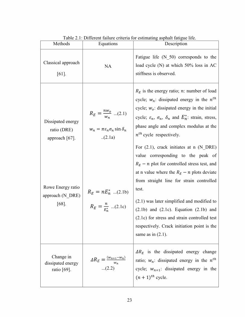
2.5 FATIGUE LIFE (FL) OF ASPHALT CONCRETE
The existing major standard methods for estimating the fatigue life of asphalt
concrete (AC) are performed at constant temperature, continuous and constant load
frequency [61-62]. Table 2.1 list the widely employed failure criteria for analyzing
fatigue test data. The standard AC fatigue test is conducted on a 50 mm thick by 63 mm
wide by 380 mm long AC beam, loaded at third points and subjected to repeated flexural
bending (10 Hz), under a constant stress or strain until failure [61].
The traditional method of 50% stiffness loss fatigue life (N_50), the Rowe energy ratio
approach (N_DRE) and the viscoelastic continuum damage approach (VECD) were
compared [63]. Both N_50 and VECD fatigue life were found to be less than the fatigue
life estimated by N_DRE approach. Thermo-mechanical fatigue life prediction model of
cement asphalt mortar was presented in [64]. The Combined effect of loading frequency,
temperature and stress level on the indirect tensile stress fatigue life of AC was
investigated [65]. The effect of recycled asphalt pavement (RAP) on the fatigue life of
asphalt concrete (AC) and asphalt binder was also investigated [66]. The RAP has a
positive and negative impact on the fatigue life of the AC and the binder respectively.
23
Table 2.1: Different failure criteria for estimating asphalt fatigue life Table 2.1: Different failure criteria for estimating asphalt fatigue life.
Methods Equations Description
Classical approach
[61]. NA
Fatigue life (N_50) corresponds to the
load cycle (N) at which 50% loss in AC
stiffness is observed.
Dissipated energy
ratio (DRE)
approach [67].
Rowe Energy ratio
approach (N_DRE)
[68].
...(2.1)
..(2.1a)
...(2.1b)
...(2.1c)
is the energy ratio; : number of load
cycle; : dissipated energy in the
cycle; : dissipated energy in the initial
cycle; , , and : strain, stress,
phase angle and complex modulus at the
cycle respectively.
For (2.1), crack initiates at n (N_DRE)
value corresponding to the peak of
plot for controlled stress test, and
at n value where the plots deviate
from straight line for strain controlled
test.
(2.1) was later simplified and modified to
(2.1b) and (2.1c). Equation (2.1b) and
(2.1c) for stress and strain controlled test
respectively. Crack initiation point is the
same as in (2.1).
Change in dissipated energy
ratio [69].
...(2.2)
is the dissipated energy change
ratio; : dissipated energy in the
cycle; : dissipated energy in the
cycle.
24
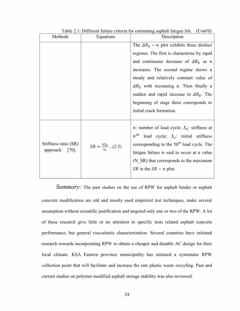
Table 2.1: Different failure criteria for estimating asphalt fatigue life. Methods Equations Description
The plot exhibits three distinct
regimes. The first is characterise by rapid
and continuous decrease of as n
increases. The second regime shows a
steady and relatively constant value of
with increasing n. Then finally a
sudden and rapid increase in . The
beginning of stage three corresponds to
initial crack formation.
Stiffness ratio (SR) approach [70].
...(2.3)
: number of load cycle; : stiffness at
load cycle; : initial stiffness
corresponding to the 50th load cycle. The
fatigue failure is said to occur at n value
(N_SR) that corresponds to the maximum
in the plot.
Summary: The past studies on the use of RPW for asphalt binder or asphalt
concrete modification are old and mostly used empirical test techniques, make several
assumption without scientific justification and targeted only one or two of the RPW. A lot
of these research give little or no attention to specific tests related asphalt concrete
performance, but general viscoelastic characterization. Several countries have initiated
research towards incorporating RPW to obtain a cheaper and durable AC design for their
local climate. KSA Eastern province municipality has initiated a systematic RPW
collection point that will facilitate and increase the rate plastic waste recycling. Past and
current studies on polymer modified asphalt storage stability was also reviewed.
(Cont'd)
25
CHAPTER 3
METHODOLOGY
Introduction: This chapter describes the methodology followed in carrying
out the various tasks involved in this research. The study has been divided into three
phases. The first phase addresses the identification of RPWs that can be used in asphalt
modification or replacement of aggregate, followed by the evaluation of RPW-modified
asphalts. Different potential RPWs will be screened and selected based on thermal and
rheological techniques. The second phase involves analysis of the performance and
mechanical properties of RPW-modified AC mixtures composed of both pure binder and
pure RWP or blended modified asphalt binder. The third phase includes data analyses and
reporting. The overall work sequence and content has been summarized in the work flow
chart a shown Figure 3.1. The RPW modified asphalt test experimental design was
presented. The RPW-AC mix optimization and performance evaluation guide was also
shown. The detail description of the test and analysis methods employed has been
provided in the subsequent subheadings. Details of the AC mechanic-empirical
performance modeling method adopted was also described.
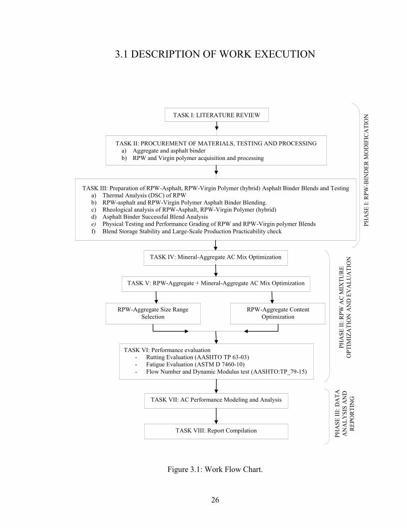
26
3.1 DESCRIPTION OF WORK EXECUTION
Figure 3.1: Work Flow Chart.
TASK I: LITERATURE REVIEW
TASK II: PROCUREMENT OF MATERIALS, TESTING AND PROCESSING a) Aggregate and asphalt binder b) RPW and Virgin polymer acquisition and processing
TASK III: Preparation of RPW-Asphalt, RPW-Virgin Polymer (hybrid) Asphalt Binder Blends and Testing a) Thermal Analysis (DSC) of RPW b) RPW-asphalt and RPW-Virgin Polymer Asphalt Binder Blending. c) Rheological analysis of RPW-Asphalt, RPW-Virgin Polymer (hybrid) d) Asphalt Binder Successful Blend Analysis e) Physical Testing and Performance Grading of RPW and RPW-Virgin polymer Blends f) Blend Storage Stability and Large-Scale Production Practicability check
PHA
SE II
: RPW
AC
MIX
TUR
E O
PTIM
IZA
TIO
N A
ND
EV
ALU
ATI
ON
TASK IV: Mineral-Aggregate AC Mix Optimization
TASK V: RPW-Aggregate + Mineral-Aggregate AC Mix Optimization
TASK VI: Performance evaluation - Rutting Evaluation (AASHTO TP 63-03) - Fatigue Evaluation (ASTM D 7460-10) - Flow Number and Dynamic Modulus test (AASHTO:TP_79-15)
TASK VII: AC Performance Modeling and Analysis
PHA
SE II
I: D
ATA
A
NA
LYSI
S A
ND
R
EPO
RTI
NG
TASK VIII: Report Compilation
RPW-Aggregate Size Range Selection
RPW-Aggregate Content Optimization
PHA
SE I:
RPW
-BIN
DER
MO
DIF
ICA
TIO
N
27
3.1.1 PHASE I: RPW BINDER MODIFICATION
The tasks for each phase of the research are listed under the appropriate heading.
An initial set of sub-tasks of some of the main tasks are carried out concurrently.
3.1.1.1 TASK I: LITERATURE REVIEW
A thorough literature review of current and past research related to the use of
RPW for asphalt modification has been carried out. The current practices and approaches
related to research on RPW asphalt concrete from developed countries were also
documented.
3.1.1.2 TASK II: PROCUREMENT OF MATERIALS, TESTING AND
PROCESSING
A. Aggregate and Asphalt Binder: A neat asphalt binder, which was collected from
local refineries, was used in this study. A common and local type of aggregate were
also collected from the nearest quarry.
The aggregate was analyzed for conformity with ASTM specifications for
aggregates to be used for road construction. ASTM D1241-07: (Specific Gravity,
Water Absorption, Soundness, angularity and L.A. Abrasion tests). The asphalt
binder was characterized using the asphalt the Performance Grade tests (AASHTO
MP-19) and (AASHTO TP-70).
B. RPW and Virgin Polymer Acquisition and Processing:
28
Local plastic waste were identified and handpicked from municipal waste
collection program. These wastes were then processed for easier use. Virgin
polymers, which include plastomeric Polybilt (PB) and elastomeric styrene
butadiene styrene (SBS), were acquired from commercial source. The processing
involves the following:
a. Shredding and Grinding: the RPWs were shredded, and some amount of the RPW
was subjected to grinding using special plastic shredding and grinding machines.
For example, RLDPE and RHDPE waste must be ground to the desirable size,
depending on whether it will be used for blending with asphalt binder (fine) or for
modifying the aggregate composition of asphalt concrete (AC).
b. Cleaning: washing and drying for the removal of organic materials.
Classification of the RPW into two groups according to the melting point: the first
group with low melting points were selected for asphalt modification, whereas the second
group were examined for potential use as aggregates replacement. Thermal analysis and
characterization techniques was employed for this purpose. Differential scanning
Calorimetry (DSC) was used to determine the melting point, and, accordingly, potential
RPW candidates for asphalt modification as well as for aggregate substitution were
identified.
3.1.1.3 Task III: Preparation of RPW-Asphalt Binder, RPW-Virgin
Polymer (hybrid) Asphalt Binder Blends and Testing
RPWs with recycle labels 2, 4 and 5, which are RHDPE, RLDPE and RPP,
respectively, will be the main focus in this task.
29
A. A differential scanning calorimeter (DSC) Q1000 was used to determine the
melting point of the RPWs.
B. An ARES rheometer was used to determine the viscoelastic properties of the
RPWs and virgin polymers modified asphalt binders.
C. RPW-asphalt and RPW-Virgin Polymer Asphalt Binder Blending.
For this particular task, a special air-tight and high-shear mixer (blender) with a
shear speed of up to 5,000 rpm was acquired. This was necessary because most
RPW cannot be easily blended with asphalt binder.
Preliminary Mixing of the RPW with the Binder: Various mixing duration for each
type of RPW with the asphalt binder at temperatures above the RPW melting point
was explored to determine the optimal mixing duration.
D. Asphalt Binder Successful Blend Analysis: samples prepared under various
mixing were subjected to dynamic shear rheological (AASHTO PP6) and
rotational viscosity (ASTM D 4402) tests. These results were plotted against the
mixing duration for analysis.
E. Physical Testing and Performance Grading of RPW and RPW-Virgin polymer
Blends
The viscoelastic performance properties of asphalt blends with various RPW
contents (and in combination with a visco-elastic or viscos-plastic virgin
polymer) was investigated. Table 3.1 shows the experimental design that was
followed. The series of tests that were conducted are listed below.
1) Rotational viscosity test (ASTM D 4402)
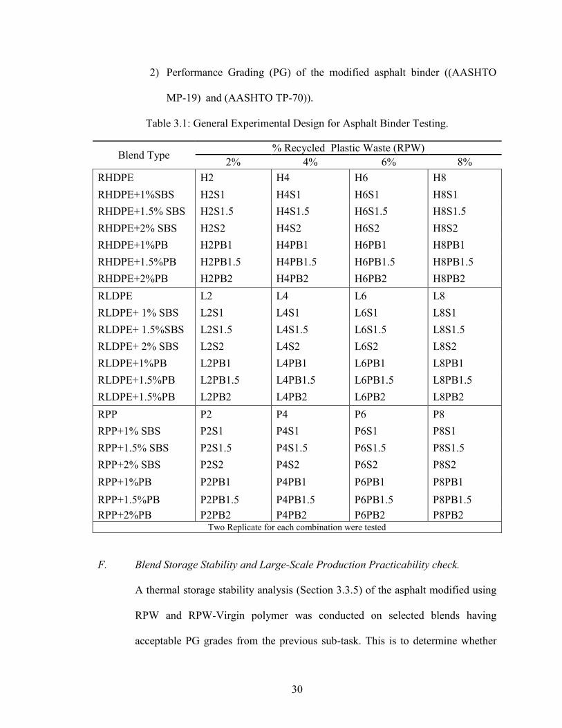
30
2) Performance Grading (PG) of the modified asphalt binder ((AASHTO
MP-19) and (AASHTO TP-70)).
Table 3.1: General Experimental Design for Asphalt Binder Testing.
Blend Type % Recycled Plastic Waste (RPW)
2% 4% 6% 8% RHDPE H2 H4 H6 H8 RHDPE+1%SBS H2S1 H4S1 H6S1 H8S1 RHDPE+1.5% SBS H2S1.5 H4S1.5 H6S1.5 H8S1.5 RHDPE+2% SBS H2S2 H4S2 H6S2 H8S2 RHDPE+1%PB H2PB1 H4PB1 H6PB1 H8PB1 RHDPE+1.5%PB H2PB1.5 H4PB1.5 H6PB1.5 H8PB1.5 RHDPE+2%PB H2PB2 H4PB2 H6PB2 H8PB2 RLDPE L2 L4 L6 L8 RLDPE+ 1% SBS L2S1 L4S1 L6S1 L8S1 RLDPE+ 1.5%SBS L2S1.5 L4S1.5 L6S1.5 L8S1.5 RLDPE+ 2% SBS L2S2 L4S2 L6S2 L8S2 RLDPE+1%PB L2PB1 L4PB1 L6PB1 L8PB1 RLDPE+1.5%PB L2PB1.5 L4PB1.5 L6PB1.5 L8PB1.5 RLDPE+1.5%PB L2PB2 L4PB2 L6PB2 L8PB2 RPP P2 P4 P6 P8 RPP+1% SBS P2S1 P4S1 P6S1 P8S1 RPP+1.5% SBS P2S1.5 P4S1.5 P6S1.5 P8S1.5 RPP+2% SBS P2S2 P4S2 P6S2 P8S2 RPP+1%PB P2PB1 P4PB1 P6PB1 P8PB1 RPP+1.5%PB P2PB1.5 P4PB1.5 P6PB1.5 P8PB1.5 RPP+2%PB P2PB2 P4PB2 P6PB2 P8PB2
Two Replicate for each combination were tested
F. Blend Storage Stability and Large-Scale Production Practicability check.
A thermal storage stability analysis (Section 3.3.5) of the asphalt modified using
RPW and RPW-Virgin polymer was conducted on selected blends having
acceptable PG grades from the previous sub-task. This is to determine whether
31
the minimum storage stability level is achieved. The obtained results served as a
basis for the appropriate use and recommendation of the specific RPW used in
the asphalt binder modification.
3.1.2 PHASE II: RPW AC MIXTURE OPTIMIZATION AND
EVALUATION
RPWs with recycle labels of 1, 2, 3, 4, 5 and 6, namely, recycled Polyethylene
recycled Terephthalate (RPET), recycled High density polyethylene (RHDPE), polyvinyl
chloride (RPVC), recycled low density polyethylene (RLDPE), recycled polypropylene
(RPP), and recycled polystyrene (RPS), were utilized in the following tasks.
3.1.2.1 Task IV: Virgin Aggregate Asphalt Concrete Mix Optimization
Asphalt concrete mixtures were designed and prepared for the control binder and
nine selected modified binders: RHDPE, RLDPE, RPP, RHDPE+SBS, RLDPE+SBS,
RPP+SBS, RHDPE+PB, RLDPE+PB, and RPP+PB. Modified binders that have the
required PG will be selected from Phase I. The AC mixtures were prepared following the
superpave volumetric mix design [71], and the optimal binder content are determined in
each case which were then adopted in the next subtask. The first two columns of Table
3.2 showed the various mixtures to be designed.
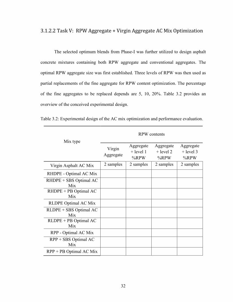
32
3.1.2.2 Task V: RPW Aggregate + Virgin Aggregate AC Mix Optimization
The selected optimum blends from Phase-I was further utilized to design asphalt
concrete mixtures containing both RPW aggregate and conventional aggregates. The
optimal RPW aggregate size was first established. Three levels of RPW was then used as
partial replacements of the fine aggregate for RPW content optimization. The percentage
of the fine aggregates to be replaced depends are 5, 10, 20%. Table 3.2 provides an
overview of the conceived experimental design.
Table 3.2: Experimental design of the AC mix optimization and performance evaluation.
Mix type
RPW contents
Virgin Aggregate
Aggregate + level 1 %RPW
Aggregate + level 2 %RPW
Aggregate + level 3 %RPW
Virgin Asphalt AC Mix 2 samples 2 samples 2 samples 2 samples
RHDPE - Optimal AC Mix
RHDPE + SBS Optimal AC Mix
RHDPE + PB Optimal AC Mix
RLDPE Optimal AC Mix
RLDPE + SBS Optimal AC Mix
RLDPE + PB Optimal AC Mix
RPP - Optimal AC Mix
RPP + SBS Optimal AC Mix
RPP + PB Optimal AC Mix
33
3.1.2.3 Task VI: Performance evaluation
Fatigue and Rutting Performance Evaluation of the Most Prominent Mixtures:
Test samples for the various successful mixtures shown in Table 3.2 were prepared and
tested using the following tests:
- Standard Test Method for Determining the Rutting Susceptibility of Asphalt
Paving Mixtures Using the Asphalt Pavement Analyzer (APA) (AASHTO TP
63-03)
- Standard Test Method for Determining Fatigue Failure of Compacted Asphalt
Concrete Subjected to Repeated Flexural Bending (ASTM D7460 - 10)
- Superpave Asphalt Mix Performance Tester (AMPT) for determining the
dynamic modulus, flow time and flow number tests.
3.1.3 PHASE III: DATA ANALYSIS AND REPORTING
3.1.3.1 Task VII: Results Analysis and AC Performance Modeling
The results from the Superpave asphalt mix performance testing (AMPT) was
utilized to simulate the service rutting and fatigue performance of the RPW-modified
hybrid asphalt concrete mix using Finite Element based Mechanistic Empirical technique.
The measured rutting and fatigue performance from Task VI is compared to the modeled
service performance. The economic feasibility of developing the modified AC mix in
terms of the costs and enhanced service life of the asphalt concrete structures was also
assessed.
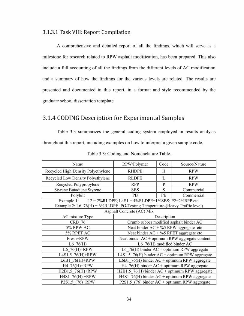
34
3.1.3.1 Task VIII: Report Compilation
A comprehensive and detailed report of all the findings, which will serve as a
milestone for research related to RPW asphalt modification, has been prepared. This also
include a full accounting of all the findings from the different levels of AC modification
and a summary of how the findings for the various levels are related. The results are
presented and documented in this report, in a format and style recommended by the
graduate school dissertation template.
3.1.4 CODING Description for Experimental Samples
Table 3.3 summarizes the general coding system employed in results analysis
throughout this report, including examples on how to interpret a given sample code.
Table 3.3: Coding and Nomenclature Table.
Name RPW/Polymer Code Source/Nature Recycled High Density Polyethylene RHDPE H RPW Recycled Low Density Polyethylene RLDPE L RPW
Recycled Polypropylene RPP P RPW Styrene Butadiene Styrene SBS S Commercial
Polybilt PB PB Commercial Example 1: L2 = 2%RLDPE; L4S1 = 4%RLDPE+1%SBS; P2=2%RPP etc.
Example 2: L6_76(H) = 6%RLDPE_PG-Testing Temperature-(Heavy Traffic level) Asphalt Concrete (AC) Mix
AC mixture Type Description CRB_76 Crumb rubber modified asphalt binder AC
5% RPW AC Neat binder AC + %5 RPW aggregate etc 5% RPET AC Neat binder AC + %5 RPET aggregate etc Fresh+RPW Neat binder AC + optimum RPW aggregate content L6_76(H) L6_76(H) modified binder AC
L6_76(H)+RPW L6_76(H) binder AC + optimum RPW aggregate L4S1.5_76(H)+RPW L4S1.5_76(H) binder AC + optimum RPW aggregate L6B1_76(H)+RPW L6B1_76(H) binder AC + optimum RPW aggregate
H4_76(H)+RPW H4_76(H) binder AC + optimum RPW aggregate H2B1.5_76(H)+RPW H2B1.5_76(H) binder AC + optimum RPW aggregate H4S1_76(H) +RPW H4S1_76(H) binder AC + optimum RPW aggregate P2S1.5_(76)+RPW P2S1.5_(76) binder AC + optimum RPW aggregate
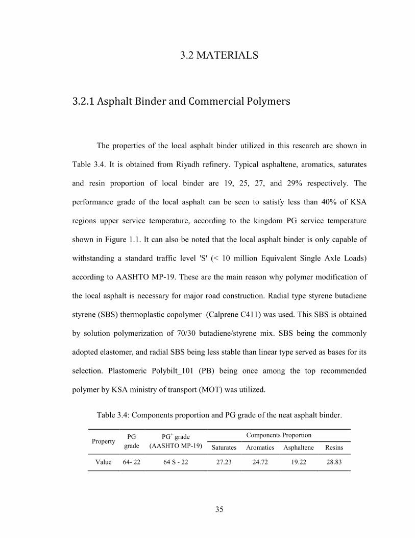
35
3.2 MATERIALS
3.2.1 Asphalt Binder and Commercial Polymers
The properties of the local asphalt binder utilized in this research are shown in
Table 3.4. It is obtained from Riyadh refinery. Typical asphaltene, aromatics, saturates
and resin proportion of local binder are 19, 25, 27, and 29% respectively. The
performance grade of the local asphalt can be seen to satisfy less than 40% of KSA
regions upper service temperature, according to the kingdom PG service temperature
shown in Figure 1.1. It can also be noted that the local asphalt binder is only capable of
withstanding a standard traffic level 'S' (< 10 million Equivalent Single Axle Loads)
according to AASHTO MP-19. These are the main reason why polymer modification of
the local asphalt is necessary for major road construction. Radial type styrene butadiene
styrene (SBS) thermoplastic copolymer (Calprene C411) was used. This SBS is obtained
by solution polymerization of 70/30 butadiene/styrene mix. SBS being the commonly
adopted elastomer, and radial SBS being less stable than linear type served as bases for its
selection. Plastomeric Polybilt_101 (PB) being once among the top recommended
polymer by KSA ministry of transport (MOT) was utilized.
Table 3.4: Components proportion and PG grade of the neat asphalt binder.
Property PG
grade PG+ grade
(AASHTO MP-19) Components Proportion
Saturates Aromatics Asphaltene Resins
Value 64- 22 64 S - 22 27.23 24.72 19.22 28.83
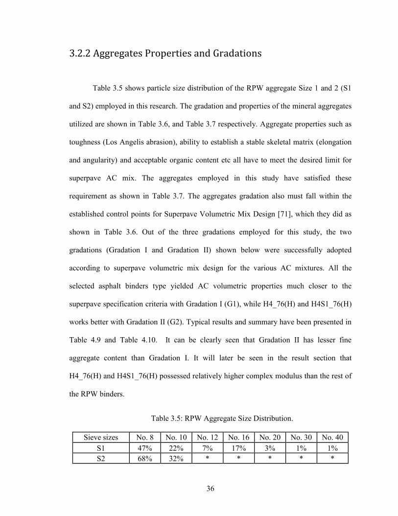
36
3.2.2 Aggregates Properties and Gradations
Table 3.5 shows particle size distribution of the RPW aggregate Size 1 and 2 (S1
and S2) employed in this research. The gradation and properties of the mineral aggregates
utilized are shown in Table 3.6, and Table 3.7 respectively. Aggregate properties such as
toughness (Los Angelis abrasion), ability to establish a stable skeletal matrix (elongation
and angularity) and acceptable organic content etc all have to meet the desired limit for
superpave AC mix. The aggregates employed in this study have satisfied these
requirement as shown in Table 3.7. The aggregates gradation also must fall within the
established control points for Superpave Volumetric Mix Design [71], which they did as
shown in Table 3.6. Out of the three gradations employed for this study, the two
gradations (Gradation I and Gradation II) shown below were successfully adopted
according to superpave volumetric mix design for the various AC mixtures. All the
selected asphalt binders type yielded AC volumetric properties much closer to the
superpave specification criteria with Gradation I (G1), while H4_76(H) and H4S1_76(H)
works better with Gradation II (G2). Typical results and summary have been presented in
Table 4.9 and Table 4.10. It can be clearly seen that Gradation II has lesser fine
aggregate content than Gradation I. It will later be seen in the result section that
H4_76(H) and H4S1_76(H) possessed relatively higher complex modulus than the rest of
the RPW binders.
Table 3.5: RPW Aggregate Size Distribution.
Sieve sizes No. 8 No. 10 No. 12 No. 16 No. 20 No. 30 No. 40 S1 47% 22% 7% 17% 3% 1% 1% S2 68% 32% * * * * *
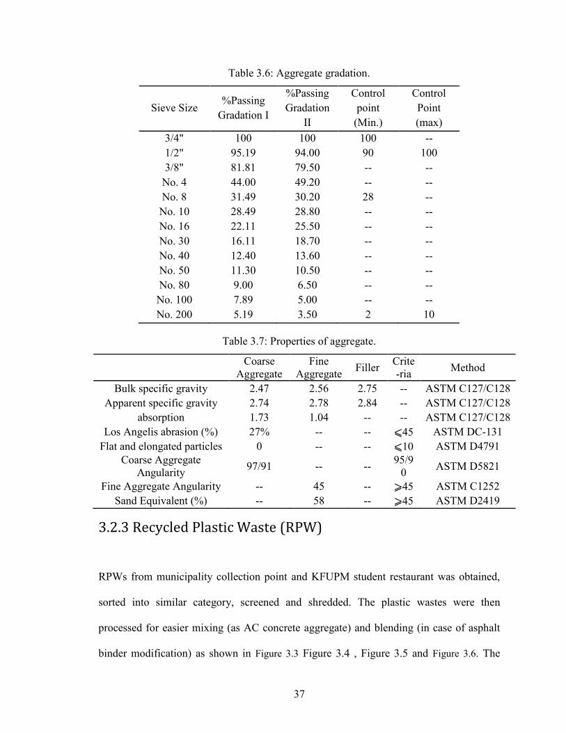
37
Table 3.6: Aggregate gradation.
Sieve Size %Passing
Gradation I
%Passing Gradation
II
Control point
(Min.)
Control Point (max)
3/4" 100 100 100 -- 1/2" 95.19 94.00 90 100 3/8" 81.81 79.50 -- --
No. 4 44.00 49.20 -- -- No. 8 31.49 30.20 28 -- No. 10 28.49 28.80 -- -- No. 16 22.11 25.50 -- -- No. 30 16.11 18.70 -- -- No. 40 12.40 13.60 -- -- No. 50 11.30 10.50 -- -- No. 80 9.00 6.50 -- -- No. 100 7.89 5.00 -- -- No. 200 5.19 3.50 2 10
Table 3.7: Properties of aggregate.
Coarse Aggregate
Fine Aggregate Filler Crite
-ria Method
Bulk specific gravity 2.47 2.56 2.75 -- ASTM C127/C128 Apparent specific gravity 2.74 2.78 2.84 -- ASTM C127/C128
absorption 1.73 1.04 -- -- ASTM C127/C128 Los Angelis abrasion (%) 27% -- -- ⩽45 ASTM DC-131
Flat and elongated particles 0 -- -- ⩽10 ASTM D4791 Coarse Aggregate
Angularity 97/91 -- -- 95/90
ASTM D5821
Fine Aggregate Angularity -- 45 -- ⩾45 ASTM C1252 Sand Equivalent (%) -- 58 -- ⩾45 ASTM D2419
3.2.3 Recycled Plastic Waste (RPW)
RPWs from municipality collection point and KFUPM student restaurant was obtained,
sorted into similar category, screened and shredded. The plastic wastes were then
processed for easier mixing (as AC concrete aggregate) and blending (in case of asphalt
binder modification) as shown in Figure 3.3 Figure 3.4 , Figure 3.5 and Figure 3.6. The
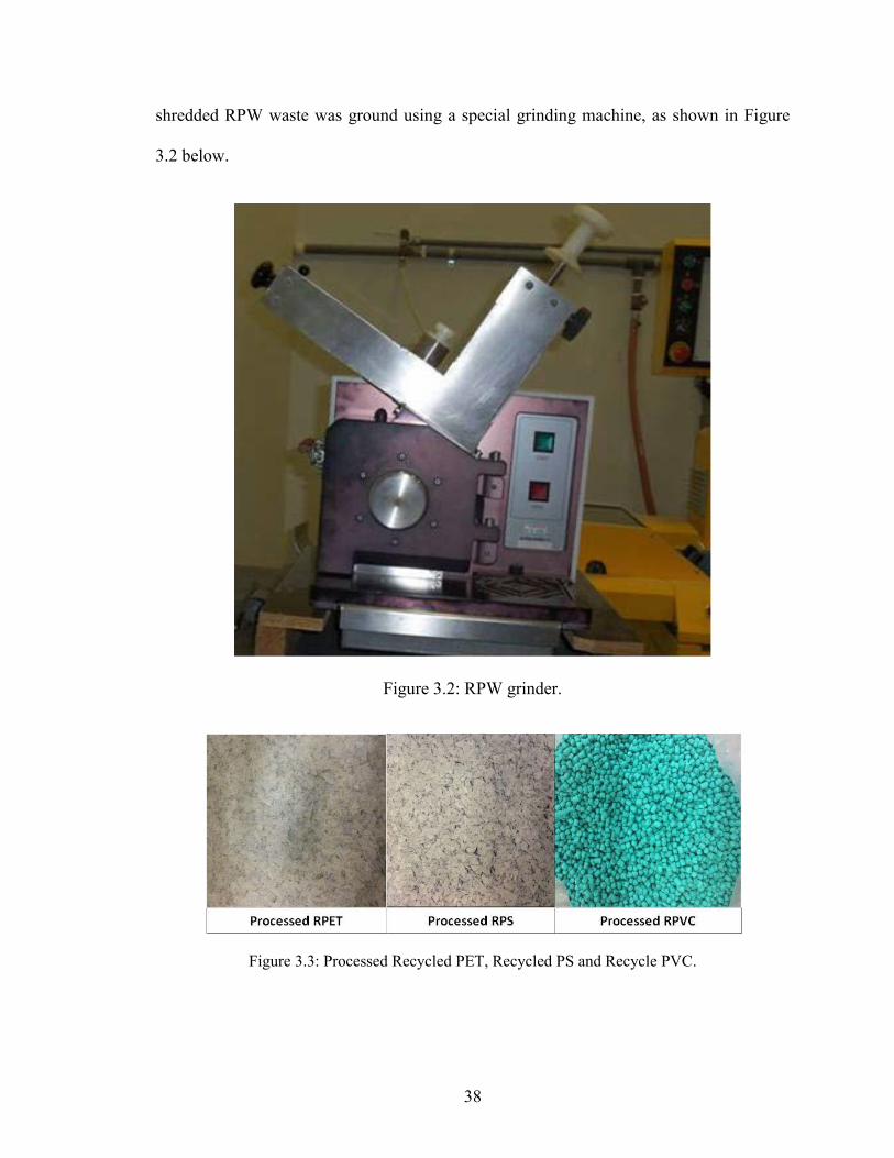
38
shredded RPW waste was ground using a special grinding machine, as shown in Figure
3.2 below.
Figure 3.2: RPW grinder.
Figure 3.3: Processed Recycled PET, Recycled PS and Recycle PVC.
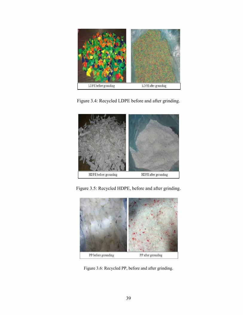
39
Figure 3.4: Recycled LDPE before and after grinding.
Figure 3.5: Recycled HDPE, before and after grinding.
Figure 3.6: Recycled PP, before and after grinding.
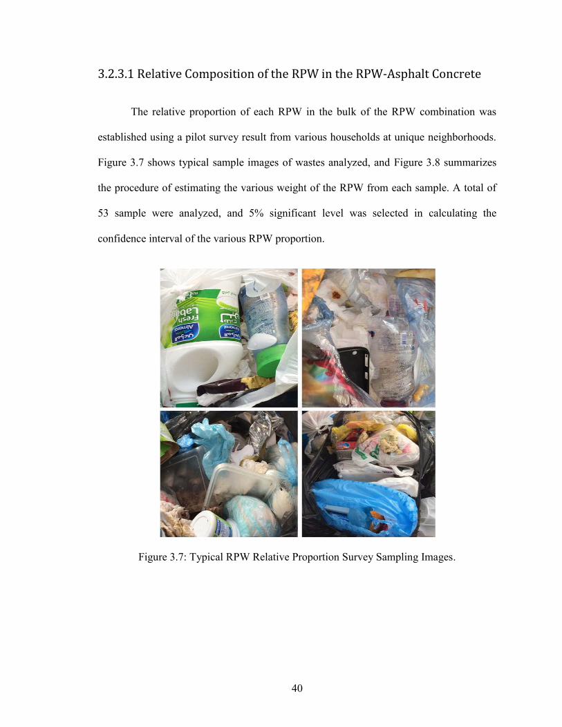
40
3.2.3.1 Relative Composition of the RPW in the RPW-Asphalt Concrete
The relative proportion of each RPW in the bulk of the RPW combination was
established using a pilot survey result from various households at unique neighborhoods.
Figure 3.7 shows typical sample images of wastes analyzed, and Figure 3.8 summarizes
the procedure of estimating the various weight of the RPW from each sample. A total of
53 sample were analyzed, and 5% significant level was selected in calculating the
confidence interval of the various RPW proportion.
Figure 3.7: Typical RPW Relative Proportion Survey Sampling Images.
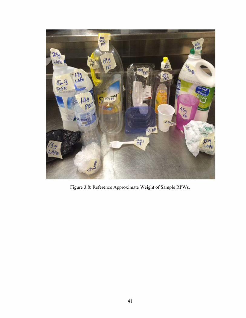
41
Figure 3.8: Reference Approximate Weight of Sample RPWs.
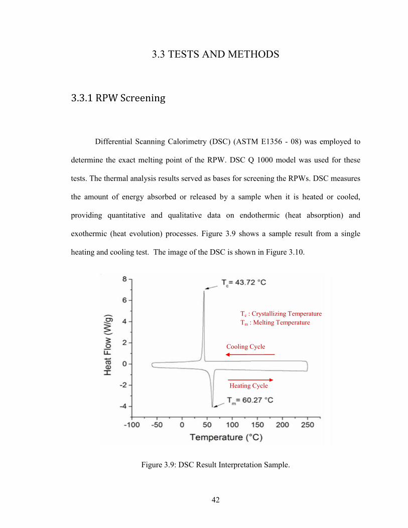
42
3.3 TESTS AND METHODS
3.3.1 RPW Screening
Differential Scanning Calorimetry (DSC) (ASTM E1356 - 08) was employed to
determine the exact melting point of the RPW. DSC Q 1000 model was used for these
tests. The thermal analysis results served as bases for screening the RPWs. DSC measures
the amount of energy absorbed or released by a sample when it is heated or cooled,
providing quantitative and qualitative data on endothermic (heat absorption) and
exothermic (heat evolution) processes. Figure 3.9 shows a sample result from a single
heating and cooling test. The image of the DSC is shown in Figure 3.10.
Figure 3.9: DSC Result Interpretation Sample.
Cooling Cycle
Heating Cycle
Tc : Crystallizing Temperature Tm : Melting Temperature
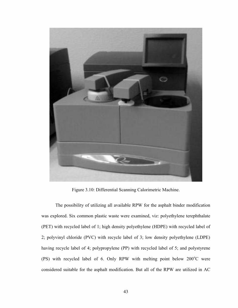
43
Figure 3.10: Differential Scanning Calorimetric Machine.
The possibility of utilizing all available RPW for the asphalt binder modification
was explored. Six common plastic waste were examined, viz: polyethylene terephthalate
(PET) with recycled label of 1; high density polyethylene (HDPE) with recycled label of
2; polyvinyl chloride (PVC) with recycle label of 3; low density polyethylene (LDPE)
having recycle label of 4; polypropylene (PP) with recycled label of 5; and polystyrene
(PS) with recycled label of 6. Only RPW with melting point below 200oC were
considered suitable for the asphalt modification. But all of the RPW are utilized in AC
44
modification as aggregate substitute. The selectiveness in case of binder modification is
purely based on the asphalt binder characteristics. When asphalt is subjected to high
temperatures for an extended period of time, it will undergo oxidation [30]. Oxidation
leads to aging of the asphalt, and aging is responsible for the degradation of vital
properties of asphalt. But in the case of AC, the there is no need for the RPW to melt in
the mix. So all the RPW can be employed in the AC modification via aggregate
substitution.
3.3.2 Optimization of RPW-Asphalt Blending Duration
The RLDPE modified asphalt was obtained by hot blending both asphalt and the recycled
plastic at 160oC and around 5000 rpm shearing speed. The blend is first placed in an oven
at 160oC inside a sealed can, for 1 hr. Rotational viscosity test and dynamic shear
rheometer test samples were obtained after 10 minutes blending time interval. The mixing
was continued for up to 50 minutes. Figure 4.7 and Figure 4.8 shows the results.
The RHDPE and RPP modified asphalt were obtained by hot blending the asphalt and the
recycled polymers at 180oC and 190oC respectively. The shearing speed of blender is
about 5000 rpm. The blends are first placed in an oven at 160oC inside a sealed can, for 1
hr. Rotational viscosity test and dynamic shear rheometer test samples were obtained after
10 minutes blending time interval. The mixing was continued for up to 70 minutes.
Figure 4.7 and Figure 4.9 showed the plots of the results.
45
3.3.3 RPW-Asphalt Blending
A customized air-tight and high shear blender shown in Figure 3.11 was employed
for the RPW-Asphalt blending. The blender can reach shearing speed up to 9000 rpm, and
a temperature of up to 500oC. The air tightness was to minimize or eliminate the
oxidation of the blended RPW-asphalt during mixing at high temperature in the presence
of air. 500 g of liquid asphalt was manually mixed with appropriate amount of RPW
(RPP, RLDPE, or RHDPE), SBS/PB, or combination of both inside a 1000 ml metallic
can. The can was sealed with aluminum foil, stored inside an oven at 160oC for an hour to
soften the added RPW, SBS/PB or both. The can was put inside a customized high shear
blender at the appropriate blending temperature (Table 4.1), the mixture was then shear-
blended at 5000 rpm for the applicable time (Table 4.1). The blending duration is 1 hour
if the RPW requires less than 1 hour and is in combination with SBS.
3.3.4 Asphalt Performance Grading
DV-II Brookfield viscometer was employed to measure the RPWs modified
asphalt viscosities (ASTM D4402). RPW-modified asphalts were subjected to a short
term aging test (AASHTO T 240 or ASTM D2872) as per AASHTO PG requirements
(AASHTO M 332-14). Dynamic shear analysis and MSCR tests were conducted on the
modified asphalt using TA CSAII Dynamic Shear Rheometer (DSR) (AASHTO M 332-
14, AASHTO TP 70-11). Further details of the tests and equipments involved in the
performance grading of the modified asphalt binder are shown in the following sub-
headings.
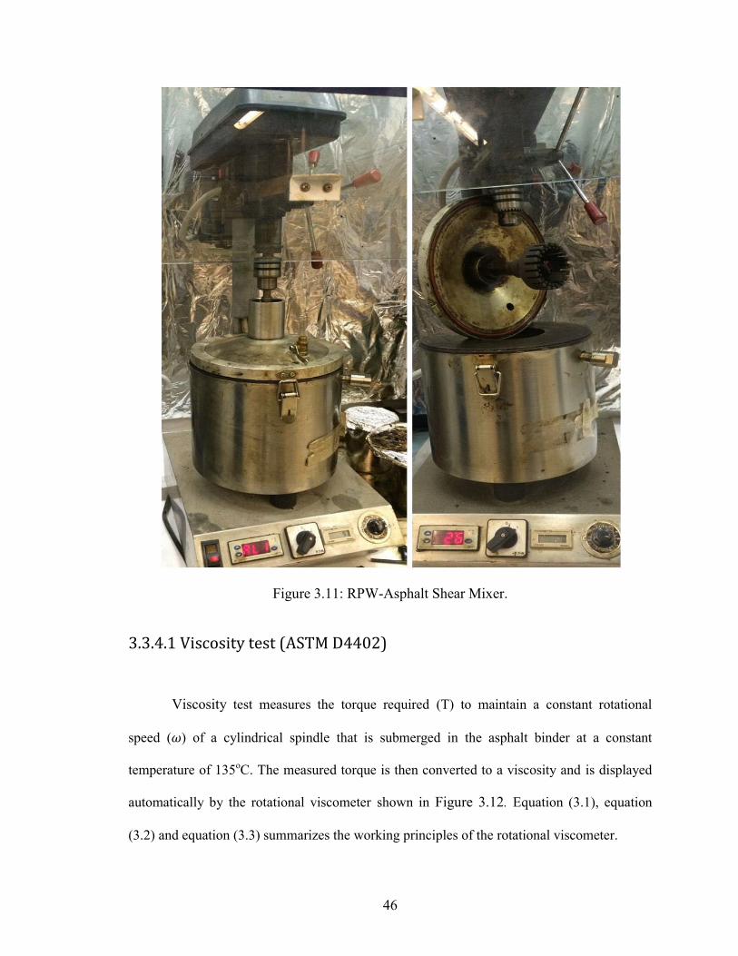
46
Figure 3.11: RPW-Asphalt Shear Mixer.
3.3.4.1 Viscosity test (ASTM D4402)
Viscosity test measures the torque required (T) to maintain a constant rotational
speed ( ) of a cylindrical spindle that is submerged in the asphalt binder at a constant
temperature of 135oC. The measured torque is then converted to a viscosity and is displayed
automatically by the rotational viscometer shown in Figure 3.12. Equation (3.1), equation
(3.2) and equation (3.3) summarizes the working principles of the rotational viscometer.
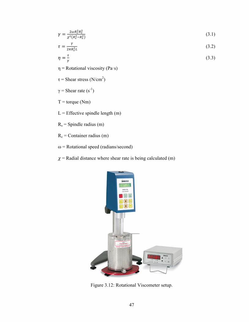
47
(3.1)
(3.2)
(3.3)
η = Rotational viscosity (Pa·s)
τ = Shear stress (N/cm2)
γ = Shear rate (s-1)
T = torque (Nm)
L = Effective spindle length (m)
Rs = Spindle radius (m)
Rc = Container radius (m)
ω = Rotational speed (radians/second)
= Radial distance where shear rate is being calculated (m)
Figure 3.12: Rotational Viscometer setup.
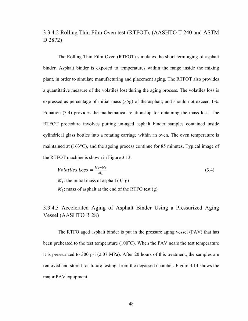
48
3.3.4.2 Rolling Thin Film Oven test (RTFOT), (AASHTO T 240 and ASTM D 2872)
The Rolling Thin-Film Oven (RTFOT) simulates the short term aging of asphalt
binder. Asphalt binder is exposed to temperatures within the range inside the mixing
plant, in order to simulate manufacturing and placement aging. The RTFOT also provides
a quantitative measure of the volatiles lost during the aging process. The volatiles loss is
expressed as percentage of initial mass (35g) of the asphalt, and should not exceed 1%.
Equation (3.4) provides the mathematical relationship for obtaining the mass loss. The
RTFOT procedure involves putting un-aged asphalt binder samples contained inside
cylindrical glass bottles into a rotating carriage within an oven. The oven temperature is
maintained at (163°C), and the ageing process continue for 85 minutes. Typical image of
the RTFOT machine is shown in Figure 3.13.
(3.4)
: the initial mass of asphalt (35 g)
: mass of asphalt at the end of the RTFO test (g)
3.3.4.3 Accelerated Aging of Asphalt Binder Using a Pressurized Aging Vessel (AASHTO R 28)
The RTFO aged asphalt binder is put in the pressure aging vessel (PAV) that has
been preheated to the test temperature (100oC). When the PAV nears the test temperature
it is pressurized to 300 psi (2.07 MPa). After 20 hours of this treatment, the samples are
removed and stored for future testing, from the degassed chamber. Figure 3.14 shows the
major PAV equipment
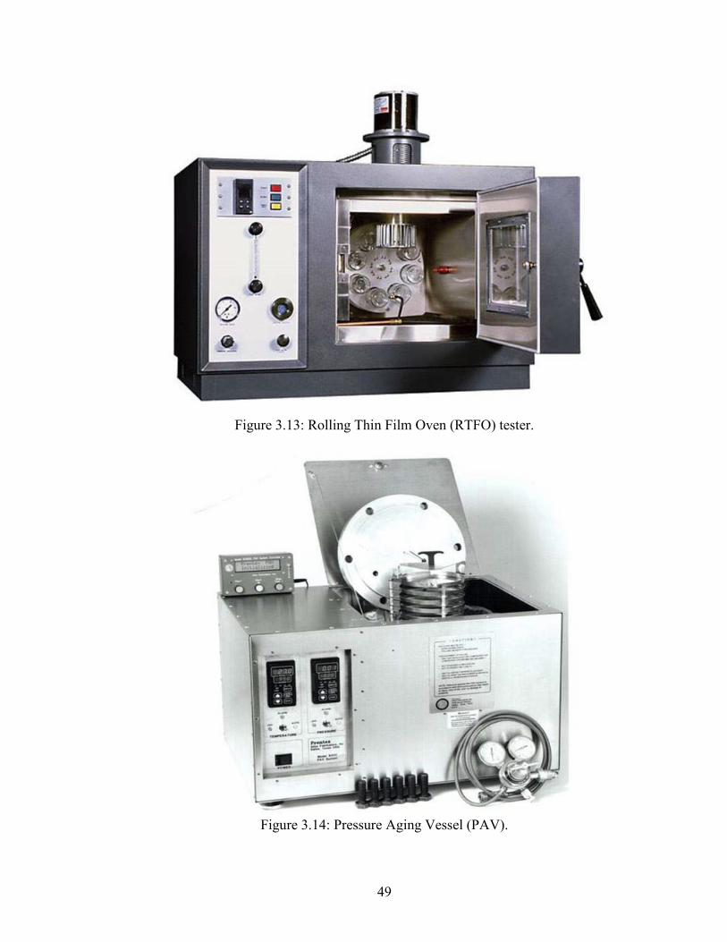
49
Figure 3.13: Rolling Thin Film Oven (RTFO) tester.
Figure 3.14: Pressure Aging Vessel (PAV).
50
3.3.4.4 Dynamic Shear Rheometer test (DSR), (AASHTO T 315)
Dynamic shear rheometer test is used to characterize the elastic and viscous
behavior of an asphalt binder. Equation (3.5) up to equation (3.9) describes the stress-
strain viscoelastic behavior of asphalt. The test is used in the Super-pave asphalt binder
PG specification. DSR test uses thin asphalt binder sample sandwiched in-between two
parallel circular plates. The upper plate oscillates across the sample at 10 rad/sec (1.59
Hz) creating a shearing action, while the lower plate is fixed. Equation (3.10), (3.11) and
(3.14) presents the mathematical relationship between the applied toque 'T', maximum
stress and strain with the complex modulus for DSR test setup. The rutting parameter
' ' must be maximized for minimal dissipated energy per load cycle at high
temperature. Likewise, the viscous component of the complex modulus ' ' has to
be minimized to eliminate fatigue cracking. Figure 3.15 shows a typical DSR machine.
(3.5)
(3.6)
(3.7)
(3.8)
(3.9)
(3.10)
(3.11)

51
(3.12)
(3.13)
: Complex shear modulus
: maximum applied strain
: sinusoidal strain function
: angular frequency (rad/s)
: time (s)
: maximum applied stress
: sinusoidal stress function
: the phase angle, or the lag between applied strain and stress
: storage or elastic modulus
: loss or viscous modulus
T : maximum applied torque
r : specimen radius (either 4 or 12.5 mm)
θ : deflection (rotation) angle (rad)
h : specimen height (1 or 2 mm)
: Dissipated energy per load cycle
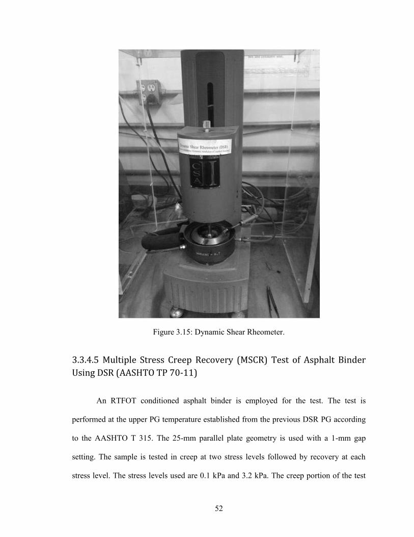
52
Figure 3.15: Dynamic Shear Rheometer.
3.3.4.5 Multiple Stress Creep Recovery (MSCR) Test of Asphalt Binder
Using DSR (AASHTO TP 70-11)
An RTFOT conditioned asphalt binder is employed for the test. The test is
performed at the upper PG temperature established from the previous DSR PG according
to the AASHTO T 315. The 25-mm parallel plate geometry is used with a 1-mm gap
setting. The sample is tested in creep at two stress levels followed by recovery at each
stress level. The stress levels used are 0.1 kPa and 3.2 kPa. The creep portion of the test
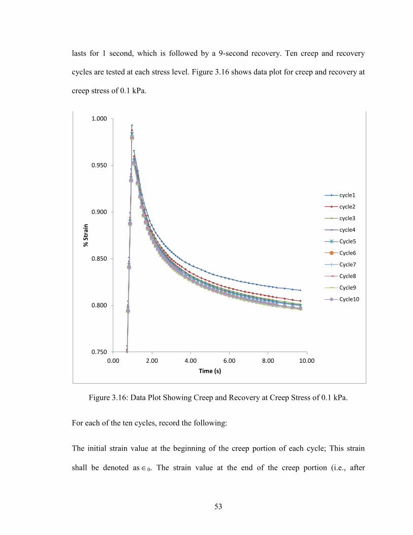
53
lasts for 1 second, which is followed by a 9-second recovery. Ten creep and recovery
cycles are tested at each stress level. Figure 3.16 shows data plot for creep and recovery at
creep stress of 0.1 kPa.
Figure 3.16: Data Plot Showing Creep and Recovery at Creep Stress of 0.1 kPa.
For each of the ten cycles, record the following:
The initial strain value at the beginning of the creep portion of each cycle; This strain
shall be denoted as 0. The strain value at the end of the creep portion (i.e., after
0.750
0.800
0.850
0.900
0.950
1.000
0.00 2.00 4.00 6.00 8.00 10.00
% S
trai
n
Time (s)
cycle1
cycle2
cycle3
cycle4
Cycle5
Cycle6
Cycle7
Cycle8
Cycle9
Cycle10

54
1.0 second) of each cycle; This strain shall be denoted as c. The adjusted strain value at
the end of the creep portion (i.e., after 1.0 second) of each cycle (1), which is calculated
as follows:
1 = c – 0 (3.14)
The strain value at the end of the recovery portion (i.e., after 10.0 second) of each cycle;
This strain shall be denoted as r. The adjusted strain value at the end of the recovery
portion (i.e., after 10.0 seconds) of each cycle (10), which is calculated as follows:
10 = r – 0 (3.15)
For each of the ten cycles, calculate the following at the creep stress level of 0.1 kPa:
Percent recovery r(0.1, N) for N = 1 to 10:
1 10
1
1000.1,r N
(3.16)
For each of the ten cycles, calculate the following at the creep stress level of 3.2 kPa:
Percent recovery r(3.2, N) for N = 1 to 10:
1 10
1
1003.2,r N
(3.17)
The average percent recovery at 0.1 kPa:
0.1
0.1,
10rSUM N
R
for N = 1 to 10 (3.18)
The average percent recovery at 3.2 kPa:

55
3.2
3.2,
10rSUM N
R
for N = 1 to 10 . (3.19)
The percent difference in recovery between 0.1 kPa and 3.2 kPa:
0.1 3.2
0.1
100diff
R RR
R
(3.20)
For each of the ten cycles at a creep stress of 0.1 kPa, calculate the non-recoverable creep
compliance, Jnr(0.1, N), kPa–1, as strain/stress:
100.1,0.1nrJ N
(3.21)
For each of the ten cycles at a creep stress of 3.2 kPa, calculate the non-recoverable creep
compliance, Jnr(3.2, N), kPa–1, as strain/stress:
103.2,3.2nrJ N
(3.22)
The average non-recoverable creep compliance at 0.1 kPa, 0.1nrJ , kPa–1:
0.1
0.1,
10nr
nrSUM J N
J
for N = 1 to 10 (3.23)
The average non-recoverable creep compliance at 3.2 kPa, 3.2nrJ , kPa–1:
3.2
3.2,
10nr
nrSUM J N
J
for N = 1 to 10 (3.24)
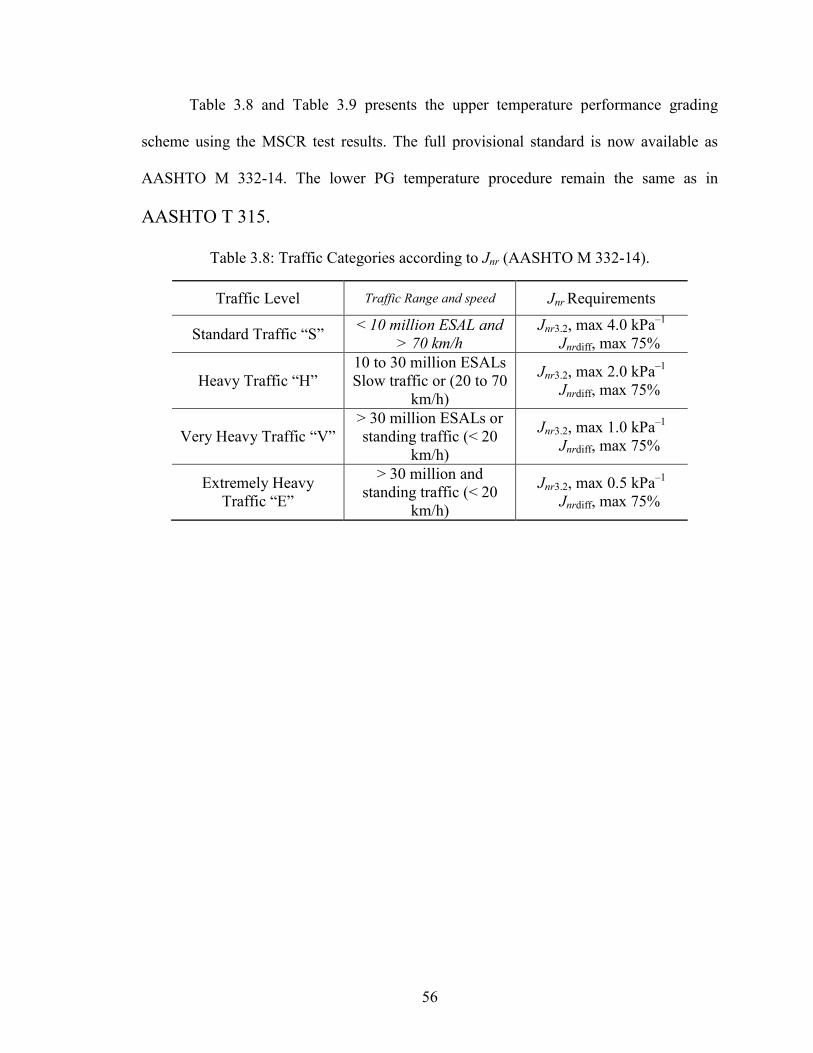
56
Table 3.8 and Table 3.9 presents the upper temperature performance grading
scheme using the MSCR test results. The full provisional standard is now available as
AASHTO M 332-14. The lower PG temperature procedure remain the same as in
AASHTO T 315.
Table 3.8: Traffic Categories according to Jnr (AASHTO M 332-14).
Traffic Level Traffic Range and speed Jnr Requirements
Standard Traffic “S” < 10 million ESAL and > 70 km/h
Jnr3.2, max 4.0 kPa–1
Jnrdiff, max 75%
Heavy Traffic “H” 10 to 30 million ESALs Slow traffic or (20 to 70
km/h)
Jnr3.2, max 2.0 kPa–1
Jnrdiff, max 75%
Very Heavy Traffic “V” > 30 million ESALs or standing traffic (< 20
km/h)
Jnr3.2, max 1.0 kPa–1
Jnrdiff, max 75%
Extremely Heavy Traffic “E”
> 30 million and standing traffic (< 20
km/h)
Jnr3.2, max 0.5 kPa–1
Jnrdiff, max 75%
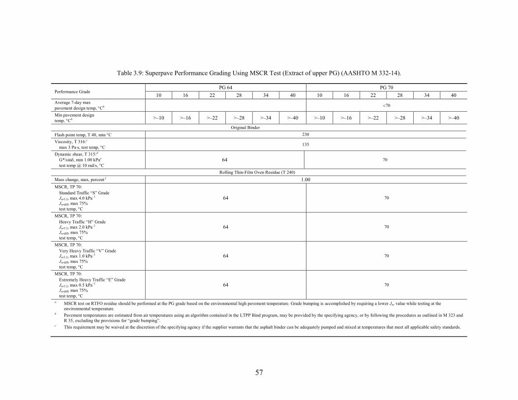
57
Table 3.9: Superpave Performance Grading Using MSCR Test (Extract of upper PG) (AASHTO M 332-14).
Performance Grade PG 64 PG 70
10 16 22 28 34 40 10 16 22 28 34 40 Average 7-day max pavement design temp, Cb
70
Min pavement design temp, Cb >–10 >–16 >–22 >–28 >–34 >–40 >–10 >–16 >–22 >–28 >–34 >–40
Original Binder Flash point temp, T 48, min C 230 Viscosity, T 316:c max 3 Pas, test temp, C 135
Dynamic shear, T 315:d G*/sin, min 1.00 kPae test temp @ 10 rad/s, C
64 70
Rolling Thin-Film Oven Residue (T 240) Mass change, max, percent f 1.00 MSCR, TP 70: Standard Traffic “S” Grade Jnr3.2, max 4.0 kPa–1
Jnrdiff, max 75% test temp, C
64 70
MSCR, TP 70: Heavy Traffic “H” Grade Jnr3.2, max 2.0 kPa–1
Jnrdiff, max 75% test temp, C
64 70
MSCR, TP 70: Very Heavy Traffic “V” Grade Jnr3.2, max 1.0 kPa–1
Jnrdiff, max 75% test temp, C
64 70
MSCR, TP 70: Extremely Heavy Traffic “E” Grade Jnr3.2, max 0.5 kPa–1
Jnrdiff, max 75% test temp, C
64 70
a MSCR test on RTFO residue should be performed at the PG grade based on the environmental high pavement temperature. Grade bumping is accomplished by requiring a lower Jnr value while testing at the environmental temperature.
b Pavement temperatures are estimated from air temperatures using an algorithm contained in the LTPP Bind program, may be provided by the specifying agency, or by following the procedures as outlined in M 323 and R 35, excluding the provisions for “grade bumping”.
c This requirement may be waived at the discretion of the specifying agency if the supplier warrants that the asphalt binder can be adequately pumped and mixed at temperatures that meet all applicable safety standards.
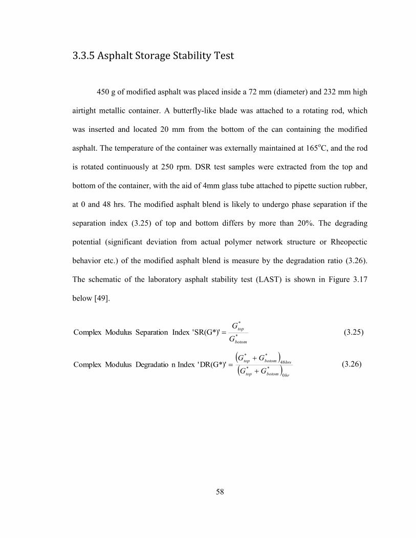
58
3.3.5 Asphalt Storage Stability Test
450 g of modified asphalt was placed inside a 72 mm (diameter) and 232 mm high
airtight metallic container. A butterfly-like blade was attached to a rotating rod, which
was inserted and located 20 mm from the bottom of the can containing the modified
asphalt. The temperature of the container was externally maintained at 165oC, and the rod
is rotated continuously at 250 rpm. DSR test samples were extracted from the top and
bottom of the container, with the aid of 4mm glass tube attached to pipette suction rubber,
at 0 and 48 hrs. The modified asphalt blend is likely to undergo phase separation if the
separation index (3.25) of top and bottom differs by more than 20%. The degrading
potential (significant deviation from actual polymer network structure or Rheopectic
behavior etc.) of the modified asphalt blend is measure by the degradation ratio (3.26).
The schematic of the laboratory asphalt stability test (LAST) is shown in Figure 3.17
below [49].
*
*
SR(G*)''Index Separation ModulusComplex botom
top
GG
(3.25)
hrbotomtop
hrsbotomtop
GG
GG
0**
48**
DR(G*)''Index n Degradatio ModulusComplex
(3.26)
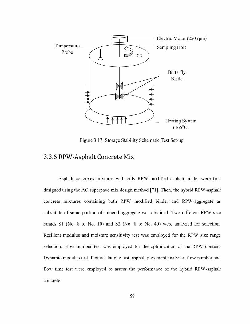
59
Figure 3.17: Storage Stability Schematic Test Set-up.
3.3.6 RPW-Asphalt Concrete Mix
Asphalt concretes mixtures with only RPW modified asphalt binder were first
designed using the AC superpave mix design method [71]. Then, the hybrid RPW-asphalt
concrete mixtures containing both RPW modified binder and RPW-aggregate as
substitute of some portion of mineral-aggregate was obtained. Two different RPW size
ranges S1 (No. 8 to No. 10) and S2 (No. 8 to No. 40) were analyzed for selection.
Resilient modulus and moisture sensitivity test was employed for the RPW size range
selection. Flow number test was employed for the optimization of the RPW content.
Dynamic modulus test, flexural fatigue test, asphalt pavement analyzer, flow number and
flow time test were employed to assess the performance of the hybrid RPW-asphalt
concrete.
Electric Motor (250 rpm)
Sampling Hole Temperature Probe
Butterfly Blade
Heating System (165oC)
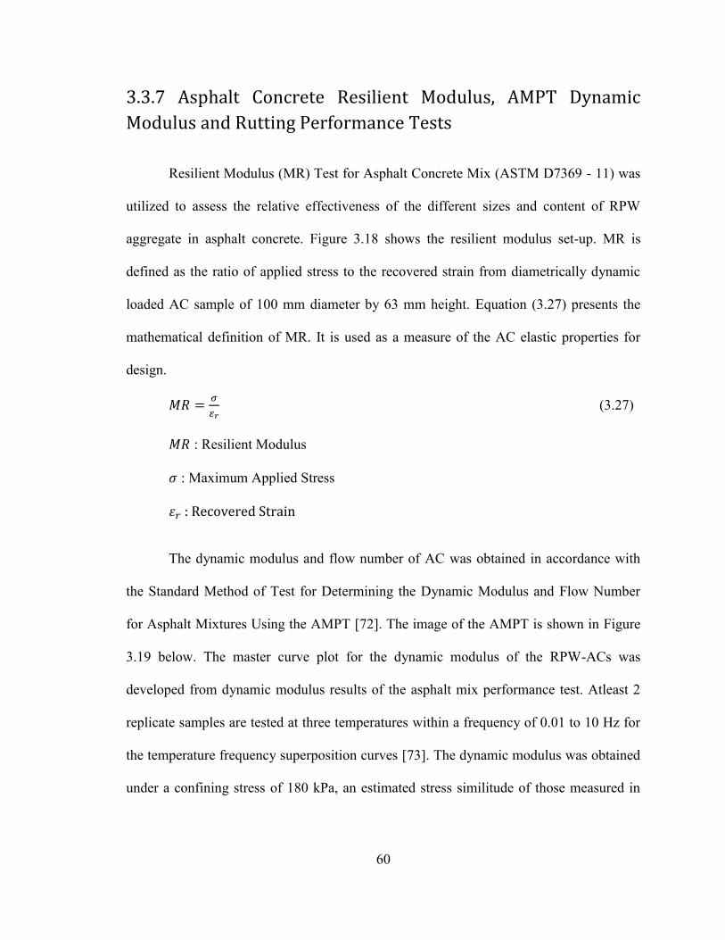
60
3.3.7 Asphalt Concrete Resilient Modulus, AMPT Dynamic
Modulus and Rutting Performance Tests
Resilient Modulus (MR) Test for Asphalt Concrete Mix (ASTM D7369 - 11) was
utilized to assess the relative effectiveness of the different sizes and content of RPW
aggregate in asphalt concrete. Figure 3.18 shows the resilient modulus set-up. MR is
defined as the ratio of applied stress to the recovered strain from diametrically dynamic
loaded AC sample of 100 mm diameter by 63 mm height. Equation (3.27) presents the
mathematical definition of MR. It is used as a measure of the AC elastic properties for
design.
(3.27)
: Resilient Modulus
: Maximum Applied Stress
: Recovered Strain
The dynamic modulus and flow number of AC was obtained in accordance with
the Standard Method of Test for Determining the Dynamic Modulus and Flow Number
for Asphalt Mixtures Using the AMPT [72]. The image of the AMPT is shown in Figure
3.19 below. The master curve plot for the dynamic modulus of the RPW-ACs was
developed from dynamic modulus results of the asphalt mix performance test. Atleast 2
replicate samples are tested at three temperatures within a frequency of 0.01 to 10 Hz for
the temperature frequency superposition curves [73]. The dynamic modulus was obtained
under a confining stress of 180 kPa, an estimated stress similitude of those measured in
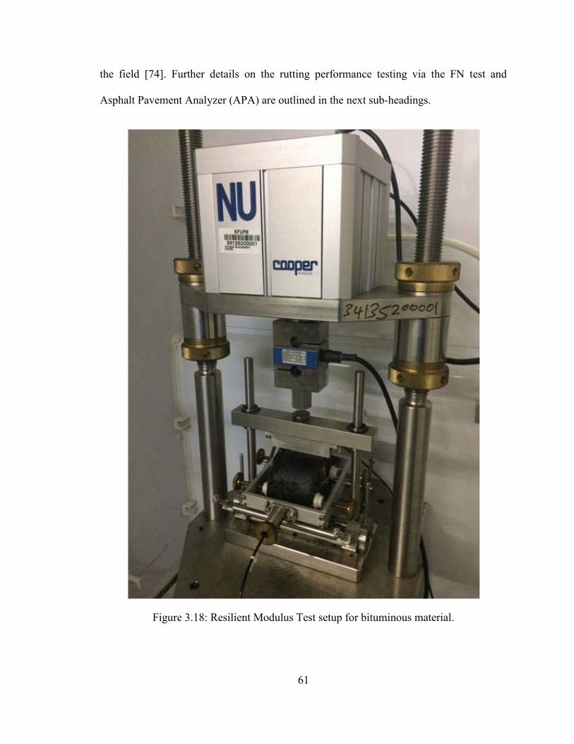
61
the field [74]. Further details on the rutting performance testing via the FN test and
Asphalt Pavement Analyzer (APA) are outlined in the next sub-headings.
Figure 3.18: Resilient Modulus Test setup for bituminous material.
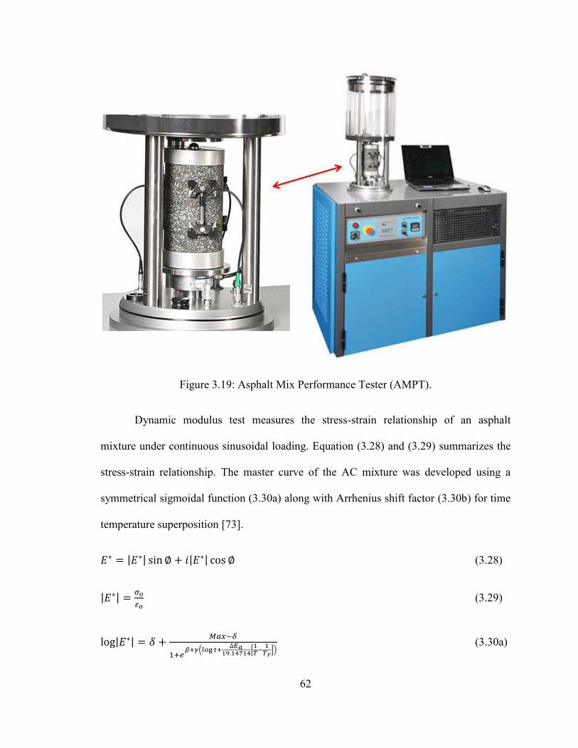
62
Figure 3.19: Asphalt Mix Performance Tester (AMPT).
Dynamic modulus test measures the stress-strain relationship of an asphalt
mixture under continuous sinusoidal loading. Equation (3.28) and (3.29) summarizes the
stress-strain relationship. The master curve of the AC mixture was developed using a
symmetrical sigmoidal function (3.30a) along with Arrhenius shift factor (3.30b) for time
temperature superposition [73].
(3.28)
(3.29)
(3.30a)
63
(3.30b)
(3.31)
(3.32)
Where:
: Complex Modulus
: Shift Factor
: Factor for limiting maximum dynamic modulus estimation
: Phase angle
: Maximum applied stress
: Peak of recoverable axial strain
: Dynamic Modulus
: Limiting Maximum Mixture Dynamic Modulus
: Void in Mineral Aggregate
: Void Filled with Asphalt
: Temperature
: Reference Temperature (oK)
: Limiting Maximum Modulus
: Loading Time
: Fitting Parameter
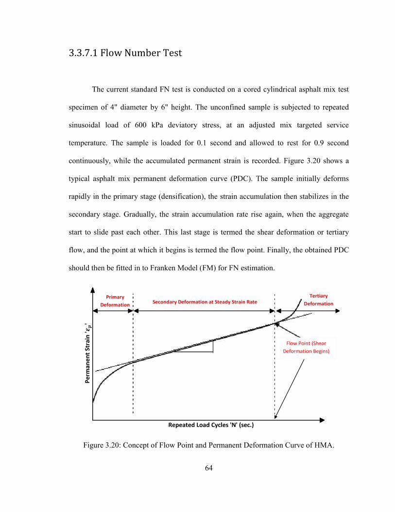
64
3.3.7.1 Flow Number Test
The current standard FN test is conducted on a cored cylindrical asphalt mix test
specimen of 4" diameter by 6" height. The unconfined sample is subjected to repeated
sinusoidal load of 600 kPa deviatory stress, at an adjusted mix targeted service
temperature. The sample is loaded for 0.1 second and allowed to rest for 0.9 second
continuously, while the accumulated permanent strain is recorded. Figure 3.20 shows a
typical asphalt mix permanent deformation curve (PDC). The sample initially deforms
rapidly in the primary stage (densification), the strain accumulation then stabilizes in the
secondary stage. Gradually, the strain accumulation rate rise again, when the aggregate
start to slide past each other. This last stage is termed the shear deformation or tertiary
flow, and the point at which it begins is termed the flow point. Finally, the obtained PDC
should then be fitted in to Franken Model (FM) for FN estimation.
Figure 3.20: Concept of Flow Point and Permanent Deformation Curve of HMA.
Primary
Deformation Secondary Deformation at Steady Strain Rate
Tertiary
Deformation
Flow Point (Shear
Deformation Begins)
P
erm
anen
t St
rain
'𝜺𝒑
'
Repeated Load Cycles 'N' (sec.)
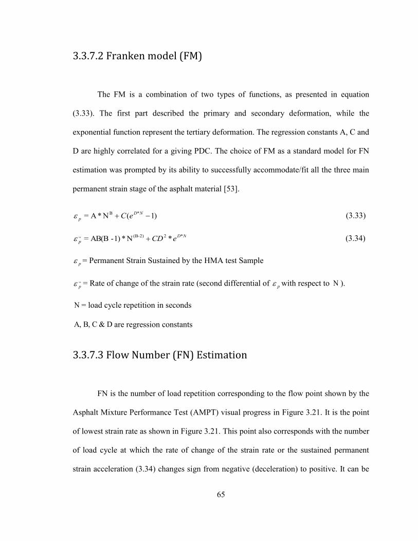
65
3.3.7.2 Franken model (FM)
The FM is a combination of two types of functions, as presented in equation
(3.33). The first part described the primary and secondary deformation, while the
exponential function represent the tertiary deformation. The regression constants A, C and
D are highly correlated for a giving PDC. The choice of FM as a standard model for FN
estimation was prompted by its ability to successfully accommodate/fit all the three main
permanent strain stage of the asphalt material [53].
)1(N*A= *B
NDp eC (3.33)
NDp eCD *22)-(B,, *N*1)-AB(B= (3.34)
p = Permanent Strain Sustained by the HMA test Sample
,,p = Rate of change of the strain rate (second differential of p with respect to N ).
N = load cycle repetition in seconds
D & C B, A, are regression constants
3.3.7.3 Flow Number (FN) Estimation
FN is the number of load repetition corresponding to the flow point shown by the
Asphalt Mixture Performance Test (AMPT) visual progress in Figure 3.21. It is the point
of lowest strain rate as shown in Figure 3.21. This point also corresponds with the number
of load cycle at which the rate of change of the strain rate or the sustained permanent
strain acceleration (3.34) changes sign from negative (deceleration) to positive. It can be
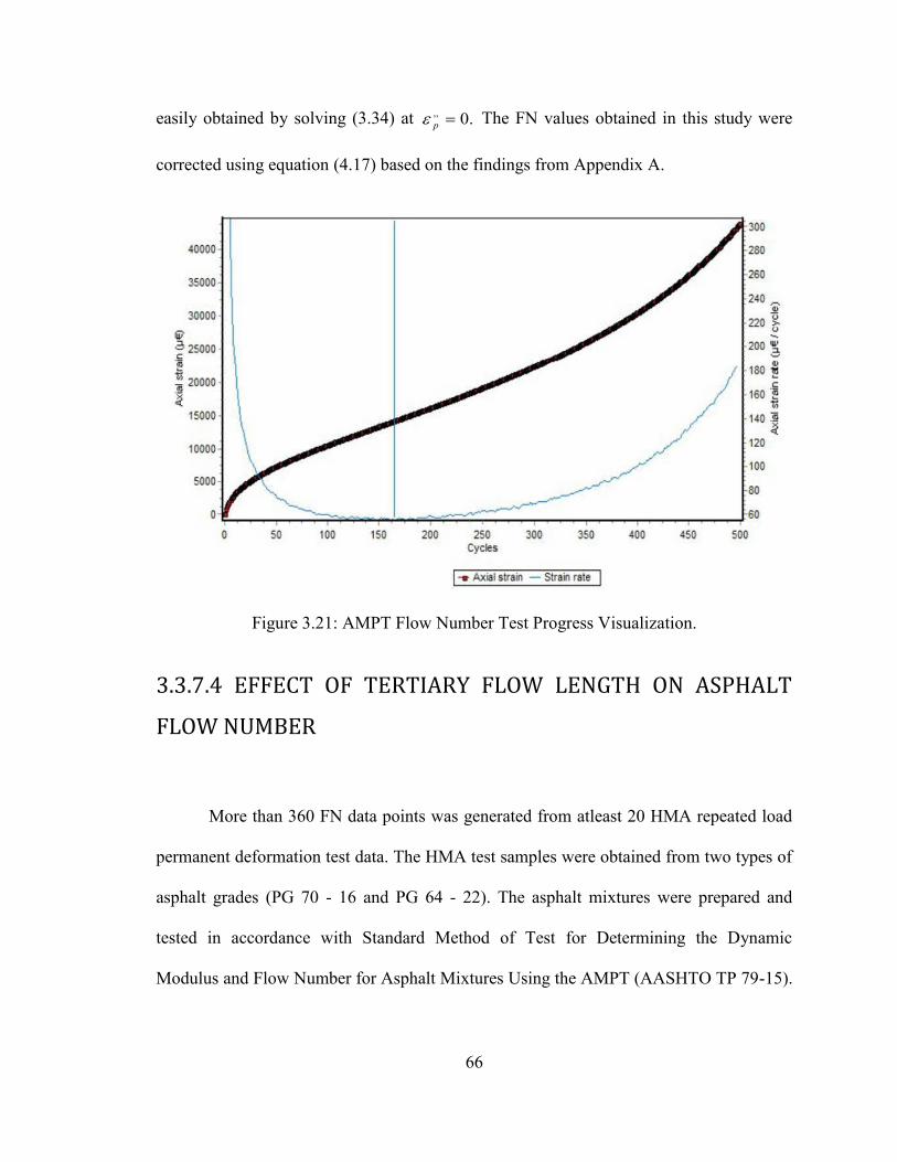
66
easily obtained by solving (3.34) at .0,,p The FN values obtained in this study were
corrected using equation (4.17) based on the findings from Appendix A.
Figure 3.21: AMPT Flow Number Test Progress Visualization.
3.3.7.4 EFFECT OF TERTIARY FLOW LENGTH ON ASPHALT
FLOW NUMBER
More than 360 FN data points was generated from atleast 20 HMA repeated load
permanent deformation test data. The HMA test samples were obtained from two types of
asphalt grades (PG 70 - 16 and PG 64 - 22). The asphalt mixtures were prepared and
tested in accordance with Standard Method of Test for Determining the Dynamic
Modulus and Flow Number for Asphalt Mixtures Using the AMPT (AASHTO TP 79-15).
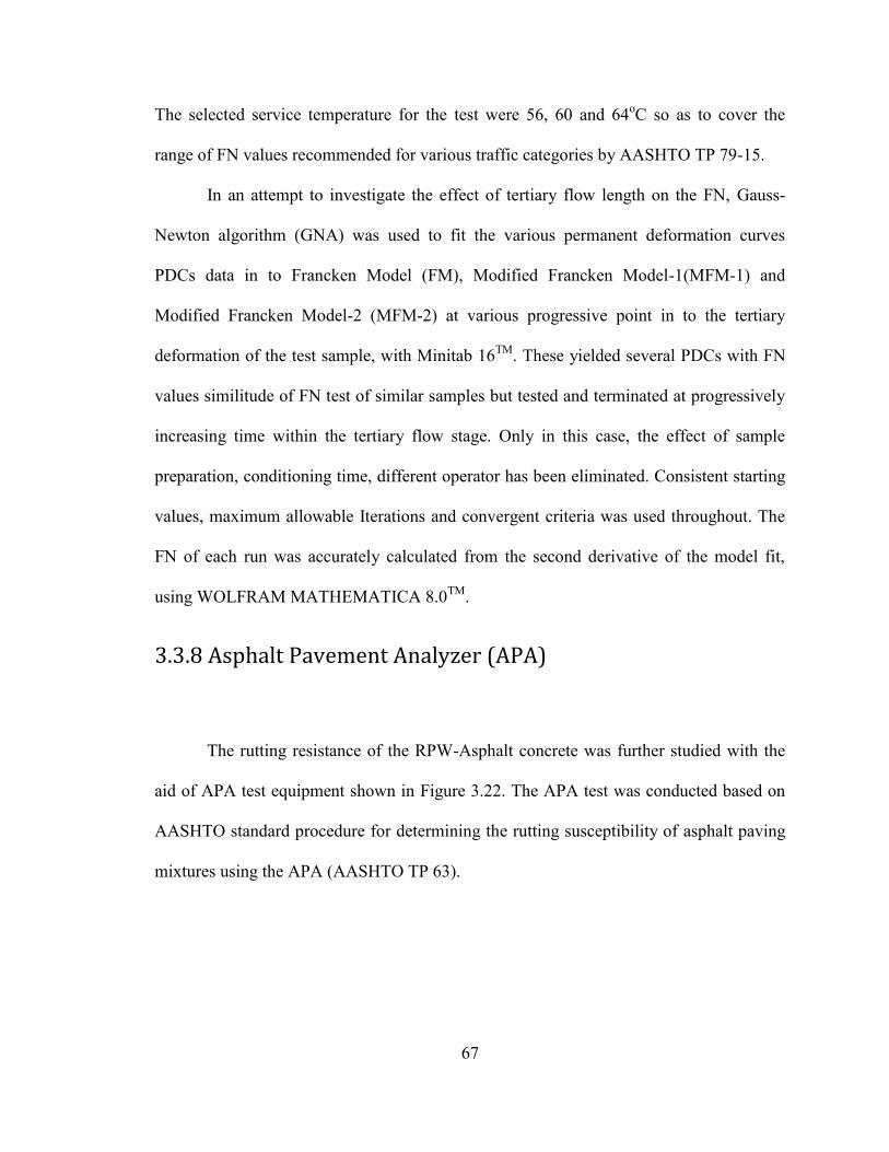
67
The selected service temperature for the test were 56, 60 and 64oC so as to cover the
range of FN values recommended for various traffic categories by AASHTO TP 79-15.
In an attempt to investigate the effect of tertiary flow length on the FN, Gauss-
Newton algorithm (GNA) was used to fit the various permanent deformation curves
PDCs data in to Francken Model (FM), Modified Francken Model-1(MFM-1) and
Modified Francken Model-2 (MFM-2) at various progressive point in to the tertiary
deformation of the test sample, with Minitab 16TM. These yielded several PDCs with FN
values similitude of FN test of similar samples but tested and terminated at progressively
increasing time within the tertiary flow stage. Only in this case, the effect of sample
preparation, conditioning time, different operator has been eliminated. Consistent starting
values, maximum allowable Iterations and convergent criteria was used throughout. The
FN of each run was accurately calculated from the second derivative of the model fit,
using WOLFRAM MATHEMATICA 8.0TM.
3.3.8 Asphalt Pavement Analyzer (APA)
The rutting resistance of the RPW-Asphalt concrete was further studied with the
aid of APA test equipment shown in Figure 3.22. The APA test was conducted based on
AASHTO standard procedure for determining the rutting susceptibility of asphalt paving
mixtures using the APA (AASHTO TP 63).
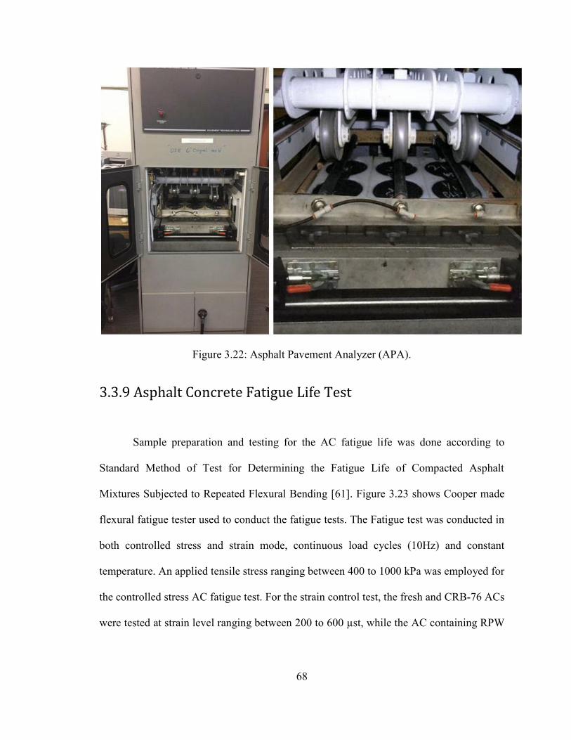
68
Figure 3.22: Asphalt Pavement Analyzer (APA).
3.3.9 Asphalt Concrete Fatigue Life Test
Sample preparation and testing for the AC fatigue life was done according to
Standard Method of Test for Determining the Fatigue Life of Compacted Asphalt
Mixtures Subjected to Repeated Flexural Bending [61]. Figure 3.23 shows Cooper made
flexural fatigue tester used to conduct the fatigue tests. The Fatigue test was conducted in
both controlled stress and strain mode, continuous load cycles (10Hz) and constant
temperature. An applied tensile stress ranging between 400 to 1000 kPa was employed for
the controlled stress AC fatigue test. For the strain control test, the fresh and CRB-76 ACs
were tested at strain level ranging between 200 to 600 µst, while the AC containing RPW

69
as aggregate substitute are tested at higher strain ranging from 350 to 1000 µst due to
their high flexural resilience.
(3.35)
(3.36)
(3.37)
(3.38)
Where:
: maximum tensile stress
: space between inside clamps
P : applied load
S : Stiffness
b : average beam width
h : average beam height
: maximum tensile strain
δ : measured deformation
L : beam length between outside clamps
φ : phase angle (degrees)
f : load frequency (Hz)
s : time lag between maximum load and deflection
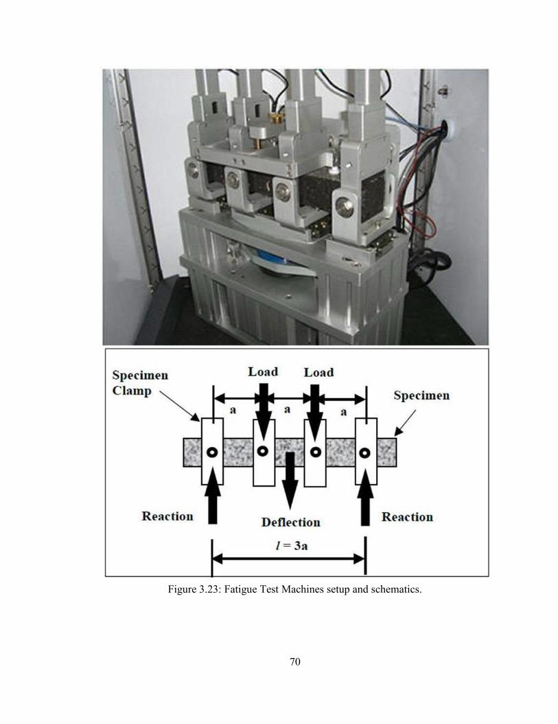
70
Figure 3.23: Fatigue Test Machines setup and schematics.
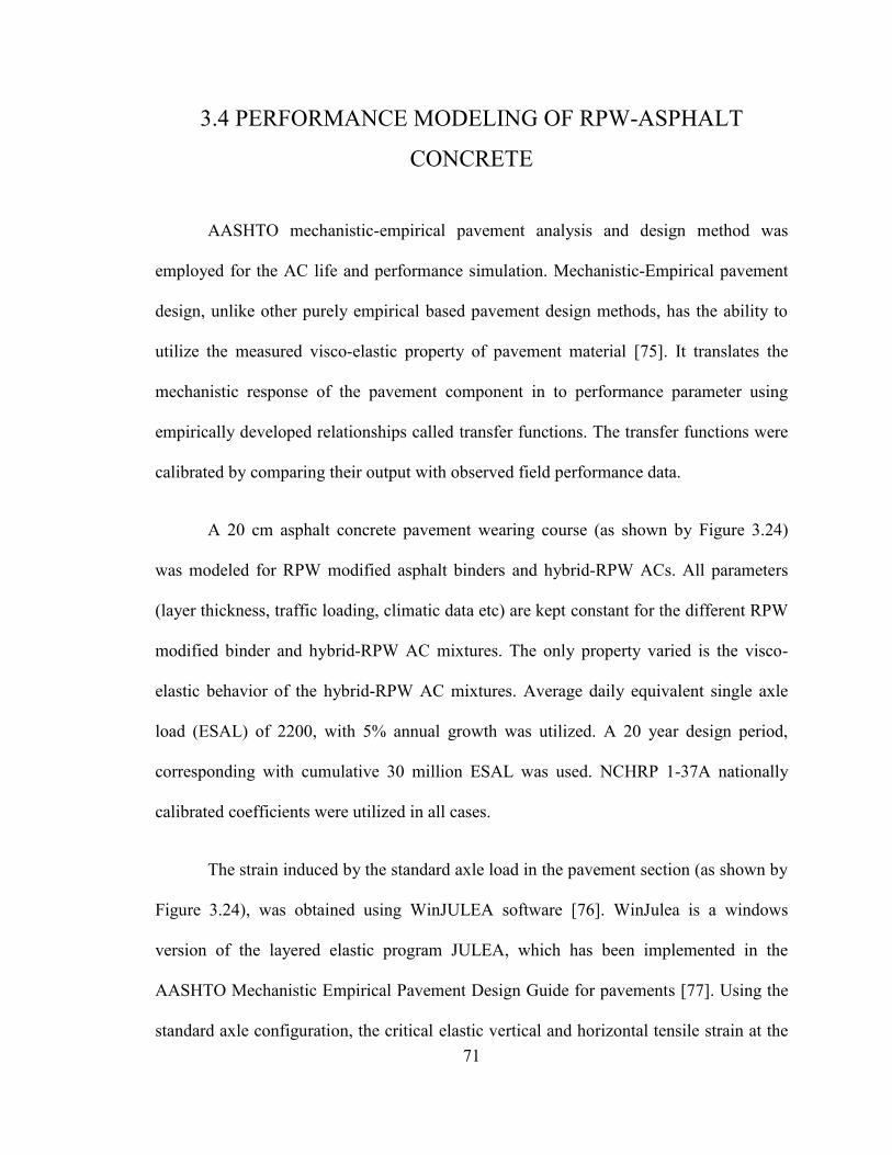
71
3.4 PERFORMANCE MODELING OF RPW-ASPHALT
CONCRETE
AASHTO mechanistic-empirical pavement analysis and design method was
employed for the AC life and performance simulation. Mechanistic-Empirical pavement
design, unlike other purely empirical based pavement design methods, has the ability to
utilize the measured visco-elastic property of pavement material [75]. It translates the
mechanistic response of the pavement component in to performance parameter using
empirically developed relationships called transfer functions. The transfer functions were
calibrated by comparing their output with observed field performance data.
A 20 cm asphalt concrete pavement wearing course (as shown by Figure 3.24)
was modeled for RPW modified asphalt binders and hybrid-RPW ACs. All parameters
(layer thickness, traffic loading, climatic data etc) are kept constant for the different RPW
modified binder and hybrid-RPW AC mixtures. The only property varied is the visco-
elastic behavior of the hybrid-RPW AC mixtures. Average daily equivalent single axle
load (ESAL) of 2200, with 5% annual growth was utilized. A 20 year design period,
corresponding with cumulative 30 million ESAL was used. NCHRP 1-37A nationally
calibrated coefficients were utilized in all cases.
The strain induced by the standard axle load in the pavement section (as shown by
Figure 3.24), was obtained using WinJULEA software [76]. WinJulea is a windows
version of the layered elastic program JULEA, which has been implemented in the
AASHTO Mechanistic Empirical Pavement Design Guide for pavements [77]. Using the
standard axle configuration, the critical elastic vertical and horizontal tensile strain at the
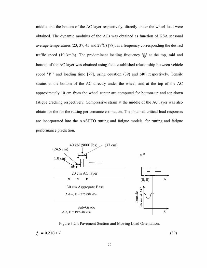
72
middle and the bottom of the AC layer respectively, directly under the wheel load were
obtained. The dynamic modulus of the ACs was obtained as function of KSA seasonal
average temperatures (23, 37, 45 and 27oC) [78], at a frequency corresponding the desired
traffic speed (10 km/h). The predominant loading frequency ' ' at the top, mid and
bottom of the AC layer was obtained using field established relationship between vehicle
speed ' ' and loading time [79], using equation (39) and (40) respectively. Tensile
strains at the bottom of the AC directly under the wheel, and at the top of the AC
approximately 10 cm from the wheel center are computed for bottom-up and top-down
fatigue cracking respectively. Compressive strain at the middle of the AC layer was also
obtain for the for the rutting performance estimation. The obtained critical load responses
are incorporated into the AASHTO rutting and fatigue models, for rutting and fatigue
performance prediction.
Figure 3.24: Pavement Section and Moving Load Orientation.
(39)
40 kN (9000 lbs) (24.5 cm)
(37 cm)
(0, 0)
y
x
Tens
ile
Stra
in a
t AC
bo
ttom
x
20 cm AC layer
30 cm Aggregate Base
Sub-Grade
A-1-a, E = 275790 kPa
A-3, E = 199948 kPa
(10 cm)
73
(40)
3.4.1 AC Rutting Performance Model and Transfer Function
Equation (3.41) represents the generalized AC rutting performance model [77].
Where is the accumulated vertical permanent deformation (mm/mm); : vertically
imposed resilient strain on laboratory test sample to obtain (mm/mm); is the number
of cumulative load repetition; : Layer temperature (oC), depth below the
surface, thickness of AC layer and depth confinement factor respectively.
(3.41)
(3.42)
(3.43)
(3.44)
are regression constants.
3.4.3 AC Fatigue Performance Model and Transfer Function
Equation (3.45) shows the general fatigue performance model employed for the fatigue
performance estimation [77]. Where is the number of load repetition to cracking, is
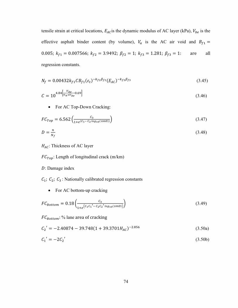
74
tensile strain at critical locations, is the dynamic modulus of AC layer (kPa), is the
effective asphalt binder content (by volume), is the AC air void and
: are all
regression constants.
(3.45)
(3.46)
For AC Top-Down Cracking:
(3.47)
(3.48)
: Thickness of AC layer
: Length of longitudinal crack (m/km)
: Damage index
: Nationally calibrated regression constants
For AC bottom-up cracking
(3.49)
: % lane area of cracking
(3.50a)
(3.50b)
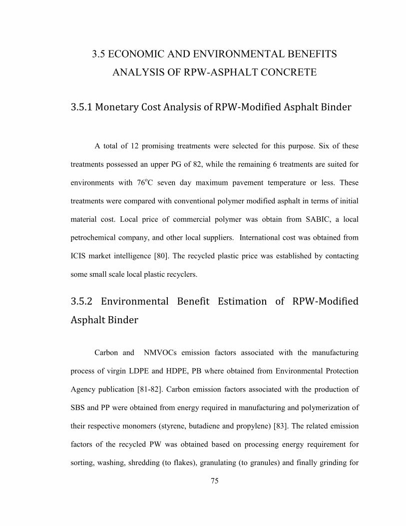
75
3.5 ECONOMIC AND ENVIRONMENTAL BENEFITS
ANALYSIS OF RPW-ASPHALT CONCRETE
3.5.1 Monetary Cost Analysis of RPW-Modified Asphalt Binder
A total of 12 promising treatments were selected for this purpose. Six of these
treatments possessed an upper PG of 82, while the remaining 6 treatments are suited for
environments with 76oC seven day maximum pavement temperature or less. These
treatments were compared with conventional polymer modified asphalt in terms of initial
material cost. Local price of commercial polymer was obtain from SABIC, a local
petrochemical company, and other local suppliers. International cost was obtained from
ICIS market intelligence [80]. The recycled plastic price was established by contacting
some small scale local plastic recyclers.
3.5.2 Environmental Benefit Estimation of RPW-Modified
Asphalt Binder
Carbon and NMVOCs emission factors associated with the manufacturing
process of virgin LDPE and HDPE, PB where obtained from Environmental Protection
Agency publication [81-82]. Carbon emission factors associated with the production of
SBS and PP were obtained from energy required in manufacturing and polymerization of
their respective monomers (styrene, butadiene and propylene) [83]. The related emission
factors of the recycled PW was obtained based on processing energy requirement for
sorting, washing, shredding (to flakes), granulating (to granules) and finally grinding for
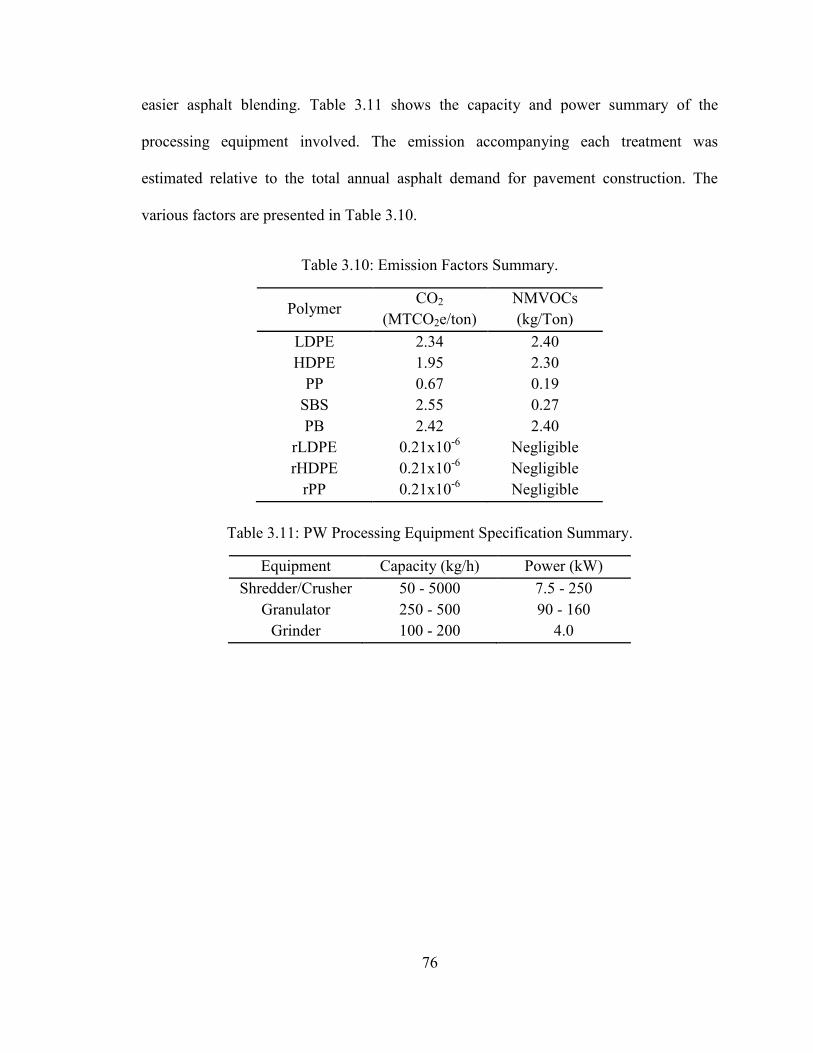
76
easier asphalt blending. Table 3.11 shows the capacity and power summary of the
processing equipment involved. The emission accompanying each treatment was
estimated relative to the total annual asphalt demand for pavement construction. The
various factors are presented in Table 3.10.
Table 3.10: Emission Factors Summary.
Polymer CO2
(MTCO2e/ton) NMVOCs (kg/Ton)
LDPE 2.34 2.40 HDPE 1.95 2.30
PP 0.67 0.19 SBS 2.55 0.27 PB 2.42 2.40
rLDPE 0.21x10⁻⁶ Negligible rHDPE 0.21x10⁻⁶ Negligible
rPP 0.21x10⁻⁶ Negligible
Table 3.11: PW Processing Equipment Specification Summary.
Equipment Capacity (kg/h) Power (kW) Shredder/Crusher 50 - 5000 7.5 - 250
Granulator 250 - 500 90 - 160 Grinder 100 - 200 4.0
77
Summary: The methodology followed in carrying out the various tasks
involved in this research has been described. The study has been divided into three
phases. The first phase addresses the identification of RPWs that can be used in asphalt
modification or replacement of aggregate, followed by the evaluation of RPW-modified
asphalts. Different potential RPWs will be screened and selected based on thermal and
rheological techniques. The second phase involves analyses of the performance and
mechanical properties of RPW-modified AC mixtures composed of both pure binder and
pure RWP or blended modified asphalt binder. The third phase includes data analyses and
reporting. The overall work sequence and content has been summarized in the work flow
chart a shown Figure 3.1. The RPW modified asphalt test experimental design was
presented. The RPW-AC mix optimization and performance evaluation guide was also
explained. The detail description of the test and analysis methods employed was provided
in the last subheadings. Details of AC mechanic-empirical performance modeling method
adopted was also described.
78
CHAPTER 4
RESULTS AND DISCUSSION
Introduction: This chapter presents detail result discussion of all the tasks in this
study. Sections covered include the RPW screening process, RPW asphalt binder
blending optimization, performance grading of the RPW asphalt binder and storage
stability analysis of the RPW asphalt binder. The superpave mix design of the RPW
asphalt concrete, content and size range optimization of the hybrid RPW AC, and finally
the results of effect of tertiary deformation length on the FN was also discussed. Each
main subheading discusses an independent phase of this research.
4.1 RPW SCREENING RESULTS
The summary of the RPW screening is presented in Table 4.1. DSC analysis
(ASTM E1356), Using DSC Q 1000 model yielded the melting point of the obtained
RPW. The RPWs with melting point below 200oC were selected as potential asphalt
binder modifiers. 200oC was considered the limit, since asphalt-polymer blending above
this temperature for prolong duration results in excessive oxidation. Since aggregate are
not required to fully integrate with the asphalt binder, all of the RPW are eligible for AC
modification through aggregate substitution. The RPW-asphalt blending temperatures
were obtained by adding approximately 45oC to their corresponding melting points. This
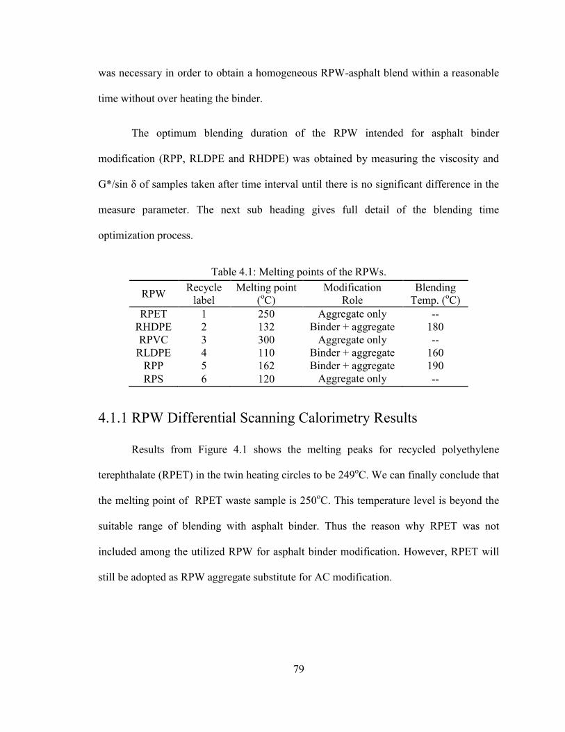
79
was necessary in order to obtain a homogeneous RPW-asphalt blend within a reasonable
time without over heating the binder.
The optimum blending duration of the RPW intended for asphalt binder
modification (RPP, RLDPE and RHDPE) was obtained by measuring the viscosity and
G*/sin δ of samples taken after time interval until there is no significant difference in the
measure parameter. The next sub heading gives full detail of the blending time
optimization process.
Table 4.1: Melting points of the RPWs.
RPW Recycle label
Melting point (oC)
Modification Role
Blending Temp. (oC)
RPET 1 250 Aggregate only -- RHDPE 2 132 Binder + aggregate 180 RPVC 3 300 Aggregate only --
RLDPE 4 110 Binder + aggregate 160 RPP 5 162 Binder + aggregate 190 RPS 6 120 Aggregate only --
4.1.1 RPW Differential Scanning Calorimetry Results
Results from Figure 4.1 shows the melting peaks for recycled polyethylene
terephthalate (RPET) in the twin heating circles to be 249oC. We can finally conclude that
the melting point of RPET waste sample is 250oC. This temperature level is beyond the
suitable range of blending with asphalt binder. Thus the reason why RPET was not
included among the utilized RPW for asphalt binder modification. However, RPET will
still be adopted as RPW aggregate substitute for AC modification.
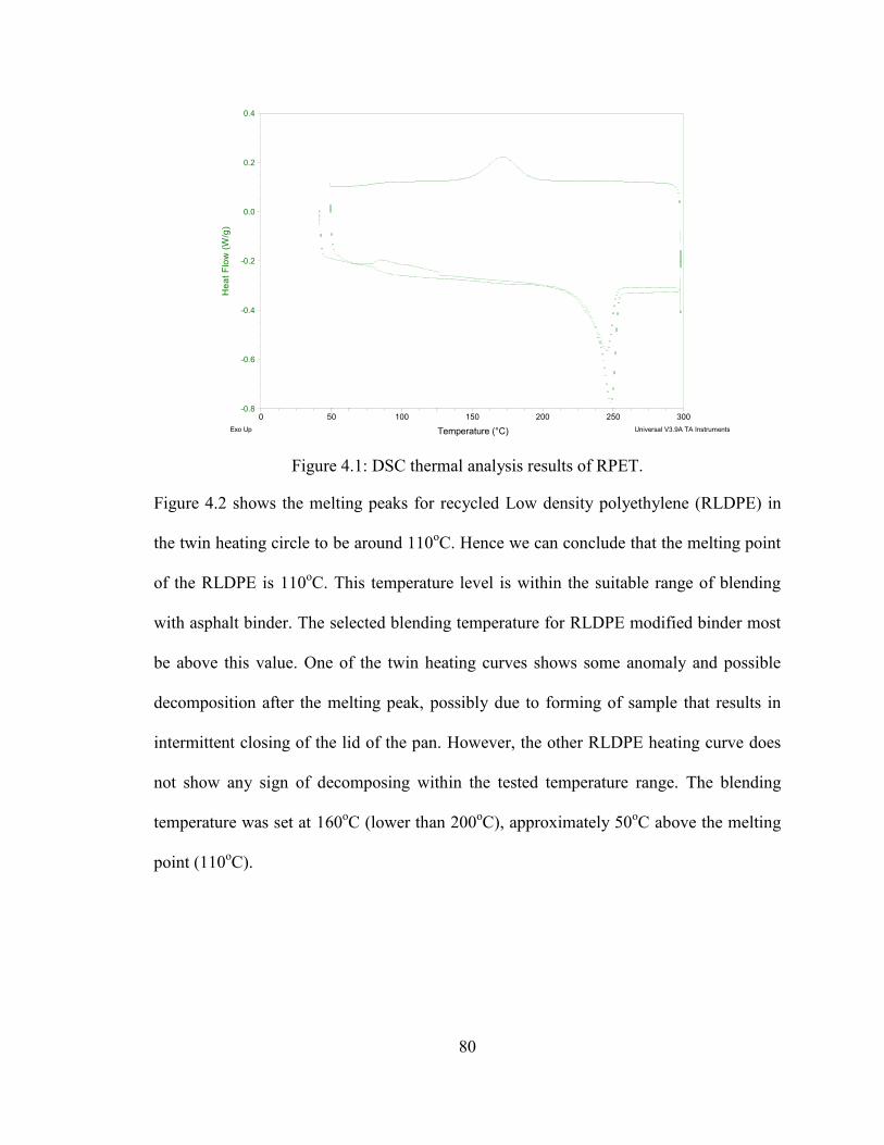
80
Figure 4.1: DSC thermal analysis results of RPET.
Figure 4.2 shows the melting peaks for recycled Low density polyethylene (RLDPE) in
the twin heating circle to be around 110oC. Hence we can conclude that the melting point
of the RLDPE is 110oC. This temperature level is within the suitable range of blending
with asphalt binder. The selected blending temperature for RLDPE modified binder most
be above this value. One of the twin heating curves shows some anomaly and possible
decomposition after the melting peak, possibly due to forming of sample that results in
intermittent closing of the lid of the pan. However, the other RLDPE heating curve does
not show any sign of decomposing within the tested temperature range. The blending
temperature was set at 160oC (lower than 200oC), approximately 50oC above the melting
point (110oC).
-0.8
-0.6
-0.4
-0.2
0.0
0.2
0.4
Hea
t Flo
w (W
/g)
0 50 100 150 200 250 300
Temperature (°C)
Sample: CompositSize: 7.0640 mgMethod: Heat/Cool/Heat
DSCFile: C:...\DSC results of RPW\1.001Operator: MofizRun Date: 28-May-14 09:21Instrument: DSC Q1000 V9.4 Build 287
Exo Up Universal V3.9A TA Instruments
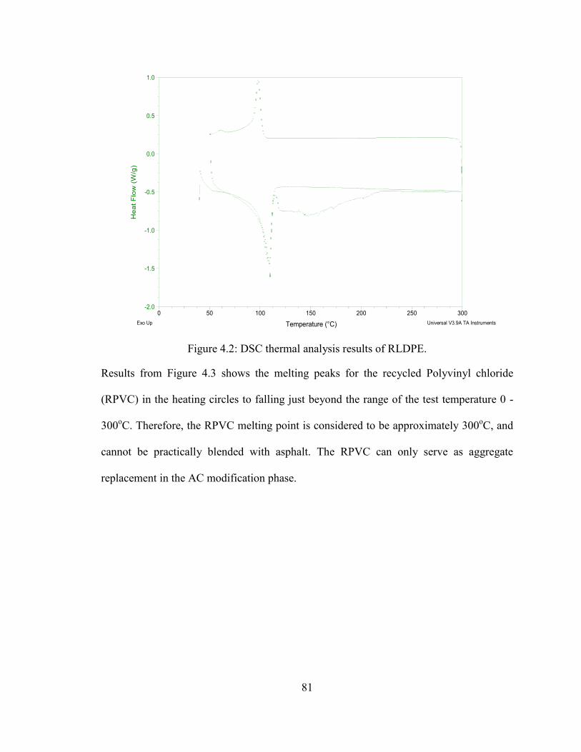
81
Figure 4.2: DSC thermal analysis results of RLDPE.
Results from Figure 4.3 shows the melting peaks for the recycled Polyvinyl chloride
(RPVC) in the heating circles to falling just beyond the range of the test temperature 0 -
300oC. Therefore, the RPVC melting point is considered to be approximately 300oC, and
cannot be practically blended with asphalt. The RPVC can only serve as aggregate
replacement in the AC modification phase.
-2.0
-1.5
-1.0
-0.5
0.0
0.5
1.0
Hea
t Flo
w (
W/g
)
0 50 100 150 200 250 300
Temperature (°C)
Sample: CompositSize: 5.8740 mgMethod: Heat/Cool/Heat
DSCFile: C:...\DSC results of RPW\2.001Operator: MofizRun Date: 01-Jun-14 10:46Instrument: DSC Q1000 V9.4 Build 287
Exo Up Universal V3.9A TA Instruments
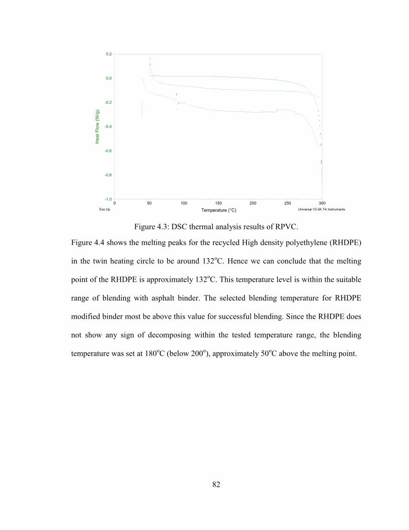
82
Figure 4.3: DSC thermal analysis results of RPVC.
Figure 4.4 shows the melting peaks for the recycled High density polyethylene (RHDPE)
in the twin heating circle to be around 132oC. Hence we can conclude that the melting
point of the RHDPE is approximately 132oC. This temperature level is within the suitable
range of blending with asphalt binder. The selected blending temperature for RHDPE
modified binder most be above this value for successful blending. Since the RHDPE does
not show any sign of decomposing within the tested temperature range, the blending
temperature was set at 180oC (below 200o), approximately 50oC above the melting point.
-1.0
-0.8
-0.6
-0.4
-0.2
0.0
0.2
Hea
t Flo
w (W
/g)
0 50 100 150 200 250 300
Temperature (°C)
Sample: CompositSize: 6.5320 mgMethod: Heat/Cool/Heat
DSCFile: C:...\DSC results of RPW\3.001Operator: MofizRun Date: 28-May-14 12:54Instrument: DSC Q1000 V9.4 Build 287
Exo Up Universal V3.9A TA Instruments
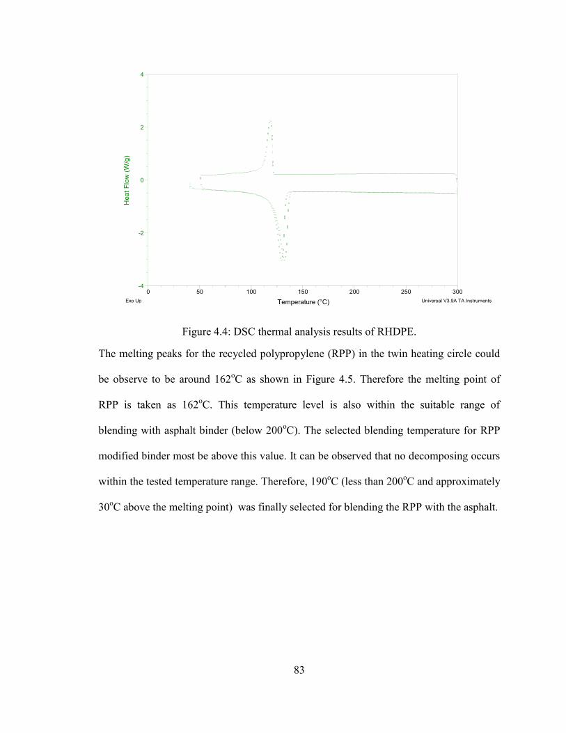
83
Figure 4.4: DSC thermal analysis results of RHDPE.
The melting peaks for the recycled polypropylene (RPP) in the twin heating circle could
be observe to be around 162oC as shown in Figure 4.5. Therefore the melting point of
RPP is taken as 162oC. This temperature level is also within the suitable range of
blending with asphalt binder (below 200oC). The selected blending temperature for RPP
modified binder most be above this value. It can be observed that no decomposing occurs
within the tested temperature range. Therefore, 190oC (less than 200oC and approximately
30oC above the melting point) was finally selected for blending the RPP with the asphalt.
-4
-2
0
2
4
Hea
t Flo
w (W
/g)
0 50 100 150 200 250 300
Temperature (°C)
Sample: CompositSize: 6.8160 mgMethod: Heat/Cool/Heat
DSCFile: C:...\DSC results of RPW\4.001Operator: MofizRun Date: 28-May-14 14:41Instrument: DSC Q1000 V9.4 Build 287
Exo Up Universal V3.9A TA Instruments
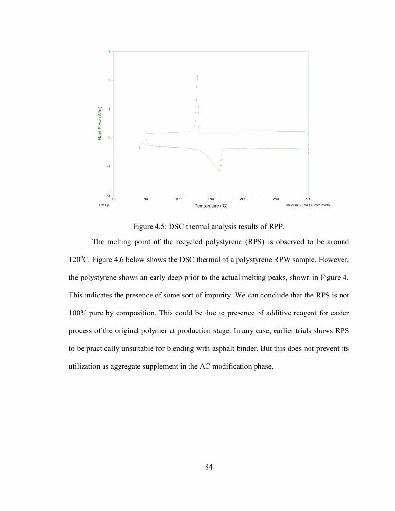
84
Figure 4.5: DSC thermal analysis results of RPP.
The melting point of the recycled polystyrene (RPS) is observed to be around
120oC. Figure 4.6 below shows the DSC thermal of a polystyrene RPW sample. However,
the polystyrene shows an early deep prior to the actual melting peaks, shown in Figure 4.
This indicates the presence of some sort of impurity. We can conclude that the RPS is not
100% pure by composition. This could be due to presence of additive reagent for easier
process of the original polymer at production stage. In any case, earlier trials shows RPS
to be practically unsuitable for blending with asphalt binder. But this does not prevent its
utilization as aggregate supplement in the AC modification phase.
-2
-1
0
1
2
3
Hea
t Flo
w (
W/g
)
0 50 100 150 200 250 300
Temperature (°C)
Sample: CompositSize: 5.7330 mgMethod: Heat/Cool/Heat
DSCFile: C:...\DSC results of RPW\5.003Operator: MofizRun Date: 01-Jun-14 12:32Instrument: DSC Q1000 V9.4 Build 287
Exo Up Universal V3.9A TA Instruments
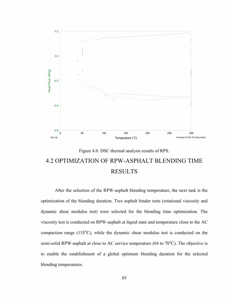
85
Figure 4.6: DSC thermal analysis results of RPS.
4.2 OPTIMIZATION OF RPW-ASPHALT BLENDING TIME
RESULTS
After the selection of the RPW-asphalt blending temperature, the next task is the
optimization of the blending duration. Two asphalt binder tests (rotational viscosity and
dynamic shear modulus test) were selected for the blending time optimization. The
viscosity test is conducted on RPW-asphalt at liquid state and temperature close to the AC
compaction range (135oC), while the dynamic shear modulus test is conducted on the
semi-solid RPW-asphalt at close to AC service temperature (64 to 70oC). The objective is
to enable the establishment of a global optimum blending duration for the selected
blending temperatures.
-0.6
-0.4
-0.2
0.0
0.2
Hea
t Flo
w (
W/g
)
0 50 100 150 200 250 300
Temperature (°C)
Sample: CompositSize: 6.7830 mgMethod: Heat/Cool/Heat
DSCFile: C:...\DSC results of RPW\6.001Operator: MofizRun Date: 01-Jun-14 08:59Instrument: DSC Q1000 V9.4 Build 287
Exo Up Universal V3.9A TA Instruments
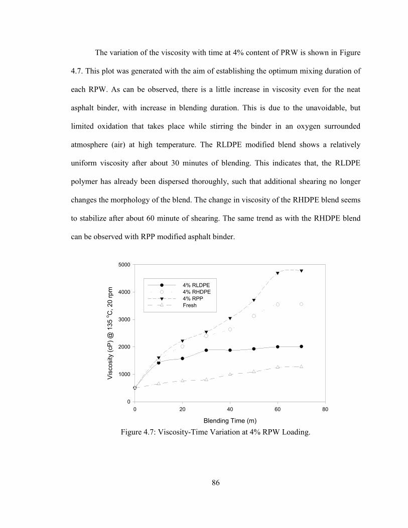
86
The variation of the viscosity with time at 4% content of PRW is shown in Figure
4.7. This plot was generated with the aim of establishing the optimum mixing duration of
each RPW. As can be observed, there is a little increase in viscosity even for the neat
asphalt binder, with increase in blending duration. This is due to the unavoidable, but
limited oxidation that takes place while stirring the binder in an oxygen surrounded
atmosphere (air) at high temperature. The RLDPE modified blend shows a relatively
uniform viscosity after about 30 minutes of blending. This indicates that, the RLDPE
polymer has already been dispersed thoroughly, such that additional shearing no longer
changes the morphology of the blend. The change in viscosity of the RHDPE blend seems
to stabilize after about 60 minute of shearing. The same trend as with the RHDPE blend
can be observed with RPP modified asphalt binder.
Figure 4.7: Viscosity-Time Variation at 4% RPW Loading.
Blending Time (m)
0 20 40 60 80
Vis
cosi
ty (c
P) @
135
o C, 2
0 rp
m
0
1000
2000
3000
4000
5000
4% RLDPE 4% RHDPE 4% RPP Fresh
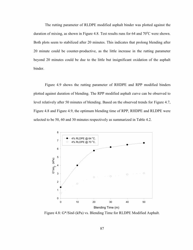
87
The rutting parameter of RLDPE modified asphalt binder was plotted against the
duration of mixing, as shown in Figure 4.8. Test results runs for 64 and 70oC were shown.
Both plots seem to stabilized after 20 minutes. This indicates that prolong blending after
20 minute could be counter-productive, as the little increase in the rutting parameter
beyond 20 minutes could be due to the little but insignificant oxidation of the asphalt
binder.
Figure 4.9 shows the rutting parameter of RHDPE and RPP modified binders
plotted against duration of blending. The RPP modified asphalt curve can be observed to
level relatively after 50 minutes of blending. Based on the observed trends for Figure 4.7,
Figure 4.8 and Figure 4.9, the optimum blending time of RPP, RHDPE and RLDPE were
selected to be 50, 60 and 30 minutes respectively as summarized in Table 4.2.
Figure 4.8: G*/Sinδ (kPa) vs. Blending Time for RLDPE Modified Asphalt.
Blending Time (m)
0 10 20 30 40 50
G*/s
in
(kPa
)
0
1
2
3
4
5
6
7
8
4% RLDPE @ 64 oC. 4% RLDPE @ 70 oC.
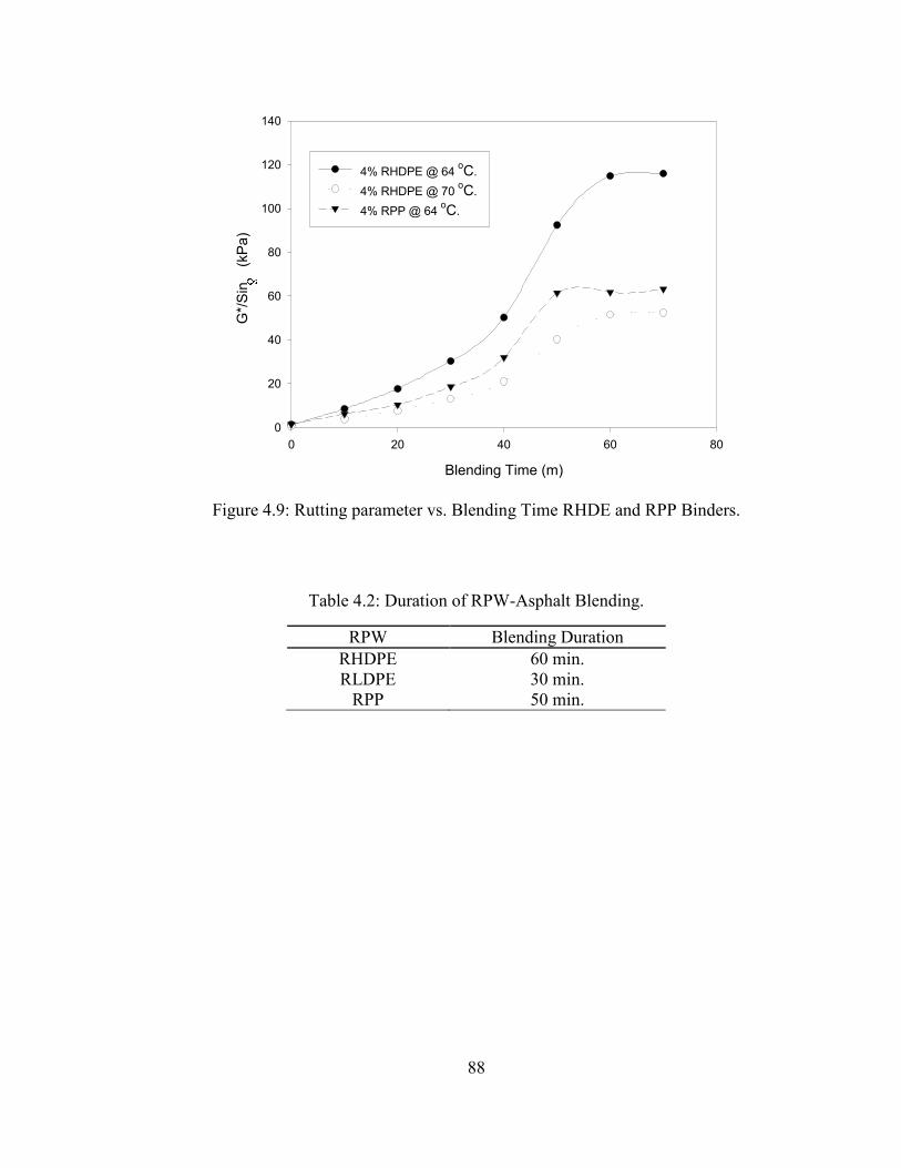
88
Figure 4.9: Rutting parameter vs. Blending Time RHDE and RPP Binders.
Table 4.2: Duration of RPW-Asphalt Blending.
RPW Blending Duration RHDPE 60 min. RLDPE 30 min.
RPP 50 min.
Blending Time (m)
0 20 40 60 80
G*/
Sin
(k
Pa)
0
20
40
60
80
100
120
140
4% RHDPE @ 64 oC. 4% RHDPE @ 70 oC. 4% RPP @ 64 oC.
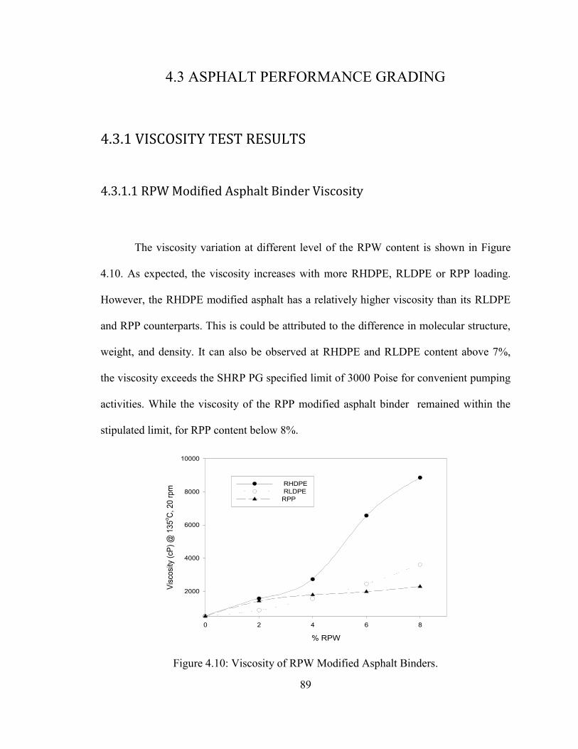
89
4.3 ASPHALT PERFORMANCE GRADING
4.3.1 VISCOSITY TEST RESULTS
4.3.1.1 RPW Modified Asphalt Binder Viscosity
The viscosity variation at different level of the RPW content is shown in Figure
4.10. As expected, the viscosity increases with more RHDPE, RLDPE or RPP loading.
However, the RHDPE modified asphalt has a relatively higher viscosity than its RLDPE
and RPP counterparts. This is could be attributed to the difference in molecular structure,
weight, and density. It can also be observed at RHDPE and RLDPE content above 7%,
the viscosity exceeds the SHRP PG specified limit of 3000 Poise for convenient pumping
activities. While the viscosity of the RPP modified asphalt binder remained within the
stipulated limit, for RPP content below 8%.
Figure 4.10: Viscosity of RPW Modified Asphalt Binders.
% RPW
0 2 4 6 8
Visc
osity
(cP)
@ 1
35o C,
20
rpm
2000
4000
6000
8000
10000
RHDPE RLDPE RPP

90
4.3.1.2 RLDPE + SBS Modified Asphalt Binders
The viscosity of a RLDPE-SBS binder appreciates with increase in either RLDPE
or SBS, as can be observed from Figure 4.11. This is confirmed from the trends exhibited
by blends containing either RLDPE or SBS alone. This increasing trend happened to be
maintained by blends containing both RLDPE and SBS polymer, due to the constructive
interaction between the RLDPE and SBS polymer micro-structural network. Their
individual micro-structural linkage reinforced each other, and continue to develop more
connections as either the RLDPE or SBS increases. This phenomena leads to an increased
inter-layer movement resistance, which in turn translate to a more viscous modified
binder. Most of the RLDPE-SBS blends meet the super-pave viscosity requirement limit.
However, blends containing more than 6% RLDPE in addition to SBS failed to pass the
viscosity criterion.
Figure 4.11: Viscosities of RLDPE-SBS modified binders.
% SBS
0.0 0.5 1.0 1.5 2.0 2.5
Vis
cosi
ty (c
P) a
t 135
o C, 2
0rpm
0
2000
4000
6000
8000
10000
0% RLDPE 2% RLDPE 4% RLDPE 6% RLDPE 8% RLDPE
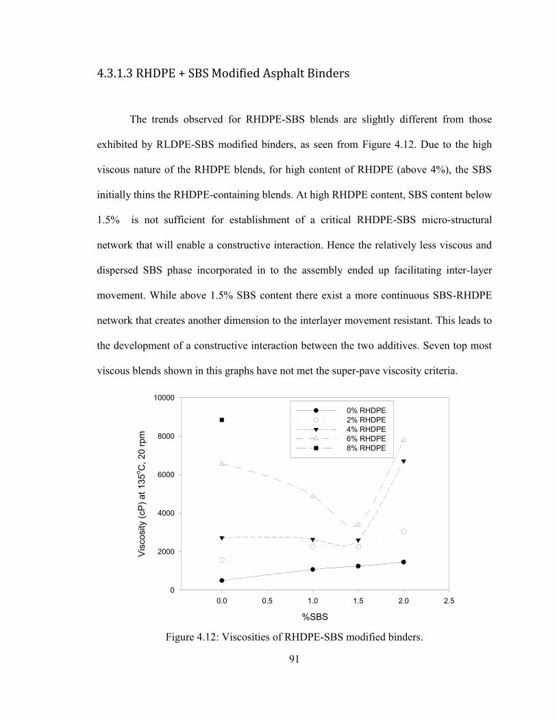
91
4.3.1.3 RHDPE + SBS Modified Asphalt Binders
The trends observed for RHDPE-SBS blends are slightly different from those
exhibited by RLDPE-SBS modified binders, as seen from Figure 4.12. Due to the high
viscous nature of the RHDPE blends, for high content of RHDPE (above 4%), the SBS
initially thins the RHDPE-containing blends. At high RHDPE content, SBS content below
1.5% is not sufficient for establishment of a critical RHDPE-SBS micro-structural
network that will enable a constructive interaction. Hence the relatively less viscous and
dispersed SBS phase incorporated in to the assembly ended up facilitating inter-layer
movement. While above 1.5% SBS content there exist a more continuous SBS-RHDPE
network that creates another dimension to the interlayer movement resistant. This leads to
the development of a constructive interaction between the two additives. Seven top most
viscous blends shown in this graphs have not met the super-pave viscosity criteria.
Figure 4.12: Viscosities of RHDPE-SBS modified binders.
%SBS
0.0 0.5 1.0 1.5 2.0 2.5
Vis
cosi
ty (c
P) a
t 135
o C, 2
0 rp
m
0
2000
4000
6000
8000
10000
0% RHDPE 2% RHDPE 4% RHDPE 6% RHDPE 8% RHDPE
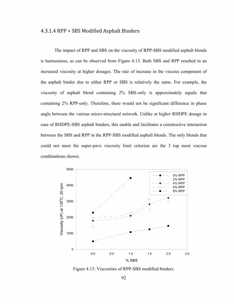
92
4.3.1.4 RPP + SBS Modified Asphalt Binders
The impact of RPP and SBS on the viscosity of RPP-SBS modified asphalt blends
is harmonious, as can be observed from Figure 4.13. Both SBS and RPP resulted in an
increased viscosity at higher dosages. The rate of increase in the viscous component of
the asphalt binder due to either RPP or SBS is relatively the same. For example, the
viscosity of asphalt blend containing 2% SBS-only is approximately equals that
containing 2% RPP-only. Therefore, there would not be significant difference in phase
angle between the various micro-structural network. Unlike at higher RHDPE dosage in
case of RHDPE-SBS asphalt binders, this enable and facilitates a constructive interaction
between the SBS and RPP in the RPP-SBS modified asphalt blends. The only blends that
could not meet the super-pave viscosity limit criterion are the 3 top most viscous
combinations shown.
Figure 4.13: Viscosities of RPP-SBS modified binders.
% SBS
0.0 0.5 1.0 1.5 2.0 2.5
Vis
cosi
ty (c
P) a
t 135
o C, 2
0 rp
m
0
1000
2000
3000
4000
5000
0% RPP 2% RPP 4% RPP 6% RPP 8% RPP
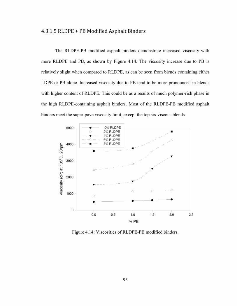
93
4.3.1.5 RLDPE + PB Modified Asphalt Binders
The RLDPE-PB modified asphalt binders demonstrate increased viscosity with
more RLDPE and PB, as shown by Figure 4.14. The viscosity increase due to PB is
relatively slight when compared to RLDPE, as can be seen from blends containing either
LDPE or PB alone. Increased viscosity due to PB tend to be more pronounced in blends
with higher content of RLDPE. This could be as a results of much polymer-rich phase in
the high RLDPE-containing asphalt binders. Most of the RLDPE-PB modified asphalt
binders meet the super-pave viscosity limit, except the top six viscous blends.
Figure 4.14: Viscosities of RLDPE-PB modified binders.
% PB
0.0 0.5 1.0 1.5 2.0 2.5
Vis
cosi
ty (c
P) a
t 135
o C, 2
0rpm
0
1000
2000
3000
4000
5000 0% RLDPE 2% RLDPE 4% RLDPE 6% RLDPE 8% RLDPE
94
4.3.1.6 RHDPE + PB Modified Asphalt Binders
The RHDPE-PB blended asphalt binders exhibit lower viscosities than their
RHDPE-only counter parts, as depicted in Figure 4.15. As can be observed, there is a
decreasing viscosity trend as the PB content increases. The rate of decrease in viscosity is
more rapid for asphalt blends containing higher RHDPE. Unlike the RLDPE blends, the
RHDPE blends exhibits a very high viscosity (as high as 9000 cP for 8% RHDPE
content). While on the other hand, PB can only results in a relatively slight viscosity
increment. So for up to 4% of RHDPE containing blends, the mild PB was only
successful in slightly lubricating RHDPE blends inter-layers. Hence resulting in reduced
inter-layer friction resistance. However, for blends containing higher RHDPE dosage that
have a continuous RHDPE micro-structural network. The resulting decrease in the
interlayer friction translate into higher loss in viscosity. Hence, the PB here served a vital
role that un-stiffen the viscous RHDPE modified asphalt binder. The topmost seven
viscous blends shown did not meet the super-pave viscosity limits. That is, those blends
containing more 4% RHDPE.
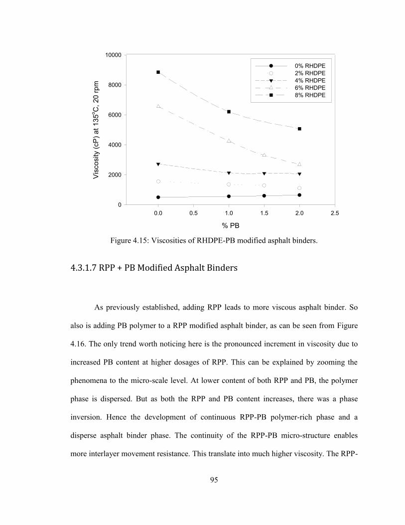
95
Figure 4.15: Viscosities of RHDPE-PB modified asphalt binders.
4.3.1.7 RPP + PB Modified Asphalt Binders
As previously established, adding RPP leads to more viscous asphalt binder. So
also is adding PB polymer to a RPP modified asphalt binder, as can be seen from Figure
4.16. The only trend worth noticing here is the pronounced increment in viscosity due to
increased PB content at higher dosages of RPP. This can be explained by zooming the
phenomena to the micro-scale level. At lower content of both RPP and PB, the polymer
phase is dispersed. But as both the RPP and PB content increases, there was a phase
inversion. Hence the development of continuous RPP-PB polymer-rich phase and a
disperse asphalt binder phase. The continuity of the RPP-PB micro-structure enables
more interlayer movement resistance. This translate into much higher viscosity. The RPP-
% PB
0.0 0.5 1.0 1.5 2.0 2.5
Vis
cosi
ty (c
P) a
t 135
o C, 2
0 rp
m
0
2000
4000
6000
8000
10000
0% RHDPE 2% RHDPE 4% RHDPE 6% RHDPE 8% RHDPE
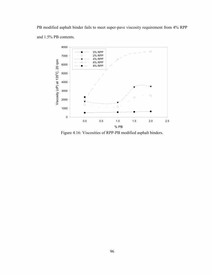
96
PB modified asphalt binder fails to meet super-pave viscosity requirement from 4% RPP
and 1.5% PB contents.
Figure 4.16: Viscosities of RPP-PB modified asphalt binders.
% PB
0.0 0.5 1.0 1.5 2.0 2.5
Vis
cosi
ty (c
P) a
t 135
o C, 2
0 rp
m
0
1000
2000
3000
4000
5000
6000
7000
8000
0% RPP 2% RPP 4% RPP 6% RPP 8% RPP
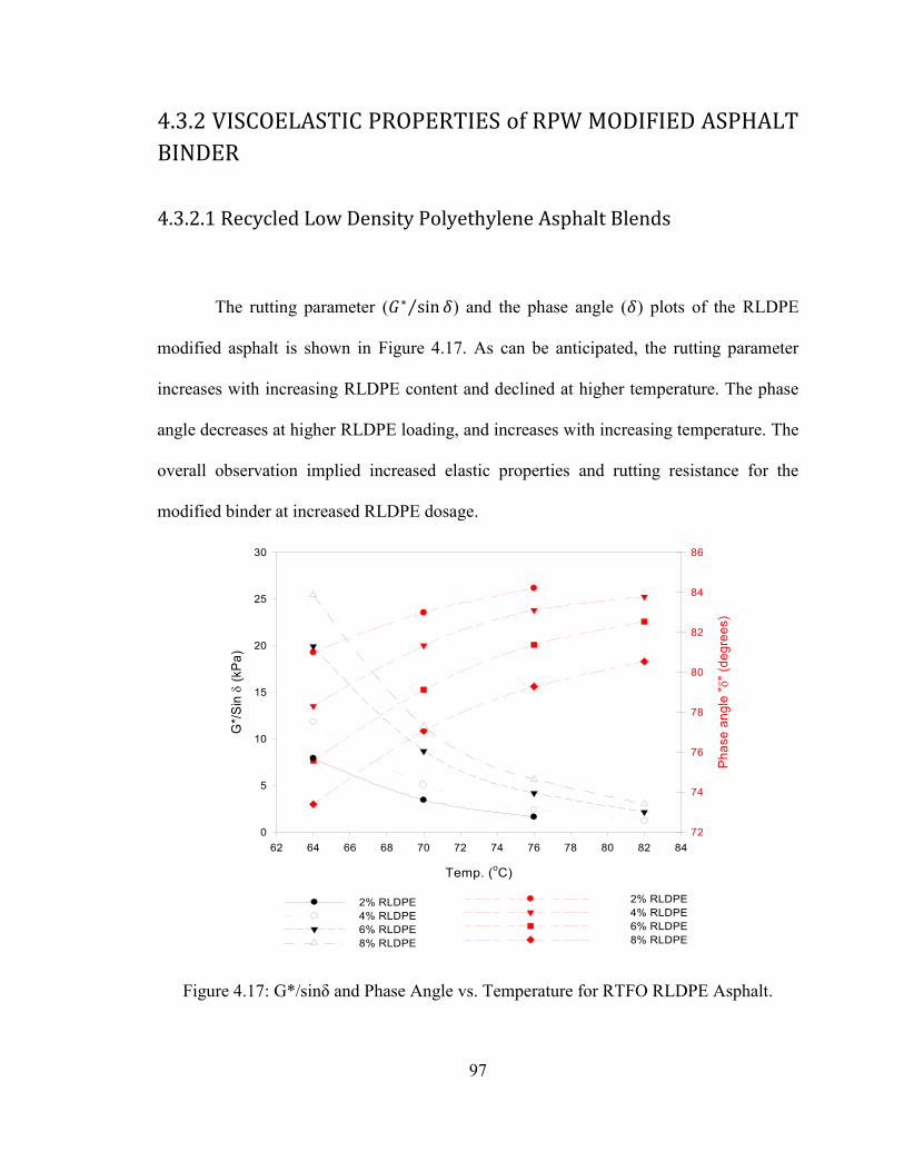
97
4.3.2 VISCOELASTIC PROPERTIES of RPW MODIFIED ASPHALT
BINDER
4.3.2.1 Recycled Low Density Polyethylene Asphalt Blends
The rutting parameter ( ) and the phase angle ( ) plots of the RLDPE
modified asphalt is shown in Figure 4.17. As can be anticipated, the rutting parameter
increases with increasing RLDPE content and declined at higher temperature. The phase
angle decreases at higher RLDPE loading, and increases with increasing temperature. The
overall observation implied increased elastic properties and rutting resistance for the
modified binder at increased RLDPE dosage.
Figure 4.17: G*/sinδ and Phase Angle vs. Temperature for RTFO RLDPE Asphalt.
Pha
se a
ngle
"" (
degr
ees)
72
74
76
78
80
82
84
86
2% RLDPE 4% RLDPE 6% RLDPE 8% RLDPE
Temp. (oC)
62 64 66 68 70 72 74 76 78 80 82 84
G*/
Sin
(k
Pa)
0
5
10
15
20
25
30
2% RLDPE4% RLDPE 6% RLDPE 8% RLDPE
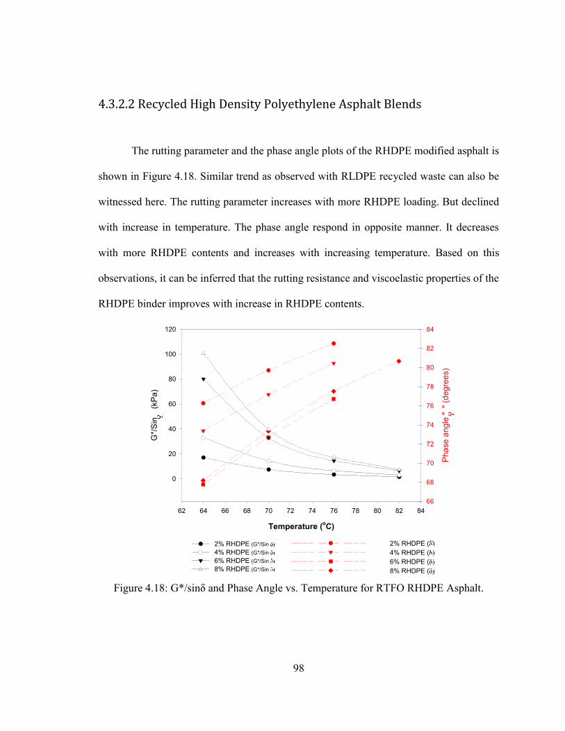
98
4.3.2.2 Recycled High Density Polyethylene Asphalt Blends
The rutting parameter and the phase angle plots of the RHDPE modified asphalt is
shown in Figure 4.18. Similar trend as observed with RLDPE recycled waste can also be
witnessed here. The rutting parameter increases with more RHDPE loading. But declined
with increase in temperature. The phase angle respond in opposite manner. It decreases
with more RHDPE contents and increases with increasing temperature. Based on this
observations, it can be inferred that the rutting resistance and viscoelastic properties of the
RHDPE binder improves with increase in RHDPE contents.
Figure 4.18: G*/sinδ and Phase Angle vs. Temperature for RTFO RHDPE Asphalt.
Pha
se a
ngle
"" (
degr
ees)
66
68
70
72
74
76
78
80
82
84
2% RHDPE (4% RHDPE ( 6% RHDPE (8% RHDPE (
Temperature (oC)
62 64 66 68 70 72 74 76 78 80 82 84
G*/
Sin
(k
Pa)
0
20
40
60
80
100
120
2% RHDPE (G*/Sin 4% RHDPE (G*/Sin 6% RHDPE (G*/Sin 8% RHDPE (G*/Sin
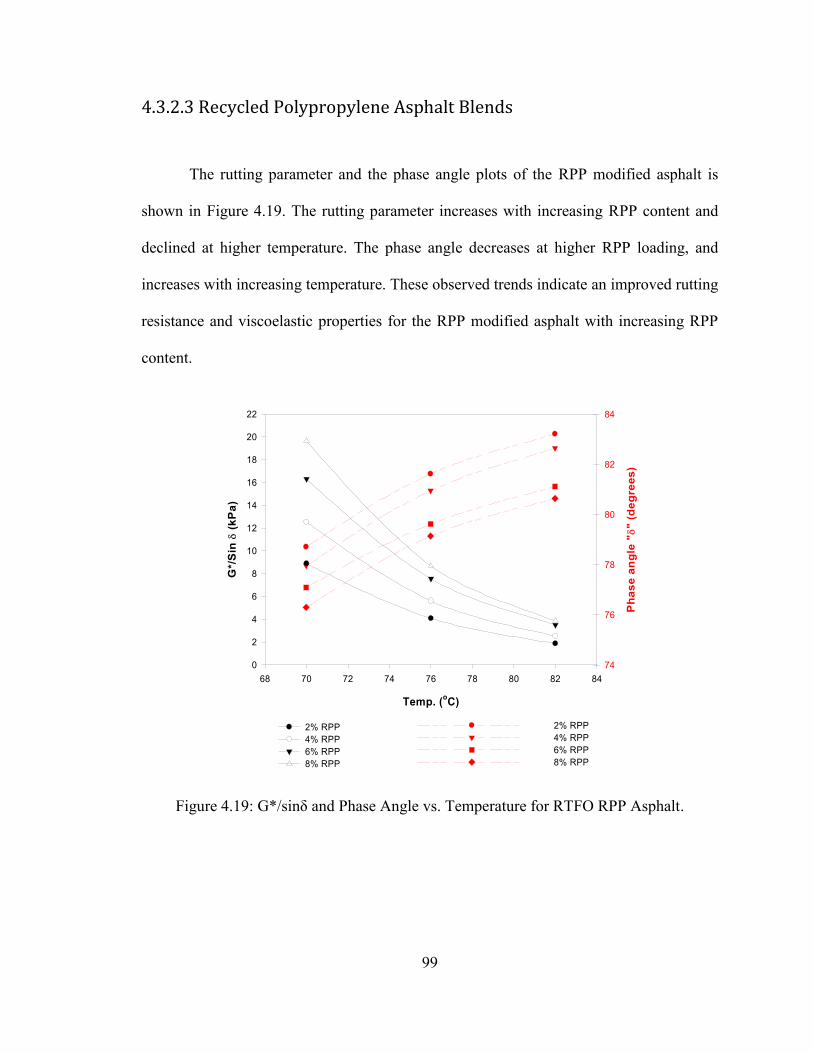
99
4.3.2.3 Recycled Polypropylene Asphalt Blends
The rutting parameter and the phase angle plots of the RPP modified asphalt is
shown in Figure 4.19. The rutting parameter increases with increasing RPP content and
declined at higher temperature. The phase angle decreases at higher RPP loading, and
increases with increasing temperature. These observed trends indicate an improved rutting
resistance and viscoelastic properties for the RPP modified asphalt with increasing RPP
content.
Figure 4.19: G*/sinδ and Phase Angle vs. Temperature for RTFO RPP Asphalt.
Pha
se a
ngle
""
(deg
rees
)
74
76
78
80
82
84
2% RPP4% RPP 6% RPP8% RPP
Temp. (oC)
68 70 72 74 76 78 80 82 84
G*/
Sin
(k
Pa)
0
2
4
6
8
10
12
14
16
18
20
22
2% RPP 4% RPP 6% RPP 8% RPP
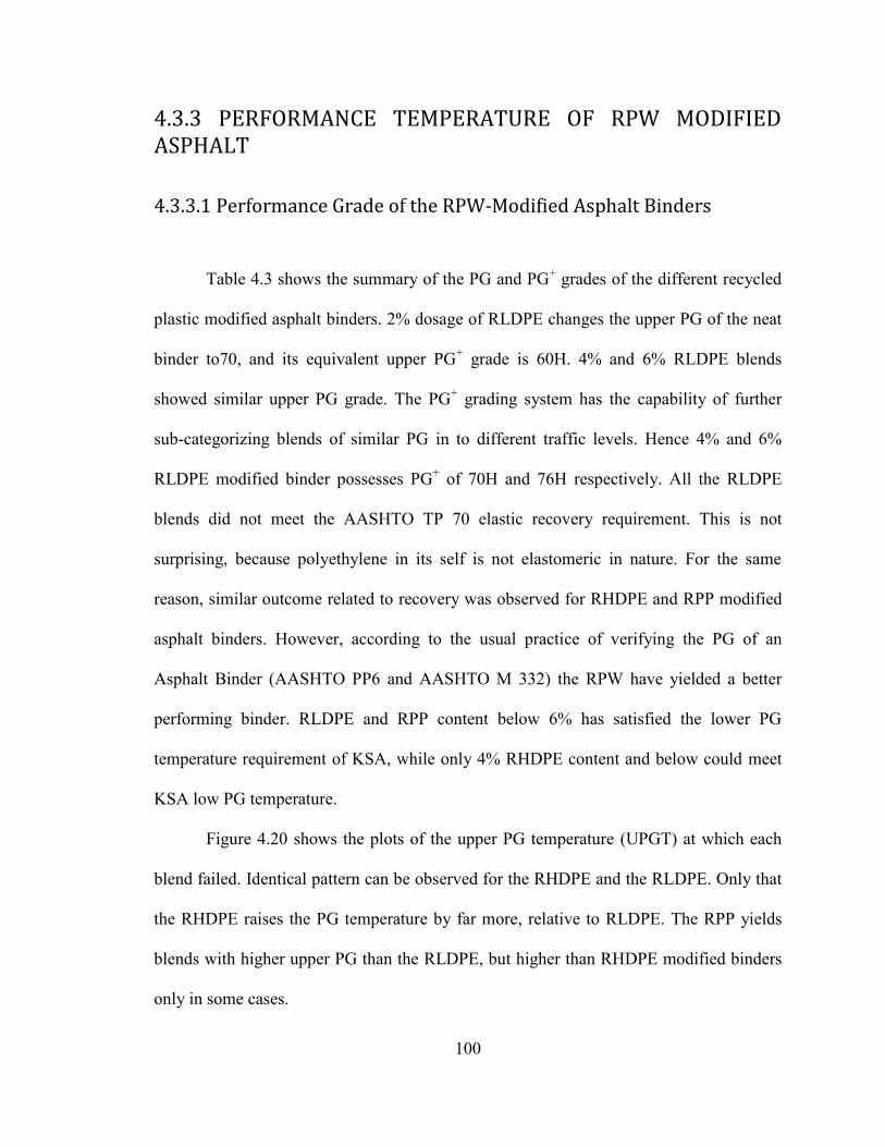
100
4.3.3 PERFORMANCE TEMPERATURE OF RPW MODIFIED ASPHALT
4.3.3.1 Performance Grade of the RPW-Modified Asphalt Binders
Table 4.3 shows the summary of the PG and PG+ grades of the different recycled
plastic modified asphalt binders. 2% dosage of RLDPE changes the upper PG of the neat
binder to70, and its equivalent upper PG+ grade is 60H. 4% and 6% RLDPE blends
showed similar upper PG grade. The PG+ grading system has the capability of further
sub-categorizing blends of similar PG in to different traffic levels. Hence 4% and 6%
RLDPE modified binder possesses PG+ of 70H and 76H respectively. All the RLDPE
blends did not meet the AASHTO TP 70 elastic recovery requirement. This is not
surprising, because polyethylene in its self is not elastomeric in nature. For the same
reason, similar outcome related to recovery was observed for RHDPE and RPP modified
asphalt binders. However, according to the usual practice of verifying the PG of an
Asphalt Binder (AASHTO PP6 and AASHTO M 332) the RPW have yielded a better
performing binder. RLDPE and RPP content below 6% has satisfied the lower PG
temperature requirement of KSA, while only 4% RHDPE content and below could meet
KSA low PG temperature.
Figure 4.20 shows the plots of the upper PG temperature (UPGT) at which each
blend failed. Identical pattern can be observed for the RHDPE and the RLDPE. Only that
the RHDPE raises the PG temperature by far more, relative to RLDPE. The RPP yields
blends with higher upper PG than the RLDPE, but higher than RHDPE modified binders
only in some cases.
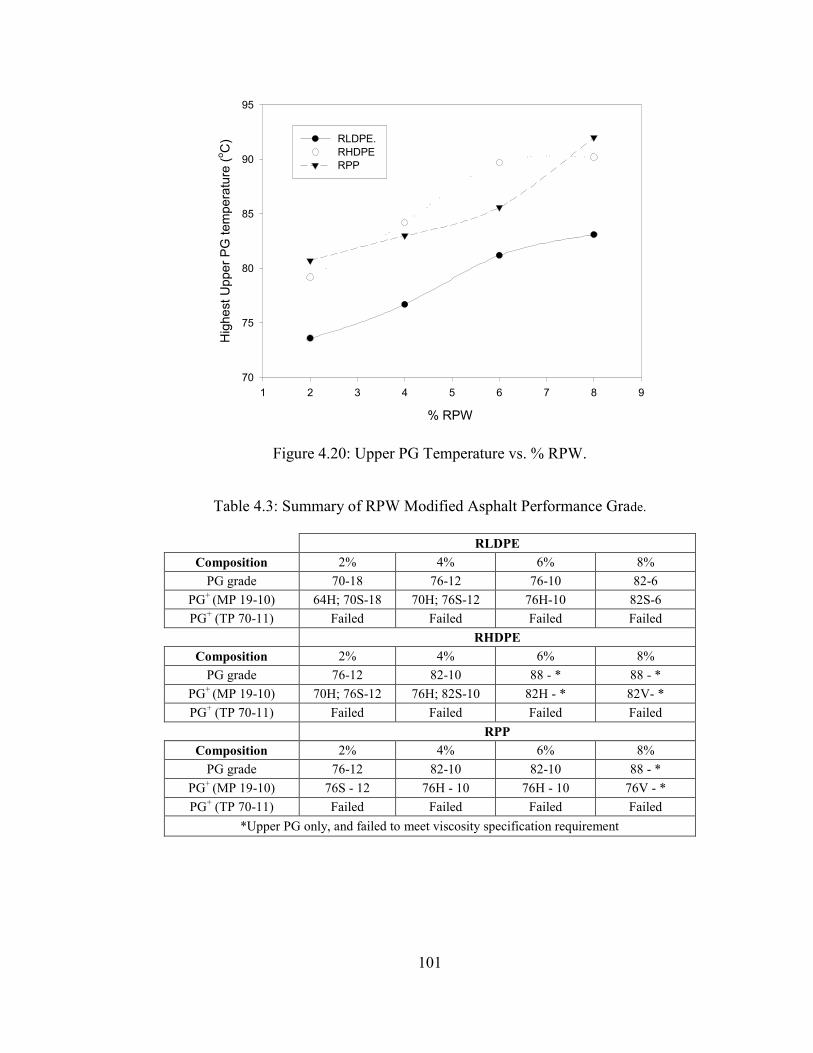
101
Figure 4.20: Upper PG Temperature vs. % RPW.
Table 4.3: Summary of RPW Modified Asphalt Performance Grade.
RLDPE Composition 2% 4% 6% 8%
PG grade 70-18 76-12 76-10 82-6 PG+
(MP 19-10) 64H; 70S-18 70H; 76S-12 76H-10 82S-6 PG+ (TP 70-11) Failed Failed Failed Failed
RHDPE Composition 2% 4% 6% 8%
PG grade 76-12 82-10 88 - * 88 - * PG+
(MP 19-10) 70H; 76S-12 76H; 82S-10 82H - * 82V- * PG+ (TP 70-11) Failed Failed Failed Failed
RPP Composition 2% 4% 6% 8%
PG grade 76-12 82-10 82-10 88 - * PG+
(MP 19-10) 76S - 12 76H - 10 76H - 10 76V - * PG+ (TP 70-11) Failed Failed Failed Failed
*Upper PG only, and failed to meet viscosity specification requirement
% RPW
1 2 3 4 5 6 7 8 9
Hig
hest
Upp
er P
G te
mpe
ratu
re (o C
)
70
75
80
85
90
95
RLDPE. RHDPE RPP
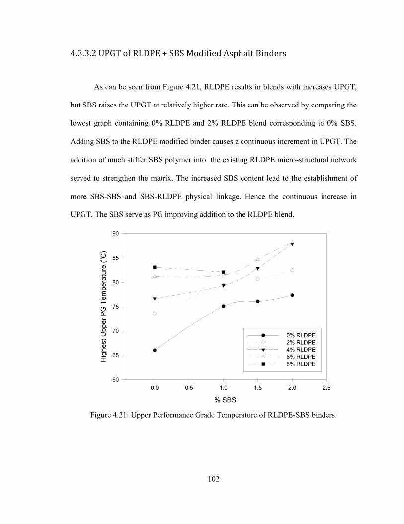
102
4.3.3.2 UPGT of RLDPE + SBS Modified Asphalt Binders
As can be seen from Figure 4.21, RLDPE results in blends with increases UPGT,
but SBS raises the UPGT at relatively higher rate. This can be observed by comparing the
lowest graph containing 0% RLDPE and 2% RLDPE blend corresponding to 0% SBS.
Adding SBS to the RLDPE modified binder causes a continuous increment in UPGT. The
addition of much stiffer SBS polymer into the existing RLDPE micro-structural network
served to strengthen the matrix. The increased SBS content lead to the establishment of
more SBS-SBS and SBS-RLDPE physical linkage. Hence the continuous increase in
UPGT. The SBS serve as PG improving addition to the RLDPE blend.
Figure 4.21: Upper Performance Grade Temperature of RLDPE-SBS binders.
% SBS
0.0 0.5 1.0 1.5 2.0 2.5
Hig
hest
Upp
er P
G T
empe
ratu
re (o C
)
60
65
70
75
80
85
90
0% RLDPE2% RLDPE 4% RLDPE 6% RLDPE 8% RLDPE
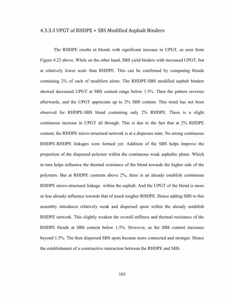
103
4.3.3.3 UPGT of RHDPE + SBS Modified Asphalt Binders
The RHDPE results in blends with significant increase in UPGT, as seen from
Figure 4.22 above. While on the other hand, SBS yield binders with increased UPGT, but
at relatively lower scale than RHDPE. This can be confirmed by comparing blends
containing 2% of each of modifiers alone. The RHDPE-SBS modified asphalt binders
showed decreased UPGT at SBS content range below 1.5%. Then the pattern reverses
afterwards, and the UPGT appreciate up to 2% SBS content. This trend has not been
observed for RHDPE-SBS blend containing only 2% RHDPE. There is a slight
continuous increase in UPGT all through. This is due to the fact that at 2% RHDPE
content, the RHDPE micro-structural network is at a disperses state. No strong continuous
RHDPE-RHDPE linkages were formed yet. Addition of the SBS helps improve the
proportion of the dispersed polymer within the continuous weak asphaltic phase. Which
in turn helps influence the thermal resistance of the blend towards the higher side of the
polymers. But at RHDPE contents above 2%, there is an already establish continuous
RHDPE micro-structural linkage within the asphalt. And the UPGT of the blend is more
or less already influence towards that of much tougher RHDPE. Hence adding SBS to this
assembly introduces relatively weak and dispersed spots within the already establish
RHDPE network. This slightly weaken the overall stiffness and thermal resistance of the
RHDPE blends at SBS content below 1.5%. However, as the SBS content increases
beyond 1.5%. The then dispersed SBS spots became more connected and stronger. Hence
the establishment of a constructive interaction between the RHDPE and SBS.
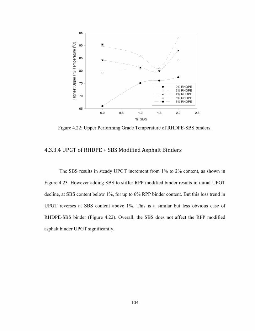
104
Figure 4.22: Upper Performing Grade Temperature of RHDPE-SBS binders.
4.3.3.4 UPGT of RHDPE + SBS Modified Asphalt Binders
The SBS results in steady UPGT increment from 1% to 2% content, as shown in
Figure 4.23. However adding SBS to stiffer RPP modified binder results in initial UPGT
decline, at SBS content below 1%, for up to 6% RPP binder content. But this loss trend in
UPGT reverses at SBS content above 1%. This is a similar but less obvious case of
RHDPE-SBS binder (Figure 4.22). Overall, the SBS does not affect the RPP modified
asphalt binder UPGT significantly.
% SBS
0.0 0.5 1.0 1.5 2.0 2.5
Hig
hest
Upp
er P
G T
empe
ratu
re (o C
)
65
70
75
80
85
90
95
0% RHDPE 2% RHDPE 4% RHDPE 6% RHDPE 8% RHDPE
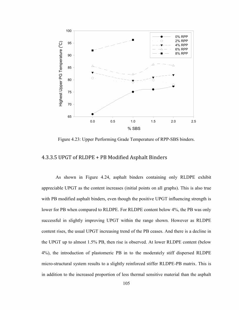
105
Figure 4.23: Upper Performing Grade Temperature of RPP-SBS binders.
4.3.3.5 UPGT of RLDPE + PB Modified Asphalt Binders
As shown in Figure 4.24, asphalt binders containing only RLDPE exhibit
appreciable UPGT as the content increases (initial points on all graphs). This is also true
with PB modified asphalt binders, even though the positive UPGT influencing strength is
lower for PB when compared to RLDPE. For RLDPE content below 4%, the PB was only
successful in slightly improving UPGT within the range shown. However as RLDPE
content rises, the usual UPGT increasing trend of the PB ceases. And there is a decline in
the UPGT up to almost 1.5% PB, then rise is observed. At lower RLDPE content (below
4%), the introduction of plastomeric PB in to the moderately stiff dispersed RLDPE
micro-structural system results to a slightly reinforced stiffer RLDPE-PB matrix. This is
in addition to the increased proportion of less thermal sensitive material than the asphalt
% SBS
0.0 0.5 1.0 1.5 2.0 2.5
Hig
hest
Upp
er P
G T
empe
ratu
re (o C
)
65
70
75
80
85
90
95
100
0% RPP 2% RPP 4% RPP 6% RPP 8% RPP
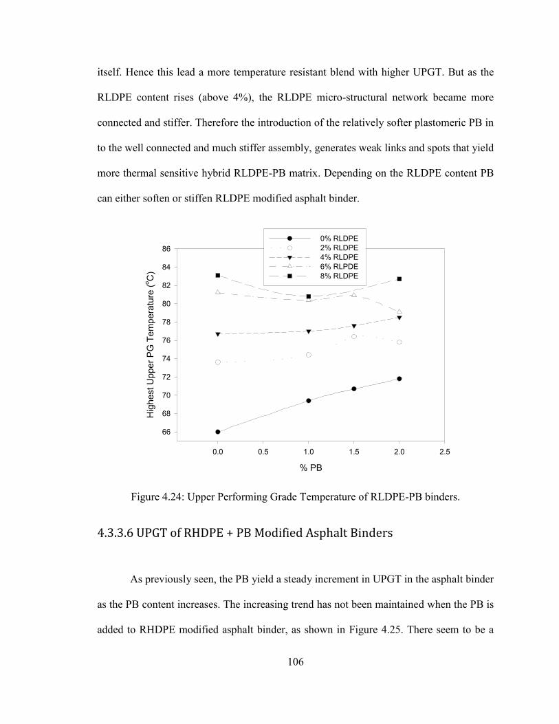
106
itself. Hence this lead a more temperature resistant blend with higher UPGT. But as the
RLDPE content rises (above 4%), the RLDPE micro-structural network became more
connected and stiffer. Therefore the introduction of the relatively softer plastomeric PB in
to the well connected and much stiffer assembly, generates weak links and spots that yield
more thermal sensitive hybrid RLDPE-PB matrix. Depending on the RLDPE content PB
can either soften or stiffen RLDPE modified asphalt binder.
Figure 4.24: Upper Performing Grade Temperature of RLDPE-PB binders.
4.3.3.6 UPGT of RHDPE + PB Modified Asphalt Binders
As previously seen, the PB yield a steady increment in UPGT in the asphalt binder
as the PB content increases. The increasing trend has not been maintained when the PB is
added to RHDPE modified asphalt binder, as shown in Figure 4.25. There seem to be a
% PB
0.0 0.5 1.0 1.5 2.0 2.5
Hig
hest
Upp
er P
G T
empe
ratu
re (o C
)
66
68
70
72
74
76
78
80
82
84
860% RLDPE 2% RLDPE 4% RLDPE 6% RLPDE 8% RLDPE
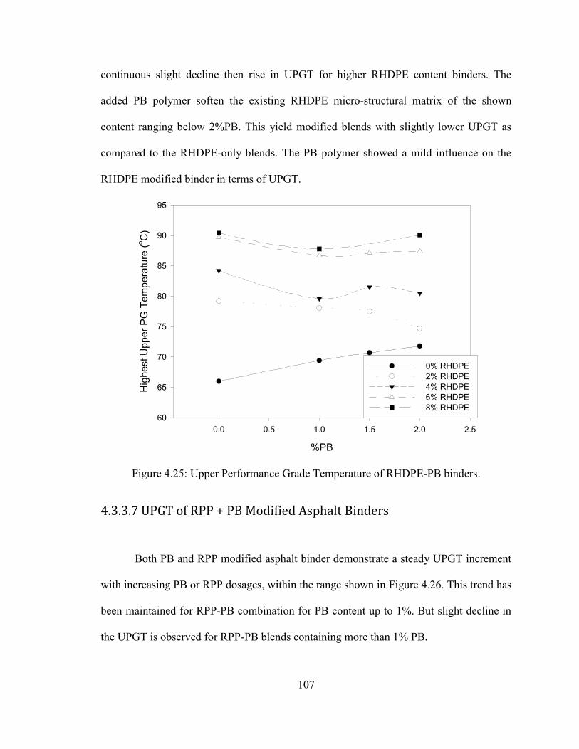
107
continuous slight decline then rise in UPGT for higher RHDPE content binders. The
added PB polymer soften the existing RHDPE micro-structural matrix of the shown
content ranging below 2%PB. This yield modified blends with slightly lower UPGT as
compared to the RHDPE-only blends. The PB polymer showed a mild influence on the
RHDPE modified binder in terms of UPGT.
Figure 4.25: Upper Performance Grade Temperature of RHDPE-PB binders.
4.3.3.7 UPGT of RPP + PB Modified Asphalt Binders
Both PB and RPP modified asphalt binder demonstrate a steady UPGT increment
with increasing PB or RPP dosages, within the range shown in Figure 4.26. This trend has
been maintained for RPP-PB combination for PB content up to 1%. But slight decline in
the UPGT is observed for RPP-PB blends containing more than 1% PB.
%PB
0.0 0.5 1.0 1.5 2.0 2.5
Hig
hest
Upp
er P
G T
empe
ratu
re (o C
)
60
65
70
75
80
85
90
95
0% RHDPE 2% RHDPE 4% RHDPE 6% RHDPE 8% RHDPE
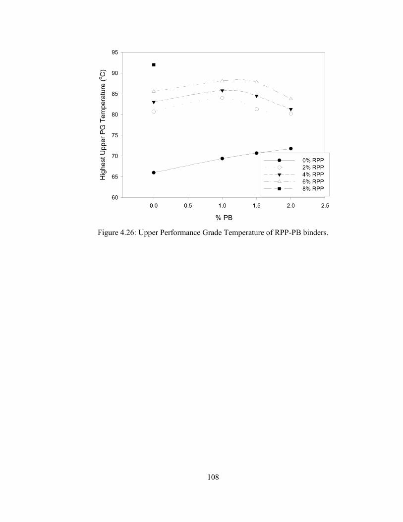
108
Figure 4.26: Upper Performance Grade Temperature of RPP-PB binders.
% PB
0.0 0.5 1.0 1.5 2.0 2.5
Hig
hest
Upp
er P
G T
empe
ratu
re (o C
)
60
65
70
75
80
85
90
95
0% RPP 2% RPP 4% RPP 6% RPP 8% RPP
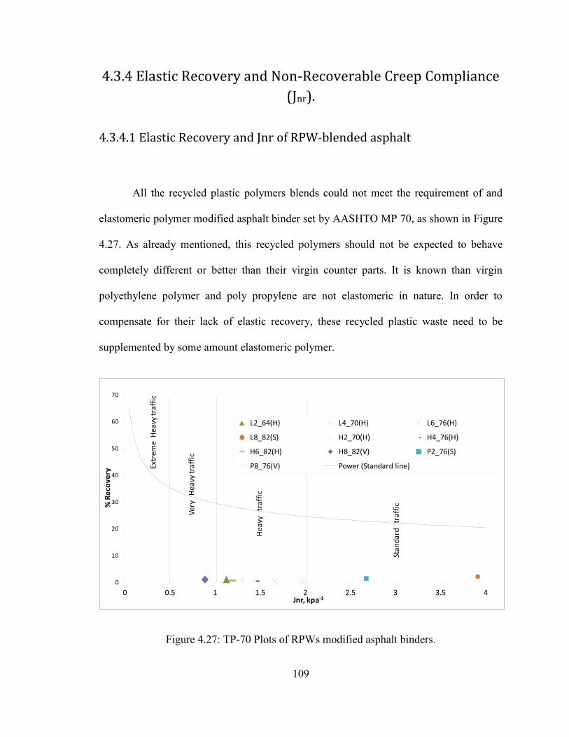
109
4.3.4 Elastic Recovery and Non-Recoverable Creep Compliance
(Jnr).
4.3.4.1 Elastic Recovery and Jnr of RPW-blended asphalt
All the recycled plastic polymers blends could not meet the requirement of and
elastomeric polymer modified asphalt binder set by AASHTO MP 70, as shown in Figure
4.27. As already mentioned, this recycled polymers should not be expected to behave
completely different or better than their virgin counter parts. It is known than virgin
polyethylene polymer and poly propylene are not elastomeric in nature. In order to
compensate for their lack of elastic recovery, these recycled plastic waste need to be
supplemented by some amount elastomeric polymer.
Figure 4.27: TP-70 Plots of RPWs modified asphalt binders.
0
10
20
30
40
50
60
70
0 0.5 1 1.5 2 2.5 3 3.5 4
% R
eco
very
Jnr, kpa-1
L2_64(H) L4_70(H) L6_76(H)
L8_82(S) H2_70(H) H4_76(H)
H6_82(H) H8_82(V) P2_76(S)
P8_76(V) Power (Standard line)Extr
eme
He
avy
traf
fic
Very
H
eavy
traf
fic
Hea
vy
traf
fic
Stan
dard
tr
affi
c
110
4.3.4.2 Elastic Recovery and Jnr of RLDPE-PB modified asphalt binders
Figure 4.28 shows TP_70 plots of RLDPE-PB modified asphalt binders. The
upper plot presents MSCR results obtained at 76oC and the lower plot showed similar
results but obtained at 70oC. It can be seen that the addition of the plastomeric PB to the
RLDPE modified bonder does not add to its recovery, as anticipated. It actually results in
negative recovery due plastic flow especially at 76oC. However, the non recoverable
creep compliance (Jnr) tend to improve and the traffic level of the RLDPE modified
blends is also seen to slightly increase with increasing PB. A typical example is that of
L2PB1_70(S), L2PB1.5_70(H) and L2PB2_70(H) when compared. The RLDPE-PB
binders mostly fall in to standard traffic category at 76oC, while majority are suitable for
heavy and very heavy traffic for 70oC upper PG. In summary, the PB further aggregates
the poor recovery characteristics of RLDPE shown by Figure 4.27, but result in slight Jnr
improvement.
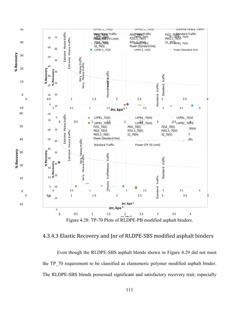
111
Figure 4.28: TP-70 Plots of RLDPE-PB modified asphalt binders.
4.3.4.3 Elastic Recovery and Jnr of RLDPE-SBS modified asphalt binders
Even though the RLDPE-SBS asphalt blends shown in Figure 4.29 did not meet
the TP_70 requirement to be classified as elastomeric polymer modified asphalt binder.
The RLDPE-SBS blends possessed significant and satisfactory recovery trait, especially
-10
0
10
20
30
40
50
60
70
0 0.5 1 1.5 2 2.5 3 3.5 4
% R
eco
ve
ry
L4PB1_76(S) L6PB1_76(S) L8PB1_76(H)
L4PB2_76(S) L6PB2_76(S) L8PB2_76(S)
L2PB1.5_76(S) L4PB1.5_76(S) Power (Standard line)
-10
0
10
20
30
40
50
60
70
0 0.5 1 1.5 2 2.5 3 3.5 4
% R
eco
very
Jnr, kpa-1
L2PB1_70S L4PB1_70(H) L6PB1_70(V)
L8PB1_70(V)" L2PB2_70(H) L4PB2_70(H)
L6PB2_70(V) L8PB2_70(E) L2PB1.5_70(H)
L4PB1.5_(70H) L6PB1.5_70(V) PB1_70(S)
Power (Standard line)
Extr
eme
He
avy
traf
fic
Ve
ry
He
avy
tra
ffic
Hea
vy
traf
fic
Stan
dard
tr
affi
c
Extr
eme
He
avy
traf
fic
Very
H
eavy
traf
fic
He
avy
tra
ffic
Sta
nd
ard
tr
aff
ic
-10
0
10
20
30
40
50
60
0 0.5 1 1.5 2 2.5 3 3.5 4
% R
eco
ve
ry
Jnr, kpa-1
L2PB1_70(S) L4PB1_70(H) L6PB1_70(V)
L8PB1_70(V) L2PB2_70(H) L4PB2_70(H)
L6PB2_70(V) L8PB2_70(E) L2PB1.5_70(H)
L4PB1.5_(70H) L6PB1.5_70(V) PB1_70(S)
Extreme Heavy Traffic Very Heavy Traffic Heavy Traffic
Standard Traffic Power (TP 70 Limit)
-10
0
10
20
30
40
50
60
0 0.5 1 1.5 2 2.5 3 3.5 4
% R
eco
ve
ry
Jnr, kpa-1
L4PB1_76(S) L6PB1_76(S) L8PB1_76(H)
L4PB2_76(S) L6PB2_76(S) L8PB2_76(S)
L2PB1.5_76(S) L4PB1.5_76(S) Extreme Heavy Traffic
Very Heavy Traffic Heavy Traffic Standard Traffic
Power (TP 70 Limit)
0
10
20
30
40
50
60
70
0 0.5 1 1.5 2 2.5 3 3.5 4
% R
eco
ve
ry
P4S1_76(V) P6S1_76(V) P2S1_76(H)P6S2_76(E) P2S1.5_76(V) P6S1.5_76(V)P2S2_76(H) P4S1.5_76(H) S1_76(S)S2_76(S) Power (Standard line)
Extr
em
e H
ea
vy t
raff
ic
Ve
ry H
ea
vy t
raff
ic
He
avy t
raff
ic
Sta
nd
ard
t
raff
ic
Extr
em
e H
ea
vy t
raff
ic
Ve
ry H
ea
vy t
raff
ic
He
avy t
raff
ic
Sta
nd
ard
t
raff
ic
0
10
20
30
40
50
60
70
0 0.5 1 1.5 2 2.5 3 3.5 4
% R
eco
ve
ry
Jnr, kPa-1
P2S1_70(E) P6S1_70(E) P2S2_70(E)P6S2_70(V) P2S1.5_70(E) P4S1.5_70(V)P6S1.5_70(E) S1_70(H) S2_70(V)Power (Standard line)
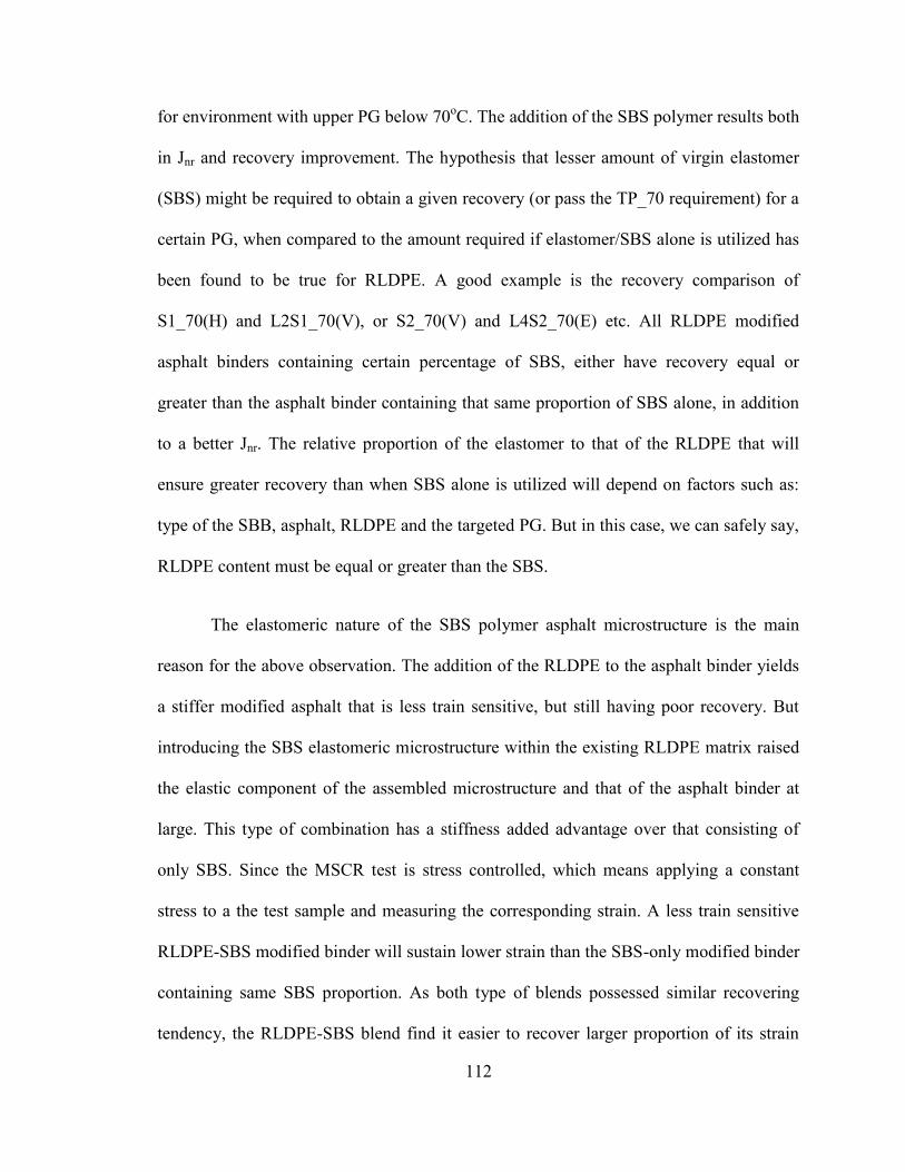
112
for environment with upper PG below 70oC. The addition of the SBS polymer results both
in Jnr and recovery improvement. The hypothesis that lesser amount of virgin elastomer
(SBS) might be required to obtain a given recovery (or pass the TP_70 requirement) for a
certain PG, when compared to the amount required if elastomer/SBS alone is utilized has
been found to be true for RLDPE. A good example is the recovery comparison of
S1_70(H) and L2S1_70(V), or S2_70(V) and L4S2_70(E) etc. All RLDPE modified
asphalt binders containing certain percentage of SBS, either have recovery equal or
greater than the asphalt binder containing that same proportion of SBS alone, in addition
to a better Jnr. The relative proportion of the elastomer to that of the RLDPE that will
ensure greater recovery than when SBS alone is utilized will depend on factors such as:
type of the SBB, asphalt, RLDPE and the targeted PG. But in this case, we can safely say,
RLDPE content must be equal or greater than the SBS.
The elastomeric nature of the SBS polymer asphalt microstructure is the main
reason for the above observation. The addition of the RLDPE to the asphalt binder yields
a stiffer modified asphalt that is less train sensitive, but still having poor recovery. But
introducing the SBS elastomeric microstructure within the existing RLDPE matrix raised
the elastic component of the assembled microstructure and that of the asphalt binder at
large. This type of combination has a stiffness added advantage over that consisting of
only SBS. Since the MSCR test is stress controlled, which means applying a constant
stress to a the test sample and measuring the corresponding strain. A less train sensitive
RLDPE-SBS modified binder will sustain lower strain than the SBS-only modified binder
containing same SBS proportion. As both type of blends possessed similar recovering
tendency, the RLDPE-SBS blend find it easier to recover larger proportion of its strain
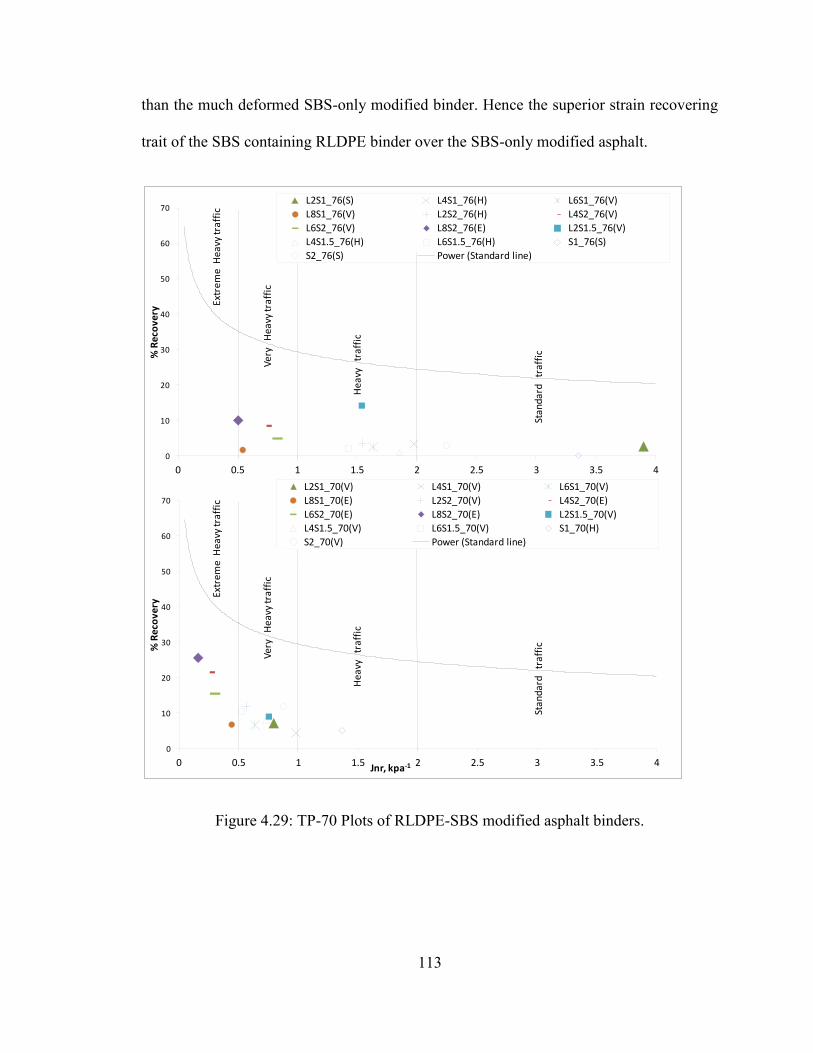
113
than the much deformed SBS-only modified binder. Hence the superior strain recovering
trait of the SBS containing RLDPE binder over the SBS-only modified asphalt.
Figure 4.29: TP-70 Plots of RLDPE-SBS modified asphalt binders.
0
10
20
30
40
50
60
70
0 0.5 1 1.5 2 2.5 3 3.5 4
% R
eco
very
L2S1_76(S) L4S1_76(H) L6S1_76(V)
L8S1_76(V) L2S2_76(H) L4S2_76(V)
L6S2_76(V) L8S2_76(E) L2S1.5_76(V)
L4S1.5_76(H) L6S1.5_76(H) S1_76(S)
S2_76(S) Power (Standard line)
Ext
rem
e H
ea
vy tr
aff
ic
Very
H
eav
y tr
affi
c
He
avy
tra
ffic
Stan
dard
tr
affi
c
Extr
eme
He
avy
traf
fic
Very
H
eav
y tr
affi
c
He
avy
tra
ffic
Stan
dard
tr
affi
c
0
10
20
30
40
50
60
70
0 0.5 1 1.5 2 2.5 3 3.5 4
% R
eco
very
Jnr, kpa-1
L2S1_70(V) L4S1_70(V) L6S1_70(V)
L8S1_70(E) L2S2_70(V) L4S2_70(E)
L6S2_70(E) L8S2_70(E) L2S1.5_70(V)
L4S1.5_70(V) L6S1.5_70(V) S1_70(H)
S2_70(V) Power (Standard line)
114
4.3.4.4 Elastic Recovery and Jnr of RHDPE-PB modified asphalt binders
Figure 4.30 show the TP_70 plots of RHDPE-PB asphalt binders. The
introduction of PB to the RHDPE modified binder has little impact on the recovery. Two
among the three blends with highest recovery as observed from the 70oC results (lower
plot) are highly viscous, as their viscosity results showed (Figure 4.10). Which means
their observed gain in recovery might totally due to their stiff nature, since PB is not
elastomeric polymer. Strain sustained by the less viscous blends is much higher. This
viscous blends regained larger proportion of the relatively lesser strain they underwent.
Most of the RHDPE-PB blends fall between extremely-heavy and very-heavy traffic
category for environment with 70oC upper PG, and between very-heavy and heavy traffic
for environment with upper PG below 76oC.
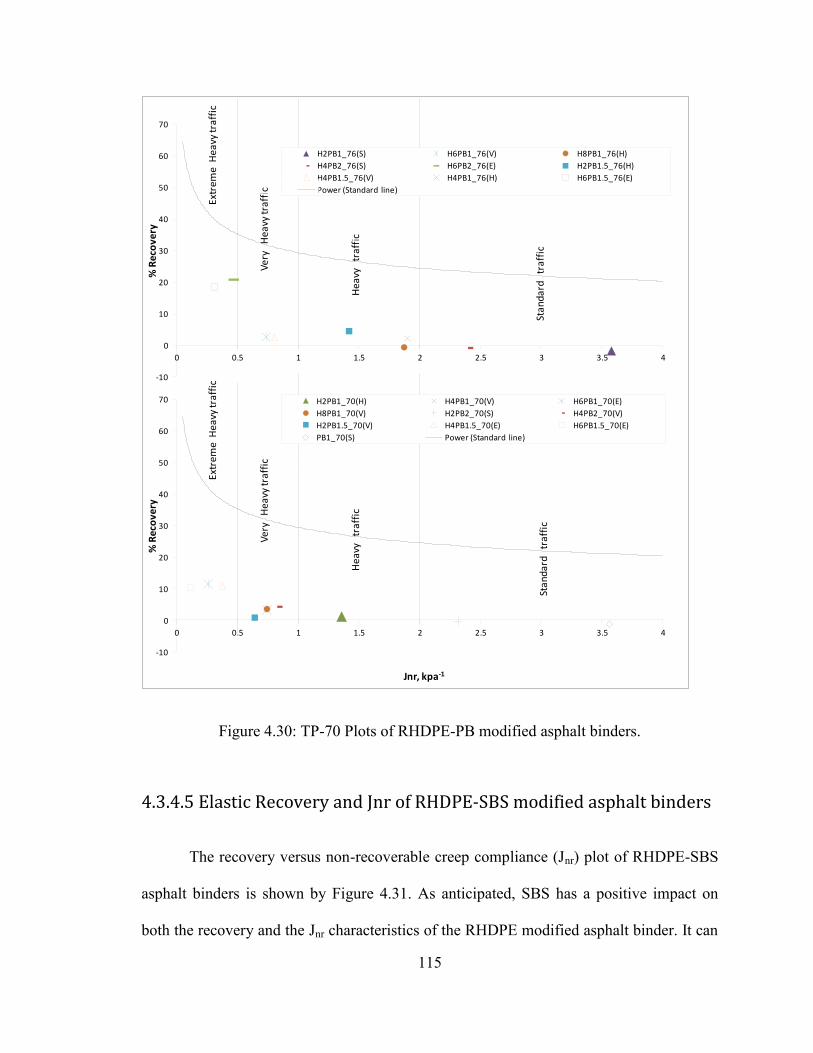
115
Figure 4.30: TP-70 Plots of RHDPE-PB modified asphalt binders.
4.3.4.5 Elastic Recovery and Jnr of RHDPE-SBS modified asphalt binders
The recovery versus non-recoverable creep compliance (Jnr) plot of RHDPE-SBS
asphalt binders is shown by Figure 4.31. As anticipated, SBS has a positive impact on
both the recovery and the Jnr characteristics of the RHDPE modified asphalt binder. It can
-10
0
10
20
30
40
50
60
70
0 0.5 1 1.5 2 2.5 3 3.5 4
% R
eco
very
Jnr, kpa-1
H2PB1_70(H) H4PB1_70(V) H6PB1_70(E)
H8PB1_70(V) H2PB2_70(S) H4PB2_70(V)
H2PB1.5_70(V) H4PB1.5_70(E) H6PB1.5_70(E)
PB1_70(S) Power (Standard line)
Extr
eme
He
avy
traf
fic
Very
H
eavy
traf
fic
Hea
vy
traf
fic
Sta
nd
ard
tr
aff
ic
Extr
eme
Hea
vy tr
affi
c
Very
H
eavy
traf
fic
He
avy
tr
aff
ic
Stan
dard
tr
affi
c
-10
0
10
20
30
40
50
60
70
0 0.5 1 1.5 2 2.5 3 3.5 4
% R
eco
very
H2PB1_76(S) H6PB1_76(V) H8PB1_76(H)
H4PB2_76(S) H6PB2_76(E) H2PB1.5_76(H)
H4PB1.5_76(V) H4PB1_76(H) H6PB1.5_76(E)
Power (Standard line)
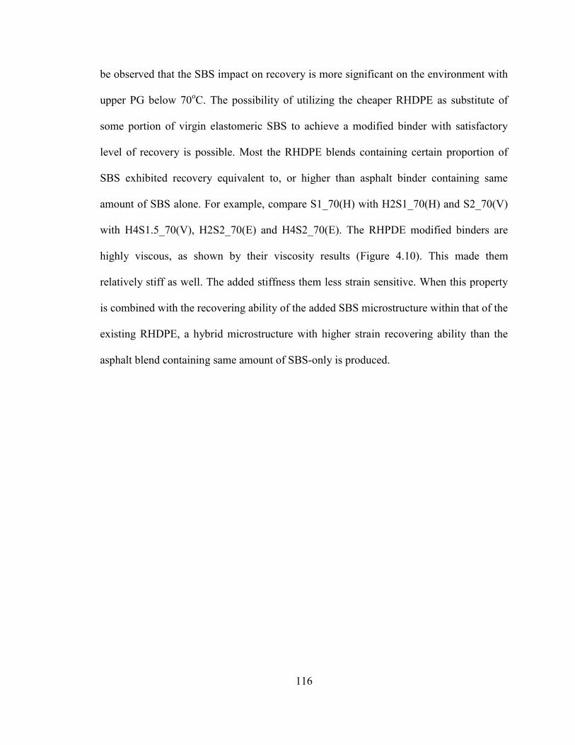
116
be observed that the SBS impact on recovery is more significant on the environment with
upper PG below 70oC. The possibility of utilizing the cheaper RHDPE as substitute of
some portion of virgin elastomeric SBS to achieve a modified binder with satisfactory
level of recovery is possible. Most the RHDPE blends containing certain proportion of
SBS exhibited recovery equivalent to, or higher than asphalt binder containing same
amount of SBS alone. For example, compare S1_70(H) with H2S1_70(H) and S2_70(V)
with H4S1.5_70(V), H2S2_70(E) and H4S2_70(E). The RHPDE modified binders are
highly viscous, as shown by their viscosity results (Figure 4.10). This made them
relatively stiff as well. The added stiffness them less strain sensitive. When this property
is combined with the recovering ability of the added SBS microstructure within that of the
existing RHDPE, a hybrid microstructure with higher strain recovering ability than the
asphalt blend containing same amount of SBS-only is produced.
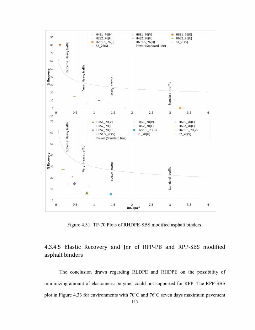
117
Figure 4.31: TP-70 Plots of RHDPE-SBS modified asphalt binders.
4.3.4.5 Elastic Recovery and Jnr of RPP-PB and RPP-SBS modified
asphalt binders
The conclusion drawn regarding RLDPE and RHDPE on the possibility of
minimizing amount of elastomeric polymer could not supported for RPP. The RPP-SBS
plot in Figure 4.33 for environments with 70oC and 76oC seven days maximum pavement
-10
0
10
20
30
40
50
60
70
80
90
0 0.5 1 1.5 2 2.5 3 3.5 4
% R
eco
very
H4S1_76(H) H6S1_76(V) H8S1_76(E)H2S2_76(H) H4S2_76(H) H6S2_76(E)H2S1.5_76(S) H6S1.5_76(H) S1_76(S)S2_76(S) Power (Standard line)
Extr
eme
Hea
vy tr
affi
c
Ver
y H
eav
y tr
affi
c
He
avy
tra
ffic
Stan
dar
d
traf
fic
Extr
eme
Hea
vy tr
affi
c
Very
H
eavy
traf
fic
He
avy
tra
ffic
Stan
dard
tr
affi
c
0
10
20
30
40
50
60
70
0 0.5 1 1.5 2 2.5 3 3.5 4
% R
eco
very
Jnr, kpa-1
H2S1_70(V) H4S1_70(V) H6S1_70(E)H2S2_70(E) H4S2_70(E) H6S2_70(E)H8S2_70(E) H2S1.5_70(H) H4S1.5_70(V)H6S1.5_70(V) S1_70(H) S2_70(V)Power (Standard line)
118
temperature show Jnr and some recovery improvement due to the SBS presence. But no
consistent trend could be observed. This might be attributed to the unstable nature of the
RPP as will be seen in the storage stability section. The RPP-PB modified asphalt results
shown in Figure 4.32 are even more inconsistent than the RPP-SBS results.
Figure 4.32: TP-70 Plots of RPP-PB modified asphalt binders.
0
10
20
30
40
50
60
70
0 0.5 1 1.5 2 2.5 3 3.5 4
% R
eco
very
P4PB1_76(H) P6PB1_76(H) P4PB2_76(S)
P6PB2_76(V) P2PB1.5_76(V) P4PB1.5_76(V)
Power (Standard line)
Ext
rem
e H
ea
vy t
raff
ic
Ve
ry
He
avy
tra
ffic
He
avy
tr
aff
ic
Stan
dard
tr
affi
c
Extr
eme
He
avy
traf
fic
Ver
y H
eav
y tr
affi
c
He
avy
tr
aff
ic
Stan
dard
tr
affi
c
-10
0
10
20
30
40
50
60
70
0 0.5 1 1.5 2 2.5 3 3.5 4
% R
eco
ve
ry
Jnr, kpa-1
P4PB1_70(E) P6PB1_70(E) P8PB1_70(H)
P6PB2_70(H) P2PB1.5_70(E) P4PB1.5_70(E)
6PB1.5_70(E) PB1_70(S) Power (Standard line)
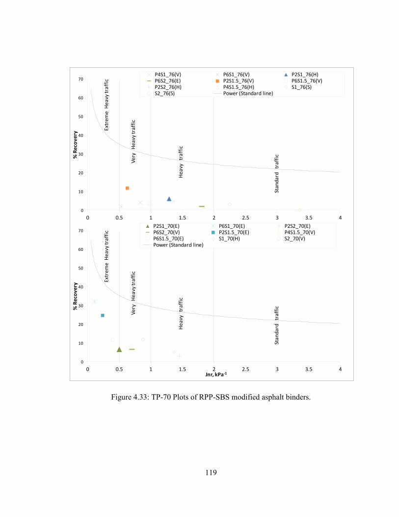
119
Figure 4.33: TP-70 Plots of RPP-SBS modified asphalt binders.
0
10
20
30
40
50
60
70
0 0.5 1 1.5 2 2.5 3 3.5 4
% R
eco
very
P4S1_76(V) P6S1_76(V) P2S1_76(H)P6S2_76(E) P2S1.5_76(V) P6S1.5_76(V)P2S2_76(H) P4S1.5_76(H) S1_76(S)S2_76(S) Power (Standard line)
Extr
eme
He
avy
traf
fic
Very
H
eavy
traf
fic
Hea
vy
traf
fic
Stan
dard
tr
affi
c
Extr
eme
He
avy
traf
fic
Ver
y H
eav
y tr
affi
c
Hea
vy
traf
fic
Stan
dard
tr
affi
c
0
10
20
30
40
50
60
70
0 0.5 1 1.5 2 2.5 3 3.5 4
% R
eco
very
Jnr, kPa-1
P2S1_70(E) P6S1_70(E) P2S2_70(E)P6S2_70(V) P2S1.5_70(E) P4S1.5_70(V)P6S1.5_70(E) S1_70(H) S2_70(V)Power (Standard line)
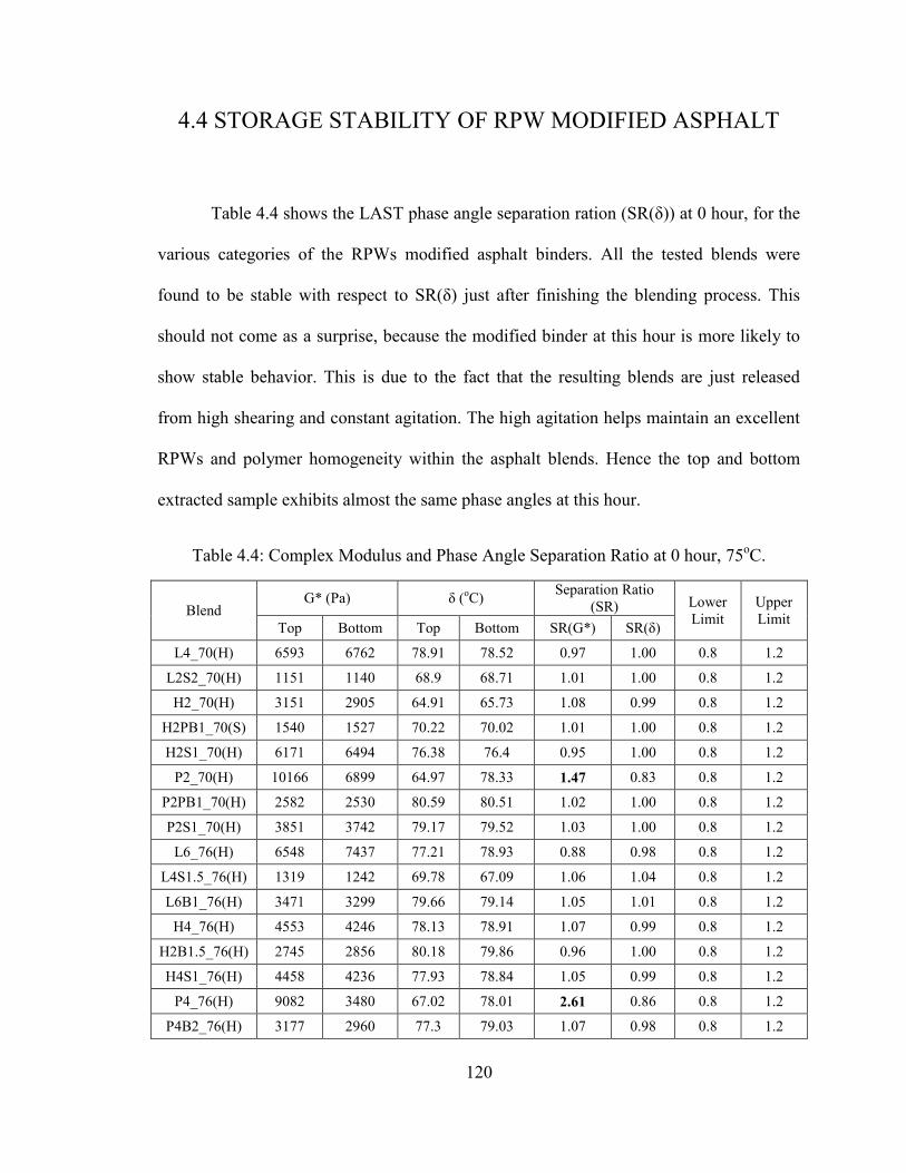
120
4.4 STORAGE STABILITY OF RPW MODIFIED ASPHALT
Table 4.4 shows the LAST phase angle separation ration (SR(δ)) at 0 hour, for the
various categories of the RPWs modified asphalt binders. All the tested blends were
found to be stable with respect to SR(δ) just after finishing the blending process. This
should not come as a surprise, because the modified binder at this hour is more likely to
show stable behavior. This is due to the fact that the resulting blends are just released
from high shearing and constant agitation. The high agitation helps maintain an excellent
RPWs and polymer homogeneity within the asphalt blends. Hence the top and bottom
extracted sample exhibits almost the same phase angles at this hour.
Table 4.4: Complex Modulus and Phase Angle Separation Ratio at 0 hour, 75oC.
Blend G* (Pa) δ (oC) Separation Ratio
(SR) Lower Limit
Upper Limit Top Bottom Top Bottom SR(G*) SR(δ)
L4_70(H) 6593 6762 78.91 78.52 0.97 1.00 0.8 1.2
L2S2_70(H) 1151 1140 68.9 68.71 1.01 1.00 0.8 1.2
H2_70(H) 3151 2905 64.91 65.73 1.08 0.99 0.8 1.2
H2PB1_70(S) 1540 1527 70.22 70.02 1.01 1.00 0.8 1.2
H2S1_70(H) 6171 6494 76.38 76.4 0.95 1.00 0.8 1.2
P2_70(H) 10166 6899 64.97 78.33 1.47 0.83 0.8 1.2
P2PB1_70(H) 2582 2530 80.59 80.51 1.02 1.00 0.8 1.2
P2S1_70(H) 3851 3742 79.17 79.52 1.03 1.00 0.8 1.2
L6_76(H) 6548 7437 77.21 78.93 0.88 0.98 0.8 1.2
L4S1.5_76(H) 1319 1242 69.78 67.09 1.06 1.04 0.8 1.2
L6B1_76(H) 3471 3299 79.66 79.14 1.05 1.01 0.8 1.2
H4_76(H) 4553 4246 78.13 78.91 1.07 0.99 0.8 1.2
H2B1.5_76(H) 2745 2856 80.18 79.86 0.96 1.00 0.8 1.2
H4S1_76(H) 4458 4236 77.93 78.84 1.05 0.99 0.8 1.2
P4_76(H) 9082 3480 67.02 78.01 2.61 0.86 0.8 1.2
P4B2_76(H) 3177 2960 77.3 79.03 1.07 0.98 0.8 1.2
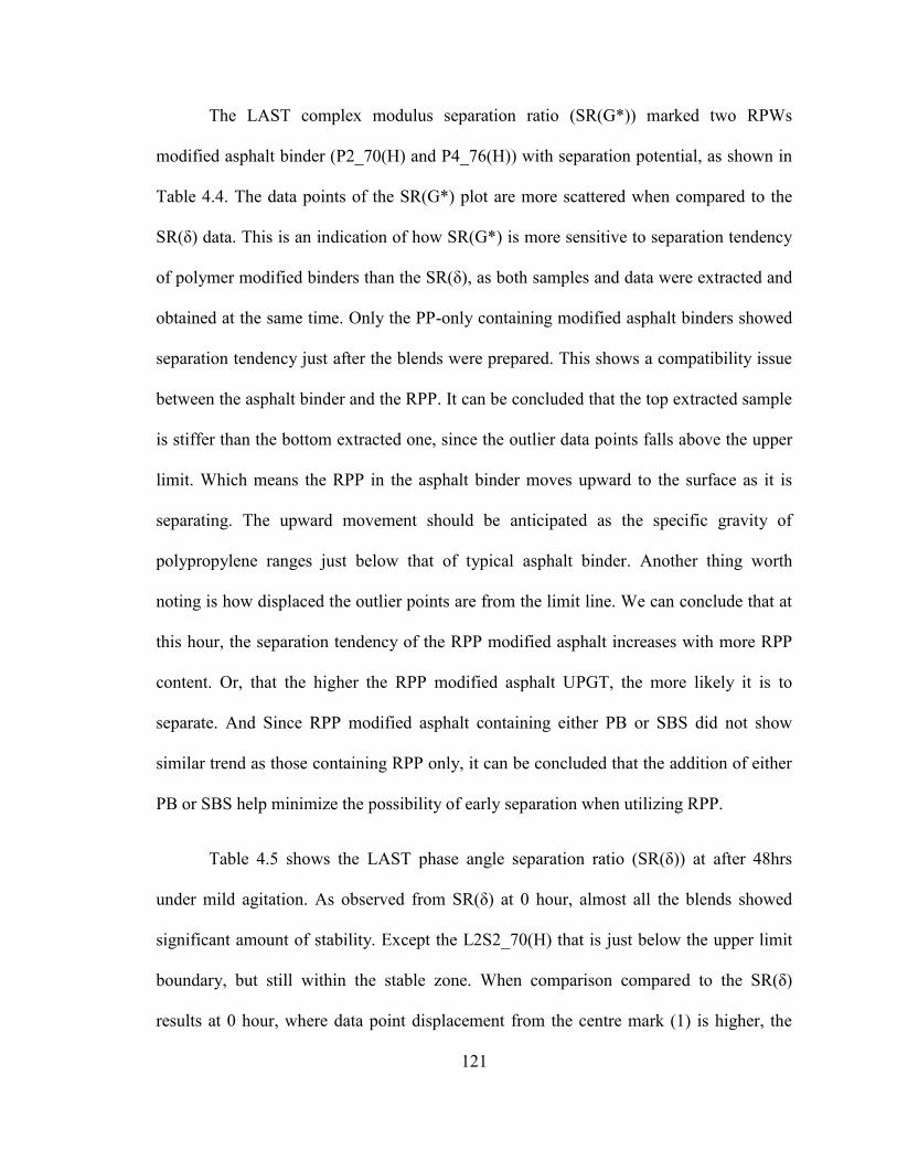
121
The LAST complex modulus separation ratio (SR(G*)) marked two RPWs
modified asphalt binder (P2_70(H) and P4_76(H)) with separation potential, as shown in
Table 4.4. The data points of the SR(G*) plot are more scattered when compared to the
SR(δ) data. This is an indication of how SR(G*) is more sensitive to separation tendency
of polymer modified binders than the SR(δ), as both samples and data were extracted and
obtained at the same time. Only the PP-only containing modified asphalt binders showed
separation tendency just after the blends were prepared. This shows a compatibility issue
between the asphalt binder and the RPP. It can be concluded that the top extracted sample
is stiffer than the bottom extracted one, since the outlier data points falls above the upper
limit. Which means the RPP in the asphalt binder moves upward to the surface as it is
separating. The upward movement should be anticipated as the specific gravity of
polypropylene ranges just below that of typical asphalt binder. Another thing worth
noting is how displaced the outlier points are from the limit line. We can conclude that at
this hour, the separation tendency of the RPP modified asphalt increases with more RPP
content. Or, that the higher the RPP modified asphalt UPGT, the more likely it is to
separate. And Since RPP modified asphalt containing either PB or SBS did not show
similar trend as those containing RPP only, it can be concluded that the addition of either
PB or SBS help minimize the possibility of early separation when utilizing RPP.
Table 4.5 shows the LAST phase angle separation ratio (SR(δ)) at after 48hrs
under mild agitation. As observed from SR(δ) at 0 hour, almost all the blends showed
significant amount of stability. Except the L2S2_70(H) that is just below the upper limit
boundary, but still within the stable zone. When comparison compared to the SR(δ)
results at 0 hour, where data point displacement from the centre mark (1) is higher, the
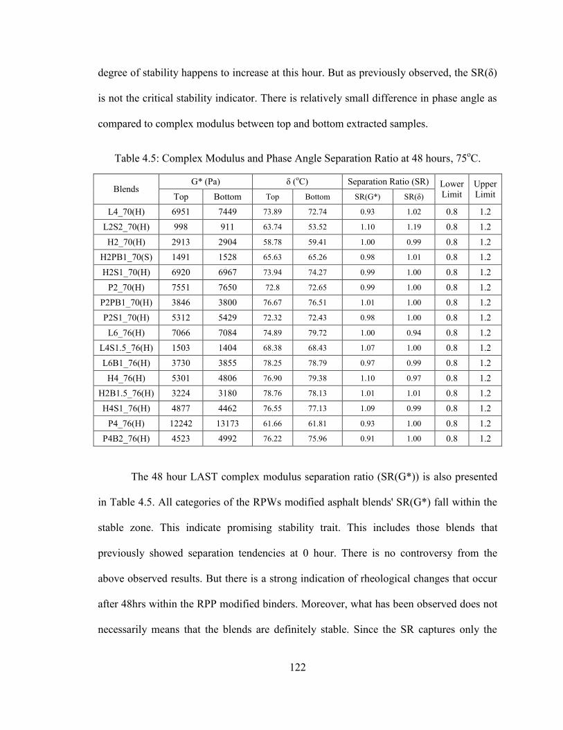
122
degree of stability happens to increase at this hour. But as previously observed, the SR(δ)
is not the critical stability indicator. There is relatively small difference in phase angle as
compared to complex modulus between top and bottom extracted samples.
Table 4.5: Complex Modulus and Phase Angle Separation Ratio at 48 hours, 75oC.
Blends G* (Pa) δ (oC) Separation Ratio (SR) Lower
Limit Upper Limit Top Bottom Top Bottom SR(G*) SR(δ)
L4_70(H) 6951 7449 73.89 72.74 0.93 1.02 0.8 1.2
L2S2_70(H) 998 911 63.74 53.52 1.10 1.19 0.8 1.2
H2_70(H) 2913 2904 58.78 59.41 1.00 0.99 0.8 1.2 H2PB1_70(S) 1491 1528 65.63 65.26 0.98 1.01 0.8 1.2
H2S1_70(H) 6920 6967 73.94 74.27 0.99 1.00 0.8 1.2
P2_70(H) 7551 7650 72.8 72.65 0.99 1.00 0.8 1.2 P2PB1_70(H) 3846 3800 76.67 76.51 1.01 1.00 0.8 1.2
P2S1_70(H) 5312 5429 72.32 72.43 0.98 1.00 0.8 1.2
L6_76(H) 7066 7084 74.89 79.72 1.00 0.94 0.8 1.2 L4S1.5_76(H) 1503 1404 68.38 68.43 1.07 1.00 0.8 1.2
L6B1_76(H) 3730 3855 78.25 78.79 0.97 0.99 0.8 1.2
H4_76(H) 5301 4806 76.90 79.38 1.10 0.97 0.8 1.2 H2B1.5_76(H) 3224 3180 78.76 78.13 1.01 1.01 0.8 1.2
H4S1_76(H) 4877 4462 76.55 77.13 1.09 0.99 0.8 1.2
P4_76(H) 12242 13173 61.66 61.81 0.93 1.00 0.8 1.2 P4B2_76(H) 4523 4992 76.22 75.96 0.91 1.00 0.8 1.2
The 48 hour LAST complex modulus separation ratio (SR(G*)) is also presented
in Table 4.5. All categories of the RPWs modified asphalt blends' SR(G*) fall within the
stable zone. This indicate promising stability trait. This includes those blends that
previously showed separation tendencies at 0 hour. There is no controversy from the
above observed results. But there is a strong indication of rheological changes that occur
after 48hrs within the RPP modified binders. Moreover, what has been observed does not
necessarily means that the blends are definitely stable. Since the SR captures only the
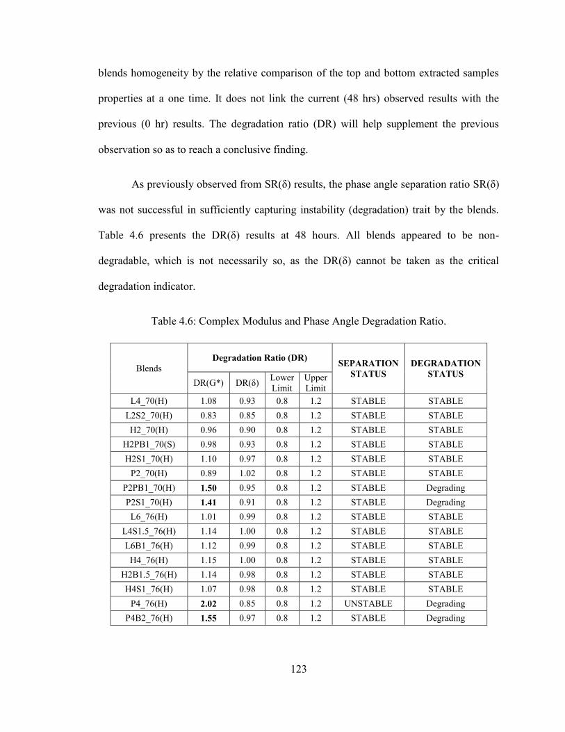
123
blends homogeneity by the relative comparison of the top and bottom extracted samples
properties at a one time. It does not link the current (48 hrs) observed results with the
previous (0 hr) results. The degradation ratio (DR) will help supplement the previous
observation so as to reach a conclusive finding.
As previously observed from SR(δ) results, the phase angle separation ratio SR(δ)
was not successful in sufficiently capturing instability (degradation) trait by the blends.
Table 4.6 presents the DR(δ) results at 48 hours. All blends appeared to be non-
degradable, which is not necessarily so, as the DR(δ) cannot be taken as the critical
degradation indicator.
Table 4.6: Complex Modulus and Phase Angle Degradation Ratio.
Blends Degradation Ratio (DR) SEPARATION
STATUS DEGRADATION
STATUS DR(G*) DR(δ) Lower
Limit Upper Limit
L4_70(H) 1.08 0.93 0.8 1.2 STABLE STABLE L2S2_70(H) 0.83 0.85 0.8 1.2 STABLE STABLE H2_70(H) 0.96 0.90 0.8 1.2 STABLE STABLE
H2PB1_70(S) 0.98 0.93 0.8 1.2 STABLE STABLE H2S1_70(H) 1.10 0.97 0.8 1.2 STABLE STABLE
P2_70(H) 0.89 1.02 0.8 1.2 STABLE STABLE P2PB1_70(H) 1.50 0.95 0.8 1.2 STABLE Degrading P2S1_70(H) 1.41 0.91 0.8 1.2 STABLE Degrading
L6_76(H) 1.01 0.99 0.8 1.2 STABLE STABLE L4S1.5_76(H) 1.14 1.00 0.8 1.2 STABLE STABLE L6B1_76(H) 1.12 0.99 0.8 1.2 STABLE STABLE
H4_76(H) 1.15 1.00 0.8 1.2 STABLE STABLE H2B1.5_76(H) 1.14 0.98 0.8 1.2 STABLE STABLE H4S1_76(H) 1.07 0.98 0.8 1.2 STABLE STABLE
P4_76(H) 2.02 0.85 0.8 1.2 UNSTABLE Degrading P4B2_76(H) 1.55 0.97 0.8 1.2 STABLE Degrading
124
Table 4.6 also presents the complex modulus degradation ratio (DR(G*)) at 48 hours. As
can be observed, not all the RPWs modified asphalt binders' DR(G*) fall within the
acceptable degradation zone. Four blends (P2PB1_70(H), P2S1_70(H), P4_76(H), and
P4PB2_76(H)) were found to show potential degradation trait with time during storage.
As in the case of separation, the more the RPP content the higher degradation tendency.
The higher the RPP content the further away the DR(G*) seemed from the upper
acceptable limits (1.2). Micro-structural reorganization and possible time hardening due
to continuous agitation is what could have led to the significant difference in the visco-
elastic property between the sample extracted just after blending and those after 48 hours
of mild agitation. Because none of the affected blends showed significant difference
between top and bottom samples' visco-elastic properties at 48th hour. They have all
passed the separation criteria. The early separation attribute of RPP modified asphalt
binder is only seen on P2_70(H) and P4_76(H) SR(G*) plot at 0 hour (Table 4.4).
However, RPP asphalt blends containing either SBS or PB did not show this behavior.
The presence of extra SBS or PB micro-structural network within the RPP blend tend to
slow the rate at which the RPP micro-structure reorganizes to move towards the asphalt
surface. The only blend that failed to meet the separation criteria at 0 hour, but has met
the degradation requirement is P2_70(H).
Hence, we can conclude that P2PB1_70(H), P2S1_70(H), P4_76(H), and P4PB2_76(H)
are unstable due to their degrading tendency with time. P2_70(H) is only stable under
mild agitation. RPP content above 2% will lead to an unstable modified asphalt binder.
Addition of an elastomeric SBS and Plastomeric PB minimize the early separation of RPP

125
modified asphalt binder, but does not necessarily mean they are stable. As they have
shown a potential degrading tendency with time. RHDPE and RLDPE modified asphalt
binders (for RHDPE content below 4% and RLDPE content below 6%) whether
containing either SBS or PB have shown good storage stability trait under mild agitation,
both in terms of time degradation and separation.
126
4.5 COMPOSITION OF RPW IN THE RPW-ASPHALT
CONCRETE
The bulk combination of the plastic wastes was employed for the AC aggregate
substitution due to economic and practical reasons. Huge amount of the RPW is required
for aggregate replacement in AC, and the cost associated with sorting the RPW into their
categories is high and impractical. Besides, unlike in the case of asphalt binder
modification, all the RPW are eligible for use as aggregate replacement. The summary of
the pilot survey results of household waste on the various composition of the combined
RPW is shown in Table 4.7. The combined RPW waste from households in Thuqba and
Doha, Dhahran KSA was estimated to approximately consist of 33.7% PET, 25% HDPE,
3.8% PVC, 17.1% LDPE, 11.6% PP and 8.8% PS. The sample size required for a much
reliable proportion estimate at 5 and 10% level of statistical significance was calculated
from this survey. This can be observed that more sampling is required for a reliable data.
However, since what was needed for this research is just an estimate, this results will
suffice. The upper and lower confidence bound (UCB and LCB) for these estimated
proportions is also estimated. Typical image of the combined RPW for AC modification
via aggregate substitution is shown in Figure 4.34.
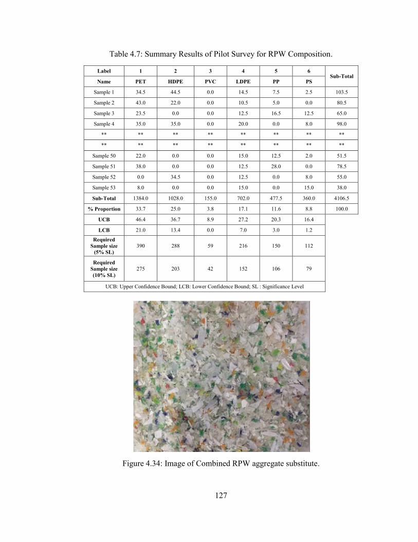
127
Table 4.7: Summary Results of Pilot Survey for RPW Composition.
Label 1 2 3 4 5 6 Sub-Total
Name PET HDPE PVC LDPE PP PS
Sample 1 34.5 44.5 0.0 14.5 7.5 2.5 103.5
Sample 2 43.0 22.0 0.0 10.5 5.0 0.0 80.5
Sample 3 23.5 0.0 0.0 12.5 16.5 12.5 65.0
Sample 4 35.0 35.0 0.0 20.0 0.0 8.0 98.0
** ** ** ** ** ** ** **
** ** ** ** ** ** ** **
Sample 50 22.0 0.0 0.0 15.0 12.5 2.0 51.5
Sample 51 38.0 0.0 0.0 12.5 28.0 0.0 78.5
Sample 52 0.0 34.5 0.0 12.5 0.0 8.0 55.0
Sample 53 8.0 0.0 0.0 15.0 0.0 15.0 38.0
Sub-Total 1384.0 1028.0 155.0 702.0 477.5 360.0 4106.5
% Proportion 33.7 25.0 3.8 17.1 11.6 8.8 100.0
UCB 46.4 36.7 8.9 27.2 20.3 16.4 LCB 21.0 13.4 0.0 7.0 3.0 1.2
Required Sample size
(5% SL) 390 288 59 216 150 112
Required Sample size (10% SL)
275 203 42 152 106 79
UCB: Upper Confidence Bound; LCB: Lower Confidence Bound; SL : Significance Level
Figure 4.34: Image of Combined RPW aggregate substitute.
128
4.6 SUPERPAVE MIX DESIGN RESULTS OF RPW-ASPHALT
CONCRETE MIX
4.6.1 Compaction and Mixing Temperature
The relationship between the RPW asphalt binder viscosities and temperature was
established and presented in Figure 4.35. The recommended mixing and compaction
asphalt viscosity ranges are 0.17 ± 0.02 and 0.28 ± 0.03 Pas, respectively. The mixing and
compaction temperature for the various RPW asphalt binders were obtained within this
range from the viscosity-temperature plots shown in Figure 4.35. The flow activation
energy 'E' of the RPW-binders, a measure of required compaction effort related to the
viscosity of the binder was obtained from Arrhenius equation (42) and presented in the
Table 4.8. It can be observed that the flow activation energy of the various RPW-asphalt
are not far from that of the crumb rubber binder. The H4 and P2S1.5 binders showed the
highest required compaction energy when compared to the rest of the binders at the
temperature. It can be concluded that all the RPW asphalt binder mixtures, with the
exception of H2B1.5, will require a slightly higher compaction effort than the crumb
rubber mix at the same temperature.
(4.1)
Where: : viscosity (Pa.s), : Temperature (oK), : flow activation energy,
and A is the plot intercept.
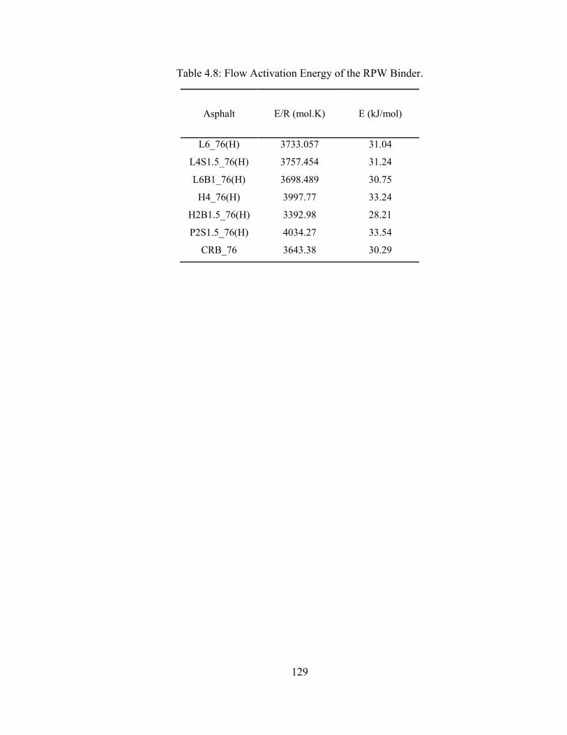
129
Table 4.8: Flow Activation Energy of the RPW Binder.
Asphalt E/R (mol.K) E (kJ/mol)
L6_76(H) 3733.057 31.04
L4S1.5_76(H) 3757.454 31.24
L6B1_76(H) 3698.489 30.75
H4_76(H) 3997.77 33.24
H2B1.5_76(H) 3392.98 28.21
P2S1.5_76(H) 4034.27 33.54
CRB_76 3643.38 30.29
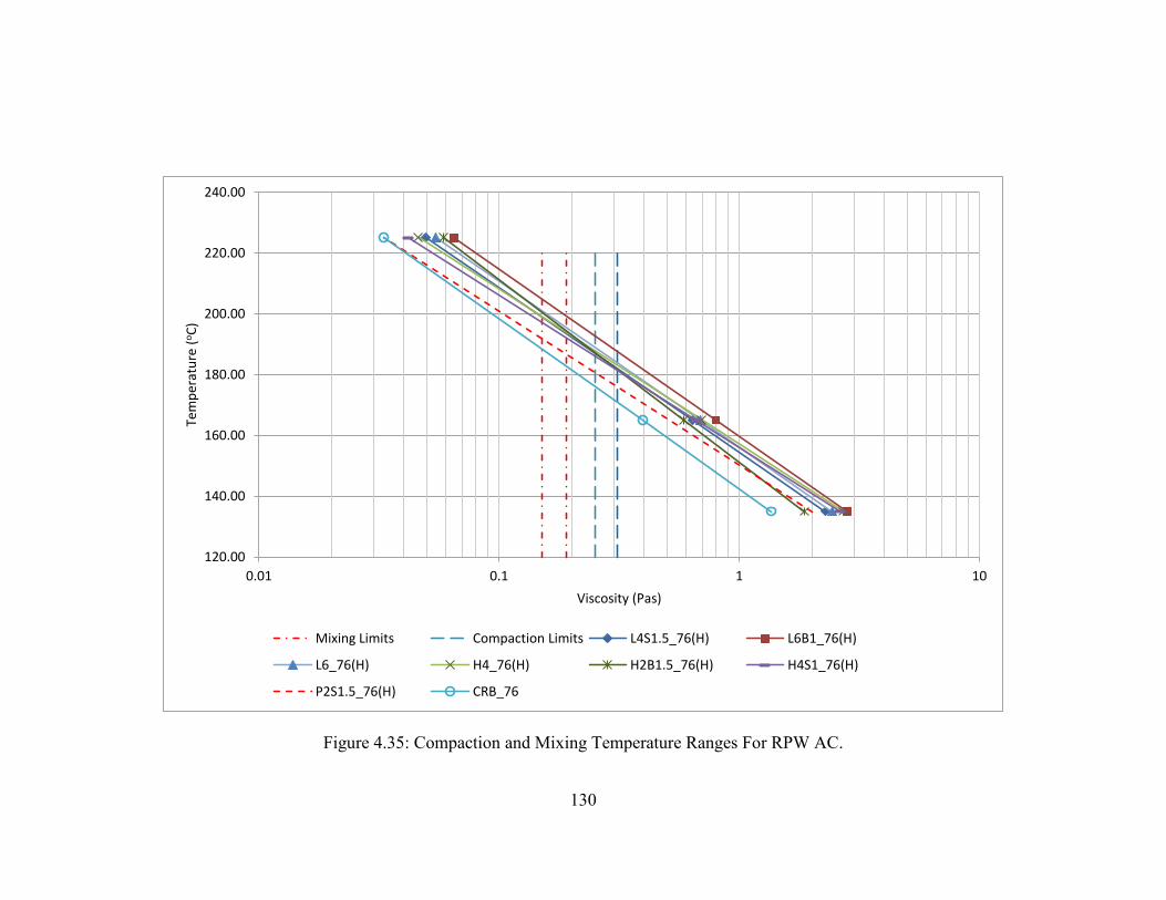
130
Figure 4.35: Compaction and Mixing Temperature Ranges For RPW AC.
120.00
140.00
160.00
180.00
200.00
220.00
240.00
0.01 0.1 1 10
Tem
per
atu
re (
oC
)
Viscosity (Pas)
Mixing Limits Compaction Limits L4S1.5_76(H) L6B1_76(H)
L6_76(H) H4_76(H) H2B1.5_76(H) H4S1_76(H)
P2S1.5_76(H) CRB_76
131
4.6.2 Mix Design Summary and RPW-AC Mixtures Parameters
Table 4.9 present the selection of aggregate gradation results for L6_76(H). The
criteria are air void, void in mineral aggregate (VMA), void filled with asphalt (VFA),
level of compaction relative to the maximum theoretical density (%Gmm) at three stages of
the pavement life, namely Ndesign, Ninitial and Nmax. Three trial gradations G1, G2, and G3
(Table 3.6) were checked, and G1 happened to be the best option based on the design
criteria. G1 yielded a mix with air void, VFA, VMA and level of compaction much closer
to the target criteria than both G2 and G3. The G1 gradation was selected for the optimum
asphalt binder content determination phase. Similar approach was employed for the
remaining AC mixtures.
Due to the unstable nature of the RPP modified binder, only the P2S1.5 binder
was selected for AC mix design phase, just for reference purpose. The summary of the
superpave mix design of the RPW asphalt concretes was presented in Table 4.10. All the
important volumetric properties of the mixtures such as the VMA, VFA, optimum asphalt
content and selected gradation, percent maximum theoretical density (Gmm) at Ndesign,
Ninitial and Nmax, in addition to the mixing and compaction temperature for each mix were
outlined. The moisture durability test result for the mixtures is shown in Figure 4.36. All
the RPW modified asphalt mixture met the minimum retained strength index (RSI) of
80%, with the L6_(76) mix retaining almost all its indirect tensile strength.
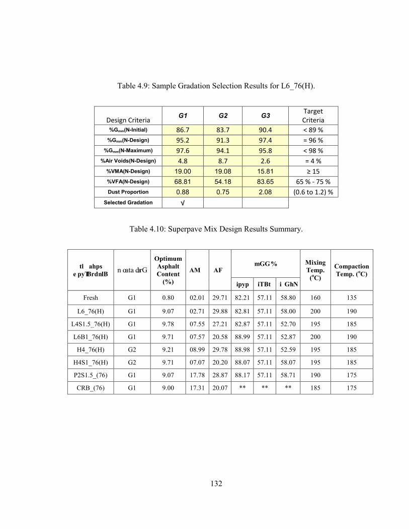
132
Table 4.9: Sample Gradation Selection Results for L6_76(H).
Design Criteria G1 G2 G3 Target
Criteria %Gmm(N-Initial) 86.7 83.7 90.4 < 89 %
%Gmm(N-Design) 95.2 91.3 97.4 = 96 % %Gmm(N-Maximum) 97.6 94.1 95.8 < 98 %
%Air Voids(N-Design) 4.8 8.7 2.6 = 4 % %VMA(N-Design) 19.00 19.08 15.81 ≥ 15 %VFA(N-Design) 68.81 54.18 83.65 65 % - 75 % Dust Proportion 0.88 0.75 2.08 (0.6 to 1.2) %
Selected Gradation √
Table 4.10: Superpave Mix Design Results Summary.
tl ahps e pyTBr dnlB n oata darG
Optimum Asphalt Content
(%)
AM AF %mGG Mixing
Temp. (oC)
Compaction Temp. (oC)
ipyp iTBt i GhN
Fresh G1 0.80 02.01 29.71 82.21 57.11 58.80 160 135
L6_76(H) G1 9.07 02.71 29.88 82.81 57.11 58.00 200 190
L4S1.5_76(H) G1 9.78 07.55 27.21 82.87 57.11 52.70 195 185
L6B1_76(H) G1 9.71 07.57 20.58 88.99 57.11 52.87 200 190
H4_76(H) G2 9.21 08.99 29.78 88.98 57.11 52.59 195 185
H4S1_76(H) G2 9.71 07.07 20.20 88.07 57.11 58.07 195 185
P2S1.5_(76) G1 9.07 17.78 28.87 88.17 57.11 58.71 190 175
CRB_(76) G1 9.00 17.31 20.07 ** ** ** 185 175
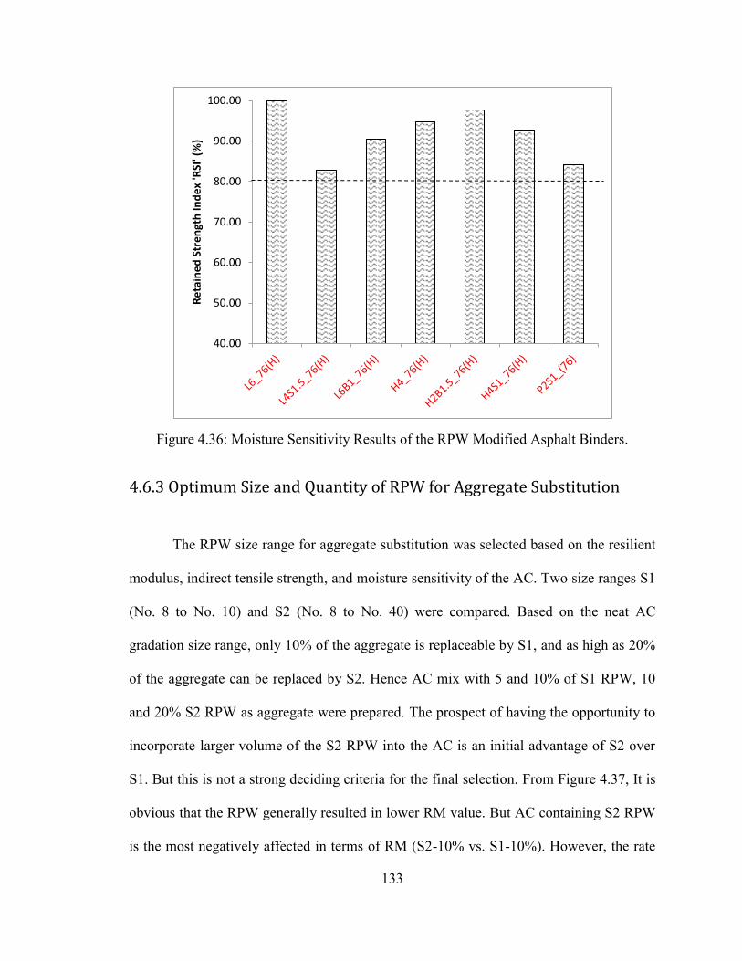
133
Figure 4.36: Moisture Sensitivity Results of the RPW Modified Asphalt Binders.
4.6.3 Optimum Size and Quantity of RPW for Aggregate Substitution
The RPW size range for aggregate substitution was selected based on the resilient
modulus, indirect tensile strength, and moisture sensitivity of the AC. Two size ranges S1
(No. 8 to No. 10) and S2 (No. 8 to No. 40) were compared. Based on the neat AC
gradation size range, only 10% of the aggregate is replaceable by S1, and as high as 20%
of the aggregate can be replaced by S2. Hence AC mix with 5 and 10% of S1 RPW, 10
and 20% S2 RPW as aggregate were prepared. The prospect of having the opportunity to
incorporate larger volume of the S2 RPW into the AC is an initial advantage of S2 over
S1. But this is not a strong deciding criteria for the final selection. From Figure 4.37, It is
obvious that the RPW generally resulted in lower RM value. But AC containing S2 RPW
is the most negatively affected in terms of RM (S2-10% vs. S1-10%). However, the rate
40.00
50.00
60.00
70.00
80.00
90.00
100.00
Re
tain
ed
Str
en
gth
Ind
ex
'RSI
' (%
)
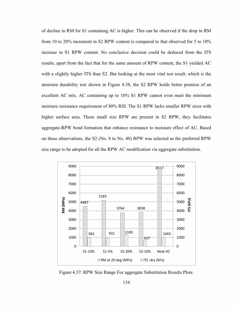
134
of decline in RM for S1 containing AC is higher. This can be observed if the drop in RM
from 10 to 20% increment in S2 RPW content is compared to that observed for 5 to 10%
increase in S1 RPW content. No conclusive decision could be deduced from the ITS
results, apart from the fact that for the same amount of RPW content, the S1 yielded AC
with a slightly higher ITS than S2. But looking at the most vital test result, which is the
moisture durability test shown in Figure 4.38, the S2 RPW holds better promise of an
excellent AC mix. AC containing up to 10% S1 RPW cannot even meet the minimum
moisture resistance requirement of 80% RSI. The S1 RPW lacks smaller RPW sizes with
higher surface area. These small size RPW are present in S2 RPW, they facilitates
aggregate-RPW bond formation that enhance resistance to moisture effect of AC. Based
on these observations, the S2 (No. 8 to No. 40) RPW was selected as the preferred RPW
size range to be adopted for all the RPW AC modification via aggregate substitution.
Figure 4.37: RPW Size Range For aggregate Substitution Results Plots.
4487
5183
3764 3838
8557
965 931 1339
627 1043
0
1000
2000
3000
4000
5000
6000
7000
8000
9000
0
1000
2000
3000
4000
5000
6000
7000
8000
9000
S1-10% S1-5% S2-20% S2-10% Neat AC
ITS
(kP
a)
RM
(M
Pa)
RM at 20 deg (MPa) ITS -dry (kPa)
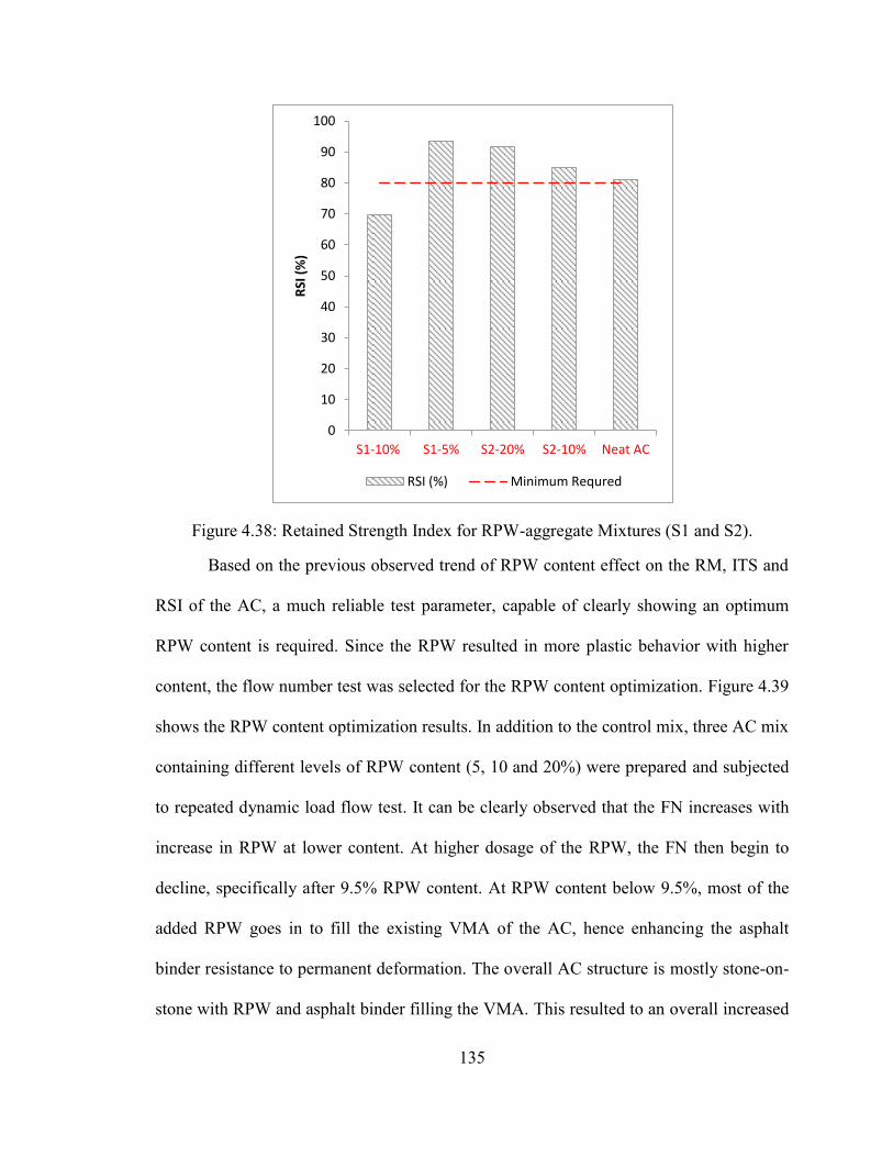
135
Figure 4.38: Retained Strength Index for RPW-aggregate Mixtures (S1 and S2).
Based on the previous observed trend of RPW content effect on the RM, ITS and
RSI of the AC, a much reliable test parameter, capable of clearly showing an optimum
RPW content is required. Since the RPW resulted in more plastic behavior with higher
content, the flow number test was selected for the RPW content optimization. Figure 4.39
shows the RPW content optimization results. In addition to the control mix, three AC mix
containing different levels of RPW content (5, 10 and 20%) were prepared and subjected
to repeated dynamic load flow test. It can be clearly observed that the FN increases with
increase in RPW at lower content. At higher dosage of the RPW, the FN then begin to
decline, specifically after 9.5% RPW content. At RPW content below 9.5%, most of the
added RPW goes in to fill the existing VMA of the AC, hence enhancing the asphalt
binder resistance to permanent deformation. The overall AC structure is mostly stone-on-
stone with RPW and asphalt binder filling the VMA. This resulted to an overall increased
0
10
20
30
40
50
60
70
80
90
100
S1-10% S1-5% S2-20% S2-10% Neat AC
RSI
(%
)
RSI (%) Minimum Requred
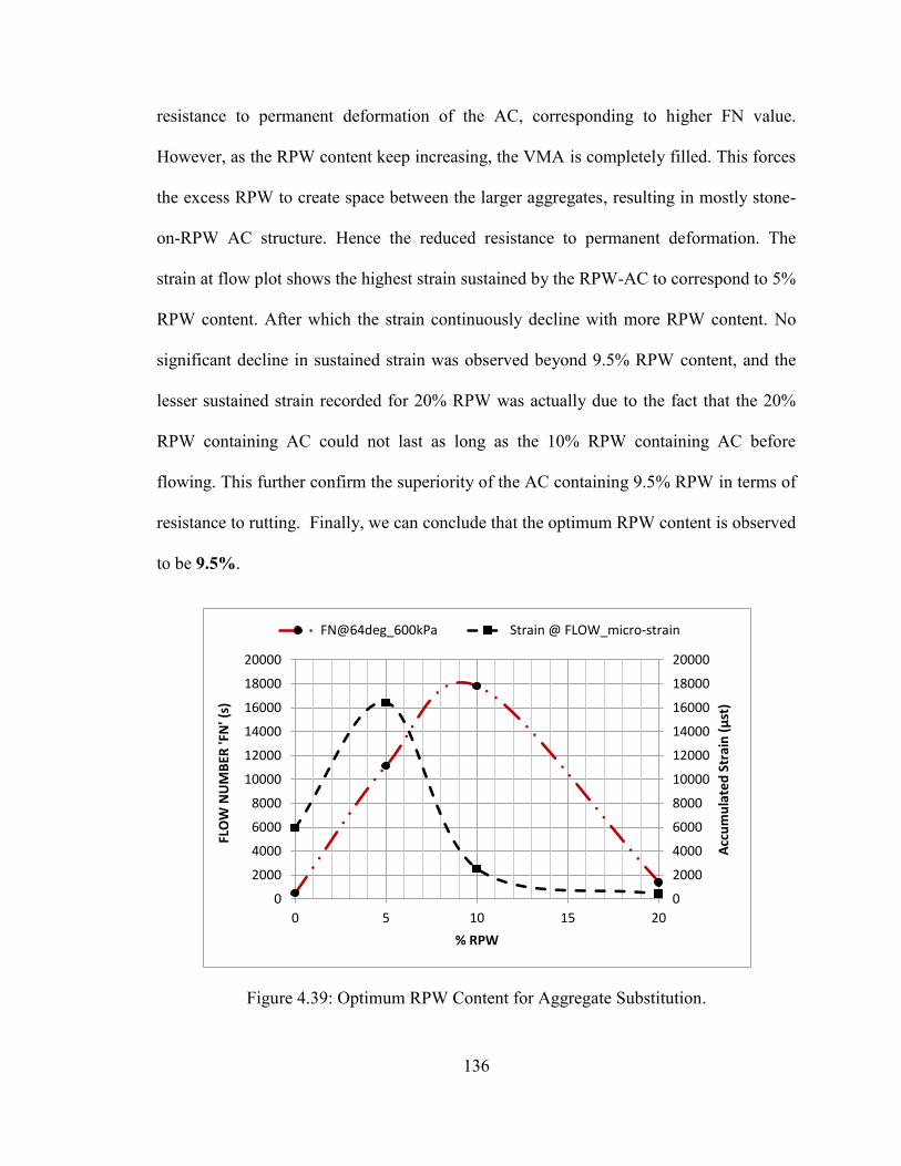
136
resistance to permanent deformation of the AC, corresponding to higher FN value.
However, as the RPW content keep increasing, the VMA is completely filled. This forces
the excess RPW to create space between the larger aggregates, resulting in mostly stone-
on-RPW AC structure. Hence the reduced resistance to permanent deformation. The
strain at flow plot shows the highest strain sustained by the RPW-AC to correspond to 5%
RPW content. After which the strain continuously decline with more RPW content. No
significant decline in sustained strain was observed beyond 9.5% RPW content, and the
lesser sustained strain recorded for 20% RPW was actually due to the fact that the 20%
RPW containing AC could not last as long as the 10% RPW containing AC before
flowing. This further confirm the superiority of the AC containing 9.5% RPW in terms of
resistance to rutting. Finally, we can conclude that the optimum RPW content is observed
to be 9.5%.
Figure 4.39: Optimum RPW Content for Aggregate Substitution.
0
2000
4000
6000
8000
10000
12000
14000
16000
18000
20000
0
2000
4000
6000
8000
10000
12000
14000
16000
18000
20000
0 5 10 15 20
Acc
um
ula
ted
Str
ain
(µ
st)
FLO
W N
UM
BER
'FN
' (s)
% RPW
FN@64deg_600kPa Strain @ FLOW_micro-strain
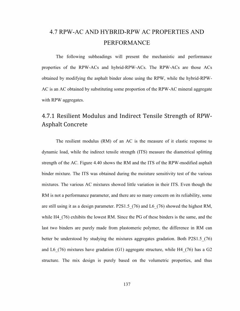
137
4.7 RPW-AC AND HYBRID-RPW AC PROPERTIES AND
PERFORMANCE
The following subheadings will present the mechanistic and performance
properties of the RPW-ACs and hybrid-RPW-ACs. The RPW-ACs are those ACs
obtained by modifying the asphalt binder alone using the RPW, while the hybrid-RPW-
AC is an AC obtained by substituting some proportion of the RPW-AC mineral aggregate
with RPW aggregates.
4.7.1 Resilient Modulus and Indirect Tensile Strength of RPW-
Asphalt Concrete
The resilient modulus (RM) of an AC is the measure of it elastic response to
dynamic load, while the indirect tensile strength (ITS) measure the diametrical splitting
strength of the AC. Figure 4.40 shows the RM and the ITS of the RPW-modified asphalt
binder mixture. The ITS was obtained during the moisture sensitivity test of the various
mixtures. The various AC mixtures showed little variation in their ITS. Even though the
RM is not a performance parameter, and there are so many concern on its reliability, some
are still using it as a design parameter. P2S1.5_(76) and L6_(76) showed the highest RM,
while H4_(76) exhibits the lowest RM. Since the PG of these binders is the same, and the
last two binders are purely made from plastomeric polymer, the difference in RM can
better be understood by studying the mixtures aggregates gradation. Both P2S1.5_(76)
and L6_(76) mixtures have gradation (G1) aggregate structure, while H4_(76) has a G2
structure. The mix design is purely based on the volumetric properties, and thus
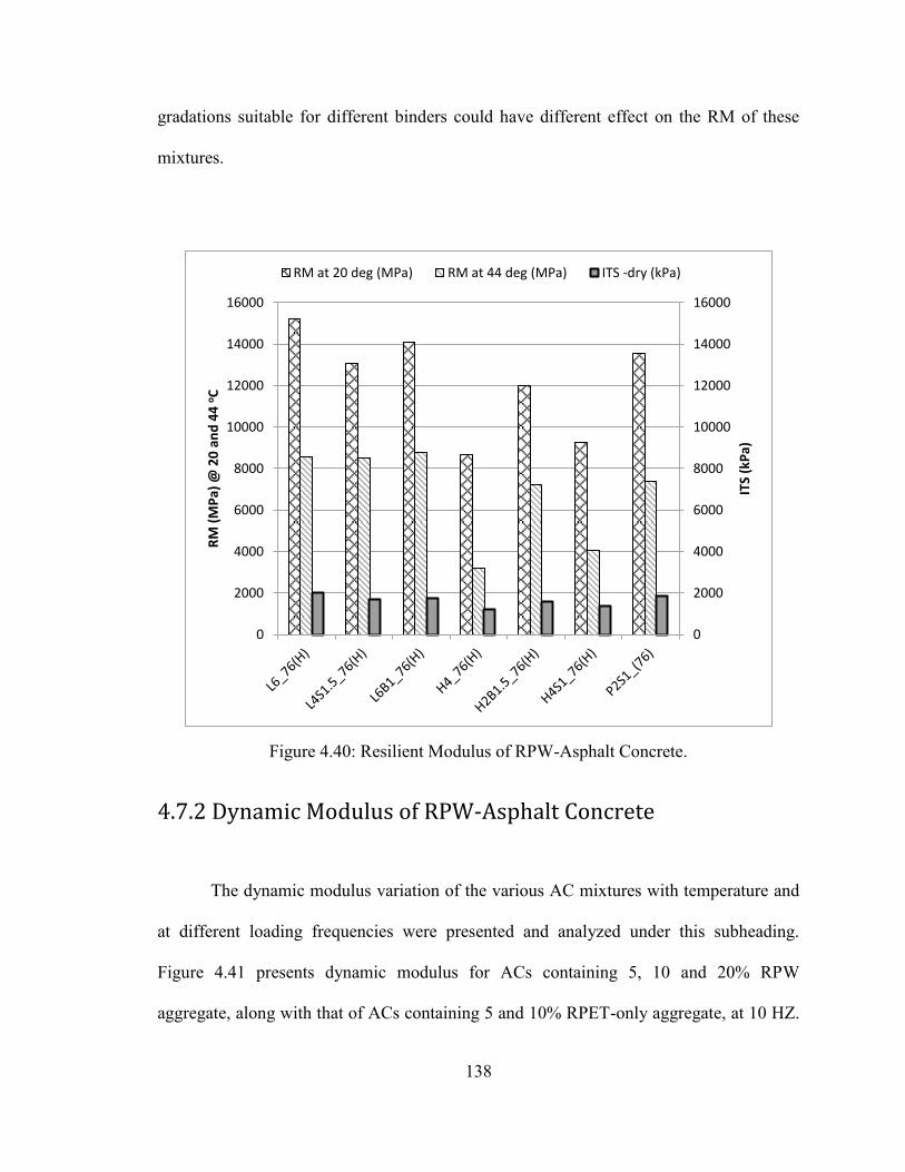
138
gradations suitable for different binders could have different effect on the RM of these
mixtures.
Figure 4.40: Resilient Modulus of RPW-Asphalt Concrete.
4.7.2 Dynamic Modulus of RPW-Asphalt Concrete
The dynamic modulus variation of the various AC mixtures with temperature and
at different loading frequencies were presented and analyzed under this subheading.
Figure 4.41 presents dynamic modulus for ACs containing 5, 10 and 20% RPW
aggregate, along with that of ACs containing 5 and 10% RPET-only aggregate, at 10 HZ.
0
2000
4000
6000
8000
10000
12000
14000
16000
0
2000
4000
6000
8000
10000
12000
14000
16000
ITS
(kP
a)
RM
(M
Pa)
@ 2
0 a
nd
44
oC
RM at 20 deg (MPa) RM at 44 deg (MPa) ITS -dry (kPa)
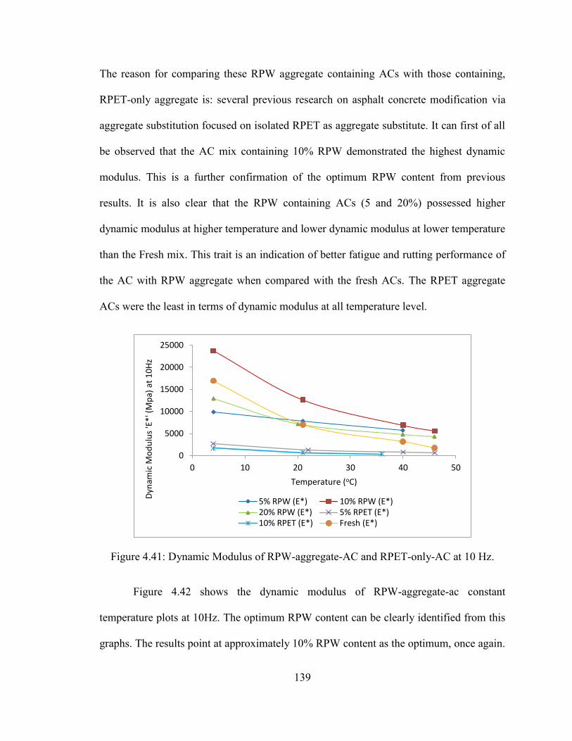
139
The reason for comparing these RPW aggregate containing ACs with those containing,
RPET-only aggregate is: several previous research on asphalt concrete modification via
aggregate substitution focused on isolated RPET as aggregate substitute. It can first of all
be observed that the AC mix containing 10% RPW demonstrated the highest dynamic
modulus. This is a further confirmation of the optimum RPW content from previous
results. It is also clear that the RPW containing ACs (5 and 20%) possessed higher
dynamic modulus at higher temperature and lower dynamic modulus at lower temperature
than the Fresh mix. This trait is an indication of better fatigue and rutting performance of
the AC with RPW aggregate when compared with the fresh ACs. The RPET aggregate
ACs were the least in terms of dynamic modulus at all temperature level.
Figure 4.41: Dynamic Modulus of RPW-aggregate-AC and RPET-only-AC at 10 Hz.
Figure 4.42 shows the dynamic modulus of RPW-aggregate-ac constant
temperature plots at 10Hz. The optimum RPW content can be clearly identified from this
graphs. The results point at approximately 10% RPW content as the optimum, once again.
0
5000
10000
15000
20000
25000
0 10 20 30 40 50
Dyn
amic
Mo
du
lus
'E*'
(M
pa)
at
10
Hz
Temperature (oC)
5% RPW (E*) 10% RPW (E*) 20% RPW (E*) 5% RPET (E*) 10% RPET (E*) Fresh (E*)
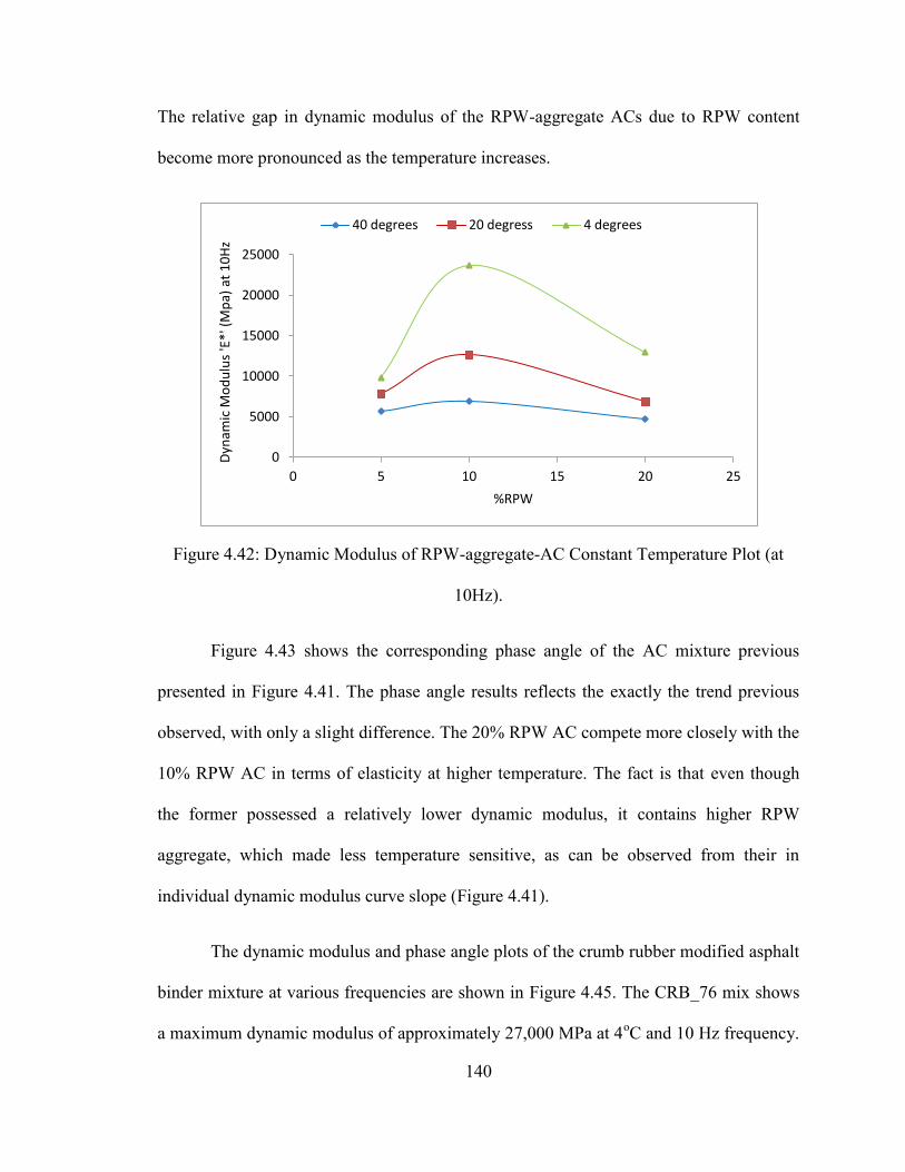
140
The relative gap in dynamic modulus of the RPW-aggregate ACs due to RPW content
become more pronounced as the temperature increases.
Figure 4.42: Dynamic Modulus of RPW-aggregate-AC Constant Temperature Plot (at
10Hz).
Figure 4.43 shows the corresponding phase angle of the AC mixture previous
presented in Figure 4.41. The phase angle results reflects the exactly the trend previous
observed, with only a slight difference. The 20% RPW AC compete more closely with the
10% RPW AC in terms of elasticity at higher temperature. The fact is that even though
the former possessed a relatively lower dynamic modulus, it contains higher RPW
aggregate, which made less temperature sensitive, as can be observed from their in
individual dynamic modulus curve slope (Figure 4.41).
The dynamic modulus and phase angle plots of the crumb rubber modified asphalt
binder mixture at various frequencies are shown in Figure 4.45. The CRB_76 mix shows
a maximum dynamic modulus of approximately 27,000 MPa at 4oC and 10 Hz frequency.
0
5000
10000
15000
20000
25000
0 5 10 15 20 25
Dyn
amic
Mo
du
lus
'E*'
(M
pa)
at
10
Hz
%RPW
40 degrees 20 degress 4 degrees
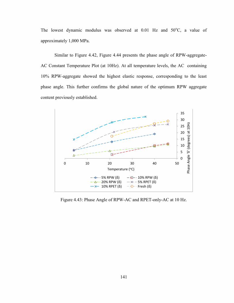
141
The lowest dynamic modulus was observed at 0.01 Hz and 50oC, a value of
approximately 1,000 MPa.
Similar to Figure 4.42, Figure 4.44 presents the phase angle of RPW-aggregate-
AC Constant Temperature Plot (at 10Hz). At all temperature levels, the AC containing
10% RPW-aggregate showed the highest elastic response, corresponding to the least
phase angle. This further confirms the global nature of the optimum RPW aggregate
content previously established.
Figure 4.43: Phase Angle of RPW-AC and RPET-only-AC at 10 Hz.
0
5
10
15
20
25
30
35
0 10 20 30 40 50
Ph
ase
An
gle
'δ' (
deg
rees
) at
10
Hz
Temperature (oC)
5% RPW (δ) 10% RPW (δ) 20% RPW (δ) 5% RPET (δ) 10% RPET (δ) Fresh (δ)
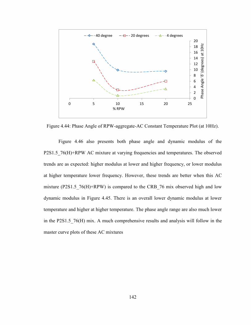
142
Figure 4.44: Phase Angle of RPW-aggregate-AC Constant Temperature Plot (at 10Hz).
Figure 4.46 also presents both phase angle and dynamic modulus of the
P2S1.5_76(H)+RPW AC mixture at varying frequencies and temperatures. The observed
trends are as expected: higher modulus at lower and higher frequency, or lower modulus
at higher temperature lower frequency. However, these trends are better when this AC
mixture (P2S1.5_76(H)+RPW) is compared to the CRB_76 mix observed high and low
dynamic modulus in Figure 4.45. There is an overall lower dynamic modulus at lower
temperature and higher at higher temperature. The phase angle range are also much lower
in the P2S1.5_76(H) mix. A much comprehensive results and analysis will follow in the
master curve plots of these AC mixtures
0
2
4
6
8
10
12
14
16
18
20
0 5 10 15 20 25
Ph
ase
An
gle
'δ' (
deg
rees
) at
10
Hz
% RPW
40 degree 20 degrees 4 degrees
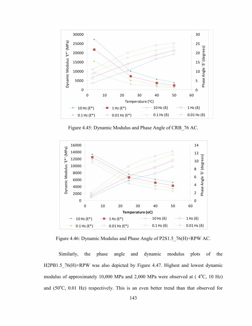
143
Figure 4.45: Dynamic Modulus and Phase Angle of CRB_76 AC.
Figure 4.46: Dynamic Modulus and Phase Angle of P2S1.5_76(H)+RPW AC.
Similarly, the phase angle and dynamic modulus plots of the
H2PB1.5_76(H)+RPW was also depicted by Figure 4.47. Highest and lowest dynamic
modulus of approximately 10,000 MPa and 2,000 MPa were observed at ( 4oC, 10 Hz)
and (50oC, 0.01 Hz) respectively. This is an even better trend than that observed for
0
5000
10000
15000
20000
25000
30000
0 10 20 30 40 50 60
Dyn
amic
Mo
du
lus
'E*
' (M
Pa)
Temperature (oC)
10 Hz (E*) 1 Hz (E*)
0.1 Hz (E*) 0.01 Hz (E*)
0
5
10
15
20
25
30
Ph
ase
An
gle
'δ' (
de
gre
es)
10 Hz (δ) 1 Hz (δ)
0.1 Hz (δ) 0.01 Hz (δ)
0
2000
4000
6000
8000
10000
12000
14000
16000
0 10 20 30 40 50 60
Dyn
amic
Mo
du
lus
'E*
' (M
Pa)
Temperature (oC)
10 Hz (E*) 1 Hz (E*)
0.1 Hz (E*) 0.01 Hz (E*)
0
2
4
6
8
10
12
14
Ph
ase
An
gle
'δ' (
de
gre
es)
10 Hz (δ) 1 Hz (δ)
0.1 Hz (δ) 0.01 Hz (δ)
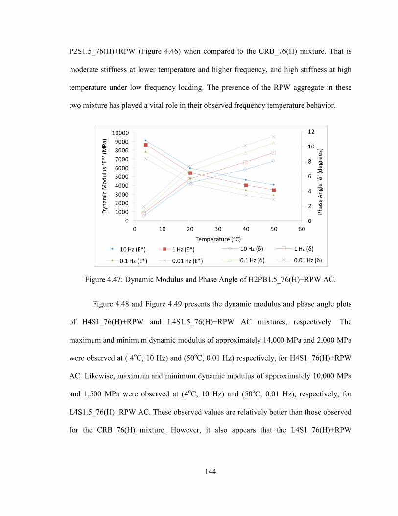
144
P2S1.5_76(H)+RPW (Figure 4.46) when compared to the CRB_76(H) mixture. That is
moderate stiffness at lower temperature and higher frequency, and high stiffness at high
temperature under low frequency loading. The presence of the RPW aggregate in these
two mixture has played a vital role in their observed frequency temperature behavior.
Figure 4.47: Dynamic Modulus and Phase Angle of H2PB1.5_76(H)+RPW AC.
Figure 4.48 and Figure 4.49 presents the dynamic modulus and phase angle plots
of H4S1_76(H)+RPW and L4S1.5_76(H)+RPW AC mixtures, respectively. The
maximum and minimum dynamic modulus of approximately 14,000 MPa and 2,000 MPa
were observed at ( 4oC, 10 Hz) and (50oC, 0.01 Hz) respectively, for H4S1_76(H)+RPW
AC. Likewise, maximum and minimum dynamic modulus of approximately 10,000 MPa
and 1,500 MPa were observed at (4oC, 10 Hz) and (50oC, 0.01 Hz), respectively, for
L4S1.5_76(H)+RPW AC. These observed values are relatively better than those observed
for the CRB_76(H) mixture. However, it also appears that the L4S1_76(H)+RPW
0
1000
2000
3000
4000
5000
6000
7000
8000
9000
10000
0 10 20 30 40 50 60
Dyn
amic
Mo
du
lus
'E*
' (M
Pa)
Temperature (oC)
10 Hz (E*) 1 Hz (E*)
0.1 Hz (E*) 0.01 Hz (E*)
0
2
4
6
8
10
12
Ph
ase
An
gle
'δ' (
de
gre
es)
10 Hz (δ) 1 Hz (δ)
0.1 Hz (δ) 0.01 Hz (δ)
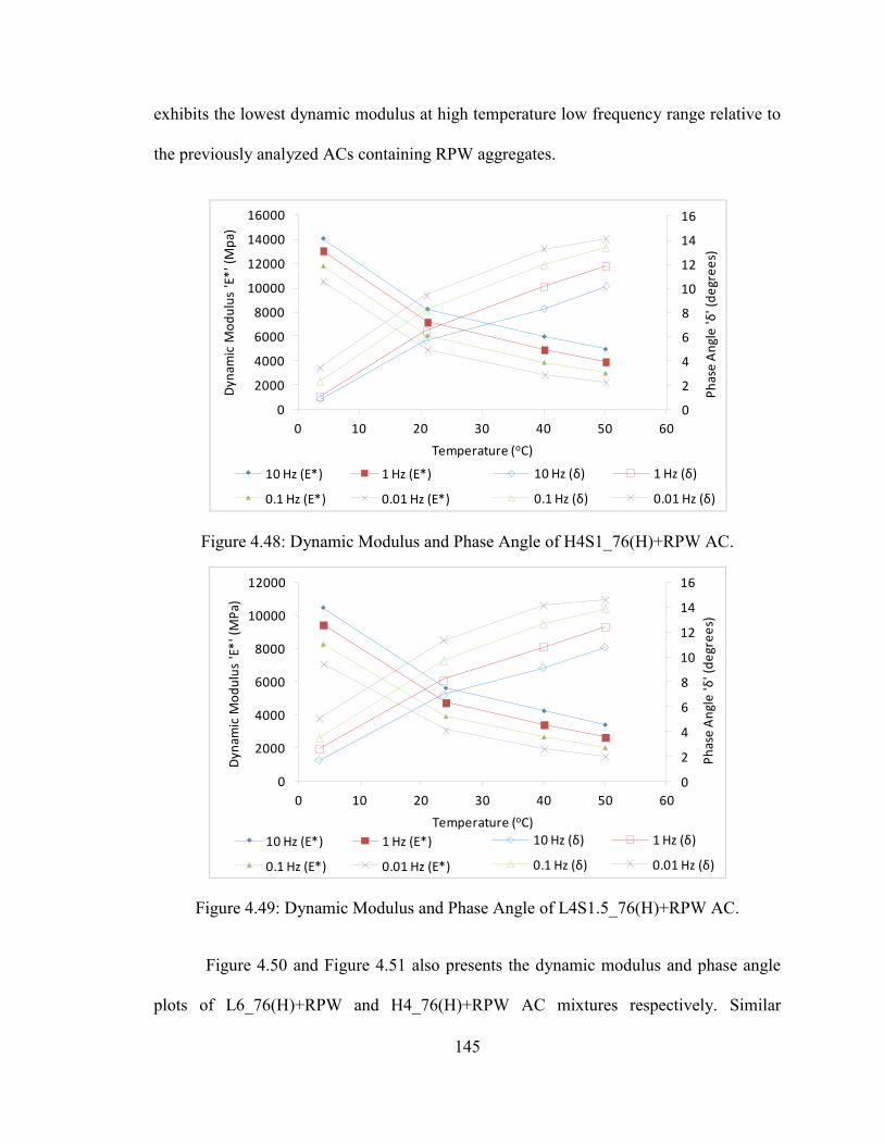
145
exhibits the lowest dynamic modulus at high temperature low frequency range relative to
the previously analyzed ACs containing RPW aggregates.
Figure 4.48: Dynamic Modulus and Phase Angle of H4S1_76(H)+RPW AC.
Figure 4.49: Dynamic Modulus and Phase Angle of L4S1.5_76(H)+RPW AC.
Figure 4.50 and Figure 4.51 also presents the dynamic modulus and phase angle
plots of L6_76(H)+RPW and H4_76(H)+RPW AC mixtures respectively. Similar
0
2000
4000
6000
8000
10000
12000
14000
16000
0 10 20 30 40 50 60
Dyn
amic
Mo
du
lus
'E*
' (M
pa)
Temperature (oC)
10 Hz (E*) 1 Hz (E*)
0.1 Hz (E*) 0.01 Hz (E*)
0
2
4
6
8
10
12
14
16
Ph
ase
An
gle
'δ' (
de
gre
es)
10 Hz (δ) 1 Hz (δ)
0.1 Hz (δ) 0.01 Hz (δ)
0
2000
4000
6000
8000
10000
12000
0 10 20 30 40 50 60
Dyn
amic
Mo
du
lus
'E*
' (M
Pa)
Temperature (oC)
10 Hz (E*) 1 Hz (E*)
0.1 Hz (E*) 0.01 Hz (E*)
0
2
4
6
8
10
12
14
16
Ph
ase
An
gle
'δ' (
de
gre
es)
10 Hz (δ) 1 Hz (δ)
0.1 Hz (δ) 0.01 Hz (δ)
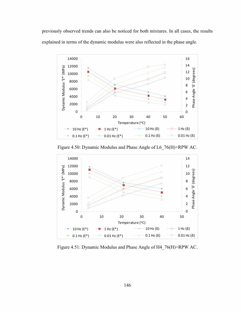
146
previously observed trends can also be noticed for both mixtures. In all cases, the results
explained in terms of the dynamic modulus were also reflected in the phase angle.
Figure 4.50: Dynamic Modulus and Phase Angle of L6_76(H)+RPW AC.
Figure 4.51: Dynamic Modulus and Phase Angle of H4_76(H)+RPW AC.
0
2000
4000
6000
8000
10000
12000
14000
0 10 20 30 40 50 60
Dyn
amic
Mo
du
lus
'E*
' (M
Pa)
Temperature (oC)
10 Hz (E*) 1 Hz (E*)
0.1 Hz (E*) 0.01 Hz (E*)
0
2
4
6
8
10
12
14
16
Ph
ase
An
gle
'δ' (
de
gre
es)
10 Hz (δ) 1 Hz (δ)
0.1 Hz (δ) 0.01 Hz (δ)
0
2000
4000
6000
8000
10000
12000
14000
0 10 20 30 40 50
Dyn
amic
Mo
du
lus
'E*
' (M
Pa)
Temperature (oC)
10 Hz (E*) 1 Hz (E*)
0.1 Hz (E*) 0.01 Hz (E*)
0
2
4
6
8
10
12
14
Ph
ase
An
gle
'δ' (
de
gre
es)
10 Hz (δ) 1 Hz (δ)
0.1 Hz (δ) 0.01 Hz (δ)
147
4.7.2.1 Master Curves of RPW-Asphalt Concrete
The master curve plot for the dynamic modulus of the RPW-ACs was developed
from dynamic modulus results of the asphalt mix performance test. At least 2 replicate
samples are tested at three temperatures within a frequency range of 0.01 to 10 Hz for the
temperature frequency superposition curves [73]. The dynamic modulus was obtained
under a confining stress of 180 kPa, an estimated stress similar to that measured in the
field [74].
Figure 4.52 shows the master curves of the AC mixture containing the combined
RPW aggregate and those containing only RPET aggregate, both compared with fresh
AC. As stated earlier, the reason for RPET-aggregate-only mixture comparison is that for
some reason, most previous research focused on using RPET solely as aggregate
replacement. We have observed that one cannot be able to replace up to 10% of the
aggregate in dense graded mix with RPET without compromising the original superpave
mix design asphalt content. However for the combined RPW (containing all the various
PW), substantial proportion of aggregates could be replaced without losing the binding
ability of the mixture, hence needing no additional asphalt binder. This is due to the
presence of thermoplastic PW in the combined RPW which tend to also serve as binder to
some extent. The thermoplastic PW aggregates tend to partially melt and bind itself to the
mineral aggregates during mixing and compaction period. Since RPET is thermosetting
with high melting temperature in nature, the mixing and compaction temperature did little
to improve bonding between the RPET aggregate and the actual mineral aggregate.
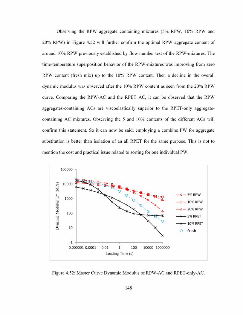
148
Observing the RPW aggregate containing mixtures (5% RPW, 10% RPW and
20% RPW) in Figure 4.52 will further confirm the optimal RPW aggregate content of
around 10% RPW previously established by flow number test of the RPW-mixtures. The
time-temperature superposition behavior of the RPW-mixtures was improving from zero
RPW content (fresh mix) up to the 10% RPW content. Then a decline in the overall
dynamic modulus was observed after the 10% RPW content as seen from the 20% RPW
curve. Comparing the RPW-AC and the RPET AC, it can be observed that the RPW
aggregates-containing ACs are viscoelastically superior to the RPET-only aggregate-
containing AC mixtures. Observing the 5 and 10% contents of the different ACs will
confirm this statement. So it can now be said, employing a combine PW for aggregate
substitution is better than isolation of an all RPET for the same purpose. This is not to
mention the cost and practical issue related to sorting for one individual PW.
Figure 4.52: Master Curve Dynamic Modulus of RPW-AC and RPET-only-AC.
1
10
100
1000
10000
100000
0.000001 0.0001 0.01 1 100 10000 1000000
Dyn
amic
Mod
ulus
'E*'
(MPa
)
Loading Time (s)
5% RPW
10% RPW
20% RPW
5% RPET
10% RPET
Fresh
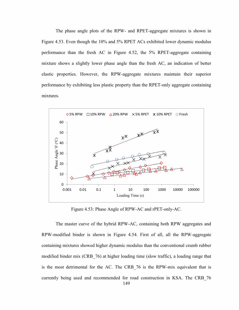
149
The phase angle plots of the RPW- and RPET-aggregate mixtures is shown in
Figure 4.53. Even though the 10% and 5% RPET ACs exhibited lower dynamic modulus
performance than the fresh AC in Figure 4.52, the 5% RPET-aggregate containing
mixture shows a slightly lower phase angle than the fresh AC, an indication of better
elastic properties. However, the RPW-aggregate mixtures maintain their superior
performance by exhibiting less plastic property than the RPET-only aggregate containing
mixtures.
Figure 4.53: Phase Angle of RPW-AC and rPET-only-AC.
The master curve of the hybrid RPW-AC, containing both RPW aggregates and
RPW-modified binder is shown in Figure 4.54. First of all, all the RPW-aggregate
containing mixtures showed higher dynamic modulus than the conventional crumb rubber
modified binder mix (CRB_76) at higher loading time (slow traffic), a loading range that
is the most detrimental for the AC. The CRB_76 is the RPW-mix equivalent that is
currently being used and recommended for road construction in KSA. The CRB_76
0
10
20
30
40
50
60
0.001 0.01 0.1 1 10 100 1000 10000 100000
Phas
e A
ngle
'δ' (
o C)
Loading Time (s)
5% RPW 10% RPW 20% RPW 5% RPET 10% RPET Fresh
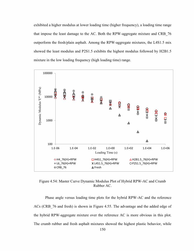
150
exhibited a higher modulus at lower loading time (higher frequency), a loading time range
that impose the least damage to the AC. Both the RPW-aggregate mixture and CRB_76
outperform the fresh/plain asphalt. Among the RPW-aggregate mixtures, the L4S1.5 mix
showed the least modulus and P2S1.5 exhibits the highest modulus followed by H2B1.5
mixture in the low loading frequency (high loading time) range.
Figure 4.54: Master Curve Dynamic Modulus Plot of Hybrid RPW-AC and Crumb Rubber AC.
Phase angle versus loading time plots for the hybrid RPW-AC and the reference
ACs (CRB_76 and fresh) is shown in Figure 4.55. The advantage and the added edge of
the hybrid RPW-aggregate mixture over the reference AC is more obvious in this plot.
The crumb rubber and fresh asphalt mixtures showed the highest plastic behavior, while
100
1000
10000
100000
1.E-06 1.E-04 1.E-02 1.E+00 1.E+02 1.E+04 1.E+06
Dyn
amic
Mod
ulus
'E*'
(MPa
)
Loading Time (s)
H4_76(H)+RPW H4S1_76(H)+RPW H2B1.5_76(H)+RPW
L6_76(H)+RPW L4S1.5_76(H)+RPW P2S1.5_76(H)+RPW
CRB_76 Fresh
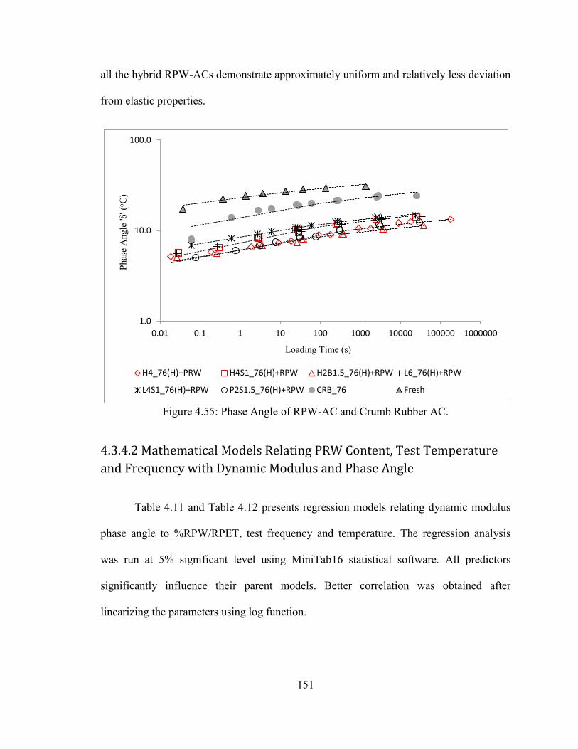
151
all the hybrid RPW-ACs demonstrate approximately uniform and relatively less deviation
from elastic properties.
Figure 4.55: Phase Angle of RPW-AC and Crumb Rubber AC.
4.3.4.2 Mathematical Models Relating PRW Content, Test Temperature
and Frequency with Dynamic Modulus and Phase Angle
Table 4.11 and Table 4.12 presents regression models relating dynamic modulus
phase angle to %RPW/RPET, test frequency and temperature. The regression analysis
was run at 5% significant level using MiniTab16 statistical software. All predictors
significantly influence their parent models. Better correlation was obtained after
linearizing the parameters using log function.
1.0
10.0
100.0
0.01 0.1 1 10 100 1000 10000 100000 1000000
Phas
e A
ngle
'δ' (
o C)
Loading Time (s)
H4_76(H)+PRW H4S1_76(H)+RPW H2B1.5_76(H)+RPW L6_76(H)+RPW
L4S1_76(H)+RPW P2S1.5_76(H)+RPW CRB_76 Fresh
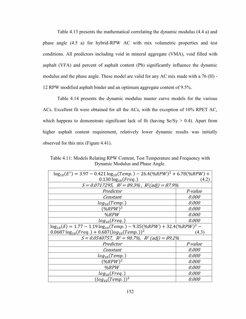
152
Table 4.13 presents the mathematical correlating the dynamic modulus (4.4 a) and
phase angle (4.5 a) for hybrid-RPW AC with mix volumetric properties and test
conditions. All predictors including void in mineral aggregate (VMA), void filled with
asphalt (VFA) and percent of asphalt content (Pb) significantly influence the dynamic
modulus and the phase angle. These model are valid for any AC mix made with a 76 (H) -
12 RPW modified asphalt binder and an optimum aggregate content of 9.5%.
Table 4.14 presents the dynamic modulus master curve models for the various
ACs. Excellent fit were obtained for all the ACs, with the exception of 10% RPET AC,
which happens to demonstrate significant lack of fit (having Se/Sy > 0.4). Apart from
higher asphalt content requirement, relatively lower dynamic results was initially
observed for this mix (Figure 4.41).
Table 4.11: Models Relating RPW Content, Test Temperature and Frequency with Dynamic Modulus and Phase Angle.
(4.2) S = 0.0717295, R2 = 89.3% , R2(adj) = 87.9%
Predictor P-value Constant 0.000
0.000 0.000 0.000
0.000 (4.3)
S = 0.0540757, R2 = 90.7%, R2 (adj) = 89.2% Predictor P-value Constant 0.000
0.000 0.000 0.000
0.000 0.000
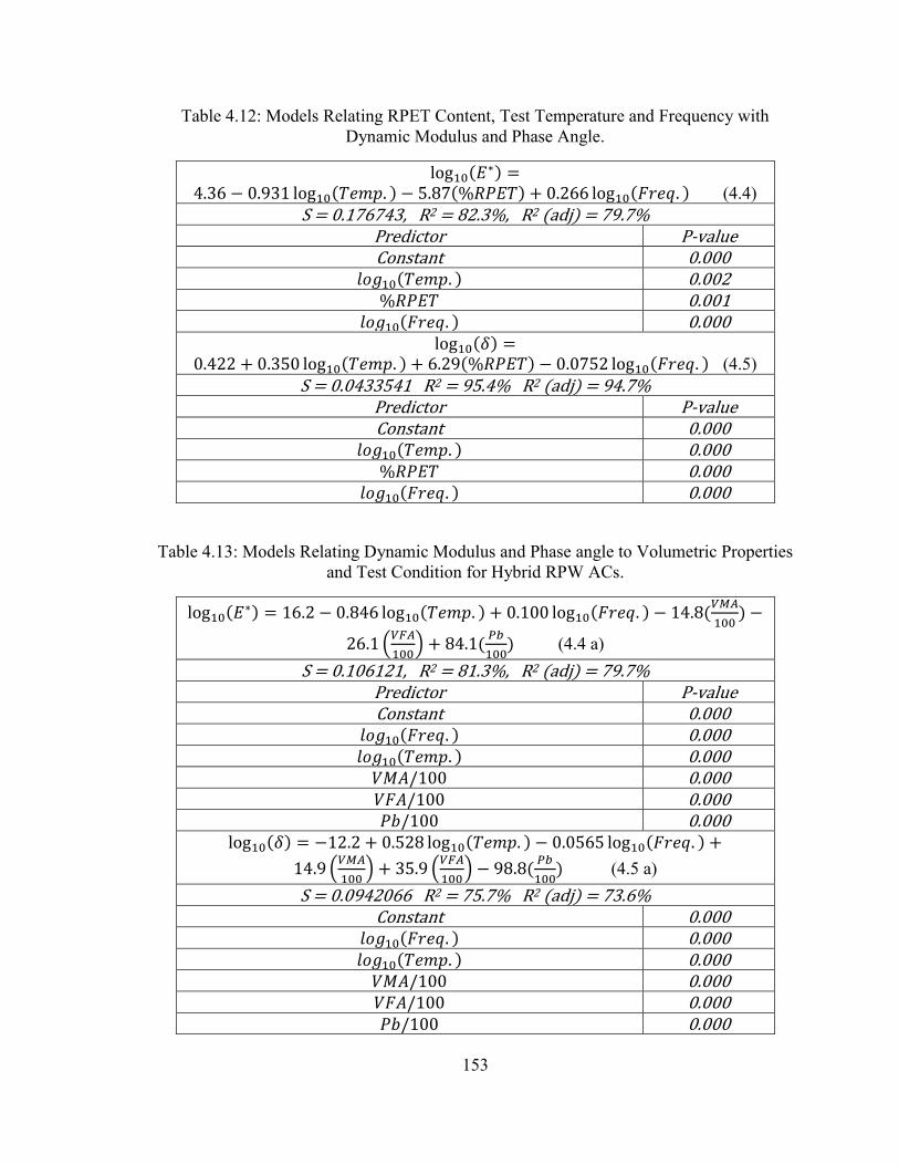
153
Table 4.12: Models Relating RPET Content, Test Temperature and Frequency with Dynamic Modulus and Phase Angle.
(4.4) S = 0.176743, R2 = 82.3%, R2 (adj) = 79.7%
Predictor P-value Constant 0.000
0.002 0.001
0.000
(4.5) S = 0.0433541 R2 = 95.4% R2 (adj) = 94.7%
Predictor P-value Constant 0.000
0.000 0.000
0.000
Table 4.13: Models Relating Dynamic Modulus and Phase angle to Volumetric Properties and Test Condition for Hybrid RPW ACs.
(4.4 a)
S = 0.106121, R2 = 81.3%, R2 (adj) = 79.7% Predictor P-value Constant 0.000
0.000 0.000
0.000 0.000 0.000
(4.5 a)
S = 0.0942066 R2 = 75.7% R2 (adj) = 73.6% Constant 0.000
0.000 0.000
0.000 0.000 0.000
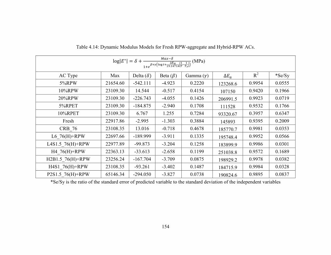
154
Table 4.14: Dynamic Modulus Models for Fresh RPW-aggregate and Hybrid-RPW ACs.
(MPa)
AC Type Max Delta ( Beta ( ) Gamma ( ) R2 *Se/Sy 5%RPW 21654.60 -542.111 -4.923 0.2220 123268.6 0.9954 0.0555 10%RPW 23109.30 14.544 -0.517 0.4154 107150 0.9420 0.1966 20%RPW 23109.30 -226.743 -4.055 0.1426 206991.5 0.9923 0.0719 5%RPET 23109.30 -184.875 -2.940 0.1708 111528 0.9532 0.1766 10%RPET 23109.30 6.767 1.255 0.7284 93320.67 0.3957 0.6347
Fresh 22917.86 -2.995 -1.303 0.3884 145893 0.9395 0.2009 CRB_76 23108.35 13.016 -0.718 0.4678 185770.7 0.9981 0.0353
L6_76(H)+RPW 22697.66 -189.999 -3.911 0.1335 195748.4 0.9952 0.0566 L4S1.5_76(H)+RPW 22977.89 -99.873 -3.204 0.1258 183899.9 0.9986 0.0301
H4_76(H)+RPW 22363.13 -33.613 -2.658 0.1199 251038.8 0.9572 0.1689 H2B1.5_76(H)+RPW 23256.24 -167.704 -3.709 0.0875 198929.2 0.9978 0.0382 H4S1_76(H)+RPW 23108.35 -93.261 -3.402 0.1487 184715.9 0.9984 0.0328
P2S1.5_76(H)+RPW 65146.34 -294.050 -3.827 0.0738 190824.6 0.9895 0.0837 *Se/Sy is the ratio of the standard error of predicted variable to the standard deviation of the independent variables
155
4.7.3 Rutting Performance of RPW-Asphalt Concrete
Two test methods were employed to analyzed the rutting performance of the
RPW-aggregate mixtures, namely: the asphalt pavement analyzer (APA) and the AMPT
flow number test. The APA test method is older and mostly employed specification and
quality assurance, while the AMPT FN test method is more recent and still used for
research and development purpose.
4.7.3.1 Flow Number of RPW-Asphalt Concrete
The FN test results of the various RPW-aggregate-containing AC mixtures and the
reference ACs are shown in Table 4.15. None of the hybrid RWP-aggregate mixture
flowed within the standardized test period of 10,000 seconds. The test was conducted at
the highest operating temperature of the machine (64oC). While the main reference
mixture (CRB_76) shows a relatively very early flow at 1117 seconds. The CRB FN
value falls within the range of AC mixtures eligible for extremely heavy traffic. The FN
test results presented did not disqualify the CRB_76 as an excellent mix, but only shows
an even superior super-performing RPW-aggregate containing AC mixture. Even though
the hybrid RPW-AC did not flow, they have sustained some permanent deformations,
which has been recorded at the end of the test. Comparing these permanent strains of the
hybrid RPW-ACs with that of 4% SBS (another excellent conventional AC mix that did
not flow under similar test condition), will further shows how excellent these mixtures
are. The SBS mix sustained approximately 5000 µst permanent strain at the end of the
test, while most of the hybrid RPW-ACs just about a quarter of this strain.
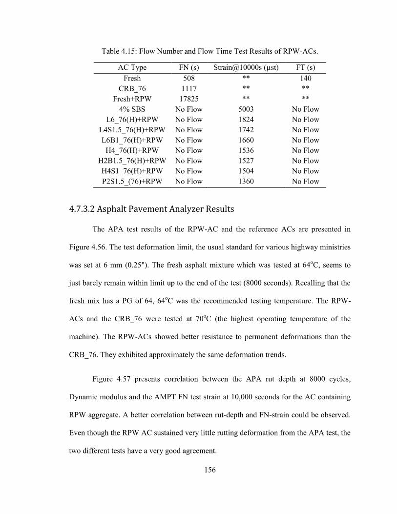
156
Table 4.15: Flow Number and Flow Time Test Results of RPW-ACs.
AC Type FN (s) Strain@10000s (µst) FT (s) Fresh 508 ** 140
CRB_76 1117 ** ** Fresh+RPW 17825 ** **
4% SBS No Flow 5003 No Flow L6_76(H)+RPW No Flow 1824 No Flow
L4S1.5_76(H)+RPW No Flow 1742 No Flow L6B1_76(H)+RPW No Flow 1660 No Flow
H4_76(H)+RPW No Flow 1536 No Flow H2B1.5_76(H)+RPW No Flow 1527 No Flow H4S1_76(H)+RPW No Flow 1504 No Flow P2S1.5_(76)+RPW No Flow 1360 No Flow
4.7.3.2 Asphalt Pavement Analyzer Results
The APA test results of the RPW-AC and the reference ACs are presented in
Figure 4.56. The test deformation limit, the usual standard for various highway ministries
was set at 6 mm (0.25"). The fresh asphalt mixture which was tested at 64oC, seems to
just barely remain within limit up to the end of the test (8000 seconds). Recalling that the
fresh mix has a PG of 64, 64oC was the recommended testing temperature. The RPW-
ACs and the CRB_76 were tested at 70oC (the highest operating temperature of the
machine). The RPW-ACs showed better resistance to permanent deformations than the
CRB_76. They exhibited approximately the same deformation trends.
Figure 4.57 presents correlation between the APA rut depth at 8000 cycles,
Dynamic modulus and the AMPT FN test strain at 10,000 seconds for the AC containing
RPW aggregate. A better correlation between rut-depth and FN-strain could be observed.
Even though the RPW AC sustained very little rutting deformation from the APA test, the
two different tests have a very good agreement.
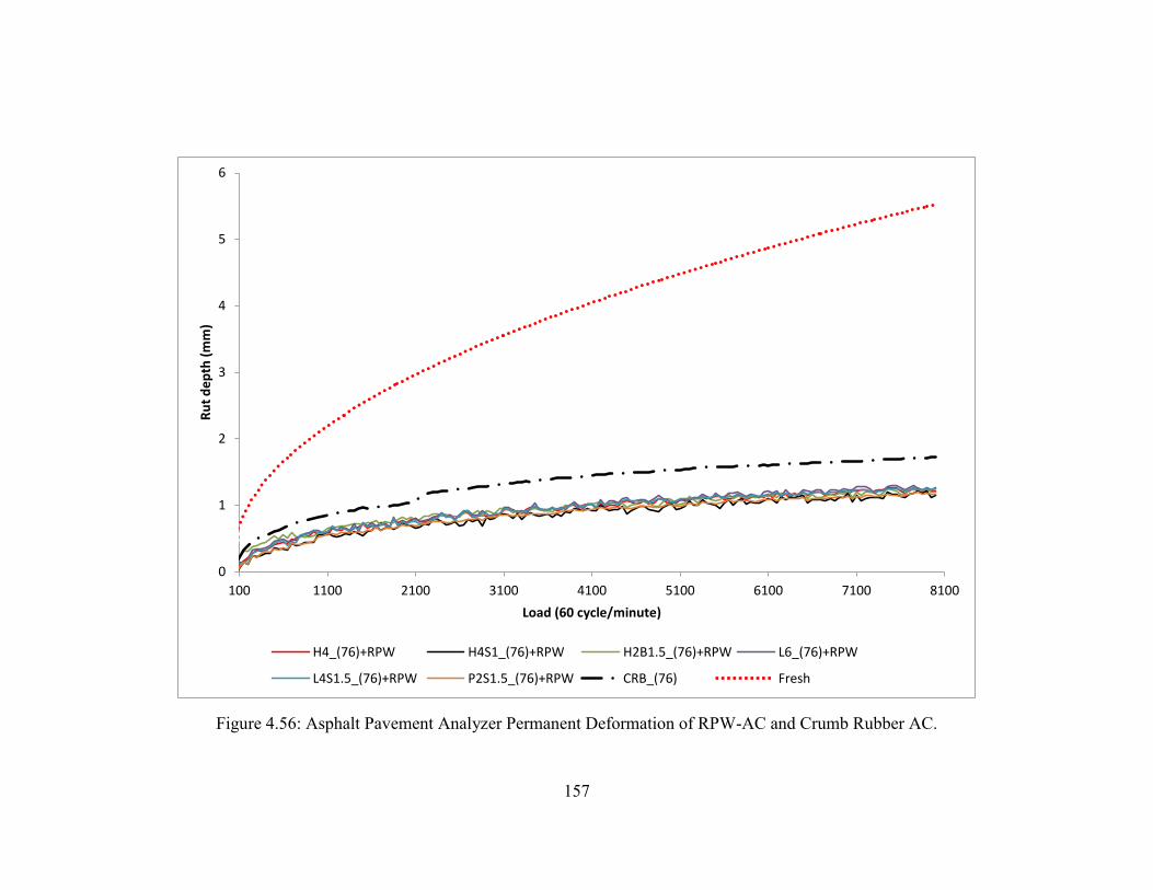
157
Figure 4.56: Asphalt Pavement Analyzer Permanent Deformation of RPW-AC and Crumb Rubber AC.
0
1
2
3
4
5
6
100 1100 2100 3100 4100 5100 6100 7100 8100
Ru
t d
ep
th (
mm
)
Load (60 cycle/minute)
H4_(76)+RPW H4S1_(76)+RPW H2B1.5_(76)+RPW L6_(76)+RPW
L4S1.5_(76)+RPW P2S1.5_(76)+RPW CRB_(76) Fresh
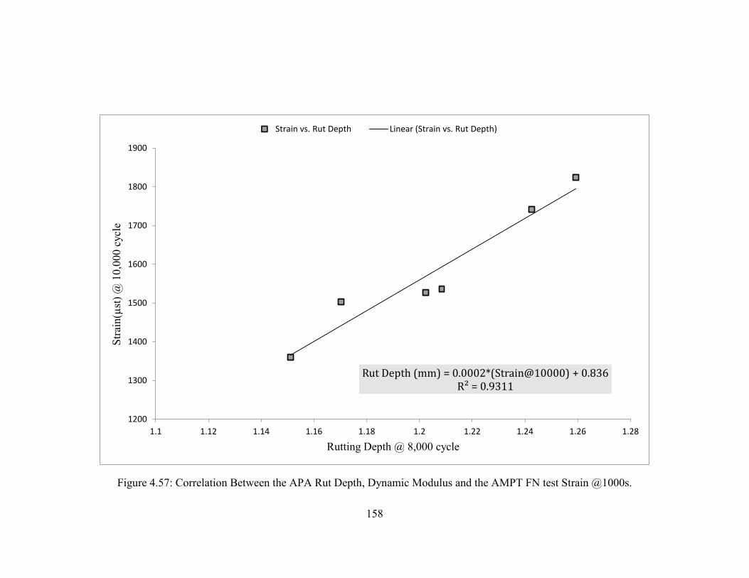
158
Figure 4.57: Correlation Between the APA Rut Depth, Dynamic Modulus and the AMPT FN test Strain @1000s.
Rut Depth (mm) = 0.0002*(Strain@10000) + 0.836 R² = 0.9311
1200
1300
1400
1500
1600
1700
1800
1900
1.1 1.12 1.14 1.16 1.18 1.2 1.22 1.24 1.26 1.28
Stra
in(µ
st) @
10,
000
cycl
e
Rutting Depth @ 8,000 cycle
Strain vs. Rut Depth Linear (Strain vs. Rut Depth)
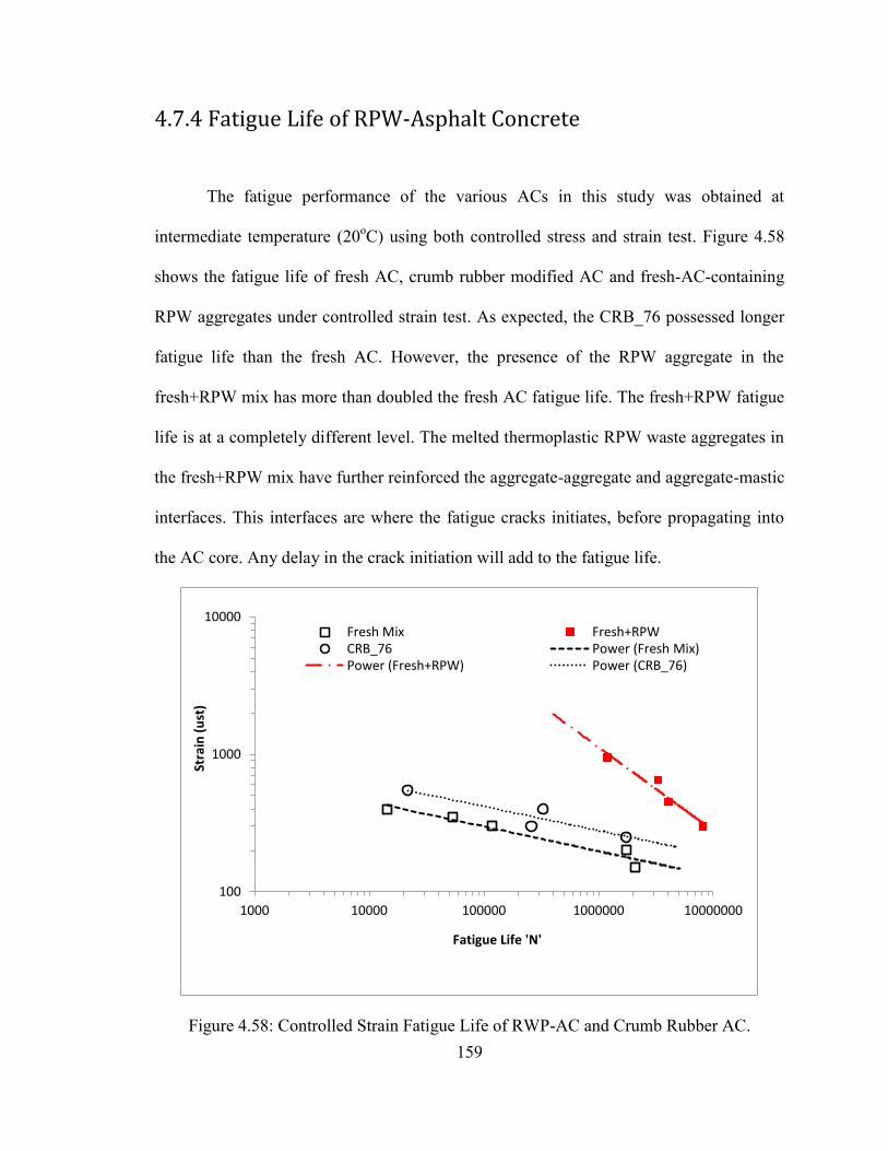
159
4.7.4 Fatigue Life of RPW-Asphalt Concrete
The fatigue performance of the various ACs in this study was obtained at
intermediate temperature (20oC) using both controlled stress and strain test. Figure 4.58
shows the fatigue life of fresh AC, crumb rubber modified AC and fresh-AC-containing
RPW aggregates under controlled strain test. As expected, the CRB_76 possessed longer
fatigue life than the fresh AC. However, the presence of the RPW aggregate in the
fresh+RPW mix has more than doubled the fresh AC fatigue life. The fresh+RPW fatigue
life is at a completely different level. The melted thermoplastic RPW waste aggregates in
the fresh+RPW mix have further reinforced the aggregate-aggregate and aggregate-mastic
interfaces. This interfaces are where the fatigue cracks initiates, before propagating into
the AC core. Any delay in the crack initiation will add to the fatigue life.
Figure 4.58: Controlled Strain Fatigue Life of RWP-AC and Crumb Rubber AC.
100
1000
10000
1000 10000 100000 1000000 10000000
Stra
in (
ust
)
Fatigue Life 'N'
Fresh Mix Fresh+RPW CRB_76 Power (Fresh Mix) Power (Fresh+RPW) Power (CRB_76)
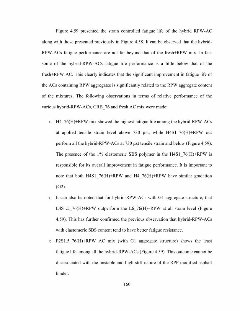
160
Figure 4.59 presented the strain controlled fatigue life of the hybrid RPW-AC
along with those presented previously in Figure 4.58. It can be observed that the hybrid-
RPW-ACs fatigue performance are not far beyond that of the fresh+RPW mix. In fact
some of the hybrid-RPW-ACs fatigue life performance is a little below that of the
fresh+RPW AC. This clearly indicates that the significant improvement in fatigue life of
the ACs containing RPW aggregates is significantly related to the RPW aggregate content
of the mixtures. The following observations in terms of relative performance of the
various hybrid-RPW-ACs, CRB_76 and fresh AC mix were made:
o H4_76(H)+RPW mix showed the highest fatigue life among the hybrid-RPW-ACs
at applied tensile strain level above 730 µst, while H4S1_76(H)+RPW out
perform all the hybrid-RPW-ACs at 730 µst tensile strain and below (Figure 4.59).
The presence of the 1% elastomeric SBS polymer in the H4S1_76(H)+RPW is
responsible for its overall improvement in fatigue performance. It is important to
note that both H4S1_76(H)+RPW and H4_76(H)+RPW have similar gradation
(G2).
o It can also be noted that for hybrid-RPW-ACs with G1 aggregate structure, that
L4S1.5_76(H)+RPW outperform the L6_76(H)+RPW at all strain level (Figure
4.59). This has further confirmed the previous observation that hybrid-RPW-ACs
with elastomeric SBS content tend to have better fatigue resistance.
o P2S1.5_76(H)+RPW AC mix (with G1 aggregate structure) shows the least
fatigue life among all the hybrid-RPW-ACs (Figure 4.59). This outcome cannot be
disassociated with the unstable and high stiff nature of the RPP modified asphalt
binder.
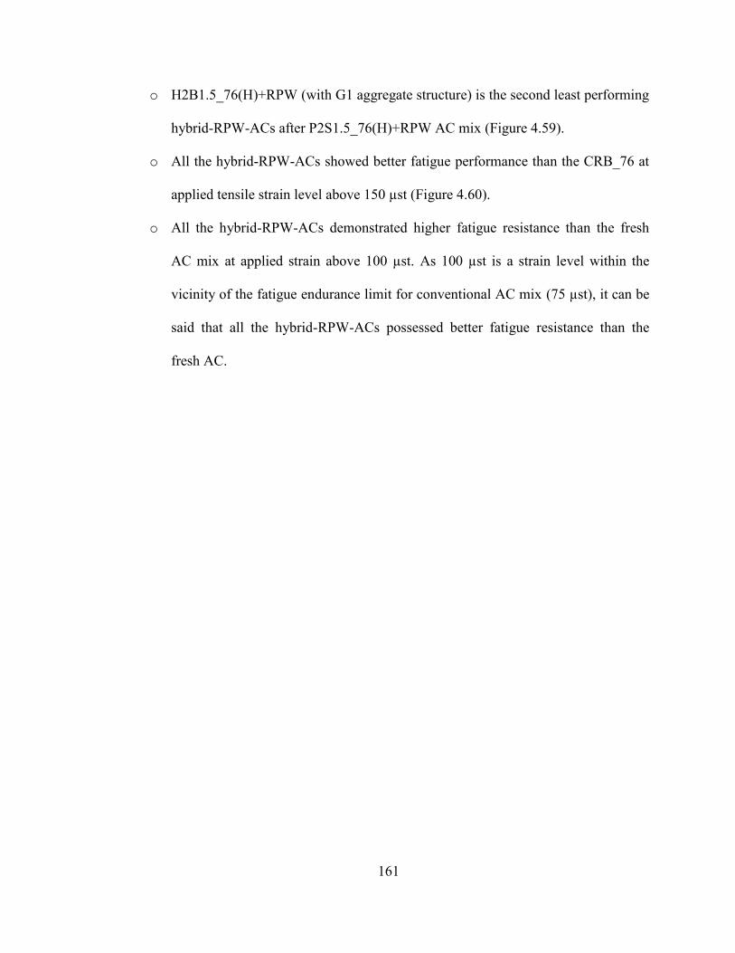
161
o H2B1.5_76(H)+RPW (with G1 aggregate structure) is the second least performing
hybrid-RPW-ACs after P2S1.5_76(H)+RPW AC mix (Figure 4.59).
o All the hybrid-RPW-ACs showed better fatigue performance than the CRB_76 at
applied tensile strain level above 150 µst (Figure 4.60).
o All the hybrid-RPW-ACs demonstrated higher fatigue resistance than the fresh
AC mix at applied strain above 100 µst. As 100 µst is a strain level within the
vicinity of the fatigue endurance limit for conventional AC mix (75 µst), it can be
said that all the hybrid-RPW-ACs possessed better fatigue resistance than the
fresh AC.
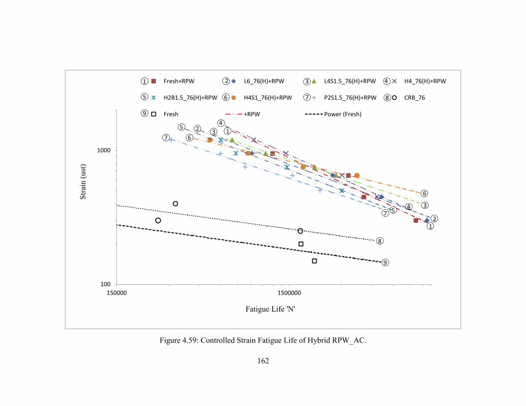
162
Figure 4.59: Controlled Strain Fatigue Life of Hybrid RPW_AC.
100
1000
150000 1500000
Stra
in (u
st)
Fatigue Life 'N'
Fresh+RPW L6_76(H)+RPW L4S1.5_76(H)+RPW H4_76(H)+RPW
H2B1.5_76(H)+RPW H4S1_76(H)+RPW P2S1.5_76(H)+RPW CRB_76
Fresh +RPW Power (Fresh)
1 2 3 4
5 6 7 8
9
7
8
9
6
3
2
6
7 5
1
1 2
3 5
4
4
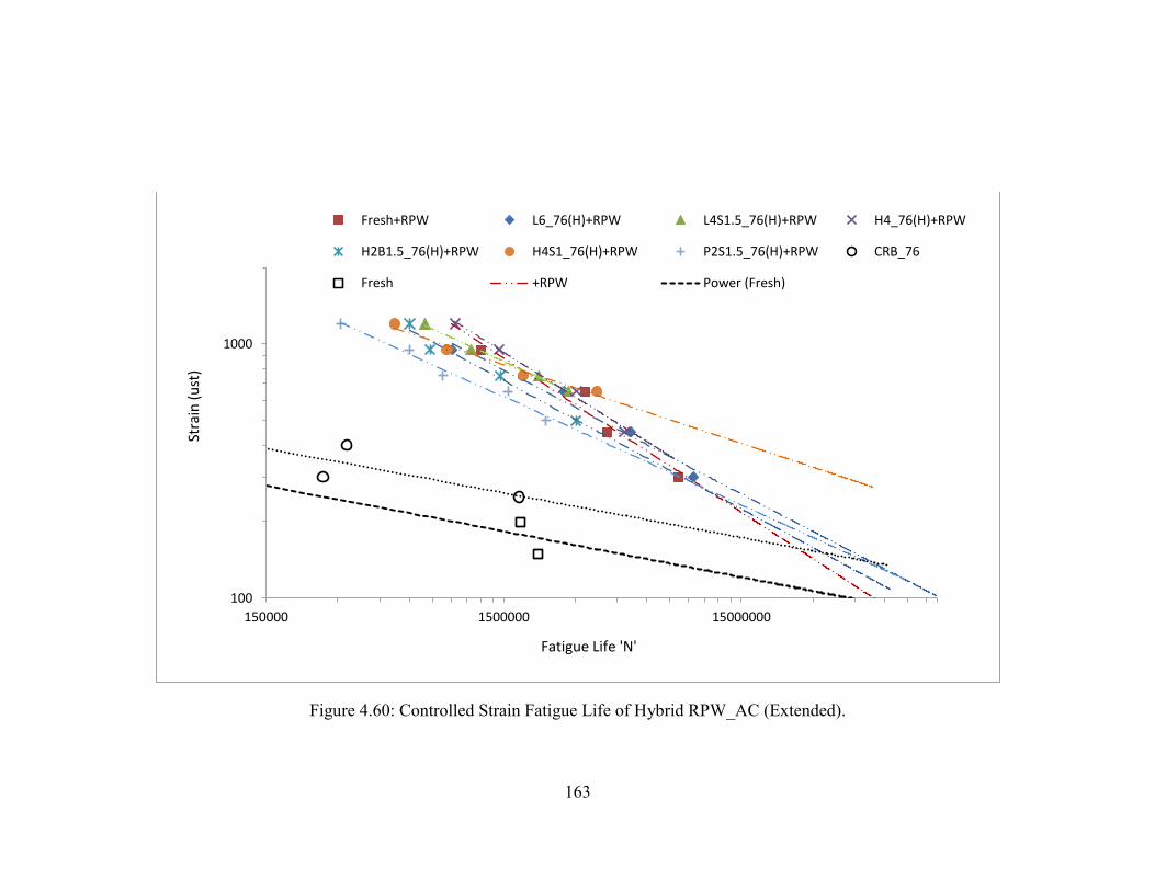
163
Figure 4.60: Controlled Strain Fatigue Life of Hybrid RPW_AC (Extended).
100
1000
150000 1500000 15000000
Stra
in (
ust
)
Fatigue Life 'N'
Fresh+RPW L6_76(H)+RPW L4S1.5_76(H)+RPW H4_76(H)+RPW
H2B1.5_76(H)+RPW H4S1_76(H)+RPW P2S1.5_76(H)+RPW CRB_76
Fresh +RPW Power (Fresh)
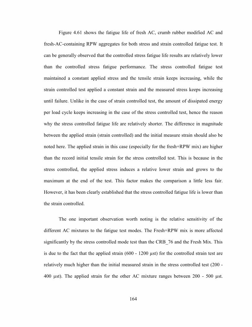
164
Figure 4.61 shows the fatigue life of fresh AC, crumb rubber modified AC and
fresh-AC-containing RPW aggregates for both stress and strain controlled fatigue test. It
can be generally observed that the controlled stress fatigue life results are relatively lower
than the controlled stress fatigue performance. The stress controlled fatigue test
maintained a constant applied stress and the tensile strain keeps increasing, while the
strain controlled test applied a constant strain and the measured stress keeps increasing
until failure. Unlike in the case of strain controlled test, the amount of dissipated energy
per load cycle keeps increasing in the case of the stress controlled test, hence the reason
why the stress controlled fatigue life are relatively shorter. The difference in magnitude
between the applied strain (strain controlled) and the initial measure strain should also be
noted here. The applied strain in this case (especially for the fresh+RPW mix) are higher
than the record initial tensile strain for the stress controlled test. This is because in the
stress controlled, the applied stress induces a relative lower strain and grows to the
maximum at the end of the test. This factor makes the comparison a little less fair.
However, it has been clearly established that the stress controlled fatigue life is lower than
the strain controlled.
The one important observation worth noting is the relative sensitivity of the
different AC mixtures to the fatigue test modes. The Fresh+RPW mix is more affected
significantly by the stress controlled mode test than the CRB_76 and the Fresh Mix. This
is due to the fact that the applied strain (600 - 1200 µst) for the controlled strain test are
relatively much higher than the initial measured strain in the stress controlled test (200 -
400 µst). The applied strain for the other AC mixture ranges between 200 - 500 µst.
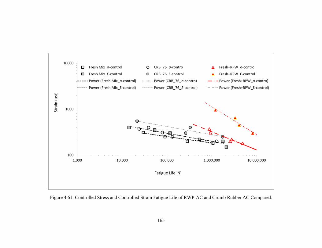
165
Figure 4.61: Controlled Stress and Controlled Strain Fatigue Life of RWP-AC and Crumb Rubber AC Compared.
100
1000
10000
1,000 10,000 100,000 1,000,000 10,000,000
Stra
in (
ust
)
Fatigue Life 'N'
Fresh Mix_σ-control CRB_76_σ-contro Fresh+RPW_σ-contro
Fresh Mix_Ԑ-control CRB_76_Ԑ-control Fresh+RPW_Ԑ-control
Power (Fresh Mix_σ-control) Power (CRB_76_σ-contro) Power (Fresh+RPW_σ-contro)
Power (Fresh Mix_Ԑ-control) Power (CRB_76_Ԑ-control) Power (Fresh+RPW_Ԑ-control)
166
Figure 4.62 presents the controlled stress fatigue life of hybrid-RPW-AC versus
the initial measured applied strain. The same fatigue life result was plotted against the
applied stress as shown in Figure 4.63. The relative performances of the various AC
mixtures is slightly different from the strain controlled test results. Both Figure 4.62 and
Figure 4.63 showed good correlation between the applied load repetition and the fatigue
life. However, the initial strain plot (Figure 4.62) showed a much clearer fatigue life
trend. The following inferences were deduced:
o The CRB_76 AC has better fatigue resistance than the fresh at measured applied
strain above 140 µst, while the Fresh+RPW AC also out-perform the CRB_76 at
strain above 140 µst (Figure 4.62). However, there was intersection between the
CRB_76(H) and Fresh Mix AC fatigue performance curve in the stress versus
load repetition curve (Figure 4.63). It should be noted that these AC mixtures
have similar aggregate gradation, G1.
o All the hybrid-RPW-ACs showed better fatigue resistance than the CRB_76 at
induced strain level above 120 µst (Figure 4.62). However, this measured strain
could possibly correspond to a low applied stress not capable of inducing
cumulative fatigue damage.
o The best performing mix among the hybrid-RPW-ACs is H4S1_76(H) at strain
level below 650 µst. But the Fresh+RPW AC showed better performance above
this strain level.
o As previously observed in the stain controlled test results. The least performing
AC mix among the hybrid-RPW-ACs is the P2S1.5 above 270 µst induced strain.
But H2B1.5_76(H)+RPW showed the least fatigue performance below 270 µst.
167
Figure 4.62: Controlled Stress Fatigue Life of Hybrid RPW_AC (Initial Strain vs. N).
100
1000
10,000 100,000 1,000,000 10,000,000 100,000,000
Initi
al S
train
(ust
)
Fatigue Life 'N'
Fresh Mix CRB_76 Fresh+RPW L6_76(H)+RPW
L4S1.5_76(H)+RPW H4_76(H)+RPW H2B1.5_76(H)+RPW H4S1_76(H)+RPW
P2S1.5_76(H)+RPW Power (Fresh Mix) Power (CRB_76) +RPW
9 1 2
3
8
4 5 6
7
1
1
9
9
8
8 5
5
6
6
3
3
7
7
2
2
4
4
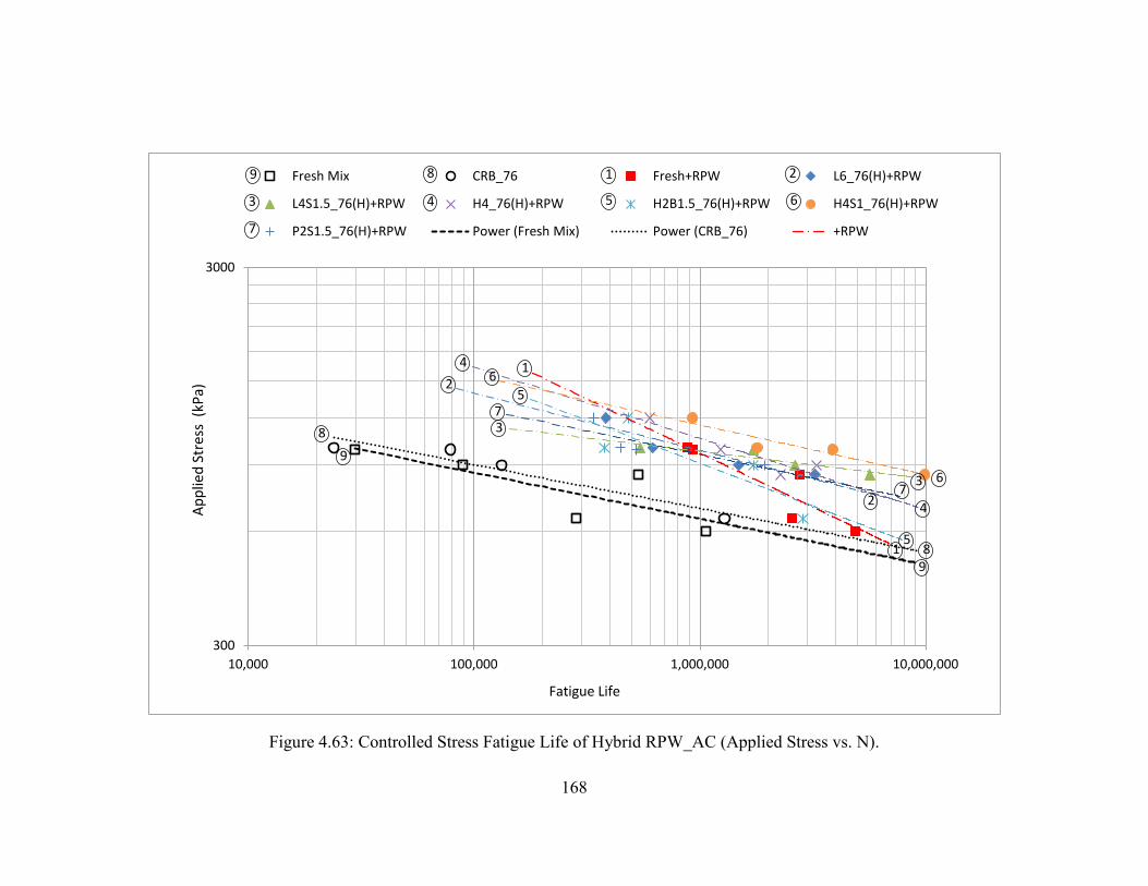
168
Figure 4.63: Controlled Stress Fatigue Life of Hybrid RPW_AC (Applied Stress vs. N).
300
3000
10,000 100,000 1,000,000 10,000,000
Ap
plie
d S
tres
s (
kPa)
Fatigue Life
Fresh Mix CRB_76 Fresh+RPW L6_76(H)+RPW
L4S1.5_76(H)+RPW H4_76(H)+RPW H2B1.5_76(H)+RPW H4S1_76(H)+RPW
P2S1.5_76(H)+RPW Power (Fresh Mix) Power (CRB_76) +RPW
9 8 1 2
3 4 5 6
7
9
9
8
8
1
1
7
7
3
3
6
6
2
2
5
5
4
4
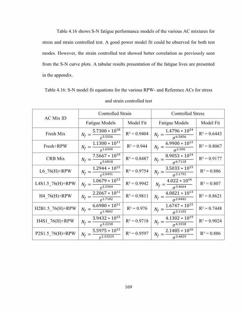
169
Table 4.16 shows S-N fatigue performance models of the various AC mixtures for
stress and strain controlled test. A good power model fit could be observed for both test
modes. However, the strain controlled test showed better correlation as previously seen
from the S-N curve plots. A tabular results presentation of the fatigue lives are presented
in the appendix.
Table 4.16: S-N model fit equations for the various RPW- and Reference ACs for stress
and strain controlled test
AC Mix ID Controlled Strain Controlled Stress
Fatigue Models Model Fit Fatigue Models Model Fit
Fresh Mix
R² = 0.9404
R² = 0.6443
Fresh+RPW
R² = 0.944
R² = 0.8067
CRB Mix
R² = 0.8487
R² = 0.9177
L6_76(H)+RPW
R² = 0.9754
R² = 0.886
L4S1.5_76(H)+RPW
R² = 0.9942
R² = 0.807
H4_76(H)+RPW
R² = 0.9811
R² = 0.8621
H2B1.5_76(H)+RPW
R² = 0.976
R² = 0.7448
H4S1_76(H)+RPW
R² = 0.9718
R² = 0.9024
P2S1.5_76(H)+RPW
R² = 0.9597
R² = 0.886
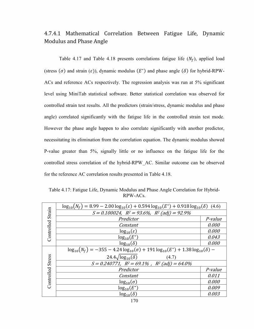
170
4.7.4.1 Mathematical Correlation Between Fatigue Life, Dynamic
Modulus and Phase Angle
Table 4.17 and Table 4.18 presents correlations fatigue life ( ), applied load
(stress and strain ( ), dynamic modulus and phase angle for hybrid-RPW-
ACs and reference ACs respectively. The regression analysis was run at 5% significant
level using MiniTab statistical software. Better statistical correlation was observed for
controlled strain test results. All the predictors (strain/stress, dynamic modulus and phase
angle) correlated significantly with the fatigue life in the controlled strain test mode.
However the phase angle happen to also correlate significantly with another predictor,
necessitating its elimination from the correlation equation. The dynamic modulus showed
P-value greater than 5%, signally little or no influence on the fatigue life for the
controlled stress correlation of the hybrid-RPW_AC. Similar outcome can be observed
for the reference AC correlation results presented in Table 4.18.
Table 4.17: Fatigue Life, Dynamic Modulus and Phase Angle Correlation for Hybrid-RPW-ACs.
Con
trolle
d St
rain
(4.6)
S = 0.100024, R2 = 93.6%, R2 (adj) = 92.9% Predictor P-value Constant 0.000 0.000
0.043 0.000
Con
trolle
d St
ress
(4.7) S = 0.240771, R2 = 69.1% , R2 (adj) = 64.0%
Predictor P-value Constant 0.011 0.000
0.009 0.003
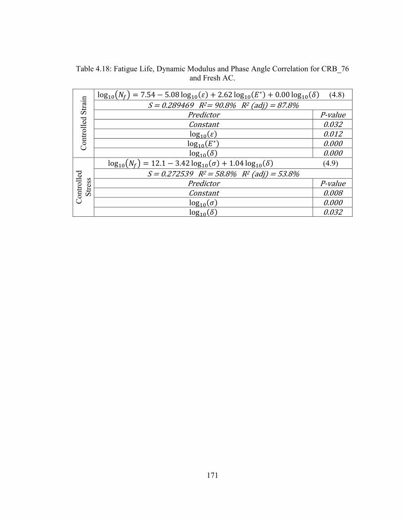
171
Table 4.18: Fatigue Life, Dynamic Modulus and Phase Angle Correlation for CRB_76 and Fresh AC.
Con
trolle
d St
rain
(4.8)
S = 0.289469 R2= 90.8% R2 (adj) = 87.8% Predictor P-value Constant 0.032 0.012
0.000 0.000
Con
trolle
d St
ress
(4.9) S = 0.272539 R2 = 58.8% R2 (adj) = 53.8%
Predictor P-value Constant 0.008 0.000 0.032
172
4.8 RESULTS OF PERFORMANCE MODELING OF RPW-
ASPHALT CONCRETE
The performance modeling of the RPW AC was formulated for the hybrid-RPW
ACs made with RPW-modified binders having upper PG of 76 heavy traffic (30 million
ESAL, Table 3.8). The upper PG of 76 was selected because of the climate requirement in
Eastern Region of KSA. The fatigue and rutting performance of 20 cm hybrid-RPW ACs
wearing course (as shown by Figure 3.24) was modeled. Average seasonal temperature
conditions typical of KSA climate was utilized [78]. All parameters (layer thickness,
traffic loading, climatic data, etc) are kept constant for the hybrid-RPW AC mixtures. The
only property varied is the visco-elastic behavior of the hybrid-RPW AC mixtures.
Average daily equivalent single axle load (ESAL) of 2200, with 5% annual growth was
utilized. A 20 year design period, corresponding to 30 million cumulative ESAL was
used.
4.8.1 Rutting and Fatigue Performance Analysis
The strain induced by the standard axle load in the pavement section (as shown in
Figure 3.24), was obtained using WinJULEA software [76]. WinJulea is a windows
version of the layered elastic program JULEA, which has been implemented in the
AASHTO Mechanistic Empirical Pavement Design Guide for pavements [77]. Using the
standard axle configuration, the critical strain were obtained at the bottom (for fatigue)
and mid section (for rutting) of the AC layer, 20 cm and 10 cm below the surface, directly
under the wheel load. AC layer modulus and Induced strain corresponding to average
173
monthly temperatures were estimated. These parameters were incorporated in to the
rutting and fatigue models (3.41) and (3.45) respectively, for performance prediction.
Figure 4.64 shows the rutting performance results of the hybrid-RPW AC
mixtures relative to fresh and crumb rubber AC mixtures. A handful of the hybrid-RPW
AC mixtures exhibited higher resistance rutting than the CRB_76 and fresh. This trend
was already observed from the master curve laboratory test results. Overall, the hybrid-
RPW AC mixtures did not show any significant rutting throughout the pavements lives.
This has a lot to do with their relatively low temperature sensitivity when compared to the
control and reference mixtures. The RPW aggregates along with the RPW-modified
asphalt binder have lead to ACs with significantly reduced temperature susceptibility.
H4_76(H)+RPW and P2S1_76(H)+RPW showed the highest rutting resistance, while
L4S1.5_76(H)+RPW shows the least resistance to rutting among the hybrid-RPW AC
mixtures. Figure 4.65 shows the correlation between 20 years predicted rutting and
laboratory APA rutting results. Excellent correlation was observed as seen from Figure
4.65.
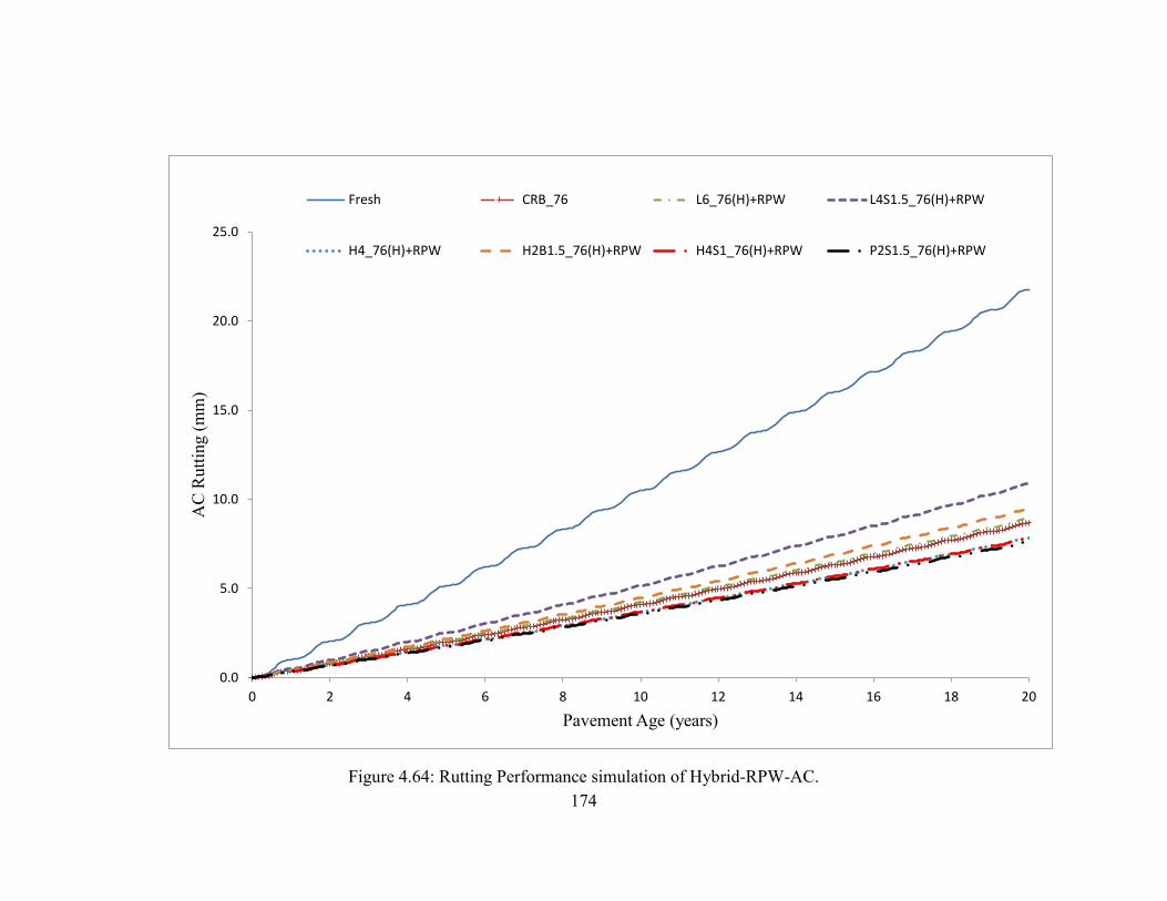
174
Figure 4.64: Rutting Performance simulation of Hybrid-RPW-AC.
0.0
5.0
10.0
15.0
20.0
25.0
0 2 4 6 8 10 12 14 16 18 20
AC
Rut
ting
(mm
)
Pavement Age (years)
Fresh CRB_76 L6_76(H)+RPW L4S1.5_76(H)+RPW
H4_76(H)+RPW H2B1.5_76(H)+RPW H4S1_76(H)+RPW P2S1.5_76(H)+RPW
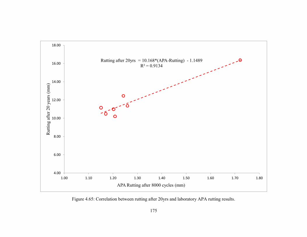
175
Figure 4.65: Correlation between rutting after 20yrs and laboratory APA rutting results.
Rutting after 20yrs = 10.168*(APA-Rutting) - 1.1489 R² = 0.9134
4.00
6.00
8.00
10.00
12.00
14.00
16.00
18.00
1.00 1.10 1.20 1.30 1.40 1.50 1.60 1.70 1.80
Rut
ting
afte
r 20
year
s (m
m)
APA Rutting after 8000 cycles (mm)
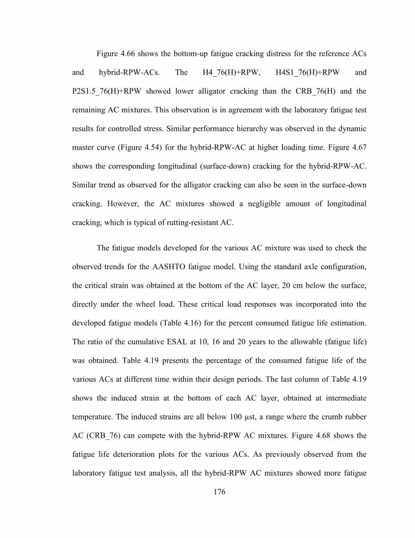
176
Figure 4.66 shows the bottom-up fatigue cracking distress for the reference ACs
and hybrid-RPW-ACs. The H4_76(H)+RPW, H4S1_76(H)+RPW and
P2S1.5_76(H)+RPW showed lower alligator cracking than the CRB_76(H) and the
remaining AC mixtures. This observation is in agreement with the laboratory fatigue test
results for controlled stress. Similar performance hierarchy was observed in the dynamic
master curve (Figure 4.54) for the hybrid-RPW-AC at higher loading time. Figure 4.67
shows the corresponding longitudinal (surface-down) cracking for the hybrid-RPW-AC.
Similar trend as observed for the alligator cracking can also be seen in the surface-down
cracking. However, the AC mixtures showed a negligible amount of longitudinal
cracking, which is typical of rutting-resistant AC.
The fatigue models developed for the various AC mixture was used to check the
observed trends for the AASHTO fatigue model. Using the standard axle configuration,
the critical strain was obtained at the bottom of the AC layer, 20 cm below the surface,
directly under the wheel load. These critical load responses was incorporated into the
developed fatigue models (Table 4.16) for the percent consumed fatigue life estimation.
The ratio of the cumulative ESAL at 10, 16 and 20 years to the allowable (fatigue life)
was obtained. Table 4.19 presents the percentage of the consumed fatigue life of the
various ACs at different time within their design periods. The last column of Table 4.19
shows the induced strain at the bottom of each AC layer, obtained at intermediate
temperature. The induced strains are all below 100 µst, a range where the crumb rubber
AC (CRB_76) can compete with the hybrid-RPW AC mixtures. Figure 4.68 shows the
fatigue life deterioration plots for the various ACs. As previously observed from the
laboratory fatigue test analysis, all the hybrid-RPW AC mixtures showed more fatigue
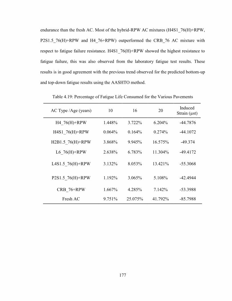
177
endurance than the fresh AC. Most of the hybrid-RPW AC mixtures (H4S1_76(H)+RPW,
P2S1.5_76(H)+RPW and H4_76+RPW) outperformed the CRB_76 AC mixture with
respect to fatigue failure resistance. H4S1_76(H)+RPW showed the highest resistance to
fatigue failure, this was also observed from the laboratory fatigue test results. These
results is in good agreement with the previous trend observed for the predicted bottom-up
and top-down fatigue results using the AASHTO method.
Table 4.19: Percentage of Fatigue Life Consumed for the Various Pavements
AC Type /Age (years) 10 16 20 Induced Strain (µst)
H4_76(H)+RPW 1.448% 3.722% 6.204% -44.7876
H4S1_76(H)+RPW 0.064% 0.164% 0.274% -44.1072
H2B1.5_76(H)+RPW 3.868% 9.945% 16.575% -49.374
L6_76(H)+RPW 2.638% 6.783% 11.304% -49.4172
L4S1.5_76(H)+RPW 3.132% 8.053% 13.421% -55.3068
P2S1.5_76(H)+RPW 1.192% 3.065% 5.108% -42.4944
CRB_76+RPW 1.667% 4.285% 7.142% -53.3988
Fresh AC 9.751% 25.075% 41.792% -85.7988
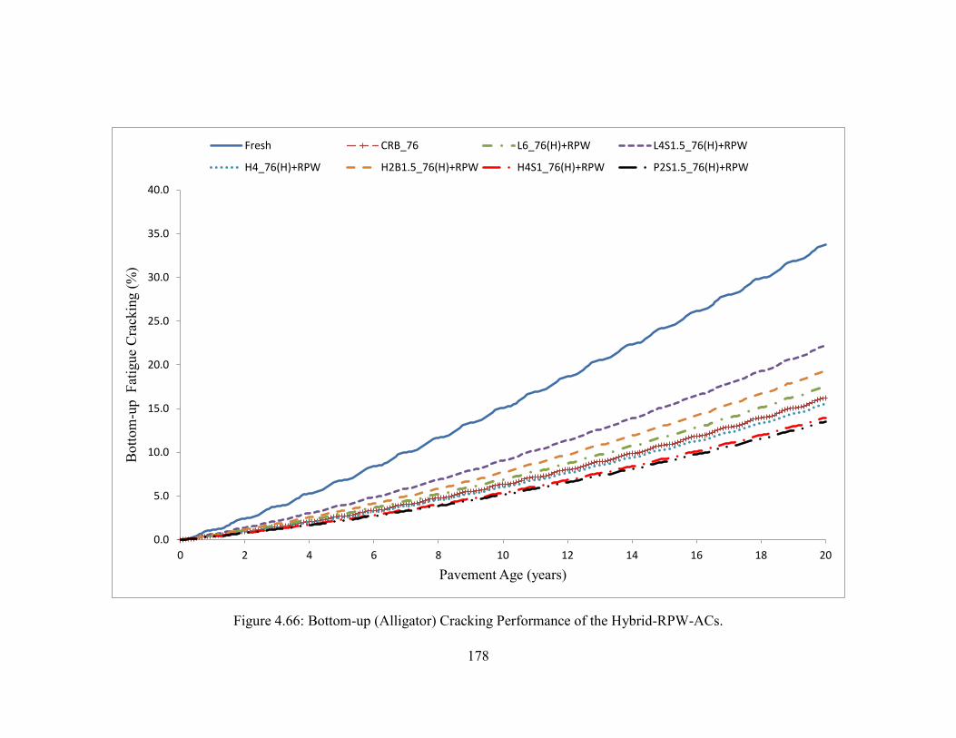
178
Figure 4.66: Bottom-up (Alligator) Cracking Performance of the Hybrid-RPW-ACs.
0.0
5.0
10.0
15.0
20.0
25.0
30.0
35.0
40.0
0 2 4 6 8 10 12 14 16 18 20
Bot
tom
-up
Fat
igue
Cra
ckin
g (%
)
Pavement Age (years)
Fresh CRB_76 L6_76(H)+RPW L4S1.5_76(H)+RPW
H4_76(H)+RPW H2B1.5_76(H)+RPW H4S1_76(H)+RPW P2S1.5_76(H)+RPW
179
Figure 4.67: Surface Down Longitudinal Cracking Performance of the Hybrid-RPW-ACs.
0.0
0.1
0.2
0.3
0.4
0.5
0.6
0.7
0 2 4 6 8 10 12 14 16 18 20
Top-
Dow
n Fa
tigue
Cra
ckin
g (m
/km
)
Pavement Age (years)
Fresh CRB_76 L6_76(H)+RPW L4S1.5_76(H)+RPW
H4_76(H)+RPW H2B1.5_76(H)+RPW H4S1_76(H)+RPW P2S1.5_76(H)+RPW
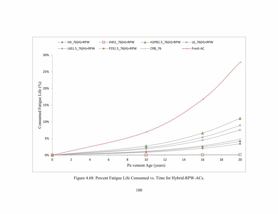
180
Figure 4.68: Percent Fatigue Life Consumed vs. Time for Hybrid-RPW-ACs.
0%
5%
10%
15%
20%
25%
30%
0 2 4 6 8 10 12 14 16 18 20
Con
sum
ed F
atig
ue L
ife (%
)
Pa vement Age (years)
H4_76(H)+RPW H4S1_76(H)+RPW H2PB1.5_76(H)+RPW L6_76(H)+RPW
L4S1.5_76(H)+RPW P2S1.5_76(H)+RPW CRB_76 Fresh AC
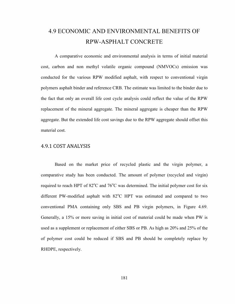
181
4.9 ECONOMIC AND ENVIRONMENTAL BENEFITS OF
RPW-ASPHALT CONCRETE
A comparative economic and environmental analysis in terms of initial material
cost, carbon and non methyl volatile organic compound (NMVOCs) emission was
conducted for the various RPW modified asphalt, with respect to conventional virgin
polymers asphalt binder and reference CRB. The estimate was limited to the binder due to
the fact that only an overall life cost cycle analysis could reflect the value of the RPW
replacement of the mineral aggregate. The mineral aggregate is cheaper than the RPW
aggregate. But the extended life cost savings due to the RPW aggregate should offset this
material cost.
4.9.1 COST ANALYSIS
Based on the market price of recycled plastic and the virgin polymer, a
comparative study has been conducted. The amount of polymer (recycled and virgin)
required to reach HPT of 82oC and 76oC was determined. The initial polymer cost for six
different PW-modified asphalt with 82oC HPT was estimated and compared to two
conventional PMA containing only SBS and PB virgin polymers, in Figure 4.69.
Generally, a 15% or more saving in initial cost of material could be made when PW is
used as a supplement or replacement of either SBS or PB. As high as 20% and 25% of the
of polymer cost could be reduced if SBS and PB should be completely replace by
RHDPE, respectively.
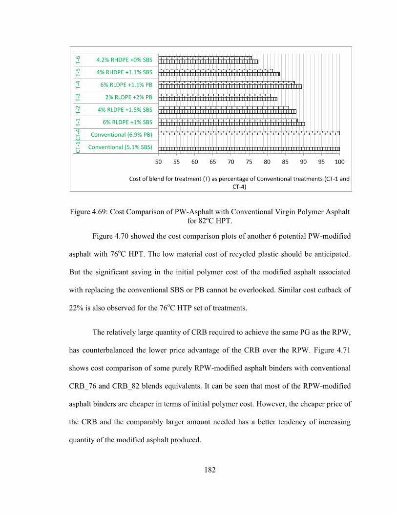
182
Figure 4.69: Cost Comparison of PW-Asphalt with Conventional Virgin Polymer Asphalt for 82ºC HPT.
Figure 4.70 showed the cost comparison plots of another 6 potential PW-modified
asphalt with 76oC HPT. The low material cost of recycled plastic should be anticipated.
But the significant saving in the initial polymer cost of the modified asphalt associated
with replacing the conventional SBS or PB cannot be overlooked. Similar cost cutback of
22% is also observed for the 76oC HTP set of treatments.
The relatively large quantity of CRB required to achieve the same PG as the RPW,
has counterbalanced the lower price advantage of the CRB over the RPW. Figure 4.71
shows cost comparison of some purely RPW-modified asphalt binders with conventional
CRB_76 and CRB_82 blends equivalents. It can be seen that most of the RPW-modified
asphalt binders are cheaper in terms of initial polymer cost. However, the cheaper price of
the CRB and the comparably larger amount needed has a better tendency of increasing
quantity of the modified asphalt produced.
50 55 60 65 70 75 80 85 90 95 100
Conventional (5.1% SBS)
Conventional (6.9% PB)
6% RLDPE +1% SBS
4% RLDPE +1.5% SBS
2% RLDPE +2% PB
6% RLDPE +1.1% PB
4% RHDPE +1.1% SBS
4.2% RHDPE +0% SBS
CT-
1 C
T-4
T-1
T-
2
T-3
T-
4
T-5
T-
6
Cost of blend for treatment (T) as percentage of Conventional treatments (CT-1 and CT-4)
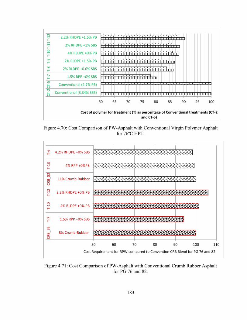
183
Figure 4.70: Cost Comparison of PW-Asphalt with Conventional Virgin Polymer Asphalt for 76ºC HPT.
Figure 4.71: Cost Comparison of PW-Asphalt with Conventional Crumb Rubber Asphalt for PG 76 and 82.
60 65 70 75 80 85 90 95 100
Conventional (3.34% SBS)
Conventional (4.7% PB)
1.5% RPP +0% SBS
2% RLDPE +0.6% SBS
2% RLDPE +1.5% PB
4% RLDPE +0% PB
2% RHDPE +1% SBS
2.2% RHDPE +1.5% PB
CT-
2 C
T-5
T-7
T-
8
T-9
T-1
0 T
-11
T-1
2
Cost of polymer for treatment (T) as percentage of Conventional treatments (CT-2 and CT-5)
50 60 70 80 90 100 110
8% Crumb-Rubber
1.5% RPP +0% SBS
4% RLDPE +0% PB
2.2% RHDPE +0% PB
11% Crumb-Rubber
4% RPP +0%PB
4.2% RHDPE +0% SBS
CR
B_7
6
T-7
T-
10
T-
12
C
RB
_82
T-
13
T-
6
Cost Requirement for RPW compared to Convention CRB Blend for PG 76 and 82
184
4.9.2 ENVIRONMENTAL BENEFITS
Global asphalt demand was estimated at around 120 Million metric tons, with an
annual appreciation forecast of approximately 4% from 2015 [84]. The combined KSA
annual asphalt consumption both from importation and local refineries was estimated at
around 4.6 Million metric tons [85]. Eighty five percent of these asphalt goes in to road
construction, while roofing, waterproofing and other miscellaneous activities consume the
rest [13, 84]. On average [13], six percent polymer equivalent of 80% of the road
construction asphalt is required for the major KSA cities. Which Means, KSA annual
polymer demand for road construction amounts to 187,680 tons, as of 2015. However, the
plastic waste generated each year is more than 7 times the current virgin polymer demand.
Manufacturing a single ton of any commercial polymer from virgin source is
accompanied by major environmental emissions (see Table 3.10). Carbon and NMVOCs
emission are few but critical among the substances emitted during these manufacturing
processes.
Figure 4.72 shows the CO2 and NMVOCs emissions that will results annually if
the selected treatments of PW-asphalt with 82oC HPT and if the incorporated PW were to
be replaced by their exact virgin equivalent, are to be used as asphalt polymer
modification options in KSA. Their equivalent conventional PMA emission results are
also shown. The emission gap between the PW-modified asphalt binder compared to
either the conventional PMA or an exactly virgin polymer equivalent of each treatment is
too wide to ignore. Some of the PW-asphalts have negligible CO2 and NMVOCs
emission. This is the green way, the answer to challenges of the modern construction

185
approaches. Adopting this alternative polymer modification could eliminate up to 500,000
million metric ton of carbon emission and 500 tons of non-methane volatile organic
compounds from our precious atmosphere every year. In general, 27 million metric tons
of carbon emission could be prevented, for each ton of virgin polymer replaced with
recycled one. Similar but relatively lower emission cutbacks could be observed for
treatments with 76oC HPT as shown in Figure 4.73. This is due to fact the quantity of
polymer required to achieve 82oC HPT is higher than that required for 76oC. In all cases,
tremendous amount of CO2 and NMVOCs could be eliminated if the right treatment is
selected.
Figure 4.72: Emission Analogy for Treatments Meeting 82oC HPT.
0 100,000 200,000 300,000 400,000 500,000 600,000
CO2
NMVOCs
CO2
NMVOCs
CO2
NMVOCs
CO2
NMVOCs
CO2
NMVOCs
CO2
NMVOCs
CO2
NMVOCs
CO2
NMVOCs
CT-
1
CT-
4
T-1
T-
2
T-3
T-
4
T-5
T-
6
NMVOCs (kg/Yr), CO2 (MTCO2e/yr)
Conventional PMA Purely Virgin Polymer With Recycled Plastic
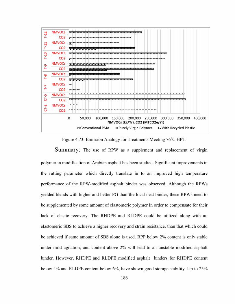
186
Figure 4.73: Emission Analogy for Treatments Meeting 76oC HPT.
Summary: The use of RPW as a supplement and replacement of virgin
polymer in modification of Arabian asphalt has been studied. Significant improvements in
the rutting parameter which directly translate in to an improved high temperature
performance of the RPW-modified asphalt binder was observed. Although the RPWs
yielded blends with higher and better PG than the local neat binder, these RPWs need to
be supplemented by some amount of elastomeric polymer In order to compensate for their
lack of elastic recovery. The RHDPE and RLDPE could be utilized along with an
elastomeric SBS to achieve a higher recovery and strain resistance, than that which could
be achieved if same amount of SBS alone is used. RPP below 2% content is only stable
under mild agitation, and content above 2% will lead to an unstable modified asphalt
binder. However, RHDPE and RLDPE modified asphalt binders for RHDPE content
below 4% and RLDPE content below 6%, have shown good storage stability. Up to 25%
0 50,000 100,000 150,000 200,000 250,000 300,000 350,000 400,000
CO2
NMVOCs
CO2
NMVOCs
CO2
NMVOCs
CO2
NMVOCs
CO2
NMVOCs
CO2
NMVOCs
CO2
NMVOCs
CO2
NMVOCs
CT-
2
CT-
5
T-7
T-
8
T-9
T-
10
T-
11
T-
12
NMVOCs (kg/Yr), CO2 (MTCO2e/Yr)
Conventional PMA Purely Virgin Polymer With Recycled Plastic
187
saving in initial cost of material could be made when PW is used as a supplement or
replacement of virgin polymer. The RPW size ranging between No. 8 to No. 40 was
found to be the best for RPW AC modification via aggregate substitution. The optimum
RPW aggregate content was observed to be 9.5% by weight of the mineral aggregate. The
RPW aggregates-containing ACs are viscoelastically superior to the RPET-only
aggregate-containing AC mixtures. None of the hybrid RWP-aggregate mixture flowed
within the standardized FN test period of 10,000 seconds. The hybrid-RPW ACs have
also showed better resistance to permanent deformations than the CRB_76 when
subjected to repeated wheel load test using the APA. The melted thermoplastic RPW
waste aggregates in the fresh+RPW mix have further reinforced the aggregate-aggregate
and aggregate-mastic interfaces. These interfaces are where the fatigue cracks initiates,
before propagating into the AC core. The delay in the crack initiation has added to the
fatigue life of the fresh+RPW AC. The significant improvement in fatigue life of the
hybrid-RPW ACs is mainly due to the RPW aggregate content of the mixtures. The
simulation results further confirms inferences made from laboratory test results that the
hybrid-RPW ACs are only superior to the CRB_76 AC for higher loading time scenario.
This fact indicates that the hybrid-RPW AC are much suitable to a predominantly hot
climate location.
188
CHAPTER 5
CONCLUSIONS AND RECOMMENDATIONS
This chapter summarizes the conclusive findings from the phases and independent
subheadings of this study. The first subheading presents RPW binder modification
discoveries, where excellent PG and rutting parameters were observed for a relative
cheaper RPW-modified asphalt binder. The major findings on the hybrid RPW-AC
fatigue and rutting performance was summarized in the next following subheading.
Finally the overall findings on the effect of tertiary deformation length on FN, and the
new proposed FN refinement method was presented.
5.1 RPW Modification of Asphalt binder
The use of RPW as a supplement and replacement of virgin polymer in
modification of Arabian asphalt has been studied. Majority of the asphalt RPW-asphalts
demonstrate excellent constructability in terms of high temperature viscosity. Significant
improvements in the rutting parameter which directly translate in to an improved high
temperature performance of the RPW-modified asphalt binder was observed.
Most of the RPWs modified asphalt met the superpave viscosity requirement.
Asphalt blends containing more than 4% RHDPE and in addition to SBS did not meet the
super-pave viscosity criteria. Blends containing more than 6% RLDPE in addition to SBS
failed to pass the viscosity criterion. Eight percent RPP blend containing more than 0.5%
189
SBS, 6% and 4% RPP blend in combination with SBS above 1.5% did not pass the super-
pave viscosity limit criterion
It can be concluded that the upper PG limit increases by almost one level for every
2% increase in the RLDPE or RHDPE content. The improvement of the rutting
performance indicator is more significant in the RHDPE samples than in the RLDPE and
RPP blends. Although the RPWs yielded blends with higher and better PG than the local
neat binder, all the RPWs could not meet the elastic recovery requirement for polymer
modified asphalt binder set by AASHTO TP 70. In order to compensate for their lack of
elastic recovery, these recycled plastic waste need to be supplemented by some amount of
elastomeric polymer.
All the RPWs yields modified asphalt with improved high temperature
performance. Even though the RPWs modified binders lack sufficient strain recovering
ability, RLDPE and RHDPE could be utilized along with an elastomeric SBS to achieve a
higher recovery and strain resistance, than that which could be achieved if same amount
of SBS alone is used. Further investigation into the lower temperature performance of
these RPWs modified asphalt combinations for regions with extremely low temperature
climate is recommended.
RPP below 2% content is only stable under mild agitation, and content above 2%
will lead to an unstable modified asphalt binder. Addition of an elastomeric SBS and
Plastomeric PB minimize the early separation of RPP modified asphalt binder, but does
not necessarily yield stable asphalt binders. As they have shown a potential degrading
tendency with time. RHDPE and RLDPE modified asphalt binders (for RHDPE content
190
below 4% and RLDPE content below 6%) whether containing either SBS or PB have
shown good storage stability trait under mild agitation, both in terms of time degradation
and separation.
All the presented RLDPE-SBS and RLDPE-PB modified asphalts have met 70oC
upper service temperature requirement, a requirement for Medina, Riyadh and Makkah.
Two percent rHDPE is enough to satisfy 70oC high temperature performance requirement
when utilized to modify the Arab asphalt binder. Much adverse high temperature climate
like that of the KSA eastern province requires atleast 3.5% rHDPE modified asphalt
binder to satisfy its high temperature specification. Only Two percent of rPP is required to
yield similar asphalt binder that can endure 76oC high temperature asphalt binder
performance limit.
Up to 25% saving in initial cost of material could be made when PW is used as a
supplement or replacement of virgin polymer. As high as 20 and 22% of the polymer cost
could be reduced, should RHDPE be used as complete replacement. Adopting recycling
alternative of polymer modification in KSA alone could eliminate up to 500,000 million
metric ton of carbon emission and 500 tons of non-methane volatile organic compounds
every year. In general, 27 million metric tons of carbon emission could be prevented, for
each ton of virgin polymer replaced with recycled one.
191
5.2 Rutting and Fatigue Performance of Hybrid RPW-AC
The combined RPW waste from households in Thuqba and Doha, Dhahran KSA
was estimated to approximately consist of 33.7% RPET, 25% RHDPE, 3.8% RPVC,
17.1% RLDPE, 11.6% RPP and 8.8% RPS. This composition was employed for RPW
aggregate in this study.
Based on experimental parameters like RM and ITS, the S2 (No. 8 to No. 40)
RPW appeared to be the best RPW size range, and was adopted for all the RPW AC
modification via aggregate substitution.
According to the observed trend of RPW content effect on the RM, ITS and RSI
of the AC, none of the mentioned test parameter is reliable or capable of clearly showing
an optimum RPW aggregate content. However the FN test has proved adequate in this
regard, and the optimum RPW aggregate content was observed to be 9.5%.
It has been observed that the ACs containing combined RPW aggregates are
viscoelastically superior to the RPET-only aggregate-containing AC mixtures. All the
Hybrid-RPW-ACs showed higher dynamic modulus than the conventional crumb rubber
modified binder mix (CRB_76) at lower loading frequency (slow traffic), a loading time
range that is the most detrimental for the AC. The CRB_76 is the RPW-mix equivalent
that is currently being used and recommended for road construction in KSA. However,
the CRB_76 exhibited a higher modulus at higher loading frequency only, a loading rate
range that imposes the least damage to the AC.
192
None of the hybrid RWP-ACs flowed within the standardized FN test period of
10,000 seconds. While the main reference mixture (CRB_76) shows a relatively very
early flow at 1117 seconds. The hybrid RPW-ACs also showed better resistance to
permanent deformations than the CRB_76 when subjected to repeated wheel load test
using the APA. However, they exhibited approximately the same deformation trends and
all are far away from the deformation limit of 6 mm (within one-third of the limit).
As expected, the CRB_76 possessed longer fatigue life than the fresh AC.
However, the presence of the RPW aggregate in the fresh+RPW mix has more than
doubled the fresh AC fatigue life. The melted thermoplastic RPW waste aggregates in the
fresh+RPW mix have further reinforced the aggregate-aggregate and aggregate-mastic
interfaces. These interfaces are where the fatigue cracks initiate before propagating into
the AC core. The delay in the crack initiation has added to the fatigue life of the
fresh+RPW AC.
The hybrid-RPW-ACs fatigue performance are not far beyond that of the
fresh+RPW mix. In fact of the hybrid-RPW-ACs fatigue life performance is a little below
that of the fresh+RPW AC. This clear indicates that the significant improvement in
fatigue life of the ACs containing RPW aggregates is mainly due to the RPW aggregate
content of the mixtures.
Below are the outline of the major strain controlled fatigue test findings in details:
o H4_76(H)+RPW mix showed the highest fatigue life among the hybrid-
RPW-ACs at applied tensile strain level above 730 µst, while H4S1_76(H)+RPW out
perform all the hybrid-RPW-ACs at 730 µst tensile strain and below. The presence of the
193
1% elastomeric SBS polymer in the H4S1_76(H)+RPW is responsible for its overall
improvement in fatigue performance. It is important to note that both H4S1_76(H)+RPW
and H4_76(H)+RPW have similar gradation (G2).
o It can also be noted that for hybrid-RPW-ACs with G1 aggregate structure,
that L4S1.5_76(H)+RPW outperform the L6_76(H)+RPW at all strain level. This has
further confirmed the previous observation that hybrid-RPW-ACs with elastomeric SBS
content tend to have better fatigue resistance.
o P2S1.5_76(H)+RPW AC mix (with G1 aggregate structure) shows the
least fatigue life among all the hybrid-RPW-ACs. This outcome cannot be disassociated
with the unstable and high stiff nature of the RPP modified asphalt binder.
o H2B1.5_76(H)+RPW (with G1 aggregate structure) is the second least
performing hybrid-RPW-ACs after P2S1.5_76(H)+RPW AC mix.
o All the hybrid-RPW-ACs showed better fatigue performance than the
CRB_76 at applied tensile strain level above 150 µst.
o All the hybrid-RPW-ACs demonstrated higher fatigue resistance than the
fresh AC mix at applied strain above 100 µst. As 100 µst is a strain level within the
vicinity of the fatigue endurance limit for conventional AC mix (75 µst), it can be said
that all the hybrid-RPW-ACs possessed better fatigue resistance than the fresh AC.
Below are the outline of the major stress controlled fatigue test findings in details:
o The CRB_76 AC has better fatigue resistance than the fresh at measured
applied strain above 140 µst, while the Fresh+RPW AC also out-perform the CRB_76 at
strain above 140 µst. However, there was intersection between the CRB_76(H) and Fresh
194
Mix AC fatigue performance curve in the stress versus load repetition curve . It should be
noted that these AC mixtures have similar aggregate gradation, G1.
o All the hybrid-RPW-ACs showed better fatigue resistance than the
CRB_76 at induced strain level above 120 µst. However, this measured strain could
possibly correspond to a low applied stress not capable of inducing cumulative fatigue
damage.
o The best performing mix among the hybrid-RPW-ACs is H4S1_76(H) at
strain level below 650 µst. But the Fresh+RPW AC showed better performance above this
strain level.
o As previously observed in the stain controlled test results. The least
performing AC mix among the hybrid-RPW-ACs is the P2S1.5 above 270 µst induced
strain. But H2B1.5_76(H)+RPW showed the least fatigue performance below 270 µst.
The 20-year simulation results of the RPW modified AC has shown an overall
excellent performance of the RPW modified binder AC mixture, in terms of rutting and
fatigue damage for low intermediate and high temperature climate. It can be concluded
that the RPW modified binder AC mixtures showed satisfactory performance for the
harshest climate in KSA. The simulation results further confirms inferences made from
laboratory test results that most of the hybrid-RPW ACs are superior to the CRB_76 AC
for higher loading time scenario (i.e. high temperature, or slow traffic or both). This
brings us to the conclusion that the hybrid-RPW AC are much suitable to a predominantly
hot climate location.
195
Summary: The lack of elastic recovery on the purely RPW modified binders
was successfully improved by incorporating minor proportion of elastomeric virgin
polymer (SBS). Even though the RPWs modified binders lack sufficient strain recovering
ability, RLDPE and RHDPE could be utilized along with an elastomeric SBS to achieve a
higher recovery and strain resistance, than that which could be achieved if same amount
of SBS alone is employed. Some of the RPP modified asphalt binder (content above 2%)
were found to be unstable. A RPW size ranging between No. 8 and No. 40 was found to
be the best for AC modification via aggregate substitution. An optimum RPW AC
aggregate substitute of 9.5% was established. All the RPW-aggregate containing mixtures
showed higher dynamic modulus than the conventional crumb rubber modified binder
mix (CRB_76) at lower loading frequency. None of the hybrid RWP-aggregate mixture
flowed within the standardized FN test period of 10,000 seconds. The presence of the
RPW aggregate in the fresh+RPW mix has more than doubled the fresh AC fatigue life.
Adopting recycling alternative of polymer modification in KSA alone could eliminate up
to 500,000 million metric tons of carbon emission and 500 tons of non-methane volatile
organic compounds every year. The 20 years simulation results of the RPW modified AC
has shown an overall excellent performance of the RPW modified binder AC mixture.
The simulation results further confirms inferences made from laboratory test results that
the hybrid-RPW ACs are only superior to the CRB_76 AC for higher loading time
scenario (i.e. high temperature, or slow traffic or both). Finally, it is concluded that the
hybrid-RPW AC are much suitable to a predominantly hot climate location.
196
References
1. Zafar, S. Solid Waste Management in Saudi Arabia. EcoMena Articles. 2013;
Available from: http://www.ecomena.org/solid-waste-management-in-saudi-
arabia/.
2. Rahman, F., et al., Catalytic Processing of Waste Plastics With/Without Petroleum
Resid—An Economic Evaluation. Energy Sources, Part A: Recovery, Utilization,
and Environmental Effects, 2006. 28(15): p. 1353-1363.
3. Al-Abdul Wahhab, H.I., et al., Development of performance-based bitumen
specifications for the Gulf countries. Construction and Building Materials, 1997.
11(1): p. 15-22.
4. Ouda, O.K.M. and H.M. Cekirge, Roadmap for Development of Waste-to Energy
Facility in Saudi Arabia. American Journal of Environmental Engineering, 2013.
3(6): p. 6.
5. Huang, Y., R.N. Bird, and O. Heidrich, A review of the use of recycled solid waste
materials in asphalt pavements. Resources, Conservation and Recycling, 2007.
52(1): p. 58-73.
6. Scott, G., ‘Green’ polymers. Polymer Degradation and Stability, 2000. 68(1): p. 1-
7.
7. Thompson, R.C., et al., Plastics, the environment and human health: current
consensus and future trends. Philosophical Transactions of the Royal Society of
London B: Biological Sciences, 2009. 364(1526): p. 2153-2166.
8. Mubaraki, M.A., Predicting Deterioration for the Saudi Arabia Urban Road
Network, in Civil Engineering. 2010, University of Nottingham: Nottingham. p.
271.
197
9. Dalhat, M.A. and H.I. Al-Abdul Wahhab, Performance of Recycled Plastic
Wastes Modified Asphalt binder in Saudi Arabia. International Journal of
Pavement Engineering. DIO: 10.1080/10298436.2015.1088150, 2015.
10. Al-Abdul-Wahhab, H.I., et al. Adaptation Of Shrp Performance Based Binder
Specifications To The Gulf Countries. in Proceedings of the 4th Saudi
Engineering Conference. 1995: KAU.
11. Al-Dubabe, I.A., et al., Polymer Modification of Arab Asphalt. Journal of
Materials in Civil Engineering, 1998. 10(3): p. 161-167.
12. Al-Abdul-Wahhab, H.I., et al., Performance Modification of Saudi Asphalt Binder
Using SABIC Polymer, in Sixth Saudi Engineering Conference. 2002, KFUM:
Dhahran p. 15.
13. Zhu, J., B. Birgisson, and N. Kringos, Polymer modification of bitumen: Advances
and challenges. European Polymer Journal, 2014. 54: p. 18-38.
14. Gourmelon, G., Global Plastic Production Rises, Recycling Lags. 2015, World
Watch Institute: Washington, D.C. p. http://www.worldwatch.org/global-plastic-
production-rises-recycling-lags-0.
15. Wong, S.L., et al., Current state and future prospects of plastic waste as source of
fuel: A review. Renewable and Sustainable Energy Reviews, 2015. 50: p. 1167-
1180.
16. Ouda, O.K.M., et al., Waste-to-energy potential in the Western Province of Saudi
Arabia. Journal of King Saud University - Engineering Sciences, 2015.
http://dx.doi.org/10.1016/j.jksues.2015.02.002.
17. Katami, T., et al., Formation of PCDDs, PCDFs, and Coplanar PCBs from
Polyvinyl Chloride during Combustion in an Incinerator. Environmental Science
& Technology, 2002. 36(6): p. 1320-1324.
198
18. Saikia, N. and J. de Brito, Use of plastic waste as aggregate in cement mortar and
concrete preparation: A review. Construction and Building Materials, 2012. 34: p.
385-401.
19. Siddique, R., J. Khatib, and I. Kaur, Use of recycled plastic in concrete: A review.
Waste Management, 2008. 28(10): p. 1835-1852.
20. Yildirim, Y., Polymer modified asphalt binders. Construction and Building
Materials, 2007. 21(1): p. 66-72.
21. Casey, D., et al., Development of a recycled polymer modified binder for use in
stone mastic asphalt. Resources, Conservation and Recycling, 2008. 52(10): p.
1167-1174.
22. Yildirim, Y., D. Hazlett, and R. Davio, Toner-modified asphalt demonstration
projects. Resources, Conservation and Recycling, 2004. 42(3): p. 295-308.
23. Fang, C., et al., Combined modification of asphalt with polyethylene packaging
waste and organophilic montmorillonite. Polymer Testing, 2012. 31(2): p. 276-
281.
24. Ho, S., et al., Study of recycled polyethylene materials as asphalt modifiers.
Canadian Journal of Civil Engineering, 2006. 33(8): p. 968-981.
25. Murphy, M., et al., Bitumens modified with recycled polymers. Materials and
Structures, 2000. 33(7): p. 438-444.
26. Ahmadinia, E., et al., Performance evaluation of utilization of waste Polyethylene
Terephthalate (PET) in stone mastic asphalt. Construction and Building Materials,
2012. 36(0): p. 984-989.
27. Baghaee Moghaddam, T., M.R. Karim, and T. Syammaun, Dynamic properties of
stone mastic asphalt mixtures containing waste plastic bottles. Construction and
Building Materials, 2012. 34(0): p. 236-242.
199
28. Gandjidoust, H., A. Hassani, and A.A. Maghanaki, Use of plastic waste (poly-
ethylene terephthalate) in asphalt concrete mixture as aggregate replacement.
Waste Management and Research, 2005. 23(4): p. 322+.
29. Zoorob, S.E. and L.B. Suparma, Laboratory design and investigation of the
properties of continuously graded Asphaltic concrete containing recycled plastics
aggregate replacement (Plastiphalt). Cement and Concrete Composites, 2000.
22(4): p. 233-242.
30. Fang, C., et al., UV-Aging Resistance of Packaging Waste PE Modified Asphalts.
Polymer-Plastics Technology and Engineering, 2009. 48(9): p. 945-949.
31. Sangita, et al., Effect of waste polymer modifier on the properties of bituminous
concrete mixes. Construction and Building Materials, 2011. 25(10): p. 3841-3848.
32. García-Morales, M., et al., Linear Viscoelasticity of Recycled EVA-Modified
Bitumens. Energy & Fuels, 2003. 18(2): p. 357-364.
33. Singh, B., M. Gupta, and H. Tarannum, Mastic of polymer-modified bitumen and
poly(vinyl chloride) wastes. Journal of Applied Polymer Science, 2003. 90(5): p.
1347-1356.
34. Fang, C., et al., Modification of waterproofing asphalt by PVC packaging waste.
Journal of Vinyl and Additive Technology, 2009. 15(4): p. 229-233.
35. Navarro, F.J., et al., Bitumen modification with reactive and non-reactive (virgin
and recycled) polymers: A comparative analysis. Journal of Industrial and
Engineering Chemistry, 2009. 15(4): p. 458-464.
36. Punith, V. and A. Veeraragavan, Behavior of Reclaimed Polyethylene Modified
Asphalt Cement for Paving Purposes. Journal of Materials in Civil Engineering,
2011. 23(6): p. 833-845.
37. Fang, C., et al., Aging properties and mechanism of the modified asphalt by
packaging waste polyethylene and waste rubber powder. Polymers for Advanced
Technologies, 2013. 24(1): p. 51-55.
200
38. Singh, B., et al., Polymer-modified bitumen of recycled LDPE and maleated
bitumen. Journal of Applied Polymer Science, 2013. 127(1): p. 67-78.
39. Melbouci, B., S. Sadoun, and A. Bilek, Study of Strengthening of Recycled
Asphalt Concrete by Plastic Aggregates. International Journal of Pavement
Research and Technology, 2014. 7(4): p. 280-286.
40. Gulati, V. (2010) Indian state uses plastic waste for road construction.
http://southasia.oneworld.net/news/indian-state-uses-plastic-waste-for-road-
construction#.WClk3EC7rmQ.
41. Menon, A. (2016) Roads Made of Plastic Waste in India? Yes! Meet the Professor
Who Pioneered the Technique. http://www.thebetterindia.com/43685/plastic-
waste-in-road-construction-plastic-man-india-prof-vasudevan/.
42. Ridden, P. (2012) The streets of Vancouver are paved with ... recycled plastic.
http://newatlas.com/vancouver-recycled-plastic-warm-mix-asphalt/25254/.
43. Lu, X. and U. Isacsson, Compatibility and storage stability of styrene-butadiene-
styrene copolymer modified bitumens. Materials and Structures, 1997. 30(10): p.
618-626.
44. Chen, J.S., M.C. Liao, and C.H. Lin, Determination of polymer content in
modified bitumen. Materials and Structures, 2003. 36(9): p. 594-598.
45. Pérez-Lepe, A., et al., Influence of the processing conditions on the rheological
behaviour of polymer-modified bitumen☆. Fuel, 2003. 82(11): p. 1339-1348.
46. Fu, H., et al., Storage stability and compatibility of asphalt binder modified by
SBS graft copolymer. Construction and Building Materials, 2007. 21(7): p. 1528-
1533.
47. Galooyak, S.S., et al., The Effect of Nanoclay on Rheological Properties and
Storage Stability of SBS-Modified Bitumen. Petroleum Science and Technology,
2011. 29(8): p. 850-859.
201
48. de Carcer, Í.A., et al., Storage stability of SBS/sulfur modified bitumens at high
temperature: Influence of bitumen composition and structure. Construction and
Building Materials, 2014. 52: p. 245-252.
49. Youtcheff, J., N. Wijayatilleke, and A. Shenoy, Evaluation of the Laboratory
Asphalt Stability Test. 2005, Federal Highway Administration. p. FHWA-HRT-
04-111.
50. Li, P., L. Liu, and Z. Sun, Research on the Storage Stability Test Method of SBS
Modified Asphalt, in Proceedings of the 2010 International Conference on
Intelligent Computation Technology and Automation - Volume 03. 2010, IEEE
Computer Society. p. 178-181.
51. Witczak, M., Simple Performance Tests: Summary of Recommended Methods and
Database. 2005, National Cooperative Highway Research Program (NCHRP):
Washinton DC. p. 25.
52. Zhou, F., T. Scullion, and L. Sun, Verification and Modeling of Three-Stage
Permanent Deformation Behavior of Asphalt Mixes. Journal of Transportation
Engineering, 2004. 130(4): p. 486-494.
53. Biligiri, K., et al., Rational Modeling of Tertiary Flow for Asphalt Mixtures.
Journal of the Transportation Research Board, 2007: p. pp. 63–72.
54. Dongré, R., J. D’Angelo, and A. Copeland, Refinement of Flow Number as
Determined by Asphalt Mixture Performance Tester. Journal of the Transportation
Research Board, 2015: p. pp. 127–136.
55. Rodezno, M.C., R. West, and A. Taylor, Flow Number Test and Assessment of
AASHTO TP 79-13 Rutting Criteria. Journal of the Transportation Research
Board, 2015: p. pp. 100–107.
56. Goh, S.W. and Z. You, A simple stepwise method to determine and evaluate the
initiation of tertiary flow for asphalt mixtures under dynamic creep test.
Construction and Building Materials, 2009. 23(11): p. 3398-3405.
202
57. Goh, S., et al., Determination of Flow Number in Asphalt Mixtures from
Deformation Rate During Secondary State. Journal of the Transportation Research
Board, 2011: p. pp, 106–112.
58. Alavi, A.H., et al., Formulation of flow number of asphalt mixes using a hybrid
computational method. Construction and Building Materials, 2011. 25(3): p. 1338-
1355.
59. Yan, K.-z., D.-d. Ge, and Z. Zhang, Support Vector Machine Models for
Prediction of Flow Number of Asphalt Mixtures. Int. J. Pavement Res. Technol,
2014. 7(1): p. 10.
60. Apeagyei, A.K., Flow number predictive models from volumetric and binder
properties. Construction and Building Materials, 2014. 64: p. 240-245.
61. AASHTO:T321, Standard Method of Test for Determining the Fatigue Life of
Compacted Asphalt Mixtures Subjected to Repeated Flexural Bending. 2014,
AASHTO: Washington, DC 20001
62. ASTM:D7460-10, Standard Test Method for Determining Fatigue Failure of
Compacted Asphalt Concrete Subjected to Repeated Flexural Bending. 2010,
ASTM International: West Conshohocken, PA.
63. Tarefder, R.A., D. Bateman, and A.K. Swamy, Comparison of fatigue failure
criterion in flexural fatigue test. International Journal of Fatigue, 2013. 55: p. 213-
219.
64. Qiu, K., et al., Thermo-mechanical coupling effect on fatigue behavior of cement
asphalt mortar. International Journal of Fatigue, 2013. 51: p. 116-120.
65. Al-Khateeb, G.G. and K.A. Ghuzlan, The combined effect of loading frequency,
temperature, and stress level on the fatigue life of asphalt paving mixtures using
the IDT test configuration. International Journal of Fatigue, 2014. 59: p. 254-261.
203
66. Mannan, U.A., M.R. Islam, and R.A. Tarefder, Effects of recycled asphalt
pavements on the fatigue life of asphalt under different strain levels and loading
frequencies. International Journal of Fatigue, 2015. 78: p. 72-80.
67. Pronk, A.C. Comparison of 2 and 4 Point Fatigue Tests and Healing in 4-Point
Dynamic Bending Test Based on the Dissipated Energy Concept. in Eighth
International Conference on Asphalt Pavements 1997. Seattle, Washington.:
Transportation Research Board.
68. Rowe, G.M. and M.G. Bouldin., IMPROVED TECHNIQUES TO EVALUATE
THE FATIGUE RESISTANCE OF ASPHALTIC MIXTURES, in 2nd Eurasphalt &
Eurobitume Congress 2000, Proc.0081.uk: Barcelona.
69. Carpenter, S., K. Ghuzlan, and S. Shen, Fatigue Endurance Limit for Highway
and Airport Pavements. Transportation Research Record: Journal of the
Transportation Research Board, 2003. 1832: p. 131-138.
70. Abojaradeh, M., Effective Fatigue Models for Arizona Asphalt Concrete Mixtures.
PhD Dissertation, in Civil Engineering. 2003, Arizona State University: Tempe,
AZ.
71. AASHTO:M323, Standard Specification for Superpave Volumetric Mix Design.
2013, AASHTO: WASHINTON DC, 2001.
72. AASHTO:TP_79-15, Standard Method of Test for Determining the Dynamic
Modulus and Flow Number for Asphalt Mixtures Using the AMPT, . 2015,
AASHTO.: Washington, DC 20001
73. Bonaquist, R. and D. Christensen, Practical Procedure for Developing Dynamic
Modulus Master Curves for Pavement Structural Design. Transportation Research
Record: Journal of the Transportation Research Board, 2005. 1929: p. 208-217.
74. Hajj, E., et al., Estimation of Stress Conditions for the Flow Number Simple
Performance Test. Transportation Research Record: Journal of the Transportation
Research Board, 2010. 2181: p. 67-78.
204
75. Li, Q., et al., Mechanistic-empirical pavement design guide (MEPDG): a bird’s-
eye view. Journal of Modern Transportation, 2011. 19(2): p. 114-133.
76. Hossain E.I, N., D. Singh, and M. Zaman P.E, Dynamic Modulus-based Field Rut
Prediction Model from an Instrumented Pavement Section. Procedia - Social and
Behavioral Sciences, 2013. 104: p. 129-138.
77. ARA, Guide for the mechanistic empirical design of new and rehabilitated
pavement structures. 2004, Transportation Research Board of the National
Academies: Washington, DC.
78. Wheatherbase, Monthly Wheather Average Summary. 2017, CantyMedia:
Dammam, Saudi Arabia.
79. Ulloa, A., et al., Equivalent Loading Frequencies for Dynamic Analysis of Asphalt
Pavements. Journal of Materials in Civil Engineering, 2013. 25(9): p. 1162-1170.
80. ICIS, ICIS Pricing: Petrochemical, energy and fertilizer market intelligence.
2014, ICIS.
81. EPA, Plastics, OCSPP, Editor. 2010, Environmental Protection Agency: U.S.
82. Kuenen, J., et al., EMEP/EEA emission inventory guidebook, in 2.B Chemical
industry, E.E. Agency, Editor. 2013, EEA: Copenhagen K.
83. Saygın, D., et al., CHEMICAL AND PETROCHEMICAL SECTOR, in Potential of
best practice technology and other measures for improving energy efficiency.
2009, INTERNATIONAL ENERGY AGENCY. p. 60.
84. Freedonia. World Asphalt - Demand and Sales Forecasts, Market Share, Market
Size, Market Leaders. 2014 Study #: 3129]; 429]. Available from:
http://www.freedoniagroup.com/World-Asphalt.html.
85. United-Nation, Energy and Renewables: UN Statistics Division Energy Statistics
Database for Saudi Arabia. 2013, KNOEMA.
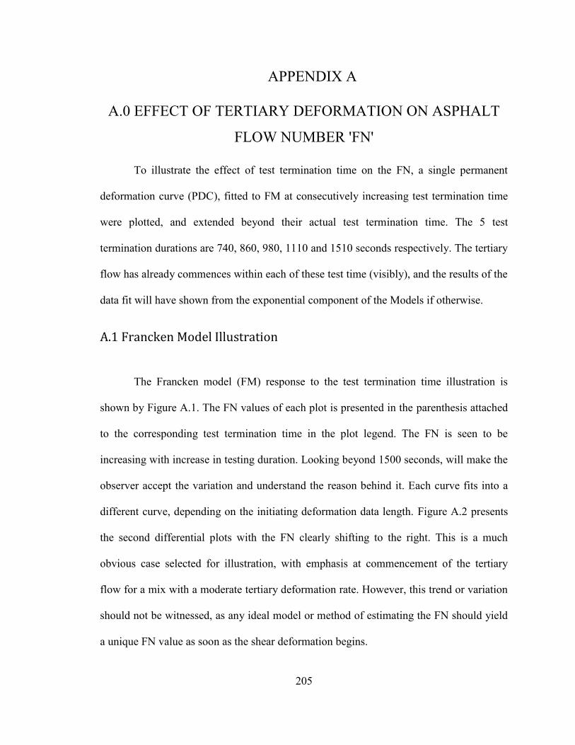
205
A. APPENDIX A
A.0 EFFECT OF TERTIARY DEFORMATION ON ASPHALT
FLOW NUMBER 'FN'
To illustrate the effect of test termination time on the FN, a single permanent
deformation curve (PDC), fitted to FM at consecutively increasing test termination time
were plotted, and extended beyond their actual test termination time. The 5 test
termination durations are 740, 860, 980, 1110 and 1510 seconds respectively. The tertiary
flow has already commences within each of these test time (visibly), and the results of the
data fit will have shown from the exponential component of the Models if otherwise.
A.1 Francken Model Illustration
The Francken model (FM) response to the test termination time illustration is
shown by Figure A.1. The FN values of each plot is presented in the parenthesis attached
to the corresponding test termination time in the plot legend. The FN is seen to be
increasing with increase in testing duration. Looking beyond 1500 seconds, will make the
observer accept the variation and understand the reason behind it. Each curve fits into a
different curve, depending on the initiating deformation data length. Figure A.2 presents
the second differential plots with the FN clearly shifting to the right. This is a much
obvious case selected for illustration, with emphasis at commencement of the tertiary
flow for a mix with a moderate tertiary deformation rate. However, this trend or variation
should not be witnessed, as any ideal model or method of estimating the FN should yield
a unique FN value as soon as the shear deformation begins.
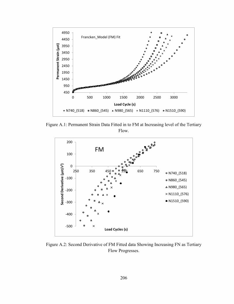
206
Figure A.1: Permanent Strain Data Fitted in to FM at Increasing level of the Tertiary Flow.
Figure A.2: Second Derivative of FM Fitted data Showing Increasing FN as Tertiary Flow Progresses.
450
950
1450
1950
2450
2950
3450
3950
4450
4950
0 500 1000 1500 2000 2500 3000
Pe
rman
en
t St
rain
(µ
st)
Load Cycle (s)
Francken_Model (FM) Fit
N740_(518) N860_(545) N980_(565) N1110_(576) N1510_(590)
-500
-400
-300
-200
-100
0
100
200
250 350 450 550 650 750
Seco
nd
De
riva
tive
(µ
st/s
2)
Load Cycles (s)
FM
N740_(518)
N860_(545)
N980_(565)
N1110_(576)
N1510_(590)
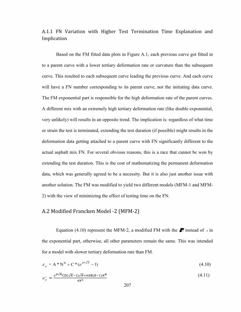
207
A.1.1 FN Variation with Higher Test Termination Time Explanation and
Implication
Based on the FM fitted data plots in Figure A.1, each previous curve got fitted in
to a parent curve with a lower tertiary deformation rate or curvature than the subsequent
curve. This resulted to each subsequent curve leading the previous curve. And each curve
will have a FN number corresponding to its parent curve, not the initiating data curve.
The FM exponential part is responsible for the high deformation rate of the parent curves.
A different mix with an extremely high tertiary deformation rate (like double exponential,
very unlikely) will results in an opposite trend. The implication is: regardless of what time
or strain the test is terminated, extending the test duration (if possible) might results in the
deformation data getting attached to a parent curve with FN significantly different to the
actual asphalt mix FN. For several obvious reasons, this is a race that cannot be won by
extending the test duration. This is the cost of mathematizing the permanent deformation
data, which was generally agreed to be a necessity. But it is also just another issue with
another solution. The FM was modified to yield two different models (MFM-1 and MFM-
2) with the view of minimizing the effect of testing time on the FN.
A.2 Modified Francken Model -2 (MFM-2)
Equation (4.10) represent the MFM-2, a modified FM with the N instead of N in
the exponential part, otherwise, all other parameters remain the same. This was intended
for a model with slower tertiary deformation rate than FM.
)1(*N*A= *B
NDp eC (4.10)
,,p
(4.11)
208
p = Permanent Strain Sustained by the HMA test Sample
,,p = Rate of change of the strain rate (second differential of p with respect to N ).
N = load cycle repetition in seconds
D & C B, A, are regression constants
Figure A.3 presents similar analysis as that in Figure A.1, but this time around the
data was fitted using MFM-2. The objective of slowing down the tertiary deformation of
the parent curve has been obviously achieved when both Figure A.1 and Figure A.3 are
compared. And the second objective, which was to minimize the effect of testing duration
on FN was also actualized as can be observed. The highest FN recorded was 576 for a test
time of 1510 seconds as opposed to 590 in the case of FM model fits. The questions still
remain: is this enough? how general is this improvements? These questions shall be
addressed in the subsequent paragraphs.
Figure A.3:Permanent Strain Data Fitted in to MFM-2 at Increasing level of the Tertiary
Flow.
450
950
1450
1950
2450
2950
3450
3950
4450
4950
0 500 1000 1500 2000 2500 3000
Pe
rman
en
t St
rain
(µ
st)
Load Cycle (s)
Mod. Francken Model-2 Fit
N740_(518) N860_(546) N980_(558) N1110_(565) N1510_(576)
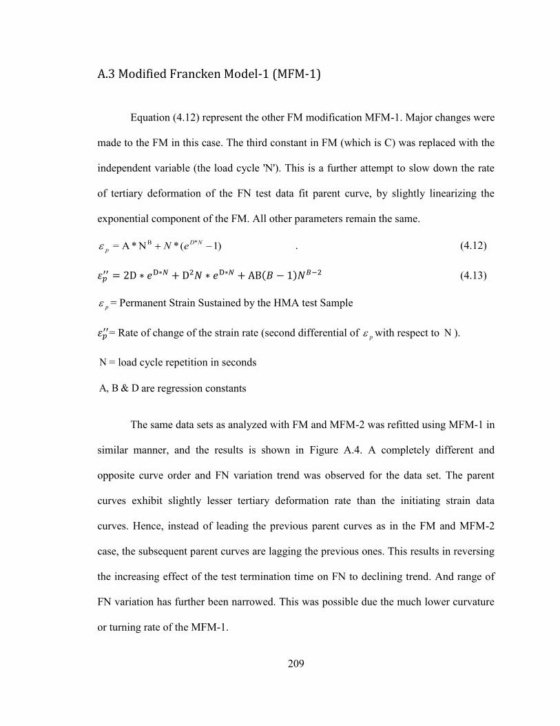
209
A.3 Modified Francken Model-1 (MFM-1)
Equation (4.12) represent the other FM modification MFM-1. Major changes were
made to the FM in this case. The third constant in FM (which is C) was replaced with the
independent variable (the load cycle 'N'). This is a further attempt to slow down the rate
of tertiary deformation of the FN test data fit parent curve, by slightly linearizing the
exponential component of the FM. All other parameters remain the same.
)1(*N*A= *B
NDp eN . (4.12)
(4.13)
p = Permanent Strain Sustained by the HMA test Sample
= Rate of change of the strain rate (second differential of p with respect to N ).
N = load cycle repetition in seconds
D & B A, are regression constants
The same data sets as analyzed with FM and MFM-2 was refitted using MFM-1 in
similar manner, and the results is shown in Figure A.4. A completely different and
opposite curve order and FN variation trend was observed for the data set. The parent
curves exhibit slightly lesser tertiary deformation rate than the initiating strain data
curves. Hence, instead of leading the previous parent curves as in the FM and MFM-2
case, the subsequent parent curves are lagging the previous ones. This results in reversing
the increasing effect of the test termination time on FN to declining trend. And range of
FN variation has further been narrowed. This was possible due the much lower curvature
or turning rate of the MFM-1.
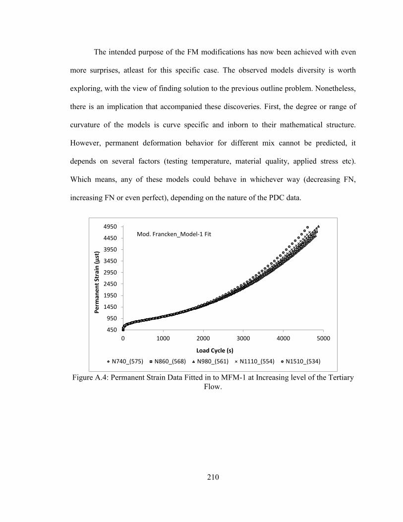
210
The intended purpose of the FM modifications has now been achieved with even
more surprises, atleast for this specific case. The observed models diversity is worth
exploring, with the view of finding solution to the previous outline problem. Nonetheless,
there is an implication that accompanied these discoveries. First, the degree or range of
curvature of the models is curve specific and inborn to their mathematical structure.
However, permanent deformation behavior for different mix cannot be predicted, it
depends on several factors (testing temperature, material quality, applied stress etc).
Which means, any of these models could behave in whichever way (decreasing FN,
increasing FN or even perfect), depending on the nature of the PDC data.
Figure A.4: Permanent Strain Data Fitted in to MFM-1 at Increasing level of the Tertiary
Flow.
450
950
1450
1950
2450
2950
3450
3950
4450
4950
0 1000 2000 3000 4000 5000
Pe
rman
en
t St
rain
(µ
st)
Load Cycle (s)
Mod. Francken_Model-1 Fit
N740_(575) N860_(568) N980_(561) N1110_(554) N1510_(534)
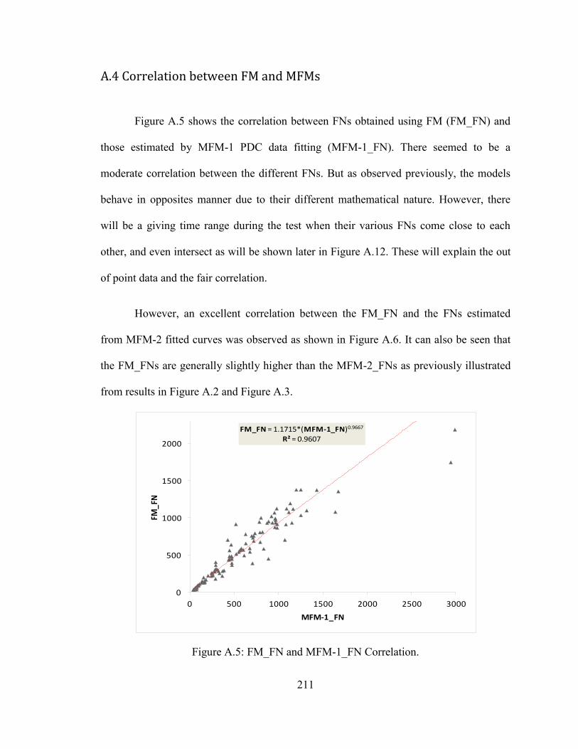
211
A.4 Correlation between FM and MFMs
Figure A.5 shows the correlation between FNs obtained using FM (FM_FN) and
those estimated by MFM-1 PDC data fitting (MFM-1_FN). There seemed to be a
moderate correlation between the different FNs. But as observed previously, the models
behave in opposites manner due to their different mathematical nature. However, there
will be a giving time range during the test when their various FNs come close to each
other, and even intersect as will be shown later in Figure A.12. These will explain the out
of point data and the fair correlation.
However, an excellent correlation between the FM_FN and the FNs estimated
from MFM-2 fitted curves was observed as shown in Figure A.6. It can also be seen that
the FM_FNs are generally slightly higher than the MFM-2_FNs as previously illustrated
from results in Figure A.2 and Figure A.3.
Figure A.5: FM_FN and MFM-1_FN Correlation.
FM_FN = 1.1715*(MFM-1_FN)0.9667
R² = 0.9607
0
500
1000
1500
2000
0 500 1000 1500 2000 2500 3000
FM_F
N
MFM-1_FN
212
Figure A.6: FM_FN and MFM-2_FN Correlation.
A.5 STANDARD FN LIMITS AND HMA FN VARIATION WITH TEST
TERMINATION TIME
To further demonstrate the implication of the test termination time effect on the
estimated FN values. A plots of the FN variation for numerous analyzed PDC data with
test duration was shown in Figure A.7 and Figure A.8. For the sake of plot clarity and
objectivity, only one set is plotted in cases where the data sets completely overlapped.
Figure A.7 show the FM and MFM-2 FN test time variation combined, as they
follow the same trend. The general trend is obvious, higher FN values for prolong tertiary
deformation. Another issue of great implication is the crossing of the FN limits for a
given recommended traffic category by a single HMA mix. This causes a lot of doubt as
to the validity of the FN specification limits and standard. It is obvious that the standard
and its related methods has more to tackle.
FM_FN = 1.0106*(MFM-2_FN)R² = 0.9964
0
500
1000
1500
2000
2500
0 500 1000 1500 2000 2500
FM_
FN
MFM-2_FN
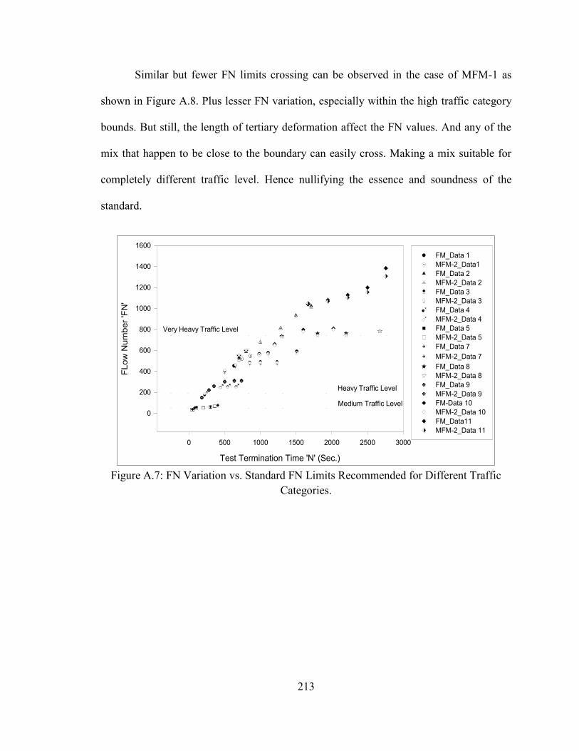
213
Similar but fewer FN limits crossing can be observed in the case of MFM-1 as
shown in Figure A.8. Plus lesser FN variation, especially within the high traffic category
bounds. But still, the length of tertiary deformation affect the FN values. And any of the
mix that happen to be close to the boundary can easily cross. Making a mix suitable for
completely different traffic level. Hence nullifying the essence and soundness of the
standard.
Figure A.7: FN Variation vs. Standard FN Limits Recommended for Different Traffic
Categories.
Test Termination Time 'N' (Sec.)
0 500 1000 1500 2000 2500 3000
FLow
Num
ber '
FN'
0
200
400
600
800
1000
1200
1400
1600
Very Heavy Traffic Level
Medium Traffic Level
Heavy Traffic Level
FM_Data 1 MFM-2_Data1 FM_Data 2 MFM-2_Data 2 FM_Data 3 MFM-2_Data 3 FM_Data 4 MFM-2_Data 4 FM_Data 5 MFM-2_Data 5 FM_Data 7 MFM-2_Data 7 FM_Data 8 MFM-2_Data 8FM_Data 9 MFM-2_Data 9 FM-Data 10 MFM-2_Data 10 FM_Data11 MFM-2_Data 11
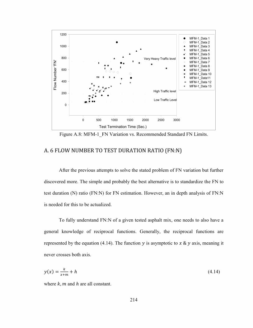
214
Figure A.8: MFM-1_FN Variation vs. Recommended Standard FN Limits.
A. 6 FLOW NUMBER TO TEST DURATION RATIO (FN:N)
After the previous attempts to solve the stated problem of FN variation but further
discovered more. The simple and probably the best alternative is to standardize the FN to
test duration (N) ratio (FN:N) for FN estimation. However, an in depth analysis of FN:N
is needed for this to be actualized.
To fully understand FN:N of a given tested asphalt mix, one needs to also have a
general knowledge of reciprocal functions. Generally, the reciprocal functions are
represented by the equation (4.14). The function is asymptotic to axis, meaning it
never crosses both axis.
(4.14)
where and are all constant.
Test Termination Time (Sec.)
0 500 1000 1500 2000 2500 3000
Flow
Num
ber '
FN'
0
200
400
600
800
1000
1200
Very Heavy Traffic level
High Traffic level
Low Traffic Level
MFM-1_Data 1 MFM-1_Data 2 MFM-1_Data 3 MFM-1_Data 4 MFM-1_Data 5 MFM-1_Data 6 MFM-1_Data 7 MFM-1_Data 8 MFM-1_Data 9 MFM-1_Data 10 MFM-1_Data11 MFM-1_Data 12 MFM-1_Data 13
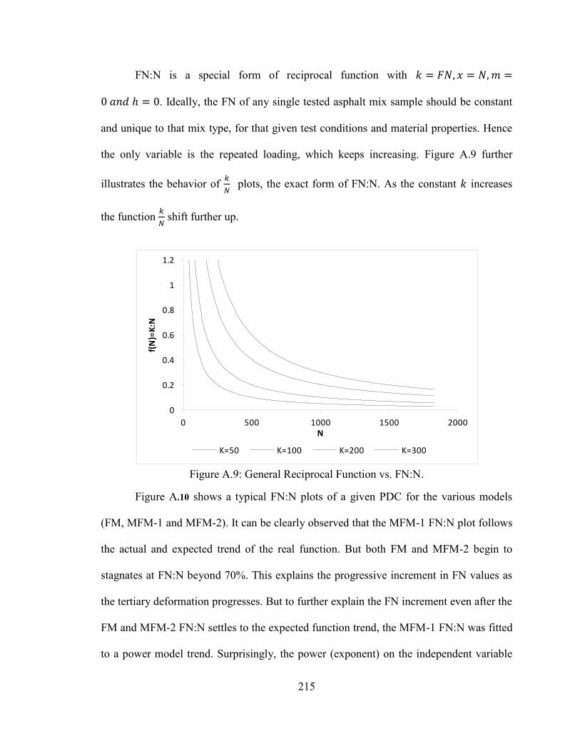
215
FN:N is a special form of reciprocal function with
. Ideally, the FN of any single tested asphalt mix sample should be constant
and unique to that mix type, for that given test conditions and material properties. Hence
the only variable is the repeated loading, which keeps increasing. Figure A.9 further
illustrates the behavior of
plots, the exact form of FN:N. As the constant increases
the function
shift further up.
Figure A.9: General Reciprocal Function vs. FN:N.
Figure A.10 shows a typical FN:N plots of a given PDC for the various models
(FM, MFM-1 and MFM-2). It can be clearly observed that the MFM-1 FN:N plot follows
the actual and expected trend of the real function. But both FM and MFM-2 begin to
stagnates at FN:N beyond 70%. This explains the progressive increment in FN values as
the tertiary deformation progresses. But to further explain the FN increment even after the
FM and MFM-2 FN:N settles to the expected function trend, the MFM-1 FN:N was fitted
to a power model trend. Surprisingly, the power (exponent) on the independent variable
0
0.2
0.4
0.6
0.8
1
1.2
0 500 1000 1500 2000
f(N
)=K
:N
N
K=50 K=100 K=200 K=300
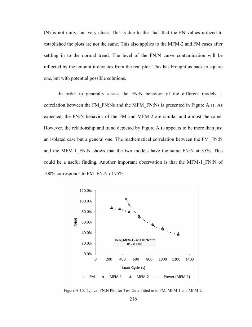
216
(N) is not unity, but very close. This is due to the fact that the FN values utilized to
established the plots are not the same. This also applies to the MFM-2 and FM cases after
settling in to the normal trend. The level of the FN:N curve contamination will be
reflected by the amount it deviates from the real plot. This has brought us back to square
one, but with potential possible solutions.
In order to generally assess the FN:N behavior of the different models, a
correlation between the FM_FN:Ns and the MFM_FN:Ns is presented in Figure A.11. As
expected, the FN:N behavior of the FM and MFM-2 are similar and almost the same.
However, the relationship and trend depicted by Figure A.10 appears to be more than just
an isolated case but a general one. The mathematical correlation between the FM_FN:N
and the MFM-1_FN:N shows that the two models have the same FN:N at 35%. This
could be a useful finding. Another important observation is that the MFM-1_FN:N of
100% corresponds to FM_FN:N of 75%.
Figure A.10: Typical FN:N Plot for Test Data Fitted in to FM, MFM-1 and MFM-2.
FN:N_MFM-1 = 631.88*N-1.047 R² = 0.9985
0.0%
20.0%
40.0%
60.0%
80.0%
100.0%
120.0%
0 200 400 600 800 1000 1200 1400
FN:N
Load Cycle (s)
FM MFM-1 MFM-2 Power (MFM-1)
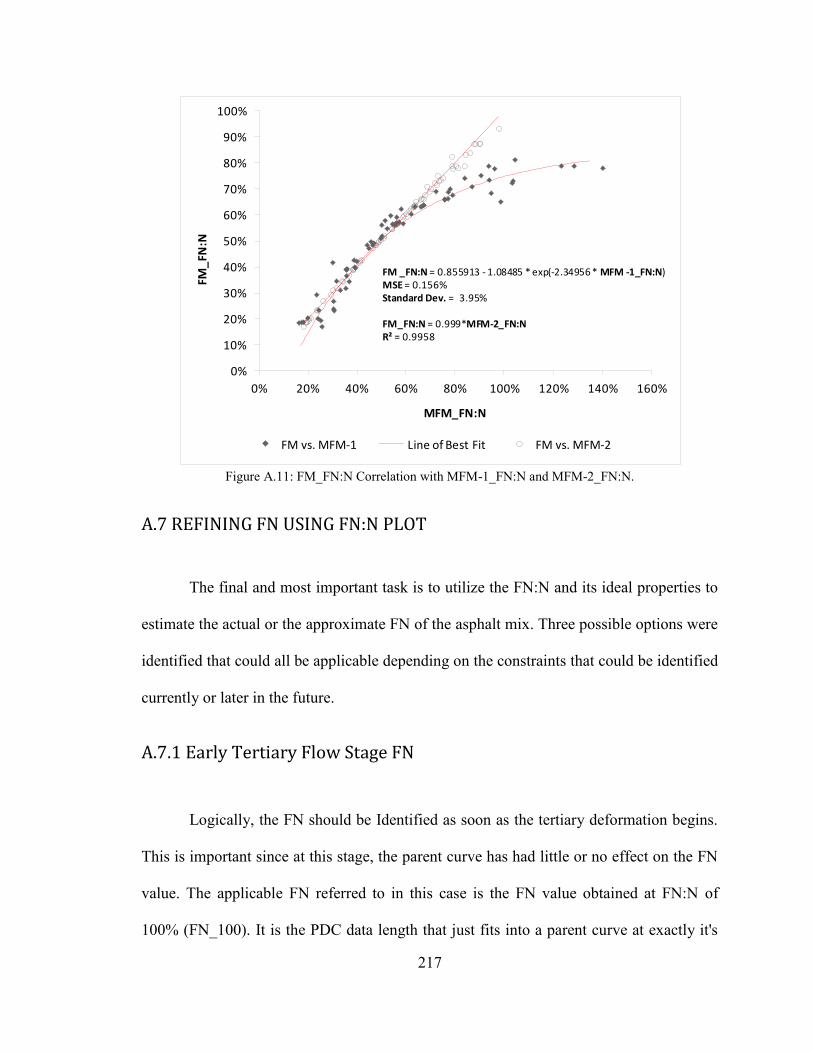
217
Figure A.11: FM_FN:N Correlation with MFM-1_FN:N and MFM-2_FN:N.
A.7 REFINING FN USING FN:N PLOT
The final and most important task is to utilize the FN:N and its ideal properties to
estimate the actual or the approximate FN of the asphalt mix. Three possible options were
identified that could all be applicable depending on the constraints that could be identified
currently or later in the future.
A.7.1 Early Tertiary Flow Stage FN
Logically, the FN should be Identified as soon as the tertiary deformation begins.
This is important since at this stage, the parent curve has had little or no effect on the FN
value. The applicable FN referred to in this case is the FN value obtained at FN:N of
100% (FN_100). It is the PDC data length that just fits into a parent curve at exactly it's
0%
10%
20%
30%
40%
50%
60%
70%
80%
90%
100%
0% 20% 40% 60% 80% 100% 120% 140% 160%
FM_
FN:N
MFM_FN:N
FM vs. MFM-1 Line of Best Fit FM vs. MFM-2
FM _FN:N = 0.855913 - 1.08485 * exp(-2.34956 * MFM -1_FN:N)MSE = 0.156%Standard Dev. = 3.95%
FM_FN:N = 0.999*MFM-2_FN:NR² = 0.9958
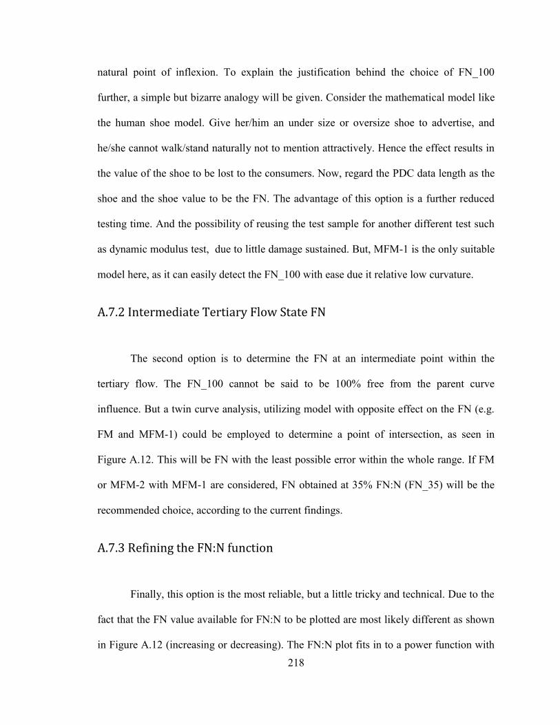
218
natural point of inflexion. To explain the justification behind the choice of FN_100
further, a simple but bizarre analogy will be given. Consider the mathematical model like
the human shoe model. Give her/him an under size or oversize shoe to advertise, and
he/she cannot walk/stand naturally not to mention attractively. Hence the effect results in
the value of the shoe to be lost to the consumers. Now, regard the PDC data length as the
shoe and the shoe value to be the FN. The advantage of this option is a further reduced
testing time. And the possibility of reusing the test sample for another different test such
as dynamic modulus test, due to little damage sustained. But, MFM-1 is the only suitable
model here, as it can easily detect the FN_100 with ease due it relative low curvature.
A.7.2 Intermediate Tertiary Flow State FN
The second option is to determine the FN at an intermediate point within the
tertiary flow. The FN_100 cannot be said to be 100% free from the parent curve
influence. But a twin curve analysis, utilizing model with opposite effect on the FN (e.g.
FM and MFM-1) could be employed to determine a point of intersection, as seen in
Figure A.12. This will be FN with the least possible error within the whole range. If FM
or MFM-2 with MFM-1 are considered, FN obtained at 35% FN:N (FN_35) will be the
recommended choice, according to the current findings.
A.7.3 Refining the FN:N function
Finally, this option is the most reliable, but a little tricky and technical. Due to the
fact that the FN value available for FN:N to be plotted are most likely different as shown
in Figure A.12 (increasing or decreasing). The FN:N plot fits in to a power function with
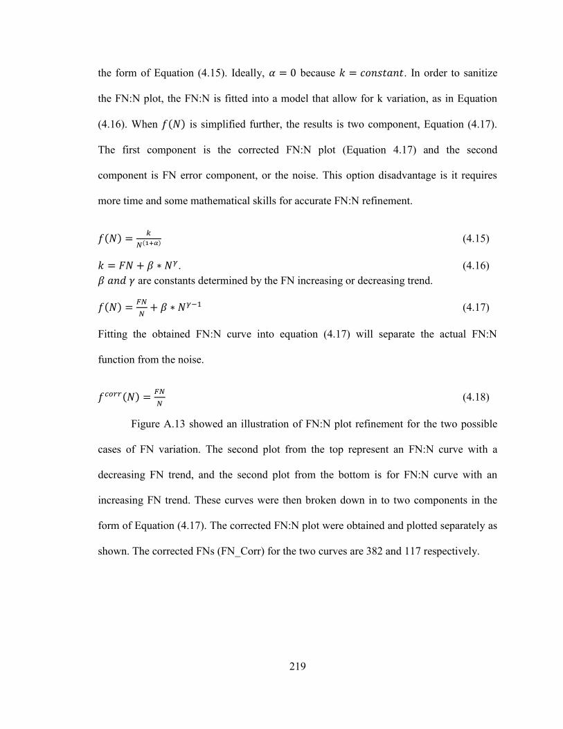
219
the form of Equation (4.15). Ideally, because . In order to sanitize
the FN:N plot, the FN:N is fitted into a model that allow for k variation, as in Equation
(4.16). When is simplified further, the results is two component, Equation (4.17).
The first component is the corrected FN:N plot (Equation 4.17) and the second
component is FN error component, or the noise. This option disadvantage is it requires
more time and some mathematical skills for accurate FN:N refinement.
(4.15)
. (4.16) are constants determined by the FN increasing or decreasing trend.
(4.17)
Fitting the obtained FN:N curve into equation (4.17) will separate the actual FN:N
function from the noise.
(4.18)
Figure A.13 showed an illustration of FN:N plot refinement for the two possible
cases of FN variation. The second plot from the top represent an FN:N curve with a
decreasing FN trend, and the second plot from the bottom is for FN:N curve with an
increasing FN trend. These curves were then broken down in to two components in the
form of Equation (4.17). The corrected FN:N plot were obtained and plotted separately as
shown. The corrected FNs (FN_Corr) for the two curves are 382 and 117 respectively.
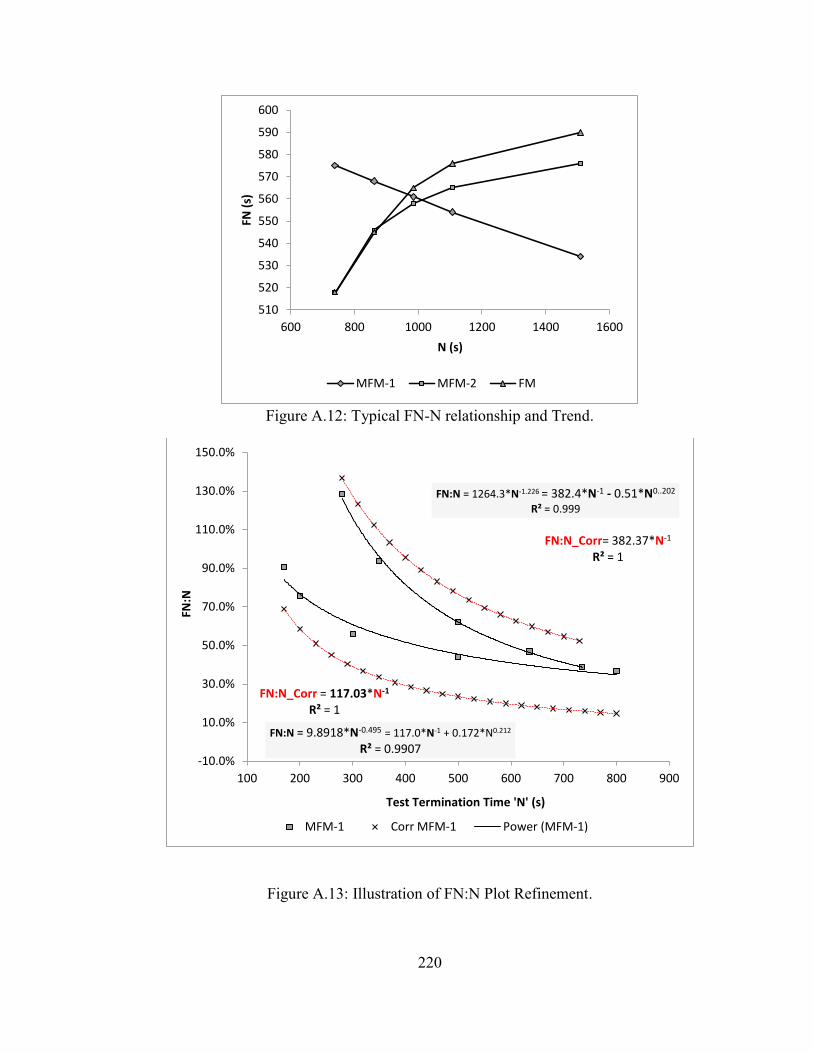
220
Figure A.12: Typical FN-N relationship and Trend.
Figure A.13: Illustration of FN:N Plot Refinement.
510
520
530
540
550
560
570
580
590
600
600 800 1000 1200 1400 1600
FN (
s)
N (s)
MFM-1 MFM-2 FM
FN:N = 1264.3*N-1.226 = 382.4*N-1 - 0.51*N0..202
R² = 0.999
FN:N_Corr= 382.37*N-1 R² = 1
FN:N = 9.8918*N-0.495 = 117.0*N-1 + 0.172*N0.212
R² = 0.9907
FN:N_Corr = 117.03*N-1 R² = 1
-10.0%
10.0%
30.0%
50.0%
70.0%
90.0%
110.0%
130.0%
150.0%
100 200 300 400 500 600 700 800 900
FN:N
Test Termination Time 'N' (s)
MFM-1 Corr MFM-1 Power (MFM-1)
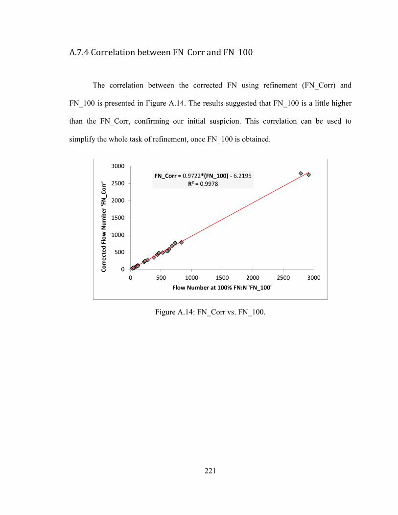
221
A.7.4 Correlation between FN_Corr and FN_100
The correlation between the corrected FN using refinement (FN_Corr) and
FN_100 is presented in Figure A.14. The results suggested that FN_100 is a little higher
than the FN_Corr, confirming our initial suspicion. This correlation can be used to
simplify the whole task of refinement, once FN_100 is obtained.
Figure A.14: FN_Corr vs. FN_100.
FN_Corr = 0.9722*(FN_100) - 6.2195 R² = 0.9978
0
500
1000
1500
2000
2500
3000
0 500 1000 1500 2000 2500 3000
Co
rre
cte
d F
low
Nu
mb
er
'FN
_Co
rr'
Flow Number at 100% FN:N 'FN_100'
222
A.8 How Tertiary Flow Length Affects the AC FN and Solution
Two new PDC models (MFM-1, MFM-2) were obtained by modifying the
Francken model (FM), and employed along with FM to investigate the effect of tertiary
flow length on HMA FN. Gauss-Newton algorithm was used to generated more than 360
FN data point from the three different PDC models (FM, MFM-1, MFM-2). The
mathematical structure of the PDC model used in analyzing the permanent strain data has
a huge influence on the resulting FN, and the FN variation trend as the tertiary
deformation stage progresses. Models with high curvature parent curves like FM and
MFM-2 mostly result in increasing FN values as the tertiary flow evolves. But low
curvature model like MFM-1 mainly results in lower FN as the HMA shear deformation
advanced. However, this models can behave whichever way, depending on the PDC data
rate of curvature change, which varies from mix type to test conditions. Mathematization
of the PDC data, which happens to be a necessity, was the result of the FN variation. The
estimated FN were found to represent the inflexion points of the fitted parent curve not
the initiation permanent strain data. The FN variation has resulted in a situation where a
single tested sample could be identified suitable for two different standard FN range
recommended traffic levels by AASHTO TP 79-15.
Flow number to test duration ratio (FN:N) has been identified as the simple and
ultimate solution for further standardization and refinement of FN test and FN value
respectively. Three possible options of utilizing FN:N for the aforementioned purpose
were recommended and highlighted. Methods of estimating the FN at early and
Intermediate tertiary flow stage and a complete refinement of the adulterated FN:N were

223
discussed and illustrated. Important correlations and between the refinement options were
also presented. The MFM-1 appears to be more robust than the FM and MFM-1 in the
utilization of FN:N curve.
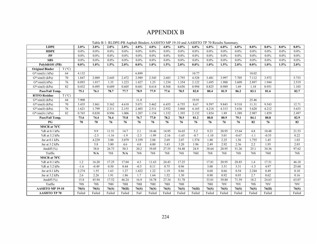
224
APPENDIX B Table B 1: RLDPE-PB Asphalt Binders AASHTO MP 19-10 and AASHTO TP 70 Results Summary.
LDPE 2.0% 2.0% 2.0% 2.0% 4.0% 4.0% 4.0% 4.0% 6.0% 6.0% 6.0% 6.0% 8.0% 8.0% 8.0% 8.0% HDPE 0.0% 0.0% 0.0% 0.0% 0.0% 0.0% 0.0% 0.0% 0.0% 0.0% 0.0% 0.0% 0.0% 0.0% 0.0% 0.0%
PP 0.0% 0.0% 0.0% 0.0% 0.0% 0.0% 0.0% 0.0% 0.0% 0.0% 0.0% 0.0% 0.0% 0.0% 0.0% 0.0% SBS 0.0% 0.0% 0.0% 0.0% 0.0% 0.0% 0.0% 0.0% 0.0% 0.0% 0.0% 0.0% 0.0% 0.0% 0.0% 0.0%
Polybilt101 (PB) 0.0% 1.0% 1.5% 2.0% 0.0% 1.0% 1.5% 2.0% 0.0% 1.0% 1.5% 2.0% 0.0% 1.0% 1.5% 2.0% Original Binder T (°C)
G*/sin(δ) ( kPa) 64 4.132 6.899 10.77 18.02 G*/sin(δ) (kPa) 70 1.847 2.089 2.645 2.472 2.989 2.545 2.683 2.793 4.528 3.481 3.997 7.705 7.112 3.972 5.753 G*/sin(δ) kPa) 76 0.893 1.017 1.35 1.223 1.427 1.25 1.234 1.354 2.122 1.695 1.988 3.609 2.897 1.944 2.519 G*/sin(δ) (kPa) 82 0.432 0.495 0.689 0.605 0.681 0.614 0.568 0.656 0.994 0.825 0.989 1.69 1.18 0.951 1.103
Pass/Fail Temp. 75.1 76.1 78.7 77.7 78.9 77.9 77.6 78.5 82.0 80.4 81.9 86.2 83.1 81.6 82.7 RTFO Residue T (°C)
G*/sin(δ) (kPa) 64 7.908 11.8 19.91 25.46 G*/sin(δ) (kPa) 70 3.435 3.861 5.362 4.618 5.071 5.462 6.455 6.755 8.67 9.597 9.843 9.518 11.31 9.543 12.71 G*/sin(δ) (kPa) 76 1.621 1.799 2.311 2.155 2.403 2.511 2.932 3.068 4.165 4.218 4.313 3.636 5.628 4.212 5.633 G*/sin(δ) ( kPa) 82 0.765 0.838 0.996 1.006 1.207 1.154 1.332 1.393 2.132 1.854 1.89 1.389 2.987 1.859 2.497
Pass/Fail Temp. 73.6 74.4 76.4 75.8 76.7 77.0 78.2 78.5 81.2 80.8 80.9 79.1 84.1 80.8 82.9 PG 70 70 76 76 76 76 76 76 76 76 76 76 82 76 82
MSCR at 76oC %R at 0.1 kPa 9.9 11.51 14.7 2.1 10.46 14.95 16.65 5.2 9.23 20.95 15.64 4.8 10.48 21.53 %R at 3.2 kPa -2.5 -1.16 -1.9 -2.3 -1.99 -2.16 -1.65 -0.7 -1.10 5.01 -0.67 -1.1 -0.55 0.22 Jnr at 0.1 kPa 4.229 3.00 3.079 3.359 2.88 2.69 2.07 1.574 1.80 2.25 1.56 1.755 1.45 1.03 Jnr at 3.2 kPa 5.8 3.80 4.6 4.0 4.00 3.43 3.20 1.96 2.49 2.92 2.36 2.2 1.95 2.03
Jnrdiff (%) 38.0 26.73 50.3 20.2 39.05 27.55 54.48 24.9 38.64 20.95 51.26 25.1 34.36 97.62 Traffic N/A 76S N/A 76S 76S 76S 76S 76H 76S 76S 76S 76S 76H 76S
MSCR at 70oC %R at 0.1 kPa 1.2 16.20 17.25 17.04 4.3 11.63 24.43 17.25
17.81 20.95 28.85 1.4 17.51 46.18
%R at 3.2 kPa -1.6 -0.49 0.50 0.44 -0.5 0.11 0.75 0.96 3.08 3.51 3.31 -1.5 4.97 25.60 Jnr at 0.1 kPa 2.274 1.55 1.63 1.27 1.422 1.22 1.19 0.86 0.68 0.66 0.54 2.244 0.49 0.10 Jnr at 3.2 kPa 2.6 2.26 1.91 1.86 1.7 1.64 1.52 1.30 0.90 0.92 0.93 2.7 0.62 0.16
Jnrdiff (%) 15.8 45.94 17.52 46.24 16.9 34.78 27.34 51.78 33.01 39.80 71.59 18.2 24.63 63.07 Traffic 70S 70S 70H 70H 70H 70H 70H 70H 70H 70V 70V 70S 70V 70V
AASHTO MP 19-10 70(S) 70(S) 76(S) 70(H) 76(S) 76(S) 76(S) 76(S) 76(H) 76(S) 76(S) 76(S) 76(S) 76(H) 76(S) AASHTO TP 70 Failed Failed Failed Failed Fail Failed Failed Failed Failed Failed Failed Failed Failed Failed Failed
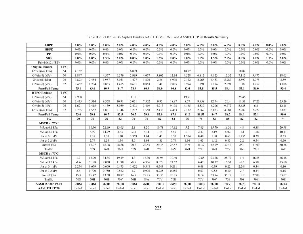
225
Table B 2: RLDPE-SBS Asphalt Binders AASHTO MP 19-10 and AASHTO TP 70 Results Summary.
LDPE 2.0% 2.0% 2.0% 2.0% 4.0% 4.0% 4.0% 4.0% 6.0% 6.0% 6.0% 6.0% 8.0% 8.0% 8.0% 8.0% HDPE 0.0% 0.0% 0.0% 0.0% 0.0% 0.0% 0.0% 0.0% 0.0% 0.0% 0.0% 0.0% 0.0% 0.0% 0.0% 0.0%
PP 0.0% 0.0% 0.0% 0.0% 0.0% 0.0% 0.0% 0.0% 0.0% 0.0% 0.0% 0.0% 0.0% 0.0% 0.0% 0.0% SBS 0.0% 1.0% 1.5% 2.0% 0.0% 1.0% 1.5% 2.0% 0.0% 1.0% 1.5% 2.0% 0.0% 1.0% 1.5% 2.0%
Polybilt101 (PB) 0.0% 0.0% 0.0% 0.0% 0.0% 0.0% 0.0% 0.0% 0.0% 0.0% 0.0% 0.0% 0.0% 0.0% 0.0% 0.0% Original Binder T (°C) G*/sin(δ) ( kPa) 64 4.132 6.899 10.77 18.02 G*/sin(δ) (kPa) 70 1.847 4.577 6.579 2.989 4.077 5.802 12.14 4.528 6.812 9.123 13.32 7.112 9.477 18.05 G*/sin(δ) kPa) 76 0.893 2.454 1.987 3.051 1.427 1.876 2.86 5.908 2.122 2.965 4.453 5.987 2.897 4.075 8.59 G*/sin(δ) (kPa) 82 0.432 1.204 0.863 1.415 0.681 0.863 1.41 2.875 0.994 1.291 2.174 2.691 1.18 1.752 4.088
Pass/Fail Temp. 75.1 83.6 80.9 84.7 78.9 80.9 84.9 90.8 82.0 83.8 88.5 89.4 83.1 86.0 93.4 RTFO Residue T (°C) G*/sin(δ) (kPa) 64 7.908 11.8 19.91 25.46 G*/sin(δ) (kPa) 70 3.435 7.514 9.358 10.91 5.071 7.502 9.92 18.87 8.67 9.958 12.74 20.4 11.31 17.26 25.29 G*/sin(δ) (kPa) 76 1.621 3.415 4.139 5.059 2.403 3.419 4.913 9.198 4.165 4.539 6.206 9.772 5.628 6.2 12.15 G*/sin(δ) ( kPa) 82 0.765 1.552 1.831 2.346 1.207 1.558 2.433 4.483 2.132 2.069 3.023 4.681 2.987 2.227 5.837
Pass/Fail Temp. 73.6 79.4 80.7 82.5 76.7 79.4 82.9 87.9 81.2 81.53 84.7 88.2 84.1 82.1 90.0 PG 70 76 76 82 76 76 82 82 76 76 82 88 82 82 **
MSCR at 76oC %R at 0.1 kPa 10.90 22.69 13.05 2.1 8.30 10.78 19.12 5.2 7.85 15.70 16.36 4.8 6.88 29.98 %R at 3.2 kPa 3.90 14.29 3.63 -2.3 3.34 1.14 8.57 -0.7 2.47 2.19 5.02 -1.1 1.78 10.13 Jnr at 0.1 kPa 2.38 1.30 1.20 3.359 1.64 1.43 0.57 1.574 0.48 1.00 0.63 1.755 0.39 0.33 Jnr at 3.2 kPa 2.79 1.54 1.54 4.0 1.98 1.85 0.74 1.96 1.63 1.42 0.83 2.2 0.54 0.50
Jnrdiff (%) 17.07 18.08 28.88 20.2 20.55 29.38 28.57 24.9 31.39 42.79 32.42 25.1 37.00 50.56 Traffic 76S 76H 76H 76S 76H 76H 76V 76H 76H 76H 76V 76S 76H 76E
MSCR at 70oC %R at 0.1 kPa 1.2 13.90 34.35 19.39 4.3 16.30 21.96 30.40 17.85 23.28 28.77 1.4 16.88 46.18 %R at 3.2 kPa -1.6 7.198 9.030 11.90 -0.5 4.336 8.028 21.57 6.47 10.37 15.51 -1.5 6.78 25.60 Jnr at 0.1 kPa 2.274 0.679 0.660 0.473 1.422 0.548 0.543 0.211 0.48 0.39 0.22 2.244 0.34 0.10 Jnr at 3.2 kPa 2.6 0.790 0.750 0.562 1.7 0.976 0.725 0.255 0.63 0.52 0.30 2.7 0.44 0.16
Jnrdiff (%) 15.8 16.42 13.68 18.87 16.9 78.25 33.35 20.85 32.39 33.94 35.17 18.2 27.00 63.07 Traffic 70S 70H 70H 70V 70H N/A 70V 70E 70V 70V 70E 70S 70E 70E
AASHTO MP 19-10 70(S) 76(S) 76(H) 76(H) 76(S) 76(H) 76(H) 76(V) 76(H) 76(H) 76(H) 76(V) 76(S) 76(H) 76(E) AASHTO TP 70 Failed Failed Failed Failed Failed Failed Failed Failed Failed Failed Failed Failed Failed Failed Failed
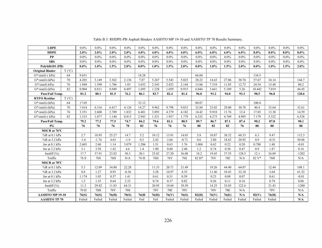
226
Table B 3: RHDPE-PB Asphalt Binders AASHTO MP 19-10 and AASHTO TP 70 Results Summary.
LDPE 0.0% 0.0% 0.0% 0.0% 0.0% 0.0% 0.0% 0.0% 0.0% 0.0% 0.0% 0.0% 0.0% 0.0% 0.0% 0.0% HDPE 2.0% 2.0% 2.0% 2.0% 4.0% 4.0% 4.0% 4.0% 6.0% 6.0% 6.0% 6.0% 8.0% 8.0% 8.0% 8.0%
PP 0.0% 0.0% 0.0% 0.0% 0.0% 0.0% 0.0% 0.0% 0.0% 0.0% 0.0% 0.0% 0.0% 0.0% 0.0% 0.0% SBS 0.0% 0.0% 0.0% 0.0% 0.0% 0.0% 0.0% 0.0% 0.0% 0.0% 0.0% 0.0% 0.0% 0.0% 0.0% 0.0%
Polybilt101 (PB) 0.0% 1.0% 1.5% 2.0% 0.0% 1.0% 1.5% 2.0% 0.0% 1.0% 1.5% 2.0% 0.0% 1.0% 1.5% 2.0% Original Binder T (°C) G*/sin(δ) ( kPa) 64 9.651 18.28 66.04 134.5 G*/sin(δ) (kPa) 70 4.203 3.149 3.362 2.136 7.87 5.267 5.543 5.023 28.22 14.63 27.06 30.76 57.67 34.14 144.7 G*/sin(δ) kPa) 76 1.949 1.598 1.786 1.03 3.652 2.543 2.423 2.144 13.06 7.318 11.85 12.72 24.54 15.48 80.2 G*/sin(δ) (kPa) 82 0.904 0.811 0.949 0.497 1.695 1.228 1.059 0.915 6.044 3.661 5.189 5.26 10.442 7.019 44.45
Pass/Fail Temp. 81.2 80.1 81.5 76.2 86.1 83.7 82.4 81.4 96.0 93.2 94.0 93.3 98.5 96.8 120.6 RTFO Residue T (°C) G*/sin(δ) (kPa) 64 17.05 33.12 80.07 100.4 G*/sin(δ) (kPa) 70 7.414 6.316 6.417 4.126 14.27 9.962 9.798 9.833 32.84 23.02 29.00 30.78 40.4 33.64 32.61 G*/sin(δ) (kPa) 76 3.351 2.608 2.709 1.832 6.481 3.893 4.379 4.182 14.42 9.918 11.76 12.4 17.03 13.38 14.59 G*/sin(δ) ( kPa) 82 1.515 1.077 1.144 0.813 2.943 1.521 1.957 1.779 6.332 4.273 4.769 4.995 7.179 5.322 6.528
Pass/Fail Temp. 79.2 77.2 77.5 74.7 84.2 79.6 81.1 80.5 89.7 86.7 87.1 87.4 90.2 87.8 90.1 PG 76 76 76 70 82 76 76 76 88 82 82 76 88 88 88
MSCR at 76oC %R at 0.1 kPa 2.7 10.95 25.27 14.7 5.2 10.12 13.91 14.03 5.8 10.87 38.32 60.33 6.3 9.47 112.3 %R at 3.2 kPa -1.6 -1.74 4.63 -1.9 0.3 2.42 2.66 -0.71 0.6 2.80 18.62 20.92 0.9 -0.51 50.88 Jnr at 0.1 kPa 2.603 2.60 1.14 3.079 1.206 1.51 0.63 1.76 1.004 0.62 0.22 0.20 0.788 1.48 -0.01 Jnr at 3.2 kPa 3.1 3.58 1.42 4.6 1.4 1.90 0.80 2.40 1.2 0.74 0.30 0.47 0.9 1.87 0.16
Jnrdiff (%) 17.7 37.91 23.82 50.3 20.1 25.82 27.20 36.08 18.2 19.45 37.55 128.5 12.1 26.09 -1202 Traffic 76 S 76S 76H N/A 76 H 76H 76V 76S 82 H* 76V 76E N/A 82 V* 76H N/A
MSCR at 70oC %R at 0.1 kPa 5.3 12.09 34.80 22.28 11.33 20.71 21.49 19.26 44.40 64.07 12.44 108.1 %R at 3.2 kPa 0.8 1.27 0.93 -0.36 3.28 10.97 4.35 11.46 10.43 32.10 3.64 61.52 Jnr at 0.1 kPa 1.174 1.05 0.57 1.41 0.61 0.31 0.59 0.23 0.08 0.07 0.61 -0.01 Jnr at 3.2 kPa 1.3 1.35 0.64 2.32 0.74 0.37 0.82 0.26 0.11 0.16 0.74 0.06
Jnrdiff (%) 11.3 29.42 11.83 64.31 20.95 19.60 39.59 14.25 33.05 122.6 21.43 -1200 Traffic 70 H 70H 70V 70S 70V 70E 70V 70V 70E N/A 70V N/A
AASHTO MP 19-10 76(S) 76(S) 76(H) 70(S) 76(H 76(H) 76(V) 76(S) 82(H) 76(V) 76(E) N/A 82(V) 76(H) N/A AASHTO TP 70 Failed Failed Failed Failed Fail Fail Failed Failed Failed Failed Failed Failed Failed Failed N/A
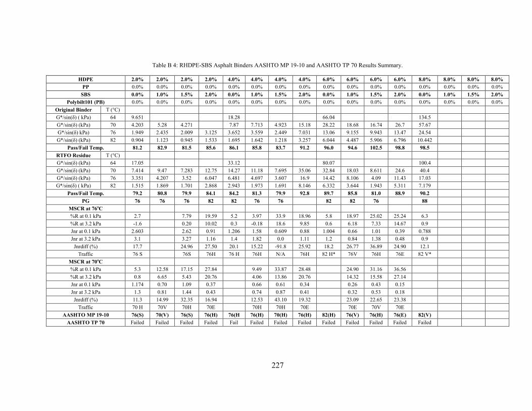
227
Table B 4: RHDPE-SBS Asphalt Binders AASHTO MP 19-10 and AASHTO TP 70 Results Summary.
HDPE 2.0% 2.0% 2.0% 2.0% 4.0% 4.0% 4.0% 4.0% 6.0% 6.0% 6.0% 6.0% 8.0% 8.0% 8.0% 8.0% PP 0.0% 0.0% 0.0% 0.0% 0.0% 0.0% 0.0% 0.0% 0.0% 0.0% 0.0% 0.0% 0.0% 0.0% 0.0% 0.0%
SBS 0.0% 1.0% 1.5% 2.0% 0.0% 1.0% 1.5% 2.0% 0.0% 1.0% 1.5% 2.0% 0.0% 1.0% 1.5% 2.0% Polybilt101 (PB) 0.0% 0.0% 0.0% 0.0% 0.0% 0.0% 0.0% 0.0% 0.0% 0.0% 0.0% 0.0% 0.0% 0.0% 0.0% 0.0%
Original Binder T (°C) G*/sin(δ) ( kPa) 64 9.651 18.28 66.04 134.5 G*/sin(δ) (kPa) 70 4.203 5.28 4.271 7.87 7.713 4.923 15.18 28.22 18.68 16.74 26.7 57.67 G*/sin(δ) kPa) 76 1.949 2.435 2.009 3.125 3.652 3.559 2.449 7.031 13.06 9.155 9.943 13.47 24.54 G*/sin(δ) (kPa) 82 0.904 1.123 0.945 1.533 1.695 1.642 1.218 3.257 6.044 4.487 5.906 6.796 10.442
Pass/Fail Temp. 81.2 82.9 81.5 85.6 86.1 85.8 83.7 91.2 96.0 94.6 102.5 98.8 98.5 RTFO Residue T (°C) G*/sin(δ) (kPa) 64 17.05 33.12 80.07 100.4 G*/sin(δ) (kPa) 70 7.414 9.47 7.283 12.75 14.27 11.18 7.695 35.06 32.84 18.03 8.611 24.6 40.4 G*/sin(δ) (kPa) 76 3.351 4.207 3.52 6.047 6.481 4.697 3.607 16.9 14.42 8.106 4.09 11.43 17.03 G*/sin(δ) ( kPa) 82 1.515 1.869 1.701 2.868 2.943 1.973 1.691 8.146 6.332 3.644 1.943 5.311 7.179
Pass/Fail Temp. 79.2 80.8 79.9 84.1 84.2 81.3 79.9 92.8 89.7 85.8 81.0 88.9 90.2 PG 76 76 76 82 82 76 76 82 82 76 88
MSCR at 76oC %R at 0.1 kPa 2.7 7.79 19.59 5.2 3.97 33.9 18.96 5.8 18.97 25.02 25.24 6.3 %R at 3.2 kPa -1.6 0.20 10.02 0.3 -0.18 18.6 9.85 0.6 6.18 7.33 14.67 0.9 Jnr at 0.1 kPa 2.603 2.62 0.91 1.206 1.58 0.609 0.88 1.004 0.66 1.01 0.39 0.788 Jnr at 3.2 kPa 3.1 3.27 1.16 1.4 1.82 0.0 1.11 1.2 0.84 1.38 0.48 0.9
Jnrdiff (%) 17.7 24.96 27.50 20.1 15.22 -91.8 25.92 18.2 26.77 36.89 24.90 12.1 Traffic 76 S 76S 76H 76 H 76H N/A 76H 82 H* 76V 76H 76E 82 V*
MSCR at 70oC %R at 0.1 kPa 5.3 12.58 17.15 27.84 9.49 33.87 28.48 24.90 31.16 36.56 %R at 3.2 kPa 0.8 6.65 5.43 20.76 4.06 13.86 20.76 14.32 15.58 27.14 Jnr at 0.1 kPa 1.174 0.70 1.09 0.37 0.66 0.61 0.34 0.26 0.43 0.15 Jnr at 3.2 kPa 1.3 0.81 1.44 0.43 0.74 0.87 0.41 0.32 0.53 0.18
Jnrdiff (%) 11.3 14.99 32.35 16.94 12.53 43.10 19.32 23.09 22.65 23.38 Traffic 70 H 70V 70H 70E 70H 70H 70E 70E 70V 70E
AASHTO MP 19-10 76(S) 70(V) 76(S) 76(H) 76(H 76(H) 70(H) 76(H) 82(H) 76(V) 76(H) 76(E) 82(V) AASHTO TP 70 Failed Failed Failed Failed Fail Failed Failed Failed Failed Failed Failed Failed Failed
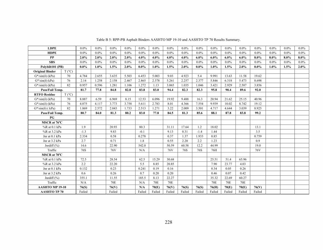
228
Table B 5: RPP-PB Asphalt Binders AASHTO MP 19-10 and AASHTO TP 70 Results Summary.
LDPE 0.0% 0.0% 0.0% 0.0% 0.0% 0.0% 0.0% 0.0% 0.0% 0.0% 0.0% 0.0% 0.0% 0.0% 0.0% 0.0% HDPE 0.0% 0.0% 0.0% 0.0% 0.0% 0.0% 0.0% 0.0% 0.0% 0.0% 0.0% 0.0% 0.0% 0.0% 0.0% 0.0%
PP 2.0% 2.0% 2.0% 2.0% 4.0% 4.0% 4.0% 4.0% 6.0% 6.0% 6.0% 6.0% 8.0% 8.0% 8.0% 8.0% SBS 0.0% 0.0% 0.0% 0.0% 0.0% 0.0% 0.0% 0.0% 0.0% 0.0% 0.0% 0.0% 0.0% 0.0% 0.0% 0.0%
Polybilt101 (PB) 0.0% 1.0% 1.5% 2.0% 0.0% 1.0% 1.5% 2.0% 0.0% 1.0% 1.5% 2.0% 0.0% 1.0% 1.5% 2.0% Original Binder T (°C) G*/sin(δ) (kPa) 70 4.784 2.655 3.635 5.503 6.453 5.003 9.03 4.923 5.4 9.991 13.63 11.58 19.62 G*/sin(δ) kPa) 76 2.14 1.258 2.158 2.467 2.865 2.378 5.261 2.257 2.377 5.846 6.318 5.473 8.698 G*/sin(δ) (kPa) 82 0.957 0.596 1.281 1.106 1.272 1.13 3.065 1.035 1.046 3.421 2.929 2.587 3.856
Pass/Fail Temp. 81.7 77.8 84.8 82.8 83.8 83.0 94.4 82.3 82.3 95.8 90.4 89.6 92.0 RTFO Residue T (°C) G*/sin(δ) (kPa) 70 8.887 6.59 6.969 8.15 12.53 6.096 19.92 9.488 16.3 20.94 21.62 25.15 40.96 G*/sin(δ) (kPa) 76 4.075 4.117 3.773 3.758 5.611 2.783 8.01 4.366 7.554 9.939 10.02 8.742 19.12 G*/sin(δ) ( kPa) 82 1.869 2.572 2.043 1.733 2.513 1.271 3.22 2.009 3.501 4.717 4.644 3.039 8.925
Pass/Fail Temp. 80.7 84.0 81.3 80.2 83.0 77.8 84.5 81.3 85.6 88.1 87.8 83.8 99.2 PG
MSCR at 76oC %R at 0.1 kPa 1.9 20.93 80.3 31.11 17.64 1.2 18.02 13.1 %R at 3.2 kPa -1.3 9.83 -0.1 9.13 0.31 -1.4 1.44 3.5 Jnr at 0.1 kPa 2.334 0.58 0.278 0.37 1.37 1.933 0.85 0.759 Jnr at 3.2 kPa 2.7 0.71 1.8 0.55 2.20 2.2 1.23 0.9
Jnrdiff (%) 14.6 22.90 542.0 50.59 60.58 12.2 44.99 19.0 Traffic 76S 76V N/A 76V 76S 76S 76H 76V
MSCR at 70oC %R at 0.1 kPa 72.5 28.54 62.5 15.29 30.68 25.51 51.4 65.96 %R at 3.2 kPa 2.2 22.20 5.5 8.85 20.85 7.90 23.77 4.03 Jnr at 0.1 kPa 0.132 0.23 0.241 0.19 0.16 0.34 0.05 0.26 Jnr at 3.2 kPa 0.6 0.26 0.7 0.20 0.20 0.46 0.07 0.42
Jnrdiff (%) 355.1 11.55 185.5 8.13 22.27 35.32 22.69 60.27 Traffic N/A 70E N/A 70E 70E 70E 70E 70E
AASHTO MP 19-10 76(S) 76(V) N/A 70(E) 76(V) 76(S) 76(S) 76(H) 70(E) 70(E) 76(V) AASHTO TP 70 Failed Failed Failed Failed Failed Failed Failed Failed Failed Failed Failed
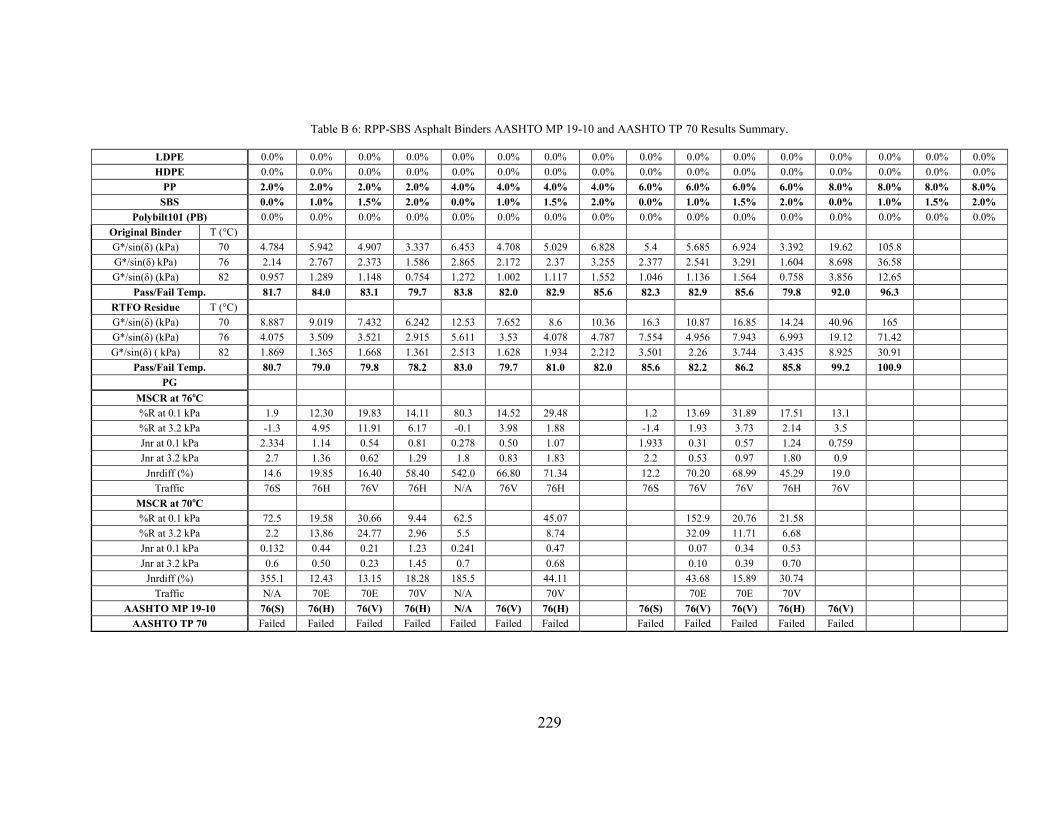
229
Table B 6: RPP-SBS Asphalt Binders AASHTO MP 19-10 and AASHTO TP 70 Results Summary.
LDPE 0.0% 0.0% 0.0% 0.0% 0.0% 0.0% 0.0% 0.0% 0.0% 0.0% 0.0% 0.0% 0.0% 0.0% 0.0% 0.0% HDPE 0.0% 0.0% 0.0% 0.0% 0.0% 0.0% 0.0% 0.0% 0.0% 0.0% 0.0% 0.0% 0.0% 0.0% 0.0% 0.0%
PP 2.0% 2.0% 2.0% 2.0% 4.0% 4.0% 4.0% 4.0% 6.0% 6.0% 6.0% 6.0% 8.0% 8.0% 8.0% 8.0% SBS 0.0% 1.0% 1.5% 2.0% 0.0% 1.0% 1.5% 2.0% 0.0% 1.0% 1.5% 2.0% 0.0% 1.0% 1.5% 2.0%
Polybilt101 (PB) 0.0% 0.0% 0.0% 0.0% 0.0% 0.0% 0.0% 0.0% 0.0% 0.0% 0.0% 0.0% 0.0% 0.0% 0.0% 0.0% Original Binder T (°C) G*/sin(δ) (kPa) 70 4.784 5.942 4.907 3.337 6.453 4.708 5.029 6.828 5.4 5.685 6.924 3.392 19.62 105.8 G*/sin(δ) kPa) 76 2.14 2.767 2.373 1.586 2.865 2.172 2.37 3.255 2.377 2.541 3.291 1.604 8.698 36.58 G*/sin(δ) (kPa) 82 0.957 1.289 1.148 0.754 1.272 1.002 1.117 1.552 1.046 1.136 1.564 0.758 3.856 12.65
Pass/Fail Temp. 81.7 84.0 83.1 79.7 83.8 82.0 82.9 85.6 82.3 82.9 85.6 79.8 92.0 96.3 RTFO Residue T (°C) G*/sin(δ) (kPa) 70 8.887 9.019 7.432 6.242 12.53 7.652 8.6 10.36 16.3 10.87 16.85 14.24 40.96 165 G*/sin(δ) (kPa) 76 4.075 3.509 3.521 2.915 5.611 3.53 4.078 4.787 7.554 4.956 7.943 6.993 19.12 71.42 G*/sin(δ) ( kPa) 82 1.869 1.365 1.668 1.361 2.513 1.628 1.934 2.212 3.501 2.26 3.744 3.435 8.925 30.91
Pass/Fail Temp. 80.7 79.0 79.8 78.2 83.0 79.7 81.0 82.0 85.6 82.2 86.2 85.8 99.2 100.9 PG
MSCR at 76oC %R at 0.1 kPa 1.9 12.30 19.83 14.11 80.3 14.52 29.48 1.2 13.69 31.89 17.51 13.1 %R at 3.2 kPa -1.3 4.95 11.91 6.17 -0.1 3.98 1.88 -1.4 1.93 3.73 2.14 3.5 Jnr at 0.1 kPa 2.334 1.14 0.54 0.81 0.278 0.50 1.07 1.933 0.31 0.57 1.24 0.759 Jnr at 3.2 kPa 2.7 1.36 0.62 1.29 1.8 0.83 1.83 2.2 0.53 0.97 1.80 0.9
Jnrdiff (%) 14.6 19.85 16.40 58.40 542.0 66.80 71.34 12.2 70.20 68.99 45.29 19.0 Traffic 76S 76H 76V 76H N/A 76V 76H 76S 76V 76V 76H 76V
MSCR at 70oC %R at 0.1 kPa 72.5 19.58 30.66 9.44 62.5 45.07 152.9 20.76 21.58 %R at 3.2 kPa 2.2 13.86 24.77 2.96 5.5 8.74 32.09 11.71 6.68 Jnr at 0.1 kPa 0.132 0.44 0.21 1.23 0.241 0.47 0.07 0.34 0.53 Jnr at 3.2 kPa 0.6 0.50 0.23 1.45 0.7 0.68 0.10 0.39 0.70
Jnrdiff (%) 355.1 12.43 13.15 18.28 185.5 44.11 43.68 15.89 30.74 Traffic N/A 70E 70E 70V N/A
70V 70E 70E 70V
AASHTO MP 19-10 76(S) 76(H) 76(V) 76(H) N/A 76(V) 76(H) 76(S) 76(V) 76(V) 76(H) 76(V) AASHTO TP 70 Failed Failed Failed Failed Failed Failed Failed Failed Failed Failed Failed Failed
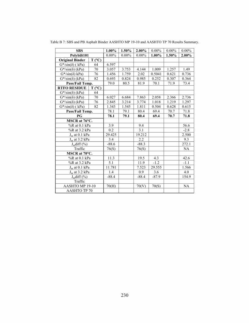
230
Table B 7: SBS and PB Asphalt Binder AASHTO MP 19-10 and AASHTO TP 70 Results Summary.
SBS 1.00% 1.50% 2.00% 0.00% 0.00% 0.00% Polybilt101 0.00% 0.00% 0.00% 1.00% 1.50% 2.00%
Original Binder T (°C) G*/sin(δ) ( kPa) 64 6.597 G*/sin(δ) (kPa) 70 3.057 3.753 4.144 1.009 1.257 1.49 G*/sin(δ) kPa) 76 1.456 1.759 2.02 0.5041 0.621 0.736 G*/sin(δ) (kPa) 82 0.693 0.824 0.985 0.252 0.307 0.364
Pass/Fail Temp. 79.0 80.5 81.9 70.1 71.9 73.4 RTFO RESIDUE T (°C) G*/sin(δ) (kPa) 64 G*/sin(δ) (kPa) 70 6.027 6.684 7.863 2.058 2.366 2.736
G*/sin(δ) (kPa) 76 2.845 3.214 3.774 1.018 1.219 1.297 G*/sin(δ) ( kPa) 82 1.343 1.545 1.811 0.504 0.628 0.615
Pass/Fail Temp. 78.1 79.1 80.4 69.4 70.7 71.8 PG 78.1 79.1 80.4 69.4 70.7 71.8
MSCR at 76°C. %R at 0.1 kPa 3.9 9.4 56.6 %R at 3.2 kPa 0.2 3.1 -2.8 Jnr at 0.1 kPa 29.425 19.212 2.500 Jnr at 3.2 kPa 3.4 2.2 9.3
Jnrdiff (%) -88.6 -88.3 272.1 Traffic 76(S) 76(S) NA
MSCR at 70°C. %R at 0.1 kPa 11.3 19.5 4.3 42.6 %R at 3.2 kPa 5.1 11.9 -1.2 -1.1 Jnr at 0.1 kPa 11.781 7.523 29.555 1.566 Jnr at 3.2 kPa 1.4 0.9 3.6 4.0
Jnrdiff (%) -88.4 -88.4 -87.9 154.9 Traffic AASHTO MP 19-10 70(H) 70(V) 70(S) NA
AASHTO TP 70
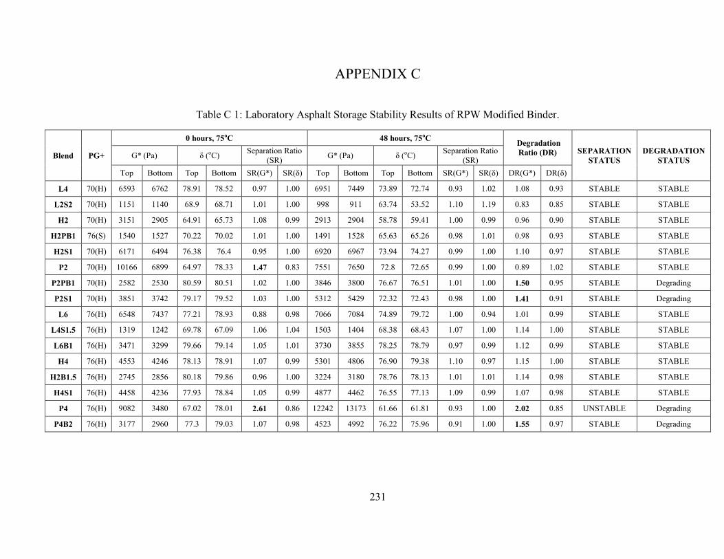
231
APPENDIX C
Table C 1: Laboratory Asphalt Storage Stability Results of RPW Modified Binder.
Blend PG+
0 hours, 75oC 48 hours, 75oC Degradation Ratio (DR) SEPARATION
STATUS DEGRADATION
STATUS G* (Pa) δ (oC) Separation Ratio (SR) G* (Pa) δ (oC) Separation Ratio
(SR) Top Bottom Top Bottom SR(G*) SR(δ) Top Bottom Top Bottom SR(G*) SR(δ) DR(G*) DR(δ)
L4 70(H) 6593 6762 78.91 78.52 0.97 1.00 6951 7449 73.89 72.74 0.93 1.02 1.08 0.93 STABLE STABLE
L2S2 70(H) 1151 1140 68.9 68.71 1.01 1.00 998 911 63.74 53.52 1.10 1.19 0.83 0.85 STABLE STABLE
H2 70(H) 3151 2905 64.91 65.73 1.08 0.99 2913 2904 58.78 59.41 1.00 0.99 0.96 0.90 STABLE STABLE
H2PB1 76(S) 1540 1527 70.22 70.02 1.01 1.00 1491 1528 65.63 65.26 0.98 1.01 0.98 0.93 STABLE STABLE
H2S1 70(H) 6171 6494 76.38 76.4 0.95 1.00 6920 6967 73.94 74.27 0.99 1.00 1.10 0.97 STABLE STABLE
P2 70(H) 10166 6899 64.97 78.33 1.47 0.83 7551 7650 72.8 72.65 0.99 1.00 0.89 1.02 STABLE STABLE
P2PB1 70(H) 2582 2530 80.59 80.51 1.02 1.00 3846 3800 76.67 76.51 1.01 1.00 1.50 0.95 STABLE Degrading
P2S1 70(H) 3851 3742 79.17 79.52 1.03 1.00 5312 5429 72.32 72.43 0.98 1.00 1.41 0.91 STABLE Degrading
L6 76(H) 6548 7437 77.21 78.93 0.88 0.98 7066 7084 74.89 79.72 1.00 0.94 1.01 0.99 STABLE STABLE
L4S1.5 76(H) 1319 1242 69.78 67.09 1.06 1.04 1503 1404 68.38 68.43 1.07 1.00 1.14 1.00 STABLE STABLE
L6B1 76(H) 3471 3299 79.66 79.14 1.05 1.01 3730 3855 78.25 78.79 0.97 0.99 1.12 0.99 STABLE STABLE
H4 76(H) 4553 4246 78.13 78.91 1.07 0.99 5301 4806 76.90 79.38 1.10 0.97 1.15 1.00 STABLE STABLE
H2B1.5 76(H) 2745 2856 80.18 79.86 0.96 1.00 3224 3180 78.76 78.13 1.01 1.01 1.14 0.98 STABLE STABLE
H4S1 76(H) 4458 4236 77.93 78.84 1.05 0.99 4877 4462 76.55 77.13 1.09 0.99 1.07 0.98 STABLE STABLE
P4 76(H) 9082 3480 67.02 78.01 2.61 0.86 12242 13173 61.66 61.81 0.93 1.00 2.02 0.85 UNSTABLE Degrading
P4B2 76(H) 3177 2960 77.3 79.03 1.07 0.98 4523 4992 76.22 75.96 0.91 1.00 1.55 0.97 STABLE Degrading
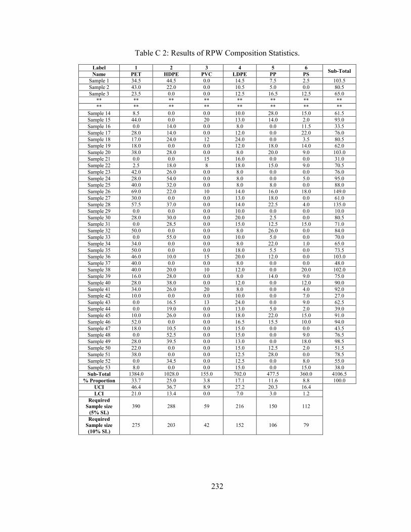
232
Table C 2: Results of RPW Composition Statistics.
Label 1 2 3 4 5 6 Sub-Total Name PET HDPE PVC LDPE PP PS Sample 1 34.5 44.5 0.0 14.5 7.5 2.5 103.5 Sample 2 43.0 22.0 0.0 10.5 5.0 0.0 80.5 Sample 3 23.5 0.0 0.0 12.5 16.5 12.5 65.0
** ** ** ** ** ** ** ** ** ** ** ** ** ** ** **
Sample 14 8.5 0.0 0.0 10.0 28.0 15.0 61.5 Sample 15 44.0 0.0 20 13.0 14.0 2.0 93.0 Sample 16 0.0 14.0 0.0 8.0 0.0 11.5 33.5 Sample 17 28.0 14.0 0.0 12.0 0.0 22.0 76.0 Sample 18 17.0 24.0 12 24.0 0.0 3.5 80.5 Sample 19 18.0 0.0 0.0 12.0 18.0 14.0 62.0 Sample 20 38.0 28.0 0.0 8.0 20.0 9.0 103.0 Sample 21 0.0 0.0 15 16.0 0.0 0.0 31.0 Sample 22 2.5 18.0 8 18.0 15.0 9.0 70.5 Sample 23 42.0 26.0 0.0 8.0 0.0 0.0 76.0 Sample 24 28.0 54.0 0.0 8.0 0.0 5.0 95.0 Sample 25 40.0 32.0 0.0 8.0 8.0 0.0 88.0 Sample 26 69.0 22.0 10 14.0 16.0 18.0 149.0 Sample 27 30.0 0.0 0.0 13.0 18.0 0.0 61.0 Sample 28 57.5 37.0 0.0 14.0 22.5 4.0 135.0 Sample 29 0.0 0.0 0.0 10.0 0.0 0.0 10.0 Sample 30 28.0 30.0 0.0 20.0 2.5 0.0 80.5 Sample 31 0.0 28.5 0.0 15.0 12.5 15.0 71.0 Sample 32 50.0 0.0 0.0 8.0 26.0 0.0 84.0 Sample 33 0.0 55.0 0.0 10.0 5.0 0.0 70.0 Sample 34 34.0 0.0 0.0 8.0 22.0 1.0 65.0 Sample 35 50.0 0.0 0.0 18.0 5.5 0.0 73.5 Sample 36 46.0 10.0 15 20.0 12.0 0.0 103.0 Sample 37 40.0 0.0 0.0 8.0 0.0 0.0 48.0 Sample 38 40.0 20.0 10 12.0 0.0 20.0 102.0 Sample 39 16.0 28.0 0.0 8.0 14.0 9.0 75.0 Sample 40 28.0 38.0 0.0 12.0 0.0 12.0 90.0 Sample 41 34.0 26.0 20 8.0 0.0 4.0 92.0 Sample 42 10.0 0.0 0.0 10.0 0.0 7.0 27.0 Sample 43 0.0 16.5 13 24.0 0.0 9.0 62.5 Sample 44 0.0 19.0 0.0 13.0 5.0 2.0 39.0 Sample 45 10.0 26.0 0.0 18.0 22.0 15.0 91.0 Sample 46 52.0 0.0 0.0 16.5 15.5 10.0 94.0 Sample 47 18.0 10.5 0.0 15.0 0.0 0.0 43.5 Sample 48 0.0 52.5 0.0 15.0 0.0 9.0 76.5 Sample 49 28.0 39.5 0.0 13.0 0.0 18.0 98.5 Sample 50 22.0 0.0 0.0 15.0 12.5 2.0 51.5 Sample 51 38.0 0.0 0.0 12.5 28.0 0.0 78.5 Sample 52 0.0 34.5 0.0 12.5 0.0 8.0 55.0 Sample 53 8.0 0.0 0.0 15.0 0.0 15.0 38.0 Sub-Total 1384.0 1028.0 155.0 702.0 477.5 360.0 4106.5
% Proportion 33.7 25.0 3.8 17.1 11.6 8.8 100.0 UCI 46.4 36.7 8.9 27.2 20.3 16.4 LCI 21.0 13.4 0.0 7.0 3.0 1.2 Required
Sample size (5% SL)
390 288 59 216 150 112
Required Sample size (10% SL)
275 203 42 152 106 79
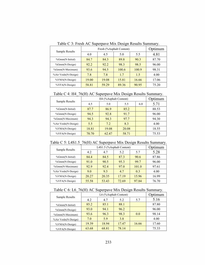
233
Table C 3: Fresh AC Superpave Mix Design Results Summary.
Sample Results Fresh (%Asphalt Content) Optimum
4.0 4.5 5.0 5.5 4.81 %Gmm(N-Initial) 84.7 84.3 89.8 90.3 87.70 %Gmm(N-Design) 92.2 92.2 98.3 98.5 96.00
%Gmm(N-Maximum) 93.6 94.5 100.6 100.9 98.31 %Air Voids(N-Design) 7.8 7.8 1.7 1.5 4.00
%VMA(N-Design) 19.00 19.08 15.81 16.66 17.06 %VFA(N-Design) 58.81 59.29 89.36 90.95 75.20
Table C 4: H4_76(H) AC Superpave Mix Design Results Summary.
Sample Results H4 (%Asphalt Content) Optimum
4.5 5.0 5.5 6.0 5.71 %Gmm(N-Initial) 87.7 86.9 85.2 88.53 %Gmm(N-Design) 94.5 92.8 91.7 96.00
%Gmm(N-Maximum) 94.3 94.3 97.7 94.30 %Air Voids(N-Design) 5.5 7.2 8.3 4.00
%VMA(N-Design) 18.81 19.08 20.08 18.55 %VFA(N-Design) 70.70 62.47 58.71 75.53
Table C 5: L4S1.5_76(H) AC Superpave Mix Design Results Summary.
Sample Results L4S1.5 (%Asphalt Content) Optimum
4.2 4.7 5.2 5.7 5.28 %Gmm(N-Initial) 84.4 84.5 87.3 90.6 87.86 %Gmm(N-Design) 91.0 90.5 95.3 99.7 96.00
%Gmm(N-Maximum) 92.9 92.4 97.0 101.0 97.61 %Air Voids(N-Design) 9.0 9.5 4.7 0.3 4.00
%VMA(N-Design) 20.27 20.35 17.19 15.96 16.99 %VFA(N-Design) 55.58 53.43 72.69 97.84 76.70
Table C 6: L6_76(H) AC Superpave Mix Design Results Summary.
Sample Results L6 (%Asphalt Content) Optimum
4.2 4.7 5.2 5.7 5.16 %Gmm(N-Initial) 85.2 85.1 88.1 87.80 %Gmm(N-Design) 93.0 94.1 96.2 96.00
%Gmm(N-Maximum) 93.6 96.3 98.3 0.0 98.14 %Air Voids(N-Design) 7.0 5.9 3.8 4.00
%VMA(N-Design) 19.39 18.94 17.47 16.66 17.60 %VFA(N-Design) 63.68 68.81 78.14 75.33
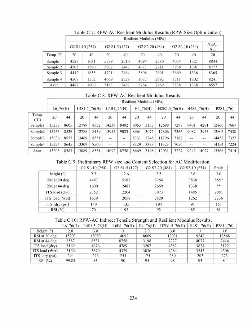
234
Table C 7: RPW-AC Resilient Modulus Results (RPW Size Optimization).
Resilient Modulus (MPa)
G2 S1-10 (254) G2 S1-5 (127) G2 S2-20 (484) G2 S2-10 (254) NEAT AC.
Temp. oC 20 40 20 40 20 40 20 40 20 Sample 1 4527 1631 5539 2510 4094 2580 4034 1321 8844 Sample 2 4503 1580 5802 2447 4077 2711 3936 1391 8777 Sample 3 4412 1635 4721 2464 3808 2691 3669 1336 8365 Sample 4 4507 1552 4669 2528 3077 2692 3711 1302 8241
Aver. 4487 1600 5183 2487 3764 2669 3838 1338 8557
Table C 8: RPW-AC Resilient Modulus Results.
Resilient Modulus (MPa)
L6_76(H) L4S1.5_76(H) L6B1_76(H) H4_76(H) H2B1.5_76(H) H4S1_76(H) P2S1_(76) Temp. (oC) 20 44 20 44 20 44 20 44 20 44 20 44 20 44
Sample1 15288 8605 12789 8552 14239 8492 9053 3133 12698 7298 9401 4201 12860 7667 Sample2 15263 8526 12788 8459 13945 9023 8961 3077 12806 7366 9082 3953 12806 7438 Sample3 15036 8573 13469 8551 -- -- 8331 3248 11296 7188 -- -- 14452 7327 Sample4 15224 8645 13309 8560 -- -- 8329 3333 11323 7056 -- -- 14154 7224
Aver. 15203 8587 13089 8531 14092 8758 8669 3198 12031 7227 9242 4077 13568 7414
Table C 9: Preliminary RPW size and Content Selection for AC Modification. G2 S1-10 (254) G2 S1-5 (127) G2 S2-20 (484) G2 S2-10 (254) Fresh
height (") 2.7 2.6 2.5 2.6 3.0 RM at 20 deg 4487 5183 3764 3838 8557 RM at 44 deg 1600 2487 2669 1338 ** ITS load (dry) 2352 2204 3073 1485 2881 ITS load (Wet) 1639 2058 2820 1262 2336 ITS -dry (psi) 140 135 194 91 151
RSI (%) 70 93 92 85 81
Table C 10: RPW-AC Indirect Tensile Strength and Resilient Modulus Results. L6_76(H) L4S1.5_76(H) L6B1_76(H) H4_76(H) H2B1.5_76(H) H4S1_76(H) P2S1_(76)
height (") 2.8 3.0 3 2.9 3.0 3 3.0 RM at 20 deg 15203 13089 14092 8669 12031 9242 13568 RM at 44 deg 8587 8531 8758 3198 7227 4077 7414 ITS load (dry) 5169 4676 4789 3207 4382 3824 5122 ITS load (Wet) 5160 3870 4329 3036 4284 3543 4308 ITS -dry (psi) 294 246 254 175 230 203 273
RSI (%) 99.83 83 90 95 98 93 84
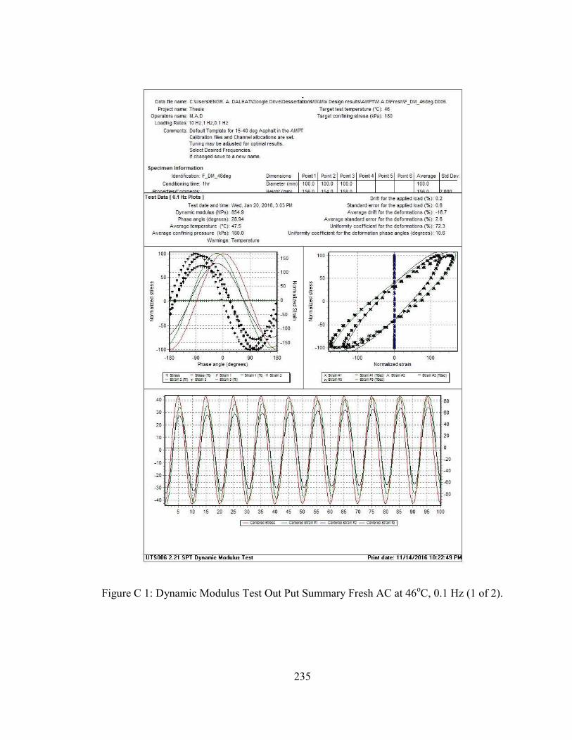
235
Figure C 1: Dynamic Modulus Test Out Put Summary Fresh AC at 46oC, 0.1 Hz (1 of 2).
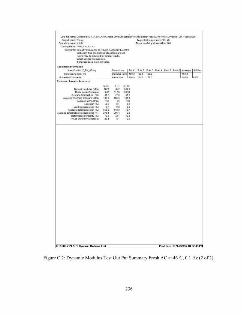
236
Figure C 2: Dynamic Modulus Test Out Put Summary Fresh AC at 46oC, 0.1 Hz (2 of 2).
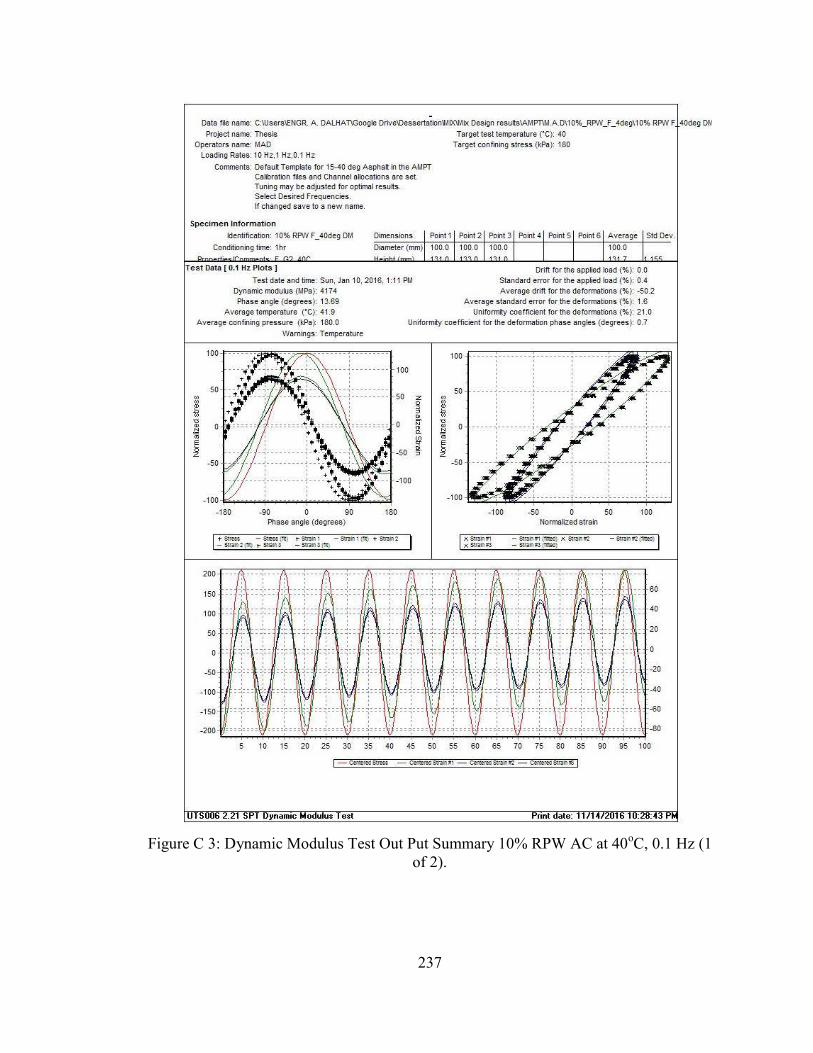
237
Figure C 3: Dynamic Modulus Test Out Put Summary 10% RPW AC at 40oC, 0.1 Hz (1
of 2).
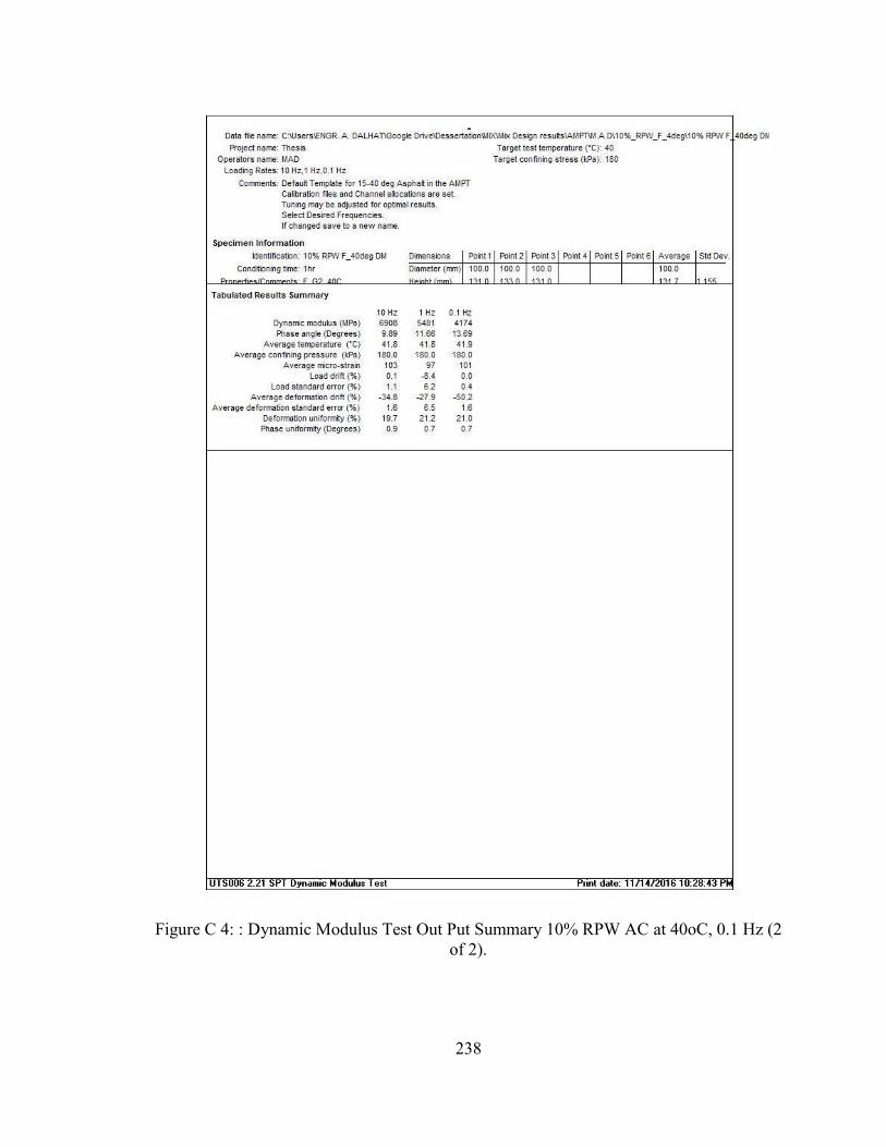
238
Figure C 4: : Dynamic Modulus Test Out Put Summary 10% RPW AC at 40oC, 0.1 Hz (2 of 2).
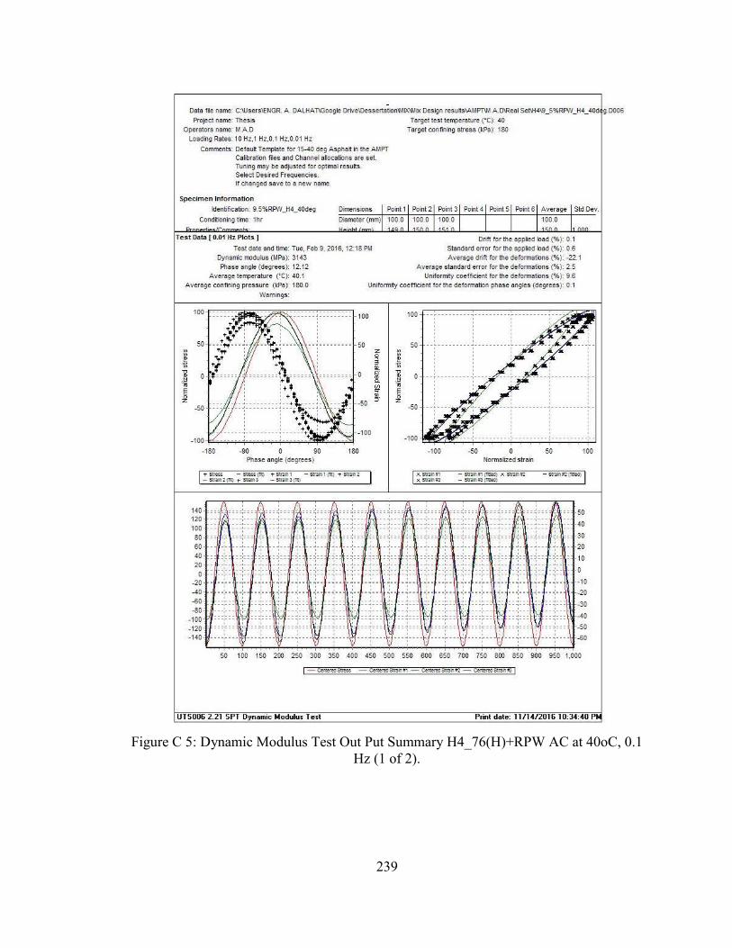
239
Figure C 5: Dynamic Modulus Test Out Put Summary H4_76(H)+RPW AC at 40oC, 0.1
Hz (1 of 2).
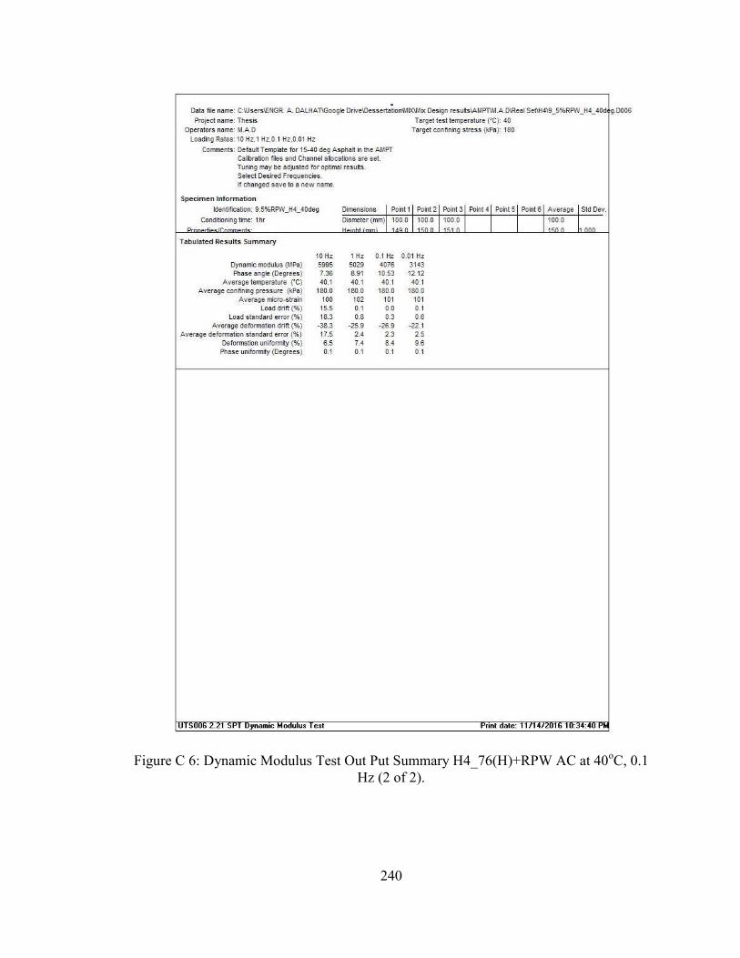
240
Figure C 6: Dynamic Modulus Test Out Put Summary H4_76(H)+RPW AC at 40oC, 0.1 Hz (2 of 2).
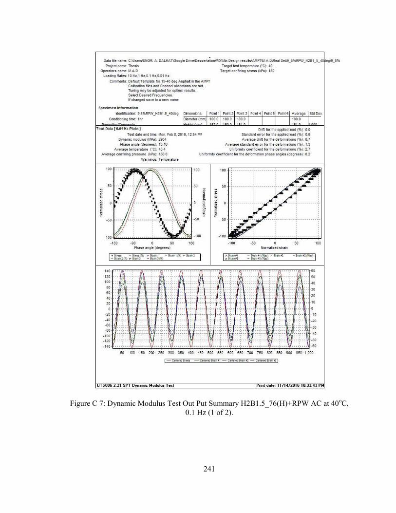
241
Figure C 7: Dynamic Modulus Test Out Put Summary H2B1.5_76(H)+RPW AC at 40oC, 0.1 Hz (1 of 2).
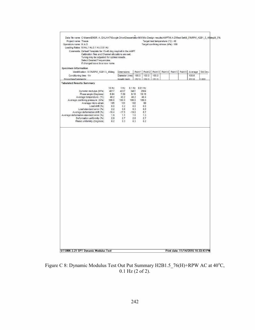
242
Figure C 8: Dynamic Modulus Test Out Put Summary H2B1.5_76(H)+RPW AC at 40oC, 0.1 Hz (2 of 2).
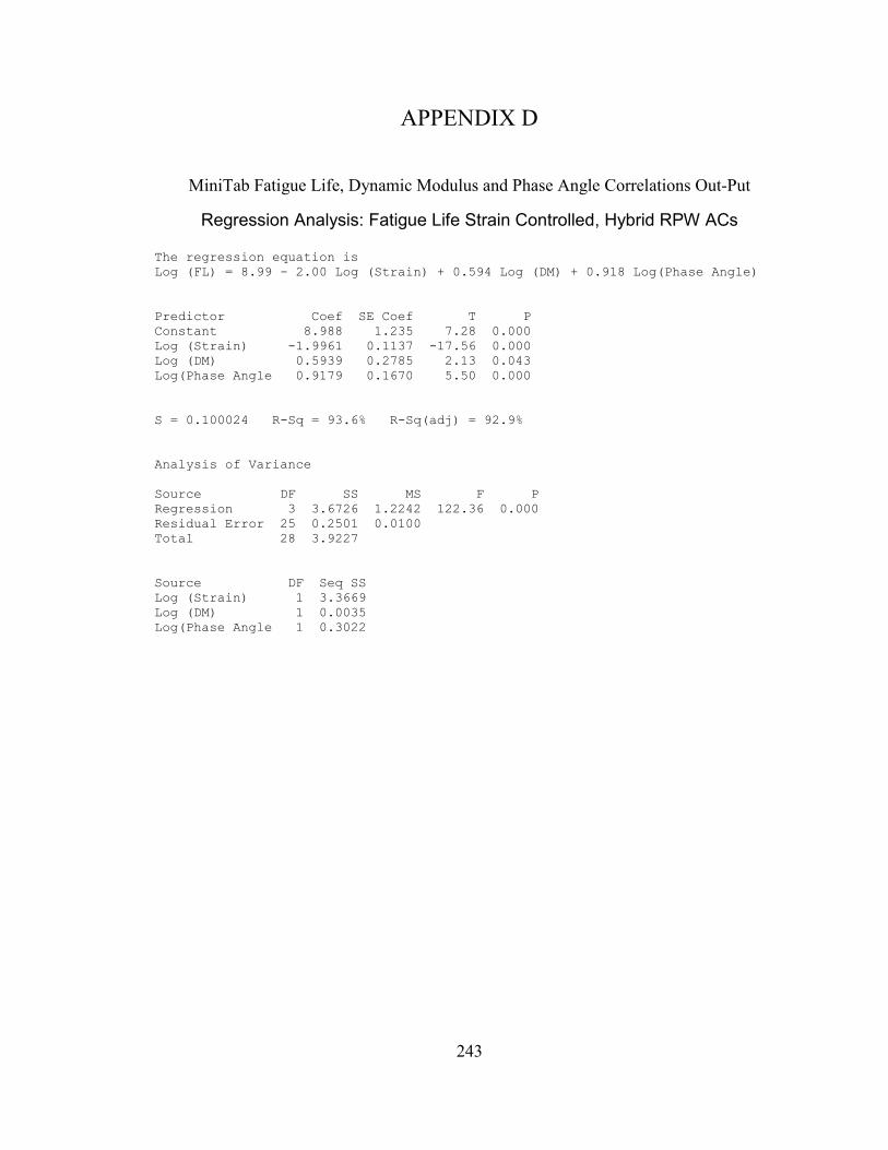
243
APPENDIX D
MiniTab Fatigue Life, Dynamic Modulus and Phase Angle Correlations Out-Put
Regression Analysis: Fatigue Life Strain Controlled, Hybrid RPW ACs The regression equation is
Log (FL) = 8.99 - 2.00 Log (Strain) + 0.594 Log (DM) + 0.918 Log(Phase Angle)
Predictor Coef SE Coef T P
Constant 8.988 1.235 7.28 0.000
Log (Strain) -1.9961 0.1137 -17.56 0.000
Log (DM) 0.5939 0.2785 2.13 0.043
Log(Phase Angle 0.9179 0.1670 5.50 0.000
S = 0.100024 R-Sq = 93.6% R-Sq(adj) = 92.9%
Analysis of Variance
Source DF SS MS F P
Regression 3 3.6726 1.2242 122.36 0.000
Residual Error 25 0.2501 0.0100
Total 28 3.9227
Source DF Seq SS
Log (Strain) 1 3.3669
Log (DM) 1 0.0035
Log(Phase Angle 1 0.3022
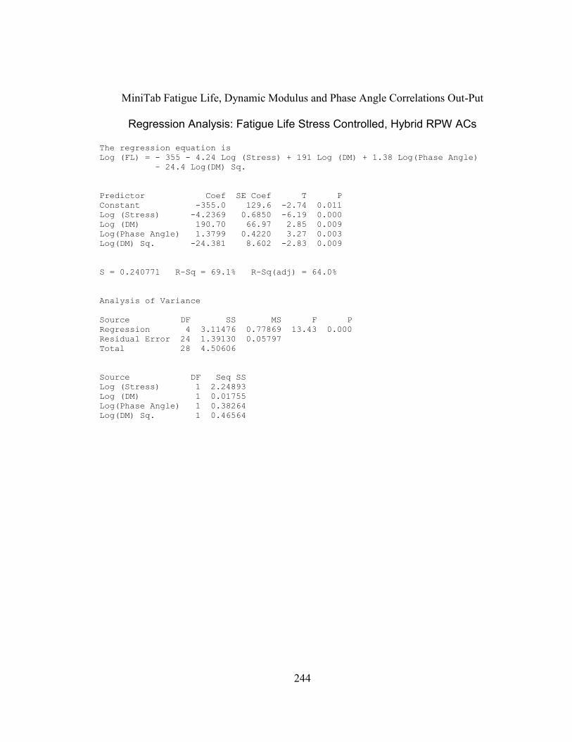
244
MiniTab Fatigue Life, Dynamic Modulus and Phase Angle Correlations Out-Put
Regression Analysis: Fatigue Life Stress Controlled, Hybrid RPW ACs The regression equation is
Log (FL) = - 355 - 4.24 Log (Stress) + 191 Log (DM) + 1.38 Log(Phase Angle)
- 24.4 Log(DM) Sq.
Predictor Coef SE Coef T P
Constant -355.0 129.6 -2.74 0.011
Log (Stress) -4.2369 0.6850 -6.19 0.000
Log (DM) 190.70 66.97 2.85 0.009
Log(Phase Angle) 1.3799 0.4220 3.27 0.003
Log(DM) Sq. -24.381 8.602 -2.83 0.009
S = 0.240771 R-Sq = 69.1% R-Sq(adj) = 64.0%
Analysis of Variance
Source DF SS MS F P
Regression 4 3.11476 0.77869 13.43 0.000
Residual Error 24 1.39130 0.05797
Total 28 4.50606
Source DF Seq SS
Log (Stress) 1 2.24893
Log (DM) 1 0.01755
Log(Phase Angle) 1 0.38264
Log(DM) Sq. 1 0.46564
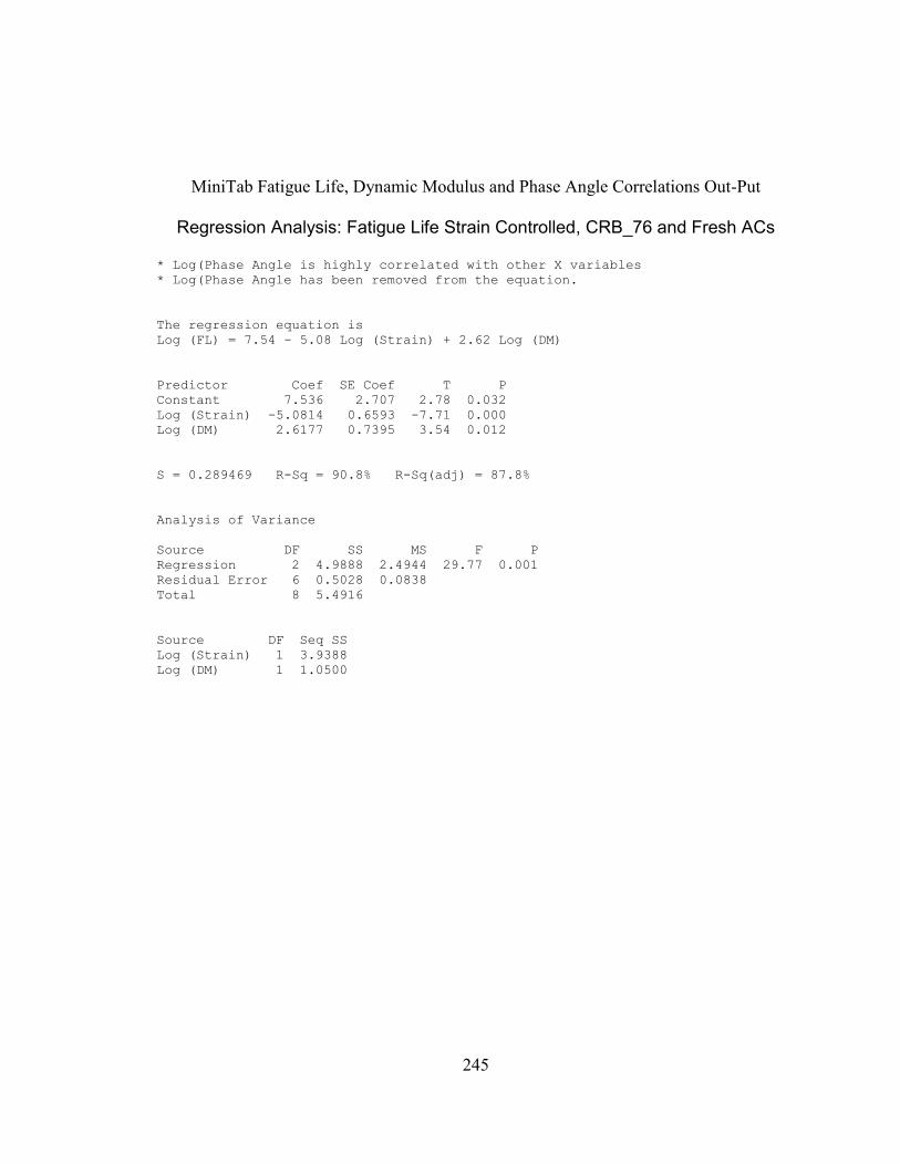
245
MiniTab Fatigue Life, Dynamic Modulus and Phase Angle Correlations Out-Put
Regression Analysis: Fatigue Life Strain Controlled, CRB_76 and Fresh ACs * Log(Phase Angle is highly correlated with other X variables
* Log(Phase Angle has been removed from the equation.
The regression equation is
Log (FL) = 7.54 - 5.08 Log (Strain) + 2.62 Log (DM)
Predictor Coef SE Coef T P
Constant 7.536 2.707 2.78 0.032
Log (Strain) -5.0814 0.6593 -7.71 0.000
Log (DM) 2.6177 0.7395 3.54 0.012
S = 0.289469 R-Sq = 90.8% R-Sq(adj) = 87.8%
Analysis of Variance
Source DF SS MS F P
Regression 2 4.9888 2.4944 29.77 0.001
Residual Error 6 0.5028 0.0838
Total 8 5.4916
Source DF Seq SS
Log (Strain) 1 3.9388
Log (DM) 1 1.0500
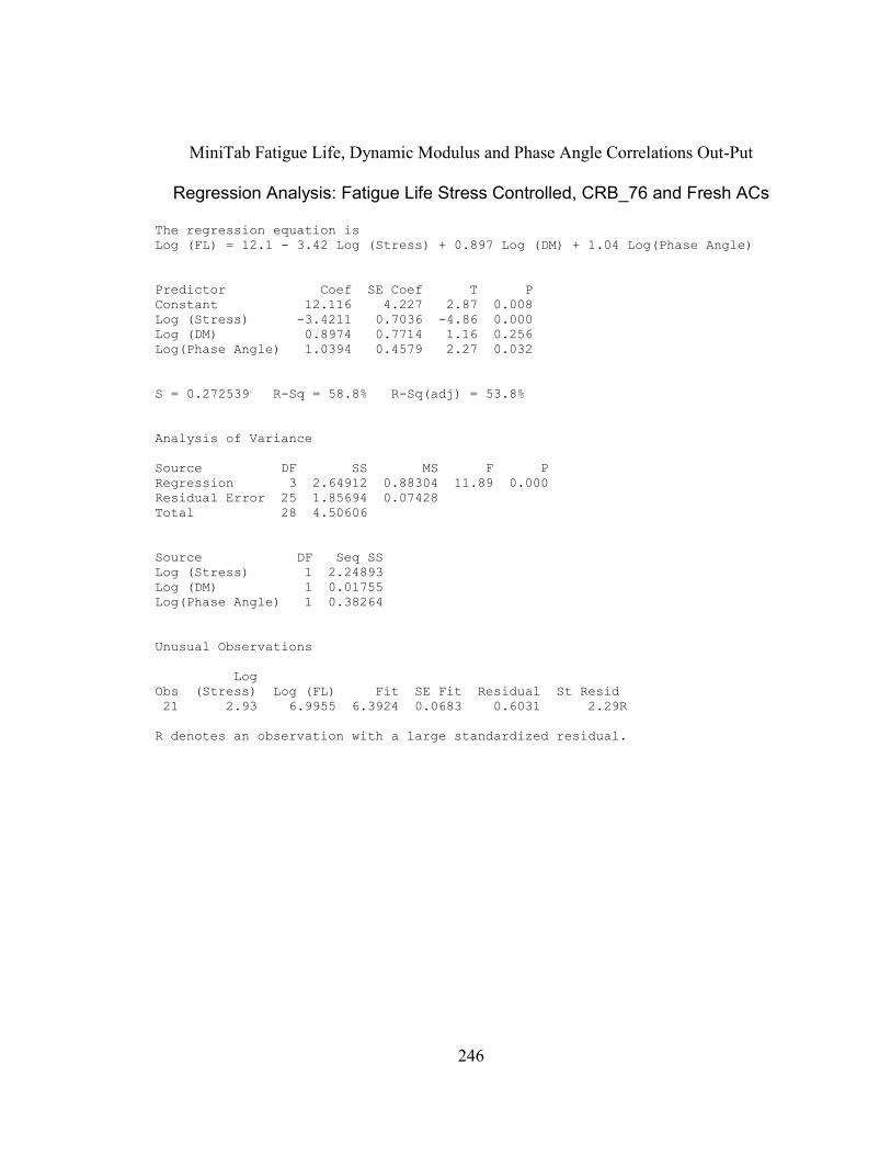
246
MiniTab Fatigue Life, Dynamic Modulus and Phase Angle Correlations Out-Put
Regression Analysis: Fatigue Life Stress Controlled, CRB_76 and Fresh ACs The regression equation is
Log (FL) = 12.1 - 3.42 Log (Stress) + 0.897 Log (DM) + 1.04 Log(Phase Angle)
Predictor Coef SE Coef T P
Constant 12.116 4.227 2.87 0.008
Log (Stress) -3.4211 0.7036 -4.86 0.000
Log (DM) 0.8974 0.7714 1.16 0.256
Log(Phase Angle) 1.0394 0.4579 2.27 0.032
S = 0.272539 R-Sq = 58.8% R-Sq(adj) = 53.8%
Analysis of Variance
Source DF SS MS F P
Regression 3 2.64912 0.88304 11.89 0.000
Residual Error 25 1.85694 0.07428
Total 28 4.50606
Source DF Seq SS
Log (Stress) 1 2.24893
Log (DM) 1 0.01755
Log(Phase Angle) 1 0.38264
Unusual Observations
Log
Obs (Stress) Log (FL) Fit SE Fit Residual St Resid
21 2.93 6.9955 6.3924 0.0683 0.6031 2.29R
R denotes an observation with a large standardized residual.
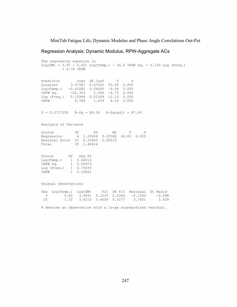
247
MiniTab Fatigue Life, Dynamic Modulus and Phase Angle Correlations Out-Put Regression Analysis: Dynamic Modulus, RPW-Aggregate ACs The regression equation is
Log(DM) = 3.97 - 0.421 Log(Temp.) - 26.4 %RPW Sq. + 0.130 Log (Freq.)
+ 6.78 %RPW
Predictor Coef SE Coef T P
Constant 3.97387 0.07420 53.56 0.000
Log(Temp.) -0.42082 0.04400 -9.56 0.000
%RPW Sq. -26.353 5.566 -4.73 0.000
Log (Freq.) 0.12966 0.01069 12.13 0.000
%RPW 6.784 1.479 4.59 0.000
S = 0.0717295 R-Sq = 89.3% R-Sq(adj) = 87.9%
Analysis of Variance
Source DF SS MS F P
Regression 4 1.33464 0.33366 64.85 0.000
Residual Error 31 0.15950 0.00515
Total 35 1.49414
Source DF Seq SS
Log(Temp.) 1 0.46014
%RPW Sq. 1 0.00973
Log (Freq.) 1 0.75655
%RPW 1 0.10822
Unusual Observations
Obs Log(Temp.) Log(DM) Fit SE Fit Residual St Resid
4 0.60 3.9941 4.1235 0.0364 -0.1294 -2.09R
25 1.32 3.6210 3.4609 0.0277 0.1601 2.42R
R denotes an observation with a large standardized residual.
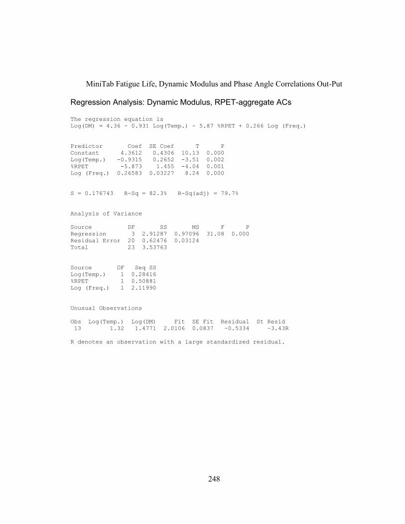
248
MiniTab Fatigue Life, Dynamic Modulus and Phase Angle Correlations Out-Put Regression Analysis: Dynamic Modulus, RPET-aggregate ACs The regression equation is
Log(DM) = 4.36 - 0.931 Log(Temp.) - 5.87 %RPET + 0.266 Log (Freq.)
Predictor Coef SE Coef T P
Constant 4.3612 0.4306 10.13 0.000
Log(Temp.) -0.9315 0.2652 -3.51 0.002
%RPET -5.873 1.455 -4.04 0.001
Log (Freq.) 0.26583 0.03227 8.24 0.000
S = 0.176743 R-Sq = 82.3% R-Sq(adj) = 79.7%
Analysis of Variance
Source DF SS MS F P
Regression 3 2.91287 0.97096 31.08 0.000
Residual Error 20 0.62476 0.03124
Total 23 3.53763
Source DF Seq SS
Log(Temp.) 1 0.28416
%RPET 1 0.50881
Log (Freq.) 1 2.11990
Unusual Observations
Obs Log(Temp.) Log(DM) Fit SE Fit Residual St Resid
13 1.32 1.4771 2.0106 0.0837 -0.5334 -3.43R
R denotes an observation with a large standardized residual.
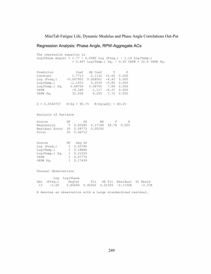
249
MiniTab Fatigue Life, Dynamic Modulus and Phase Angle Correlations Out-Put Regression Analysis: Phase Angle, RPW-Aggregate ACs The regression equation is
Log(Phase Angle) = 1.77 - 0.0680 Log (Freq.) - 1.19 Log(Temp.)
+ 0.687 Log(Temp.) Sq. - 9.35 %RPW + 32.4 %RPW Sq.
Predictor Coef SE Coef T P
Constant 1.7713 0.1132 15.65 0.000
Log (Freq.) -0.067955 0.008061 -8.43 0.000
Log(Temp.) -1.1933 0.2039 -5.85 0.000
Log(Temp.) Sq. 0.68706 0.08705 7.89 0.000
%RPW -9.349 1.117 -8.37 0.000
%RPW Sq. 32.438 4.200 7.72 0.000
S = 0.0540757 R-Sq = 90.7% R-Sq(adj) = 89.2%
Analysis of Variance
Source DF SS MS F P
Regression 5 0.85940 0.17188 58.78 0.000
Residual Error 30 0.08773 0.00292
Total 35 0.94713
Source DF Seq SS
Log (Freq.) 1 0.20780
Log(Temp.) 1 0.18886
Log(Temp.) Sq. 1 0.21059
%RPW 1 0.07776
%RPW Sq. 1 0.17439
Unusual Observations
Log Log(Phase
Obs (Freq.) Angle) Fit SE Fit Residual St Resid
13 -2.00 0.80494 0.92002 0.02393 -0.11508 -2.37R
R denotes an observation with a large standardized residual.
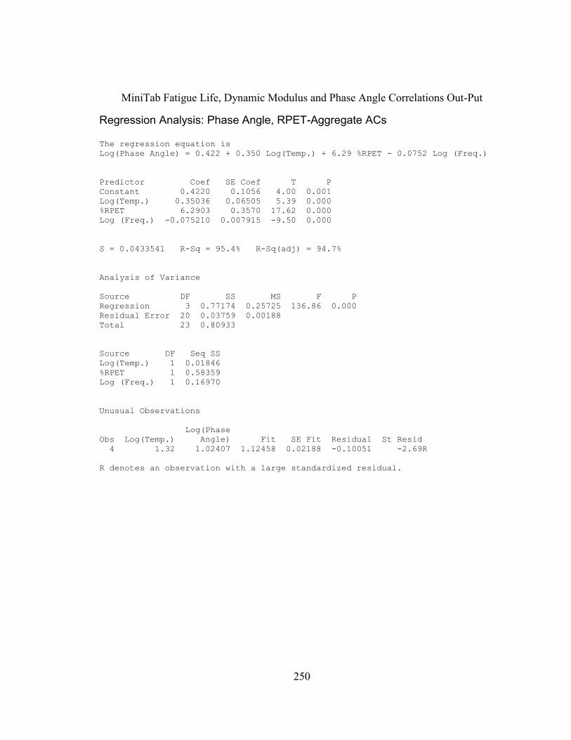
250
MiniTab Fatigue Life, Dynamic Modulus and Phase Angle Correlations Out-Put
Regression Analysis: Phase Angle, RPET-Aggregate ACs The regression equation is
Log(Phase Angle) = 0.422 + 0.350 Log(Temp.) + 6.29 %RPET - 0.0752 Log (Freq.)
Predictor Coef SE Coef T P
Constant 0.4220 0.1056 4.00 0.001
Log(Temp.) 0.35036 0.06505 5.39 0.000
%RPET 6.2903 0.3570 17.62 0.000
Log (Freq.) -0.075210 0.007915 -9.50 0.000
S = 0.0433541 R-Sq = 95.4% R-Sq(adj) = 94.7%
Analysis of Variance
Source DF SS MS F P
Regression 3 0.77174 0.25725 136.86 0.000
Residual Error 20 0.03759 0.00188
Total 23 0.80933
Source DF Seq SS
Log(Temp.) 1 0.01846
%RPET 1 0.58359
Log (Freq.) 1 0.16970
Unusual Observations
Log(Phase
Obs Log(Temp.) Angle) Fit SE Fit Residual St Resid
4 1.32 1.02407 1.12458 0.02188 -0.10051 -2.69R
R denotes an observation with a large standardized residual.
251
VITAE
NAME: Muhammad Abubakar Dalhat
NATIONALITY: Nigerian
HOME ADDRESS: No. 10, Sambo road, Tudun Jukun Zaria, Kaduna State, Nigeria.
POSTAL ADDRESS: P. o Box 1548, No. 10, Sambo road, Tudun Jukun Zaria,
Kaduna State, Nigeria.
EMAIL: [email protected]
EDUCATIONAL QUALIFICATIONS
Doctor of Philosophy in Civil Engineering (Pavement Material).
Feb. 2013 - Mar. 2017
King Fahd University of Petroleum and Minerals,
Dhahran, Saudi Arabia.
Master of Science in Civil Engineering (Transportation)
Feb. 2011 - Nov. 2012
King Fahd University of Petroleum and Minerals,
Dhahran, Saudi Arabia.
Bachelor of Engineering (Civil)
Jan. 2005 - Mar. 2010
Ahmadu Bello University,
Zaria, Nigeria.
Related Publications:
1. Al-Abdul Wahhab H.I. and Dalhat M.A., 2016. Storage Stability and High Temperature Performance of Recycled Plastic Modified Asphalt Binder. Road Material and Pavement Design. DIO: 10.1080/14680629.2016.1207554.
2. Dalhat M.A. and Al-Abdul Wahhab H.I., 2016. Cement-less and asphalt-less concrete bounded by recycled plastic. Construction and Building Materials. 119, 206–214
3. Dalhat M.A. and Al-Abdul Wahhab H.I., 2015. Performance of recycled plastic waste modified asphalt binder in Saudi Arabia. International Journal of Pavement Engineering, DOI: 10.1080/10298436.2015.1088150.
Relevant link: https://www.researchgate.net/profile/Muhammad_A_Dalhat/contributions
Related Documents