t ¯ t E T + jets FERMILAB-THESIS-2008-35

Welcome message from author
This document is posted to help you gain knowledge. Please leave a comment to let me know what you think about it! Share it to your friends and learn new things together.
Transcript

UNIVERSITA' DEGLI STUDI DITRENTO
Facoltá di Scienze Matematiche, Fisiche eNaturali
DOTTORATO DI RICERCA IN FISICA -CICLO XX
Tesi di Dottorato
Measurement of the tt productioncross section in the 6ET + jets
channel at CDF
Coordinatore:Prof. Renzo Vallauri
Supervisore:Prof. Ignazio Lazzizzera
Dottorando:Gabriele Compostella
6 Marzo 2008
FERMILAB-THESIS-2008-35


To M.4,my irreplaceable source
of true happiness...


Contents
Introduction 1
1 Theoretical Overview 3
1.1 The Standard Model of particle physics . . . . . . . . . . . . . . . . 31.1.1 Quantum Electrodynamics . . . . . . . . . . . . . . . . . . . 41.1.2 Electroweak Theory . . . . . . . . . . . . . . . . . . . . . . . 51.1.3 Quantum Chromo Dynamics . . . . . . . . . . . . . . . . . . 9
1.2 Physics beyond the Standard Model . . . . . . . . . . . . . . . . . . 101.3 The Top quark . . . . . . . . . . . . . . . . . . . . . . . . . . . . . 11
1.3.1 Top quark production . . . . . . . . . . . . . . . . . . . . . 121.3.2 Top quark decays . . . . . . . . . . . . . . . . . . . . . . . . 151.3.3 Top quark mass . . . . . . . . . . . . . . . . . . . . . . . . . 18
2 Tevatron Accelerator complex 23
2.1 Instantaneous and integrated Luminosity . . . . . . . . . . . . . . . 232.2 The proton source . . . . . . . . . . . . . . . . . . . . . . . . . . . . 252.3 The Main Injector . . . . . . . . . . . . . . . . . . . . . . . . . . . . 272.4 The antiproton source . . . . . . . . . . . . . . . . . . . . . . . . . 28
2.4.1 The Recycler ring . . . . . . . . . . . . . . . . . . . . . . . . 282.5 The Tevatron ring . . . . . . . . . . . . . . . . . . . . . . . . . . . . 29
3 The CDF Detector in Run II 35
3.1 CDF Coordinate systems . . . . . . . . . . . . . . . . . . . . . . . . 363.2 Tracking system . . . . . . . . . . . . . . . . . . . . . . . . . . . . . 37
3.2.1 Silicon vertex detector . . . . . . . . . . . . . . . . . . . . . 383.2.2 The COT . . . . . . . . . . . . . . . . . . . . . . . . . . . . 423.2.3 Time of �ight detector . . . . . . . . . . . . . . . . . . . . . 44
3.3 Calorimetric systems . . . . . . . . . . . . . . . . . . . . . . . . . . 453.3.1 The Central Calorimeter . . . . . . . . . . . . . . . . . . . . 453.3.2 The plug calorimeter . . . . . . . . . . . . . . . . . . . . . . 46
3.4 Muon detectors . . . . . . . . . . . . . . . . . . . . . . . . . . . . . 483.5 Cherenkov luminosity counters . . . . . . . . . . . . . . . . . . . . . 503.6 Forward Detectors . . . . . . . . . . . . . . . . . . . . . . . . . . . 513.7 Trigger and data acquisition system . . . . . . . . . . . . . . . . . . 52
3.7.1 Level 1 primitives . . . . . . . . . . . . . . . . . . . . . . . . 533.7.2 Level 2 primitives . . . . . . . . . . . . . . . . . . . . . . . . 543.7.3 Level 3 primitives . . . . . . . . . . . . . . . . . . . . . . . . 57

VI CONTENTS
3.7.4 Trigger Upgrades . . . . . . . . . . . . . . . . . . . . . . . . 573.8 O�ine data processing . . . . . . . . . . . . . . . . . . . . . . . . . 58
4 Reconstruction of Physical Objects 61
4.1 Track reconstruction . . . . . . . . . . . . . . . . . . . . . . . . . . 614.1.1 Outside-In tracking . . . . . . . . . . . . . . . . . . . . . . . 624.1.2 Inside-Out algorithm . . . . . . . . . . . . . . . . . . . . . . 63
4.2 Primary vertex reconstruction . . . . . . . . . . . . . . . . . . . . . 644.3 Jet reconstruction . . . . . . . . . . . . . . . . . . . . . . . . . . . . 65
4.3.1 Jet corrections . . . . . . . . . . . . . . . . . . . . . . . . . 684.4 Missing energy measurement . . . . . . . . . . . . . . . . . . . . . . 744.5 b-jet identi�cation . . . . . . . . . . . . . . . . . . . . . . . . . . . . 754.6 Electron identi�cation . . . . . . . . . . . . . . . . . . . . . . . . . 774.7 Muon reconstruction . . . . . . . . . . . . . . . . . . . . . . . . . . 784.8 Tau reconstruction . . . . . . . . . . . . . . . . . . . . . . . . . . . 784.9 Photon identi�cation . . . . . . . . . . . . . . . . . . . . . . . . . . 79
5 Neural Networks 83
5.1 Introduction . . . . . . . . . . . . . . . . . . . . . . . . . . . . . . . 835.2 Perceptrons and Neural Networks . . . . . . . . . . . . . . . . . . . 835.3 Training . . . . . . . . . . . . . . . . . . . . . . . . . . . . . . . . . 86
5.3.1 Reactive Taboo Search training algorithm . . . . . . . . . . 885.3.2 BFGS training algorithm . . . . . . . . . . . . . . . . . . . . 89
6 The tt→ 6ET + jets channel selection 93
6.1 Monte Carlo samples . . . . . . . . . . . . . . . . . . . . . . . . . . 936.2 Data . . . . . . . . . . . . . . . . . . . . . . . . . . . . . . . . . . . 946.3 6ET and 6ET signi�cance . . . . . . . . . . . . . . . . . . . . . . . . . 956.4 b-jet identi�cation e�ciency and scale factor . . . . . . . . . . . . . 986.5 Additional kinematical variables . . . . . . . . . . . . . . . . . . . . 1006.6 Event Prerequisites . . . . . . . . . . . . . . . . . . . . . . . . . . . 1026.7 Neural Network Training . . . . . . . . . . . . . . . . . . . . . . . . 1036.8 Background estimation . . . . . . . . . . . . . . . . . . . . . . . . . 1106.9 Positive b-tagging rate parameterization . . . . . . . . . . . . . . . 111
6.9.1 b-tagging rate parameterization . . . . . . . . . . . . . . . . 1126.9.2 b-tagging matrix . . . . . . . . . . . . . . . . . . . . . . . . 1156.9.3 b-tagging matrix checks . . . . . . . . . . . . . . . . . . . . . 117
6.10 Event selection . . . . . . . . . . . . . . . . . . . . . . . . . . . . . 1246.10.1 Optimization and Best Cut . . . . . . . . . . . . . . . . . . 124
7 Cross section measurement and systematic uncertainties 135
7.1 The �nal sample . . . . . . . . . . . . . . . . . . . . . . . . . . . . 1357.2 Systematics . . . . . . . . . . . . . . . . . . . . . . . . . . . . . . . 138
7.2.1 Background prediction systematic . . . . . . . . . . . . . . . 1387.2.2 Luminosity systematic . . . . . . . . . . . . . . . . . . . . . 1387.2.3 Monte Carlo generator dependent systematics . . . . . . . . 1387.2.4 PDF-related systematics . . . . . . . . . . . . . . . . . . . . 140

CONTENTS VII
7.2.5 ISR/FSR-related systematics . . . . . . . . . . . . . . . . . 1407.2.6 Systematics due to the jet energy response . . . . . . . . . . 1427.2.7 b-tagging scale factor systematics . . . . . . . . . . . . . . . 1447.2.8 Trigger systematics . . . . . . . . . . . . . . . . . . . . . . . 145
7.3 Cross section measurement . . . . . . . . . . . . . . . . . . . . . . . 146
Conclusions 151


Introduction
This thesis is focused on an inclusive search of the tt→ 6ET +jets decay channelby means of neural network tools in proton antiproton collisions at
√s = 1.96 TeV
recorded by the Collider Detector at Fermilab (CDF).At the Tevatron pp collider top quarks are mainly produced in pairs through
quark-antiquark annihilation and gluon-gluon fusion processes; in the StandardModel description, the top quark then decays to a W boson and a b quark almost100% of the times, so that its decay signatures are classi�ed according to the Wdecay modes. When only oneW decays leptonically, the tt event typically containsa charged lepton, missing transverse energy due to the presence of a neutrinoescaping from the detector, and four high transverse momentum jets, two of whichoriginate from b quarks.
In this thesis we describe a tt production cross section measurement whichuses data collected by a �multijet� trigger, and selects this kind of top decays byrequiring a high-PT neutrino signature and by using an optimized neural networkto discriminate top quark pair production from backgrounds.
In Chapter 1, a brief review of the Standard Model of particle physics will bediscussed, focusing on top quark properties and experimental signatures.
In Chapter 2 will be presented an overview of the Tevatron accelerator chainthat provides pp collisions at the center-of-mass energy of
√s = 1.96 TeV , and
proton and antiproton beams production procedure will be discussed.The CDF detector and its components and subsystems used for the study of
pp collisions provided by the Tevatron will be described in Chapter 3.Chapter 4 will detail the reconstruction procedures used in CDF to detect
physical objects exploiting the features of the di�erent detector subsystems.Chapter 5 will provide an overview of the main concepts regarding Arti�cial
Neural Networks, one of the most important tools we will use in the analysis.Chapter 6 will be devoted to the description of the main characteristics of the
tt→ 6ET + jets decay channel used to train our neural network to discriminate thetop pair production from background processes. We will discuss the event selectionmethod and the tecnique used for background prediction, that will rely on b-jetsidenti�cation rate parameterization.
Finally, Chapter 7 will provide a description of the �nal data sample and adetailed discussion of the systematic uncertainties before determining the crosssection measurement by means of a likelihood maximization.


Chapter 1
Theoretical Overview
Our present understanding of the fundamental constituents of matter and theirinteractions is expressed in a theory called the Standard Model. The StandardModel was developed during the 1960's and 70's and has been extensively testedexperimentally. Whenever a prediction for an experimental observable could bemade by the Model, excellent agreement with experiment was found. The Stan-dard Model integrates two gauge theories: Quantum Chromodynamics (QCD),describing the strong interactions, and the electroweak (EW) theory of Glashow,Weinberg and Salam, which uni�es the weak and the electromagnetic interactions.These are both quantum �eld theories, and therefore the Standard Model is con-sistent with both quantum mechanics and special relativity.
1.1 The Standard Model of particle physics
The Standard Model [1, 2, 3, 4] is a quantum �eld theory based on the gaugesymmetry group SU(3)C × SU(2)L × U(1)Y . The �rst gauge group SU(3)C isrelated to the description of the strong interactions which a�ect quarks only andare mediated by gluons. SU(3)C de�nes the Quantum Chromo Dynamics (QCD)theory. On the other hand, SU(2)L × U(1)Y is the underlying symmetry whichprovides a theoretical description of electromagnetic and weak interactions.
According to the Standard Model there are two families of elementary par-ticles (i.e. particles which do not have any internal structure): fermions (withspin 1/2) and bosons (with spin 1). Fermions are subject to interactions mediatedthrough the exchange of gauge bosons. There are 12 elementary fermions: the 6ones interacting by the electroweak force only are named leptons and the 6 onesinteracting by both the electroweak and the strong force are named quarks. Lep-tons and quarks are further organized into three families, called generations: foreach generation, particles have their corresponding anti-particles having the sameproperties as the partner particles but opposite charges (the charge of the particleis the quantum number that de�nes the coupling of the particle to the electroweakforce carriers).
The �rst generation comprises the electron e−, with electric charge Q = −1,its corresponding neutrino νe with Q = 0, and two types (conventionally named��avours�) of quarks, the up and down, and their corresponding antiparticles (e+,

4 Theoretical Overview
νe, u and d). The up and down quarks, denoted by u and d, carry fractionary elec-tric charges Qu = 2
3and Qd = −1
3respectively. In addition to the electric charge,
quarks also carry an additional quantum number related to strong interaction, thecolor, labeling the three degenerate indipendent state of the fundamental triplet(anti-triplet) of exact SU(3)C �color� simmetry in which quarks (anti-quarks) live.Since �colored� particles are not observed in nature, quarks must be con�ned intocolor-neutral composite particles, called hadrons, which are categorized as baryonsand mesons depending on their quark composition: baryons are basically consti-tuted by three �valence� quarks, like proton and neutron: p ∼ uud and n ∼ udd.On the other hand, mesons are composed by a quark-antiquark pair, for instancepions π+ ∼ ud and π− ∼ du.
Second and third generation particles have identical properties to �rst genera-tion ones, but di�erent masses.
Interactions are mediated by gauge particles: the carrier of the electromagneticforce is the photon γ, which is massless and chargeless. The weak force is mediatedby three massive vector bosons: W± and Z0, with charge Q = ±1 and 0 respec-tively. The strong force among quarks is mediated by the eight gluons gα, whichare an octet of adjoint representation in color space; each gluon is massless andchargeless and has the possibility of interacting with other gluons as well as withquarks. Gravitational interactions are not part of the Standard Model framework.A spin 2 graviton boson is supposed to be the carrier of the gravitational force buthas never been observed.
1.1.1 Quantum Electrodynamics
Elementary particles are spin-12fermions: in absence of gauge �elds their dy-
namics is described by the Dirac equation and the corresponding Lagrangian:
LDirac = Ψ(x)(i∂µγµ −m)Ψ(x) (1.1)
LDirac is invariant under the following global U(1) transformation, acting on the�elds and their derivatives:
Ψ → eiQθΨ Ψ → e−iQθΨ ∂µΨ → eiQθ∂µΨ (1.2)
It is possible to consider a local transformation of the same kind by allowing theparameter θ in Eq. 1.2 to have a dependence on the space-time point x; but bydoing so the invariance of the Lagrangian in Eq. 1.1 is lost.
We can restore the invariance under local U(1) transformations of the typeΨ → ΨeiQθ(x) if we introduce an additional boson �eld Aµ(x), a gauge vectorassociated to the photon, interacting with the �eld Ψ and whose transformationscompensate the non-invariant terms in the Lagrangian. In this way, the U(1) gaugeinvariant Lagrangian of Quantum Electrodynamic (qed) can be written as:
LQED = Ψ(x)(iDµγµ −m)Ψ(x)− 1
4Fµν(x)F
µν(x) (1.3)
where we introduced the so called covariant derivative Dµ, de�ned as follows:
DµΨ = (∂µ − ieQAµ)Ψ (1.4)

1.1 The Standard Model of particle physics 5
Figure 1.1: The three families of elementary particles in the Standard Model.
that contains the interaction term between the photon and fermions, and the �eldstrength tensor Fµν , de�ned by:
Fµν = ∂µAν − ∂νAµ (1.5)
in photon kinematical term of Eq. 1.3.
1.1.2 Electroweak Theory
The Electroweak theory uni�es the weak isospin non-Abelian group SU(2)L
acting on left-handed fermions and the weak hypercharge (Abelian) group U(1)Y
in SU(2)L×U(1)Y . Introducing the Pauli matrices σi with i = 1, 2, 3 we can writethe four generators of SU(2)L×U(1)Y as Ti = σi
2coming from SU(2)L and Y
2from
U(1)Y . The commutation relations of the four group generators are the following:
[Ti, Tj] = iεijkTk; [Ti, Y ] = 0; i, j, k = 1, 2, 3. (1.6)
Left-handed fermions are SU(2)L doublets:
fL → ei~T~θfL; fL =
(νL
eL
),
(uL
dL
), ... (1.7)
while right-handed fermions transform as singlets:
fR → fR; fR = eR, uR, dR, .... (1.8)

6 Theoretical Overview
Fermions T T 3 Q YνL 1/2 1/2 0 −1eL 1/2 −1/2 −1 −1eR 0 0 −1 −2uL 1/2 1/2 2/3 1/3dL 1/2 −1/2 −1/3 1/3uR 0 0 2/3 4/3dR 0 0 −1/3 −2/3
Table 1.1: Fermion quantum numbers for the �rst generation in the StandardModel.
Fermions quantum numbers coming from the two groups are related to eachother and to charge by the following equation:
Q = T3 +Y
2. (1.9)
The number of associated gauge bosons of the model is equal to the number ofthe symmetry group generators, so we have four bosons: W i
µ (i = 1, 2, 3) and Bµ,associated to SU(2)L and U(1)Y respectively.
In order to write the Lagrangian for the electroweak sector of the StandardModel we can follow the same procedure used previously for the Quantum Elec-trodynamics, building the model around the conservation of the weak isospin andweak hypercharge under local gauge transformations. We can thus change theSU(2)L × U(1)Y symmetry from global to local and replace the �eld derivativeswith their corresponding covariant derivatives. For a generic fermion �eld f , wecan de�ne the covariant derivative as follows:
Dµf =
(∂µ − ig ~T · ~Wµ − g′
Y
2Bµ
)f (1.10)
where g and g′ are the coupling constants associated to SU(2)L and U(1)Y , respec-tively.
Similarly to QED the electroweak Lagrangian includes kinetic terms for thegauge �elds:
L = −1
4W i
µνWµνi − 1
4BµνB
µν (1.11)
where the �eld strength tensors are de�ned as follows:
W iµν = ∂µW
iν − ∂νW
iµ + gεijkWµjWνk
Bµν = ∂µBν − ∂νBµ (1.12)
where i, j, k are indeces of vector components in the adjoint representation ofSU(2)L.
The gauge invariant interactions and the fermion kinematics are generated byf iDµγ
µf terms in the Lagrangian, while the physical gauge bosons �elds W±µ , Zµ

1.1 The Standard Model of particle physics 7
Figure 1.2: The Higgs potential, and a pictorial representation of the spontaneussymmetry breaking mechanism.
and Aµ can be obtained calculating the electroweak interaction eigenstates, thatare found to be:
W±µ =
W1µ ∓ iW2µ√2
Zµ = W3µ cos θ −Bµ sin θ
Aµ = W3µ sin θ +Bµ cos θ (1.13)
where θ is the weak mixing angle.The gauge invariance of the electroweak Lagrangian is complicated by the ob-
served non-zero mass of the physical gauge bosons �elds W± and Z0, carriers ofthe weak force. In fact mass terms like M2
WWµWµ, M2
ZZµZµ and m2
f ff cannotbe added to the derived Lagrangian, since they explicitly violate SU(2)L × U(1)Y
gauge invariance.A method called Higgs Mechanism, based on spontaneous symmetry breaking,
is then used to solve the mass generation problem and will be brie�y described.
Spontaneous symmetry breaking
The spontaneous symmetry breaking happens when the Lagrangian describingthe dynamics of a physical system has a symmetry that is not preserved by thesystem ground states.
Given a gauge theory based on a local invariance with respect to a symmetrygroup G, and beingH⊂G the symmetry group of the vacuum state, with dim(G) =N and dim(H) = M , the general formulation of the Goldstone theorem statesthat N −M massless bosons will be absorbed by N −M massive vector bosons.Therefore, in the SU(2)L × U(1)Y , where dim(G) = 4 and H = U(1)em, threevector bosons will realize the desired mass spectrum. This mechanism requiresthe introduction of the Higgs �eld, a doublet of complex �elds: three of its fourdegrees of freedom will be spent for the longitudinal polarization states of the
8 Theoretical Overview
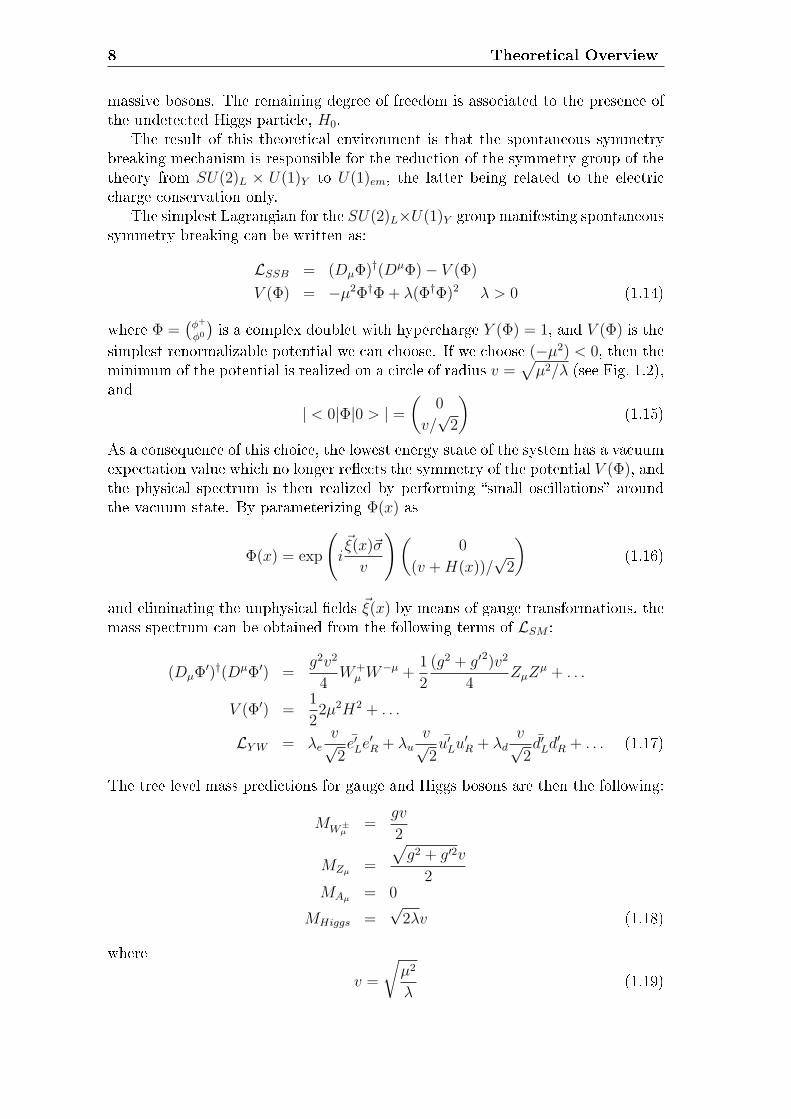
massive bosons. The remaining degree of freedom is associated to the presence ofthe undetected Higgs particle, H0.
The result of this theoretical environment is that the spontaneous symmetrybreaking mechanism is responsible for the reduction of the symmetry group of thetheory from SU(2)L × U(1)Y to U(1)em, the latter being related to the electriccharge conservation only.
The simplest Lagrangian for the SU(2)L×U(1)Y group manifesting spontaneoussymmetry breaking can be written as:
LSSB = (DµΦ)†(DµΦ)− V (Φ)
V (Φ) = −µ2Φ†Φ + λ(Φ†Φ)2 λ > 0 (1.14)
where Φ =(
φ+
φ0
)is a complex doublet with hypercharge Y (Φ) = 1, and V (Φ) is the
simplest renormalizable potential we can choose. If we choose (−µ2) < 0, then theminimum of the potential is realized on a circle of radius v =
√µ2/λ (see Fig. 1.2),
and
| < 0|Φ|0 > | =(
0
v/√
2
)(1.15)
As a consequence of this choice, the lowest energy state of the system has a vacuumexpectation value which no longer re�ects the symmetry of the potential V (Φ), andthe physical spectrum is then realized by performing �small oscillations� aroundthe vacuum state. By parameterizing Φ(x) as
Φ(x) = exp
(i~ξ(x)~σ
v
)(0
(v +H(x))/√
2
)(1.16)
and eliminating the unphysical �elds ~ξ(x) by means of gauge transformations, themass spectrum can be obtained from the following terms of LSM :
(DµΦ′)†(DµΦ′) =g2v2
4W+
µ W−µ +
1
2
(g2 + g′2)v2
4ZµZ
µ + . . .
V (Φ′) =1
22µ2H2 + . . .
LY W = λev√2e′Le
′R + λu
v√2u′Lu
′R + λd
v√2d′Ld
′R + . . . (1.17)
The tree level mass predictions for gauge and Higgs bosons are then the following:
MW±µ
=gv
2
MZµ =
√g2 + g′2v
2MAµ = 0
MHiggs =√
2λv (1.18)
where
v =
õ2
λ(1.19)

1.1 The Standard Model of particle physics 9
is determined from the muon decay: v = (√
2GF )−1/2 ∼ 246 GeV and �xes thescale of the spontaneous symmetry breaking.
This mechanism is called the Higgs mechanism and gives rise to mass termsfor W±, Z, as well as for quarks and leptons preserving the gauge invariance ofthe theory, at the cost of introducing a new scalar particle, not yet experimentallyobserved, the Higgs boson, whose mass and self-interaction are not theoreticallydetermined.
1.1.3 Quantum Chromo Dynamics
The gauge theory for strong interactions is based on SU(3)C , which is a nonAbelian Lie group generated by color transformations. The Quantum ChromoDynamics invariant Lagrangian can be built similarly to the qed one, with thedi�erence that the SU(3)C symmetry will require the color to be conserved. Sincethe gauge group is non Abelian, this will cause the bosons mediating the interac-tion, the gluons, to posses color charge and to interact among themselves as wellas with quarks.
Moreover, the additional gluon-gluon interactions cause the strong couplingconstant αS to have a qualitatively di�erent behaviour with the interaction mo-mentum transfer scale with respect to the QED coupling constant αQED.
We can introduce the qcd covariant derivative:
Dµq =
(∂µ − igs
λα
2Aα
µ
)q (1.20)
where
q =
q1q2q3
(1.21)
are the quark �elds, gs is the strong coupling constant, λα
2are SU(3) generators
given by 3× 3 traceless hermitian matrices, and Aαµ are gluon �elds, α = 1, ..., 8.
Then the qcd Lagrangian can be written as:
LQCD =∑
q
q(x)(iDµγµ −mq)q(x)−
1
4Fα
µνFµνα (1.22)
where the gluon �eld strength tensors are de�ned as follows:
Fαµν(x) = ∂µA
αν (x)− ∂νA
αµ(x) + gsf
αβγAµβAνγ (1.23)
and the related term in Eq. 1.22 provides three and four gluon interaction vertices.In expression 1.23, gS, the strong coupling constant (which is usually denoted
as αS =g2
S
4π), is found to decrease as the interaction energy scale increases, due to
vacuum polarization e�ects induced by gluon self-interactions:
αS(q2) =4π(
11− 23Nf (q2)
)ln(
−q2
Λ2QCD
) (1.24)

10 Theoretical Overview
In eq. 1.24, ΛQCD is the qcd energy scale, Nf (q2) is the number of quark �avours
that can be pair-produced at a given energy (i.e. the number of quark �avours withmq <
√−q2/2). The �running� of αS with energy allows the strong coupling to
be small enough at high energy, allowing a perturbative description of the strongforce. However, at small momentum transfer comparable with the mass of the lighthadrons, αS becomes of order unity and the perturbation approximation breaksdown. This large value of the coupling constant is the source of most mathematicalcomplications and uncertainties in QCD calculations at low energy. On the otherhand, it is of great importance that αS tends to zero in the high energy limit. Thisproperty gives rise to the so-called �asymptotic freedom�, and allows perturbationtheory to be used in theoretical calculations to produce experimentally veri�ablepredictions for hard scattering processes. At the same time the behaviour of thestrong coupling constant at low energy is responsible for quark con�nement intohadrons.
Trying to separate colored particles requires increasing energy density in thebinding color string, since the interaction potential grows linearly with the distancebetween the outgoing partons, until the creation of new color-singlet hadronic statesbecomes energetically favorable and energy is materialized into colored quark pairs.The fact that quarks are forced into color singlets yields �nal state color-neutralhadrons rather than free quarks and gluons. Thus a hard scattered parton evolvesinto a shower of partons and �nally into hadrons. This process is called partonshower evolution or hadronization.
1.2 Physics beyond the Standard Model
Recent developments show that the Standard Model of particle physics is in-complete and many issues still remain open, for example the recently proved nonzero masses of neutrinos, that would require an extension of the model.
Another problem, the so-called hierarchy problem concerns the corrections tothe Higgs mass: in fact the Higgs boson mass receives divergent quadratic radiativecorrections which need to be controlled by means of �ne-tuning cancellations in or-der to keep the mass at the electroweak energy scale �xed. Several ways of solvingthis issue have been explored, for example the hypothesis of new strong dynamicsthat could appear at the TeV scale (Technicolor theories). Another possible expla-nation allows the divergent corrections to mH to be cancelled by a new spectrumof particles at the electroweak scale: supersymmetric (SUSY) theories propose asupersymmetric partner for each SM particle with di�erent spin, solving the hier-archy problem by considering radiative corrections from supersymmetric partners.SUSY requires additional Higgs �elds in order to provide mass to fermions andtheir superpartners, for example in the minimal supersymmetric extension of SM,the MSSM, there are �ve Higgs bosons: h, H, A and H± which are associated totwo complex doublets.
Furthermore, Grand Uni�cation would require an extension of the StandardModel to include gravitational interactions in the theory.

1.3 The Top quark 11
1.3 The Top quark
The top quark was discovered during Run 1 of the Tevatron operation by cdfand dØ collaborations at Fermilab in 1995 [5, 6]. It was another success of theStandard Model, which had strongly predicted its existence.
Several experimental results and theoretical arguments already prior to the topquark discovery had provided evidence for its existence. These hints are mainlybased on theoretical self-consistency (namely the absence of anomalies), the ab-sence of �avour changing neutral currents (FCNC), and the measurement of weakisospin of the b-quark T3 = −1/2, thus demanding a T3 = 1/2 partner in its isospinmultiplet.
In 1964 Christenson and collaborators observed violation of CP symmetry inrare decays of neutral kaons at the Brookhaven National Laboratory [7].
To accomodate this result in the theory, in 1973, Kobayashi and Maskawaadded a phase factor eiδ into their quark mixing matrix [8]. At that time, onlythree quarks (u, d, s) were known. In their work they concluded that the only wayto have a renormalizable theory of weak interactions with CP violation was to intro-duce additional �elds, thus proposing the existence of three complete generationsof quarks, since the smallest unitary matrix which can exhibit a non removablecomplex phase is 3× 3 in size.
Afterwads, in 1974, at Brookhaven [9] and SLAC [10], two experiments inde-pendently observed a new resonance at 3.1 GeV/c2, the particle J/ψ, which wasimmediately interpreted as a cc bound state: this discovery of the charm-quarkcompleted the second generation of quarks.
Furthermore, one year later, in 1975, M. L. Perl and collaborators at SLACmade the �rst observation of the τ lepton [11], evidence for the existence of a thirdlepton and quark generation.
In 1977 the FNAL-E-0288 experiment collaboration at Fermilab discovered theb-quark (Υ = bb) [12]. The searches for a companion, the top quark, initiated im-mediately, based on the existence of the b and the empirically observed generationgrouping of the quarks and leptons previously discovered.
The quark model suggested that within any family fermions must appear in left-handed doublets and right-handed singlets of weak isospin [13]. So, in accordancewith the structure of the �rst generation, the left-handed b-quark was expectedto be part of a doublet of weak isospin (T 3
bL= −1/2), while the right-handed
b was associated to a isospin singlet: T 3bR
= 0. In the hypothesis that the t-quark did not exist, a b-quark would have appeared only as a singlet state: T 3
bL=
T 3bR
= 0. However the weak isospin of b-quarks was determined on the basis of themeasurement of the forward-backward asymmetry and of the total width of the bbproduction, by the JADE collaboration at DESY [14] and more recently from LEPexperiments [15], determining the b-quark to be part of a doublet of weak isospin.
Additionally, the experimentally determined absence of �avour changing neutralcurrents, an important feature of the Standard Model that excludes processes likeb→ µ+µ−X or b→ sX, where X is a state with no net �avour quantum numbers,implies that the b quark is a member of a SU(2) doublet.
Another compelling argument for the existence of the top quark follows from atheoretical consistency requirement. The renormalizability of the Standard Model

12 Theoretical Overview
demands the absence of triangle anomalies. Triangular fermion loops built-up byan axial-vector charge combined with two electric vector charges Q would breakthe renormalizability of the Standard Model. In order to avoid this from happeningit is su�cient to impose a constraint on the sum of the electric charges of all theleft-handed fermions: ∑
L
Q = 0 (1.25)
This condition is met in a complete standard generation in which the electric chargeof the leptons and those of the quarks of all color components add up to zero:∑
L
Q = −1 + 3×[(
+2
3
)+
(−1
3
)]= 0 (1.26)
The absence of the top quark in the third generation would violate the conditionof Eq. 1.25.
1.3.1 Top quark production
At hadron colliders top quarks are produced mainly in pairs through stronginteractions. Even if protons and antiprotons are not elementary particles, butcomposed of quarks and gluons, thanks to the asymptotic freedom property of qcdif the momenta of the initial particles are high enough (� ΛQCD ∼ 200 MeV ), wecan consider the interaction to take place between just two elementary particles(quarks or gluons), one in each incoming hadron, neglecting interactions amongthe other constituents of proton and antiproton.
The initial momentum of the interacting partons is however unknown, since agiven parton carries a fraction x of the proton (or antiproton) momentum accordingto a statistical distribution named �parton distribution function� (PDF). For eachparton type these functions describe the probability to �nd it with a momentumxP inside the proton [16], where P is the momentum of the proton (Fig. 1.3).The valence quarks (u and d) are most likely to carry a large fraction of theproton momentum, while gluons and sea quarks tend to carry smaller fractions.All allowed parton-parton interaction channels contribute to the experimental ttproduction cross section σtt to an amount depending on their distribution functionsin the primary hadrons, so in order to calculate it we must sum over all the possibleinteractions, weighted by their probability speci�ed by the PDF's. For proton-antiproton collisions:
σ(pp→ tt) =∑i,j
∫dzidzjfi/p(zi, µ
2)fj/p(zj, µ2)σ(ij → tt; s, µ2,Mtop) (1.27)
where the sum is over light quarks and gluons contained in the initial proton andantiproton, carrying momentum zi and zj of the initial hadron respectively; fi/p
and fj/p are the parton distribution functions for proton and antiproton respec-tively; σ is the parton-parton cross section. The center-of-mass energy of the i− jparton system is denoted by s and the parameter µ is a factorization scale which isintroduced to include resultant contributions from higher order Feynman diagrams.

1.3 The Top quark 13
Figure 1.3: Parton distribution functions of quarks and gluons in the proton attwo di�erent momentum transfers µ2 [16].
Figure 1.4: Leading order Feynman diagrams for tt production via strong interac-tion: (a) qq annihilation, (b) and (c) gg fusion.
At the Tevatron center-of-mass energy of√s = 1.96 TeV top quark pair pro-
duction occurs 85% of the times via quark-antiquark annihilation (qq) and for theremaining 15% via gluon fusion (gg). The leading order Feynman diagrams areshown in Fig. 1.4.
The theoretical Standard Model prediction for tt production at√s = 1.96 TeV ,
depends on the top mass valueMtop as shown in Fig. 1.5, and is σtt = 6.7+0.7−0.9 pb for
a top mass of 175 GeV/c2 [17, 18], meaning that, since the total pp inelastic crosssection is about 80 mbarn, we expect roughly one in 1010 collisions (≈ 7 · 10−4Hz

14 Theoretical Overview
Figure 1.5: Dependence of tt top pair production cross section on top quark mass.
rate) at Tevatron to produce a tt top quark pair, thus providing a real challengein the discrimination of the top events among a huge background.
The measurement of the production cross section for tt pairs can be a test forQCD, since a signi�cant deviation from the predicted value could indicate somekind of non Standard Model production mechanism. Fig. 1.6 shows some recentcross section measurements by CDF.
Single-top Production
Within the Standard Model, a single top quark can also be produced via elec-troweak interaction trough the following processes (see Fig. 1.7):
• t-channel: a space-like W boson (q2 ≤ 0) strikes a b quark in the proton sea,promoting it to a top quark; this channel is often referred to as W−gluonfusion, since the b quark arises from a gluon splitting to bb.
• s-channel: rotating the t-channel diagram so that the W boson becomestime-like (q2 ≥ (mt + m2
b)), single top production can happen trough qqannihilation.
• associated production: single top may be also produced via weak interactionin association with a real W boson (q2 = M2
W ); one of the initial partons isa b quark in the proton sea, as in the t-channel.
The cross sections for all these processes are proportional to the matrix element|Vtb|2 of the CKM matrix (see next section), therefore measuring the single topproduction cross section provides a direct probe of this SM parameter.

1.3 The Top quark 15
Figure 1.6: Cross section measurements by CDF compared with theoretical pre-dictions (shaded). This plot is updated to March 2007.
1.3.2 Top quark decays
In the Standard Model the top quark decay is mediated by the weak force,and its dominant decay signature is t → W+b or t → W−b with branching ratioBR(t→ Wb) ∼ 1. The additional decay channels t→ Wd and t→ Ws are allowedby the Standard Model but highly suppressed, thus giving minimal contribution,due to the very small values of the o�-diagonal elements in the quark �avour mix-ing matrix of weak eigenstates, the Cabibbo-Kobayashi-Maskawa (CKM ) matrix.CKM matrix arises because of the di�erence of mass and weak eigenstates forquarks, and can be expressed as a 3 × 3 unitary matrix operating on the charge−1/3 quark mass eigenstates (d, s and b) [16]:
VCKM
dsb
=
Vud Vus Vub
Vcd Vcs Vcb
Vtd Vts Vtb
dsb
≈
0.973 0.227 0.00390.021 0.972 0.0420.0081 0.041 0.999
dsb

16 Theoretical Overview
Figure 1.7: Leading order Feynman diagrams for electroweak production of singletop quarks: (a) s-channel, (b,c) t-channel and (d,e) associated production witha W .
The Standard Model predicts the top quark decay width to be [16]:
Γ(t→ Wb) =GFM
3top
8π√
2
(1− M2
W
M2top
)(1 + 2
M2W
M2top
)[1− 2αS
3π
(2π2
3− 5
2
)](1.28)
For Mtop = 175 GeV/c2 we have:
Γ(t→ Wb) ≈ 1, 55 GeV −→ τtop =1
Γtop
≈ 4 · 10−25 s (1.29)
This large width (Γtop � ΛQCD) causes the top quark to decay before hadronizing(its width is smaller then the characteristic hadronization time of QCD τhad ≈28 · 10−25 s), allowing its observation as a free particle. In particular, this featureenables precision mass measurements, otherwise impossible for the other quarksdue to non-perturbative e�ects in the hadronic bound state.
Thus to detect the top quark we just need to identify and reconstruct its decayproducts; consequently, the top pair decay signatures are classi�ed according to the

1.3 The Top quark 17
Figure 1.8: Pictorial view of tt top pair production at tree level by qq annihilationfollowed by the pair decay into the µ+ jets channel.
Channel Decay Mode Branching Ratio
All-hadronic tt→ qq′b qq′b 36/81Lepton+jets tt→ qq′b eνb 12/81
tt→ qq′b µνb 12/81tt→ qq′b eτ b 12/81
Di-lepton tt→ eνb eνb 1/81tt→ µνb µνb 1/81tt→ eνb µνb 2/81tt→ eνb τνb 2/81tt→ µνb τνb 2/81tt→ τνb τνb 1/81
Table 1.2: Standard Model tt decay modes and their associated relative branchingratios.
W decay modes. TheW bosons decay to either one of the three generation leptons,W+ → e+νe, W
+ → µ+νµ, W+ → τ+ντ , or into the lightest two generations of
quarks: W+ → ud, W+ → cs.
This gives rise to di�erent decay channels that produce di�erent experimental

18 Theoretical Overview
Figure 1.9: Standard Model tt decay signatures.
signatures in the detector. The di-lepton category represents the case in whichboth W bosons decay leptonically; this channel is somehow complicated by thetwo non-observable neutrinos in the �nal state, has the lowest branching ratio, butis the cleanest among the three, due to the clear signature of its two leptons. Mainbackground sources are di-boson and Drell-Yan events.
The lepton+jets signature on the other hand arises when one of the W decayshadronically and the other into lν; those involving τ 's are di�cult to isolate becauseof the poor tau signature.
Finally, the all-hadronic channel corresponds to the case in which both Wbosons decay into quarks; this channel has the largest branching ratio but su�ersfrom a large QCD background of multijet states.
The possible tt decay modes and their corresponding branching ratios are sum-marized in Tab. 1.2 and Fig. 1.9.
1.3.3 Top quark mass
The top quark mass Mtop, is an important parameter in di�erent areas of Par-ticle Physics. Its precise measurement is important to set basic parameters in thecalculation of the electroweak processes, and provides a constraint on the mass ofthe Higgs boson.
In fact, W mass theoretical calculation is subject to radiative corrections thatarise from creation and absorbtion of virtual quarks and bosons. Quark correctionsdepend on top mass while boson corrections depend on log(MH), where MH is theHiggs boson mass. Measuring with high precision W and top mass we can thusobtain a constraint on the mass of the Higgs. Fig. 1.10 shows the limits on Higgsmass that can be derived from direct and indirect measurement of top quark andW masses.
The current value of the top mass is set at 170.9±1.1 (stat) ±1.5 (syst) GeV/c2
(which corresponds to a total uncertainty of 1.8 GeV/c2) as a result of a combi-

1.3 The Top quark 19
Figure 1.10: Relationship between MW and Mtop as a function of the Higgs mass.Expectations for a number of H masses are shown within the shaded band. Avail-able EW data and Run 1 Tevatron measurements of MW and Mtop favour low MH
values. The small ellipse (1σ radius in the two observables) indicates the expectedconstraint by higher precision measurements of MW , Mtop at the end of Run 2.Results are from CDF, DØ, LEP and SLD.
nation of Tevatron Run I and Run II measurements [19], making it the heaviestknown elementary particle (see Fig. 1.11 for CDF results).

20 Theoretical Overview
Figure 1.11: Most recent CDF results using di�erent techniques and channels com-pared to the Tevatron average. Measurements in blue were included in the CDFcombination of March 2007.

Bibliography
[1] F. Mandl and G. Shaw, Quantum Field Theory, Wiley and Sons (1984).
[2] M. Peskin and D. Schroeder, An Introduction to Quantum Field Theory,HarperCollins (1995).
[3] C. Quigg, Gauge Theories of the Strong, Weak, and Electromagnetic
Interactions, Addison-Wesley (1997).
[4] S.F. Novaes, Standard Model: An Introduction, hep-ph/0001283.
[5] F. Abe et al. [CDF Collaboration], Evidence for top quark production in anti-pp collisions at
√s = 1.8 TeV, Phys. Rev. Lett. 73, (1994) 225.
[6] S. Abachi et al. [DØ Collaboration], Observation of the top quark,Phys. Rev. Lett. 74 (1995) 2632.
[7] J. H. Christenson et al., Evidence For The 2 Pi Decay Of The K(2)0 Meson,Phys. Rev. Lett. 13 (1964) 138.
[8] M. Kobayashi and T. Maskawa, CP Violation In The Renormalizable TheoryOf Weak Interaction, Prog. Theor. Phys. 49 (1973) 652.
[9] J. J. Aubert et al., Experimental Observation Of A Heavy Particle J,Phys. Rev. Lett. 33 (1974) 1404.
[10] J. E. Augustin et al., Discovery Of A Narrow Resonance In E+ E- Annihila-tion, Phys. Rev. Lett. 33 (1974) 1406.
[11] M. L. Perl et al., Evidence For Anomalous Lepton Production In E+ E- An-nihilation, Phys. Rev. Lett. 35 (1975) 1489.
[12] S. W. Herb et al., Observation Of A Dimuon Resonance At 9.5 GeV In400 GeV Proton - Nucleus Collisions, Phys. Rev. Lett. 39 (1977) 252.
[13] S. Weinberg, A Model Of Leptons, Phys. Rev. Lett. 19 (1967) 1264.
[14] W. Bartel et al., A Measurement Of The Electroweak Induced Charge Asym-metry In E+ E- → B Anti-B, Phys. Lett. B 146 (1984) 437.
[15] LEP collaborations, A combination of Preliminary LEP Electroweak Measure-ment and contraints on the Standard Model, CERN − PPE (1995) 95.

22 BIBLIOGRAPHY
[16] A. B. Balantekin et al. [Particle Data Group], Review of particle physics,J. Phys. G: Nucl. Part. Phys. 33 (2006).
[17] M. Cacciari et al., JHEP 0404:068 (2004).
[18] N. Kidonakis and R. Vogt, Phys. Rev. D 68 114014 (2003).
[19] Tevatron Electroweak Working Group [for the CDF and D0 Collaborations],A Combination of CDF and D0 Results on the Mass of the Top Quark, hep-ex/0703034, CDF Internal Note 8735, DØInternal Note 5378.

Chapter 2
Tevatron Accelerator complex
The Tevatron [1] is a proton-antiproton accelerator hosted at the Fermi NationalAccelerator Laboratory. With its center-of-mass energy of
√s = 1.96 TeV it is
the source of the highest energy pp collisions to date, up to now the only machinecapable of letting us examine dimensions up to 10−15 m, looking at the hadronconstituents, the quarks.
The Tevatron is the �nal and largest element of the Fermilab accelerator com-plex, illustrated in Fig. 2.1, and works primarily as a pp collider; however, it canalso accelerate a single proton beam and operate in �xed target mode to providea number of neutral and charged particle beams. The Tevatron collider obtainedthe �rst collisions in 1985, and during the course of its lifetime provided severalphysics runs, as listed in Tab. 2.1.
In the following, after spending a few words on one of the fundamental accel-erator parameters, the luminosity, a description of the acceleration apparatus willbe given.
2.1 Instantaneous and integrated Luminosity
While building an accelerator, a fundamental construction parameter is thedesign luminosity that needs to be achieved; in fact luminosity is a resource directlyrelated to the computation of the probability Wi→f for a generic process i → f ,where i and f are the initial and �nal states, respectively. In the case of Tevatron,the initial state is made up by two particles, a proton and an antiproton, while the�nal state is composed by a generic number N of particles. Taking into account theoverall four-momentum conservation, the probability amplitude for the p, p → fprocess has the following general structure:
〈f |T |p; p〉 = (2π)2δ(4)(Pf − pp − pp)〈Pf |M |pp; pp〉 (2.1)
where we made the following assumptions regarding each particle a in the initialand �nal states: a is described by a narrow wave packet that obeys, as obvious,the on-shell mass condition, the Klein-Gordon equation, and moreover, that ispeaked around a four-momentum pa, giving the following equation (were we hidedall remaining quantum numbers):
Fap (x) ≡ 〈x|a〉 =
1
(2π)3/2
∫d4q θ(q0)δ(q
2 −m2a)fp(q)e
−i qx (2.2)

24 Tevatron Accelerator complex
(a) (b)
Figure 2.1: (a): An airplane view of the Fermilab laboratory. The ring at thebottom of the �gure is the Main Injector, the above ring is the Tevatron. On theleft are clearly visible the paths of the external beamlines: the central beamline isfor neutral beams and the side beamlines are for charged beams (protons on theright, mesons on the left). (b): A sketch of the Fermilab accelerator chain.
Run Period Int. Lum. (pb−1)First Test 1997 0.025Run 0 1988-1989 4.5Run 1A 1992-1993 19Run 1B 1994-1995 90Run 1C 1995-1996 1.9Run 2A 2001-2004 400Run 2B 2004- >2000
Table 2.1: Integrated luminosity delivered by the Tevatron in its physics runs.Run2B is still in progress.
Integrating the square modulus of Eq. 2.1 over its space dependencies and afterother manipulations that use approximations allowed by the narrowness of thewave packets, assuming that protons and antiprotons are grouped in bunches, weend up with the following transition probability Wi→f :
Wi→f ≈ (2π)4δ4(Pf − pp − pp)|〈Pf |M |pp; pp〉|21
4ωpωp
∫d4x ρp(x)ρp(x) (2.3)
where ω's denote energies and ρ's, that have the meaning of probability density ofparticle location, are the time component of conserved four-currents given by:
i(F∗∂µF − F∂µF∗) (2.4)
The square amplitude in Eq. 2.3 is what can be computed by means of the StandardModel theory. What appears in the integral depends on the experimental setup;the integral itself has dimension of an inverse cross section and is a measure of the

2.2 The proton source 25
probability that incoming protons and antiprotons have to come in interaction. Wecan assume that the densities ρ are Gaussian near the collision points and that, forsimplicity, the collisions themselves are head-on; then, parameterizing the bunchespath by s and calling x(s)y(s) a plane orthogonal to the path in s, we can writeapproximately
ρ±(x(s), y(s), s± vt) =N±
(2π)3/2σxσyσs
exp
(− x2
2σ2x
− y2
2σ2y
− (s± vt)2
2σ2s
)(2.5)
where ± refers to proton/antiproton, N is the number of particles in a bunch, vis the speed of the bunches and σ's denote the radii of the portion of the crossingbunches that e�ectively overlap. In Eq. 2.3 we have consequently:∫
d4x ρp(x)ρp(x) ≡ ν∆
∫dx dy ds dtρp(x, y, s+ vt)ρp(x, y, s− vt)
= νNpNp
4πσxσy
∆
2v(2.6)
≡ L∆
2v
where ∆ is the whole lasting of the data taking, long with respect to the durationof each e�ective crossing of the colliding bunches, ν is the frequency of the crossingof the proton and anti-proton bunches, and (the lab reference frame is also thecenter of mass frame in our case)
v =|~p|ω, |~p| = |~pp| = |~pp|,
√m2
p + ~p2 = ω = ωp = ωp (2.7)
Thus we have
dWi→f
dt≈ δ4(Pf − pp − pp)
(2π)4
2ω|~p||〈f |M |pp; pp〉|2L
=(2π)4δ4(Pf − pp − pp)√
(pp · pp)2 −m2pm
2p
|〈f |M |pp; pp〉|2L
≡ σintL (2.8)
L is usually called (instantaneous) luminosity, while its integral over time L iscalled integrated luminosity. The bigger the luminosity, the bigger the probabilityto observe an interaction. For this reason the Tevatron has undergone a series ofimprovements during its lifetime in order to increase this fundamental parameter.Tab. 2.1 shows the luminosity served by the accelerator during its di�erent physicsruns.
2.2 The proton source
The process leading to pp collisions begins in a Cockroft-Walton generator (seeFig. 2.2) in which H− gas is produced by hydrogen ionization. H− ions are im-mediately accelerated by means of a multi step voltage divider up to an energy of

26 Tevatron Accelerator complex
Figure 2.2: The Cockroft-Walton generator, the starting point of the proton accel-eration chain.
Figure 2.3: Left: upstream view of the 400 MeV section of the Linac. Right: Teva-tron Superconducting Dipole Magnet.

2.3 The Main Injector 27
750 KeV and then transported through a transfer line to the linear accelerator,the Linac.
The second stage of the accelerator chain is a 150 meters long linear accelerator(see Fig. 2.3): the Linac [2, 3] picks up the H− ions at energy of 750 KeV , andaccelerates them up to the energy of 400 MeV inducing an oscillating electric �eldbetween a series of electrodes.
The Booster [4] takes the 400 MeV negative hydrogen ions from Linac, stripsthe electrons o�, which leaves only protons, and accelerates them up to 8 GeV .The Booster is the �rst circular accelerator in the Tevatron chain, and consists of aseries of magnets arranged around a 75-meter radius circle with 18 radio frequencycavities. The Booster loading scheme overlays the injected beam of negative H−
ions from the Linac with the one of H+ already circulating in the machine in orderto increase beam intensity; then the mixed beams go through a carbon foil, whichstrips o� the electrons turning the negative hydrogens into protons. When the bareprotons are collected in the Booster, they are accelerated to the energy of 8 GeVby the conventional method of varying the phase of RF �elds in the acceleratorcavities [1], and subsequently injected into the Main Injector. The �nal �batch�will contain a maximum of 5× 10¹² protons divided among 84 bunches spaced by18.9 ns, each consisting of 6× 10¹⁰ protons.
2.3 The Main Injector
The Main Injector [5] is a circular synchrotron with a 3 km circumference(seven times the circumference of the Booster) and plays a crucial role in linkingthe Fermilab acceleration facilities: the Main Injector can accelerate or decelerateparticles between the energies of 8GeV and 150GeV . The sources of these particlesand their �nal destination are variable, depending on the Main Injector operationmode: it can accept 8 GeV protons from the Booster, or 8 GeV antiprotons fromthe Recycler; it can accelerate protons up to 120 GeV for antiproton productionor deliver a proton beam to �xed target experiments. The beam energy, for bothproton and antiproton, can reach 150 GeV during the collider mode when particlesare injected to the Tevatron for the last stage of the acceleration. Furthermore,once Tevatron collisions end, the Main Injector can accept back the 150 GeVantiprotons in order to decelerate them down to 8 GeV before injecting them inthe Recycler.
The Linac accelerates protons to 400 MeV , and the Booster guides them upto 8 GeV . Afterwards the proton beam, through a transfer line, reaches the MainInjector where by means of radio frequency systems it is accelerated and bunched.
We can summarize the functions of the Main Injector as:
• Antiproton production: Providing beam to the antiproton production targetis one of the simplest tasks of the Main Injector. In this mode, a singlebatch of protons is accepted from the Booster, accelerated up to 120 GeVand extracted towards the target, which yields 8 GeV antiprotons.
• Fixed target modes : During �xed target operation, protons are acceleratedto the desired energy and then extracted to a stationary target, external to

28 Tevatron Accelerator complex
the ring. Extraction takes place from the Main Injector at 120 GeV . Thetarget can be anything from a sliver of metal to a �ask of liquid hydrogendepending on the experiment needs.
• Collider operations : in Collider Mode, in addition to supplying 120 GeV pro-tons for antiproton production, the Main Injector must also feed the Tevatronprotons and antiprotons at 150 GeV . The Main Injector maximum storedbeams are ∼ 3 · 1013 protons and ∼ 2 · 1012 antiprotons, beams are stored in36 bunches in the Tevatron. When the collision operation ends, another taskof the Main Injector is to recover antiprotons from the Tevatron, decelerateand then send them to the Recycler.
2.4 The antiproton source
The number of antiprotons available is an important limiting factor in produc-ing the high luminosity desired for Tevatron physics.
The Fermilab antiproton source [6] is comprised of a target station, two ringscalled the Debuncher and the Accumulator, and the transfer lines between theserings and the Main Injector.
Antiprotons p are produced from the 120 GeV proton beam extracted from theMain Injector and focused on a nikel target. Antiprotons are collected at 8 GeVwith wide acceptance around the forward direction, injected into the DebuncherRing, debunched into a continuous beam and stochastically cooled. The beam isthen transferred between cicles to the Accumulator were antiprotons are stored ata rate of about 25 · 1010 p/hour (improvements in the storage rate are still beingmade). Stacking within the accumulator acceptance is limited to a stored beam ofabout 1012 antiprotons.
When enough antiprotons have been accumulated in the Accumulator, theirtransfer starts. Antiproton beam destination can be either the Main Injector orthe Recycler ring (see Sec. 2.4.1).
Overall it can take from 10 to 20 hours to build up a stack of antiprotons, whichis then used in the Tevatron collisions. Antiproton availability is the most limitingfactor attaining high luminosities, so in this context it is important to mentionthe Recycler, the part of the acceleration chain designed to collect antiprotons leftat the end of a collider store, the period of time in which the colliding beams areretained in the Tevatron (roughly 20 hours).
2.4.1 The Recycler ring
The Recycler [7, 8] is a 3.3 Km long storage ring of �xed 8 GeV kinetic en-ergy, and is located directly above the Main Injector. It is composed primarily ofpermanent gradient magnets and quadrupoles. Three main tasks are designed forthe Recycler operations:
1. The most important feature of the Recycler is that it allows antiprotonsleft over at the end of Tevatron Collider stores to be re-cooled and re-used,allowing to recycle almost 75% of the antiprotons left after a store.

2.5 The Tevatron ring 29
Figure 2.4: Bunch structure of the Tevatron beams in Run 2.
2. It allows the Accumulator to operate optimally: since the antiproton produc-tion rate decreases as the beam current in the Accumulator ring increases,the Recycler is designed to act as a post-Accumulator cooler ring, being the�nal storage for 8 GeV antiprotons.
3. The usage of permanent magnets in the construction of the Recycler allowsto dramatically reduce the probability of unexpected losses of antiprotons.In fact, the ring has been designed so that Fermilab-wide power could be lostfor an hour with the antiproton beam surviving.
After a store has been circulating in the Tevatron for several hours, as particlesare gradually lost, the beam size slowly grows, and the luminosity degrades: adecision is then made to terminate the store and load a fresh one. To do so, sinceproton and antiproton orbits follow di�erent paths in the Tevatron, large chunksof metal are slowly moved into the proton beam until only the antiprotons areleft. At this point, antiprotons can be decelerated from 1 TeV to 150 GeV andthen transferred to the Main Injector. While the antiprotons are still circulatingat 150 GeV , they are decomposed back into fewer bunches (usually seven). Theantiprotons are then decelerated to 8 GeV and transferred to the Recycler ring.This procedure is repeated until no antiprotons from the store are left into theTevatron ring.
2.5 The Tevatron ring
The Tevatron [9] is the last stage of the Fermilab accelerator chain. The Teva-tron is a 1 km radius synchrotron able to accelerate the incoming 150 GeV beamsfrom Main Injector to 980 GeV , providing a center of mass energy of 1.96 TeV .The accelerator employs superconducting magnets (see Fig. 2.3) requiring cryo-genic cooling and consequently a large scale production and distribution of liquidhelium. During Run II the Tevatron operates at the 36× 36 bunches mode.
The antiprotons are injected after the protons have already been loaded. Whenthe Tevatron loading is complete, the beams are accelerated to the maximumenergy and collisions begin. The beam revolution time is 21 µs. The beams aresplit in 36 bunches organized in 3 trains each containing 12 bunches (see Fig. 2.4).Within a train the time spacing between bunches is 396 ns. An empty sector 139

30 Tevatron Accelerator complex
buckets long (2.6 µs) is provided in order to allow the kickers to raise to full powerand abort the full beam into a dump in a single turn. This is done at the endof a run or in case of an emergency. In the 36 × 36 mode, there are 72 regionsalong the ring where the bunch crossing occurs. While 70 of these are parasitic,in the vicinity of CDF and DØ detectors additional focusing and beam steeringis performed, to maximize the chance of a proton striking an antiproton. Thefocusing reduces the beam spot size and thus increases the luminosity, as seen inEq. 2.7 that shows how smaller values of σx, σy imply larger luminosity values.During collisions the instantaneous luminosity decreases in time as particles arelost and the beams begin to heat up. When the luminosity becomes too low toallow a signi�cant datataking (approximately after 15-20 hours) the current storeis dumped and a new cycle starts. A number of reasons can cause unwanted earlytermination of runs. Typical failures are a vacuum leak, a power supply failure ora magnet quench, a loss of magnet superconductivity in the ring.
Table 2.2 summarizes the accelerator parameters for Run II.
Parameter Value
Particles collided ppMaximum beam energy 0.980 TeVTime between collisions 0.396 µsCrossing angle 0 µradEnergy spread 0.14× 10⁻³
Bunch length 57 cmBeam radius 39µm for p, 31µm for pFilling time 30 minInjection energy 0.15 TeVParticles per bunch 2410 for p; 3× 10¹⁰ for pBunches per ring per species 36Average beam current 66µA for p, 8.2µA for pCircumference 6.12 Kmp source accumulation rate 13.5× 10¹⁰/hrMax number of p in accumulation ring 2.4× 10¹²
Table 2.2: Accelerator parameters for Run II con�guration [10].
Fig. 2.5 shows the Tevatron peak luminosity as a function of the time from thebeginning of Run II. The blue squares show the peak luminosity at the beginningof each store. The red triangle displays a point representing the last 20 peak valuesaveraged together.
Fig. 2.6 on the other hand shows the weekly and total integrated luminosity todate; while Fig. 2.7 shows the total luminosity delivered by the Tevatron comparedto the total luminosity recorded by the CDF experiment as a function of the storenumber.

2.5 The Tevatron ring 31
Figure 2.5: Run II peak luminosity.
Figure 2.6: Weekly and total integrated luminosity.

32 Tevatron Accelerator complex
Figure 2.7: Delivered and CDF acquired integrated luminosity as a function of theStore number.

Bibliography
[1] Fermilab Beams Division, Run II Handbook,http://www-ad.fnal.gov/runII/index.html.
[2] Fermilab Beams Division, Fermilab Linac Upgrade. Conceptual Design,FERMILAB-LU-Conceptual Design,http://lss.fnal.gov/archive/linac/fermilab-lu-999.shtml.
[3] Fermilab Beams Division, The Linac rookie book,http://www-bdnew.fnal.gov/operations/rookie_books/LINAC_v2.pdf.
[4] Fermilab Beams Division, The Booster rookie book,http://www-bdnew.fnal.gov/operations/rookie_books/Booster_V3_1.pdf.
[5] Fermilab Beams Division, The Main Injector rookie book,http://www-bdnew.fnal.gov/operations/rookie_books/Main_Injector_v1.pdf.
[6] Fermilab Beams Division, The Antiproton Source rookie book,http://www-bdnew.fnal.gov/operations/rookie_books/Pbar_V1_1.pdf.
[7] Fermilab Beams Division, The Recycler rookie book,http://www-bdnew.fnal.gov/operations/rookie_books/Recycler_RB_v1.pdf.
[8] G. Jackson, The Fermilab recycler ring technical design report. Rev. 1.2,FERMILAB-TM-1991 (1991).
[9] Fermilab Beams Division, The Tevatron rookie book,http://www-bdnew.fnal.gov/operations/rookie_books/Tevatron_v1.pdf.
[10] A. B. Balantekin et al. [Particle Data Group], Review of particle physics,J. Phys. G: Nucl. Part. Phys. 33 (2006).

34 BIBLIOGRAPHY

Chapter 3
The CDF Detector in Run II
This Chapter is dedicated to a detailed description of the CDF detector usedto study pp interactions provided by the Tevatron, and to a speci�c explanationof all the detector sub-systems, whose role is crucial for the reconstruction of thephysical objects needed for our analysis.
At the center of mass energy available at the Tevatron, proton-antiproton in-teractions are interpreted in terms of collisions between their constituents. Atthis level, the phenomenology is usually described in the framework of QuantumChromo Dynamics (QCD), as already highlighted in Chapter 1. At the end ofthe interaction process and after hadronization, collimated jets of particles emergefrom the scattering, whose energies and directions carry a reminiscence of initialpartons ones.
In the collisions, apart from QCD processes, electroweak production of W andZ bosons takes place as well. For that reason, aside the detection of collimatedspray of particles, the capability of detecting charged leptons and neutrinos asmissing energy is of great importance in the design of a particle detector.
The Collider Detector at Fermilab (CDF) is described below as con�gured forRun II; additional technical details covering all parts of the detector can be foundin CDF Technical Design Report [1] and in a series of guides for experimenters [2]and o�cial lectures [3].
A detector elevation view is presented in Fig. 3.1. The CDF architecture isquite common for this type of detectors: radially from the inside to the outside itfeatures a tracking system contained in a superconducting solenoid, calorimeters(electromagnetic and hadronic) and muon detectors. The whole CDF detectorweighs about 6000 tons.
CDF is located around one of the the two interaction points along the Tevatronring and has been designed in order to perform precise measurements of energy andmomentum of the jets and charged leptons produced by the pp collisions, as well asthe missing energy due to the neutrinos created inW and Z decays. Besides, it hasbeen studied to provide a �rst identi�cation of the produced particles, particularlyof the ones with relatively long lifetime coming from heavy quarks hadronization.
The reconstruction of an event begins with the identi�cation of jets performedby the calorimetry system. In order to determine the direction of the jet momenta,a precise measurement of the event interaction center is needed; moreover, the iden-ti�cation of the jets originated by heavy quarks requires an accurate reconstruction

36 The CDF Detector in Run II
Figure 3.1: Elevation view of the CDF II Detector.
of the secondary vertices produced in heavy �avour decays. These measurementstake advantage of the presence in the jets of charged particles, whose transversemomentum and trajectories can be reconstructed by a performant tracking systemsituated between the beam pipe and the calorimeter. Calorimetric and trackinginformations are also used to identify electrons produced in the event. Outside thecalorimeter, a complex of drift chambers for muon identi�cation is arranged. Muonsare very penetrating and leave a modest quantity of energy in the calorimeter: inorder to identify them, tracks with high transverse momentum are extrapolatedand matched to low energy calorimetric deposits and to stubs reconstructed in theexternal muon chambers.
In the following the structure of the detector CDF II will be examined in detail.
3.1 CDF Coordinate systems
CDF uses a Cartesian coordinate system centered in the nominal point of in-teraction, with the z axis coincident with the beamline and oriented parallel to themotion of the proton beam. The x axis is in the horizontal plane of the acceleratorring, pointing radially outward, while the y axis points vertically up (see Fig. 3.2).
For the simmetry of the detector, it is often convenient to work with cylindri-cal (z, r, φ) or polar (r, θ, φ) coordinates. The azimuthal angle φ is measured in thex− y plane starting from the x axis, and it is de�ned positive in the anti-clockwise

3.2 Tracking system 37
Figure 3.2: Isometric view of the CDF II Detector and its coordinate system.
direction; on the other side, the polar angle θ is measured from the positive di-rection of the z axis. The coordinate r de�nes the transverse distance from the zaxis. Another important coordinate that can be used instead of the polar angle θ,is called pseudorapidity and it is de�ned as:
η = − log tanθ
2(3.1)
The pseudorapidity is usually preferred to θ at hadron colliders, where events areboosted along the beamline, since it transforms linearly under Lorentz boosts, i.e.η intervals are invariant with respect to boosts. For these reasons, the detectorcomponents are chosen to be as uniformly segmented as possible along η and φcoordinates.
3.2 Tracking system
Charged particles passing through matter cause ionization typically localizednear the trajectory followed by the particle through the medium. Detecting ion-ization products gives geometrical information that can be used to reconstruct theparticle's path in the detector by means of the tracking procedure.
The inner part of CDF II is devoted to the tracking system, whose volume isimmersed in an uniform magnetic �eld of magnitude B = 1.4T , oriented along

38 The CDF Detector in Run II
Figure 3.3: The CDF II detector subsystems projected on the z/y plane.
the z-axis. The Lorentz force induced on charged particles constrains them to anhelicoidal trajectory, whose radius measured in the transverse plane x−y is directlyrelated to the particles transverse momentum PT (see 4.1 for details).
The CDF II tracking system is basically divided into an inner silicon strip de-tector aimed to provide a precise vertex determination, and an outer drift chamberfor momentum measurements. Fig. 3.3 shows the overall CDF II tracking volume,covering a pseudorapidity range up to |η| = 2.
3.2.1 Silicon vertex detector
The silicon vertex detector is crucial for precise determination of particle po-sitions, and in particular its information can be used to infer the presence in theevent of secondary decay vertices produced by heavy �avour decays.
The basic principle on which silicon strip detectors are based relies on the factthat a charged particle traveling across a silicon crystal produces electron-holepairs. In fact the fundamental characteristic of semiconductor materials, such assilicon, is the presence of a full valence band that is separated from the conductionband by an energy gap of only few eV .
When an electron is excited from the valence band to the conduction band,a positive �hole� is left in the valence band while the excited electron becomes anegative charge carrier in the conduction band.
By introducing impurities (doping) with a di�erent number of valence electrons,the number of available charge carriers in the semiconductor can be increased.
Doped semiconductors can be divided in two categories:

3.2 Tracking system 39
Figure 3.4: A generic silicon micro-strip detector.
1. n-type semiconductors, when the introduced impurity has one more valenceelectron than the silicon: the semiconductor will have additional electronsfor excitation into the conduction band.
2. p-type semiconductors, when the introduced impurity has one less valenceelectron than the silicon: the semiconductor has an excess of �holes� as chargecarriers in the valence band.
When one n-type semiconductor and one p-type semiconductor are placed together,the resulting device, called n−p junction, has some very special properties. Due tothe fact that each semiconductor contains charge carriers of di�ering polarity, thenegative electrons in the n-type semiconductor will be drawn towards the positiveholes in the p-type semiconductor and viceversa. After the equilibrium is reached,the n-type side possesses a net positive charge and the p-type side possesses a netnegative charge: an electrical potential barrier is created and a depletion regionarises between the n-type and p-type regions. For the silicon, the size of thisdepletion region is typically 10 µm and the potential through the junction is 0.6 eV .For each µm of depletion region traversed by an ionizing particle typically 100electron-hole pairs are produced, whose identi�cation becomes easier as the size ofthe depletion region increases; that's why the size of the depletion region is thusincreased applying external electric voltages to the p−n junction (reverse-biasing).This results in a larger sensitivity in detecting the ionization signals produced byincoming charged particles.
In a typical silicon micro-strip detector (Fig. 3.4), �nely spaced strips of stronglydoped p-type silicon (p+) are implanted on a lightly doped n-type silicon sub-strate (n−) ∼ 300 µm thick. On the opposite side, with respect to the p-type sil-icon implantation, a thin layer of strongly doped n-type silicon (n+) is deposited.A positive voltage applied to the n+ side depletes the n− volume of free electrons

40 The CDF Detector in Run II
(a) r−φ view of SVX II. (b) Perspective view of SVX II.
Figure 3.5: CDF II Silicon Vertex Detector.
Layer Radius [cm] # of strips Strip pitch [µm] Stereo Ladder [mm]stereo r - phi stereo r - φ stereo r - φ angle width length
0 2.55 3.00 256 256 60 141 90◦ 15.30 4× 72.431 4.12 4.57 576 384 62 125.5 90◦ 23.75 4× 72.432 6.52 7.02 640 640 60 60 +1.2◦ 38.34 4× 72.433 8.22 8.72 512 768 60 141 90◦ 46.02 4× 72.434 10.10 10.65 896 896 65 65 -1.2◦ 58.18 4× 72.43
Table 3.1: SVX summary.
and creates an electric �eld. When a charged particle crosses the active volume itcreates a trail of electron-hole pairs from ionization and the presence of the electric�eld drifts the holes to the p+ implanted strips producing a well localized signal.Usually the signal is collected by a cluster of strips, rather than being concentratedin just one strip. This allows to calculate the crossing point of the particle witha precision greater than the strip spacing, by weighting the strip positions by theamount of charge collected by each strip. With this method the Silicon Vertex De-tector installed by CDF collaboration can achieve individual hit position accuracyof 12 µm.
The CDF II Silicon VerteX Detector is shown in Fig. 3.5(a) and 3.5(b), and it isknown as SVX II [1]. It is composed of three di�erent barrels each 29 cm long, eachbarrel supporting �ve layers of double-sided silicon micro-strip detectors between2.5 and 10.7 cm from the beamline. The layers are numbered from 0 (innermost)to 4 (outermost); layers 0, 1 and 3 have wires parallel to the beam axis on oneside (axial strips for r - φ measurement) and tilted by 90◦on the other side (stereostrips for r - z measurement); layers 2 and 4 have axial strips on one side and stereostrips tilted by a small angle (1.2◦) on the other (Tab. 3.1).
To reach better performances in terms of resolution and tracking coverage, two

3.2 Tracking system 41
Figure 3.6: Left: cutaway transverse to the beam of the three subsystems of thesilicon vertex system. Right: sketch of the silicon detector in a z/y projectionshowing the η coverage of each layer.
special sub-detectors are added to the silicon tracker: the Layer 00 (L00) [4, 5] andthe Intermediate Silicon Layer (ISL), as illustrated in Fig. 3.6.
• L00: L00 is composed of a set of silicon strips assembled directly onto thebeam pipe (Fig. 3.7(a)). This device has six narrow and six wide groups ofladder in φ at radii 1.35 and 1.62 cm respectively, providing 128 read outchannels for the narrow groups and 256 channels for the wide groups. Thesilicon wafers are mounted on a carbon-�ber support which also providescooling. L00 sensors are made of light-weight radiation-hard single-sidedsilicon (di�erent from the ones used within SVX). Being so close to the beam,L00 allows to reach a resolution of ∼ 25/30 µm on the impact parameter oftracks of moderate pT , providing a powerful help to signal long-lived hadronscontaining a b quark. L00 allows to overcome the e�ects of multiple scatteringfor tracks passing through high density regions of SVX thus making it possibleto improve vertexing resolution.
• ISL: The Intermediate Silicon Layers (ISL) consist of double-sided siliconcrystals: one side has axial microstrips to provide measurements in the r-φplane, while the other one supplies z information by means of stereo strips.The arrangement of this device, shown in Fig. 3.7(b), varies according to theη range: in the central region (|η| < 1) it consists of a single layer placedat ∼ 22 cm from the beam line, while for 1 < |η| < 2 ISL is made of twolayers placed at r = 20 and 29 cm respectively (see Fig. 3.3). The twolayers at 1 < |η| < 2 are important to help tracking in a region where theCOT coverage is incomplete. In both regions, the stereo sampling enablesa full three-dimensional stand-alone silicon tracking. The ISL is intendedto improve the tracking resolution in the central region, while in the 1.0 <

42 The CDF Detector in Run II
(a) Transverse view of Layer 00, the innermostsilicon layer.
(b) Perspective view of ISL.
Figure 3.7: Layer 00 and ISL.
|η| < 2.0 region it provides a useful tool for silicon stand alone tracking inconjunction with SVX layers.
3.2.2 The COT
In addition to the silicon detector, the Central Outer Tracker (COT) [1] islocated at larger radii, and is used both to improve the momentum resolution andto provide useful informations to the trigger system.
This system is installed in the region |z| < 155 cm and between the radii of 43and 133 cm.
The COT is a cylindrical multi-wire open-cell drift chamber with a mixture of50:35:15 Ar-Ethane-CF4 gas used as active medium. The COT contains 96 sensewire layers, which are radially grouped into eight �superlayers� (see Fig. 3.8). Eachsuperlayer is divided in φ �supercells�, and each supercell has 12 sense wires andit is designed so that the maximum drift distance is approximately the same forall supercells. Therefore, the number of supercells in a given superlayer scalesapproximately with the radius of the superlayer. Half of the 30,240 sense wireswithin the COT run along the z direction (�axial�), while the others are installedat a small angle (2◦) with respect to the z direction (�stereo�).
A charged particle passing through the gas mixture leaves a trail of ionizationelectrons. These electrons are carried towards sense wires of the corresponding cell.The electron drift direction is not aligned with the electric �eld, being a�ected bythe 1.4 T magnetic �eld provided by the solenoid. Thus electrons originally atrest move in the plane perpendicular to the magnetic �eld forming an angle αwith respect to the electric �eld lines. The value of α, the so-called Lorentz angle,depends on the magnitude of both �elds and on the properties of the gas mixture.In the COT α ' 35◦(see Fig. 3.9).

3.2 Tracking system 43
Figure 3.8: COT section: the eight superlayers (left) and the alternation of �eldplates and wire plates (right).
Figure 3.9: Cross-sectional view of some COT cells. The radial direction in thepicture is horizontal and the angle between wire plane of the central cell and theradial direction is α ' 35◦.
The optimal situation in terms of resolution power is realized when the driftdirection is perpendicular to that of the track. Usually the optimization is donefor high PT tracks, which are almost radial. As a result, all COT cells are tilted35◦away from the radial direction, so that the ionization electrons drift in the φdirection. When the electrons get near the sense wire, the local 1
relectric �eld
accelerates them causing further ionization. The r - φ position of the track with

44 The CDF Detector in Run II
Figure 3.10: Time of Flight detector position.
respect to the sense wire is inferred by the signal arrival time.
A measurement of COT performance is given by the single hit position res-olution and has been measured to be about 140 µm, which translates into thetransverse momentum resolution δpT
pT∼0.15% pT
GeV/c.
3.2.3 Time of �ight detector
The Time of Flight system (TOF) [4, 6] is a Run II upgrade to the CDF detectorand it expands the particle identi�cation capability of CDF II in the low PT region.The TOF consists of 216 scintillator bars installed at a radial distance of about138 cm from the z axis in the 4.7 cm space between the outer shell of the COT andthe superconducting solenoid (see Figure 3.10). Bars are approximately 279 cmlong and 4 × 4 cm2 in cross-section. With its cylindrical geometry TOF provides2π coverage in φ, and covers the pseudorapidity range |η| < 1.0. Scintillator barsare read out at both ends by photomultiplier tubes, capable of providing adequategain even if used inside the 1.4 T magnetic �eld. The TOF detector measuresthe arrival time t of a particle with respect to the collision time t0. The massm of a particle traversing the device is determined using the path length L andmomentum P measured by the tracking system via the relationship
m =P
c
√(ct)2
L2− 1 (3.2)
A resolution of ∼ 110 ps has been achieved which allows a 2σ separation ofkaons from pions up to ∼ 1.6 GeV at |η| < 1.

3.3 Calorimetric systems 45
Figure 3.11: Geometry, parameters and performance summary of CDF Calorimet-ric System. The position resolution is given in r · φ× z cm2 and is measured for a50 GeV incident particle.
3.3 Calorimetric systems
The CDF II calorimetry system has been designed to measure energy and di-rection of neutral and charged particles leaving the tracking region. In particular,it is devoted to jet reconstruction as well as used to measure the missing transverseenergy associated to neutrino production.
Particles hitting the calorimeter can be divided in two classes according to theirinteraction with matter: electromagnetically interacting particles, such as electronsand photons, and hadronically interacting particles, such as mesons or baryonsproduced in hadronization processes. To detect these two classes of particles, twodi�erent calorimetric parts have been developed: an inner electromagnetic and anouter hadronic section, providing coverage up to |η| < 3.6. The calorimeter is alsosegmented in η−φ sections, called towers, projected towards the geometrical centerof the detector, in order to supply information on particle positions. Each towerconsists of alternating layers of passive material and scintillator tiles. The signalis read out via wavelength shifters (WLS) embedded in the scintillator and lightfrom WLS is then carried by light guides to photomultiplier tubes.
The calorimetric system is subdivided into three regions, central, wall and plug,in order of increasing pseudorapidity ranges, with the following naming convention:Central Electromagnetic (CEM), Central Hadronic (CHA), Wall Hadronic (WHA),Plug Electromagnetic (PEM) and Plug Hadronic (PHA); an inner commented viewof the detector is shown in Fig. 3.12. Table in Fig. 3.11 summarizes the mostimportant characteristics of each part of the calorimeter.
3.3.1 The Central Calorimeter
The Central Electro-Magnetic calorimeter (CEM) [1] is segmented in ∆η ×∆φ=0.11×15◦ projective towers consisting of alternate layers of lead and scintil-lator, while the Central and End Wall Hadronic calorimeters (CHA and WHArespectively), whose geometric tower segmentation matches the CEM one, use ironlayers as radiators. A perspective view of a central electromagnetic calorimetermodule, a wedge, is shown in Figure 3.13.

46 The CDF Detector in Run II
Figure 3.12: Schematic view of the inner parts of CDF detector.
Two position detectors are embedded in each wedge of the CEM:
• The Central Electromagnetic Strip chamber (CES) (see Fig. 3.14) is a two-dimensional strip/wire chamber located at the radial distance 184 cm. Itmeasures the charge deposition of the electromagnetic showers, providinginformation on their pulse-height and position with a �ner azimuthal seg-mentation than the calorimeter towers. This results in an increased purityof electromagnetic object reconstruction.
• The Central Pre-Radiator (CPR) consists of two wire chamber modulesplaced immediately in front of the calorimeter. It acts as pre-shower detectorand with its 3072 channels collects charge deposit by showers originated byinteraction of particles with tracking system and solenoid material. It canhelp in discriminating pions from electron and photons, because the latterdeposit a greater amount of energy in the chamber.
3.3.2 The plug calorimeter
The plug calorimeter, shown in Fig. 3.15, covers the η region from 1.1 to 3.6.Both electromagnetic and hadronic sectors are divided in 12 concentric η regions,with ∆η ranging from 0.10 to 0.64 according to increasing pseudorapidity, eachsegmented in 48 or 24 (for |η| < 2.1 or |η| > 2.1 respectively) projective towers.
As in the central calorimeter, there is a front electromagnetic compartment anda rear hadronic compartment (PEM and PHA). Projective towers consist of alter-nating layers of absorbing material (lead and iron for electromagnetic and hadronic

3.3 Calorimetric systems 47
Figure 3.13: Perspective view of a CEM module.
Figure 3.14: The CES detector in CEM. The cathode strips run in the x directionand the anode wires run in the z direction providing x and (r · φ) measurements.
sectors respectively) and scintillator tiles. The �rst layer of the electromagneticcalorimeter acts as a pre-shower detector; to this scope, the �rst scintillator tile is

48 The CDF Detector in Run II
Figure 3.15: Plug Calorimeter (PEM and PHA) inserted in the Hadron End Wallcalorimeter WHA and into the solenoid.
thicker (10 mm instead of 6 mm) and made of a brighter material.
As in the central calorimeter, a shower maximum detector (SMD) is also in-cluded in the plug electromagnetic calorimeter (PES). The PES consists of two lay-ers of 200 scintillating bars each, oriented at crossed relative angles of 45o (±22.5o
with respect to the radial direction). The position of a shower on the transverseplane is measured with a resolution of ∼ 1 mm.
3.4 Muon detectors
Muons are highly penetrating, so they are separated from charged hadrons bythe calorimeter, that acts as a shield for strongly and electromagnetic interactingparticles.
Muon identi�cation can then be performed by extrapolating the tracks outsidethe calorimeter and matching them to tracks segments (called stubs) reconstructedin an external muon detector.Figure 3.16 provides an overview of the muon detectors coverage, that goes up to|η| < 2.0. Muon systems are divided in muon chambers and muon scintillators, seeFig. 3.17:
• Central MUon detector (CMU) consists of a set of 144 modules, each contain-ing four layers of rectangular drift cells, operating in proportional mode. It

3.4 Muon detectors 49
Figure 3.16: η − φ coverage of the Run II muon detector system. The shape isirregular because of the obstruction by systems such as cryo pipes or structuralelements.
is placed immediately outside the calorimeter and supplies a global coverageup to |η| <0.6.
• Central Muon uPgrade (CMP) consists of four layers of single-wire propor-tional drift tubes stagged by half cell per layer and shielded by an additional60 cm steel layer. It is arranged in a square box around the CMU, providinga φ-dependent η coverage (see Figure 3.16).
• Central Scintillator uPgrade (CSP) is a layer of rectangular scintillator coun-ters placed on the outer surface of CMP.
• Central Muon eXtension (CMX) consists of a stack of eight proportional drifttubes, arranged in conical sections to extend the CMU/CMP coverage in the0.6 < |η| <1 region.
• Central Scintillator eXtension (CSX) consists of a layer of scintillator counterson both side of CMX. Thanks to scintillator timing, this device completeswith z information the measurement of the muon position provided by CMX(φ).
• Intermediate MUon detector (IMU) consists of four staggered layers of pro-portional drift tubes and two layers of scintillator tiles, arranged as for the

50 The CDF Detector in Run II
Figure 3.17: Schematic view of the whole CDF detector.
CMP/CSP system to extend triggering and identi�cation of muons up to|η| ≤ 1.5 and |η| ≤ 2, respectively.
3.5 Cherenkov luminosity counters
CDF measures the collider luminosity with a coincidence between two arrays ofCherenkov counters, the CLC, placed around the beam pipes on the two detectorsides [7]. The counters measure the average number of interactions per bunchcrossing µ, which is used to provide a measurement of the instantaneous luminosityL, by means of the following relation:
µ · fbc = σpp · L, (3.3)
where σpp is the total pp cross section at√s = 1.96 TeV (σpp = 60.7 ± 2.4 mb)
and fbc is the bunch crossing rate in the Tevatron. This method measures theluminosity with about the 6% systematic uncertainty. Each CLC module contains48 gas Cherenkov counters of conical shape projecting to the nominal interactionpoint, organized in concentric layers. It utilizes Cherenkov radiation: particlestraversing a medium at a speed higher than the speed of the light in the mediumradiate light into a cone around the particle direction; the cone opening angledepends on the ratio of the two speeds and the refraction index of the medium.Taking into account that light produced by any particle originated at the collisionpoint is collected with much higher e�ciency than for background stray particles,the CLC signal is thus approximately proportional to the number of traversingparticles produced in the collision.

3.6 Forward Detectors 51
Figure 3.18: Schematic view of the luminosity monitor inside a quadrant of CDF.
3.6 Forward Detectors
CDF Forward Detectors (see scheme in Fig. 3.19) include the Roman Pots de-tectors (RPS), beam shower counters (BSC) and two forward Mini Plug Calorime-ters (MP). These detectors enhance CDF sensitivity to production processes wherethe primary beam particles scatter inelastically in large impact parameter interac-tions.
The Tevatron complex allowed to arrange a proper spectrometer making useof the Tevatron bending magnets only on the antiproton side. On this side, atappropriate locations, scintillating �ber hodoscopes inside three RPS measure themomentum of the inelastically scattered antiproton. Only the direction of thescattered proton is measured on the opposite side. The BSC counters at 5.5 <|η| < 7.5 measure the rate of charged particles around the scattered primaries.
The MiniPlugs calorimeters at 3.5 < |η| < 5.1 measure the very forward en-ergy �ow. MiniPlugs are a single compartment integrating calorimeter, consistingof alternate layers of lead and liquid scintillator read by longitudinal wavelenghtshifting �bers (WLS) pointing to the interaction vertex. Although the miniplug isnot physically split into projective towers, its response can be split into solid anglebins in the o�-line analysis. The MiniPlug energy resolution is about σ
E= 18%√
Efor
single electrons.

52 The CDF Detector in Run II
Figure 3.19: The forward detectors system in CDF, as arranged for Run II.
3.7 Trigger and data acquisition system
At hadron collider experiments the collision rate is much higher than the rateat which data can be stored on tape. At CDF II the predicted inelastic crosssection for pp scattering is 60.7 ± 2.4 mb, which, considering an instantaneousluminosity of order 1032 cm−2s−1, results in a collision rate of about 6 MHz, whilethe tape writing speed is only of ∼ 100 events per second. The role of the triggeris to e�ciently select the most interesting physics events from the large number ofminimum bias events. Events selected by the trigger system are saved permanentlyon a mass storage and subsequently fully reconstructed o�ine.
The CDF trigger system has a three-level architecture providing a rate reduc-tion su�cient to allow more sophisticated event processing one level after anotherwith minimal deadtime (see Fig. 3.20). The front-end electronics of all detectors isinterfaced to a syncronous pipeline where up to 42 subsequent events can be storedfor 5.5 µs while the hardware is taking a decision. If by this time no decision ismade, the event is lost. Level 1 (L1) always occurs at a �xed time < 4 µs so thatit doesn't cause any dead time. Using a custom designed hardware, L1 makes araw reconstruction of physical objects and takes a decision after counting them.Events passing the L1 trigger requirements are then moved to one of four on-boardLevel 2 (L2) bu�ers. Each separate L2 bu�er is connected to a two-step pipeline,each step having a latency time of 10 µs: in step one, single detector signals areanalyzed, while in step two the combination of the outcome of step one are mergedand trigger decisions are made. The data acquisition system allows a L2 triggeraccept rate of ∼ 1 kHz and a L1 + L2 rejection factor of about 2500. Events

3.7 Trigger and data acquisition system 53
(a) CDF readout functional diagram. (b) Block diagram of the CDF trigger system.
Figure 3.20: CDF trigger system.
satisfying both L1 and L2 requirements are transferred to the Level 3 (L3) triggerprocessor farm where they are reconstructed and �ltered using the complete eventinformation, with an accept rate < 150 Hz and a rejection factor > 6, and then�nally written to permanent storage.
According to the signal one wants to isolate, speci�c sets of requirements areestablished by exploiting the physics objects (primitives) available for each triggerlevel. Successively, links across di�erent levels are established by de�ning triggerpaths: a trigger path identi�es a unique combination of a L1, a L2, and a L3 trigger;datasets (or data streams) are then �nally formed by merging the data samplescollected via di�erent trigger paths.
3.7.1 Level 1 primitives
Tracks
The most signi�cant tool for L1 trigger is the possibility of track �nding bymeans of a hardwired algorithm named eXtremely Fast Tracker (XFT). The XFThas been designed to work with COT signals at high collision rates, returning trackPT and φ0 by means of a fast r-φ reconstruction. These tracks are then extrapolatedto the central calorimeter wedges and to the muon chambers (CMU and CMX),allowing a track to be matched to an electromagnetic calorimeter cluster for a�rst electron identi�cation, or to a stub on the muon detectors for improved muonreconstruction, and tracks to be used alone for speci�c triggers.

54 The CDF Detector in Run II
Calorimetric primitives
At L1 calorimetric towers are merged in pairs along η to de�ne trigger towers,which are the basis for two types of primitives:
• object primitives: electromagnetic and hadronic transverse energy contribu-tions are used to de�ne electron/photon and jet primitives respectively;
• global primitives: transverse energy deposits in all trigger towers above1 GeV are summed to compute event ΣET and 6ET .
Correspondingly, object and global triggers can be de�ned by applying a thresholdto the respective primitives.
Leptons
As already mentioned above, L1 muon and electron triggers are obtained bymatching a XFT track to a corresponding primitive: for electrons, primitives areessentially the calorimetric trigger towers described above, while for muons theyare obtained from clusters of hits in the muon chambers.
3.7.2 Level 2 primitives
L2 trigger takes a decision on a partially reconstructed event, exploiting datacollected from L1 and from the calorimeter shower maximum detectors. Simulta-neously a hardware cluster �nder processes data from calorimeters while a trackprocessor �nds tracks in the silicon vertex detector.
Calorimeter clusters
Since jets are expected not to be fully contained into a single calorimeter triggertower, the energy threshold on L1 jet primitives must be set much lower than thetypical jet energy in order to maintain high selection e�ciency. As a consequence,jet trigger rates are too high to be fed directly into L3. An e�ective rate reductioncan be obtained at L2 by triggering both on multiplicity and transverse energy oftrigger tower clusters. The algorithm for cluster �nding is based on the four-stepprocedure described in Fig. 3.21:
• electromagnetic and hadronic transverse energy of the trigger towers arechecked to see if they are above predetermined seed and shoulder thresholds;
• all trigger towers whose energy has been found above the seed threshold areordered according to increasing φ and η values.
• Cluster �nding begins with the �rst seed tower. The four orthogonal nearesttowers are considered: if their energy is above the shoulder threshold, they aremerged to the cluster and their orthogonal neighbors are in turn considered.

3.7 Trigger and data acquisition system 55
Figure 3.21: Level 2 calorimeter cluster �nding procedure.
• Towers merged in the cluster are disabled from being merged into anothercluster. When no other tower is found to be added to the cluster, tower energyvalues are summed to de�ne cluster ET and a new clustering procedure startswith the successive seed tower.
L2 clusters can be used to build object triggers by applying a cut on their transverseenergy and position (provided from η-φ address of the seed towers), and global

56 The CDF Detector in Run II
Figure 3.22: The svt architecture.
triggers by selecting on the number and∑ET of clusters.
SVT tracks
One of the most signi�cant tools for the L2 trigger system is the Silicon VertexTracker (SVT) [8] which exploits the potential of a high precision silicon vertexdetector to trigger on tracks with large impact parameter: this can allow to detectsecondary vertexes and to study a large number of processes involving decays ofb-hadrons with a long lifetime.
The architecture of SVT is shown in Fig. 3.22. Its inputs are the list of axialCOT tracks found by XFT and the data from SVXII. First SVXII hits are foundby a Hit Finder algorithm and stored in hit bu�ers; then association between XFTand SVXII tracks is performed by Associative Memory (AM), a massive parallelmechanism based on the search of roads among the list of SVXII hits and XFTtracks; a road is a coincidence between hits on four of the silicon layers and XFTtracks. Upon receiving a list of hits and tracks, each AM chip checks if all thecomponents of one of its roads are present in the list of hits and XFT tracks. When

3.7 Trigger and data acquisition system 57
AM has determined that a road might contain a track, hits belonging to that roadare retrieved from the input bu�er and passed to a track �tter to compute trackparameters.
Leptons
L2 muon primitives are essentially unchanged with respect to L1, the onlydi�erence consists in an improved φ-matching (within 1.25o) between XFT tracksand stubs. In the case of electrons, a �ner φ-matching can be instead performed atL2 thanks to the information from central and plug shower maximum detectors.
3.7.3 Level 3 primitives
The L3 trigger is a software trigger that runs on a Linux PC farm where allevents are almost fully reconstructed using C++ codes and object-oriented tech-niques. In particular jets, COT tracks and leptons are identi�ed. The algorithmsused for the reconstruction are the same used in o�ine analysis. Events comingfrom L2 are addressed to the Event Builder (EVB), which associates information onthe same event from di�erent detector parts. Some variables, like global kinematicevent observables, cannot be computed due to the long processing time required.Other tasks, like a full track reconstruction, could be possible only on subsets ofdata passing low-rate triggers. The �nal decision to accept an event is made on thebasis of its features of interest (large ET leptons, large missing ET , large energyjets and a combination of such) for a physics process under study, as de�ned by thetrigger path tables containing up to about 150 entries. Events exit L3 at a rate upto about 100 Hz and are permanently stored on tapes for further o�ine analisys.Each stored event is about 250 kB large on tape. Further o�ine processing is thenperformed on the selected events.
3.7.4 Trigger Upgrades
CDF has recently undergone two major trigger upgrades in order to deal withhigh trigger rates with increasing luminosity and to augment signal acceptance: anXFT upgrade and an upgrade in L2CAL system [9, 10].
XFT upgrade regards both Level 1 (L1) and Level 2 (L2) trigger systems. AtL1 it rejects fake axial tracks by requiring the association with stereo segments,with a rejection factor of about 7. Moreover XFT segments of �ner granularitycan be sent to L2 where a 3D-track reconstruction can be performed with a goodresolution on cotθ (σcotθ= 0.12) and z0 (σz0 = 11 cm).
The upgraded L2CAL system uses a �xed cone cluster �nding algorithm whichprevents fake cluster formation and exploits full 10-bit trigger tower energy infor-mation for 6ET and ΣET calculation (the old system, due to hardware limitations,used only 8-bit tower information). A jet is formed starting from a seed towerabove a 3 GeV threshold and adding all the towers inside a �xed cone centered atthe seed tower and having a radius ∆R =
√∆φ2 + ∆η2 = 0.7 units in the azimuth-
pseudorapidity space. Jet position is calculated weighting each tower inside the

58 The CDF Detector in Run II
cone according to its transverse energy. This upgrade has reduced L2 trigger rateand has provided at L2 jets nearly equivalent to o�ine ones.
3.8 O�ine data processing
The raw data �ow from L3 triggers, segmented into streams according to triggersets tuned to a speci�c physics process, is then stored on fast-access disks in realtime (on-line), as the data are collected. All other manipulations with data arereferred to as o�-line data handling. The most important of these operationsis the so-called �production� which stands for the complete reconstruction of thecollected data. At this stage raw data banks are unpacked and physics objectssuitable for analysis, such as tracks, vertices, leptons and jets are generated. Theprocedure is similar to what is done at L3, except that it is done in a much moreelaborate fashion, applying the most up-to-date detector calibrations, using thebest measured beamlines, etc. The output of the production is further categorizedinto datasets which are used as input to physics analyses. Occasionally, if moredetailed calibrations or signi�cantly improved codes become available, data are re-processed. Re-processing is an heavy computer time-consuming operation which isperformed only when a signi�cant gain in reconstructed event quality is expected.For the analysis performed in the present work, the reconstruction code versions5.3.3_nt5 and 6.1.4 were used.

Bibliography
[1] F. Abe et al. [The CDF II Collaboration], The CDF II Technical Design Report,FERMILAB-PUB-96-390-E (1996),http://www-cdf.fnal.gov/upgrades/tdr/tdr.html.
[2] An Ace's Guide to the CDF Run II Detector,http://www-cdfonline.fnal.gov/ops/ace2help/detector_guide/detector_guide.html.
[3] Lecture Series on CDF Detectors and O�ine,http://www-cdf.fnal.gov/internal/spokes/lecture_detector.html.
[4] The CDF II Collaboration, Proposal for Enhancement of the CDF II Detec-tor: An Inner Silicon Layer and A Time of Flight Detector, Fermilab-Proposal-909 (1998).
[5] T.K. Nelson, The CDF Layer 00 Detector, CDF Public Note 5780, FERMILAB-CONF-01/357-E.
[6] C. Grozis et al., A Time-Of-Flight Detector for CDF, International Journal ofModern Physics A Vol.16, Suppl.1C (2001).
[7] D. Acosta et al. [The CDF II Collaboration], The CDF Cherenkov luminositymonitor, Nucl. Instrum. Meth. A 461 (2001) 540.
[8] S. Belforte et al., SVT - Silicon Vertex Tracker - Technical Design Report, CDFInternal Note 3108.
[9] C.Cox et al., XFTL2 Stereo Upgrade Overview, CDF Internal Note 8975.
[10] A.Canepa et al., L2CAL - The L2 Calorimeter Trigger Upgrade, CDF InternalNote 8940.

60 BIBLIOGRAPHY

Chapter 4
Reconstruction of Physical Objects
In this chapter we will describe how particles produced in a pp collision arereconstructed starting from the raw outputs of the di�erent parts of the detector.First we will see how information from silicon detectors and COT are used toreconstruct charged particle trajectories. Then we will move to the reconstructionof jets of hadronic particles, based on calorimeters, analyzing the corrections of jetenergies for di�erent error sources introduced by calorimeters and reconstructionalgorithms. Then we will give a brief description of the identi�cation procedures forleptons and photons, and of the method used at CDF to identify a jet of particlesoriginated from a b quark.
4.1 Track reconstruction
Track reconstruction is performed using data from silicon tracking system andCOT. The reconstruction is based on the position of the hits leaved by chargedparticles on detector components. Several algorithms have been developed in orderto reconstruct tracks: a tracking algorithm can use either COT or silicon detectoronly information, or can rely on information provided by the complete trackingsystems.
In any case, track reconstruction requires an excellent alignment between COTand silicon detectors, since the global CDF II coordinate system is anchored tothe center of the COT. Positions of other detector components are measured withrespect to COT reference frame and encoded in so-called alignments tables.
We remind that the whole tracking system is immersed in a 1.4 T magnetic�eld, causing charged particles moving trough it to describe a helix trajectory,whose axis is parallel to the magnetic �eld. Measuring the radius of curvatureof the helix, one can obtain the particle's transverse momentum PT , while thelongitudinal momentum is related to the helix pitch. Particle trajectories can becompletely described by the following parameters [1]:
• z0 : the z coordinate of the closest point to the z axis;
• d0 : the impact parameter, de�ned as the distance between the point ofclosest approach to z axis and the z axis;

62 Reconstruction of Physical Objects
Figure 4.1: Illustration of track helix parameterization.
• φ0 : the φ direction of the transverse momentum of the particle (tangentialto the helix) at the point of the closest approach to the z axis;
• cotθ : the helix pitch, de�ned as the ratio of the helix step to its parameter;
• C : the helix curvature, de�ned as C = q2R, where q is the charge of the
particle and R is the radius of the helix.
Starting from helix parameters, particle transverse and longitudinal momenta canbe calculated as:
PT =cB
2|C|Pz = PT cot θ (4.1)
Track parameters and the relation between particle charge sign and impact param-eter are illustrated in Fig. 4.1.
4.1.1 Outside-In tracking
The standard CDF track reconstruction is performed by the so called Outside-In algorithm [2], that exploits information from both COT and silicon detectors.The process starts by considering tracks reconstructed with information providedby the drift chamber (COT) alone, and by extrapolating them through the Silicon

4.1 Track reconstruction 63
Detector, where additional hits can be used for the �nal determination of trackparameters.
Track reconstruction in the COT begins by �nding track segments or just in-dividual hits in the axial superlayers; matched segments and hits are then used toproduce a track candidate.
Tracking in the COT starts translating the measured drift times in hits posi-tions; once all COT hit candidates in the event are known, the eight superlayersare scanned looking for line segments. A line segment is de�ned as a triplet ofaligned hits which belong to consecutive layers. A list of candidate segments isformed and ordered by increasing slope of the segment with respect to the radialdirection so that high transverse momentum tracks will be given precedence. Oncesegments are available, the tracking algorithm tries to assemble them into tracks.At �rst, axial segments are joined in a 2D track and then stereo segments andindividual stereo hits are attached to each axial track. Outside-In algorithm takesCOT tracks and extrapolates them into the silicon detectors, adding hits via aprogressive �t.
As extrapolation proceeds from the outermost SVX layer towards the beampipe(going from the outside in), the track error matrix is updated to re�ect the amountof scattering material traversed. At each SVX layer, hits that are within a certainradius are appended to the track which is then re-�tted. A new track candidate isgenerated for each of the newly appended hits, but only the best two candidates(in terms of the �t quality and the number of hits) are considered for the nextreconstruction steps. Each of these candidates is extrapolated further in, wherethe process is repeated. In the end there may still be several candidates associatedto the original COT-only track. In this case the best one in terms of the numberof hits and in terms of �t quality is retained.
4.1.2 Inside-Out algorithm
Although the Outside-In algorithm can achieve high performance in the centraldetector region, it looses e�ciency in the forward region. For this region anothertracking algorithm, named Inside-Out [3], has been developed.
This algorithm essentially works in a reverse mode with respect to the Outside-In one: it uses silicon stand alone reconstructed tracks to de�ne a search roadthrough the COT chamber.
Standalone tracking consists in �nding triplets of aligned 3D hits, extrapolat-ing them and adding matching 3D hits on other layers. This technique is calledstandalone because it doesn't require any input from outside: it performs trackingcompletely inside the silicon detector. First the algorithm builds 3D hits from allpossible couples of intersecting axial and stereo strips on each layer. Once a listof such hits is available, the algorithm searches for triplets of aligned hits. Thissearch is performed �xing a layer and doing a loop on all hits in the inner and outerlayer with respect to the �xed one. For each hit pair - one in the inner and one inthe outer layer - a straight line in the r − z plane is drawn. Next step consists inexamining the layer in the middle: each of its hits is used to build a helix togetherwith the two hits of the inner and outer layers.
The triplets found so far are track candidates. Once the list of candidates is

64 Reconstruction of Physical Objects
complete, each of them is extrapolated to all silicon layers looking for new hits inthe proximity of the intersection between candidate and layer. If there is morethan one hit, the candidate is cloned and a di�erent hit is attached to each clone.Full helix �ts are performed on all the candidates. The best candidate in a clonegroup is kept, the others are rejected.
Inside-Out tracks can be used in conjunction to the standard Outside-In tracksto increases the detector tracking capabilities.
Precise determination of track parameters allows to discern which track comefrom what vertex and thereby to distinguish the primary vertex (PV) from thepossible secondary vertices (SV) originated by long-lived particle decays, such asB hadrons.
4.2 Primary vertex reconstruction
The position of the interaction point of the pp collision (primary vertex) is offundamental importance for event reconstruction. At CDF two algorithms can beused for primary vertex reconstruction. One is called PrimVtx [4] and is used, asan example, in b quark identi�cation. PrimVtx starts from the beamline z-position(seed vertex) measured during collisions and then proceeds through an iterativealgorithm that combines all the information on the reconstructed tracks.
The following cuts (with respect to the seed vertex position) are applied to thetracks:
• |ztrk − zvertex| < 1.0 cm;
• |d0| < 1.0 cm, where d0 denotes the track impact parameter;
• d0
σ< 3.0, where σ is the error on d0.
Tracks surviving the cuts are ordered in decreasing PT and used in a PT -weighted �t to a common vertex. Tracks with χ2 relative to the vertex greaterthan 10 are removed and the remaining ones are �t again to a common point. Thisprocedure is iterated until no tracks have χ2 > 10 relative to the vertex.
The resulting resolution on the primary vertex position in the transverse planeranges from 6 to 26 µm, depending on the topology of the event and on thenumber of tracks used in the �t. It is a signi�cant improvement over the beamspot (∼ 35µm) information alone, and it provides the benchmark to secondaryvertex searches for heavy �avour jets tagging. Finally, the z coordinate of theprimary vertex is used to de�ne the actual pseudorapidity of each physics objectreconstructed in the event.
The second vertex �nding algorithm developed in CDF is ZVertexColl [5]. Thisalgorithm starts from pre-tracking vertices, i.e. vertices obtained from tracks pass-ing minimal quality requirements. Among these, a lot of fake vertices are present:ZVertexColl cleans up these vertices requiring a certain number of tracks withPT > 300 MeV be associated to them. A track is associated to a vertex if it iswithin 1 cm from a silicon standalone vertex (or 5 cm from a COT standalonevertex), where a vertex is considered �standalone� if it is reconstructed completely

4.3 Jet reconstruction 65
inside a single detector - silicon detector or COT - without any input from otherdetectors.
The vertex position z is calculated from tracks positions z0 weighted by theerror σ:
z =
∑i
z0i
δ2i∑
i1δ2i
(4.2)
Vertices found by ZVertexColl are classi�ed by quality �ags according to thenumber of tracks with silicon/COT tracks associated to the vertex. AssociatedCOT tracks have shown to reduce the fake rate of vertices thus higher quality isgiven to vertices with COT tracks associated:
• Quality 0: all vertices;
• Quality 4: ≥ 1 track with COT hits;
• Quality 7: ≥ 6 tracks with silicon hits, ≥ 1 track with COT hits;
• Quality 12: ≥ 2 tracks with COT hits;
• Quality 28: ≥ 4 tracks with COT hits;
• Quality 60: ≥ 6 tracks with COT hits.
4.3 Jet reconstruction
In general jets are the results of the fragmentation process of partons outcomingfrom pp collision, see Fig. 4.2. The fragmentation yields a stream of energetic,colorless, spatially collimated particles along the original parton direction.
Jets are observed as clusters of energy located in adjacent calorimetric towers.Depending on the nature of the particles contained in a jet, energy deposit can bedetected in the electromagnetic and/or hadronic sectors of the calorimeters.
The reconstruction procedure, named jet clustering, is based on the algorithmJetClu [6]; it starts with preclustering by identifying a list of seed towers (i.e.towers having ET ≥ 1 GeV ) and assigning a vector in the (r, η, φ)-space whosemodule is de�ned by the tower transverse energy content.
The vector origin is set in the interaction point, while its direction points to-wards the energy barycenter of the tower. The barycenter is de�ned assuming thatall energy has been released at the average depth computed for CDF calorimeter(6 radiation lengths, X0, and 1.5 interaction lengths, λ, for electromagnetic andhadronic sectors respectively).
Preclusters are created by combining adjacent seed towers within a preselectedwindow in the η−φ plane. Starting from the highest ET seed, the algorithmincorporates into the precluster the adjacent seed towers within the window andremoves them from the list. The process is iterated by adding the seeds adjacentto the previous ones until no new such seeds are found in the window (see Fig. 4.3).
The jet reconstruction algorithm at CDF continues using the energy depositionsin the calorimetric towers in a �xed opening cone. The opening of the cone isusually de�ned in terms of a radius in the η−φ plane, Rcone =
√∆η2 + ∆φ2, and

66 Reconstruction of Physical Objects
Figure 4.2: The scheme shows the development of a jet from parton level to particlelevel and to detector level.
has to be chosen according to the topology and the characteristics of the physicalprocess to be studied: in high jet multiplicity events, a small cone radius (typically0.4) is preferred, in order to avoid jet overlapping, on the contrary higher coneradii are chosen for the reconstruction of low jet multiplicity events in order toensure the most of the energy �ow to be contained therein. A �xed radius coneis drawn around each pre-cluster in the η−φ plane, whose axis is the vector withmaximum module. All vectors falling inside a cone are grouped together, theirenergies summed up and the pre-cluster axis is re-estimated. This step is repeateduntil all vectors with ET > 100 MeV are assigned to a cone.
Then ET is calculated by assigning a massless four-vector with magnitude equalto the energy deposited in the tower, with a direction de�ned by a unit vectorpointing from the center of the detector to the center of the calorimetric tower.

4.3 Jet reconstruction 67
Figure 4.3: Prelustering of two jets on the η−φ plane. The green circles are theprojections of the jet cone on the η−φ plane.
The center of the cluster is calculated according to the following de�nitions:
EjetT =
N∑i=1
EiT
ηjet =N∑
i=1
EiTηi
EiT
φjet =N∑
i=1
EiTφi
EiT
(4.3)
where N is the number of towers associated to the cluster and EiT = Ei sin θi is
the transverse energy of the i-th tower with respect to the z-position of the ppinteraction.
This procedure is repeated iteratively with the jet ET and direction being recal-culated until the list of towers assigned to the clusters is stable. If two jets overlap,a decision has to be taken: if more than 50% of the transverse energy of the lessenergetic one is common, the two cones are replaced by a single one, centeredaround the sum of their resultants. Otherwise, the two jets are kept distinguished,and common vectors are assigned to the closest cone in the η-φ plane.
At the end of the procedure, the jet four-momentum (ET,jet, Px,jet, Py,jet, Pz,jet),

68 Reconstruction of Physical Objects
is calculated using the �nal list of towers associated to the cluster:
Ejet =N∑
i=1
Ei
Px,jet =N∑
i=1
Ei sin θi cosφi
Py,jet =N∑
i=1
Ei sin θi sinφi
Pz,jet =N∑
i=1
Ei cos θi
PT,jet =√P 2
x,jet + P 2y,jet
φjet = tanPy,jet
Px,jet
sin θjet =PT,jet√
P 2x,jet + P 2
y,jet + P 2z,jet
ET,jet = Ejet sin θjet (4.4)
Jet quadrimomentum explained so far is computed starting from raw calori-metric energies.
4.3.1 Jet corrections
Jet energies measured in calorimeters su�er from the intrinsic limits of bothcalorimeters and jet reconstruction algorithm. Raw energies di�er from real de-posited energies, thus jet four-momenta need to be corrected, as we will discuss inthis section.
A lot of factors can contribute to mis-measurements of the real parton energies:
• Some particles can fall outside the cone of the reconstructed jet causing anunder-estimation of the energy measurement (out-of-cone energy).
• Particles like muons, whose energy is not completely detected, or neutrinos,which escape from the calorimeter, can be present in the jet, causing energymismeasurements.
• The calorimeter coverage of the detector is imperfect, and there are someun-instrumented detector regions (so-called cracks) that can contribute tothe degradation of the energy measurement.
• Calorimeter response can be non-homogeneous for particles hitting di�erentregions of the detector.
• Strong interactions involving beam remnants (underlying event) or due tomultiple interactions in the same bunch crossing can produce soft hadronsinterfering with the jet clustering procedure.

4.3 Jet reconstruction 69
Level Type of jet correctionLevel 0 Calorimeter energy scale settingLevel 1 η-dependent correction, fη
Level 2 Time dependent corrections (already included into Level 0)Level 3 Not in useLevel 4 Multiple pp interactions correction, MppI
Level 5 Absolute energy scale (P caloT → P particle
T ), fjes
Level 6 Underlying Event correction, UELevel 7 Out-of-Cone correction, OOC
Table 4.1: Naming convention for the di�erent jet corrections.
For all these reasons, a set of correction algorithms have been developed [7],whose input variables are ET and η of the jet, in order to scale measured jet energyback to the energy of the particle originating the jet. Tab. 4.1 shows the currentnaming convention for the di�erent type of corrections.
Level 0 correction
These corrections are applied in the CEM to set the overall energy scale withelectrons resulting from the Z0 boson decay. The same calibration is performedin CHA and WHA via J/Ψ electrons about every 40 pb−1 of collected data. 60Coradioactive sources and laser beams allow to transport the relative calibration tothe entire calorimeter volume.
η-dependent correction
Even after the calorimetric absolute scale calibrations, the response of thecalorimeter is not uniform in pseudorapidity. The di�erences are due to unin-strumented regions, di�erent amount of material in the tracking volume and in thecalorimeters, di�erent responses by detectors built with di�erent technologies. Theresponse dependencies on η arise from the separation of calorimeter components atη = 0, where the two halves of the central calorimeter join, and at η ∼ 1.1, wherethe plug and central calorimeter are merged.
The η-dependent corrections are obtained by requiring PT balance betweenthe two leading jets in dijet events (dijet balancing method). The corrections aredetermined based on the fact that the two leading jets in dijet events should bebalanced in PT in absence of hard QCD radiation. To determine the corrections,events with exactly two jets are selected, one of which is called trigger and isin the region 0.2 < |ηjet| < 0.6 where the response of the calorimeter is wellunderstood, while the other one is called probe. If both jets in an event arewithin 0.2 < |ηjet| < 0.6, trigger and probe jets are assigned randomly. Thecorrection consists in modifying the probe jet transverse energy in order to balancethe transverse energy of the trigger. The PT balancing fraction, ∆PTf , is then

70 Reconstruction of Physical Objects
Figure 4.4: Relative energy scale correction factor as a function of η for threedi�erent values of cone radii. Jet20 is the name of the sample on which correctionwas calculated: it is a sample of events collected with a trigger requiring at Level 1one calorimetric tower with energy above 20 GeV .
de�ned as:
∆PTf =∆PT
P aveT
=P probe
T − P triggerT(
P probeT + P trigger
T
)/2
(4.5)
With the above de�nition, the correction factor required to correct the probe jetcan be inferred as:
βdijet =2+ < ∆PTf >
2− < ∆PTf >(4.6)
In Fig. 4.4 we show the correction factor as a function of η. The η-dependedcorrections also include time dependence corrections for the calorimeter responseand PT dependence.
Multiple pp interaction
At high instantaneous luminosity more than one pp interaction may occur in thesame bunch crossing due to the large pp cross section at the Tevatron center-of-massenergy. Given the Tevatron characteristics, the average number of interactions isone for L = 0.4×1032 cm−2s−1, and increases to 3 and 8 for L = 1×1032 cm−2s−1,and L = 3× 1032 cm−2s−1, respectively.
Energy from these non overlapping minimum bias events may fall into the jetclustering cone of the hard interaction thus causing a mismeasurement of jet energy.
In order to compute the corrections, the number of primary vertices of quality 12(see Sec. 4.2 for de�nitions) in the event Nvtx is taken into account. Indeed, Nvtx

4.3 Jet reconstruction 71
Figure 4.5: Average transverse energy as a function of the number of primaryvertices in the event: a correction factor for multiple interaction is extracted fromthe slope of the �tting line.
is a good indicator of additional interactions occurring in the same bunch crossing.For each event, the transverse energy inside cones of di�erent radii (0.4, 0.7 and1.0) is measured in a region far away from cracks (0.1 ≤ |η| ≤ 0.7) in a minimumbias data sample [8]. Then the distribution of average ET as a function of thenumber of quality 12 vertices is �tted with a straight line and the slope of the�tting line is taken as a correction factor (see Fig. 4.5). This procedure allows toextract the average energy each extra vertex in the event is adding, and then tocorrect jet energies accordingly.
Absolute jet energy scale
A jet contains di�erent types of particles with wide momentum spectra. Ascalorimeter response to a particle depends on its momentum, position, incidentangle and type of particle, the jet momentum at hadron level is in general di�er-ent from its momentum measured at calorimeter level [9]. Absolute energy scalecorrection converts the calorimeter cluster transverse momentum PT to the sum oftransverse momenta of the particles in the jet cone: calorimeter energy is convertedto particle energy. After this correction the energy scale of a jet becomes indepen-dent from the CDF II detector. The procedure to extract a calorimeter-to-hadroncorrection factor is based on the following steps :
1. Generate a large sample of MC events with full CDF simulation to cover thePT range [0, 600] GeV ;

72 Reconstruction of Physical Objects
Figure 4.6: Absolute corrections for di�erent cone sizes as a function of calorimeterjet momentum.
2. Create clusters of calorimeter towers and of HEPG particles using the sameCDF standard cluster algorithm;
3. Associate calorimeter-level jets with hadron-level jets;
4. Parameterize the mapping between calorimeter and hadron-level jets as afunction of hadron-level jets;
5. The absolute correction is de�ned maximizing the probability dP(P particleT , P calo
T )of measuring a jet with P cal
T given a jet with a �xed value of P hadT .
Absolute corrections as a function of calorimeter-level jet momentum are shown inFig. 4.6 for di�erent cone sizes.
Underlying event
In a hadron-hadron collision, in addition to the hard interaction that producesthe jets in the �nal state, there is also an underlying event, originating mostly fromsoft spectator interactions. In some of the events, the spectator interaction may behard enough to produce soft jets. Energy from the underlying event can fall in thejet cones of the hard scattering process thus biasing jet energy measurements. Acorrection factor for such e�ect has been calculated using a sample of minimum biasevents as for multiple interaction correction, but selecting only those events withone vertex [10]. For each event, transverse energy ET inside cones of di�erent radii(0.4, 0.7 and 1.0) is measured in a region far away from cracks (0.1 ≤ |η| ≤ 0.7).The correction factor is extracted from the mean values of ET distribution.

4.3 Jet reconstruction 73
Figure 4.7: Out-of-cone correction factor as a function of jet momentum for di�er-ent cone sizes.
Out-of-cone energy
The jet clustering may not include all the energy from the initiating partons.Some of the partons generated during fragmentation may fall outside the conechosen for the clustering algorithm. This energy must be added to the jet to getthe parton level energy. A correction factor is obtained using MC events [11]:hadron-level jets are matched to partons if their distance in the η−φ plane isless than 0.1. Then the di�erence in energy between hadron and parton jet isparameterized using the same method as for absolute corrections (see Fig. 4.7).
Depending on the physics analysis, all of the reviewed corrections or just asubset of them can be applied.
Corrections are applied to the raw measured jet momentum according to thefollowing equation [7]:
PT (R,PT , η) = [P rawT (R)× fη(R,P
rawT , η)−MppI(R)]× fjes(R,P
rawT )−
−UE(R) +OOC(R,P rawT ) (4.7)
where R is the clustering cone radius, P rawT is the raw (i.e. measured) energy, and
η is the pseudorapidity of the jet with respect to the center of the detector. Onthe other hand, fη refers to the η-dependent correction, MppI stands for multipleinteraction correction; fjes is the jet scale energy correction, and �nally, UE andOOC indicate the underlying event and out-of-cone correction factors, respectively.

74 Reconstruction of Physical Objects
Figure 4.8: Total systematic uncertainties to corrected jet PT .
Jet energy measurement systematic uncertainties
The application of jet corrections is subjected to systematic uncertainties whoseorigin can be either related to the method used for their calculation or to discrep-ancies in the jet modelling between data and Monte Carlo. The systematic uncer-tainties associated to the jet energy response are found to be largely independentof the correction applied and mostly arising from the jet description provided bythe Monte Carlo simulation.
The total systematic uncertainty to the jet corrected PT is shown in Fig. 4.8,and it results from the sum in quadrature of several contributions coming from thesystematics associated with each level of correction described previously. For highPT the largest contribution arises from the absolute energy scale which is limitedby the uncertainty of the calorimeter response to charged hadrons. On the otherhand, at low PT the main contribution to the total uncertainty arises from themodelling comparison of the energy �ow around the jet cone between data andMonte Carlo samples.
4.4 Missing energy measurement
Neutrinos cannot be directly detected however their production can be inferredby the presence of imbalance in the calorimeter energy. The longitudinal compo-nent of the colliding particle momenta is not accessible, but the transverse com-ponent can be measured and it is subjected to conservation. From the transverseenergy measured in the calorimeter, the transverse component of the neutrino mo-menta can be calculated.
The missing transverse energy ~6ET is a two component vector (6ET x, 6ET y) whose

4.5 b-jet identi�cation 75
raw value is de�ned by the negative vector sum of the transverse energy of allcalorimeter towers:
~6ET
raw= −
∑towers
(EiT )~ni (4.8)
where EiT is the transverse energy of the i-th calorimeter tower, and ~ni is a trans-
verse unit vector pointing from the center of the detector to the center of the tower.The sum extends up to |η| < 3.6.
The value ~6ET
rawneeds to be corrected for the actual primary vertex position,
for escaping muons and for energy mismeasurements. Muons do not deposit sub-stantial energy in the calorimeter, but may carry out a signi�cant amount of energy.The sum of transverse momenta of escaping muons
∑ ~PT,µ measured in the COT
has to be accounted for in the calculation of ~6ET . On the other hand, the energycorrections to jets must be taken into account too.
Uncertainties on 6EcorrT =
√6ET
2x + 6ET
2y are dominated by uncertainties related
to jet energy response (Sec. 4.3.1).The resolution of the 6ET generally depends on the response of the calorimeter
to the total transverse energy deposited in the event. It is parameterized in termsof the total scalar transverse energy
∑ET , which is de�ned as:∑
ET =∑
towers
EiT . (4.9)
The 6ET resolution in the data is measured using minimum bias events [12], dom-inated by inelastic pp collisions. Since minimum bias events are spherically dis-tributed, no large energy imbalance is expected.
The 6ET resolution is de�ned by ∆ =√< 6ET
2 >. For minimum bias eventsboth the x and y component of the missing energy are distributed according to aGaussian distribution with zero mean and σx = σy = σ so that:
dN
d6ET x
∼ e−6ET
2x
2σ2
dN
d6ET y
∼ e−6ET
2y
2σ2 (4.10)
Consequently, ∆ =√
2σ =√< 6ET
2 >. The 6ET resolution, ∆, is observed toscale as the square root of the total transverse energy,
∑ET . From minimum bias
studies it is found to be ∆ ∼ 0.64∑ET [12], as shown in Fig. 4.9.
4.5 b-jet identi�cation
The high position resolution provided by the silicon vertex detector can beexploited to identify secondary vertices originated inside a jet by decays of longlifetime particles produced in heavy quark hadronization. For this purpose, theSECondary VerTeX (secvtx) tagging algorithm [13, 14] has been developed.
The B hadrons produced by bottom quark hadronization have a lifetime of theorder of a picosecond and at the typical energy of the bottom quark originating

76 Reconstruction of Physical Objects
Figure 4.9: 6ET resolution as a function of∑ET measured in minimum bias
events [12].
by top quark they travel some millimeters before decaying. This provides a wayto discriminate high PT b-jets from jets originated by light quarks or gluons: thesecvtx algorithm relies on the displacement of secondary vertices relative to theprimary event vertex to identify b hadron decays. In the following the secvtxalgorithm will be described.
The SecVtx algorithm
The secondary vertex tagging algorithm operates on a per-jet basis, where onlytracks within the jet cone are considered for each jet in the event. A set of cutsinvolving the transverse momentum, the number of silicon hits attached to thetrack, the quality of those hits and the χ2/n.d.f. of the �nal track �t are appliedto reject poorly reconstructed tracks.
Only jets with at least two of these tracks can produce a displaced vertex; a jetis de�ned as �taggable� if it has at least two good tracks. Displaced tracks in the jetare selected on the basis of the signi�cance of their impact parameter with respectto the primary vertex and are used as input to the secvtx algorithm (Fig. 4.10).Tracks identi�ed as KS or Λ daughters, or consistent with primary vertex or toofar from it are removed.
secvtx uses a two-pass approach to �nd secondary vertices: in the �rst pass,using tracks with PT > 0.5 GeV and d0/σd0 > 2.0, it attempts to reconstruct a sec-ondary vertex which includes at least three tracks. If the �rst pass is unsuccessful,it performs a second pass which makes tighter track requirements (PT > 1 GeV

4.6 Electron identi�cation 77
Figure 4.10: Reconstruction of the primary and secondary vertices in the r-φ plane.The impact parameter d and the distance Lxy (or L2d) between the vertices in thetransverse plane are shown.
and d0/σd0 > 3.5) and attempts to reconstruct a two-track vertex.
Once a secondary vertex is found in a jet, the two-dimensional decay length ofthe secondary vertex L2d is calculated as the projection onto the jet axis in ther − φ view only of the vector pointing from the primary vertex to the secondaryvertex. To reduce the background from false secondary vertices (mistags), a goodsecondary vertex is required to have |L2d/σL2d
| > 7.5. A tagged jet is de�ned tobe a jet containing a good secondary vertex. Secondary vertices correspondingto the decay of b and c hadrons are expected to have large positive L2d whilethe secondary vertices from random mis-measured tracks are expected to be lessdisplaced from the primary vertex. The tags are classi�ed depending on where thesecondary vertex is located with respect to the jet cone axis.
Secondary vertices on the same side of the interaction point as the jet cone axisare positive tags, otherwise they are classi�ed as negative tags. Negative tags canarise from tracks mismeasurements as illustrated in Fig. 4.11.
4.6 Electron identi�cation
Electrons resulting from electroweak W and Z production or from top decaysare generally highly energetic and can be identi�ed as high-PT tracks in the driftchamber accompanying large energy deposition in the electromagnetic calorime-ters. Electron identi�cation relies on the combination of tracking and calorimetricinformation. Electrons and photons leave a characteristic signature in the calorime-

78 Reconstruction of Physical Objects
Figure 4.11: Real and fake secondary vertices as seen in the transverse plane.
ter, their electromagnetic shower. Electrons can be distinguished from photons inpart by the slight di�erence of the shape of the electromagnetic shower, but mostlyby requiring a track to point to the calorimetric cluster produced by the shower;photons, being neutral, do not leave any trace in the tracking systems [15].
4.7 Muon reconstruction
Unlike electrons, muons do not initiate an electromagnetic shower in the calorime-ters due to their larger mass (105 MeV compared to 0.511 MeV ). Moreover, unlikehadrons, muons do not interact strongly and hence do not shower in the hadroniccalorimeter either. As a result, muons with a transverse energy of few GeV or moredeposit only a small fraction of their energy in the calorimeters due to ionization,and escape the detector. Muons are thus identi�ed by matching hits in the muonchambers with a well reconstructed track in the drift chamber and requiring lit-tle energy to be deposited in the calorimeter along the particle trajectory. In eachmuon system (CMU, CMP, CMX) the scintillator layers provide the reconstructionof muon track segments (stubs). A muon candidate is reconstructed if such a stubis found in one of the muon systems and if an extrapolated COT track matcheswith the stub [16].
4.8 Tau reconstruction
Tau lepton can decay leptonically into electron or muon (and the correspondingneutrinos) or semileptonically into charged and neutral pions; the �rst case is notdistinguishable from a leptonic decay from W , while the second has a precisesignature: tau decays preferably into 1 or 3 charged pions (One/Three prong event)and in most cases also neutral pions are present. So a well isolated jet with lowtrack multiplicity and neutral pions is a good tau candidate. Tau reconstruction

4.9 Photon identi�cation 79
procedure exploits information from the calorimeter and tracking systems: thealgorithm searches for an isolated narrow cluster above a certain energy tresholdand then matches it to COT tracks [17].
4.9 Photon identi�cation
A photon traversing CDF detector interacts only with electromagnetic calorime-ter and shower maximum detector. Thus photon identi�cation starts by looking forclusters around a seed tower with energy ≥ 3 GeV . Total energy of the hadronictowers located behind the photon cluster has to be negligible with respect to thephoton cluster energy. Additionally, photon cluster isolation is required: the dif-ference between photon energy and the energy in a 0.4 cone around the seed towerhas to be less tan 15% of the photon energy. Moreover the sum of transversemomenta of all tracks pointing to the 0.4 cone is required to be less than 2 GeV .Electromagnetic shower shape shall be transverse and no matching tracks haveto be present. The line connecting the primary event vertex to the CES showerposition determines the photon's direction [18].

80 Reconstruction of Physical Objects

Bibliography
[1] H. Wenzel, Tracking in the SVX, CDF Internal Note 1790.
[2] W.M. Yao and K. Bloom, Outside-In silicon Tracking at CDF, CDF InternalNote 5991.
[3] C. Hays et al., Inside-Out tracking, CDF Internal Note 6707.
[4] H. Studie et al., Vxprim in Run II, CDF Internal Note 6047.
[5] J.F. Arguin et al., The z-Vertex Algorithm in Run II, CDF Internal Note 6238.
[6] F. Abe et al. [CDF collaboration], Topology of three-jet events in pp collisionsat√s = 1.8 TeV , Phys. Rev. D 45, 1448 (1992).
[7] A. Bhatti et al. [CDF collaboration - Jet Energy Group], Determination of thejet energy scale at the Collider Detector at Fermilab, Nucl. Instrum. Meth. A566 375 (2006), [arXiv:hep-ex/0510047].
[8] B.Cooper et al., Multiple interaction corrections, CDF Internal Note 7365.
[9] A. Bhatti and F. Canelli, Absolute corrections and their systematic uncertain-ties, CDF Internal Note 5456.
[10] J.F. Arguin and B. Heinemann, Underlying event corrections for Run II, CDFInternal Note 6293.
[11] A. Bhatti et al., Out-of-Cone Corrections and their Systematics Uncertainties,CDF Internal Note 7449.
[12] D. Tsybychev et al., A study of missing ET in Run II minimum bias data,CDF Internal Note 6112.
[13] D. Glenzinsky et al., A detailed study of the SECVTX algorithm, CDF InternalNote 2925.
[14] J. Guimares et al., SecVtx Optimization Studies for 5.3.3 Analyses, CDF In-ternal Note 7578.
[15] R.G. Wagner, Electron identi�cation for Run II: algorithms, CDF InternalNote 5456.
[16] J.N. Bellinger et al., A guide to muon reconstruction and software for Run II,CDF Internal Note 5870.

82 BIBLIOGRAPHY
[17] A. Anastassov et al., Tau reconstruction e�ciency and QCD fake rate forRun II, CDF Public Note 6308.
[18] Baseline Analysis Cuts for High Pt Photons V2.3,http://www-cdf.fnal.gov/internal/physics/photon/docs/cuts.html.

Chapter 5
Neural Networks
The main goal of our analysis will be to extract the tt→ 6ET +jets signal eventsfrom our complete data sample and to be able to discriminate between top-likeand background events. We will rely heavily on the features provided by Arti�cialNeural Networks, having as inputs the kinematical variables that best discriminatesignal among backgrounds. In the following we will give a brief description of themain concepts about neural networks, describing in detail the learning strategy weused in this work.
5.1 Introduction
Arti�cial Neural Networks, more precisely Feed Forward Neural Networks, be-long to the multivariate analysis branch of statistics; they may be de�ned as acomputing system of Von Neumann type aiming at approximating e�ciently agiven mapping from a subset D of Rn into Rm with m ≤ n on the basis of a setof known examples, often called training set. In particular, in this work we willrestrict ourselves to the case m = 1 so that the network will be mapping a vectorof variables into a single scalar variable; this will allow the use of the FFNN as asimple classi�er between signal and background events by searching for a mappingthat will assign 0 to all background and 1 to all signal events. The mapping isde�ned as a function of a number of parameters, called weights, and organized ina particular hierarchical structure, called architecture, whose smallest unit is theperceptron.
5.2 Perceptrons and Neural Networks
A perceptron is a mathematical abstraction of a biological neuron, see Fig. 5.1.Given a set ~x = (x1, . . . , xN) of N input variables, the perceptron output value yis given by the following expression:
y = θ
(1
N
N∑i=1
ωixi − φ
)(5.1)
where {ωi} are the weights of the connections entering the perceptron, θ(ζ) is atransfer function (among the many available choices, the most common are Heav-

84 Neural Networks
Figure 5.1: Perceptron as a mathematical abstraction of a neuron.
Figure 5.2: Example of two classes separated by perceptron weights {ωi}.
iside's step function, heath bath function θ(ζ) = tanh(βζ) or any smooth variantof the step function) and φ is a bias. The operating mode of a perceptron hasan easy geometrical interpretation: basically it provides two-class classi�cation, asillustrated in Fig. 5.2. In fact, if we have a mapping into two linearly separatedsubsets A and B with A,B ⊂ I (i.e. it is possible to �nd an hyperplane thatseparates the two subsets), then a single perceptron is su�cient to reproduce themapping, since there exists a vector ~ω such that the two conditions:
• A = {~x ∈ I : ~ω · ~x ≥ 0}
• B = {~x ∈ I : ~ω · ~x < 0}
are su�cient to de�ne the two subsets; in this case the components of the vector{ωi} will be the perceptron's weights.
Unfortunately only linearly separable sets can be classi�ed using a single per-ceptron: for example two dimensional AND and OR logic operators can be imple-mented using a single perceptron, while an exclusive OR,XOR, cannot; to overcomethis limitation one can combine multiple perceptrons in such a way that the output

5.2 Perceptrons and Neural Networks 85
Figure 5.3: Example of a multi-layer percepetron.
Figure 5.4: A simple neural network implementing the XOR logic operator.
of one becomes the input of another, building an architecture with multiple layers,as depicted in Fig. 5.3. Then it is understandable that in this kind of networkperceptrons could cooperate to build some sort of set of contiguous �pieces� of �athypersurfaces capable of approximating the generally curved surface of separationbetween the two sets. As an example, Fig. 5.4 illustrates a simple multi layernetwork implementing the XOR logic operator.
Mappings that separate their de�nition sets into multiple subsets are typicalin classi�cation problems through pattern recognition and in high-energy physicsanalysis. What makes Neural Networks particularly suitable in these tasks andbetter performing than the usual �sequential-cuts� attack to the problem is that acut on their output for classi�cation pourposes may be completely impossible toreach using simple sequential cuts on any of the projections of the de�nition setson the available axis: this is visualized in Fig. 5.5 for a simple two-dimensionalcase.
Neural Networks architectures are usually identi�ed by the number of layersthey are made of, each composed by a de�nite number of neurons, and by theactivation function used in those neurons. Typically, in software implementations

86 Neural Networks
Figure 5.5: Example of a two-dimensional classi�cation: while the two de�nitionclasses are not separable using any set of sequential cuts on the two axis, the blueline could be an hypersurface of constant output for a suitable Neural Network,thus allowing a cut separating the two classes.
the sigmoid function is used:
S(x) =1− e−1
1 + e−1(5.2)
The set of input nodes is called input layer, the set of output nodes output layer,while all the remaining layers are called hidden layers. The speci�c class of net-works we will use in the following are called �feed forward� networks because theinformations proceeds from input to output along successive layers.
It is possible to prove that any continous functional mapping from a �nite-dimensional space to a �nite-dimensional space can be approximated aribitrarilywell using a two-layer network, if a su�cient number of hidden perceptrons isprovided; a complete discussion of this important feature can be found in [1,2, 3] and references. What is particularly interesting is that in the context ofclassi�cation problems, networks with sigmoidal nonlinearities of two layers canapproximate any decision boundary with arbitrary accuracy.
5.3 Training
Once we choose a topology, in order to use the desired network as a classi�er �rstwe need to determine the weights to be associated to each perceptron. This task isperformed using a set of a priori known samples belonging to the classes we wantto separate, and the whole process goes under the name of �supervised learning�.The procedure of creating the approximate mapping (known as training) consistsin �nding the set of weights and biases that minimizes the di�erence between thedesired outputs {y} and the outputs {o} obtained by the neural network on thetraining samples. Usually the function to minimize is the following quadratic error

5.3 Training 87
function:
f({o}, {y}) =1
#
#∑i=1
(oi − yi)2 (5.3)
where # is the number of elements in the training sample.
General theorems ensure that absolute minima of this kind of function do exist(see for example [4]), but �nding them is obviously complex and computing inten-sive due to the high dimensionality of the con�guration space; doing an exhaustivesearch exploring all possible values of the weights is not an option in any realcase scenario. That's why many di�erent algorithms have been created in orderto implement optimal strategies to �nd minima; we will review in the followingsome aspects of a particular search method based on the so called �Reactive TabooSearch� strategy and a review of a method in the steepest gradient class known as�BFGS�: both of them were important during the preparation of this work.
Before we proceed any further, it is also useful to stress another important issue,related to the choice of training samples. The fact that the training samples havea �nite number of elements implies that the mapping function implemented by thenetwork will by de�nition have some noise, so that there will be an overlapping inits output for elements belonging to di�erent classes in the input variable space. Itis then crucial to �nd some training patterns that are good enough representativeof the classes we want to separate.
Once a set of weights is chosen, the next step is to proceed with the testing orgeneralization phase and to classify some new known elements in order to test theperformances of the network and check the value of the error function on the testsample. The choice of a set of weights and the successive testing phase constitutean epoch of the training process. A training can continue through several epochsbefore reaching a minimum of the error function.
When using networks trained with a single output neuron used to separate twoclasses (this will be our case throughout this work, where we will try to discriminatesignal and background in our decay channel) it can be shown that the output ofthe network may be interpreted as the probability that an element belongs to aparticular class. In this two-dimensional problem the performances of the networkare usually evaluated using an e�ciency vs. purity curve where e�ciency ε(cut)and purity η(cut) are de�ned as follows:
ε(cut) =Npass
s (cut)
Ns
, η(cut) =Npass
s (cut)
Npasss (cut) +Npass
b (cut)(5.4)
and Npasss (cut) (Npass
b (cut)) is the number of signal (background) events passingthe cut on the neural network output (i.e. withNNout >= cut), andNs is the totalnumber of signal events in the test sample. Basically, purity describes how well aneural network can discriminate between signal and background, while e�ciencyis a measure of the neural network capability in recognizing signal events. Anideal neural network should have in�nite precision in discriminating signal frombackground, so ε ≈ 1 and η ≈ 1 and the e�ciency vs. purity plot would be in thiscase a step function: the more the plot obtained after the training approaches theideal one, the better the performances of the neural network.

88 Neural Networks
Figure 5.6: Basic operations of the RTS training algorithm.
5.3.1 Reactive Taboo Search training algorithm
In the early stages of this work we have been using this non-derivative basedsearch strategy to train our network. The RTS training algorithm was developedby a joint INFN IRST e�ort in Trento to exploit the features of a custom hard-ware neural network chip called TOTEM. The algorithm (see [5, 6] for a detaileddescription) makes a combinatorial optimization of the squared error function bymeans of a heuristic operational method that will be brie�y described. First of allthe problem is translated from the weight space into a {0 − 1} string using Greyencoding, to fully exploit the features of the chip hardware. The method is basedon the construction of search paths in the string space, with the aim of locatingan optimal minumum on the error surface by means of a sequence of elementarymoves, each consisting in a single bit �ip in the string of weights. Each visitedcon�guration is recorded for future reference: an important feature of RTS is thatit is intensively history based. When a move is done, its inverse is forbidden fora number of successive steps T called prohibition period, that can be dinamicallyadjusted if the con�guration was already visited in the past. The path is builtby choosing among the admissible elementary moves in the string space the oneproducing the minimal value of the error function and by iterating the process un-til the required precision is reached. Every time the same con�guration is visitedagain T is increased, while it decreases if the moves are exploring new unknowncon�gurations; if T grows too much, meaning that the same con�guration is visitedtoo often (or if its neighbours in terms of elementary moves are) then the algorithmescapes to a di�erent random con�guration. A summary of the steps involved inthe training algorithm is shown in Fig. 5.6.

5.3 Training 89
This allows some diversi�cation in the training process, in a way that preventsto get trapped in local minima, reacting dinamically to the local shape of the errorsurface and avoiding attractive cycles by random escapes.
5.3.2 BFGS training algorithm
Another approach to the minimization problem is constituted by the so calledsteepest gradient methods: in this kind of approach the minimum on the errorsurface is searched starting from a random point in the weights space and then bymoving along the steepest direction around that point; this is repeated until nofurther improvements are possible. Methods like these go usually under the nameof backpropagation and require to compute the local slope of the error surface,usually a di�cult task since it involves the calculation of many derivatives.
The Broyden-Fletcher-Goldfarb-Shanno (BFGS) algorithm is based on the quasi-Newtonian method developed around 1970 indipendently by the authors of [7], [8],[9] and [10] to solve an unconstrained nonlinear optimization problem. Followingthe Newtonian optimization method, one assumes that the error function can beapproximated as quadratic in the region around its minumum and uses its �rst andsecond derivatives to �nd the stationary point; the iterative procedure to �nd theminumum starts from a random point x0 in the weights space and for each step k,if f is the function we want to minimize, one would have to calculate in the pointxk the steepest direction pk like:
Hkpk = −∇f(xk) (5.5)
where Hk denotes the complete Hessian Matrix of the function f in that point:
Hk(xk)ij =∂2f(xk)
∂xi∂xj
(5.6)
Then a line search along pk is used to �nd the next point xk+1, by loosely mini-mizing (i.e. requiring a su�cient decrease) the following function of the parameterαk, φ(αk):
φ(αk) = f(xk + αkpk), αk ∈ R (5.7)
In quasi-Newtonian methods, instead of computing the full Hessian matrix Hk
of the function in Eq.5.5 at each iteration step, an approximated matrix Bk isde�ned and updated by analyzing successive gradient vectors. In particular, in theBFGS method the following approximation is used:
xk+1 = xk + αkpk, yk =∇f(xk+1)−∇f(xk)
αk
(5.8)
Bk+1 = Bk +yky
Tk
yTk pk
− Bkpk(Bkpk)T
pTkBkpk
(5.9)
A complete review of the algorithm goes beyond the pourpose of this thesis, so wesuggest the curious reader to check for example [11].

90 Neural Networks
Even if in our experience RTS based training strategies have proven to giveslightly better results than derivative based ones, during this analysis we decidedto use a neural network training method based on BFGS optimization procedurefor its fast and easy to use software implementation in the ROOT Analysis Frame-work [12], the program used for data access and analysis in the preparation of thework.

Bibliography
[1] R. Rojas, Neural Networks, a systematic introduction, Springer-Verlag(1996).
[2] C.M. Bishop, Neural Networks for Pattern Recognition, Oxford Univer-sity Press (1995).
[3] B.D. Ripley, Pattern Recognition and Neural Networks, Cambridge Uni-versity Press (1996).
[4] R. Hecht-Nielsen, Neurocomputing, Addison-Wesley (1990).
[5] R. Battiti, G. Tecchiolli The Reactive Tabu Search, ORSA J. Comp. 6, 126(1994).
[6] R. Battiti, G. Tecchiolli Training neural nets with the reactive tabu search,IEEE Transactions on Neural Networks 6(5), 1185 (1995).
[7] C.G. Broyden, The convergence of a class of double-rank minimization algo-rithms, J. Inst. Math. Applcs., 6, 76 (1970).
[8] R. Fletcher, A new approach to variable metric algorithms Computer J. 13, 317(1970).
[9] D. Goldfarb, A family of variable metric methods derived by variational means,Math. Computation 24, 23 (1970).
[10] D.F. Shanno, Conditioning of quasi-Newton methods for function minimiza-tion, Math. Computation 24, 647 (1970).
[11] J.E. Dennis, S. Schnabel, Numerical Methods for Unconstrained Opti-
mization and Nonlinear Equations, Prentice-Hall (1983).
[12] R. Brun, F. Rademakers, ROOT - An Object Oriented Data Analysis Frame-work, Nucl. Inst. and Meth. in Phys. Res. A 389, 81 (1997).See also http://root.cern.ch/.

92 BIBLIOGRAPHY

Chapter 6
The tt→ 6ET + jets channel selection
In pp collisions at√s = 1.96 TeV top quark pairs are produced through qq
annihilation (∼ 85%) and gluon fusion (∼ 15%). Since |Vtb| ∼ 1 and Mt > MW +Mb, the t→ W+b decay is dominant (and has branching ratio ∼ 100% in StandardModel); so we can classify the di�erent top quark pairs search channels with respectto the W boson decay modes.
When both the produced W bosons decay into eνe (or c.c.) or µνµ (or c.c.) wehave the so called �di-lepton� channel; if both W bosons decay into quark pairs,the �nal state is instead called �all-hadronic�. If one W decays hadronically andthe other one leptonically, we have the �lepton+jets� channel. Finally, a so-called�tau dilepton� category was introduced to take into account eτ and µτ topologiesstudied in [1].
In this chapter we will describe an inclusive search of the tt production processin the 6ET +jets �nal state, using a Neural Network to isolate the decay channel. Wewill show how this choice grants a high acceptance to general leptonic W decays,with a sizeable presence of τ+jets top pair decays, that are very di�cult to isolateby means of standard τ identi�cation procedure.
Moreover 6ET + jets tt decays, that were already studied in previous CDF anal-yses in a lower statistics data sample (see [2, 3]), provide complementary resultswith respect to standard lepton+jets, di-lepton, and all-hadronic top pair searches:in fact the signal sample we will estract is by means of our choice of cuts orthog-onal to the ones used by any other cross section analysis produced so far by thecollaboration. This allows us to produce a measurement that will have a strongimpact on the combination of the results produced by the CDF experiment.
In following we will review the analysis setup and the tools we used in our work.
6.1 Monte Carlo samples
The two software packages PYTHIA version v6.216 [4] and HERWIG v6.510 [5]are used for the simulation of tt events; they can calculate the hard process withleading order QCD matrix elements, and then use di�erent parton showering al-gorithms to simulate gluon radiation and fragmentation starting from the chosenparton distribution functions.

94 The tt→ 6ET + jets channel selection
After that, CDF II detector simulation reproduces the response of each subsys-tem to particles produced in the collision, for instance:
• Tracking of particles through the detector material is performed using theGEANT package [6];
• Charge deposition in the silicon detectors is calculated using the model in [7];
• The COT drift model uses GARFIELD [8];
• The calorimeter simulation uses GFLASH [9];
• The trigger simulation can be performed using TRIGSIM++ [10];
The main Monte Carlo data sample used in this work, ttop75, is a set of almost4 millions inclusive tt events generated using PYTHIA with Mtop = 175 GeV/c2,and with corresponding integrated luminosity of 594 fb−1 assuming σtt = 6.7 pb.
6.2 Data
Several among the available CDF datasets can contain a detectable amount of6ET + jets tt events and, in principle, many of the available trigger paths could beused to select a data sample in which to perform the analysis.
Our choice was to use the TOP_MULTI_JET trigger, which is speci�callydesigned for the all hadronic tt decays, whose �nal state nominally consists of sixhadronic jets. Trigger requirements, among the three-level trigger architecture ofthe CDF data acquisition system, are the following:
• at Level 1: at least one calorimetric tower with ET ≥ 10 GeV ;
• at Level 2: at least four calorimetric clusters with ET ≥ 15 GeV each plus atotal
∑ET ≥ 125 GeV ;
• at Level 3: at least four jets with ET ≥ 10 GeV and |η| ≤ 2.
Additionally, starting from Run 194328 the Level 2 requirements have beenchanged to cope with higher accelerator luminosity in:
• at Level 2: at least four calorimetric clusters with ET ≥ 15 GeV each plus atotal
∑ET ≥ 175 GeV ;
This choice of trigger is mainly due to the analysis strategy we want to deploy:this �multijet� trigger contains the signal signature we are looking for and givesus the possibility of investigating a sample of events that are normally not usedby other analyses, providing us a cross section determination uncorrelated withthe remaining ones at CDF. Moreover, we will rely on the b-tagging algorithm toindentify heavy �avour jets due to top quark decay: for this reason, triggers usingselections based on SVT tracks with large impact parameter are not suitable for ourpurpose, since they can enrich the heavy �avour fraction of the data sample at the

6.3 6ET and 6ET signi�cance 95
Dataset Run Range CDF code version Lum. (nb−1)gset0d 138425 - 186598 prod 5.3.1 - topCode 6.1.4 355,460gset0h 190697 - 203799 prod 6.1.1 - topCode 6.1.4 418,122gset0i 203819 - 212133 prod 6.1.1 - topCode 6.1.4
217990 - 222426 prod 6.1.1 - topCode 6.1.4222529 - 228596 prod 6.1.1 - topCode 6.1.4228664 - 233111 prod 6.1.1 - topCode 6.1.4 886,494
gset0j 233133 - 237795 prod 6.1.1 - topCode 6.1.4 246,742Total 1,906,818
Table 6.1: CDF datasets used for this analysis. The table shows the available runrange, the version of the production and reconstruction software and the corre-sponding integrated luminosity for each dataset.
cost of introducing a sizeable and di�cult to model bias as far as the b-tagging al-gorithm is concerned. Additionally, triggers with explicit missing ET requirementscan reduce the initial background amount in the triggered data sample, but theyenhance the EWK+jets component with respect to the QCD-dominated fractionof events, which is essential to parameterize background b-tagging rates, as will bedescribed in Sec. 6.9.
For these reasons, our choice is to use the TOP_MULTI_JET trigger whichprovides, at the �rst order, a QCD-dominated sample in which background predic-tion tools can be developed and used to estimate the background to 6ET + jets ttdecays.
The results reported in this work are based on data collected from March 2002to March 2007 by the Collider Detector at Fermilab using the TOP_MULTI_JETtrigger. With the requirement of fully operational silicon detectors, calorimetersand muon systems, the total integrated luminosity used in the analysis and corre-sponding to this period is 1.9 fb−1. Additional details about the datasets used inthis analysis are reported in Tab. 6.1.
The main features of the decay channel we want to study are the following: �rstof all, the W boson from the t-quark decaying leptonically yields a considerableamount of missing transverse energy 6ET , whose direction in the transverse planer− φ is expected to be uncorrelated with respect to any jet direction in the event.Moreover, each tt event contains two b-jets whose presence can be established byusing the secvtx tagging algorithm.
6.3 6ET and 6ET signi�cance
We recall that the missing transverse energy, ~6ET , is a two component vector(6ET x, 6ET y) whose raw value is de�ned by the opposite of the vector sum of thetransverse energy of all calorimetric towers:
~6ET
raw= −
∑towers
(EiT )~ni (6.1)

96 The tt→ 6ET + jets channel selection
where EiT is the transverse energy of the i-th calorimeter tower, and ~ni is a trans-
verse unit vector pointing from the center of the detector to the center of thetower.
The 6ET is the only observable signature that genuine neutrinos fromW leptonicdecays leave in CDF II detector. However missing transverse energy can be alsoproduced by jet energy mismeasurement and by b-quark semi-leptonic decays. Theformer is an instrumental e�ect that can be partly accounted for with the appli-cation of jet energy corrections; the second is due to possible decays of b hadronsinto ν +X, that yield some missing energy oriented along the jet direction.
The resolution on the 6ET measurement is observed to scale as the square rootof the total transverse energy
∑ET [11], so for this reason the 6ET signi�cance
de�ned as:
6EsigT =
6ET√∑ET
(6.2)
is expected to be more discriminant than the 6ET as an analysis cut. In our analysis∑ET will be over all jets with EL5
T ≥ 15 GeV and |η| ≤ 2.0 in the event, whereEL5
T is the jet L5-corrected energy, and we will refer to them as to tight jets.
Corrections to the 6ET
As seen in 4.4, several corrections have to be applied to the 6ET to account forthe actual primary vertex location, as well as to correct for the presence of high-PT muons, and �nally to propagate the e�ect of the jet energy corrections to themissing ET measurement. We can summarize the corrections as follows:
• Vertex correction: since the geometric center of the CDF detector is used forthe raw 6ET evaluation, the 6ET is recalculated using the primary vertex ofthe interaction.
• Muon corrections are then applied to account for the low energy deposits inthe calorimeter released by high-PT muons.
• Jet corrections are propagated to the 6ET measurement: the 6ET is recomputedafter previous corrections taking into account the corrections applied to jets.
Regarding the last item, in this analysis we will use tight jets, i.e. jets recon-structed within the pseudorapidity range |η| < 2.0 with EL5
T ≥ 15 GeV , where EL5T
denotes the jet L5-corrected energy. We note that this cut on the value of jets EL5T
has been chosen in order to enforce a jet energy threshold of ErawT ≥ 10 GeV acting
at trigger level, according to the correlation between uncorrected jet energies andL5-corrected values already observed in [2] for multijet data.
On the basis of studies already available in [12] we decided to adopt L5 jetcorrections. The application of jet energy corrections can in fact alter the shapeand the characteristics of the 6ET and 6ET signi�cance distributions both for ttand background data: Fig. 6.1, taken from [12], shows the comparison of 6ET and6ET signi�cance cuts discrimination power for jet corrections up to level 7. Theconclusion of this aproach is that L5 corrections for jets, when accounted for in the6ET and 6ET signi�cance calculation, provide the best signal to noise discrimination,and will thus be adopted for this analysis.

6.3 6ET and 6ET signi�cance 97
Figure 6.1: Cut S/B and S/√B optimization studies performed using both 6ET
and 6ETsig distributions for Monte Carlo signal and multijet data as a function of
the applied jet correction level. Figure is taken from [12].
All these corrections are very important, since a good knowledge of the 6ET ofthe event is essential to isolate the decay channel we are interested in; not only the6ET absolute value is of great importance, but also the direction of the 6ET in ther−φ plane can provide an interesting handle to discriminate the possible sources ofmissing transverse energy on a geometrical basis. In fact, for example the 6ET dueto neutrino production in leptonic W boson decays is generally uncorrelated withany jet direction in the event, so if we de�ne the DPhiMin = min ∆φ(6ET , jet)as the minimum angular di�erence between 6ET and each jet in the event, weexpect to observe large values of DPhiMin in the cases of W → lν decays and oftt → 6ET + jets events. On the other hand, since for background events the mainsource of 6ET is represented by jet energy mis-measurement, the 6ET is expectedto be aligned with the jet direction, thus providing values of DPhiMin peakedaround zero.
It is important to note that high 6ET signi�cance uncorrelated with jet directioncan still be produced by processes di�erent from tt production: for example W →lν can be produced in association with jets giving the same missing energy signatureas the tt → 6ET + jets decays. To further reject these kind of processes, we canrely on the additional requirement of at least one identi�ed b-jet in the event usingthe secvtx algorithm.

98 The tt→ 6ET + jets channel selection
6.4 b-jet identi�cation e�ciency and scale factor
The b-jet identi�cation is performed using the secvtx algorithm described inSec. 4.5.
secvtx b-jet identi�cation e�ciency cannot be determined only on a MonteCarlo basis: imperfect detector descriptions, di�cult to model tracks coming fromunderlying events, multiple interactions which are not modeled in the Monte Carlo,di�erent heavy �avour contents of the various samples, raise the need to measurethe b-tagging e�ciency directly from data and then to introduce a data-to-MonteCarlo scale factor to account for the di�erences.
If we want to estimate the e�ciency of the secvtx tagger directly using dataevents, we need to identify a control sample made only of pure b-jets. Next we needto examine the ratio of the b-tagging e�ciencies as measured in the data and inthe Monte Carlo and to correct accordingly the Monte Carlo derived e�ciency (i.e.applying the so-called secvtx scale factor, or SF ). By doing so, the e�ciencyof the secvtx tagger in a given signal sample (such as the tt sample) is givenby rescaling the measured Monte Carlo e�ciency according to the scale factorestimate.
We can use dijet events which have a lepton within one jet (�lepton-jet� events)as a b-enriched control sample, and as an additional prerequisite on the sample wecan require the presence of at least one tagged jet back-to-back with respect to thelepton jet (a so called �away-jet�). Using this selection, we end up with a heavy�avour enriched sample thanks to the requirement of a lepton within the jet, whichis consistent with a semileptonic b-quark decay, and to the presence of a taggedaway jet, which means that we are preferentially selecting bb events. Next step isto calculate the b-tagging rates in the selected sample in order to determine theb-jet identi�cation e�ciency. Additional complications can arise mainly becauseof the possible presence of a residual light �avour contamination to the lepton-jettags. In order to account for this e�ect a combination of two methods, the electronand muon method, is adopted.
The electron method [13] makes use of conversions in order to calculate theresidual light �avour contribution to the lepton-jet tags, by comparing the tagrates in jets where the electron is found to be part of a conversion with non-conversion jets, and attributing the enhancement to heavy-�avour processes. Onthe other hand, the muon method [14] uses a Monte Carlo template of the trans-verse momentum of the muon relative to the jet axis to �t to data distribution,and to determine the fraction of untagged and tagged jets attributable to b-quarks,thereby extracting the tagging e�ciency for such jets.
Both methods rely on the following assumptions:
• the scale factor for tagging both jets in the event is the same as the scalefactor for tagging only one of them, i.e. that the scale factor is the same forsingle and double tagged events;
• the tagging on the lepton side is uncorrelated with the tagging on the awayside;
• the scale factor is the same for b- and c-jets.

6.4 b-jet identi�cation e�ciency and scale factor 99
Finally, a combination of the two scale factor measurements can be performedby maximizing a generalized likelihood that requires the knowledge of the corre-lation between the two scale factor measurements and the associated systemat-ics [15, 16]. The combined result provides a secvtx scale factor determination ofSF = 0.95± 0.050.
Misidenti�cations
We call mistag or fake tag a positive secvtx tag on a jet that does not con-tain heavy �avour; this kind of misidenti�cation by the b-tagging algorithm maybe due to several reasons. For example, some false tags can arise from trackingresolution e�ects: when several tracks have large displacement signi�cancies, theycan combine to form a mistag. This e�ect can be reduced by selecting good-qualityvertices with large L2d displacement. Additionally, some mistags can be producedby long-lived particles, such as KS
0 and Λ, decaying into light-�avour jets. Thesecan be reduced requiring the total mass of the tracks inside the tags to fall outsideopportune mass windows around these particles. Finally, b-jet misidenti�cationscan be due to material interactions or conversions on the beampipe or on innersilicon detector layers. These e�ects can be reduced by disallowing two-track ver-tices reconstructed within the region occupied by the detector material. Even ifthe amount of mis-identi�cation can be partially reduced, any method is not 100%e�ective.
Since mistags due to limited detector resolution are expected to be symmetricin the signed 2D displacement Lxy of the vector separating the secondary andprimary vertices, one can then use the ensemble of negative tagged jets (Lxy < 0)in order to estimate the residual light �avour jet contribution to the positive tagsample.
Tagging e�ciency and mistag rate
The e�ciency of the secvtx algorithm is de�ned as the fraction of �ducialb-jets that possess a positive b-tag. Fiducial jets are de�ned according to thefollowing requirements: Eraw
T > 10 GeV and |η| < 2.0. Figures 6.2(a) and 6.2(b)show the secvtx e�ciency times scale factor in tt events versus jet ET and η,respectively; �gures 6.2(c) and 6.2(d) show the secvtx negative tag rates versusjet ET and η, respectively. Performances for both the tight and loose versions ofsecvtx are shown, even if only the tight (blue) version of the algorithm is usedin this analysis. The error bands for the e�ciency are derived from the b-taggingdata-to-Monte Carlo scale factor (SF) uncertainties.
The e�ciency curve rises as a function of jet ET and then falls down. This isdue to the imposed cuts on the maximum allowed vertex radius, and to the veto onvertices with 2 tracks within material regions. This a�ects the e�ciency at high jetET where b-hadrons are more boosted, and have a higher probability of reachinglarge radii before decaying. The e�ciency is �at in the |η| < 1.0 range, but thenfalls o� due to reduced COT coverage for higher |η| values. The negative tag ratealso rises as a function of jet ET , however it doesn't show the same drop-o� asthe e�ciency. The negative tag rate also increases with jet |η|, and then falls o�

100 The tt→ 6ET + jets channel selection
(a) (b)
(c) (d)
Figure 6.2: secvtx tagging e�ciency and mistag rate. Both tight (blue) and loose(red) options of the secvtx algorithm are shown. See text for details.
as silicon coverage decreases. The initial increase is due to the fact that as jet|η| increases, the tracks in the jet pass through more and more material, and thetracking algorithm becomes steadily worse due to multiple scattering. The resultis an increase in the fake rate in that case.
In order to de�ne our �nal sample to be used for the tt production cross sectionmeasurement, we will require the presence of at least one secvtx-positive taggedjet in the selected events.
6.5 Additional kinematical variables
Besides the 6ET , DPhiMin and the b-tagging requirements, other kinemati-cal variables related to the topology of the event or to its energy can be used tocharacterize the tt production with respect to background processes. In the fol-lowing we will de�ne some topological variables called Aplanarity, Centrality andSphericity [17] in order to give a description of the jet activity in the event.
For each event we can de�ne the following normalized momentum tensor Mab:
Mab =
∑j PjaPjb∑
j P2j
(6.3)

6.5 Additional kinematical variables 101
where a, b run over the three space coordinates and Pj is the momentum of thejet j.
We are interested in �nding the axis ~n such that the normalized sum of thesquare components of the jet momenta along it has a maximum
max
∑j(~Pj · ~n)2∑j~P 2
j
. (6.4)
This quantity can characterize the space direction distribution of the jet momenta,i.e. topologies where the jets are mostly along the direction ~n with respect toisotropical distributions. The ratio in 6.4 can be written as:∑
j(~Pj · ~n)2∑j~P 2
j
=3∑
a,b=1
na
∑j PjaPjb∑
j~P 2
j
nb =3∑
a,b=1
naMab (6.5)
Mab is a symmetric and de�nite positive matrix, so it can be diagonalized. Its uniteigenvectors ~n1, ~n2, ~n3 have corresponding eigenvalues Qj satisfying the relationQ1+Q2+Q3 = 1 since the trace ofMab is null. So, ordering the eigenvalues such as0 ≤ Q1 ≤ Q2 ≤ Q3 the axis ~n we are looking for is ~n3, the normalized eigenvectorcorresponding to the highest eigenvalue.
Mab eigenvalues can be used to characterize the event shape. In particular forroughly spherical events, Q1 ≈ Q2 ≈ Q3; for coplanar events, Q1 � Q2 and �nallyfor collinear events Q2 � Q3. Particular combinations of the Qj are used to de�netopological variables.
The Sphericity S is de�ned as:
S =3
2(Q1 +Q2) =
3
2(1−Q3) =
=3
2
(1−
∑j(~Pj · ~n3)
2∑j~P 2
j
)=
3
2
(∑j~P 2
jT3∑j~P 2
j
)(6.6)
where subscript T denotes momentum component transverse to ~n3 axis. Sphericityvalues lie in the range [0, 1]: S is null in the limiting case where momenta aredirected all exactly along ~n3, like a pair of back-to-back jets, while S approaches 1for events with a perfectly isotropic jet momenta, when Q1 = Q2 = Q3 = 1
3, thus
giving a spherical distribution.The Aplanarity A is de�ned as
A =3
2Q1 (6.7)
and it is normalized to lie in the range [0, 1/2]. A is null when the sum of jetmomenta has null component on ~n1 axis, and this is the case for coplanar orcollinear events. On the contrary, when jet momenta have isotropic distributionQ1 = Q2 = Q3 = 1
3and A reaches its maximum 1
2, so that extremal values of A
are reached in the case of two opposite jets and in the case of evenly distributedjets, respectively.

102 The tt→ 6ET + jets channel selection
Jets emerging from a tt pair are expected to be uniformly distributed and as aconsequence they will hardly lie on the same plane: thus we expect high aplanarityand sphericity values for tt events and this will give us a handle to discriminatethem from the background.
In addition to kinematical variables describing the topology of the event, alsodistributions of energy-related variables, such as the Centrality,
∑ET ,
∑E3
T canbe useful to give a discriminant for tt events over their background.
The Centrality C is de�ned as:
C =
∑ET√s
(6.8)
where√s is the center of mass energy in the hard scattering reference frame: s
is estimated as s =√x1x2/1.96 TeV where x1 = (
∑E +
∑Pz)/(1.96 TeV ) and
x2 = (∑E −
∑Pz)/(1.96 TeV ),
∑E is the sum of the energy in the event and∑
Pz is the sum of the z component of the momentum of all jets in the event.In the case of tt pairs decaying hadronically, jets are emitted preferably in thetransverse plane (r − φ plane), so we expect to have a greater amount of energyemitted in this plane thus giving values of C closer to 1 with respect to backgroundevents.
We recall that the total transverse clustered energy∑ET is de�ned as the jet
ET sum over all tight jets of the event, i.e. jets with EL5T ≥ 15 GeV and |η| ≤ 2.0.
On the other hand, the∑E3
T is de�ned as the ET sum over all tight jets withEL5
T ≥ 15 GeV and |η| ≤ 2.0 in the event except the two leading ones. In QCDevents the two most energetic jets are produced by qq processes while the leastenergetic ones come from gluons bremmsstrahlung ; on the contrary, in tt events upto 6 jets can be produced by hard processes, and as a consequence
∑E3
T can helpus discriminating signal and background.
Another kinematical variable we will use is ET1, the energy of the leading jetin the event.
6.6 Event Prerequisites
Before going into the details of Neural Network training, it is useful to de-�ne a set of clean-up cuts which will reject those events we are not interested inanalyzing. First of all we will exclude events collected when the detector is notunder optimal conditions (i.e. with partial functionality of the silicon, muon orcalorimeter detectors) or reconstructed in regions not fully covered by the CDFII instrumentation. Moreover, we will preliminary reject events with well recon-structed high-PT leptons in order to guarantee orthogonality with respect to othertt cross section analyses relying on the lepton+jets decay signature [18]. In ad-dition to this, we will also reject events with low 6ET signi�cance, enforcing therequirement 6ET
sig ≥ 3 GeV 1/2: this will also assure the orthogonality of our crosssection measurement with respect the all-hadronic one [19].
The following prerequisites will be applied both to data and Monte Carlo sam-ples:

6.7 Neural Network Training 103
• A Run is a set of events collected under the same conditions of the detectorand on a time window of 6÷12 hours. We use the Good run list v17 providedby the CDF Data Quality Group requiring runs to have silicon, muon andcalorimeter detectors fully operational [20].
• We discard events whose primary vertex location is not well centered in theCDF II detector, in particular:
� In order to select well centered events, the z coordinate of the highest-∑PT good quality vertex is required to be within ±60 cm from the
geometrical center of the detector: |zvert| < 60 cm.
� We require that the vertex used for jet reclustering and then for thesecondary vertex search is close to be the primary vertex found in theevent by means of the PrimVtx algorithm described in Sec. 4.2. So werequire the distance between the event primary vertex and the vertexused for jet reclustering |zjet − zprimvtx| to be less than 5 cm, where zjet
denotes the z0 of the good quality highest-PT vertex.
� A good quality vertex, by de�nition, is formed with at least three COTtracks [21]. We require the number of good quality vertices in the eventto be greater than zero.
• We reject events with a good, high − PT reconstructed electron or muon toavoid overlaps with other top lepton+jets analyses.
• We clean up our sample by requiring events to have at least 3 tight jets, i.e.jets with EL5
T ≥ 15 GeV and |η| ≤ 2.0.
• We reject events with low 6ET by requiring 6ETsig ≥ 3 GeV 1/2, thus avoiding
overlaps with top all-hadronic analyses.
• We simulate the new L2 trigger requirements (See Sec. 6.2) on data takenbefore run 194328, to have an homogenous sample to perform our analysis.
• When dealing with Monte Carlo events, we perform on each event a fullsimulation of the new TOP_MULTI_JET trigger path.
The impact of these preliminary selections on data and inclusive Monte Carlott is shown in Tab. 6.2 and Tab. 6.3. After prerequisites application we expect asignal to background ratio S/B of 1.33% in the sample with NJets ≥ 3, of 0.12%in the sample with exactly 3 tight jets and of 1.83% in the sample with NJets ≥ 4.In the following this negligible signal contamination will allow us to train a neuralnetwork using all data events after prerequisites as background and to determinean e�ective b tag parameterization to be used to predict the amount of backgroundb tags in our network selected sample.
6.7 Neural Network Training
As previously discussed, in order to enhance the signal to background ra-tio in our �nal sample, we will use a neural network, trained to discriminate

104 The tt→ 6ET + jets channel selection
N evts gset0d gset0h gset0i gset0j tot.Tot. Events 7219495 3802935 4018550 1222587 16263567Good Run 4750786 3185795 3579217 1196129 12711927Trigger 1243047 2012475 3579216 1196129 8030867|Zvert| < 60 cm 1162209 1770306 3227545 1150029 7310089|Zjet − Zprimvtx| < 5 cm,Nvert good quality ≥ 1 1127916 1665737 3077048 1051121 6921822N tight leptons = 0 1126273 1663557 3072541 1049820 6912191NJets ≥ 3 1088740 1562059 3001054 1013434 66652876ET
sig ≥ 3 GeV 1/2 14403 23808 41376 17652 97239
Out of which:with NJets= 3 4220 8884 10190 5166 28460with NJets≥ 4 10183 14924 31186 12486 68779
Table 6.2: Events surviving the clean-up requirements for data, divided in eachperiod of data taking.
N evts MCincl e�.(%) evts in 1.9 fb−1
Tot. Events 4719385Good Run 4658603L2 Trigger 2786636 59.82 7642L3 Trigger 2719975 97.61 7459|Zvert| < 60 cm 2610396 95.97 7159|Zjet − Zprimvtx| < 5 cm,Nvert good quality ≥ 1 2607087 99.87 7150N tight leptons = 0 2333998 89.53 6401NJets ≥ 3 2333351 99.97 63996ET
sig ≥ 3 GeV 1/2 464067 19.89 1273
Out of which:with NJets= 3 12058 33with NJets≥ 4 452009 1240
Table 6.3: Events surviving the clean-up requirements for inclusive Monte Carlo ttsamples. Last column shows the amount of tt events expected in 1.9 fb−1 of data.

6.7 Neural Network Training 105
Figure 6.3: The 8-16-8-1 topology of the network used in the analysis: a feedforward neural network with 2 hidden layers, 8 input nodes and one single outputfor classi�cation. The thickness of the black lines connecting each perceptron isproportional to the associated weight.
tt → 6ET + jets signal events from background. We will use the class TMultiLay-erPerceptron available in ROOT to build a software abstraction of the network.For what concerns training samples, as background we will use all the data takenwith the TOP_MULTI_JET trigger and passing the prerequisites previously dis-cussed; additionally, we will require the presence of at least 4 tight jets in the event(i.e. jets with EL5
T ≥ 15 GeV and |η| ≤ 2.0) to perform the training in a samplecompletely uncorrelated with the one we will use to determine a background pa-rameterization. For signal we will use the same amount of events passing the samerequirements of the data, taken randomly from the available Monte Carlo sam-ples. As seen in the previous section, since S/B is negligible in the data samplewith NJets ≥ 4 obtained after prerequisites application, we can use all these dataevents for background in our neural network training without a�ecting its rejectionpower.
We used the topology depicted in Fig. 6.3, using as inputs for the network thefollowing kinematical variables, normalized with respect to their maximum value:
• ET1, the transverse energy of the leading jet;
• DPhiMin, already de�ned as min ∆φ(6ET , jet), the minimum di�erence be-tween the 6ET and each jet in the event in the φ coordinates;
• 6ETsig, the 6ET signi�cance of the event, de�ned as 6ET/
√ΣET ;
• the energy-related variables∑ET ,
∑E3
T and the Centrality;
• the topology-related variables Sphericity and Aplanarity.
Fig. 6.4 shows the signal versus background distributions of each input variablegoing into the network after the application of the previously discussed prerequi-sites. The obtained sample made of signal and background events will be split intwo parts: half will be used for neural network training and the other half for the

106 The tt→ 6ET + jets channel selection
Figure 6.4: Distribution of neural network input variables for top multi jet data(background) and tt Monte Carlo (signal) samples, after prerequisites application(see text for details).

6.7 Neural Network Training 107
Figure 6.5: Average neural network error during training on training and testsamples.
so called testing during each iteration of the training procedure; as previously dis-cussed, we will use the ROOT implementation of the BFGS optimization method(see Sec. 5.3.2). A plot describing the �history� of the training is shown in Fig. 6.5:for each training epoch the average error made by the network in trying to dis-criminate events belonging to the signal or background class is calculated both forthe events in the training sample and in the test one (see Sec. 5.3 for details).
We stop our training pocedure after 300 epochs, since after this number ofiterations the network reaches the minimum of the error function for the chosentopology. Additionally, we want to avoid a situation of overtraining : overtraininghappens when a neural network learns �too well� the details of the training set,getting stuck in the statistical �uctuations of its input variables, and looses thecapability of generalizing its results on a di�erent sample. The fact that errors onthe training sample and on the test one are almost the same over all the trainingperiod tells us that the network has not been overtrained.
The neural network obtained after the training procedure is then applied toall the available events (training + test samples), its output is shown in Fig. 6.6:signal and background are well separated and their distributions are well peakedaround their expected values. The performances of the neural network obtainedwill be brie�y described using the quantities de�ned in Sec. 5.3: the e�ciency ofthe network is good over all possible cuts on the output variable, while purityas a function of the cut on the output variable has a good trend, showing lowbackground contamination for high cuts, as shown in Fig. 6.7. We recall that thepurity parameter does not refer directly to the purity of the �nal sample we will usefor the cross section measurement: in fact it is just a measure of the performancesof the network, being calculated submitting to the network a sample made of thesame number of signal and background events. Finally, the e�ciency versus purityplot approaches quite well the ideal �step� one, as shown in Fig. 6.8.

108 The tt→ 6ET + jets channel selection
Figure 6.6: Output of the neural network after the training, bottom �gure showsthe same plot in log scale.
Figure 6.7: Performances of the Neural Network after training: e�ciency vs cut onthe output variable on top and purity vs cut on the output variable on the bottom.

6.7 Neural Network Training 109
Figure 6.8: E�ciency versus Purity plot of the network obtained after the training.
Figure 6.9: Impact of the input variables on the output of the neural network (seetext for details).

110 The tt→ 6ET + jets channel selection
Another important variable we can use to characterize the neural network ob-tained after the training is the impact of each di�erent input variable on the outputof the network itself. A way to estimate this quantity is the following: we choosea �xed input variable α and, for each event, while keeping all the other input vari-ables untouched, we shift the value of the αi input by ± 1
10· RMS, where RMS
denotes the root mean square (√∑
i α2i ) of that input variable calculated over all
events submitted to the network. The output of the network after the shift of thissingle input is calculated and then compared to the output of the network withoutthe shift. Finally, the square root of the di�erence of the squares of the 2 outputsis calculated and then used to �ll an histogram. This is repeated for every variableand for each event in the sample, and provides a way to quantify how the output ofthe network depends on the �uctuations of each single input variable. The resultof this procedure is shown in Fig. 6.9: it is easy to notice how
∑ET and 6ET
sig
variations have the most determinant impact on the output of the network.
6.8 Background estimation
In the following we will describe our background prediction method aimed atmeasuring the tt→ 6ET + jets production cross section.
Our analysis setup is based on the idea, already developed for instance in [22],that it is possible to discriminate tt production from background processes in agiven kinematically selected sample using their di�erent b-jet identi�cation rates,meaning that the secvtx tagging probability for a b-jet produced by top quarkdecay is expected to be higher than the probability of identifying b-quark jetsyielded by background processes.
The cross section measurement will then exploit the excess in the number ofb-tagged jets over the background expectation:
σtt =Nobs −Nexp
εkin · εavetag · L
(6.9)
where Nobs and Nexp are the number of b-tagged jets observed and expected frombackground parameterization, εkin is the combined trigger and kinematical selectione�ciency on inclusive Monte Carlo tt events; εave
tag is the average number of b-jetsper tt event, and �nally, L is the integrated luminosity of the TOP_MULTI_JETdata sample.
In the following we will try to obtain a reliable prediction of the total amountof b-tags coming from background events, which will then be a part of the neuralnetwork selection optimization procedure on the data sample. Given our tightprerequisite cut on 6ET/
√ΣET and the ≥ 1 positive b-tag requirement that will
be enforced on the �nal sample, we expect the main background contributions tocome from events like bb+ jets and Wbb+ jets [23].
In order to determine the background parameterization, the complete datasample obtained in the previous discussion can not be directly used since it hasa sizeable signal contamination. Making the assumption that the per-jet posi-tive tagging rate does not depend on the number of jets in the event, we willlimit ourselves to the subsample of events with exactly 3 tight jets (i.e. jets with

6.9 Positive b-tagging rate parameterization 111
ET ≥ 15 GeV and |η| ≤ 2.0), where the tt fraction is totally negligible, and wewill use this background-dominated sample to derive a per-jet b-tagging probabilityparameterization for events that are not top-like. We will then check the param-eterization predictions for higher jet multiplicities and use it for the backgrounddetermination.
6.9 Positive b-tagging rate parameterization
As previously discussed, the background rejection power provided by the neuralnetwork alone is not su�cient to isolate completely the tt events present in ourdata sample after the application of the prerequisites; the b-tagging algorithm isnecessary to enhance the signal presence, but in order to derive a cross sectionmeasurement from the �nal tagged sample we need to �nd an estimate of thenumber of b-tagged jets yielded by background processes. Once obtained thisestimation, we will use the amount of b-tagged jets expected from backgroundprocesses in a given selected sample to optimize the cut on the neural networkoutput, with the aim of minimizing the expected statistical uncertainty on thecross section measurement; we will rely on an estimate of both the amount ofexpected b-tagged jets from inclusive Monte Carlo tt and background events toperform such an optimization.
In the following we provide a description of the approach we adopted in order toestimate the background contribution in terms of b-tagged jets yielded by processesother than tt production.
The basic idea of our background prediction method rests on the assumptionthat b-tag rates for tt signal and background processes show di�erences that are dueto the di�erent properties of the b-jets produced by the top quark decays comparedto the b-jets arising from qcd and vector boson plus heavy �avour productionprocesses. In this hypothesis, parameterizing the b-tag rates as a function of somechosen jet characteristics, in events depleted of signal contamination, will allow topredict the number of b-tagged jets from background processes present in a givenselected sample.
We summarize below the steps needed for this approach:
1. identify a subsample of data with negligible tt contamination;
2. in the identi�ed sample, parameterize the b-tagging rate as a function of theN variables on which it mainly depends.
3. Build a N -dimensional b-tagging matrix in order to associate to a given jeta probability to be identi�ed as a b-jet given its characteristics.
4. Predict the total amount of expected background tags in a given sample bysumming b-tagging probabilities over all jets in the selected events.
5. In samples depleted of signal, check the matrix background prediction bycomparing the number of expected and observed secvtx tagged jets.

112 The tt→ 6ET + jets channel selection
6. Use the tagging matrix to calculate the amount of background tags in thesample to be used for a cross section measurement (i.e. after neural networkselection and the requirement of at least 1 secvtx tag).
We remind that the use of this method based on tagging rate parameterizationsrests on the assumption that the sample used for b-tag rates dependencies studiesshows a negligible tt contamination: a tt presence in the sample used to parameter-ize the tagging rate may have a sizable impact in the amount of background tagsprediction. For this reason, we need to choose as base sample a data region de-pleted as much as possible of signal: in our case, we decide to use for the backgroundtagging rate parameterization the data sample obtained after the prerequisites ap-plication with exactly 3 tight jets (i.e. jets with EL5
T ≥ 15 GeV, |η| ≤ 2.0).Fig. 6.10 and Tab. 6.4 show the number of events in the data sample and the
tt contamination expected from Monte Carlo assuming the theoretical productioncross section of 6.7 pb, corresponding to a top mass of Mtop = 175 GeV/c2 fordi�erent tight jet multiplicities.
Figure 6.10: Data (left) and inclusive Monte Carlo tt (right) events versus numberof tight jets (i.e. jets with EL5
T ≥ 15 GeV, |η| ≤ 2.0) in the event after prereq-uisites. The Monte Carlo expectation is rescaled according to the assumption ofa theoretical production cross section of 6.7 pb, corresponding to a top mass ofMtop = 175 GeV/c2.
Number of Events 3 jets 4 jets 5 jets 6 jets 7 jets 8 jets
Exp. Inclusive tt 33 380 490 260 85 20Data 28,460 37,796 20,743 7,529 2,051 475Exp. Contamination (%) 0.12 1.01 2.36 3.45 4.14 4.21
Table 6.4: Expected signal contamination for di�erent jet multiplicities. Numberof events is also plotted in Fig. 6.10.
6.9.1 b-tagging rate parameterization
We can de�ne the b-tagging probability as the ratio of the number of positivesecvtx tagged jets to the number of taggable jets in the sample of data events

6.9 Positive b-tagging rate parameterization 113
after prerequisites with exactly 3 jets, where we de�ne as taggable a tight jet (again,with EL5
T ≥ 15 GeV , and |η| < 2.0) with at least two good secvtx tracks (seeSec. 4.5 for details).
The per-jet b-tagging probability has been parameterized as a function of severaljet and event variables in order to extract its main dependencies, and is found todepend mainly on jet characteristics such as ET , the number of good quality trackscontained in the jet cone Ntrk, and the 6ET projection along the jet direction 6ET
prj,de�ned by:
6ETprj = 6ET cos ∆φ(6ET , jet). (6.10)
Figures 6.11, 6.12 and 6.13 show both the positive and negative tagging ratesdependence on a set of event and jet variables.
Jet ET and Ntrk correlation with the tagging probability is expected due tothe implementation details of the b-tagging algorithm. The 6ET projection alongthe jet direction is instead correlated with the heavy �avour component of thesample [12, 23] and with the geometrical properties of the event: in fact b-quarkscan yield a considerable amount of missing transverse energy due to their semi-leptonic decays and in that case the 6ET is expected to be aligned with the jetdirection; on the contrary, 6ET produced in W boson decays stands more likelyaway from jets, depending on the process-allowed regions of the phases space. Byrequiring the events to have large missing ET signi�cance (6ET/
√ΣET ≥ 3 GeV 1/2)
as an analysis prerequisite, we reject those events whose missing ET is mainly dueto residual energy mis-measurement e�ects, and in turn concentrate our attentionon physics-induced 6ET .
These 6ETprj features are depicted in Fig. 6.14. The upper left plot of Fig. 6.14
shows the 6ETprj for taggable jets in 3-jet inclusive Monte Carlo tt events. On the
other hand, in the upper right plot the corresponding distribution extracted from3-jet events in multijet data is shown for comparison. On the second row, themissing transverse energy projection is drawn for secvtx positive tagged jets, forboth the samples.
In general, most of the dependencies observed on the variables in Fig. 6.12 andFig. 6.13 are weaker than those on the jet ET , Ntrk and missing ET projection: thisis the case for the event luminosity, the aplanarity, centrality and sphericity. Onthe other hand, as far as the 6Esig
T and DPhiMin dependences are concerned, theyare already accounted for by the 6ET projection parameterization, so we decided tofavour a per-jet variable instead of a per-event one in our matrix parameterization.The number of good quality vertices in the event Nv12 is found to be discriminantfor positive tagged jets but not much for negative ones, and additionally is a per-event variable; we decided not to include it in our parameterization. Finally, jet ηis strongly correlated with the number of tracks in the jet (Ntrk): the higher thetrack multiplicity the most central the jet is, so we can consider the η dependenceto be hidden in the jet Ntrk parameterization.
For the previous reasons, we decided not to include other variables except thejet ET , Ntrk and 6Eprj
T for the b-tagging rate dependence description.

114 The tt→ 6ET + jets channel selection
Figure 6.11: Positive and negative b-tagging rates as a function of ET , Ntrk and6ET
prj for the data sample with exactly 3 tight jets in the event.

6.9 Positive b-tagging rate parameterization 115
Figure 6.12: Positive and negative b-tagging rates as a function of (from top tobottom, from left to right): 6Esig
T , DPhiMin,∑ET and
∑E3
T for 3-jet events.
6.9.2 b-tagging matrix
Now we can de�ne a so-called b-tagging matrix, using the per-jet b-taggingprobability dependencies studied previously. The 3-dimensional matrix binning wedecided to choose, according to the tagging rate dependencies shown in Fig. 6.11and in order to minimize the number of low statistics or unde�ned matrix bins, isthe one that was already successful in previous analyses:
• 3 bins in jet ET : [15, 40); [40, 70); ≥ 70 GeV;
• 11 bins in jet Ntrk: from Ntrk = 2 to Ntrk ≥ 12;
• 10 bins in 6ETprj: < −40; [−40, −30); [−30, −20); [−20, −10); [−10, 0);
[0, 10); [10, 20); [20, 30); [30, 40); and ≥ 40 GeV.
Each jet contained in the 3-jet events data sample will be classi�ed according tothe matrix bin it belongs to, in terms of the corresponding jet variables ET , Ntrk
and 6ETprj. After the classi�cation, for each matrix bin (x, y, z), with x, y, z integers
in the range allowed by the chosen matrix binning, the total number of positiveb-tagged jets N+
jets(x, y, z) and the total number of taggable jets N taggablejets (x, y, z)
falling in the (x, y, z) matrix bin will be used to calculate the following taggingrate
R(x, y, z) =N+
jets(x, y, z)
N taggablejets (x, y, z)
(6.11)

116 The tt→ 6ET + jets channel selection
Figure 6.13: Positive and negative b-tagging rates as a function of (from top tobottom, from left to right): Aplanarity, Centrality and Sphericity, luminosity, Nv12,and jet η for 3-jet events.

6.9 Positive b-tagging rate parameterization 117
Figure 6.14: 6ETprj distribution for inclusive Monte Carlo tt and data 3-jet events.
Top row: left (right) 6ETprj plot for taggable jets in tt (data). Second row: missing
transverse energy projection for positive tagged jets for both tt (left) and data(right).
This allows us to associate to each k − th jet in an event a 3 − d b-taggingprobability:
P(EkT , N
ktrk, 6ET
kprj) = R(x, y, z) (6.12)
by �nding the (x, y, z) matrix bin corresponding to the (EkT , N
ktrk, 6ET
kprj) triplet of
jet variables.This per-jet probability will allow to calculate the number of background b-tags
expected in a given data sample as follows: the number of expected backgroundb-tags in the i− th event in a given sample, is de�ned as:
N itags =
n∑k=1
P(EkT , N
ktrk, 6ET
kprj) (6.13)
where the sum on k is over all taggable jets in the event. The total number oftagged jets expected for a given data sample will then be the sum of the expectedtags per each event.
In the next section we will check if this choice of parameterization and binningis satisfactory.
6.9.3 b-tagging matrix checks
Before applying the parameterization we found previously to estimate the num-ber of background b-tagged jets in a given data sample, we �rst want to check that

118 The tt→ 6ET + jets channel selection
it can predict the right kinematical distributions for b-tagged events in samples ofdata before any selection, where the tt signal contamination is quite small.
Kinematical distributions of matrix-predicted background
Once we chose our parameterization variables and built the tagging matrix, wecan use the matrix de�nition in order to construct kinematical distributions andcompare them with the observed data distributions for events with Njet(E
L5T ≥
15 GeV, |η| ≤ 2.0) ≥ 3 and at least one b-tagged jet before any other kinematicalrequirements except the clean-up prerequisites selection.
The matrix-predicted kinematical distributions are obtained by weighting eachjet according to its parameterized tagging probability.
Fig. 6.15 shows the observed and matrix-predicted distribution for kinematicalvariables such as jet ET , Ntrk, 6Eprj
T , η, φ, then global event variables Aplanarity,Centrality and Sphericity.
Fig. 6.16 shows the observed and matrix-predicted distribution for another setof kinematical variables such as 6ET , 6E
sigT ,∑ET ,
∑E3
T , DPhiMin, the number ofgood quality vertices Nv12, luminosity and event run.
The insets at the bottom of each panel display the bin-by-bin ratio of observedto matrix-calculated distributions. In general, the observed to expected ratio isalmost �at for all the variables here considered. Exceptions are for example thejet ET and jet η spectra. For jet ET the ratio shows some structure at low ET ,in the range 15÷ 40 GeV , where the b-tagging rate is parameterized with a singlematrix bin. On the other hand, the jet η ratio presents some structure over all theη range, mainly due to a residual η dependence left by the jet Ntrk b-tagging rateparameterization. Generally the ratio between observed and expected distributionsbehaves well, con�rming the e�ectiveness of the tagging matrix in describing thekinematical distribution of tagged data.
b-tagging rate extrapolation at high jet multiplicities
Another important check consists in extrapolating the b-tagging rate depen-dencies at jet multiplicities higher than 3, where the matrix is parameterized, andcompare the b-tags prediction from tagging matrix application to data to the ob-served number of b-tagged jets. This extrapolation is performed on the completedata sample obtained after the application of the prerequisites but before any ad-ditional kinematical requirement. As already discussed, our data sample has asizeable content of tt events in jet multiplicities higher than 3: we thus expect thematrix predictions to be sistematically underestimating the number of observedtags in the sample.
Additionally, we have to take into account another problem: since the datasample before the tagging requirement is expected to contain a non-negligible ttcomponent, the tagging rate parameterization procedure overestimates the back-ground. In fact the expected number of b-tags provided by the positive taggingmatrix parameterization does not refer only to background events, since it receivesa contribution from tt events in the pre-tagging sample.

6.9 Positive b-tagging rate parameterization 119
Figure 6.15: Checks of tagging matrix-based variables distributions in data eventswith at least three EL5
T ≥ 15 GeV and |η| ≤ 2.0 jets. From top to bottom, from leftto right: Jet ET , Ntrk, 6Eprj
T η, φ; then global event variables Aplanarity, Centralityand Sphericity. All plots except the one for η are in log scale. The insets at thebottom of each panel display the bin-by-bin ratio of observed to matrix-calculateddistributions.
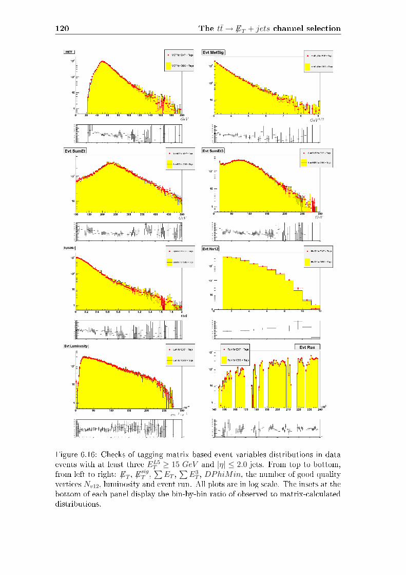
120 The tt→ 6ET + jets channel selection
Figure 6.16: Checks of tagging matrix based event variables distributions in dataevents with at least three EL5
T ≥ 15 GeV and |η| ≤ 2.0 jets. From top to bottom,from left to right: 6ET , 6E
sigT ,∑ET ,
∑E3
T , DPhiMin, the number of good qualityvertices Nv12, luminosity and event run. All plots are in log scale. The insets at thebottom of each panel display the bin-by-bin ratio of observed to matrix-calculateddistributions.

6.9 Positive b-tagging rate parameterization 121
Figure 6.17: Tagging matrix check after prerequisites application and before anykinematical selection. Observed and predicted positive b-tags as a function of thejet multiplicity. The expected contribution coming from tt events is also shown,see text for details.
The consequence of this is that we need to remove the tt contribution in each jetbin in order to have a background-only determination of the number of expectedb-tags. To do so, we iteratively correct the number of expected b-tags for each jetmultiplicity as follows [22]:
N ′exp = N fix
exp
Nevt −N ttevt
Nevt
= N fixexp
Nevt − Nobs−Nexp
εavetag
Nevt
(6.14)
where, for a chosen jet multiplicity:
• N fixexp is the number of expected tags for that jet multiplicity coming from the
tag rate parameterization before any correction; this number is �xed duringthe iterative procedure.
• Nevt is the number of events in the pre-tagging data sample of that jet mul-tiplicity used to determine N fix
exp through the tag matrix prediction;
• εavetag is the average tagging e�ciency, de�ned as the Monte Carlo ratio betweenthe number of positive b-tagged jets and the number of events in the pre-tagsample in the chosen jet multiplicity;
• N ttevt is the tt contamination in the pre-tagging sample of the chosen jet mul-
tiplicity, estimated as Nobs−Nexp
εavetag
.
The iterative procedure stops when the di�erence |N ′exp −Nexp| ≤ 1%.
The results of this approach are shown in Fig. 6.17, where we assumed a ttproduction cross section σtt = 6.7 pb for the Monte Carlo. The red error bands inthe plot are statistical only and come from the tag matrix application: we recallthat for each matrix bin, the tag rate is calculated as N+
bin/Ntaggablebin with N+
bin

122 The tt→ 6ET + jets channel selection
Figure 6.18: Tagging matrix check after prerequisites application and before anykinematical selection. Observed and predicted positive b-tags as a function of Neu-ral Network output. Left plot shows the predictions for data events with at leastthree tight jets, right plot for at least four tight jets. The expected contributioncoming from tt events is also shown, see text for details.
being the number of positive tagged jets and N taggablebin the number of taggable jets
in that matrix bin in the 3-jets sample used for matrix parameterization. We thuspropagate the error associated with this ratio to the expected number of tags.
Once we take into account the tt signal contamination in the sample and itscontribution to the number of observed b-tags, the agreement between the numberof observed and predicted b-tags is good in all the jet multiplicity bins, beingexactly the same by de�nition for 3-jet events, on which the matrix is calculated.
b-tagging rate extrapolation and Neural Network
An additional check we want to perform is related to the behaviour of the matrixpredictions with respect to the output of the Neural Network we will use later forour kinematical selection; we want to verify that the prediction of the backgroundworks well over all the spectrum of the output of the neural network. Fig. 6.18shows the output of the Neural Network and the corresponding background pre-diction from the tag matrix and the expected contribution from tt signal bothfor events with at least three tight jets and at least four tight jets. Matrix pre-dicted tags for bins with a considerable amount of signal contamination have beencorrected according to the iterative procedure described in Sec. 6.9.3.
Results are quite good over all the neural network spectrum, altough somediscrepancies arise mainly in the low output region. In the high neural networkoutput region we can see that the tagging matrix predictions are not su�cient tojustify the number of observed tags, while the agreement is good if we add theamount of tags coming from the expected tt signal contribution. This is both acon�rmation of the e�ectiveness of the method we used to estimate the backgroundand an additional check of the correct behaviour of the neural network we trained.
Fig. 6.19 shows the same kind of plot for 3, 4 and 5 tight jet events. As expected,agreement is very good in the 3 jets sample and this provides an additional checkof the fact that the matrix parameterization is not a�ected by the application ofthe neural network. Furthermore, since we don't expect a sizeable signal presence

6.9 Positive b-tagging rate parameterization 123
in the sample, the fact that the vast majority of 3 jet events has a neural networkoutput close to zero is again an indication of a well trained network. The behaviourof the matrix predictions in the 4 and 5 jets data samples is less accurate andmore a�ected by statistical �uctuations mainly due to the fact that bins are lowpopulated, but further highlights the desired features of the network, that classi�esas expected the signal events.
Figure 6.19: Tagging matrix check after prerequisites application and before anykinematical selection. Observed and predicted positive b-tags as a function ofNeural Network output. Upper left plot shows the predictions for data events withexactly three tight jets, upper right plot is in log scale. Bottom left plot showsthe predictions for data events with exactly four tight jets, bottom right plot fordata events with exactly �ve tight jets. The expected contribution coming from ttevents is also shown, see text for details.

124 The tt→ 6ET + jets channel selection
6.10 Event selection
In this section the optimization procedure we adopted to set the best values ofthe neural network output cut will be described.
As previously described, b-jet identi�cation provided by the secvtx algorithmconstitutes an e�ective handle to discriminate the tt production against backgroundprocesses. The �nal data sample to be used for a cross section measurement willthus be obtained by applying, in addition to the neural network selection, therequirement of at least one positive secvtx tagged jet.
The optimization procedure we seek is aimed at minimizing the statistical un-certainty on the cross section measurement, in order to optimize the measurementin terms of the expected number of b-tags over the background prediction. Theformer quantity is evaluated from inclusive Monte Carlo tt sample, the latter isderived from the b-tagging matrix application to data.
6.10.1 Optimization and Best Cut
After the clean up cuts described in Sec. 6.6, the analysis selection starts byasking for multijet data events with at least four jets with EL5
T ≥ 15 GeV and|η| ≤ 2.0: 3-jet data events are not considered in the optimization procedure sincethey are used for the b-tagging rates parameterization and thus are intrinsicallybiased.
The optimization procedure for the event selection de�nition is performed afterthe Njets ≥ 4 requirement and scans di�erent cuts on neural network output;among all possible cut con�gurations it chooses the one promising the minimumrelative statistical error on the cross section measurement.
The central value of the production cross section we want to measure is givenby:
σ(pp→ tt)×BR(tt→ 6ET + jets) =Nobs −Nexp
εkin · εavetag · L
(6.15)
where Nobs and Nexp are the number of observed and matrix-predicted tagged jetsin the selected sample, respectively; εkin is the trigger, prerequisites and neural net-work selection e�ciency measured on inclusive Monte Carlo tt events; εave
tag , de�nedas the ratio of the number of positive tagged jets to the number of pre-taggingevents in the inclusive tt Monte Carlo sample, gives the average number of b-tagsper tt event. Finally, L is the luminosity of the dataset used.
Using in input to Equation 6.15 the measured kinematical e�ciency, the aver-age number of b-tags per tt event, the actual integrated luminosity and the numberof b-tagged jet expected from the tag rate parameterization in the selected sample,we can estimate the expected cross section value and its relative statistical uncer-tainty for each neural network cut. The only missing piece is Nobs. We cannotuse the actual number of observed b-tags in the selected data, since it would biasour conclusion given its possible statistical �uctuations. For this reason, in orderto obtain an a priori determination of the best cut, we substitute Nobs with theexpression Nexp +NMC , where Nexp and NMC are the number of expected b-taggedjets from the tagging rate application and from inclusive tt Monte Carlo samples

6.10 Event selection 125
Figure 6.20: From top to bottom, from left to right: MCevt and Dataevt, NMC andNexp, εkin and εave
tag , S/B ratio and signal statistical signi�cance S/√S +B as a
function of the cut on the Neural Network output. MCevt and NMC have not beenrescaled to their expectation value in 1.9 fb−1. S/B and εave
tag plots show e�ectsdue to low statistics for cuts on neural network output in the region close to 1.
after the application of the given neural network cut, respectively. Using these val-ues, the statistical uncertainty a�ecting the measurement can be computed before

126 The tt→ 6ET + jets channel selection
Figure 6.21: Expected relative statistical error on the cross section measurementσxsec/xsec versus neural network cut. Best cut is set as NNout ≥ 0.92.
looking at the �post-tagging� data sample, allowing in this way to choose the cutminimizing the relative error on the cross section measurement.
For each neural network output cut the following quantities are calculated:
• MCevt, and Dataevt: number of inclusive Monte Carlo tt and data events inthe selected sample, before any b-jet identi�cation requirement.
• NMC and Nexp: number of positive tags expected from Monte Carlo inclusiveevents and from tagging rate parameterization after the kinematical selectionde�ned by the cut on the neural network output. Since we want to derivea �blind� minimization procedure, we don't want to look at the post-taggingsample, meaning we won't use any information on the number of observedb-tags Nobs in the sample obtained after the neural network cut. Since Nobs
is necessary for our iterative correction procedure, we will then rely on theuncorrected matrix predictions only.
• εkin and εavetag are derived from the application of the cut to the Monte Carlo
sample.
• the signal statistical signi�cance obtained as S/√S +B: ratio of the number
of tags expected for tt events and the square root of the number of tagsexpected from background processes plus the number of tags expected fromsignal.
• σxsec/xsec: relative error on the cross section measurement.
Results are reported in Fig. 6.20, while Fig. 6.21 shows the cross section uncertaintyversus the neural network output cut, calculated using only the statistical errorsof the involved quantities.
The �nal result of this procedure sets as the best event selection cut NNout ≥0.92, promising a relative statistical cross section uncertainty of 8.6% and a S/B

6.10 Event selection 127
ratio in terms of positive tags due to signal versus tags coming from backgroundprocesses of 2.18. The pre-tagging combined kinematical e�ciency of trigger, eventclean-up, and neural network cut on tt inclusive events is measured to be εkin =4.907 ± 0.001%, where the uncertainty is statistical only. The average number oftags per tt event under these selections is found to be εave
tag = 0.8188± 0.0008, andis determined by dividing the number of b-tagged jets in the kinetically selectedsample (Ntag = 187, 201) by the number of inclusive tt events surviving the selection(Nevt = 228, 614). The εkin and εave
tag values will be used for the cross sectionmeasurement as it will be described in Chapter 7.
Previous kinematical selection and new trigger e�ect
MC inc. tt ttopel εcut(%) ttop75 ot εcut(%) ttop75 nt εcut(%)Tot. evts 4719385 − 4719385 −Good Run 1021924 − 3979960 − 3979960 −Trigger 2579315 64.81 2311270 58.07Vertex Req. 2466709 95.63 2213324 95.76Lepton Veto 558528 − 2196636 89.05 1982264 89.56NJet ≥ 4 549138 98,32 2156643 98.18 1958949 98.826ET
sig ≥ 4 GeV 1/2 78145 14.23 309425 14.35 238426 12.17DPhiMin ≥ 0.4 49848 63.79 197264 63.75 145197 60.90Tot. E�. 4.88 4.96 3.65
Table 6.5: E�ect of the introduction of the new L2 TOP_MULTI_JET triggeron inclusive tt Monte Carlo events. The column for ttopel shows results takenfrom [3]; the one for ttop75 ot shows the results obtained on ttop75, the MonteCarlo dataset used in our neural network analysis, after a full simulation of the oldtrigger. Column for ttop75 nt show the results of the selection on ttop75 with afull simulation of the new trigger path. For each cut, the e�ciency with respectto the previous selection is provided. Last line shows the overall e�ciency of theselection. The expected loss in the e�ciency of the selection on inclusive tt signaldue to the introduction of the new trigger is ∼ 26.4%.
The kinematical selection studied in [3] for the cross section measurement inthe tt→ 6ET +jets channel with the 311 pb−1 data sample was optimized for the oldTOP_MULTI_JET trigger path and reached a kinematical e�ciency on inclusivett events of εkin = 4.878± 0.021%.
Tab. 6.5 shows the e�ect caused on this kinematical selection by the intro-duction of the higher energy treshold in the new Level 2 requirements of theTOP_MULTI_JET trigger, starting from Run 194328 (see 6.2 for details). Re-sults in the table are obtained with a Good Run List older than the one used inour analysis.
First two columns, referring to the dataset ttopel, show results of the selectionon inclusive tt Monte Carlo events, taken from the published article [3]. For com-parison, the results of the old selection on the inclusive Monte Carlo dataset used in

128 The tt→ 6ET + jets channel selection
this analysis, ttop75, treated with a full simulation of the old TOP_MULTI_JETtrigger path are reported in the two central columns (�ttop75 ot�). Relative e�-ciencies of the di�erent selections agree very well, and thus give us the possibility ofestimating the e�ect of the new trigger introduction by simulating its requirementson ttop75. The e�ects of the new trigger and the kinematical selection are shownin the last two columns of Tab. 6.5 under the label �ttop75 nt�. Relative e�cienciesof the analysis kinematical cuts are almost left unchanged by the introduction ofthe new trigger, but we notice an overall reduction of the kinematical e�ciencyon the sample with the new trigger simulation from 4.96± 0.01% to 3.65± 0.01%,causing an expected tt signal loss around the 26.4% with respect to the previoustrigger.
It is interesting to note that the neural network selection described in this workachieves an e�ciency εkin = 4.907 ± 0.001% on tt inclusive events taken with thenew trigger path, comparable with the one obtained in [3] for the old trigger. Inconclusion, with the introduction of the neural network selection we were thenable to mitigate the e�ect of the new trigger on the signal acceptance of the oldkinematical selection in this decay channel.
Event selection acceptances
The impact of the trigger, prerequisites and optimized neural network selectionon exclusive e + jets, µ + jets, τ + jets, all-hadronic and di-lepton tt MonteCarlo events is shown in Tab. 6.6. We note that, as expected, the di-lepton decaychannel is highly suppressed by our choice of TOP_MULTI_JET trigger, that isnot designed for this kind of analysis. Moreover, the all-hadronic tt decay channel ishighly suppressed by the requirement of large missing ET signi�cance 6ET/
√ΣET ≥
3 GeV 1/2: as we already pointed out, this analysis prerequisite rejects those eventswhose missing ET is due mainly to residual energy mis-measurement e�ects, suchas all-hadronic events, while it focuses on events containing physics-induced 6ET .
Considering the leptonic decay channels, we note that the selection we describedallows tt isolation by requiring the presence of large 6Esig
T in the event, thus searchingfor high-PT neutrino signature produced in the leptonic decay of theW boson. Thissignature is produced in a similar way for all the top pair e + jets, µ + jets andτ + jets decay channels.
Even if we didn't use any lepton identi�cation procedure and despite the well-identi�ed high-PT lepton veto imposed for e and µ, the �nal acceptance providedby the kinematical selection is comparable for all the lepton+jets decays. Thee�ciencies calculated with respect to the number of events for each decay mode ofall selection requirements are found to be 9.44± 0.03%, 7.38± 0.03% and 12.66±0.04% for e+ jets, µ+ jets and τ + jets channels respectively.
This is due to the fact that the trigger requirement has a large impact on µ+jetstt decays with respect to the other leptonic ones (the muons does not make anyjet), while the tight lepton veto prerequisite decreases the selection e�ciency forboth e and µ plus jets events. Additionally, the relative e�ciency for the 6Esig
T
selection with respect to the Njet requirement is more or less the same for τ andelectron plus jets events, but it is higher for muon: we correct the 6ET for muontransverse momentum but we do not include the muon PT in the calculation of the

6.10 Event selection 129
N evt tt e+ jets εcut(%) µ+ jets εcut(%) τ + jets εcut(%)Branching Ratio 689,083 − 688,787 − 689,743 −Good Run 680,317 − 679,962 − 680,758 −Trigger 411,734 60.52 201,436 29.62 315,536 46.35Vertex Req. 393,562 95,59 193,513 96.07 302,867 95.98Lepton Veto 220,834 56.11 128,906 66.61 285,637 94.31NJet ≥ 4 215,022 97.37 124,367 96.48 280,032 98.046ET
sig ≥ 3 GeV 1/2 117,360 54.58 82,472 66.31 160,683 57.38NNout ≥ 0.92 65,072 55.45 50,819 61.62 87,352 54.36Tot. E� wrt BR 9.44 7.38 12.66
N evt tt all-hadronic εcut(%) di-lepton εcut(%)Branching Ratio 2,154,096 − 221,659 −Good Run 2,126,366 − 218,737 −Trigger 1,744,325 82.03 18,555 8.48Vertex Req. 1,673,326 95.93 17,172 92.55Lepton Veto 1,672,094 99.93 7,853 45.73NJet ≥ 4 1,662,229 99.41 7,089 90.276ET
sig ≥ 3 GeV 1/2 74,833 4.50 4,890 68.98NNout ≥ 0.92 10,432 13.94 2,851 58.30Tot. E� wrt BR 0.48 1.29
Table 6.6: E�ect of the trigger, prerequisites and neural network selection cutsfor e/µ/τ + jets (top) and all-hadronic and di-lepton (bottom) exclusive tt MonteCarlo events. For each cut, the e�ciency with respect to the previous selection isprovided for each tt decay channel. Last line shows the overall e�ciency of theselection with respect to the branching ratio of the channel.
event∑ET . This increases the possibility for a µ + jets event to pass this cut,
given that√∑
ET is the denominator of the missing ET signi�cance. The samee�ect happens for the neural network selection cut, that is sensitive to the event∑ET and missing ET signi�cance since it uses these two variables as inputs: the
neural network cut shows a higher e�ciency on µ+ jets tt decays.Overall, the described event selection provides comparable e�ciencies in the
pre-tagging sample and thus selects comparable tt signal contributions from eachlepton+jets decay mode. Rescaling the number of Monte Carlo events surviving theselection according to the 1.9 fb−1 data luminosity, we expect about 178/139/239events from e/µ/τ + jets decays, respectively.
Background prediction systematic uncertainty
The optimized neural network cut de�nition found in previous sections allowsus to de�ne control data samples in which to further check the b-tagging rateparameterization for the background. In fact, once the selection is de�ned, wecan reverse its cut to construct control data samples close to the signal region butdepleted as much as possible of signal contribution, where to compare the number

130 The tt→ 6ET + jets channel selection
N jet 3 4 5 6 7 8
Obs + tags 2230 4977 3361 1329 405 76Exp + tags 2231.18 4974.27 3231.98 1259.23 359.62 80.26error ±51.34 ±130.05 ±93.99 ±40.52 ±14.22 ±4.96Exp/Obs ratio ≈ 1 ≈ 1 0.96 0.95 0.89 1.06
Table 6.7: Tagging matrix check in the data sample with NNout <= 0.9. For eachjet multiplicity bin, the number of observed and predicted positive b-tags is shown.Uncertainties are statistical only.
Exp + tags, N Jets: 3 4 5 6 7 8
Complete mtx 2238 5049.75 3336.98 1335.07 389 90.77error ±51.53 ±134.08 ±99.18 ±43.66 ±15.52 ±5.49Even mtx 2261.82 5050.97 3369.02 1342.38 392.39 91.09error ±84.09 ±208.51 ±156.68 ±72.64 ±24.09 ±7.87Odd mtx 2184.92 4851.31 3153.2 1258.63 357.03 80.67error ±86.67 ±210.09 ±158.72 ±69.22 ±24.76 ±8.69Even−OddComplete
ratio (%) 3.44 3.95 6.47 6.27 9.09 11.48
Table 6.8: Even-odd tagging matrix check in the complete data sample after pre-requisites. For each jet multiplicity bin, the number of predicted positive b-tagswith the complete, even and odd matrix is shown. Uncertainties are statisticalonly.
of observed positive tags to the number of predicted tags derived from the taggingrate parameterization applied to data. This will allow us to verify the predictionsof the matrix and to account for possible deviations from the desired behaviourderiving a systematic uncertainty on the background prediction.
The �rst sample we want to analyze is made of events with NNout <= 0.9.The performances of the tagging matrix as a function of the jet multiplicity areshown in Tab. 6.7. The agreement is quite good and any discrepancy can be limitedat the level of few percent.
Additionally, we can try to give an estimate of how our background predictionsare a�ected by statistical �uctuations in the sample we used to construct the matrixparameterization. To do so, we split our 3-jets data sample after prerequisites ineven and odd events and use this two orthogonal samples to build two tag matrixeswith the same characteristics of the one we used in the analysis.
The comparison of the tag rates obtained with these two samples and the onesused in the analysis is shown in Fig. 6.22. We now use the matrixes to derivethe number of expected positive b-tags for each jet multiplicity in the data sampleobtained after prerequisites application, and account any discrepancy among thetwo and the complete matrix as a systematic error on our background prediction.Tab. 6.8 shows the results of this additional check.
From the studies performed, a systematic uncertainty on the background pre-diction can be derived.

6.10 Event selection 131
Figure 6.22: Tag Rates for the variables jet ET , jet Ntrk and 6ETprj used in the
matrix parameterization are compared for the matrix built using all 3-jets dataand for the odd and even matrixes.
Considering the obs/exp b-tag ratio as a function of the jet multiplicity , theoverall discrepancy between observed and matrix predicted number of b-tags dueto intrinsic limits of the matrix and to the dependance from the sample in whichthe matrix has been built can be quoted conservatively at 15%. This value willbe assumed as the systematics uncertainty to be associated to our backgroundprediction, and will be used in Chapter 7 for the cross section measurement.

132 The tt→ 6ET + jets channel selection

Bibliography
[1] F. Abe et al., The mu tau and e tau Decays of Top Quark Pairs Produced in panti-p Collisions at
√s = 1.8 TeV , Phys. Rev. Lett. 79, 3585 (1997).
[2] G. Cortiana et al.,Measurement of the tt production cross section in the τ+jetschannel with SecVtX tags using 311pb−1 of pp data, CDF Internal Note 7689.
[3] A. Abulencia et al. [CDF Collaboration], Measurement of the tt productioncross section in pp collisions at
√s = 1.96 TeV using 6ET + jets events with
secondary vertex b-tagging, Phys. Rev. Lett. 96, 202002 (2006).
[4] T. Sjostrand et al., High-energy-physics event generation with PYTHIA 6.1,Comput. Phys. Commun. 135 238 (2001), [arXiv:hep-ph/0010017].
[5] G. Corcella et al., HERWIG 6: An event generator for hadron emission reac-tions with interfering gluons (including supersymmetric processes), JHEP 0101
010 (2001), [arXiv:hep-ph/0011363].
[6] R. Brun et al., Geant: Simulation Program For Particle Physics Experiments.User Guide And Reference Manual, CERN-DD-78-2-REV.
[7] S. Carron et al., Parametric Model for the Charge Deposition of the CDF RunIISilicon Detectors, CDF Internal Note 7598.
[8] W. Riegler et al., COT detector physics simulations, CDF Internal Note 5050.
[9] S.Y. Jun et al., GFLASH Tuning in the CDF Calorimeter for the 2003 WinterRelease, CDF Internal Note 7060.
[10] TRIGSIM++ Web Page:http://www-cdf.fnal.gov/internal/upgrades/daq_trig/twg/trgsim/trgsim.html.
[11] D. Tsybychev et al., A study of missing ET in Run II minimum bias data,CDF Internal Note 6112.
[12] G. Cortiana et al., t tbar -> tau + jets nt5 analysis update, CDF Internal Note7553.
[13] S. Grinstein et al., Electron-Method SecVtx Scale Factor for Winter 2007,CDF Internal Note 8625.
[14] F. Garberson et al., SecVtx B-Tag E�ciency Measurement Using Muon Trans-verse Momentum for 1/fb Analyses CDF Internal Note 8434.

134 BIBLIOGRAPHY
[15] S. Grinstein and D. Sherman, SecVtx Scale Factors and Mistag Matrices forthe 2007 Summer Conferences, CDF Internal Note 8910.
[16] F. Garberson et al., Combination of the SECVTX b-Tagging Scale Factors for1 fb-1 Analyses, CDF Internal Note 8435.
[17] V.D. Barger, R.N. Phillips, Collider Physics, Addison-Wesley (1987).
[18] T. Aaltonen et al. [The CDF Collaboration], Measurement of the Top PairProduction Cross Section in the Lepton+Jets Decay Channel, CDF Public Note8795.
[19] T. Aaltonen et al. [The CDF Collaboration], Measurement of the ttbar CrossSection and Top Quark Mass in the All Hadronic Channel, Phys. Rev. D 76,072009 (2007).
[20] Data Quality Web Page:http://www-cdf.fnal.gov/internal/dqm/goodrun/v17/goodv17.html.
[21] K. Copic and M. Tecchio, Event vertex studies for dilepton events, CDF In-ternal Note 6933.
[22] A. Castro et al., Top Production Cross Section in the all-hadronic channel,CDF Internal Note 3464.
[23] G. Cortiana et al., Background studies for the tt → τ + jets search, CDFInternal Note 7292.

Chapter 7
Cross section measurement and
systematic uncertainties
In this Chapter we will �nalize our tt → 6ET + jets cross section measure-ment. After describing the �nal data sample obtained with our neural networkselection, we will analyze and discuss the sources of systematic uncertainties and�nally we will determine the cross section measurement by means of a likelihoodmaximization.
7.1 The �nal sample
The optimized neural network selection described in previous chapter allowsto isolate a tagged data sample in which the tt → 6ET + jets signal is estimatedto contribute with a signal to background ratio of at least S/B ∼ 2 after the re-quirement of selecting events containing at least one positive secvtx tagged jet.Indeed the tagging probability for a b-jet produced by top quark decay is expectedto be higher than the probability to identify b-quark jets yielded by backgroundprocesses. Additionally, the selection is expected to provide a statistical uncer-tainty of 8.6% on the cross section measurement. Moreover, we will see at the endof this section that after the correction of the expected background for the pres-ence of signal in the pre-tagging sample used for b-tagging rate parameterizationapplication, the S/B ratio will increase to ∼ 4.5, since almost 50% of the expectedbackground b-tags will be found to be due to tt contamination.
Fig. 7.1 displays the sample composition after the cut on the neural network:the predicted amount of background b-tags after the selection is shown togetherwith the expected inclusive tt contribution; the observed positive tags in the dataare shown by dots. After selection we are left with a sample containing 1415 events,and 627 positive b-tags.
As already discussed, since the data events selected before the tagging require-ment are expected to contain a non-negligible tt component, the tagging rate pa-rameterization procedure overestimates the background. We correct for this e�ecteach jet multiplicity bin of Fig. 7.1 using the iterative procedure discussed in pre-vious chapter.
A good agreement between observed and predicted background tags is noted

136 Cross section measurement and systematic uncertainties
Figure 7.1: Number of tagged jets versus jet multiplicity. Data (points), iterativelycorrected background (yellow histogram) and tt expectation (blue histogram) forσtt = 6.7 pb are shown after neural network selection.
in the 3-jet bin, where the tagging matrix is computed before the kinematicalselection, while on the contrary for 4 to 8 jet bins the addition of Monte Carloinclusive contribution is required in order to explain the data behavior. However,the 4-jets bin shows a noticeable mismatch between the number of observed andpredicted b-tags: this e�ect is still under investigation.
Now that we estimated the tt component in the selected sample and the overallbackground to the signal signature by means of the tagging rate parameteriza-tion applied to data, we can �nally provide the top pairs production cross sectionmeasurement in the selected data sample.
We have all the ingredients to proceed directly for a measurement, we areonly missing the systematic uncertainties determination. The measurement wewill describe uses the excess of b-tagged jets over the background prediction toestimate the top pairs production cross section. In order to properly account foreach systematic source a�ecting the measurement, a likelihood function will beused to determine the cross section value.
The cross section measurement will be obtained by maximizing logL, wherethe likelihood function is de�ned as follows:
L = e− (L−L)2
2σ2L · e
− (εkin−εkin)2
2σ2εkin · e
−(εave
tag−εavetag )2
2σ2εavetag · e
− (Nexp−Nexp)2
2σ2Nexp · (7.1)
·(σtt · εkin · εave
tag · L+Nexp)Nobs
Nobs!· e−(σtt·εkin·εave
tag ·L+Nexp)
where L is the integrated luminosity of the data sample we used, εkin is the com-bined trigger, prerequisites and neural network selection e�ciency on inclusiveMonte Carlo tt events, and εave
tag is the average number of b-tags per tt event. Nexp
is the number of background b-tags returned by the tagging matrix application tothe selected data sample; Nobs is the number of observed b tags in the data.

7.1 The �nal sample 137
Figure 7.2: Results of background correction, see text for details.
The cross section central value is then given by the likelihood maximization as:
σtt =Nobs −Nexp
εkin · εavetag · L
(7.2)
In the following, we review the input values we need to perform the likelihoodmaximization.
In previous Chapter we determined the overall kinematical e�ciency and theaverage number of b-tagged jets per tt event to be εkin = 4.907±0.001% and εave
tag =0.8188±0.0008 respectively. Using the tagging rate parameterization applied to the1415 events passing the selection, the background amount in terms of b-tagged jetsis calculated to be 237.64± 15.28(stat)± 35.64(syst) = 237.64± 38.77, where the�rst uncertainty is statistical only, while the latter is systematic and is calculated bycomparing observed to matrix-predicted b-tags in data control samples and quotinga 15% systematic uncertainty. This value needs to be corrected for the signalpresence in the pre-tagging sample, as seen in the previous chapter: the applicationof our iterative correction procedure yelds a top-free background determination ofN corr
exp = 137.5. The uncertainty on the background correction depends both onthe uncertainty on Nexp and the uncertainty on εave
tag . In order to evaluate bothcontributions we follow the tecnique adopted in [1]: we generate 1, 000, 000 randomsamples of Nexp events smeared with its ±15.28 statistical uncertainty and applythe iterative correction using εave
tag smeared with its statistical uncertainty. Theresulting Nexp distribution is shown in Fig. 7.2 and gives N corr
exp = 137.5± 11.2, sothe relative statistical uncertainty on the expected background becomes 8.1%.
On the other hand, the number of observed b-tagged jets in the data sampleselected with the neural network selection is found to be 627.
Finally, the integrated luminosity of the considered data sample is L = 1906.8±110.6 pb−1.
For a proper determination of the cross section, we need to assign to each ofthe input values its corresponding uncertainty, accounting for both the statisticaland systematic e�ects.
In the following the sources of systematic uncertainty will be described andquanti�ed.

138 Cross section measurement and systematic uncertainties
N evt PYTHIA HERWIG
Tot. Events 4,719,385 − 979,066 −Good Run 4,658,603 − 975,615 −L2 Trigger 2,786,636 59.82 % 608,639 62.39 %L3 Trigger 2,719,975 97.61 % 595,200 97.79 %Good Vertex 2,607,087 95.85 % 569,944 95.76 %Nlep = 0 2,333,998 89.53 % 505,885 88.76 %Njet ≥ 3 2,333,351 99.97 % 505,714 99.97 %6ET/
√ΣET ≥ 3 GeV 1/2 464,067 19.89 % 109,140 21.58 %
Njet ≥ 4 452,009 97.40 % 106,141 97.25 %
Table 7.1: E�ect of the trigger and prerequisites selection on PYTHIA and HER-WIG inclusive tt generated events. Last requirement before neural network appli-cation is is Njet(E
L5T ≥ 15, |η| ≤ 2.0) ≥ 4.
7.2 Systematics
7.2.1 Background prediction systematic
The systematic uncertainty on the background prediction is calculated, as al-ready explained in previous Chapter, by comparing the number of b-tags yeldedby the tagging matrix application to the actual number of positive secvtx tagsin a control sample depleted of signal contamination (we chose the one withNNout ≤ 0.9), obtained from the TOP_MULTI_JET triggered dataset; addition-ally, another source of systematic uncertainties has been considered, depending onthe statistical �uctuations in the sample used for the tagging matrix parameteri-zation. As a result of these checks a 15% systematic uncertainty to the number ofbackground b-tags returned by the tagging matrix application to data is assigned.
7.2.2 Luminosity systematic
The integrated luminosity calculation is based on the instantaneous luminositymeasurement provided by the CLC detector described in Sec. 3.5. Two compo-nents of uncertainty play a role in the luminosity measurement determination: theacceptance and operation of the luminosity monitor (the CLC detector) and thetheoretical uncertainty of the total inelastic pp cross section (60.7± 2.4 mb). Theuncertainties on these quantities are 4.2% and 4.0% respectively, giving a totaluncertainty of 5.8% on the integrated luminosity calculated for any given CDFdataset [2].
7.2.3 Monte Carlo generator dependent systematics
The base Monte Carlo sample adopted for this work consists of almost 4 millionsinclusive tt events (exactly 3, 979, 960 after the Good Run requirement) generatedusing PYTHIA with Mtop = 175 GeV/c2, and with corresponding integrated lumi-nosity of 594 fb−1 assuming σtt = 6.7 pb.

7.2 Systematics 139
Figure 7.3: Top: kinematical e�ciency of trigger, prerequisites and neural net-work selection versus cut applied on neural network output for both PYTHIAMonte Carlo sample (ttop75) and HERWIG sample (htop75) generated at Mtop =175 GeV/c2. Bottom: Monte Carlo generator dependent systematic versus cut onneural network output. The error peak for neural network output cuts close to 1is due to low statistics e�ects.
The neural network selection optimization was derived using these PYTHIAinclusive tt Monte Carlo events. In order to evaluate the generator dependence ofthe kinematical e�ciency computed for signal events we used a sample of almost1 million (exactly 975, 615 after the Good Run requirement) tt events generatedwith HERWIG, corresponding to an integrated luminosity of 145.6 fb−1.
All these samples are processed through the CDF detector and trigger simula-tion, as described in Sec. 6.1.
Tab. 7.1 shows the e�ect of each cut of trigger and prerequisites selection,before neural network application, for inclusive tt events generated with PYTHIAand HERWIG. The e�ciency of each cut with respect to the previous one is alsoreported.
The overall systematic uncertainty to be assigned to generator e�ects can thenbe computed for each neural network output cut as:
systgen(cut) =∆ε(cut)
ε(cut)=εHERWIG(cut)− εPY THIA(cut)
εPY THIA(cut)(7.3)
where εPY THIA(cut) and εHERWIG(cut) are the kinematical e�ciency for thechosen cut on tt inclusive Monte Carlo events generated with PYTHIA and HER-WIG, respectively. Fig. 7.3 shows the results of this calculation in the 0.8 − 1.0neural network output cut range.
For the optimized cut we chose in previous chapter NNout ≥ 0.92 the corre-sponding systematic uncertainty to be assigned to generator dependence e�ects issystgen = 10.84%.

140 Cross section measurement and systematic uncertainties
Figure 7.4: PDF dependent systematic, obtained with Monte Carlo reweightingtecnique, versus cut on neural network output. The error increases for neuralnetwork output cuts close to 1 because of low statistics e�ects.
7.2.4 PDF-related systematics
The parton distribution functions (PDFs) chosen for the standard CDF MonteCarlo generation correspond to the CTEQ parameterization outlined in [3]. Thereare uncertainties associated with this parameterization, since the usage of di�erentparameterizations of the PDFs could slightly change the kinematics and thus theacceptance for signal events.
In order to account for these e�ects, we used a standard Monte Carlo reweight-ing tecnique. Instead of generating new samples for each di�erent PDF, we re-weighted the events already generated with PYTHIA according to di�erent PDFeigenvectors. The weight for each event is calculated as the ratio of the new PDFswith respect to the standard one. We then sum the weights in order to determinethe e�ect on the total kinematic e�ciency [4].
The results of the calculation for neural network output cuts in the range 0.8−1.0 are shown in Fig. 7.4. For the optimized cut we chose in previous chapterNNout ≥ 0.92, as a result of this approach we set a systPDF = 1.64% systematicuncertainty associated with our choice of PDFs.
7.2.5 ISR/FSR-related systematics
In general it is very di�cult for Monte Carlo generators to model accuratelyinitial and �nal state radiation processes. If more or less extra radiation is presentin the event with respect to the default values set in the base Monte Carlo sample,the event kinematics could change a�ecting the kinematic e�ciency determination.Indeed the presence of less or more radiation associated to the tt production canalter the acceptance of the Njet and 6ET/
√ΣET requirements.
We evaluated this e�ect using di�erent inclusive Monte Carlo tt samples gen-erated with di�erent tunings for initial (ISR) and �nal state (FSR) radiation:less/more ISR, and less/more FSR.
The impact of trigger and prerequisites selection for di�erent ISR/FSR radia-tion settings is presented in Tab. 7.2.

7.2 Systematics 141
N evt MCincl less ISR more ISR
Tot. Events 1,180,947 − 1,172,571 −Good Run 1,165,597 − 1,157,221 −L2 Trigger 701,208 60.16 % 714,682 61.76 %L3 Trigger 684,004 97.55 % 698,426 97.73 %Good Vertex 656,016 95.91 % 669,708 95.89 %Nlep = 0 588,301 89.68 % 598,031 89.30 %Njet ≥ 3 588,128 99.97 % 597,845 99.97 %6ET/
√ΣET ≥ 3 GeV 1/2 118,009 20.07 % 122,629 20.51 %
Njet ≥ 4 114,694 97.19 % 119,349 97.33 %
less FSR more FSR
Tot. Events 1,150,650 − 1,142,486 −Good Run 1,135,300 − 1,127,136 −L2 Trigger 693,212 61.06 % 684,307 60.71 %L3 Trigger 676,968 97.66 % 668,192 97.65 %Good Vertex 648,582 95.81 % 640,481 95.85 %Nlep = 0 579,746 89.39 % 573,900 89.60 %Njet ≥ 3 579,571 99.97 % 573,729 99.97 %6ET/
√ΣET ≥ 3 GeV 1/2 118,308 20.41 % 115,643 20.16 %
Njet ≥ 4 115,022 97.22 % 112,548 97.32 %
Table 7.2: E�ect of ISR/FSR radiation variation on trigger and prerequisites se-lection, before neural network application.
Here and in the next sections, we will calculate systematic e�ects for each cuton neural network output with the following approach: taking as an example thesystematic uncertainty to be related to initial state radiation e�ect we will computeit as:
systISR(cut) =|ε+ISR(cut)− ε−ISR(cut)|
2εPY THIA(cut)
when our nominal value for the kinematical e�ciency εPY THIA(cut) is in betweenthe values ε+ISR(cut) and ε−ISR(cut) we use for comparison; when it is not, we willuse half the maximum di�erence:
systISR(cut) =max (|ε+ISR(cut)− εPY THIA(cut)|, |εPY THIA(cut)ε−ISR(cut)|)
2εPY THIA(cut)(7.4)
The same will hold on the other hand for �nal state radiation e�ect, wich wewill compute for each cut as:
systFSR(cut) =|ε+FSR(cut)− ε−FSR(cut)|
2εPY THIA(cut)
or
systFSR(cut) =max (|ε+FSR(cut)− εPY THIA(cut)|, |εPY THIA(cut)− ε−FSR(cut)|)
2εPY THIA(cut)

142 Cross section measurement and systematic uncertainties
Figure 7.5: Top: kinematical e�ciency of trigger, prerequisites and neural networkselection versus cut applied on neural network output for PYTHIA Monte Carlosample (ttop75) and samples generated with more and less initial state radiation.Bottom: Initial state radiation systematic uncertainty versus cut on neural networkoutput. The behaviour of the error function for neural network output cuts in theregion close to 1 is due to low statistics e�ects.
according to the criteria described above.
Fig. 7.5 and Fig. 7.6 show the results of this calculation in the 0.8− 1.0 neuralnetwork output cut range for both the ISR and FSR contributions respectively.
For the optimized cut NNout ≥ 0.92, we can estimate a systematics to beassigned to initial state radiation e�ects of systISR = 2.86%, and a systematic for�nal state radiation e�ects of systFSR = 1.71%. Summing in quadrature the twoe�ects we can estimate a total systematic uncertainty to be assigned to initial and�nal state radiation e�ects of systISR/FSR = 3.33%.
7.2.6 Systematics due to the jet energy response
In this section we discuss the systematic uncertainty related to the jet energyresponse. In Sec. 4.3.1 the total systematic uncertainty on the corrected jet ET
was found to vary in the range [3,10]%, where the extreme values are reached forhigh and low jet ET , respectively. Moreover, the uncertainty associated to thejet energy response was found to be largely independent of the level of correctionapplied but to be mostly arising from the jet description provided by the MonteCarlo simulation.
In order to account for the jet response systematic in the cross section mea-surement, we varied the corrected jet energies within ±1σ of their correspondingsystematic uncertainty. Therefore, signal trigger and prerequisites e�ciencies arerecalculated after these variations. The results are provided in Tab.7.3.
As described in previous section, we can assign a systematic uncertainty de-

7.2 Systematics 143
Figure 7.6: Top: kinematical e�ciency of trigger, prerequisites and neural networkselection versus cut applied on neural network output for PYTHIA Monte Carlosample (ttop75) and samples generated with more and less �nal state radiation.Bottom: Final state radiation systematic uncertainty versus cut on neural networkoutput. The behaviour of the error for neural network output cuts close to 1 is dueto low statistics e�ects.
N evt MCincl standard jet corrs +1σ jet systs −1σ jet systs
Total 4,719,385 4,719,385 4,719,385Prereq 2,333,998 2,333,998 2,333,998Njet ≥ 4 2,306,282 2,310,830 2,300,0286ET/
√ΣET ≥ 3 GeV 1/2 452,009 469,481 449,568
Table 7.3: E�ect of the jet energy correction within their uncertainty on the triggerand prerequisites selection on tt inclusive events, before neural network application.
pending on the cut we apply on the neural network output as follows:
systjetcorr(cut) =|εjetcorr,+1σ(cut)− εjetcorr,−1σ(cut)|
2εkin(cut)
when our nominal value for the kinematical e�ciency εkin(cut) is in between thevalues εjetcorr,+1σ(cut) and εjetcorr,−1σ(cut), while in the other case we will use halfthe maximum di�erence de�ned according to Eq. 7.4.
Fig. 7.7 show the results of this calculation in the 0.8 − 1.0 neural networkoutput cut range.
For the optimized cut NNout ≥ 0.92, we can estimate a systematic uncertaintyto be assigned to jet energy response of systjetcorr = 4.73%.

144 Cross section measurement and systematic uncertainties
Figure 7.7: Top: kinematical e�ciency of trigger, prerequisites and neural networkselection versus cut applied on neural network output for the Monte Carlo sam-ple (ttop75) with standard jet corrections and with jet energy corrections shiftedby ±σ of their systematic error. Bottom: Systematic uncertainty due to jet en-ergy repsonse versus cut applied on neural network output. In the neural networkoutput cut region close to 1 low statistics e�ects arise, causing the error to increase.
7.2.7 b-tagging scale factor systematics
As described in Sec. 6.4, the secvtx e�ciency scale factor we used in thisanalysis, to count the number of b-tags on Monte Carlo events is SF = 0.95 ±0.050. Since the average number of b-tags per tt event, εave
tag , enters directly in thecross section measurement we have to compute the systematics e�ect related to itsdetermination.
In particular, to account for the scale factor uncertainty we varied it from itscentral value of 0.95 within the ±1σ range and we determined the di�erence interms of average number of b-tags per event on the Monte Carlo sample withrespect to the standard value, taking into account that the secvtx scale factorhas the same central value for both b- and c-quarks, but for the latter has a doubleduncertainty: SFb = 0.95± 0.050, SFc = 0.95± 0.100.
For each cut on neural network output we can assign the following systematicuncertainty:
systεtag(cut) =|εtag,+1σ(cut)− εtag,−1σ(cut)|
2εavetag (cut)
(7.5)
The results are shown in Fig. 7.8. As expected, the systematic uncertainty dueto the scale factor application does not depend much on the choice of the cut onthe network output, since it only rescales the number of positive tags in a givensample.
For the cut NNout ≥ 0.92, we can estimate a systematic uncertainty to beassigned to b-tagging scale factor application of systεtag = 3.98%.

7.2 Systematics 145
Figure 7.8: Top: Average tagging e�ciency in the sample obtained after trigger,prerequisites and neural network selection versus cut applied on neural networkoutput for the Monte Carlo sample (ttop75) with standard b-tagging Scale Factorand with Scale Factor shifted by ±σ of its systematic error. Bottom: Systematicuncertainty due to b-tagging scale factor application versus cut applied on neuralnetwork output. The behaviour of the error function in the output region closeto 1 is due to low statistic e�ects.
7.2.8 Trigger systematics
Trigger systematics have already been studied and characterized for the oldTOP_MULTI_JET trigger (used up to Run 194328) [6] using the following tec-nique. A sample of collider data called �Single Tower-10� is used, triggered withthe following requirements
• at Level 1: at least one calorimetric tower with ET ≥ 10 GeV .
• at Level 2: a static prescaling factor of 1K.
• at Level 3: auto-accept.
with a corresponding integrated luminosity of 196± 12 pb−1. This dataset is thenused to extract the e�ciency of the TOP_MULTI_JET trigger on a data-drivenbasis, evaluating its e�ciency by applying its L2 requirements directly on �SingleTower-10� triggered data.
Then the systematic uncertainty a�ecting the trigger e�ciency measurement onMonte Carlo tt events is evaluated by comparing trigger turn-on curves for Tower-10 data and bb and bb+6 partons Monte Carlo samples. The trigger turn-on curvesare derived as functions of of the 4th jet L5-corrected ET in the event.
From a study of the mismatch of turn-on curves between Monte Carlo samplesand data, a trigger e�ciency systematic of a few percent (2.0%) is derived.
Since we didn't have enogh time to reproduce such a detailed study of thetrigger turn-on curves for the new TOP_MULTI_JET trigger, we will rely on this

146 Cross section measurement and systematic uncertainties
Source Method Uncertainty
εkin systematics
Generator dependence |εPY THIA−εHERWIG|εPY THIA
10.84 %
PDFs MC reweighting 1.64 %ISR/FSR samples comparison 3.33 %
Jet Energy Scale|εjetcorr,+1σ−εjetcorr,−1σ |
2εkin4.73 %
Trigger simulation turn-on curves 2.0 %
εtag systematics
SecVtX scale factor |εtag,+1σ−εtag,−1σ |2εtag
3.98 %
Tagging matrix systematicsData control samples Nobs/Nexp 15.0 %
Luminosity systematicsLuminosity measurement − 5.8 %
Table 7.4: Summary of the sources of systematic uncertainty. Trigger simulationsystematic uncertainty is based on a determination on the old TOP_MULTI_JETtrigger and is to be considered a preliminary result.
Variable Symbol Input Value Output Value
Integrated Luminosity (pb−1) L 1906.8± 110.6 1907.1± 111.7Observed Tags Nobs 627 −Expected Tags N corr
exp 137.5± 23.4 137.1± 23.3Kin. e�ciency (%) εkin 4.907± 0.613 4.889± 0.668Ave. b-tagging e�ciency εave
tag 0.8188± 0.0325 0.8187± 0.0327
Table 7.5: Input and output values of the likelihood maximization.
previous determination to give a preliminary cross section measurement in thischannel.
7.3 Cross section measurement
The summary of all the sources of systematic uncertainty to the cross sectionevaluation is listed in Tab. 7.4.
Now that we have evaluated all the sources of systematic uncertainty a�ectingthe kinematical selection e�ciency as well as the determination of the averagenumber of b-tags per tt event and the background prediction, we are ready to useall the ingredients described in 7.1 to perform the cross section measurement.
We remind that we will interpret the excess in the number of tags de�ned asNobs − N corr
exp as a sign of tt production and it will be used for the cross sectionmeasurement.
As already mentioned, the cross section is measured by maximizing logL, where

7.3 Cross section measurement 147
Figure 7.9: Latest CDF cross section results. Last two rows show the measurementobtained with kinematical selection and secondary vertex tag on 311 pb−1 and thedetermination presented in this work.
the likelihood function is de�ned as follows:
L = e− (L−L)2
2σ2L · e
− (εkin−εkin)2
2σ2εkin · e
−(εave
tag−εavetag )2
2σ2εavetag · e
−(Ncorr
exp −Ncorrexp )2
2σ2Ncorr
exp · (7.6)
·(σtt · εkin · εave
tag · L+N correxp )Nobs
Nobs!· e−(σtt·εkin·εave
tag ·L+Ncorrexp )
The central value is given by the likelihood maximization, that is:
σtt =Nobs −N corr
exp
εkin · εavetag · L
(7.7)
The input and output parameters of the likelihood maximization are quoted inTab.7.5.
The measured cross section value is:

148 Cross section measurement and systematic uncertainties
σtt = 6.42± 0.51 (stat) +0.98−0.74(syst) pb
= 6.42 +1.1−0.9 pb
Separating the contribution due to the uncertainty coming from the luminositymeasurement, we can rewrite the result as follows:
σtt = 6.42± 0.51 (stat) +0.90−0.62(syst)
+0.40−0.37(lum) pb
To have an idea on how this preliminary, not yet o�cially approved by thecollaboration, cross section measurement compares with the other CDF determi-nations, Fig. 7.9 shows a summary of latest results from the experiment togetherwith the previous tt→ 6ET + jets cross section determination obtained on 311 pb−1
in [5]. We note that all measurements reported assume Mtop = 175 GeV/c2 andthat our preliminary determination is extracted from the highest luminosity sam-ple.
As Fig. 7.9 summarizes, CDF has produced several measurements of the top pairproduction cross section in the di-lepton, lepton+jets and all-hadronic channels.Since several of the measurements are based on totally or partially uncorrelateddata samples and have di�erent sources of systematic uncertainty, the combinationof the results reduces the experimental uncertainty.
The combination technique uses the BLUE algorithm [7], which stands forBest Linear Unbiased Estimate, and needs as inputs the statistical, systematicuncertainties as well as the correlation between di�erent analyses. These are usedto construct a covariance matrix, which is inverted to obtain weights for eachanalysis. Thanks to the fact that it was derived on a data sample completelyuncorrelated to the ones used in the remaining analyses, the previous cross sectionmeasurement in the 6ET + jets channel in 311 pb−1 was found in [8] to carry arelative weight of 17% on the �nal combination, thus giving a very importantcontribution to the combined cross section determination. We �nally note that thenew cross section measurement we have obtained in this work has a lower statisticuncertainty than the previous one, thanks to the luminosity increase of the datasetand to the fact that we could compensate the signal loss caused by the introductionof a higher treshold in the Level 2 TOP_MULTI_JET trigger by means of a neuralnetwork selection. Indeed, also this measurement is derived from a data samplethat was chosen by prerequisites to be orthogonal to the ones used for the othercross section determinations at CDF. We thus think that once approved o�cially bythe collaboration, this cross section measurement could have an important impactin the combination of the results obtained by the CDF experiment.

Bibliography
[1] A. Castro et al., Top Production Cross Section in the all-hadronic channel,CDF Internal Note 3464.
[2] S. Jindariani et al., Luminosity Uncertainty for Run 2 up until August 2004,CDF Internal Note 7446.
[3] J. Pumplin et al., New generation of parton distributions with uncertaintiesfrom global QCD analysis, JHEP 0207 012 (2002).
[4] O. Gonzalez et al., Uncertainties due to PDFs for the gluino-sbottom search,CDF Internal Note 7051.
[5] A. Abulencia et al., Measurement of the tt production cross section in pp colli-sions at
√s = 1.96 TeV using 6ET + jets events with secondary vertex b-tagging,
Phys. Rev. Lett. 96, 202002 (2006).
[6] G. Cortiana et al., Report on trigger systematic uncertainty evaluation for thettbar->met+jets cross section, CDF Internal Note 7964.
[7] L. Lions and D. Gibaut, How to combine correlated estimates of a single physicalquantity, NIMA A270, 110 (1988).
[8] CDF Collaboration, Combination of CDF top pair production cross sectionmeasurements, CDF Internal Note 7794.

150 BIBLIOGRAPHY

Conclusions
We presented a research aimed at the isolation of the tt → 6ET + jets signalby means of neural network tools from a dataset containing �multijet� triggeredevents with a total integrated luminosity amounting to 1.9 fb−1.
The decay channel has been extracted using neutrino signatures such as pres-ence of high 6ET in the event and explicitly vetoing well identi�ed high-PT electronsor muons from W boson decay.
A 2-hidden layers neural network trained with input variables related to jetcharacteristics and energy and event topology and energy has been used to classifyand discriminate between top-like events obtained from a Monte Carlo samplegenerated at Mtop = 175 GeV/c2 and background processes contained in the datasample after prerequisites requirements.
Secondary vertex b-tagging algorithm has been exploited to indentify heavy�avour jets due to top quark decay, while the amount of tags coming from back-ground processes has been evaluated by means of a parameterization of the b-tagging rate as a function of the jet transverse energy, jet number of tracks andprojection of the 6ET of the event along the jet direction, in a data sample withnegligible signal contamination containing exactly 3 tight jets.
Once checked the performance of the tagging parameterization and the correct-ness of its predictions, the optimized cut on the neural network output NNout ≥0.92 has been computed by minimizing the relative statistical error on the crosssection measurement.
With the resulting selection we obtained a pre-tagging sample of 1415 events:in order to derive our �nal cross section measurement, we added the requirement ofthe presence of at least one jet identi�ed as originating from a b-quark, observing627 b-tags. Thanks to our b-tagging rate parameterization we accounted for 490tags coming from tt events.
A likelihood function in which the input parameters are subject to Gaussianconstraints was �nally used for a proper determination of the top pair productioncross section, after having taken into account the possible sources of systematicuncertainties. Assuming a top quark mass of 175 GeV/c2, our �nal measurementwas:
σtt = 6.42± 0.51 (stat) +0.98−0.74(syst) pb
= 6.42 +1.1−0.9 pb
in agreement with Standard Model predictions and with previous determinations.Moreover, being derived from a data sample that was chosen by prerequisites to

be orthogonal to the ones used for the other cross section determinations at CDF,this measurement promises to be particularly important in the combination of theresults obtained by the experiment.
Issues and Future plans
As discussed during the systematic uncertainties analysis, this result lacks acorrect and detailed description of the trigger systematic error related to the im-pact of the new Level 2 TOP_MULTI_JET trigger to our selected sample; ourestimation relies instead on a previous determination made for the old trigger path.Even if we expect the new trigger systematic error to be of the same order of magni-tude of the old one (i.e. ≤ 10%), we should nevertheless consider this cross sectionmeasurement as a preliminary result still subject to changes.
Additionally, we believe there's still room for improvement in the b-tagging rateparameterization: many di�erent choices of variables have been tested and the oneused in this work has been selected for its best performances, but a �ner tuning ofthe limits of the matrix bins could provide a better prediction of the backgroundin the control samples and consequently a lower systematic uncertainty on thetagging rate parameterization predictions in the selected sample.

Acknowledgements
Among the many outstanding people I met during these last three years, severalstarted by being just collegues and soon became really good friends; I'm sure thathaving the chance of getting in touch and sharing with them an important partof my life was the best thing ever about this whole Ph.D. experience. A countlessnumber of them is responsible for what I am now (so shame on you!) and for thethings I learned (still too few, I admit it!) in the �eld of experimental high energyphysics, but some among this impossible to remember list played a special role andreally deserve to be mentioned.
The �rst person I would like to thank is dr. Silvia Amerio (Towanda!): withouther spreading passion for this �eld, her constant support and encouragement duringthe toughest periods of my work and her calm and serene attitude towards problemsolving, my whole thesis would have never been possible. She guided and advisedme constantly through the progress of the analysis, and also o�ered me the gift ofher friendship: Silvia, I'll always be grateful with all my heart for everything youdid for me!
I also wish to thank dr. Giorgio Cortiana for having �inspired� this work, forhis continuous helpfulness and for sharing with me not only his great experienceabout the MET+jets channel, but also many useful pieces of code and technicalinformations that were fundamental for this thesis. I will never forget how muchfun I had in the evenings out with Giorgio during our Summer of work spent atFNAL, as I won't be able to forget (for its consequences!) our wonderful idea ofrunning the infamous �Tevatron lap� at 5 a.m. in the morning with tequila as fuel.
I'm also thankful to Donatella Lucchesi for her constant assistance, encourage-ment, support and patience throughout this experience; I owe the happy ending ofthis story to her.
I want to show all my appreciation to Simone Pagan, for his help in our�beloved� geeky computing stu� and for having saved for me all the fun aboutLcgCAF!
My sincere gratefulness goes to Igor and Loredana for welcoming me in theirhouse and treating me as family: I owe to them much more than I can write.
I have no words to describe my gratitude towardsMichele Giunta for his friend-ship throughout these years and for the wonderful time spent together; despite histastes regarding music and the strange soundtrack of our nights out, my experience

in CDF would have never been so exciting without him!I thank Francesco Sborzacchi for existing: he can turn the world's most boring,
sopori�c and unexciting place in a fun fair, I feel blessed in being among his friends.
Moreover, thanks to (in random order): Luca Brigliadori, for letting me under-stand I could run a marathon worse than I do physics; Renzo, for the training inrunning and software development: sorry for the poor results! Stefano Torre, forbeing a good host (but please keep watermelon out of his touch!) and for suggest-ing me a di�erent, wealthier career; Fabrizio, for his help in trying to �x the pathof my thesis: sorry! Paolo Mastrandrea, for the unforgettable dinners and eveningsat Roma house, not to mention the fun with him around the Windy City; the CAFteam, for giving me the opportunity of learning something that might be useful inthe real world.
I also want to thank all the wonderful people met in Trento, I regret being solazy I didn't spend enough time with them: David & Giacomo for their �travelagency�, Mario, Giovanni, Sara and all the others that made me feel like home.
Finally, I want to thank Patrizia, Mario and Michele for having guided me allthis time, and Marilena for giving me the chance of sharing my life with her. AllI've done so far would have never been possible without their presence, supportand understanding.
March 6, 2008Gabriele Compostella
Related Documents