t o p i c s i n - spiral.imperial.ac.uk

Topics in Path integration

t o p i c s

i n

by

Anwar Yunas Shiekh

A thesis presented for the Degree of Doctor of Philosophy of

the University of London and for the Diploma of Membership of

imperial College.

Theoretical Particle Physics Group Blackett Laboratory

imperial College London 5W7 2BZ

England

December 1986

Page

Topics in Path Integration

€ 0 t& e m a n n e r o f p e o p le

t lja t m a k e s u c h fo o rfc

p o s s ib le

Page


Page 3


! trunk trial it is a Ocneral rule trial the oridinator ol a new idea is not ihe most

!suitable person io develop ii because his tears of somcihind doind wrond arc i i i i 'lilt i J

I ! | | j | 1 j ! i {! if ! ! Ireally too strond and prevent his lookind at the method from a purcivf Q 1 Q i 1 *

r ’ ; } 1 >»poinl o| view in Ihe way ihal he oudhi to

\ ] \

civ detach!!

P. A. M. Dirac

J . Robert Oppenheimer Memorial Prize acceptance speech, I960.

Paqe 4


Abstract

Several aspects of the application of path integrals to quantum

mechanics are considered.

in chapter one., the path integral is used to form gauge invariant variables

[Mandelstam, 1962] and these are used in the specific calculation of the

non-relativistic scattering of charged scalar particles from a classical

Aharonov-Bohm solenoid. This allows the calculation to be done without an

explicit gauge choice.

Chapter two continues with the application of the path integral on a

multiply connected space, and forms a constructive derivation for exact

scalar diffraction from an impenetrable two dimensional wedge, first

investigated by Sornmerfeld [1896],

Chapter three is more speculative; and represents a preliminary attempt

to obtain a path integral, invariant under general (time dependent)

canonical transformations. This would lead the way to a consistent

quantization scheme, and a quantum mechanical application of the

Hamilton-Jacobi philosophy [Goldstein, 1980; Schulman, 1980]

Chapter four is a review of the ambiguities in the Dirac quantization

scheme from a minimum set of postulates.

Page 5


re ace

The work presented in this thesis was carried out in the Theoretical

Particle Physics Group of Imperial College (1983-1986), London and

(during the summer of 1985) at the Center for Relativity, Austin Texas,

under the kind invitation of Cecile DeWitt-Morette. This labour was

performed under the supervision of CJ.isham.

The material presented is original except where otherwise stated and has

not been submitted for a degree of this or any other university. The

contents of chapters one and two have been separately published, while

that of chapter three is still preliminary. Much of chapter four is a review,

as is the introduction, although the approach may be novel, and in places

original.

I acknowledge with gratitude the financial upport of the Science and

tr.qineerinq Keseai ch

been so employed.

Lounu i of tnqland, without whic could not nave

Page 6


Contents

Page Number

A Lstract

P re|acc

Content!

L ist oj Illustrations 10

Introduct ion (The Path fntegraf Approach to Quantum Mechanics) 11

51 Quantization 1 ?

511 Translation between formalisms 1i *1

S ill The Classical Limit -—1 |

51V Stochastic terms 07 jL'd

SV The Wave equation

5VI Are all paths explored by nature? T O

C Laptcr O n e (Solenoid Scatterina) 34Caicuiation o f Non -Relativistic Scattering o f charged scaiar

par tid es from a Ciassicai Aharonov-Bchm Solenoid without ant ' ' A p i / L / i u d U y c L - h u / L d

(Quantum mechanics without an exp licit gauge choice)

SI ifiir eduction 35

§11 The Aharonov-Bohm effect o

Page


5111 The Sauge free approach 42

51V Notes on Scattering by an Aharonov-Bohm Solenoid 49

§v Calculating the Differential Cross Section for Plane Wave Scattering from an Aharonov-Bohm Solenoid in the Gauge free Formalism

51

Conclusion b i

Appendix 1(Deducing the Feynman Path Integral formalism irom the Probabilistic Wave description)

6 k!

Appendix II(A look at the controlling function for indefinite integrals.)

65

gp ic r T w o (Wedge Diffraction) 6 7

Path Integra! approach to exact scalar D iffract ion from an impenetrable Wedge

(a systematic approach)

SI Introduction 68

511 Path Integral Approach 72

b ill Generalization “j nt G

51V Diffraction of Light n r- Oi-1

Dpt-nric 90

Appendix I(Riemannian Sheeting)

91

Appendix II(Solenoid Superpositions)

93

Appendix I I I(Finite sum expressions)

96

Appendix IV(Decomposition of the electromagnetic wave)

10'

le r Tk rce (Canonica ransformations)

Canonical Transformations in Quantum Mechanics (a canonically invariant discretization prescription for the path

integral)

1 0 3

Page


S I Introduction 104

S I I Canonical Transformations in the Path Integral 106

q ttt The Symmetric Path integral 109

S IV Transforming the Path Integral 1 ’ 7 i > i

§ v Mid-point Expansions 1 13

S V I Hamilton-Jacobi Transformations 121

S V I I Point Canonical Transformations (an explicit example)

127

S V I I I General Canonical Transformations i U 1

Conclusion i

Appendix(working out the general Gaussian Integrals)

i

C kap lcr Four ( Dirac Quantization)

Ambiguities in the Dirac Quantization Procedure

137

Dirac Quantization »>4 CoReferences 145

Acknowk;<jgemenls 148

Paqe 9


lustrat ions

C4:uu lasiic path

Reflection from a M irror

Schematic experiment to demonstrate interference with a time-independent potential

The path extension as used in the definition of the covariant derivative on the Mandelstam variables

The use of a reference path against which to compare phases

The conversion between Cartesian and cylindrical polar coordinates

Time evolution of the wave, each successive field being determined by an earlier field

Evaluation of an oscillatory integral by means of a general regulator

Diffraction from a half plane-

location of Solenoid and associated Branch cut

Two sheeted Riemannian surface

Diffraction from a Wedge

The use of images to implement boundary conditions

Image Positions

The use of Riemannian sheeting in making a multivalued function single valued

Decomposition of an Electromagnetic Wave

The Hamilton-Jacobi transformation

The Mid-Point Crossing

Page Number

43

45

62

66

75

79

7 G

q '

108

134

Page 10

Topics in Pdi/i integration(Introductions

I n l r o d u c i ion

(R a t h In t e g r a l A p p r o a c h

(Q u a n t u m A le c hi o n i c s

?d on:

[Schuiman, I9 8 f ; teynman, (996 ; Feynman and Hihbs, /965; Langouche, Roakaarts and Tirapenui, (965 ; Klaudar, (980 ; Feynman, (985]

i_i._

Topics in Path integration[introduction)

§1 Quantization

Classical mechanics is a description of nature using commuting variables

that Is well formulated by the Hamilton least action principle. But-

classical mechanics is not a complete model of nature; leaving several

features unexplained, in fact classical electrodynamics predicts

non-causa! behavior for an accelerating charge [Jackson, 19751 and might

be considered incomplete on these grounds alone, it might even be

speculated that there is only one self consistent theory of everything; that

might then be deduced on consistency grounds without resort to observing

the real thing. Some of the discrepancies in the classical theory have been

overcome in the guantum generalization.

Dirac [1925, 1958] proposed how a guantum theory might be Induced

from the classical theory. He postulated that the classical commuting

variables become non-commuting operators and suggested how the

Quantum dvnamics be obtained from the classical Hamilton eouations of

motlc) n . Since the quantum theory is the rlore fundamental theorv (the

class leal predl ctions follow inq in the j~\ — £ ( } imit) it might be argued that

K •; ; n should b ? the start! ng point. U ! i dC s set erne, howev er has the

advar tage of s tart 1 nq from a well up r j p p c f f od th sory. In this scheme to

edCi : classical system corr esponds many qijantum generaliza Pons, (eact

yield 1 ng the sa me classical prediction s for 1 Dirac’s metfiOd howe V c ;■

s ambiguous In not generating one unlgue membei

generalizations, some f i irf Xnr 1 Ul iCi specification (sijeh as norma'i oi uei ] ng}

i e g u m e u *.o c o n i p«e«_ e * y' speeir y the quantum theory (these [edtures di

reviewed in more de n 1 1 i r - \L d i ! 11 ! chapter four). 1 i! i S i 111Q H t not seern

orSadvantags; out uue lu tn is dniuiquiLV, l ids s il a i cecnniquec- soon as ine

P ~i(!p j 9

Topics in Path Integration(Introduction)

use of canonical transformations cannot be used to directly induce a

quantum counterpart. This results in the loss of powerful techniques such

as the Hamiiton-Jacobi approach so often employed In classical mechanics

[Goldstein, 1980].

The work of chapter three is a preliminary investigation of the

alternative path Integral quantization technique of Feynman, in an attempt

to overcome some of these problems. The path integral technique, although

equivalent, d iffeis significantly rrom tne usual operatoi roiniuiaiion us

quantum mechanics, in that it employs commuting (or badly called

u assica i i variables. AithouQn tnese variaules commune; the tneury oemo

equivalent to the operator formalism must contain 'operator ordering'

within its structure. Understanding just how this occurs is crucial in the

use of the path Integral and Is reviewed below.

Page 13

Topics in Pdth in f sprat ion{Introduction}

§11 Translating between formalisms

Although no formalism of quantum mechanics is more fundamental than

any other, each is supposed to he equivalent and so one should he derivable

from another. Assuming a knowledge of traditional quantum mechanics one

may deduce the path integral formalism. Starting from the position to

position amplitude for Heisenberg eigenstates:

H h A - V

(This may be generalized to the transition between any two states.)

Inserting a set of position resolutions of unity;

fdq IqXq!

leads to:{ p + I n + 'N =

a-’ X

/ dqm J dq(2) ... / j3q(N-n' v j1''1

<q(N),t(N)iqfN-i)ft(N-i)><q(N-i.),t(N-ni ... Iq(i),tn)><q(i),t(i)iq(0},t(0i>

where:

qh = wU ~ uu.i

and are not Intearated over.

f - F L M .dqniil,.^ K,<q(ki;t(k)iak~i);t(k-i)>

Recall that for a Heisenberg eigenstate:

iLRk),t(ki/ — expLiH(q,p)t/ n] iqck)/

where iqck)> Is the state at time zero and H(q,p) is the Hamiltonian

operator.

Pace 14

/op It ’ in Path integration finiroduciion)

So:

< n ksl;N< quo! exp[-iH<q,p )At/ft] io(k-u>

continue by inserting momentum resolutions of unity:

n i=ljN pv'.;

n k=1 N < q(k)!p(k)><p(k)l exp[-iH(q,p)At/‘h] !q(k-n>

or

[ •••/ - n , 11HdqU) n 1, 1NdP(i)C-J j i f . i t . i if. 2

nk=1 N<qfk)| exp[HH(q,p)At/ti]!pfk)><p(k)!qrk--!)>

Considering the first alternative (the consequences of the second are

discussed later) and looking at the factor:

<p(k)| exp[-iH (qp)A t/n] !q{k-n>

define a function H through:

exp[-1 H(q,p)At/ h] =<p! exp[-tH(q,p)At/h] !q>/<p|q>

Even trough it is intended to take the At->0 limit; one must work to order

At, since there are N such terms, where NAt = T (the ‘time of flight"). In

general a physical Hamiltonian hides (At)-1 contributions (discussed later)

and so agreement between all terms of the expanded exponentials is

•'eauired. Agreement to lowest order yields:

HsQ,p ; - U u;H \Q,p )iqx / \ u !Q/

5o for a Hermitean Hamiltonian:

< p lqX q!p> H2(q,p) = < plH (q,p )jq>< q|H (q,p )ip>

integrating over q and using the resolution of unity for q:

[" Ciq \ PiqX \ qip> H \*■_!,p ) - j Qq k ujH \q ,p )H *•.q ,p jiq/ \ Qip/

Page 15

Topics in Patti integration(introduction}

Since the Hamiltonians are to agree for all q, equating the integrands

yields:

H2(q,p) = < p|H2(q,p )|q> /< plq>

sim ilarly for higher powers of the Hamiltonian.

in this way one may replace:

Opi expL- iH(q,p )At/ nj iqb oy:

\ Piq)1 exp[-IH\ q,p )At/ h]where:

H(q,p) = < pjH (q,p )iq> /< piq>

To evaluate this one should commute factors in the Hamiltonian operator

(using [n,p] = 1 h i) , such that q operators are shifted to the right and can

be applied to the position eigenstate, while p operators (now on the left)

apply to their eigenstates. This sifting induces additional terms that carry

the operator ordering information for the path Integral.

How recall:

<qip> = 114(2ji 1h) exp[iqp/ n]

Substituting these results leads to:

\ I I 1 I;_J ...\ dp(l j / S-71 n j

expi i/ li 2 k=1 N{p(n?Cqcn) - q(k-i'0 - H(q(fc-n,ptk))At}]

At = T/N

The phase space (Hamilton) Path integral

where-

H(q,p) = <p|H(q,p )|q>/<p!q>

which may be formally written as:

Hqh,thiq.^V\ - J"" (*L)q sDp/2ltn) exp[l/1o S(G,p)3

Paoe 16

Topics in Path Integration(introduction)

<#V - q<u = a

S(u,D) = , . dt (*j u ~H)t-1 ' ta,tb ' r

This is formal due to the fact that this expression depends upon which

finite difference scheme is adopted m the discretization, ihe reasoninp

oehind m is w ill become ciear later.

Why this object is referred to as a "path integral" or “sum over histories"

follows from considering the points qcp, pm connected by lines. Then we

have a broken line path from qa to qb; the sum in the exponent being the

action of classical mechanics. But unlike classical mechanics the least

action path is not, a priori, preferred over any other. Each path is equally

considered and carries a phase weighting. The amplitude contribution from

each and every path is then summed to yield the total end amplitude.

In many cases the p integrations may be explicitly performed to yield a

configuration space (Lagrange) path integral. For example if:

H(q,p) = p2/2m + V(q)

(i.e. the non-relativistic case with a conservative potential). In this case

the oath inteqral becomes:

im.

pvnf ’ Z4--. y 1 { - ; : . n n i l . ' - _ f^2, iC i \ jj L i i i i £ i j -i! L j-'\K 1 \ )_V t-. i I i i \ u-. .'/«£.! I i v \ r-. ~ i / / ■_ j J

which may be evaluated using the Gaussian integral:

| exp[-Qjp2 - Bp] dp = v (ji/qe) exp[B2/Wi3-r —c-o c*a

i?.e coO )

There are many approaches to evaluating this, but perhaps the one with

Page !7

the most generality is to adopt a matrix notation,

jenote p' - (pn),p(2) , ... pin))

then

Topics f/i Pdih inteoraifon(Introduction)

wnere

f — T1 ;_f vdp(j) expi-F(p)] = 1//(deUoE/zJi)) exp[-Fr]

F(p) = [p'ap/2 + p'p + yi

and F is the minimum of F(p) w.r.t. p i.e.

F0 = y-p'or1p/2

which may be seen from the fact that, since a can be chosen Hermitean, it

may be diagonalized by a unitary transformation (which has unit Jacobian)

and the resulting Gaussian integrals trivially performed.

Identifying:

<* = i 1 At/nffi

where 1 is the N x N unit matrix, and notion that minimizing the action

(w.r.t. d ) fixes:n = mo

• m e i - r- c 10 :

1 /(2?t niAt)>N/2

expL iAt/ n z ) t=1 J m / 2 ((qtk) - q(k-!})/At)2 - V(q(fc-;))}]

A configuration space (Lagrange) Path integral

in iact io o k mg back at tne derivation it is seen that m this case the

potential V(g) could be taken at q(k-i) or q(k) (taking the second of the two

previous alternatives). This reflects the fact that there is no operator

ordering oroblem in this Hamiltonian. To illustrate this feature, consider

Dqqo 1 Q

Topics in Path Integration(introduction J

the example given by the introduction of the electromagnetic vector

potential,

ni01 0 isetnnu l = i (.

H(q,p) = (p + eRM/vro - ed>vq) + \Aq)

= (p2 + epR + eRp + e2R2)/2m - e<j>(q) + V(q)

The freedom on where to insert resolutions of p can then be exploited to

matcn operators against their eigenstates.

Consider the factor:

<q(k)i H(Q,p) !q(k- 1 )> =

<q(uj (p2 + epR + eRp + e2R2)/2m - e<J(q)+ V(q)lq(k-n>

Because of the non-commuting of factors., the R from pR should be

evaluated at qik-n while that from ftp acts at qtk). This illustrates how

operator ordering is encoded Into the path integral. Freedom remains

vvitnin me L0iSii \R"/ nol possessing oroerinq. inib wab tne reabun oenino

the use of the mid-point rule in the path integral [Feynman, Z943J. Having

obtained the path Integral, we can then take it as our primary object and

investigate how it reduces to classical mechanics. This is done in the next

section.

For numerical simulations the cancelling of phases is very vulnerable to

rounding errors and If there are no poles In the complex plane it becomes

possible to Wick rotate to imaginary time and work with the Euclidean (as

opposed to Minkowski) Lagrange path integral:

Dc expL-5(q,q)/TJ

(an analogous thing cannot be done for the Hamilton path integral).

This Euclidean object appears naturally in statistica l mechanics. Her

p 3 ( i p \ Q

Topics in Path Integration(Introduction)

the contributions from all paths are no longer taken equally, Put rather

those from around the minimum action path are strongly favoured,

cancellation is replaced by suppression. In practice even the task of

numerically performing the complete Euclidean path integral for

reasonably large N is beyond present computational power and in practice

a random selection (Monte Carlo) of paths is sampled and taken as

representative. Clever numerical schemes exist, such as Metropolis, which

randomly selects paths with the required exponential weighting, so

avoiding over sampling the many unimportant paths. The field theoretic

case follows from taking an infinite number of dimensions, wnen one is

then summing over field configurations.

Page 20

Topics in Path integration(introduction}

§111 The Classical Limit

A heuristic hut very appealing argument for the classical limit [Feynman,

/935j runs as follows. Paths around the classical path contribute

amplitudes that are in phase (since the classical path is that with an

extremum action); while those far from it contribute largely differing

phases and so tend to cancel each other out. in this way contributions

around the classical path are favoured and classical mechanics recovered

in the th— limit. These arguments are made more precise below.

Starting from the Hamilton path integral, derived earlier as:

- “ 1 Aw-J _t. t.""J"__, A " ^ j=i ^ := i m^po.}/

e x p [ i / h S k = l j N { p ( k ) ( q ( u - q o c - n ) - H ( q ( k - i ) , p < k ) ) A t } ]

A f _ T /K iL± ’- — i / i t

This consists of many integrals of the form:

1(A) = \_ J_ dq dp 9Xp[iAf(qJp)]

W i i 0 i A. * i D L n 0 L ! d'DD i C d i i i i i ! i L P i * W / .

Assuming ) to oe analytic, we may i avion expano aoouc an extremum point

in r ) where c and d are defe^ni’-ned from-

df(q0,p0)/aq)_ = 0, (dr(on,Dr )/^D) = U_ \* I IA /_ ■Q - O'

1(A) = j jq dp exp[iAj(q0,p0) - iA/2 (q-q^2 d2j(q0,p0)/acr

+ iA/2 (p“p0)2 d2j(qQ,pQ)/dp2

Choosing to expand the terms in the exponent of hiaher than second power

Topics in Path inteoratfonIintroduction}

and setting u=q-Q0J vsp-D ; yields a double integral of the form:

1(A) = exptiXC^]J___ j _ du dv expti.ACû2] exp[iAC02v 2]

where C is a constant matrix.

These integrals may be extracted from the Gaussian integral with soun

r

j 9XDi.iC£b’1’ ~ Pb j GS = K iJI/Gf) expuP‘ / TOij

by differentiating w.r.t. p (or a).

ror exaniDie:

\ e x (_• [las2] as - v(ijt/a)

j s2 expiias2] ds = V(in/a) (i/2a)' w il isit

\ _ s* exp[ias2] ds = -/(ijt/a) (3/4or)

etc.

(odd integrals disappearing)

From this one can see that in the classical limit of A—*00; the first ter

which stems from oaths around the classical oath, dominates.

Pacie

Topics in Petti f/iteoratfon(introduction)

§IV Stochastic Terms

A similar line of argument as before may be used to investigate the

nature of the contributing paths. Beginning again from the Hamiltonian

oath Integral:

UmN - J "• f /"n ■ N.jd q ( j) r L M(dp«)/2*t>}

exp[ i/h 2 ,;lp(k}(a(k) - q(k-n) - H(Q(k-n,P(ki)At}]

At - T/N

i his consists of rnanv integrals of the form:

I = d«* — «rq dp exp[

H about g ,p = 0 n 1 H•L. V 5 ^ i \J.

I = | [ dq dp exp[i/n {pAq - p2At/2m(q)}] (C„ * L..q * C..p * ... )m k ‘ . . . tKi XU * UX ■

further, temporarily expand exp[i/1n pAq] to yield:

I = J \ _ ..dq Qp exp[-!/h p2At/2m(q)] (Dm + D^q2 - DQ2p2 * ... )UV!W J*-t*-*w

Havlno held only p2 In the exponential. The p integrals may then be

p r- f a =" rn p fi ! j ’ n Q ■

L

I , f] expiicsb-j ds = o (in/on

s2 exolias2] ds = v(m/a) ( i/2a)

iJ_ s4 expllas2] as = -4 (lJt/a) (3/4a2)

p ti

H3G0

Topics in Path integration(Introduction }

(odd integrals disappearing)

which shows that each p contributes like since each p2 generates

a ; /a, where a = -At/2m n.

in performina the p integrals in:

I = | \ dq dp exp[i/ti {dag - D2At/2m(a)}] ( C „ +J -co.co-' —co co f ‘ ‘ UU LiO<h + 01 + ^

and obtaining the Lagrange formalism; p becomes mAq/At, so that in the

Lagrange formalism Aq~(At ) i/2 (c.f. p~ (A t )~i/2 in the Hamiltonian

formalism).

it Is in this way that the contributing class of paths are seen to be

stochastic (or Brownian) In nature (see thqure below'.

X

t

Stochastic pathzontinuous but not differentiable)

i his behavior must be carefully taken into account when working to order

(cjc. ppffjj-p)• nd is the manifestation of the oath integrals sensitivity

lo the finite difference scheme aoopted in discretization. Terms, such as

Topics in Fdtti inteordtiont'introduction /

( A n \ A- ! P i «*

(Aq )4/At in the Lagranglan. give (in the At-*0 limit), for paths smooth in p

and c, no contribution. This is because finite p implies a g --At and so

rtf i iRiueiy ûriLiiUutiiiU iGi l * * s

dominating unsmooth paths (Aq~(At)1/2) and will be referred to as

stochastic. This dependence on stochastic paths is where operator

orderinc is concealed.

*rhe mid-point rule (being accurate to second order) generates no

stochastic terms and Is the reason why It correctly reproduces the

quantum mechanics. This is seen when looking at the usual definition of

the differential:

dt(t)/dt = L im Af_<0( t ( t -At) - t ( t ) j /A t

Higher order differentials following from repeated application.

= Liny

from lay 'o r expansion (f being assumed analytic)

The ‘strongest' terms in the action (such as that stemming from d c ) ore

of order (At)0, stronger terms not occurring physically as they lead to

infinities in the At—►(") limit Time derivatives appearing in such terms

snoUiG u0 represen tea accurately <.o uroer At, Since we ihuSl wore, lo chib

order, in this way the formula given above for the derivative is seen to be

an inconsistent definition if used in a formalism, such as path integration,

inat is sensitive to first order in At. Alternatively using a symmetric

(mid-point) Definition:

Linm (f(t-At) - f(t-At))/2At

‘At-»0 1.1) / Qt + Q2f ( t ) / Q t 2 At/2) + ... )

,mo'r:T 4- «3f/M lfi t-3 { -i \ l } /

dis appear ina forw1

Pane 25

Topics in Path infecrdlion(introduction)

At-*0 limit, and so is a correct definition for use within the path Integral.

Other schemes might, in context, give no contribution, out the mid-point

scheme Is guaranteed not to. It might now be argued that the formal

expression:

c ,tb!q tg> = J J dq !Dp/2nh) exp[:/h S(q,p)j

nft ) = G‘ a iap f t ) = p 'n' 'K'

5( f r-> 5 = I f / r-, p - f-|)-v K - J i a 'K '- i 1 ’

can be made unambiguous If It is noted that all consistent discretization

schemes lead to no stochastic terms ana so the same answer in the At-»0

limit. As was seen earlier, this use of mid-point expansion was not always

necessary in Cartesian coordinates; but becomes essentia; when in a

p o r iP T i] r n n r r l in is f o Q \ / c f o r n 7»nr! ic ca ^nnrnQrhQri in m n rp (iptvai'i in•- j C ; > ■ - t u u i i » i '_ a -w j w <w. w » j » u i t ' j » j i i ‘.j V %. ^ » U _ i J | J 1 ' O U ' u i i " ' . ' J i i t i i i \J 1 w '■ •i w KJt i j i t j

chapter three.

An example on how to actually go about performing a path Integral

constitutes much of chapter one.

Page 26

Topics in Path integration(introduction)

SV The Wave Equation

if we are to take the path integral as our primary object, as did Feynman

f/ggsj; then we should understand how to obtain the wave equation from

it. This may be illustrated by deducing Schrodinger's equation

corresponding to the previous example of a non-relativistic particle in an

electromagnetic field. Before proceeding with this one might investigate

the gauge invariance of this object. 5o long as we use the mid-point rule

we may proceed naively with the ’formal' ooject, since no stochastic

terms appear.

r r r rI = J | Dq (Dp/2nn) expL! / n . it (pq - (p + eRr/2m - e6 - v) dt j

■ > '■£ '

translating, p p - eR:

= J J Dq (Dp/Xifh) exp[ i/th J C(p - eR)q - p2/'2 m - e<jj - V) dt]

performing the qauae transformation:

ii • i i <-’A'

o> —* 6 - dx/divieiGb:

I exp[ie/n J (dx/dq q * dx/dt) dt]

= I exoDex/'h] .

which confirms gauge Invariance for the rnid-point path integral.

Stochastic terms would In general spoil gauge Invariance.

To develop the wave equation, start from the mid-point Hamiltonian oath

internal-

Pace 27

Topics in Path integration{introduction J

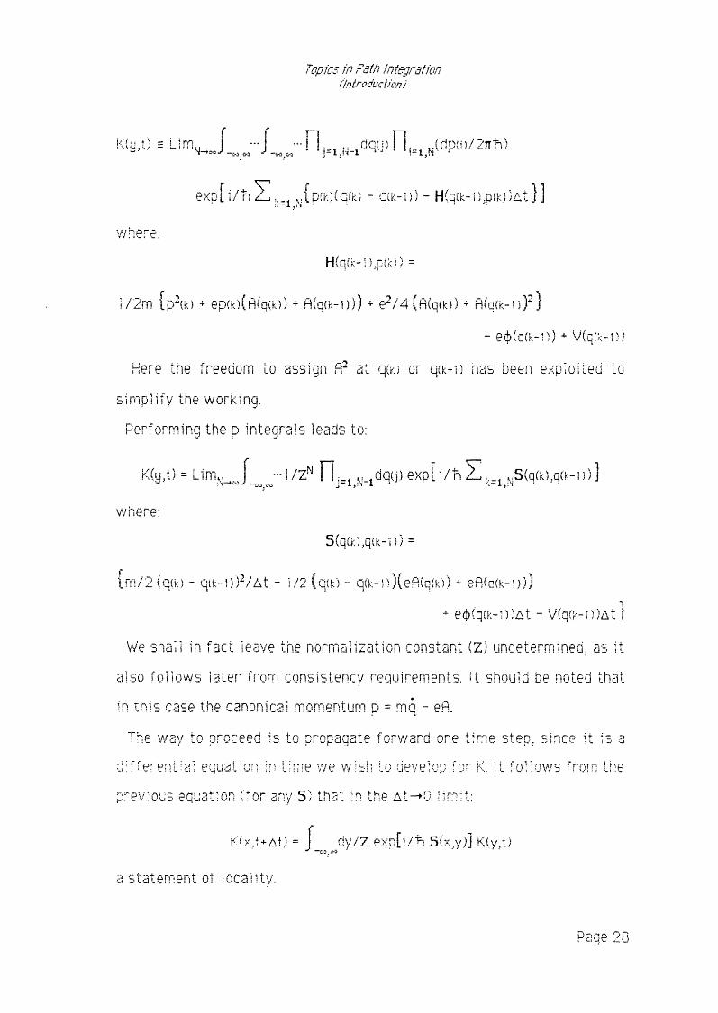
; / , i 4 ') — I ■; ryt= - lW'H I - j - F I - • .. , CiGU) f l . . ,:(dD(;)/2Jlti)

X p [ l / h X ; . vlp(k)(Gfk) - Q(k-I)) - H(q£k-1),p(k))At}]

wnere:

H(g(k- ; ),u(k)) =

i / zm {p “(ki + 6p(k)(H0q(k)) + H(qfk— i ).)) + 0 V 4 (fi(q(k>) + R(G(k-l)J*}

- e<j)(q(k-n) + V(q;k-n)

Here the freedom to assign R2 at q(k) or qfk-i) has been exploited to

simplify the workinq.

Performing the p integrals leads to:

!\(q,t/ = l iH I | "■ i / Z ] I ;_. v . CiQ(j) exp[ 1/ r z Li . . «.S Q{k),q(k-l) / j

where:

S(q(k),q(k-1)) =

im/2 (q(k) - qik-Dr/At - i/2 Cq(k) - q{k-p)(eFKq(k)) + eR(o(k.-l}))

+ e<j)Cq{k-1))At - V(q(k-D)At}

We shall in fact leave the normalization constant (Z) undetermined, as it

also follows later from consistency requirements, it should be noted that

In ihis case the canonical momentum p = mo - eft.

The way to proceed is to propagate forward one time step, since It is a

U’* fp^pnf 1e1 equation m t ’rqe we ywc-h *o neyplon Per K it *o"hnwc- frnm thp

pêwous equation Wor any 5) that In the At-»0 limit:

KTx,t+At) = I dy/Z exotl/ti S(x,y)] K(y,t)

a statement of locality.

Page 28

Topics in Path integration/introduction)

Explicitly, for the case in question:

K(x,t+AD = J ciy/Z

exp[i/h (m/2 {x-y)2/Ai - i/2 (x-y}(eft(x,t) + efl(y,t})

+ eA(y,t}At - V (y,t)A t)] K(y,u

woi Ki'iiG to oraer A l and se 111no c = x~y (recai! ^ y.

K f Y * 4- A * ! =. *• • * • j - *-* •• •* d f/z exp[i/h (m£2/ 2At)]J “'•lO t-2i

{ i - i t / n eH(x,t) - ip / 2 n edfi(x,t)/dx * ...

+ }/f\ 0(j)(X,t)At + ...

- i /n V(x,t)At - ...

- t 2/ 2 h 2 e2ft2(x,t) - ... ) (K(x,i) + dK(x,t)/*x £ + 1/2 d2K(x,t)/dx2 P + ... )

= 1 rif/z exp[i/"h (m£2/ 2At) ]

(! 5 - i/to (fefttx.U - £2/ 2 edH(x,ir/dx + epix.DAt - Vfx.nAt)

>•”> / 4. "V \ , .-eg i a. i h G rrv x, 15 j K( x, •. *

( f - :/ h £2e fiix ,:i) SKsx.n/i'x

_ . 7, . . v ^t / 2 K.f x, t) / o yp

Z is determined from the consistency requirement that

d -._j i 0 0 i l l 1 1 ” **J U i v-i C i . i . 0 .,

tfcJL I i

from which we oeouce:

j _ ot'/z exp[i/n (mf2/2At)]

Z = (2jii1iAt/rn)I/2

Pace no

Topics in Path integration(introduction}

a s L) 0 i or©, u v '• i

explias2] ds = v(m/a)

Performing the main integral using also:

f _ s2 exp[ias23 ds = V(m/a) (l/2a)

(odd integrals disappearing) leads to:

(K(x, At) - K (x ,i))/A t -

(1 /2m e3R(x,t>/dx - ie<j>(x,t)/ n - iVix/P/fi - i/2rn n e2R2ix,t}) Hex,!)

+ 1/m eP(x,t) dKtx/o/dx

+ In /2 iii 0“KaX, t) / 0 YC

in the limit &t-*0 we then obtain:

its d K / d t = 1/2m (its d/dx + efl)2 K - e * K + VK

Schrodinger's equation for a non-relativistic particle in the presence of an electromagnetic field

i he differentia] is correctly represented here since we are no longer

within the path integral. Had we not taken care of where R was evaluated,

additional anomalous’ terms would m general appear, the oath integral

Hamiltonian would then no longer correspond directly to that appearing in

in© to! responding Dohrouinger s eguation. i hese anomalous terms wuuid ue

responsible for spoiling gauge invariance, in summary, the mid-point rule

hides no secrets, and for this reason is favoured.

inis anarysis was true lor positive times ot propagation. Lnoosing r = 0

for negative times and investigating the snort time propagator:

5 anr^t-o-J ••• J ^ „••• f l jM N^dqij) n „ t Jd p ti)/2*Ti>

Pace 30

Tonics in Pstn integration (Introduction./

e x p i . l/ 'h S j^ N{p(k)(qtk) - qck-n) - H(q'k-n;p(k))At}]

For a short time of propagation, since the ‘time of flight' tends to zero:

we f;0pp only work to order (At) .

j L iN_,:dqfj) nWiN(H —-i r; 1 r^ 1 it

expt i/th 2 _j, v;{pik5(u(k) - u(k-n) - p~(k) At/Am}]

the oniy leading order term in the Hamiltonian being of the form p2/2mfq).

Setting you = q(k) - q(k-u this may be evaluated from:

lv = j - { u idu(j) I I • _. M(dp(i)/2 j!n)

P>;xp[ \/ft zL , =1 N{-p 2(k) At/2m 0{k)U(k)}]

— JC1* f % P . «•—. 4“- 0 ( M .O, L

for t by choice

from which it follows that:

iti dK/dt - H K = if* S(q-qQ) S(t-t0)

so that K is in fact seen to be the Green's function of the Schrodinqer

equation. This is consistent with the picture of a particle appearinq at the

space \ Cj C't 1 Pv T f"O'

i-’aqe o

Topics in Path Integration(introduction/

S VI Are all paths explored bg nature?

Fascinating is the question as to whether the probability amplitude wave

really explores every path (reference to a particle or localized object

should not be made outside of the act of localized interaction). This is

aptly answered by Feynman [1985] in a discussion of mirrors and

diffraction gratings. So intriguing is the argument that it is presented

here as an illustration of the insight offered by the path integral picture.

Consider reflection from a large mirror (a screen preventing direct

observation).

light x source

\\\

screen

I\ x

x detector/

/observed p-ath of reflection

rmrror

Reflection from a Mirror

We expect (from observation) in the symmetric case illustrated, for

reflection to occur from the middle, and not the ends of the mirror. 5ut the

path integral postulates that all paths contribute equally. The resolution

to this dilemma is contained in recalling that the classical contribution is

from around the least action path, so recovering the law of reflection that

Page 32

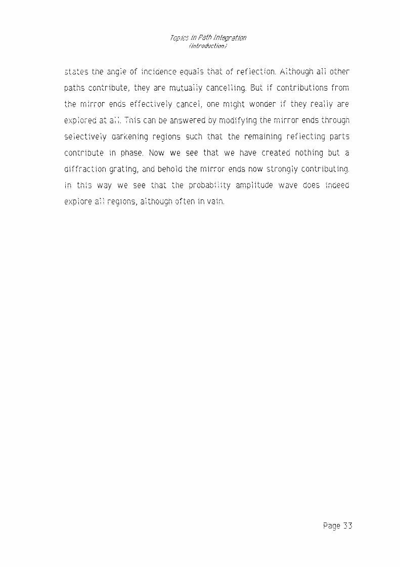
Topics in Path Integration(introduction)

states the angle of incidence equals that of reflection. Although all other

paths contribute, they are mutually cancelling. But if contributions from

the mirror ends effectively cancel, one might wonder if they really are

explored at all. In is can be answered by modifying the mirror ends through

selectively aarkenlng regions such that the remaining reflecting parts

contribute in phase. Now we see that we have created nothing but a

diffraction grating, and behold the mirror ends now strongly contributing,

sn tms Way we see tii a l the prouabi1iiy amuliiuUe wave

explore ail regions, although often in vain.

Pane 33

Topics in Path integration(Solenoid Scattering)

Q ap ier 0 ne

P-3G0 34

Topics in Path integrationf Solenoid ScoilennoJ

SI Introduction

this work a gauge free form

different! al cross section fc

ar particl es from a classic

explicit choice of a gauge. The result is found to agree with that obtained

through a gauge choice.

In the classical theory of electromagnetic Interactions (Electrodynamics),

as consolidated by Maxwell, one has physical fields. There is the

electrostatic (E ) field and the magnetic (B) field, which although a

relativistic manifestation of the E field, turns out to be useful to consider

In its own right. At this level (classical) it is calculatlonally convenient

to Introduce potentials from which the E and B fields are obtained. The

problem Is complicated in that although a field of potentials uniquely

describes a particular electromagnetic (E and B) field, the converse is not

true. This leads to freedom of choice as to which potential description one

chooses to work with (any one of a family giving the same physical

predictions). Naturally a gauge Is chosen so as to make the computation as

simple or illuminating as possible. But since any one of the family are in

principle equally good, one might suspect that a technique exists whereby

a computation could be performed without the explicit choice of a

particular gauge, in classical electromagnetism the use of a potential

field is entirely mathematical and in principle it need not have been

introduced (although it was for calculations! convenience); and so such

oddities as gauge freedom (and the associated need to gauge fix) might not

seem obiectlonable. The big surprise arrives with the introduction of

Page 35


quantum mechanics, where the potentials are introduced as a part of the

formalism describing charged particles, rather than on an optional basis

as before. The potentials here are no longer a mathematical option, but

they retain their gauge freedom: i.e. entire families continue to describe

individual physical configurations (This relates through Noether's theorem

to the conservation of electric charge). This inclusion of the potentials

leads to philosophical problems as to whether the potentials are physical

fields or not. In classical electromagnetism they were not directly

responsible for any physically detectable effect; as is clear from recalling

that this theory can be formulated in terms of the electric and magnetic

fields with no reference to the potentials. This is not the case for quantum

mechanics, where it was shown (by Aharonov and Bohm in their influential

paper [Aharonov and Bohmt /959; see also Kretzschmay /965]) that the

potential has a physically detectable influence. It Is in this sense that the

potential field is a physical field (it gives rise to physical effects). Yet

the potential field has an arbitrariness (gauge freedom); and this might

lead one to believe that it was still a mathematical artifact even in the

quantum theory.

The so called Aharonov-Bohrn effect [Feynman, I96JJ has been

experimentally confirmed and shows that the potential contains some

r\ ! 4-•Ji :-y O 1 U Ci i i eality, although gauge freedom speaks against It being the

physical field Itse‘

At present, most calculations are done having selected a particular gauge

to work In. These procedures, although valid, are not without associated

problems. In practice It seems that no particular gauge wins outright, one

with certain desirable advantages fends to have associated with it

disadvantages. Further it has been found by Feynman that the perturbation

Page 36

Topics in Path Integration(Solenoid Scattering)

expansion can be expressed in diagrammatic form with the possible

interpretation of particles interacting in different ‘ways. The contribution

of a particular diagram can be gauge dependent, which brings the above

interpretation into question. For these and other reasons it would be nice

(and should be possible in principle) to formulate a description of the

physics which, although still possessing gauge freedom (as It must), does

not require an explicit choice of gauge In making a prediction.

An excellent and extensive review of the Aharonov-Bohm phenomena has

recently been published fO/ar/uandPopescu, 1985] znd discusses in detail

the conceptual and experimental problems it broaches.

Page *7*7/

Topics in Path integration(Solenoid Scotiering)

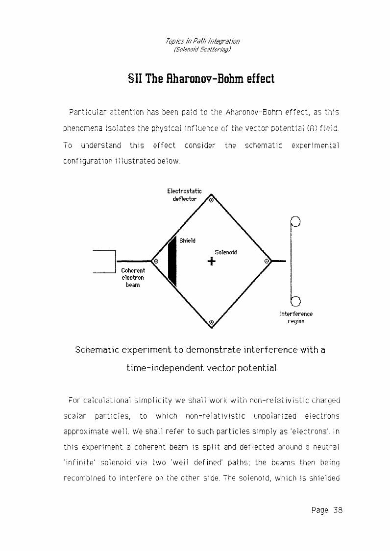
SII The flharonov-Bohm effect

Particular attention has been paid to the Aharonov-Bohm effect, as this

phenomena isolates the physical influence of the vector potential (ft) field.

To understand this effect consider the schematic exoerimenta]

configuration illustrated below.

Coherentelectronbeam

Electrostatic

Schematic experiment to demonstrate interference with a

time-independent vector potential

For calculations! simplicity we shall work with non-relativistic charged

scalar particles, to which non-relativistic unpolarized electrons

approximate well. We shall refer to such particles simply as ‘electrons', in

this experiment a coherent beam is split and deflected around a neutral

‘infinite' solenoid via two ‘well defined' paths; the beams then being

recombined to interfere on the other side. The solenoid, which is shielded

Paqe 38

Topics in Path integration(Solenoid Sootierinq)

from the electron beam carries a constant current. For such a solenoid the

magnetic field is contained within the coils. However, the vector potential

ft cannot be zero everywhere outside the solenoid because the total flux

through every loop is equal to the penetrating flux (#):

|ft.dl = f(^ ft).d5 = jB.dS = #

(by Stokes' iaw and the definition of R)

5o in this configuration the electrons pass through regions occupied by

the ft field only. This clarifies the situation by removing the influence of

the electric and magnetic fields on the electrons. We should now like to

calculate the detectable Influence of this ft field (if any) upon the electron

beam. Consider the motion of non-reiativistic scalar particles which are

described by the Schrddinger equation:

[(iht\)2/2M - fhdj \|/ = 0 (P2/2M = E)

If, to describe charged particles, we then demand that the global gauge

Invariance becomes local, we introduce the covariant derivative (minimal

coupling) Into the equation of motion:

itW -> i nu -*■ eft

where c = I In these units

[(ind eft J 2/2M - (i nek + eftt)] A = 0X X L l *

which as pointed out by Dirac, has the solution for the contribution from

the path p:

\y. i h p p p

- Xj/exptiS/ nj

5 = e lj rt ;n. u i

pCjflQ ~ Q


\|/ being the uncoupled (Tree field) solution.

this is in fact a result of the covariant derivative and does not depend on the particular-equation of motion

The integral being evaluated along the path p. This phase shift has a

physical consequence when the two symmetric paths interfere; for then,

adding amplitudes:

‘t 1 = XJ/expUSj/ n) + \|/exp( i5 /"h)

= \|/ exp [ie/th J R.dl] {! + exp[-ie#/1o]}

where # is the flux contained within the path loop. Then the

(experimentally observable) probability density is then given by:

!<&!2 = 4 iXj/!2 cos2(e#/2‘h)

which predicts an observable effect upon the interference pattern due to

the flux within the solenoid. This derivation is along the lines of that

performed by Aharonov and Bohrn [1959] in their original paper, and it

should be noted that the solution has been obtained without the explicit

use or a gauge.

Two further things are worth noting:

i) the effect Is lo s t 1 if the flux is an integer multiple of h/e; the Dirac

quantized magnetic flux (remembering that c=l in this analysis).

ii) the gauge invariant quantity jfl.dl is acting as the physically invariant

quantity. This quantity does not suffer from the same arbitrariness as R

itself, since it Is not dependent upon the choice of gauge (one need not be

Page 40

Topics in Path integration(Solenoid Scotierino)

made for ts determination \j.

This analysis serves to suggest important quantities and motivates

procedure adopted in the gauge free approach that follows. This wor

based upon a paper by the author [Shfekh, 1986].


Sill The Gauge free approach

In an attempt to clarify the mechanism at work in the previous analysis;

the same result has been rederlved from a slightly different perspective:

The following notation is adopted for clarity:

A lower case Greek character symbolizes the contribution to the field

from a particular path; while the upper case Is used for the complete field

at that point; l.e. the sum of the contributions from all paths to that point.

Starting from the field equation for non-relativlstlc charged scalar

[(i"hax + eftx)~/2M ~ (ific)f + - 0

The use of a gauge choice might be avoided if one could formulate the

above in terms of gauge Invariant variables. For this reason Mandelstam

[1962] Introduces the covariant variables:

X|/(p) = $(p.) exp[-ie/h J H.dl]

since such variables do not require a gauge choice for their determination.

The Introduction of this path dependent integral is motivated by the

previous analysis.

It should be made clear at this point that the Feynman path Integral

outmok [Feynman, i 943; Feynman anPH/PPs, /965] is being taken, where

the field at a point <J>(x) is the sum of contributions <jKp) from all possible

paths to the point x (see appendix I for a heuristic derivation of the path

integral technique).

That is:

Pace 40

Topics in Path integration(Solenoid Scatter inn)

<D(x) = 2 4(pP(LJHaving specified the path p, the end point is redundant.)

The derivatives on the path dependent Mandelstam variables are defined

in a natural way and are themselves covariant:

D^Cp) e LimSxii_.0{l|/(p’) - X(J(p)}/5x^

where the path p' is obtained from the path p by giving it an extension of

magnitude Sx in the [l direction (see figure below).

The path extension as used in the definition of the covariant

derivative on the Mandelstam variables

f chshould be noted that, like the usual covariant derivatives, the

operators D and Dv do not commute If there Is an electromagnetic field

present; explicit calculation

[D|1,Dv]X|/(p) = -ie/ft\)l(p)F UV

Page 43

topics in Path Integration(Solenoid Scattering)

wnere

jiV a ft - a p.}1 V V ^

Under Mandelstam's transformation, the field equations become

[(ihDx)2/2M - if)Dt] \|/(p) = 0

the advantage of this procedure Is that the Mandelstam variable XJ/ obeys

a 'free field’ equation of motion. The problem then breaks down into

solving for the free field contributions, and then inverting the Mandelstam

transformation in order to determine the original field contributions.

Because the result of any measurement involves only closed loops of

paths, the inversion procedure might be expected to involve only the gauge

Invariant quantity:

oft.dl

it is hoped therefore, by this procedure, to find the probability density of

the field without the necessity of specifying a particular gauge.

This technique Is Illustrated in the calculation of the Aharonov-Bohm

effect, as described previously.

Tine concept of a reference path will be Introduced at this stage, although

In this particular case it Is not necessary; but becomes convenient for less

symmetric configurations. When many paths are Involved it Is possible to

compare each against a chosen one, but In general none Is naturally

selected. The use of a separate reference path avoids this dilemma.

The configuration of Interest (with reference path) is Illustrated in the

figure below.

Pace dd

Topics in Hath integration(Solenoid Scattering)

Upper

The use of a reference path against which to compare phases

’he Mandelstam variable t|/ obeys the 'free field' equation:

[(itiD„)2/2M - ifiD,] \i/(p) = 0

Having solved for \j/ one9. thpn hrtS ie task of reverting back to this

procedure being path dependent.

For me upper path:

= XJ/ exp [ie/U U

^presenting the upper path; similarly for the lower path:

<|> = \|/exp [ie/h J.fi.dl]

but = \j/ (= \|/) from symmetry.

Now multiplying the field at each point by a unique phase factor does not

alter the physics (but completes the loops as desired).

It would not be admissiole to multiply by a m u ltiv a lu e d phase factor

Page 45

Topics in Path integration(Solenoid Scattering.)

(each loop to a given point must be compared against the same phase at

that point).

So, re-define:

4 =\|f exp [ie/n jU ld l] Up*

^ = *j/exp [ie/ti J ]n dl] UrB

where Up* is the (fixed) phase change along the reference path (see

previous figure):

U„ = exp [ie/n J fi.dl]

this is analogous to a choice of gauge; but this choice is arbitrary and so

unspecified i.e. an explicit gauge choice has not been made.

So:

$ = X|/ exp [ie/n | u-fl.di]

(the bar symbolizing the path reversed)

where this is the loop integral over the upper and reference oaths.

Although these path contributions are themselves multivalued, the total

Kernes shoiho be single vaiueo.

d ini 1 i sr ly:

= \|/ exp [ie/h pR.dl]

then adding oath contributions:

<|> = û i

= \|X ( exp [ie/n ^R.dl]+ exp [ie/h jp pft.dl] )

This kernel is not single valued (although its magnitude is). This is

because we have modeled a situation that cannot be set up even in

Page 46

Topics in Pdth in ityrd iion(Solenoid Scoiterino)

principle, since it is not possible to eliminate contributions from paths

that loop the solenoid many times. In this derivation, such contributions

have been neglected (which is a valid approximation if the path length Is

much greater than the De-Broglie wave length). If account is taken of all

possible paths; then the total kernel becomes single valued. This is clear

because, on looping the origin with the detector (by any path), each

contributing path is modified; but we still perform the same sum over all

possible paths.

The probability density Is given by:

j<&j2 = |X|/|2 ( 2 + exp [ie/ts Jy -,fi.dl] + exp [- ie /n <Jp -fi.dl] )

where the Integrals now loop over the upper and lower path and the

arbitrary reference path has dropped out of the formalism. Note that we

have not had to actually specify this reference path (which Is equivalent

to not explicitly making a gauge choice).

|<I»r = H|/i2 cos2(e#/2 ii)

as before, where # is the flux looped

All this work seems to indicate the adoption of the Feynman path integral

formalism [Feynman, 1948; Feynman and Hibbs, 1965] and it Is hoped that

within this context one might be able to continue in general to avoid the

explicit use of a gauge.

The work set out above suggests a natural extension. The original

Aharonov-Bohrn paper [(959] and a recent paper by Aharonov et al [1984

are concerned with plane wave scattering by an Aharonov-Bohm solenoid

(see also [Kretzschmar. 1965]). Both calculations make use of traditional

techniques with the associated need to make a gauge choice. It would seem

natural to try and rederlve their result for the differential cross section

Page 47

Topics in Path integration(So tenoid Scotterinq)

using the formalism presented above in the desire to perform the

calculation without the use of an explicit gauge choice.

It should be noted that the path Integral formalism seems to be naturally

adooted bv this techniaue.

Page 48


SIV notes on Scattering bg an Hharonov-Bohm Solenoid

ising the gauge free formalism (explained previously) the scalar field

implitude is given by:

0 (x ) = 2 \|/(p) exp [ie/n | R.dl]

(summing over 3 !! paths)

where \|/(p) is the free field amplitude contribution from the path p and

a ,-ni i .L i t

is the phase change due to the field R along the closed loop formed by this

and the reference path.

(These are in fact the Wilson loops of lattice gauge theory, which is also

a formalism that does not require an explicit gauge choice.)

it might be supposed that this phase change Is oath Independent (for the

'Aharonov-Bohm case') since:

R.dl = #

where # is the flux enclosed,

must oe considered i.e. paths

But it iiiUst ue remembered that an Datesr i 1

that loop more tnan once are included, ihe

phase change actually depends upon the number of loops performed by the

patn around the solenoid i.e.:

R.dl = m#

where m is the winding number.

So it seems natural to divide the above Into families of paths accordino

to the total number of loops made, it can in fact be shown [Laidiaw ant

DeWitt-fiorette, /y7//that the kernel must factorize in this manner i.e.:

Pace 49

0 ( X ) = 2 . \j/(pj) exp[ie/n Fl.U 1 ] (summing over one loop paths)

+ 2^ \|/(p .7) expjje/ n H .d i] (summing over two loop paths)

+ etC. (including counter looping)

Then for each individual sum over paths the phase change is constant and


u6 taken out.-

«t> = e's>lh I W(p,)

I 7\|/(p2)+ 0i2e#/Ts

+ etc.

leaving a set of path integrals, each of which is now a partial sum of paths

over the free field [Dowker, 1977].

It seems that drawing the distinction between n loop paths is very

difficult in Cartesian coordinates and calls for the use of cylindrical

polars [Edwards and Gulyaev, (964/ with their associated complications.

Then if the end point is at an angular coordinate 0; the one loop paths end

ai 0+2h. etc.

Page 50

Topics in Path Integration(Solenoid Scattering}

§ V Calculating the Differential Cross Section for Plane Wave Scattering from an Hharonov-Bohm Solenoid in the

Gauge Free Formalism

The calculation is performed for non-relativistic charged scalar

particles 'within a classical potential field.

The two dimensional, non-relativistic, free particle Feynman Kernel in

Cartesian coordinates is given by (see appendix I):

K = Urn _ (p/iJtAt)n n dxfki dy(k)

exp[ ip 2 n{ (xij) - x y - n r / A t + (ycj) - y(j-i5)2/At } j

where:p = M/2 T)

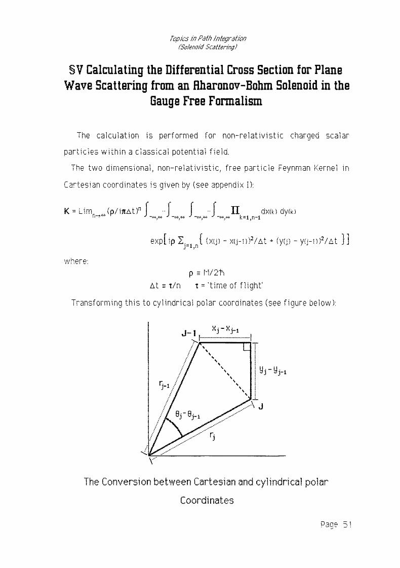
At = t/n t = 'time of flight'

Transforming this to cylindrical polar coordinates (see figure below):

iae

The Conversion between Cartesian and cylindrical polar

Coordinates

Topics in Path Integration{Solenoid Scattering/

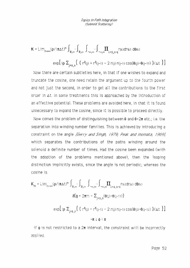
K = Lim„ (p/1nAt)n j ••[ f f II iJ o,*> J o}~ k= i,n-i

rCk)dr(k) deck)

exp[ip 2. f ( r2(j) + r2(j-n - 2 r(0 r(j-n cos(8(j)-8(i-i)) )/At 1]j - i ;n

Now there are certain subtleties here, in that if one wishes to expand and

truncate the cosine, one need retain the argument up to the fourth power

and not just the second, in order to get all the contributions to the first

order in At. In some treatments this is approached by the introduction of

an effective potential. These problems are avoided here, in that it is found

unnecessary to expand the cosine, since it is possible to proceed directly.

Now comes the problem of distinguishing between 8 and 0+2ji etc.; i.e. the

separation into winding number families. This is achieved by Introducing a

constraint on the angle [Gerry and Singh, 1979; Peak and /nomata. 1969],

which separates the contributions of the paths winding around the

solenoid a definite number of times. Had the cosine been expanded (with

the adoption of the problems mentioned above), then the looping

distinction implicitly exists, since the angle is not periodic; whereas the

cosine is

!< = Lirn_ (p/mAt)n •• •• II nkidnum k=i,n-I

d8(k j

(p + 2nrn - 2. (8cj)-0Cj-!)))• j= i,n J

exp[ ip 2 n{ ( r2(j) rdj-i) - 2 r(j) r(j-n cos(6(j)-0(j-u) )/At }]j *ii:

-n i 0 < ji

if 0 is not restricted to a 2n interval, the constraint will be Incorrectly

apo lied.

aoe n?

Topics in Path integration(Solenoid Scattering J

A :trick1 is used to place the constraint into the exponential [Edwards,

I967hirdd\ the Lagrangian by using the relation (which follows from

Fourier exoandina):

2jiS(x ) = J _ e!Xx dX

) d0(k)K = Limr (p/inAt)n I ••) f f II rckidrtkm n-*«s'r J o,c* J 0 J k=l,n-l

1/ 2n \ eil<* + 2r,m! eft.

II sxd [ ip ( r r j ) + r n - n - 2 rm n > n co s(0m -0{j-i)))/A t -iX (0 (n -0 (j-n )]j=i,n

-ni§in

Using the transformation:

^(i) = Q(j) - 0(j-n

for which the Jacobian is unitv.

K „ = Urn, (p/iiiAt)n - II H'kjdr(k)H n-*« r ■ ' 0,** J Q,i* k=i,n-i!/ 2n I eaU + 25im)dX II. exp[ip(r2(j) + nj-uVAt]

f •• [" II dY(i) exp[-Uip( r(j) nj-i) cos(yfj)) )/At ~ IayO) ]-• -s.R !=i,n-i

Asymmetric angular limits 0—2n are incorrect, since they compel the

path to circle in one direction, but not circle back.

The angular integrals may be performed using the asymptotic relation

(for |zi-*Q°) [Gradshteyn andRyzhik: P958Prom 8.881(5)]:

f e ,*x+ z C05lXJ 6y -» 2 n L . ( z )J -n,n v !*■!

paqe 5J

Topics in Hath Integration(Solenoid Scatier/nc//

larg z! s n il

It should be noted that this limit is achieved when going to the continuum

(At-*0 ), and so an approximation Is not being made at this point.

it Is this step that allows us to proceed without expanding and truncating

the cosine.

K = L!mr (p/inAt)n •• II r(k}dr(k)m r k=i,n-i

JA.(o + 2?tm} dA

II exp[ip(r2(i) + r2(j-n)/At] 2flL ,{-ip 2 ru)r(j-u/At)j=i,n M

.ookinq at the r integrals:

I = Urn (2p/iAt)n ••] II nk)dr(k)n- « r -'oJ« ; 0.« jf=l,n-l

II exp[ip(r2(!) + r2(j-i))/At] L.(-ip2r(j)nj-i)/At)j=i,n

Explicitly

I = Limn . (2p/lAt)n I •• r.(k)dr,(k) r_(k)dr.(k)... r .oodr jk)n-?« r ■> J 1 1 2 2 n-i n-1

exp[ipR'2/At] exp[ip2r12/At] exp[ip2r22/ A t ] ... exp[ipR2/At]

I!X|(-ip2RT1/At) Iw(-ip2r2r1/At) Iw(-ip2r3r2/A t) ... Iw(-ip2rn. 1K/At)

iv. i b ilUW UUib i L: i 0 i.0 pi UL00LJ U o C Ip lO0 i (J0H v. I <_ [uradh/li tryH CtflU liy^L/!ft\,

P7/G from 6.61!]:

f expilom2] L(- iar) L(-ibr) r dr = i/2a exp[-i(a2+b2)/4a] l,(iab/2a)Q rv A* Ad

(Re A > -1)

by which the r integrals may be successively performed to yield:

Page 54

Topics in Path integration(Solenoid Scatterin'])

K « p/ijn exp[ip(R‘2*R2)/t] | dX ew * + 2l!m) L.(-2iR'Rp/t)

where t = ‘time of flight

Applying the gauge free technique as described previously we sum over

all possible winding numbers before doing the X integration:

K = 2 JemJf/T? K

K = p/int exp[lp(R,2+R2)/t] J dA 2 e2R1,mft ^2ftiTi) i (-21' c-i-j j <Ti — £-3,fr3 r - |

where a = e#/h

Using the Identity:

2 eim9 = 2Ji2. 8(8 + 2nn)m =- n=-

WiiiLH Tuliows from the Poisson suni formula, wnich itseii derives frorn

rourier ana«ys is.

K = p/iUrr exD[ip(R'2+R2)/x] 2 e-i(n+cO* t (-21R‘Rp/T)1 1 * p=-m n+ai *" i ~ '

Now note that:

Leading to:

I C-ix) = H ) VJ (x)v V

K = p /iE T exp[ip(R'2+R2)/t] 2 e ,(n+a)* ( - 1)ln+eti j (2R'Rp/x)r * n=-*aJ» jn+aj ’

where:

p = M/2 n a = e#/h (c=l)

“31 i 0 < 71

The non-relativistic scalar kernel for the needle solenoid

this Kernel /Dowses !977i although single valued, as It must be,

Page 55

Topics in Patti integration(Solenoid ScotiorinQJ

discontinuous in phase. This is due to an implicit insistence that on

looping the origin with the detector, the reference path must be restored

to that originally used to that point, (i.e. only a single gauge be used at

each point). This requires that the solenoid be cut by the reference path

and leads to the discontinuity. Since this discontinuity exists only in

phase, it is not reflected In the physical predictions.

We have here linked up with the solution to the differential equation, but

what takes a few lines for that technique [Aharonov and Bohm, (959,

Kretzschmar, 1965] has taken us longer.

K = p/litT exp[lp(R'2+H2)/t] 5(2,5'Rp/T) e ,ct*

wnere:

5 (s ) = I p-'1*in+«|'

Mow we are at liberty to multiply by an overall single valued phase

factor (for the reasons expanded upon previously):

pik$

where k is an integer, in order to work with a new a that lies in the range

0<a<l. This is a matter of convenience and illustrates the periodic

benavior In oc (the rescaled flux strength).

Following the work of Aharonov and Bohm [1959] we choose to split 5

into three parts; so that the absolute value sign may be removed:

S ~ ^ + S ■+■ Sw w-2 w 3

y.mppp-

c _ > / _ i \n+ct i (r-. \ Q-na• > - \ ~ 1} a {=} i t?I n=l,« n+c*

S = 7 f - i lin'-'«! ,1 {c ■> o-in*'J2 irru' ~

Page 56

To/y/cs in Path integration(Solenoid Scoiterino)

= 2 H ) nH J (s) e™*n=i,« n-a- _ i i \a i}_ - \ ~ } ) u . k h i 3 u .

We now construct and solve for a partial differential equation satisfied

by Sj [Aharonov and Bohmf 19591 In this way we evaluate the sum for 5

(S, follows from 0-*-0; o

b S . / d s = 1/2 2 (-i)n+t< ( J (s) - J , (s ) ) e'in*i f|=i ca n-tot-1 m-otti

navi no used

fi ’ <•-) / fie = ■ /v f j ! c,) - ] f c ) )u -y 3 j ^ ,Jv-1v 3 ' ‘-'V+ r *

V - 0

yielding a finite term partial differential equation:

bS./'ds = -i cos0 5. + 1/2 H ) “ f J As) - i J (s) e-10 )

which is of the form:

d5(s,0)/ds = p(s,0) 5 (5 ,0) + q(s,0)

and has the solution:

5(s,0) = exp[ J(s,0) ds 3 { J _q(u,f) exp[- fHp(v,0) dv] du +f(0) }

where f(0) Is an arbitrary function. Hence:

5 = ; 1 2 (-j )a p~iS C05$ \ Qiu cos$ ( J (y) - : J (y) ) fjy 0,1 • ct+i

The lower limit (and arbitrary function of 0) being determined by the

■equirernent that when s goes to zero, 5, also qoes to zero because 5,

includes Bessel functions of positive *order r-.r, }\, T'«1r f n p cu i i! y. i i i i D i UI i 1 1 i •

superior for numerical eva luatlon than the 1;nflnite sum, which

fpom sio\n convergence for 1arge Bessel functlc)n argument.

'i 1


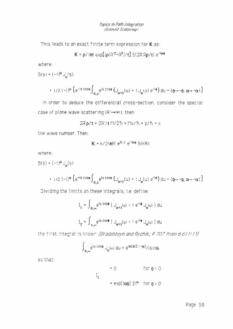
This leads to an exact finite term expression for K as:

— rt / i 'ff'T a -./nF' 0*24- -04 ' C" (’ i pv ■ i j . /.* i j-, ice“ p/ I JET b A p L i p ' O r\ ji i j u s i .H K p / 1/ c

w here:

5(s) = (-i)GJ (s)a

+ 1/2 (-l)K {e~:s C05§J elucos? ( j . .(u ) + I J (u) e_i ) du + (p-f-0, a-^-of)]J 0 15 tt+i ft r -

In order to deduce the differentia] cross-section, consider the special

case of plane wave scattering (R’-+oo); then

2R'p/t = 2R’/ t M/2 n = Mv/lh = p/ n = k

the 'wave number. Then:

K = k/2mR' e!k-K e“!G§ b(kR)

where:

5 ( S ) = ( - i ) « J (s )

+ \I2 i-\f- (e~ls cos$ f eiU cos* (J (u) + 1 J (u) e 10) du + (p-^-p, a-> -a )}JQ,s'' 'w«+lDividing the lim its on these intearalsj i.e. define:

I, = | eiu cos* f J ,(u) — i e J (u) I du1 j o,« ' a

, j e iu cos* (• J (u! _ j e-i* J (u) ] du4 ■'5 m CtTl ft

the first integral is known [Gradshteyn andRyzhik; P 707 from 6.61 H !)]:

J 0 !u - 0 3 $ j (u) = e m(?J2 - !^fVisin(tjtJ 0,« «

C 3w ui icu L.= 0

expMapj oP for p > 0

e Dd

where -n i 0 < n

Topics in Path integration(Solenoid Scattering}

•;ow iOOKinq at 1 ;

u = eIU C05* ( J .(u) - i e~'- J (u) ] du« et-f-1 ot

n the asymptotic lim it (z->«):

Ja(z) -* 4i2/ni) cos(z - m/2 - ji/4)

I, v ( 2 /n) [i + e ' ] (-j)“+3/2/V’( i + cos0 ) f rr expMz2] dz“ ri 1 S \ i + C O S $ > j

v(v/n) [ I - e 1$] ( + i)tt+3/2// ( I - cos0) I „ , , exot-iz2! d;' J V t s ( 1“ C O S0) J , « '

where we have put:

z = v[u(I + cos0)j in the first integral

z = / [u( 1 - co50)] in the second integral

Using the asymptotic behavior for the Fresnel Integrals [Gradshteyn anc Ryzhik; P 952 from 52551:

I expMz2! dz

exp[-iz2j dz1 ,j 3,

i/ 2 a expl+ia*\)

■ i Avnf.i \1/ w\(JL id j

Putting this together:

-V (- i/ 2Jt) { i e 15/Vs + e15/ v s cos(m + 0/ 2 )/cos(0/ 2 ) } +

There remains the contribution of S3, whose asymptotic behavior is:

( - I r f y s) ->■ (-i)G l(2/n$) costs -

-.pnrft-

u^no SQ

m / 2 - n/4)

Topics in Path intepration(Solenoid Sea tier (no)

C; . Q i ( « A - 5 C O S $ ) _ f t i / Q - . - N - j s ; r ,nu'zns) e13 simna) e+,*/2/cosu&i'i

Qn finoUww’ w t 11 i u i t y .

K

k/2mR' e!K-x e !a* { "kR cos - V(i/2nkR) e1KK sin(iEOt) e+,#Q/cos(0/2) }

f-Kg gpgnnd fpprn r pptps pntinq the scatfprpd vv vp frorn which ws r 0n

deduce the differential cross section:

d o / d $ = l /2nk sin2( * a ) / c o s 2($/2)a = s S i h

# = flux in solenoid k = wave number

it shouid he noted that this yields an infinite total cross section. This

reflects the fact that the effect is not dependent on loop size (which is

true only for the infinitely long solenoid).

Page 60

Topics in Path integration(So/enoid Scotterino)

Conclusion

Through the development of a gauge free technique, and the use of the

Feynman path integral method [Feynman, 1948; Feynman andHfhhs, 1965.J,

the differential cross-section for scattering of non-relativistic charged

scalar particles from a classical Aharonov-Bohm solenoid has been

determined. The result agrees with that obtained by Aharonov and Bohrn

[fQ5Q], but the calculation differs in principle, in that. It was no longer

necessary to make an explicit choice of gauge; although one was

implicitly made In the use of an arbitrary, but fixed, reference path.

The gauge free approach adopted here obliges one to use the path integral

formalism, since there is not an explicit potential for which to state

Schrodlnger ‘s equation.

Pane 61


Appendix IDeducing the Feynman Path Integral formalism directly

from the Probabilistic Wave description.(a heuristic approach)

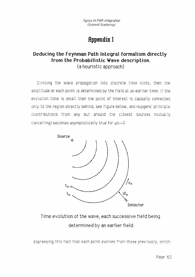
Dividing the wave propagation into discrete time slots, then the

amplitude at each point is determined by the field at an earlier time. If the

evolution time is small then the point of interest is causally connected

only to the region directly behind, see figure below, and Huygens' principle

(contributions from any but around the closest sources mutually

cancelling) becomes asymptotically true for At-*0.

Source

Time evolution of the wave, each successive field being

determined by an earlier field

txpressinq this fact that each point evolves from those previously, which

Pace 62

Topics in Hath integration(Solenoid ScoiterinQ)

are themselves determined by their own previous field:

O oc Jdxt exp[1k1.dii ] Jdx2 exp[ik2.dl2] ... Jdxn exp[ikn.dln]

This procedure Is nothing more than summing over all possible paths.

O = M l 1 expii f k.Gl]p V P

:t Is not suggested that a particle follows these paths, but rather the

paths should be considered only within the mathematical framework as an

alternative description of wave propagation, invoking the correspondence

principle, which te lls us how a particle's properties are related to its

wave nature gives:

= M l 2 exp[i/n (Jp.dx - J e dt) ]

*l> = M l 2 exotl/ti f(o.x - H)dt ] p ‘ J 1

with suitable provisos for when the Hamiltonian equals the energy.

<1* = 1 /Z 2 exp[ 15/th]p

where 5 is the Action

The path integral technique of Feynman

For non-relatlvlstlc particles in free field the action is simply:

5 = M/2 f[v 2 + v 2] dtj ' a y

u / ;- U r h | ! c p ; i in H i c r r p l u fArn-i i n f h p f p v ^ i J u j C U i i i u i j ' w l Ci-Vw i w i l i t i l l L i i C l C A l .

K = L1mrrt0O! /Z J _ ^ J ^ J ^

exp [ip l . _ t { (xfj) - x(j-n52/A i + Cyij) - ysj-n)2/At }]j —i , n

where p = n / 2 lh

The normalization constant (Z) may be determined (up to an overall phase

Paqe 63

Topics in Path integrationfSolenoid Scattering)

factor) by the requirement that the particle be detectable somewhere, i.e.

.. 1 . , K d '<“Cru.Cri^ .

This is so since the possibility exists of bringing together the dispersed

wave such that the magnitude and relative phases from each point are

maintained. This Tensing’ allows the amplitudes to Interfere before the

act of localized interaction. That this is different from the usual is

explained by the fact that the kernel gives the amplitude for the particle

to be found at a point and not the amplitude density usual to the 'wave

function. Performing the Gaussian integrals leads to:

1/Z = (iiiAt/p)~n

}! IL (p / iH A t)" ! - I i , . , ; L j l - i . m * ' ' d'/(n

exp[ ip 2 . { Cxij) - x(j-i))2/ A t + (yen - y(j-n)2/At } ]j—i j n

wnei 0 p = i ' i i l n

The free field non-re!ativistic scalar kernel

It has been implicitly assumed that we are working in flat space without

a velocity dependent ‘potential’ term, in general the normalization factor

Is path dependent [DeW/tt-Norette} /95/].

Pane G4

Topics in Path Integration(Solenoid Scattering}

Appendix I!A look at the controlling function (regulator) for

indefinite integrals

Many of the identities quoted depend on the evaluation of oscillating

integrands, which are made well defined by regulating the integrand and

then removing the regulator at the ends.

For examole:

i — L i i l i ft-MO1 L —p-ttt ,-ii-0

(a oositive)

This procedure can only be reasonable if the result Is independent of the

choice of regulator. Although expected on physical grounds this is not

altogether obvious and Is investigated below.

Consider integrating such a function along a closed path in the complex

plane. The first section of the contour* Is taken as the oath (along the real

axis) of the original indefinite integral and extends to infinity. The

contour is then continued off the real axis 'at infinity' to anv point in thei i *

complex plane where the unregulated Integrand is Itself suppressed to

zero. The contour is then completed from this point, by a return path, back

to the starting dace.

Hace bn


Evaluation of an oscillatory integral by means of a general

reaulator

Now if any regulator is chosen such that the contribution of the path

section at infinity is zero (such a regulator being referred to as ‘good' and

being determined by Jordan's Lemma), and if no poles are enclosed by the

closed contour; then by Cauchy's theorem, the integral pack along the

return path Is equal to the original Integral. Since this new integral Is

Independent of the choice of 'good' regulator (the Integrand itself now

achieving regulation and the regulator not contributing); so it becomes

clear that without obstructing poles the result of regularization Is

regulator independent.

Page 66

Topics in Path integration(Wedge Diffraction)

C L p ter T WO

i o f h In ie p r a J a p p r o a c h /<

r ! \\ a systematic aoDroacft/

/ i i

based on a paper byi

C.DeWitt-Moretts, S low , L.Schulmsn and A.Shiekh, Found ofPhys, 1 6 : (1986), 3!

(contributions by DeWitt-MoreLle, Low and Schulman stand independently and nave not been included)

Pace b 7

Topics in Path Integration(Wedne D inrjctionJ

SI Introduction

i this work the path integral technique is used to calculate the

inaction patterns from an impenetrable (perfectly absorbing or

perfectly reflecting) wedge for non-relativistic scalar particles and light.

An interesting connection with the Aharonov-Bohm effect is used to help

obtain these solutions. Time dependent kernels are developed for

non-relativistic particles, but only time independent kernels are found for

light. New forms of the solution are also presented, which overcome the

slow convergence problems of former exact solutions.

Sornrnerfeid in 1895 solved exactly the problem of the diffraction of

light from a perfectly reflecting wedge.

The same problem had been solved in electrostatics by solving Laplace’s

equation:

V2u = 0

ror a doint cnaroe outside of a two dimensional wedqe. For a conductin

v A! phnQ of external ancle n/v (v beinc a positive inte fjpr ) the boundary“**“£;**■ o "* ‘ ‘f ■;U If'* {Ui L 1ons u=0 may be imp lemented by the usual method of incages, images

hoi .n rnL/ V. i . !Cf Ufaced such that the boundary conditions are achi ever! K\ ! f~\ ;ro fr- a f r\ •'y y, i . 1: i e u y.

ThiQ fp-chnique fails for a general angle, as the images

the physical region outside of the wedge.

This difficulty may be overcome by means of a conformal transformatior,

a technique developed by Riemann in his doctoral thesis.

Since any analytic function:

W(z) = Ufz) + ’ V(z)

Rage 65

CCl

Topics in Path integration(krdge DifTrjri/on/

satisfies Laplace's equation by virtue of the Cauchy-Riemann conditions

i.e.

dU/dX = dV/dV dV/dX = “dU/dV/ i

One may transform the original configuration by the map:

7 = r 7'iL. i \ i /to another that w ill automatically satisfy Laplace's equation

d2W/dX2 + d2W/dV2 = o

W(Z) = U(Z) + i V£Z)

wherever the map is analytic.

Then solve this new electrostatic configuration for U (V follows from the

Cauchy-Riemann conditions) and transform back to determine the potential

chat Is a solution to the original problem.

The transformation:

7 =

may be used to turn a wedge of external angle [jut/v (jt,v being positive

Integers), into the tractable wedge problem of angle ji/ v .

m anstorrninq bacK yields a many-vaiued solution which is unuersioou <_o

ij e ihLe; pi 9 l8U m tne physical region outs ice or tne wedge.

Tne analytic d inicu sties or nidny-Vdiued rune Lions may dp overcuiiie oy

inr.roQucinq tne icea or a Kienianman surface \descr!den in apdend]x i). in

this oicture it becomes clear that the images do not lie in the physical

soace, but are 'hidden' in tne lower folds and act only to implement

boundary conditions.

From the analogy with suen problems in electrostatics; Sommerfeic

/ 1896J proposed a many-vaiued anzatz, which satisfied the Helmholtz

Q n i i i r , r v t v - U Ci l i KJl \

Pace 69

Topics in Path Integration(Wedge Diffraction)

[eO/uR" + i/R o/dR + i/R2 dr/Utjr + k“] G - ~5(.R~k ') 5(O~0 )

as well as the condition of no incoming wave from infinity. Here we have

converted to rationalized units and continue to do so. in this way he

deduced the (free re lativ istic massless time independent scalar) Green’s

function on a |i sheeted Riemannian surface as:

G = ; I2n 2 ^n-0,~ !

w nere:

! / • . r\ 'i , l K R n/ji

\ .-,-irtn/2U i/ ! ;;,rv i t p K , il-'.K

n/li

V2/jl for n>0

II 1 /|i f or n=u

k , iif R < R. interchange R and

3iRV/2 ( ,j _ Q-iv»j (....j- 1 “ ~v'A ’ ~v

k wave number

This, with the addition of suitable image contributions, satisfies the

wedge boundary conditions. In this way it Is possible to describe

diffraction from an impenetrable wedge; be It reflecting (with Dlrichiet or

Neumann boundary conditions), or perfectly absorbing.

Sommerfeld in his original paper fully develops the solution for the

reflecting infinite half plane. Carslaw//P/P/under his guidance completed

this task for the wedge, having earlier f/9/0j solved the diffusion

eguation v and so Schrbdinger’s eguatlon) for the we doe of any angle.

Mac Dona I d [1902]. in his Adams prize essay, developed the same results

for the Dirlchlet wedge by finding a solution that obeyed the Helmholtz

equation and the desired boundary conditions. He obtained the Green's

function (here rationalized):

70

Topics in Path integration(Wedge Diilruction)

-j

Gy. ~ ii/6 rLt 8xpl—in?r/ ,z0 j vkk j ~ikK / siiu.iiitd/9) sirunjuj) /6

tor R ’• R., uf k k interchange R anc R j

i w i BUfiidnn W8dQ8 is:

G / = 1/8 l J Q(kR) KQ(—IkK*)

'l 2 expHnrVzie] J nftfe R) K ^ C -lkR 1) cos(nj?q/8 ) cos(n5io78) j

for R < R’j (If R > R’ interchange R and R’l

these results are rederived here, in a constructive fashion, using the oath

integral technique of Feynman [Feynman, i 948; Feynman and Hihbs, 1965}

Page

Topics in Pdth integration(Wedpe Diffraction)

SII Path Integral Approach

It has been realized by L.S.Schulman and C.M.Newman (private

communication) that diffraction from an infinite half plane (see figure

Diffraction from a half Plane

can be related to the Aharonov-Bohm effect for a needle (infinitely

narrow) solenoid of infinite extent.

a needie

» - f l l i v

lo bee this unoovioub connecticm? consider scattering from

solenoid with strength a= i/2 (a the rescaled flux = e#/h; where

within the solenoid). Now one can gauge away the potential R at all points

except for a branch cut and so have a zero fie id except along this line (see

r s oure oei o w ).

Paqe


Location of Solenoid and associated Branch cut

Tne probability amplitude K(«= 1/2) to detect a particle changes by a phase

factor exp(in) when the detector crosses the line of non-zero potential, if

one then adds the kernel K(«=i/2) to K(«=o), one achieves mimicing of a

system with no penetration through the line, since the detector on passing

this line has half the iota! amplitude change sign, which k ills the total

kernel.

The complete normalized kernel for the edge, K Is thus given by:

K0 = 1/2 (K(«=1/2.) + K(e=o,0

Since the combined solution satisfies the free field equation, except on

the line, ana does not allow penetration of this line; one Is In this way

modeling a perfectly absorbing half plane carrier In free field. It should be

noted that a path that passes through the barrier and returns, has Its

Influence restored. This Is a weaker condition than demand I no that any

patn that passes through the barrier should not contribute.

ij snp » “7T

Topics in Path Integration(Wedge Diffraction}

image sources may then be introduced to model a perfectly reflecting

barrier. This is an extension of the normal method of images and is

discussed in more detail later

Alihough use was made of a special gauge to conceive this technique, the

solution itself, being gauge independent, tells us that, given a fixed source

and a fixed detector on each side of the barrier, the orientation or

dispersion of the barrier Is Irrelevant.

The complete non-relatlvistic scalar kernel can be readily deduced from

the expression [Morandi and Nenossi, /9S4J for the kernel for the

Aharonov-Bohm solenoid in two dimensions; namely from;

Kagj p/'ijtt exp[ip(R2+R'2)/t] 2 ____ (-i)>n+a’ J.^^R'Rp

-JtStjKJl

(or any 2a interval)

where p s n / 2 n

M scalar particle masst time of flightR distance from solenoid to detector R' distance from solenoid to source

« rescaled flux = eff/h; s = flux within the solenoid e scalar particle charge $ angle to detector y angle to source

and c= i in the chosen units

yielding

K g = p/1 jit exp[ip(R2+R’2)/t]

1 1/2 J (zR:Rp/t) + 2 ( - i m 2 J (2K'Rp/t) COs(n(0-0')/2) }u n=i,»

Now using the identity[Gradshteyn andRyzhik, f980; P97JProm 8.5/f(5h

pggp / Ci

Topics in Path integration(Wedqe Diffraction)

(a particular case of the Identity developed in appendix III)

!i'i J _ ( z )+ 2. H )n/2 J J z ) cos(n0)0 n=l M n/2n=i,«

= / ( I/ in ) e~izCO5{20) f , , exp[is2]ds■'-«IVt2z)cos(0)

anci recalling that p = M/2 h (M=scalar particle mass)

Kp = M/2;jTht exp[lM(R2+R'2)/2 nt]

J ( ] i \ n ) p-i(RRM I W cos(*-* ) | p v D i iq 2 ] rj,-J -« ,V (2K ’RM/Trt} c o s ( { $ - f y 2 } ‘

-jicijKn

The Kernel is divalued if we consider aM o To ronsfnict the probability

amplitude in the presence of a perfectly reflection barrier It Is

enlightening to consider this extended (analytically continued) kernel on a

two sneeted Riemannian surface (see fiaure below).

Topics in Path integrationfWodge Diffraction)

A short discussion of the use of Riemannlan sheeting instead of branch

cuts is given in appendix I. in this description the kernel is again

single-valued, and one of the sheets is taken to represent the physical

space. On such a surface the absorbed wave descends into the second

sneet, ratner than terminating upon crossing the barrier (as before).

Bcunoary conditions are implemented using the methoo of images

[Sommerfe/a 1954]. The physical configuration may for convenience be

considered to dwell upon the top (0 - 2n) sheet, while the image is 'hidden'

on the lower (2n-4n) sheet, which only influences the physical space in

implementing boundary conditions. In this way it Is understood that the

solution Is to be interpreted only upon the physical sheet.

To model a perfectly reflecting edge an image is Introduced at the

position, on the other sheet, obtained by reflecting the source In the

boundary wall. Dlrichlet boundary conditions (the total field K=0 on the

boundary) may be achieved by adding an image of equal amplitude, but In

antiphase with the source; while Neumann conditions (3K/3n=0; where n Is

the normal to the boundary) are achieved by having the Image run m phase

with the source.

From this one may deduce the non-relativistic scalar kernel for a ha'f

Plane Parmer (edge), with Dlrichlet(-) or Neumann(+) boundary conditions;

-espectweiy, as:

K .r = n / 2 mnt exp[iM(R24-R'2)/2nt] / ( l/ijt)

ri e /nt) cos($-$‘ )

,-/(2P.'P.N / nt) C05\t>-$ V2)expils2] ds ± (0 ->-o ) ]

where O' is the angle to the source and p is the angle to the point of

detection.

Topics in Path integration(Wedge DitTr-e/cUon)

Note that the barrier has been placed at zero a?

Note also that the kerne] for the reflecting barrier does depend upon the

ocation of the barrier, since this determines the image positions.

The above results agree with that obtained by Schulman [1982, fQ82J

Pane 7 7

Topics in Path integration{Wedge Diffraction)

§111 Generalization

A natural progression of this work is to rnodel an impenetrable wedge of

external angle 8 (see figure below).

Diffraction from a Wedae_r*

in order to do this, one would again like to use the method of Images to

implement the desired boundary conditions upon the two edges. This

suggests the introduction of image sources at the two positions obtained

by reflecting the source in each boundary wall. However, this does not

quite achieve the desired result, since an image placed to achieve a

boundary condition for one of the "aces w ill disturb that of the second. One

c sn cori_ect or this by adding v jrth e r images to restore these conditions.

Thus leads to images standing at 0= ± O’ ± 2k$; k an Integer (see figure

Pace 75

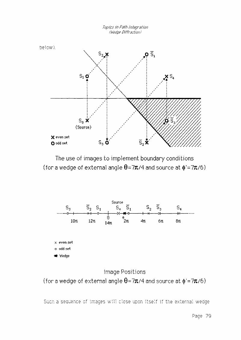
Topics in Pdih intearstion(Wedgs Diffraction)

The use of images to implement boundary conditions

(for a wedge of external angle 0=7ji/ 4 and source at

S3 S2 Sj S0 Sj s2 s3 s4---- O j------ JH o----1--- X —*-Q------ 1 5k£----ol-------- |X-

0 8iOn 12ti 2ti 4n 6ti 8fi

x even set

o odd set

Wedge

Image Positions

(for a wedge of external angle 9=7ji/ 4 and source at <j>'=?Jt/6)

u t: ! - —J . ; i i—iCJ w 'wJUUl lUw :olf if ff>o avfp rnq l uiorlnp) u i i i i l i i'v. v / s u C l i i u i Vv w ' u \ . j C

Paae 79

Topics in Path integration(Wedqe Diffraction)

angle is a rational number times n i.e.:

6 = Jiji/v

H,v positive integers

The image positions, which are conveniently grouped as those obtained

after an even number of reflections and those for an odd number (see

figure), are then Given respectively by:

R = H0 = <D* + 2Jik [i/v

and

R = R‘0 = -0' + 2flk [i/v

k = 1 ...V

This use of images, with the need to nide them, requires the

consideration of a [)- sheeted Riernannian surface; [l sheeted since the

Images close upon themselves after [t turns.

It is these considerations that motivate us to consider amplitudes

defined upon a fi sheeted configuration space; in the manner of Sornrnerfeld

[/8Q6, 1954] So a wedge of external anqle nji/v lives on 2 [i sheeted

sUi i ace w ;tn uv sources.

in such a connqui ation space, patns are constraineG to soup a inuuupie o>

[t times from the source In order to reach the detector, which must also lie

In the physical Riemannlan sheet. The complete non-relativistic scalar

kernel for free field on the [i sheeted Riernannian surface is then given bv

[Marandi and Plenossl 1984] as was also derived independently and

differently In the previous chapter:

K = o/ijtm exD[ip(R2+R’2 ?/t] 2 ^ (-1 J, . ,(2R!Ro/iP’ r r n=~c<. c-c, *

Pace 80


Note that this result can also be obtained by Generalizing the method of

superposing solenoids as used previously. This approach Is presented In

appendix n for completeness.

The image amplitudes are chosen so as to Implement the desired boundary

conditions, namely:K = 0 at o = 0 and 0 = 0

for Dirichiet conditions

)(j> = 0 at 0 = 0 and 0 = 0for Neumann conditions

The perfectly absorbing wedge is not a Doundary condition problem and Is

considered later.

Dirichlet boundary conditions are achieved by having the two sets run at

equal strength but In antiphase, while Neumann conditions are achieved by

having them run in phase.

The first set of Images leads to a combined kernel:

k -

p/mtji exp[ip(R2+R’2)/x ]2 2 - 2*qi/v f _ j )jn/|M j m R'Rp/T)* k=i ,v 'n/#

eacn term yields zero uniess n is a niuiLicne or v, since me i actor:

= v if n is a multiple of v

Un2sk/vk=l,v

= 0 if not

T h is most easily seen by noticing that this is the sum of evenlv soared

t vectors In the Comdex plane, bo:

Kw = p/ijtt exp[ip(K2+R'2)/t] v/ji

H, *

Topics in Pdih /ntoorotion(WedQB DilTmction}

W :R R p /tJ + 2 2 e ,nvs/2 j , (vR'Np/x) cos(nv(0- 0‘)/|i) }•,=ijM nv/ji

it is in f act possible to re~express these infinite senes, w n i c n nave slow

convorgence tor targe Bessei function argument, oy a unite sum (for a

wedge that is a rational multiple of n) using the identity (developed in the

appendix III):

/?.i(7) 2 _ e !nftV/2 J nv/ (z) cos(nv0/[i)n=i,«

i/2V^k=i,v

f p-iz COS($+2Jlk|i/V) £ _ jn=l

cos [((|i-n)/|i)(0+2)tk|i/v5]

I f pin » Q jij ( U ) _ p-ir.fi/2ji j p ,y| 0 iu cos(*+2itfc|i/v) ^ , + 1 [ ]

This is useti, .1 f .'or numerical evaluation, but for clarity w ill not be

ininlernentpcj pppp

The contribution of the second image set is realized by (0*->-<JO, leading

to the final non-relatlvlStic reflecting wedge.

Kw~ = p/ijn exp[ip(R2+R'2)/x] 4v/[l

n=l, p-invft/2| i 2 R'Rp/x) sln(.nvo/[i) sinenvo“/|i)

K v = p/inx exp[ip(R2+R'2)/x] 2v/fi

T . i f ? P ’ L wO'*_! -

\ Aj n 1 r h r n n n p■i 1 I I i i i \_ ■ _! I 1 U tr

?2 _ e~:nv ^ J nv (2 R'Rp/t) cos(nvP/|i) cos(nvpVji) }

I i.-'b.'-i jwhere p = N1/2‘ft (IT = scalar particle

seen to satisfy the required Dirichlet(-) or Neumann!-

onditiOiib respectively at the dnyie 0 given oy:

Topics in Path IntegrationiWsdQC Dit fraction)

n/& = v/j.1

as they were so constructed to do.

In this way we have modeled non-relativistic diffraction from a

perfectly conducting wedge in free field; yielding kernels, for Dirichlet(-)

or NeumannO) boundary conditions respectively, as:

Kw“ = p/iJH exp[ip(R24-R:2)/t] 4n/8

2 exp[-inn2/20] J fl(2R'Rp/t) sin(rmp/0) sim rmp/0 )

and

n=l .m

K / = p/ijir exp[ip(R2+R'2)/T] 2fl/8v/

-j J n(2R'Rp/T)+ 22 exp[-injr/28i J .Q{2R‘Ro/t) cos(njt0/8) cos(nit078) }0 n=l,» njL0 '

where p = M/27 (n = scalar particle mass)

That these are the required solutions may be verified by confirming that

they satisfy Schrodinger’s free field equation as well as the desired

ooundary conditions.

Namely:

’ ) there should be no ingoing wave from infinity

II) the desired conditions should be satisfied upon the wedge faces

ill* the short time kernel should, in the physical sheet, be a delta function

source (this is effectively done in appendix II).

~he perfectly absorbing wedge [MacDonald, i904[although not a boundary

value problem, may be obtained from the two reflecting solutions obtained

above. Dirichlet boundary conditions give rise to a reflected wave that, at

u pi q p p, s

Topics in Path integration(WedQS DiffractionJ

a wedge boundary, runs in antiphase with the incoming wave; while the

reflected wave of the Neumann condition runs in phase. This Is clear from

considering the Images used to implement these conditions.

Thus, by superposing these two solutions, the reflected wave is

eliminated and the normalized non-relativlstic scalar kernel for the

perfectly absorbing wedge obtained as:

K = 1/2 (K " - K..T)w w

Kw = p/iJtt expilpCR2 + R'2)/t: n/d

{ J 0(2R‘Rp/t)+ 2Z exp[-init2/28] J njl/e(2R'Rp/t) CGs(ni?(p-0‘)/8) }

Once again the kernel for an absorbing barrier is Independent of the

orientation between the source and detector.

Pace

Topics in Path integration(Wears Diffraction)

SIV Diffraction of Light

It is shown in appendix IV how an electromagnetic wave incident upon a

perfectly plane conductor can be decomposed into two component wave,

each of which obeys the scalar Helmholtz equation. One component has

u inch ie i boundary conditions, and the other Neumann conoitions. In this

way, solving Max well s equations reouces to solving scalar wave

equations.

By means of a suitable Fourier transform it is possible to convert the

time dependent Schrodinger equation into the time independent

Kiem-Gordon equation OHelrnholtz equation). In fact this technique may be

used to convert a parameterized schrodinger equation into a time

dependent Klein-Gordon equation.

Starting from Schrodinger's time dependent equation for the Feynman

kernel [Feynman, i 948; Feynman and Hibbs, 1965]

I nd K - (Hh)2/2M V2K = i"h 8(x - X ) S(T)t 0One can Fourier transform to obtain the Helmholtz equation with a point

source:

-k2G - V2G = 5 ( x - x ) (c= :)

using the Fourier transform pair:

f K eT!t0T di

and

K = 112n 2s1/i n | G e~]t dwf

wr.ere:

(*i = hk2/2M

n this way the time independent re lativ istic m assless kernel (G ,) may

Paae 85


pP Qpf,'3ined by Fourier tra nc.f Q| ming the

kerne l (Kwi, i.e.:

G = Iw /4p f Kw eXP} 0,** W

p = M/2 lh

since K = 0 for t <. 0w

Using the expression for the non-relativistic scalar kernel namely from:

p/mt|L exp[ip(R'2+R2)/T] 2 e~l(n{*“* yn) (2R'Rp/t)f-.——-- -- rt*tn=-«,i>3

leads to:

6 = i/4jip,Z '_i j|n/n|Pj—" W u

I 0 J/JC exp[ikV4] exp[i(R'2+R2)/jc] J w (2R’R/x) d*

where % = t /p

Which may be evaluated using the identity [Gradshteyn andRyzh/y I960,

P7/9 from 6.615(1)]:

] v = | Q J /'X e"c#'x " p/x Jv(y/X) QX = 2 Jvi 2a [ V (p2 + r ) - p] ) }

Kyl v (. ua l "Ap2 x v2) + p ] ) 1

whei e: Re a r 0 : ko p -v 0: y -j 0

(K being the modified Bessel function)

In order to make our Integral well defined, and so use the above identity,

we must regulate It by adding, to the now Imaginary quantities a and p,

small positive real parts (5 and e respectively) which are to be reduced to

Race bb

Tuples in Path in toonail on (W e d g e D if f r a c tio n }

i 6ro at th8 end

The arguments:

4{ 2(a + S)[ v C(p + e ) 2 + y 2 ) ± (p + c ) ] )

then become, to first order in 5 and c

4 { 2al /{p2 * v2) ± p]) [ ! * U/2ot)8i (l/Ap2 1 f ) ) t / 2 3

identifying:

a = -ik2/4; p = -i(R 2*R'2); y = 2R'R

a unique convergent solution Is obtained for the Integral:

ri.K + U2K/ k)S + 1 &R/\ K2_H\ *■) £/Z j L 1 r"\K \ 2 k / K iS \K.R / K"" — K “ )) 0/ Z J

for P.’ > R

2Jv{kR‘ + i(2R7k)5 - ikR7(R2-R’2) e / 2 } Kvl-ikR + (2R/k)6+(kR/(R2-R'2)) e / 2 ]

for R' < R

These solutions can be seen to be well behaved at infinity from the

asymptotic relations (as izj tends to «>):

J (z) ~+ v (2/ftz) cosCz - vn/2 - n/4)

K (z) -* 4 ( n / 2 i ) e~zy

the limit 5 -* 0+ and e -* 0 \ this leads to:

iargs < n

iarql < 3it/2

G (Oc;R,0;R ,0 ) ; / 2714.1 2 )/u) ( _ ; Mn/p! •]n /ji!

when R < R’; while for R > R’ interchanqe R and P i

The time independent relativ istic massless kernel

(Green's function for the Helmholtz equation)

Pace 87

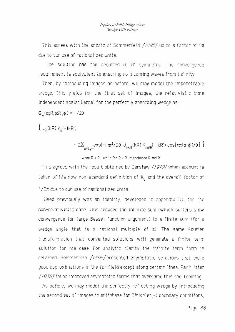
Topics in Path integration(Wedge Diffraction/

This agrees with the anzatz of Sommerfeld [1895] up to a factor of 2n

due to our use of rationalized units.

The solution has the required R, R' symmetry. The convergence

requirement is equivalent to ensuring no incoming waves from infinity.

Then, by introducing images as before, we may model the impenetrable

wedge. This yields for the first set of images, the re lativ istic time

independent scalar kernel for the perfectly absorbing wedge as:

Gw(a;R,*;R',0 - 1/20

{ J0(kR) K0(-ikR')

+ 'JZ exn[-inn3/2B] J r Jk R ) K J - ik R ’) c o s ( r m ( ) / 6 ) }n=i,i-a nS/t} na/o' '

when R < R.'; while for P. > P i interchange R and R’

This agrees with the result obtained by Carslaw [1919] when account is

taken of his now non-standard definition of K and the overall factor of

W2n due to our use of rationalized units.

Used previously was an identity, developed in appendix 111, for the

non-reiativistic case. This reduced the infinite sum (which suffers slow

convergence for large Bessel function argument) to a finite sum (for a

wedge angle that is a rational multiple of it). The same Fourier

transformation that converted solutions w ill generate a finite term

solution for nis case. For analytic clarity the infinite term form is

retained. Sommerfeld [1896]presented asymptotic solutions that were

good approximations in the far field except along certain lines. Pauli later

[ !9 J 8 ] found improved asymptotic forms that overcame this shortcoming.

As before, we may model the perfectly reflecting wedge by introducing

the second set of images in antiphase for Dirichlet(-) boundary conditions,

P ci g e o h

Topics in Path iniepration(WedQe Diffraction)

or in phase for Neumann( + ) conditions. ! o yield:

& VJ ,0 ./ ~ 2/0

[ 2 exp[-injt2/ 2 0] j ft(kR) K sin(nn0/0 ) sin(nn078) }n-i

G.. +(O£;R,O;k ',0') = 1/0 1 Jn(kR) KJ-ikK*} +

2Z exp[-irnt2/20].J^8(kR) Kn„,a(-;kR') cos(njt$/e) cos(nn078! 1n = l,c-: yi/6

when k < f " , while for R -> R’ interchange R and R’

In agreement with the DirichletC-) result of MacDonald [Z902J


Remark

Throughout this analysis we nave continued to sum over all paths, and

have avoided the introduction of path constraints to implement boundary

conditions.

The use of a superposition of solenoids in fact replaced a constraint

condition (impenetrable surface) by a suitable use of potentials.

Pane 90

lo p ics in Hath integration(Wedge Diffraction}

Appendix I

Riemannian Sheeting

A multivalued function may be made single-valued by considering it to

live upon a many sheeted surface. This description is a substitute for the

use of branch cuts.

For example; the cube root of a complex number is trivalued and would

live upon a three sheeted Riemannian surface. These sheets connect where

the branch cut once lay. Upon crossing this connection, transfer is made to

another sheet in the manner indicated In the figure below.

The use of Riemannian sheeting in making a multivalued function

single-valued

'his picture general ^ .m r z j j j p Sj v d y J : L i V d i U c U jnctions.

P330 9 •

Topics in Patti Integration (W e d g e D if f r a c tio n )

Riemannian sheeting is more than just an alternative to the use of branch

uts, m that it makes clear the distinction between positions on different

beets. ! his is an important feature in the use of such functions here.

Pace 9 2

Topics in Path integration(wedge Diffraction}

Appendix II

Solenoid Superpositions

Following the procedure of before, we choose to superpose combinations

of needle solenoids to achieve a free field kernel satisfying the desired

boundary conditions.

As discussed previously, our use of Images to Implement boundary

conditions leads us to consider a [i sheeted Rlernanrian surface. Only

solenoids whose strength (a) are a multiple of i/|x exist upon such a

surface. 5o choose combinations of these solutions such that the source

lies Within tne physical sheet.

Namely tnat:

L:mM0+K = S(R-R') 2 n= Mt5((o-0'} - 2iqtn;

Starting from the arbitrary linear combination:

K = p/ijit exn[ip(R2+R‘2)/T] 2 a ^ J (2R‘Rp/t)r '■ r ’ n= -«« n in/ul r

p/ljiT explip(R2i R'25/T] 2 a_ l rl (~i2R'Rp/t)n=-eo,*i •=

but Tor \Z\— ? ° ° :I (z) -* ez/V (2nz)v

!arg z! < n/2(regularization is implicitly used throughout)

t-*Q+K =

Pace 93

Topics in Path iniegratioi(Wedoe Diffraction)

Ling pi ini exp[ip(R2+R‘2)/t] T in/4nR‘Rp) e 52RRp/t 2 a_ e in{#'■-*u‘r n=-«}« :i

i he anquiar factor:

2 a V|if l = - c o ,co

is required to be a series of delta functions lying at 0-<j>’=2n|L x integer, ihe

a 's are in fact nothina but the Fourier coefficients of a Fourier series forn

s u c h a periodic deita function. rourier analysis yields the Poisson suni;

2 e!mQ = kin 2 5(6+2jin)n--co;to n-~c- co

f >-i i Ui n which one can deduce that the an‘s are in fact equal (a); and this ha?r!c

r y

iru^^K = Lim,_.0+ apt /(p/iJiR ’Rt) exp[ip(R-R')2/t] 2n=-w

5((<HO - 2flpm)

Limt_^+J 0 .. w (p/iiTH’RT) exp[ip( R-R‘ )2/t] R dR

The integrand contributes only around R=R'

= v (p/ijn){_ exp[ip(R-R‘)2/t] dR

;.e. the integrand = 5CR-R*;

hen;' c

■“ 11' 'x—fQf K = 3(1 S(R-R’) 2 5 (« H '> - 2Jt(l.n)

.e. a = 1 /ft

leiuiny tiiO complete K.ei nei or befoi e, hdineiy:

Race 94


K = p/ijn|i exp[ipCR2+R'2)/T] 2 e ^ (-i)W- j .(2R’Rp/t)

om wmcn W8 proc-80G as previously.

pa to

Topic.? in Path integration ■!edQ S D iff ra c tio n }

Appendix III

Finite sum expressions

To evaluate a finite sum form for:

S(z,$) = 1/2 J fl(z) + 2 ^ e“in* ,2p J n/ (z) cos(n0/|i5

where j.i is a positive integer.

The approach taken is to develop a finite term partial differential

equation (w.r.t. z) satisfied by 5, which Is then integrated to yield an

Integral form for 5.

Look at:

C / -r >, \ _ ! / •-

havlnn used:

-1/2 Jj(z) +

1 Jn v L / * 2 e"inR/:0 n=i,«

5 = ‘1/2 (F> + 5 ) $ -$■

2 e-in.il/2p | /2 ( ,n~l,

1./? (, ! - J 1'■***’" ~v—1 v+1

p-lnjiGp i aino/pe wn/|i “

(n/pv-i' (n/p)+l

n

(7\'\ a ' W P

andj t

■Q ~ "Ji

At ter considerable manipulation:

u u o' - i/2 e i»J0<z) - 1/2 2n=i,M

0ins/2{i j _ (2 ) gi(n-n)*/n

1/2 2 0-in*/2{i j fz) e-i<fi-n)4/|i _ j c o c a T p-in*/2|i i (7) pin*/pn=i,« R/p'

recan:

page 96


ds / dz = :/2 a(s. 3 J / a z♦

— _ ’ / ■ ) ~ a f —7 \ _ i / o "S'' 1~ grrnJm ? ■ —? \ _ ^ 'ns/2{i ; / —r \ T - { / j . _z~. ■ ~1/ i. e d z j v p 1/ i. I t ’ ‘ i../ b • *J . a ) J LUoyyji U/0/U.Ju n = i , | i - i 15'f*

- i coso2 e mnJ2 J , (z) cos(no/itn=l « n/i*

Lead<ng to the finite term partial differential equation for 5 :

a s(z ,0)/a z

■722n = t , M

which is of the form:

{ e'niW2t‘ J_n;ii(z5 - e~,nfy2!1 J n/jj(z) } cos((|t-n)$/|i) - i cos0 5!z,o;

a5 (z j)/az = p(z,0) b(z,0) + q(z,0)

~ j-\r< r> f hr. q r \ 1 < i +■ i r-\r \•cj! iu i lab uic bu iuuOii.

where f -ir"

upâp-

>(z,0) = exp[J p(z,0) dz] { qiu^) exp[-J p(.v,0) dv] du + f(o) }

an arbitrary function of 0.

5 (2,0) = e_izc05* { - i / 2 2n = i , } i - i

-mo/u

Q ,z ' -n/ji

r , ! :•»- -7 — A f i n H ft A > "r .K ’ i- ’ \ / Ci ~ f ( ip ’-i i- > i i iu i \V|}/. i i i I ■_> L j l V C O i } j ~ 1 i

hcivunu ub0Q the iaci tnat:

| 0 (u) - e-'™'21* J (u)] eiucos* du * ft$) }

J (0) = (S y>0V ■and

J0(°) - 1

rinaily tne identity is obtained as:

1 /2 J (z) + 2 e ,n*/2|i J n /(z) eos(n0/§i)

Page 97


= e iz cos* { - i / 2 2 c o s (( i i -n )A /ii}n = l , ? - l

f [ ein»/2? j {u ) _ g-iim/2* j (y )] eiu cos* dU + 1 /2 } J 03Z _n/P n/p

This reduces te the known result for |i=2 [Gradshteyn andRyzhip P973

f r n r n JR S' / / /’ S' l / n n rn p 1 v / •/ / u - v / / _ ■ / t I w * / y f i i u i i i C i ^ .

• /2 J J z ) + 2 e inRM J J z ) cos(nA/2)n=5 n/2

by using:

-i/2

= v C i /in) e 1Z cos*

(z) = 4{2inz) cos(z)and

- i ( 2 z ) cos(§/2)r • iexons-j d<

J , ( z ) = •/(2 /nz) sin(z)i/2

me euucKson:

1 / 7

and the variable chanae:

2 = -/(1 / Itt) I explis2! ds -> -»,o

b = / (2U ) C 0 s(§/2 )

One may fu rth e r generalize this identity by adding together

expression for angles given by:

d) + 2nk[i/v

where v i s a oositive integer

The left hand side of the identity developed becomes:

is — » ...V

\ / £ 4* l UnU,' T JL*K=1 ,V n=i

e-inft/2ji j ; (2) [ 0~in(-t-2Rk|i/vy{i + ein(+2nk|i/v)/|i ] ]s n.'ji

OUI:

— v if n is a muiLip.e of v

Topics in Path In top/ s i ion (Wedge D iffraction )

2 2akn/v

= 0 if not

This is most easily seen bv noticinq that this is the sum of evenly soared

unit vectors In the complex plane.

So the left hand side becomes:

1/2 J n(z) + 2 e J nv/p(z) cos(nv$/|Un-i,oo

= 1 / 2 v 2 { e lz cos(#+2ak^ v> { 2 c o s ((|i-n )($ + 2 jt k |i/v )/|i}k = i Jv n = l , | i - l

^[giiM p j n/a(u) - e"in,U2p J n/B(u)] eiu du + 1 } }

These results are useful in that they convert an infinite series which

suffers from slow convergence (for large Bessel function argument) into

an expression with a finite number of terms (for iiy finite).

Page 99

fop/os in H a th Integration ( W ed g e D if f r a c tio n )

Appendix IV

Decomposition of the electromagnetic waver ! -I ' ■ /«-■lacKson, / P 75/

inside a perfect conductor, the electric and magnetic fields are zero.

Using Maxwell's equations to see what this implies just outside of the

surface.V.B = 0 SI E = -dB/dt

OdUbh •I> lUKOS

<j>E.di = -a/at je .d sfB.dS = 04 i

iihi: loop integral 5 y rr! 0 o 11 z i n g the u e oi d ciosed sun ace ) + 4

(B L = 0n 'r> (E,>s = °n: norma! t: tangent

Sim ilar deductions cannot be made from the remaining equations, since

the current and charge densities are infinite on the surface.

A more convenient form of the first condition is obtained from Maxwell's

equation for free space.

V 5 = i / c2 aE/at

(V 5), = 0

Yielding two alternative, independent boundary conditions:

L 0

Paqe i 00

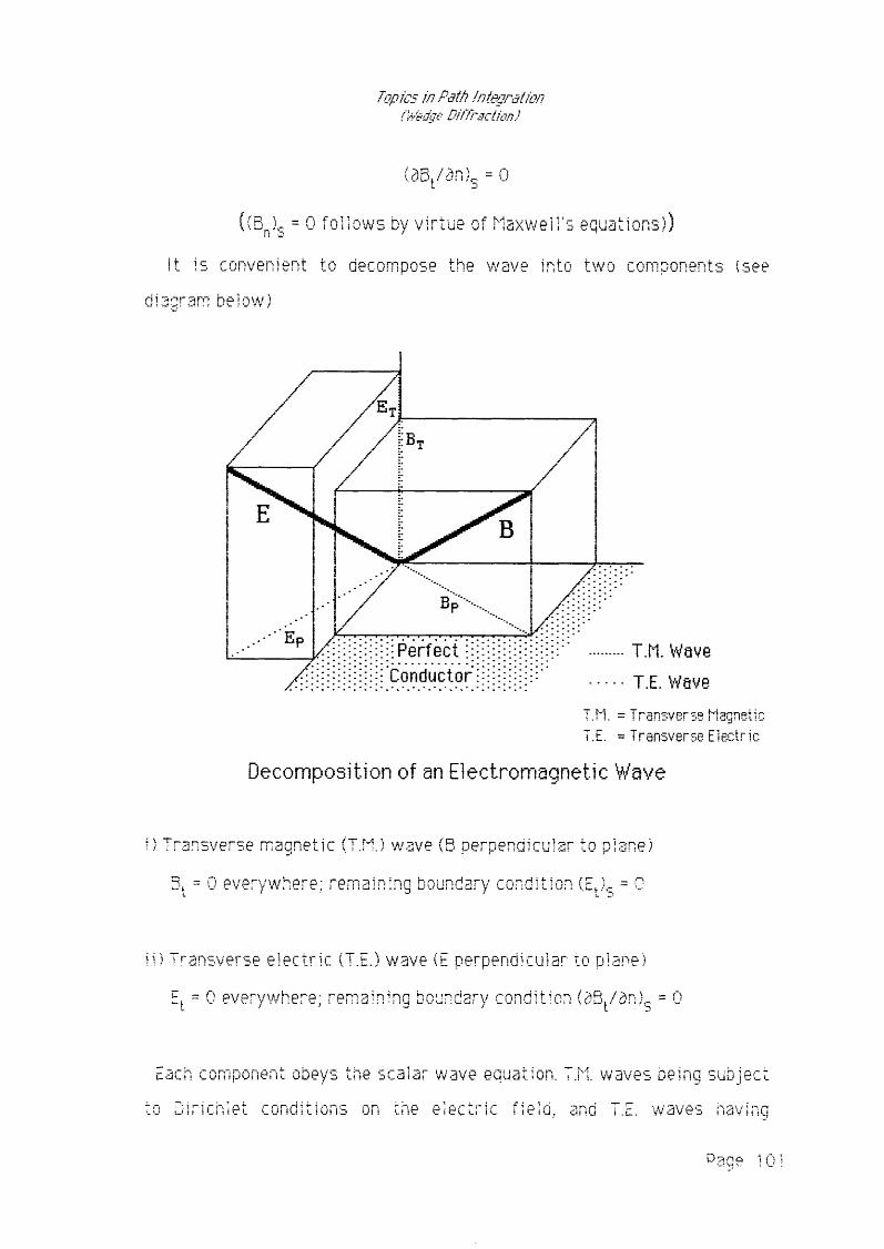
Topics in Path integration(Wedge Diffract inn)

O B ./a n ). = 0t 3

((B JS = 0 follows by virtue of Maxwell’s equations))

it is convenient to decompose the wave into two components (see

diagram below)

Decomposition of an Electromagnetic Wave

i) Transverse magnetic (T.M.) wave (5 perpendicular to plane)

3t = 0 everywhere; remaining boundary condition CEJS = 0

11) i ransverse electric (T.L) wave (t perpendicular to plane)

Ef = 0 everywhere; remaining boundary condition (d5t/dn}q = 0

Each component obeys the scalar wave equation. 7.M. waves being subject

to Dlrichlet conditions on the electric field, and T.E. waves having

Dgno 1Q

Topics in Pstn integration(Wedqe Diffraction)

Neumann conditions on the magnetic field. (Tf boundary conditions

Induce ref looted waves).

Paqe 10:

Topics in Pain fniscjrat ion(Canonical Transformations J

Cknpler Tk ree

ca n o m c c L ' / T r a n s fo r m a tio n s

in

(Q u a n tu m f \ e c f ite c n a n i c s

ononicaily invariant discretization Drescriotion tor the oath in ' i i I i

Topics in Path integration(Canonic-?! Transforms Hons)

SI Introduction

in this preliminary work canonical transformations for the path integral

are identified to be those of classical mechanics, and a time

discretization scheme found that allows the transformation to a trivial

Hamiltonian, as well as a consistent quantization of a classical system.

Traditional quantization through operators [Dime, 1958; Chernoff, !98F

does not generate a unique quantum theory. Equivalent classical systems

(related by a canonical transformation) in general yield differing quantum

systems [Kapoor, J984J Also, in the operator formalism, it is not clear

how to implement a canonical transformation due to the use of

non-commuting variables. The ambiguities in quantizing the classical

theory means that one cannot fall back on the classical theory to perform

the canonical transformation. The path integral description of quantum

mechanics [Feynman, 1948; Feynman and Hihbs, 1965] offers an

alternative method of quantization and poses a possible way out of this

dilemma, since it uses commuting variables in its structure.

Starting from the classical action, one can form the path integral

expression:

J [ el7T) /<*r hmi Dq Dp

This formal expression is deceptive in that it employs commuting

variables, but is supposed to oe equivalent to the traditional operator

formalism. The above formal expression is in fact ill oefined. in order ro

evaluate it one can discretize it in time; but the answer is in fact

dependent upon the finite difference scheme adopted. Factor ordering is

carried within tne prescription [Schufman, /980;Mayes andDowker, 1972/

Page 10

Topics in Path integration{Canonical Trans formationsJ

!n general, however, the prescription w ill change under a canonical

transformation [Kiauder, 19801 so a quantization scheme based on a

particular prescription w ill In general generate Inegulvalent quantum

systems from equivalent classical ones. These features have been dealt

with In more detail in the introduction. However, a particular

discretization scheme has been found that is invariant under General

canonical transformations, and opens the way to a consistent quantization

scheme, as well as a quantum mechanical application of the

Hamllton-Jacobl theory of classical mechanics [Goldstein, iQ8Qt

5ciiu/man, 19801

Pace 105

Topics in Path integration(Canonical Transformations)

II Canonical Transformations in the Path Integral

In classical mechanics a canonical transformation Is one that preserves

the least action principle [Goldstein, 19801 For the path integral one

might analogously require that there be a path integral representation in

the new variables (Q,P,t), If one existed In the old ones (q,p,t). Such a

transformation should be system independents that Is to say, the

transformation should be canonical not only for some specific system, but

tor all problems with the same degrees of freedom. The amplitude may

alter under such a transformation by at most a phase factor.

l.e. form ally, with end points (a,h) in phase space held fixed:

j J e:/* i!pq - H J d l D q Dp _ gi/fi (Ffe - F.) JJ g i / T , I f P Q - K W t p,q D p v H(qjPjli

F being an arbitrary smooth function. Assuming that a canonically

invariant discretization prescription exists (just such a scheme being

sought), then this formal statement becomes true for that scheme. Any

other expression should be manipulated into this form with the resulting

O(tr) term additions to the Hamiltonian. These terms may be replaced by

'potential like' terms of the same effect [McLaughlin andSchu/man, L976L

the technique for achieving this being illustrated later, it Is being claimed

that the quantum canonical transformation Is a cleaner object when used

with an Invariant path Integral scheme.

Since the above equation Is to be true for all Hamiltonians, the

Integrands must be equal. This Is perhaps most easily seen by choosing

Hamiltonians that are highly localized In phase space. The Integrands must

then be equal at the 'localization point'. By choosing Hamiltonians

localized at each point, it follows that the Integrands must be equal

Page 10

Topics in Path Integration(Canonica! Transformations)

everywhere. This imp]les that:

pq - H = PQ - K + dF/dt

if the end points in phase space are fixed, i.e. we should work with a

coherent state type path integral [Klauder, 1980] This is the same

requirement as in classical mechanics [Goldstein, 1980]; as well as the

further condition that the Jacobian of the transformation be unity.

Supoose F = F(q,a,t); then because:

pq - H = PQ - K + CaF/dq)Qtq + (aF/0Q)qiQ - ( a F / a t )qQ

and by the Independence of q and Q:

p = (a F /a q )Qt p = -(a F/aQ )ql k = h * <aF/at)qQ

F being now seen to be the generating function of the canonical

transformation. It follows automatically that the Jacobian Is unity

[Goldstein, i960] One concludes from this that the quantum canonical

transformations are the same as those for classical mechanics, excepting

that scaling transformations are excluded.

If one could perform general canonical transformations in quantum

mechanics, then one might consider emulating the Hamllton-Jacobl

Philosophy of classical mechanics. In this approach [Goldstein, 1980,

Schulman 1980] rather than directly solve the equations of motion

following from a given Hamiltonian HCq,p,t), a canonical transformation Is

Implemented that renders the transformed Hamiltonian (KamiItonian

K;q,p,u ) equal to zero. The work then lies in finding this transformation.

the generator of which Is determined by the Hamllton-Jacobl equation. r or

this purpose it is convenient to work with an alternative generating

function given by:

F ( q ,P ,U = r (q ,Q ,L ) + GP

Paqe 107

Topics in Path integration(Canonical Trane formations)

pq - H = PQ - K * dF/dt

= -QP - K + CbFi'dq)ni Q + (bF/'dP) , P * VdFFbt) ,ri. Ql Qr

from which follows, by the independence of q and P:

Q = (dF/b?) , D = {dF/bqU K = H + <dF/dt) nql ' Ft 'QK

leading to the Hami iton-Jacobi equation:

H(q,fo/73q)pi>t) + (d/7£t)qp = 0

Classically one has transformed Into a frame that “tracks1 the system

mat ii then has trivial motion (constant phase space coordinates),

transformation then carries the motion (see fiqure below):

a

The Hamilton-Jacobi transformation

Topics in ro w integration(Canonical Transformations)

Sill The Symmetric Path Integral

Due to the higher order sensitiv ities of the path integral [SchuJman,

19801 in order to correctly transform the path integral one can start from

some time discretized version. An especially convenient scheme for the

Dropagator is the 'symmetric' prescription given by:

Kfn. n. t. In n t ; =t 1 : \ • i t :

i l l ........... (dqtj)dp (.j/2n.n) j = i ,i — ! tl!expjj/ n 2 pr,(k)(Q(k)~Q(k-U) " H(q Ck} (k),k-l/2 )At }]

wnere:q tk) s i/2 (qfk) + q(k-n)

pm(k) = 1/2 (P(k) + p(k—!))

At = T/N

The end points not being integrated over, allowing them to be held

constant. This is most closely related to the coherent state path Integra]

[Kiauder, I960] where end points are naturally not intearated over and

there are an equal number of coordinate and conjugate momenta

integrations. In general a given phase space path Integral (with fixed end

Dolnts) must be kneaded into this form with the cor respond inc ft2

additions to the Hamiltonian, which Is then high

nature. What has been achieved is an 'exposure* of

use of the symmetric (mid-point) f inite deference expressions was

then hinhiv fllian.fijrn p-pfhanjra’ 1 P

posure* of a 1 stochastic terms. 7• 1 P

■snrjUl !U motlvated In the Introduction to path Integrals. 5y

n f" — r*; • i u 3 C i nJ immy van able., this rnid-poirit ordering can be seen to

to ‘Wev1 ordering' i n the ooerator formalism [G-crvafs anc

’aoe ! )U

Topics in Path Integration‘'Canonical Transformations)

Jevicki, 19801 The properties of mid-point investigated earlier suggest

that the proposed discretization might he the canonical invariant sought.

The end conditions are not always independent, since if one wishes to

recover the classical limit as tv+0 , the end points must then be connected

by a classical path. Any two end conditions are then sufficient to

determine the other two.

There are in /act pa irs o f points in configuration space that cannot rejo ined by a least action principle, for any Hamiltonian [ L andau andL ifsh itz, 1982] Motions between

such points would not have an 'action d escrip tio n It is assumed that coordinate systemsleading to th is dilemma are not adopted.

This manner of path integral has been investigated by Kiauder [1980] dnd

would seem to be the starting point for making the path Integral a well

defined mathematical object [Daubach fes and A Jauder, / 985j.

Pane ’ j 0

Topics in Path integration(Cjnoo/cj/ Trj/isthrewis’ons)

SIV Transforming the Path Integral

Consider a general canonical transformation of the p and q implemented

by a generating function F(q;o.,t).

r\ — t A l- / n 'H - yul" / uU.inv' UU.

P = -OF /d(j)ri K = H + OF/Ot),T5- ■

(could use any other generating function)

or ecuivalently:

q = qCQ.P.t) U = Q(.q,p,t)

p = p(Q,P,t) P = Ptq.D.t)

r i i p f\ r •“ +i • US ;Ci U

oo/aq) t =• "i n t Op/5P)Qt (an/dp)qt = -(dq/ap -Q t

O P /a o ) : =• p t-(dp/dQ)pt (aP./dp}qt = Oa/dQ)Pt

it is useful to first consider the formal canonical transformation of the

path integral with no consideration of stochastic terms.

Formally, with all end points fixec:

j j pi/n j(pq - H)dt Qq Qp pi/n (F - F,) JJ pi/h J(PQ - K)di qq pp

K(0.,P,i) - H(qJp,t) + (aF/cIt).^

so that using the symmetric expansion scheme this is interpreted as:

0;/n i-b- pj iim }. |II (duej)dPc,(j>/2nn)I'i— y J j=j M- } i'i

exPli/ n , \ P * k) \ ?■.)_ U:( k~ • I } ~ K(UM(k ) ,r;."l/2 j Al /j

KiO^.Uk} i ,k-i/2 i - (k) ,P^(k) ,k~i/2 i k U r / 0 1 1 q

D. (i-'i - ’ /■-. + Dr.-- s, \ ''-W---- • - ■ / i \'-aV'-- ; ! / •-

Page !

T o p ic s in n o th in te a r a l l o n

(C o n o n ic a ! T r a n s f o r m a tio n s )

D n-'i = ’ i n ' D i i - 4- \i i

qtXk) = Q(Q ik),P ik),k-i/2 ) pMCk) = p(QMCk),PM(k)Jk-i/2)

Under this notation an m subscript means at the q,p mid-point, while an M

subscriot means at the Q,P mid-point.

in generai the naivery transformed expression is not equal to u s parent,

oue to the Generation ot extra (stocnastic) terms m the process, inat is to

say, a general discretization prescription is not canonically invariant

[Kfauder, 1980] The task ahead is to correctly perform a canonical

transformation and determine the stochastic terms so generated in the

hope that they sum to zero, as required of a canonically invariant scheme.

x

Topics in Path integral ion{ l rnozi/cj/ Trora? formations )

SV mid-point Expansions

or use are mid-point expansions, since in the symmetric pres*

functions are evaluated at the mid-point.

Adopting the following notation:/ m U ) = / ( q m(k ) ,p mCk},K-i/2 )

/M (k) = f{ q(G<..* (k i,Psi(k),k-1/2)7p(0. (k),P N> (k),t—i/2)3k-i/2 )

/,Q = (dF/3G)pi /,p E OF/dP)Qt /,t = (dF/dt)0P

7 nn

Af(k) S f(q(k},p(k.5,k) - f(q(k-l),p(k-! ),k-1)

Note that this implies tnat:

Q (k) = 1/2 (q(k) + qck-n) UM(k) e 1/2 (Q(k) Q(k-1))\uKq-qtc qMik) = qiQm it ,>7-1/2)

sim ilarly for p, P.

Then by Taylor expansion:

+ 1 /R f" " J >1J0U AQ AQ

♦ 1/5 fW P' : ! • AP AP

+ 1 /'r\ fI M ’ll At At

<-•

f5-u AQ AP

l/ /r-UQ f AG At

- 1/4 jw.T•f !'! ■ •_ AP At

A/+ f P,/ M ••

f M,»" M • Li/24 f~,r,r,n v 1 I' uuU

AO

AP

At

Au AO. AU

l> ~i n p

+

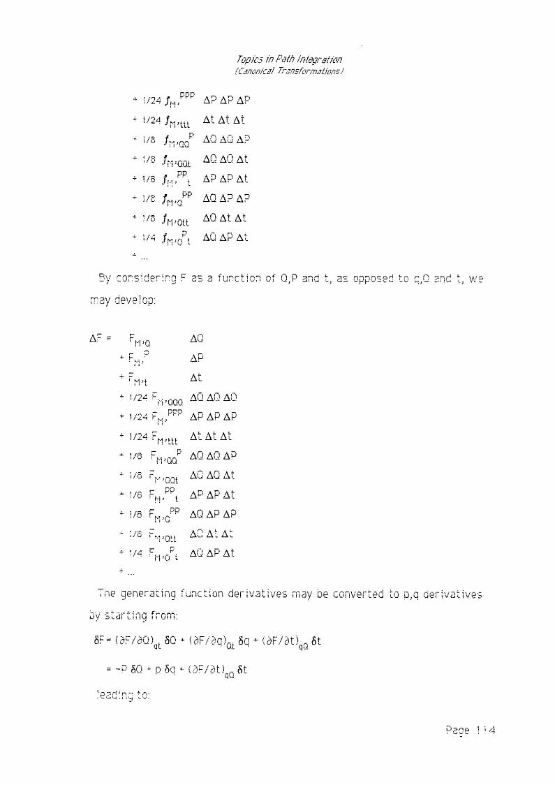
Topics in Hath integration(Canonical Transformations)

**~~vTC-l PPP

j AP AP AP

1 /2 l / r 'tit At At At

1/8 /nP

JQQ AQ AQ AP

1/8 JM■QQL AQ AQ At

1 /o / mPP . 1 AP AP At

I/O / mPP

’Q.AQ AP AP

!/S •Qtt AQ At At

1 / 4 P*Q [ AQ AP At

5y considering F as a function of Q,P and t, as opposed to c,Q and t, we

ay develop:

AF = M JQ AQ

AP

At

+ 1/8

+ 1/S

1/4 F

rPQGQ AQ AQ AQDDD

rrV ' ’ AP AP AP

rrrttt At At Atr— nu_ r* M |AA AQ AQ AP

' !Q()i AQ AQ Atc PP•! fvjl t AP AP Atr- DUr rW ‘ AQ AP AP

AG At AtU ¥: rl'Q t AQ AP At

i lie qenei a>_is\q s ui\l ■_>un Gei ivaliveb ■ iiay o0 l0nv01 •.0g >_o d,q got1val 1 v

Oy a •_arf ] nq i rorn:

Sf = (dF/dQ) : SU + (dF/dqL, So + (dF/dt) Stqt Qt qO

~H Su + D 5g + (dF/dt) St : * qu

1 p r- H - n n. ~ n ■ - •1 'H

ppr;p 1 i yj.

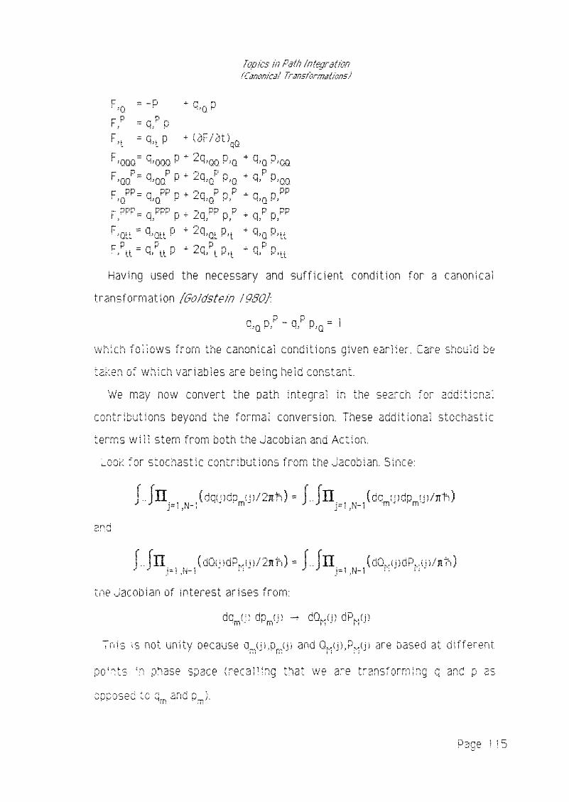
Topics in Faff? integration(Canonical Transformations)

' 50. r- Pr ;F,t

F.,

M«~ M; U

= q,t P

= rQQQ H;OQQ p

r,QQr = ^ n P p +p p p = a' -’Q h ,Q

\j \/,r-:n KK r\

PPP r.M? P

•a

i a F / a t )n0

’I n n‘_ L|iQQ ‘ ;Q

P! Q2 a ,« p d p‘•u. 1 J2q.,PP P p 2 q?QL p,tWqw PjQtt ';J

p[\i = q,%t P ■" 2q,ht p,t

” Q , P

q,q;Q

q,p

-QQP-’QQ

nnP,rr

DDP,'

Pmnr-‘ i

Having used the necessary and sufficient condition for a canonical

transformation [Goldstein iQ80[

n n *■' - n p D = IN M: r ?Q 1

which follows from the canonical conditions given earlier. Care should be

taken of which variables are being held constant.

We may now convert the path integral in the search for additional

contributions beyond the formal conversion. These additional stochastic

terms w ill stem from both the Jacobian and Action.

Look for stochastic contributions from the Jacobian. Since:

j . I n (dqC0tiDm{j)/2rh) = I .. f l l (dqjudp in/nti)j j j_; 1 mJ a ■> i=1 N-1 m - 1 m

[ . . { n . . t _(dQij)dPM(j)/JlTn) = f l l (dQmodPmn/nn)J j=? ,N-i - " ‘j=! ,N-I

tne Jacobian of interest arises from:

do n: do u) dQ,ji) dP.,(j)

Tnis is not unity because qwjhPPJjj 2nd Q^tj),PM(j) are based at different

newts w phase space (recalling that we are transforming q and p as

n n a a c fi d * a , ■"* 3 n d n ’jj C b v. \j (_ii i\_i p / .

Topics in hath in tegrsi ion(Canonical Transformations/

Jacobian:

J = (an /hi) ) (an /aP ' - fan /aP , fan /an )_• - -im' " ~M /p» - r- rri' ! M-fif ' - -im' P M T4 ‘ Hm M Um - ! M'Gt ‘M 'Pt

\*J ! *! ] {~ Pj ! R C

q,,, pN, ,r‘ - c

4- i /e f n

n r n■-i j M m > >

i,u ^M'QQQ HM* HM'QHrVQQ P,M , Q 'M' ~:M;Q ^vj PPP

4- ;/R H P - P +

+ Ml

n • [ !"mpQQ P1 \ . _ . j ,• '•iVjisit . Mj-’Out ' M

■ i/ o \ q f pt-.-’ j

Qm-’QPm,■ tt - q,

qnJQPn, .PP - n,■y -•]nmmo

n*j. P _ r.■Q i

—rrj

D

x n r, PP ' t

Mm, Pj-v QQLr)

nMrl

p’QO Pn, n iv.< AG AQ

qM.r-’ r r} a'M \

JQ' AP AP

q{13. H Pm if)* I u At At

qM PP■’Q Pm AU AP

n PMKi ,rv ♦! i U. l- * j {•\'if AQ At

qnDDf ’ t

r\Ut.4 .‘ : !'■fy AP At

but, for a canonical transformation:

n n p - n p n = 1M,q Ki M, »-mq

Bv aoDlvina this at the M mid-Doint yields:

, j = I + i /4 (ri P n - n n p") 1 ,/M VL*M'G A im s S'i-*QQ • MJQ ^

.i. ' / a ■: n Dp\ / ‘ KM'Q+ i (n r n: / : \ Mm j r-

r«n

r-j on xqM ,Qr Pr-1- ■ >n n‘i-i > L :VQl Mj--] > Qi. Ph , v -'

— M* U* ^* i/8 i.q..., ,■ cv,■ Mi > ' r-. J I -i

/-% r-

' r i- 1

»**. * , r\i i ' '11 ,r,r, Km1 l

JCQ +nMM

D•’0 Km>QL mm jqq

- P km > t Mj

i P + M }0.

nhm

r p r>, Pn O' « r, PhfUQ n” p.L'l.3 , f* n3 L - n,“i

AQ AQ

AP AP

At At

AQ AP

mm \M-’Qt • M-

Lontinue bv iookino at the Action term d (m AG(k> and cornoanno it*■ - rn

P*.,(k) AQck} + a F(k) - (dFM(k) / d t ) ,n A t ; its formal counterpart.

pm Aq = AF < P„ AQ - (aF „/3 t)„n Atn' "‘iM .'Q ; M -(Ji) ~r1 ;00 * M; Q1

q QAQ AO b

Pace

Topics in Path integration(Canonic*/ Trans formal ions)

rr _

1/24

1/4

1/8

I / 8

i /4

(r Pn DD x hm > ;-?4 >(q„ n,,* + r MI i LkL * i

( n n f\ Hm >n Hm in: ! 'J. i 1 >_».

! n

f"' n' I f

kPfpQ ^M’tt + ^M ji Pri;Qt (n p n + '?n n p - a p' -if.-j > K M j f f ^- -iM J j K m i -ir-j l H

PP „ Q.. h n.iM ? n r

Q m J t P m , J. 4. F m 3 j. i. i< i L 1 I t . k I I a - LL

M m ,!- fs

■ \ M m , n ■

o o D,..* j“j x a , , Dm rUi • h ’QQ4- nr -Mri.Q Pf- J 0 1

KKf Pm + n n ■M -’t • M

PP+ 2 m-’

nr D.' ip■’ I

P r\ + n n P . _ p *+ ( • n +o t kmm mm•Q !"M-

Fn'PP

m

P - q P n i mmo Lnjn" )

+ MMjfV ' Mm inti Pf n-'M M > H

AP AP AP

At At At

AQ AQ AP

AO AQ At

AP AP At

'n, f L) AQ AP At

AO AP AP

AO At Al

AP At At

Finally, determining stochastic contributions from the Hamiltonian. By

again applying the canonical transformation at the M mid-point:

K m = Hm * W f./ d t ) qQ

.he oriqina; Hamiltonian becomes:

K« - (3Fn / a t V4.

1 / 6 H,•|JQQ i> O AQ4- I/O H,

nn -* j AP AP

4- 1/S H‘ s' - tt At At

4- 1/4 Kip

•no. AQ AP4- 1/4 H.iI ’Qt AQ At4- :/4 Hr■v i AP At

)Q up tne stochastic terms:

1/4 Di n *■ n nhim -mw“V“\• uU Mm . “v i ( ‘, t , m Dpn p n Pi / *-t pri m Mm :-n

+ 1/4 in P n r*• -hi; t f-'M ■ n PP r

mt '-huot+ i/u Mvi Pmmo" l-M 3QQ

' n p 4- p\ i U‘ *-i w\ * t »-• K'lCl' * Itj {-\ n% M[-MQ

D\’Q } PP>i

(0PP\

- n n r. - n ?-f}+ -!M >HQ KM ? f -!M ■’r"M mmjQP-.

AQ AO

AP AP

At At JacQhiai AQ AP contribui AQ At

Pace

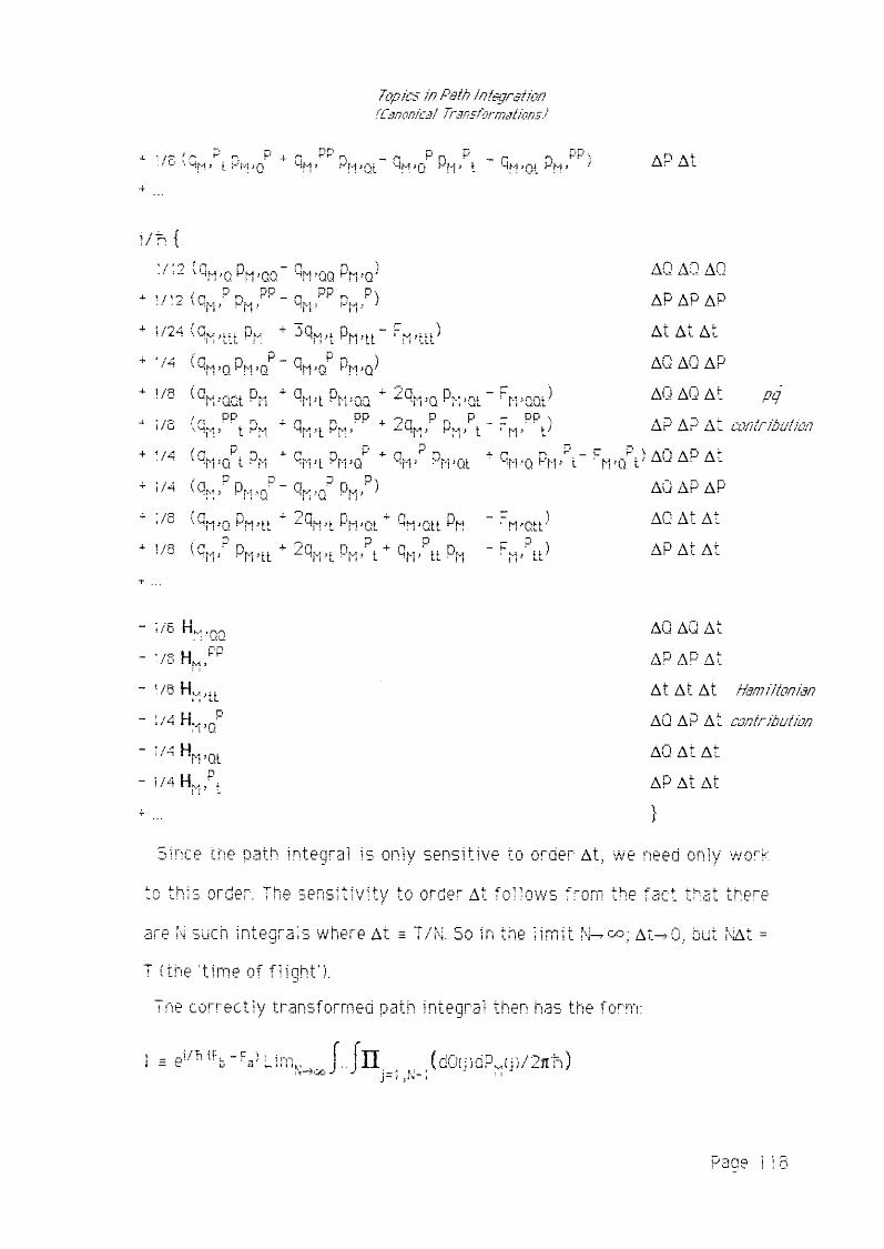
Topics in Pstn inieproHon(Canonic*! Transformationsi

r-, n rs r-. n n n+ ; /F; ' Q r , r, h + n rr n - n p n - n r> Kh‘ ’ ~ •Jj-'j > f- M -If--1 ; Q r~ f--] .■> r HM »nf •‘“‘M* AP At

1/ h t

:/;2 (Hm ■’0 M;-i jQQ 4nijqq Pm-’Qn n n4. t /**—»«' r \ •*“ r\ r r — < ~ r \: / : Z \ l|M , Mm , '-[--A , Mm , J1 I • ' ! M ‘M ' <r

+ ’ /•-) .-= / n n 1 7 n n _ ET ^! / . ‘1 j (.14 Mv M-jVijj. rhilM 1 M U ' i LLL ‘ . ! I •_ ! ! i.L : I LLL

T /*i

+ 1/8

i/u

+ UA

+ ]/4

- ;/s

n n p - n t r n i - H ’fi m m jo

p p! S”' M ,Q

Q m . ^ P m + a M j ,i 1 ' VjiO«.L i i I I InK n !Q u

,.T p p4 m j [ H n

4- m n PPM m ,

p -'•Q 1. . i }«j t, jt C U r- * r

+ ri T n t

n PH n JQ

Q n ~ i _ D

/ fi n J--M-1 ’f; !“V' > )MJQ *“M3Qi ' h'GQt'

D D - D P4- ,-!n ‘ n h - - ■ ■ ;■h - h m j t * n-’ t-

AQ AO AQ

AP AP AP

At At At

AQ AQ AP

AQ AQ At PQ

AP AP At contribution

UW Pm.W - qm,.-“ dm ; )• ■ i i • u ‘i ; • u 'f r{n p 4. 7n n -f •-i n•■Mj-jjQ Kj'-jjfK Mf-?

D P 0< n * n + v n n • + n n\'KMj i-'M lii ■i-MSv! ti M m t i- M M 1 U U yU • i ! • t l i! - L • ! >' >- I ! • Li. • ! I

%>Q P i C r A -o V AQ AP AtAQ AP AP

'i• rpQtt AQ At At

AP At At

! / U H - , ,~v

- :/S H,„r'- 1 / 8 H. ..

« t L L

- 1/4 H „ >QP

n M5Qt

- i /4 H» 0 in *

AU AQ A t

AP AP At

At At At Hamiltonian

AQ AP At contribution

AQ At At

AP At At

Since the path integral is only sensitive to order At, we need only wor k

to th is order. The se n s it iv ity to order At fo llow s from the fact that there

a! c iN such integrals where At = i / m. mu in the iirn ii i\—too; A t—r j , out a At ~

T (the Tim e of f lig h t1).

The co rrectly transformed path integral then has the for m:

I = cs’/Tl l f u - F , J : im f i 1 1 f m u / D-wp-Ai — u a »— 1 I 1 _ j .. j XJL \ » vt * / / -i.il i 1 /

H3Q0 j • d

Topics in raifi in (opr at ion(Cunonicsi Trsnsfomstions J

I I ( I + -jacobian stochastic ter mb)k= i ,N

exp[i/n{pM(k)(Q(y-Q(k-‘ }} - K ( t k ),pm(.k},k-1/2) A t + Action stochastic terms}]

Now work to replace the stochastic terms by a potential like term

[ n c L a u q h Z f n a n d S c h u / m a n , ! 9 7 6 ]

ViQjv; ) At

of the same e ffect (to order At).

5o further define:

o = e 1 a l_ 1 mt f.. fn ( GU(j )UK,( I)/ zJTn)•WQoJ J j=1 ,N~1 ri

expti/1h (k)(Qck)-Q(k-1;) + K(%ak),PM(kU-i/2 ) At + V(On&)) At }]: j-.'l

Working to order At:

I . . I I I (dQ(j}dPM(j}/2nih)b r ai ,L im ,N—±<xs

11 (1 * Jacobian stochastic »_ei rns + )/ n Action stocnastic tei ins*k= 1 ,N

expEi/ti { Pt1ik!(Q!ki-Qtt-:)S * K C a ^ u ^ u .k -K ) A t }]

,rin.i

j _ .-’/n (F-_ - F } r r~ ! I I I f C ‘- ' i H !D t : \ / ^fT Iit-$GQ * J i= * ] 1 jj 1 • *' 1

n (1 + M n ViQh-Ak)) At } w=i n •1

exp[i/ n \ KMik)kU(kJ U(k- 1); + K ( 0..(k),P (k 5,k - 1 1 2 ) AL / j

er now the particular

Page 1 19


'OP- r\ r* n o n t i a »Ol ! i iCi i_ 1 Uf

point canonical transformation.

Paqe

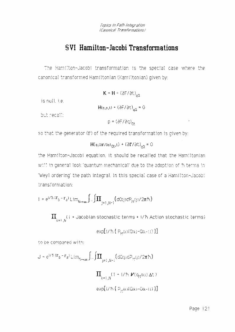
Topics in Hath integration(Canonical Transformations)

SVI Hamilton-Jacobi Transformations

; he Harnr.ton-Jacohi transformation is the special case where the

canonical transformed Hamiltonian (Hamiltonian) given by:

K = H (dF/dt)~' qQis null. i.e.

so that the generator (r) of the required transformation is given by:

H(q,(dr/3q)Qtjt) + ( 0 r / 0 t ) nQ = 0

the Harnilton-Jacobi equation, it should be recalled that the Hamiltonian

w ill in general look ‘quantum mechanical’ due to the adoption of m terms In

'Weyl ordering' the path integral, in this special case of a Hamilton-Jacobi

transformation:

n ( I + Jacobian stochastic terms + 1/n Action stochastic terms)

Hiq.p.u + (<3F/dt) q - U

p = (dF/aq)n,

k=» ,N

exp[l/n { Pr u;(Qo.}-Gu..-n)}]

10 be compared with:

exp[l/1h { PM(k)(G(k)—0(k-i)) }]

Topics in Path integration(Csnonics! Tr^ns/brmjtionsJ

The Toss' of At with the Kamiltonlan is ultimately responsible for the

null contribution from stochastic terms.

These integrals are ill defined and may be made tractable by the

inclusion of a 'mass’ ierm:

i nrN,A- ei/Tl ‘rb ' ra :nti)

n (1 + Jacobian stochastic terms + i/ts Action stochastic terms)k=i,N '

exp[l/1h { PM(k){Q(k)”Q(k-1)) + P^Cfc) A t/2 A }]

J = UrnM - r i/Mrb' ra!f - ] n f t ,(dQ(j)dP,,fj)/27tA)

I I ( i + 1/h K(&Ak}) At )k= 1 ,N !!

9Xp[i/h { PM(k)(Q(k)-Q(k-i}) p PM2(k) A t/2A }]

where the stochastic terms are:

: / ^ ^ ; v G ' - f U G G -’ Q G ! Q } AQ AQ

* /A (p PP n P - r. P n PP’', 1 m m j w-vo. Hn?Q K r i j ■'

AP AP

t Pf-i -’ot ” ^not Pm1 At At Jacobian

l / o ^M m T H P;1 30Q ~ ^rvQQPi' ■ AO AP contribution

: / c T h ; i P m ô q + Aim'* Pri'Qt’" 'Anaopnj t — n n P'5 4!WOt P M ' Q '

<o<

! / 3 % A w - r G ? + °iv?P ? n > G L - % > < ? » r A- q n P P ' iA-rot m - n "

AP At

1/ n i:/■ r-no rvQQ wrooPf-rcr

D D D D D D ,i/12 \Q.-.:, Pm / - q r,T ' >

’JlH Mri " 3CVni Print ” r rnttt;

AQ AO AQ

AP AP AP

At At At

Topics in Path integration(Canonical IronsformationsJ

+ 1 / 4

1/6

- ;/s

+ 1/4+ 114

+ !/S

+ 1/3

(qf1 n p ->Q ‘-Ir-ljri Pm.m; AQ AQ AP

C ,1 k nmat Hu W-nt M-QQ + zqM-'GPrVQt 'w , mot' AQ AQ At PQ

(q-! :

pD■" t Pn Q D ^ + Hn,t 2V n P -Km . t ■r n

pp \> H AP AP At contribution

% ■cTt P|-1 cM-’t ?nmp +i V PMmi + wi n Pm w-n t- r n,apt)AG APAt(q. D n

■’ Pfl'Q W Pf,. p) AQ AP AP

4 h■’Q Mrntt +4QM,t p ,.’Qt T Himu Pfl ■• r„ .JQLH AQ At At

Wnr n -*■ ■' yM'tt Gr-nt dm-■V n P"•rw tt p« ■■ c ’ Lt' AP At At

|/B M'QQ AG AQ At

- 1/8 Hm,PP AP AP At

- 1/8 H..,. At At At Hamiltonian

- '•« H.,...;' AQ AP At contribution

nr1,Ql AQ At At

- i/4 H , ; t AP At At

}

i n i s special case of a H a m ilto n -J a c o b i t r a n s fo rm a t io n K^0? so:

h - -Cdr/dt)qQ

= -r,t + p q,t

a s w a s sh o w n p rev ious ly .

T h i s lead s to the H am ilton s t o c h a s t ic t e rm s c a n ce l l in g m any of the ir p c

coun te rpa rts , s in ce the H am ilton s t o c h a s t ic contribution:

'n {1/

,/G (- r rijQQt + Mri,QQt pfi + -Vm.qi. Mm.q " 4k].|. j-V]»qq>' kC Ac Al

- :/8 ( - rM,W - aM ppt Pf, - 2qf1,?t PN,P * qt-.,t P„,pp! &P AP At

i/o + + zGrvtt Pmjt + ° -’t,/*- v-rM,Q-1 - »Q't Mri * q .Qt Mr.,, x qM,' t Pm<g * Pm-q' ; A;-*

- 1/4 ‘ q ,,Qtt D,. - q,,,QL P,.,. - q,.,,. p ,,Q - qK.t p,,,aj AO At At

- ',14 t - rr..,ptl * q„,ptl p„ * qn p. P;1,, * qn,u p,,,D * q,,,t d:, ,p,) AP At At

Page i2 a


}

1/4 ^M'cf pn'QQr n P \ •MJGQ • MJQ ' AQ AQ

+ i/4 (nM ppn., _p - • "‘f-1 * T'i’Up P n, PP

’0 Pf’1' AP AP4- , n> i A 1 p r n —

11 >- >1 \J£L qM,™ P , / ) At At Jacobian, PP _1 ; n • • n — j/o vhm> Km *ry-\ft lx W.U. G n Pp3Mm .10 , mm « /i «: VjOui* * \ i AQ AP contribution:/0 1C,.. r’ Dt>.r« + ‘iiJ t • ivQu.

n n r*»r* r t-\ — r*. •F-\ _ n r-\ K"■‘M-'Q HI >Qt Hn;0Q yrV i Mfi JQt f"riJQ ' AQ At

~r i/b \nMl * D,v,rt' +s 1 - i f U.PP n D D D v

Qm, pr1,Qt - qri>Q" pn; t - q„,Q. p?r> AP At4-

,• /i=..i / i i 1K1/12 'i i'U 1 i i ’ P!■-■! -nr-, Pm jn'1 1 \jCwC t i VC AQ AQ AQ

- / D DD1/12 vqri; pri; • - p PP n p AP AP AP

xl h'Ptlt ri-'Ui Pm ” -)Chvtt At At At/ H

i/4 \ 0. D,., .P - •iru ■ ivu Qt, _ p D-..,-) Ti-y ■ ri -y AQ AQ AP4-

= /4 ^M-’Q ~n n ) ri'ut km’Qf AQ AQ At Action

+ , D Di/4 (cy; t -Tr ‘ i'r *- G»..f?t pMtp)•i l • >- it • AP AP At contnbuth+ / D- i a > rt ‘ r\ j.MM.fH ’

D D p ,qn>Qpn; t " qM'Gt °M'' q"-i ,KL q 'Q* AG AP At

. . . — i-1 t_ U*/4 U .. ' p.. .• -■ ~*m 1 ~ n ■' ur P n P'nf-i >n Hm > AG bP bP

4- 1/A in n ■ ' M’Q Mint C n \M'.iiU KmjA‘1 » Lk. » 1 Vi AQ At At

- • / .••: {n p n - r, P'iHn ’tt j ' AP At At

+■

./Tif! : ;c.pfr

\}

T*i 1., ,Qt; ~ Dy + ZQy.Qj. py,i + Qy ,r, Dy

r M.11 ■p = n p . n + Tn P. n + n H nmwj mm * piv<ij. mm.*

\V h i ,rh wprp QovpinQed p y 1 ipr

Frc)m the appendix it follows that only the hiohlionted tem is contribute,

r, rnply

Topics in Path integration’Cjnon/cjf Transformations/

l/o * U . , . . nr-, i jQ fvQl t WWCn f K iV U ."} AG At

i/12 l/Ti (Qh ,q P^.qq ~ QM,on Pm!0) AG AG AQ

'./*-! ;/' : i V Qm ,q Pf-']>Qj Mf-1 jQj Pm jQ/ AQ AQ At

Tbpir ran be discovered from recsllinn that (in the limit a

p--(At)"1/2 as does P, which informs us that the leading stochastic ten

contribute resoectivelv like- At (At)* 2 At (At)^2 T’nls js pecan

differentiatinq w.r.t. P induces a (At)1/2. Considering the two rema! \ rn1 * * "miL ? i i i i Zf. i i Cj » i 1 w t V

i L 4 i J u u i U i i i

!/4 (Q,,,n? Q.,,W AQ AQ

]/\7 i/n (Qm.q Pm qq ~ Qmjqq Pm,q) AG AQ AQ

wwch have leading behaviour that must then be of the form:

1/4 F(G,t) AG AG

!/12 i/h G(Q,t) P AQ AG AQ

l.e. order At.

Performing these integrals (see appendix) leads to leading cor

-1/4 (n/l) r(G,l) At/A

•/4 Ch/1) G(G,t) At/A

where i / za is the co e i t 1clent preceding the pc term in the Hamiltonian. A

distinction is then made between the case when this term is present, and

as here when not (tackled as Urn A-+°°). in the latter case the terms are

lost trivially; while the former is contained in the example of a point

canonical transformation, considered next. In this case the stochastic. . 4- . . 5

i ; s»i \» U-« Ca

actual fact we have allowed rather too many canonlca'

r~V*

u_

3 J d

SUU !. -i-i U-j l j 4'^^’ -' ^ 4 lU L jU

! J d 4 b u liS J d l id L ? dtjuLj

fS U0/]i?LUJ0j5UFM /FJItl'OUL' l) U G lJP jfy jL // L/l SGIuOJ

Topics in Hath intsoration(Canonsoaf Transtormations)

SVII Point Canonical Transformations(an explicit example)

Is possible, in the special case of a point canonical transformation,

[Oervdis and Jevick/_1 1950] to explicitly calculate the stochastic

contributions. According to the previous results, these should sum to zero.

in the case of the point canonical transformation, only the p_2At/2fin(QT.)

'term' of the Hamiltonian need be considered, since this is the strongest

term permissible (order At0} and the only one that is actn

calculation of the order At effective potential V

5o look at:

lit Li icr

■n 2At/Vm'- ) = rm '•'•■inr -At/2m(qf1) Lpn2

+ 1/4 pM pn ,QQ AQ AG

pM,np AQ APn n1 * *- f-" M+ 1/4 D.i mi -’ AP AP

ucllectinq all stochastic terms to be converted:

1/4 J ii-o' PrPQQ rpoo bpm+ • /4 (n.. KK n,.• •■ ‘h’ mruu

1/4 i G,. JrPu' 1 r n

AQ AG

AQ AP

AP AP

Jacobian

contribution

1 \ ! / i 2 (Q,

/ * \ im-mc

mMjQ Pfi’Q

^ ■ Q o Wr: P 1Pf-i jQ m-ncr

Px

AQ AG AG

AQ AQ AP

+ 1/4 (aM A DM, c - qSi, p OmQ ) AQ AP APi - ’ i i Li

PP+ (.q,,/ ~ PP r- P AP AP AP

nnh 7contribution

Page 1x7

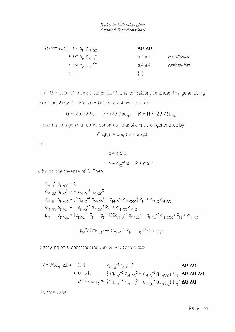
Topics in Poth lnicer s i ion’C jnnnjrj/ TrODrfiip/Ti--It/W?J

mm'QQ A Q A Q

1/2 D,.** i’j Pmp

JQ AQ AP Hamiltonian

/ * r»» / *“t p«v* Pmpp

AP AP contribution

) }

For the case o' P O inf c -•2 r\ »•% r Cl! lU i \ i r - ‘ f r ^ n c f p ri i •_ (_i 1 i U i i 1 i mat' CZO

consider the q

■" 4 . n * -1 n U r . 5o as shown earl i tr i ,

Z 7 / O P ) . D = idF/boX, K = H X ? A £ " / >4- \U r / U / r-.q T- ■ K L q p

<2 i n r> t nL ' l i i l 1t canonical transi: n r r nw i 1 1 i Ci M I 'n n n a n p r , r ^ p ' i h \ /mi 1 L*^ 1 . 1 1 ui J_ C v-» y y

Fin, [ 1 11 r D ir , 11 D - r ^ i . ; vx i q ; l ; #l!

n = n { n i\a , i i

P = q . ^ C Q . D P + C K Q , t )

q beinq the inverse of 6 . Then:

-i(-j >Q Vf-jjQQD,, ,f p

(}

^/r’Q ~ 'T'1-’Qu”,.~i * * ■ . j J « “ " 1 (“• • • ) n

Mm »q '- 'M ’ Q Q >q -if-1 »Q Q - f - v Q ^ M ’Q Q C h S r P Q Q

C'n‘QQ Pm-Q ~ ~ * Q-SVQQ t '!MjQQypnori = in - ip + r ' hPn r. 2 - n -2 n '■ d(-1 J f"jfj '• —!f-'l ;Q 1 f---| H M 1 •‘-'-IN1 jQ -fM j Q Q -iIfvj jQ j.j QQ-' ! f--]! -1

f ( O H -3H m j rw~\-

r i -t i- 1 p

nJ0. M/ " ) n n t i/ / 4ii 1 il •

l. ci11 v 1 nq (ji i!v L-uiRridiilinq sorgcr l/ *_0\ rn*o —y

/Ti K(0MiA f = '/4 n -2 r 2"M’Q *iM,QO.

4- \ / j \?ni * f /Qi JL± L / U i i i i Um i ,

i 1 w:\-i

-4

■ i n iMmA Q A Q

A Q A Q A Q

> l Ms-/-> Mm jrrs Mm jn• ; i j ■ ; »_/. r.,,crf,S P, 2 AQ AQ

r». f r\ ] r r * j r C ‘

P2 ro


i = e!' !i,/!:i:b rV L i n \ , _ , I .. f l l . t _ j (dU(j)dPMlj)/2Tf i i)j= i ,N-

n

!n- ^ J

(• + Jacobian stochastic terms + 1/ To Action

exD[i/ni Pt.m:)(Q(k)-Q(k-i)} + (a„„rA&)PM*&J/2m(e*.5 +...i‘ i ! i ■ U n ’> i

)& t}]

A r\ Ha r r\ rr: •“ r- Ci Ly \T \JI i »tJ Uii u u i i i i i - j c.

j = ei/?i CFb - f ) Limf. I l l (dOmdPmo/pTilo)J ;-i v_i J n J

n 1/ n V (Qv(k 1) At )K=l ,N

exp[i/M PM(k)fQ(k)-Q(k-u) - (qM.0-2(k)PM2(k)/2mi‘cw m. }A t}]i i . ;' ■ ; '■ *

evaluating the integrals to order At (see appendix, with a=m(qr.1)qM>Q21

function of Q,t only) yields:

iAAt/4m(QM) { n - 4 n 2i i -Q " n ■ G o

O n - 4 r 2 — H - 3_ ) L L -! ! 'Q H M JG Q

C m ,■ \jm C m .1 p.^.Q j

O n -4 n 2 _ rf - 3 n 1 ^JQ Mr i jQQ Mm ,iA ’r-vQQQ- '

I I I V U« * <-i J » • or. i~T~ n ~0 «— / " l ; < A • A f P . P s-\ i f—. . « p , i • • t t t> •— j—. t—. . £wiiCT t i i i \ ^ i ! L Cii Lj CJ '-w , l i t t Ct w , Ci ic3 L Li i i 3 L L i 1 3 1 i l U u v 3 Ci U i L U i

the mid-point prescription under a general canonical transformation. This

;o uecdUSe, uy tne group properlv, a general canonical transformation ma\/

into successive q and p transformations. 7:-■pr nr~‘

Li Oi I Jl UI^ r \ A r\ r~~ t* e* ***\ a .*~v ‘ i ^ r*. * r~, • f- y~, s—, » ~-s -. Zj U u> I u j H C u i i UI I » L * i t * 1C’ i Ci i L* \ lJ \J i 1 I l. J C1 d * 1 O i \J 1 i i 1 Ci 1 v i i y

Paqe ! 29

0 iJ Q H

'SLUJ01 D1 \ i n q UUL4:^C OL* OC/ JOUOLI

V K ELLI JOjSUE R : ■»*! iw \J t_ \J d I ? ••u

/ i? i/iw /vLLL: Ujh l i t-//U Q iiSJu9lU j Ljf&,-f Ui SOiG0_[

Tip ics in rdfh in ieor at iontCnnonica! Transformations}

S VIII General Canonical Transformations

mince no extra potential term is generated for the symmetric scheme in

:s no contribution Generated

i and trivial Ptarn lit r\ i *5 r\U : i id) i

: - 1 - - ~ r-. ~ f* p. r* r-~; ~ 7 -i /“. L 0 ;; u i;:. Cl i Li di S Z3-1 Ui i i id L i U * i

f~ ~ 1 f p n ! u. a i Li c»ii s format'ion vi.a the

?e see 1ndlrectly K - -Li id L there

r ■ > t*»“ n c f n r m m i r-i>_■ i_i i ii i _? i U i . i 1 '_i L ; Ul L

; 0 p f h, p — a r\€ a phy { Q jA '■

f A *■ \ 0 f \ n 'i ; •i the pathHamiltonian (one for which HM Is of or

Integral), and here it Is understood that only canonical transformations

that generate such Hamiltonians are considered.

Having achieved a Hamllton-Jacobi transformation one is lead to the oath

kvn n ' In n r ) = g’/,n r h mi kVn p f If) d t )b-“ b!

\ hj j * i i 0 *

• ; ,• ; t h l ■ ! = | I j ( n f V s J r; \ 1J J ‘J -P O' Ti - »-* • ! :!“ i i

II exoM/ti { PM(k)(Q(k)-Q(k-n) \)i- = i n.: ft

- U J 5(P. ” P )b s b a

cr; thp amplitude becomes mmnlv'-• / Ti ! r P” “ •* h r 3j

where r -s a generating function of the Haniiton-Jacobl transformation,

and the new coordinates (Q,P) are constant (determined from the end

ccndltlons c: g,p). This is not a physical quantity Cc.f. coherent states) and

Daoe !

topics in Pstn integration(Canonical Transformations)

'p converter! to -?r\ i t ' lHp h i i ;-yut L/t

O

Topics in Path /nfeorstion(Canonical Transformations)

SIX Conclusion

It would seem that within the symmetric scheme, no additions- terms ar

generated by a genera] canonical transformation. This was

demonstrated in the case of a point canonical transformation.

m is suggests that the symmetric scheme is

prescription i.e. pictorially.

canonica. :y

■ svn] ; ; 1 ;SAfji iU il :

Original

Theorg(C la ssica l)

H (q ,p ,t5 1

4 ■

_ midpoint quantization"

Quantized |

Original Classical TheoryH (q.,p ,t) 1

canonicaltransformation

can^ticaltransformation

+

Canonically transformed Classical Theory

K (Q ,P ,t)

midpoint ^ quantization"

4 i (iw o) m

1 Transformed !

Theorg 1

(Q uantum ) i

| K (Q ,P ,t) 1

; ' ~ — 1 1 /*<; i : r- r\ ~ ’ t_ - *■ r\ “. . ; : r. i ; i U vv z< d t u i ; 3 i d ‘_ c i i i quantizat ion or a c lassics 1 system reg ardless

whlch canonical variables 3f g I J S 0 G 1n Its descrlDtlor , as well as the use

- 1 . C . : : V . i i , : i Lj . . i_i ; : . 1 . ■_ i i Jacobi tra nsformatlon in qcar,turn meet•anlcs.

!t should perhaps be remarked that the mid-point rule is favoured (no

compelled) over others, in that It generates no additional terms during th

canonical transformation. Note however, that to get Into and from th

bcneme, s locna b l i l rn Ccinib dppear. ine vi* <_ue or nu l e r n,I \-i w W l i J

occurrina durlna the transformation is that the Hamiltonian Is the

Topics in Pdih inteardtioni;~.jfi-jr;''r&f! Trans! rmn*i nsJ

i—‘ 3 rn i 1 f n r\ — Ic s rn h i f r-^ n ct r irm r»f ’ nn T h e r\fi s : i i ! ■ j u l u - . ' l u l ! j i i i u ' . i U i i. , i cC U p cJ; •_» • ;«_ tr ••_■ i

■ v r. r- K

y’3.iz6G Dy the

ic te rn s during tne transform ation would spoil th is attempt (see

i n ; t p h p | O W •.

Operatorformulation

H(q,p> \ /Operator

formulationK(Q,P)

(mid-point) (mid-point)Path Integal a ... Path Inteqalfo rm u la tio n fo rm u la tio n

Hm(q,p) I Km(Q,P)

I Path Integral formulation

/ \H ( q ,p )

induced terms

No induced terms

Path Integral | formulation I

x {n p * ' «. L/_ ,t j

The Mid-Point Crossina

il lb atbu no l Li ear Wivan a l a n o ru l a i l \ anbiOrnidLicn ib uutbiQe ui • \ 0

iihG-pomt sciieme.

i nat i.iiib blh0mg is so wen ueiidVGG anu wuu;u seem to oe tne niannei ui

startiisa DOnit ioi rnok.inq the oain in10grdi a wen oei Ined i n d l n 01 > s a l * 0 a i

001eot / D c j u D i P c h / p s n z i u i \ i d i / G p t . / ' P o d / , tends to iiiUio.ato tnaf it 11

D o > <j ! i os tne path 1 ntears•.

Topics in Path integration(Canonical Transformations}

AppendixWorking out the general Gaussian in tegra ls

by d iffe ren tiating (w .r.t. v or ji.) the baussian integral:

I .. i II tdU(j5GV(j)/2H n j e xp [l/h E , . >,{vik}U(k) - V2(k)At/2G{ + VUfk) liV(k)}]{= | K[- '! k- i

= expH/ n i v2 At/2a + v|i ]■

U > ic i I i d y U b V e i U U

Integral =

[.. i l l (uU(i)GVi j)/2lt i \ j integrand 0Xp[]/n 2, , V(k)lKk) - V2(k) A l/ s f l }j' 1=1 ,N-1 ‘ *

Integrand Integral

I !vux/Hi ,

r;

■Ch/i)

vu*-> ->V IT

vn!_b (nio}

■(Vi) At/a

t ^ ~y

u3w,,3

V2U3, ,3, ,3 v U•/Hi ,3 / r-. X /* \V } \ L *-? /

f)

3Ch/!)2 At/a

,/u 3

iJ snp

/ o p ? C 5 i n P d i n i n t e n t e t / o n

(C a n o n ic a i T r a n s f o r m a t i o n s )

■ !- r- f -; Ui i.; n,These expressions continue to be valid to order At If a 1-

Q,t; since :o this order they may be held constant at the mid-point value.

Further, 0/5ji(k))v - (d/d^(k-n)v = At(d2/dtd[i) induces a Av, and since all

currents are held constant (at zero); so the contribution of Av coniainino

term s is nu.i. ; l !MLbLi! such as these that ten us that u (a Q)

cun‘_rluul0s wi>j > strenoth ordei \ A t a n o v \P • at os us> v At j , exceut-nQ

that tor the presence of v s (p's) only (no u’s cAQ's)) the contribution is

2PP0 when the currents are turned off.

Fponp f h p p p ? r n ; jp n p r^ c . n n p p n p p h . iripQ th p * - t h P Q fo p h P tp fU p f p r r p p p r p y i Hi !p h /

are ah those that contribute to order At.

u 00

Topics in Pditi s nicer st ion (D im e Q u s n tiz n tio n J

our

J r o c e J u r e

Pace ) s i

Topics in Path integration(Dirac Quantization)

Dirac Quantization( the method of classical endiogy)

• n this work, which is based on a paper by Chernoff [19811 the Dirac

quantization procedure is reviewed and derived from basic postulates, and

the resulting ambiguities pointed out. This Is relevant to the task of

performing a canonical transformation In quantum mechanics; for If a

quantization scheme is ambiguous, one cannot use It to induce a quantum

canonical transformation from the classical obiect.

Dirac [1958] indicates how a quantum theory might be induceo from the

classical theory in its Hamiltonian formulation. It is perhaps interesting

to note how a formulation so well suited to classical mechanics, namely

the Hamiltonian (or modified) action principle with its use of action,

Hamiltonian and phase space variables, should also oe so suited to the

quantum generalization; be it canonical or oath Integral Quantization.

Motivated by experimental results, with the need of a superposition

principle and probability amplitudes, Dirac [1958] was led to representing

siates oy vectors and observables by operators. Having got this far, one

nas still to determine the evolution (or dynamics) of the quantum system.

An analogue with classical mechanics Is most easily made when classical

mechanics is displayed in terms of the Poisson bracket, which is defined

for two classical dynamical variables by:

whore

fu.v] =

nls quantity Is

(du/hq)_(dv/dp)q - (au/ap)q(av/dq)p

independent of which canonical coordinates (In this

case q ana d ) are being used [Goldstein, 1980]

blnce the Hamilton equations of motion may be written as:

Pnoe

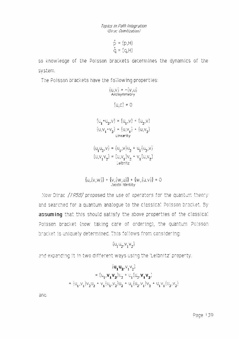
Topics in Hath integrationWirac QurnttzritonJ

P = IP;H]

Q = lQ,Hj

so knowledge of the Poisson brackets determines the dynamics of the

system.

Tne Poisson orackets have the following properties:

iu?v) = -fv,ujAntisymmetry

tu,c] = 0

{ut*u2,v) = CUj.v) * [u,,v][iJ.V V,] = [u,Vj] * fu,V,]

Linearity

{u,u2,vi = [Uj,vju2 + UjtUj.v)tu,VjV3i = iU,v,}v2 * vyu.v,]

Leibnitz

\u,[y,w]} + {v,iw,u}} + {w ju.v}} = 0Jaccbi identity

vow Dirac 1/958] proposed the use of operators for the quantum theory

and searched for a quantum analogue to the classical Poisson bracket. 3y

assuming that this should satisfy the above properties of the classical

Poisson bracket (now taking care of ordering), the quantum Poisson

bracket is uniquely determined. This follows from considering:

RyVv'jV,}

and expanding it in two different ways using the ’Leibnitz' property.

{UI U2 'V1V25= -2 + V ”: V1V2;

W V J V2U2 * V {Uj .Vj JUj ♦ UjUij.vJVj * UjVjfUj.v 5

anu

*J g 0 o i jjQ

/ opice in Path integration(Dime Quantization)

Hi U V V 1 - i 2 ! l v2

= (UjUj.VjlVj + VjCUj Uj .Vj]

- " Vj IUj .vJ u, * VjUj IUj.V ]

tquatmq these leads to:

{H1,v1}(a2v2-v 2u2) = (L1v1-v r i )[u2;v2]

Since this condition holds with ut and vy independent of u, and v„ we

have.iu1,v1] = ilhfUjWj}

LU^vJ = i n [u„vjA. M ± ±

where h is a constant determined from experiment (the case of n* 0 can

only be satisfied oy non-commuting variables). In this way we identify tne

quantum Poisson bracket to be commutation, an operation wnicn also

satisfies tne other Poisson bracket properties, if it is then furtner

assumed [D/rac, I958J that the quantum Poisson brackets obey the same

equation as the classical Poisson brackets; the quantum dynamics is

specifies (see below), and a route to quantization formulated.

To demonstrate that this quantization scheme is in fact amoiguous,

define the 'Dirac association' E) as:

Quantum operator e © (Classical object)

The postulate motivated above (PI ) then reads as:

Quantum operator commutator = if* © (Classical Poisson bracket)

Le. [Q(f),Q(g)J = i * Q{f,g)

ana aaoing one further assumption (P2)

© (i ) = T

The above postulates specify directly only now to obtain the quantum

operator for 1, and one might presume that it is necessary to separately

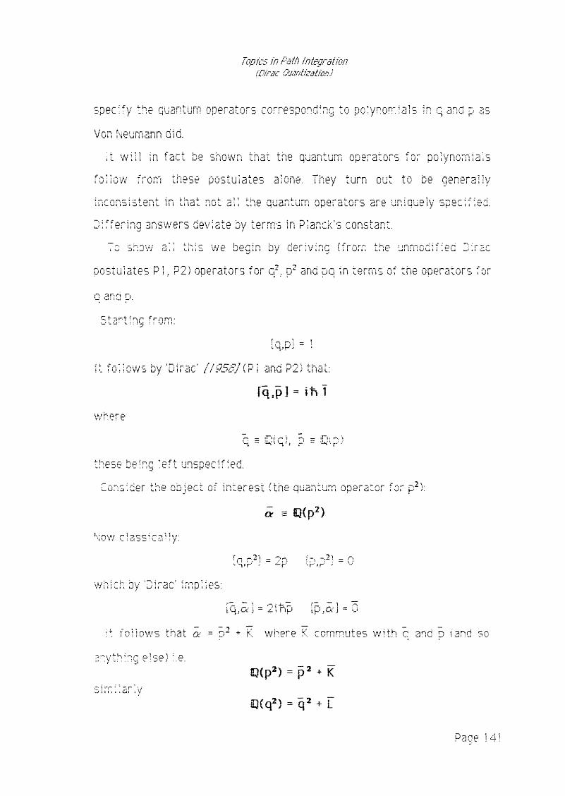
Topics in Hath integration(Dirac Quantization)

specify the quantum operators corresponding to polynomials in q and p as

Von Neumann did.

it w ill in fact be shown that the quantum operators for polynomials

follow from these postulates alone. They turn out to be generally

inconsistent in that not all the quantum operators are uniquely specified.

Differing answers deviate by terms in Planck’s constant.

To show all this we begin by deriving (from the unmodified Dirac

Dostuiates P I, P2) operators for q2; p2 and pq In terms of the operators for

c ana p.

Starting from:

iq,p3 = 1

if follows by ’Dirac' [1958]\? 1 and P2) that:

fa .5] = its Tu r n r \ r aW ! t

c = Die), p = Oyip)

these being left unspecified.

Consider the object of Interest (the quantum operator for p2):

& = U ( p 2 )

Now clsssicaNy:

iq,p2j = 2p {p,p2} = 0

which by ’Dirac’ implies:

3 = 21 TSp tima-j = C

It follows that a = 5 2 + K where K commutes with c and p land so

anything else) i.e.£!(p2) = p2 + K

Q(q2) = q 2 + LJ i l i n . \

U71PP

Topics in Path integration(Dirac Quantization)

Now to determine EKpq) In terms of p and q, look at:

'j *>G-CUpm — “SUG

! Ot

C = iLj ( p G !

f h on h\/ ‘ P» irri r - ' ■i-i i “ i : i-< V i i i_iV. .

LG + l ,p + k j = mhq

since K and L commute with q and p, they mutually commute. Havinc

dSbumea inat they, nre an variables, are a function or q and d aione. irw

Is seen bv Taylor expandlna one of (but not both) L or K.

i.M , J —T I l

UiQ/Pjp + QPLU.pj + piGjPHu + ! G ,D jDG = 41 n£

Of,-- x - ,-r \ = A f — '-ir'1 ' K'-i; rU

I U V i i i \ . i

L U, P J i "t i 1therefore

EKpq) = (pq + qp )/2To further determine (Q(d2) consider:

■ r -vrwhich by 'Dirac' yields:

, — r ■tpmqj

i. (pq + q p // G,p + i\ j - a.] + r-

IpQ + q o ,P 2]/G = G iih ip2 x K )

rq - p P x P.%- m + r~, v „2 w o - i ~ 2 , •\\ : *

' h p r c f o r p

2b* = 2(b2

u

Q(p2) = p2

Uvjffa j P'2

/opics in Hath integration(Dirac Quantization)

0(q2) = q2

Q(qp) = Cqp + p q)/2

From this follows the quantum operators for the higher polynomials in q

and d . Although it was realized by Groenewoid (1946) that starting from

(Qip2) = p2 and Ej(q2) = q2 one could develop quantum operators for other

polynomials, these starting operators were given as a supplementary

postulate to PI and P2. Here we nave shown that they in fact follow.

To expose the Inconsistency we follow the work of Groenewoid (1945).

Ambiguities arise when determining operators corresponding to higher

order polynomials. This line of argument may be continued to determine

the operators corresponding to higher order polynomials. For example:

[q3,q] = 0 ;q3,p] = 3q2

leads to:Q(q3) G + J

where J commutes with q and p, and:

"i r.-q i"-. 1 i p c K qs -

sim ilarly

[q3,pqj

C iq 3) = c 3

Q(p3' = p3

Q(pq2) = 1/2 (pq2 + q2p) f

Q(pJq ) = 1/2 (p 2C qp2) f

with no ambiguities arising up to this point.

Problems arise wltn terms such as q2p2 which have more than one

Poisson bracket origin:

i/9 {Q3,D3} = Q2r>2

:/3 [pq2,p2q) = q2p2

Pace 14

Ton/cs in To in inioordiion (D ir a c Q u a n tiz a tio n )

wirch each lead to a corresoondina ooeratcr

T-.2-.2 M Msnti

- *v- nltu* i i nnn - */. ‘ n r

wh 1 ch til f ♦! i er by > n, 2 '"iU\ h /.

1f ; i i’j 1i i i f h i c 5> . m 3 way that. rsi i i

ambiquoUS (or inconaibterit).

i ii If Q i i i ctirence between ti 5]

d ■; n SUl I'V4 1) \A/ C l pQ V v u l • - npfirlQd pci i C u U U U C i - J ' n ■Mi

\J» I

jJU .


References

Y.Aharonov, C.K.Au, E.C.Lerner and J.Q.Liang, Phys.Rsv. D 29 ( 1984), 2396-.

Y.Aharonov and D.Bohm, 'Significance of Electromagnetic Potentials in the Quantum theory', Phys.Rev. 1 15 (1959), 485-.

5.B.Baker andE.T.Copson, The Mathematical theory of Huygens* Principle', Oxford at the Claredon Press, 1950.

H.S.Carslaw, ‘Some Multiform Solutions of the Partial Differential Equations of the Physical Mathematics and their applications', Proc.LondPIath.5oc. 30 (1599), 121-.

H.S.Carslaw, ‘The Green's Function for a Wedge of any angle, and other problems in the Conduction of Heat', Proclond.fiath.Soc. 8 (1 9 1 0 ) , 365-.

H.S.Carslaw, ‘Diffraction of waves by a Wedge of any Angle*, Proclond.Math.Soc., 18 (1919), 291 -.

P.Chernoff, ‘Mathematical Obstructions to Quantization', h'ad.J., 4 (198 *), 379-.

R.E.Crandall, 'Exact Propagator for Motion confined to a Sector', l.Phy.A. 16 (1983),

I. Daubechies and J.Klauder. 'True measures for real time path integrals', in 'Path Integrals from meV to MeY!, Ed. M.Gutzwiller, A.lnomata, J.Klauder and L.Streit, World Scientific, 1985, 425-.

C.DeWitt-Morette, Phy.Rev. 81 (1951), 848-.

C.DeWitt-Morette, S low , L.Schulman and A.Shiekh,‘Wedges !', Found ofPhys. 16 ( 1986), 31 i -.

P.Dirac, 'The Fundamental Equations of Quantum Mechanics’, Proc Roy. See. A109 (1925), 642-.

P.Dirac, The Principles of Quantum Mechanics , 4 th Ed..Oxford, 1958.

J. Dowker, 'Quantum Field Theory on a Cone', d.PhysA 10 (1977), ! !5 -.

3.F.Edwards and Y.Y.Gulyaev, Pro.Roy.Soc 2 1 9 (1964). 229-.

S.F.Edwards, ‘Statistical Mechanics with Topological Constraints: I ', Pro.Phys.See 91

( 1967), 513-.

R.Feynman, ‘Space-Time Approach to Non-Relativistic Quantum Mechanics', Rev.Mod.Phys. 20 ( 1948). 267-.

(reprinted in 'Quantum Electrodynamics', Ed. J.Schwinger, Dover, 1958.)

'"'3Q0 ] <43


R.teynmen, QED, The strange theory of Light and Matter (M ix O.Mautner memorial Lectures) , Princeton Urnversiiy Press, i9ci"o.

R.Feynman, 'The Feynman Lectures on Physics', vol 2, Sec 15.5, Addison Wesley,1 963.

R.Feynman ancA.Hibbs, 'Quantum Mechanics and Path Integrals', McGraw-Hill,

R.rdneHt, canonical iransiormationsandPnaseopscePatn integrals , u.Nath.Hnys., IT( « o~?.c / n n

C. C.Gerry and VASingn, Phy.Rev. D 2 0 , 1 0 (1979), 25b0-.

J.Gervais and A.Jevicki, 'Point Canonical Transformations in the Path integral', Nuc/.Phvs., B IO (1980), 93-.

H. Goldstein, 'Classical Mechanics', 2nd Ed., Addison-Wesley, i960.

i.S.Oredshteyn and l.M.Ryzhik, 'Table of Integrals, Series, and Products', 4th Ed., Academic Press, 1980.

H.Groenewold, 'On the principles of elementary Quantum Mechanics' Physicp 12 ( 1946), 4 0 b - .

J.Jackson.'Classical Electrodynamics', 2nd Ed., Wiley, 1975.

A.Kapoor, 'Quantization in Nonlinear Coordinates via Hamiltonian Path integrals', Phys.Pev.,D. 2 9 ( 1984); 2339-.

J.Klauder, 'Path integrals’, Lectures given at XIX. Internationale Universitaiswochen fur Kernphysik, Schlaaming, Austria, 1980.

n.^retzschmar, Aharonov-tsohm Scatter ing ol a Wave PacK.et ot r init© Extension ,ZPhysft 1 85 (1965), 84-.

L. Landau and E.Lifsnitz, 'Mechanics' . L.U. , Per gam on Pr So o, i z- 3 2.

M. G.G.Laidlaw and C.DeWitt-Morette, Phys.Rev.Lett 3 (1971), 1375-.

F.Langcuche, D Rcskaerts and E.Tirspegui, Functional Integration and SemiclassicalExpansions', Reidel, 1982.

H.M.MacDonald, Proc.Lend Nath.Sue., Ser.2, 1 (1904), 393-.

H.M.MacDonald, in 'Electric Waves', an Adams prize essay, Cambridge University press, 1902 186~.

D.McLaughlin and L.bchulman, 'Path integrals in Curved Spaces’, J.fiath.Phys. I i 9 t O /, Z ‘ j z 0 -.

Pace

1 2


5.Mandelstam, Ann. ofPhy. (N.Y.). 19 (1962), !-.

i.Mayes and J.Dowker, 'Canonical Functional Integrals In General Coordinates',Proc.R.Son.Land..h.'SH (1972), 131 -.

'.Mayes and J.Dowker, 'Hamiltonian Order inqs and Functional Integrals', J.Math.Phys., 14 (1973), 434-.

O.Morandi and E.Menossi, 'Path-Integrals in Multiply Connected Spaces and the Aharonny-Bohm effect'. Eur.J.Phy. 5 (1984), 49-.

S.OIariu and I.Popescu, 'The Quantum effects of Electromagnetic Fluxes', Pev.Nod.Phvs. 57 2 ( I9 S5 ), 339-.

W.Pauli, 'On Asymptotic Series for Functions in the Theory of Diffraction of Liaht’, Phys.Rev. 54 (1938), 924-.

D.Peak and A.inornata, JMath.Phys. 10,8 (1969), 1422-.

L Schulman, Techniques and Applications of Path Integration', Wiley, 1981.

L.S.Schulman, 'Exact Time-Dependent Green's Function for the Half-Plane Barrier', P hyR evlett 49 ( 1982), S99-.

L.S.Schulman, 'Ray Optics for Diffraction: A useful Paradox in a Path Integral Context', in 'Proceedings of the symposium on Wave-Particle Dualism ', Perugia , i 9 o Z , x5c>-.

A.Shiekh, Ann.Phys. 166, (1986), 299-.

A.Sommerfeld,'Mathematische Theorieder Diffraction', tla th .A nnA l (1896), 31 7-.

A.Sommerfeld, 'Optics', Academic Press, 1954, 247-.

L.Van Hove, 'Sur certaines representations uni tares d'un groupe infinl de transformations', Proc.RoyAcad.5cL Belgium, 26 (1951

Page 147


a t tAee ama- a- eciA-a te/TvctA-ta c-iswt- a- tat aj; iÂawna, a/net with i t a-

tat p*j§pi& ta Vk-o.srJi-.

)t iA- to a^v a-ciAimA>6^f^^nwrit t f t a t d tm - a a t- m w t

t lle Cl'TVy AtIWl-, fcut .

i j Oe -VA 'M btiAAO stty- VdA/Jh TiW ©fWlA &A-0/ITV, V3$\& lla 4 tfie

w ttu e [w iiw ri^ w M j ailW vtiO a£ a-ttaus-l/n^ <>tua?-ertit a- imoA-UA^cE a/mau-'nt

€*P pimdma - t a t a a d e t k jsaa- ©û m v a - t f e a / ^ . i F W I t a a * f e a ^ c y i w ^ c E a u ^ a a - r u c e a - i v c i

•MA^be t, cvTvd eA 'j^ aall4 j- |oa altatw Ai^ 'me tile a^|>Mtumeti;}- t© at$>ti£

'm/yaet-l t© tfie aettvrti> a4> © a.' atia iW t vahtAriPfyvp Bapiîaareat. ‘J © tecale

£)b'XxkJ[&-JV{j&A&to -1A>1W, ItflUte Â-i.-ti./u/0' feÂi-at-., t©©!- VuV, lAite-eat t-A- T:14j-

vrtA- iAecE (<fA©*$e) -me t© tf©- 'n w , aati- iw vtecl me ©ut t© <$-uet/rv ta'i-

ata earT^teticm' J^kvivy- tiWafe© t© all- tA©ie mamy- ;4e©£>e© I am a

■MA-meaMe/AtE'U- hÂrndwt {b -, a t amcB jmam c fe -k ^ *9&7vcf.t© °j Eaaaiiea, a-

P ) Tna-m aw-ft© ^©liteay- oammemtecE upw\, ixmA cAittcaAecB -ttfliat a t t-ne

tame -u>aA- (amx ■pvvtxrcp'C a-talt c-a] a <4t©adt|- âece ©p -mij- v&m&,

f <£ki, •fi-c+iAA-- ak%eA wA^tUvcj' t-Raa- ac-l/Ai vjl€,<lc|£/mP/r^ a t m w - Ma^cpctect t f ia t £ a . itaay-SeA m tsj&t Ibe m i* e^ctevnat exa/nwneA-. fTfi.ae- fcpAAa tl\e c fiA , 3 t€A ‘v+j a t t© le e im a ^ m a ta a a a-e t© m t a t I maa* ft-ave ©Mattm ,

cPfi4AA-i-c-iA-tA- 8t£e m©<t j ea^te, (©al-t| pon&jz/p awm©}, iem t t© £>e a

m©©<£y arnct vrv&eGune tat, o a /A d <A©iitc£ tale ta t la a ^ 'nvy- PpM ik v -

<K.ademta ta-at ellaA ea a eaanp ^ laft (|a4 tnela i>atienee, apati-A? a t t-aa

aacB eAea lecyuervt aiAâc-U-aPva). t HeiAA- wcw- aat a/n ea-v^ tae&.

h!2O0 1 4


to£m ati-ao OT.& a-o- u4vUd^- a-ad p 'l& tiû c ia ^lodii-c-im}- a-o

•m-

Joa- me, a- P&QA& to eoca^je, -ia Wtv t#v& IW odd êt ’qood1.. 11 tda'rv&

tft-e da-fjJ of- tR-i-nd ijm-a- fa d $& w i« jkiemd&tf- amd Re£^j5td feu/ncft i-t-

i Aôufd do fva-ad to tW d.

Jo tto ma-mu- merntmo- of t id a-di-o^R-^-oioo qAou£> a t Em ^ ii-aR -usdA

ooftom U t*M& R ad ofco e comnÛoao, an d tR& RnaR. eaeA /i ^vyoi-oo s u p

?,om t& at feundeaed dy- mm- ao 5 tot-£sd § m tft-i-o tim-tima-.

J o Idnoum o&îAâttoaciooot'Ci- an d a-6ife •■iu-a-o a

oo&s/a/ru tinopziiAmss, to am an-not amt tPuÂAsl -Mi-ott G4 J

5 am fontuma-te to fee, a-M& to oan.}- tR a t V lw w a/te oo mamy- otIWt-o to

wftem a oa>e-, an d Ro£>o ono da-tf to aoim-a- ttWm, irn moae tR-am la o t

■u*n-itt€/rv tR-aaRx

Jo t)a ^ id J 6a-t'Ki- w R a tooi- am inte/ie-ct yrv tR ix tRxoix a x i t w doi.mx

W ii-ttoa, pucm d u p tRo m axx conmptx xo muxR- faxtai- tR x a 1), a-nd made,

tto xx^c-avrv dstaxEx not otta/i-ty- j txxwntnd. cMoae nncemtty- an d in

connection -us-ctR- i&& lAj-a-itony- of tn-ix tRcxix, a xRotdd E iie to m ention

fy/Tid tand-nx, a aem* otaciki/nyt -tofio cRec-ied come of m a ca-coata-ti-onx

am t odioxe ent&uxtaxm 1) Rote neovt- jd.odtmo-, a n d jje/iatd §bwim ton-

R-ix commentx, a-£R to often ôoi-teRy- |:>ointi-mt|- o at come fa-id t in nvy

anqiAmentx JR en tRene ix- 3a.m JE a ttid a a , caitR out adi-om- tio xv/ni.aax

COufd fee oonfxdened com pete D ii-Re m oot fen fW/i-i-ny R-tx

p 4&r®, a-ad ended o i| acti-^d-^ ^R-iag- i-t

Ji/ria-tt-U' ot cotiwo- to ^ lo o o ao defcto o | y ta U tiid e Jffcne 3 -diou-td tOm

to aoRaoudodê ôiiooaa Jl-oS-R-ta-n-i- (-loRoao aorris 5 m w i- cou-td q^ dt)

a/nd -udt,o p o /i? v a ^ oa>lod oaco too oft n- adou-t t ld ^ 10^1000 of m a

ndooi-o, d id -tAKi-o a jdi€md tfd1-0ii4 Roi.it ooi-i-oia/fq taad i- you-

D pi n p i 4-MI W *W» W 2 --


Po/ihap'^ £ c wf a- ^ caubtOT* ts m& e/miba/iJk/n

\ t fp m , top tlta m€Kyt cEi JJu>u£t ^

t&e. p a x & &$ a & &j$fo&wci te y p a A o . 3 t to-

m<ytj. pyv a* i& Ma/rrte tftemrto&Ew* £©*,• w-Pvcvt €£/ttk>- a- Ixm4 ^

t o p i c s i n - spiral.imperial.ac.uk

Documents