T H E U N I V E R S I T Y O F T U L S A THE GRADUATE ... Dissertations/Hadi... · erosion prediction models such as Computational Fluid Dynamics (CFD) based erosion models and Sand

T H E U N I V E R S I T Y O F T U L S A

THE GRADUATE SCHOOL

DEVELOPMENT OF EROSION EQUATIONS

FOR SOLID PARTICLE AND LIQUID DROPLET IMPACT

by

Hadi Arabnejad Khanouki

A dissertation submitted in partial fulfillment of

the requirements for the degree of Doctor of Philosophy

in the Discipline of Mechanical Engineering

The Graduate School

The University of Tulsa

2015

ii

T H E U N I V E R S I T Y O F T U L S A

THE GRADUATE SCHOOL

DEVELOPMENT OF EROSION EQUATIONS

FOR SOLID PARTICLE AND LIQUID DROPLET IMPACT

by

Hadi Arabnejad Khanouki

A DISSERTATION

APPROVED FOR THE DISCIPLINE OF

MECHANICAL ENGINEERING

By Dissertation Committee

____________________________________, Chair

Siamack Shirazi

____________________________________,Co-Chair

Brenton McLaury

____________________________________

Michael Keller

____________________________________

Kenneth Roberts

____________________________________

Selen Cremaschi

iii

COPYRIGHT STATEMENT

Copyright © 2015 by Hadi Arabnejad Khanouki

All rights reserved. No part of this publication may be reproduced, stored in a

retrieval system, or transmitted, in any form or by any means (electronic, mechanical,

photocopying, recording, or otherwise) without the prior written permission of the author.

iv

ABSTRACT

Hadi Arabnejad Khanouki (Doctor of Philosophy in Mechanical Engineering)

Development of Erosion Equations for Solid Particle and Liquid Droplet Impact

Directed by Drs. Siamack Shirazi and Brenton McLaury

146 pp., Chapter 8: Recommendations

(475 words)

In the oil and gas industry, there are many particles that may cause erosion. These

particles are of various sizes, shapes and hardnesses. Liquid droplets are also another

source of concern, especially in high velocity gas streams. Currently, solid particle

erosion prediction models such as Computational Fluid Dynamics (CFD) based erosion

models and Sand Production Pipe Saver (SPPS) program developed by the

Erosion/Corrosion Research Center (E/CRC) rely on empirical erosion equations. These

equations do not account for the erodent particle and target material properties accurately.

In this work, different materials have been tested in direct impingement

configuration, and particle velocity has been measured with particle image velocimetry

(PIV). A new semi-mechanistic erosion equation has been developed by assuming that

erosion caused by particle impacts is due to two mechanisms, cutting and deformation.

Empirical constants have been obtained for the tested materials, and the model has been

verified with experimental data for different particles. In contrast to the angle functions

that are currently being used for all particles and impact velocities, angle dependence in

the new model changes with the particle shape and velocity and showed fair agreement

v

with experimental data.

The effect of particle hardness on the erosion of stainless steel has been studied

with fine particles at low impacting velocities with two experimental apparatuses,

submerged configuration with slurry mix and mist flow test with solid particles entrained

in the droplets. The testing particles are iron powder, calcite, barite, apatite, hematite,

magnetite, silica flour, alumina and silicon carbide. Droplet size and velocity for

air/water tests have been measured by PIV for air/water tests, and particle impact velocity

for both tests is estimated from CFD simulation with particle tracking scheme. It was

observed that erosion ratio increases with increasing particle hardness when the target

material is harder than the particle and does not change considerably after the point where

the particle is hard enough to keep its integrity during impact.

A new erosion equation has been developed to calculate erosion resulting from

liquid impacts for pipeline materials based on experimental data that was collected

previously at E/CRC and American Society for Testing and Materials (ASTM) G73

guideline. Based on the new erosion model, a procedure has been developed to predict

erosional velocity due to liquid droplet impact (with or without small particles entrained)

utilizing the entrainment fraction and droplet size calculated from two-phase flow

correlations and the impact velocity of the droplets within a pipe elbow or a tee that is

estimated using stagnation length model. The erosional velocities computed using this

model are compared with the erosional velocities computed using API RP 14E. It is

shown that the trend of the erosional velocity calculated by the API guideline is

extremely conservative as compared to the new model predictions for erosion due to

liquid impacts and does not correlate with erosion due to small entrained particles.

vi

ACKNOWLEDGEMENTS

I would like to express my sincere thanks to my advisors, Dr. Siamack Shirazi and

Dr. Brenton McLaury for their excellent guidance, caring, patience, and providing me

with an excellent atmosphere for doing research. I would like also to thank Dr. Michael

Keller, Dr. Kenneth Roberts and Dr. Selen Cremaschi for serving on the committee and

their help in preparation of this dissertation. I would like also to recognize Dr. John

Shadley and Dr. Edmund Rybicki for their advices and help during the course of my

research.

Special thanks are extended to the member companies of the Erosion/Corrosion

Research Center (E/CRC) for providing funding in support of this work. The funding and

support from The Tulsa University Center of Research Excellence (TUCoRE) and

Chevron Energy Technology Company is gratefully acknowledged. I would like to thank

Mr. Ed Bowers, senior technician of the E/CRC, for providing technical support and my

friends and colleagues at The University of Tulsa for their help and support.

I would like to thank my parents who have always been supportive of my

education and for their endless encouragement and patience, and my parents-in-law, my

brother-in-law and my family for encouraging me with their best wishes.

And last but not least, I would like to express my gratitude and appreciation to my

dear wife for her understanding, continued support and encouragement during the past

few years and without her I would never have enjoyed so many opportunities.

vii

TABLE OF CONTENTS

COPYRIGHT STATEMENT .................................................................................... iii

ABSTRACT ............................................................................................................... iv

ACKNOWLEDGEMENTS ....................................................................................... vi

TABLE OF CONTENTS ........................................................................................... vii

LIST OF FIGURES ................................................................................................... ix

LIST OF TABALES .................................................................................................. xiii

CHAPTER 1: INTRODUCTION......................................................................... 1

1.1 Overview .................................................................................................... 1

1.2 Research Goals .......................................................................................... 2

1.3 Research Approach................................................................................... 2

CHAPTER 2: BACKGROUND AND LITERATURE REVIEW .................... 4

2.1 Introduction ............................................................................................... 4

2.2 Solid Particle Impact Erosion .................................................................. 4

2.2.1 Background ..................................................................................... 4

2.2.2 Literature Review ............................................................................ 6

2.3 Liquid Droplet Impact Erosion ............................................................... 11

2.3.1 Background ..................................................................................... 11

CHAPTER 3: EXPERIMENTAL SETUP AND MEASUREMENTS FOR

SOLID PARTICLE EROSION .............................................................................. 13

3.1 Introduction ............................................................................................... 13

3.2 Experimental Setup .................................................................................. 14

3.2.1 Direct Impingement Tests in Gas .................................................... 14

3.2.2 Liquid Submerged Tests .................................................................. 16

3.2.3 Air/Water Mist Flow Tests .............................................................. 18

3.3 Velocity Measurements ............................................................................ 20

3.3.1 Gas Velocity Measurement ............................................................. 20

3.3.2 Particle Velocity Measurement ....................................................... 20

CHAPTER 4: SAND PARTICLE EROSION MODELING ............................ 31

4.1 Introduction ............................................................................................... 31

4.2 Experimental Materials ............................................................................ 31

viii

4.2.1 Erodent particles ............................................................................. 31

4.2.2 Erosion testing materials ................................................................ 32

4.3 Mechanistic Modeling............................................................................... 33

4.4 Experimental Validation .......................................................................... 39

4.5 Uncertainty Analysis and Error Propagation ........................................ 48

4.5.1 Uncertainty in Velocity Measurement ............................................ 48

4.5.2 Uncertainty in Mass Loss Measurement ......................................... 52

4.5.3 Error Propagation in Erosion Ratio Equation .............................. 53

CHAPTER 5: EROSION BY SOLID PARTICLES OTHER THAN SAND .. 55

5.1 Introduction ............................................................................................... 55

5.2 Experimental Data .................................................................................... 57

5.3 Data Analysis and CFD Simulation ........................................................ 67

5.4 Effect of Particle Hardness on Erosion ................................................... 69

CHAPTER 6: LIQUID DROPLET EROSION MODELING .......................... 72

6.1 Introduction ............................................................................................... 72

6.2 Experimental Data .................................................................................... 73

6.3 Erosion Modeling ...................................................................................... 82

6.4 Application to Pipe Flow and Threshold Erosional Velocity Calculation ............................................................................................................... 91

CHAPTER 7: SUMMARY AND CONCLUSIONS .......................................... 103

CHAPTER 8: RECOMMENDATIONS .............................................................. 107

BIBLIOGRAPHY ......................................................................... 108

APPENDIX A: SAND EROSION DATA .............................................................. 118

APPENDIX B: OTHER SOLID PARTICLES EROSION DATA ..................... 139

APPENDIX C: LIQUID IMPACT EROSION DATA ......................................... 143

ix

LIST OF FIGURES

2.1 Typical erosion behavior of ductile and brittle materials versus impact angle

........................................................................................................................ 6

3.1 Schematics of experimental test facility ........................................................ 15

3.2 Configuration of nozzle and specimen holder ............................................... 15

3.3 Calculation of erosion ratio from experimental data ..................................... 16

3.4 Schematics of submerged experimental apparatus ........................................ 17

3.5 Submerged experimental apparatus ............................................................... 17

3.6 Schematics of air/water mist experimental apparatus .................................... 18

3.7 Air/water mist flow experimental apparatus .................................................. 19

3.8 Schematics of particle image velocimeter ..................................................... 22

3.9 Particle velocity measurement setup .............................................................. 22

3.10 Details of the position of camera and velocity measurement box ................. 23

3.11 Tracked particle sample (for 150 µm sand) at gas velocity of 46 m/s

(5 inches H2O)............................................................................................................ 23

3.12 Particle velocity distribution (for 150 µm sand) at gas velocity of 46 m/s

(5 inches H2O)............................................................................................................ 24


(10 inches H2O).......................................................................................................... 24


(10 inches H2O).......................................................................................................... 25


(15 inches H2O).......................................................................................................... 25


(15 inches H2O).......................................................................................................... 26

x


(20 inches H2O).......................................................................................................... 26


(20 inches H2O).......................................................................................................... 27

3.19. Tracked particle sample (for 150 µm sand) at gas velocity of 103 m/s

(25 inches H2O).......................................................................................................... 27


(25 inches H2O).......................................................................................................... 28

3.21. Tracked particle sample (for 150 µm sand) at gas velocity of 113 m/s

(30 inches H2O).......................................................................................................... 28


(30 inches H2O).......................................................................................................... 29

3.23 Particle size distribution for 150 µm sand ..................................................... 29

3.24 Velocity calibration curve for 150µm, 300µm sand and 150µm glass beads 30

4.1 SEM micrographs of three erodent particles ................................................. 32

4.2 Erosion scar and SEM micrographs of SS-316 surface eroded with 150 µm sand

at two impact angles: a) 30o and b) 90

o ...................................................................... 35

4.3 Force balance of the particle cutting into the surface .................................... 35

4.4 Cutting erosion empirical constants for tested materials ............................... 40

4.5 Erosion resistance versus material hardness .................................................. 41

4.6 Deformation erosion empirical constants for tested materials ....................... 41

4.7 Contribution of cutting and deformation wear in the total wear .................... 42

4.8 Erosion ratio of carbon steel 1018 at different impact velocities and angles

........................................................................................................................ 43

4.9 Erosion ratio of stainless steel 2205 at different impact velocities and angles

........................................................................................................................ 43

4.10 Erosion ratio of aluminum alloy 6061 at different impact velocities and angles

........................................................................................................................ 44

4.11 Normalized ER of Inconel 625 at different impact velocities and angles ..... 45

xi


........................................................................................................................ 46

4.13 Normalized erosion ratio of aluminum alloy 6061 eroded with sand and glass

beads ........................................................................................................................ 47


........................................................................................................................ 54

5.1 SEM images of erodent particles ................................................................... 59

5.2 Iron powder particle size distribution ............................................................ 60

5.3 Calcite particle size distribution..................................................................... 60

5.4 Barite particle size distribution ...................................................................... 61

5.5 Magnetite particle size distribution ................................................................ 61

5.6 Silica flour particle size distribution .............................................................. 62

5.7 SS-316 mass loss after 72 hours in submerged and mist flow tests ............... 63

5.8 Erosion ratio of the SS-316 specimens for different particles ....................... 64

5.9 Classification of the particles according to their shape (Powers 1953) ......... 65

5.10 SEM micrographs of different locations on SS-316 specimens eroded with

different particles ....................................................................................................... 66

5.11 CFD simulation and particle tracking results, a) velocity contours and b) particle

traces in submerged jet flow and c) sequences of droplet impact with particles ....... 68

5.12 Correlation between normalized erosion and particle hardness .................... 70

6.1 Two possible cases for liquid droplet impingement erosion ......................... 73

6.2 Rotating arm and liquid jet erosion experiment schematics .......................... 73

6.3 Effect of impact velocity on liquid impact erosion inception ........................ 74

6.4 Maximum erosion rate vs. impact velocity (Baker et al. 1966) ..................... 75

6.5 Wastage speed of the pipe (Higashi et al. 2009) ............................................ 76

6.6 (a) Specimen jet normal incidence, (b) 30o impact angle .............................. 78

6.7 Adjusted mass loss of the specimens to 144 hrs ............................................ 81

xii

6.8 ECR versus chromium content of the samples for brine and tap water ......... 82

6.9 ECR versus chromium content of the samples for brine ............................... 84

6.10 Erosion ratio vs. impact velocity ................................................................... 88

6.11 Erosion ratio vs. impact velocity (ASTM correlation and exp. data) ............ 89

6.12 Erosion ratio vs. impact velocity (modified correlation and exp. data) ......... 90

6.13 Calculation procedure of the penetration rate due to liquid droplet/solid particle

impact ........................................................................................................................ 93

6.14 Stagnation length for tee and elbow............................................................... 95

6.15 Sequence of simulated droplet and particle impingement and corresponding

simplified model ........................................................................................................ 97

6.16 Comparison of predicted threshold erosional velocity .................................. 99

6.17 Variation of erosional velocity versus operating pressure ............................. 100

6.18 Comparison of predicted threshold erosional velocity .................................. 102

xiii

LIST OF TABLES

3.1 Summary of testing conditions in two experimental apparatuses .................. 19

4.1 Target materials properties ............................................................................ 33

4.2 Empirical constants for the erosion equation ................................................. 48

4.3 Particle velocity measurement results for 150 µm sand ................................ 50

4.4 Effect of particle velocity uncertainty on erosion .......................................... 51

4.5 Relative uncertainty in the erosion ratio determination from mass loss ........ 52

4.6 Quantification of relative uncertainty in the erosion ratio ............................. 53

5.1 Erodent particle properties ............................................................................. 58

5.2 Average particle impact velocity and angularity ........................................... 69

6.1 Experimental studies in the literature ............................................................ 77

6.2 Mechanical properties of tested materials...................................................... 78

6.3 Chemical composition of tested materials in wt% (balance Fe) .................... 79

6.4 Normalized erosion resistance (NER) for several oilfield materials ............. 87

A.1 Erosion data for carbon steel 1018 at particle velocity of 9.2 m/s ................. 118

A.2 Erosion data for carbon steel 1018 at particle velocity of 18.4 m/s ............... 119


A.4 Erosion data for carbon steel 4130 at particle velocity of 9.2 m/s ................. 121



A.7 Erosion data for stainless steel 316 at particle velocity of 9.2 m/s ................ 124

A.8 Erosion data for stainless steel 316 at particle velocity of 18.4 m/s ............. 125

xiv

A.9 Erosion data for stainless steel 316 at particle velocity of 27.6 m/s .............. 126

A.10 Erosion data for stainless steel 2205 at particle velocity of 9.2 m/s .............. 127

A.11 Erosion data for stainless steel 2205 at particle velocity of 18.4 m/s ............ 128

A.12 Erosion data for stainless steel 2205 at particle velocity of 27.6 m/s ............ 129

A.13 Erosion data for 13 chrome duplex at particle velocity of 9.2 m/s ................ 130

A.14 Erosion data for 13 chrome duplex at particle velocity of 18.4 m/s .............. 131

A.15 Erosion data for 13 chrome duplex at particle velocity of 27.6 m/s .............. 132

A.16 Erosion data for Inconel 625 at particle velocity of 9.2 m/s .......................... 133

A.17 Erosion data for Inconel 625 at particle velocity of 18.4 m/s ........................ 134

A.18 Erosion data for Inconel 625 at particle velocity of 27.6 m/s ........................ 135

A.19 Erosion data for aluminum alloy 6061 at particle velocity of 9.2 m/s ........... 136

A.20 Erosion data for aluminum alloy 6061 at particle velocity of 18.4 m/s ......... 137

A.21 Erosion data for aluminum alloy 6061 at particle velocity of 27.6 m/s ......... 138

B.1 Erosion data for other solid particles in submerged configuration ................ 139

B.2 Erosion data for other solid particles in mist flow configuration .................. 141

C.1 Liquid impact erosion data with brine (high velocity)................................... 143

C.2 Liquid impact erosion data with tap water (high velocity) ............................ 145

C.3 Liquid impact erosion data with brine (low velocity) .................................... 146

C.4 Liquid impact erosion data with brine (30 deg impact) ................................. 147

1

CHAPTER 1

INTRODUCTION

1.1 Overview

In the oil and gas industry, erosion/corrosion may be a major problem in

production and transportation facilities including but not limited to pipelines, valves,

chokes, production manifolds and process headers. Erosion is the physical removal of

material by solid particles or liquid droplets, and corrosion is another form of material

degradation that occurs through chemical reaction. So, production and transportation

facilities are designed so that the flow velocity is below the erosional velocity,

presumably a flow velocity at which it is safe to operate but beyond that erosion damage

may occur. This threshold velocity depends on many factors such as fluid properties,

operating condition, entrained particles and geometry type and size, and its prediction is

important from both economical and safety aspects. Furthermore, erosion/corrosion of

materials due to the impingement of solid particles or liquid droplets is also important in

power plant and aerospace industries.

Depending on the oil and gas production condition, solid particles may be present

in the flow. The particles that may cause erosion are of various sizes, shapes and

hardnesses, and the effects of these parameters are properly understood. In clean service

or corrosive flow, liquid droplets are another source of concern especially in high

velocity gas streams. Moreover, the liquid droplets that are entrained in the produced gas

from the reservoir may be corrosive or contain very small particles that are hardly

2

separable by physical means.

1.2 Research Goals

The main goals of this work are to predict erosion failure in production and

transportation facilities in oil and gas industry and their components due to the

impingement of different particles and liquid droplets. Being able to predict erosion

resulting from various particles and droplets, would lead to lower costs of erosion

inspection and maintenance and also, the risk of component failure would be reduced by

improving geometry and utilizing more appropriate materials.

1.3 Research Approach

A comprehensive approach to erosion modeling consists of flow modeling,

particle tracking and erosion equations. So, the first step is to model the flow either by

computational fluid dynamics (CFD) or use approximations for flow near the wall. Then,

particles are tracked as they move toward the wall, and the impact velocity and angle is

estimated. The final step is to apply the erosion equation for the estimated impact

velocity and angle and calculate the erosion ratio which is the ratio of target mass loss to

the mass of erodent particle. The erosion ratio equation plays a major role in this

calculation and depends on many parameters including but not limited to erodent particle

characteristics, target material properties and speed and angle of impact. Thus, in the

present work, erosion models are investigated including erosion resulting from sand,

other particles and liquid droplets.

3

The approach of this work is first to search the literature for erosion equations for

solid particles. Then, conduct erosion tests in a direct impingement configuration for

different materials and develop a mechanistic model for erosion prediction which

accounts for the speed and angle of impact, particle characteristics and target material

properties. Particle hardness will be also correlated to erosion based on the experimental

data obtained in a separate experimental facility. After completion and verification, this

model will be implemented in SPPS (Sand Production Pipe Saver program developed at

E/CRC) as well as commercial CFD software such as ANSYS Fluent to predict erosion

caused by different particles in the oil and gas industry.

For calculation of erosion due to liquid droplets, the literature is surveyed for

erosion models and experimental data. Experimental data that are obtained at E/CRC are

used to develop a new erosion ratio equation for liquid droplets. Multiphase flow

equations and models are implemented to determine impact conditions of droplets and

particles to be substituted in the erosion equations to predict erosion ratio, and a

calculation methodology is presented to calculate threshold erosional velocity or

penetration rate due to liquid droplet impingement with or without small particles at very

low solid concentrations.

4

CHAPTER 2

BACKGROUND AND LITERATURE REVIEW

2.1 Introduction

In order to prevent severe erosive/corrosive damage to different components in oil

and gas production and transportation facilities, extensive theoretical and empirical

studies have been carried out by the researchers from around the world. The emerging

guidelines and erosion/corrosion prediction tools may be classified into categories based

on the mechanism of degradation: erosion, corrosion or erosion/corrosion. Solid particles

that may be present in the liquid or gas produced from the reservoir can cause erosion

damage, and the transporting fluid may cause corrosion. The synergistic effect of these

two mechanisms is called erosion/corrosion. Liquid droplets can also cause erosion if

they have enough energy to degrade the target material mechanically. The main focus of

this work is on erosion caused by solid particle and liquid droplet impacts.

2.2 Solid Particle Impact Erosion

2.2.1 Background

The approach to predict erosion damage for a desired geometry and flow

condition has three major steps: flow modeling, particle tracking, and erosion calculation.

The flow solution and particle impact speed and angle may be approximated from

5

simplified models or obtained more accurately from Computational Fluid Dynamics

(CFD) simulations. Generally in a CFD simulation of particle erosion, an Eulerian-

Lagrangian model is employed. In other words, the fluid flow solution is obtained from

Navier-Stokes equations (Eulerian approach), and then particle traces are determined

using a Lagrangian particle tracking scheme. The CFD and particle tracking are done to

determine particle impact speed and angle that affect erosion of materials. The next step

is to substitute the impact speed and angle in an appropriate erosion equation and find the

erosion. The erosion equation, which is a function of target material specifications,

particle properties and particle impact condition, is very important in this calculation

procedure.

The parameters that erosion depends on may be classified into three categories:

impact condition (impact speed and angle), erodent particle characteristics and target

material properties. The most important particle parameters are hardness, shape and size.

The effects of particle size and shape are now currently expressed as explicit sharpness

and size functions, but experimental data revealed that there are some inter-relations

between some of these parameters, and the angle function may depend on impact velocity

and shape of the particle. Properties of the eroding surface that are important in erosion

are ductility, hardness and density. Erosional behavior of ductile materials is different

than brittle materials. Figure 2.1 shows typical erosional behavior of ductile and brittle

materials as a function of particle impact angle. For ductile materials, erosion increases

with the impact angle up to a maximum point (approximately between 15-30 degrees)

and then coasts down to a certain value at 90 degree impact, but for brittle materials,

erosion increases with impact angle and the maximum erosion is obtained at normal

6

impact.

Figure 2.1 Typical erosion behavior of ductile and brittle materials

versus impact angle

Material hardness is another important parameter, and density of the material is

used when we need to convert removed mass to removed volume. So, the erosion ratio

(ER) which is the ratio of target mass loss to the mass of impinged particle is

𝐸𝑅 =Mass of Removed Material

Mass of Erodent= 𝑓(𝑉, 𝜃, 𝐻𝑣, 𝜌, 𝐷, 𝐹𝑠) (2.1)

here V and θ are speed and angle of impact, Hv and ρ are target material hardness and

density, D and Fs are particle size and sharpness factor, respectively.

2.2.2 Literature Review

Solid particle erosion has been studied extensively in the literature for aerospace

industry applications and oil and gas production and slurry transport systems. In early

studies, most of the attention was paid to the material-related aspects of erosion

Ero

sio

n R

atio (

ER

)

Ductile

30 60 90

Brittle

Impact Angle, θ (deg)

7

(Humphrey 1990). The researchers (Finnie 1960, Sheldon et al. 1966, Goodwin et al.

1969, Head et al. 1970, Sheldon 1970, Grant et al. 1973, Williams et al. 1974 and

Sundararajan et al. 1983) proposed equations generally in the form of

𝐸𝑅 = 𝐾 𝑉𝑛 𝑓(𝜃) (2.2)

where K is the erosion constant, V is the particle velocity and 𝑓(𝜃) is the impact angle

function. The erosion constant, K, velocity exponent, n, and the angle function have been

determined from experimental data or theoretical analysis of material behavior under

particle impacts.

The particle impact velocity and angle in the erosion equation are unknown and

their value depends on the environment surrounding the particle. Laitone (1979), Chein et

al. (1988), Clark (1992) and Nguyen et al. (1999) proposed analytical quantification

methods to estimate the particle-wall collision information in particle-laden flows.

Assisted by the advancement of computational resources, Dosanjh et al. (1985)

and Schuh et al. (1989) accounted for the influence of turbulence in predicting motion of

the particle and used CFD simulations in their studies, but comprehensive CFD

simulations along with particle tracking have been done in more recent studies by

Edwards (2000), Niu et al. (2000, 2001), Chen (2004) and Zhang (2006).

Specific to oil and gas industry, there are some calculation guidelines and

methodologies proposed in the literature. American Petroleum Institute Recommended

Practice 14E (API RP 14E) proposed a correlation for erosional velocity, Ve (in ft/s) for

gas-liquid mixtures as follows,

𝑉𝑒 =𝑐

√𝜌𝑚 (2.3)

where c is an empirical constant and ρm is the gas/liquid mixture density in lb/ft3. The

8

basis for development API correlation is not clear, but it should not be applied to sand

erosion conditions as it does not account for many parameters in erosion calculation such

as particle and wall properties and geometry specifications. Salama and Venkatesh (1983)

and Salama (2000) proposed alternate correlations to API RP 14E in which they assumed

that the velocity of particles is similar to fluid velocity. Bourgoyne (1989) developed

another empirical correlation and Svedeman and Arnold (1993) calculated threshold

velocities from Bourgoyne’s correlation. These empirical correlations highly depend on

the experimental conditions and most of them do not account for the particle size, shape

and fluid physical properties.

Shirazi, et al. (1995a, 1995b) and McLaury, et al. (1995) presented a

comprehensive mechanistic model to predict erosion in elbows and tees in single and

multiphase flows using a stagnation length concept. The stagnation length was

determined from experiments or CFD simulations. The proposed method predicts a

representative particle impact velocity to be used in the erosion equation.

Currently, erosion prediction models including CFD-based erosion models or a

simplified version such as the Sand Production Pipe Saver (SPPS) program (Shirazi et al.

2000) which is developed at the Erosion/Corrosion Research Center (E/CRC) rely on

empirical erosion equations. These equations do not account for the particle size and

shape accurately, and they have been developed for each erodent particle and target

material separately. Zhang et al. (2007) implemented an empirical erosion equation

which had been obtained from gas testing into a CFD code to predict the erosion ratio

occurring on a flat specimen and bend for air and water flows. Also, Wong et al. (2013)

utilized an empirical erosion equation originally proposed by Chen et al. (2004) to predict

9

the erosion ratio in a pipe annular cavity via CFD simulation. In addition, many other

works are conducted to predict the erosion rate in various geometries by coupling the

CFD simulation and an erosion equation (Njobuenwu et al. 2012, Pereira et al. 2014,

Mansouri et al. 2014).

Mechanistic erosion equations that are available in the literature are developed

based on the calculation of the displaced volume by a single particle or energy dissipation

during particle impact. Finnie et al. (1978) developed an erosion equation for ductile

materials based on the material cutting volume by a single particle. Bitter (1963a, 1963b)

used an energy balance and proposed that erosion is proportional to the part of the

particle kinetic energy that is absorbed by the target material and caused plastic

deformation. Sheldon et al. (1972) developed an equation based on single particle

indentations for spherical and angular particles for normal impacts and at low velocity.

Two erosion models developed by Hutching (1981, 1993) are based on the deformed

volume by spherical particles at normal incidence and cutting action of a particle at

oblique impacts. Sundararajan (1991) proposed an erosion model by assuming that

deformation beyond the critical strain and energy dissipation of the particle, caused by

friction force between the particle and the eroding material, are responsible for the

erosion at normal and oblique impacts. Bingley et al. (2005) implemented the equations

of Hutching and Sundararajan for nine heat treated steels, and Harsha et al. (2008) used

Hutching’s equations for some ferrous and non-ferrous metals. In their work, the

constants in the erosion equations were calculated from experimental data, and a relation

was found between the empirical constants and the mechanical properties of the eroding

material including hardness. However, the effect of impact angle was not properly

10

investigated. A relation was found by Levin et al. (1999) between the mechanical

properties of some ductile alloys and the volumetric erosion obtained from experiments,

but the relation was developed for normal impact only. In a recent study, a mechanistic

erosion equation has been developed by Huang et al. (2008) using approximations for

removed material by a spherical particle. They calculated the volume removed by the

vertical and tangential components of particle velocity separately. Generally in these

equations, many assumptions have been made to find a closed form solution of the

problem and find the relation between the properties of target materials and erosion. They

compared the results mostly to experimental data for pure materials such as iron,

aluminum, and copper, not alloy metals that are being used in industry.

Feng et al. (1999) empirically studied the dependency of erosion of ductile and

brittle materials on impact velocity and particle size for different erodent particles but did

not report an equation to be used for erosion prediction. Oka et al. (2005a, 2005b)

developed empirical correlations of erosion for many particles and materials, but his

equation only has been validated at impact velocities more than 50 m/s which are rarely

applicable to the oil and gas industry. Experiments in a slurry pot tester for two ductile

materials and three erodent particles by Desale et al. (2006) implied that the material

removal mechanism is a function of particle shape and density, but no equation was

proposed.

There are also some studies in the literature on numerical modeling of erosion

using finite element (FE) methods (Molinari et al. 2002, ElTobgy et al. 2005, Wang et al.

2008) or micro-scale dynamic models (MSDM) (Chen et al. 2003, Li et al. 20011), but

generally good agreement between the experimental data and numerical modeling results

11

were not obtained. Currently, these studies are more useful to understand the behavior of

material during impact and characterize the mechanisms of erosion rather than

calculating erosion for a given condition.

2.3 Liquid Droplet Impact Erosion

2.3.1 Background

In the API correlation (Equation 2.2), c = 100 for continuous service and c = 125 for

intermittent service for solid-free fluids and when corrosion is not anticipated, but the

constant could rise to c = 250 for other conditions. Some authors believe that the basis for

API RP 14E may be due to liquid impact erosion (Salama and Venkatesh 1983).

However, there is no experimental or theoretical evidence supporting this idea. The

erosional velocity calculated from this equation seems to be very conservative as

compared to the experimental data from literature (Thiruvengadam et al. 1969, Baker et

al. 1966).

Salama and Venkatesh (1983) proposed an equation for sand erosion and

concluded that erosional velocity due to liquid droplet impingement in clean service is as

high as values corresponding to c = 300 in the API RP 14E correlation, and this velocity

limitation is not allowed because of severe pressure drop in the pipe. Svedeman (1995)

concluded that flow velocity does not require being limited in sand-free and corrosion-

free service. Castle, et al. (1991) reported operational velocity up to three times the

calculated value from the API formula (3×API) for various materials. Some authors

developed analytical or empirical formulae to predict erosion due to liquid impact

12

(Nokleberg et al. 1995, Springer 1976). These formulae are applicable to a certain range

of flow conditions especially for extremely high velocity gas streams which are rarely

achievable in the petroleum industry.

Some experimental studies related to liquid droplet erosion have been conducted

in other fields such as in aerospace engineering where rain erosion is a similar

phenomenon. Also in power plant industries, turbine blades and steam pipelines are

exposed to liquid droplet impingement erosion. The impingement velocity for these

applications is much higher than the operational velocities in the oil and gas industry not

only because of erosion risk but also due to pressure drop and other production

limitations. So, the threshold velocities of these studies could not be applied to the oil and

gas industry without further investigation. However, their methodology could be

implemented to develop models and calculation procedures to predict erosion failures of

production and transportation facilities in the oil and gas industry due to liquid impacts.

13

CHAPTER 3

EXPERIMENTAL SETUP AND MEASUREMENTS

FOR SOLID PARTICLE EROSION

3.1 Introduction

Experimental setup and measurement are of great importance in the empirical

studies. The data provided by the experiments will be used later to derive models, and a

proper experimental and measuring system is required to study the effect of different

parameters. As mentioned in the previous chapter, erosion is influenced by many factors

including particle impact speed and angle, particle shape and hardness and target material

properties. Levy (1995) reviewed some of the experimental apparatuses used in solid

particle erosion studies. The slinger system which uses centrifugal force to accelerate the

particles in a vacuum chamber, and the particle velocity is controlled by the rotational

speed. The nozzle tester is the most common erosion test equipment and uses pressurized

gas to accelerate the particles in the nozzle tube. In this system, it is essential to

determine the particle velocity especially at high gas velocities where the slippage

between the particle and the carrier fluid is considerable. Before the advancement of

electronic velocity measurement systems, two co-rotating disks were placed in front of

the nozzle. The particles pass through the hole on the first disk and cause erosion on the

second disk periodically. The particle velocity was determined based on the rotational

speed of the disks and erosion mark on the second disk.

In this work, three different nozzle erosion test equipment are used to study the

14

effect of different parameters on erosion, and particle velocity is measured by laser

velocity measurement system, namely particle image velocimeter (PIV).

3.2 Experimental Setup

3.2.1 Direct Impingement Tests in Gas

In order to develop erosion equations, direct impingement testing has been

performed on different materials to provide the experimental database. Figure 3.1 shows

a schematic of the test apparatus, and the configuration of the nozzle and specimen holder

is shown in Figure 3.2. Pressurized air that is supplied to the nozzle takes in particles

from the sand feeder at a constant particle flow rate. These particles are accelerated by

the gas flow to impact the target material and cause material loss of the coupon. These

tests have been performed at different impact velocities (9, 18 and 28 m/s) and angles

(15, 30, 45, 60, 75 and 90 degrees) to determine the speed and angle dependence of the

erosion equation for each material. A sample of the erosion testing experimental results is

shown in Figure 3.3. At each impact angle, the mass loss of the specimen is measured at

three intervals after blasting with a specific amount of sand which is 300 grams in most

of the cases considered here. More particles were required to get measurable mass losses

at low impact velocities. A linear trendline is fit through these three points which are

cumulative mass loss versus sand mass throughput. The slope of this line is the steady-

state erosion ratio which is dimensionless and plotted for all impact angles on the right of

Figure 3.3. In the right hand side of Figure 3.3, vertical axis is the erosion ratio and

corresponding impact angle is shown on the horizontal axis. Erosion equation is the

15

dashed line that passes through these points. Most of the erosion tests have been repeated

at the same condition to confirm the repeatability of the experiments.

Figure 3.1 Schematics of experimental test facility

Figure 3.2 Configuration of nozzle and specimen holder

Compressor

Sand feeder

Specimen holder

Nozzle

Flow meter

Valve

from compressor

from sand feeder

16

Figure 3.3. Calculation of erosion ratio from experimental data

3.2.2 Liquid Submerged Tests

In order to characterize erosive behavior of various small particles entrained in

liquids, a submerged apparatus was designed and constructed. In this apparatus, particles

are suspended in the slurry tank by means of a stirrer. As sketched in Figure 3.4, the

slurry mixture is deducted from the bottom of the tank and pumped through a nozzle to

impact the specimen. It should be noted that the particle impact velocities are not the

same as the liquid velocities as significant drag is expected as particles interact with the

flowing submerged jet impacting a target. This is similar to what happens in the slurry

flow through an elbow.

Water with density of 1000 kg/m3 and viscosity of 1 cP was used in these tests,

and the liquid velocity of the submerged jet was kept constant at 16.8 m/s. The

orientation angle between the nozzle and specimen (which is SS-316) was 90o and the

distance from nozzle to specimen was 0.5 inches (12.7 mm). Particle concentration in the

slurry mix flowing through the nozzle was assumed to be consistent with the particle

17

concentration in the slurry tank as particles are so small (2 – 40 µm) that they will be

easily transported by the liquid. A stirrer was also used to keep homogeneity of the slurry

mixture in the tank. Figure 3.5 shows a picture of the submerged experimental apparatus.

Figure 3.4 Schematics of submerged experimental apparatus

Figure 3.5 Submerged experimental apparatus

18

3.2.3 Air/Water Mist Flow Tests

The air/water mist flow testing apparatus is designed and constructed to replicate

the condition of gas-liquid mixture flow in pipe with low liquid loading where droplets

are entrained in the gas core. In these tests, particles are entrained in the liquid droplet,

and it is a form of gas testing with liquid droplets containing particles. This experimental

apparatus consists of a slurry mixer container, stirrer and nozzle (Figure 3.6). A picture of

the experimental setup is shown in Figure 3.7. In addition to what described before, the

recirculation pump circulates the slurry to prevent sedimentation of the particles in the

mist catching tube. Pressurized air is supplied to the nozzle to deduct the slurry mixture

from the container which leads to formation of droplets containing particles. The gas

velocity in the mist flow tests were 45.7 m/s. Table 3.1 shows flow parameters and

testing conditions of these loops.

Figure 3.6 Schematics of air/water mist experimental apparatus

19

Figure 3.7 Air/water mist flow experimental apparatus

Table 3.1 Summary of testing conditions in two experimental apparatuses

Parameter submerged air/water mist

Jet velocity (m/s) 16.8 (liquid) 45.7 (gas)

Particle concentration (kg/kg) 1% 1%

Liquid flow rate (L/s) 0.715 0.013

20

3.3 Velocity Measurements

3.3.1 Gas Velocity Measurement

In this work, the gas velocity has been measured by means of a Pitot tube and

manometer. The Pitot tube consists of a tube with a hole at the tip of the tube exposed

directly to the fluid flow to measure the stagnation pressure and another tube on the side

which measures the static pressure. The sensed stagnation pressure cannot itself be used

to determine the fluid flow velocity. However, the manometer measures the difference

between the pressures of these tubes which is dynamic pressure.

stagnation pressure = static pressure + dynamic pressure (3.1)

or

𝑝𝑡 = 𝑝𝑠 +1

2𝜌𝑢2 (3.2)

where 𝑝𝑡 is the total or stagnation pressure, 𝑝𝑠 is the static pressure, 𝜌 is the fluid density

and u is the fluid velocity. Solving for the fluid velocity yields the following equation.

𝑢 = √2 (𝑝𝑡 − 𝑝𝑠)

𝜌 (3.3)

3.3.2 Particle Velocimetry Measurement

Particle impact velocity is an important parameter in the erosion test, and it needs

to be measured accurately. Two of the most accurate methods of measuring particle

velocity are laser Doppler velocimetry (LDV) and particle image velocimetry (PIV). The

LDV, also called laser Doppler anemometry (LDA), is the technique of measuring the

21

velocity of a moving object from the Doppler shift of the light that it scatters. This

technique can be used to measure the velocity of fluid, particles or bubbles. In the case of

fluid velocity measurement, seeding particles/bubbles are required and it is assumed that

they are moving at the same velocity with the fluid. This non-invasive method is used

extensively in the literature for the measurement of turbulent flows, flows around solid

objects and in other environments (Johnson 1998), but there are some limitations in

measuring the velocity near the wall or when the particle is not a good light reflector.

In this work, the particle velocity is measured using PIV at different gas velocities

at the exit of the nozzle to correlate the particle velocity to the gas velocity. This

correlation is used to estimate the particle impact velocity in the erosion experiments. The

PIV system (TSI Inc.) utilizes a double-pulsed Nd:YAG laser, CCD camera, synchronizer

and processor. Figure 3.8 shows a schematic of the PIV system, and Figures 3.9 and 3.10

show the whole velocity measurement system and details of the location of measurement

box and the camera, respectively. The light sheet is provided by a double-pulsed laser to

illuminate the particles, and the camera is synchronized with the laser pulses. The camera

captures two consecutive images of the field. The images are then transferred to the

processor to correlate between the two images and track particle movement and finally

produce the measured flow/particle velocity field.

Samples of tracked particles and measured particle velocity distribution (for 150

µm sand) at different gas velocities are shown in Figures 3.11 to 3.22. The circle is size

proportional to the particle size and the arrow shows the direction of movement and its

size and color shows velocity magnitude.

The wide particle velocity distribution may be due to the particle size distribution

22

or turbulent flow fluctuations. Figure 3.23 shows the particle size distribution detected

from PIV captured images. The calibration curve shows the average particle velocity

versus gas velocity (Figure 3.24). In direct impingement tests, there is always slippage

between the entrained particles and gas. So, gas velocity is measured by the Pitot tube

and the corresponding particle velocity is extracted from the calibration curve.

Figure 3.8 Schematics of particle image velocimeter

Figure 3.9 Particle velocity measurement setup

23

Figure 3.10 Details of the position of camera and velocity measurement box

Figure 3.11 Tracked particle sample (for 150 µm sand)

at gas velocity of 46 m/s (5 inches H2O)

Nozzle

24

Figure 3.12 Particle velocity distribution (for 150 µm sand)




0%

5%

10%

15%

20%

25%

30%

35%

40%

4.9 8.7 12.4 16.2 19.9 23.7 27.4 31.1 34.9 38.6

Nu

mb

er

pe

rce

nt

(%)

Particle velocity (m/s)

Nozzle

25





0%

5%

10%

15%

20%

25%

30%

35%

6.3 12.1 17.9 23.7 29.5 35.2 41.0 46.8 52.6 58.4

Nu

mb

er

pe

rce

nt

(%)


Nozzle

26





0%

5%

10%

15%

20%

25%

30%

35%

40%

45%

3.0 9.0 15.0 21.0 27.1 33.1 39.1 45.1 51.1 57.2

Nu

mb

er

pe

rce

nt

(%)


Nozzle

27





0%

5%

10%

15%

20%

25%

30%

35%

40%

8.4 15.9 23.5 31.0 38.6 46.1 53.7 61.2 68.8 76.3

Nu

mb

er

pe

rce

nt

(%)


28





0%

5%

10%

15%

20%

25%

30%

35%

6.2 13.8 21.3 28.9 36.5 44.1 51.7 59.3 66.9 74.5

Nu

mb

er

pe

rce

nt

(%)


29



Figure 3.23 Particle size distribution for 150 µm sand

0%

5%

10%

15%

20%

25%

30%

35%

40%

45%

8.0 15.5 22.9 30.4 37.9 45.4 52.8 60.3 67.8 75.3

Nu

mb

er

pe

rce

nt

(%)


0%

5%

10%

15%

20%

25%

30%

69

97

12

4

15

1

17

9

20

6

23

3

26

1

28

8

31

5

34

2

37

0

39

7

42

4

45

2

47

9

50

6

53

3

56

1

58

8

Nu

mb

er

pe

rce

nt

(%)

Particle size (µm)

30

Figure 3.24 Velocity calibration curve for 150µm, 300µm sand and 150µm glass

beads

y = 0.31x

y = 0.32x

y = 0.31x

0

5

10

15

20

25

30

35

40

0 20 40 60 80 100 120

Par

ticl

e V

elo

city

(m

/s)

Gas Velocity (m/s)

Sand 150 mic

Sand 300 mic

Glass Beads 150 mic

31

CHAPTER 4

SAND PARTICLE EROSION MODELING

4.1 Introduction

There are lots of studies in the literature conducted on erosion to develop an

erosion equation theoretically or empirically. The application of empirical correlations is

limited to the materials used in the experiments with specific particles and impact

conditions, and theoretical formulations may not be in agreement with experimental data

as they have been developed with many simplifying assumptions. The approach in this

study is to combine the mechanistic and empirical methods to come up with an erosion

equation that can capture the erosion mechanisms while providing agreement with

experimental data.

4.2 Experimental Materials

4.2.1 Erodent Particles

In this work, 150 µm semi-rounded sand is used as the main erodent particle, but

the effect of particle size and shape is studied with other particles including 300 µm sharp

sand and 150 µm glass beads. Figure 4.1 shows SEM micrographs of these particles.

32

Figure 4.1 SEM micrographs of three erodent particles

4.2.2 Erosion testing materials

Seven target materials were selected for testing including two carbon steels (1018

and 4130), stainless steel 2205, 13 chrome duplex, Inconel 625 and aluminum alloy 6061.

Some of these materials are very common in many industries including oil and gas, and

their mechanical properties are distributed over a wide range to demonstrate the

capability of the erosion equation. Table 4.1 shows the properties of these materials. The

hardness of these materials is reported as the annealing Vickers hardness (for some

materials it is converted from Brinell hardness) because it will be shown that work or

thermal hardening processes have negligible effect on the erosion characteristics.

150 µm semi-rounded sand

300 µm sharp sand

150 µm glass beads

33

Table 4.1 Target materials properties

Material Density (kg/m3) Hardness (VHN)

Carbon steel 1018 7870 131

Carbon steel 4130 7850 162

Stainless steel 316 8000 224

Stainless steel 2205 7820 305

13 chrome duplex 7720 268

Inconel 625 8440 252

Aluminum alloy 6061 2700 31

4.3 Mechanistic Modeling

Meng et al. (1995) divided wear into three categories: mechanical, chemical and

thermal action. Chemical reaction of the material is classified as corrosion, and removal

of the material due to melting occurs at relatively high impact velocities which are out the

scope of this context. The mechanical removal of the material may be due to two

mechanisms: cutting and deformation (Bitter 1963a, 1963b). When a particle impacts a

surface at grazing angles, shearing tension is applied to the material at the contact area,

and plastic deformation is caused when kinetic energy of the particle is sufficiently high.

This process is repeated for subsequent particle impacts until a piece of material is

removed from the surface. At normal impacts, the repeated collisions of many particles

cause plastic deformation on the surface if they exceed the elastic limit and form platelets

on the surface that may lead to material failure. The erosion scar and SEM micrographs

of eroded areas of the stainless steel 316 samples with 150 µm sand particles with impact

angles of 30o and 90

o are shown in Figure 4.2. The mechanism of erosion varies from

34

scouring erosion at grazing impact angles where long craters are formed to platelet

formation erosion at normal or near normal impact angles. So, the erosive damage by

solid particles is caused by two mechanisms namely cutting and deformation. Cutting

wear is the process of displacing a piece of material by a particle which will be removed

totally or partially by subsequent impacts. Deformation wear is the removal of the

material by repeated impact of the particle in the normal direction which results in

material plastic deformation, hardening, sub-surface cracking and finally a piece of

material will break off. The total wear is the summation of the two terms, cutting plus

deformation:

𝐸𝑅 = 𝐸𝑅𝐶 + 𝐸𝑅𝐷 (4.1)

The new model will consider both of the erosion mechanisms for ductile materials

based on these experimental observations. The volumetric loss of the material due to a

particle impact can be estimated from the volume of the material that is swept by a single

rigid particle as it cuts into a ductile surface. The forces that resist the motion of the

particle are shown in Figure 4.3. The equations of motion of the particle in horizontal and

vertical directions originally developed by Finnie et al. (1978) are as follows,

35

(a) (b)

Figure 4.2 Erosion scar and SEM micrographs of SS-316 surface

eroded with 150 µm sand at two impact angles: a) 30o and b) 90

o

Figure 4.3 Force balance of the particle cutting into the surface

𝑚𝑑2𝑦

𝑑𝑡2+ 𝑃 𝑛 𝑅 𝑦 = 0 (4.2)

𝑚𝑑2𝑥

𝑑𝑡2+𝑃 𝑛 𝑅 𝑦

𝐾= 0 (4.3)

in which m is mass of the particle, P is the flow pressure for annealed material which is

assumed to be the Vickers hardness of the material, n is the ratio of contact area to the

= = ( )

= =

=

36

removed area and R is the particle size so that (according to the Hertz contact stress

(Andrews 1930))

𝐴𝑦 = 𝑛 𝑅 𝑦 (4.4)

It is assumed that contact area in the x-direction is a fraction of contact area in the

y-direction as a particle is arbitrary in shape and K depends on shape of the particle and

material deformation behavior. In contrast to the constant value that is assigned by Finnie

et al. (1978), the value of K will be determined from experimental data for each material.

Integration of Eqs. (4.2) and (4.3) and using initial velocity and location of the particle

yields,

𝑦 =𝑈 𝑠𝑖𝑛 (𝜃)

𝛽𝑠𝑖𝑛(𝛽𝑡) (4.5)

𝑥 = 𝑡𝑈 𝑐𝑜𝑠(𝜃) −𝑈 𝑠𝑖𝑛 (𝜃)[𝑡𝛽 − 𝑠𝑖𝑛(𝛽𝑡)]

𝐾𝛽 (4.6)

where

𝛽 = √𝑃 𝑛 𝑅

𝑚 (4.7)

The swept volume is

𝑉𝑜𝑙𝐶 = ∫𝐴𝑥 𝑑𝑥 =

{

𝑚 𝑈2 𝑠𝑖𝑛(𝜃)[2𝐾 𝑐𝑜𝑠(𝜃) − 𝑠𝑖𝑛(𝜃)]

2𝐾2𝑃 𝑓𝑜𝑟 𝜃 ≤ 𝑡𝑎𝑛−1𝐾

𝑚 𝑈2 𝑐𝑜𝑠(𝜃)2

2𝑃 𝑓𝑜𝑟 𝜃 ≥ 𝑡𝑎𝑛−1𝐾

(4.8)

If the impact angle is greater than 𝑡𝑎𝑛−1𝐾 , the particle will have a velocity

component in the x-direction when it leaves the surface and the first equation applies.

Otherwise, the x-component of velocity will be zero earlier and the second equation is

obtained.

37

Bitter (1963a) proposed the following equation for deformation erosion,

𝑉𝑜𝑙𝐷 =1

2

𝑚 (𝑈 𝑠𝑖𝑛 𝜃 − 𝑈𝑡𝑠ℎ)2

휀 (4.9)

in which U is the particle initial velocity, Utsh is the threshold velocity below which the

deformation erosion is negligible and ε is the deformation wear factor.

The final form of erosion equation with incorporated empirical factors is

𝐸𝑅 [𝑘𝑔

𝑘𝑔] = 𝐹𝑠 𝜌

𝐶 𝑉𝑜𝑙𝐶 + 𝑉𝑜𝑙𝐷𝑚

(4.10)

where Fs is the sharpness factor of the particle, ρ is the material density to convert

volumetric loss to mass loss and C is the cutting erosion coefficient that is multiplied by

the calculated displaced volume above as every impact is not as ideal as what is assumed

here and multiple particle impacts are required to remove a piece of material.

Experimental data implied that

𝑉𝑜𝑙𝐶 ∝ 𝑈2 41 (4.11)

This may be due to the efficiency of cutting during impact or the effect of velocity on the

material resistant forces, and the velocity exponent in cutting erosion need to be updated

according to the experimental data.

Many studies in the literature (Tilly 1973, Misra et al. 1981, Bahadur et al. 1990,

Liebhard et al. 1991) showed that the effect of particle size on erosion is not considerable

for particles larger than 100 µm. This is observed in the derivation of the cutting erosion

equation (Eq. 4.8) which is not a function of particle size, although the particle size, R, is

considered in the equations of motion (Eqs. 4.2, 4.3). But in the deformation erosion

equation (Eq. 4.10) which is based on the kinetic energy of the particle, the value of

threshold velocity needs to be a function of particle size. The ratio of the kinetic energy

38

of a particle with average size of R2 to that of the reference particle with average size of

R1 with the same velocity is

𝐾𝐸2

𝐾𝐸1=𝑚2

𝑚1= (

𝑅2𝑅1)3

(4.12)

So, the ratio of the threshold velocity that the particle with size of R2 may cause

deformation erosion to the corresponding value for the reference particle (R1) is

(𝑈𝑡𝑠ℎ)2

(𝑈𝑡𝑠ℎ)1= √

𝐾𝐸1

𝐾𝐸2 = √(

𝑅1𝑅2)3

(4.13)

Particle shape has an influence on two things: first, the dependency of erosion on the

impact angle and second, on particle erosion effectiveness. Rickerby and Macmillan

(1980) derived an equation for the volume of the crater caused by a spherical particle, but

their equation needs to be solved numerically. The experimental study by Hutchings

(1977) on the deformation caused by square plates did not result in an equation.

Explanation of erosion mechanisms of material removal by an angular particle is

presented by Papini et al. (2006) and Dhar et al. (2005). According to Figure 4.3 and Eqs.

(4.2, 4.3), K is the ratio of the contact area in the y-direction to the contact area in the x-

direction. Simple geometrical relations for a sharp particle represented by a square

impacting the surface by one of its vertices and a rounded particle represented by a circle

imply that

𝐾𝑠𝑝ℎ𝑒𝑟𝑒

𝐾𝑠𝑞𝑢𝑎𝑟𝑒≈ 2 5 (4.14)

So, the value of K (which is 0.4 for most of the materials eroded with sand) needs

to be multiplied by the factor obtained above for round particles, and this increase in the

value of K will change the angle dependency in Eq. (4.8). Particle sharpness changes the

39

erosion effectiveness through stress concentration and changes the contribution of

ploughing and microcutting contributions in erosion (Bahadur et al. 1990). Liebhard et al.

(1991) determined that angular particles can cause four times more erosion than spherical

particles. So, the sharpness factor (Fs) introduced above (Eq. 4.10) varies between 0.25

for fully rounded particles up to 1 for fully sharp particles.

4.4 Experimental Validation

The target materials introduced earlier have been tested at different impact

velocities and angles with 150 µm sand (for which the sharpness factor is 0.5) to find the

empirical constants in the erosion equation. The empirical constants are provided in

Figures 4.4 and 4.6. The cutting erosion constant, C, is observed to be a function of

material annealing hardness for these materials, and it follows a trend for these metals.

This factor correlates with the square root of the target material hardness. So, the cutting

erosion will be proportional to the inverse square root of Vickers hardness. A similar

trend has been observed in another study in the literature. Finnie (1967) conducted

erosion experiments on some pure materials as well as some alloys with silicon carbide at

20 degrees and impact velocity of 250 ft/s (76 m/s). The results are shown in Figure 4.5.

The specimens in annealed form are represented by open circle markers, work hardened

represented by filled circle markers and square markers are data points of thermally

hardened materials. Vertical axis is the erosion resistance which is defined as one over

volumetric erosion in g/mm3, and horizontal axis is the Vickers hardness of the target

material. It is observed that erosion resistance correlates mainly with annealed hardness

of the specimen, and work and thermal hardening processes have negligible effect. For

40

some pure materials, the erosion resistance is proportional to the annealing Vickers

hardness, and for some others including iron and three alloy steels 1213, 1045 and tool

steel, it is proportional to the square root of annealing Vickers hardness.

For deformation erosion and its empirical constant, finding the correlation is more

difficult. In Figure 4.6, the threshold velocity on the left axis and deformation wear

factor on the right axis are plotted versus target material hardness. Open markers

represents threshold velocity and filled markers are deformation wear factors for

aluminum, two carbon steels and four stainless steels. But an approximate correlation

may be found for each group of materials between the empirical constants and material

hardness, and we can estimate erosion behavior of other steels with these correlations.

The threshold velocity is decreasing with the material hardness for all of the samples. The

deformation wear factor increased with material hardness for aluminum and stainless

steel but showed dissimilar behavior for carbon steels.

Figure 4.4 Cutting erosion empirical constants for tested materials

0.000

0.002

0.004

0.006

0.008

0.010

0.012

0.014

0.016

0.018

0 50 100 150 200 250 300 350

Emp

iric

al C

on

stan

t, C

Vickers hardness (Hv)

Al 6061

1018 CS

SS 316

Inconel 625

13 Cr 2205

4130 CS

∝ 𝐻𝑣 → 𝐸𝑅𝐶 ∝1

𝐻𝑣

41

Figure 4.5 Erosion resistance versus material hardness

Figure 4.6 Deformation erosion empirical constants for tested materials

Figures 4.7 shows a sample of prediction by the erosion equation for satinless

steel 316 and contribution of cutting and deformation in the total erosive wear.

0.E+00

1.E+11

2.E+11

3.E+11

4.E+11

5.E+11

6.E+11

0

1

2

3

4

5

6

7

8

0 50 100 150 200 250 300 350

Def

orm

atio

n w

ear

fact

or,

ε (

kg/m

s2 )

Thre

sho

ld V

elo

city

, U (

m/s

)

Vickers hardness (Hv)

Stainless steel (U) Carbon steel (U) Aluminum (U)

Stainless steel (ε) Carbon steel (ε) Aluminum (ε)

42

Figure 4.7 Contribution of cutting and deformation wear in the total wear

Figures 4.8 to 4.10 show experimental data for carbon steel 1018, stainless steel

2205 and aluminum alloy 6061 and corresponding values from the erosion equation. Fair

agreement is observed between the model predictions and experimental values.

0.0E+00

5.0E-06

1.0E-05

1.5E-05

2.0E-05

2.5E-05

3.0E-05

3.5E-05

0 15 30 45 60 75 90

Ero

sio

n R

atio

(kg

/kg)

Impact Angle (Degrees)

Total Wear

Cutting Wear (I)

Cutting Wear (II)

Deformation Wear

43

Figure 4.8 Erosion ratio of carbon steel 1018 at different impact velocities and

angles

Figure 4.9 Erosion ratio of stainless steel 2205

at different impact velocities and angles

0.0E+00

5.0E-06

1.0E-05

1.5E-05

2.0E-05

2.5E-05

3.0E-05

3.5E-05

4.0E-05

0 15 30 45 60 75 90

Ero

sio

n R

atio

(kg

/kg)


U=28 m/s (Exp data)

U=18 m/s (Exp data)

U=9 m/s (Exp data)

U=28 m/s (Model)

U=18 m/s (Model)

U=9 m/s (Model)

0.0E+00

5.0E-06

1.0E-05

1.5E-05

2.0E-05

2.5E-05

3.0E-05

0 15 30 45 60 75 90

Ero

sio

n R

atio

(kg

/kg)


U=28 m/s (Exp data)

U=18 m/s (Exp data)

Up=9 m/s (Exp data)

U=28 m/s (Model)

U=18 m/s (Model)

U=9 m/s (Model)

44

Figure 4.10 Erosion ratio of aluminum alloy 6061


In this erosion equation, the angle dependency of erosion varies with velocity. At

impact velocity lower than threshold velocity, the deformation erosion is negligible. By

increasing the particle impact velocity, the deformation erosion term become appreciable

especially at normal impact and changes the angle dependence of the erosion ratio. Figure

4.11 shows normalized erosion ratio with respect to the maximum value for each impact

velocity. It is observed that the angle function is not the same at all impact velocities, and

a feature of the new model is that it captures angle function variation with impact

velocity. This phenomenon is not important at impact velocities higher than the threshold

velocity (Oka et al. 1997).

0.0E+00

5.0E-06

1.0E-05

1.5E-05

2.0E-05

2.5E-05

3.0E-05

0 15 30 45 60 75 90

Ero

sio

n R

atio

(kg

/kg)


U=28 m/s (Exp data)

U=18 m/s (Exp data)

U=9 m/s (Exp data)

U=28 m/s (Model)

U=18 m/s (Model)

U=9 m/s (Model)

45

Figure 4.11 Normalized ER of Inconel 625 at different impact velocities and angles

In another comparison, model predictions are compared to experimental data of

stainless steel 316 (Vieira 2014) eroded with 300 μm sand particles at different velocities

and impact angles (Figure 4.12). It is important to note that the model is developed with

experimental data for 150 μm sand and only two parameters have been changed.

Threshold velocity is decreased from 5.8 to 2 m/s based on the concept that kinetic

energy of a 300 μm particle is about 8 times that of a 150 μm particle with the same

velocity, and the sharpness factor is also increased to 1 because 300 μm sand particles are

very angular.

0

0.2

0.4

0.6

0.8

1

0 15 30 45 60 75 90

No

rmal

ize

d E

rosi

on

Rat

io ,

ER/E

Rm

ax


U=28 m/s (Exp data)

U=18 m/s (Exp data)

U=9 m/s (Exp data)

U=28 m/s (Model)

U=18 m/s (Model)

U=9 m/s (Model)

46



In order to study the effect of particle shape on the angle dependency of erosion,

the normalized erosion ratio of aluminum alloy 6061 eroded with 150 µm glass beads

(Nidasanametla 2012) is compared to the corresponding values from 150 µm sand

erosion tests (Figure 4.13). The markers are experimental data for 150 µm sand and glass

beads, and the dashed, solid and dashed dot lines are model predictions for sand at high

velocity and glass beads at high and low impact velocities, respectively. The value of K is

increased from 0.4 for sand particles to 1 for glass beads based on Eq. (4.14). This shifts

the location of maximum erosion to higher impact angles, which is in agreement with

experimental data.

0.0E+00

5.0E-05

1.0E-04

1.5E-04

2.0E-04

0 15 30 45 60 75 90

Ero

sio

n R

atio

(kg

/kg)

Impact Angle (deg)

U=42 m/s (Exp data)

U=27 m/s (Exp data)

U=14 m/s (Exp data)

U=42 m/s (Model)

U=27 m/s (Model)

U=14 m/s (Model)

47

Figure 4.13 Normalized erosion ratio of aluminum alloy 6061

eroded with sand and glass beads

So the final form of the erosion equation is

𝐸𝑅𝐶 =

{

𝐶1𝐹𝑆 𝑈2 41 𝑠𝑖𝑛(𝜃)[2𝐾 𝑐𝑜𝑠(𝜃) − 𝑠𝑖𝑛(𝜃)]

2𝐾2 𝜃 < 𝑡𝑎𝑛−1(𝐾)

𝐶1𝐹𝑆 𝑈2 41𝑐𝑜𝑠2(𝜃)

2 𝜃 > 𝑡𝑎𝑛−1(𝐾)

(4.15)

𝐸𝑅𝐷 = 𝐶2𝐹𝑠(𝑈 𝑠𝑖𝑛 𝜃 − 𝑈𝑡𝑠ℎ)

2

2 (4.16)

and the empirical constants for all tested materials are listed in Table 4.2. It should be

noted that the values of K and Utsh are listed for 150µm sand, and they should be adjusted

for other particles.

0

0.2

0.4

0.6

0.8

1

0 10 20 30 40 50 60 70 80 90

No

rmal

ize

d E

rosi

on

Rat

io, E

R/E

Rm

ax

Impact Angle (deg)

Sand 150 µm, high vel. (Exp)

GB 150 µm, high vel. (Exp)

GB 150 µm, low vel. (Exp)

Sand 150 µm, high vel. (Model)

GB 150 µm, high vel. (Model)

GB 150 µm, low vel. (Model)

48

Table 4.2 Empirical constants for the erosion equation

Material C1 C2 K Utsh (m/s)

Carbon steel 1018 5.90E-08 4.25E-08 0.5 5.5

Carbon steel 4130 4.94E-08 3.02E-08 0.4 3.0

Stainless steel 316 4.58E-08 5.56E-08 0.4 5.8

Stainless steel 2205 3.92E-08 2.30E-08 0.4 2.3

13 chrome duplex 4.11E-08 3.09E-08 0.5 5.1

Inconel 625 4.58E-08 4.22E-08 0.4 5.5

Aluminum alloy 6061 3.96E-08 3.38E-08 0.4 7.3

4.5 Uncertainty Analysis and Error Propagation

4.5.1 Uncertainty in Velocity Measurement

The uncertainty in the velocity measurement originates from the gas velocity

measurement by Pitot tube and particle velocity measurement by PIV. According to the

error propagation rule (Taylor 1981), if q is any function of several variables 𝑥1, 𝑥2, 𝑥3,

…, 𝑥𝑛 then

𝛿𝑞 = √(𝜕𝑞

𝜕𝑥1𝛿𝑥1)

2

+⋯+ (𝜕𝑞

𝜕𝑥𝑛𝛿𝑥𝑛)

2

(4.17)

where 𝛿𝑞 is the estimated error for the function q from independent random errors in

variables 𝑥1, 𝑥2, 𝑥3, …, 𝑥𝑛. Recalling Eq. (3.3) on the relation of fluid velocity and the

49

measured dynamic pressure

𝑉 = √2 Δ𝑝

𝜌= √2 Δ𝑝

𝑅𝑇

𝑝 (4.18)

where Δ𝑝 is the measured dynamic pressure in Pa, 𝜌 is gas density in kg/m3, R is the ideal

gas constant, T is the gas temperature in K and p is the gas pressure in Pa. So, the relative

uncertainty in the Pitot tube measurement is

𝑒𝑉 =𝛿𝑞

𝑞= √𝑒Δ𝑝

2 + 𝑒T2 + 𝑒p2 (4.19)

and

𝑒Δ𝑝 =1

�̅�

𝜕𝑉

𝜕 Δ𝑝𝑢Δ𝑝 =

1

2

𝑢Δ𝑝

Δ𝑝 (4.20)

𝑒T =1

�̅�

𝜕𝑉

𝜕T𝑢T =

1

2

𝑢TT

(4.21)

𝑒p =1

�̅�

𝜕𝑉

𝜕p𝑢p = −

1

2

𝑢p

p (4.22)

in which �̅� is the average measured velocity and 𝑢x 𝑥⁄ is the relative uncertainty in the

measuring parameter 𝑥. Among the uncertainties in these parameters, the uncertainty in

the dynamic pressure measurement is of great importance. Experimental measurement

revealed that for the hand-held Pitot tube the dynamic pressure is fluctuating at most 0.5

inches of water which corresponds to 20% relative error in measuring 2.5 inches of water

(0.5/2.5). The relative error decreases with increase in the dynamic pressure, but we are

considering the worst case for error analysis. All of the measurements where done inside

the building, so the temperature fluctuations should not exceed 5 K which corresponds to

1.7% (5/298) relative error. The variation in ambient pressure where the velocity is

measured is also estimated to be less than 2% (0.3 psi / 14.7 psi) and will not be

50

considered here. So, the final uncertainty in the gas velocity measurement is

𝑒𝑉 = √1

4(0 2)2 +

1

4(0 017)2 +

1

4(0 02)2 = 0 101 ≈ 10% (4.23)

The uncertainty in particle velocity determination is of a different nature. Particles

move in the nozzle with different velocities as the injection point is not far from the

nozzle exit (about 6”), and the particles have not reached steady-state condition yet. The

particle velocity fluctuations may be also due to the random nature of particle movement

in turbulent gas flow in the pipe. PIV measurements are assumed to be accurate

compared to uncertainties in the gas velocity measurements because this method uses

high precision devices (laser, camera and synchronizer) to determine the particle velocity.

The results of PIV measurements for 150 µm sand at different gas velocities are

summarized in Table 4.3.

Table 4.3 Particle velocity measurement results for 150 µm sand

Dynamic

pressure (in H2O)

Air Velocity

(m/s)

Particle Average

Velocity (m/s)

Particle Velocity

STD (m/s)

Relative

Uncertainty (%)

5 45.9 15.8 4.1 26

10 64.9 20.4 5.9 29

15 79.5 22.7 5.1 22

20 91.8 30.1 8.7 29

25 102.7 33.4 9.1 27

30 112.5 35.1 7.9 22

The uncertainty values in Table 4.3 are higher than 10% which is the value

obtained for the gas velocity, but it should be noted that particle velocity variations are

51

not errors in the measurements but are the nature of the erosion testing apparatus that

yields a distribution of particle velocities. In a testing condition where the average

velocity of particles is V, there are many particles (about 68% of the population based on

the normal distributions) that move with velocity between 𝑉 − 𝜎 and 𝑉 + 𝜎 where σ is

the particle velocity standard deviation. In other words, there are some particles that

move faster than the average and at the same time some particles move slower than the

average. Based on the experimental observation, the erosion is proportional to 𝑉2 41. If

we calculate the erosion caused by an individual particle in a particle stream at a specific

gas velocity and compare it with the erosion calculated from the average particle velocity,

we will find the effect of velocity uncertainty on the erosion ratio calculation. Table 4.4

shows the relative difference between the erosion caused by individual particles and

erosion from the representative average particle velocity.

Table 4.4 Effect of particle velocity uncertainty on erosion

Particle Average

Velocity (m/s) 𝑉𝑎𝑣𝑔

2 41 1

𝑛∑𝑉𝑖

2 41

𝑛

𝑖=1

Relative error

(%)

15.8 768.6 929.4 -10

20.4 1425.7 1587.9 -12

22.7 1848.9 1965.1 -8

30.1 3570.2 3855.8 -12

33.4 4652.2 4980.7 -11

35.1 5108.5 5543.9 -11

The average relative error in Table 4.4 is 11% about half of the average relative

uncertainty in Table 4.3 (26%), but from the uncertainty estimation equation (Eq. 4.17) it

52

is

𝛿 𝐸𝑅

𝐸𝑅= 2 41

𝛿 𝑉

𝑉≈ 2 41(26%) ≈ 63% (4.24)

The reason that we obtained 17% compared to 63% is probably the compensation effect

of faster and slower particles than the average. We will take into account both cases,

uncertainty in the gas velocity determination and uncertainty in the particle velocity

determination in the final erosion equation.

4.5.2 Uncertainty in Mass Loss Measurement

As described in detail in Chapter 3, the mass loss is measured by a digital scale,

and a line is fit through the cumulative mass loss points versus sand throughput. Table

4.5 shows the standard relative error in the coefficient of the regression line.

Table 4.5 Relative uncertainty in the erosion ratio determination from mass loss

Material

Average standard relative error (%)

9.2 (m/s) 18.4 (m/s) 27.6 (m/s)

Carbon steel 1018 6.8 7.3 2.4

Carbon steel 4130 11.5 4.5 6.1

Stainless steel 316 24.9 4.6 3.8

Stainless steel 2205 7.2 6.4 11.0

13 chrome duplex 8.7 3.9 4.8

Inconel 625 12.4 4.7 3.9

Aluminum alloy 6061 38.6 8.2 8.7

The average value for all materials and particle velocities is about 9%, which is

53

consistent with the weight measurement scale uncertainty (±0.0002 g / 0.0020 g).

4.5.3 Error Propagation in Erosion Ratio Equation

The erosion equation is developed based on experimental data including particle

velocity and weight loss of the tested coupon. Based on Eq. (4.17) and applying error

propagation rules, the uncertainty in the empirical constants in the erosion equation is

𝑒𝐸𝑅 = √𝑒𝑉2 + 𝑒mass loss2 (4.25)

Table 4.6 shows the average relative uncertainty in the erosion ratio resulting

from uncertainty in the velocity measurement, either gas velocity or particle velocity, and

mass loss measurement. The uncertainty due to particle velocity determination is

evaluated in two ways. First, it is assumed that the uncertainty from particle velocity

(which is 26% on average) propagates according to Eq. (4.17) and for the second case,

the compensation effect of particles with lower velocity than the average and particles

with higher velocity than the average is considered. The results show that even 60% error

in the erosion ratio is not surprising but the most realistic estimate of max uncertainty

would be 26% because of the uncertainty in gas velocity and mass loss measurement.

Table 4.6 Quantification of relative uncertainty in the erosion ratio

Parameter Uncertainty in Erosion Ratio (%)

due to gas velocity due to particle velocity

Velocity uncertainty 2.41 × 10 2.41 × 26 11

Mass loss uncertainty 9 9 9

Total uncertainty 25.7 63.3 14.2

54

Figure 4.14 shows the experimental data and model prediction of erosion ratio for

stainless steel 316 and the error bars shows the corresponding 26% uncertainty.



0.0E+00

5.0E-06

1.0E-05

1.5E-05

2.0E-05

2.5E-05

3.0E-05

3.5E-05

0 10 20 30 40 50 60 70 80 90

Ero

sio

n R

atio

(kg

/kg)


Vg=87 m/s, Vp=27.6 m/s (Exp data)



Vg=87 m/s, Vp=27.6 m/s (Model)



55

CHAPTER 5

EROSION BY SOLID PARTICLES OTHER THAN SAND

5.1 Introduction

In the previous chapter, we studied the erosion caused by sand particles but there

are some other solid particles that may cause erosion. The examples are some scale

products such as calcite, magnetite, hematite and barite and these particles may also

cause erosion. Calcite is one of the main scale products which is formed due to changes

in conditions of the fluid in the reservoir. Black powder which is mainly composed of

magnetite is another scale product which forms in the presence of water, oxygen,

hydrogen sulfide and carbon dioxide from corrosion of ferrous steel pipe, and hematite is

another corrosion scale of ferrous steel pipe. Barite is a scale product that forms when sea

water which is rich in sulfate ions comes in contact with the barium ion in the brine.

Moreover, some of these particles are being used as a densifying agent in particulate well

kill fluids.

Although significant work has been conducted on sand erosion, the erosion of

other particles has not been widely investigated. Levy et al. (1983) examined effects of

particle characteristics on erosion of AISI 1020 carbon steel. Particles examined were

calcium carbonate (calcite), silica flour, aluminum oxide, silicon carbide and steel. The

particles were sharp and the sizes ranged from 180 to 250 µm, and two impact angles

were examined at an impact velocity of 80 m/s. Measured erosion ratios (mass of target

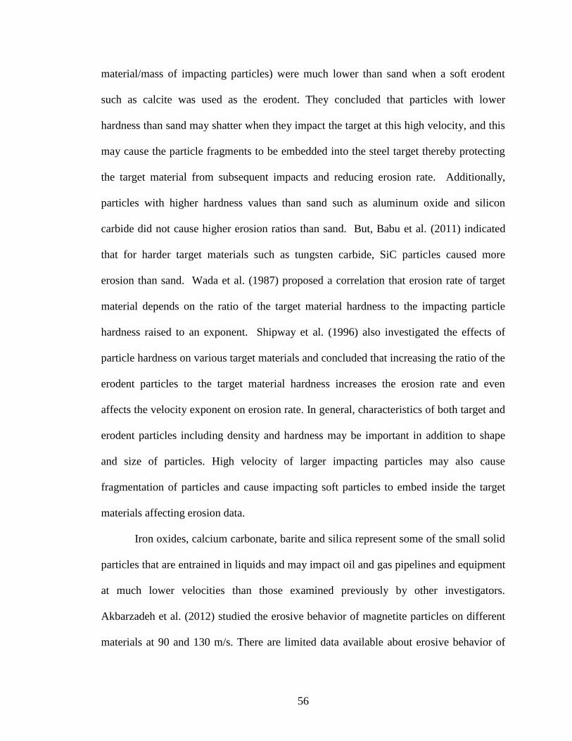
56

material/mass of impacting particles) were much lower than sand when a soft erodent

such as calcite was used as the erodent. They concluded that particles with lower

hardness than sand may shatter when they impact the target at this high velocity, and this

may cause the particle fragments to be embedded into the steel target thereby protecting

the target material from subsequent impacts and reducing erosion rate. Additionally,

particles with higher hardness values than sand such as aluminum oxide and silicon

carbide did not cause higher erosion ratios than sand. But, Babu et al. (2011) indicated

that for harder target materials such as tungsten carbide, SiC particles caused more

erosion than sand. Wada et al. (1987) proposed a correlation that erosion rate of target

material depends on the ratio of the target material hardness to the impacting particle

hardness raised to an exponent. Shipway et al. (1996) also investigated the effects of

particle hardness on various target materials and concluded that increasing the ratio of the

erodent particles to the target material hardness increases the erosion rate and even

affects the velocity exponent on erosion rate. In general, characteristics of both target and

erodent particles including density and hardness may be important in addition to shape

and size of particles. High velocity of larger impacting particles may also cause

fragmentation of particles and cause impacting soft particles to embed inside the target

materials affecting erosion data.

Iron oxides, calcium carbonate, barite and silica represent some of the small solid

particles that are entrained in liquids and may impact oil and gas pipelines and equipment

at much lower velocities than those examined previously by other investigators.

Akbarzadeh et al. (2012) studied the erosive behavior of magnetite particles on different

materials at 90 and 130 m/s. There are limited data available about erosive behavior of

57

small scale products at lower velocities, especially when they are entrained in the liquid.

As stated earlier, erosion is a function of different parameters including particle

size, shape and hardness and because of the different characteristics (exclusively

hardness) of the new particles, sand erosion models are not applicable to calculate erosion

resulting from these particles.

5.2 Experimental data

In this work, two experimental apparatuses have been used, (1) particles entrained

in submerged liquid jet in a slurry tank and (2) gas testing with liquid droplets containing

particles, and the tests have been conducted with nine erodent particles. The details of

experimental setup is described in Chapter 2. The small erodent particles that have been

selected have a wide range of properties (see Table 5.1). Iron powder is the softest

particle with a hardness of 65 kgf mm-2

using the Vickers scale, and silicon carbide is the

hardest (3000 kgf mm-2

). The average size varies from 2 µm (for magnetite) to 40 µm

(for apatite), and the density range is from 2650 to 7860 kg/m3 for silica flour and iron

powder, respectively. Scanning electron microscope (SEM) images of some of these

particles are shown in Figure 5.1. For some of these particles, the average size was

unknown, and SEM images have been processed to characterize the particle size

distribution. Figures 5.2 to 5.6 show the particle size distributions for iron powder,

calcite, barite, magnetite and silica flour, respectively. Density and size of particles affect

their impact velocity as they move in the liquid layers formed on the target wall by the jet

or droplet impacts. It is required to estimate the impact velocities to find a correlation

58

between the particle hardness and induced erosion. CFD simulations and particle tracking

were used to estimate the average impact velocity for each case, but droplet velocity is

not the same as gas velocity in mist flow testing and was measured by particle image

velocimeter (PIV).

Table 5.1 Erodent particle properties

Particle Density

(kg/m3)

Average

size (µm)

Hardness

(VHN)

Iron powder (Fe) 7860 32 65

Calcite (CaCO3) 2710 6 145

Barite (BaSO4) 4300 38 173

Apatite (Ca5(PO4)3) 3140 40 300

Hematite (Fe2O3) 5260 30 600

Magnetite (Fe3O4) 5170 2 680

Silica Flour (SiO2) 2650 24 1000

Alumina (Al2O3) 3950 20 2000

Silicon Carbide (SiC) 3210 20 3000

59

Alumina Silicon carbide

Iron powder

Silica flour

Barite

Magnetite

Figure 5.1 SEM images of erodent particles

30 µm 30 µm

30 µm 30 µm

30 µm 5 µm

60

Figure 5.2 Iron powder particle size distribution

Figure 5.3 Calcite particle size distribution

0

2

4

6

8

10

12

14

16

Less 5 10 15 20 25 30 35 40 45 50 55 60 More

We

igh

t P

erc

en

t (%

)

Size (µm)

0

2

4

6

8

10

12

14

16

Less 2 3 4 5 6 7 8 9 11 12 More

We

igh

t P

erc

en

t (%

)

Size (µm)

61

Figure 5.4 Barite particle size distribution

Figure 5.5 Magnetite particle size distribution

0

5

10

15

20

25

Less 5 10 15 20 25 30 35 40 45 50 55 60 More

Wei

ght

Pe

rcen

t (%

)

Size (µm)

0

5

10

15

20

25

30

35

40

Less 0.2 0.4 0.6 0.8 1 1.2 1.4 1.6 1.8 2 3

We

igh

t P

erc

en

t (%

)

Size (µm)

62

Figure 5.6 Silica flour particle size distribution

Figure 5.7 shows mass loss of the SS-316 specimens after 72 hours of testing in

both submerged and mist flow configurations. Markers are experimental data points and

solid and dashed-dot lines are the average of three experiments conducted at same

condition to show repeatability of the results. The particle throughput in the two

experimental apparatuses was different, so the mass loss values are converted to erosion

ratio (ratio of mass loss to the mass of particles throughput based on concentration and

liquid rate) and plotted in Figure 5.8. Squares are data points for submerged tests, and

diamonds represents mist flow data. Mass losses of the specimens in the submerged test

were higher than what was observed in the mist flow tests because the liquid flow rate

and particle impingement rate were higher, but the erosion ratio is relatively consistent in

the two experiments for most of the particles as it is normalized by the particles

throughput. It should be noted that particles that are impacting the target are impacting at

0

5

10

15

20

25

Less 5 10 15 20 25 30 35 40 More

We

igh

t P

erc

en

t (%

)

Size (µm)

63

different impact velocities due to differences in density and size as they slip through the

liquid protecting the target, and thereby their velocities are much smaller than the liquid

jet and gas velocities.

Figure 5.7 SS-316 mass loss after 72 hours in submerged and mist flow tests

Silicon Carbide

Alumina

Silica Flour

Magnetite

Hematite Apatite

Barite

Calcite Iron Powder

0.0001

0.001

0.01

0.1

1

10

50 100 200 400 800 1600 3200

Mas

s Lo

ss (

g) a

fte

r 7

2 h

rs

Vickers Hardness (VHN)

Submerged Test

Mist Flow Test

64

Figure 5.8 Erosion ratio of the SS-316 specimens for different particles

In order to correlate erosion with particle properties, particle angularity and

impact velocity must be known. Powers (1953) classified particles into six categories

based on their roundness: very angular, angular, sub-angular, sub-rounded, rounded and

well-rounded as shown in Figure 5.9. Experimental results at the Erosion/Corrosion

Research Center (E/CRC) showed that well rounded particles (glass beads) cause four to

five times less erosion than very angular particles (sharp sand), and this phenomenon has

been observed by other researchers (Desale, et al. 2006; Bahadur, et al. 1990). So,

angularity numbers have been assigned to each category from 0.25 for well rounded up to

1.0 for very angular particles and the other categories take numbers in between. Table 5.2

shows angularity numbers assigned to each particle based on the visual observation under

SEM (Figure 5.1). The angularity factor that has been assigned to the particles in this

study ranges from 0.5 to 1. Angularity factors less than 0.5 are not applicable to these

Silicon Carbide

Alumina Silica Flour

Magnetite

Hematite Apatite

Barite

Calcite

Iron Powder

1.E-09

1.E-08

1.E-07

1.E-06

50 100 200 400 800 1600 3200

Ero

sio

n R

atio

, ER

(kg

/kg)


Submerged test

Mist flow test

65

particles because none of these particles are rounded or well-rounded as observed in the

SEM micrographs. So, the possible error associated with this method will be confined in

the specified range.

Figure 5.9 Classification of the particles according to their shape (Powers 1953)

Figure 5.10 shows surfaces of SS-316 specimens eroded by silica flour, iron

powder, barite and magnetite. The top image is in the center of the impacting area, and

the lower images show the eroded surfaces at 4 mm from the center. At the center,

particles impact the specimen normally and platelets are formed on the surface which

may lead to surface failure after repetitive impacts. At locations far from this point,

particles impact the specimen at grazing angles and craters are formed on the surface in

so called scouring erosion phenomenon. The SEM images did not show any fragments of

particles embedded as the impact velocities of these particles with the SS-316 material

are fairly low as shown below. This was confirmed by using Energy Dispersive X-ray

Spectroscopy (EDX) in the locations that were suspicious to have embedded particles

after the test. It is noted that craters created by silica sand are much deeper than others,

1 0.85 0.7 0.55 0.4 0.25

66

and even tiny magnetite particles create craters that are similar to larger silica sand.

Figure 5.10 SEM micrographs of different locations on SS-316 specimens

eroded with different particles

Silica flour Iron powder Barite Magnetite

Silica flour Iron powder Barite Magnetite

67

5.3 Data Analysis and CFD Simulation

It is well known that the major contributor to erosion is impact velocity of

particles. Thus, significant work was dedicated to estimate the representative impact

velocities of these particles. To estimate impact velocity of particles that were entrained

in the liquid droplets, the velocities of droplets were first measured by PIV. Then for

both submerged and mist flow tests, CFD simulations and particle tracking inside the

liquid droplet or jet were conducted to estimate the impact velocity of particles that

penetrate into the liquid layer formed by droplets or continuous jet impact.

ANSYS Fluent is used to study relative motion of the particles with respect to

liquid when it is spreading out on the wall. The simulation for submerged slurry jet

impact was done with the turbulent Reynolds stress model, and after obtaining the steady-

state flow solution, particles were injected at the nozzle exit and modeled as a discrete

phase (DPM) and traced until they leave the simulation domain. Figure 5.11-a and 5.11-b

show velocity contours and particle traces in the submerged configuration, respectively.

For droplets containing small particles, the simulation is more complex. Transient

multiphase flow with volume of fluid (VOF) model was used to simulate a droplet

moving with an initial velocity measured by PIV toward the wall. The initial particle

location, size and velocity were set through an injection file in Fluent and particles traced

until they leave the simulation domain. It is assumed that the droplet and particles that are

inside the droplet have the same initial velocity, and particles are distributed uniformly in

the droplet. For droplet impact, the simulation was done with a laminar fluid model with

uniform mesh over the 10 mm by 15 mm field and the cell size was 5×10-5

m. A variable

time step was used to keep the Courant number below one. The resulting time step was

68

approximately 1 µs.

Figure 5.11-c shows a sequence of a droplet with particles inside during impact.

The velocity of impacting particles was not constant, and the average value from

simulations for both cases is reported in Table 5-2.

a) b)

c)

Figure 5.11 CFD simulation and particle tracking results, a) velocity contours and

b) particle traces in submerged jet flow and c) sequences of droplet impact with

particles

Nozzle Exit

Specimen

Nozzle

Particle Traces

Droplet Entrained

Particles

69

Table 5.2 Average particle impact velocity and angularity

Particle Angularity

Representative normal

component of impact

velocity in submerged

test (m/s)

Average normal

component of impact

velocity in mist flow

tests (m/s)

Iron powder (Fe) 0.50 3.76 6.86

Calcite (CaCO3) 0.75 1.67 2.66

Barite (BaSO4) 0.70 3.45 6.17

Apatite (Ca5(PO4)3) 0.75 3.16 5.36

Hematite (Fe2O3) 0.75 2.99 3.70

Magnetite (Fe3O4) 0.75 1.62 2.10

Silica Flour (SiO2) 1.00 2.75 3.10

Alumina (Al2O3) 1.00 2.11 3.33

Silicon Carbide (SiC) 1.00 1.97 2.89

5.4 Effect of Particle Hardness on Erosion

Figure 5.12 shows test results for submerged and droplet testing obtained in this

study and Levy’s data in the literature that was gathered using an experimental facility,

procedure and velocities that were much different than the current study and were

obtained for much larger particles entrained in gas streams (Levy 1995). The vertical axis

is erosion ratio divided by the normal impact velocity squared to consider the effect of

particle size and density that affect deceleration of a particle when it enters the viscous

70

layer near the wall and divided by the angularity factor obtained from visual observation

of the particles under SEM. Considering that these data were gathered with three

experimental facilities that were considerably different with particle impact velocities

ranging from 2 to 80 m/s, the normalized data appear to line up well as a function of

Vickers hardness of the particles.

Figure 5.12 Correlation between normalized erosion and particle hardness

The dashed line in Figure 5.12 is passed through the data points for which the

hardness of the particle is less than the hardness of SS-316 (~ 220) and other particles

separately. The overall trend of experimental data shows that erosion increases with

particle hardness, but as observed in Figure 5.7 the hardness effect is remarkable when

the hardness of particle is less than the hardness of target material and erosion ratio does

not increase significantly when the particle hardness is higher than the material hardness

Iron Powder

Calcite Barite

Apatite

Hematite

Magnetite

Silica Flour Alumina

Silicon Carbide

1.E-10

1.E-09

1.E-08

1.E-07

1.E-06

50 100 200 400 800 1600 3200

ER (

Kg/

Kg)

/ V

n2

An

gula

rity


Submerged test

Mist flow test

Levy et al. (80 m/s, 30 deg)

trendline

SS-316

71

and the particle keeps its integrity during impact. The erosivity of the particles depends

on their ability to concentrate force locally on the target (Levy et al. 1983, Shipway et al.

1996). When impacting particles are not as hard as the target material, they may deform

during impact, and their kinetic energy will not be effectively transferred to the target

material.

72

CHAPTER 6

LIQUID DROPLET EROSION MODELING

6.1 Introduction

There are many high productivity gas wells around the globe that can produce

large volumes of gas and condensate but are being choked to prevent erosion and erosion-

corrosion. Pipe walls are subjected to erosion not only by sand particles but also by liquid

droplets, and many oil and gas operators believe that the threshold velocity for sand free

production should be based on liquid impact erosion.

In this study, experimental data and a corresponding method in the literature for

erosion caused by liquid impacts are utilized and their applicability to the oil and gas

industry has been examined. Experimental data that has been obtained for several oilfield

materials and the method developed in this study are used to develop a model to predict

the erosion ratio (ratio of volume loss of material to volume of water impinging) of these

materials for a desired condition. This model has been implemented into a method for

predicting droplet impact velocities to predict erosion caused by liquid impacts and

calculate thickness loss rate of oilfield elbow materials for different conditions.

Two cases that are susceptible to become eroded by liquid impacts are shown in

Figure 6.1. In the case when liquid droplets pass through an orifice or in choke flow,

liquid droplets may hit the wall and cause erosion. In another scenario, for two-phase

flow through an elbow, liquid droplets may hit the pipe wall and cause erosion.

73

Figure 6.1 Two possible cases for liquid droplet impingement erosion

6.2 Experimental Data

In the literature, two major types of experimental methods to evaluate the material

integrity exposed to liquid droplet impacts have been utilized. In the first type, specimens

are mounted on a rotating disk or arm and cut through a liquid jet or liquid droplet stream

(see Figure 6.2-a). In the second type, a liquid jet or droplet stream is accelerated to hit a

fixed specimen as shown in Figure 6.2-b. Experimental results show that there is a

significant difference between the results provided by these two types experiment.

(a) (b)

Figure 6.2 Rotating arm and liquid jet erosion experiment schematics

Some of the experimental studies in the literature are as follows. Thiruvengadam

et al. (1970) used aluminum-1100 and SS-316 with diameter of 3/8th

inch mounted on a

ω

V

V

74

rotating disk cutting through a 1/16th

inch jet of water. In Figure 6.3 the number of

impacts required to initiate erosion is shown on the horizontal axis, whereas the vertical

axis shows the corresponding impact velocity. The circle markers show experimental

values for SS-316, and the threshold velocity is estimated to be 150 ft/s. Triangle markers

show values for aluminum, and the corresponding threshold velocity is found to be 50

ft/s.

Figure 6.3 Effect of impact velocity on liquid impact erosion inception

In another study, Baker et al. (1966) used a 12% Chromium Steel specimen

rotating on a disk, hitting water droplets. As shown in Figure 6.4, the maximum values of

erosion rate for different liquid droplet sizes are obtained versus different impact

velocities. The maximum erosion rate is for the maximum size of droplets, 1050 microns,

and the threshold velocity is found to be 120 m/s (390 ft/s).

Another recent example is the work conducted by Higashi et al. (2009). He used a

specimen mounted on a rotating disk cutting a jet flow. Wastage rate of the pipe is

0

50

100

150

200

250

300

350

1.0E+03 1.0E+04 1.0E+05 1.0E+06 1.0E+07 1.0E+08

Imp

act

Ve

loci

ty (

ft/s

ec)

Number of impacts to inception of erosion

SS-316

Al-1100

75

provided in Figure 6.5. The blue color shows that the wastage rate of the pipe is below 2

mm/year, and the orange color shows that this value is over 2 mm/y. Impingement speed

required to erode pipe over 2 mm/year is plotted for aluminum, brass and stainless steel.

So, the threshold velocity is 30 m/s for Aluminum, 40 m/s for brass and 45 m/s for

stainless steel. This observation is clearly not in agreement with the Baker et al. (1966)

study described above.

Figure 6.4 Maximum erosion rate vs. impact velocity (Baker et al. 1966)

Impact Velocity (ft/s)

Max

imu

m E

rosi

on

Rat

e (

kg/k

g)

76

Figure 6.5 Wastage speed of the pipe (Higashi et al. 2009)

Hattori (2010) measured the maximum depth of erosion for three materials: S15C

or carbon steel, stainless steel 304, and STPA24 which is an alloy steel used for pipes. He

used a fixed specimen configuration and accelerated the water jet toward the specimen.

The maximum depth of erosion was measured during exposure time for carbon steel. The

threshold velocity in which no measurable erosion would take place is 80 m/s for carbon

steel and 120 m/s for stainless steel 304.

The results of the experiments reviewed so far are summarized in Table 6.1. The

experiment could be a paddle wheel type with continuous jet or a droplet stream or a

nozzle jet type. Different materials have been used in these experiments but some of them

are similar. It can be seen that the results provided by these different types of experiments

vary significantly.

77

Table 6.1 Experimental studies in the literature

No. Reference Exp. Type Material

Velocity

Erosion

(m/s) (ft/s)

1 Thiruvengadam

et. al. (1970)

Stream &

Paddle

Wheel

Aluminum 15 50 Threshold

Velocities SS-316 46 150

2 Baker et. al.

(1966)

Droplet

& Paddle

Wheel

H.S.S. 120 390 Threshold

Velocity

3 Higashi et. al.

(2009)

Stream &

Paddle

Wheel

Aluminum 30 98

2 mm/y

(78 mpy) Brass 40 131

SS-304 45 147

4 Hattori (2010)

Nozzle

Jet

S15C 80 260

Threshold

Velocities STPA 24 90 295

SS-304 120 393

A set of proprietary experiments were conducted at the University of Tulsa in

1994 by Professor Shadley (Shadley 1994). The “liquid jet and paddle wheel” erosion

apparatus used a design that conforms to the American Society for Testing and Materials

Standard G73-10 (ASTM 2010). The test specimens were mounted on a rotating paddle

wheel by means of special mounting brackets (Figure 6.2-a). The wheel turns at a

constant rotational speed, and a jet of fluid is directed transverse to the plane of rotation

so that the specimens impact the fluid jet. The angular velocity of the wheel dominates

the impact velocity. The specimens are slightly tilted so that the impact angle is 90o.

Figure 6.6 shows how this angle produces a normal impact of resultant velocity. Nine

materials were evaluated in this program. Mechanical properties and chemical

78

composition of materials tested are shown in Table 6.2 and Table 6.3, respectively.

Figure 6.6 (a) Specimen jet normal incidence, (b) 30o impact angle

Table 6.2 Mechanical properties of tested materials

Alloy UNS no. Tensile strength,

ksi

Yield strength,

ksi

Hardness

Brinell

9Cr-1Mo K90941 95 * 68 * 214 *

CS-1018 G10180 99.5 90 210

13 Cr-A S42000 105.1 61.4 200

13 Cr-H S42000 92.7 76.5 197

SS-316 S31603 85 35 210

Sm25-Cr S31260 130 * 125 * 337 *

2205 duplex S31803 90 * 65 * 293 *

Inc 625 N06625 120 * 60 * 200 *

Inc 825 N08825 96 * 49 * 200 *

* approximate value

(a) (b)

Water Jet Velocity

Relative Velocity Component

Normal Incidence Impact Velocity

Specimen Velocity

Water Jet 30o

Specimen

Specimen Velocity

79

Table 6.3 Chemical composition of tested materials in wt% (balance Fe)

Alloy (UNS no.) C Si Mn Cu Ni Cr Mo

9Cr-1Mo (K90941)

0.1 0.5 0.4 0.0 0.0 9.3 1.0

CS-1018 (G10180) 17.0 0.0 0.8 0.0 0.0 0.0 0.0

13 Cr-A (S42000) 0.2 0.6 0.6 0.0 0.0 13.0 0.0

13 Cr-H (S42000)

SS-316 (S31603) 0.0 0.3 1.0 0.0 12.0 17.0 2.5

Sm25-Cr (S31260) 0.0 0.7 1.0 0.5 6.5 25.0 3.0

2205 duplex (S31803) 0.0 1.0 2.0 0.0 5.5 22.0 3.0

Inc 625 (N06625) 0.1 0.5 0.5 0.0 58.0 21.5 9.0

Inc 825 (N08825) 0.0 0.5 1.0 2.2 42.0 21.5 3.0

Materials were cut into cylindrical specimens approximately 0.75 inches in

diameter and 0.25 inches thick. Actual dimensions varied somewhat depending on the

dimensions of the material from which the specimens were cut. Specimens were

mounted on a wheel as depicted in Figure 6.2, and electrically insulated from any other

conductive parts. The wheel was turned at a constant rotational speed by an A.C.

induction motor. A jet of the test fluid was directed transverse to the plane of rotation so

that as the wheel rotated, the specimens would impact the fluid jet, the higher the wheel

rotation speed, the higher the impact velocity. In some tests, the specimens were aligned

so that the impact angle would be 90°, i.e., normal incidence. This is shown in Figure

6.6-a. At the higher wheel rotation rate used (3510 rpm), the velocity of the specimen as

it impacted the test fluid jet was 167 ft/s (51 m/s). The velocity of the liquid jet was

selected to be a minimum of 34 ft/s (10 m/s). Figure 6.6-a shows how adding these two

velocity vectors gives a resultant impact velocity of 170 ft/s (52 m/s) at an angle of 11.5°.

To produce normal incidence, the specimen was tilted 11.5°. To achieve 30o impact, the

80

specimen was rotated about another axis. Figure 6.6-b shows the 30° impact angle

produced by rotating the specimen. In this figure, the water jet is directed into the plane

of the figure. Two test solutions were used: 1) aerated 3% NaCl brine and 2) aerated tap

water. Two impact speeds were used: 1) 170.0 ft/s (high velocity) and 2) 84.6 ft/s (low

velocity). Two impact angles were used: 1) 90° (normal incidence) and 2) 30°. Four

specimens were tested in each test run except for 1018; the specimens tested in each test

run were mixed, i.e., not all specimens on the wheel at one time were the same material.

The 1018 specimens were all run together because they deteriorated much more rapidly

than the other materials. If a 1018 specimen were run with non-deteriorating materials, it

was feared the wheel could become too unbalanced during a test and destroy the

machine's bearings. High velocity tests were run nominally 72 hours. Low velocity tests

were run 144 hours to approximately achieve the same number of impacts as the high

velocity tests. Specimens of 1018 were only run 16 hours because they deteriorated so

rapidly. Adjustments were made in the graphed data to scale weight losses to 144 hour

test periods.

Weight loss for each test was recorded, and the results were averaged for the tests

where more than one specimen was tested. In order to facilitate direct comparison

between different tests, the weight losses that are shown Figure 6.7 are adjusted to a 144

hour test period by assuming that weight loss rates observed in the testing periods would

have continued to the 144th hour. The tests were repeated with high velocity brine and

water for all materials and with other fluids only for carbon steel 1018. The associated

standard error bars are provided in Figure 6.7. It can be concluded generally from the

chart that brine caused more weight loss than tap water, and 1018 carbon steel had the

81

highest weight loss while Inconel 625 had the lowest.

In the high velocity brine test, the four materials of lowest chromium content were

ranked pretty much as one would expect. However, weight losses in the corrosion

resistant alloys were surprisingly high. In some specimens of these materials, chunks of

material appeared to be broken out of the specimens more in the manner of erosion than

of corrosion. The tests were proceeded with the high velocity tap water test assuming

that corrosion losses should be lower for this test, at least for the 1018 and low-chrome

materials. Figure 6.7 also compares the weight losses between brine tests and tap water

tests for the carbon steel and low-chrome materials. Weight losses for the tap water tests

were significantly lower than for brine tests, especially for the 1018 and 9Cr-lMo

materials. But, weight losses for the tap water tests for some of the corrosion resistant

alloys were higher than weight losses for the brine tests.

Figure 6.7 Adjusted mass loss of the specimens to 144 hrs

0.0

1.0

2.0

3.0

4.0

5.0

6.0

9Cr-1Mo CS-1018 13Cr-A 13Cr-H SS-316 Sm25-Cr 2205duplex

Inc 625 Inc 825

Ad

just

ed

we

igh

ht

loss

(g)

Material

High velocity brine (90 deg)

High velocity tap water (90 deg)

Low velocity brine (90 deg)


82

6.3 Erosion Modeling

The adjusted mass loss is not a good parameter to compare erosion/corrosion

conditions of the samples at different condition because it does not account for the

number of impacts of the fluid jet on the specimen, i.e. the total amount of the liquid that

impinged the surface. The volumetric erosion/corrosion ratio (ECR) is defined as the

ratio of volume loss of the target material to the volume of the impinged jet.

𝐸𝐶𝑅 =Volumetric loss

Impinged liquid volume (6.1)

Figure 6.8 shows ECR of the samples tested with high velocity brine and tap

water versus their chromium contents. As one would expect, the ECR is higher for

materials with lower chromium content than corrosion resistance alloys especially when

brine is used as the jet fluid and the effect of jet fluid was significant. This observation

reinforces the hypothesis that the weight losses for the corrosion resistant materials were

primarily due to erosion and not corrosion.

Figure 6.8 ECR versus chromium content of the samples for brine and tap water

0.0E+00

5.0E-08

1.0E-07

1.5E-07

0 5 10 15 20 25 30

ECR

(m

m3 /

mm

3)

Chromimum content (weight %)


High velocity tap water (90 deg)

83

Figure 6.9 provides results for all nine materials for high velocity and low

velocity brine impacting at 90o. It appears that material degradation for 1018 carbon steel

and low-chrome specimens may be controlled by corrosion or a combination of erosion

and corrosion, whereas for corrosion resistant alloys, erosion is the mechanism of

degradation, and it became negligible when impact velocity was reduced. For the two

13Cr materials, the ECR was reduced by the decrease in impact velocity, and as shown in

Figure 6.8, the ECR value was less for water tests than brine. The reason for high ECR

values for brine in comparison to water is the effect of electrolyte conductivity on

corrosion rate. Oxygen corrosion rate increases by increasing salt concentration up to

about 5% because salt increases the conductivity of the solution. However, increasing salt

concentration more than 5% will reduce the corrosion rate because it will reduce the

solubility of oxygen in water. So, it might be hypothesized that there are significant

corrosion and erosion components in the high velocity tests. In liquid impact erosion, it is

believed that repeated impacts fatigue the metal and produce sub-surface cracks if the

impact velocity exceeds the threshold velocity. When cracks propagate and then intersect,

pieces of the fatigued material fall out.

A higher synergistic effect at higher flow velocities can be also explained by

faster removal of corrosion products from the surface. Iron oxide forms on the surface as

a result of oxygen corrosion. Liquid at higher velocities (i.e. with higher erosivity)

removes the corrosion products from the surface faster and creates an active carbon steel

surface without corrosion products that can be corroded faster in comparison to a carbon

steel surface covered with iron oxide.

84

Figure 6.9 ECR versus chromium content of the samples for brine

For the tests at high velocity but with reduced impact angle to 30o (Figure 6.9),

ECR values for 1018 carbon steel and 9Cr-1Mo were of the order of losses observed for

the high velocity normal incidence test; but for materials of higher chromium content, the

30o test results were much lower than for the 90

o tests. This reveals that materials are

more susceptible to erosion loss for normal incidence liquid impacts than for smaller

angles of incidence. This is an important finding in regard to application to injection

wells where liquid impacts the wall at gradual bends at a small angles of incidence.

For materials with high chromium content, weight loss is controlled by erosion.

The American Society for Testing and Materials Standard (ASTM) G73-10 proposed a

standard method to characterize erosion ratio in different conditions. According to this

standard, the maximum erosion ratio is defined as the ratio of material volume loss to the

volume of impinged liquid.

0.0E+00

5.0E-08

1.0E-07

1.5E-07

2.0E-07

2.5E-07

0 5 10 15 20 25 30

ECR

(m

m3 /

mm

3)

Chromimum content (weight %)


Low velocity brine (90 deg)


85

𝐸𝑅𝐿𝑖 = 𝑅𝑒 = (𝑉𝑙𝑜𝑠𝑠𝑉𝑤𝑎𝑡𝑒𝑟

) (6.2)

Also, the incubation period for the number of specific impacts that initiates

erosion can be obtained by multiplying the volumetric incubation period by the projected

area and then dividing by the volume of a single droplet or jet impinged.

𝑁0 = 𝐻0 (𝐴

𝐵) (6.3)

where H0 is incubation period (volume of liquid impinged per unit area), A is projected

area and B is volume of a single impacting drop or jet.

For jets, 𝐻0 = 𝜋𝑑𝑁0

4

For drops, 𝐻0 = 2𝑑𝑁0

3

In each series of experiments, two major parameters determine the erosion

resistance of a specified material, erosion resistance number (NER)

log(𝑁𝐸𝑅) = [∑(log𝑄𝑒𝑖 + log 𝑆𝑒𝑟𝑖)

𝑘

𝑖=1

] 𝑘⁄ − log𝑄𝑒𝑥 (6.4)

and incubation resistance number (NOR)

log(𝑁𝑂𝑅) = [∑(log 𝑆0𝑟𝑖 − log 𝑡0𝑖)

𝑘

𝑖=1

] 𝑘⁄ − log 𝑡0𝑥 (6.5)

where, Qex is maximum erosion rate for test material x, Qei is maximum erosion rate for

reference material i, t0x is nominal incubation period for test material x, t0i is nominal

incubation period for reference material i, Seri is reference erosion resistance for reference

material I and Sori is reference incubation resistance for reference material i.

The NER parameter shows resistivity of the materials against liquid impingement

86

erosion based on the measured mass loss. If we assume that we have a reference material

where the erosion resistance number and incubation resistance are equal to 1, we can

calculate the erosion resistance number and incubation resistance number for each

material with respect to that reference from these correlations. This technique helps to

normalize the erosion resistance of a specific material with respect to a well-known

material and eliminate some of the effects of the experimental method. The normalized

erosion resistances of several materials that were tested are determined from average

values of erosion ratio in the test and are summarized in Table 6.4. The normalized

erosion resistance of SS-316 has been used as a reference. It is observed from the table

that erosion resistance of Inconel 625 to liquid impact is 5 times greater than the

reference material, but the erosion resistance of 1018 to liquid impact erosion-corrosion

is about 7 times less than SS-316.

Table 6.4 Normalized erosion resistance (NER) for several oilfield materials

Designation Normalized Erosion Resistance

(NER)

SS-316 1.00

9Cr-1M 0.25

1018 0.15

13Cr-a 0.90

13Cr-h 0.64

Sm25-Cr 3.43

2205 1.83

625 5.19

Sm825 0.96

87

It is assumed that we have already passed the incubation period which leads to

more conservative results. But generally by obtaining the NER and NOR from

experimental data, we could now use

log 𝑅𝑒 = 4 8 log 𝑉 − logNER − 16 65 + 0 67 log 𝑑 + 0 57 𝐽 − 0 22𝐾 (6.6)

and

log𝑁0 = −4 9 log 𝑉 + logNOR + 16 40 − 0 40 𝐽 (6.7)

to calculate the maximum erosion ratio and incubation period for each material and

desired condition, where N0 is rationalized incubation period, Re is rationalized maximum

erosion rate, NER is“erosion resistance number” of material, NOR is “incubation

resistance number” of material,V is impact velocity in m/s, d is diameter of drops or jet,

in mm, J is 0 for drops and 1 for jets and K is 0 for flat specimens at normal impact and 1

for curved or cylindrical specimens.

In order to assess the obtained model, some experimental values of erosion ratio

(using a paddle wheel type apparatus) for carbon steel from ASTM STP 474 are

compared to model predictions. The results are shown in Figure 6.10. Experimental

values represented by markers have been compared to the model predictions represented

by dashed lines for four different impact velocities. The vertical axis shows the erosion

ratio, and corresponding impact velocities are shown on the horizontal axis. As it can be

seen, both models agree well with data, and the red dashed line is slightly closer to the

experimental values.

88

Figure 6.10 Erosion ratio vs. impact velocity

In another experiment from literature, Baker et al. (1966) measured erosion ratio

values for chromium steel for a range of droplet sizes (350 µm to 1050 µm). The

specimens were mounted on a rotating disk and impacted with liquid droplets. The

ASTM G73-10 correlation predictions have also been compared to this experimental data

in Figure 6.11. The vertical axis shows volumetric erosion ratios, and the corresponding

impact velocities are shown on the horizontal axis. The model predictions closely match

experimental measurements for large droplets and overpredict the values for smaller

droplets at lower impact velocities.

1.0E-07

1.0E-06

1.0E-05

1.0E-04

10 100 1000

ERLi (

mm

3/m

m3)

Impact Velocity (m/s)

Mild steel (Heymann, ASTMSTP474, 1970)

S15C (Hattori et al. 2010)

1018 CS (ASTM Correlation)

1018 CS (E/CRC Correlation)

89

Figure 6.11 Erosion ratio vs. impact velocity (ASTM correlation and exp. data)

The ASTM correlation predictions are good for large droplets (> 1mm), but it

overpredicts the erosion ratios for small droplets, especially at lower velocities. Low

velocities (less than 100 m/s) are more applicable to the oil and gas industry. So, the

correlation has been modified to obtain better predictions at lower velocities and small

droplet sizes as shown by Eq. (6.8).

𝐸𝑅𝐿𝑖 = 10𝑎 𝑉(10−5𝑑

1 3⁄ ) 𝑑9

𝑁𝐸𝑅 , 𝑎 = 0 57 𝐽 − 0 22 𝐾 − 17 1 (6.8)

In the new correlation, the velocity exponent has been changed from a constant

value of 4.8 to a function of droplet size, and the droplet exponent has been raised from

0.67 to 9 as droplet size is also affecting the velocity exponent. The predictions from the

modified correlation have been compared to experimental data discussed earlier from the

1.E-07

1.E-06

1.E-05

1.E-04

50 100 150 200 250 300 350

ERLi (

m3

/m3

)


1050 µm exp1050 µm correlation920 µm exp920 µm correlation660 µm exp660 µm correlation450 µm exp450 µm correlation350 µm exp350 µm correlation

Droplet Size

90

literature (See Figure 6.10 and Figure 6.12). The ER values are now closer to the

experimental data for low velocity cases as compared to ASTM correlation predictions.

Since the source of data for model development is data gathered at E/CRC while

compared values are from experimental data in the literature, the observed deviation is

reasonable.

Figure 6.12 Erosion ratio vs. impact velocity (modified correlation and exp. data)

Based on the ASTM standard and liquid jet impingement tests, a correlation is

proposed to calculate erosion ratio for liquid impact. But for 1018 carbon steel and 9Cr-

1Mo that are not considered corrosion resistant, corrosion is the dominant mechanism of

material degradation. In corrosive conditions, the effects of impact speed and angle are

not as significant as the effect of chemical composition and oxygen content of the fluid

jet. The weight losses of the samples in high velocity normal incidence tests were of the

1.E-07

1.E-06

1.E-05

1.E-04

50 100 150 200 250 300 350

ERLi (

m3/m

3)


1050 µm exp1050 µm correlation920 µm exp920 µm correlation660 µm exp660 µm correlation450 µm exp450 µm correlation350 µm exp350 µm correlation

Droplet Size

91

same order of weight loss as in the low velocity tests. For these materials, corrosion

models (based on material properties, oxygen concentration, temperature, viscosity,

density, and chemical composition of the fluid) and erosion-corrosion models (based on

synergistic effects of erosion and corrosion) should be applied to estimate the wear rate in

the pipe.

6.4 Application to Pipe Flow and Threshold Erosional Velocity Calculation

This erosion model can be applied to estimate the erosion rate at a given operating

condition or calculate the threshold erosional velocity for a given penetration rate.

Erosion rate is a function of impact velocity, droplet size and the amount of liquid

droplets or solid particles that impinge the wall in the time unit. So in both cases, whether

penetration rate is given and threshold velocity is desired or the other way, it is required

to estimate the liquid droplet/solid particle impact velocity, droplet size and entrainment

fraction. One way for extracting this information is the numerical simulation of

multiphase flow with liquid droplet/solid particle trajectories which requires expertise in

computational fluid dynamics (CFD) with a huge computational cost. The alternative is

to estimate the average value of entrainment fraction and droplet size from multiphase

flow correlations and droplet/particle impact velocity from a stagnation length concept

model which has been shown to be acceptable in erosion modeling (McLaury et al.

2000).

A calculation flowchart is provided in Figure 6.13 to apply the model to pipe flow

and to calculate thickness loss rate. Required inputs are superficial liquid and gas

92

velocities, VSL and VSG, diameter of the pipe, D and NER introduced earlier. Output is

thickness loss rate of the pipe. Entrainment fraction, fE, and droplet diameter can be

calculated from mechanistic models that are presented in the literature. The impact

velocity of the liquid droplets can be calculated from the SPPS (Sand Production Pipe

Saver) program in the same way that impact velocity of a sand particle in elbows and tees

is calculated. But, the model for elbows and tees is applied to droplets entrained in a gas

stream and flowing through stagnation layers before they have an opportunity to impact

the pipe wall. The "stagnation layers" reducing the speed of liquid droplets are the gas

and a possible liquid film that may form at the outer walls of an elbow for certain flow

conditions.

Volume loss of the material is obtained by multiplying erosion ratio (from Eq.

(6.8)) by the total volume of the droplets impinging the pipe wall in a given area that is

assumed to be the projected pipe area. Finally, thickness loss is equal to volumetric loss

divided by projected impact area, Ap.

93

Figure 6.13 Calculation procedure of the penetration rate

due to liquid droplet/solid particle impact

Extensive theoretical and empirical studies have been carried out on the

estimation of entrainment fraction and droplet size in two-phase flow systems. For

horizontal flows, Pan and Hanratty (2002) proposed the following correlation to calculate

entrainment fraction in the pipe.

𝑓𝐸 𝑓𝐸𝑚⁄

1 − 𝑓𝐸 𝑓𝐸𝑚⁄= 9 × 10−8 (

𝐷𝑣𝐺3√𝜌𝐿𝜌𝐺

𝜎)(

𝜌𝐺1−𝑚𝜇𝐺

𝑚

𝑑321+𝑚𝑔𝜌𝐿

)

1/(2−𝑚)

(6.9)

Ishii and Mishima (1989) obtained this correlation,

Multiphase Flow Models

𝑬𝑹𝑳𝒊 = 𝟏𝟎𝒂 𝑽(𝟏𝟎−𝟓𝒅

𝟏 𝟑⁄ ) 𝒅𝟗

𝑵𝑬𝑹

𝑽𝑺𝑳 𝑽𝑺𝑮 𝑫 𝑪𝒑

𝒎𝒎

𝒚𝒓𝒐𝒓

𝒎𝒊𝒍𝒔

𝒚𝒓=𝑬𝑹𝑳𝒊 𝑽𝒐𝒍𝒅𝒓𝒐𝒑𝒔

𝑨𝒑

𝑬𝑹 = 𝑬𝑹𝑪 + 𝑬𝑹𝑫

𝑽 𝒇𝑬 𝒅

Droplet/Particle Equation of Motion

𝒎𝒎

𝒚𝒓𝒐𝒓

𝒎𝒊𝒍𝒔

𝒚𝒓=𝑬𝑹 𝑽𝒐𝒍𝒅𝒓𝒐𝒑𝒔 𝝆𝒍𝒊𝒒 𝑪𝒑

𝑨𝒑 𝝆𝒘𝒂𝒍𝒍

Liquid Droplet Impingement Erosion Solid Particle Impingement Erosion

94

𝑓𝐸 = 𝑡𝑎𝑛ℎ(7 25 × 10−7𝑊𝑒1 25𝑅𝑒𝑆𝐿0 25) (6.10)

in which

𝑊𝑒 =𝜌𝐺𝑣𝑆𝐺

2𝐷

𝜎(𝜌𝐿 − 𝜌𝐺𝜌𝐺

)

13 (6.11)

to estimate entrainment fraction in vertical flows. The average droplet size can be

calculated from the Tatterson et al. (1977) correlation.

(𝜌𝐺𝑣𝐺

2𝑑32𝜎

) (𝑑32𝐷) = 0 0091 (6.12)

The impact velocity of the liquid droplets can be calculated from models for

calculating impact velocity of sand particles in elbows and tees. Studies in the literature

have shown that the liquid film along the outer wall of an elbow is sometimes less than

what forms in a straight pipe. The droplet impact velocity is obtained by applying the

following equation of the motion of a droplet with average size estimated above across

the stagnation length,

𝑚𝑉𝑑𝑑𝑉𝑑𝑑𝑥

= 0 5𝜌𝑓(𝑉𝑓 − 𝑉𝑑)|𝑉𝑓 − 𝑉𝑑|𝐶𝐷𝜋𝑑𝑑

2

4 (6.13)

where m is mass of droplet, Vd is droplet velocity, ρf is fluid density, Vf is fluid velocity,

CD is drag coefficient and dd is droplet diameter.

The drag coefficient is calculated from the following correlation.

𝐶𝐷 =24

𝑅𝑒𝑟+ 0 5 , 𝑅𝑒𝑟 =

𝜌𝑓|𝑉𝑓 − 𝑉𝑑|𝑑𝑑

𝜇𝑓 (6.14)

Droplet velocity is unknown in Eq. (6.14) and will be approximated by a one-

dimensional particle tracking model. According to Shirazi et al. (1995b), a stagnation

95

length of L is assumed to be a region near the wall through which the droplet needs to

penetrate to reach the wall. The stagnation length depends on flow geometry and is

estimated empirically as a function of pipe diameter.

𝐿

𝐿0= 1 35 − 1 32 Tan−1(1 63𝐷−2 96) + 𝐷0 247 , 𝐿0 = 1 06 in for Tee (6.15)

𝐿

𝐿0= 1 00 − 1 27 Tan−1(1 01𝐷−1 89) + 𝐷0 129 , 𝐿0 = 1 18 in for Elbow (6.16)

In the stagnation zone, it assumed that the fluid velocity decrease linearly from V0

to zero at wall as shown in Figure 6.14.

𝑉𝑓 = 𝑉0 [1 −𝑥

𝐿] (6.17)

Figure 6.14 Stagnation length for tee and elbow

After substituting for entrainment fraction, droplet size and impact velocity in the

erosion ratio equation for liquid impact, volumetric loss rate of the material is obtained

by multiplying the erosion ratio (from Eq. (6.8)) by the total volume of the droplets

impinging the pipe wall in a given area that is assumed to be the projected pipe area.

Finally, thickness loss is equal to volumetric loss divided by projected impact area, Ap.

For droplets containing small particles there is an extra step in calculating impact

Stagnation Zone

Tee

Stagnation Zone

Elbow

Droplet

x

= 0 [1 −

]

L

0

96

velocity. After the droplet impacts the wall, the particles need to penetrate through the

liquid layer formed on the wall to impact the wall. ANSYS Fluent is used to study

relative motion of the particles with respect to liquid when it is spreading out on the wall.

It is assumed that the droplet and particle have the same initial velocity, and particles are

distributed uniformly in the droplet. Figure 6.15-a shows a sequence of a droplet with

particles inside during impact. Although particle impact velocity can be estimated from

CFD simulation, it is not feasible to run simulations for each droplet size and velocity.

So, the stagnation length concept can be used again by assuming that the representative

particle is located at the center of the droplet and needs to penetrate through the liquid

stagnation length equal to the radius of the droplet to reach the wall. This simplification is

demonstrated in Figure 6.15-b. The next step is to substitute for wall material hardness,

particle sharpness factor and particle impact velocity to calculate erosion ratio for solid

particles. Finally, the penetration rate is equal to the erosion ratio multiplied by

impinging particle mass divided by the density of wall material and impact projected

area. Compared to liquid impingement erosion, the wall material density appears in the

solid particle erosion calculation because the erosion ratio equation for liquid is mostly

expressed in volumetric loss per volume of impinged liquid (e.g. m3/m

3), but the unit of

the erosion ratio equation for solid particles is mass loss per mass of impinging particles

(e.g. kg/kg).

97

Figure 6.15 Sequence of simulated droplet and particle impingement and

corresponding simplified model

The new calculation procedure can be applied in two ways: calculation of

penetration rate for a given flow condition or calculation of threshold erosional velocity

given allowable penetration rate. The second case will be described to compare the

current model predictions to erosional velocities calculated from the API RP 14E

correlation.

Figure 6.16 shows threshold velocity calculations for erosion caused by droplets

with and without particles using the Sand Pipe Saver Program (SPPS) (Shirazi et al.

2000) developed at the E/CRC presented previously compared to predicted values by the

API RP 14E correlation. These calculations have been carried out for an elbow geometry

in a 4-inch (102 mm) pipe. Calculation for a tee joint and other pipe sizes can be easily

done using the stagnation length correlations. The erosional velocity is assumed to be the

velocity at which the erosion rate is 5 mpy (0.13 mm/yr). In these calculations, a sand

size of approximately 25 microns is used which represents impurities or background sand

Droplet Entrained

Particles

L

Droplet

Representative

Particle

(a)

(b)

98

in the liquid with density of 2650 kg/m3 and production rate of 10 lb/day. The solid line is

the threshold boundary for droplets containing particles which yield 5 mpy (0.13 mm/yr).

It follows the trend of SPPS predictions represented by the dash-dot line which is based

on the semi-empirical particle tracking in single and multiphase flows with the same

particles and behaves very differently than the API RP 14E correlation predictions (dash

line). The API RP 14E does not account for solid particle behavior in liquid. In this

correlation, the only parameter that changes with the presence of solid particles in liquid

is the empirical constant C which is 100 for continuous service and 150 to 200 for solids-

free with suppressed corrosion. The threshold line for pure liquid droplet impact (dash-

double dot line) shows relatively high gas velocities. It is observed in the calculation that

as gas velocity increases, droplet size decreases. Small droplets can hardly pass through

the stagnation zone because of their small inertia followed by low impact velocity and

low induced erosion. So, increase in gas velocity increases droplet initial velocity but

decreases impact velocity. Here, it is assumed that droplet size is not reduced below 30

µm to calculate conservative results to compare with other cases, so the actual erosion

may be even less than what is presented in Figure 6.16.

99

Figure 6.16 Comparison of predicted threshold erosional velocity

In another comparison, variations of erosional velocity versus operating pressure

calculated from the API RP 14E correlation and the method and correlation developed in

this work are plotted in Figure 6.17. A tolerable erosion-corrosion rate of 5 mpy (0.13

mm/yr) is assumed, and the operational flow conditions are back-calculated. For these

comparisons, superficial liquid velocity is assumed to be 0.09 m/s, and mean size of the

droplets is assumed to be 200 µm. The constant size of droplets will result in

conservative values for erosional velocity because in real conditions, droplet size

decreases with increase in gas velocity. Erosional velocity is shown on the vertical axis

and operating pressure on the horizontal axis. The model predicts that for higher gas

pressures that are normally encountered in gas producing wells, the droplets are slowed

as the gas density increases and reduces the droplet impact velocity. Thus, the threshold

velocity for liquid droplet impact erosion and erosion caused by solid particles inside the

100

droplet should increase as the pressure is increased. However, the results indicate that

API RP 14E does not follow the trend predicted by the present model. The erosional

velocity predicted by API RP 14 E decreases with gas pressure because the mixture

density increases and erosional velocity is proportional to the inverse of the square root of

mixture density.

Figure 6.17 Variation of erosional velocity versus operating pressure

The behavior of different materials in erosive conditions has been discussed, but

in corrosive conditions, the material behavior is different. Generally, corrosion is

accelerated by increasing the fluid velocity which intensifies the mass transport rate and

also corrosion product scale removal. Lu (2013) discussed that the dependence of

erosion/corrosion rate on impact velocity is

𝑚𝑚

𝑦𝑟= 𝑐𝑜𝑛𝑠𝑡 𝑉𝛽 (6.18)

in which V is the liquid impact velocity in m/s, and the β value depends on the relative

101

contributions of corrosion and erosion to total loss, and it is 0.8 to 1 when corrosion is the

rate controlling process for liquid impacts and 5 to 8 for liquid droplet impingement in

high speed gas flow. The thickness loss rate for liquid impingement erosion is found to be

𝑚𝑚

𝑦𝑟=𝐸𝑅𝐿𝑖 𝑉𝑆𝐿 𝐴

𝐴𝑝≈ 𝐸𝑅𝐿𝑖 𝑉𝑆𝐿 = 𝐶𝑜𝑛𝑠𝑡

𝑉𝛽 𝑑𝛼

𝑁𝐸𝑅 𝑉𝑆𝐿 (6.18)

where ERLi is erosion ratio due to liquid impact, VSL is superficial liquid velocity, A is the

pipe cross-sectional area, Ap is the projected impact area, V is liquid impact velocity, d is

the droplet diameter and NER is the normalized erosion resistance of the target material

that is obtained from experiments. For high speed liquid droplet impact, the ERLi is a

function of impact velocity and droplet diameter, but at low impact velocities and

especially for low chromium alloys, corrosion rate is much higher than erosion rate. So,

the erosion/corrosion ratio (ECR) does not change significantly with impact velocity (see

Figure 6.9). The thickness loss rate may be estimated from

𝑚𝑚

𝑦𝑟≈ 𝐸𝐶𝑅 𝑉𝑆𝐿 = 𝐶𝑜𝑛𝑠𝑡 𝑉𝑆𝐿 (6.19)

The form of this correlation is consistent with the empirical correlation provided by Lotz

(1990). This model has been used to calculate the threshold velocity for an elbow

geometry (made of stainless steel 316 and carbon steel 1018) in a pipe flow system by

assuming a tolerable erosion-corrosion rate of 0.13 mm/yr (5 mpy) and back-calculating

the operational flow velocity. The results are compared to the API RP 14E correlation in

Figure 6.18. The threshold velocity due to erosion is a function of superficial gas and

liquid velocities which determine the rate of liquid impact and impact velocity

respectively, but in the corrosive condition and at superficial gas velocities more than 50

m/s the flow is annular and droplets are moving at similar speeds as the gas velocity. So,

102

they can remove the corrosion scales from the surface, and the liquid flow rate

determines the wastage rate of the pipe. The corrosion line is based on the tests with tap

water as the ECR value for 1018 carbon steel with brine is so high that the calculated

threshold liquid rate is below the minimum value on this figure.

Figure 6.18 Comparison of predicted threshold erosional velocity

0.0001

0.001

0.01

0.1

1

10 100 1000

VSL

(m

/s)

VSG (m/s)

Stainless steel 316

Carbon steel 1018 (Erosion)

Carbon steel 1018 (Corrosion)

API RP 14E

> 5 mpy

< 5 mpy

> 5 mpy

> 5 mpy

< 5 mpy

safe to operate

not safe

103

CHAPTER 7

SUMMARY AND CONCLUSIONS

A unified erosion equation has been developed based on some of the studies in the

literature to calculate the erosion of various metallic samples. The equation is composed

of two parts, cutting erosion that is related to cutting into the surface target material by

striking particles at grazing impact angles and deformation erosion which is caused by

platelet formation and surface failure as a result of multiple collisions of particles in the

normal direction. The distinction of erosion mechanisms for normal and tilted angle

impacts is supported by SEM images of the sample surface as a rough indented surface is

observed at locations where particles impact the surface normally and long craters are

found at locations where particles hit the target at grazing angles.

The model accounts for the particle shape and size and has been validated with

experimental data from direct impingement testing. The particle velocities in gas have

been measured using particle image velocimeter (PIV), and empirical constants have

been incorporated into the final erosion equation based on the experimental data. It was

concluded from experimental data that velocity exponent may be increased from 2 that is

obtained from the formulation to 2.41. Fair agreement has been observed between the

experimental data and model predictions for various samples at different impact

conditions. It was also found that most of the empirical constants follow a trend and can

be correlated to the mechanical properties of the materials indicating that the equations

are capturing the physics of the problem. Also the effects of particle size on the

104

deformation erosion threshold velocity and particle sharpness on erosion were justified

physically. The new equation can be used in CFD simulations and particle tracking codes

to calculate erosion damage for different geometries and materials.

Erosive behavior of very fine particles (iron powder, calcite, barite, hematite,

magnetite, silica flour, alumina and silicon carbide) entrained in liquid has been studied

in two experimental configurations, submerged and mist flow. Particle concentration was

1% by mass and particles were scanned by SEM to characterize representative size

distribution, shape and angularity. PIV was used to measure the velocity of liquid

droplets containing particles, and CFD simulations were performed to estimate the impact

velocity of particles that are entrained by droplets in air/water mist flow or by the liquid

jet spreading over the wall in the submerged case.

Mass loss of a specimen is measured after 72 hours of nonstop testing and

converted to erosion ratio which is defined as the ratio of mass loss of the specimen to

mass of erodent throughput. The results indicate that the induced erosion (mass loss) of

the target specimen is not only a function of particle hardness, but other parameters such

as particle impact kinetic energy and angularity also contribute. So, the erosion ratio

values obtained from the two test configurations were divided by the estimated particle

impact velocity squared and particle angularity to find the erodent hardness dependency

of the erosion. The hardness effect was found to be remarkable when the hardness of the

particle is less than the hardness of target material, and erosion ratio was found to not

increase significantly when the particle hardness is higher than the material hardness and

the particle keeps its integrity during impact.

105

A calculation guideline has been developed based on experimental results and

simplified particle tracking models in the literature to predict erosion rate and threshold

velocities due to the impingement of liquid droplets with or without small particles

entrained. For liquid droplet erosion, the original ASTM G73-10 erosion ratio equation

has been modified to predict better results especially for small droplets at low impact

velocities which are more applicable to oil and gas industry production and transportation

facilities. The erosion ratio of solid particles is calculated from the erosion equations

available in the literature developed based on direct impingement testing with gas.

Entrainment fraction and droplet size in gas-liquid flow in the pipe are estimated

with correlations in the literature. In order to estimate liquid droplet or solid particle

impact velocity, it is assumed that droplets enter a stagnation zone near the wall in which

the fluid velocity decreases linearly from the main stream velocity to zero. For solid

particles, CFD simulations showed that when a droplet spreads over the wall, particles

penetrate into the liquid film formed by the droplet impact and hit the wall. The

stagnation length concept is used again but this time inside the liquid droplet to estimate

impact velocity of a representative particle located initially at the center of the droplet.

By knowing impact condition, one can calculate the erosion ratio either for droplets or

entrained particles from erosion ratio equations. Penetration rate is calculated from the

amount of liquid droplets or solid particles that impinge the wall multiplied by the

erosion ratio. This procedure is implemented to predict threshold erosional velocity for a

sample case and results are compared to API RP 14E and SPPS predicted values. It was

found that the API correlation under estimated the threshold velocity for liquid

impingement erosion and did not correlate with the limitation imposed by particles

106

entrained in liquid droplets, but SPPS predictions that are calculated from another

mechanistic approach for multiphase flows showed similar trends with results obtained

from this guideline. The comparisons also have been made over a range of operating

pressures (from atmospheric pressure to 10000 psi). The API RP 14E predictions do not

follow the trend of calculated values from the present model; it under-predicts the

threshold velocity especially for high pressures. The erosional velocity in the API

equation changes adversely with the fluid mixture density. In this formula, when pressure

increases the density of the mixture increases that leads to lower erosional velocities, but

in the present model and calculation procedure, as pressure increases, the density of the

gas increases so it can decelerate the droplets (with or without particles) that impact the

pipe wall so erosional velocity increases.

107

CHAPTER 8

RECOMMENDATIONS

Erodent particle properties are very important in the calculation of erosion. So, it

is proposed to investigate the effect of particle size, shape and hardness on the erosion of

other materials than presented here and study the erosion angle dependency on particle

sharpness. The minimum impact angle in these tests was 15 degrees, and this was due to

the limitation in the experimental apparatus. So, it would be interesting to conduct some

experiments at lower impact angles and compare the results with the present study. One

of the main applications of the developed erosion equation would be implementation in

CFD codes (such as Fluent) and other erosion models, and it is recommended to use the

erosion equations in the simulation and compare the results to the experimental data for

different geometries and flow conditions.

A calculation guideline is proposed to estimate the erosion-corrosion caused by

liquid impacts and the application includes but is not limited to production, process, and

transportation facilities in petroleum, power plant and aerospace industries. Liquid impact

erosion-corrosion is of great importance from both economical and safety aspects and in

order to obtain more accurate results it is suggested to investigate the problem further and

study the synergistic effect of erosion-corrosion in different materials and using other

fluids (especially CO2 which is very frequently found in the oil and gas industry).

108

BIBLIOGRAPHY

Akbarzadeh, E., Elsaadawy, E., Sherik, A.M., Spelt, J.K., Papini, M., 2012, “The Solid

Particle Erosion of 12 Metals using Magnetite Erodent,” Wear, Vol. 282, pp. 40-

51.

API, 1991, API Recommended Practice for Design and Installation of Offshore

Production Platform Piping Systems, API RP 14E, American Petroleum Institute,

the 5th Edition. Washington D.C., October.

ASTM Standard G73, 2010, “Standard Test Method for Liquid Impingement Erosion

Using Rotating Apparatus”, ASTM International, West Conshohocken, PA, 2010,

DOI: 10.1520/G0073-10 www.astm.org.

Babu, P.S., Basu, B., Sundararajan G., 2011, “The Influence of Erodent Hardness on the

Erosion Behavior of Detonation Sprayed WC-12Co Coatings,” Wear, Vol. 270,

pp. 903-913.

Bahadur, S., Badruddin, R., 1990, “Erodent Particle Characterization and the Effect of

Particle Size and Shape on Erosion,” Wear, Vol. 138, pp. 189-208.

Baker, D. W. C., Jolliffe, K. H., Pearson, D., 1966, “The Resistance of Materials to

Impact Erosion Damage” Philosophical Transactions of the Royal Society of

London. Series A, Mathematical and Physical Sciences, Vol. 260, pp. 193-203.

Bingley, M.S., O’Flynn, D.J., 2005, “Examination and comparison of various erosive

wear models,” Wear, Vol. 258, pp. 511-525.

Bitter, J.G.A., 1963a, “A study of erosion phenomena part I,” Wear, Vol. 6, pp. 5-21.

http://www.astm.org/

109

Bitter, J.G.A., 1963b, “A study of erosion phenomena: Part II,” Wear, Vol. 6, pp. 169-

190.

Bourgoyne, A., 1989, “Experimental Study of Erosion in Diverter Systems Due to Sand

Production,” Proceedings of SPE/IADC Drilling Conference, New Orleans, LA.

Castle, M. J., Teng, D. T., 1991, “Extending Gas Well Velocity Limits: Problems and

Solutions”. Proceedings of SPE Asia-Pacific Conference, Perth. Australia

Chein, R., Chung, J. N., 1988, “Particle Dynamics in A Gas-Particle Flow over Normal

and Inclined Plates,” Chemical engineering science, Vol. 43, pp. 1621-1636.

Chen, Q., Li., D.Y., 2003, “Computer Simulation of Solid Particle Erosion,” Wear, Vol.

254, pp. 203-210.

Chen, X., 2004, Application of Computational Fluid Dynamics (CFD) to Single-phase

and Multiphase Flow Simulation and Erosion Prediction, Ph.D. Dissertation,

Department of Mechanical Engineering , The University of Tulsa

Chen, X., McLaury, B. S., Shirazi, S. A., 2004, “Application and Experimental

Validation of a Computational Fluid Dynamics (CFD)-Based Erosion Prediction

Model in Elbows and Plugged Tees,” Computers & Fluids, Vol. 33, pp. 1251-

1272.

Clark, H. M., 1992, “The Influence of the Flow Field in Slurry Erosion,” Wear, Vol. 152,

pp. 223-240.

Desale, G.R., Gandhi, B.K., Jain, S.C., 2006, “Effect of Erodent Properties on Erosion

Wear of Ductile Type Materials,” Wear, Vol. 261, pp. 914-921.

Dhar, S., Krajac, T., Ciampini, D., Papini, M., 2005, “Erosion Mechanisms due to Impact

of Single Angular Particles,” Wear, Vol. 258, pp. 567-579.

110

Dosanjh, S., Humphrey, J. A., 1985, “The Influence of Turbulence on Erosion by a

Particle-Laden Fluid Jet,” Wear, Vol. 102, pp. 309-330.

Edwards, J., 2000, Development, Validation and Application of a Three-Dimensional

CFD-Based Erosion Prediction Procedure, Ph.D. Dissertation, Department of

Mechanical Engineering, The University of Tulsa.

ElTobgy, M.S., Ng, E., Elbestawi, M.A., 2005, “Finite Element Modeling of Erosive

Wear,” International Journal of Machine Tools and Manufacture, Vol. 45, pp.

1337-1346.

Feng, Z., Ball, A., 1999, “The Erosion of Four Materials using Seven Erodents - Towards

an Understanding,” Wear, Vol. 233, pp. 674-684.

Finnie, I., 1960, “Erosion of Surfaces by Solid Particles,” Wear, Vol. 3, pp. 87-103.

Finnie, I., McFadden, D. H., 1978, “On the Velocity Dependence of the Erosion of

Ductile Metals by Solid Particles at Low Angles of Incidence,” Wear, Vol. 48,

pp. 181-190.

Finnie, I., Wolak, J., Kabil, Y., 1967, “Erosion of Metals by Solid Particles,” Journal of

Materials, Vol. 2, pp. 682.

Goodwin, J. E., Sage, W., Tilly, G. P., 1969, “Study of Erosion by Solid Particles,”

Proceedings of the Institution of Mechanical Engineers, Vol. 184, pp. 279-292.

Grant, G., Tabakoff, W., 1973, “An Experimental Investigation of the Erosive

Characteristics of 2024 Aluminum Alloy,” University of Cincinnati, Department

of Aerospace Engineering Tech. Rep. No. 73-37.

Harsha, A.P., Bhaskar, D.K., 2008, “Solid Particle Erosion Behavior of Ferrous and Non-

Ferrous Materials and Correlation of Erosion Data with Erosion Models,”

111

Materials & Design, Vol. 29, pp. 1745-1754.

Hattori, S., 2010, “Effect of Impact Velocity and Droplet Size on Liquid Impingement

Erosion,” Proceedings of International Symposium on the Ageing Management &

Maintenance of Nuclear Power Plants, Vol. 58, pp. 71.

Head, W. J., Harr, M. E., 1970, “The Development of a Model to Predict the Erosion of

Materials by Natural Contaminants,” Wear, Vol. 15, pp. 1-46.

Higashi, Y., Narabayashi, T., Shimazu, Y., Tsuji, M., Ohmori, S., Mori, M., Tezuka, K.,

2009, “Study on Pipe Wastage Mechanism by Liquid Droplet Impingement

Erosion,” Proceedings of ICAPP, Vol. 9, pp. 10-14.

Huang, C., Chiovelli, S., Minev, P., Luo, J., Nandakumar, K., 2008, “A Comprehensive

Phenomenological Model for Erosion of Materials in Jet Flow, Powder

Technology, Vol. 187, pp. 273-279.

Humphrey, J. A. C., 1990, “Fundamentals of Fluid Motion in Erosion by Solid Particle

Impact,” International Journal of Heat and Fluid Flow, Vol. 11, pp. 170-195.

Hutchings, I.M., 1977, “Deformation of Metal Surfaces by the Oblique Impact of Square

Plates,” International Journal of Mechanical Sciences, Vol. 19, pp. 45-52.

Hutchings, I.M., 1981, “A Model for the Erosion of Metals by Spherical Particles at

Normal Incidence,” Wear, Vol. 70, pp. 269-281.

Hutchings, I.M., 1993, “Mechanisms of Wear in Powder Technology: A Review,”

Powder Technology, Vol. 76, pp. 3-13.

Ishii, M., Mishima, K., 1989, “Droplet Entrainment Correlation in Annular Two-Phase

Flow,” International Journal of Heat and Mass Transfer, Vol. 32, pp. 1835-1846.

J. Shadley, 1994, “Erosion-Corrosion Evaluation of Nine Casing Materials for

112

Application to Kick Point in Condensate Water Injection Wells,”

Erosion/Corrosion Research Center Report, Tulsa, OK.

Johnson, R.W. (Ed.), 1998, “Handbook of Fluid Dynamics,” CRC Press, Boca Raton,

Florida

Laitone, J. A., 1979, “Aerodynamic Effects in the Erosion Process,” Wear, Vol. 56, pp.

239-246.

Levin, B.F., Vecchio, K.S., DuPont, J.N., Marder, A.R., 1999, “Modeling Solid-Particle

Erosion of Ductile Alloys,” Metallurgical and Materials Transactions A, Vol. 30,

pp. 1763-1774.

Levy, A.V., 1995, “Solid Particle Erosion and Erosion-Corrosion of Materials,” ASM

International

Levy, A.V., Chik, P., 1983, “The Effects of Erodent Composition and Shape on the

Erosion of Steel,” Wear, Vol. 89, pp. 151-162.

Li, D.Y., Chen, Q., Cook, B., 2011, “A Further Simulation Study on the Dual Role of

Porosity in Solid-Particle Erosion of Materials,” Wear, Vol. 271, pp. 1325-1330.

Liebhard, M., Levy, A., 1991, “The Effect of Erodent Particle Characteristics on the

Erosion of Metals,” Wear 151, Vol. 1991, 381-390.

Lotz, U., 1990, “Velocity Effects in Flow Induced Corrosion,” NACE Corrosion 90,

Paper No 27.

Lu, B., 2013, “Erosion-Corrosion in Oil and Gas Production,” Research and Reviews in

Materials Science and Chemistry, Vol. 2, pp. 19-60.

Mansouri, A., Shirazi, S.A., McLaury, B.S., 2014, “Experimental and Numerical

Investigation of the Effect of Viscosity and Particle Size on the Erosion Damage

113

Caused by Solid Particles,” Proceedings of ASME 2014 4th Joint US-European

Fluids Engineering Division Summer Meeting, Paper no. 21613, Chicago, IL

McLaury, B., Shirazi, S., Shadley, J., Rybicki, E., 1995, “Parameters Affecting Flow

Accelerated Erosion and Erosion-Corrosion,” CORROSION 95, Paper No. 120,

Houston, NACE International

McLaury, B.S., Shirazi, S.A., 2000, “Is API RP 14E Reliable for Predicting an Erosional

Production Velocity when Sand Production is Anticipated?,” Proceedings of

ETCE/OMAE Joint Conference, pp. 14-17.

Meng, H. C., Ludema, K. C., 1995, “Wear Models and Predictive Equations: Their Form

and Content,” Wear, Vol. 181, pp. 443-457.

Misra, A., Finnie, I., 1981, “On the Size Effect in Abrasive and Erosive Wear,” Wear,

Vol. 65, pp. 359-373.

Molinari, J.F., Ortiz, M., 2002, “A Study of Solid-Particle Erosion of Metallic Targets,”

International Journal of Impact Engineering, Vol. 27, pp. 347-358.

Nguyen, A. V., Fletcher, C. A. J., 1999, “Particle Interaction with the Wall Surface in

Two-Phase Gas-Solid Particle Flow”, International journal of multiphase flow,

Vol. 25, pp. 139-154.

Nidasanametla, S.A., 2012, Effects of Viscosity, Particle Size and Shape on Erosion

Measurements and Predictions, M.Sc. Thesis, Department of Mechanical

Engineering, The University of Tulsa.

Niu, Y. Y., 2001, “Evaluation of Erosion in a Two-Way Coupled Fluid-Particle System,”

International journal for numerical methods in fluids, Vol. 36, pp. 711-742.

Niu, Y.Y., Tsai, C. S., 2000, “Simulation of Erosion by the Dilute Particulate Flow

114

Impact,” Numerical Heat Transfer, Part A, Vol. 37, pp. 167-187.

Njobuenwu, D.O., Fairweather, M., 2012, “Modeling of Pipe Bend Erosion by Dilute

Particle Suspensions,” Computers & Chemical Engineering, Vol. 42, pp. 235-247.

Nokleberg, L., Sontvedt, T. 1995, “Erosion in Choke Valves - Oil and Gas Industry

Applications,” Wear, Vol. 186, pp. 401-412.

Oka, Y.I., Ohnogi, H., Hosokawa, T., Matsumura, M., 1997, “The Impact Angle

Dependence of Erosion Damage Caused by Solid Particle Impact,” Wear, Vol.

203, pp. 573-579.

Oka, Y.I., Okamura, K., Yoshida, T., 2005a, “Practical Estimation of Erosion Damage

Caused by Solid Particle Impact: Part 1: Effects of Impact Parameters on a

Predictive Equation,” Wear, Vol. 259, pp. 95-101.

Oka, Y.I., Yoshida, T., 2005b, “Practical Estimation of Erosion Damage Caused by Solid

Particle Impact: Part 2: Mechanical Properties of Materials Directly Associated

with Erosion Damage,” Wear, Vol. 259, pp. 102-109.

Pan, L., Hanratty, T.J., 2002, “Correlation of Entrainment for Annular Flow in Horizontal

Pipes,” International journal of multiphase flow, Vol. 28, pp. 385-408.

Papini, M., Dhar, S., 2006, “Experimental Verification of a Model of Erosion due to the

Impact of Rigid Single Angular Particles on Fully Plastic Targets,” International

journal of mechanical sciences, Vol. 48, pp. 469-482.

Pereira, G.C., de Souza, F.J., de Moro Martins, D.A., 2014, “Numerical Prediction of the

Erosion Due to Particles in Elbows”, Powder Technology, Vol. 261, pp. 105-117.

Powers, M.C., 1953, “A New Roundness Scale for Sedimentary Particles,” Journal of

Sedimentary Research, Vol. 23

115

Rickerby, D.G., Macmillan, N. H., 1980, “On the Oblique Impact of a Rigid Sphere

against a Rigid-Plastic Solid,” International Journal of Mechanical Sciences, Vol.

22, pp. 491-494.

Salama, M., 2000, “An Alternative to API RP 14E Erosional Velocity Limits for Sand-

Laden Fluids,” Journal of Energy Resources Technology, Vol. 122, pp. 71-77.

Salama, M., Venkatesh, E., 1983, “Evaluation of API RP 14E Erosional Velocity

Limitations for Offshore Gas Wells,” Proceedings of the 15th Offshore

Technology Conference, Houston, TX, Paper No. 4485.

Schuh, M. J., Schuler, C. A., Humphrey, J. A. C., 1989, “Numerical calculation of

particle-laden gas flows past tubes,”, AIChE Journal, Vol. 35, pp. 466-480.

Sheldon, G. L., 1970, “Similarities and differences in the erosion behavior of materials,”

Journal of Fluids Engineering, Vol. 92, pp. 619-626.

Sheldon, G.L., Finnie, I., 1966, “The mechanism of material removal in the erosive

cutting of brittle materials,” J. Manuf. Sci. Eng., Vol. 88, pp. 393-399.

Sheldon, G.L., Kanhere, A., 1972, “An investigation of impingement erosion using single

particles,” Wear, Vol. 21, pp. 195-209.

Shipway, P.H., Hutchings, I.M., 1996, “The Role of Particle Properties in the Erosion of

Brittle Materials” Wear, Vol. 193, 105-113.

Shirazi, S., McLaury, B., 2000, “Erosion modeling of elbows in multiphase flow,”

Proceedings of ASME Fluids Engineering Summer Meeting, pp. 11-15.

Shirazi, S., McLaury, B., Shadley, J., Rybicki, E., 1995a, “Generalization of the API RP

14 E Guideline for Erosive Service,” Journal of Petroleum Technology, August,

pp. 693-698.

116

Shirazi, S., Shadley, J., McLaury, B., Rybicki, E., 1995b, “A Procedure to Predict Solid

Particle Erosion in Elbows and Tees,” Journal of Pressure Vessel Technology,

Vol. 117, pp. 45-52

Simmons, M.J., Hanratty, T.J., 2001, “Droplet Size Measurements in Horizontal Annular

Gas-Liquid Flow,” International journal of multiphase flow, Vol. 27, pp. 861-883.

Springer, G. S., 1976, “Erosion by liquid impact,” John Wiley and Sons, New York, NY

Sundararajan, G., 1991, “A Comprehensive Model for the Solid Particle Erosion of

Ductile Materials,” Wear, Vol. 149, pp. 111-127.

Sundararajan, G., Shewmon, P. G., 1983, “A new model for the erosion of metals at

normal incidence,” Wear, Vol. 84, pp. 237-258.

Svedeman, S. J., 1995, “Experimental Study of the Erosional/Corrosional Velocity

Criterion for Sizing Multiphase Flow Lines, Phase II - Experimental Results,

Final Report” , SwRI Project No. 04-6461, Southwest Research Institute, San

Antonio, Texas

Svedeman, S., Arnold, K., 1993, “Criteria for Sizing Multiphase Flow Lines for

Erosive/Corrosive Service.” SPE Production & Facilities, Vol. 9, pp. 74-80.

Tatterson, D.F., Dallman, J.C., Hanratty, T.J., 1977, “Drop Sizes in Annular Gas-Liquid

Flows,” AIChE Journal, Vol. 23, pp. 68-76.

Taylor, J.R., 1981, “An Introduction To Error Analysis: The Study Of Uncertainties In

Physical Measurements,” University Science Books, Mill Valley, CA

Thiruvengadam, A., Rudy, S. L., 1969, “Experimental and Analytical Investigations on

Multiple Liquid Impact Erosion,” (Washington D.C.: NASA)

Thiruvengadam, A., Rudy, S.L., 1969, “Experimental and Analytical Investigations on

117

Multiple Liquid Impact Erosion,” NASA, Washington D.C..

Tilly, G.P., 1973, “A Two Stage Mechanism of Ductile Erosion,” Wear, Vol. 23, 1973,

pp. 87-96.

Vieira, R.E., 2014, Sand Erosion Model Improvement for Elbows in Gas Production,

Multiphase Annular and Low-Liquid Flow, Ph.D. Dissertation, Department of


Wada, S., Watanabe, N., 1987, “Solid Particle Erosion of Brittle Materials. III. The

Interaction with Material Properties of Target and that of Impingement Particle on

Erosive Wear Mechanism,” J. Ceram. Soc. Jpn., Vol. 95, pp. 573-578.

Wang, Y.F., Yang, Z.G., 2008, “Finite Element Model of Erosive Wear on Ductile and

Brittle Materials,” Wear, Vol. 265, pp. 871-878.

Williams, J. H., Lau, E. K., 1974, “Solid particle erosion of graphite-epoxy composites,”

Wear, Vol. 29, pp. 219-230.

Wong, C.Y., Solnordal, C., Swallow, A., Wu, J., 2013, “Experimental and Computational

Modelling of Solid Particle Erosion in a Pipe Annular Cavity,” Wear, Vol. 303,

pp. 109-129.

Zhang, Y., 2006, Application and Improvement of Computational Fluid Dynamics (CFD)

in Solid Particle Erosion Modeling, Ph.D. Dissertation, Department of


Zhang, Y., Reuterfors, E.P., McLaury, B. S., Shirazi, S. A., Rybicki, E. F., 2007,

“Comparison of Computed and Measured Particle Velocities and Erosion in

Water and Air Flows,” Wear, Vol. 263, pp. 330-338.

118

APPENDIX A

SAND EROSION DATA

Table A.1 Erosion data for carbon steel 1018 at particle velocity of 9.2 m/s

Specimen: Carbon Steel 1018 Gas Velocity: 29.2 m/s

Particle: Sand 150 µm Particle Velocity: 9.2 m/s

Impact Angle

(degree) Specimen # start (g) 600 g 1200 g 1800 g ER (g/g)

90 15 94.8489 94.8485 94.8482 94.8479 5.00E-07

75 15 94.8502 94.8497 94.8495 94.8489 6.67E-07

60 15 94.8519 94.8514 94.8509 94.8502 1.00E-06

45 15 94.8577 94.8567 94.8561 94.8553 1.17E-06

45 15 94.8542 94.8535 94.8527 94.8519 1.33E-06

start (g) 300 g 600 g 900 g

30 53 94.8327 94.8324 94.8321 94.8316 1.33E-06

30 53 94.8311 94.8307 94.8302 94.8297 1.67E-06

30 18 94.8573 94.8566 94.8557 94.8548 3.00E-06

15 20 95.0253 95.0241 95.0232 95.0224 2.83E-06

15 20 95.0224 95.0211 95.0204 95.0196 2.50E-06

119




Impact Angle


90 97 95.0004 94.9997 94.9989 94.9975 3.67E-06

90 22 94.9785 94.9780 94.9773 94.9761 3.17E-06

75 22 94.9767 94.9752 94.9740 94.9733 3.17E-06

75 22 94.9733 94.9712 94.9697 94.9682 5.00E-06

60 24 95.0322 95.0306 95.0281 95.0259 7.83E-06

60 24 95.0259 95.0236 95.0214 95.0181 9.17E-06

45 24 95.0175 95.0155 95.0126 95.0105 8.33E-06

45 24 95.0105 95.0082 95.0057 95.0034 8.00E-06

45 19 94.6094 94.6067 94.6032 94.6007 1.00E-05

30 19 94.6208 94.6176 94.6135 94.6094 1.37E-05

30 57 94.0408 94.0377 94.0335 94.0305 1.20E-05

15 19 94.6559 94.6529 94.6497 94.6464 1.08E-05

15 19 94.6464 94.6432 94.6401 94.6368 1.07E-05

120




Impact Angle


90 22 94.9679 94.9659 94.9632 94.9608 8.50E-06

90 22 94.9608 94.9577 94.9552 94.9527 8.33E-06

75 16 95.0473 95.0440 95.0400 95.0353 6.74E-07

75 97 95.0353 95.0320 95.0271 95.0225 2.89E-07

60 16 95.0654 95.0592 95.0528 95.0470 5.77E-07

60 17 94.9704 94.9644 94.9581 94.9525 6.74E-07

45 97 95.0223 95.0149 95.0077 95.0006 9.62E-08

45 57 94.0806 94.0737 94.0665 94.0585 7.70E-07

30 19 94.6860 94.6759 94.6658 94.6561 3.85E-07

30 18 94.9215 94.9120 94.9016 94.8923 1.06E-06

15 21 94.5256 94.5169 94.5086 94.5010 6.74E-07

15 20 95.0915 95.0832 95.0746 95.0667 6.74E-07

121




Impact Angle

(degree)

Specimen

# start (g) 600 g 1200 g 1800 g ER (g/g)

90 29 46.3141 46.3134 46.3130 46.3128 5.00E-07

75 44 45.7830 45.7828 45.7826 45.7822 5.00E-07

60 34 46.4636 46.4628 46.4624 46.4622 5.00E-07

45 25 48.0385 48.0374 48.0363 48.0354 1.67E-06

45 45 46.7798 46.7793 46.7783 46.7774 1.58E-06

start (g) 300 g 600 g 900 g

30 47 48.8089 48.8084 48.8076 48.8066 3.00E-06

30 47 48.8063 48.8060 48.8053 48.8041 3.17E-06

30 47 48.8089 48.8084 48.8076 48.8066 3.17E-06

15 36 48.0853 48.0843 48.0832 48.0824 3.00E-06

15 36 48.0824 48.0817 48.0809 48.0799 3.00E-06

122




Impact Angle


90 44 45.7869 45.7866 45.7859 45.7852 2.33E-06

90 44 45.7852 45.7848 45.7838 45.7828 3.33E-06

75 45 46.7859 46.7846 46.7837 46.7830 2.67E-06

75 45 46.7830 46.7821 46.7810 46.7798 3.83E-06

60 32 45.6674 45.6658 45.6647 45.6630 4.67E-06

60 32 45.6630 45.6616 45.6596 45.6583 5.50E-06

45 25 46.5378 46.5355 46.5331 46.5305 8.33E-06

45 25 46.5305 46.5278 46.5248 46.5211 1.12E-05

45 34 46.4231 46.4202 46.4178 46.4147 9.17E-06

30 33 46.5211 46.5183 46.5153 46.5123 1.00E-05

30 33 46.5123 46.5095 46.5065 46.5034 1.02E-05

30 34 46.4345 46.4309 46.4277 46.4231 1.30E-05

15 31 47.8859 47.8818 47.8775 47.8735 1.38E-05

15 31 47.8735 47.8699 47.8657 47.8615 1.40E-05

15 27 49.6516 49.6476 49.6431 49.6392 1.40E-05

123


Specimen: 4130 Carbon Steel Gas Velocity: 87.6 m/s


Impact Angle

(degree)

Specimen

# start (g) 300 g 600 g 900 g ER (g/g)

90 36 48.0935 48.0926 48.0905 48.0881 7.50E-06

90 29 46.3270 46.3254 46.3219 46.3209 7.50E-06

75 33 46.5508 46.5471 46.5432 46.5401 1.17E-05

75 32 45.7133 45.7099 45.7063 45.7033 1.10E-05

60 29 46.3638 46.3589 46.3538 46.3478 1.85E-05

60 28 45.8265 45.8216 45.8162 45.8107 1.82E-05

45 29 46.3478 46.3411 46.3347 46.3277 2.23E-05

45 27 46.6716 46.6646 46.6581 46.6511 2.25E-05

30 30 46.8064 46.8014 46.7957 46.7872 2.37E-05

30 28 45.8104 45.8028 45.7952 45.7878 2.50E-05

15 26 48.6468 48.6373 48.6287 48.6213 2.67E-05

15 27 49.6980 49.6891 49.6800 49.6722 2.82E-05

124

Table A.7 Erosion data for stainless steel 316 at particle velocity of 9.2 m/s

Specimen: Stainless Steel 316 Gas Velocity: 29.2 m/s


Impact Angle


90 29 45.59913 45.59897 45.5989 45.59883 2.22E-07

75 29 45.59977 45.59960 45.59933 45.59927 5.56E-07

60 28 45.67527 45.67497 45.67483 45.6748 3.33E-07

45 28 45.67617 45.67580 45.67543 45.67527 8.89E-07

30 28 45.67633 45.67623 45.67617 45.67587 6.11E-07

15 28 45.67813 45.67750 45.677 45.67633 1.94E-06

125




Impact Angle


90 11 44.0738 44.073 44.0720 44.0707 3.83E-06

90 11 44.0707 44.0695 44.0679 44.0668 4.50E-06

75 11 44.0664 44.0646 44.0631 44.0609 6.17E-06

75 11 44.0609 44.0593 44.0576 44.0557 6.00E-06

60 11 44.0557 44.0538 44.0513 44.0492 7.67E-06

60 11 44.0492 44.0469 44.0448 44.0427 7.00E-06

45 11 44.0426 44.0409 44.0381 44.0354 9.17E-06

45 11 44.0354 44.0334 44.0310 44.0281 8.83E-06

30 14 43.4089 43.4068 43.4029 43.3996 1.20E-05

30 14 43.3996 43.397 43.3932 43.3896 1.23E-05

15 3 44.1385 44.1346 44.1313 44.1275 1.18E-05

15 22 46.5415 46.5373 46.5335 46.5296 1.28E-05

126




Impact Angle


90 12 43.1735 43.1703 43.1660 43.1617 1.43E-05

90 18 45.5355 45.5327 45.5288 45.5247 1.33E-05

90 15RF 45.2025 45.1965 45.1911 45.1874 1.52E-05

90 15LF 45.1664 45.1633 45.158 45.1535 1.63E-05

75 2 43.1617 43.1582 43.1538 43.1489 1.55E-05

75 18 45.5249 45.5213 45.5168 45.5125 1.47E-05

60 2 43.1489 43.1432 43.1375 43.1310 2.03E-05

60 18 45.5125 45.5079 45.5014 45.4962 1.95E-05

45 2 43.1310 43.1244 43.1173 43.11041 2.33E-05

45 18 45.4932 45.4894 45.4827 45.4748 2.43E-05

30 12 44.8763 44.8686 44.8610 44.8535 2.52E-05

30 12 44.8535 44.8462 44.8389 44.8315 2.45E-05

15 18 44.8535 44.8453 44.8369 44.8290 2.72E-05

15 13 47.152 47.1427 47.1332 47.1274 2.55E-05

127




Impact Angle


90 47 45.2274 45.2271 45.2269 45.2264 5.83E-07

75 38 44.4951 44.4949 44.4945 44.4942 5.83E-07

60 38 44.4964 44.4959 44.4955 44.4951 6.67E-07

45 14 45.1123 45.1117 45.1112 45.1106 9.17E-07

45 47 45.2335 45.2327 45.2318 45.2309 1.50E-06

30 44 45.1164 45.1158 45.1149 45.1135 1.92E-06

start (g) 300 g 600 g 900 g

30 39 45.1192 45.1183 45.1175 45.1168 2.50E-06

30 39 45.1168 45.1161 45.1156 45.1147 2.33E-06

15 46 45.0578 45.0570 45.0561 45.0556 2.33E-06

15 46 45.0556 45.0548 45.0536 45.0526 3.67E-06

128




Impact Angle


90 45 45.2030 45.2023 45.2014 45.2005 3.00E-06

90 37 45.0435 45.0426 45.0419 45.0407 3.17E-06

75 37 45.0374 45.0362 45.0342 45.0310 8.67E-06

60 43 44.6490 44.6481 44.6459 44.6445 6.00E-06

60 42 44.5196 44.5183 44.5167 44.5149 5.67E-06

45 14 45.1294 45.1277 45.1260 45.1242 5.83E-06

45 14 45.1242 45.1229 45.1213 45.1196 5.50E-06

30 42 44.5144 44.5119 44.5098 44.5068 8.50E-06

30 42 44.5068 44.5043 44.5022 44.4997 7.67E-06

30 45 45.1851 45.1825 45.1802 45.1768 9.50E-06

15 44 45.1318 45.1296 45.1275 45.1251 7.50E-06

15 44 45.1251 45.1208 45.1182 45.1161 7.83E-06

15 40 45.6541 45.6519 45.6488 45.6454 1.08E-05

129




Impact Angle


90 47 45.2438 45.2408 45.2410 45.2371 6.17E-06

90 46 45.0280 45.0278 45.0263 45.0256 3.67E-06

75 45 45.2106 45.2083 45.2051 45.2020 1.05E-05

75 44 45.1396 45.1371 45.1337 45.1311 1.00E-05

60 43 44.6836 44.6799 44.6761 44.6732 1.12E-05

60 42 44.5290 44.5262 44.5226 44.5195 1.12E-05

45 37 45.0553 45.0530 45.0461 45.0412 1.97E-05

45 38 44.5109 44.5064 44.5028 44.4970 1.57E-05

30 40 45.6761 45.6680 45.6609 45.6544 2.27E-05

30 41 44.2888 44.2811 44.2734 44.2672 2.32E-05

15 38 44.5326 44.5246 44.5175 44.5110 2.27E-05

15 39 45.1495 45.1426 45.1361 45.1293 2.22E-05

130

Table A.13 Erosion data for 13 chrome duplex at particle velocity of 9.2 m/s

Specimen: 13 Chrome Duplex Gas Velocity: 29.2 m/s


Impact Angle

(degree)

Specimen

# start (g) 600 g 1200 g 1800 g ER (g/g)

90 3 204.6260 204.6255 204.6252 204.6247 6.67E-07

75 3 204.6276 204.6273 204.6268 204.6260 1.08E-06

60 3 204.6295 204.6289 204.6285 204.6276 1.08E-06

45 3 204.6327 204.6320 204.6309 204.6295 2.08E-06

45 25 204.7585 204.7573 204.7563 204.7550 1.92E-06

start (g) 300 g 600 g 900 g

30 10 204.2932 204.2928 204.2918 204.2911 2.83E-06

30 10 204.2911 204.2906 204.2900 204.2894 2.00E-06

30 5 196.4602 196.4596 196.4588 196.4578 3.00E-06

15 6 203.7730 203.7721 203.7716 203.7711 1.67E-06

15 5 196.5289 196.5281 196.5273 196.5267 2.33E-06

15 5 196.4636 196.4631 196.4618 196.4602 4.83E-06

131




Impact Angle

(degree)

Specimen

# start (g) 300 g 600 g 900 g ER (g/g)

90 12 204.4440 204.4438 204.4428 204.4419 3.17E-06

90 12 204.4419 204.4409 204.4400 204.4390 3.17E-06

75 12 204.4390 204.4384 204.4373 204.4357 4.50E-06

75 12 204.4356 204.4341 204.4330 204.4319 3.67E-06

60 6 203.7253 203.7238 203.7216 203.7198 6.67E-06

45 6 203.7184 203.7176 203.7158 203.7140 6.00E-06

45 6 203.7140 203.7129 203.7112 203.7093 6.00E-06

30 4 201.1053 201.1036 201.1003 201.0978 9.67E-06

30 4 201.0978 201.0959 201.0937 201.0914 7.50E-06

15 4 201.0912 201.0884 201.0858 201.0835 8.17E-06

15 4 201.0835 201.0811 201.0788 201.0762 8.17E-06

15 3 204.6239 204.6210 204.6186 204.6158 8.67E-06

132




Impact Angle

(degree)

Specimen

# start (g) 300 g 600 g 900 g ER (g/g)

90 12 204.4511 204.4488 204.4459 204.4442 7.67E-06

90 11 204.0450 204.0433 204.0412 204.0388 7.50E-06

90 11 204.0388 204.0372 204.0352 204.0327 7.50E-06

75 9 203.0771 203.0745 203.0720 203.0694 8.50E-06

75 9 203.0689 203.0661 203.0630 203.0595 1.10E-05

60 10 204.3166 204.3126 204.3089 204.3049 1.28E-05

60 10 204.3049 204.3012 204.2976 204.2938 1.23E-05

45 88 203.0591 203.0549 203.0495 203.0443 1.77E-05

45 11 204.0621 204.0569 204.0523 204.0462 1.78E-05

30 7 204.7808 204.7752 204.7677 204.7610 2.37E-05

30 8 204.4381 204.4321 204.4255 204.4183 2.30E-05

15 1 204.2287 204.2227 204.2158 204.2105 2.03E-05

15 2 203.2864 203.2791 203.2728 203.2676 1.92E-05

133

Table A.16 Erosion data for Inconel 625 at particle velocity of 9.2 m/s

Specimen: Inconel 625 Gas Velocity: 29.2 m/s


Impact Angle


90 60 49.8835 49.8833 49.8828 49.8826 5.83E-07

75 60 49.8849 49.8847 49.8842 49.8835 1.00E-06

60 60 49.8870 49.8867 49.8859 49.8849 1.50E-06

45 59 45.7243 45.7238 45.7229 45.7220 1.50E-06

45 59 45.7220 45.7211 45.7202 45.7192 1.58E-06

start (g) 300 g 600 g 900 g

30 82 45.7316 45.7314 45.7307 45.7295 3.17E-06

30 82 45.7295 45.7294 45.7292 45.7283 1.83E-06

30 57 47.8312 47.8294 47.8284 47.8271 3.83E-06

15 63 47.6141 47.6129 47.6119 47.6105 4.00E-06

15 63 47.6105 47.6095 47.6086 47.6075 3.33E-06

15 49 48.1547 48.1525 48.1515 48.1496 4.83E-06

134




Impact Angle


90 58 49.6471 49.6469 49.6458 49.6447 3.67E-06

90 58 49.6447 49.6443 49.6434 49.6424 3.17E-06

75 53 49.0276 49.0268 49.0259 49.0253 2.50E-06

75 53 49.0253 49.0242 49.0230 49.0222 3.33E-06

60 53 49.6304 49.6296 49.6280 49.6264 5.33E-06

60 52 49.8965 49.8956 49.8945 49.8930 4.33E-06

45 63 47.6228 47.6219 47.6202 47.6183 6.00E-06

45 63 47.6183 47.6171 47.6153 47.6137 5.67E-06

45 50 48.6403 48.6388 48.6372 48.6355 5.50E-06

30 55 49.4313 49.4297 49.4278 49.4258 6.50E-06

30 55 49.4258 49.4240 49.4219 49.4195 7.50E-06

30 60 49.8733 49.8713 49.8695 49.8669 7.70E-07

30 50 48.6477 48.6456 48.6437 48.6410 7.67E-06

15 55 49.4195 49.4170 49.4142 49.4117 8.83E-06

15 54 47.3141 47.3114 47.3088 47.3062 8.67E-06

15 50 48.6559 48.6528 48.6501 48.6477 8.50E-06

135




Impact Angle


90 53 49.0099 49.0072 49.0041 49.0009 1.05E-05

75 53 49.0223 49.0184 49.0145 49.0099 1.42E-05

60 56 47.2393 47.2349 47.2301 47.2244 1.75E-05

45 56 47.2586 47.2520 47.2455 47.2393 2.12E-05

30 56 47.2816 47.2742 47.2668 47.2586 2.60E-05

15 56 47.3058 47.2981 47.2899 47.2812 2.82E-05

136

Table A.19 Erosion data for aluminum alloy 6061 at particle velocity of 9.2 m/s

Specimen: Aluminum Alloy 6061 Gas Velocity: 29.2 m/s


Impact Angle


90 68 16.3975 16.3975 16.3975 16.3974 8.33E-08

75 68 16.3977 16.3977 16.3976 16.3975 1.67E-07

60 68 16.3978 16.3978 16.3978 16.3976 1.67E-07

start (g) 300 g 600 g 900 g

30 69 16.5861 16.5858 16.5855 16.5854 6.67E-07

30 69 16.5854 16.5852 16.5850 16.5849 5.00E-07

30 57 16.6193 16.6189 16.6184 16.6182 1.17E-06

15 67 16.6681 16.6677 16.6668 16.6665 2.00E-06

15 67 16.6665 16.6658 16.6650 16.6642 2.67E-06

15 57 16.6212 16.6208 16.6201 16.6193 2.50E-06

137




Impact Angle


90 64 16.4377 16.4373 16.4365 16.4359 2.33E-06

90 68 16.3998 16.3994 16.3987 16.3981 2.17E-06

90 78 16.5580 16.5575 16.5566 16.5558 2.83E-06

75 66 16.5729 16.5726 16.5723 16.5715 1.83E-06

75 66 16.5715 16.5713 16.5710 16.5704 1.50E-06

60 65 16.5202 16.5193 16.5186 16.5178 2.50E-06

60 62 16.9126 16.9118 16.9111 16.9101 2.83E-06

60 68 16.3110 16.3099 16.3081 16.3067 5.33E-06

45 64 16.4357 16.4344 16.4324 16.4297 7.83E-06

45 64 16.4297 16.4288 16.4274 16.4259 4.83E-06

45 65 16.5175 16.5159 16.5140 16.5119 6.67E-06

30 61 16.2569 16.2555 16.2532 16.2506 8.17E-06

30 61 16.2506 16.2489 16.2459 16.2437 8.67E-06

15 67 16.6839 16.6819 16.6788 16.6758 1.02E-05

15 67 16.6758 16.6739 16.6713 16.6684 9.17E-06

138




Impact Angle


90 66 16.5695 16.5684 16.5664 16.5640 7.33E-06

90 66 16.5640 16.5628 16.5609 16.5582 7.67E-06

90 64 16.3845 16.3819 16.3799 16.3778 6.83E-06

75 67 16.7052 16.7037 16.7018 16.6998 6.50E-06

75 66 16.5821 16.5805 16.5787 16.5774 5.17E-06

75 64 16.3923 16.3899 16.3875 16.3845 9.00E-06

60 64 16.4465 16.4437 16.4416 16.4379 9.67E-06

60 65 16.5611 16.5586 16.5560 16.5528 9.67E-06

60 64 16.4043 16.4001 16.3962 16.3923 1.30E-05

45 69 16.6009 16.5969 16.5917 16.5859 1.83E-05

45 67 16.7002 16.6963 16.6902 16.6843 2.00E-05

30 65 16.5525 16.5477 16.5418 16.5358 1.98E-05

30 65 16.5358 16.5309 16.5251 16.5196 1.88E-05

15 61 16.2838 16.2771 16.2698 16.2628 2.38E-05

15 69 16.6218 16.6147 16.6076 16.6010 2.28E-05

139

APPENDIX B

EROSION DATA FOR OTHER SOLID PARTICLES

Table B.1 Erosion data for other solid particles in submerged configuration (particle concentration: 1% (kg/kg))

Test Spec. # Liq. Vel.

(m/s) Particle

Time

(hr)

Start

W. (g)

Stop

W. (g) Loss (g) ER (g/g)

submerged 61 16.8 Silicon Carbide 72 45.3887 45.0062 0.3825 2.07E-07



submerged 42 16.8 Alumina 72 45.7791 45.5514 0.2277 1.23E-07



submerged 2 16.8 Silica Flour 72 45.4643 44.6531 0.8112 4.38E-07

submerged 9-R 16.8 Silica Flour 72 47.1676 46.221 0.9466 5.11E-07

submerged 15 16.8 Silica Flour 72 45.4635 44.5647 0.8988 4.85E-07

submerged 6 16.8 Magnetite 72 48.9442 48.8238 0.1204 6.50E-08

140

submerged 11-R 16.8 Magnetite 72 47.3183 47.2012 0.1171 6.32E-08

submerged 33 16.8 Magnetite 72 45.6473 45.5419 0.1054 5.69E-08

submerged 67 16.8 Hematite 72 45.6763 45.0515 0.6248 3.37E-07




submerged 81 16.8 Apatite 72 45.3925 44.2105 1.1820 6.38E-07



submerged 9 16.8 Barite 72 47.3157 47.1903 0.1254 6.77E-08

submerged 5-R 16.8 Barite 72 48.7833 48.6723 0.1110 5.99E-08



submerged 14 16.8 Calcite 72 45.7177 45.7054 0.0123 6.64E-09



submerged 10 16.8 Iron Powder 72 47.1893 47.1699 0.0194 1.05E-08

submerged 6-R 16.8 Iron Powder 72 48.6423 48.6179 0.0244 1.32E-08

submerged 30 16.8 Iron Powder 72 45.6949 45.6709 0.0240 1.30E-08

141

Table B.2 Erosion data for other solid particles in mist flow configuration (particle concentration: 1% (kg/kg))

Test Spec. # Gas Vel.

(m/s)

Liq. Rate

(ml/min) Particle

Time

(hr)

Start

W.(g)

Stop

W. (g) Loss (g) ER (g)

air/water 59 45 800 Silicon Carbide 72 45.4137 45.4093 0.0044 2.69E-07



air/water 34 45 800 Alumina 72 45.5421 45.5375 0.0046 2.81E-07



air/water 3 45 800 Silica Flour 72 48.1979 48.1833 0.0146 8.93E-07

air/water 7-L 45 800 Silica Flour 72 47.3366 47.3282 0.0084 5.14E-07

air/water 17 45 800 Silica Flour 72 45.6758 45.6719 0.0039 2.38E-07

air/water 10-2 45 800 Magnetite 72 47.1699 47.1676 0.0023 1.41E-07

air/water 35 45 800 Magnetite 72 45.4722 45.4717 0.0005 3.06E-08

air/water 45 45 800 Magnetite 72 45.8124 45.8085 0.0039 2.38E-07

air/water 69 45 800 Hematite 72 45.8531 45.8513 0.0018 1.10E-07



air/water 79 45 800 Apatite 72 45.3999 45.3956 0.0043 2.63E-07

142



air/water 7 45 800 Barite 72 47.3402 47.3375 0.0027 1.65E-07



air/water 23 45 800 Calcite 72 45.7687 45.7672 0.0015 9.17E-08



air/water 8 45 800 Iron Powder 60 47.3371 47.3366 0.0005 3.67E-08



143

APPENDIX C

LIQUID IMPACT EROSION DATA

Table C.1 Liquid impact erosion data with brine (high velocity)

# Material Impact vel. (ft/s) rpm Time (hr) Start weight (g) End weight (g) Loss (g)

1 Sm825 173.8 3510 71 11.32244 11.143695 0.178745

1 625 173.8 3510 71 12.358215 12.253387 0.104828

1 2205 173.8 3510 71 11.07646 11.030214 0.046246

1 Sm25-Cr 173.8 3510 71 10.418965 10.400229 0.018736

2 1018 173.8 3510 16 15.096604 14.582415 0.514189

2 1018 173.8 3510 16 14.788804 14.295345 0.493459

2 1018 173.8 3510 16 15.07943 14.579 0.50043

2 1018 173.8 3510 16 15.17995 14.680995 0.498955

3 316 173.8 3510 72 11.51495 11.514325 0.000625

3 2205 173.8 3510 72 10.59611 10.578245 0.017865

3 Sm25-Cr 173.8 3510 72 11.013405 11.009665 0.00374

3 13Cr-A 173.8 3510 72 12.98423 12.95477 0.02946

4 316 173.8 3510 72 11.18814 10.933445 0.254695

144

4 Sm825 173.8 3510 72 12.2282 11.8924 0.3358

4 625 173.8 3510 72 12.619215 12.542455 0.07676

4 13Cr-A 173.8 3510 72 12.911585 12.43835 0.473235

5 Sm825 173.8 3510 72 10.317765 9.99769 0.320075

5 625 173.8 3510 72 11.58382 11.548695 0.035125

5 2205 173.8 3510 72 10.09267 9.920665 0.172005

5 Sm25-Cr 173.8 3510 72 11.09197 10.983735 0.108235

6 316 173.8 3510 44 15.402755 15.278675 0.12408

6 9Cr-1M 173.8 3510 44 16.585615 15.703835 0.88178

6 13Cr-H 173.8 3510 44 13.593535 13.261185 0.33235

6 9Cr-1M 173.8 3510 44 18.209055 17.313155 0.8959

7 316 173.8 3510 72 10.894955 10.603075 0.29188

7 625 173.8 3510 72 12.694465 12.693275 0.00119

7 2205 173.8 3510 72 14.960055 14.78058 0.179475

7 Sm25-Cr 173.8 3510 72 14.843875 14.75773 0.086145

145

Table C.2 Liquid impact erosion data with tap water (high velocity)

# Material Impact vel. (ft/s) rpm Time (hr) Start weight (g) End weight (g) Loss (g)

8 1018 173.8 3510 16 14.084425 13.928385 0.15604

8 1018 173.8 3510 16 14.44622 14.31093 0.13529

8 1018 173.8 3510 16 13.9626 13.798825 0.163775

8 1018 173.8 3510 16 13.85728 13.70532 0.15196

9 316 173.8 3510 72 14.816415 14.472285 0.34413

9 625 173.8 3510 72 13.43372 13.430575 0.003145

9 2205 173.8 3510 72 16.47961 16.311275 0.168335

9 Sm25-Cr 173.8 3510 72 14.09982 14.006315 0.093505

10A Sm825 173.8 3510 69 13.319785 13.241335 0.07845

10A 9Cr-1M 173.8 3510 69 17.77244 17.599755 0.172685

10A 13Cr-A 173.8 3510 69 13.252485 13.149465 0.10302

10A 13Cr-H 173.8 3510 69 13.298375 13.11224 0.186135

10B Sm825 173.8 3510 72 12.503675 12.285425 0.21825

10B 9Cr-1M 173.8 3510 72 13.792735 13.53403 0.258705

10B 13Cr-A 173.8 3510 72 13.513775 13.206925 0.30685

10B 13Cr-H 173.8 3510 72 12.99572 12.76823 0.22749

146

Table C.3 Liquid impact erosion data with brine (low velocity)

# Material Impact vel.

(ft/s) rpm Time (hr)

Start weight

(g) End weight (g) Loss (g)

11-A 1018 87.1 1782 72 14.965355 13.206865 1.75849

11-A 1018 87.1 1782 72 14.68792 12.714295 1.973625

11-A 1018 87.1 1782 72 14.02146 12.249635 1.771825

11-A 1018 87.1 1782 72 14.149435 12.464185 1.68525

12 316 87.1 1782 144 14.767355 14.767305 5E-05

12 625 87.1 1782 144 12.954375 12.9543 7.5E-05

12 2205 87.1 1782 144 16.01646 16.016295 0.000165

12 Sm25-Cr 87.1 1782 144 14.294345 14.293985 0.00036

13 Sm825 87.1 1782 144 13.91797 13.917785 0.000185

13 9Cr-1M 87.1 1782 144 16.163815 14.526175 1.63764

13 13Cr-A 87.1 1782 144 13.236215 13.208375 0.02784

13 13Cr-H 87.1 1782 144 13.184425 13.032385 0.15204

147

Table C.4 Liquid impact erosion data with brine (30 deg impact)

# Material Impact vel.

(ft/s) rpm Time (hr)

Start weight

(g) End weight (g) Loss (g)

14 1018 173.8 3510 16 18.995785 18.44623 0.549555

14 1018 173.8 3510 16 18.92052 18.451505 0.469015

14 1018 173.8 3510 16 18.92364 18.436435 0.487205

14 1018 173.8 3510 16 18.775125 18.303725 0.4714

15 316 173.8 3510 72 15.14194 15.141425 0.000515

15 13Cr-H 173.8 3510 72 13.28482 13.17635 0.10847

15 13Cr-A 173.8 3510 72 13.249035 13.228865 0.02017

15 9Cr-1M 173.8 3510 72 14.903955 14.177575 0.72638

16 Sm25-Cr 173.8 3510 72 17.752385 17.751825 0.00056

16 Sm825 173.8 3510 72 14.37954 14.376535 0.003005

16 625 173.8 3510 72 15.994115 15.990775 0.00334

16 2205 173.8 3510 72 17.93925 17.937895 0.001355

T H E U N I V E R S I T Y O F T U L S A THE GRADUATE ... Dissertations/Hadi... · erosion prediction models such as Computational Fluid Dynamics (CFD) based erosion models and Sand

Documents