T F -D T -D (FDTD) METHOD - Stanford Universitychan/publications/pdf/fdtd96.pdf · The FDTD method 1.1 Maxwell’s equations 1.2 Discretization in space and time 1.3 Time-stepping

FDTD Analysis of Crosstalk Between Striplines

1 of 28

THE FINITE -DIFFERENCE TIME -DOMAIN(FDTD) M ETHOD

Applied to the analysis of crosstalk between parallel striplines

Edward Chan

June 10, 1996

0. Introduction1. The FDTD method

1.1 Maxwell’s equations

1.2 Discretization in space and time

1.3 Time-stepping algorithm

1.4 Boundary conditions

1.5 Sources

1.6 Lumped circuit elements

1.7 Parameter extraction

2. Crosstalk between parallel lossless striplines2.1 Introduction

2.2 Theoretical derivation

2.3 HSPICE transmission line simulation

2.4 FDTD simulation

2.5 Observations

3. Conclusions and future development


2 of 28

0. INTRODUCTION

The impact of interconnects on circuit performance in both the analog and

digital domains is ever increasing. No longer can interconnects be treated as mere

delays or lumped RC networks. Crosstalk, ringing and reflection are just some of

the issues that need to be understood then circumvented or utilized.

The most common simulation model for interconnects is the distributed

RLCG model. Unfortunately, this model has many limitations which can lead to

inaccurate simulations if not used correctly. This report uses the FDTD method to

investigate crosstalk between transmission lines. The actual electromagnetic waves

that propagate along striplines are computed allowing a direct, physical simulation

of the coupling between striplines.

The results are compared to theoretical and HSPICE computations. While all

three computations agree qualitatively, the magnitudes of the crosstalk signals are

quite different. The HSPICE computation is incorrect because the calculated cou-

pling parameters are too large. The FDTD results, on the other hand, are within

25% of theory and can be further improved by using finer discretizations.

The FDTD method produces useful and accurate results in the simple prob-

lem of analyzing crosstalk between parallel coplanar transmission lines. However,

its distinguishing characteristic is its ability to simulate 3-D interconnect structures

or structures exhibiting the skin effect. Since the FDTD method can be parallelized

easily, this method is likely to be used to analyze ever more complex interconnects

on massively parallel computers.

1. THE FDTD M ETHOD

1.1 Maxwell’s equations

The FDTD method solves the time-dependent Maxwell’s equations in one,

two or three-dimensional source-free space. The essential equations are the curl

equations


3 of 28

(1.1.1)

(1.1.2)

where , and . In this work, and

are assumed diagonal which imply that this version of the FDTD method can only

handle linear media. In rectangular coordinates, these curl equations can be written

out component-wise as

(1.1.3)

(1.1.4)

(1.1.5)

and

(1.1.6)

(1.1.7)

. (1.1.8)

The FDTD method solves these curl equations explicitly at each time step.

Maxwell’s divergence equations in source-free media, on the other hand, are implic-

itly obeyed by the formulation of the Yee cell (see section 1.2). It can be shown that

the time derivative of the electric flux emanating from a cell in the FDTD space is

E∇×t∂

∂B–=

H∇×t∂

∂D J+=

B µ[ ]H= D ε[ ]E= J σ[ ]E= µ[ ] ε[ ], σ[ ]

t∂∂Hx 1

µx------

z∂∂Ey

y∂∂Ez–

=

t∂∂Hy 1

µy------

x∂∂Ez

z∂∂Ex–

=

t∂∂Hz 1

µz-----

y∂∂Ex

x∂∂Ey–

=

t∂∂Ex 1

εx-----

y∂∂Hz

z∂∂Hy– σxEx–

=

t∂∂Ey 1

εy-----

z∂∂Hx

x∂∂Hz– σyEy–

=

t∂∂Ez 1

εz----

x∂∂Hy

y∂∂Hx– σzEz–

=


4 of 28

zero, which means that if we begin with zero flux, Gauss’ law in source-free media,

, is satisfied for all time [1]. In the same way, the magnetic divergence

law, , is also satisfied.

1.2 Discretization in space and time

The 3-D FDTD simulation space is made up of cuboidal elements of sides

and known as Yee cells. The six field components, Ex, Ey, Ez, Hx, Hy

and Hz, are defined in each cell as shown in Fig. 1. Note that the field components

are not all located at but laid out in interleaved E-field and H-field

grids. Each E-field component is encircled by 4 H-field components and vice-versa

making the implementation of the curl equations obvious.

The common notation used to describe these fields is, for example

, (1.2.1)

wherex denotes the x-component,n significies that this is the value at the time-step

n, whereas [i,j,k] indexes the Yee cell which contains this particular field. Refering

to Fig. 1, we see that Ex[i,j,k] is actually located at .

It is important to remember that the fields are only defined at points on a grid,

not throughout the entire cell. Intervening values have to be interpolated. The con-

situtive parameters, and , and the conductivity, , can be specified indepen-

dently for each field component, allowing the simulation of linear anisotropic

media. At material boundaries, the weighted average of these material parameters

should be used. Each point can be considered to belong to 8 cuboids as shown in

Fig. 2. Thus the parameter value should be

(1.2.2)

where is the parameter for the surrounding cuboidi. For curved surfaces, the

incorporation of a fuzziness factor in these parameters can lend smoothness to the

otherwise staircase-like construction of objects out of Yee cells.

D∇• 0=

B∇• 0=

∆x ∆y, ∆z

i∆x j∆y k∆z,,( )

Exn

i j k, ,[ ] Ex i12---+

∆x j∆y k∆z,,t n∆t=

=

i12---+

∆x j∆y k∆z,,

ε µ σ

ζ

ζii 1=

8

∑8

---------------=

ζi


5 of 28

Fig. 1: The Yee Cell.

Fig. 2: Each point in the grid belongs to 8 cuboids.

x

y

z

(i,j,k)

Ez

Hz

Hy

Ey

Ex

Hx

∆x

∆z

∆y


6 of 28

Since the fields are only defined at points and each field component is speci-

fied at a different point, the shape of the structure is different for different field com-

ponents. For example, in a 2-D mesh, a square defined for Ey is slightly displaced

from that defined for Ex. Usually this poses no problems if we specify the material

parameters ( , , ) for all the field points enclosed by the object. In Fig. 3, this

requires specifying material parameters at four Ex locations and one Ey location if

we wish to define the lower right square.

Fig. 3: Squares defined for Ex and Ey are displaced.

To obtain explicit update equations for the fields, we need to formulate the

finite-difference approximations to the derivatives. For example, the 2nd-order

accurate central difference approximation of Hx in time is

(1.2.3)

whereas the the approximations in space of the corresponding curl are

(1.2.4)

. (1.2.5)

Note that all three equations approximate the derivatives at time t = n and position

. If we plug these equations into

ε µ σ

y

x

Ey

Ex

t∂∂

Hxn

i j k, ,[ ]Hx

n 1 2⁄+i j k, ,[ ] Hx

n 1 2⁄–i j k, ,[ ]–

∆t------------------------------------------------------------------------------------ O ∆t

2( )+=

z∂∂

Eyn

i j k, ,[ ]Ey

ni j k 1+, ,[ ] Ey

ni j k, ,[ ]–

∆z---------------------------------------------------------------- O ∆z

2( )+=

y∂∂

Ezn

i j k, ,[ ]Ez

ni j 1+ k, ,[ ] Ez

ni j k, ,[ ]–

∆y---------------------------------------------------------------- O ∆y

2( )+=

i∆x j12---+

∆y k12---+

∆z,,


7 of 28

(1.2.6)

we can obtain an explicit update equation for using previous E-

field and H-field components:

.

(1.2.7)

Similar update equations can be obtained for the electric fields.

1.3 Leapfrog time-stepping

As shown in the previous section, H-fields are updated at using

the previous H-field at and E-fields at . E-fields, on the

other hand, are updated at using the previous E-field at and

H-fields at .

Fig. 4: Timeline showing when E and H fields are updated.

To remain numerically stable, the time-step must obey the Courant Stability

Condition

. (1.3.1)

To obtain good spatial resolution, the cell size should be less than a twentieth of the

shortest wavelength

. (1.3.2)

t∂∂Hx 1

µx------

z∂∂Ey

y∂∂Ez–

=

Hxn 1 2⁄+

i j k, ,[ ]

Hxn 1 2⁄+

i j k, ,[ ] ∆tµx------

Eyn

i j k 1+, ,[ ] Eyn

i j k, ,[ ]–

∆z----------------------------------------------------------------

Ezn

i j 1+ k, ,[ ] Ezn

i j k, ,[ ]–

∆y----------------------------------------------------------------–

Hxn 1 2⁄–

i j k, ,[ ]+=

t n12---+

∆t=

t n12---–

∆t= t n∆t=

t n 1+( )∆t= t n∆t=

t n12---+

∆t=

EH EH

n-1/2 n n+1/2 n+1

∆t1

c1

∆x( )2-------------- 1

∆y( )2-------------- 1

∆z( )2--------------+ +

---------------------------------------------------------------≤

∆zλmin

20-----------≤


8 of 28

1.4 Boundary Conditions

The simulation space must be terminated by boundary conditions pertinent to

the problem because the central-difference equations for the E-fields cannot be

applied at the boundary since the curl equation requires H-field values outside the

boundary as shown in Fig. 5. H-fields at the boundary, however, are normal to the

boundary so the curl is well-defined in terms of the tangential E-fields that exist

right at the boundary.

Fig. 5: Fields at the boundary of the simulation mesh.

The three common boundary conditions are the perfect electric conductor

(PEC), perfect magnetic conductor (PMC) and the absorbing boundary condition

(ABC). The PEC simply forces the tangential E-fields to zero, creating a perfectly

reflecting wall (short circuit) for electric fields. The PMC forces the tangential H-

fields to zero at the boundary. Since the tangential fields (Hz) are located half a cell

into the simulation space as shown in Fig. 5, the fields right at the boundary are set

to zero by conceptually placing H-fields of the same magnitude but of opposite sign

half a cell outside the simulation space, forcing the interpolated value at the bound-

ary to zero. The curl is now well-defined in terms of this conceptual H-field and the

H-fields inside the simulation space. This boundary condition forces even symmetry

about the PMC wall.

The third boundary condition attempts to simulate the situation of being in

free space. Waves impinging on the boundaries are absorbed, much as if they sim-

ply kept on propagating without being reflected. The 1-D one-way wave equation

Ex

Hz

Hy

inside

outside

Hz

Hy


9 of 28

(1.4.1)

will completely absorb a wave of the formg(x,y)f(z+vt) traveling in the negative z

direction. However, physical or numerical dispersion will causev to vary with fre-

quency resulting in some reflection. Non-TEM modes, which have velocity of prop-

agation less thanv, will not be well-absorbed either. Fortunately, the homogeneous

stripline supports pure TEM waves which are well-absorb by this boundary condi-

tion. Mur implemented this boundary condition, evaluated at and

, as shown below

.

(1.4.2)

Since not all waves are incident normally on the boundaries, it is necessary to

formulate 3-D one-way wave equations that will absorb oblique-incidence waves.

By factoring the 3-D wave equation

(1.4.3)

and taking the second order Taylor expansion to a square root term, we obtain the

2nd order 3-D one-way wave equation [1]

. (1.4.4)

This boundary condition works quite well as shown in Fig. 8, the example of a

source in the center creating ripples propagating outwards to infinity. No interfer-

z∂∂E 1

v---

t∂∂E

z 0=– 0=

t n12---+

∆t=

z12---∆z=

Eyn 1+

i j 1, ,[ ] Eyn

i j 1, ,[ ]+

2----------------------------------------------------------------

Eyn 1+

i j 0, ,[ ] Eyn

i j 0, ,[ ]+

2----------------------------------------------------------------–

∆z---------------------------------------------------------------------------------------------------------------------------------------

1c---

Eyn 1+

i j 1, ,[ ] Eyn 1+

i j 0, ,[ ]+

2------------------------------------------------------------------------

Eyn

i j 1, ,[ ] Eyn

i j 0, ,[ ]+

2--------------------------------------------------------–

∆t---------------------------------------------------------------------------------------------------------------------------------------

– 0=

x2

2

∂

∂ E

y2

2

∂

∂ E

z2

2

∂

∂ E 1

c2

-----t2

2

∂

∂ E–+ + 0=

z∂t

2

∂∂ E 1

c---

t2

2

∂

∂ E–

c2---

x2

2

∂

∂ E c2---

y2

2

∂

∂ E

z 0=

+ + 0=


10 of 28

ence due to reflected waves is observed. Unfortunately, this boundary condition

fails when used to terminate a stripline. As shown in Fig. 6, this ABC can only be

used in the shaded region. If the ABC is used throughout the entire cross-section, it

will generate longitudinal E-fields creating non-TEM modes and causing reflections

of up to 80%.

Fig. 6: Region where 2nd order boundary conditions can be used.

We investigated possible causes for this behavior but the evidence does not

support any of the possibilities. The impact of evanescent modes is ruled out

because extending the simulated line length, and thus allowing the modes to die out,

does not reduce the reflected wave. Numerical dispersion is not a factor either since

using fourth-order central differencing, which reduces numerical dispersion by two

orders of magnitude, produces no improvements. Neither does using a mesh 4 times

denser along the x and y directions.

When Eq. 1.4.5 is truncated to

(1.4.5)

it becomes equivalent to the first order equation. This truncated boundary condition

works, which implies that the sum of the second derivatives,

, (1.4.6)

should vanish but does not in the region just outside the strip (unshaded in Fig. 6).

1.5 Sources

Three types of sources are commonly used to excite fields in the simulation

space: the wire source, the sheet source and the lumped circuit element source.

Lumped elements are described in the next section.

The wire source, shown in Fig. 7, defines the E-field along a line in the simu-

2nd order ABC’swork only in theshaded region

z∂t

2

∂∂ E 1

c---

t2

2

∂∂ E

z 0=

– 0=

c2---

x2

2

∂∂

Ec2---

y2

2

∂∂

+


11 of 28

lation mesh. Since the value of the field at the source is a fixed function of time,

independent of its surroundings and reflections, it is a hard source and behaves like

a PEC to incident waves. However, the reflections off a thin line are negligible. Fig.

8 shows the fields in the y-z plane emanating from the wire source of Fig. 7. Wire

sources are used to simulate electric probe sources in waveguides.

Fig. 7: Wire source.

Fig. 8: Ex fields in the y-z plane.

However, sheet sources are more commonly used to excite waveguides

because the resulting field pattern settles more quickly to the dominant propagating

mode, thus reducing the required simulation space. The fields exciting a stripline

are shown in Fig. 9. The stripline is fed antisymmetrically above and below the

strip.

x

y

z


12 of 28

Fig. 9: Sheet source.

In this report, the fields in the source have uniform magnitude. If we desire to

establish the dominant mode quickly, we can solve Poisson’s equation, , on

the cross-section then pattern the source fields according to the computed field pat-

tern. This, however, requires two simulation runs.

Since we are also fixing the field values, disregarding the surroundings, we

need to be aware of reflections. We try to keep the source on as long as possible to

allow the excitation, if it is of finite duration, to be generated smoothly. Abrupt ter-

minations generate undesirable higher-order modes. Just before the wave reflected

off the far end returns to the source, we turn on ABC’s at the source to absorb the

reflections.

A more realistic way to excite transmission lines is to use voltage sources,

described in the next section.

1.6 Lumped circuit elements

We can modify the curl equations to include the effect of lumped circuit ele-

ments

. (1.6.1)

For a y-directed element in free space

(1.6.2)

x

yz

far end

source

V∇2 0=

H∇×t∂

∂D JC JL+ +=

JL

I L

∆x∆z-------------=


13 of 28

where IL can be programmed arbitrarily to simulate resistors, capacitors, voltage

sources, inductors, diodes and BJT’s.

Fig. 10: Resistive voltage source.

For example, a resistive voltage source (Fig. 10) obeys Ohm’s Law

. (1.6.3)

In finite-difference form, the equation becomes

. (1.6.4)

A capacitor would obey the equation

. (1.6.5)

In this crosstalk analysis, these lumped circuit elements are used to excite and

terminate the striplines. For better uniformity, the strip is excited by antisymmetric

banks of sources above and below the strip. The resistive loads are also placed

above and below the strips although only one of each is used (Fig. 11).

VS

V

IL

I L

V VS–

RS-----------------=

I L∆yRs------

Eyn 1+

Eyn

+

2---------------------------

Vs

n 1 2⁄+

Rs--------------------–=

I LC∆y∆t

----------- Eyn 1+

Eyn

–( )=


14 of 28

Fig. 11: Lumped element excitation and termination of a stripline.

1.7 Parameter Extraction

We would now like to extract useful circuit parameters from the fields. Fig.

12 shows the dimensions of the cross-section. We excited the stripline using a sheet

source producing a Gaussian pulse: . The bandwidth (between 5%

points) is 22 GHz [2]. We turned on the source for 150 , enough time for the pulse

to be generated completely but not enough for the reflected pulse to arrive back at

the source. We terminated the strip with 1st order ABC’s which give reflections of

less than 0.5%.

Fig: 12: Dimensions of the stripline being analyzed. = 1mm, = 1.925ps, line length = 100

The voltage as a function of time at a given position along z is

(1.7.1)

where the integral is from the ground plane to the strip whereas the current is given

t 50∆t–13∆t

------------------- 2

–exp

∆t

51

26

PEC∆x

∆y

∆x∆y

y

xεr = 1

∆x ∆y ∆z= = ∆t ∆z

V t( ) Ey t( ) yd⋅∫=


15 of 28

by

(1.7.2)

where the integral is a loop around the strip as shown in Fig. 13. Figs. 14 and 15

show the voltage and current waveforms measured at 50 .

Fig. 13: Integration paths for voltage and current.

Fig. 14: V(t) at 50 .

Fig. 15: I(t) at 50 .

We obtain frequency domain information by performing the DFT on the

I t( ) H t( ) ld⋅∫=

∆z

Current

Voltage

∆z

∆z


16 of 28

time-varying waveforms at various frequencies up to 22 GHz (the pulse bandwidth).

The FFT is less suitable because the time step is so small that the resultant fre-

quency range is too wide. The line impedance is defined as

. (1.7.3)

For frequencies up to 22 GHz, the FDTD simulation gives a constant value of

45.7Ω. Table 1 shows line impedances extracted using other methods. This shows

that the FDTD method is fairly accurate, and accuracy can be improved by simply

increasing the density of the mesh at the expense of simulation time as shown by

Becker [3]. Table 2 shows the Gaussian pulse guided by the stripline. The fields are

slightly higher near the edges of the strip.

Table 1: Line Impedance Of Stripline

Method Line Impedance (Ω)

FDTD (this report) 45.7

Becker (1x density) 45.7



MagiCAD 48.9

XFX 48.8

HSPICE 48.3

Z0DFT V t( )[ ]DFT I t( )[ ]----------------------------=


17 of 28

2. CROSSTALK BETWEENTRANSMISSION LINES

2.1 Introduction

In a system consisting of two parallel striplines, shown schematically in Fig.

16, a signal propagating down one line (the active line) will generate a signal on the

adjacent line (the passive line). This is a significant source of noise in digital circuits

and is increasingly severe as signal rise times continue to decrease and routing den-

sities increase.

Fig. 16: Schematic drawing of two transmission lines in parallel.

Table 2: Ey in the x-z plane

t = 100 t = 200 t = 300∆t ∆t ∆t

Active line

Passive lineNear end

Far end

tr

Input step


18 of 28

The most common circuit model of this lossless coupled system is the distrib-

uted LC circuit shown in Fig. 17.

Fig. 17: Distributed LC circuit model of two coupled transmission lines.

CS is the self-capacitance with respect to the ground plane whereas CM is the

mutual capacitance. LS is the self-inductance of the line whereas LM is the coupling

inductance between the two lines. All these parameters are per unit length.

2.2 Theoretical Derivation of Crosstalk Between LooselyCoupled Lossless Transmission Lines

In a system of two identical parallel transmission lines, the Telegrapher’s

Equations can be modified to become [4]

(2.2.1)

(2.2.2)

(2.2.3)

(2.2.4)

LmCm

CS

LS

x∂∂I 1– C

t∂∂V1 Cm t∂

∂V2–=

x∂∂I 2– C– m t∂

∂V1 Ct∂

∂V2+=

x∂∂V1– L

t∂∂I 1 Lm t∂

∂I 2+=

x∂∂V2– Lm t∂

∂I 1 Lt∂

∂I 2+=


19 of 28

C is thetotal capacitance per unit length of the line. This is the C11 term -- the

sum of the self-capacitance and the mutual capacitances -- in the capacitance matrix

generated by field solvers.

Assume loose coupling, then take the Laplace transform to obtain

(2.2.5)

(2.2.6)

(2.2.7)

. (2.2.8)

We can combine the equations to give

(2.2.9)

(2.2.10)

where , and .

The first equation shows that the approximations completely decouple the

active line signal from the passive line. Thus the signal on the active line propagates

freely, as if in isolation. The passive line, described by the second equation, how-

ever, is driven by the active signal. The solution for the passive line when termi-

nated by its characteristic impedance is

.(2.2.11)

At the near end (x = 0), the solution simplifies to

. (2.2.12)

x∂∂I 1– sCV1=

x∂∂I 2– sCV2 sCmV1–=

x∂∂V1– sLI1=

x∂∂V2– sLI2 sLmI 1+=

x

2

∂∂ V1 s2

v2-----V1– 0=

x

2

∂∂ V2 s2

v2-----V2–

s2

v2-----γ k 1–( )V1=

γCM

C--------= k

CM

C-------- L

LM-------⋅= v

1

LC------------=

V2 γ V k 1+( )4

--------------------- es

xv--

–

es

2l x–v

------------- –

– γ V k 1–( )2

--------------------- xv--

sV( )es

xv--

–

–=

V2 γ V k 1+( )4

--------------------- 1 es

2lv-----

–

–=


20 of 28

The first term describes a scaled replica of the input whereas the second term

describes the wave of opposite sign which cancels the initial wave after a delay of

. At the far end (x = l),

(2.2.13)

which predicts that, after a delay of , the scaled derivative of the input waveform

will appear. These results are shown graphically in Table 3 along with results for

other passive line terminations [5].

From the derivations, it is clear that the noise signals depend on the coupling

strength, , which is 13.8 x 10-3 [6] for the stripline dimensions shown in

Fig. 12 and separated by a distance 5∆x. Another parameter, , charac-

terizes the homogeneity of the transmission line. For the homogeneous stripline, k =

1. Other important parameters are wave propagation speed (assuming TEM mode),

v, rise time,tr, and coupling length,l. In the following simulations,v = 3 x 108 ms-1,

tr = 100 ps,l = 60 mm andl/v = 200 ps. Using these values, the predicted wave-

forms are shown in the second column of Table 3. Note that since k = 1, the far end

crosstalk signals are somewhat simplified since the (k-1) terms go to zero.

2lv-----

V2 γ–V k 1–( )

2--------------------- l

v--

sV( )es

lv--

–

=

lv--

γCM

C--------=

kCM

C-------- L

LM-------⋅=


21 of 28

2.3 HSPICE Simulations

The HSPICE simulations used U-model striplines described by ELEV=1

Table 3: Crosstalk between striplines (theoretical)

PassiveLine

Termination

Crosstalk between striplines(theoretical)

Computed Waveform Based onMagiCAD Parameters

Case #1

Case #2

Case #3

γ(k+1)/4

2l/v 2l/v + trtr

near end

γ(k-1)l/2vtr

l/v l/v + tr

far end

6.9 mv

400 500100

200 300

γ(k+1)/2

2l/v

2l/v + tr

tr

γ(k+1)/2

4l/v 4l/v + tr

near end 13.8 mv

400

500

100 800 900

13.8 mv

−γ(k+1)/4

l/v l/v + tr

−γ(k+1)/4 -γ(k-1)l/2vtr

3l/v + tr3l/v

far end

−γ(k-1)l/2vtr 6.9 mv

200 300 700600


22 of 28

(physical) parameters such as width, thickness, height and spacing. Since the ele-

ment parameters (capacitance and inductance) are computed from analytic curve-fit

equations, the parameters have limited ranges of validity. In this report, all the ratios

of dimensions, width to thickness ratio for example, fall within the recommended

ranges [7]. Thus, the errors in coupled line simulations are expected to be less than

15%. However, we found the errors to be much larger.

The gear integration method was used instead of the default trapezoidal

method because it gives less dispersion and ringing when applied to a test simula-

tion of a square pulse propagating down a single 100 cm distortionless stripline. 400

LC elements (lumps) were required to obtain good accuracy, many more than the

default of 20 lumps. Fig. 18 shows the effect of the number of lumps and the meth-

ods of integration on the shape of the output pulse. We see that although the input

pulse is the same for all three cases, the output pulses are quite different. Only the

case with gear integration and 400 lumps exhibits no distortion whereas the other

two cases show ringing and even undershoot. The results shown were obtained

using HSPICE release 95.2 [8]. The latest 96.1 release improves the trapezoidal

integration algorithm, reducing much of the ringing.

The resultant waveforms in the crosstalk simulations, using gear integration

and 50 lumps, are shown in Table 4. The stripline cross-section is as described in

Section 2.2 and shown in Fig. 12. The lines are each 60 mm long. We see that the

waveforms have the expected shape and timing. However, the magnitude of the sig-

nals are about 150% larger than predicted by theory. A reason for this is the discrep-

ancy in coupling parameters between those computed by MagiCAD and those used

by HSPICE. Table 5 compares those critical parameters.


23 of 28

Fig. 18: Square pulse propagating down a distortionless stripline.Rise time = 100 ps, Line length = 100 cm, Step size = 1 ps

Table 4: HSPICE and FDTD computation of crosstalk

Passive LineTermination

HSPICE computation FDTD computation

Case #1

lumps=100

trapezoidal

near end

far end

near end

far end


24 of 28

Case #2

Case #3

Table 5: Distributed LC circuit parameters

Parameter MagiCAD HSPICE % difference

Total capacitance (pF/m) 67.8 69.1 +2.0

Coupling capacitance (pF/m) 0.933 2.42 +159

Self inductance (nH/m) 162 161 -0.6

Mutual inductance (nH/m) 2.20 5.63 +156

Table 4: HSPICE and FDTD computation of crosstalk

Passive LineTermination

HSPICE computation FDTD computation

near end

near end

far endfar end


25 of 28

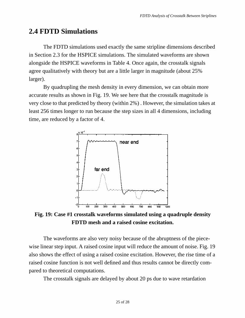
2.4 FDTD Simulations

The FDTD simulations used exactly the same stripline dimensions described

in Section 2.3 for the HSPICE simulations. The simulated waveforms are shown

alongside the HSPICE waveforms in Table 4. Once again, the crosstalk signals

agree qualitatively with theory but are a little larger in magnitude (about 25%

larger).

By quadrupling the mesh density in every dimension, we can obtain more

accurate results as shown in Fig. 19. We see here that the crosstalk magnitude is

very close to that predicted by theory (within 2%) . However, the simulation takes at

least 256 times longer to run because the step sizes in all 4 dimensions, including

time, are reduced by a factor of 4.

Fig. 19: Case #1 crosstalk waveforms simulated using a quadruple densityFDTD mesh and a raised cosine excitation.

The waveforms are also very noisy because of the abruptness of the piece-

wise linear step input. A raised cosine input will reduce the amount of noise. Fig. 19

also shows the effect of using a raised cosine excitation. However, the rise time of a

raised cosine function is not well defined and thus results cannot be directly com-

pared to theoretical computations.

The crosstalk signals are delayed by about 20 ps due to wave retardation

near end

far end


26 of 28

(waves require a finite amount of time to traverse the spacing between lines). This

effect is not captured by the HSPICE simulations. Also, a far end crosstalk signal is

observed even when the passive line is terminated by its charateristic impedance

(Case #1). This is due to an additional fringe capacitance (Fig. 20) of about 16fF at

the near end that disrupts homogeneity and generates separate capacitive and induc-

tive waveforms that do not cancel out at the far end.

Fig. 20: Extra fringing capacitance at the near end.

2.5 Observations

Table 6: Comparison between HSPICE and FDTD

HSPICE FDTD

Good agreement of waveform shapeand timing with theory.

Good agreement of waveform shapeand timing with theory.

Poor agreement in magnitude ofcrosstalk (150% larger than theory)due to incorrect coupling parameters.

Reasonable agreement in magnitude ofcrosstalk (25% larger than theory).Accuracy improves with mesh refine-ment (within 2% with quadruple den-sity mesh).

Can filter input step to prevent unreal-istic ringing.

Difficult to filter input therefore outputis noisy. But can use raised cosine.

2.3 user secs on HP 9000/700 using50 lumps.

17 user secs on HP 9000/700 using sin-gle density mesh. 74 min 52 secs usingquadruple density mesh.

ExtraCapacitance


27 of 28

3. CONCLUSIONS

For most users, HSPICE modeling of crosstalk is fast and adequate (once the

coupling parameters are corrected), except when frequency-dependent effects are

important, coupling is weak or conductors are irregular or 3-D in nature. The FDTD

method distinguishes itself when lumped circuits and distributed circuits are inade-

quate. The challenge is to determine when the extra information provided by the

Easy to set up, modify and inspectresults. Commercial GUI.

Difficult to set up, modify grid orparameters, and inspect results. Cus-tom C program. XFDTD by RemcomInc. is a possibly viable commercialproduct.

No retardation (delay) effect. Crosstalk is retarded (delayed).

No effect of fringing. Fringing capacitance at the near endcauses a pulse at the far end.

Does not model modal dispersioncorrectly (RLCG model cannot han-dle non-TEM modes).

No difficulty with higher-order modes,except that the definition of voltage andcurrent becomes ambiguous.

Two-dimensional (uniform) struc-tures.

Three-dimensional structures. Can han-dle vias, fan out and other discontinui-ties.

All parasitics have to be includedexplicitly.

Models reality.

Can only handle regular systems withratios of dimensions within theallowed range.

Can model any system, even conduc-tors of irregular geometry.

Cannot simulate frequency-depen-dent effects (including skin effect).

Can simulate frequency dependenteffects such as skin effect and complexdielectric loss.

Table 6: Comparison between HSPICE and FDTD

HSPICE FDTD


28 of 28

FDTD method is worth the added complexity and computation cost.

User’s of both the FDTD method and HSPICE need to always be aware of the

limitations of the simulators especially concerning discretization. Finer meshes or

smaller lumps usually improve accuracy at the expense of computation time. How-

ever, HSPICE can suffer convergence problems if too many lumps are used.

The FDTD domain is easily partitioned, making it ideal for parallelization.

Each partition can be computed independently. Boundary values (between parti-

tions) only need to be exchanged at the end of each computation time step. As com-

puting costs decrease, the use of the FDTD method to aid signal integrity

verification will continue to expand.

REFERENCES

[1] A. Taflove, “Computational Electrodynamics,”Artech House, 1995.

[2] X. Zhang and K.K. Mei, “Time-Domain Finite Difference Approach to the Cal-

culation of the Frequency-Dependent Characteristics of Microstrip Disconti-

nuties,”IEEE Trans Microwave Theory and Techniques, vol 36 no 12, Dec

1988, pp 1775-1787.

[3] W.D. Becker, “The Application of Time-Domain Electromagnetic Field Solvers

to Computer Package Analysis and Design,” Ph.D. Thesis, University of Illi-

nois at Urbana-Champaign, 1993.

[4] D.B. Jarvis, “The Effects of Interconnections on High-Speed Logic Circuits,”

IEEE Trans Electronic Computers, Oct 1963, pp 476-487.

[5] J.A. DeFalco, “Reflection and Crosstalk in Logic Circuit Interconnections,”

IEEE Spectrum, Jul 1970, pp 44-50.

[6] MagiCAD 2.1.0, Mayo Foundation, Special Purpose Processor Development

Group.

[7] HSPICE 96.1 User’s Manual, Meta Software, Inc.

[8] HSPICE 95.2, Meta Software, Inc.

T F -D T -D (FDTD) METHOD - Stanford Universitychan/publications/pdf/fdtd96.pdf · The FDTD method 1.1 Maxwell’s equations 1.2 Discretization in space and time 1.3 Time-stepping

Documents