T-61.3010 DSP 2007 (B+C) 1/152 T-61.3010 Digital Signal Processing and Filtering T-61.3010 Digitaalinen signaalink¨ asittely ja suodatus (B) Exercise material for spring 2007 by professor Olli Simula and assistant Jukka Parviainen. Corrections and comments to [email protected], thank you! This material is intended for“paper sessions” on Tuesdays 12-14 L (in English), on Wednesdays 10-12 G, and on Thursdays 14-16 G, in spring 2007. Each problem [Bxx] refers to Problem xx in this material, see p. 2–4. Bring your own copy when coming to the session. The course follows the book “Digital Signal Processing” by Sanjit K. Mitra. There are three different editions available, 3rd being the newest. Notation (Mitra 2Ed Sec. 5.2 / 3Ed Sec. 4.2 ) refers to the section 5.2 in the 2nd Edition (yellow cover) of Mitra’s Book and to the section 4.2 in the 3rd Edition (blue, antenna). There is a brief correspondence table of three editions and errata lists in the course web pages http://www.cis.hut.fi/Opinnot/T-61.3010/. Course lecture slides by Olli Simula follow the third edition of Mitra’s book. This copy belongs to: Contens Description of Example Problems 2 Example Problems 5 Solutions to Example Problems 27 Formula tables 148 T-61.3010 DSP 2007 (B+C) 2/152 Description of Example Problems # Subject Math Background 1-12 1 complex numbers, Carthesian and polar coordinate systems, Euler’s formula 2 Euler’s formula, cosine and sine, odd and even functions 3 complex numbers, graphical notation 4 complex-valued function 5 cosine function, amplitude, frequency, phase 6 logarithm, decibels, sinc, modulo, binary number representation 7 roots of a polynomial 8 complex-valued function, roots of polynomial 9 partial fraction expansion / decomposition 10 sum of geometric series 11 integral transforms 12 matrix product Discrete-time Signals and Systems 13-29 M 2Ed Sec. 2, 3Ed Sec. 2 13 analog, discrete-time and digital signal 14 signals and sequences, unit impulse and unit step functions (δ[n], μ[n]) 15 periodic signals 16 moving average 17 flow / block diagram of a discrete-time system 18 recognition of LTI systems, causal LTI systems, filter order, FIR, IIR 19 properties of LTI systems: linear, time-invariant, causal, stable 20 shifted and scaled sequences in LTI system 21 impulse response h[n], FIR, IIR 22 step response s[n] 23 linear convolution y(t)= x1(t) ⊛ x2(t) of continuous-time signals 24 linear convolution y[n]= h[n] ⊛ x[n] of discrete-time signals 25 convolution as products of polynomials 26 deconvolution 27 parallel and cascade (series) LTI systems 28 matched filter 29 auto- and cross-correlation Discrete-time Fourier Transform 30-36 M 2Ed Sec. 3, 3Ed Sec. 3 30 continuous-time Fourier transform (CTFT) 31 spectrum, CTFT, discrete-time Fourier transform (DTFT), discrete Fourier transform (DFT) 32 DTFT, computation from definition 33 DTFT, using a transform table 34 spectrum, DTFT 35 amplitude response, periodicity of DTFT 36 analysis of LTI FIR system: frequency, amplitude, phase response, group delay Digital Processing of Continuous-Time Signals 37-42 M 2Ed Sec. 5, 3Ed Sec. 4Sec. 5 37 impulse train and Fourier-series continued on next page T-61.3010 DSP 2007 (B+C) 3/152 continued from previous page # Subject 38 sampling in frequency domain 39 sampling in frequency domain 40 aliasing 41 sampling, aliasing, anti-aliasing 42 anti-aliasing filter Finite-Length Discrete Transforms 43-44 M 2Ed Sec. 4, 3Ed Sec. 5 43 DFT, matrix product 44 circular convolution z-Transform 45-48 M 2Ed Sec. 3,4, 3Ed Sec. 6 45 analysis of LTI IIR system, transfer function, convolution theorem, partial fraction expansion 46 amplitude response grafically from pole-zero-plot 47 analysis of LTI IIR system, pole-zero plot 48 transfer function, region of convergence (ROC) LTI Discrete-Time Systems in the Transform Domain 49-51 M 2Ed Sec. 4, 3Ed Sec. 7 49 filter types: allpass, zero-phase, linear-phase, minimum-phase, maximum- phase 50 parallel system 51 minimum-phase filter, inverse filter Digital Filter Structures 52-56 M 2Ed Sec. 6, 3Ed Sec. 8 52 LTI subsystems 53 polyphase structure 54 canonic structure 55 direct form (DF) structures 56 direct form, transpose IIR Digital Filter Design 57-60 M 2Ed Sec. 7, 3Ed Sec. 9 57 scaling factor 58 filter specifications 59 analog filter approximations, M 2Ed Sec. 5, 3Ed Sec. 4 60 bilinear transform and impulse-invariant method in digital filter design, M 2Ed Sec. 5.4, 3Ed Sec. 4.4 FIR Digital Filter Design 61-62 M 2Ed Sec. 7, 3Ed Sec. 10 61 FIR-window method in digital filter design 62 computational issues on IIR / FIR filters DSP Algorithm Implementation 63-66 M 2Ed Sec. 8, 3Ed Sec. 11 63 computational set of equations, presedence graph 64 FFT computational complexity 65 DIT FFT algorithm 66 fixed-point binary number representations Analysis of Finite Wordlength Effects 67-69 M 2Ed Sec. 9, 3Ed Sec. 12 66 quantization, error densities 67 quantization noise 68 error-feedback structure Multirate Digital Signal Processing 70-74 M 2Ed Sec. 10, 3Ed Sec. 13,14 69 up- and downsampling in time- and frequency domain continued on next page T-61.3010 DSP 2007 (B+C) 4/152 continued from previous page # Subject 70 multirate system analysis 71 linearity of up- and downsampling systems 72 filter bank 73 interpolated FIR filter (IFIR), FIR window method design

Welcome message from author
This document is posted to help you gain knowledge. Please leave a comment to let me know what you think about it! Share it to your friends and learn new things together.
Transcript

T-61.3010 DSP 2007 (B+C) 1/152
T-61.3010 Digital Signal Processing and Filtering
T-61.3010 Digitaalinen signaalinkasittely ja suodatus
(B) Exercise material for spring 2007 by professor Olli Simula and assistant Jukka Parviainen.Corrections and comments to [email protected], thank you!
This material is intended for “paper sessions” on Tuesdays 12-14 L (in English), on Wednesdays10-12 G, and on Thursdays 14-16 G, in spring 2007. Each problem [Bxx] refers to Problem xxin this material, see p. 2–4. Bring your own copy when coming to the session.
The course follows the book “Digital Signal Processing” by Sanjit K. Mitra. There are threedifferent editions available, 3rd being the newest. Notation (Mitra 2Ed Sec. 5.2 / 3Ed Sec. 4.2 )refers to the section 5.2 in the 2nd Edition (yellow cover) of Mitra’s Book and to the section 4.2in the 3rd Edition (blue, antenna). There is a brief correspondence table of three editions anderrata lists in the course web pages http://www.cis.hut.fi/Opinnot/T-61.3010/. Courselecture slides by Olli Simula follow the third edition of Mitra’s book.
This copy belongs to:
Contens
Description of Example Problems 2
Example Problems 5
Solutions to Example Problems 27
Formula tables 148
T-61.3010 DSP 2007 (B+C) 2/152
Description of Example Problems
# Subject
Math Background 1-121 complex numbers, Carthesian and polar coordinate systems, Euler’s formula2 Euler’s formula, cosine and sine, odd and even functions3 complex numbers, graphical notation4 complex-valued function5 cosine function, amplitude, frequency, phase6 logarithm, decibels, sinc, modulo, binary number representation7 roots of a polynomial8 complex-valued function, roots of polynomial9 partial fraction expansion / decomposition
10 sum of geometric series11 integral transforms12 matrix productDiscrete-time Signals and Systems 13-29 M 2Ed Sec. 2, 3Ed Sec. 213 analog, discrete-time and digital signal14 signals and sequences, unit impulse and unit step functions (δ[n], µ[n])15 periodic signals16 moving average17 flow / block diagram of a discrete-time system18 recognition of LTI systems, causal LTI systems, filter order, FIR, IIR19 properties of LTI systems: linear, time-invariant, causal, stable20 shifted and scaled sequences in LTI system21 impulse response h[n], FIR, IIR22 step response s[n]23 linear convolution y(t) = x1(t) ⊛ x2(t) of continuous-time signals24 linear convolution y[n] = h[n] ⊛ x[n] of discrete-time signals25 convolution as products of polynomials26 deconvolution27 parallel and cascade (series) LTI systems28 matched filter29 auto- and cross-correlationDiscrete-time Fourier Transform 30-36 M 2Ed Sec. 3, 3Ed Sec. 330 continuous-time Fourier transform (CTFT)31 spectrum, CTFT, discrete-time Fourier transform (DTFT), discrete Fourier
transform (DFT)32 DTFT, computation from definition33 DTFT, using a transform table34 spectrum, DTFT35 amplitude response, periodicity of DTFT36 analysis of LTI FIR system: frequency, amplitude, phase response, group delayDigital Processing of Continuous-Time Signals 37-42 M 2Ed Sec. 5, 3Ed Sec. 4Sec. 537 impulse train and Fourier-series
continued on next page
T-61.3010 DSP 2007 (B+C) 3/152
continued from previous page# Subject
38 sampling in frequency domain39 sampling in frequency domain40 aliasing41 sampling, aliasing, anti-aliasing42 anti-aliasing filterFinite-Length Discrete Transforms 43-44 M 2Ed Sec. 4, 3Ed Sec. 543 DFT, matrix product44 circular convolutionz-Transform 45-48 M 2Ed Sec. 3,4, 3Ed Sec. 645 analysis of LTI IIR system, transfer function, convolution theorem, partial
fraction expansion46 amplitude response grafically from pole-zero-plot47 analysis of LTI IIR system, pole-zero plot48 transfer function, region of convergence (ROC)LTI Discrete-Time Systems in the Transform Domain 49-51 M 2Ed Sec. 4, 3Ed Sec. 749 filter types: allpass, zero-phase, linear-phase, minimum-phase, maximum-
phase50 parallel system51 minimum-phase filter, inverse filterDigital Filter Structures 52-56 M 2Ed Sec. 6, 3Ed Sec. 852 LTI subsystems53 polyphase structure54 canonic structure55 direct form (DF) structures56 direct form, transposeIIR Digital Filter Design 57-60 M 2Ed Sec. 7, 3Ed Sec. 957 scaling factor58 filter specifications59 analog filter approximations, M 2Ed Sec. 5, 3Ed Sec. 460 bilinear transform and impulse-invariant method in digital filter design, M 2Ed
Sec. 5.4, 3Ed Sec. 4.4FIR Digital Filter Design 61-62 M 2Ed Sec. 7, 3Ed Sec. 1061 FIR-window method in digital filter design62 computational issues on IIR / FIR filtersDSP Algorithm Implementation 63-66 M 2Ed Sec. 8, 3Ed Sec. 1163 computational set of equations, presedence graph64 FFT computational complexity65 DIT FFT algorithm66 fixed-point binary number representationsAnalysis of Finite Wordlength Effects 67-69 M 2Ed Sec. 9, 3Ed Sec. 1266 quantization, error densities67 quantization noise68 error-feedback structureMultirate Digital Signal Processing 70-74 M 2Ed Sec. 10, 3Ed Sec. 13,1469 up- and downsampling in time- and frequency domain
continued on next page
T-61.3010 DSP 2007 (B+C) 4/152
continued from previous page# Subject
70 multirate system analysis71 linearity of up- and downsampling systems72 filter bank73 interpolated FIR filter (IFIR), FIR window method design

T-61.3010 DSP 2007 (B+C) 5/152 PROBLEMS
T-61.3010 Digital Signal Processing and FilteringExample problems for spring 2007.Solutions start from Page 27.
Problems
Math Background 1-12
1. Complex numbers in Carthesian (rectangular) coordinates z = x + yj (or i) and polarcoordinates z = r · ejθ. The complex conjugate z∗ is z∗ = x − yj = r · e−jθ. Euler’sformula ejω = cos(ω) + j sin(ω).
a) Express z = 2e−jπ in rectangular coordinates.
b) Express z = −1 + 2j in polar coordinates.
c) Which (two) angles satisfy sin(ω) = 0.5?
d) What are z + z∗, |z + z∗|? and ∠(z + z∗)? What are zz∗, |zz∗|? and ∠zz∗?
2. The important Euler’s formula is ejθ = cos(θ) + j · sin(θ). Cosine is even function f(x) =f(−x) and sine is odd function f(x) = −f(−x).
a) Express with cosines and sines: ejθ + ej(−θ).
b) Express with cosines and sines: ejθ − ej(−θ).
c) Express with cosines and sines: ejπ/8 · ejθ − ej(−π/8) · ej(−θ).
3. Consider the following three complex numbers
z1 = 3 + 2j
z2 = −2 + 4j
z3 = −1− 5j
a) Draw the vectors z1, z2, and z3 separately in complex plane.
b) Draw and compute the sum z1 + z2 + z3.
c) Draw and compute the weighted sum z1 − 2z2 + 3z3.
d) Draw and compute the product z1 · z2 · z3.
e) Compute and reduce the division z1/z2.
4. Examine a complex-valued function
H(ω) = 2− e−jω
where ω ∈ [0 . . . π] ∈ R.
a) Compute values of Table 1 with a calculator. Euler: ejω = cos(ω) + j sin(ω).
b) Draw the values at ω = 0, π/4, . . . , π into complex plane (x, y). Interpolatesmoothly between the points.
c) Sketch |H(ω)| as a function of ω. Interpolate.
d) Skecth ∠H(ω) as a function of ω. Interpolate.
T-61.3010 DSP 2007 (B+C) 6/152 PROBLEMS
5. A cosine signal can be represented using its angular frequency Ω or frequency f , amplitudeA and phase θ:
x(t) = A cos(Ωt + θ) = A cos(2πft + θ)
a) Estimate A, f, θ for the cosine x1(t) in Figure 1(a).
b) Sketch a cosine x2(t), with A = 2, angular frequency 47 rad/s and angle −π/2.
c) Express x2(t) in (b) using exponential functions.
−0.1 0 0.1 0.2 0.3 0.4 0.5 0.6 0.7
−1
−0.5
0
0.5
1
0 0.02 0.04 0.06 0.08 0.1 0.12
−2
−1.5
−1
−0.5
0
0.5
1
1.5
2
Figure 1: Cosine x1(t) (left) and x2(t) (right) in Problem 5.
6. Some elementary functions and notations.
a) Compute with a calculator: log8 7.
b) The power of signal is attenuated from 10 to 0.01. How much is the attenuation indecibels?
c) Sketch the curve p(x) =∑+N
k=−N kx for various N .
d) Sinc-function is useful in the signal processing. It is defined sinc(x) = sin(πx)/(πx).Also it is known that sin(x)/x→ 1, when x→ 0, and with sinc-function sinc(0) = 1.
Consider h(n) = sin(0.75πn)/(πn). What is h(0)?
e) Modulo-N operation for number x is written here as < x >N . What is < −4 >3?
f) What is the binary number (1001011)2 as a decimal number?
7. Roots of a polynomial p(x) can be found from p(x) = 0. Nth root of z = r ej(θ+2πk) isN√
z = | N√
r| · ej(2π k/N+θ/N), where k = 0 . . .N − 1.
a) Compute roots of H(z) = z2 + 2z + 2.
b) Compute roots of H(z) = 1 + 16z−4.
c) Compute long division (4z4 − 8z3 + 3z2 − 4z + 6)/(2z − 3).
ω x = Real(H(ω)) y = Imag(H(ω)) r = |H(ω)| θ = ∠H(ω)
0π/4π/2
3π/4π
Table 1: Problem 4: values of a complex-valued function in rectangular (x, y) and polar (r, θ)coordinates.
T-61.3010 DSP 2007 (B+C) 7/152 PROBLEMS
8. Examine a complex-valued function (z ∈ C)
H(z) =1 + 0.5z−1 + 0.06z−2
1− 1.4z−1 + 0.48z−2
a) Multiply both sides by z2.
b) Solve z2 + 0.5z + 0.06 = 0.
c) Solve z2 − 1.4z + 0.48 = 0.
d) H(z) can be written with five values complex values K, z1, z2, p1, and p2
H(z) = K · (z − z1) · (z − z2)
(z − p1) · (z − p2)
What are the five values?
e) What are the coefficients of H(z). What are the roots of H(z)? What is the order ofthe numerator polynomial of H(z)? What is the order of the denominator polynomialof H(z)?
9. Partial fraction expansion (osamurtohajotelma, osamurtokehitelma) is used to divide ahigh-order rational expression into a sum of low-order rational expressions. For example,1/(x2 + 3x + 2) = 1/(x + 1)− 1/(x + 2).
Decomposition is quite trivial if there are not multiple roots neither is the order of nu-merator polynomial as big or bigger as the order of the denominator polynomial. Formore complicated cases, see (Mitra 2Ed Sec. 3.9 / 3Ed Sec. 6.4.3 ), or any other mathreference.
a) Decompose f(x) = 1/(x2 + 1) into sum of first-order expressions.
b) Decompose H(z) = (0.4 − 0.2z−1)/(1 − 0.1z−1 − 0.06z−2) into sum of first-orderexpressions.
10. When the ratio q in geometric series is |q| < 1, the sum of series converges to∑∞
k=0 qk =
1/(1− q), and correspondingly∑N
k=0 qk = (1− qN+1)/(1− q).
Other known series are 1/n and 1/n2. Notice that the former does not converge,while the latter does.
a) What is sum of series S =∑∞
k=0(0.5)k.
b) S =∑∞
k=10(−0.6)k−2.
c) S =∑∞
k=2(0.8k−2 · e−jωk).
11. Integral transforms, like Fourier-transforms, play an important role in signal processing.
a) List all integral transforms that are used in previous signal processing courses.
b) Compute the integral X(Ω) =∫ 4
0e−jΩtdt.
12. Using notation WN = e−j2π/N and matrix
D4 =
1 1 1 11 W 1
4 W 24 W 3
4
1 W 24 W 4
4 W 64
1 W 34 W 6
4 W 94
compute X = D4x, when x =[2 3 5 −1
]T
T-61.3010 DSP 2007 (B+C) 8/152 PROBLEMS
Discrete-time Signals and Systems 13-29
13. Consider an analog signal x(t) = π · cos(2πt). Plot the analog signal, the discrete-timesignal sampled with 5 Hz, and the digital signal with accuracy to integer numbers.
14. The unit impulse function δ[n] and the unit step function µ[n] (or u[n]) are defined
δ[n] =
1, when n = 0
0, when n 6= 0µ[n] =
1, when n ≥ 0
0, when n < 0
Sketch the following sequences around the origo
a) x1[n] = sin(0.1πn)
b) x2[n] = sin(2πn)
c) x3[n] = δ[n− 1] + δ[n] + 2δ[n + 1]
d) x4[n] = δ[−1] + δ[0] + 2δ[1]
e) x5[n] = µ[n]− µ[n− 4]
f) x6[n] = x3[−n + 1]
15. Continuous-time signal x(t) is periodic, if there exists period T ∈ R, for which x(t) =x(t + T ), ∀t. Discrete-time signal (sequence) x[n] is periodic, if ∃N ∈ Z, for whichx[n] = x[n + N ], ∀n ∈ Z. The fundamental period T0 (or N0) is the smallest periodbigger than 0.
Which of the following signals are periodic? Define the length of the fundamental periodfor periodic signals.
a) x(t) = 3 cos(8π31
t)
b) x[n] = 3 cos(8π31
n)
c) x(t) = cos(π8t2)
d) x[n] = 2 cos(π6n− π/8) + sin(π
8n)
e) x[n] = . . . , 2, 0, 1, 2, 0, 1, 2, 0, 1, . . .f) x[n] =
∑+∞k=−∞ δ[n− 4k] + δ[n− 4k − 1]
16. Tempatures measured in DSPVillage: 2006-01-05: +5 C, 2007-01-04: +3 C, 2007-01-03:−1 C, 2007-01-02: +2 C, 2007-01-01: −5 C, 2006-12-31: −7 C. They can be written asa sequence 5, 3, −1, 2, −5, −7. Compute “a two-point moving average”, i.e., take twoadjacent samples, sum together, and divide by two.
17. There are some basic operations on sequences (signals) in discrete-time systems (x refersto input to the system / operation, y output) shown also in Figure 2.
x[n]
x[n]
x[n−1]D
zx[n−1]−1
x[n]a
ax[n]
x [n]+x [n]21
x [n] . x [n]21
x [n]
x [n]1
2 x [n]
x [n]1
2
x[n]
x[n]x[n]
(a) (d)(b) (c) (e)
Figure 2: Problem 17: Basic operations in discrete-time systems, (a) sum of sequencies, (b)amplification by constant, (c) unit delay (D, T , or z−1), (d) product of signals, modulator(non-LTI systems), and (e) branch / pick-off node.
Express the input-output relations of the discrete-time systems in Figure 3.

T-61.3010 DSP 2007 (B+C) 9/152 PROBLEMS
D
D
y[n]x[n]
−2
(a)
z−1z−1
z−1
x[n]
−2 2
y[n]
(b)
x[n] y[n]
cos( n)ω
(c)
v[n]+
+c
x[n]
y[n]
a b
D
(d)
Figure 3: Discrete-time systems for Problems 17, 21, and 22.
18. Look at the flow (block) diagrams in Figure 4.
a) What does LTI mean? In what ways can the system be proved (Problem 19) orshown to be LTI?
b) Which systems are linear and time-invariant (LTI) without any computation?
c) Which systems have feedback?
d) Which LTI systems are FIR and which are IIR?
19. For each the following discrete-time systems, determine whether or not the system is (1)linear, (2) causal, (3) stable, and (4) shift-invariant. The sequences x[n] and y[n] are theinput and output sequences of the system.
a) y[n] = x3[n],
b) y[n] = γ +∑2
l=−2 x[n− l], γ is a nonzero constant,
c) y[n] = αx[−n], α is a nonzero constant.
20. A LTI system with an input x1[n] = 1, 1, 1 gives an output y1[n] = 0, 2, 5, 5, 3. Ifa new input is x2[n] = 1, 3, 3, 2, what is the output y2[n]?
21. Impulse response h[n] is the response of the system to the input δ[n].
a) What is the impulse response of the system in Figure 3(a)? What is the connectionto the difference equation? Is this LTI system stable/causal?
b) What are the first five values of impulse response of the system in Figure 3(b)? Hint:Fetch the input δ[n] and read what comes out. Is it possible to say something aboutstability or causality of the system?
c) What are the first five values of impulse response of the system in Figure 3(d)?
22. Step response s[n] is the response of the system to the input µ[n]. What are the stepresponses of systems in Figures 3(a) and (b)?
T-61.3010 DSP 2007 (B+C) 10/152 PROBLEMS
x[n] y[n]
-0.75
0.5
z-1
z-1
i
0.5 -0.75
y[n]x[n]
-1z -1z
ii
0.5
x[n]
0.5
0.75
-0.75
y[n]
z-1
z-1
iii
1
y[n]1/2x[n]
iv
v[n]+
+c
x[n]
y[n]
a b
D
v
Figure 4: Flow diagrams of Problem 18.
23. Compute the linear convolution of two signals x1(t) and x2(t)
y(t) = x1(t) ⊛ x2(t) =
∫ ∞
−∞
x1(τ) · x2(t− τ) dτ
in both cases (a) and (b) in Figure 5. The arrows in (b) are impulses δ(t).
t
1
2
−1 0 10
x1(t)
t42
1
2
3
2
x2(t)
t
1
2
−1 0 10
x1(t)
t42
1
2
3
2
x2(t)
Figure 5: Problem 23: signals x1(t) and x2(t) to be convolved, left: (a), right: (b).
24. Linear convolution of two sequences is defined as (Mitra 2Ed Eq. 2.64a, p. 72 / 3Ed Eq.2.73a, p. 79 )
y[n] = h[n] ⊛ x[n] = x[n] ⊛ h[n] =∞∑
k=−∞
x[k] h[n− k]
a) Compute x[n] ⊛ h[n], whenx[n] = δ[n] + δ[n− 1], and h[n] = δ[n] + δ[n− 1].What is the length of the convolution result?
b) Compute x1[n] ⊛ x2[n], whenx1[n] = δ[n] + 5δ[n− 1], and x2[n] = −δ[n− 1] + 2δ[n− 2]− δ[n− 3]− 5δ[n− 4].What is the length of the convolution result? Where does the output sequence start?
c) Compute h[n] ⊛ x[n], whenh[n] = 0.5nµ[n], and x[n] = δ[n] + 2δ[n− 1]− δ[n− 2].What is the length of the convolution result?
T-61.3010 DSP 2007 (B+C) 11/152 PROBLEMS
25. Consider a LTI-system with impulse response h[n] = δ[n−1]−δ[n−2] and input sequencex[n] = 2δ[n] + 3δ[n− 2].
a) What is the length of convolution of h[n] and x[n] (without computing convolutionitself)? Which index n is the first one having a non-zero item?
b) Compute convolution y[n] = h[n] ⊛ x[n]
c) Consider polynomials S(x) = 2 + 3x2 and T (x) = x − x2. Compute the productU(x) = S(x) · T (x)
d) Check the result by computing the polynomial division T (x) = U(x)/S(x).
26. The impulse response h1[n] of a LTI system is known to be h1[n] = µ[n]− µ[n− 2]. It isconnected in cascade (series) with another LTI system h2 as shown in Figure 6.
h [n]1 h [n]1
x[n] y[n]h [n]2
Figure 6: The cascade system of Problem 26.
Compute the impulse response h2[n], when it is known that the impulse response h[n] ofthe whole system is shown in Table 2 below.
n < 0 0 1 2 3 4 > 4h[n] 0 1 5 9 7 2 0
Table 2: Impulse response of the cascade system in Problem 26.
27. LTI systems are commutative, distributive and associative. Determine the expression forthe impulse response of each of the LTI systems shown in Figure 7.
h5[n]
h2[n]
h4[n]h3[n]
h1[n]
(a)
h5[n]
h3[n]h2[n]
h4[n]
h1[n]
(b)
Figure 7: LTI systems in Problem 27.
28. The impulse response of a digital matched filter, h[n], is the time-reversed replica of thesignal to be detected. The time-shift is needed in order to get a causal filter.
The (binary) signal to be detected is given by s[n] = 1, 1, 1,−1,−1, 1,−1. Consider aninput sequence x[n] which is a periodic sequence repeating s[n]. Determine h[n] and theresult of filtering y[n] = h[n] ⊛ x[n].
29. Cross-correlation sequence rxy[l] of two sequences and autocorrelation sequence rxx[l] withlag l = 0,±1,±2, . . . are defined
T-61.3010 DSP 2007 (B+C) 12/152 PROBLEMS
rxy[l] =∞∑
n=−∞
x[n]y[n− l] rxx[l] =∞∑
n=−∞
x[n]x[n − l]
Determine the autocorrelation sequence of the sequence
x1[n] = αnµ[n], |α| < 1
and show that it is an even sequence. What is the location of the maximum value of theautocorrelation sequence?
Discrete-time Fourier Transform 30-36
30. Compute continuous-time Fourier transform (CTFT) of the following analog signals usingthe definition
X(jΩ) =
∫ ∞
−∞
xa(t) e−jΩt dt
a) x1(t) = e−3tµ(t)
b) x2(t) = e−j3t
c) x3(t) = e−j3t + ej3t
31. Sketch the following signals in time-domain and their (amplitude) spectra in frequency-domain.
a) x1(t) = cos(2π 500 t)
b) x2(t) = 4 cos(2π 200 t) + 2 sin(2π 300 t)
c) x3(t) = e−j(2π 250t) + ej(2π 250t)
d) x4(t) = x1(t) + x2(t) + x3(t)
32. Compute discrete-time Fourier transform (DTFT) for each of the following sequencesusing the definition
X(ejω) =
∞∑
n=−∞
x[n]e−jωn
a) x1[n] = δ[n− 2]
b) x2[n] = 0.5nµ[n]
c) x3[n] = a[n] · cos(π5n)
33. Consult the transform table and find the DTFTs of sequences
a) x3[n] = a[n] · cos(0.2πn)
b)
x4[n] =
0, n < −1 ∨ n ≥ 6
2, −1 ≤ n < 1
3, 1 ≤ n < 4
1, 4 ≤ n < 6

T-61.3010 DSP 2007 (B+C) 13/152 PROBLEMS
34. Suppose that a real sequence x[n] and its discrete-time Fourier transform (DTFT) X(ejω)are known. The sampling frequency is fs. At angular frequency ωc = π/4: X(ej(π/4)) =3 + 4j. Determine
a) |X(ej(π/4))| b) ∠X(ej(π/4))
c) X(ej(−π/4)) d) X(ej(π/4+2π))
e) If fs = 4000 Hz, what is fc
35. The magnitude response function |X(ejω)| of a discrete-time sequence x[n] is shown inFigure 8 in normalized angular frequency axis. Sketch the magnitude response for therange −π ≤ ω < π. Is the signal x[n] real or complex valued?
7.5π 9.5π8.5π
Figure 8: |X(ejω)| of Problem 35.
36. A LTI filter is characterized by its difference equation
y[n] = 0.25x[n] + 0.5x[n− 1] + 0.25x[n− 2]
a) Draw the block diagram
b) What is the impulse response h[n]
c) Determine the frequency response H(ejω) =P
pke−jωkP
dke−jωk
d) Determine the amplitude response |H(ejω)|e) Determine the phase response ∠H(ejω)
f) Determine the group delay τ(ω) = −d∠H(ejω)dω
Digital Processing of Continuous-Time Signals 37-42
37. Show that the periodic impulse train p(t)
p(t) =∞∑
n=−∞
δ(t− nT )
can be expressed as a Fourier series
p(t) =1
T
∞∑
k=−∞
ej(2π/T )kt =1
T
∞∑
k=−∞
ejΩT kt,
where ΩT = 2π/T is the sampling angular frequency.
38. Impulse train in Problem 37 can be also expressed as a Fourier transform
P (jΩ) =2π
Ts
∞∑
k=−∞
δ(Ω− k Ωs)
T-61.3010 DSP 2007 (B+C) 14/152 PROBLEMS
Sampling can be modelled as multiplication in time domain x[n] = xp(t) = x(t)p(t).What is Xp(jΩ) for an arbitrary input spectrum X(jΩ)?
Hints: Fourier transform of a periodic signal (Fourier series)
X(jΩ) =
∞∑
n=−∞
2πakδ(Ω− kΩ0)
Multiplication of signals in time domain corresponds to convolution of transforms infrequency domain:
x1(t) · x2(t) ↔ 1
2π
[X1(jΩ) ⊛ X2(jΩ)
]=
1
2π
∫ ∞
−∞
X1(jθ) ·X2(j(Ω− θ))dθ
39. Suppose that a continuous-time signal x(t) and its spectrum |X(jΩ)| in Figure 9 areknown.
hf
1
|X(jw)|
Figure 9: Spectrum X(jΩ) in Problem 39.
The highest frequency component in the signal is fh. The signal is sampled with frequencyfs, i.e. the interval between samples is Ts = 1/fs: x[n] = x(nTs). Sketch the spectrum|X(ejω)| of the discrete-time signal, when
a) fh = 0.25 fs
b) fh = 0.5 fs
c) fh = 0.75 fs
40. Consider a continuous-time signal
x(t) =
cos(2πf1t) + cos(2πf2t) + cos(2πf3t), t ≥ 00, t < 0
where f1=100 Hz, f2=300 Hz and f3=750 Hz. The signal is sampled using frequency fs.Thus, a discrete signal x[n] = x(nTs) = x(n/fs) is obtained.
Sketch the magnitude of the Fourier spectrum of x[n], the sampled signal, when fs equalsto (i) 1600 Hz (ii) 800 Hz (iii) 400 Hz.
Use an ideal reconstruction lowpass filter whose cutoff frequency is fs/2 for each case.What frequency components can be found in reconstructed analog signal xr(t)?
41. Real analog signal x(t), whose spectrum |X(jΩ)| is drawn in Figure 10, is sampled withsampling frequency fs = 8000 Hz into a sequence x[n].
a) In the sampling process aliasing occurs. What would have been smallest sufficientsampling frequency, with which no aliasing would not happen?
T-61.3010 DSP 2007 (B+C) 15/152 PROBLEMS
b) Analog signal x(t) is 0.2 seconds long. How many samples are there in the sequencex[n]?
c) Sketch the spectrum |X(ejω)| of sampled sequence x[n].
d) Sequence x[n] is filtered with a LTI system, whose pole-zero plot is shown in Fig-ure 10. After that filtered sequence y[n] is reconstructed (ideally) to continuous-timeyr(t). Sketch the spectrum |Yr(jΩ)| in range f = [0 . . . 20] kHz.
|X(j )|Ω
84 f (kHz) −1 −0.5 0 0.5 1−1
−0.5
0
0.5
1
21
Figure 10: Problem 41: Spectrum left. Pole-zero plot right.
42. Suppose that there is an analog signal which will be sampled with 8 kHz. The interestingband is 0 . . . 2 kHz. Sketch specifications for an anti-aliasing filter. Determine the order ofthe filter when using Butterworth approximation and minimum stopband attenuation is50 dB. The variables in Table 3: Ωp is the passband edge frequency (interesting part), ΩT
is the sampling frequency, and Ω0 is the frequency after which the aliasing componentsare small enough.
Ω0 = 2Ωp 3Ωp 4Ωp
Attenuation (dB) 6.02N 9.54N 12.04NΩT = 3Ωp 4Ωp 5Ωp
Table 3: Approximate minimum stopband attenuation of a Butterworth lowpass filter (Mitra2Ed Table 5.1, p. 336 / 3Ed Table 4.1, p. 210 ). See the text in Problem 42 for details.
Finite-Length Discrete Transforms 43-44
43. The exponent term in DFT/IDFT is commonly written WN = e−j2π/N .
a) Compute and draw in complex plane values of W k3
b) Compute 3-DFT for the sequence x[n] = 1, 3, 2.
44. Let h[n] and x[n] be two finite-length sequences given below:
h[n] =
5, for n = 0,2, for n = 1,4, for n = 2
x[n] =
−3, for n = 0,4, for n = 1,0, for n = 2,2, for n = 3
a) Determine the linear convolution yL[n] = h[n] ⊛ x[n].
b) Extend h[n] to length-4 sequence he[n] by zero-padding and compute the circularconvolution yC[n] = he[n] 4© x[n].
c) Extend both sequences to length-6 sequences by zero-padding and compute the cir-cular convolution yC [n] = he[n] 6© xe[n]. Show that now yC[n] = yL[n]!
T-61.3010 DSP 2007 (B+C) 16/152 PROBLEMS
z-Transform 45-48
45. Consider a LTI system depicted in Figure 11 with registers having initial values of zeroand the input sequence x[n] = (−0.8)nµ[n].
z−1 z−1
0.8
x[n] y[n]
z−1
−0.2
0.9
Figure 11: LTI system of Problem 45.
a) What is the difference equation of the system?
b) Compute X(z) using the definition of z-transform or consult the z-transform table.
c) Apply z-transform to the difference equation. What is the transfer function H(z) =Y (z)/X(z)? Where are the constant multipliers of the system seen in Figure 11 indifference equation and in transfer function? Hint: the z-transform of K w[n − n0]is K z−n0 W (z).
d) Now it is possible to compute the output y[n] without convolution in time-domainusing the convolution theorem
y[n] = h[n] ⊛ x[n] ↔ Y (z) = H(z) ·X(z)
Write down the equation for Y (z), use partial fraction expansion in order to achieverational polynomials of first order, and then use the inverse z-transform (equationin (b)).
46. Consider the pole-zero plots in Figure 12.
a) What is the order of each transfer function?
b) Are they FIR or IIR?
c) Sketch the amplitude response for each filter.
d) What could be the transfer function of each filter?
47. Consider the filter described in Figure 13.
a) Derive the difference equation of the system.
b) Calculate the transfer function H(z).
c) Calculate the zeros and poles of H(z). Sketch the pole-zero plot. Is the systemstable and/or causal?
d) If the region of convergence (ROC) of H(z) includes the unit circle, it is possible toderive frequency response H(ejω) by applying z = ejω. Do this!
e) Sketch the magnitude (amplitude) response |H(ejω)| roughly. Which frequency givesthe maximum value of |H(ejω)|? (If you want to calculate magnitude responseexplicitely, calculate |H(ejω)|2 = H(ejω)H(e−jω) and use Euler’s formula.)

T-61.3010 DSP 2007 (B+C) 17/152 PROBLEMS
−1 0 1−1
0
1
Real Part
Imag
inar
y P
art
−1 0 1−1
0
1
Real Part
Imag
inar
y P
art
4
−1 0 1−1
0
1
Real Part
Imag
inar
y P
art
Figure 12: Pole-zero plots of LTI systems in Problem 46.
y[n]x[n]
-0.81-1
-1Z
-1
Z-1
Z -1Z
Figure 13: LTI system of Problem 47.
f) Compute the equation for the impulse response h[n] using partial fraction expansionand inverse z-transform.
48. The transfer function of a filter is
H(z) =1− z−1
1− 2z−1 + 0.75z−2
a) Compute the zeros and poles of H(z).
b) What are the three different regions of convergence (ROC)?
c) Determine the ROC and the impulse response h[n] so that the filter is causal.
d) Determine the ROC and the impulse response h[n] so that the filter is stable.
LTI Discrete-Time Systems in the Transform Domain 49-51
49. Examine the following five filters and connect them at least to one of the following cat-egories (a) zero-phase, (b) linear-phase, (c) allpass, (d) minimum-phase, (e) maximum-phase.
h1[n] = −δ[n + 1] + 2δ[n]− δ[n− 1]
H2(z) =1 + 3z−1 + 2.5z−2
1− 0.5z−1
y3[n] = 0.5y3[n− 1] + x[n] + 1.2x[n− 1] + 0.4x[n− 2]
H4(z) =0.2− 0.5z−1 + z−2
1− 0.5z−1 + 0.2z−2
H5(ejω) = −1 + 2e−jω − e−2jω
T-61.3010 DSP 2007 (B+C) 18/152 PROBLEMS
50. Consider a stable and causal discrete-time LTI system S1, whose zeros zi and poles pi are
zeros: z1 = 1, z2 = 1
poles: p1 = 0.18, p2 = 0
Add a LTI FIR filter S2 in parallel with S1 as shown in Figure 14 so that the whole systemS is causal second-order bandstop filter, whose minimum is approximately at ω ≈ π/2and whose maximum is scaled to one. What are transfer functions S2 and S?
S1
S2
y[n]x[n] K
Figure 14: Problem 50: Filter S constructed from LTI subsystems S1 and S2.
51. A second-order FIR filter H1(z) has zeros at z = 2± j.
a) Derive a minimum-phase FIR filter with exactly same amplitude response (Mitra2Ed Sec. 4.7, p. 246 / 3Ed Sec. 7.2.3, p. 365 ).
b) Derive an inverse filter of the minimum-phase FIR filter computed in (a) (Mitra 2EdSec. 4.9, p. 253 / 3Ed Sec. 7.6, p. 396 ).
Digital Filter Structures 52-56
52. Derive the transfer function of the feedback system shown in Figure 15.
E(z)w[n] y[n]x[n]
F(z)
G(z)
Figure 15: System in Problem 52.
53. Develop a polyphase realization of a length-9 FIR transfer function given by
H(z) =
8∑
n=0
h[n]z−n
with (a) 2 branches and (b) 4 branches.
54. Analyze the digital filter structure shown in Figure 16 and determine its transfer functionH(z) = Y (z)/X(z).
a) Is the system LTI?
b) Is the structure canonic with respect to delays?
c) Compute H(z)H(z−1) (the squared amplitude response). What is the type of thisfilter (lowpass/highpass/bandpass/bandstop/allpass)?
T-61.3010 DSP 2007 (B+C) 19/152 PROBLEMS
z−1 z−1
z−1 z−1
y[n]x[n]
K
A B
−1
−1
Figure 16: The flow diagram of the system in Problem 54..
z
z
w[n] y[n]x[n]
0.8
−1
−1
−0.2
0.9
Figure 17: The block diagram of direct form II of Problem 55.
55. The filter in Figure 17 is in canonic direct form II (DF II). Draw it in DF I. What is thetransfer function H(z)?
56. Develop a canonic direct form realization of the transfer function
H(z) =2 + 4z−1 − 7z−2 + 3z−5
1 + 2z−1 + 5z−3
and then determine its transpose configuration.
IIR Digital Filter Design 57-60
57. Magnitude specifications are normally expressed in normalized form. The maximum ofthe amplitude response is scaled to one, and the frequency axis is scaled up to half of thesampling frequency, 0 . . . π. The first term of the denominator polynomial should also be1.
Consider the following digital lowpass filter of type Chebyshev II:
H(z) = K · 0.71− 0.36z−1 − 0.36z−2 + 0.71z−3
1− 2.11z−1 + 1.58z−2 − 0.40z−3
Normalize the maximum of the amplitude response to the unity (0 dB).
58. Sketch the following specifications of a digital filter on paper. Which of the amplituderesponses of the realizations in Figure 18 do fulfill the specifications?
Specifications: Digital lowpass filter, sampling frequency fT 8000 Hz, passband edge fre-quency fp 1000 Hz, transition band 500 Hz (transition band is the band between passbandand stopband edge frequencies!), maximum passband attenuation 3 dB, minimum stop-band attenuation 40 dB.
T-61.3010 DSP 2007 (B+C) 20/152 PROBLEMS
0 2000 4000−70
−60
−50
−40
−30
−20
−10
0
Hz
dB
(a) Elliptic, N=4
0 2000 4000−70
−60
−50
−40
−30
−20
−10
0
Hz
dB
(b) Chebychev II, N=10
0−70
−60
−50
−40
−30
−20
−10
0
ω
dB
π/2 π
(c) FIR/Hamming, N=50
Figure 18: Three realizations in Problem 58: amplitude responses of (a) 4th order elliptic, (b)10th order Chebychev II, (c) 50th order FIR using Hamming window.
59. Connect first each amplitude response to the corresponding pole-zero plot in Figure 19.Then recognize the following digital IIR filter algoritms: Butterworth, Chebyshev I,Chebyshev II, Elliptic. The conversion from analog to digital form is done using bilineartransform. The sampling frequency in figures is 20 kHz.
0 5000 10000−60
−40
−20
0
0 5000 10000−60
−40
−20
0
0 5000 10000−60
−40
−20
0
0 5000 10000−60
−40
−20
0
(a)
−1 0 1−1
−0.5
0
0.5
1
−1 0 1−1
−0.5
0
0.5
1
−1 0 1−1
−0.5
0
0.5
1
−1 0 1−1
−0.5
0
0.5
1
(b)
Figure 19: Problem 59. Digital filters from analog approximations through bilinear transform,(a) amplitude responses with specifications, fs = 20000 Hz (b) pole-zero plots.
60. Consider the following prototype analog Butterworth-type lowpass filter
HprotoLP (s) =1
s + 1
a) Form an analog first-order lowpass filter with cutoff frequency Ωc by substitutingH(s) = HprotoLP ( s
Ωc). Draw the pole-zero plot in s-plane.
b) Implement a discrete first-order lowpass filter HImp(z), whose cutoff frequency (-3dB) is at fc = 100 Hz and sampling rate is fs = 1000 Hz, applying the impulse-invariant method to H(s). Draw the pole-zero plot of the filter HImp(z).
c) Implement a discrete first-order lowpass filter HBil(z) with the same specificationsapplying the bilinear transform to H(s). Prewarp the edge frequency. Draw thepole-zero plot of the filter HBil(z).

T-61.3010 DSP 2007 (B+C) 21/152 PROBLEMS
FIR Digital Filter Design 61-62
61. Use windowed Fourier series method and design a FIR-type (causal) lowpass filter withcutoff frequency 3π/4. Let the order of the filter be 4.
See Figure 20, in left the amplitude response of the ideal lowpass filter H(ejω) with cut-offfrequency at 3π/4. In right, the corresponding inverse transform of the desired ideal filterhd[n], which is sinc-function according to the transform pair rect(.) ↔ sinc(.):
hd[n] = . . . ,−0.1592, 0.2251, 0.75, 0.2251,−0.1592, . . .
Mag
nitu
de
1
π ω−10 −5 0 5 10
−0.2
0
0.2
0.4
0.6
0.8
Ideal LP wc = 3 π/4 → h
d[n], n ∈ (−10,..,10)
Figure 20: Problem 61: (a) The amplitude response of the ideal lowpass filter, and (b) thecorresponding impulse response h[n] values. The cut-off frequency is at ωc = 3π/4.
a) Use the rectangular window of length 5, see Figure 21(a). The window function iswr[n] = 1,−M ≤ n ≤M, M = 2
b) Use the Hamming window of length 5, see Figure 21(b). The window function is
wh[n] = 0.54 + 0.46 cos
(2πn
2M
)
, −M ≤ n ≤M, M = 2
which results to wh[n] = 0.08, 0.54, 1, 0.54, 0.08c) Compare how the amplitude responses of the filters designed in (a) and (b) differ
assuming that the window size is high enough (e.g. M = 50).
−4 −2 0 2 4
0
0.2
0.4
0.6
0.8
1
Rectangular window
−4 −2 0 2 4
0
0.2
0.4
0.6
0.8
1
Hamming window
Figure 21: Problem 61: (a) rectangular window wr[n] of length 5, and (b) Hamming windowwh[n] of length 5.
62. The following transfer functions H1(z) and H2(z) representing two different filters meet(almost) identical amplitude response specifications
H1(z) =b0 + b1z
−1 + b2z−2
1 + a1z−1 + a2z−2
T-61.3010 DSP 2007 (B+C) 22/152 PROBLEMS
where b0 = 0.1022, b1 = −0.1549, b2 = 0.1022, a1 = −1.7616, and a2 = 0.8314, and
H2(z) =12∑
k=0
h[k]z−k
where h[0] = h[12] = −0.0068, h[1] = h[11] = 0.0730, h[2] = h[10] = 0.0676,h[3] = h[9] = 0.0864, h[4] = h[8] = 0.1040, h[5] = h[7] = 0.1158, h[6] = 0.1201.
For each filter,
a) state if it is a FIR or IIR filter, and what is the order
b) draw a block diagram and write down the difference equation
c) determine and comment on the computational and storage requirements
d) determine first values of h1[n]
DSP Algorithm Implementation 63-66
63. See the digital filter structure in Figure 22. Write down all equations for wi[n] and y[n].Create an equivalent matrix representation y[n] = Fy[n]+Gy[n−1]+x[n], where y[n] =[w1[n] w2[n] w3[n] w4[n] y[n]
]T. Verify the computability condition by examining the
matrix F. Develop a computable set of time-domain equations. Develop the precedencegraph (Mitra 2Ed Sec. 8.1, p. 515 / 3Ed Sec. 11.1, p. 589 ).
Z−1
Z−1
Z−1
y[n]x[n]
5w2
2
−3
1
−2
w1
−1
w4
w3
Figure 22: Problem 63: Digital filter structure.
64. Suppose that the calculation of FFT for a one second long sequence, sampled with 44100Hz, takes 0.1 seconds. Estimate the time needed to compute (a) DFT of a one sec-ond long sequence, (b) FFT of a 3-minute sequence, (c) DFT of a 3-minute sequence.The complexities of DFT and FFT can be approximated with O(N2) and O(N log2 N),respectively.
65. Using radix-2 DIT FFT algorithm with modified butterfly computational module computediscrete Fourier transform for the sequence x[n] = 2, 3, 5,−1 (Mitra 2Ed Sec. 8.3.2, p.538 / 3Ed Sec. 11.3.2, p. 610 ). The equation pair on rth level (Mitra 2Ed Eq. 8.42a,8.42c, p. 543 / 3Ed Eq. 11.45a, 11.45c, p. 614 )
Ψr+1[α] = Ψr[α] + W lNΨr[β]
Ψr+1[β] = Ψr[α]−W lNΨr[β]
T-61.3010 DSP 2007 (B+C) 23/152 PROBLEMS
66. Express the decimal number −0.3125 as a binary number using sign bit and four bitsfor the fraction in the format of (a) sign-magnitude, (b) ones’ complement, (c) two’scomplement. What would be the value after truncation, if only three bits are saved.
Analysis of Finite Wordlength Effects 67-69
67. In the following Figure 23, some error probability density functions of the quantizationerror are depicted.
e
f(e)
e
f(e)
−∆/2 ∆/2
−∆ ∆
(b)
(c)
e
f(e) (a)
∆/2−∆/2
Figure 23: Problem 67: Error density functions.
(a) Rounding
(b) Two’s complement truncation
(c) Magnitude (one’s complement) truncation
is used to truncate the intermediate results. Calculate the expectation value of the quan-tization error me and the variance σ2
e in each case.
E[E] =∫∞
−∞f(e) e de, Var[E] = E[(E − E[E])2] = E[E2]− (E[E])2
68. In this problem we study the roundoff noise in direct form FIR filters. Consider an FIRfilter of length N having the transfer function
H(z) =N−1∑
k=0
h[k]z−k.
Sketch the direct form realization of the transfer function.
a) Derive a formula for the roundoff noise variance when quantization is done beforesummations.
b) Repeat (a) for the case where quantization is done after summations, i.e. a doubleprecision accumulator is used.
69. The quantization errors occuring in the digital systems may be compensated by error-shaping filters (Mitra 2Ed Sec. 9.10 / 3Ed Sec. 12.10 ). The error components areextracted from the system and processed e.g. using simple digital filters. In this way partof the noise at the output of the system can be moved to a band of no interest.
Consider a lowpass DSP system with a second-order noise reduction system in Figure 24.
T-61.3010 DSP 2007 (B+C) 24/152 PROBLEMS
a) What is the transfer function of the system if infinite wordlength is used?
b) Derive an expression for the transform of the quantized output, Y (z), in terms ofthe input transform, X(z), and the quantization error, E(z), and hence show thatthe error feedback network has no adverse effect on the input signal.
c) Deduce the expression for the error feedback function.
d) What values k1 and k2 should have in order to work as an error-shaping system?
z−1z−1
z−1 z−1
z−1
z−1z−1
Q
k2 k1
1
2
1 −0.81
1.75
e[n]
−1
y[n]x[n]
w[n]
Figure 24: Second-order system with second-order noise reduction in Problem 69.
Multirate Digital Signal Processing 70-74
70. Consider a cosine sequence x[n] = cos(2π(f/fs)n) where f = 10 Hz and fs = 100 Hz asdepicted in the top left in Figure 25. While it is a pure cosine, its spectrum is a peak atthe frequence f = 10 Hz (top middle) or at ω = 2πf/fs = 0.2π (top right).
a) Sketch the output sequence xu[n] with circles using up-sampler with up-samplingfactor L = 2, and draw its spectra into second row. Original sequence values of x[n]are marked with crosses. The spectrum in middle column is 0..200 Hz and in right0..2π, i.e., 0..fs.
xu[n] =
x[n/L], n = 0,±L,±2L, . . .
0, otherwiseXu(e
jω) = X(ejωL)
b) Sketch the output sequence xd[n] with circles using down-sampler with down-samplingfactor M = 2, and draw its spectra into bottom row.
xd[n] = x[nM ] Xd(ejω) =
1
M
M−1∑
k=0
X(ej(ω−2πk)/M )
71. Express the output y[n] of the system shown in Figure 26 as a function of the input x[n].
72. Show that the factor-of-L up-sampler xu[n] and the factor-of-M down-sampler xd[n] de-fined as in Problem 70 are linear systems.

T-61.3010 DSP 2007 (B+C) 25/152 PROBLEMS
0 0.05 0.1 0.15 0.2−1
0
1x[n] = cos(2 π 10/100 n)
x[n]
0 0.05 0.1 0.15 0.2−1
0
1
x u[n] =
x[n
/2]
0 0.05 0.1 0.15 0.2−1
0
1
x d[n] =
x[2
n]
0 50 100 150 2000
0.2
0.4
0.6
|X(ej ω)|, Hz
0 1 20
0.2
0.4
0.6
|X(ej ω)|, ω x π
0 50 100 150 2000
0.2
0.4
0.6
0 1 20
0.2
0.4
0.6
0 50 100 150 2000
0.2
0.4
0.6
0 1 20
0.2
0.4
0.6
Figure 25: Empty figures for Problem 70. The up-sampling factor L = 2, and the down-sampling factor M = 2. Left column: sequence x[n] with circles, fill in the sequences xu[n]and xd[n]. X-axis: time (0 . . . 0.2 s). Middle column: Spectrum X(ejf) (10 Hz component,100 Hz sampling frequency), fill in the spectra Xu(e
jf) and Xd(ejf). X-axis: frequency
(0 . . . 200 Hz). Right column: Spectrum X(ejω) (2π · (10/100) = 0.2π), fill in the spectraXu(e
jω) and Xd(ejω). X-axis: angular frequency (0 . . . 2π).
↑ 2
↑ 2
↓ 2
↓ 2x[n]
w[n]
vu[n]v[n]
z−1 z−1
y[n]wu[n]
Figure 26: Multirate system of Problem 71.
↓ 3 ↑ 3x[n]
H0(z)
H1(z)
H2(z)
y0[n]
y1[n]
y2[n]
Figure 27: Multirate system of Problem 73.
73. Consider the multirate system shown in Figure 27 where H0(z), H1(z), and H2(z) are ideallowpass, bandpass, and highpass filters, respectively, with frequency responses shown in
T-61.3010 DSP 2007 (B+C) 26/152 PROBLEMS
ω
H0(ejω)
0 π/3 2π/3 π
1
0 ω
H1(ejω)
0 π/3 2π/3 π
1
0
ω
H2(ejω)
0 π/3 2π/3 π
1
0 ω
X(ejω)
0 π/3 2π/3 π
1
0
Figure 28: (a)-(c) Ideal filters H0(z), H1(z), H2(z), (d) Fourier transform of the input ofProblem 73.
Figure 28(a)-(c). Sketch the Fourier transforms of the outputs y0[n], y1[n], and y2[n] ifthe Fourier transform of the input is as shown in Figure 28(d).
74. Consider a FIR filter, whose specifications are (i) lowpass, (ii) passband ends at ωp =0.15π, (iii) stopband starts from ωs = 0.2π, (iv) passband maximum attenuation is 1dB, (v) stopband minimum attenuation is 50 dB. The filter is to be implemented usingtruncated Fourier series method (window method) with Hamming window.
a) Sketch the specifications on paper.
b) The filter order N can be estimated using (Mitra 2Ed Table 7.2 / 3Ed Table 10.2 ):the transition bandwith is ∆ω = |ωp−ωs|, and for Hamming window ∆ω = 3.32π/M ,where the window w[n] is in range −M ≤ n ≤ +M . What is the minimum order Nwhich fulfills the specifications?
c) The cut-off frequency of the filter in the window method is defined to be ωc =0.5 · (ωp + ωs). Derive an expression for hFIR[n] when using (a) and (b). What isthe value of hFIR[n] at n = 0?
d) Consider now another way to implement a FIR filter with the same specifications. Inthe interpolated FIR filter (IFIR) (Mitra 2Ed Sec. 10.3, p. 680 / 3Ed Sec. 10.6.2,p. 568 ) the filter is a cascade of two FIR filters HIF IR(z) = G(zL) · F (z). Usingthe factor L = 4 compute the order of HIF IR(z) = G(zL) · F (z) and compare to theoriginal filter HFIR(z).
T-61.3010 DSP 2007 (B+C) 27/152 SOLUTIONS
T-61.3010 Digital Signal Processing and FilteringSolutions for example problems for spring 2007.Corrections and comments to [email protected], thank you!
Solutions
1. Problem:
a) Express z = 2e−jπ in rectangular coordinates.
b) Express z = −1 + 2j in polar coordinates.
c) Which (two) angles satisfy sin(ω) = 0.5?
d) What are z + z∗, |z + z∗|? and ∠(z + z∗)? What are zz∗, |zz∗|? and ∠zz∗?
Solution:
a) “Brute force” using Euler’s formula and cos(−x) = cos(x) and sin(−x) = − sin(x),
z = 2e−jπ = 2(cos(−π) + j sin(−π)) = 2(cos(π)− j sin(π)) = −2
or using directly the unit circle and seeing that when the angle is −π in radians(−180 degrees) then e−jπ = −1.
b) The radius r =√
(−1)2 + 22 =√
5 ≈ 2.2 and the angle in radians θ = π −arctan(2/1) ≈ 2.03 ≈ 0.65π. So, z = −1 + 2j =
√5 ej(π−arctan(2)) ≈ 2.2 e2.03j .
Note! Always check the right quarter in the figure.
c) From Figure 29, ω1 = arcsin(0.5) = π/6 and ω2 = π − arcsin(0.5) = 5π/6
d) Summing can be graphically considered as concatenation of vectors. z+z∗ = r(ejω +e−jω) = 2r cos(ω) ∈ R. From previous, |z + z∗| = |2r cos(ω)| and ∠(z + z∗) = 0.Using Carthesians, z + z∗ = 2x.
Product of complex number and its complex conjugate: zz∗ = (rejω)(re−jω) =r2ej(ω−ω) = r2, and |zz∗| = r2 and ∠zz∗ = 0.
−1 −0.5 0 0.5 1
−1
−0.5
0
0.5
1
y=r sin(θ)
x = r cos(θ)
z = x + yj
= r ejθ
r
θ
z*
Suorakulmainen ja polaarikoordinaatisto
−2 −1 0 1−1.5
−1
−0.5
0
0.5
1
1.5
2
2.5
Figure 29: Problem 1, unit circle in complex plane (left), and points for (a), (b), and (c) (right).
T-61.3010 DSP 2007 (B+C) 28/152 SOLUTIONS
2. Problem: Euler’s formula is ejθ = cos(θ)+ j · sin(θ). Express with cosines and sines: (a)ejθ + ej(−θ), (b) ejθ − ej(−θ), (c) ejπ/8 · ejθ − ej(−π/8) · ej(−θ).
Solution: Euler’s formula ejθ = cos(θ)+j ·sin(θ) can be thought as a phasor going round
on the unit circle. It is unit circle because |ejθ| =√
cos2 + sin2 = 1 always. Real part ofejθ is cosine, and imaginary part is sine.
a) Sum of exponentials at positive frequency θ and negative frequency −θ gives a realcosine at frequency θ.
ejθ = cos(θ) + j · sin(θ)
ej(−θ) = cos(−θ) + j · sin(−θ)
= cos(θ)− j · sin(θ)
Adding the first and list row we get
ejθ + ej(−θ) = 2 cos(θ) ∈ R
b) In the same way as in (a)
ejθ = cos(θ) + j · sin(θ)
ej(−θ) = cos(−θ) + j · sin(−θ)
= cos(θ)− j · sin(θ)
Substracting the last from the first gives
ejθ − ej(−θ) = 2j sin(θ) ∈ C
which is pure complex. In other words, cosine and sine are:
cos(θ) = 0.5 · ejθ + 0.5 · ej(−θ)
sin(θ) = −0.5j · ejθ + 0.5j · ej(−θ)
where 1/(2j) = −j/2 as shown in Problem 3(e).
c) This can be thought as phase shift. First, use the rule ex · ey = ex+y,
ejθ · ejπ/8 = ej(θ+π/8)
e−jθ · e−jπ/8 = e−j(θ+π/8)
Now, we see using (b)
ejπ/8 · ejθ − ej(−π/8) · ej(−θ) = 2j sin(θ + π/8)
Notice that each real cosine with positive angle and each real sine with positive anglecan be replaced by two complex exponentials with positive and negative angles. Whenconsidering Fourier analysis, the real cosine signal with frequency fc can be representedin the spectrum with a peak at fc (in one-side spectrum) or with peaks at fc and −fc
(in two-side spectrum). Vice versa, if the two-side spectrum is not symmetric, then thesignal is not real but complex. More about this later in Fourier analysis.
T-61.3010 DSP 2007 (B+C) 29/152 SOLUTIONS
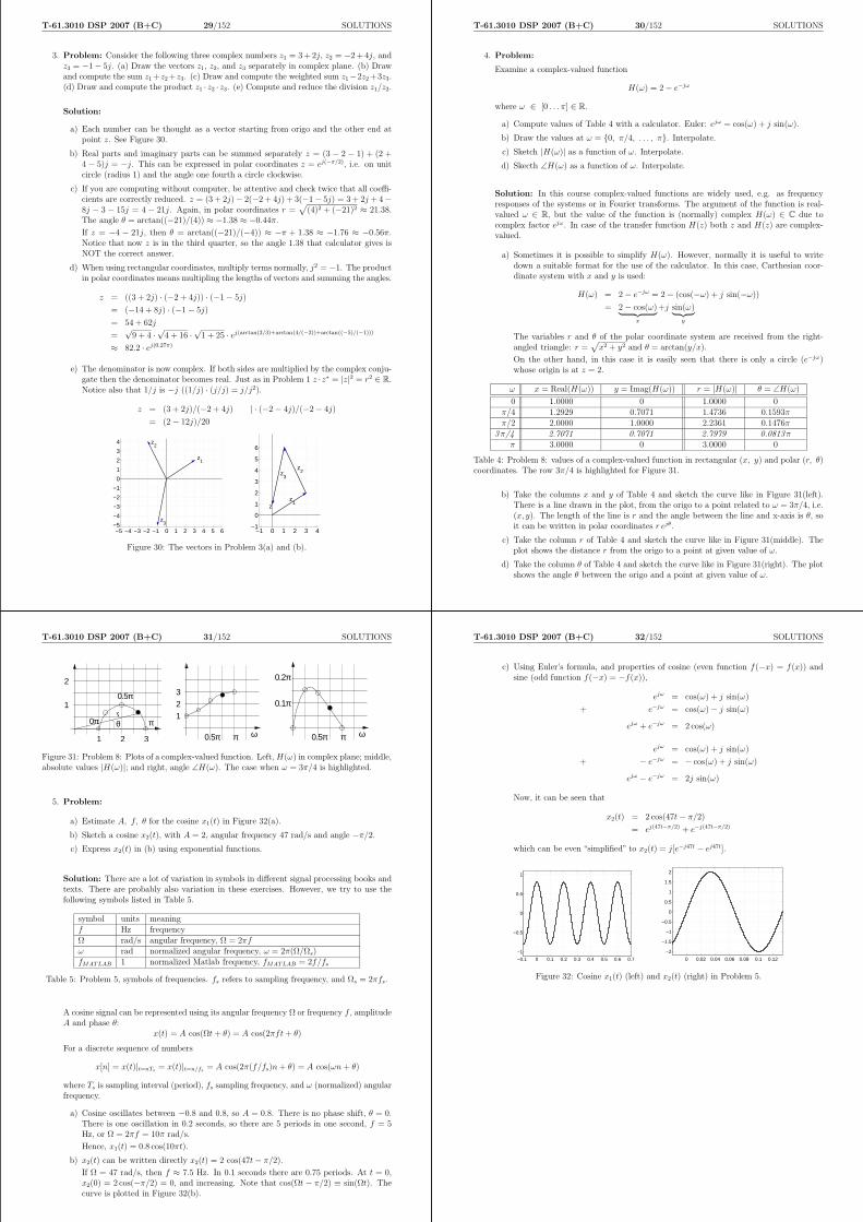
3. Problem: Consider the following three complex numbers z1 = 3 + 2j, z2 = −2 +4j, andz3 = −1− 5j. (a) Draw the vectors z1, z2, and z3 separately in complex plane. (b) Drawand compute the sum z1 +z2 +z3. (c) Draw and compute the weighted sum z1−2z2 +3z3.(d) Draw and compute the product z1 · z2 · z3. (e) Compute and reduce the division z1/z2.
Solution:
a) Each number can be thought as a vector starting from origo and the other end atpoint z. See Figure 30.
b) Real parts and imaginary parts can be summed separately z = (3 − 2 − 1) + (2 +4 − 5)j = −j. This can be expressed in polar coordinates z = ej(−π/2), i.e. on unitcircle (radius 1) and the angle one fourth a circle clockwise.
c) If you are computing without computer, be attentive and check twice that all coeffi-cients are correctly reduced. z = (3 + 2j)− 2(−2 + 4j) + 3(−1− 5j) = 3 + 2j + 4−8j − 3 − 15j = 4 − 21j. Again, in polar coordinates r =
√
(4)2 + (−21)2 ≈ 21.38.The angle θ = arctan((−21)/(4)) ≈ −1.38 ≈ −0.44π.
If z = −4 − 21j, then θ = arctan((−21)/(−4)) ≈ −π + 1.38 ≈ −1.76 ≈ −0.56π.Notice that now z is in the third quarter, so the angle 1.38 that calculator gives isNOT the correct answer.
d) When using rectangular coordinates, multiply terms normally, j2 = −1. The productin polar coordinates means multipling the lengths of vectors and summing the angles.
z = ((3 + 2j) · (−2 + 4j)) · (−1− 5j)
= (−14 + 8j) · (−1− 5j)
= 54 + 62j
=√
9 + 4 ·√
4 + 16 ·√
1 + 25 · ej(arctan(2/3)+arctan(4/(−2))+arctan((−5)/(−1)))
≈ 82.2 · ej(0.27π)
e) The denominator is now complex. If both sides are multiplied by the complex conju-gate then the denominator becomes real. Just as in Problem 1 z ·z∗ = |z|2 = r2 ∈ R.Notice also that 1/j is −j ((1/j) · (j/j) = j/j2).
z = (3 + 2j)/(−2 + 4j) | · (−2− 4j)/(−2− 4j)
= (2− 12j)/20
−5 −4 −3 −2 −1 0 1 2 3 4 5 6−5
−4
−3
−2
−1
0
1
2
3
4
z1
z2
z3
−1 0 1 2 3 4−1
0
1
2
3
4
5
6
zz
1
z2z
3
Figure 30: The vectors in Problem 3(a) and (b).
T-61.3010 DSP 2007 (B+C) 30/152 SOLUTIONS
4. Problem:
Examine a complex-valued function
H(ω) = 2− e−jω
where ω ∈ [0 . . . π] ∈ R.
a) Compute values of Table 4 with a calculator. Euler: ejω = cos(ω) + j sin(ω).
b) Draw the values at ω = 0, π/4, . . . , π. Interpolate.
c) Sketch |H(ω)| as a function of ω. Interpolate.
d) Skecth ∠H(ω) as a function of ω. Interpolate.
Solution: In this course complex-valued functions are widely used, e.g. as frequencyresponses of the systems or in Fourier transforms. The argument of the function is real-valued ω ∈ R, but the value of the function is (normally) complex H(ω) ∈ C due tocomplex factor ejω. In case of the transfer function H(z) both z and H(z) are complex-valued.
a) Sometimes it is possible to simplify H(ω). However, normally it is useful to writedown a suitable format for the use of the calculator. In this case, Carthesian coor-dinate system with x and y is used:
H(ω) = 2− e−jω = 2− (cos(−ω) + j sin(−ω))
= 2− cos(ω)︸ ︷︷ ︸
x
+j sin(ω)︸ ︷︷ ︸
y
The variables r and θ of the polar coordinate system are received from the right-angled triangle: r =
√
x2 + y2 and θ = arctan(y/x).
On the other hand, in this case it is easily seen that there is only a circle (e−jω)whose origin is at z = 2.
ω x = Real(H(ω)) y = Imag(H(ω)) r = |H(ω)| θ = ∠H(ω)
0 1.0000 0 1.0000 0π/4 1.2929 0.7071 1.4736 0.1593ππ/2 2.0000 1.0000 2.2361 0.1476π
3π/4 2.7071 0.7071 2.7979 0.0813ππ 3.0000 0 3.0000 0
Table 4: Problem 8: values of a complex-valued function in rectangular (x, y) and polar (r, θ)coordinates. The row 3π/4 is highlighted for Figure 31.
b) Take the columns x and y of Table 4 and sketch the curve like in Figure 31(left).There is a line drawn in the plot, from the origo to a point related to ω = 3π/4, i.e.(x, y). The length of the line is r and the angle between the line and x-axis is θ, soit can be written in polar coordinates r ejθ.
c) Take the column r of Table 4 and sketch the curve like in Figure 31(middle). Theplot shows the distance r from the origo to a point at given value of ω.
d) Take the column θ of Table 4 and sketch the curve like in Figure 31(right). The plotshows the angle θ between the origo and a point at given value of ω.
T-61.3010 DSP 2007 (B+C) 31/152 SOLUTIONS
1 2
1
2
3
0π
0.5π
πrθ
0.5π π
123
ω 0.5π π
0.1π
0.2π
ω
Figure 31: Problem 8: Plots of a complex-valued function. Left, H(ω) in complex plane; middle,absolute values |H(ω)|; and right, angle ∠H(ω). The case when ω = 3π/4 is highlighted.
5. Problem:
a) Estimate A, f, θ for the cosine x1(t) in Figure 32(a).
b) Sketch a cosine x2(t), with A = 2, angular frequency 47 rad/s and angle −π/2.
c) Express x2(t) in (b) using exponential functions.
Solution: There are a lot of variation in symbols in different signal processing books andtexts. There are probably also variation in these exercises. However, we try to use thefollowing symbols listed in Table 5.
symbol units meaningf Hz frequencyΩ rad/s angular frequency, Ω = 2πfω rad normalized angular frequency, ω = 2π(Ω/Ωs)fMATLAB 1 normalized Matlab frequency, fMATLAB = 2f/fs
Table 5: Problem 5, symbols of frequencies. fs refers to sampling frequency, and Ωs = 2πfs.
A cosine signal can be represented using its angular frequency Ω or frequency f , amplitudeA and phase θ:
x(t) = A cos(Ωt + θ) = A cos(2πft + θ)
For a discrete sequence of numbers
x[n] = x(t)|t=nTs = x(t)|t=n/fs = A cos(2π(f/fs)n + θ) = A cos(ωn + θ)
where Ts is sampling interval (period), fs sampling frequency, and ω (normalized) angularfrequency.
a) Cosine oscillates between −0.8 and 0.8, so A = 0.8. There is no phase shift, θ = 0.There is one oscillation in 0.2 seconds, so there are 5 periods in one second, f = 5Hz, or Ω = 2πf = 10π rad/s.
Hence, x1(t) = 0.8 cos(10πt).
b) x2(t) can be written directly x2(t) = 2 cos(47t− π/2).
If Ω = 47 rad/s, then f ≈ 7.5 Hz. In 0.1 seconds there are 0.75 periods. At t = 0,x2(0) = 2 cos(−π/2) = 0, and increasing. Note that cos(Ωt − π/2) ≡ sin(Ωt). Thecurve is plotted in Figure 32(b).
T-61.3010 DSP 2007 (B+C) 32/152 SOLUTIONS
c) Using Euler’s formula, and properties of cosine (even function f(−x) = f(x)) andsine (odd function f(−x) = −f(x)),
ejω = cos(ω) + j sin(ω)
+ e−jω = cos(ω)− j sin(ω)
ejω + e−jω = 2 cos(ω)
ejω = cos(ω) + j sin(ω)
+ − e−jω = − cos(ω) + j sin(ω)
ejω − e−jω = 2j sin(ω)
Now, it can be seen that
x2(t) = 2 cos(47t− π/2)
= ej(47t−π/2) + e−j(47t−π/2)
which can be even “simplified” to x2(t) = j[e−j47t − ej47t].
−0.1 0 0.1 0.2 0.3 0.4 0.5 0.6 0.7
−1
−0.5
0
0.5
1
0 0.02 0.04 0.06 0.08 0.1 0.12
−2
−1.5
−1
−0.5
0
0.5
1
1.5
2
Figure 32: Cosine x1(t) (left) and x2(t) (right) in Problem 5.

T-61.3010 DSP 2007 (B+C) 33/152 SOLUTIONS
6. Problem:
a) Compute with a calculator: log8 7.
b) The power of signal is attenuated from 10 to 0.01. How much is the attenuation indecibels?
c) Sketch the curve p(x) =∑+N
k=−N kx for various N .
d) Consider h(n) = sin(0.75πn)/(πn). What is h(0)?
e) Modulo-N operation for number x is written here as < x >N . What is < −4 >3?
f) What is the binary number (1001011)2 as a decimal number?
Solution:
a) log8 7 = loge 7/ loge 8 ≈ 1.9459/2.0794 ≈ 0.936.
Sometimes it is useful to convert, e.g., 22007 to decimal base: 22007 = 10x, taking log10
on both sides: x = 2007 log10 2 ≈ 604.1672. Now 100.1672 ≈ 1.4696, which finallygives 22007 ≈ 1.5 · 10604.
b) Decibel scales are widely used to compare two quantities. The decibel differencebetween two power levels, ∆L, is defined in terms of their power ratio W2/W1 (p.99, Rossing et al., The Science of Sound, 3rd Edition, Addison Wesley)
∆L = L2 − L1 = 10 log10 W2/W1
Now the power (square) of signal is attenuated from 10 to 0.01, so the signal isattenuated by 30 dB:
10 log10(0.01/10) = 10 log10 10−3 = −30
In case of computing amplitude response |H(ejω)|, e.g. in Matlab directly from theequation or with the command freqz, the values are squared for decibels
10 log10 |(H/H0)|2 = 20 log10 |(H/H0)|
c) If Σ confuses, open the expression! There is hardly anything to draw!
p(x) =+N∑
k=−N
kx = (−N)x + . . . + (−2)x + (−1)x + 0x + x + 2x + . . . + Nx
≡ 0, ∀N, x
d) Sinc-function is very useful in the signal processing, and it is defined sinc(x) =sin(πx)/(πx). Also it is known that sin(x)/x → 1, when x → 0, and with sinc-function sinc(0) = 1. Fourier-transform of a rectangular (box) signal produces spec-trum with shape of sinc-function, and vice versa, a signal like sinc-function has aspectrum of rectangular (box) shape.
Note that the result of the problem is not 1 nor 0,
h(n) = sin(0.75πn)/(πn) = 0.75 sin(0.75πn)/(0.75πn) = 0.75 sinc(0.75n)
h(0) → 0.75
T-61.3010 DSP 2007 (B+C) 34/152 SOLUTIONS
e) See also “circular shift of a sequence” (Mitra 2Ed Sec. 3.4.1, p. 140 / 3Ed Sec.5.4.1, p. 244 ). In the operation m modulo N , or, < m >N= r = m + kN , we findan integer k so that r is in the range 0 . . . N − 1. Now for < −4 >3 we find k = 2
< −4 >3=< −1 >3=< 2 >3= 2 = −4 + 2 · 3
Hence, < −4 >3= 2.
A circular buffer is implemented in the instruction sets of many DSPs. Assume thatthere is a buffer of size 1024 bytes, with addresses 0x0000 to 0x03FF in hexadecimals.New 8-bit (byte) samples are read into a buffer where an address counter (pointer)is increased by one each time. When the counter has the value 0x03FF , the nextvalue is < 0x0400 >0x0400= 0x0000. In other words, the oldest sample is replaced bythe newest. See Figure 33 for figures of linear and circular buffers.
0x0001
0x0002
0x03FD
0x03FE
0x03FF
0x0000
0x0000
0x03FD0x03FE
0x03FF0x0001
0x0002
Figure 33: Problem 6: linear and circular buffer.
f) The result depends on which number representation is chosen. In case of multi-bytedata types numbers can be saved in big-endian or little-endian manner. DSPs aredivided to fixed-point and floating-point processors (IEEE 754, sign bit, exponentand mantissa fields). Least significant bit (LSB) is normally the last bit, mostsignificant bit (MSB) leftmost. Negative numbers and fractions has to be considered,too. (Mitra 2Ed Sec. 8.4 / 3Ed Sec. 11.8 ) deals with all aspects of the numberrepresentation.
When both negative and positive b-bit fraction values are needed, 1001011 is con-sidered to have a sign bit first, and then fraction bits, like s∆a−1a−2 . . . a−b. Table 6contains some possible results with values b = 6 and s = 1, see also (Mitra 2Ed Table8.1, p. 557 / 3Ed Table 11.1, p. 638 ).
non-negative fixed-point 1001011 1 · 64 + 1 · 8 + 1 · 2 + 1 · 1 = 75
sign-magnitude 1∆001011 (−2s + 1)∑b
i=1 a−i2−i = −11/64 ≈ −0.1719
ones’ complement 1∆001011 −s · (1− 2−b) +∑b
i=1 a−i2−i = −52/64 ≈ −0.8125
two’s complement 1∆001011 −s +∑b
i=1 a−i2−i = −53/64 ≈ −0.8281
offset binary 1∆001011 +11/64 ≈ +0.1719
Table 6: Problem 6: Examples on binary number representations with values b = 6 and s = 1.
T-61.3010 DSP 2007 (B+C) 35/152 SOLUTIONS
7. Problem:
a) Compute roots of H(z) = z2 + 2z + 2.
b) Compute roots of H(z) = 1 + 16z−4.
c) Compute long division (4z4 − 8z3 + 3z2 − 4z + 6)/(2z − 3).
Solution: In this course roots of transfer function H(z) provide information on thebehaviour of the filter. The order of the rational polynomial H(z) = B(z)/A(z) is themaximum of the orders of B(z) and A(z).
a) The order of H(z) is 2. Using the equation for solving the second-order polynomialsz = (−b±
√b2 − 4ac)/(2a), the roots are z1 = −1 + j and z2 = −1− j. This can be
assured by multiplication (z − z1)(z − z2) = z2 − (z1 + z2)z + z1z2 = z2 + 2z + 2.
b) The order of H(z) is 4. Now, when setting H(z) = 1 + 16z−4 = 0, the equation canbe multiplied by z4 on both sides. Hence, z4 + 16 = 0 and z = 4
√−16. Because
−16 = 24 · ej(π+2πk), we get four roots using N√
z = | N√
r| · ej(2π k/N+θ/N).
Roots: zk = 2 ej(2πk/4+π/4), with k = 0 . . . 3. Again, z41 = (2ejπ/4)4 = 24ej4π/4 =
16ejπ = −16, and similarly other zk result to −16. In Figure 34 all four roots areplotted with circles.
−2 0 2−2
−1
0
1
2 z1 = 1.41 + 1.41j
r1 = 2, θ
1 = π/4
Figure 34: Problem 7(b): four roots of H(z) = 1 + 16z−4.
c) Division operation can be applied to polynomials just as for normal numbers. Polyno-mial product and division have a very close connection to the convolution operation.For example, in Matlab there is the same function conv for the both operations.
2z3 − z2 − 2
2z − 3)
4z4 − 8z3 + 3z2 − 4z + 6− 4z4 + 6z3
− 2z3 + 3z2
2z3 − 3z2
− 4z + 64z − 6
0
T-61.3010 DSP 2007 (B+C) 36/152 SOLUTIONS
8. Problem: Examine a complex-valued function (z ∈ C)
H(z) =1 + 0.5z−1 + 0.06z−2
1− 1.4z−1 + 0.48z−2
(a) Multiply both sides by z2. (b) Solve z2+0.5z+0.06 = 0. (c) Solve z2−1.4z+0.48 = 0.(d) H(z) can be written: H(z) = K · ((z − z1) · (z − z2)) / ((z − p1) · (z − p2)). What arethe five values? (e) What are the coefficients of H(z). What are the roots of H(z)? Whatis the order of the numerator polynomial of H(z)? What is the order of the denominatorpolynomial of H(z)?
Solution: In this course complex-valued functions are widely used. In case of the transferfunction H(z) both z and H(z) are complex-valued. A typical form of a transfer functionof a FIR filter is
H(z) = b0 + b1z−1 + b2z
−2 + . . . + bMz−M
and that of an IIR filter is
H(z) =b0 + b1z
−1 + b2z−2 + . . . + bMz−M
1 + a1z−1 + a2z−2 + . . . + aNz−N
a) Multiplication H(z) · (z2/z2) does not change the values of H(z), but it is moreconvenient to work with positive exponentials:
H(z) =z2 + 0.5z + 0.06
z2 − 1.4z + 0.48
b) Using the formula for second order polynomials az2 + bz + c = 0
z =−b±
√b2 − 4ac
2a
we get easily the roots z1 = −0.3, z2 = −0.2. In Matlab you can write P = [1 0.5
0.06]; roots(P).
c) Similarly, the roots p1 = 0.8, p2 = 0.6.
d) Using the notation from (b) and (c),
H(z) = K · (z + 0.3) · (z + 0.2)
(z − 0.8) · (z − 0.6)
= K · z2 + 0.5z + 0.06
z2 − 1.4z + 0.48
we can scale H(z) correctly by choosing K = 1.
e) In this case the coefficients were 1, 0.5, 0.06 in numerator polynomial (upper part),and 1, −1.4, 0.48 in denominator polynomial (bottom part).
Roots were computed in (b) and (c). In DSP we call the roots of numerator poly-nomial as “zeros”. The roots of denominator polynomial (bottom part) are “poles”.
As seen in (d) the same function H(z) can be expressed either using coefficientsor roots (and scaling factor). In the filter analysis the positions of roots give someinformation on the nature of the filter. More about this in Problem 46.

T-61.3010 DSP 2007 (B+C) 37/152 SOLUTIONS
9. Problem:
a) Decompose f(x) = 1/(x2 + 1)
b) Decompose H(z) = (0.4− 0.2z−1)/(1− 0.1z−1 − 0.06z−2)
Solution: In this course partial fractions are used when finding an explicit form of theimpulse response h[n] from the transfer function H(z). In the list of Fourier-transformpairs there are only inverse transforms for the first order expressions. So, if the trans-fer function is of second-order or higher, it has to be converted to a sum of first-orderexpressions by partial fraction decomposition (expansion).
Decomposition requires taking roots of a polynomial, so it is possible to derive by handsonly in some cases, e.g., 1/(x2 + 3x + 2) = 1/(x + 1)− 1/(x + 2). For more complicatedcases, see (Mitra 2Ed Sec. 3.9 / 3Ed Sec. 6.4 ), or any other math reference. When usingMatlab, the command is residuez.
Rules of thumb, (1) compute roots of the denominator polynomial, (2) write down the sumof first-order rational polynomials, (3) compute the unknown constants (equation pairs).Note that the decomposition in not unique, but there are several different expressionswhich lead to the same result.
a) Find the roots of the denominator: x2 + 1 = 0 ⇒ x1 = −j, x2 = j. Roots can becomplex, too! Hence,
f(x) =A
x− x1
+B
x− x2
=A
x + j+
B
x− j
=A(x− j) + B(x + j)
x2 + jx− jx + 1=
x(A + B) + j(−A + B)
x2 + 1
⇒
A + B = 0
−A + B = −j⇒
A = 0.5j
B = −0.5j
Finally,
f(x) =0.5j
x + j− 0.5j
x− j
b) In this course z−1 corresponds a unit delay in time-domain. The numerator poly-nomial can divided and z−1 terms can be taken to front, and the partial fraction isdone only once for P (z), whose numerator polynomial is plain 1,
H(z) =0.4− 0.2z−1
1− 0.1z−1 − 0.06z−2
= 0.4 · 1
1− 0.1z−1 − 0.06z−2︸ ︷︷ ︸
P (z)
−0.2z−1 · 1
1− 0.1z−1 − 0.06z−2︸ ︷︷ ︸
P (z)
The denominator of P (z) is set to zero and multiplied by z2: z2 − 0.1z − 0.06 = 0.The roots are z1 = 0.3 and z2 = −0.2.
P (z) =A
1− 0.3z−1+
B
1 + 0.2z−1=
A + 0.2Az−1 + B − 0.3Bz−1
1− 0.1z−1 − 0.06z−2
Now we get a pair of equations
A + B = 1
0.2A− 0.3B = 0⇒
A = 0.6
B = 0.4and finally,
H(z) = 0.4 ·( 0.6
1− 0.3z−1+
0.4
1 + 0.2z−1
)
− 0.2z−1 ·( 0.6
1− 0.3z−1+
0.4
1 + 0.2z−1
)
T-61.3010 DSP 2007 (B+C) 38/152 SOLUTIONS
10. Problem:
a) What is sum of series S =∑∞
k=0(0.5)k.
b) S =∑∞
k=10(−0.6)k−2.
c) S =∑∞
k=2(0.8k−2 · e−jωk).
Solution: Sum of geometric series is applied in Fourier- and z-transforms. When theratio q in geometric series is |q| < 1, the sum of series converges to
∑∞k=0 qk = 1/(1− q),
and correspondingly∑N
k=0 qk = (1− qN+1)/(1− q).
a) Directly from the formula with q = 0.5, S = 1/(1− 0.5) = 2.
b) Open Σ expression if it seems to be difficult.
S =
∞∑
k=10
(−0.6)k−2 = (−0.6)8 + (−0.6)9 + (−0.6)10 + . . .
=
∞∑
k=8
(−0.6)k
=
∞∑
k=0
(−0.6)k −7∑
k=0
(−0.6)k
= 1/(1 + 0.6)− (1− (−0.6)8)/(1 + 0.6) = (−0.6)8/1.6 ≈ 0.0105
c) Discrete-time Fourier-transform is defined as
X(ejω) =
∞∑
n=−∞
x[n]e−jωn
S =∞∑
k=2
(0.8k−2 · e−jωk) |k = m + 2
=
∞∑
m=0
(0.8m · e−jωm · e−j2ω)
= e−j2ω ·∞∑
m=0
(0.8e−jω)m
= e−j2ω · 1
1− 0.8e−jω
The term e−j2ω can be seen as a time shift (delay) of two units.
T-61.3010 DSP 2007 (B+C) 39/152 SOLUTIONS
11. Problem:
a) List all integral transforms that are used in previous signal processing courses.
b) Compute the integral X(Ω) =∫ 4
0e−jΩtdt.
Solution: A general integral transform is defined by
F (ω) =
∫ b
a
f(t)K(ω, t)dt
where K(ω, t) is an integral kernel of the transform, see e.g. (Mitra 2Ed Sec. - / 3EdSec. 5.1 ).
a) In our case the time-domain signal is transformed to the frequency-domain in orderto improve the analyse. For example, the structure of a periodic signal can be seeneasily in the spectrum.
Periodic signals can be represented as Fourier-series. Laplace- and z-transformsare more general than Fourier-transforms. There are versions for both analog anddigital signals as well as for one-dimensional and two-dimensional signals. Certaintransforms are used in particular applications, say, discrete cosine transform is usedin JPEG and wavelet transform in JPEG2000.
b) Now x(t) can be considered as a rectangular signal, and its Fourier transform is asinc-function.
X(Ω) =
∫ 4
0
e−jΩtdt =
4/
0
(1/(−jΩ))e−jΩt = (1/(−jΩ))(e−j4Ω − 1)
= (1/(−jΩ))(−e−j2Ω)(ej2Ω − e−j2Ω) = (1/(−jΩ))(−e−j2Ω)(2j sin(2Ω))
= 4e−j2Ω(sin(2Ω)/(2Ω)) = 4e−j2Ω sinc(2Ω/π)
T-61.3010 DSP 2007 (B+C) 40/152 SOLUTIONS
12. Problem: Using notation WN = e−j2π/N and matrix
D4 =
1 1 1 11 W 1
4 W 24 W 3
4
1 W 24 W 4
4 W 64
1 W 34 W 6
4 W 94
compute X = D4x, when x =[2 3 5 −1
]T
Solution: We see that
|WN | = |e−j2π/N | = | cos(2π/N)− j sin(2π/N)| =√
cos(2π/N)2 + sin(2π/N)2 = 1
That is, the points W kN are lying clockwise on the unit circle. When N = 4, the angle
between each point is π/2:
W 04 = 1 W 1
4 = −j W 24 = −1 W 3
4 = jW 4
4 = 1 W 54 = −j W 6
4 = −1 W 37 = j
W 84 = 1 W 9
4 = −j
The square matrix D4 is
D4 =
1 1 1 11 −j −1 j1 −1 1 −11 j −1 −j
Size of matrix D4 is 4 rows and 4 columns (4× 4), and that of column vector x is (4× 1).In the matrix product X = D4x dimensions must agree: (4× 4)(4× 1), and the final sizeof X is (4× 1).
X = D4x =
1 1 1 11 −j −1 j1 −1 1 −11 j −1 −j
235−1
=
1 · 2 + 1 · 3 + 1 · 5 + 1 · (−1)1 · 2− j · 3− 1 · 5 + j · (−1)1 · 2− 1 · 3 + 1 · 5− 1 · (−1)1 · 2 + j · 3− 1 · 5− j · (−1)
=
9−3− 4j
5−3 + 4j
We have computed here discrete Fourier transform (DFT) for a real sequence 2, 3, 5, −1.The result, here 9, −3−4j, 5, −3+4j, is often complex-valued. There are several sym-metric properties of DFT that are discussed later.
The matrix D∗4 (Hermitian) is transpose of D4 with complex-conjugate values:
D∗4 =
1 1 1 11 j −1 −j1 −1 1 −11 −j −1 j

T-61.3010 DSP 2007 (B+C) 41/152 SOLUTIONS
13. Problem: Consider an analog signal x(t) = π · cos(2πt). Plot the analog signal, thediscrete-time signal sampled with 5 Hz, and the digital signal with accuracy to integernumbers.
Solution: Analog signal: both t and x(t) ∈ R. You can measure the outside tempera-ture at any time exactly.
Discrete-time signal: signal x[n] may get any values at certain time moments, x[n] ∈R, n ∈ Z. Often explained as a sampled version of analog signal.
Digital signal: signal x[n] is discrete also with amplitude values, n, x[n] ∈ Z.
Here x(t) = π · cos(2πt). The angular frequency is Ω = 2π rad/s and the frequency f = 1Hz while Ω = 2πf . The period of the signal is T = 1/f = 1 second.
The sampling frequency is fs = 5 Hz, i.e., samples are taken every Ts = 0.2 seconds:t← nTs. This gives a discrete-time sequence
x[n] = π · cos(0.4πn)
where the normalized angular frequency is ω = 0.4π rad/sample.
The numeric values are below in a table. The plots in Figure 35, where in (a) t runs from0 to 2.5 seconds, and in (b) and (c) n correspondingly from 0 to 12.
t n (a) x(t) (b) x[n] (c) x[n]0 0 π · cos(0) = π π Intπ = 30 < t < 0.2 ∄ cos(2πt) ∄ ∄0.2 1 π · cos(0.4π) ≈ 0.9708 ≈ 0.9708 Int0.9708 = 11 5 π · cos(2π) = π π Intπ = 3
0 0.5 1 1.5 2 2.5−4
−3
−2
−1
0
1
2
3
4
x(1)=π
0 2 4 6 8 10 12−4
−3
−2
−1
0
1
2
3
4x[0]=π
x[1]=cos(0.4π)
x[2]
x[5]=π
0 2 4 6 8 10 12−4
−3
−2
−1
0
1
2
3
4x[0]=3
x[1]=1
x[3]=−3
x[5]=3
Figure 35: Problem 13: (a) analog signal, (b) discrete-time signal, (c) digital signal.
Definitions may vary from book to book. Discrete-time or digital signal is often called asequence instead of signal.
In practice, A/D converted discretizes the analog signal into digital signal with a certainaccuracy. For instance, in audio recordings (CD quality) the sampling frequency is 44100Hz (44100 samples each second) and the each data sample is expressed with 16 bits, i.e.,having 216 = 65536 discrete levels.
Note also that π is an irrational number which cannot be expressed accurately with finitenumber of bits.
T-61.3010 DSP 2007 (B+C) 42/152 SOLUTIONS
14. Problem: The unit impulse function δ[n] and the unit step function µ[n] (or u[n]) aredefined
δ[n] =
1, when n = 0
0, when n 6= 0µ[n] =
1, when n ≥ 0
0, when n < 0
Sketch the following sequences around the origo (a) x1[n] = sin(0.1πn), (b) x2[n] =sin(2πn), (c) x3[n] = δ[n − 1] + δ[n] + 2δ[n + 1], (d) x4[n] = δ[−1] + δ[0] + 2δ[1], (e)x5[n] = µ[n]− µ[n− 4], (f) x6[n] = x3[−n + 1].
Solution: There are different ways to draw discrete-time signals. Here we use “pins”or “stems”, which emphasizes that the sequence is discrete-time. Compute the values foreach n using sin(), δ[n], µ[n] functions, for example, in (c)
n δ[n− 1] δ[n] 2δ[n + 1] x[n]-2 δ[−2− 1] = 0 δ[−2] = 0 2δ[−2 + 1] = 0 0 + 0 + 0 = 0-1 δ[−1− 1] = 0 δ[−1] = 0 2δ[−1 + 1] = 2 0 + 0 + 2 = 20 δ[0− 1] = 0 δ[0] = 1 2δ[0 + 1] = 0 0 + 1 + 0 = 11 δ[1− 1] = 1 δ[1] = 0 2δ[1 + 1] = 0 1 + 0 + 0 = 12 δ[2− 1] = 0 δ[2] = 0 2δ[2 + 1] = 0 0 + 0 + 0 = 0
See the results in Figure 36. Note that in (b) the argument for the sine function is always2π-multiple. In (d) there are only constants δ[−1] = δ[1] = 0 and δ[0] = 1 from thedefinition.
The discrete-time signal is purely a sequence of numbers, e.g. in (c), x3[n] = 2, 1, 1,where the underlined position is at n = 0. Non-zero values can be also listed, e.g.,x3[−1] = 2, x3[0] = 1, and x3[1] = 1.
−10 0 10−1
0
1
(a)
−5 0 5−1
0
1
(b)
−2 −1 0 1 2
0
1
2
(c)
−5−4−3−2−1012345
0
0.5
1
(d)
−3−2−1 0 1 2 3 4 5
0
0.5
1
(e)
−2 −1 0 1 2
0
1
2
(f)
Figure 36: Sequences of Problem 14. Top row: (a)-(c), bottom: (d)-(f).
T-61.3010 DSP 2007 (B+C) 43/152 SOLUTIONS
15. Problem: Which of the following signals are periodic? Define the length of the fundamen-tal period and frequency for periodic signals. (a) x(t) = 3 cos(8π
31t), (b) x[n] = 3 cos(8π
31n),
(c) x(t) = cos(π8t2), (d) x[n] = 2 cos(π
6n−π/8)+sin(π
8n), (e) x[n] = . . . , 2, 0, 1, 2, 0, 1, 2, 0, 1, . . .,
(f) x[n] =∑+∞
k=−∞ δ[n− 4k] + δ[n− 4k − 1].
Solution: Continuous-time signal x(t) is periodic, if there exists period T ∈ R, forwhich x(t) = x(t + T ), ∀t. The fundamental period is the smallest T0 > 0.
Discrete-time signal (sequence) x[n] is periodic, if there exists period N ∈ Z, for whichx[n] = x[n + N ], ∀n ∈ Z. The fundamental period is the smallest N0 > 0.
The analysis is often done for sines or cosines which are 2π-periodic. Replace t by t + T(n by n + N) and try if the equation x(t) = x(t + T ) holds. Note that the amplitudeor phase shift does not have effect on periodicity. The exponential function ejω is also2π-periodic.
Another way to find the period of sine is to express the function in form of x(t) =sin(2π · f · t) where f is frequency (Ω = 2πf is angular frequency). Then T = 1/f .
If there is a sum of cosines, like in (d), one has to find period T0 (N0), to which all periodsof individual cosines are multiples. Correspondingly, in frequency domain one has to finda fundamental frequency f0, with which all individual frequencies can be represented.
a) Periodic. When T = (31/4)k, then the original cosine argument is added 2π-multiple,and x(t) = x(t+T ) holds. The fundamental period is the shortest period T0 = 31/4.
x(t) = 3 cos(8π
31t) = 3 cos(
8π
31(t + T )) = 3 cos(
8π
31t +
8π
31T )
= 3 cos(8π
31t + 2π(
4
31T ))
b) Periodic, N0 = (31/4) · k. The period N0 has to be integer, so the smallest possiblek = 4 gives the length of the fundamental period N0 = 31.
x[n] = 3 cos(8π
31n) = 3 cos(
8π
31(n + N)) = 3 cos(
8π
31n +
8π
31N)
= 3 cos(8π
31n + 2π(
4
31N))
Notice also the difference of the results in (a) and (b), where x(t) = x(t + (31/4)),but x[n] = x[n + 31]. The signals are plotted in the same axis in Figure 37.
0 5 10 15 20 25 30 35−3
−2
−1
0
1
2
3
(a) vs (b): x(t) = 3cos(8π / 31 t) vs x[n] = 3cos(8π / 31 n)
n, t
T=31/4N=31
x(t)x[n]
Figure 37: A visualization of the difference of fundamental periods of similar looking analogand discrete-time signals in Problem 15(a) and (b). T0 = 31/4 but N0 = 31.
T-61.3010 DSP 2007 (B+C) 44/152 SOLUTIONS
c) Non-periodic, the latter term depends on t. The result can be also seen in Fig-ure 38(c).
x(t) = cos(π
8t2) = cos(
π
8(t + T )2) = cos(
π
8t2 +
π
8(2tT + T 2))
= cos(π
8t2 + 2π(
tT
8+
T 2
16))
d) Periodic, N0 = 48. The fundamental period is the least common multiple (LCM)of individual periods N1 = 12, N2 = 16 ⇒ N0 = 4N1 = 3N2 = 48. On the otherhand the fundamental angular frequency is the greatest common divisor (GCD)of individual frequencies (ω = 2π/N): ω1 = π/6, ω2 = π/8 ⇒ ω0 = π/24,⇒ω1 = 4ω0, ω2 = 3ω0. More about computing LCM and GCD can be found, e.g.“Beta, Mathematics Handbook for Science and Engineering”. There are Matlabcommands lcm and gcd, too.
x[n] = 2 cos(π
6n− π/8) + sin(
π
8n) = 2 cos(2π
1
12n− π/8) + sin(2π
1
16n)
e) (Assume that) the period is N0 = 3, i.e. x[0] = x[±3k] = 2, x[1] = x[±3k + 1] = 0,x[2] = x[±3k + 2] = 1, where the integer k > 0.
f) N0 = 4. “Open” the sequence if you do not see it directly:
x[n] =
+∞∑
k=−∞
δ[n− 4k] + δ[n− 4k − 1]
= . . . + δ[n + 4] + δ[n + 4− 1]︸ ︷︷ ︸
k=−1
+ δ[0] + δ[n− 1]︸ ︷︷ ︸
k=0
+ δ[n− 4] + δ[n− 4 + 1]︸ ︷︷ ︸
k=1
+ . . .
= . . . , 1, 1, 0, 0, 1, 1, 0, 0, 1, 1, 0, 0, . . .
Periodicity of signal is often easy to see from the signal plot, see Figure 38. The signal (c)is clearly not periodic. Real-life signals (e.g. speech signal) are seldom periodic in strictsense; almost periodic signals are sometimes called “quasi-periodic”.
0 20 40
−2
0
2
(a)
0 20 40
−2
0
2
(b)
0 5 10
−1
−0.5
0
0.5
1
(c)
0 20 40 60 80
−2
0
2
(d)
n−5 0 5
0
1
2
(e)
n−5 0 5
0
0.5
1
1.5
(f)
n
Figure 38: Signals and sequences in Problem 15, (a)..(c) in top row, (d)..(f) in bottom row. Itcan be seen that (at least) (c) is not periodic in the scene shown.

T-61.3010 DSP 2007 (B+C) 45/152 SOLUTIONS
16. Problem: There’s a sequence 5, 3,−1, 2,−5,−7. Compute “a two-point moving aver-age”.
Solution: The avaraged sequence is (5 + 3)/2, (3− 1)/2, (−1 + 2)/2, (2− 5)/2, (−5−7)/2 = 4, 1, 0.5, −1.5, −6.The input sequence is x[n] = 5, 3, −1, 2, −5, −7, i.e., x[0] = 5, x[1] = 3, x[2] =2, x[3] = −5, x[4] = −7. The averaging process can be thought as a filtering operation:
y[n] =x[n] + x[n− 1]
2
This results to a LTI system with the impulse response
h[n] =δ[n] + δ[n− 1]
2
and the frequency response
H(ω) =1 + e−jω
2
which in DSP literature is normally written as H(ejω). The corresponding flow (block)diagram is plotted in Figure 39.
Slow changes in the signal (temperature) mean low frequencies and quick changes meanhigh frequencies. Averaging smoothens the signal. In DSP, we say that it is a lowpassfilter while it preserves low frequencies in the signal but attenuates high frequencies.High-frequency variation is often considered as noise.
D
x[n] y[n]
0.5
Figure 39: Problem 16: Flow diagram of the filter.
T-61.3010 DSP 2007 (B+C) 46/152 SOLUTIONS
17. Problem: Express the input-output relations of the discrete-time systems in Figure 41.
Solution: In this problem there are several types of discrete-time systems. Notice thatthe scope of this course is LTI systems (linear and time-invariant). LTI systems are veryeasy to detect, they are relatively simple but very useful. In this course the system inputx[n] and output y[n] are 1-dimensional except some examples with pictures (2D). ForLTI-systems the input-output relation can be written with a difference equation or a setof difference equations.
There are some basic operations on sequences (signals) in discrete-time systems (x refersto input to the system / operation, y output) shown also in Figure 40:
• sum of signals (sequences) y[n] = x1[n] + x2[n]
• signal multiplication (by constant) y[n] = a x[n]
• delay or advance of signal y[n] = x[n± k]
• product of signals, modulator (non-LTI systems) y[n] = x1[n] · x2[n]
• branch / pick-off node y1[n] = x[n], y2[n] = x[n]
x[n]
x[n]
x[n−1]D
zx[n−1]−1
x[n]a
ax[n]
x [n]+x [n]21
x [n] . x [n]21
x [n]
x [n]1
2 x [n]
x [n]1
2
x[n]
x[n]x[n]
(a) (d)(b) (c) (e)
Figure 40: Problem 17: Basic operations in discrete-time systems, (a) sum of sequencies, (b)amplification by constant, (c) unit delay (D, T , or z−1), and (d) product of signals, modulator(non-LTI systems), and (e) branch / pick-off node.
D
D
y[n]x[n]
−2x[n−1]
x[n−2]
(a)
z−1z−1
z−1
x[n]
−2 2
y[n]
x[n−1]
x[n−2]
y[n−1]
y[n]y[n]
(b)
x[n] y[n]
cos( n)ω
(c)
v[n]+
+c
x[n]
y[n]
a b
D
(d)
Figure 41: Problem 17: Discrete-time systems, also at page 9.
T-61.3010 DSP 2007 (B+C) 47/152 SOLUTIONS
a) Difference equation: y[n] = x[n] − 2x[n − 1] + x[n − 2]. LTI-filter, type FIR (seeProblem 18).
b) The memory registers / unit delays are often drawn either “D” (delay) or “z−1 (refersto a delay in z-transform). Note that the output is fed back in the loop. The leftpart of the filter is the same as (a). The sequence right after the second summing ontop line is y[n] which goes both to the output and down to feedback loop. Thereforethe terms coming into the last summing unit are x[n]− 2x[n− 1]+x[n− 2] from leftand 2y[n− 1] from the loop. The difference equation is
y[n] = 2y[n− 1] + x[n]− 2x[n− 1] + x[n− 2]
The system is LTI and type IIR (see Problem 18).
c) Input signal x[n] is multiplied by a sequence cos(ωn) (not a constant). This operationis called modulation and is not LTI. The relation can be written as
y[n] = x[n] · cos(ωn)
d) This is so called lattice structure (Mitra 2Ed Sec. 6 / 3Ed Sec. 8 ). In order to getrelationship between x[n] and y[n] temporary variables are used after each summingunit. In this case, there is one temporary variable v[n], and the set of differenceequations is
v[n] = x[n] + a v[n− 1]
y[n] = b v[n] + c v[n− 1]
The temporary variable v[n] can be simplified away, but it is easier to determinethe transfer function H(z) in frequency domain and then apply inverse z-transform,which is discussed later. The system is LTI and IIR (see Problem 18).
Remark. The simplified difference equation for the system in (d) can be received byeliminating all temporary v[n] sequences:
x[n] = v[n]− a v[n− 1] | x on left side
y[n] = b v[n] + c v[n− 1] | y on left side
−bx[n] = −b v[n] + ab v[n− 1] | y[n]− bx[n] cancels v[n]
−ay[n− 1] = −ab v[n− 1]− ac v[n− 2]
−cx[n − 1] = −c v[n− 1] + ac v[n− 2] | all v[n− 1], v[n− 2] cancelled
which finally gives y[n] = ay[n− 1] + bx[n] + cx[n− 1].
The discrete-time system does some computation for sequencies of numbers. Therefore itis straightforward to write down a computer program, e.g. in (a),
x1 := 0; x2 := 0;
while TRUE
x2 := x1;
x1 := x0;
x0 := read_next_input(input_stream);
y := x0 - 2*x1 + x2;
write_output(output_stream, y);
or if all samples are known and in a vector,
for (k = 2; k <= length(x); k++)
y[k] := x[k] - 2*x[k-1] + x[k-2];
T-61.3010 DSP 2007 (B+C) 48/152 SOLUTIONS
18. Problem: Look at the flow (block) diagrams in Figure 42.
x[n] y[n]
-0.75
0.5
z-1
z-1
i
0.5 -0.75
y[n]x[n]
-1z -1z
ii
0.5
x[n]
0.5
0.75
-0.75
y[n]
z-1
z-1
iii
1
y[n]1/2x[n]
iv
v[n]+
+c
x[n]
y[n]
a b
D
v
Figure 42: Flow diagrams of Problem 18, also at page 9.
a) What does LTI mean? How to prove or recognise LTI systems?
b) Which systems are linear and time-invariant (LTI)?
c) Which systems have feedback?
d) Which LTI systems are FIR and which are IIR?
Solution: In this problem we try to recognise LTI systems by their layout.
a) LTI = linear AND time-invariant (=shift-invariant) system. These two propertiesbelong to a system not to a signal. Other system properties can be, e.g. stability,causality, or if it needs memory or if it can be inverted.
See Problem 19 for mathematical proofs.
Recognition of LTI systems from the flow (block) diagrams: there are only (1) sumsof signals, (2) multiplication by a contant, (3) delays or advances. The componentswere introduced in Problem 17, see Figure 40 at page 46.
LTI systems can be represented with a linear constant coefficient difference (or dif-ferential in case of analog system) equation
∑
k
dk y[n− k] =∑
k
pk x[n− k]
where dk and pk are constants. Often in practice, we use causal finite-dimensionalLTI systems
∑Nk=0 dk y[n− k] =
∑Mk=0 pk x[n − k], where the order of the system is
given by maxN, M (Mitra 2Ed Sec. 2.6.0 / 3Ed Sec. 2.7.0 ). If the system cannotbe written in the format above, it is not a (causal) LTI system.
b) LTI? Only summing, delays, amplifications by constants. (i) Yes, (ii) Yes, (iii) Yes,(iv) No, adding a constant, (v) Yes.
c) Feedback means that some of the output (or internal) values are fed back in thesystem. Computation can be said to be recursive or iterative. There are loops in (i),(ii), (iii), and (v).
d) FIR = Finite (length) Impulse Response. IIR = Infinite (length) Impulse Response.
If the system has a feedback loop somewhere in the structure, it is also IIR at thesame time. The output value is computed using older output values, i.e. there isrecursion. This can be seen that there are also terms y[n−k], k 6= 0, in the differenceequation.
If there is no loop and computation flows forward all the time, then the system isFIR. This can be seen that there is only the term y[n] in the left side of the differenceequation above.
FIR: (iv) has an impulse response of finite length but it is not LTI. IIR: (i), (ii), (iii),and (v) have infinite (length) impulse response because of feedback loops.

T-61.3010 DSP 2007 (B+C) 49/152 SOLUTIONS
19. Problem: Determine if the system is (1) linear, (2) causal, (3) stable, and (4) shift-invariant.
a) y[n] = x3[n],
b) y[n] = γ +∑2
l=−2 x[n− l], γ is a nonzero constant,
c) y[n] = αx[−n], α is a nonzero constant.
Solution: Properties of the discrete-time system, see (Mitra 2Ed Sec. 2.4.1, 2.5.3, 2.5.4/ 3Ed Sec. 2.4.2, 2.5.3., 2.5.4 ).
Linearity:If y1[n] and y2[n] are the responses to the input sequences x1[n] and x2[n], respectively,then for an input
x[n] = αx1[n] + βx2[n],
the response is given byy[n] = αy1[n] + βy2[n].
x 1
x 2
x
b
*3
S
a
b
y3
a1
y2
y3
yx 1
x 2
S
S
Figure 43: Linearity. If the linear combination of outputs of x1 and x2 is the same as the outputof the linear combination of inputs, then the system is linear.
Remark. When considering a constant-coefficient difference equation like y[n]+0.5y[n−1] = x[n] + 0.5x[n− 1] the system is not linear, if the initial conditions are not zero, i.e.,y[−1] 6= 0. When initial values are zero, the system is said to be in rest. See (Mitra 2EdEx. 2.30, p. 92 / 3Ed Ex. 2.37, p. 92 ).
Causality:The n0-th output sample y[n0] depends only on previous output values and input samplesx[n] for n ≤ n0, and does not depend on input samples for n > n0. In case of LTI-system,the system is causal if and only if impulse response h[n] = 0 for all n < 0.
Stability:Bounded input, bounded output (BIBO) stability: If a bounded input (Bx is a finiteconstant)
|x[n]| < Bx <∞, ∀nproduces a bounded output (By is a finite constant)
|y[n]| < By <∞, ∀n
as a response then the system is BIBO stable (see (a) and (b) at Page 50 for details). Incase of LTI-system, the system is stable if and only if
∑∞n=−∞ |h[n]| <∞.
Time/Shift-invariance:If y1[n] is the response to an input x1[n], then the response to an input
x[n] = x1[n− n0]
T-61.3010 DSP 2007 (B+C) 50/152 SOLUTIONS
1
D kS2 y 1*yx 1 [n-k]= y
2x 1xD k
x 1 [n-k]S
y 2=
Figure 44: Time invariance. If the output of delayed input is the same as delayed output, thenthe system is time-invariant.
is simplyy[n] = y1[n− n0],
where n0 is any positive or negative integer.
a) y[n] = x3[n].
Take inputs x1[n] and x2[n], the outputs are then y1[n] = x31[n] and y2[n] = x3
2[n].Now the linear combination of the input signals is x3[n] = αx1[n] + βx2[n] and theoutput is
y3[n] = (αx1[n] + βx2[n])3 6= αx31[n] + βx3
2[n] = αy1[n] + βy2[n].
Hence the system is not linear.
Since there is no output before the input hence the system is causal.
The system is stable: Assume |x[n]| < Bx, then
|y[n]| = |x3[n]| ≤ |x[n]|3 < B3x = By <∞.
The system is time-invariant: Assume input x1[n] and output y1[n], then responseof input x[n] = x1[n− n0] is
y[n] = (x[n])3 = (x1[n− n0])3 = y1[n− n0]
b) y[n] = γ +∑2
l=−2 x[n− l], γ is a nonzero constant.
Use linear combination αx1[n] + βx2[n] as the input
y3[n] = γ +2∑
l=−2
(αx1[n− l] + βx2[n− l])
= 0.5γ + α
2∑
l=−2
x1[n− l] + 0.5γ + β
2∑
l=−2
x2[n− l]
6= αγ + α
2∑
l=−2
x1[n− l] + βγ + β
2∑
l=−2
x2[n− l]
= αy1[n] + βy2[n],
where α and β are not fixed. The system is hence nonlinear.
The system is not causal, because there can be output before input, when l ∈[−2,−1].
System is stable: Assume bounded input |x[n]| < Bx, then
|y[n]| = |γ +
2∑
l=−2
x[n− l]| ≤ |γ|+2∑
l=−2
|x[n− l]| < |γ|+ 5Bx = By <∞
T-61.3010 DSP 2007 (B+C) 51/152 SOLUTIONS
The system is also time-invariant: Assume input x1[n] and output y1[n], thenresponse of input x[n] = x1[n− n0] is
y[n] = γ +
2∑
l=−2
x1[n− n0] = y1[n− n0].
c) y[n] = αx[−n], α is a nonzero constant.
The system is linear, stable and noncausal.
Assume inputs x1[n],x[n] and outputs y1[n], y[n] , respectively, then
y[n] = αx[−n],
y1[n] = αx1[−n].
Let x[n] = x1[n− n0], then
y[n] = αx[−n] = αx1[−n− n0]
6= αx1[n0 − n] = αx1[−(n− n0)] = y1[n− n0]
and the system is not time-invariant.
T-61.3010 DSP 2007 (B+C) 52/152 SOLUTIONS
20. Problem: A LTI system with an input x1[n] = 1, 1, 1 gives an output y1[n] =0, 2, 5, 5, 3. If a new input is x2[n] = 1, 3, 3, 2, what is the output y2[n]?
Solution: The system is both linear (L) and time-invariant (TI). Now x2[n] can bethought as a sum of original x1[n] and a shifted and scaled 2x1[n− 1]:
x2[n] = x1[n] + 2x1[n− 1] = 1, 1, 1+ 0, 2, 2, 2 = 1, 3, 3, 2
Because of LTI, the output y2[n] is also a sum of original y1[n] and a shifted and scaled2y1[n− 1], as shown in Figure 45
y2[n] = y1[n] + 2y1[n− 1] = 0, 2, 5, 5, 3+ 0, 0, 4, 10, 10, 6 = 0, 2, 9, 15, 13, 6
0 2 4 6
0123
n
x 1[n]
0 2 4 6
0123
n
2 x 1[n
−1]
0 2 4 6
0123
n
x 2[n]
0 2 4 60
5
10
15
n
y 1[n]
0 2 4 60
5
10
15
n
2 y 1[n
−1]
0 2 4 60
5
10
15
n
y 2[n]
Figure 45: Problem 20: Left column: sequences x1[n], 2x1[n−1], and x2[n] = x1[n]+2x1[n−1].Right column: sequences y1[n], 2y1[n− 1], and y2[n] = y1[n] + 2y1[n− 1]. This holds for linearand time-invariant (LTI) systems.
Remark: A standard way to solve this problem is to compute deconvolution of x1[n] andy1[n], and then apply the result to the new input x2[n]. See Problem 26.

T-61.3010 DSP 2007 (B+C) 53/152 SOLUTIONS
21. Problem:
a) What is the impulse response of the system in Figure 46(a)? What is the connectionto the difference equation? Is this LTI system stable/causal?
b) What are the first five values of impulse response of the system in Figure 46(b)?
c) What are the first five values of impulse response of the system in Figure 46(d)?
D
D
y[n]x[n]
−2x[n−1]
x[n−2]
(a)
z−1z−1
z−1
x[n]
−2 2
y[n]
x[n−1]
x[n−2]
y[n−1]
y[n]y[n]
(b)
v[n]+
+c
x[n]
y[n]
a b
D
(d)
Figure 46: Discrete-time systems for Problems 21 and 22.
Solution: Impulse response h[n] is the response of the system to the input δ[n]. LTIdiscrete-time system is completely specified by its impulse response h[n] (Mitra 2Ed Sec.2.5.1 / 3Ed Sec. 2.5.1 ). For a LTI system (see Problems 18 and 19) the stability conditionis∑
n |h[n]| <∞ and the causability condition h[n] = 0, ∀n < 0.
If the impulse response h[n] is known for a LTI system, then the output y[n] can becomputed for any input x[n] by convolution.
Impulse δ[n] −→ Any discrete-timesystem
−→ Impulse responsehi[n]
Input sequence x[n] −→ Discrete-timeLTI system h[n]
−→ Output sequence y[n]y[n] = h[n] ⊛ x[n]
a) Difference equation of the system is y[n] = x[n]− 2x[n− 1]+ x[n− 2]. Let the inputbe δ[n] and read what comes out.
n x[n] = δ[n] −2x[n− 1] x[n− 2] y[n] = x[n]− 2x[n− 1] + x[n− 2]. . . 0 0 0 0-1 0 0 0 00 1 0 0 11 0 -2 0 -22 0 0 1 13 0 0 0 0
. . . 0 0 0 0
The impulse response is
h[n] = δ[n]− 2δ[n− 1] + δ[n− 2]
The length L. of the impulse response is finite, Lh[n] = 3 <∞. So, the filter isFIR (finite impulse response).
T-61.3010 DSP 2007 (B+C) 54/152 SOLUTIONS
Notice that in case of FIR filter (no feedbacks, flow always going forward), theimpulse response can be easily gotten from the corresponding difference equationjust by replacing y by h and each x by δ (Mitra 2Ed Sec. 2.5.1 / 3Ed Sec. 2.5.1 ).
All FIR systems are always stable because the length of impulse response is finite,and therefore also the sum of absolute values is finite:
∑|h[n]| < ∞, in this case
∑|h[n]| = 1 + 2 + 1 = 4 <∞.
This FIR system is causal while h[n] = 0 for all n < 0.
b) There is a feedback in the filter whose difference equation is
y[n] = 2y[n− 1] + x[n]− 2x[n− 1] + x[n− 2]
The impulse response can be expressed in a closed form from the transfer functionH(z) by inverse z-transform (discussed later). However, the impulse reponse is theresponse for impulse, so just feed a delta function in and read what comes out. Theinitial value y[−1] is by default zero.
n x[n] = δ[n] −2x[n− 1] x[n− 2] 2y[n− 1] y[n] = 2y[n− 1] + . . .. . . 0 0 0 0 0-1 0 0 0 0 00 1 0 0 0 11 0 -2 0 2 02 0 0 1 0 13 0 0 0 2 24 0 0 0 4 4
. . . 0 0 0 . . . . . .
The system is clearly causal but it seems not to be stable while the output is notbounded. The stability of IIR systems have to be checked every time, and there willbe easy tools for that later (poles of H(z) outside the unit circle).
So, the first values of h[n] = 1, 0, 1, 2, 4, . . . from which we can guess that theclosed form equation is h[n] = δ[n] + 2n−2µ[n− 2].
c) A set of difference equations can be written,
v[n] = x[n] + a v[n− 1]
y[n] = b v[n] + c v[n− 1]
Just like in (b), the columns for temporary values are computed, and finally the firstvalues of the impulse response are
h[n] = b, ba + c, ba2 + ca, ba3 + ca2, ba4 + ca3, . . .
from which it can be guessed that the closed form representation for the impulseresponse is h[n] = banµ[n] + can−1µ[n− 1].
T-61.3010 DSP 2007 (B+C) 55/152 SOLUTIONS
22. Problem: Step response s[n] is the response of the system to the input µ[n]. What arethe step responses of systems in Figures 46(a) and (b), see Page 53.
Solution: Unit step response, or shortly step response s[n] is the response of the systemto the input µ[n] (Mitra 2Ed Sec. 2.4.2 / 3Ed Sec. 2.4.3 ). Step response can be computedeasily from the impulse response h[n] by cumulative sum (accumulator)
s[n] =n∑
k=−∞
h[k]
Now, in (a) the impulse response is h[n] = δ[n]−2δ[n−1]+δ[n−2], and the step responseis
s[n] = . . . , 0, 0, 1,−1, 0, 0, . . .which can be also seen by feeding ones to the input and reading the output. The steady-state response (Mitra 2Ed Sec. 4.2.3 / 3Ed Sec. 3.8.5 ) converges quickly to zero.
In (b) the impulse response diverges h[n] = δ[n] + δ[n− 2] + 2δ[n− 3] + 4δ[n− 4] + . . .,as well as the step response
s[n] = . . . , 0, 0, 1, 1, 3, 7, . . .
T-61.3010 DSP 2007 (B+C) 56/152 SOLUTIONS
23. Problem: Compute the convolution of two signals x1(t) and x2(t) in both cases (a) and(b) in Figure 5, page 10.
Solution: Continuous-time linear convolution of two signals x1(t) and x2(t) is definedby
y(t) = x1(t) ⊛ x2(t) =
∫ ∞
−∞
x1(τ) · x2(t− τ) dτ
You can see an example of graphical convolution in Java applet in URL http://www.jhu.
edu/~signals/convolve/index.html. Sketch the signals x1(t) and x2(t) of Figure 5 intothe boxes. The other signal is flipped around. When sliding the flipped signal to rightover the other signal, the integral of the product is computed. At certain point t0 theintegral gives the convolution output y(t0).
In (a) the result can be seen in Figure 47(a). In (b) the arrows are impulses δ(t) whichare signals having the area of unity and being infinitely narrow, i.e. the height in infinite.Convolving a signal with an impulse δ(t) can be considered as copying the signal at eachplace where impulse lies, see Figure 47(b).
0
y(t)
t42
1
2
3
0
y(t)
t42
1
2
3
Figure 47: Problem 23: convolution results y(t), left: (a), right: (b).
Remark. The continuous-time convolution contains the product of two signals and takingintegral of the product. In practise, the convolution can seldom be computed in closedform. However, in (a) the signals are
x1(t) =
3, −1 ≤ t < 4
0, elsewhere
x2(t) =
2− 2t, 0 ≤ t < 1
0, elsewhere
The flipped signal is x2(t − τ) = 2 − 2t + 2τ , and the convolution integral is y(t) =∫
τx1(τ) · x2(t − τ) dτ . The convolution can be computed in five cases when sliding x2
from left to right: (1) t < −1, product of signals is zero, (2) −1 < t < 0, x2 “penetrating”,(3) 0 < t < 4, “stable” case, (4) 4 < t < 5, x2 “leaving”, (5) t > 5, again zero.
y(t)(1) =
∫ −1
−∞
0 · (2− 2t + 2τ) dτ = 0, t < −1
y(t)(2) =
∫ t
−1
3 · (2− 2t + 2τ) dτ = 3− 3t2, −1 ≤ t < 0
y(t)(3) =
∫ t
t−1
3 · (2− 2t + 2τ) dτ = 3, 0 ≤ t < 4
y(t)(4) =
∫ 4
t−1
3 · (2− 2t + 2τ) dτ = 3t2 − 30t + 75, 4 ≤ t < 5
y(t)(5) =
∫ ∞
5
0 · (2− 2t + 2τ) dτ = 0, t ≥ 5

T-61.3010 DSP 2007 (B+C) 57/152 SOLUTIONS
24. Problem:
a) Compute x[n] ⊛ h[n], whenx[n] = δ[n] + δ[n− 1], and h[n] = δ[n] + δ[n− 1]. What is the length?
b) Compute x1[n] ⊛ x2[n], whenx1[n] = δ[n] + 5δ[n− 1], and x2[n] = −δ[n− 1] + 2δ[n− 2]− δ[n− 3]− 5δ[n− 4].What is the length? Where does the sequence start?
c) Compute h[n] ⊛ x[n], whenh[n] = 0.5nµ[n], and x[n] = δ[n] + 2δ[n− 1]− δ[n− 2]. What is the length?
Solution: Discrete-time linear convolution of two sequences h[n] and x[n] is
y[n] = h[n] ⊛ x[n] =∞∑
k=−∞
h[k]x[n − k]
The convolution is an operation for two sequences (Mitra 2Ed Sec. 2.5.1, p. 71 / 3EdSec. 2.5.1, 2.5.2, p. 78 ). There are several ways to get the convolution result. First,in (a) the convolution is considered as filtering, the other sequence is the input and theother is the inpulse response of the system, and the convolution result is the output ofthe system. Second, in (b) a graphical way of inverting and sliding the sequences overeach other is represented. In (c) the convolution is considered as a sum of shifted andscaled sequences, “tabular method” in (Mitra 3Ed Sec. 2.5.2 ). However, even if threeways are introduced separately, they all rely on the same (and simple) definition of theconvolution.
When computing discrete-time convolution y[n] = x[n] ⊛ h[n], it is nice know a couple ofrules. Let L. be a length of a sequence, e.g. x[n] = 3, 2, 0, 5,−2, then Lx[n] = 5.
Because LTI-system is shift-invariant, the starting point of the convolution result can bedetermined as a sum of starting points of the convolved sequencies. Let A. be an indexnumber of the first non-zero element, e.g. esim. Ax[n] = −1.
It is easily seen that for the convolution result y[n] it holds
Ly[n] = Lx[n] + Lh[n] − 1
Ay[n] = Ax[n] + Ah[n]
There are also some nice convolution demos in Internet, e.g. http://www.jhu.edu/
~signals/discreteconv2/index.html.
a) Consider convolution as filtering with the input sequence x[n] = δ[n] + δ[n − 1] =1, 1, and the impulse response h[n] = δ[n] + δ[n − 1] = 1, 1, of the system.The corresponding difference equation is y[n] = x[n] + x[n − 1], that is, the outputis just the sum of the present and previous value in the input. (You can draw theflow (block) diagram for the system and verify the computation.)
n x[n] = δ[n] + δ[n− 1] x[n− 1] y[n] = x[n] + x[n− 1]-1 0 0 0 + 0 = 00 1 0 1 + 0 = 11 1 1 1 + 1 = 22 0 1 0 + 1 = 13 0 0 0 + 0 = 04 0 0 0 + 0 = 0
So, the result is x[n]⊛h[n] = 1, 2, 1 = δ[n]+2δ[n−1]+δ[n−2], and the length isLy[n] = 3. The starting point can be checked: Ay[n] = Ax[n]+ Ah[n] = 0.
T-61.3010 DSP 2007 (B+C) 58/152 SOLUTIONS
b) Another way (on-line) is computing output values at each time moment n. Graphi-cally this means inverting (flipping around) the other sequence, sliding it over theother, and computing the output value as a dot sum. This is also illustrated withfigures in (Mitra 2Ed Ex. 2.24, p. 73-75 / 3Ed Ex. 2.26, p. 80-83 ).
Now when x1[n] = δ[n]+5δ[n−1] and x2[n] = −δ[n−1]+2δ[n−2]−δ[n−3]−5δ[n−4],then Lx[n] = 2 + 4− 1 = 5 and Ax[n] = 0 + 1 = 1. Therefore we know that theconvolution result is of form x[n] = a1δ[n − 1] + a2δ[n − 2] + a3δ[n − 3] + a4δ[n −4] + a5δ[n− 5].
n = 1 : x[1] =
∞∑
k=−∞
x1[k]x2[1− k]
= 0 + (x1[0]︸︷︷︸
1
· x2[1− 0]︸ ︷︷ ︸
−1
) + (x1[1]︸︷︷︸
5
· x2[1− 1]︸ ︷︷ ︸
0
) + 0
= −1
n = 2 : x[2] =
∞∑
k=−∞
x1[k]x2[2− k]
= 0 + (x1[0] · x2[2− 0]) + (x1[1] · x2[2− 1]) + 0
= 2 + (−5) = −3
n = 3 : x[3] =
∞∑
k=−∞
x1[k]x2[3− k]
= 0 + (x1[0] · x2[3− 0]) + (x1[1] · x2[3− 1]) + 0
= −1 + 10 = 9
n = 4 : x[4] = −5 + (−5) = −10
n = 5 : x[5] = −25
The procedure is represented stepwise, and step n = 3 is shown also in Figure 48.In the top line of the figure there is the sequence x1[k] = . . . , 0, 1, 5, 0, . . ., in thesecond line the shifted and inverted sequence x2[n − k]. It slides from left to rightwhen n increases, and at n = 3 it is x2[3 − k] = . . . , 0,−5,−1, 2,−1, 0, . . .. Thepoint-wise product of sequences in top rows is shown in the third line:x1[k]x2[3− k] = . . . , 0, 0 · (−5), 1 · (−1), 5 · 2, 0 · (−1), 0, . . . = −1, 10.The convolved value x[3] is the sum of values in the third row:x[3] =
∑∞k=−∞ x1[k]x2[3− k] = −1 + 10 = 9.
In the bottom line there is the result for n ≤ 3, and n = 3 underlined, and resultsfor n > 3 are to be computed.
c) The convolution can be computed as a sum of shifted and scaled sequences.Now, h[n] = 0.5nµ[n], and x[n] = δ[n] + 2δ[n− 1]− δ[n− 2], in other words x[0] = 1,x[1] = 2, x[2] = −1, and x[n] = 0, elsewhere. The division into three parts onthird line emphasizes the fact that a scalar x[k] is zero with all values of k exceptk = 0, 1, 2.
T-61.3010 DSP 2007 (B+C) 59/152 SOLUTIONS
−4 −2 0 2 4−5
0
5
x 1[k]
x[n]=x1[n] * x
2[n], method "inverse&slide"
0 1 5 0
−4 −2 0 2 4−5
0
5
x 2[3−
k] 0 −5 −1
2
−1 0
−4 −2 0 2 4−5
05
10
Pro
d. 0 −110
0
−4 −2 0 2 4−5
05
10
x[n] 0 0 0 0 −1 −3
90 0 0 0 −1 −3
9
Figure 48: Problem 24(b): Linear convolution using “invert and slide”. Caption from the stepn = 3, i.e. computing the value x[3] = 9. See the text for more details. There is a demo Matlabprogram linconv.m to demonstrate the computation in the course web pages.
y[n] = x[n] ⊛ h[n]
=∞∑
k=−∞
x[k]h[n− k]
=−1∑
k=−∞
x[k]h[n− k] +2∑
k=0
x[k]h[n − k] +∞∑
k=3
x[k]h[n − k]
= 0 +
2∑
k=0
x[k]h[n− k] + 0
= x[0]︸︷︷︸
scaling
· h[n− 0]︸ ︷︷ ︸
shifted seq.
+x[1]h[n− 1] + x[2]h[n− 2]
= 1 · h[n] + 2 · h[n− 1]− 1 · h[n− 2]
= 0.5nµ[n] + 2 · 0.5n−1µ[n− 1]− 0.5n−2µ[n− 2]
= δ[n] + 2.5δ[n− 1] + 0.5nµ[n− 2] | alternative
It can be seen that values of x[n] were scaling factors and sequence h[n] was shiftedeach time. While convolution is commutative (x1[n]⊛x2[n] = x2[n]⊛x1[n]), one cancompute the same using values of h[n] as scaling factors and shifting x[n]. The pro-cedure is depicted in Figure 49. While the length of the other sequence is infinitive,so is also the length of the convolution.
T-61.3010 DSP 2007 (B+C) 60/152 SOLUTIONS
−2 0 2 4 6−1
012
x[0]
⋅ h[
n−0]
y[n] = x[n] * h[n], method "scale&shift"
1 0.5 0.250.125
0.06250.03125
−2 0 2 4 6−1
012
x[1]
⋅ h[
n−1]
0 2 1 0.5 * * * *
−2 0 2 4 6−1
012
x[2]
⋅ h[
n−2]
0 0 −1 −0.5 * * * *
−2 0 2 4 6−1
012
x[n]
* h
[n]
1 2 0.25 0.125 * * * *
Figure 49: Problem 24(c): Linear convolution using “scaled and shifted sequences”. Top line:x[0] · h[n − 0] = 0.5nµ[n], second: x[1] · h[n − 1] = 2 · 0.5n−1µ[n − 1], third: x[2] · h[n − 2] =−1 · 0.5n−2µ[n− 2], bottom: convolution result, sum of sequences above.
25. Problem: Consider a LTI-system with impulse response h[n] = δ[n− 1]− δ[n − 2] andinput sequence x[n] = 2δ[n] + 3δ[n− 2].
a) What is the length of convolution of h[n] and x[n] (without computing convolutionitself)? Which index n is the first one having a non-zero item?
b) Compute convolution y[n] = h[n] ⊛ x[n]
c) Consider polynomials S(x) = 2 + 3x2 and T (x) = x − x2. Compute the productU(x) = S(x) · T (x)
d) Check the result by computing the polynomial division T (x) = U(x)/S(x).
Solution: An important rule of thumb for finding length L. of the linear convolution(different from circular convolution):
y[n] = h[n] ⊛ x[n] → Ly[n] = Lh[n] + Lx[n] − 1
The first non-zero item A. for finite sequences:
y[n] = h[n] ⊛ x[n] → Ay[n] = Ah[n]+ Ax[n]
In this case, h[n] = δ[n− 1]− δ[n− 2], which is drawn as a flow diagram in Figure 50.
a) Lh[n] = 2, Lx[n] = 3 → Ly[n] = 4. Because h[n] is delayed by one(dh = +1) and x[n] starts from the origo (dx = 0), also their convolution is delayedby one: Ah[n] = 1, Ax[n] = 0 → Ay[n] = 1.
Now we know that the result is of form:
y[n] = a1δ[n− 1] + a2δ[n− 2] + a3δ[n− 3] + a4δ[n− 4]

T-61.3010 DSP 2007 (B+C) 61/152 SOLUTIONS
y[n]
1
−1
D
D
x[n]
Figure 50: Problem 25: Flow diagram.
b) Using values of h[n] = δ[n− 1]− δ[n− 2] as scaling factors
y[n] = h[n] ⊛ x[n]
=∞∑
k=−∞
h[k]x[n − k]
=2∑
k=1
h[k]x[n − k]
= 1 · (2δ[n− 1] + 3δ[n− 3])− 1 · (2δ[n− 2] + 3δ[n− 4])
= 2δ[n− 1]− 2δ[n− 2] + 3δ[n− 3]− 3δ[n− 4]
c) U(x) = S(x) · T (x) = (2 + 3x2) · (x − x2) = 2x − 2x2 + 3x3 − 3x4. Notice thecorrespondence with the result of (b), the delay is the power of x (z−1 in Z-transform).
d) Using long division (Mitra 2Ed Ex. 3.35 / 3Ed Ex. 6.19 ). The polynomials areU(x) = 2x− 2x2 + 3x3 − 3x4 and S(x) = 2 + 3x2,
− x2 + x
3x2 + 2)− 3x4 + 3x3 − 2x2 + 2x
3x4 + 2x2
3x3 + 2x− 3x3 − 2x
0
We get the result x− x2 as expected (h[n] = δ[n− 1]− δ[n− 2]). Convolution anddeconvolution operations can be computed using products and divisions of polyno-mials.
T-61.3010 DSP 2007 (B+C) 62/152 SOLUTIONS
26. Problem: The impulse response h1[n] of a LTI system is known to be h1[n] = µ[n] −µ[n− 2]. It is connected in cascade (series) with another LTI system h2 as in Figure 6 atpage 11:
h1[n]→ h2[n]→ h1[n]
Compute the impulse response h2[n], when it is known that the impulse response h[n] ofthe whole system is h[n] = 1, 5, 9, 7, 2 (Table 2 on page 11).
Solution: There are three subsystems connected in cascade (series). They are all linearand time-invariant (LTI). The overall impulse response of the whole system is therefore
h[n] = (h1[n] ⊛ h2[n]) ⊛ h1[n]
h[n] = (h1[n] ⊛ h1[n]) ⊛ h2[n]
= δ[n] + 5δ[n− 1] + 9δ[n− 2] + 7δ[n− 3] + 2δ[n− 4]
Notice that h[n] and h1[n] are known but h2[n] is unknown. If one of the signals tobe convolved is unknown and the convolution result is known, the operation to find theunknown is called deconvolution, inverse operation of convolution. The procedure ofdeconvolution is basically the same as that with convolution. If polynomial products areused, then the operation is polynomial division H2(x) = H(x)/(H1(x)H1(x)).
First, compute h11[n] = h1[n] ⊛ h1[n], with h1[n] = δ[n] + δ[n− 1],
h11[n] = h1[n] ⊛ h1[n]
= δ[n] + 2δ[n− 1] + δ[n− 2]
Second, compute the length (here L.) of h2[n]. While Lh[n] = 5, Lh11[n] = 3, andLh[n] = Lh11[n]+ Lh2[n] − 1, the result is Lh2[n] = 3.
The index of the first non-zero element (here A.) is Ah2[n] = Ah[n]−Ah11[n] =0− 0 = 0. Therefore the unknown sequence can be written as h2[n] = aδ[n] + bδ[n− 1] +cδ[n− 2].
Third, compute the convolution, and solve the the unknown constants a, b, c.
h[n] = h11[n] ⊛ h2[n]
=+∞∑
k=−∞
h11[k]h2[n− k] =2∑
k=0
h11[k]h2[n− k]
= h2[n− 0] + 2h2[n− 1] + h2[n− 2]
= (aδ[n] + bδ[n− 1] + cδ[n− 2])
+2(aδ[n− 1] + bδ[n− 2] + cδ[n− 3])
+(aδ[n− 2] + bδ[n− 3] + cδ[n− 4])
= aδ[n] + (b + 2a)δ[n− 1] + (c + 2b + a)δ[n− 2] + (2c + b)δ[n− 3] + cδ[n− 4]
= δ[n] + 5δ[n− 1] + 9δ[n− 2] + 7δ[n− 3] + 2δ[n− 4] | h[n] is known
The comparison between the last two lines from left gives a = 1, then (b + 2 · 1) = 5 ⇒b = 3, then (c + 2 · 3 + 1) = 9 ⇒ c = 2, and also the rest values hold. In the end, theresult is
h2[n] = δ[n] + 3δ[n− 1] + 2δ[n− 2]
which can be ensured by convolution.
T-61.3010 DSP 2007 (B+C) 63/152 SOLUTIONS
27. Problem: Determine the expression for the impulse response of each of the LTI systemsshown in Figure 51.
h1[n]y[n]x[n] v[n]
h5[n]
h2[n]
h4[n]h3[n]
(a)
h1[n]y[n]
x[n]
v[n]
h5[n]
h3[n]h2[n]
h4[n]
(b)
Figure 51: LTI systems with variables x[n], v[n], y[n] in Problem 27.
Solution: All subsystems are LTI. Therefore we can use sum of impulse responses forparallel systems and convolution of impulse responses for cascade systems (Mitra 2Ed Ex.2.27 / 3Ed Ex. 2.35 ).
If any temporary variables are needed, they are probably best situated right after thesumming units.
a) We can derive the impulse response h[n] of the whole system directly, or using atemporary variable v[n] (easier!?) shown in Figure 51. The useful position for v[n]is after summation.
v[n] = (h1[n] ⊛ x[n]) + ((h3[n] ⊛ h5[n]) ⊛ x[n])
y[n] = (h2[n] ⊛ v[n]) + ((h3[n] ⊛ h4[n]) ⊛ x[n])
=((h2[n] ⊛ h1[n]) + (h2[n] ⊛ h3[n] ⊛ h5[n]) + (h3[n] ⊛ h4[n])
)⊛ x[n]
h[n] = (h2[n] ⊛ h1[n]) + (h2[n] ⊛ h3[n] ⊛ h5[n]) + (h3[n] ⊛ h4[n])
b) In the same way as in (a).
v[n] = (h4[n] ⊛ x[n]) + ((h1[n] ⊛ h2[n]) ⊛ x[n])
y[n] = (h3[n] ⊛ v[n]) + ((h1[n] ⊛ h5[n]) ⊛ x[n])
=((h3[n] ⊛ h4[n]) + (h1[n] ⊛ h2[n] ⊛ h3[n]) + (h1[n] ⊛ h5[n])
)⊛ x[n]
h[n] = (h3[n] ⊛ h4[n]) + (h1[n] ⊛ h2[n] ⊛ h3[n]) + (h1[n] ⊛ h5[n])
T-61.3010 DSP 2007 (B+C) 64/152 SOLUTIONS
28. Problem: The impulse response of a digital matched filter, h[n], is the time-reversedreplica of the signal to be detected. The time-shift is needed in order to get a causalfilter.
The (binary) signal to be detected is given by s[n] = 1, 1, 1,−1,−1, 1,−1. Consider aninput sequence x[n] which is a periodic sequence repeating s[n]. Determine h[n] and theresult of filtering y[n] = h[n] ⊛ x[n].
Solution: Matched filter. Let s[n] be a (binary) 7-bit long codeword to be detected,x[n] an input signal of repeated s[n], and the impulse response of the matched filterh[n] = s[−n]:
s[n] = 1, 1, 1,−1,−1, 1,−1x[n] = . . . , s[n], s[n], s[n], . . . =
= . . . , 1, 1, 1,−1,−1, 1,−1, 1, 1, 1,−1,−1, 1,−1, 1, 1, 1,−1,−1, 1,−1, . . .h[n] = s[−n] = −1, 1,−1,−1, 1, 1, 1
The convolution result y[n] = h[n] ⊛ x[n] is shown in Figure 52.
0 5 10 15 20 25−2
0
2
4
6
8Problem 4. Output of the matched filter with input to be detected.
Figure 52: Convolution result of the matched filter and desired sequence in Problem 28.
The signal s[n] was chosen so, that the every seventh sample (length of s[n]) in output ishigh, and all others are low. If the signal s[n] were different, there would be not so clearpeaks in the convolution result.
Remark. Convolution and cross-correlation have a close connection (Mitra 2Ed Eq.2.106, p. 89 / 3Ed Eq. 2.127, p. 101 )
rxy[l] =
∞∑
n=−∞
y[n]x[−(l − n)] = y[l] ⊛ x[−l]

T-61.3010 DSP 2007 (B+C) 65/152 SOLUTIONS
29. Problem: Determine the autocorrelation sequence of the sequence
x1[n] = αnµ[n], |α| < 1
and show that it is an even sequence. What is the location of the maximum value of theautocorrelation sequence?
Solution: Cross-correlation sequence rxy[l] of two sequences and autocorrelation se-quence rxx[l] with lag l = 0,±1,±2, . . . are defined (Mitra 2Ed Sec. 2.7 / 3Ed Sec.2.9 )
rxy[l] =
∞∑
n=−∞
x[n]y[n− l] rxx[l] =
∞∑
n=−∞
x[n]x[n − l]
rxx[l] =
∞∑
n=−∞
x1[n]x1[n− l]
=
∞∑
n=−∞
αnµ[n]αn−lµ[n− l]
=∞∑
n=0
α2n−lµ[n− l]
=
∑∞n=0 α2n−l = α−l
1−α2 , for l < 0∑∞
n=l α2n−l = α−l
1−α2 − α−l−αl
1−α2 = αl
1−α2 , for l ≥ 0
Note for the lag l ≥ 0, rxx[l] = αl
1−α2 , and for l < 0, rxx[l] = α−l
1−α2 .
Replacing l with −l in the second expression we get rxx[−l] = α−(−l)
1−α2 = rxx[l].
Hence, rxx[l] is an even function of l.
Maximum value of rxx[l] occurs at l = 0 since αl is a decaying function for increasing lwhen |α| < 1.
−2 0 2 4 6 8 10 12 14
0
0.5
1
x[n]
Problem 3. Autocorrelation of x[n] = αn µ[n], α = 0.8
−2 0 2 4 6 8 10 12 14
0
0.5
1
x[n−
2]
l=2
−2 0 2 4 6 8 10 12 140
1
2
3
r xx[2
]
Figure 53: Autocorrelation sequence in Problem 29. Top: x[n], middle: x[n − 2], bottom:rxx[l], rxx[2] =
∑
k x[k]x[k − 2].
T-61.3010 DSP 2007 (B+C) 66/152 SOLUTIONS
30. Problem: Compute continuous-time Fourier transform (CTFT) of the following analogsignals: (a) x1(t) = e−3tµ(t), (b) x2(t) = e−j3t, (c) x3(t) = e−j3t + ej3t.
Solution: The continuous-time Fourier transform (CTFT) of a continuous-time signalxa(t) is given by (Mitra 2Ed Eq. -, p. - / 3Ed Eq. 3.1, p. 118 ) below. The variable isthe angular frequency Ω = 2πf ∈ R, in range −∞ < Ω <∞.
Xa(jΩ) =
∫ ∞
−∞
xa(t) e−jΩt dt
a) Now x1(t) = e−3tµ(t) ∈ R, see Figure 54(a). Note that the unit step function µ(t)sets the low border of intergration to zero. See also (Mitra 2Ed Ex. -, p. - / 3EdEx. 3.1, p. 118 ).
X1(jΩ) =
∫ ∞
−∞
x1(t) e−jΩt dt =
∫ ∞
0
e−3t e−jΩt dt =
∫ ∞
0
e−(3+jΩ)t dt
= − 1
3 + jΩ
∞/
0
e−(3+jΩ)t = − 1
3 + jΩ·(
0− 1)
=1
3 + jΩ
b) Now x2(t) = e−j3t ∈ C. The signal is complex-valued and runs clock-wise aroundunit circle with angular frequency Ω = −3 (rad/s), see Figure 54(b).
X2(jΩ) =
∫ ∞
−∞
x2(t) e−jΩt dt =
∫ ∞
−∞
e−j3t e−jΩt dt =
∫ ∞
−∞
e−j(3+Ω)t dt
= 2πδ(Ω + 3)
There is a peak of height 2π at Ω = −3, because∫
δ(t)a(t)dt = a(t)|t=0. The signalis complex and therefore the spectrum is not symmetric around y-axis.
c) Now x3(t) = e−j3t + ej3t = 2 cos(3t) ∈ R using Euler’s formula. There are two peaksof height 2π at frequencies Ω = ±3.
X3(jΩ) = 2π(
δ(Ω− 3) + δ(Ω + 3))
0 1 2 30
0.5
1
0 1 2 3−1
0
1
Realx(t)Imagx(t)
0 2 4−2
0
2
−10 0 100
0.2
0.4
−5 0 5
0
2
4
6
−5 0 5
0
2
4
6
Figure 54: Problem 30: Top row (a), (b), (c): signals x1(t), x2(t), and x3(t), time t in x-axis. Bottom row (d), (e), (f): corresponding CTFTs, amplitude spectra |X1(jΩ)|, |X2(jΩ)|,|X3(jΩ)|, angular frequency Ω in x-axis. In case of real signals x(t) ∈ R the spectrum issymmetric around y-axis.
T-61.3010 DSP 2007 (B+C) 67/152 SOLUTIONS
31. Problem: Sketch the following signals in time-domain and their (amplitude) spectra infrequency-domain.
a) x1(t) = cos(2π 500 t)
b) x2(t) = 4 cos(2π 200 t) + 2 sin(2π 300 t)
c) x3(t) = e−j(2π 250t) + ej(2π 250t)
d) x4(t) = x1(t) + x2(t) + x3(t)
Solution: Continuous-time Fourier transform (CFT or CTFT) decomposes the signal toits frequency components. Cosine and exponential function have a close relationship viaEuler’s formula:
cos(Ωt) = 0.5 · (ejΩt + e−jΩt)
Ideally, each real cosine component xi(t) = Ai cos(2πfit + θi) is a peak at frequency fi
in an one-side spectrum or a peak pair at frequencies −fi and fi in a two-side spectrum.So, if the signal x(t) (x[n]) is real-valued, then the two-side spectrum |X(jΩ)| (|X(ejω)|)is symmetric.
The amplitude Ai expresses how strong the cosine component is.
a) A pure cosine at 500 Hz. Figure 55(a).
b) A sum of two cosines. Peaks at 200 and 300 Hz. Figure 55(b).
c) Two complex exponentials with the same amplitude and opposite frequencies can becombined to a cosine using Euler’s formula. A peak at 250 Hz. Figure 55(c).
d) The sum signal contains all components in time domain as well as in frequencydomain. Figure 55(d).
0 0.005 0.01 0.015
−5
0
5
Time Domain
(a)
0 200 400 6000
2
4
Freq. Domain
0 0.005 0.01 0.015
−5
0
5
(b)
0 200 400 6000
2
4
0 0.005 0.01 0.015
−5
0
5
(c)
0 200 400 6000
2
4
0 0.005 0.01 0.015
−5
0
5
(d)
time (s)0 200 400 600
0
2
4
freq. (Hz)
Figure 55: Signals and their one-side spectra (CFT) in Problem 31.
Remark. Typically, when computing spectra numerically (x[n] instead of x(t)) withcomputer, the peaks “spread”. There is the discrete Fourier transform (DFT) of signal
T-61.3010 DSP 2007 (B+C) 68/152 SOLUTIONS
x4[n]← x4(t) in Figure 56, DFT using N=40 points in (a), and DFT using N=41 pointsin (b), and both having the sampling frequency fs = 2000 Hz. So, in (a) the resolutionf0 of the frequency is exactly 50 Hz, whereas in (b) it is 2000 Hz /41 = 48.78 Hz. Thecomponents of the signal are multiples of 50 Hz (4 · 50 = 200, etc.) but not multiplesof 48.78 Hz. In practice, the former case is very rare – normally all possible peaks arespread. This example was executed using the command fft in Matlab.
When analyzing spectra in any commercial software, the sequence is first “cut” with awindow (Hamming, Hanning, Blackman, etc.). Windows and their effect on spectra arediscussed later in FIR filter design.
0 200 400 600 8000
20
40
60
80
100
f (Hz)
fs=2 kHz, N=40f0=fs/N=50 Hz
4f0=200 Hz
X[4]DFT X[k]
DTFT X(ejω)
0 200 400 600 8000
20
40
60
80
100
120
f (Hz)
fs=2 kHz, N=41f0=fs/N=48.78 Hz
4f0=195.12 Hz
X[4]DFT X[k]
DTFT X(ejω)
Figure 56: Discrete Fourier Transform (DFT) of the same signal (now discrete-time x4[n]) asin Figure 55(d): (a) signal components (200, 250, 300, 500 Hz) are multiples of the frequencyresolution f0 = 2000 Hz /40, (b) signal components are not any more multiples of f0 = 2000Hz /41. Actually there are only four frequency components in the signal, but this cannot beobserved in (b). Fourier component X4[4] is highlighted in both figures. In (a) its frequency is4f0 = 200 Hz, while in (b) it is 4f0 ≈ 195 Hz. Dashed line is the result of discrete-time Fouriertransform (DTFT) where the frequency is continuous-valued. Example in Problem 31.
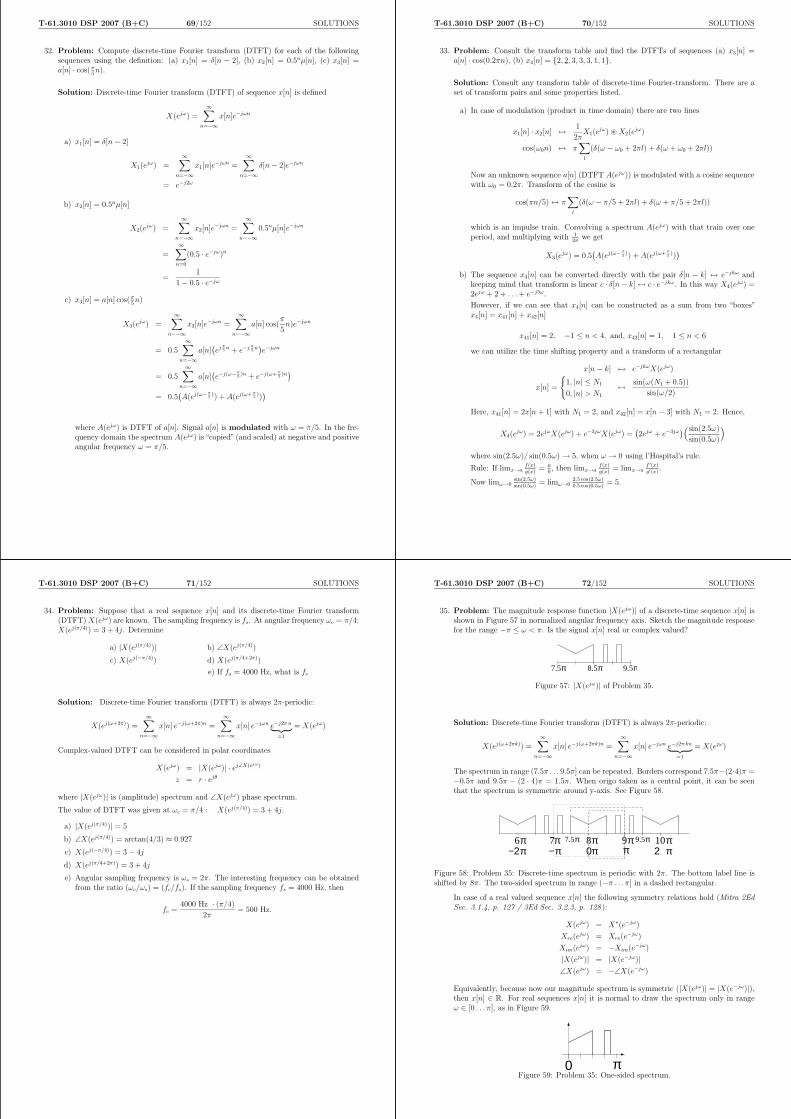
T-61.3010 DSP 2007 (B+C) 69/152 SOLUTIONS
32. Problem: Compute discrete-time Fourier transform (DTFT) for each of the followingsequences using the definition: (a) x1[n] = δ[n − 2], (b) x2[n] = 0.5nµ[n], (c) x3[n] =a[n] · cos(π
5n).
Solution: Discrete-time Fourier transform (DTFT) of sequence x[n] is defined
X(ejω) =∞∑
n=−∞
x[n]e−jωn
a) x1[n] = δ[n− 2]
X1(ejω) =
∞∑
n=−∞
x1[n]e−jωn =∞∑
n=−∞
δ[n− 2]e−jωn
= e−j2ω
b) x2[n] = 0.5nµ[n]
X2(ejω) =
∞∑
n=−∞
x2[n]e−jωn =
∞∑
n=−∞
0.5nµ[n]e−jωn
=
∞∑
n=0
(0.5 · e−jω)n
=1
1− 0.5 · e−jω
c) x3[n] = a[n] cos(π5n)
X3(ejω) =
∞∑
n=−∞
x3[n]e−jωn =∞∑
n=−∞
a[n] cos(π
5n)e−jωn
= 0.5∞∑
n=−∞
a[n](ej π
5n + e−j π
5n)e−jωn
= 0.5
∞∑
n=−∞
a[n](e−j(ω−π
5)n + e−j(ω+ π
5)n)
= 0.5(A(ej(ω−π
5)) + A(ej(ω+ π
5)))
where A(ejω) is DTFT of a[n]. Signal a[n] is modulated with ω = π/5. In the fre-quency domain the spectrum A(ejω) is “copied” (and scaled) at negative and positiveangular frequency ω = π/5.
T-61.3010 DSP 2007 (B+C) 70/152 SOLUTIONS
33. Problem: Consult the transform table and find the DTFTs of sequences (a) x3[n] =a[n] · cos(0.2πn), (b) x4[n] = 2, 2, 3, 3, 3, 1, 1.
Solution: Consult any transform table of discrete-time Fourier-transform. There are aset of transform pairs and some properties listed.
a) In case of modulation (product in time domain) there are two lines
x1[n] · x2[n] ↔ 1
2πX1(e
jω) ⊛ X2(ejω)
cos(ω0n) ↔ π∑
l
(δ(ω − ω0 + 2πl) + δ(ω + ω0 + 2πl))
Now an unknown sequence a[n] (DTFT A(ejω)) is modulated with a cosine sequencewith ω0 = 0.2π. Transform of the cosine is
cos(πn/5)↔ π∑
l
(δ(ω − π/5 + 2πl) + δ(ω + π/5 + 2πl))
which is an impulse train. Convolving a spectrum A(ejω) with that train over oneperiod, and multiplying with 1
2πwe get
X3(ejω) = 0.5
(A(ej(ω−π
5)) + A(ej(ω+ π
5)))
b) The sequence x4[n] can be converted directly with the pair δ[n − k] ↔ e−jkω andkeeping mind that transform is linear c · δ[n− k]↔ c · e−jkω. In this way X4(e
jω) =2ejω + 2 + . . . + e−j5ω.
However, if we can see that x4[n] can be constructed as a sum from two “boxes”x4[n] = x41[n] + x42[n]
x41[n] = 2, −1 ≤ n < 4, and, x42[n] = 1, 1 ≤ n < 6
we can utilize the time shifting property and a transform of a rectangular
x[n− k] ↔ e−jkωX(ejω)
x[n] =
1, |n| ≤ N1
0, |n| > N1
↔ sin(ω(N1 + 0.5))
sin(ω/2)
Here, x41[n] = 2x[n + 1] with N1 = 2, and x42[n] = x[n− 3] with N1 = 2. Hence,
X4(ejω) = 2ejωX(ejω) + e−3jωX(ejω) =
(2ejω + e−3jω
)(sin(2.5ω)
sin(0.5ω)
)
where sin(2.5ω)/ sin(0.5ω)→ 5, when ω → 0 using l’Hospital’s rule.
Rule: If limx→af(x)g(x)
= 00, then limx→a
f(x)g(x)
= limx→af ′(x)g′(x)
.
Now limω→0sin(2.5ω)sin(0.5ω)
= limω→02.5 cos(2.5ω)0.5 cos(0.5ω)
= 5.
T-61.3010 DSP 2007 (B+C) 71/152 SOLUTIONS
34. Problem: Suppose that a real sequence x[n] and its discrete-time Fourier transform(DTFT) X(ejω) are known. The sampling frequency is fs. At angular frequency ωc = π/4:X(ej(π/4)) = 3 + 4j. Determine
a) |X(ej(π/4))| b) ∠X(ej(π/4))
c) X(ej(−π/4)) d) X(ej(π/4+2π))
e) If fs = 4000 Hz, what is fc
Solution: Discrete-time Fourier transform (DTFT) is always 2π-periodic:
X(ej(ω+2π)) =∞∑
n=−∞
x[n] e−j(ω+2π)n =∞∑
n=−∞
x[n] e−jωn e−j2π n︸ ︷︷ ︸
=1
= X(ejω)
Complex-valued DTFT can be considered in polar coordinates
X(ejω) = |X(ejω)| · ej∠X(ejω)
z = r · ejθ
where |X(ejω)| is (amplitude) spectrum and ∠X(ejω) phase spectrum.
The value of DTFT was given at ωc = π/4 : X(ej(π/4)) = 3 + 4j.
a) |X(ej(π/4))| = 5
b) ∠X(ej(π/4)) = arctan(4/3) ≈ 0.927
c) X(ej(−π/4)) = 3− 4j
d) X(ej(π/4+2π)) = 3 + 4j
e) Angular sampling frequency is ωs = 2π. The interesting frequency can be obtainedfrom the ratio (ωc/ωs) = (fc/fs). If the sampling frequency fs = 4000 Hz, then
fc =4000 Hz · (π/4)
2π= 500 Hz.
T-61.3010 DSP 2007 (B+C) 72/152 SOLUTIONS
35. Problem: The magnitude response function |X(ejω)| of a discrete-time sequence x[n] isshown in Figure 57 in normalized angular frequency axis. Sketch the magnitude responsefor the range −π ≤ ω < π. Is the signal x[n] real or complex valued?
7.5π 9.5π8.5π
Figure 57: |X(ejω)| of Problem 35.
Solution: Discrete-time Fourier transform (DTFT) is always 2π-periodic:
X(ej(ω+2πk)) =
∞∑
n=−∞
x[n] e−j(ω+2πk)n =
∞∑
n=−∞
x[n] e−jωn e−j2π kn︸ ︷︷ ︸
=1
= X(ejω)
The spectrum in range (7.5π . . . 9.5π] can be repeated. Borders correspond 7.5π−(2·4)π =−0.5π and 9.5π − (2 · 4)π = 1.5π. When origo taken as a central point, it can be seenthat the spectrum is symmetric around y-axis. See Figure 58.
6 7 8 9 10π π π π π7.5π 9.5π0πππ−2 − π π2
Figure 58: Problem 35: Discrete-time spectrum is periodic with 2π. The bottom label line isshifted by 8π. The two-sided spectrum in range (−π . . . π] in a dashed rectangular.
In case of a real valued sequence x[n] the following symmetry relations hold (Mitra 2EdSec. 3.1.4, p. 127 / 3Ed Sec. 3.2.3, p. 128 ):
X(ejω) = X∗(e−jω)
Xre(ejω) = Xre(e
−jω)
Xim(ejω) = −Xim(e−jω)
|X(ejω)| = |X(e−jω)|∠X(ejω) = −∠X(e−jω)
Equivalently, because now our magnitude spectrum is symmetric (|X(ejω)| = |X(e−jω)|),then x[n] ∈ R. For real sequences x[n] it is normal to draw the spectrum only in rangeω ∈ [0 . . . π], as in Figure 59.
0 πFigure 59: Problem 35: One-sided spectrum.

T-61.3010 DSP 2007 (B+C) 73/152 SOLUTIONS
36. Problem: A LTI filter is characterized by its difference equation y[n] = 0.25x[n]+0.5x[n−1] + 0.25x[n − 2]. (a) Draw the block diagram, (b) What is the impulse response h[n],
(c) Determine the frequency response H(ejω) =P
pke−jωkP
dke−jωk , (d) Determine the amplitude
response |H(ejω)|, (e) Determine the phase response ∠H(ejω), (f) Determine the group
delay τ(ω) = −d∠H(ejω)dω
.
Solution: (Mitra 2Ed Sec. 4.2.7, 4.2.6 / 3Ed Sec. 3.8.3, 3.9.1 ) LTI system can becharacterized by a linear constant coefficient difference equation of form
∑
k
dky[n− k] =∑
k
pkx[n− k]
The corresponding frequency response can be derived by Fourier transform (ax[n− k]↔ae−jωkX(ejω)) or directly
H(ejω) =
∑pke
−jωk
∑dke−jωk
a) Draw! (You can use http://www.cis.hut.fi/Opinnot/T-61.3010/Suodin/ butthat was not in use in January 2007.)
b) As earlier explained, h[n] = 0.25δ[n] + 0.5δ[n− 1] + 0.25δ[n− 2].
c) The frequency response H can be expressed by its amplitude response |H| and theangle ∠H :
H(ejω) = |H(ejω)|ej∠H(ejω)
Now using the expression above,
H(ejω) =0.25 + 0.5e−jω + 0.25e−j2ω
1
In this particular case, when there exists a certain type of symmetry in the impulseresponse h[n] (Mitra 2Ed Sec. 4.4.3 / 3Ed Sec. 7.3 ), we may continue
H(ejω) = 0.25 + 0.5e−jω + 0.25e−j2ω
= e−jω(
0.25ejω + 0.5 + 0.25e−jω)
= e−jω(
0.5 cos(ω) + 0.5)
d) When computing values for the amplitude response in range [0 . . . π] we will get thecurve which says if the filter is lowpass / highpass / etc. |A ·B · C| = |A| · |B| · |C|.
|H(ejω)| = |e−jω|︸ ︷︷ ︸
=1
· |(
0.5 cos(ω) + 0.5)
| = |0.5 cos(ω) + 0.5|
e) Now, in this case we see that the phase response is linear. ∠(A ·B ·C) = ∠A+∠B +∠C.
∠H(ejω) = ∠e−jω + ∠(
0.5 cos(ω) + 0.5)
︸ ︷︷ ︸
=0
= −ω
f) In case of linear phase response, the group delay is constant for all frequencies. Inthis case the output sequence is delayed by 1 in the filter.
τ(ω) = − d
dω∠H(ejω) = 1
T-61.3010 DSP 2007 (B+C) 74/152 SOLUTIONS
37. Problem: Show that the periodic impulse train p(t) =∑∞
n=−∞ δ(t−nT ) can be expressedas a Fourier series p(t) = 1
T
∑∞k=−∞ ejΩT kt, where ΩT = 2π/T is the sampling angular
frequency.
Solution: Since p(t)
p(t) =∞∑
n=−∞
δ(t− nT )
is a periodic function of time t with a period T (time between samples), it can be repre-sented as Fourier series (F-series for periodic, F-transform for non-periodic signals):
p(t) =∞∑
n=−∞
cn ej(2πnt/T )
where Fourier coefficients (note, p(t) over one period T )
cn =1
T
∫
T
p(t) e−j(2πnt/T ) dt
The unit impulse function (continous-time) has properties(1)∫∞
−∞δ(t) dt = 1, and
(2)∫∞
−∞δ(t)a(t) dt = a(t)|t=0.
Therefore Fourier series coefficients are:
cn =1
T
∫ T/2
−T/2
δ(t) e−j(2πnt/T )dt =1
Te−j(2πnt/T )|t=0 =
1
T
Hence
p(t) =
∞∑
n=−∞
δ(t− nT ) =1
T
∞∑
n=−∞
ej(2πnt/T )
t n
p(t) cnT
1/T
−2
... .........
−1 0 1 2 3 4
Figure 60: Problem 37: impulse train p(t) left, and its Fourier series coefficients cn right.
T-61.3010 DSP 2007 (B+C) 75/152 SOLUTIONS
38. Problem: Impulse train in Problem 37 can be also expressed as a Fourier transformP (jΩ) = 2π
Ts
∑∞k=−∞ δ(Ω − k Ωs). Sampling can be modelled as multiplication in time
domain x[n] = xp(t) = x(t)p(t). What is Xp(jΩ) for an arbitrary input spectrum X(jΩ)?
Solution: The Fourier series of a continuous-time signal can be expressed
x(t) =∞∑
k=−∞
ak ejkΩ0t
where ak are Fourier coefficients and Ω0 is fundamental angular frequency. Fourier trans-form of a periodic signal can be written in form of
X(jΩ) =∞∑
k=−∞
2πak δ(Ω− kΩ0)
So, the impulse train p(t) of Problem 37 with all coefficients ak = 1/Ts and fundamentalangular frequency Ωs can be written as
P (jΩ) =2π
Ts
∞∑
k=−∞
δ(Ω− kΩs)
Sampling in time and frequency domain can be modeled x[n] = x(t) · p(t)↔ 12π
[X(jΩ) ⊛
P (jΩ)], which finally gives
1
2π
[P (jΩ) ⊛ X(jΩ)
]=
1
2π
∫ ∞
−∞
P (jθ)X(j(Ω− θ))dθ
=1
2π
∫ ∞
−∞
2π
Ts
∞∑
k=−∞
δ(θ − kΩs)X(j(Ω− θ))dθ
=1
Ts
∞∑
k=−∞
∫ ∞
−∞
δ(θ − kΩs)X(j(Ω− θ))dθ |∫
δ(t)x(t)dt = x(t)|t=0
=1
Ts
∞∑
k=−∞
X(j(Ω− kΩs))
In other words, the spectrum X(ejω) of the discrete-time signal x[n] can be obtainedby summing the shifted spectra X(jΩ) of the corresponding analog signal x(t). SpectraX(jΩ) are scaled by (1/Ts) and copied at every sampling (angular) frequency.
W
P(jW)
−2
... ...
0 2 4
2pi/T
W−2 0 2 4
X(jW)
W
......
(1/T) P(jW) * X(jW)
Figure 61: Problem 38: Left, an example of a spectrum P (jΩ) of an impulse train, middle, aspectrum X(jΩ) of an arbitrary signal, and their convolution in right. Notice that X(jΩ) isnot symmetric, which means that x(t) is complex-valued.
T-61.3010 DSP 2007 (B+C) 76/152 SOLUTIONS
39. Problem: Suppose that a continuous-time signal x(t) and its spectrum |X(jΩ)| in Fig-ure 62 are known. The highest frequency component in the signal is fh. The signal issampled with frequency fs, i.e. the interval between samples is Ts = 1/fs: x[n] = x(nTs).Sketch the spectrum |X(ejω)| of the discrete-time signal, when (a) fh = 0.25 fs, (b)fh = 0.5 fs, (c) fh = 0.75 fs.
hf
1
|X(jw)|
Figure 62: Spectrum X(jΩ) in Problem 39 also at page 14.
Solution: The spectrum X(jΩ) of a real analog signal is symmetric around y-axis.When sampling, the spectrum X(ejω) is 2π-periodic (sampling frequency)
x[n] = xp(nTs) = x(t)p(t) ↔ X(ejω) =1
Ts
∞∑
k=−∞
X(j(Ω− kΩs))
a) Figure 63. The highest component of x(t) is only 0.25 · fs ⇒ No aliasing.
f /2 fs sh
1
f
|X (j )|p ω
Figure 63: fh = 0.25 fs, no aliasing in Problem 39(a).
b) Figure 64. Case: Nyquist frequency, half of the sampling frequency.
1
f h
2
|X (j )|p ω
sf /2s f s f
Figure 64: fh = 0.5 fs, critical sampling in Problem 39(b).
c) Figure 65. Aliasing takes place. X(ejω) is the sum of all folded analog spectra. Thespectrum X(ejω) is depicted in Figure 65 with a thick continuous line.
X(ejω) =1
Ts
(
... + X(j(Ω− Ωs)) + X(jΩ) + X(j(Ω + Ωs)) + ...
)
1
f h
2 3
p|X (j )|
f /2s f s sfsf
ω
Figure 65: fh = 0.75 fs, aliasing in Problem 39(c).

T-61.3010 DSP 2007 (B+C) 77/152 SOLUTIONS
40. Problem: Consider a continuous-time signal x(t) = cos(2πf1t)+cos(2πf2t)+cos(2πf3t),where f1=100 Hz, f2=300 Hz and f3=750 Hz. The signal is sampled using frequency fs.Sketch the magnitude of the Fourier spectrum of x[n], when fs equals to (i) 1600 Hz (ii)800 Hz (iii) 400 Hz.
Use an ideal reconstruction lowpass filter whose cutoff frequency is fs/2 for each case.What frequency components can be found in reconstructed analog signal xr(t)?
Solution: There is a continuous-time signal
x(t) = cos(2πf1t) + cos(2πf2t) + cos(2πf3t)
Let f1 = 100 Hz, f2 = 300 Hz and f3 = 750 Hz.
It is possible directly to express the Fourier transform of a periodic signal using transformpairs (or see Page 75). In this case using Hertz
X(jf) = π ·(δ[f + 750] + δ[f + 300] + δ[f + 100] + δ[f − 100] + δ[f − 300] + δ[f − 750]
)
The signal is sampled with sampling frequency fs, (T = 1/fs).
x[n] = x(nT ) = x(n
fs
) =
(
cos(2πf1
fs
n) + cos(2πf2
fs
n) + cos(2πf3
fs
n)
)
In the frequency domain the discrete-time spectrum Gp(jΩ) can be seen as a sum of shiftedand scaled replicas of the analog spectrum Ga(jΩ) as shown in Problems 38 and 39 (Mitra2Ed Eq. 5.9, p. 302 / 3Ed Eq. 4.10, p. 174 ):
Gp(jΩ) =1
T
∞∑
k=−∞
Ga(j(Ω− kΩT ))
Alternatively, sampling can be considered as flipping the analog spectrum around eachhalf of the sampling frequency down to the band 0 . . . fs/2.
Reconstruction means converting a digital sequence back to analog signal. An ideallowpass filter with the passband up to half of the sampling frequency is used. Whenreconstructing signals we can only observe frequencies up to Nyquist frequency.1 If thereare frequencies over the Nyquist frequency in the original signal, those frequencies arealiased into low frequencies.
In this problem X(jΩ) is sampled with three different sampling frequencies fs of 1600 Hz,800 Hz and 400 Hz, The Nyquist frequency is the half of the sampling frequency fs/2,800 Hz, 400 Hz, and 200 Hz, respectively. Let fm (in this case 750 Hz) be the biggestfrequency found in the input signal. If the sampling frequency is less than 2fm = 1500Hz, then there will be aliasing.
In the following figures for i, ii and iii, the scale and magnitude values for aliased frequen-cies are not exactly correct. Phase shifts in input signal cause that a pure addition ofmagnitudes will not hold. (The sum of two cosines with same frequency and phase shiftof π is zero. However, in practice, this is rarely significant.)
i) fs = 1600 Hz, highest frequency component fm = 750 Hz. The inequality 1600 >2 · 750 holds, hence, there is no aliasing. All three frequencies can be recovered. SeeFigure 66.
1There is variation in using “Nyqvist frequency” in the literature. It is either (1) half of the samplingfrequency (Mitra 2Ed p. 302 / 3Ed p. 174 ) or (2) the highest frequency in the signal (Mitra 2Ed p. 304 / 3Edp. 176 ). The first one is much more common. The reader should not confuse with this.
T-61.3010 DSP 2007 (B+C) 78/152 SOLUTIONS
a
w (f, Hz)200 600
1000 w (f, Hz)600200
|X (jw)|
p|X (jw)|
fs/2
0 0.002 0.004 0.006 0.008 0.01 0.012 0.014 0.016 0.018 0.02
−2
0
2
x(t)
fs = 1600 Hz
0 0.002 0.004 0.006 0.008 0.01 0.012 0.014 0.016 0.018 0.02
−2
0
2
x(t)
.p(t
)
0 0.002 0.004 0.006 0.008 0.01 0.012 0.014 0.016 0.018 0.02
−2
0
2
x[n]
0 0.002 0.004 0.006 0.008 0.01 0.012 0.014 0.016 0.018 0.02
−2
0
2
reco
nst.
0 0.002 0.004 0.006 0.008 0.01 0.012 0.014 0.016 0.018 0.02
−2
0
2
x r(t)
Figure 66: Sampling in Problem 40(i) with sampling frequency 1600 Hz: original analog spec-trum X(jΩ) (left top), and spectrum X(ejω) of the discrete-time signal (left bottom). Timedomain view (right), top down x(t), sampling x(t) · p(t) sampled sequence x[n] to be processedwith DSP, reconstruction, and reconstructed continuous-time signal xr(t). Again, in this caseno aliasing, i.e. x(t) ≡ xr(t).
ii) fs = 800 Hz, highest frequency component fm = 750 Hz. The inequality 800 > 2 ·750does not hold, hence, there is aliasing. All frequencies over 400 Hz are missed (750 Hzin this case); they cannot be observed. There is a new alias component at frequency50 Hz. See Figure 67.
a|X (jw)|
w (f, Hz)
311
33
3 11 22 33p
1000 w (f, Hz)600200
600200
1
|X (jw)|2 2
2 21
/2sf
0 0.002 0.004 0.006 0.008 0.01 0.012 0.014 0.016 0.018 0.02
−2
0
2
x(t)
fs = 800 Hz
0 0.002 0.004 0.006 0.008 0.01 0.012 0.014 0.016 0.018 0.02
−2
0
2
x(t)
.p(t
)
0 0.002 0.004 0.006 0.008 0.01 0.012 0.014 0.016 0.018 0.02
−2
0
2
x[n]
0 0.002 0.004 0.006 0.008 0.01 0.012 0.014 0.016 0.018 0.02
−2
0
2
reco
nst.
0 0.002 0.004 0.006 0.008 0.01 0.012 0.014 0.016 0.018 0.02
−2
0
2
x r(t)
Figure 67: Sampling in Problem 40(ii) with sampling frequency 800 Hz. Aliasing occurs,x(t) 6= xr(t), compare the top and bottom axis in the figure right.
Before going further, there is a short demonstration on the aliasing signal componentx3(t) (fi = 750 Hz) of the signal x(t) in Figure 68. The figures are depicted intime-domain: (a) original x(t) with period T = 1/f = (1/750) = 1.333 ms, (b)samples x[n] using interval Ts = 1/fs = (1/800) = 1.250 ms, (c) reconstructedsignal x3r(t), whose period Tr = (1/50) = 20 ms. The same aliasing effect can beshown using the cosine function, which is 2π-periodic (cos(ωn) ≡ cos(ωn + 2π)) andeven (cos(−ωn) ≡ cos(ωn)). The highest component x3(t) of 750 Hz aliases in thesampling and reconstructing process to 50 Hz:
x3(t) = cos(2π 750t) | original: 750 Hz
x3[n] = x3(n/fs) = cos(2π(750/800)n) = cos(2π(750/800)n− 2πn) | 2π-periodicity
= cos(2π(−50/800)n) = cos(2π(50/800)n) | even function
x3r(t) = cos(2π 50t) | reconstructed: 50 Hz
T-61.3010 DSP 2007 (B+C) 79/152 SOLUTIONS
−1
0
1T=(1/750)=1.33ms
x 3(t)
−1
0
1
x[n]
0 2 4 6 8 10 12 14 16 18 20−1
0
1
t (ms)
x 3r(t
)
Figure 68: Demonstration of aliasing of a single cosine in Problem 40(ii).
iii) fs = 400 Hz, highest frequency component fm = 750 Hz. The inequality 400 > 2 ·750does not hold, hence, there is aliasing. All frequencies over 200 Hz are missed (300and 750 Hz). There are new alias components at frequencies 50 and 100 Hz. SeeFigure 69.
cos(2π 750400
n) = cos(2π 750400
n− 4πn) = cos(2π−50400
n) = cos(2π 50400
n)
cos(2π 300400
n) = cos(2π 300400
n− 2πn) = cos(2π−100400
n) = cos(2π 100400
n)
233
2
33
1
2
133
2
11
2
200 w (f, Hz)
a|X (jw)|
600
21 1
1000 w (f, Hz)600200
p|X (jw)|/2sf
0 0.002 0.004 0.006 0.008 0.01 0.012 0.014 0.016 0.018 0.02
−2
0
2
x(t)
fs = 400 Hz
0 0.002 0.004 0.006 0.008 0.01 0.012 0.014 0.016 0.018 0.02
−2
0
2
x(t)
.p(t
)
0 0.002 0.004 0.006 0.008 0.01 0.012 0.014 0.016 0.018 0.02
−2
0
2
x[n]
0 0.002 0.004 0.006 0.008 0.01 0.012 0.014 0.016 0.018 0.02
−2
0
2
reco
nst.
0 0.002 0.004 0.006 0.008 0.01 0.012 0.014 0.016 0.018 0.02
−2
0
2
x r(t)
Figure 69: Sampling in Problem 40(iii) with sampling frequency 400 Hz. Aliasing occurs again,x(t) 6= xr(t).
After ideal reconstruction (x[n]→ xr(t)) there are the following components left:
(i) original 100, 300, 750 Hz.
(ii) original 100, 300 Hz, and an alias 50 Hz.
(iii) original 100 Hz, and aliases 50, 100 Hz.
There is a sampling (aliasing) demo in the demo section in the course web pages http:
//www.cis.hut.fi/Opinnot/T-61.3010/ Demo can also be loaded to Matlab.
T-61.3010 DSP 2007 (B+C) 80/152 SOLUTIONS
41. Problem: Real analog signal x(t), whose spectrum |X(jΩ)| is drawn in Figure 70, issampled with sampling frequency fs = 8000 Hz into a sequence x[n].
(a) Smallest sufficient sampling frequency? (b) How many samples in x[n]? (c) Sketch thespectrum |X(ejω)|. (d) Filter with LTI in Figure 70. Output y[n] reconstructed (ideally)to continuous-time yr(t). Sketch the spectrum |Yr(jΩ)|.
|X(j )|Ω
84 f (kHz) −1 −0.5 0 0.5 1−1
−0.5
0
0.5
1
21
Figure 70: Problem 41: Spectrum left. Pole-zero plot right.
Solution: The Shannon (Nyqvist) sampling theorem is discussed in (Mitra 2Ed Sec. 5.2,p. 302 / 3Ed Sec. 4.2, p. 176 ).
a) The highest frequency component in the analog signal is fh = 9 kHz. Thus therequired sampling frequency would be fT = 2fh = 18 kHz.
b) The sampling frequency is 8 kHz, which means that there are 8000 samples eachsecond. Now
x
0.2 s=
8000
1 s
gives 1600 samples for 0.2 seconds.
c) Due to too low sampling frequency aliasing occurs. All frequency components abovefT /2 = 4 kHz are aliased into low frequencies between 0 . . . 4 kHz. Sampling in thefrequency domain can be considered as copying the original analog spectrum at eachmultiple of the sampling frequency (Mitra 2Ed Eq. 5.9, p. 302 / 3Ed Eq. 4.10, p.174 )
Gdiscrete(jΩ) =1
T
∞∑
k=−∞
Ganalog(j(Ω + kΩT ))
Here we show another way of finding the discrete-time spectrum. If the analog signalis real-valued and the amplitude spectrum therefore symmetric around y-axis, thesampling can also be thought as flipping each fT /2 wide band of the analog spectrumdownwards into the fundamental range 0 . . . fT /2.
First, divide the spectrum to a set of bands, whose width is fT /2. In this case wehave B0 = [0 . . . 4000) Hz, B1 = [4000 . . .8000) Hz, and B2 = [8000 . . . 12000) Hz.
Flip the band B2 around 8000 Hz (mirror) down to B1. Spectral components of B1
and the mirrored B2 are summed together. See Figure 71 left top. Note! Sinusoidalcomponents with opposite phase (180) vanish: sin(ωB2→B1n) + sin(ωB1n + π) = 0,if ωB2→B1 = ωB1. However, in practice this is not usual, and the addition operationcan be considered as a good approximation.
Finally, the band B1 is mirrored around 4000 Hz down to the fundamental band B0,and the spectral components are summed together. See Figure 71 left bottom and

T-61.3010 DSP 2007 (B+C) 81/152 SOLUTIONS
84 12
B B10
84 12
B B B10 2 |X(e )|jω
84 f (kHz)
|X(j )|Ω
Figure 71: Problem 41: (a) Two steps when mirroring spectral bands down to the fundamentalband 0 . . . 4 kHz. (b) Discrete-time spectrum |X(ejω)|. Scaling factors are not taken intoaccount.
the final result in Figure 71 right. Scaling factors (height) are not taken into accounthere.
d) If pole-zero plots are not familiar, consult (Mitra 2Ed Sec. 4.3.4 / 3Ed Sec. 6.7.4 )or Problem 46, p. 88.
The sampling frequency is 8 kHz. In the pole-zero plot the whole circle 2π corre-sponds 8 kHz. The upper part of the circle from ω = 0 to ω = π is 0 . . . 4 kHz.There are zeros on the unit circle from 2 . . . 4 kHz. Hence, the filter is a lowpassfilter, whose cut-off frequency is about at 2 kHz.
The discrete-time signal x[n] is filtered with a lowpass filter. Here we use a roughapproximation of the filter depicted with a pole-zero plot, an ideal lowpass filterH(ejω) with cut-off at 2 kHz. The spectrum of filtered signal is Y (ejω) = H(ejω) ·X(ejω) shown in Figure 72(a). Note! Filter with zeros like in Figure 70 is not ideal.You can plot its real amplitude response using Matlab.
After reconstructing ideally (ideal lowpass filter with cut-off at fT /2) the sequencey[n] back to analog yr(t), the spectrum |Yr(jΩ)| is plotted in in Figure 72(b).
|Y(e )|jω
84 f (kHz)
Ω|Y(j )|
84 f (kHz)12 20
Figure 72: Problem 41: (a) Spectra |Y (ejω)| and (b) |Yr(jΩ)|. Discrete-time spectrum |Y (ejω)|is periodic every 2π (or every fT ), wheras continuous-time spectrum |Yr(jΩ)| is not periodic.Scaling factors are not taken into account.
T-61.3010 DSP 2007 (B+C) 82/152 SOLUTIONS
42. Problem: Sketch specifications and compute the order for an anti-aliasing Butterworthfilter with fs = 8 kHz, interesting band 0 . . . 2 kHz, and minimum stopband attenuation50 dB.
Solution: An anti-aliasing filter is an analog lowpass filter used in order to removecomponents, which cause aliasing when sampling (Mitra 2Ed Sec. 5.6 / 3Ed Sec. 4.6 ).Consider an analog signal x(t) and its spectrum X(jΩ) depicted in Figure 73.
f
|X|
kHz8642Figure 73: Spectrum X(jΩ) in Problem 42.
In the following, notations of (Mitra 2Ed Fig. 5.28 / 3Ed Fig. 4.34 ) are used, Ωp forpassband edge frequency, Ω0 = ΩT −Ωp for stopband edge frequency, and ΩT for samplingfrequency. Now that the interesting band stops at Ωp = 2 kHz and the sampling frequencyis ΩT = 8 kHz, we can set the edge frequency for the stopband to be at Ω0 = (8− 2) = 6kHz (see Figure 74). After sampling there will be aliasing components in 2 . . . 4 kHz, butwe are not interested in them, i.e. we use digital filtering for that band.
f
|X|
kHz8642
Figure 74: Problem 42: Spectrum X(jΩ), specifications for a LP filter (dashed line), frequencycomponents that would alias in 0 . . . 2 kHz without anti-aliasing filtering (gray).
When the specifications are not so tight as they normally (cut-off at 4 kHz) are, also theorder of the anti-aliasing filter is lower. The design of the anti-aliasing filter can be madeeven easier by increasing sampling frequency with analog circuits (order of anti-aliasingfilter decreases), and afterwards decrease sampling frequency using multirate techniques(Mitra 2Ed Sec. 10 / 3Ed Sec. 13 ).
Calculations using (Mitra 2Ed Table 5.1 / 3Ed Table 4.1 ) or Table 7: Ω0/Ωp = 3→ N =⌈50/9.54⌉ = 6. Note that if the passband ended at 2 kHz and the stopband started at 4kHz, the required order of the filter would be 10.
Ω0 = 2Ωp 3Ωp 4Ωp
Attenuation (dB) 6.02N 9.54N 12.04NΩT = 3Ωp 4Ωp 5Ωp
Table 7: Approximate minimum stopband attenuation of a Butterworth lowpass filter, (Mitra2Ed Table 5.1, p. 336 / 3Ed Table 4.1, p. 210 ). See the text in Problem 42 for details.
T-61.3010 DSP 2007 (B+C) 83/152 SOLUTIONS
43. Problem: The exponent term in DFT/IDFT is commonly written WN = e−j2π/N .
a) Compute and draw in complex plane values of W k3
b) Compute 3-DFT for the sequence x[n] = 1, 3, 2.
Solution: Discrete Fourier transform (DFT), left, and Inverse Fourier transform (IDFT),right, using N points are defined
X[k] =N−1∑
n=0
x[n]W knN x[n] =
1
N
N−1∑
k=0
X[k]W−knN , WN = e−
j2πN
a) WN = e−j2πN , now N = 3.
W 03 = e−
j2π3
·0 = 1
W 13 = e−
j2π3
·1 = −0.5−√
3
2j
W 23 = e−
j2π3
·2 = −0.5 +
√3
2j
Notice that the exponent in W defines the angle jumpin clockwise. What are the values of W kn
3 , when k =0 . . . 2 and n = 0 . . . 2?. For example, k = 1, n = 2,we get W 1·2
3 = W 23 . Specially, W 2·2
3 = W 43 = e−
j2π3
·4 =
e−j2π3
·3︸ ︷︷ ︸
=1
·e− j2π3
·1 = W 13 .
k, n 0 1 2
0 W 03 W 0
3 W 03
1 W 03 W 1
3 W 23
2 W 03 W 2
3 W 13
−1 −0.5 0 0.5 1
−1
−0.5
0
0.5
1
Problem 3a. W3 = e−j 2 π / 3
W30
W31
W32
b) The sequence x[n] = 1, 3, 2 is of length 3.
X[0] =
2∑
n=0
x[n]W 0·n
= 1 + 3 + 2 = 6
X[1] =
2∑
n=0
x[n]W 1·n
= 1 ·W 0 + 3 ·W 1 + 2 ·W 2
= 1 + (−1.5− 3√
3
2j) + (−1 +
2√
3
2j) = −1.5−
√3
2j
X[2] =
2∑
n=0
x[n]W 2·n
= 1 ·W 0 + 3 ·W 2 + 2 ·W 4
= 1 + (−1.5 +3√
3
2j) + (−1− 2
√3
2j) = −1.5 +
√3
2j
Remark. Notice that
T-61.3010 DSP 2007 (B+C) 84/152 SOLUTIONS
– DFT is discrete in frequency domain (DTFT is continuous)
– N-point DFT of a real signal is (very often) complex
– if N-point DFT is real-valued then x[n] has to be “symmetric”
– each value of X[k] is a dot product of x[n] and W with some constant anglejump (nk)
– X[0] is the sum of values of x[n] (DC-component)
– values of X[k] are N-periodic: X[k] = X[k + N ] = X[k + 2N ] = . . .
– absolute values (amplitude spectrum) are even |X[1]| = |X[−1]|– angle values are odd ∠X[1] = −∠X[−1]
Discrete Fourier transform is a linear operation. It can be calculated in matrix formas (Mitra 2Ed Sec. 3.2.2 / 3Ed Sec. 5.2.2 )
X = DNx
where X is a column vector of the N frequency-domain DFT samples, x is a columnvector of N time-domain input samples, and DN is the N ×N DFT matrix (dftmtxin Matlab)
X = [X[0] X[1] . . . X[N − 1]]T
x = [x[0] x[1] . . . x[N − 1]]T
DN =
1 1 1 . . . 11 W 1
N W 2N . . . W N−1
N
1 W 2N W 4
N . . . W2(N−1)N
......
.... . .
...
1 W N−1N W
2(N−1)N . . . W
(N−1)(N−1)N
In this problem dftmtx gives as expected
D3 =
1.0000 1.0000 1.00001.0000 −0.5000− 0.8660i −0.5000 + 0.8660i1.0000 −0.5000 + 0.8660i −0.5000− 0.8660i
In the inverse DFT x = D−1N X the matrix D−1
N is
D−1N =
1
N
1 1 1 . . . 1
1 W−1N W−2
N . . . W−(N−1)N
1 W−2N W−4
N . . . W−2(N−1)N
......
.... . .
...
1 W−(N−1)N W
−2(N−1)N . . . W
−(N−1)(N−1)N
It can be seen that D−1N = (1/N)D∗
N .
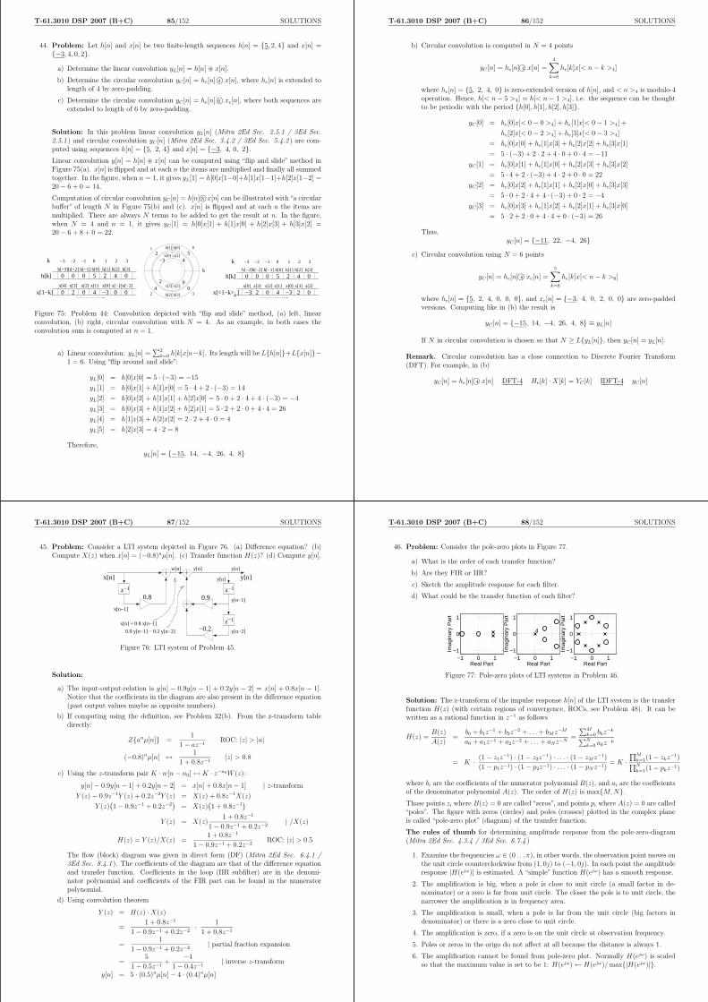
T-61.3010 DSP 2007 (B+C) 85/152 SOLUTIONS
44. Problem: Let h[n] and x[n] be two finite-length sequences h[n] = 5, 2, 4 and x[n] =−3, 4, 0, 2.
a) Determine the linear convolution yL[n] = h[n] ⊛ x[n].
b) Determine the circular convolution yC[n] = he[n] 4© x[n], where he[n] is extended tolength of 4 by zero-padding.
c) Determine the circular convolution yC [n] = he[n] 6© xe[n], where both sequences areextended to length of 6 by zero-padding.
Solution: In this problem linear convolution yL[n] (Mitra 2Ed Sec. 2.5.1 / 3Ed Sec.2.5.1 ) and circular convolution yC[n] (Mitra 2Ed Sec. 3.4.2 / 3Ed Sec. 5.4.2 ) are com-puted using sequences h[n] = 5, 2, 4 and x[n] = −3, 4, 0, 2.Linear convolution y[n] = h[n] ⊛ x[n] can be computed using “flip and slide” method inFigure 75(a). x[n] is flipped and at each n the items are multiplied and finally all summedtogether. In the figure, when n = 1, it gives yL[1] = h[0]x[1−0]+h[1]x[1−1]+h[2]x[1−2] =20− 6 + 0 = 14.
Computation of circular convolution yC [n] = h[n] N©x[n] can be illustrated with “a circularbuffer” of length N in Figure 75(b) and (c). x[n] is flipped and at each n the items aremultiplied. There are always N terms to be added to get the result at n. In the figure,when N = 4 and n = 1, it gives yC [1] = h[0]x[1] + h[1]x[0] + h[2]x[3] + h[3]x[2] =20− 6 + 8 + 0 = 22.
−3k −2 −1 0 1 2 3
x[1−k] 4 −3020 00
h[k] 5 2 4000 0h[0] h[1] h[2]h[−1]h[−2]h[−3] h[3]
x[0] x[−2]x[−1]x[1]x[2]x[3]x[4]
52
4 0
01
32
4−3x[1]x[0]
x[3]2 0
x[2]
h[2] h[3]
h[1] h[0]
kh[k] 5 2 4000 0
h[0] h[1] h[2]h[−1]h[−2]h[−3] h[3]
x[0] x[2]x[3]x[1]x[2]x[3]x[0]
4 −302−3 02x[<1−k> ]
−3k −2 −1 0 1 2 3
4
Figure 75: Problem 44: Convolution depicted with “flip and slide” method, (a) left, linearconvolution, (b) right, circular convolution with N = 4. As an example, in both cases theconvolution sum is computed at n = 1.
a) Linear convolution: yL[n] =∑2
k=0 h[k]x[n−k]. Its length will be Lh[n]+Lx[n]−1 = 6. Using “flip around and slide”:
yL[0] = h[0]x[0] = 5 · (−3) = −15
yL[1] = h[0]x[1] + h[1]x[0] = 5 · 4 + 2 · (−3) = 14
yL[2] = h[0]x[2] + h[1]x[1] + h[2]x[0] = 5 · 0 + 2 · 4 + 4 · (−3) = −4
yL[3] = h[0]x[3] + h[1]x[2] + h[2]x[1] = 5 · 2 + 2 · 0 + 4 · 4 = 26
yL[4] = h[1]x[3] + h[2]x[2] = 2 · 2 + 4 · 0 = 4
yL[5] = h[2]x[3] = 4 · 2 = 8
Therefore,yL[n] = −15, 14, −4, 26, 4, 8
T-61.3010 DSP 2007 (B+C) 86/152 SOLUTIONS
b) Circular convolution is computed in N = 4 points
yC[n] = he[n] 4© x[n] =
3∑
k=0
he[k]x[< n− k >4]
where he[n] = 5, 2, 4, 0 is zero-extended version of h[n], and < n >4 is modulo-4operation. Hence, h[< n− 5 >4] = h[< n− 1 >4], i.e. the sequence can be thoughtto be periodic with the period h[0], h[1], h[2], h[3].
yC[0] = he[0]x[< 0− 0 >4] + he[1]x[< 0− 1 >4] +
he[2]x[< 0− 2 >4] + he[3]x[< 0− 3 >4]
= he[0]x[0] + he[1]x[3] + he[2]x[2] + he[3]x[1]
= 5 · (−3) + 2 · 2 + 4 · 0 + 0 · 4 = −11
yC[1] = he[0]x[1] + he[1]x[0] + he[2]x[3] + he[3]x[2]
= 5 · 4 + 2 · (−3) + 4 · 2 + 0 · 0 = 22
yC[2] = he[0]x[2] + he[1]x[1] + he[2]x[0] + he[3]x[3]
= 5 · 0 + 2 · 4 + 4 · (−3) + 0 · 2 = −4
yC[3] = he[0]x[3] + he[1]x[2] + he[2]x[1] + he[3]x[0]
= 5 · 2 + 2 · 0 + 4 · 4 + 0 · (−3) = 26
Thus,yC[n] = −11, 22, −4, 26
c) Circular convolution using N = 6 points
yC [n] = he[n] 6© xe[n] =
5∑
k=0
he[k]x[< n− k >6]
where he[n] = 5, 2, 4, 0, 0, 0, and xe[n] = −3, 4, 0, 2, 0, 0 are zero-paddedversions. Computing like in (b) the result is
yC [n] = −15, 14, −4, 26, 4, 8 ≡ yL[n]
If N in circular convolution is chosen so that N ≥ LyL[n], then yC [n] = yL[n].
Remark. Circular convolution has a close connection to Discrete Fourier Transform(DFT). For example, in (b)
yC[n] = he[n] 4© x[n] DFT-4−−−−→ He[k] ·X[k] = YC[k] IDFT-4−−−−−→ yC[n]
T-61.3010 DSP 2007 (B+C) 87/152 SOLUTIONS
45. Problem: Consider a LTI system depicted in Figure 76. (a) Difference equation? (b)Compute X(z) when x[n] = (−0.8)nµ[n]. (c) Transfer function H(z)? (d) Compute y[n].
z−1 z−1
0.8
x[n] y[n]
z−1
−0.2
0.9
x[n−1]
y[n−1]
y[n−2]
y[n] y[n]
y[n]
x[n] + 0.8 x[n−1]
0.9 y[n−1] − 0.2 y[n−2]
w[n]
Figure 76: LTI system of Problem 45.
Solution:
a) The input-output-relation is y[n] − 0.9y[n − 1] + 0.2y[n − 2] = x[n] + 0.8x[n − 1].Notice that the coefficients in the diagram are also present in the difference equation(past output values maybe as opposite numbers).
b) If computing using the definition, see Problem 32(b). From the z-transform tabledirectly:
Zanµ[n] =1
1− az−1ROC: |z| > |a|
(−0.8)nµ[n] ↔ 1
1 + 0.8z−1|z| > 0.8
c) Using the z-transform pair K · w[n− n0]↔ K · z−n0W (z):
y[n]− 0.9y[n− 1] + 0.2y[n− 2] = x[n] + 0.8x[n− 1] | z-transform
Y (z)− 0.9z−1Y (z) + 0.2z−2Y (z) = X(z) + 0.8z−1X(z)
Y (z)(1− 0.9z−1 + 0.2z−2
)= X(z)
(1 + 0.8z−1
)
Y (z) = X(z)1 + 0.8z−1
1− 0.9z−1 + 0.2z−2| /X(z)
H(z) = Y (z)/X(z) =1 + 0.8z−1
1− 0.9z−1 + 0.2z−2ROC: |z| > 0.5
The flow (block) diagram was given in direct form (DF) (Mitra 2Ed Sec. 6.4.1 /3Ed Sec. 8.4.1 ). The coefficients of the diagram are that of the difference equationand transfer function. Coefficients in the loop (IIR subfilter) are in the denomi-nator polynomial and coefficients of the FIR part can be found in the numeratorpolynomial.
d) Using convolution theorem
Y (z) = H(z) ·X(z)
=1 + 0.8z−1
1− 0.9z−1 + 0.2z−2· 1
1 + 0.8z−1
=1
1− 0.9z−1 + 0.2z−2| partial fraction expansion
=5
1− 0.5z−1+
−4
1− 0.4z−1| inverse z-transform
y[n] = 5 · (0.5)nµ[n]− 4 · (0.4)nµ[n]
T-61.3010 DSP 2007 (B+C) 88/152 SOLUTIONS
46. Problem: Consider the pole-zero plots in Figure 77.
a) What is the order of each transfer function?
b) Are they FIR or IIR?
c) Sketch the amplitude response for each filter.
d) What could be the transfer function of each filter?
−1 0 1−1
0
1
Real Part
Imag
inar
y P
art
−1 0 1−1
0
1
Real Part
Imag
inar
y P
art
4
−1 0 1−1
0
1
Real Part
Imag
inar
y P
art
Figure 77: Pole-zero plots of LTI systems in Problem 46.
Solution: The z-transform of the impulse response h[n] of the LTI system is the transferfunction H(z) (with certain regions of convergence, ROCs, see Problem 48). It can bewritten as a rational function in z−1 as follows
H(z) =B(z)
A(z)=
b0 + b1z−1 + b2z
−2 + . . . + bMz−M
a0 + a1z−1 + a2z−2 + . . . + aNz−N=
∑Mk=0 bkz
−k
∑Nk=0 akz−k
= K · (1− z1z−1) · (1− z2z
−1) · . . . · (1− zMz−1)
(1− p1z−1) · (1− p2z−1) · . . . · (1− pNz−1)= K ·
∏Mk=1(1− zkz
−1)∏N
k=1(1− pkz−1)
where bi are the coefficients of the numerator polynomial B(z), and ai are the coefficientsof the denominator polynomial A(z). The order of H(z) is maxM, N.Those points zi where B(z) = 0 are called “zeros”, and points pi where A(z) = 0 are called“poles”. The figure with zeros (circles) and poles (crosses) plotted in the complex planeis called “pole-zero plot” (diagram) of the transfer function.
The rules of thumb for determining amplitude response from the pole-zero-diagram(Mitra 2Ed Sec. 4.3.4 / 3Ed Sec. 6.7.4 )
1. Examine the frequencies ω ∈ (0 . . . π), in other words, the observation point moves onthe unit circle counterclockwise from (1, 0j) to (−1, 0j). In each point the amplituderesponse |H(ejω)| is estimated. A “simple” function H(ejω) has a smooth response.
2. The amplification is big, when a pole is close to unit circle (a small factor in de-nominator) or a zero is far from unit circle. The closer the pole is to unit circle, thenarrower the amplification is in frequency area.
3. The amplification is small, when a pole is far from the unit circle (big factors indenominator) or there is a zero close to unit circle.
4. The amplification is zero, if a zero is on the unit circle at observation frequency.
5. Poles or zeros in the origo do not affect at all because the distance is always 1.
6. The amplification cannot be found from pole-zero plot. Normally H(ejω) is scaledso that the maximum value is set to be 1: H(ejω)← H(ejω)/ max|H(ejω)|.

T-61.3010 DSP 2007 (B+C) 89/152 SOLUTIONS
a) The order is the maximum of the number of poles or zeros (not in origo).
So, (i) 2 poles, 1 zero: 2nd order; (ii) 4 zeros: 4th order; (iii) 6 poles, 6 zeros: 6thorder.
Note, in analog H(s) there are only poles, but in digital H(z) there can be bothpoles and zeros.
b) If there is any pole (cross in the graph) outside the origo, it means that there is atleast first-order polynomial in the denominator in H(z)⇔ there is a feedback in thesystem ⇔ IIR.
Hence, (i) IIR; (ii) FIR; (iii) IIR.
c) The analysis with graphs is done below for each case separately.
Shortly, (i) lowpass with narrow passband; (ii) highpass; (iii) a comb filter.
d) The transfer function can be constructed from zeros zi and poles pi
H(z) = K ·∏M
k=1(1− zkz−1)
∏Nk=1(1− pkz−1)
However, the scaling factor K cannot be seen from the pole-zero-plot. Therefore Kis set so that max|H(ejω)| = 1.
Next, a closer look at (c) and (d) is given for each filter.
i) Without computing any exact values of the amplitude response, it is possible toapproximate it by looking at the positions of zeros and poles. The angular frequencygets values from 0 to π, and the observation is done on a unit circle counterclockwise.
Poles are close to unit circle at ω = ±π/30 in Figure 78(a). Therefore the amplituderesponse gets the maximum approximately at that frequency and the filter is lowpasstype, see the sketch in Figure 78(b). The closer the poles are the unit circle, thenarrower the maximum area is. The value at ω = π is zero.
In this case the exact locations of poles and zeros were known (z1 = −1, p1 =0.8950 + 0.0947i, p2 = 0.8950 − 0.0947i). The actual transfer function is H(z) =K · (1 + z−1)/(1 − 1.79z−1 + 0.81z−2) from which the actual frequency response isreceived by z ← ejω. Some values in range 0 . . . π are computed below, and K ischosen so that the maximum of |H(z)| is one. Figures are plotted using Matlab inboth linear scale and in logarithmic scale in Figure 78(c) and (d), respectively.
ω H(ejω) |H(ejω)| ω H(ejω) |H(ejω)|0 1 1 3π/4 −.0008 + .0023j .0025
π/4 −.0277 + .0210j .0348 π 0 0π/2 −.0049 + .0061j .0078
ii) There are four zeros in Figure 79(left). At ω ≈ π/6 the zeros are closest to theobservation point, and the minimum of the response is probably reached (bandstop).At ω = π the zeros are much further away than at ω = 0, so the attenuation is muchstronger at low frequencies (highpass). Notice that |H(ej0)| 6= 0, because there isnot a zero on the unit circle at ω = 0. The filter can be a highpass or bandstop FIRfilter.
Actually, H(z) = 1− 3.753z−1 + 5.694z−2 − 3.753z−3 + z−4. Filter coefficients havea certain symmetry as well as the zeros lie in a certain symmetry, which implies alinear-phase filter, see Problem 49. The minimum of |H(ejω)| ≈ 0.0114 (scaled) atω ≈ 0.11π, which is different from π/6 estimated earlier. All “zero vectors” affect tothe response, see the remark text below.
T-61.3010 DSP 2007 (B+C) 90/152 SOLUTIONS
−1 0 1
−1
−0.5
0
0.5
1
Real Part
Imag
inar
y P
art
ππ/2
|H(e^jw)|
1
00 0.5 1
0
0.2
0.4
0.6
0.8
1|H
1(ej ω)|
ω * π0 0.5 1
−100
−80
−60
−40
−20
0
20 log10
(|H1(ej ω)|)
dB
ω * π
Figure 78: Problem 46(i): (a) Pole-zero-diagram, (b) an example of approximated amplituderesponse, (c) actual amplitude response |H1(e
jω)| in linear scale, (d) actual amplitude response|H1(e
jω)| in decibels.
iii) Zeros are on the unit circle at uniform invervals forcing the amplification drop downto zero, see Figure 79(right). This type of periodic filter is often called a comb filter.The maximum is scaled to one. Note that all poles and zeros affect, so that if therewere not exactly same intervals between poles and zeros, the amplitude responsewould also turn out to be non-symmetric.
−1 0 1
−1
−0.5
0
0.5
1
4
Real Part
Imag
inar
y P
art
Problem 2 (ii)
0 0.5 1
0
0.5
1
ω * π
|H2(ej ω)|
−1 0 1
−1
−0.5
0
0.5
1
Real Part
Imag
inar
y P
art
Problem 2 (iii)
0 0.5 1
0
0.5
1
ω * π
|H3(ej ω)|
Figure 79: Problem 46(ii),(iii): Pole-zero-diagram and corresponding amplitude response of|H2(e
jω)| left, and |H3(ejω)| right.
Remark. Determining amplitude response from the pole-zero-diagram, theory in back-ground.
Any transfer function H(z) can be expressed in form of
H(z) =|p0||d0|
(1− z1 z−1)(1− z2 z−1)...(1− zM z−1)
(1− p1 z−1)(1− p2 z−1)...(1− pN z−1)
In order to achieve this, all zeros (zi) and poles (pi) of H(z) has to be computed. Zerosare the roots of the numerator polynomial and poles are the roots of the denominatorpolynomial. Numerator part is “FIR part” (always stable, y[n] depends only on values ofx[n− ki]), denominator is “IIR part” (feedback, in order to compute y[n] some old valuesof it has to be used).
Frequency response is the transfer function computed on unit circle, i.e. substitutionz = ejω:
H(ejω) =|p0||d0|
(1− z1 e−jω)(1− z2 e−jω)...(1− zM e−jω)
(1− p1 e−jω)(1− p2 e−jω)...(1− pN e−jω)
We are interested in amplitude response |H(ejω)|. Because the expression is in a productform, the absolute value of |H(ejω)| can be computed with its first order blocks. LetK = |p0|/|d0|, Bi be the length of a first order block in numerator polynomial, and Ai the
T-61.3010 DSP 2007 (B+C) 91/152 SOLUTIONS
length of a first order block in denominator polynomial:
|H(ejω)| = K ·
B1︷ ︸︸ ︷
|(1− z1 e−jω)|B2
︷ ︸︸ ︷
|(1− z2 e−jω)| . . .BM
︷ ︸︸ ︷
|(1− zM e−jω)||(1− p1 e−jω)|︸ ︷︷ ︸
A1
|(1− p2 e−jω)|︸ ︷︷ ︸
A2
. . . |(1− pN e−jω)|︸ ︷︷ ︸
AN
= K ·∏M
k=1 Bk∏N
k=1 Ak
The frequency axis lies on the unit circle from ω = 0, which is a complex point ejω|ω=0 = 1to ω = π, which is situated at ejω|ω=π = −1. The observation frequency ω0 gets values0 . . . π.
Bi is called a “zero vector”, i.e. it is the length from the observation point ω0 to zero i.Ai is a “pole vector” correspondingly.
Any small Ai (pole close to unit circle) gives big value of |H(ejω)|. Any small Bi (zeroclose to unit circle) decreases |H(ejω)|. However, it should be noticed that |H(ejω)| is aproduct of all zero vectors and all pole vectors.
For example, in Figure 80(a) M = 2 and N = 2:
|H(ejω)| = K ·
B1︷ ︸︸ ︷
|(1− z1 e−jω)|B2
︷ ︸︸ ︷
|(1− z2 e−jω)||(1− p1 e−jω)|︸ ︷︷ ︸
A1
|(1− p2 e−jω)|︸ ︷︷ ︸
A2
It can be roughly estimated that the filter is highpass, because around ω = 5π/6 A1
is smallest and therefore |H(ejω)| is at maximum. Actually the maximum might be atω = π, where A1 · A2 is probably smaller. The rough estimate of the amplitude response(0 . . . ω0 . . . π) is given in Figure 80(b).
0ω
0=π ω
1
ωjz = e
A
/2π
B2A2
B1
(a)
/ 20
|H(e^j )|
ω
ω
1
00 ππ
(b)
Figure 80: (a) Zero vectors Bk and pole vectors Ak. ω runs 0..π. (b) Amplitude responseroughly from the pole-zero-diagram.
The rules of thumb were given on page 88.
It can also be seen that the frequency response in discrete-time domain is always 2π-periodic. Because |H(ejω)| is an even function, it is only necessary to draw angles 0 . . . π.
T-61.3010 DSP 2007 (B+C) 92/152 SOLUTIONS
47. Problem: Consider the filter described in Figure 81.
y[n]x[n]
-0.81-1
-1Z
-1
Z-1
Z -1Z
Figure 81: LTI system of Problem 47, also at page 16.
a) Derive the difference equation of the system.
b) Calculate the transfer function H(z).
c) Calculate the zeros and poles of H(z). Sketch the pole-zero plot. Is the systemstable and/or causal?
d) Derive frequency response H(ejω).
e) Sketch the magnitude (amplitude) response |H(ejω)| roughly. Which frequency givesthe maximum value of |H(ejω)|?
f) Compute the equation for the impulse response h[n] using partial fraction expansionand inverse z-transform.
Solution: Notice that the same filter can be represented (i) as a block diagram, (ii)with a difference equation, (iii) with a transfer function (and ROC), (iv) with an impulseresponse, (v) with poles, zeros and gain.
a) Difference equation: y[n] = x[n]− x[n− 2]− 0.81y[n− 2]
b) Transfer function H(z) can be obtained from h[n] using z-transform pairs:
Zx[n] = X(z)
Za · x[n− n0] = a · z−n0 ·X(z) ROC : |z| > |a|
Hence,
y[n] = x[n]− x[n− 2]− 0.81y[n− 2]
Y (z) = X(z)− z−2X(z)− 0.81z−2Y (z)
(1 + 0.81z−2) · Y (z) = (1− z−2) ·X(z)
Y (z) = X(z) · 1− z−2
1 + 0.81z−2
H(z) =Y (z)
X(z)=
1− z−2
1 + 0.81z−2ROC: |z| > 0.9
c) Zeros are the points, where the numerator of transfer function H(z) is zero:
1− z−2 = 0⇔ z2 = 1⇔ z = ±1.
Poles are the points, where the denominator of transfer function H(z) is zero:
1 + 0.81z−2 = 0 ⇔ z2 = −0.81 ⇔ z = ±0.9j
The pole-zero plot of the system is (a common notation is to use a© for a zero anda × for a pole) in Figure 82(a).

T-61.3010 DSP 2007 (B+C) 93/152 SOLUTIONS
The system is causal, because current output does not depend on future valuesof x[n] and y[n] (time-domain view). The system is stable, because the impulseresponse h[n] is absolutely summable (time-domain view).
On the other hand, if all poles in the pole-zero plot are inside the unit circle, i.e.,the region of convergence (ROC) includes both the unit circle and the infinity, thefilter is causal and stable (see Problem 48).
d) Frequency response of the system H(ejω) (continuous systems H(jΩ)) is obtainedby applying z = ejω (continuous s = jΩ). If the unit circle is contained in the ROC,it is possible to apply H(ejω) = H(z)|z=ejω :
H(ejω) =1− e−2jω
1 + 0.81e−2jω
e) The amplitude response can be computed as exact as wanted using the mathematicalfunctions. It can be computed also in specific points using calculator or computer.These will be explained after the roughest way, which is graphical approximationfrom poles and zeros.
The sketch the magnitude (amplitude) response |H(ejω)| can be drawn by usingpole-zero plot. There are zeros at z = 1 and z = −1. The corresponding angularfrequencies are 0 and π, because ej0 = 1 + 0j and ejπ = −1 + 0j. Hence, amplituderesponse is zero when ω = 0 and ω = π. It is also clear that the maximum valueis at ω = π/2, where the pole is closest to the unit circle. A sketch is given inFigure 82(b).
−1 −0.5 0 0.5 1
−1
−0.8
−0.6
−0.4
−0.2
0
0.2
0.4
0.6
0.8
1
Real Part
Imag
inar
y P
art
Problem 4. Pole−zero−diagram
−1−0.5
00.5
1−1
−0.5
0
0.5
1
0
5
10
Re
Im
ππ/2
|H(e^jw)|
1
0
Figure 82: Problem 47: (a) Pole-zero plot of H(z) and (b) |H(z)| as a grid and |H(ejω)| withsolid curve plotted with Matlab. (c) A rough sketch of amplitude response by hands usingpole-zero.
Second, the amplitude response H(ejω) = (1 − e−2jω)/(1 + 0.81e−2jω) can be cal-culated in certain poins. More points, more exact amplitude response. Start withpoints ω = 0, π/4, π/2, 3π/4, π, and calculate more if it seems to be appropriate. Ifyour calculator does not support complex exponentials, decompose them by Euler’sformula. (Notice that in Matlab you can use directly function exp.) A new sketchis drawn in Figure 83.
ω H(ejω) |H(ejω)| ω H(ejω) |H(ejω)|0 0 0 5π/8 0.6352 + 2.5067 2.5859
π/8 0.0199− 0.4568j 0.4573 3π/4 0.1147 + 1.0929j 1.0989π/4 0.1147− 1.0929j 1.0989 7π/8 0.0199 + 0.4568j 0.4573
3π/8 0.6352− 2.5067j 2.5859 π 0 0π/2 10.5263− 0.0000j 10.5263
T-61.3010 DSP 2007 (B+C) 94/152 SOLUTIONS
ππ/2
|H(e^jw)|
0
10.53
Figure 83: A sketch of amplitude response after computing several values in Problem 47(e).
Third, the magnitude response can (only sometimes) be simplified. For example, thistime the simplified version is relatively simple. Simplification is sometimes neededto some proofs, etc.
|H(ejω)|2 = H(ejω)H⋆(ejω) = H(ejω)H(e−jω) | complex conjugate
=1− e−2jω
1 + 0.81e−2jω· 1− e+2jω
1 + 0.81e+2jω
=1 + 1− (e2jω + e−2jω)
1 + 0.812 + 0.81(e2jω + e−2jω)
=2− 2 cos(2ω)
1.6561 + 1.62 cos(2ω)| square
|H(ejω)| gets the maximum value at frequency ω = π2. The maximum value is
|H(ejω)|max =∣∣H(ej π
2 )∣∣ ≈ 10.53
f) Notice that the partial fraction expansion can be written in various forms, see Prob-lem 9, for instance. The transform pair anµ[n]↔ 1
1−az−1 is applied again.
H(z) =1− z−2
1 + 0.81z−2
=1
1 + 0.81z−2− z−2 · 1
1 + 0.81z−2| part. frac. exp.
=[ 0.5
1− 0.9jz−1+
0.5
1 + 0.9jz−1
]− z−2
[ 0.5
1− 0.9jz−1+
0.5
1 + 0.9jz−1
]
h[n] = 0.5 · ((0.9j)nµ[n] + (−0.9j)nµ[n])−0.5 ·
((0.9j)n−2µ[n− 2] + (−0.9j)n−2µ[n− 2]
)
≈ 1.0000, 0, −1.8100, 0, 1.4661, 0, −1.1875, . . .
Matlab (residuez) may give a different form of the same sequence:
h[n] ≈ −1.2346 · δ[n] + 1.1173 · (0.9j)nµ[n] + 1.1173 · (−0.9j)nµ[n]
T-61.3010 DSP 2007 (B+C) 95/152 SOLUTIONS
48. Problem: The transfer function of a filter is
H(z) =1− z−1
1− 2z−1 + 0.75z−2
a) Compute the zeros and poles of H(z).
b) What are the three different regions of convergence (ROC)?
c) Determine the ROC and the impulse response h[n] so that the filter is causal.
d) Determine the ROC and the impulse response h[n] so that the filter is stable.
Solution: Let us begin by reviewing some properties (Mitra 2Ed Sec. 3.8 / 3Ed Sec.6.3 )
• The filter is causal ⇔ ∞ belongs to the region of convergence (ROC).
• The filter is stable ⇔ unit circle belongs to ROC, H(z) converges on the unit circle.
• ROC on z-plane must not contain any poles; it may be a ring between two poles,the disc limited by the closest pole to origin or the plane outside the most distantpole from origin.
• It is easiest to do the the inverse z-transform (here) by calculating first the fractionalexpansion of the H(z) and then inverting each part of it individually using the sumof a geometric series.
• The sum of a geometric series is
∞∑
k=0
qk =1
1− q, |q| < 1
• The z-transform of h[n] is∞∑
n=−∞
h[n]z−k
a) First we have to solve the poles and zeros:
H(z) =1− z−1
1− 2z−1 + 0.75z−2=
z(z − 1)
z2 − 2z + 0.75
Poles:
z2 − 2z + 0.75 = 0⇔ z =2±√
4− 4 · 0.75
2⇔ z1 = 0.5, z2 = 1.5
Zeros:z(z − 1) = 0⇔ z1 = 0, z2 = 1
b) Now we may answer to the questions about stability and causality using differentROCs, see Figure 84:
i) If we require causality, the region of convergence has to include z = ∞ Thus,the region of convergence has to be ”outside” the pole z = 1.5, that is |z| > 1.5.
ii) If we require stability, the unit circle has to be on the region of convergence.Thus the region is a ring between the poles: 0.5 < |z| < 1.5
iii) If ROC is the inner cicle |z| < 0.5, we will have a noncausal and astable filter.
T-61.3010 DSP 2007 (B+C) 96/152 SOLUTIONS
Re
Im
Re
Im
Figure 84: Region of convergence (ROC) in gray in Problem 48: (i)∞ belongs to ROC - causalfilter, (ii) unit circle belongs to ROC - stable filter.
Note, that in this case we cannot have a filter that is both causal and stable.
At this point, when we calculate the impulse response h[n], we have to do an inversez-transformation for the transfer function H(z). To do this we express the H(z)as a partial fraction expansion as then we may apply the formula of the sum of ageometric series.
Using the poles and zeros we may write the transfer function as follows:
H(z) =(1− z1z
−1)(1− z2z−1)
(1− p1z−1)(1− p2z−1)=
1− z−1
(1− 0.5z−1)(1− 1.5z−1)
⇔ H(z) =A
1− 0.5z−1+
B
1− 1.5z−1
⇔ 1− z−1 ≡ A(1− 1.5z−1) + B(1− 0.5z−1)
We solve A and B by letting z → 0.5 and z → 1.5
z → 0.5 : 1− 0.5−1 = A(1− 1.5 · 0.5−1) + B(1− 0.5 · 0.5−1
︸ ︷︷ ︸
=0
)
⇒ A = 0.5
z → 1.5 : 1− 1.5−1 = A(1− 1.5 · 1.5−1
︸ ︷︷ ︸
=0
) + B(1− 0.5 · 1.5−1)
⇒ B = 0.5
Now we may write the expansion
H(z) =0.5
1− 0.5z−1+
0.5
1− 1.5z−1
c) Causal filter ⇒ we know that |z| > 1.5. We notice that both fractions in
H(z) =0.5
1− 0.5z−1+
0.5
1− 1.5z−1
represent a sum of a geometric series, as |0.5z−1| < 1 and |1.5z−1| < 1 as required.We conclude
hcausal[n] = Z−1H(z) = 0.5 · 0.5nµ[n] + 0.5 · 1.5nµ[n]
See Figure 85(a), the impulse response grows to infinity, i.e. it is not absolutelysummable, and therefore the filter is not stable with the criterion
∑
n |h[n]| <∞.

T-61.3010 DSP 2007 (B+C) 97/152 SOLUTIONS
d) Stable filter ⇒ we know that 0.5 < |z| < 1.5. We note that∑∞
n=0 1.5nz−n does notconverge as |1.5
z| ≥ 1. We have to convert the expression to higher terms in order to
get the denominator to suitable form:
Hp2(z) =1
2· 1
1− (3/2)z−1| · (−(2/3)z)/(−(2/3)z)
= −1
3z
1
1− (2/3)z
= −1
3z
∞∑
n=0
(2
3
)n
zn
= −1
3
∞∑
n=−∞
(2
3
)n
µ[n]zn+1 | let −m = n + 1
= −1
3
∞∑
m=−∞
(2
3
)−m−1
µ[−m− 1]z−m
Thus, the inverse transform of H(z) is
hstable[n] = 0.5 · 0.5nµ[n]− 1
3
(2
3
)−n−1
µ[−n− 1]
which is plotted in Figure 85(b). The impulse response is non-zero for indices n < 0,and the filter is not causal with criterion h[n] < 0, n < 0. The filter is stable.
−2 0 2 4 6 80
5
10
15
20
−4 −2 0 2 4−0.4
−0.2
0
0.2
0.4
0.6
Figure 85: Problem 48: Left, 48(c) where ROC: |z| > 1.5 ⇔ filter is causal but not stable.Right, 48(d) where ROC: 0.5 < |z| < 1.5⇔ filter is not causal but stable.
Remark. In practice, we operate with causal and stable filters, which means thatall poles should be inside the unit circle.
T-61.3010 DSP 2007 (B+C) 98/152 SOLUTIONS
49. Problem: Examine the following five filters and connect them at least to one of thefollowing categories (a) zero-phase, (b) linear-phase, (c) allpass, (d) minimum-phase, (e)maximum-phase.
h1[n] = −δ[n + 1] + 2δ[n]− δ[n− 1]
H2(z) =1 + 3z−1 + 2.5z−2
1− 0.5z−1
y3[n] = 0.5y3[n− 1] + x[n] + 1.2x[n− 1] + 0.4x[n− 2]
H4(z) =0.2− 0.5z−1 + z−2
1− 0.5z−1 + 0.2z−2
H5(ejω) = −1 + 2e−jω − e−2jω
Solution: Types of transfer functions are explained in (Mitra 2Ed Sec. 4.4, 4.6, 4.7, 4.8/ 3Ed Sec. 7.1, 7.2, 7.3 ). After some work at least the following pairs can be mentioned:(a) h1[n], (b) H5(e
jω), (c) H4(ejω), (d) y3[n], and (e) H2(z).
If the coefficients of the transfer function are real-valued (as they are in this course), thenthe pole and zero pairs must be complex conjugates: z1 = rejθ, z2 = re−jθ.
If the coefficients of the FIR filter are symmetric, Type I, II, III, and IV, (Mitra 2EdSec. 4.4.3, 4.4.4 / 3Ed Sec. 7.3 ) and (Mitra 2Ed Fig. 4.14, 4.16 / 3Ed Fig. -, 7.17 ),then the filter has linear phase response (or even zero-phase). The group delay (τ(ω) =−d/dω ∠H(ejω)) of linear-phase filters is constant for all frequencies.
Another important term is mirror-symmetry respect to the unit circle. In this case theconnection between poles or zeros is: z1 = rejθ, z2 = (1/r)ejθ (and their complex conju-gates).
For each filter type there is also another example. There are four figures a row for eachexample, (i) impulse response, (ii) pole-zero-diagram, (iii) amplitude response in desibelsand x-axis in range 0 . . . π, (iv) phase response.
h1) This noncausal FIR filter has zero phase. The impulse response h1 = −δ[n + 1] +2δ[n] − δ[n − 1] is symmetric around the origo in the time-domain. The frequencyresponse can be written
H1(ejω) = −ejω + 2− e−jω = 2− 2 cos(ω)
|H1(ejω)| = |2− 2 cos(ω)| ≥ 0 | ampl.resp. ∈ R
∠H1(ejω) = 0 | phase resp.
− d
dω∠H1(e
jω) = 0 | no delay at all
from which it can be seen that H1(ejω) is real-valued. The phase response and group
delay (τ(ω) = −d/dω ∠H(ejω)) is therefore zero (or 180 degrees for negative valuesof H(ejω)) for all frequencies, in other words, the filter is zero-phase (Mitra 2Ed Sec.4.4.2 / 3Ed Sec. 7.2.1 ) and the signal is not delayed in the filter. Matlab commandfiltfilt can be applied instead of filter.
Another example, see Figure 86. The zeros are situated mirror-symmetrically ac-cording to the unit circle, and the impulse response and the transfer function are
h[n] = 1, 3.2893, 3.8875, 0.0884,−3.0407, 0.0884, 3.8875, 3.2893, 1H(z) =
∑
n
h[n]z−n
T-61.3010 DSP 2007 (B+C) 99/152 SOLUTIONS
−4 −2 0 2 4−4
−2
0
2
4
(i)
−1 0 1
−1
−0.5
0
0.5
1
8
(ii)
0 pi/2 pi−60
−40
−20
0
(iii)
0 pi/2 pi
−2
0
2
(iv)
Figure 86: An example of a zero-phase transfer function in Problem 49. Subfigures (for Fig-ures 86..91), (i) impulse response h[n], (ii) pole-zero plot, (iii) amplitude response |H(ejω)|,x-axis (0 . . . π), (iv) phase response ∠H(ejω), x-axis (0 . . . π).
H2) When all zeros are outside the unit circle, the filter has maximum phase. Thefilter is IIR, the two zeros are outside the unit circle. When plotting the amplituderesponse, it can be noticed that the filter is lowpass (LP). The filter H2(z) is at leastmaximum-phase.
Another example on a maximum-phase transfer function (Mitra 2Ed Sec. 4.7 / 3EdSec. 7.2.3 ), whose all zeros lie outside the unit circle in Figure 87
H(z) =1− 2.773z−1 + 3.108z−2 − 3.125z−3
1 + 1.559z−1 + 0.81z−2
0 5 10−15
−10
−5
0
5
10
15
cont.
(i)
−1 0 1 2
−1
−0.5
0
0.5
1
(ii)
0 pi/2 pi−60
−40
−20
0
(iii)
0 pi/2 pi−6
−4
−2
0
2
(iv)
Figure 87: An example of a maximum-phase transfer function in Problem 49.
y3) When all zeros are inside the unit circle, the filter has minimum phase. From thedifference equation we get
H3(z) =1 + 1.2z−1 + 0.4z−2
1− 0.5z−1
The transfer function is similar to H2(z), but the zeros are now mirror-symmetric tothose. Therefore the amplitude response is the same, but the filter is minimum-phase(Mitra 2Ed Sec. 4.7 / 3Ed Sec. 7.2.3 ).
Another example on a minimum-phase transfer function whose all zeros lie insidethe unit circle in Figure 88
H(z) =1− 0.9944z−1 + 0.8872z−2 − 0.32z−3
1 + 1.559z−1 + 0.81z−2
A minimum-phase transfer function can be converted to a maximum-phase transferfunction (or vice versa) by mirroring the zeros respect to the unit circle. This canbe done using an appropriate allpass function.
T-61.3010 DSP 2007 (B+C) 100/152 SOLUTIONS
0 5 10−6
−4
−2
0
2
4
6
cont.
(i)
−1 0 1 2
−1
−0.5
0
0.5
1
(ii)
0 pi/2 pi−60
−40
−20
0
(iii)
0 pi/2 pi
−2
0
2
(iv)
Figure 88: An example of a minimum-phase transfer function in Problem 49.
H4) If the amplitude response (z ← ejω) is |H(ejω)| = 1 for all frequencies, then thefilter is allpass (Mitra 2Ed Sec. 4.6 / 3Ed Sec. 7.1.3 ). The phase response differsfrom filter to filter. Allpass-filters contain both zeros and poles mirror-symmetrically,and there is a certain symmetry in the coefficients of numerator and denominatorpolynomials, too. Note that gain cannot be seen from the pole-zero plot.
In Figure 89 an allpass transfer function
H(z) = −3.4722 · −0.288 + 0.4785z−1 − 0.007771z−2 − 0.09443z−3 + z−4
1− 0.09443z−1 − 0.007771z−2 + 0.4785z−3 − 0.288z−4
0 5 10−3
−2
−1
0
1
2
cont.
(i)
−1 0 1 2
−1
−0.5
0
0.5
1
(ii)
0 pi/2 pi−20
−10
0
10
(iii)
0 pi/2 pi
−8
−6
−4
−2
0
2
(iv)
Figure 89: An example of an allpass transfer function in Problem 49.
Remark. A complemantary transfer function (Mitra 2Ed Sec. 4.8 / 3Ed Sec. 7.5 )can be obtained using allpass filters. An example of a lowpass filter
HLP (z) = 0.5(A0(z) + A1(z)
)
= 0.5(
1 +−a + z−1
1− az−1
)
= 0.5(1− a + z−1 − az−1
1− az−1
)
where A0(z) and A1(z) are allpass transfer functions and its power-complementaryhighpass filter
HHP (z) = 0.5(A0(z)− A1(z)
)
= 0.5(
1− −a + z−1
1− az−1
)
=1 + a
2· 1− z−1
1− az−1
In Figure 90(iii) is shown that |HLP (z)|2 + |HHP (z)|2 = 1, as expected by the defi-nition of power-complementary transfer functions.

T-61.3010 DSP 2007 (B+C) 101/152 SOLUTIONS
−1 0 1
−1
−0.5
0
0.5
1
LP
−1 0 1
−1
−0.5
0
0.5
1
HP
0 pi/2 pi
0
0.2
0.4
0.6
0.8
1LP HP
(iii)
Figure 90: An example of power-complementary LP and HP filters in Problem 49.
H5) Linear-phase. This impulse response is a shifted (delayed) version of h1[n]. Thefrequency response is not any more real-valued, but still the phase response is linearand the group delay constant.
H5(ejω) = e−jω ·H1(e
jω)
|H5(ejω)| = |H1(e
jω)| = |2− 2 cos(ω)|∠H5(e
jω) = −ω | linear
− d
dω∠H5(e
jω) = 1 | constant
There are four types of linear-phase transfer functions (Mitra 2Ed Sec. 4.4.3 / 3EdSec. 7.3 ). Impulse response of Type 1 is symmetric and odd-length. Type 2 issymmetric and even-length. Type 3 is antisymmetric and odd-length. Type 4 isantisymmetric and even-length. The zeros have mirror-image symmetry respect tothe unit circle.
In Figure 91 there is a Type 1 (length: 9, order: 8) impulse response, which is ashifted version of the filter in Figure 86.
h[n] = 1, 3.2893, 3.8875, 0.0884,−3.0407, 0.0884, 3.8875, 3.2893, 1H(z) =
∑
n
h[n]z−n
0 2 4 6 8−4
−2
0
2
4
(i)
−1 0 1
−1
−0.5
0
0.5
1
8
(ii)
0 pi/2 pi−60
−40
−20
0
(iii)
0 pi/2 pi−10
−5
0
(iv)
Figure 91: An example of a linear-phase transfer function in Problem 49.
T-61.3010 DSP 2007 (B+C) 102/152 SOLUTIONS
50. Problem: Consider a stable and causal discrete-time LTI system S1, whose zeros arez1 = 1 and z2 = 1, and poles p1 = 0.18 and p2 = 0. Add a LTI FIR filter S2 in parallelwith S1 as shown in Figure 92 so that the whole system S is causal second-order bandstopfilter, whose minimum is approximately at ω ≈ π/2 and whose maximum is scaled to one.What are transfer functions S2 and S? Show clear intermediate steps.
S1
S2
y[n]x[n] K
Figure 92: Problem 50: Filter S constructed from LTI subsystems S1 and S2.
Solution: Denote transfer functions of the system S1 by H1(z) = B1(z)/A1(z), S2 byH2(z) = B2(z)/A2(z), and the total system S by H(z) = K · B(z)/A(z). The system S2
is FIR, so A2(z) = 1, and therefore H2(z) = B2(z). The subsystems are parallel whichgives
H(z) = K ·(
H1(z) + H2(z))
= K ·(B1(z)
A1(z)+ B2(z)
)
= K · B(z)
A(z)
The system S1 is clearly a high-pass filter, see Figure 93(a),(b),
H1(z) =(1− z1z
−1) · (1− z2z−1)
1− p1z−1=
(1− z−1) · (1− z−1)
1− 0.18z−1=
1− 2z−1 + z−2
1− 0.18z−1
We would like to have a bandstop filter H(z) whose minimum is approximately at ωm =π/2. Zeros do not necessarily need to lie on the unit circle, but with the angle ωm and−ωm, see Figure 93(c),(d). The numerator polynomial of H(z), i.e., B(z) is of form
B(z) = (1− rjz−1) · (1 + rjz−1) = 1 + r2z−2
−1 −0.5 0 0.5 1
−1
−0.5
0
0.5
1
2
Real Part
Imag
inar
y P
art
0 0.2 0.4 0.6 0.8 1−100
−80
−60
−40
−20
0
* π
dB
−1 −0.5 0 0.5 1
−1
−0.5
0
0.5
1
2
Real Part
Imag
inar
y P
art
0 0.2 0.4 0.6 0.8 1
−20
−15
−10
−5
0
* π
dB
Figure 93: Problem 50: (a),(b) Known H1(z), (c),(d) B(z) of the whole system.
Next we will compute two different solutions for bandstop filters. In the first case, zeroslie inside the unit circle (r < 1), and in the second case they are on the unit circle (r = 1).
Adding H1(z) and H2(z) results to (H ′(z) is H(z) without scaling factor K)
H ′(z) =B1(z)
A1(z)+ B2(z)
=B1(z)
A1(z)+
A1(z) ·B2(z)
A1(z)
=(1− 2z−1 + z−2) + (1− 0.18z−1) · B2(z)
1− 0.18z−1
T-61.3010 DSP 2007 (B+C) 103/152 SOLUTIONS
It can be seen that the order of B2(z) cannot be more than 1 because B(z) has to besecond-order at most. We can write B2(z) = a + bz−1, and
H ′(z) =(1− 2z−1 + z−2) + (1− 0.18z−1) · (a + bz−1)
1− 0.18z−1
=(1 + a) + (−2− 0.18a + b)z−1 + (1− 0.18b)z−2
1− 0.18z−1
Now we can simply choose a = 0 and b = 2, i.e., B2(z) = 2z−1, in order to get a requiredform of B(z) = 1 + 0.64z−2. In this case zeros are at z1 = 0.8j and z2 = −0.8j. Thepole-zero pole and the (scaled) magnitude response of
H ′(z) =1 + 0.64z−2
1− 0.18z−1
are given in Figure 94(a),(b).
The only pole lies at p1 = 0.18, which is closer to 1 than −1, and the maximum is thereforeat ω = 0 (z = 1). The scaling constant K:
|H(z = 1)| = K · |1 + 0.64||1− 0.18| = 2K = 1
which gives K = 0.5 and the final results:
H2(z) = 2z−1
H(z) = 0.5 · 1 + 0.64z−2
1− 0.18z−1
Another solution is to compute other values for a and b. By demanding B(z = j) = 0and B(z = −j) = 0, i.e., zeros on the unit circle, we get the following two equations withtwo unknowns. Note that (1/j) = −j.
B(z = j) = (1 + a) + (−2− 0.18a + b)(−j) + (1− 0.18b)(−1) = 0
B(z = −j) = (1 + a) + (−2− 0.18a + b)(j) + (1− 0.18b)(−1) = 0
1 + a− 1 + 0.18b = 0 | real part
−2− 0.18a + b = 0 | imaginary part
Computing the unknowns gives a ≈ −0.35 and b ≈ 1.94, leading to B2(z) = −0.35 +1.94z−1 and
H ′(z) = 0.65 · 1 + z−2
1− 0.18z−1
whose pole-zero plot and (scaled) magnitude response are plotted in Figure 94(c),(d).
Now the scaling constant K is:
|H(z = 1)| = K · 0.65 · |1 + 1||1− 0.18| ≈ 1.59K = 1
which gives K = 0.63 and the final results:
H2(z) = −0.35 + 1.94z−1
H(z) = 0.41 · 1 + z−2
1− 0.18z−1
T-61.3010 DSP 2007 (B+C) 104/152 SOLUTIONS
−1 −0.5 0 0.5 1
−1
−0.5
0
0.5
1
Real Part
Imag
inar
y P
art
0 0.2 0.4 0.6 0.8 1
−20
−15
−10
−5
0
* π
dB
−1 −0.5 0 0.5 1
−1
−0.5
0
0.5
1
Real Part
Imag
inar
y P
art
0 0.2 0.4 0.6 0.8 1−60
−50
−40
−30
−20
−10
0
* π
dB
Figure 94: Problem 50: (a),(b) H(z) of first solution, (c),(d) H(z) of second solution.
51. Problem: A second-order FIR filter H1(z) has zeros at z = 2±j. (a) Derive a minimum-phase FIR filter with exactly same amplitude response. (b) Derive an inverse filter of thatminimum-phase FIR filter.
Solution: Minimum-phase filter has all zeros inside the unit circle whereas maximum-phase filter has all zeros outside the unit circle. A filter with zeros inside and outside theunit circle is often called a mixed-phase filter (Mitra 2Ed Sec. 4.7, p. 246 / 3Ed Sec.7.2.3, p. 365 ).
Two causal LTI discrete-time systems with impulse responses h1[n] and h2[n] are inversesif h1[n] ⊛ h2[n] = δ[n]. After z-transform H1(z) · H2(z) = 1, or H1(z) = 1/H2(z). IfH1(z) = B(z)/A(z), then H2(z) = A(z)/B(z), that is, all zeros are replaced by poles,and vice versa. If the filter is minimum-phase FIR with all zeros inside the unit circle,then its inverse is stable. Inverse filtering can be used, e.g., in recovering a signal whichhas been distorted in an imperfect transmission channel (Mitra 2Ed Sec. 4.9, p. 253 /3Ed Sec. 7.6, p. 396 ). In the case of non-minimum-phase FIR filter the situation is morecomplex (Mitra 2Ed Sec. -, p. - / 3Ed Sec. 7.6.2, p. 398 ).
a) Now a second-order FIR filter H1(z) has zeros at z = 2± j
H1(z) = (1− (2 + j)z−1) · (1 + (2− j)z−1) = 1− 4z−1 + 5z−2
which is a high-pass filter. Consider an allpass filter
A(z) =5− 4z−1 + z−2
1− 4z−1 + 5z−2ROC: |z| <
√5
which has poles at p = 2 ± j and zeros at z = 0.4 ± 0.2j, and |A(z)| ≡ 1 for allfrequencies. Poles and zeros are mirror-images, pi = rej±θ, zi = (1/r)ej±θ, e.g.,
1
2 + j=
2− j
(2 + j)(2− j)=
2− j
4 + 2j − 2j + 1= 0.4− 0.2j
Now, the minimum-phase FIR filter H2(z) with exactly the same amplitude responseas H1(z) is received by H2(z) = H1(z) · A(z)
H2(z) = (1− 4z−1 + 5z−2) · 5− 4z−1 + z−2
1− 4z−1 + 5z−2= 5− 4z−1 + z−2
H2(z) has two zeros at z = 0.4± 0.2j.
b) The inverse filter is now received directly H3(z) = 1/H2(z)
H3(z) =1
5− 4z−1 + z−2=
0.2
1− 0.8z−1 + 0.2z−2ROC: |z| >
√0.2
H3(z) is a stable lowpass all-pole filter with poles at p = 0.4± 0.2j.

T-61.3010 DSP 2007 (B+C) 105/152 SOLUTIONS
52. Problem: Derive the transfer function of the feedback system shown in Figure 95.
E(z)w[n] y[n]x[n]
F(z)
G(z)
Figure 95: System in Problem 52.
Solution: Systems in parallel, see Figure 96: Hp(z) = H1(z) + H2(z) in frequencydomain and hp[n] = h1[n] + h2[n] in time domain. Systems in cascade, see Figure 97:
H1(z)
H2(z)
Figure 96: Systems in parallel, example in Problem 52.
Hc(z) = H1(z)H2(z) in frequency domain and hc[n] = h1[n] ⊛ h2[n] in time domain.The flow diagram of the system being investigated with temporary variable w[n] is in
H2(z)H1(z)
Figure 97: Systems in cascade, example in Problem 52.
Figure 98. We get the following equations:
Y (z) = F (z)W (z)W (z) = E(z)X(z) + G(z)Y (z)
Y (z) = F (z) (E(z)X(z) + G(z)Y (z))
Y (z) (1− F (z)G(z)) = (F (z)E(z)) X(z)
H(z) =Y (z)
X(z)=
F (z)E(z)
1− F (z)G(z)
E(z)X(z)
F(z)
G(z)
Y(z)Y(z)
G(z)Y(z)
W(z)
Y(z)
E(z)X(z)
Figure 98: System in Problem 52.
T-61.3010 DSP 2007 (B+C) 106/152 SOLUTIONS
53. Problem: Develop a polyphase realization of a length-9 FIR transfer function given by
H(z) =8∑
n=0
h[n]z−n
with (a) 2 branches and (b) 4 branches.
Solution: Polyphase realizations (Mitra 2Ed Sec. 6.3.3 / 3Ed Sec. 8.3.3 ) can be usedin multirate techniques.
a) Two branches
H(z) =
8∑
n=0
h[n]z−n
= h[0] + h[1]z−1 + h[2]z−2 + h[3]z−3 + h[4]z−4 +
h[5]z−5 + h[6]z−6 + h[7]z−7 + h[8]z−8
=(h[0] + h[2]z−2 + h[4]z−4 + h[6]z−6 + h[8]z−8
)+
z−1(h[1] + h[3]z−2 + h[5]z−4 + h[7]z−6
)
= H0(z2) + z−1H1(z
2)
where
H0(z) = h[0] + h[2]z−1 + h[4]z−2 + h[6]z−3 + h[8]z−4
H1(z) = h[1] + h[3]z−1 + h[5]z−2 + h[7]z−3
H0(z2)
H1(z2)
z−1
Figure 99: Polyphase realization with two branches in Problem 53(a).
b) Four branches
H(z) =8∑
n=0
h[n]z−n
= h[0] + h[1]z−1 + h[2]z−2 + h[3]z−3 + h[4]z−4 +
h[5]z−5 + h[6]z−6 + h[7]z−7 + h[8]z−8
=(h[0] + h[4]z−4 + h[8]z−8
)+ z−1
(h[1] + h[5]z−4
)+
z−2(h[2] + h[6]z−4
)+ z−3
(h[3] + h[7]z−4
)
= H0(z4) + z−1H1(z
4) + z−2H2(z4) + z−3H3(z
4)
T-61.3010 DSP 2007 (B+C) 107/152 SOLUTIONS
where
H0(z) = h[0] + h[4]z−1 + h[8]z−2
H1(z) = h[1] + h[5]z−1
H2(z) = h[2] + h[6]z−1
H3(z) = h[3] + h[7]z−1
H0(z4)
H2(z4)
H3(z4)
H1(z4)
z−1
z−1
z−1
Figure 100: Polyphase realization with four branches in Problem 53(b).
T-61.3010 DSP 2007 (B+C) 108/152 SOLUTIONS
54. Problem: Analyze the digital filter structure shown in Figure 101 and determine itstransfer function H(z) = Y (z)/X(z).
a) Is the system LTI?
b) Is the structure canonic with respect to delays?
c) Compute H(z)H(z−1) (the squared amplitude response). What is the type of thisfilter (lowpass/highpass/bandpass/bandstop/allpass)?
Solution: Let us use three temporary signals w1[n], w2[n], and w3[n], in the followinglocations in Figure 101.
z−1 z−1
z−1 z−1
y[n]x[n]
K
A B
−1
−1
W
W1 W2
3
Figure 101: The filter with temporary signals w1, w2, and w3 in Problem 54.
From the figure we get the following expressions in transform-domain (W ≡W (z)):
W1 = KX + z−1W3
W2 = (z−1 −A)W1
W3 = AW1 − Bz−1W1 = (A− Bz−1)W1
Y = z−1W2 + BW1
Substituting the equation from third line to first line we get
W1 = KX + z−1(A− Bz−1)W1
(1− Az−1 + Bz−2)W1 = KX
Next, substituting second line in fourth line we get
Y = [z−1(z−1 −A) + B]W1
Finally, we get rid of the last temporary variable W1, and get
H(z) =Y (z)
X(z)= K · B − Az−1 + z−2
1−Az−1 + Bz−2
a) It is LTI. There are only multiplications by constants, delays, and sums of sequences.

T-61.3010 DSP 2007 (B+C) 109/152 SOLUTIONS
b) Since the structure employs 4 unit delays to implement a second-order transfer func-tion, it is not canonic.
Canonic structure: the number of registers, i.e. delay components, is the sameas the filter order. Direct form I is not canonic, but it is intuitive and its differenceequation is easy to obtain. Direct form II is canonic. It is more efficient to usecanonic structures. (Consider, for example, Problem 62. If canonic structure isused, there are only 8 storage locations instead of 10.)
c)
H(z)H(z−1) = K2
(B − Az−1 + z−2
1−Az−1 + Bz−2
)(B −Az1 + z2
1−Az1 + Bz2
)
| · z−2
z−2
= K2
(B − Az−1 + z−2
1−Az−1 + Bz−2
)(Bz−2 − Az−1 + 1
z−2 −Az−1 + B
)
= K2
Therefore |H(ejω)| = K for all values of ω and hence |H(ejω)| = 1 if K = 1. H(z) isan allpass transfer if K = 1.
T-61.3010 DSP 2007 (B+C) 110/152 SOLUTIONS
55. Problem: The filter in Figure 102 is in canonic direct form II (DF II). Draw it in DF I.What is the transfer function H(z)?
Solution: Direct form structure means that the coefficients of the block diagram are thesame (or negative values) as in the difference equation and transfer function. There arealso other structures, e.g. lattice. The transfer function for any direct form (I, II, andtransposes IT , IIT , respectively, see Page 111) is the same. Some differences (may) occurwhen working with finite word length. There are also differences in computational loadand memory storage.
a) The block diagram in Figure 102 is in canonic direct form II.
z
z
w[n] y[n]x[n]
0.8
−1
−1
−0.2
0.9
Figure 102: The block diagram of direct form II in Problem 55.
If we want to convert it into direct form I without any calculations (done belowin (b)), we can duplicate the registers. The same signal w[n] goes into the bothbranches. See Figure 103(a).
Then we can denote the part in left as an “IIR subsystem” and the structure in rightas an “FIR subsystem”. Because both of them are LTI, we can change the order ofthem, as in any LTI system, for example, using impulse responses
h[n] = hIIR[n] ⊛ hFIR[n] ≡ hFIR[n] ⊛ hIIR[n]
Now we have direct form I in Figure 103(b), and the difference equation and thetransfer function can be obtained directly without any temporal variables! However,there are now three registers instead of two.
z−1
w[n] w[n]
"FIR""IIR"
0.8
−0.2
0.9
x[n] w[n] y[n]
z−1 z−1
(a)
0.8
"IIR""FIR"
y[n]
0.9
x[n]
z−1
−0.2
z−1z−1
(b)
Figure 103: From direct form II to direct form I in Problem 55(a).
b) The transfer function and difference equation can be derived directly from the filterin Figure 102:
y[n] = w[n] + 0.8w[n− 1]
w[n] = x[n] + 0.9w[n− 1]− 0.2w[n− 2]
T-61.3010 DSP 2007 (B+C) 111/152 SOLUTIONS
Using z-transform
Y (z) = W (z) + 0.8z−1W (z) = W (z)(1 + 0.8z−1)
W (z) = X(z) + 0.9z−1W (z)− 0.2z−2W (z)
From the latter one, W (z) = X(z)/(1 − 0.9z−1 + 0.2−2), and substituting into thefirst one, we get
Y (z) = X(z)1 + 0.8z−1
1− 0.9z−1 + 0.2−2
H(z) = Y (z)/X(z) =1 + 0.8z−1
1− 0.9z−1 + 0.2−2
Using inverse z-transform we get difference equation which can be easily drawn asdirect form I block diagram:
Y (z)/X(z) =1 + 0.8z−1
1− 0.9z−1 + 0.2−2
Y (z)(1− 0.9z−1 + 0.2−2) = X(z)(1 + 0.8z−1)
y[n]− 0.9y[n− 1] + 0.2y[n− 2] = x[n] + 0.8x[n− 1]
Remark. Direct Forms.
(Mitra 2Ed Sec. 6.4.1 / 3Ed Sec. 8.4.1 ) Direct form: coefficients of difference equationor transfer function can be found in block diagram. (This is not the case, for example, inlattice form.) Common in all forms is that they have the same transfer function, but the“implementation” is different.
Let the transfer function be
H(z) =Y (z)
X(z)=
1 + 0.5z−1
1− 0.2z−1 + 0.4z−2
In the top numerator polynomial 1 + 0.5z−1 refers to “FIR part” P (z) and in the bottomdenominator polynomial 1− 0.2z−1 + 0.4z−2 “IIR part” D(z):
H(z) = P (z)1
D(z)
How to get difference equation and block diagram from tranfer function,z-transform ax[n− n0]↔ a z−n0 X(ejω):
H(z) =Y (z)
X(z)=
1 + 0.5z−1
1− 0.2z−1 + 0.4z−2
Y (z) =X(z)[1 + 0.5z−1]
1− 0.2z−1 + 0.4z−2
Y (z)[1− 0.2z−1 + 0.4z−2] = X(z)[1 + 0.5z−1]
Y (z)− 0.2z−1Y (z) + 0.4z−2Y (z) = X(z) + 0.5z−1X(z)
y[n]− 0.2y[n− 1] + 0.4y[n− 2] = x[n] + 0.5x[n− 1]
y[n] = 0.2y[n− 1]− 0.4y[n− 2] + x[n] + 0.5x[n− 1]
Direct form I can be drawn directly H(z) = P (z) · 1D(z)
, first “FIR” and then “IIR”
(Figure 104).
T-61.3010 DSP 2007 (B+C) 112/152 SOLUTIONS
−0.4
0.2
"IIR""FIR"
0.5
x[n] y[n]1
−1
z−1
z−1
z
Figure 104: Direct form I. You may connect FIR and IIR parts in the middle sum line.
When transposing (Figure 105) transfer function stays, but structure changes. “Rules”for transposing:
1 Change directions2 Nodes to sums3 Sums to nodes4 Flip the whole structure
−0.4
0.2
"IIR""FIR"
x[n]
0.5
1y[n]
−1
z−1
zz−1
Phases 1-3
"FIR""IIR"
w[n] w[n]
w[n]y[n]
0.5
1
-0.4
0.2
x[n]
-1z
-1z
-1z
Phase 4: flip around. You may connectparts in the middle line.
Figure 105: Transposed direct form I.
Direct form II contains minimum number of delay registers. Draw in order “IIR” andthen “FIR”. Think the transfer function in order H(z) = 1
D(z)· P (z). Because LTI, the
order of subfilters can be changed. Connect the delay registers, because there are thesame signals (see Book). So you get canonic form, where the number of delays is thesame as order of the filter (Figure 106).
Corresponding transponing IIT , see Figure 107.
Example on direct form, cascade and parallel system. Consider a second order transferfunction
H(z) =1
(1 + 13z−1)(1− 1
4z−1)
=1
1 + 112
z−1 − 112
z−2
with difference equation
y[n] = − 1
12y[n− 1] +
1
12y[n− 2] + x[n]
Cascade form can be written as
H(z) =
(1
1 + 13z−1
)(1
1− 14z−1
)

T-61.3010 DSP 2007 (B+C) 113/152 SOLUTIONS
w[n]
y[n]x[n] w[n]
w[n]
"FIR"
−0.4
0.2
1
0.5
"IIR"
z−1
z−1
z−1
IIR-FIR before connecting
"FIR"
y[n]
0.5
1w[n]
-0.4
0.2
"IIR"
x[n]
z-1
z-1
Canonic form
Figure 106: Direct form II.
y[n] "IIR"
"FIR"
1 x[n]
0.2
-0.4
0.5
z
-1z
-1
Phases 1-3
x[n]
"FIR"
"IIR" y[n]
0.2
−0.4
0.5
1
z
−1z
−1
Phase 4: flip around
Figure 107: Transposed direct form II.
and parallel form using partial fraction (draw!)
H(z) =47
1 + 13z−1
+37
1− 14z−1
T-61.3010 DSP 2007 (B+C) 114/152 SOLUTIONS
56. Problem: Develop a canonic direct form realization of the transfer function
H(z) =2 + 4z−1 − 7z−2 + 3z−5
1 + 2z−1 + 5z−3
and then determine its transpose configuration.
Solution: There is a canonic direct form II realization of H(z) in Figure 108. Itstransposed realization can be achieved
• by changing the direction of the flow to opposite,
• by replacing each sum node with a branch node, and
• by replacing each branch node with a sum node
2
4
-7
3
-2
-5
z−1z−1z−1 z−1 z−1
Figure 108: Canonic direct form II in Problem 56.
The end result is in Figure 109.
2
4
-7
3
-2
-5
z−1z−1 z−1z−1z−1
Figure 109: Transposed canonic direct form II in Problem 56.
T-61.3010 DSP 2007 (B+C) 115/152 SOLUTIONS
57. Problem: Consider the following digital lowpass filter of type Chebyshev II:
H(z) = K · 0.71− 0.36z−1 − 0.36z−2 + 0.71z−3
1− 2.11z−1 + 1.58z−2 − 0.40z−3
Normalize the maximum of the amplitude response to the unity (0 dB).
Solution: Chebyshev II approximation is monotonic in the passband, see Figure 110.
0 0.2 0.4 0.6 0.8 1
0
2
4
6
8
10
H(z) = K ⋅ B(z) / A(z)
Figure 110: Problem 57, H(z) = K · B(z)/A(z) without magnitude scaling.
Therefore the maximum value of the amplitude response of the lowpass Chebyshev IIfilter is at ω = 0. The gain K can be computed also in z-plane using z = ejω|ω=0 = 1.
|H(z)| =∣∣∣K
0.71− 0.36z−1 − 0.36z−2 + 0.71z−3
1− 2.11z−1 + 1.58z−2 − 0.40z−3
∣∣∣
|H(z)|z=1 =∣∣∣K
0.71− 0.36z−1 − 0.36z−2 + 0.71z−3
1− 2.11z−1 + 1.58z−2 − 0.40z−3
∣∣∣ = 1
= K0.70
0.07= 1
⇒ K = 0.1
Remark. When |H(z)|max = 1, then the maximum reference level is in (power) desibels|H(z)|max = 20 log10(1) = 0 dB.
T-61.3010 DSP 2007 (B+C) 116/152 SOLUTIONS
58. Problem: Sketch the following specifications of a digital filter on paper. Which of theamplitude responses of the realizations in Figure 111 do fulfill the specifications?
Specifications: Digital lowpass filter, sampling frequency fT 8000 Hz, passband edge fre-quency fp 1000 Hz, transition band 500 Hz (transition band is the band between passbandand stopband edge frequencies!), maximum passband attenuation 3 dB, minimum stop-band attenuation 40 dB.
Solution: The frequency specifications are in Hertz, radians, and in normalized Matlabfrequency in Table 8 and they are drawn in Figure 111 with dashed line.
sampling frequency fT 8000 Hz ωT 2π (rad) 2passband edge fp 1000 Hz ωp π/4 (rad) Wp 2 · 1000/8000 = 0.25stopband edge fs 1500 Hz ωs 3π/8 (rad) Ws 2 · 1500/8000 = 0.375passband ripple Rp 3 dB Rp 3stopband attenuation Rs 40 dB Rs 40
Table 8: Specifications for the filter in Problem 58.
Now that specifications are written and sketched, the filter order and the filter coefficientsare computed using a specific software (e.g. Matlab, ellipord and ellip, buttord andbutter, etc.). Then the amplitude response |H(ejω)| of the calculated filter is plot-ted in the same picture as the sketch of the specifications (e.g. Matlab, [...] =
freqz(B,A,...);). If the amplitude response curve fits in the specifications, we havesucceeded. In other case, the specifications and the code for the filter are re-checked.
The elliptic IIR filter in Figure 111(a) (via bilinear transform) is of order 4 and it fulfillsthe specifications exactly.
Chebychev II filter (Figure 111(b)), which is 10th order IIR, is monotonic in passbandand has stopband attenuation of 50 dB instead of 40. The amplitude response fits in theallowed area, and it is already too strict. Probably the order N = 8 would be sufficient.
The third filter (Figure 111(c)) is 50th order FIR, whose transition is narrow enoughbut at the wrong cut-off frequency. So, this is the only filter, which does not fulfill thespecifications. One should check the cut-off frequency so that the amplitude response fits.
0 2000 4000−70
−60
−50
−40
−30
−20
−10
0
Hz
dB
(a) Elliptic, N=4
Ampl.resp.Specifications
0 2000 4000−70
−60
−50
−40
−30
−20
−10
0
Hz
dB
(b) Chebychev II, N=10
Ampl.resp.Specifications
0−70
−60
−50
−40
−30
−20
−10
0
ω
dB
π/2 π
(c) FIR/Hamming, N=50
Ampl.resp.Specifications
Figure 111: Three realizations in Problem 58: amplitude responses (solid line) with specifica-tions (dashed line) of (a) 4th order elliptic (OK!), (b) 10th order Chebychev II (OK, too tightrealization?), (c) 50th order FIR using Hamming window (bad cut-off frequency).

T-61.3010 DSP 2007 (B+C) 117/152 SOLUTIONS
59. Problem: Connect first each amplitude response to the corresponding pole-zero plotin Figure 112. Then recognize the following digital IIR filter algoritms: Butterworth,Chebyshev I, Chebyshev II, Elliptic. The conversion from analog to digital form is doneusing bilinear transform.
Solution: Analog filter design is represented in (Mitra 2Ed Sec. 5.4 / 3Ed Sec. 4.4 ).The approximations are given with magnitude-squared responses of Nth order in Table 9.
Approximation M 2Ed Sec. M 3Ed Sec. Response
Butterworth 5.4.2 4.4.2 |Ha(jΩ)|2 =1
1+(Ω/Ωc)2N
Chebyshev I 5.4.3 4.4.3 |Ha(jΩ)|2 =1
1+ǫ2T 2N (Ω/Ωp)
Chebyshev II 5.4.3 4.4.3 |Ha(jΩ)|2 =1
1+ǫ2[TN (Ωs/Ωp)TN (Ωs/Ω)
]2
Elliptic 5.4.4 4.4.4 |Ha(jΩ)|2 =1
1+ǫ2R2N (Ω/Ωp)
Table 9: Analog filter approximations in Problem 59.
The response of Butterworth is monotonic. Chebyshev I is equiripple in the passbandand monotonic in the stopband whereas Chebyshev II is monotonic in the passband andequiripple in the stopband. Elliptic approximation is equiripple both in the passbandand stopband. The filter order can often be obtained by computing the number of localmaximum and minimum.
The digital filters are obtained through bilinear transform (Mitra 2Ed Sec. 7.2 / 3Ed Sec.9.2 ). Hence, approximations, amplitude responses and pole-zero plots are related to eachother according to the Figure 112.
0 5000 10000−60
−40
−20
0Butterworth, N = 19
0 5000 10000−60
−40
−20
0Chebychev I, N = 7
0 5000 10000−60
−40
−20
0Chebychev II, N = 7
Hz
0 5000 10000−60
−40
−20
0Elliptic, N = 4
Hz
−1 0 1−1
−0.5
0
0.5
1
Butterworth, N = 19
−1 0 1−1
−0.5
0
0.5
1
Chebychev I, N = 7−1 0 1
−1
−0.5
0
0.5
1
Chebychev II, N = 7
−1 0 1−1
−0.5
0
0.5
1
Elliptic, N = 4
Figure 112: Problem 59, see the titles of each subfigure for filter type and order.
T-61.3010 DSP 2007 (B+C) 118/152 SOLUTIONS
60. Problem: Consider the following prototype analog Butterworth-type lowpass filter
HprotoLP (s) =1
s + 1
a) Form an analog first-order lowpass filter with cutoff frequency Ωc by substitutingH(s) = HprotoLP ( s
Ωc). Draw the pole-zero plot in s-plane.
b) Implement a discrete first-order lowpass filter HImp(z), whose cutoff frequency (-3dB) is at fc = 100 Hz and sampling rate is fs = 1000 Hz, applying the impulse-invariant method to H(s). Draw the pole-zero plot of the filter HImp(z).
c) Implement a discrete first-order lowpass filter HBil(z) with the same specificationsapplying the bilinear transform to H(s). Prewarp the edge frequency. Draw thepole-zero plot of the filter HBil(z).
Solution: The solution to the problem starts from the page 119. Two methods fordigital IIR design are shown in the lecture slides, impulse invariant method and bilineartransform method.
Analog Butterworth lowpass filter
Analog Butterworth filter is discussed in (Mitra 2Ed Sec. 5.4.2 / 3Ed Sec. 4.4.2 ).The definition of an analog Butterworth filter with cut-off frequency Ωc is |Ha(jΩ)|2 =1/(1 + ( Ω
Ωc)2N) (Mitra 2Ed Eq. 5.31 / 3Ed Eq. 4.33 ). The first order (N = 1) filter is
therefore
|Ha(jΩ)|2 =1
1 +(
ΩΩc
)2
Ha(s)Ha(−s) =1
1 +(
sjΩc
)2 =1
1−(
sΩc
)2
=
=H(s)︷ ︸︸ ︷
1
1 +(
sΩc
) ·
H(−s)︷ ︸︸ ︷
1
1 +(
−sΩc
)
where s = jΩ
⇒ Ha(s) =Ωc
s + Ωc
The pole in s-plane is at s = −Ωc.
Here, Ω refers to frequency in analog domain (H(jΩ)) and ω to frequency in digitaldomain (H(ejω)).
As said earlier, there are two ways to convert analog filter to digital. The inpulse-invariantmethod is straigtforward but it has severe limitations. The bilinear transform is a standardway.
Impulse-invariant method, see, e.g. lecture slides:
Ha(s) 7→ ha(t) 7→ h[n] = ha(nT ) 7→ H(z)
In the impulse-invariant method the target is to get impulse response of digital filter h[n]to be the same as the sampled impulse response of analog filter ha(nT ). Because IIRfilters have normally an impulse response of infinite length, this method brings distortion.
T-61.3010 DSP 2007 (B+C) 119/152 SOLUTIONS
The bilinear transformation is acquired when
s = k · 1− z−1
1 + z−1
is inserted into the system function (Mitra 2Ed Eq. 7.21 / 3Ed Eq. 9.15 )
H(z) = Ha(s)|s=k· 1−z−1
1+z−1
Note that here k is a parameter used in the derivation of the bilinear transformation. Itis originally k = (2/T ) but can be set k = 1 to simplify the procedure.
The frequency is warped before the bilinear transformation (Mitra 2Ed Fig. 7.4, 7.5 /3Ed Fig. 9.3, 9.4 ). In the small frequencies the difference is not big, but it is significantin high frequencies. Therefore the discrete-time normalized angular cut-off frequency ωc
has to be first prewarped into analog-time prewarped cut-off frequency Ωpc:
Ωpc = k · tan(ωc
2
)
where ωc = 2πfc/fT = 2πfcT = ΩcT , and 0 < ωc < π, and [fc] = Hz, and fT = 1/Tis the sampling frequency. For example, if discrete-time fc = 100 Hz and fs = 1000 Hz,then Ωpc = 2000 · tan(0.1π), and fpc ≈ 103.4 Hz. Analog design has to be done using fpc
instead of fc in order to get the cut-off frequency to 100 Hz in the digital filter.
Solution to Problem 60
a) Substitution gives directly
H(s) = HprotoLP (s/Ωc) =Ωc
s + Ωc
The pole-zero plot of a lowpass filter in s-plane is in Figure 113.
Ωc
Im s
Re s
Analog LP filter Ha(s)=Ω
c/(s+Ω
c)
Figure 113: Problem 60(a), LP in s-plane. The stable pole is at s = −Ωc in the left subspace,the y-axis is the frequency.
b) Transfer function using the impulse-invariant method.
Ha(s) =Ωc
s + Ωc7→ ha(t) = Ωce
−Ωctµ(t) 7→
h[n] = ha(nT ) = Ωce−ΩcnT µ[n] 7→ H(z) = Ωc
∞∑
n=0
e−ΩcnTz−n =Ωc
1− e−ΩcT z−1
T-61.3010 DSP 2007 (B+C) 120/152 SOLUTIONS
The constant K is introduced in order to scale the maximum of |H(ejω)| into unity.Using (Mitra 2Ed Eq. 7.7 / 3Ed Eq. 9.7 ), ωc = Ωc/fT = 2πfc/fT and values fT = 1kHz (sampling frequency) and fc = 100 Hz (cut-off frequency),
H(z)Imp =K
1− e−ωcz−1=
K
1− e−π/5z−1
We also know that the maximum is located at zero frequency, because the frequencyresponse of a Butterworth filter is monotonic. Thus we get
K
1− e−π/5= 1⇔ K = 1− e−π/5
The transfer function of the filter is therefore
H(z)Imp =1− e−π/5
1− e−π/5z−1= 0.4665 · 1
1− 0.5335z−1
There is a pole at z = 0.5335, see Figure 114 for the amplitude response in linearscale, in desibels and the pole-zero plot.
0 100 200 300 400 5000
0.2
0.4
0.6
0.8
1
f (Hz)
(a)
0 100 200 300 400 500
−40
−30
−20
−10
0
f (Hz)
(dB
)
(b)
−1 −0.5 0 0.5 1−1
−0.5
0
0.5
1
Real Part
Imag
inar
y P
art
(c)
Figure 114: Problem 60, the filter HImp(z) using impulse-invariant method. (a) Amplituderesponse in linear scale |H(ejω)| and (b) in desibels 10 · log10 |H(ejω)|2, (c) pole-zero diagram.
c) Transfer function using bilinear transform. Compute the normalized angular discrete-time cut-off frequency ωc,
ωc =2πΩc
Ωs=
2π2πfc
2πfT=
2πfc
fT= 0.2π
and the prewarped cut-off frequency Ωpc (k = 2/T ):
Ωpc = k · tan(ωc
2) = k · tan(0.1π)
The digital filter is obtained through bilinear transform:
H(z) = H(s)|s=k· 1−z−1
1+z−1 , Ωc=Ωpc=k·tan(0.1π)
=Ωc
s + Ωc|s=k· 1−z−1
1+z−1 , Ωc=Ωpc=k·tan(0.1π)
=k · tan(0.1π)
k · 1−z−1
1+z−1 + k · tan(0.1π)| 6 k
=tan(0.1π)(1 + z−1)
(1 + tan(0.1π))− (1− tan(0.1π))z−1

T-61.3010 DSP 2007 (B+C) 121/152 SOLUTIONS
The last task is to normalize the transfer function. The constant term in denominatorpolynomial should be scaled to 1, and the maximum value of the amplitude responseto 1. While this is a Butterworth lowpass filter, the maximum is reached atω = 0, i.e., z = ejω|ω=0 = 1.
|H(z)Bil|max =∣∣∣K · 1 + z−1
1− 1−tan(0.1π)1+tan(0.1π)
z−1
∣∣∣z=1
= 1
Finally,
HBil(z) = 0.2452 · 1 + z−1
1− 0.5095z−1
There is a zero at z = −1 and a pole at z = 0.5095. See Figure 115 for the amplituderesponse in linear scale, in (power) desibels (20*log10(A)=10*log10(A2)), and thepole-zero plot. Compare also to the filter obtained through the impulse-invariantmethod in Figure 114.
0 100 200 300 400 5000
0.2
0.4
0.6
0.8
1
f (Hz)
(a)
0 100 200 300 400 500
−40
−30
−20
−10
0
f (Hz)
(dB
)
(b)
−1 −0.5 0 0.5 1−1
−0.5
0
0.5
1
Real Part
Imag
inar
y P
art
(c)
Figure 115: Problem 60, the filter HBil(z) using bilinear transform. (a) Amplitude response inlinear scale and (b) in desibels, (c) pole-zero diagram.
T-61.3010 DSP 2007 (B+C) 122/152 SOLUTIONS
61. Problem: Use windowed Fourier series method and design a FIR-type (causal) lowpassfilter with cutoff frequency 3π/4. Let the order of the filter be 4.
a) Use the rectangular window of length 5.
b) Use the Hamming window of length 5.
c) Compare how the amplitude responses of the filters designed in (a) and (b) differassuming that the window size is high enough (e.g. M = 50).
Solution: Digital FIR filter design with windowed (truncated) Fourier series method.The idea is to find infinite-length impulse response of the ideal filter and truncate it sothat a realizable finite-length filter is obtained.
ht[n] = hd[n] · w[n] ↔ Ht(z) = Hd(z) ⊛ W (z)
Now, when cut-off frequency (-3 dB) is at ωc = 3π/4, the infinite-length impulse responseof the ideal filter is:
hd[n] = sin(3π
4n)/(πn) = (3/4) sinc(
3
4n)
When computing values, sin(x)/x → 1, when x → 0, or sinc(x) → 1, when x → 0. So,we get hd[n] = . . . ,−0.1592, 0.2251, 0.75, 0.2251,−0.1592, . . ..
a) Now we are using rectangular window wr[n] of length 5 (4th order),
wr[n] =
1, −2 ≤ n ≤ 2
0, otherwise
Hence,
ht[n] = hd[n] · wr[n] = −0.1592, 0.2251, 0.75, 0.2251,−0.1592
If causal filter is needed, then the shift by two is neededhc[n] = ht[n− 2] = −0.1592, 0.2251, 0.75, 0.2251,−0.1592.In Figure 116 time-domain view:(a) hd[n] (IIR), (b) wr[n], and (c) ht[n] = hd[n] · wr[n] (FIR).
In Figure 117 the corresponding frequency-domain view:(a) Hd(e
jω) (ideal, desired), (b) Wr(ejω), and (c) Ht(e
jω) = Hd(ejω)⊛ Wr(e
jω) (real-isable).
−10 −5 0 5 10
−0.2
0
0.2
0.4
0.6
0.8
Ideal LP wc = 3 π/4 → h
d[n], n ∈ (−10,..,10)
(a)
−4 −2 0 2 4
0
0.2
0.4
0.6
0.8
1
Rectangular window
(b)
−4 −2 0 2 4
−0.2
0
0.2
0.4
0.6
0.8
ht[n] using rectangular window
(c)
Figure 116: Problem 61(a): time domain view, (a) hd[n], (b) wr[n],(c) ht[n].
T-61.3010 DSP 2007 (B+C) 123/152 SOLUTIONS
Mag
nitu
de
1
π ω
(a)
0 0.2pi 0.4pi 0.6pi 0.8pi pi0
1
2
3
4
5
Wr(ejω)
(b)
0 0.2pi 0.4pi 0.6pi 0.8pi pi0
0.2
0.4
0.6
0.8
1
Ht(ejω) using rectangular window
(c)
Figure 117: Problem 61(a): frequency domain (0 . . . π), (a) Hd(ejω), (b) Wr(e
jω), (c) Ht(ejω).
b) Now we are using Hamming window2 wh[n] of length 5,
wh[n] =
0.54 + 0.46 cos(2πn/4), −2 ≤ n ≤ 2
0, otherwise
Hence,
ht[n] = hd[n] · wh[n] = hd[n] ·(0.54 + 0.46 cos(2πn/(2M))
)
= 0.08 · (−0.1592), 0.54 · 0.2251, 0.75, 0.54 · 0.2251, 0.08 · (−0.15592)= −0.0127, 0.1215, 0.75, 0.1215,−0.0127
If causal filter is needed, thenhc[n] = ht[n− 2] = −0.0127, 0.1215, 0.75, 0.1215,−0.0127In Figure 118 time-domain view:(a) hd[n], (b) wh[n], and (c) ht[n] = hd[n] · wh[n].
In Figure 119 the corresponding frequency-domain view:(a) Hd(e
jω), (b) Wh(ejω), and (c) Ht(e
jω) = Hd(ejω) ⊛ Wh(e
jω).
−10 −5 0 5 10
−0.2
0
0.2
0.4
0.6
0.8
Ideal LP wc = 3 π/4 → h
d[n], n ∈ (−10,..,10)
(a)
−4 −2 0 2 4
0
0.2
0.4
0.6
0.8
1
Hamming window
(b)
−4 −2 0 2 4
−0.2
0
0.2
0.4
0.6
0.8
ht[n] using Hamming window
(c)
Figure 118: Problem 61(b): time domain view, (a) hd[n], (b) wh[n],(c) ht[n].
c) Some examples of window functions:
i) Rectangular N=11, Figure 120
ii) Rectangular N=65, Figure 121
iii) Hamming N=65, Figure 122
2The expression is slightly different from that given in (Mitra 2Ed Eq. 7.75, p. 452 / 3Ed Eq. 10.31, p.533 ) but the same as in Matlab.
T-61.3010 DSP 2007 (B+C) 124/152 SOLUTIONS
Mag
nitu
de
1
π ω
(a)
0 0.2pi 0.4pi 0.6pi 0.8pi pi0
0.5
1
1.5
2
2.5
Wr(ejω)
(b)
0 0.2pi 0.4pi 0.6pi 0.8pi pi0
0.2
0.4
0.6
0.8
1
Ht(ejω) using Hamming window
(c)
Figure 119: Problem 61(b): frequency domain (0 . . . π), (a) Hd(ejω), (b) Wh(e
jω), (c) Ht(ejω).
There are three figures for each item. Top left figure is the window function in timedomain w[n]. The causal version can be obtained by shifting. Bottom left figure isthe window function in frequency domain W (ejω). The third figure in right is theamplitude frequency of actual filter which is obtained via window function method.The desired lowpass filter Hd(e
jω) is drawn in dashed line, the implemented filterHt(e
jω) = Hd(ejω) ⊛ W (ejω) is solid line. The cut-off frequency is at 100 Hz, and
the sampling frequency is 1000 Hz.
Notice that
i) Rectangular N=11 gives insufficient result.
ii) Rectangular N=65 gives sharp transition band but oscillates (Gibbs phenomenon).
iii) Hamming N=65 is flat both in passband and stopband but the transition bandis not as tight as in (ii).
−8 −6 −4 −2 0 2 4 6 8
0
0.2
0.4
0.6
0.8
1
Rectangular−window w[n], N=9
0 0.1 0.2 0.3 0.4 0.5 0.6 0.7 0.8 0.9 10
0.2
0.4
0.6
0.8
1Rectangular−window W(ejω), N=9
0 50 100 150 200 250 300 350 400 450 500
0
0.1
0.2
0.3
0.4
0.5
0.6
0.7
0.8
0.9
1
N=11, |Ht1
(ejω)| = |Hd(ejω) * W
1(ejω)|
frequency, Hz
Figure 120: Rectangular window N = 11, see the text in Problem 61(c).

T-61.3010 DSP 2007 (B+C) 125/152 SOLUTIONS
−30 −20 −10 0 10 20 30
0
0.2
0.4
0.6
0.8
1
Rectangular−window w[n], N=65
0 0.5 1 1.5 2 2.5 3 3.50
0.2
0.4
0.6
0.8
1Rectangular−window W(ejω), N=65
0 50 100 150 200 250 300 350 400 450 500
0
0.2
0.4
0.6
0.8
1
N = 65, |Ht2
(ejω)| = |Hd(ejω) * W
2(ejω)|
frequency, Hz
Figure 121: Rectangular window N = 65, see the text in Problem 61(c).
−30 −20 −10 0 10 20 30
0
0.2
0.4
0.6
0.8
1
Hamming−window w[n], N=65
0 0.5 1 1.5 2 2.5 3 3.50
0.2
0.4
0.6
0.8
1Hamming−window W(ejω), N=65
0 50 100 150 200 250 300 350 400 450 500
0
0.1
0.2
0.3
0.4
0.5
0.6
0.7
0.8
0.9
1
N=65, Hamming, |Ht3
(ejω)| = |Hd(ejω) * W
3(ejω)|
frequency, Hz
Figure 122: Hamming window N = 65, see the text in Problem 61(c).
62. Problem: The following transfer functions H1(z) and H2(z) representing two differentfilters meet (almost) identical amplitude response specifications
H1(z) =b0 + b1z
−1 + b2z−2
1 + a1z−1 + a2z−2
where b0 = 0.1022, b1 = −0.1549, b2 = 0.1022, a1 = −1.7616, anda2 = 0.8314, and
H2(z) =12∑
k=0
h[k]z−k
where h[0] = h[12] = −0.0068, h[1] = h[11] = 0.0730,h[2] = h[10] = 0.0676, h[3] = h[9] = 0.0864, h[4] = h[8] = 0.1040,h[5] = h[7] = 0.1158, h[6] = 0.1201.
For each filter,
a) state if it is a FIR or IIR filter, and what is the order
b) draw a block diagram and write down the difference equation
c) determine and comment on the computational and storage requirements
d) determine first values of h1[n]
T-61.3010 DSP 2007 (B+C) 126/152 SOLUTIONS
Solution: The transfer functions H1(z) and H2(z) have been designed using the sameamplitude specifications, see Figure 123.
0 0.1 0.2 0.3 0.4 0.5 0.6 0.7 0.8 0.9 1−50
−40
−30
−20
−10
0
Angle ω * π (rad)
Pow
er d
B
Amplitude response of H1(z)
|H1(ejω)|
0 0.1 0.2 0.3 0.4 0.5 0.6 0.7 0.8 0.9 1−50
−40
−30
−20
−10
0
Angle ω * π (rad)
Pow
er d
B
Amplitude response of H2(z)
|H2(ejω)|
Figure 123: Amplitude responses of H1(z) and H2(z) in Problem 62.
a) H1(z) is IIR. There is a denominator polynomial.
H2(z) is FIR. There is only the nominator polynomial.
b) H1(z) is an IIR filter. In order to show the feedback in time domain one has to useinverse z-transform:
H(z) =Y (z)
X(z)=
b0 + b1z−1 + b2z
−1
1 + a1z−1 + a2z−1
Y (z)(1 + a1z
−1 + a2z−1)
= X(z)(b0 + b1z
−1 + b2z−1)
| Z−1.y[n] + a1y[n− 1] + a2y[n− 2] = b0x[n] + b1x[n− 1] + b2x[n− 2]
From the difference equation the block diagram can be drawn (Figure 124). Notethat the same coefficients can be found also in the form of H1(z).
y[n]
b2
b1
−a2
−a1
b0x[n]
z−1
z−1 z−1
z−1
Figure 124: H1(z) as a block diagram in Problem 62.
The impulse response h[n] of FIR filter H2(z) is directly seen and its length is 13(finite impulse response). The block diagram consists only of multipliers and delays(Figure 125).
c) From examination of the two difference equations the computational and storagerequirements for both filters are summarized in Table 10.
It is evident that the IIR filter is more econimical in both computational and storagerequirements than the FIR filter. However, there are some tricks to improve FIRfilter structure, see e.g. (Mitra 2Ed Sec. 6.3.3, 6.3.4 / 3Ed Sec. 8.3.3, 8.3.4 )
T-61.3010 DSP 2007 (B+C) 127/152 SOLUTIONS
y[n]h0 h1 h2 h12
x[n]z−1−1z−1 z
Figure 125: H2(z) as a block diagram in Problem 62.
FIR IIRNumber of multiplications 13 5Number of additions 12 4Storage locations (coefficients and data) 26 10
Table 10: Computational and storage requirements of H1(z) and H2(z).
d) A simple way to determine the impulse response is to insert an impulse x[n] = δ[n]into input and compute recursively with difference equation what comes out in y[n].The registers are assumed to be zero in the initial moment. Another way to solvefirst values of h1[n] is to apply long division. Unfortunately, both cases are heavy byhands. Inverse z-transform can be used in order to receive exact h[n]. Using Matlab,
h1[n] = 0.1022, 0.0251, 0.0615, 0.0875, 0.1029, 0.1086, . . .
T-61.3010 DSP 2007 (B+C) 128/152 SOLUTIONS
63. Problem: See the digital filter in Figure 126. Write down all equations for wi[n] and y[n].Create an equivalent matrix representation y[n] = Fy[n] + Gy[n − 1] + x[n], verify thecomputability condition, develop a computable set of time-domain equations, and drawthe precedence graph.
Solution: In this problem issues of computable set of time-domain equations are consid-ered (Mitra 2Ed Sec. 8.1, p. 515 / 3Ed Sec. 11.1, p. 589 ). See the digital filter structurein Figure 126.
Z−1
Z−1
Z−1
y[n]x[n]
5w2
2
−3
1
−2
w1
−1
w4
w3
Figure 126: Problem 63: Digital filter structure.
The difference equations for wi[n] and y[n] can be written as
w1[n] = x[n]− w3[n] + w2[n]
w2[n] = −15w1[n− 1]
w3[n] = −3w1[n− 1] + w4[n]
w4[n] = −2w3[n− 1]
y[n] = 2x[n]− 3w1[n]
Note that you cannot compute this ordered set of time-domain equatios in this order,i.e., the set is noncomputable. For instance, in order to get the value of w1[n] one hasto compute w2[n] and w3[n] first. It is not directly seen either, if the structure containsdelay-free loops (like wu[n] = ax[n] + . . . + bwu[n]).
We start from forming a matrix representation for the above set of equations using
y[n] = Fy[n] + Gy[n− 1] + x[n]
where y[n] =[w1[n] w2[n] w3[n] w4[n] y[n]
]T. F contains coefficients at the time
moment n, and G coefficients at the previous time n− 1. The matrix representation is
w1[n]w2[n]w3[n]w4[n]y[n]
=
0 1 −1 0 00 0 0 0 00 0 0 1 00 0 0 0 0−3 0 0 0 0
w1[n]w2[n]w3[n]w4[n]y[n]
+
0 0 0 0 0−15 0 0 0 0−3 0 0 0 00 0 −2 0 00 0 0 0 0
w1[n− 1]w2[n− 1]w3[n− 1]w4[n− 1]y[n− 1]
+
x[n]000
2x[n]

T-61.3010 DSP 2007 (B+C) 129/152 SOLUTIONS
See the matrix F closer. If the diagonal element in F is nonzero, then the computationof the present value wi[n] requires knowledge of itself (delay-free loop), which makes thestructure totally noncomputable.
Any nonzero element in the top triangular of F makes the ordered set of equation non-computable. The task is to re-order the equations so that this triangular becomes zero.
A signal flow-graph representation of the filter structure is created in Figure 127. Thedependent and independent signal variables y[n] are represented as nodes. Note that hereall different coefficients have been replaced by a single constant C = 1 (omitted) becausewe are not interested in exact values of variables.
w2 w3 w4 y[n]x[n] w1 D
D
D
Figure 127: Problem 63: Signal flow-graph representation of the digital filter structure ofFigure 126. All coefficients have been omitted. Delay registers are marked with D.
First, remove all delay branches and branches going out from the input node, see thereduced signal-flow chart in Figure 128(a). Label all those nodes which have only outgoingbrances into a set N1. Second, remove all outgoing branches from nodes N1, seeFigure 128(b). Label all nodes which have only outgoing brances into a set N2. Repeatuntil there is no nodes left. If the algorithm stops before, there is a delay-free loop andthe whole system is noncomputable. Here we get
N1 = w2, w4N2 = w3N3 = w1N4 = y
The graph with branches and nodes shown in Figure 129 is called precedence graph(Mitra 2Ed Sec. 8.1.2, p. 518 / 3Ed Sec. 11.1.2, p. 592 ). The computational order ofthe variables inside the same set Ni can be chosen arbitrary.
w2 w3 w4 y[n]x[n] w1 w2 w3 w4 y[n]x[n] w1
Figure 128: Problem 63: (a) The reduced signal flow-graph obtained by removing outgoingbranches from the input and all delay branches. All nodes with only outgoing brances, w2 andw4, belong to the set N1. (b) All outgoing branches from nodes in the set N1 have beenremoved. All nodes with only outgoing brances, w3, belong to the set N2.
T-61.3010 DSP 2007 (B+C) 130/152 SOLUTIONS
The computable ordered set of equations is
w2[n] = −15w1[n− 1]
w4[n] = −2w3[n− 1]
w3[n] = −3w1[n− 1] + w4[n]
w1[n] = x[n]− w3[n] + w2[n]
y[n] = 2x[n]− 3w1[n]
N2N1 N3 N4
w1[n] y[n]
w2[n]
w4[n] w3[n]
Figure 129: Problem 63: Presedence graph with node sets Ni. Coefficients have been omitted.
T-61.3010 DSP 2007 (B+C) 131/152 SOLUTIONS
64. Problem: Suppose that the calculation of FFT for a one second long sequence, sampledwith 44100 Hz, takes 0.1 seconds. Estimate the time needed to compute (a) DFT of a onesecond long sequence, (b) FFT of a 3-minute sequence, (c) DFT of a 3-minute sequence.The complexities of DFT and FFT can be approximated with O(N2) and O(N log2 N),respectively.
Solution: Fast Fourier Transform (FFT) is a computationally effective algorithm forcalculating the Discrete Fourier Transform (DFT) of a sequence (Mitra 2Ed Sec. 8.3.2 /3Ed Sec. 11.3.2 ).
The computational complexity of FFT is O(N log N) where N is the length of the se-quence. The complexity of the basic algorithm for DFT is quadratic to the input lengthi.e. O(N2).
Here, it is supposed that the calculation of FFT for a one second long sequence, sam-pled with 44100 Hz, takes 0.1 seconds. Thus, the length of the sequence is N = 1 s ×44100 Hz = 44100 samples and we can approximate the number of operations neededfor the calculation as N log2 N (using the base-2 logarithm). Since performing theseoperations takes 0.1 seconds, we get the (average) execution time for a single operation:
t =0.1s
44100 log2(44100)≈ 147 ns
a) The time needed to compute DFT of a one second long sequence is estimated as thenumber of operations needed times the execution time for a single operation:
N2t = 441002 × 147 ns ≈ 300 s ≈ 5 min
b) A 3-minute sequence, sampled with 44100 Hz, consists of N ′ = 180 s× 44100 Hz =7938000 samples. Calculating FFT for N ′ takes approximately:
N ′ log2(N′)t = 7938000 log2(7938000)× 147 ns ≈ 30 s
c) Calculating DFT for N ′ takes approximately:
(N ′)2t = 79380002 × 147 ns ≈ 9 · 106 s ≈ 100 d
It should be noted that these are only very crude approximations of the actual time ittakes to calculate the FFT and DFT algorithms with different sizes of input sequences.The O(·) notation omits all additive constants and constant coefficients of the complexityand concerns only the asymptotic behavior of complexity when N grows without limit.In addition, the length of N is assumed to be a power of 2 in FFT algoritms.
T-61.3010 DSP 2007 (B+C) 132/152 SOLUTIONS
65. Problem: Using radix-2 DIT FFT algorithm with modified butterfly computationalmodule compute discrete Fourier transform for the sequence x[n] = 2, 3, 5,−1.
Solution: Discrete Fourier transform (DFT)
X[k] =N−1∑
n=0
x[n]W nkN k = 0 . . .N − 1
where WN = e−j2π/N , can be computed efficiently using fast Fourier transform (FFT)algorithms. Algorithms are based on “divide and rule” – decomposing the N -point DFTcomputation into smaller ones, and taking advantage of the periodicity and symmetryproperties of W nk
N . The computational complexity of DFT is quadratic O(N2) whereasthat of FFT is O(N log2 N). The difference is remarkable with large N . N is requiredto be power of two 2µ = N . In addition, the temporary results during the algorithmcan be saved in the same registers (in-place computation), which is desirable for memorymanagement. See the literature for more details about deriving FFT algorithms (Mitra2Ed Sec. 8.3.2, p. 540 / 3Ed Sec. 11.3.2, p. 610 ).
Here we apply radix-2 DIT FFT algorithm to compute DFT of the sequence x[n] =2, 3, 5,−1. DIT stands for decimation-in-time and radix-2 means that the decimationfactor is 2 at each step. Modified butterfly module is depicted in Figure 130 and withequations (Mitra 2Ed Eq. 8.42a, 8.42c, p. 543 / 3Ed Eq. 11.45a, 11.45c, p. 614 )
Ψr+1[α] = Ψr[α] + W lNΨr[β]
Ψr+1[β] = Ψr[α]−W lNΨr[β]
where r is the level of computation r = 1 . . . µ, µ = log2 Nx[n], l = 0 . . . 2r−1 − 1, andN = 2r = 21 . . . 2µ. The number of Ψr[m] is Nx[n], m = 0 . . .Nx[n] − 1.
Ψ [α]r
Ψ [β]r
Ψ [α]r+1
Ψ [β]r+1
−1WN
Figure 130: Problem 65: Modified butterfly module.
Here Ψ1[m] is the input sequence in the bit-reversed order to be transformed, that is,a sample x[b1b0] appears in the location m = b0b1 as Ψ1[b0b1] (bits bi ∈ 0, 1). Hence,x[n] = 2, 3, 5,−1 in bit-reversed order gives the starting point
(index 00) Ψ1[0] = x[0] = 2 (index 00)
(index 01) Ψ1[1] = x[2] = 5 (index 10)
(index 10) Ψ1[2] = x[1] = 3 (index 01)
(index 11) Ψ1[3] = x[3] = −1 (index 11)
The flow-graph for the algorithm is depicted in Figure 131. Computing the layer r = 1where W l
N = W 02 = 1
Ψ2[0] = Ψ1[0] + W 02 Ψ1[1] = 2 + 5 = 7
Ψ2[1] = Ψ1[0]−W 02 Ψ1[1] = 2− 5 = −3
Ψ2[2] = Ψ1[2] + W 02 Ψ1[3] = 3− 1 = 2
Ψ2[3] = Ψ1[2]−W 02 Ψ1[3] = 3 + 1 = 4

T-61.3010 DSP 2007 (B+C) 133/152 SOLUTIONS
and the layer r = 2 with W lN = W 0
4 , W 14 = 1,−j
Ψ3[0] = Ψ2[0] + W 04 Ψ2[2] = 7 + 2 = 9
Ψ3[2] = Ψ2[0]−W 04 Ψ2[2] = 7− 2 = 5
Ψ3[1] = Ψ2[1] + W 14 Ψ2[3] = −3− 4j
Ψ3[3] = Ψ2[1]−W 14 Ψ2[3] = −3 + 4j
which gives the final result (compare to Problem 12 and Problem 43)
X[0] = Ψ3[0] = 9
X[1] = Ψ3[1] = −3− 4j
X[2] = Ψ3[2] = 5
X[3] = Ψ3[3] = −3 + 4j
Ψ [0]1
Ψ [1]1
Ψ [2]1
Ψ [3]1
Ψ [0]2
Ψ [1]2
Ψ [2]2
Ψ [3]2
Ψ [0]3
Ψ [1]3
Ψ [2]3
Ψ [3]3−1W4
−1
−1W2
−1W20
0
W40
1
Figure 131: Problem 65: Flow-graph of the radix-2 DIT FFT algorithm with modified butterflymodule.
T-61.3010 DSP 2007 (B+C) 134/152 SOLUTIONS
66. Problem: Express the decimal number −0.3125 as a binary number using sign bit andfour bits for the fraction in the format of (a) sign-magnitude, (b) ones’ complement, (c)two’s complement. What would be the value after truncation, if only three bits are saved.
Solution: The binary number representation is discussed in (Mitra 2Ed Sec. 8.4 / 3EdSec. 11.8 ). Now, −0.3125 = −5/16. We can express it in fixed-point representationusing a sign bit s and four bits for the fraction.
There are three different forms for negative numbers, for which all the sign bit is 0 for apositive number and 1 for a negative number.
a) Sign-magnitude format: 1∆0101.b-bit fraction is always
∑bi=1 a−i2
−i. For a negative number s = 1:S = −(0 · 2−1 + 1 · 2−2 + 0 · 2−3 + 1 · 2−4) = −0.3125.
b) Ones’ complement: 1∆1010.Decimal number S = −s(1− 2−b) +
∑bi=1 a−i2
−i. The negative number can also be
achieved by complementing all bits of the corresponding positive value (+0.3125 ,
0∆0101→ 1∆1010 , −0.3125).S = −1(1− 2−4) + (1 · 2−1 + 0 · 2−2 + 1 · 2−3 + 0 · 2−4)= −0.9375 + 0.625 = −0.3125
c) Two’s complement: 1∆1011.Decimal number S = −s+
∑bi=1 a−i2
−i. It can also be achieved by complementing all
bits and adding 1 to the least-significant bit (LSB) (+0.3125 , 0∆0101→ 1∆1010+1 = 1∆1011 , −0.3125).S = −1 + (1 · 2−1 + 0 · 2−2 + 1 · 2−3 + 1 · 2−4)= −1 + 0.6875 = −0.3125
The two’s complement is normally used in DSP chips.
After truncation
a) 1∆0101→ 1∆01 , −0.25
b) 1∆1010→ 1∆10 , −0.25
c) 1∆1011→ 1∆10 , −0.5
it can be seen that in this case truncation of (a) and (b) produced a bigger number, but(c) a smaller. The analysis of quantization (truncation) process (Mitra 2Ed Sec. 9.1 /3Ed Sec. 12.1 ) results to quantization errors depicted in Problem 68.
T-61.3010 DSP 2007 (B+C) 135/152 SOLUTIONS
67. Problem: In the following Figure 132, some error probability density functions of thequantization error are depicted.
e
f(e)
e
f(e)
−∆/2 ∆/2
−∆ ∆
(b)
(c)
e
f(e) (a)
∆/2−∆/2
Figure 132: Problem 67: Error density functions, also at page 23.
(a) Rounding
(b) Two’s complement truncation
(c) Magnitude (one’s complement) truncation
is used to truncate the intermediate results. Calculate the expectation value of the quan-tization error me and the variance σ2
e in each case.
Solution: In this problem we are analysing different types of quantization methods. ∆here means the quantization step, ∆ = 2−B. For example, if we are using (B+1) = (4+1)bits and fixed-point numbers with two’s complement representation, possible 2B+1 = 32quantized values are−1,−15/16,−14/16, . . . , 14/16, 15/16.The area (integral) of the propability density function f(e) is always one. All the dis-tributions are uniform. Hence, f(e) (height of the box) of each pdf is easily computed.We first compute E[E] = me and Var[E] = E[(E − E[E])2] = σ2
e for general uniformdistribution (see Figure 133).
ba
f(e)
e
1/(b−a)
Figure 133: Computing the mean and variance of general uniform distribution in Problem 67.
f(e) =
1
b− aa ≤ e ≤ b
0 e < a ∨ e > b
me =
∫ ∞
−∞
ef(e)de =
∫ b
a
e1
b− ade =
1
b− a
b/
a
1
2e2
=1
2
1
b− a(b2 − a2) =
1
2
1
b− a(b− a)(b + a) =
1
2(b + a)
T-61.3010 DSP 2007 (B+C) 136/152 SOLUTIONS
σ2e =
∫ ∞
−∞
(e−me)2f(e)de =
∫ b
a
[
e− 1
2(a + b)
]21
b− ade
=1
b− a
b/
a
1
3
[
e− 1
2(a + b)
]3
=1
3
1
b− a
[
b− 1
2(a + b)
]3
−[
a− 1
2(a + b)
]3
=1
3
1
b− a
[1
2b− 1
2a
]3
−[1
2a− 1
2b
]3
=1
12
1
b− a(b− a)3 =
1
12(b− a)2
Computation of mean and variance for each tree cases in the exercise paper, (a) rounding,(b) two’s complement truncation, and (c) magnitude truncation.
a) Rounding: a = −∆2, b = ∆
2
me =1
2(−∆
2+
∆
2) = 0
σ2e =
1
12
[∆
2−(
−∆
2
)]2
=∆2
12
b) Two’s complement truncation: a = −∆, b = 0
me =1
2(−∆ + 0) = −∆
2
σ2e =
1
12[0− (−∆)]2 =
∆2
12
c) Magnitude truncation: a = −∆, b = ∆
me =1
2(−∆ + ∆) = 0
σ2e =
1
12[∆− (−∆)]2 =
∆2
3

T-61.3010 DSP 2007 (B+C) 137/152 SOLUTIONS
68. Problem: In this problem we study the roundoff noise in direct form FIR filters.Consider an FIR filter of length N having the transfer function
H(z) =
N−1∑
k=0
h[k]z−k.
Sketch the direct form realization of the transfer function.
a) Derive a formula for the roundoff noise variance when quantization is done beforesummations.
b) Repeat (a) for the case where quantization is done after summations, i.e. a doubleprecision accumulator is used.
Solution: Direct form realization of the filter. Quantization blocks are marked by Q inFigure 134.
y[n]
h[1]h[0] h[N − 1]
x[n]
Q Q
z−1z−1 z−1
Q
Figure 134: Filter with finite wordlength in Problem 68.
a) The roundoff noise model (ei[n]:s are error sources), when quantization is done beforesummations, is depicted in Figure 135.
h[N − 1]
y[n]
e0[n] e1[n] eN−1[n]
h[0]
x[n]
h[1]
z−1z−1 z−1
Figure 135: Roundoff noise model with N quantization points in Problem 68.
It is assumed that the quantization is done using rounding. B + 1 bits are used inthe coefficient quantization (∆ = 2−B):
⇒ σ2e =
2−2B
12, me = 0 for all ei[n], i = 0, . . . , N − 1.
T-61.3010 DSP 2007 (B+C) 138/152 SOLUTIONS
Transfer functions from noise sources to the output are equal to unity. Total outputnoise is thus
e[n] =
N−1∑
i=0
ei[n] .
The variance of the noise is
σ2e,tot = E
[e2[n]
]− E[e[n]]
︸ ︷︷ ︸
=0 (rounding)
2
= E
(N−1∑
i=0
ei[n]
)2
[E[ei[n]ej [n]] = 0, i 6= j]
=
N−1∑
i=0
E[e2
i [n]]
=
N−1∑
i=0
σ2e = Nσ2
e = N2−2B
12
b) The model, when quantization is done after summations, is drawn in Figure 136.Now there is only one quantization point, i.e., there is only one noise source, e[n].
⇒ σ2e,tot = σ2
e =2−2B
12.
h[1]h[0] h[N − 1]
y[n]
x[n]
z−1z−1 z−1
Q
Figure 136: Filter with only one quantization point in Problem 68.
T-61.3010 DSP 2007 (B+C) 139/152 SOLUTIONS
69. Problem: Consider a lowpass DSP system with a second-order noise reduction systemin Figure 137(a).
a) What is the transfer function of the system if infinite wordlength is used?
b) Derive an expression for the transform of the quantized output, Y (z), in terms ofthe input transform, X(z), and the quantization error, E(z), and hence show thatthe error feedback network has no adverse effect on the input signal.
c) Deduce the expression for the error feedback function.
d) What values k1 and k2 should have in order to work as an error-shaping system?
Solution: The quantization errors produced in digital systems may be compensated byerror-shaping filters. First-order and second-order feedback structures are introduced in(Mitra 2Ed Sec. 9.10.1, 9.10.2 / 3Ed Sec. 12.10.1, 12.10.2 ). The error components areextracted from the system and processed e.g. using simple digital filters. This way thenoise at the output of the system can be reduced.
Consider first the block diagram shown in Figure 137(a) and its round-off noise model inFigure 137(b).
z−1z−1
z−1 z−1
z−1
z−1z−1
Q
k2 k1
1
2
1 −0.81
1.75
e[n]
−1
y[n]x[n]
w[n]
(a)
z−1z−1
z−1 z−1
z−1
z−1z−1
k2 k1
1
2
1 −0.81
1.75
x[n]
w[n]
y[n]
e[n]
(b)
Figure 137: (a) Second-order direct form I system with second-order noise reduction, (b) andits noise model in Problem 69.
a) If infinite precision is used, the quantization is not needed and e[n] ≡ 0 (see Fig-ure 137(b) with e[n] = 0). In that case, the system function is
H(z) =1 + 2z−1 + z−2
1− 1.75z−1 + 0.81z−2
Computing zeros and poles we get a pole-zero diagram from which it can be derivedthat the filter is lowpass (Figure 138).
b) From Figure 137(a) it can be obtained the following difference equations:
e[n] = y[n]− w[n]
w[n] = (x[n] + 2x[n− 1] + x[n− 2])
+ (1.75y[n− 1]− 0.81y[n− 2])
+ (k1e[n− 1] + k2e[n− 2])
T-61.3010 DSP 2007 (B+C) 140/152 SOLUTIONS
−1 −0.5 0 0.5 1
−1
−0.5
0
0.5
1
2
Pole−zero−diagram of H(z)
Figure 138: The pole-zero plot of H(z) = (1+2z−1+z−2)/(1−1.75z−1+0.81z−2) in Problem 69.
After z-transform,
Y (z) =[ 1 + 2z−1 + z−2
1− 1.75z−1 + 0.81z−2
]
X(z) +[ 1 + k1z
−1 + k2z−2
1− 1.75z−1 + 0.81z−2
]
E(z)
= H(z)X(z) + He(z)E(z)
It can be observed that the noise transfer function He(z) modifies only the quanti-zation error.
c) The noise transfer function is
He(z) =1 + k1z
−1 + k2z−2
1− 1.75z−1 + 0.81z−2= Heu(z) Hes(z)
Notice that without error-shaping feedback structure, i.e., k1 = 0 and k2 = 0, thenoise transfer function is (u = unshaped)
Heu(z) =1
1− 1.75z−1 + 0.81z−2
So, the error-feedback circuit is actually shaping the error spectrum by (s = shaping)
Hes(z) = 1 + k1z−1 + k2z
−2
d) Without error-shaping the quantized output spectrum is
Yu(z) = H(z)X(z) + Heu(z)E(z)
Error-shaping filter Hes(z) should efficiently discard the effects of the poles of Heu(z).Error-feedback coefficients are chosen to be simple integers or fractions (ki = 0,±0.5,±1,±2),so that the multiplication can be performed using a binary shift operation and itwill not introduce an additional quantization error. Choosing k1 = −2, k2 = 1,Hes(z) = 1− 2z−1 + z−2 is a highpass filter with two zeros at z = 1.
The error shaping structure lowers the noise in the passband by pushing it into thestopband of the filter (Mitra 2Ed Fig. 9.45 / 3Ed Fig. 12.46 ).

T-61.3010 DSP 2007 (B+C) 141/152 SOLUTIONS
70. Problem: Consider a cosine sequence x[n] = cos(2π(f/fs)n) where f = 10 Hz andfs = 100 Hz as depicted in the top left in Figure 139. While it is a pure cosine, itsspectrum is a peak at the frequence f = 10 Hz (top middle) or at ω = 2πf/fs = 0.2π(top right).
a) Sketch the output sequence xu[n] and its spectra using up-sampler with up-samplingfactor L = 2.
b) Sketch the output sequence xd[n] and its spectra using down-sampler with factorM = 2.
Solution: Sometimes it is necessary or useful to change the sampling frequency fs.Consider music formats DAT (48 kHz) and CD (44.1 kHz).
0 0.05 0.1 0.15 0.2−1
−0.5
0
0.5
1
x[n] = cos(2 π 10/100 n)
x[n]
0 50 100 150 200
0
0.1
0.2
0.3
0.4
0.5
0.6 fs
|X(ej ω)|, Hz
0 pi 2pi
0
0.1
0.2
0.3
0.4
0.5
0.6 ωs/2
|X(ej ω)|, ω x π
Figure 139: Problem 70(a). The original sequence of a cosine of f = 10 Hz and its spectrum.The angular frequency ω = 2π(f/fs) = 2π(10/100) = 0.2π.
a) Up-sampling with factor L = 2. In the time domain there will be L−1 zeros betweenthe original samples, see Figure 140(a).
xu[n] =
x[n/L], n = 0,±L,±2L, . . .
0, otherwise
=
x[n/2], n = 0,±2,±4, . . .
0, otherwise
In the frequency domain the sampling frequency is multiplied by L, hence, the newsampling frequency is 200 Hz. L− 1 images from the original spectrum are emergedequivalently between 0 and fs,new.
Xu(ejω) = X(ejωL) = X(ej2ω)
Each cosine is a peak pair (±f) in the spectrum. The original peaks are at f = 10and f = 200 − 10 = 190 Hz, and after up-sampling new images at f = 90 andf = 110 Hz, as shown in Figure 140(b). The same with angular frequencies is shownin Figure 140(c).
Notice that if you ideally convert the sequence xu[n] into continuous-time xu(t) youwill find also a high frequency component, an image component. Normally imagesare filtered out using a lowpass filter (see anti-imaging and anti-aliasing filters). SeeFigure 141.
T-61.3010 DSP 2007 (B+C) 142/152 SOLUTIONS
0 0.05 0.1 0.15 0.2−1
−0.5
0
0.5
1
x u[n] =
x[n
/2]
0 50 100 150 200
0
0.1
0.2
0.3
0.4
0.5
0.6 Image fs
0 pi 2pi
0
0.1
0.2
0.3
0.4
0.5
0.6 ωs/2
Figure 140: Problem 70(a). Up-sampled signal xu[n], factor L = 2. The sampling frequency isincreased to 200 Hz, and there is an image spectrum.
0 0.05 0.1 0.15 0.2−1
0
1x[n] = cos(2 π 10/100 n)
x[n]
fs = 100 Hz
−1
0
1
x u[n]
fs = 200 Hz
T1 = 0.1 s, f
1 = 10 hz
T2 = 0.0111 s, f
2 = 90 hz
−1
0
1
Upsampled and LP−FILTERED (image filtered out), xuLP
[n]
x uLP[n
] fs = 200 Hz
Figure 141: A closer look at up-sampling. Top, original sequence. Middle L = 2, L − 1 = 1zeros added between the original samples. Bottom, using (ideal) LP-filter to remove the image,i.e., 90 Hz component. The continuous curve is plotted only for better visual view. See thetext in Problem 70(a).
b) Down-sampling with factor M = 2 means taking only every second sample.
xd[n] = x[nM ] = x[2n]
A possible effect is losing information. However, in this case, this does not occurbecause f = 10 Hz < fs,new/2 = 25 Hz. See Figure 142(a).
In the frequency domain the sampling frequency is decreased to 50 Hz. See Fig-ures 142(b)-(c).
Xd(ejω) =
1
M
M−1∑
k=0
X(ej(ω−2πk)/M)
0 0.05 0.1 0.15 0.2−1
−0.5
0
0.5
1
x d[n] =
x[2
n]
0 50 100 150 200
0
0.1
0.2
0.3
0.4
0.5
0.6
fs
0 pi 2pi
0
0.1
0.2
0.3
0.4
0.5
0.6
ωs/2
Figure 142: Problem 70(b). Down-sampled signal xd[n], factor M = 2. The sampling frequencyis decreased to 50 Hz.
T-61.3010 DSP 2007 (B+C) 143/152 SOLUTIONS
71. Problem: Express the output y[n] of the system shown in Figure 143 as a function ofthe input x[n].
↑ 2
↑ 2
↓ 2
↓ 2x[n]
w[n]
vu[n]v[n]
z−1 z−1
y[n]wu[n]
Figure 143: Multirate system of Problem 71.
Solution: Consider an input signal x[n] with the corresponding z-transform X(z). Afterfactor-of-L up-sampling, the z-transform of the signal xu[n] is
Xu(z) = X(zL)
and after factor-of-M down-sampling, the z-transform of the signal xd[n] is
Xd(z) =1
M
M−1∑
k=0
X(z1/MW−kM )
where WM = e−j2π/M . See (Mitra 2Ed Sec. 10.1.2 / 3Ed Sec. 13.1.2 ) for the derivationof these equations.
Using these equations, let us derive the z-transforms of the intermediate signals v[n], vu[n],w[n], and wu[n] and finally the z-transform of the output y[n]. Let us denote the delayedversion of the input as X ′(z) = z−1X(z). Furthermore, note that W−1
2 = ej2π/2 = −1.
V (z) =1
2
1∑
k=0
X(z1/2W−k2 ) =
1
2X(z1/2) +
1
2X(−z1/2)
W (z) =1
2
1∑
k=0
X ′(z1/2W−k2 ) =
1
2z−1/2X(z1/2)− 1
2z−1/2X(−z1/2)
Vu(z) = V (z2) =1
2X(z) +
1
2X(−z)
Wu(z) = W (z2) =1
2z−1X(z)− 1
2z−1X(−z)
Y (z) = z−1Vu(z) + Wu(z) = z−1X(z)
or y[n] = x[n− 1] in time-domain (derive the same in time-domain!).
T-61.3010 DSP 2007 (B+C) 144/152 SOLUTIONS
72. Problem: Show that the factor-of-L up-sampler xu[n] and the factor-of-M down-samplerxd[n] defined as in Problem 70 are linear systems.
Solution: First, consider the up-sampler. Let x1[n] and x2[n] be two arbitrary inputswith y1[n] and y2[n] as the corresponding outputs. Now,
y1[n] =
x1[n/L] : n = 0,±L,±2L, . . .
0 : otherwise
y2[n] =
x2[n/L] : n = 0,±L,±2L, . . .
0 : otherwise
Let us now apply the input x3[n] = αx1[n] + βx2[n] with the corresponding output y3[n]as
y3[n] =
αx1[n/L] + βx2[n/L] : n = 0,±L,±2L, . . .
0 : otherwise
=
αx1[n/L]
0+
βx2[n/L] : n = 0,±L,±2L, . . .
0 : otherwise
= αy1[n] + βy2[n]
Thus, the up-sampler is a linear system.
Now, consider the down-sampler with the inputs x1[n] and x2[n] and the correspondingoutputs y1[n] and y2[n]. Now, y1[n] = x1[nM ] and y2[n] = x2[nM ]. By applying the inputx3[n] = αx1[n] + βx2[n] we get the corresponding output y3[n] = x3[nM ] = αx1[nM ] +βx2[nM ]. Hence, the down-sampler is also a linear system.
It should also be noted, that both the up-sampler and the down-sampler are time-varying,i.e. not LTI systems.

T-61.3010 DSP 2007 (B+C) 145/152 SOLUTIONS
73. Problem: Consider the multirate system shown in Figure 144 where H0(z), H1(z), andH2(z) are ideal lowpass, bandpass, and highpass filters. Sketch the Fourier transformsof the outputs y0[n], y1[n], and y2[n] if the Fourier transform of the input is as shown inFigure 145(a).
Solution: First, let us denote the down-sampled signal as xd[n] and the again up-sampledsignal as xu[n], shown in Figure 144.
↓ 3 ↑ 3x[n]
H0(z)
H1(z)
H2(z)
y0[n]
y1[n]
y2[n]
xd[n] xu[n]
Figure 144: The multirate system in Problem 73.
The corresponding Fourier transforms (spectra) Xd(z) and Xu(z) are as follows (noticethe reduced amplitude) in Figure 145.
ω
X(ejω )
0 π/3 2π/3 π
1
0
Xd(ejω )
0 π
1
3
02π
ω
Xu(ejω )
0 π
1
3
02π
ω
Figure 145: Original, upsampled and downsampled spectrum in Problem 73.
Now, the Fourier transforms of the outputs Y0(z), Y1(z), and Y2(z), are obtained by(ideally) filtering Xu(z). The output spectra are in Figure 146.
ω
H0(ejω )
0 π/3 2π/3 π
1
0 ω
H1(ejω)
0 π/3 2π/3 π
1
0 ω
H2(ejω)
0 π/3 2π/3 π
1
0
ω
Y0(ejω )
0 π/3 2π/3 π
1
3
0 ω
Y1(ejω )
0 π/3 2π/3 π
1
3
0 ω
Y2(ejω)
0 π/3 2π/3 π
1
3
0
Figure 146: Bandpass filters in top row, and corresponding Output spectra in bottom row inProblem 73.
T-61.3010 DSP 2007 (B+C) 146/152 SOLUTIONS
74. Problem: Derive a FIR filter with given specifications and Fourier series method withHamming window. Implement a corresponding IFIR filter and compare the order of bothfilters.
Solution: Specifications for a FIR filter were the following: (i) lowpass, (ii) passband endsat ωp = 0.15π, (iii) stopband starts from ωs = 0.2π, (iv) passband maximum attenuationis 1 dB, (v) stopband minimum attenuation is 50 dB. Implementation using truncatedFourier series method (window method) with Hamming window.
a) Specifications are drawn in Figure 147(a).
b) Hamming window is defined as
w[n] = 0.54 + 0.46 cos(2πn
2M) −M ≤ n ≤ +M
The window length is 2M + 1 and the window/filter order N = 2M . When havingthe specifications ωp = 0.15π and ωs = 0.2π we get ∆ω = 0.05π. The connection ofM and transition band ∆ω with Hamming window is
M = ⌈3.32π
∆ω⌉
where ⌈.⌉ is rounding up to the next integer. Minimum order with Hamming windowis
N = 2M = 2 · ⌈3.32π
∆ω⌉ = 2 · ⌈3.32
0.05⌉ = 134
c) The cut-off frequency of the filter in the window method is defined to be ωc =0.5 · (ωp + ωs). The filter of order N = 2M is computed by
hFIR[n] = hideal[n] · w[n], −M ≤ n ≤M
where hFIR[n] is the filter constructed from the ideal filter with cut-off at ωc = 0.175πmultiplied by a Hamming window with M = 67
hideal[n] =sin(ωcn)
πn=
ωc
πsinc(
ωcn
π) = 0.175 sinc(0.175n) −∞ < n <∞
w[n] = 0.54 + 0.46 cos(2πn
134) − 67 ≤ n ≤ 67
hFIR[n] = 0.175 sinc(0.175n) ·(0.54 + 0.46 cos(
2πn
134))
− 67 ≤ n ≤ 67
In the origo w[0] = 1 and hFIR[0] = hideal[0] = 0.175. The magnitude response ofthe filter is in Figure 147(b) with thick line HFIR(z). It can be seen that the filterfulfills given specifications.
d) Consider now another way to implement a FIR filter with the same specifications. Inthe interpolated FIR filter (IFIR) (Mitra 2Ed Sec. 10.3, p. 680 / 3Ed Sec. 10.6.2,p. 568 ) the filter is a cascade of two FIR filters HIF IR(z) = G(zL) · F (z). G(zL) isderived from G(z) by replacing all delays by L-multiple delays, i.e., all z are replacedby zL (upsampling).
Using the factor L = 4 the following filters will be implemented, see also Fig-ure 148(a): G(z) with cut-offs ωp = 4 · 0.15π = 0.6π and ωs = 4 · 0.2π = 0.8π.After upsampling, there will be L− 1 zeros between each g[n], and L− 1 spectrum“images”. The normalized cut-off frequencies for G(z4) are ωp = 0.15π and ωs = 0.2π.
T-61.3010 DSP 2007 (B+C) 147/152 SOLUTIONS
0 0.2 0.4 0.6 0.8 1
−70
−60
−50
−40
−30
−20
−10
0
10
Passband
Stopband
0 0.2 0.4 0.6 0.8 1
−80
−60
−40
−20
0
Passband
Stopband
HFIR
(z)
HIFIR
(z)
Figure 147: Problem 74: (a) Specifications for the filter. The scale in x-axis [0 . . . 1] corre-sponds ω = [0 . . . π]. (b) Magnitude responses of |HFIR(ejω)| (thick) and |HIF IR(ejω)| (thin).Interpolated FIR filter is HIF IR(z) = G(z4) · F (z).
The target of F (z) is to filter out all “image”components. So, the stopband can startfrom that frequency where the first “image” appears: ωp = 0.15π and ωs = 0.3π.
Both filters G(z) and F (z) are implemented in the same way with Hamming window.The order of G(z) is 34 with ∆ω = |0.8π − 0.6π| and ωc = 0.7π. After that G(z)is modified to G(z4) by adding zeros in g[n]. The order of F (z) is 46 with ∆ω =|0.3π − 0.15π| and ωc = 0.225π. All corresponding magnitude responses are plottedin Figure 148(b). The magnitude response of HIF IR(z) is drawn in Figure 147(b)with thin line HIF IR(z). Specifications are met and the overall behavior is verysimilar to that of HFIR(z).
0
0 10.6 0.8G(z)
G(z)
G(z^4)
0 1 2
21
0.15
0.2
0.35
0.3
F(z)
0.15
0.3
0.8
0.6
0 2 4 6 8
"image" "image" "image"
0 0.2 0.4 0.6 0.8 1−90−60−30
0
G(z
)
0 0.2 0.4 0.6 0.8 1−90−60−30
0
G(z
4 )
0 0.2 0.4 0.6 0.8 1−90−60−30
0
F(z
)
0 0.2 0.4 0.6 0.8 1−90−60−30
0
HIF
IR(z
)
Figure 148: Problem 74: (a) diagram of filters G(z) (0 . . . π), G(z) (0 . . . 8π), G(zL) (0 . . . 2π),and F (z) (0 . . . 2π) with cut-off frequencies and upsampling factor L = 4. (b) Magnituderesponses of G(z), G(zL), F (z), and HIF IR(z) = G(z4) ·F (z) using Matlab and fir1. In x-axisnormalized frequencies (1 corresponds π) are used in all figures.
T-61.3010 DSP 2007 (B+C) 148/152 FORMULAS
T-61.3010 Digital Signal Processing and Filtering(C) Formulas for spring 2007. Corrections and comments to [email protected], thank you!
Formulas
Even and odd functions:Evenx(t) = 0.5 · [x(t) + x(−t)]Oddx(t) = 0.5 · [x(t)− x(−t)]
Roots of second-order polynomial:ax2 + bx + c = 0x = (−b±
√b2 − 4ac)/(2a)
Logarithms:log((A · B/C)D
)= D
(log A + log B − log C
)
loga b = logc b/ logc adecibels: 10 log10(B/B0), 20 log10(A/A0)10 log10(0.5) ≈ −3.01 dB, 20 log10(0.5) ≈ −6.02 dB20 log10(0.1) ≈ −20 dB, 20 log10(0.01) ≈ −40 dB
Complex numbers, unit circle:i ≡ j =
√−1 = −1/j
z = x + jy = r ejθ
r =√
x2 + y2
θ = arctan(y/x) + nπ, (n = 0, ifx > 0, n = 1, ifx < 0)x = r cos(θ), y = r sin(θ)ejθ = cos(θ) + j sin(θ) (Euler’s)cos(θ) = (1/2) · (ejθ + e−jθ), sin(θ) = (1/2j) · (ejθ − e−jθ)z1 · z2 = r1r2e
j(θ1+θ2), z1/z2 = (r1/r2)ej(θ1−θ2)
zn = rnejnθ = rn(cos θ + j sin θ)n = rn(cos nθ + j sin nθ)N√
z =N√
r ejθ = | N√
r| ej(θ+2πk)/N , k = 0, 1, 2, . . . , N − 1
Trigonometric functions:1 = π/180 radians ≈ 0.01745 rad, 1 rad = 180/π ≈ 57.30
sinc(θ) = sin(πθ)/(πθ)sin(θ)/θ→ 1, when θ → 0; sinc(θ)→ 1, when θ → 0cos2(θ) + sin2(θ) = 1cos2(θ) + sin2(θ) = 1sin(θ) = θ − θ3
3!+ θ5
5!− . . . + (−1)n θ2n+1
(2n+1)!+ . . . (Taylor)
cos(θ) = 1− θ2
2!+ θ4
4!− . . . + (−1)n θ2n
(2n)!+ . . . (Taylor)
θ 0 π/6 π/4 π/3
sin(θ) 0 0.5√
2/2√
3/2
cos(θ) 1√
3/2√
2/2 0.5θ π/2 3π/4 π −π/2
sin(θ) 1√
2/2 0 −1
cos(θ) 0 −√
2/2 −1 0
π ≈ 3.1416,√
3/2 ≈ 0.8660,√
2/2 ≈ 0.7071
Geometric series:∑+∞
n=0 an = 11− a, |a| < 1
∑Nn=0 an = 1− aN+1
1− a , |a| < 1

T-61.3010 DSP 2007 (B+C) 149/152 FORMULAS
Continuous-time unit step and unit impulse fun.:
µ(t) =
1, t > 0
0, t < 0
δ∆(t) = ddt
µ∆(t), δ(t) = lim∆→0 δ∆(t)∫∞
−∞δ(t) dt = 1
∫∞
−∞δ(t− t0)x(t) dt = x(t0)
In DSP notation 2πδ(t) is computed 2π∫
δ(t) · 1 dt = 2π, when t = 0, and = 0 elsewhere.
Discrete-time unit impulse and unit step functions:
δ[n] =
1, n = 0
0, n 6= 0µ[n] =
1, n ≥ 0
0, n < 0
ConvolutionConvolution is commutative, associative and distributive.y(t) = h(t) ⊛ x(t) =
∫∞
−∞h(τ)x(t − τ) dτ
y[n] = h[n] ⊛ x[n] =∑+∞
k=−∞ h[k]x[n− k]
Correlation:rxy[l] =
∑+∞n=−∞ x[n]y[n− l] = x[l] ⊛ y[−l]
rxx[l] =∑+∞
n=−∞ x[n]x[n − l]
Mean and variance of random signal:mX = E[X] =
∫xpX(x)dx
σ2X =
∫(x−mX)2pX(x)dx = E[X2]−m2
X
Frequencies, angular frequencies, periods:Here fs (also fT later) is the sampling frequencyFrequency f , [f ] = Hz = 1/sAngular frequency Ω = 2πf = 2π/T , [Ω] = rad/sNormalized angular frequencyω = 2πΩ/Ωs = 2πf/fs, [ω] = rad/sampleNormalized frequency in MatlabfMATLAB = 2f/fs, [fMATLAB] = 1/sample
Integral transform propertiesHere all integral transforms share some basic properties. Examples given with CTFT, x[n] ↔X(ejω), x1[n] ↔ X1(e
jω), and x2[n] ↔ X2(ejω) are time-domain signals with corresponding
transform-domain spectra. a and b are constants.Linearity. All transforms are linear.ax1[n] + bx2[n]↔ aX1(e
jω) + bX2(ejω)
Time-shifting. There is a kernel term in transform, e.g.,x[n− k]↔ e−jkωX(ejω)Frequency-shifting. There is a kernel term in signal e.g.,ejωknx[n]↔ X(ej(ω−ωk))Conjugate symmetry.x∗[n]↔ X∗(e−jω)If x[n] ∈ R, thenX(ejω) = X∗(e−jω)|X(ejω)| = |X(e−jω)|∠X(ejω) = −∠X(e−jω)If x[n] ∈ R and even, then X(ejω) ∈ R and even.If x[n] ∈ R and odd, then X(ejω) purely ∈ C and odd.Time reversal. Transform variable is reversed, e.g.,
T-61.3010 DSP 2007 (B+C) 150/152 FORMULAS
x[−n]↔ X(e−jω)Differentiation. In time and frequency domain, e.g.,x[n]− x[n− 1]↔ (1− e−jω)X(ejω)nx[n]↔ j d
dωX(ejω)
Duality. Convolution property: convolution in time domain corresponds multiplication in trans-form domainx1[n] ⊛ x2[n]↔ X1(e
jω) ·X2(ejω)
and multipication property: vice versax1[n] · x2[n]↔ 1
2π
∫
2πX1(e
jθ)X2(ej(ω−θ)) dθ
Parseval’s relation. Energy in signal and spectral components:∑|x[n]|2 = 1
2π
∫
2π|X(ejω)|2 dω
Integral transformsDefinitions given in first two lines of each type. Some common pairs as well as properties arelisted. See math reference book for complete tables.
Fourier-series of continuous-time periodic signals:x(t) =
∑∞k=−∞ ak ejkΩ0t
ak = 1T
∫
Tx(t) e−jkΩ0t dt
x(t− t0)↔ akejkΩ0t0
ejMΩ0tx(t)↔ ak−M∫
Txa(τ)xb(t− τ) dτ ↔ Takbk
xa(t)xb(t)↔∑
l albk−lddt
x(t)↔ jkΩ0ak
Fourier-series of discrete-time periodic sequences:x[n] =
∑
k=〈N〉 ak ejkω0n, x[n] periodic with N0
ak = 1N
∑
n=〈N〉 x[n] e−jkω0n, ak periodic with N0
x[n−M ]↔ akejkω0M
ejMω0nx[n]↔ ak−M
Continuous-time Fourier-transform (CTFT):x(t) = 1
2π
∫∞
−∞X(jΩ) ejΩt dΩ
X(jΩ) =∫∞
−∞x(t) e−jΩt dt
x(t− tk)↔ ejΩtkX(jΩ)ejΩktx(t)↔ X(j(Ω− Ωk))xa(t) ⊛ xb(t)↔ Xa(jΩ)Xb(jΩ)xa(t)xb(t)↔ 1
2πXa(jΩ) ⊛ Xb(jΩ)
ddt
x(t)↔ jΩX(jΩ)tx(t)↔ j d
dΩX(jΩ)
ejΩ0t ↔ 2πδ(Ω− Ω0)cos(Ω0t)↔ π[δ(Ω− Ω0) + δ(Ω + Ω0)]sin(Ω0t)↔ jπ[δ(Ω + Ω0)− δ(Ω− Ω0)]x(t) = 1↔ 2πδ(Ω)
x(t) =
1, |t| < T1
0, |t| > T1
↔ 2 sin(ΩT1)Ω
sin(Wt)πt↔ X(jΩ) =
1, |Ω| < W
0, |Ω| > W
δ(t)↔ 1δ(t− tk)↔ ejΩtk
e−atµ(t)↔ 1a+jΩ
, where Reala > 0
T-61.3010 DSP 2007 (B+C) 151/152 FORMULAS
Discrete-time Fourier-transform (DTFT):x[n] = 1
2π
∫
2πX(ejω) ejωn dω
X(ejω) =∑∞
n=−∞ x[n] e−jωn, X(ejω) periodic 2πx[n− k]↔ e−jkωX(ejω)ejωknx[n]↔ X(ej(ω−ωk))x1[n] ⊛ x2[n]↔ X1(e
jω) ·X2(ejω)
x1[n] · x2[n]↔ 12π
∫
2πX1(e
jθ)X2(ej(ω−θ)) dθ
nx[n]↔ j ddω
X(ejω)ejω0n ↔ 2π
∑
l δ(ω − ω0 − 2πl)cos(ω0n)↔ π
∑
l[δ(ω − ω0 − 2πl) + δ(ω + ω0 − 2πl)sin(ω0n)↔ jπ
∑
l[δ(ω + ω0 − 2πl)− δ(ω − ω0 − 2πl)x[n] = 1↔ 2π
∑
l δ(ω − 2πl)
x[n] =
1, |n| ≤ N1
0, |n| > N1
↔ sin(ω(N1+0.5))sin(ω/2)
sin(Wn)πn
= Wπ
sinc(Wnπ
)↔ X(ejω) =
1, 0 ≤ |ω| ≤W
0, W < |ω| ≤ π
δ[n]↔ 1δ[n− k]↔ e−jkω
anµ[n]↔ 11−ae−jω , |a| < 1
Discrete Fourier-transform (DFT):Connection to DTFT: X[k] = X(ejω)|ω=2πk/N
WN = e−j2π/N
x[n] = 1N
∑N−1k=0 X[k]W−kn
N , 0 ≤ n ≤ N − 1
X[k] =∑N−1
n=0 x[n]W knN , 0 ≤ k ≤ N − 1
Laplace transform:Convergence with a certain ROC (region of convergence). Connection to continuous-timeFourier-transform: s = jΩx(t) = 1
2πj
∫ σ+j∞
σ−j∞X(s)est ds
X(s) =∫∞
−∞x(t) e−st dt
z-transform:Convergence with a certain ROC (region of convergence). Connection to discrete-time Fourier-transform: z = ejω
x[n] = 12πj
∮X(z)zn−1dz
X(z) =∑∞
n=−∞ x[n]z−n
x[n− k]↔ z−kX(z)x1[n] ⊛ x2[n]↔ X1(z) ·X2(z)δ[n]↔ 1, ROC all zδ[n− k]↔ z−k, all z, except 0 (k > 0) or ∞ (k < 0)µ[n]↔ 1
1−z−1 , |z| > 1
−µ[−n− 1]↔ 11−z−1 , |z| < 1
anµ[n]↔ 11−az−1 , |z| > |a|
nanµ[n]↔ az−1
(1−az−1)2, |z| > |a|
(n + 1)anµ[n]↔ 1(1−az−1)2
, |z| > |a|rn cos(ω0n)µ[n]↔ 1−r cos(ω0)z−1
1−2r cos(ω0)z−1+r2z−2 , |z| > |r|rn sin(ω0n)µ[n]↔ r sin(ω0)z−1
1−2r cos(ω0)z−1+r2z−2 , |z| > |r|LTI filter analysis
T-61.3010 DSP 2007 (B+C) 152/152 FORMULAS
Stability∑
h |h[n]| <∞; unit cirle belongs to ROCCausality h[n] = 0, n < 0; ∞ belongs to ROCUnit step response s[n] =
∑nk=−∞ h[k]
Causal transfer function of order maxM, N:H(z) = B(z)/A(z) = K ·
PMm=0 bmz−m
PNn=0 anz−n
= G ·QM
m=1(1−dmz−1)QN
n=1(1−pnz−1)
Zeros dm: B(z) = 0; Poles pn: A(z) = 0Frequency, magnitude/amplitude, phase response, z ← ejω
H(ejω) = |H(ejω)| ej∠H(ejω)
H(ejω) = H(z)|z=ejω
H [k] = H(ejω)|ω=2πk/N
Group delay τ(ω) = − ddω
∠H(ejω)Important transform pairs and properties:a δ[n− k]↔ a e−jkω ↔ a z−k
anµ[n]↔ 1/[1− a e−jω]↔ 1/[1− a z−1]h[n] =
∑
i
(ki · an
i µ[n])↔ H(ejω) = . . .
. . .∑
i
(ki/[1− ai e
−jω])↔ H(z) =
∑
i
(ki/[1− ai z
−1])
a x[n− k]↔ a e−jkωX(ejω)↔ a z−kX(z)y[n] = h[n] ⊛ x[n]↔ Y (z) = H(z) ·X(z)rectangular ↔ sinc, sinc ↔ rectangular
LTI filter design (synthesis)Bilinear transform H(z) = H(s)|s and prewarpings = k · (1− z−1)/(1 + z−1), k = 1 or k = 2/T = 2fT
Ωprewarp,c = k · tan(ωc/2), k = 1 or k = 2/T = 2fT
Spectral transformations, ωc desired cut-offLP-LP z−1 = (z−1 − α)/(1− αz−1), whereα = sin(0.5(ωc − ωc))/ sin(0.5(ωc + ωc))LP-HP z−1 = −(z−1 + α)/(1 + αz−1), whereα = − cos(0.5(ωc + ωc))/ cos(0.5(ωc − ωc))Windowed Fourier series method
H(ejω) =
1, |ω| < ωc
0, |ω| ≥ ωc
↔ h[n] = sin(ωcn)πn
= ωc
πsinc(ωcn
π)
hFIR[n] = hideal[n] · w[n]HFIR(ejω) = 1
2π
∫ π
−πHideal(e
jθ)W (ej(ω−θ)) dθFixed window functions, order N = 2M , −M ≤ n ≤M :Rectangular w[n] = 1Hamming w[n] = 0.54 + 0.46 cos((2πn)/(2M))Hann w[n] = 0.5 ·
(1 + cos((2πn)/(2M))
)
Blackman w[n] = 0.42 + 0.5 cos(2πn2M
) + 0.08 cos(4πn2M
)Bartlett w[n] = 1− (|n|/M)
Multirate systemsUpsampling (interpolation) with factor L, ↑ L
xu[n] =
x[n/L], n = 0,±L,±2L, . . .
xu[n] = 0, otherwise
Xu(z) = X(zL), Xu(ejω) = X(ejωL)
Downsampling (decimation) with factor M , ↓M
xd[n] = x[nM ]Xd(z) = (1/M)
∑M−1k=0 X(z1/MW−k
M ),
Xd(ejω) = (1/M)
∑M−1k=0 X(ej(ω−2πk)/M)
Related Documents