Systems Engineering Mini-Batch Semi-Stochastic … · Mini-Batch Semi-Stochastic Gradient Descent in the ... admits a simple parallel ... practical methods for this problem is accelerated

Industrial andSystems Engineering

Mini-Batch Semi-Stochastic Gradient Descent in theProximal Setting

Jakub Konecny1, Jie Liu2, Peter Richtarik1, and Martin Takac2

1School of Mathematics, The University of Edinburgh

2Department of Industrial and Systems Engineering, Lehigh University, USA

ISE Technical Report 15T-003

1

Mini-Batch Semi-Stochastic Gradient Descentin the Proximal Setting

Jakub Konecny, Jie Liu, Peter Richtarik, Martin Takac

Abstract—We propose mS2GD: a method incorporating amini-batching scheme for improving the theoretical complexityand practical performance of semi-stochastic gradient descent(S2GD). We consider the problem of minimizing a stronglyconvex function represented as the sum of an average of a largenumber of smooth convex functions, and a simple nonsmoothconvex regularizer. Our method first performs a deterministicstep (computation of the gradient of the objective function atthe starting point), followed by a large number of stochasticsteps. The process is repeated a few times with the last iteratebecoming the new starting point. The novelty of our method is inintroduction of mini-batching into the computation of stochasticsteps. In each step, instead of choosing a single function, wesample b functions, compute their gradients, and compute thedirection based on this. We analyze the complexity of themethod and show that it benefits from two speedup effects.First, we prove that as long as b is below a certain threshold,we can reach any predefined accuracy with less overall workthan without mini-batching. Second, our mini-batching schemeadmits a simple parallel implementation, and hence is suitablefor further acceleration by parallelization.

Index Terms—mini-batches, proximal methods, empirical riskminimization, semi-stochastic gradient descent, sparse data,stochastic gradient descent, variance reduction.

I. INTRODUCTION

THE problem we are interested in is to minimize a sumof two convex functions,

minx∈Rd{P (x) := F (x) +R(x)}, (1)

where R is a separable, convex, possibly nonsmooth functionand F is the average of a large number of smooth convexfunctions fi, i.e.,

F (x) =1

n

n∑i=1

fi(x). (2)

We further make the following assumptions:

Assumption 1. The regularizer R : Rd → R ∪ {+∞}is convex and closed. The functions fi : Rd → R aredifferentiable and have Lipschitz continuous gradients withconstant L > 0. That is,

‖∇fi(x)−∇fi(y)‖ ≤ L‖x− y‖,

for all x, y ∈ Rd, where ‖ · ‖ is L2 norm.

Jakub Konecny and Peter Richtarik are with the School of Mathematics,University of Edinburgh, United Kingdom, EH9 3FD.

Jie Liu and Martin Takac are with the Department of Industrial and SystemsEngineering, Lehigh University, Bethlehem, PA 18015, USA.

Manuscript received April 15, 2015; revised —.

Hence, the gradient of F is also Lipschitz continuous withthe same constant L.

Assumption 2. P is strongly convex with parameter µ > 0,i.e., ∀x, y ∈ dom(R),

P (y) ≥ P (x) + ξT (y − x) +µ

2‖y − x‖2, ∀ξ ∈ ∂P (x), (3)

where ∂P (x) is the subdifferential of P at x.

Let µF ≥ 0 and µR ≥ 0 be the strong convexity parametersof F and R, respectively (we allow both of them to be equal to0, so this is not an additional assumption). We assume that wehave lower bounds available (νF ∈ [0, µF ] and νR ∈ [0, µR]).

A. Our contributions

In this work, we combine the variance reduction ideas forstochastic gradient methods with mini-batching. In particular,we develop and analyze he complexity of mS2GD (Algo-rithm 1) – a mini-batch proximal variant of S2GD [1]. Weshow that the method enjoys twofold benefit compared to pre-vious methods. Apart from admitting a parallel implementation(and hence speedup in clocktime in an HPC environment),our results show that in order attain a specified accuracy ε,our mini-batching scheme can get by with fewer gradientevaluations. This is formalized in Theorem 2, which predictsmore than linear speedup up to some b — the size of themini-batches. Another advantage, compared to [2], is that wedo not need to average the tk points x in each loop, but weinstead simply continue from the last one (this is the approachemployed in S2GD [1]).

B. Related work

There has been intensive interest and activity in solvingproblems of the structure (1) in the past years. One of the mostpractical methods for this problem is accelerated proximalgradient descent of Nesterov, with its most successful variantbeing FISTA [3]. However, this method is not very efficientin large-scale settings (big n) as it needs to process all nfunctions in each iteration. Two classes of methods address thisissue – randomized coordinate descent methods [4], [5], [6],[7], [8], [9], [10], [11], [12], [13] and stochastic gradient meth-ods [14], [15], [16], [17], [18]. This paper is closely relatedto the works on stochastic gradient methods with a techniqueof explicit variance reduction of stochastic approximation ofthe gradient. In particular, our method is a mini-batch variantof S2GD [1]; the proximal setting was motivated by SVRG[19], [2]. Moreover, an accelerated version of proximal SVRG

2

with mini-batches has been proposed by Nitanda as Acc-Prox-SVRG [20]; however, the acceleration of Acc-Prox-SVRGdepends largely on the mini-batch size.

A typical stochastic gradient descent (SGD) method willrandomly sample ith function and then update the variable xusing ∇fi(x) — a stochastic estimate of ∇F (x). Importantlimitation of SGD is that it is inherently sequential. In order toenable parallelism, the idea of mini-batching—using estimat-ing the gradient using multiple random i in each iteration—isoften employed [21], [22], [23], [24], [18], [25].

II. PROXIMAL ALGORITHMS

A popular proximal gradient approach to solving (1) is toform a sequence {yk} via

yt+1 = arg minx∈Rd

[Uk(x)

def= F (yt) +∇F (yt)

T (x− yt)

+1

2h‖x− yt‖2 +R(x)

].

Note that in view of Assumption 1, Ut is an upper bound onP whenever h > 0 is a stepsize parameter satisfying 1/h ≥ L.This procedure can be equivalently written using the proximaloperator as follows:

yt+1 = proxhR(yt − h∇F (yt)),

where

proxR(z)def= arg min

x∈Rd{ 12‖x− z‖

2 +R(x)}.

In a large-scale setting it is more efficient to instead con-sider the stochastic proximal gradient approach, in which theproximal operator is applied to a stochastic gradient step:

yt+1 = proxhR(yt − hGt), (4)

where Gt is a stochastic estimate of the gradient ∇f(yt). Ofparticular relevance to our work are the the SVRG [19], S2GD[1] and Prox-SVRG [2] methods where the stochastic estimateof ∇F (yt) is of the form

Gt = ∇F (x) + 1nqit

(∇fit(yt)−∇fit(x)), (5)

where x is an “old” reference point for which the gradient∇f(x) was already computed in the past, and it ∈ [n]

def=

{1, 2, . . . , n} is a random index equal to i with probabilityqi > 0. Notice that Gt is an unbiased estimate of the gradientof F at yt:

Ei[Gt](5)= ∇F (x) +

n∑i=1

qi1nqi

(∇fi(yt)−∇fi(x))(2)= ∇F (yt).

Methods such as S2GD [1], SVRG [19] and Prox-SVRG[2] update the points yt in an inner loop, and the referencepoint x in an outer loop indexed by k. With this new outiteration counter, we will have xk instead of x, yk,t insteadof yt and Gk,t instead of Gt. This is the notation we will usein the description of our algorithm in the next section. Theouter loop ensures that the squared norm of Gk,t approacheszero as k, t → ∞ (it is easy to see that this is equivalent tosaying that the stochastic estimate Gk,t has a diminishing vari-ance), which ultimately leads to extremely fast convergence.

Indeed, semi-stochastic methods enjoy the complexity boundO((n + κ) log(1/ε)), where κ = L/µ is a condition number.This should be contrasted with proximal gradient descent,with complexity O(nκ log(1/ε)) or FISTA, with complexityO(√nκ log(1/ε)). It is clear that semi-stochastic methods

always beat gradient descent, and even outperform FISTA inspecific regimes for κ and n. However, unlike FISTA, this isachieved without the use of momentum.

III. MINI-BATCH S2GD

We now describe the mS2GD method (Algorithm 1).

Algorithm 1 mS2GD

1: Input: m (max # of stochastic steps per epoch); h > 0(stepsize); x0 ∈ Rd (starting point); mini-batch size b ∈[n]

2: for k = 0, 1, 2, . . . do3: Compute and store gk ← ∇F (xk) = 1

n

∑i∇fi(xk)

4: Initialize the inner loop: yk,0 ← xk5: Let tk ← t ∈ {1, 2, . . . ,m}

. with probability qt given by (6)6: for t = 0 to tk − 1 do7: Choose mini-batch Akt ⊂ [n] of size b,

. uniformly at random8: Compute a stochastic estimate of ∇F (yk,t):

ij Gk,t ← gk + 1b

∑i∈Akt(∇fi(yk,t)−∇fi(xk))

9: yk,t+1 ← proxhR(yk,t − hGk,t)10: end for11: Set xk+1 ← yk,tk12: end for

The algorithm includes an outer loop, indexed by epochcounter k, and an inner loop, indexed by t. Each epoch isstarted by computing gk, which is the (full) gradient of F atxk. It then immediately proceeds to the inner loop. The innerloop is run for tk iterations, where tk is chosen randomly bysetting tk = t ∈ {1, 2, . . . ,m} with probability qt, where

qtdef=

1

γ

(1−hνF1+hνR

)m−t, where γ

def=

m∑t=1

(1−hνF1+hνR

)m−t.

(6)Subsequently, we run tk iterations in the inner loop — the

main step of our method (Step 8). Each new iterate is given bythe proximal update (4), however with the stochastic estimateof the gradient Gk,t in (5), which is formed by using a mini-batch of examples Akt ⊂ [n] of size |Akt| = b. Each inneriteration takes 2b component gradient evaluations1.

IV. COMPLEXITY RESULT

In this section, we state our main complexity result andcomment on how to optimally choose the parameters of themethod.

1It is possible to finish each iteration with only b evaluations for com-ponent gradients, namely {∇fi(yk,t)}i∈Akt , at the cost of having to store{∇fi(xk)}i∈[n], which is exactly the way that SAG [26] works. This speedsup the algorithm; nevertheless, it is impractical for big n.

3

Theorem 1. Let Assumptions 1 and 2 be satisfied and let x∗def=

arg minx P (x). In addition, assume that the stepsize satisfies0 < h ≤ min

{1−hνF1+hνR

14Lα(b) ,

1L

}and that m is sufficiently

large so that

ρdef=

(1−hνF1+hνR

)m1µ + 4h2Lα(b)

1+hνR

(γ +

(1−hνF1+hνR

)m−1)γh{

11+hνR

− 4hLα(b)1−hνF

} < 1,

(7)where α(b) = n−b

b(n−1) . Then mS2GD has linear convergencein expectation:

E(P (xk)− P (x∗)) ≤ ρk(P (x0)− P (x∗)).

Remark 1. If we consider the special case νF = 0, νR = 0(i.e., the case that we do not have any good estimate for µFand µR), we obtain

ρ =1

mhµ(1− 4hLα(b))+

4hLα(b) (m+ 1)

m(1− 4hLα(b)). (8)

In the special case when b = 1 we get α(b) = 1, and therate given by (8) exactly recovers the rate achieved by Prox-SVRG [2] (in the case when the Lipschitz constants of ∇fiare all equal).

The rest of this section focuses on post-analysis of theabove result. In particular, we show what the optimal choice ofparameters is, and how it translates to the overall complexityresult.

A. Mini-batch Speedup

To explore the speedup from applying mini-batch strategy,we need to fix some parameters to avoid too many parametersin the complexity result (Theorem 1). For simplicity, we areusing νF = 0 and νR = 0 in (7) so that we can analyze (8),in which case we can still analyze a strongly convex problemeven without any explicit knowledge of its modulus.

Moreover, due to the fact that mini-batching is only em-ployed in inner loops, it would be reasonable for us to fixthe target decrease ρ for each epoch. Consequently, to achieveε-accuracy, which should guarantee

E[P (xk)− P (x∗)] ≤ ε[P (x0)− P (x∗)], (9)

the number of epochs should be at least dlog(1/ε)e.Now let us focus only on inner loops and fix target decrease

as ρ∗ in a single epoch. For any 1 ≤ b ≤ n, define (hb∗,mb∗)

to be the optimal pair in the sense that the stepsize h = hb∗minimizes the computational effort — m is minimized subjectto ρ ≤ ρ∗ with ρ defined in (8). Under these definitions,b = 1 recovers the optimal choice of parameters without mini-batching. If mb

∗ < m1∗/b for some b > 1, then mini-batching

can help us reach the target decrease ρ∗ with fewer componentgradient evaluations.

The following theorem presents the formulas of hb∗ andmb∗. Equation (10) suggests that as long as the condition

hb ≤ 1L holds, mb

∗ is decreasing at a rate roughly faster than1/b. Hence, we can attain the same decrease with less work,compared to the case when b = 1.

Theorem 2. Fix target decrease ρ = ρ∗, where ρ is given by(8) and ρ∗ ∈ (0, 1). If we consider the mini-batch size b to befixed and define the following quantity,

hbdef=

√(1 + ρ

ρµ

)2

+1

4µα(b)L− 1 + ρ

ρµ,

then the choice of stepsize hb∗ and size of inner loops mb∗,

which minimizes the work done — the number of gradientsevaluated — while having ρ ≤ ρ∗, is given by the followingstatements.

If hb ≤ 1L , then hb∗ = hb and

mb∗ =

2κ

ρ

(

1 +1

ρ

)4α(b) +

√4α(b)

κ+

(1 +

1

ρ

)2

[4α(b)]2

,

(10)

where κdef= L

µ is the condition number; otherwise, hb∗ = 1L

and

mb∗ =

κ+ 4α(b)

ρ− 4α(b)(1 + ρ). (11)

B. Convergence Rate

In this section we provide a practical bound on number ofcomponent gradient evaluations ∇fi(x) needed to achieve apredefined ε-accuracy in k iterations (9). In particular, we showthat the efficient speedup from mini-batching is obtainableonly for b roughly up to 29.

We set the number of outer iterations to be k = dlog(1/ε)e.Fix the target decrease in Theorem 2 to satisfy ρ ≤ ε1/k,which gives the corresponding optimal choice of parametershb and mb, then this yields the total complexity of

O((n+ bmb) log(1/ε)

)gradient evaluaitons to get (9).

From Theorem 2, the following equivalence holds,

hb <1

L⇐⇒ b < b0

def=

8ρnκ+ 8nκ+ 4ρn

ρnκ+ (7ρ+ 8)κ+ 4ρ.

Hence, it follows that if b < db0e, then hb = hb and mb isdefined in (10); otherwise, hb = 1

L and mb is defined in (11).Obviously, with n large, we have b0 ≥ 8, which, together withthe above two cases, is able to demonstrate a total complexityof

O ((n+ bκ) log(1/ε)) .

Denote e as the base of natural logarithm. By selecting b0 =8nκ+8enκ+4nnκ+(7+8e)κ+4 , choosing mini-batch size b < db0e, and runningthe inner loop of mS2GD for

mb =

⌈8eα(b)κ

(e+ 1 +

√1

4α(b)κ+ (1 + e)2

)⌉(12)

iterations with constant stepsize

hb =

√(1 + e

µ

)2

+1

4µα(b)L− 1 + e

µ, (13)

4

we can achieve a convergence rate ρ ≤ e−1 < ε1/k with k =dlog(1/ε)e . Therefore, running mS2GD for k outer iterationsachieves ε-accuracy solution defined in (9). Moreover, the totalcomplexity can be translated to

O ((n+ κ) log(1/ε)) .

This result shows that we can reach efficient speedup bymini-batching as long as the mini-batch size is smaller thansome threshold b0 = 8(1+e)nκ+4n

nκ+(7+8e)κ+4 . Since in general κ �e, n� e, it can be concluded that

b0 ≈ 8 (e+ 1) ≈ 29.75,

which proves the following corollary.

Corollary 3. By setting the number of outer iterations

k = dlog(1/ε)e ,

minibatch size to 1 ≤ b ≤ 29, and h as in (13) and m as in(12), the total complexity of mS2GD is

O ((n+ κ) log(1/ε)) .

The complexity is measured in terms of component gradientevaluations, with the goal to achieve target accuracy ε in (9).

C. Comparison with Acc-Prox-SVRG

One of the most related method, which applies mini-batchscheme to stochastic gradient variance-reduced methods, isthe Acc-Prox-SVRG [20]. Acc-Prox-SVRG incorporates bothmini-batch scheme and Nesterov’s acceleration method [27],[28]; however, the author claims that when b < db0e, with thethreshold b0 defined as 8

√κn√

2p(n−1)+8√κ

, the overall complexityis

O((

n+n− bn− 1

κ

)log(1/ε)

);

otherwise, it is

O((n+ b

√κ)

log(1/ε)).

This suggests that acceleration will only be realized when themini-batch size is large, while for small b, Acc-Prox-SVRGachieves the same overall complexity of

O ((n+ κ) log(1/ε))

as mS2GD.Taking a close look into the theoretical results given by

Acc-Prox-SVRG and mS2GD, for each ε ∈ (0, 1), we arenumerically minimizing the total work done — total numberof component gradient evaluations given by(

n+ 2bdmbe) ⌈ log(1/ε)

log(1/ρ)

⌉,

over ρ ∈ (0, 1) and h, to compare their complexity.2

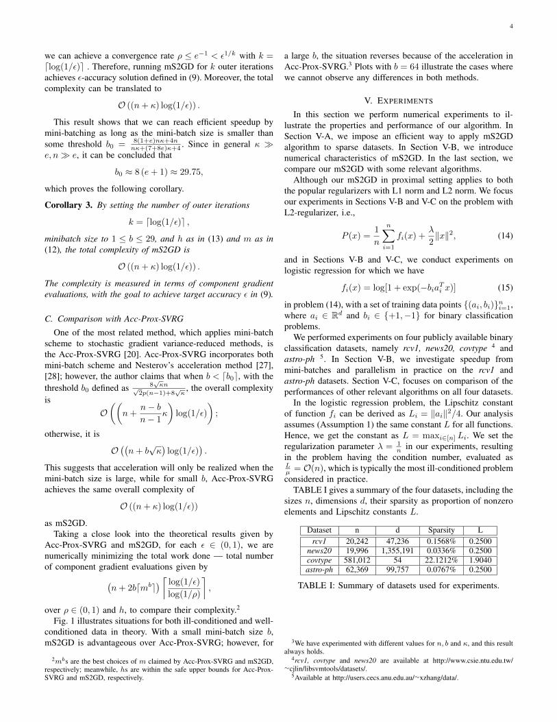
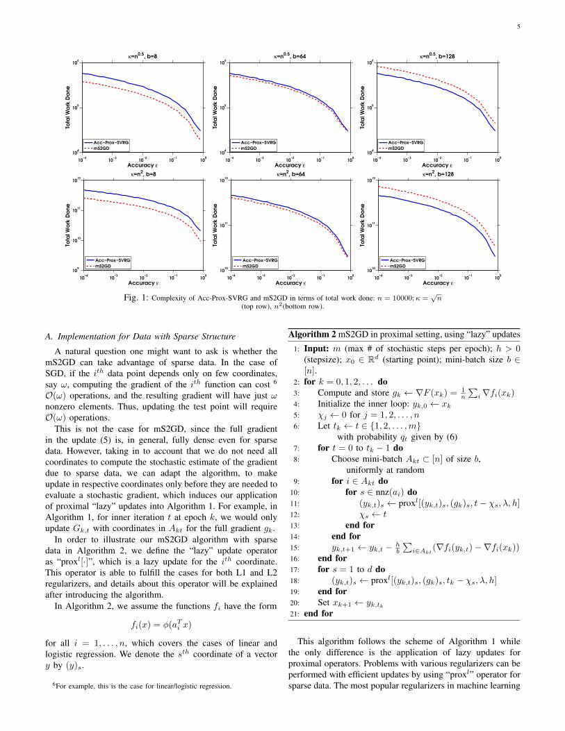
Fig. 1 illustrates situations for both ill-conditioned and well-conditioned data in theory. With a small mini-batch size b,mS2GD is advantageous over Acc-Prox-SVRG; however, for

2mbs are the best choices of m claimed by Acc-Prox-SVRG and mS2GD,respectively; meanwhile, hs are within the safe upper bounds for Acc-Prox-SVRG and mS2GD, respectively.

a large b, the situation reverses because of the acceleration inAcc-Prox-SVRG.3 Plots with b = 64 illustrate the cases wherewe cannot observe any differences in both methods.

V. EXPERIMENTS

In this section we perform numerical experiments to il-lustrate the properties and performance of our algorithm. InSection V-A, we impose an efficient way to apply mS2GDalgorithm to sparse datasets. In Section V-B, we introducenumerical characteristics of mS2GD. In the last section, wecompare our mS2GD with some relevant algorithms.

Although our mS2GD in proximal setting applies to boththe popular regularizers with L1 norm and L2 norm. We focusour experiments in Sections V-B and V-C on the problem withL2-regularizer, i.e.,

P (x) =1

n

n∑i=1

fi(x) +λ

2‖x‖2, (14)

and in Sections V-B and V-C, we conduct experiments onlogistic regression for which we have

fi(x) = log[1 + exp(−biaTi x)] (15)

in problem (14), with a set of training data points {(ai, bi)}ni=1,where ai ∈ Rd and bi ∈ {+1,−1} for binary classificationproblems.

We performed experiments on four publicly available binaryclassification datasets, namely rcv1, news20, covtype 4 andastro-ph 5. In Section V-B, we investigate speedup frommini-batches and parallelism in practice on the rcv1 andastro-ph datasets. Section V-C, focuses on comparison of theperformances of other relevant algorithms on all four datasets.

In the logistic regression problem, the Lipschitz constantof function fi can be derived as Li = ‖ai‖2/4. Our analysisassumes (Assumption 1) the same constant L for all functions.Hence, we get the constant as L = maxi∈[n] Li. We set theregularization parameter λ = 1

n in our experiments, resultingin the problem having the condition number, evaluated asLµ = O(n), which is typically the most ill-conditioned problemconsidered in practice.

TABLE I gives a summary of the four datasets, including thesizes n, dimensions d, their sparsity as proportion of nonzeroelements and Lipschitz constants L.

Dataset n d Sparsity Lrcv1 20,242 47,236 0.1568% 0.2500

news20 19,996 1,355,191 0.0336% 0.2500covtype 581,012 54 22.1212% 1.9040astro-ph 62,369 99,757 0.0767% 0.2500

TABLE I: Summary of datasets used for experiments.

3We have experimented with different values for n, b and κ, and this resultalways holds.

4rcv1, covtype and news20 are available at http://www.csie.ntu.edu.tw/∼cjlin/libsvmtools/datasets/.

5Available at http://users.cecs.anu.edu.au/∼xzhang/data/.

5

10−4

10−3

10−2

10−1

100

104

105

106

κ=n0.5

, b=8

Accuracy ε

Tota

l W

ork

Do

ne

Acc−Prox−SVRG

mS2GD

10−4

10−3

10−2

10−1

100

104

105

106

κ=n0.5

, b=64

Accuracy ε

Tota

l W

ork

Do

ne

Acc−Prox−SVRG

mS2GD

10−4

10−3

10−2

10−1

100

104

105

106

κ=n0.5

, b=128

Accuracy ε

Tota

l W

ork

Do

ne

Acc−Prox−SVRG

mS2GD

10−4

10−3

10−2

10−1

100

109

1010

1011

1012

κ=n2, b=8

Accuracy ε

Tota

l W

ork

Do

ne

Acc−Prox−SVRG

mS2GD

10−4

10−3

10−2

10−1

100

1010

1011

1012

κ=n2, b=64

Accuracy ε

Tota

l W

ork

Do

ne

Acc−Prox−SVRG

mS2GD

10−4

10−3

10−2

10−1

100

1010

1011

1012

κ=n2, b=128

Accuracy ε

Tota

l W

ork

Do

ne

Acc−Prox−SVRG

mS2GD

Fig. 1: Complexity of Acc-Prox-SVRG and mS2GD in terms of total work done: n = 10000;κ =√n

(top row), n2(bottom row).

A. Implementation for Data with Sparse Structure

A natural question one might want to ask is whether themS2GD can take advantage of sparse data. In the case ofSGD, if the ith data point depends only on few coordinates,say ω, computing the gradient of the ith function can cost 6

O(ω) operations, and the resulting gradient will have just ωnonzero elements. Thus, updating the test point will requireO(ω) operations.

This is not the case for mS2GD, since the full gradientin the update (5) is, in general, fully dense even for sparsedata. However, taking in to account that we do not need allcoordinates to compute the stochastic estimate of the gradientdue to sparse data, we can adapt the algorithm, to makeupdate in respective coordinates only before they are needed toevaluate a stochastic gradient, which induces our applicationof proximal “lazy” updates into Algorithm 1. For example, inAlgorithm 1, for inner iteration t at epoch k, we would onlyupdate Gk,t with coordinates in Akt for the full gradient gk.

In order to illustrate our mS2GD algorithm with sparsedata in Algorithm 2, we define the “lazy” update operatoras “proxl[·]”, which is a lazy update for the ith coordinate.This operator is able to fulfill the cases for both L1 and L2regularizers, and details about this operator will be explainedafter introducing the algorithm.

In Algorithm 2, we assume the functions fi have the form

fi(x) = φ(aTi x)

for all i = 1, . . . , n, which covers the cases of linear andlogistic regression. We denote the sth coordinate of a vectory by (y)s.

6For example, this is the case for linear/logistic regression.

Algorithm 2 mS2GD in proximal setting, using “lazy” updates

1: Input: m (max # of stochastic steps per epoch); h > 0(stepsize); x0 ∈ Rd (starting point); mini-batch size b ∈[n].

2: for k = 0, 1, 2, . . . do3: Compute and store gk ← ∇F (xk) = 1

n

∑i∇fi(xk)

4: Initialize the inner loop: yk,0 ← xk5: χj ← 0 for j = 1, 2, . . . , n6: Let tk ← t ∈ {1, 2, . . . ,m}

. with probability qt given by (6)7: for t = 0 to tk − 1 do8: Choose mini-batch Akt ⊂ [n] of size b,

. uniformly at random9: for i ∈ Akt do

10: for s ∈ nnz(ai) do11: (yk,t)s ← proxl[(yk,t)s, (gk)s, t− χs, λ, h]12: χs ← t13: end for14: end for15: yk,t+1 ← yk,t − h

b

∑i∈Akt(∇fi(yk,t)−∇fi(xk))

16: end for17: for s = 1 to d do18: (yk,t)s ← proxl[(yk,t)s, (gk)s, tk − χs, λ, h]19: end for20: Set xk+1 ← yk,tk21: end for

This algorithm follows the scheme of Algorithm 1 whilethe only difference is the application of lazy updates forproximal operators. Problems with various regularizers can beperformed with efficient updates by using “proxl” operator forsparse data. The most popular regularizers in machine learning

6

research are L1 and L2 regularizers. The following lemmasinclude details about proximal lazy updates with L2 and L1regularizers, respectively.

Lemma 1 (Proximal Lazy Updates with L2 Regularizer). Forthe problem (14), which has L2 regularizer in (1) (λ 6= 0) ,our mS2GD algorithm can efficiently perform proximal lazyupdates for sparse data by using the following operator inAlgorithm 2.

proxl[(yk,t)s,(gk)s, τ, λ, h] = βτ (yk,t)s − hβ1−β [1− βτ ] (gk)s,

where s corresponds to the sth coordinate and βdef= 1/(1+λh)

is predefined.

Lemma 2 (Proximal Lazy Updates with L1 Regularizer).Consider problem (1) with L1 regularizer R(x) = ‖x‖1.Our mS2GD algorithm can efficiently update the iterates forsparse data by using the proximal lazy update operator inAlgorithm 2. Define M and m as follows,

M = [λ+ (gk)s]h, m = −[λ− (gk)s]h,

then the forms of the operator are distinct in the followingthree situations, according to the value of (gk)s.

1) If (gk)s ≥ λ, then by letting pdef=⌈(yk)sM

⌉−1, the operator

can be defined as

proxl[(yk,t)s, (gk)s, τ, λ, h]

=

{(yk,t)s − τM, if p ≥ τ,min{(yk,t)s,m}+ (max{p, 0} − τ)m, if p < τ.

2) If −λ < (gk)s < λ, then the operator can be defined as

proxl[(yk,t)s, (gk)s, τ, λ, h]

=

{max{(yk,t)s − τM, 0}, if (yk)s ≥ 0,

min{(yk,t)s − τm, 0}, if (yk)s < 0.

3) If (gk)s ≤ −λ, then by letting qdef=⌈(yk,t)sm

⌉− 1, the

operator can be defined as

proxl[(yk,t)s, (gk)s, τ, λ, h]

=

{(yk,t)s − τm, if q ≥ τ,max{(yk,t)s,M}+ (max{q, 0} − τ)M, if q < τ.

The proofs of Lemmas 1 and 2 are available in AP-PENDIX C.

B. Speedup of mS2GD

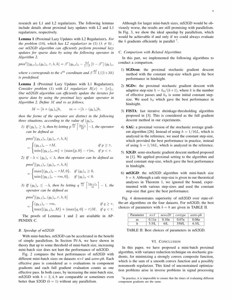
With mini-batches, mS2GD can be accelerated in the benefitof simple parallelism. In Section IV-A, we have shown intheory that up to some threshold of mini-batch size, increasingmini-batch size does not hurt the performance of mS2GD.

Fig. 2 compares the best performances of mS2GD withdifferent mini-batch sizes on datasets rcv1 and astro-ph. Eacheffective pass is considered as n evaluations in componentgradients and each full gradient evaluation counts as oneeffective pass. In both cases, by increasing the mini-batch size,mS2GD with b = 2, 4, 8 are comparable or sometimes evenbetter than S2GD (b = 1) without any parallelism.

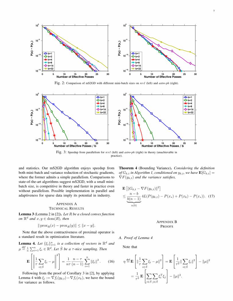
Although for larger mini-batch sizes, mS2GD would be ob-viously worse, the results are still promising with parallelism.In Fig. 3, we show the ideal speedup by parallelism, whichwould be achievable if and only if we could always evaluatethe b gradients efficiently in parallel 7.

C. Comparison with Related Algorithms

In this part, we implemented the following algorithms toconduct a comparison.

1) SGDcon: the proximal stochastic gradient descentmethod with the constant step-size which gave the bestperformance in hindsight.

2) SGD+: the proximal stochastic gradient descent withadaptive step-size h = h0/(k+1), where k is the numberof effective passes and h0 is some initial constant step-size. We used h0 which gave the best performance inhindsight.

3) FISTA: fast iterative shrinkage-thresholding algorithmproposed in [3]. This is considered as the full gradientdescent method in our experiments.

4) SAG: a proximal version of the stochastic average gradi-ent algorithm [26]. Instead of using h = 1/16L, which isanalyzed in the reference, we used the constant step-size,which provided the best performance in practice, insteadof using h = 1/16L, which is analyzed in the reference.

5) S2GD: semi-stochastic gradient descent method proposedin [1]. We applied proximal setting to the algorithm andused constant step-size, which gave the best performancein hindsight.

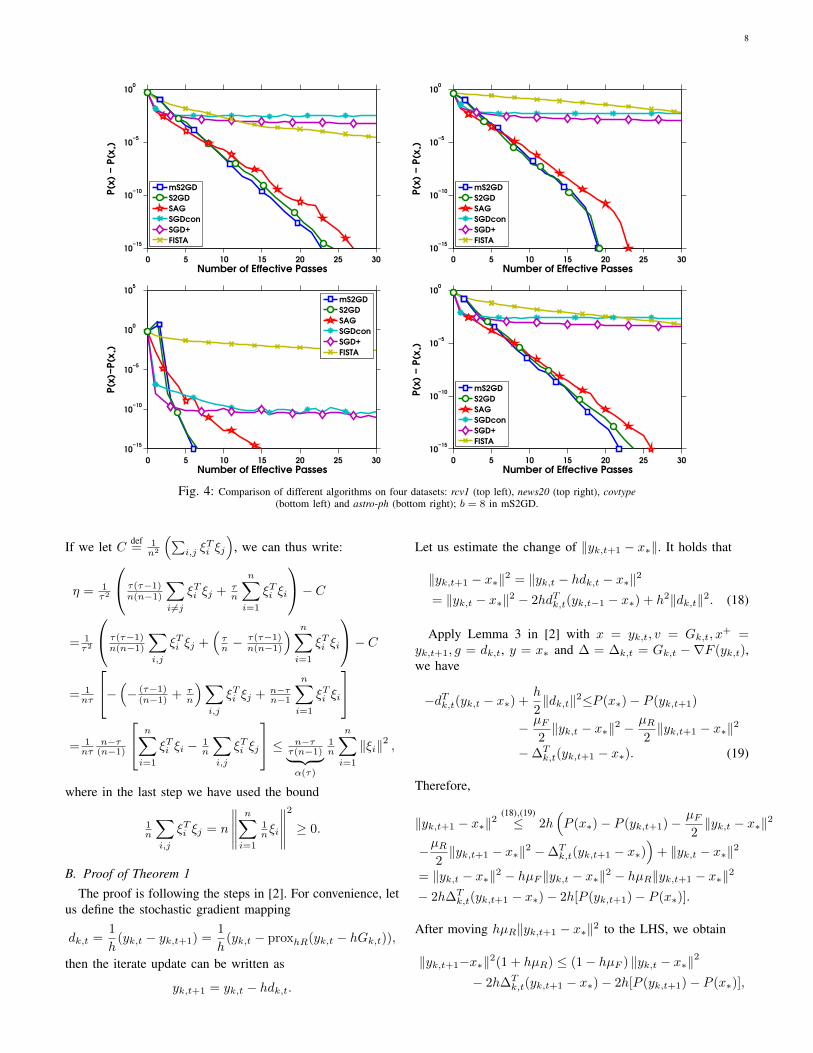
6) mS2GD: the mS2GD algorithm with mini-batch sizeb = 8. Although a safe step-size is given in our theoreticalanalyses in Theorem 1, we ignored the bound, exper-imented with various step-sizes and used the constantstep-size that gave the best performance.

Fig. 4 demonstrates superiority of mS2GD over state-of-the-art algorithms on the four datasets. For mS2GD, the bestchoices of parameters with b = 8 are given in TABLE II.

Parameter rcv1 news20 covtype astro-phm 0.11n 0.10n 0.07n 0.08nh 5.5/L 6/L 350/L 6.5/L

TABLE II: Best choices of parameters in mS2GD.

VI. CONCLUSION

In this paper, we have proposed a mini-batch proximalalgorithm, with variance reduction technique on stochastic gra-dients, for minimizing a strongly convex composite function,which is the sum of a smooth convex function and a possiblynonsmooth regularizer. This kind of unconstrained optimiza-tion problems arise in inverse problems in signal processing

7In practice, it is impossible to ensure that the times of evaluating differentcomponent gradients are the same.

7

0 5 10 15 20 25 30

10−15

10−10

10−5

100

Number of Effective Passes

P(x

) −

P(x

*)

b=1

b=2

b=4

b=8

b=16

b=32

0 5 10 15 20 25 30

10−15

10−10

10−5

100

Number of Effective Passes

P(x

) −

P(x

*)

b=1

b=2

b=4

b=8

b=16

b=32

Fig. 2: Comparison of mS2GD with different mini-batch sizes on rcv1 (left) and astro-ph (right).

0 5 10 15 20 25 30

10−15

10−10

10−5

100

Number of Effective Passes / b

P(x

) −

P(x

*)

b=1

b=2

b=4

b=8

b=16

b=32

0 5 10 15 20 25 30

10−15

10−10

10−5

100

Number of Effective Passes / b

P(x

) −

P(x

*)

b=1

b=2

b=4

b=8

b=16

b=32

Fig. 3: Speedup from parallelism for rcv1 (left) and astro-ph (right) in theory (unachievable inpractice).

and statistics. Our mS2GD algorithm enjoys speedup fromboth mini-batch and variance reduction of stochastic gradients,where the former admits a simple parallelism. Comparisons tostate-of-the-art algorithms suggest mS2GD, with a small mini-batch size, is competitive in theory and faster in practice evenwithout parallelism. Possible implementation in parallel andadaptiveness for sparse data imply its potential in industry.

APPENDIX ATECHNICAL RESULTS

Lemma 3 (Lemma 2 in [2]). Let R be a closed convex functionon Rd and x, y ∈ dom(R), then

‖proxR(x)− proxR(y)‖ ≤ ‖x− y‖.

Note that the above contractiveness of proximal operator isa standard result in optimization literature.

Lemma 4. Let {ξi}ni=1 is a collection of vectors in Rd andµ

def= 1

n

∑ni=1 ξi ∈ Rd. Let S be a τ -nice sampling. Then

E

∥∥∥∥∥∥1

τ

∑i∈S

ξi − µ

∥∥∥∥∥∥2 =

1

nτ

n− τ(n− 1)

n∑i=1

‖ξi‖2 . (16)

Following from the proof of Corollary 3 in [2], by applyingLemma 4 with ξi := ∇fi(yk,t)−∇fi(xk), we have the boundfor variance as follows.

Theorem 4 (Bounding Variance). Considering the definitionof Gk,t in Algorithm 1, conditioned on yk,t, we have E[Gk,t] =∇F (yk,t) and the variance satisfies,

E[‖Gk,t −∇F (yk,t)‖2

]≤ n− bb(n− 1)︸ ︷︷ ︸α(b)

4L(P (yk,t)− P (x∗) + P (xk)− P (x∗)). (17)

APPENDIX BPROOFS

A. Proof of Lemma 4

Note that

ηdef= E

‖1

τ

∑i∈S

ξi − µ‖2 = E

1

τ2‖∑i∈S

ξi‖2− ‖µ‖2

=1

τ2E

∑i∈S

∑j∈S

ξTi ξj

− ‖µ‖2.

8

0 5 10 15 20 25 30

10−15

10−10

10−5

100

Number of Effective Passes

P(x

) −

P(x

*)

mS2GD

S2GD

SAG

SGDcon

SGD+

FISTA

0 5 10 15 20 25 30

10−15

10−10

10−5

100

Number of Effective Passes

P(x

) −

P(x

*)

mS2GD

S2GD

SAG

SGDcon

SGD+

FISTA

0 5 10 15 20 25 30

10−15

10−10

10−5

100

105

Number of Effective Passes

P(x

)−P

(x*)

mS2GD

S2GD

SAG

SGDcon

SGD+

FISTA

0 5 10 15 20 25 30

10−15

10−10

10−5

100

Number of Effective Passes

P(x

) −

P(x

*)

mS2GD

S2GD

SAG

SGDcon

SGD+

FISTA

Fig. 4: Comparison of different algorithms on four datasets: rcv1 (top left), news20 (top right), covtype(bottom left) and astro-ph (bottom right); b = 8 in mS2GD.

If we let C def= 1

n2

(∑i,j ξ

Ti ξj

), we can thus write:

η = 1τ2

τ(τ−1)n(n−1)

∑i6=j

ξTi ξj + τn

n∑i=1

ξTi ξi

− C= 1τ2

τ(τ−1)n(n−1)

∑i,j

ξTi ξj +(τn −

τ(τ−1)n(n−1)

) n∑i=1

ξTi ξi

− C= 1nτ

−(− (τ−1)(n−1) + τ

n

)∑i,j

ξTi ξj + n−τn−1

n∑i=1

ξTi ξi

= 1nτ

n−τ(n−1)

n∑i=1

ξTi ξi − 1n

∑i,j

ξTi ξj

≤ n−ττ(n−1)︸ ︷︷ ︸α(τ)

1n

n∑i=1

‖ξi‖2 ,

where in the last step we have used the bound

1n

∑i,j

ξTi ξj = n

∥∥∥∥∥n∑i=1

1nξi

∥∥∥∥∥2

≥ 0.

B. Proof of Theorem 1

The proof is following the steps in [2]. For convenience, letus define the stochastic gradient mapping

dk,t =1

h(yk,t − yk,t+1) =

1

h(yk,t − proxhR(yk,t − hGk,t)),

then the iterate update can be written as

yk,t+1 = yk,t − hdk,t.

Let us estimate the change of ‖yk,t+1 − x∗‖. It holds that

‖yk,t+1 − x∗‖2 = ‖yk,t − hdk,t − x∗‖2

= ‖yk,t − x∗‖2 − 2hdTk,t(yk,t−1 − x∗) + h2‖dk,t‖2. (18)

Apply Lemma 3 in [2] with x = yk,t, v = Gk,t, x+ =

yk,t+1, g = dk,t, y = x∗ and ∆ = ∆k,t = Gk,t − ∇F (yk,t),we have

−dTk,t(yk,t − x∗) +h

2‖dk,t‖2≤P (x∗)− P (yk,t+1)

− µF2‖yk,t − x∗‖2 −

µR2‖yk,t+1 − x∗‖2

−∆Tk,t(yk,t+1 − x∗). (19)

Therefore,

‖yk,t+1 − x∗‖2(18),(19)≤ 2h

(P (x∗)− P (yk,t+1)− µF

2‖yk,t − x∗‖2

−µR2‖yk,t+1 − x∗‖2 −∆T

k,t(yk,t+1 − x∗))

+ ‖yk,t − x∗‖2

= ‖yk,t − x∗‖2 − hµF ‖yk,t − x∗‖2 − hµR‖yk,t+1 − x∗‖2

− 2h∆Tk,t(yk,t+1 − x∗)− 2h[P (yk,t+1)− P (x∗)].

After moving hµR‖yk,t+1 − x∗‖2 to the LHS, we obtain

‖yk,t+1−x∗‖2(1 + hµR) ≤ (1− hµF ) ‖yk,t − x∗‖2

− 2h∆Tk,t(yk,t+1 − x∗)− 2h[P (yk,t+1)− P (x∗)],

9

and dividing both sides by (1 + hµF ) gives us

‖yk,t+1 − x∗‖2 ≤ α ‖yk,t − x∗‖2

+2h

1 + hµR

(−∆T

k,t(yk,t+1 − x∗)− [P (yk,t+1)− P (x∗)]).

(20)

In order to bound −∆Tk,t(yk,t+1 − x∗), let us define the

proximal full gradient update as8

yk,t+1 = proxhR(yk,t − h∇F (yk,t)),

with which, by using Cauchy-Schwartz inequality andLemma 3, we can conclude that

−∆Tk,t(yk,t+1 − x∗)

= −∆Tk,t(yk,t+1 − yk,t+1)−∆T

k,t(yk,t+1 − x∗)= −∆T

k,t(yk,t+1 − x∗)−∆Tk,t[proxhR(yk,t − hGk,t)

− proxhR(yk,t−1 − h∇F (yk,t−1))]

≤ ‖∆k,t‖‖(yk,t − hGk,t)− (yk,t − h∇F (yk,t))‖−∆T

k,t(yk,t+1 − x∗),= h‖∆k,t‖2 −∆T

k,t(yk,t+1 − x∗). (21)

Letting δ def= 1−hµF

1+hµR, we thus get

‖yk,t+1 − x∗‖2(21),(20)≤ δ ‖yk,t − x∗‖2

+ 2h1+hµR

(h‖∆k,t‖2 −∆T

k,t(yk,t+1 − x∗)−[P (yk,t+1)− P (x∗)]) .

By taking expectation, conditioned on yk,t9 we obtain

E[‖yk,t+1 − x∗‖2](21),(20)≤ δ ‖yk,t − x∗‖2

+ 2h1+hµR

(hE[‖∆k,t‖2]−E[P (yk,t+1)− P (x∗)]

), (22)

where we have used that E[∆k,t] = E[Gk,t]−∇F (yk,t) = 0and hence E[−∆T

k,t(yk,t+1 − x∗)] = 010. Now, if we put (17)into (22) and decrease index t by 1, we obtain

E[‖yk,t − x∗‖2](21),(20)≤ δ ‖yk,t−1 − x∗‖2

+ 2h1+hµR

{4Lhα(b)[P (yk,t−1)− P (x∗)

+ P (xk)− P (x∗)]−E[P (yk,t)− P (x∗)]}, (23)

where α(b) = n−bb(n−1) .

Now recall that we assume that we have lower-bounds νF ≥0 and νR ≥ 0 on the true strong convexity parameter µF andµR available. Letting

δ′def= 1−hνF

1+hνR,

we obtain from (23) that

E[‖yk,t − x∗‖2](23)≤ δ′ ‖yk,t−1 − x∗‖2

+ 2h1+hνR

{4Lhα(b)(P (yk,t−1)− P (x∗)

+ P (xk)− P (x∗))−E[P (yk,t)− P (x∗)]},

8Note that this quantity is never computed during the algorithm. We canuse it in the analysis nevertheless.

9For simplicity, we omit the E[· | yk,t] notation in further analysis10yk,t+1 is constant, conditioned on yk,t

which is equivalent to

E[‖yk,t − x∗‖2] + 2h1+hνR

(E[P (yk,t)− P (x∗)])

≤ δ′ ‖yk,t−1 − x∗‖2

+ 8h2Lα(b)1+hνR

(P (yk,t−1)− P (x∗) + P (xk)− P (x∗)).

(24)

Now, by the definition of xk we have that

E[P (xk+1)] = 1γ

m∑t=1

(δ′)m−t

E[P (yk,t)], (25)

where γ =∑mt=1 (δ′)

m−t. By summing (24), multiplied by(δ′)

m−t for t = 1, . . . ,m, we obtain on the left hand side

LHS =

m∑t=1

(δ′)m−t

E[‖yk,t − x∗‖2]

+ 2h1+hνR

m∑t=1

(δ′)m−t

E[P (yk,t)− P (x∗)] (26)

and for the right hands side we have:

RHS =

m∑t=1

(δ′)m−t+1

E ‖yk,t−1 − x∗‖2

+ 8h2Lα(b)1+hνR

m∑t=1

(δ′)m−t

E[P (yk,t−1)

−P (x∗) + P (xk)− P (x∗)]

=

m−1∑t=0

(δ′)m−t

E ‖yk,t − x∗‖2

+ 8h2Lα(b)1+hνR

1δ′ ·(m−1∑t=0

(δ′)m−t

E[P (yk,t)− P (x∗)]

)+ 8h2Lα(b)

1+hνRE[P (xk)− P (x∗)]γ.

Therefore,

RHS ≤m−1∑t=0

(δ′)m−t

E ‖yk,t − x∗‖2

+ 8h2Lα(b)1+hνR

1+hνR1−hνF ·

(m∑t=0

(δ′)m−t

E[P (yk,t)− P (x∗)]

)+ 8h2Lα(b)

1+hνRE[P (xk)− P (x∗)]γ. (27)

Combining (26) and (27) and using the fact that LHS ≤RHS, we have

E[‖yk,m − x∗‖2] + 2h1+hνR

m∑t=1

(δ′)m−t

E[P (yk,t)− P (x∗)]

≤ (δ′)mE ‖yk,0 − x∗‖2

+ 8h2Lα(b)1+hνR

E[P (xk)− P (x∗)]γ + 8h2Lα(b)1+hνR

1+hνR1−hνF

·(

m∑t=1

(δ′)m−t

E[P (yk,t)− P (x∗)]

)+ 8h2Lα(b)

1+hνR1+hνR1−hνF

((δ′)

mE[P (yk,0)− P (x∗)]

).

10

Now, using (25), we obtain

E[‖yk,m − x∗‖2] + 2h1+hνR

γ(E[P (xk+1)]− P (x∗))

≤ (δ′)mE ‖yk,0 − x∗‖2 + 8h2Lα(b)

1+hνRγE[P (xk)− P (x∗)]

+ 8h2Lα(b)1+hνR

1δ′ γ (E[P (xk+1)]− P (x∗))

+ 8h2Lα(b)1+hνR

1δ (δ′)

mE[P (yk,0)− P (x∗)]. (28)

Strong convexity (3) and optimality of x∗ imply that 0 ∈∂P (x∗), and hence for all x ∈ Rd we have

‖x− x∗‖2 ≤ 2µ [P (x)− P (x∗)]. (29)

Since E ‖yk,m − x∗‖2 ≥ 0 and yk,0 = xk, by combining (29)and (28) we get

2γh{

11+hνR

− 4hLα(b)1−hνF

}(E[P (xk+1)]− P (x∗))

≤ (P (xk)− P (x∗)){

(δ′)m 2µ + 8h2Lα(b)

1+hνR

(γ + (δ′)

m−1)}

.

This is equivalent to

E[P (xk+1)− P (x∗)] ≤ ρ[P (xk)− P (x∗)],

when 11+hνR

− 4hLα(b)1−hνF > 0 (which is equivalent to

1−hνF1+hνR

14Lα(b) ≥ h ), and when ρ is defined as

ρ =

(1−hνF1+hνR

)m1µ + 4h2Lα(b)

1+hνR

(γ +

(1−hνF1+hνR

)m−1)γh{

11+hνR

− 4hLα(b)1−hνF

} .

The above statement, together with assumptions ofLemma 3 in [2], implies

0 < h < min{

1−hνF1+hνR

14Lα(b) ,

1L

}.

Applying the above linear convergence relation recursivelywith chained expectations, we have

E[P (xk)− P (x∗)] ≤ ρk[P (x0)− P (x∗)].

C. Proof of Theorem 2

Clearly, if we choose some value of h then the value of mwill be determined from (8) (i.e. we need to choose m suchthat we will get desired rate). Therefore, m as a function ofh obtained from (8) is

m(h) =1 + 4α(b)h2Lµ

hµ(ρ− 4α(b)hL(ρ+ 1)). (30)

Now, we can observe that the nominator is always positiveand the denominator is positive only if

ρ > 4α(b)hL(ρ+ 1)⇒ 1

4α(b)L· ρ

ρ+ 1︸ ︷︷ ︸∈[0, 12 ]

> h.

Note that this condition is stronger than the one in assumptionof Theorem 1. It is easy to verify that

limh↘0

m(h) = +∞, limh↗ 1

4α(b)L· ρρ+1

m(h) = +∞.

Also note that m(h) is differentiable (and continuous) at anyh ∈ (0, 1

4α(b)L ·ρρ+1 ) =: Ih. Let us look at the m′(h). We

have

m′(h) =−ρ+ 4α(b)hL(2 + (2 + hµ)ρ)

h2µ(ρ− 4α(b)hL(1 + ρ))2.

Observe that m′(h) is defined and continuous for any h ∈ Ih.Therefore there have to be some stationary points (and in casethat there is just on Ih) it will be the global minimum on Ih.The FOC gave us that

hb =−2α(b)L(1 + ρ) +

√α(b)L(µρ2 + 4α(b)L(1 + ρ)2)

2α(b)Lµρ

=

√1

4α(b)Lµ+

(1 + ρ)2

µ2ρ2− 1 + ρ

µρ. (31)

If this hb ∈ Ih and also hb ≤ 1L then this is the optimal choice

and plugging (31) into (30) gives us (10).a) Claim #1: It always holds that hb ∈ Ih. We just need

to verify that√1

4α(b)Lµ+

(1 + ρ)2

µ2ρ2− 1 + ρ

µρ<

1

4α(b)L· ρ

ρ+ 1,

which is equivalent to

µρ2 + 4α(b)L(1 + ρ)2

> 2(1 + ρ)√α(b)L(µρ2 + 4α(b)L(1 + ρ)2).

Because both sides are positive, we can square them to obtainan equivalent condition(

µρ2 + 4α(b)L(1 + ρ)2)2

> 4(1 + ρ)2α(b)L(µρ2 + 4α(b)L(1 + ρ)2),

which is equivalent with

µρ2(µρ2 + 4α(b)L(1 + ρ)2) > 0.

b) Claim #2: If hb > 1L then hb∗ = 1

L . I believe that thisis trivial.

Only one thing which needs to be verified is that thedenominator of (11) is positive (or equivalently we want toshow that ρ > 4α(b)(1 + ρ). To see that we just need torealize that in that case we have

1

L≤ hb ≤ 1

4α(b)L· ρ

ρ+ 1

which implies that

1 ≤ 1

4α(b)· ρ

ρ+ 1⇒ 4α(b)(1 + ρ) < ρ.

APPENDIX CPROXIMAL LAZY UPDATES FOR L1 AND L2 REGULARIZERS

A. Proof of Lemma 1By applying the updates with proximal operator (4) and L2

regularizer, from Algorithm 1 we have

yk+1,t = proxhR(yk,t − hGk,t)

= arg minx∈Rd

{12 ‖x− (yk,t − hGk,t)‖2 +

λh

2‖x‖2

}=

1

1 + λh(yk,t − hGk,t) = β(yk,t − hGk,t),

11

where β = 1/(1 + λh) and

Gk,t = gk +1

b

∑i∈Akt

(∇fi(yk,t)−∇fi(xk)).

In lazy updates, for the sth coordinate, we have (Gk,t)s =(gk)s, which gives the lazy update for 1 iteration as

(yk+1,t)s = β[(yk,t)s − h(gk)s],

which by being applied recursively, gives lazy updates for τiterations for the sth coordinate as

(yk+τ,t)s = βτ (yk,t)s − h

τ∑j=1

βj

(gk)s

= βτ (yk,t)s −hβ

1− β[1− βτ ] (gk)s

def= proxl[(yk,t)s, (gk)s, τ, λ, h],

when λ 6= 0.

B. Proof of Lemma 2

In (1), by letting R(x) = λ‖x‖1, which is the L1-regularizer, we have the following update from Algorithm 1,

yk+1,t = proxhR(yk,t − hGk,t), (32)

and the proximal operator can be calculated as

proxhR(z) = arg minx

1

2‖x− z‖2 + λh‖x‖1,

where each coordinates are separable, i.e., the sth coordinatefor (32) can be updated as

(yk+1,t)s = arg minx∈R

1

2(x− zs)2 + λh|x|

=

zs − λh, if zs > λh,

0, if − λh ≤ zs ≤ λh,zs + λh, if zs < −λh,

where zs = (yk,t)s − h(Gk,t)s and

Gk,t = gk +1

b

∑i∈Akt

(∇fi(yk,t)−∇fi(xk)).

The lazy update does not include the mini-batch part, whichmeans the lazy update proceeds with (Gk,t)s = (gk)s for eachcoordinate s, therefore,

(yk+1,t)s =(yk,t)s − [λ+ (gk)s]h, if (yk,t)s > [λ+ (gk)s]h,

0, if − [λ− (gk)s]h ≤ (yk,t)s ≤ [λ+ (gk)s]h,

(yk,t)s + [λ− (gk)s]h, if (yk,t)s < −[λ− (gk)s]h,

and notice that (λ + (gk)s)h − [−(λ − (gk)s)] = 2λh > 0.Depending on the value of (gk)s, there would be threesituations for τ lazy updates listed as follows.

(1) When −λ < (gk)s < λ, then λ + (gk)s > 0,−[λ −(gk)s] < 0, thus we have that

(yk+τ,t)s ={max{(yk,t)i − τ [λ+ (gk)s]h, 0}, if (yk,t)s ≥ 0,

min{(yk,t)s + τ [λ− (gk)s]h, 0}, if (yk,t)s < 0.

(2) When (gk)s ≥ λ, then −[λ − (gk)s] ≥ 0, λ + (gk)s ≥2λ > 0, thus by letting p =

⌈(yk)s

[λ+(gk)s]h

⌉− 1, we have

that:if (yk,t)s > [λ+ (gk)s]h, then

(yk+τ,t)s =

{(yk,t)s − τ [λ+ (gk)s]h, if τ ≤ p,(τ − p− 1)[λ− (gk)s]h, if τ > p;

if (yk,t)s < −[λ− (gk)s]h, then

(yk+τ,t)s = (yk,t)s + τ [λ− (gk)s]h;

if −[λ− (gk)s] ≤ (yk,t)s ≤ [λ+ (gk)s], then

(yk+τ,t)s = (τ − 1)[λ− (gk)s]h.

(3) When (gk)s ≤ −λ, then λ+ (gk)s ≤ 0, −[λ− (gk)s] ≤−2λ < 0, thus by letting q =

⌈(yk,t)s

−[λ−(gk)s]h

⌉−1, we have

that:if (yk,t)s ≥ [λ+ (gk)s], then

(yk+τ,t)s = (yk,t)s − τ [λ+ (gk)s]h;

if (yk,t)s < −[λ− (gk)s], then

(yk+τ,t)s =

{(yk,t)s + τ [λ− (gk)s]h, if τ ≤ q,−(τ − q − 1)[λ+ (gk)s]h, if τ > q;

if −[λ− (gk)s] ≤ (yk,t)s ≤ [λ+ (gk)s], then

(yk+τ,t)s = −(τ − 1)[λ+ (gk)s]h.

For Case (2), when (yk,t)s ≤ [λ+ (gk)s], we can concludethat

(yk+τ,t)s = min{(yk,t)s,−[λ− (gk)s]h}+ τ [λ− (gk)s]h.

Moreover, the following equivalences hold under the condition(gk)s ≥ λ,

(yk,t)s > [λ+ (gk)s]h ⇔(yk,t)s

[λ+ (gk)s]h> 1 ⇔ p ≥ 1,

(yk,t)s ≤ [λ+ (gk)s]h ⇔(yk,t)s

[λ+ (gk)s]h≤ 1 ⇔ p ≤ 0,

which simplifies the situation to

(yk+τ,t)s

=

(yk,t)s − τ [λ+ (gk)s]h, if p ≥ τ(τ − p− 1)[λ− (gk)s]h, if 1 ≤ p < τ

min{(yk,t)s,−[λ− (gk)s]h}+τ [λ− (gk)s]h, if p ≤ 0

=

(yk,t)s − τ [λ+ (gk)s]h, if p ≥ τ,min{(yk,t)s,−[λ− (gk)s]h}

+(τ −max{p, 0})[λ− (gk)s]h, if p < τ.

12

For Case (3), when (yk,t)s ≥ −[λ − (gk)s]h, we canconclude that

(yk+τ,t)s = max{(yk,t)s, λ+ (gk)s} − τ [λ+ (gk)s]h,

and in addition, the following equivalences hold when (gk)s ≤−λ,

(yk,t)s < −[λ− (gk)s]h ⇔(yk,t)s

−[λ− (gk)s]h> 1 ⇔ q ≥ 1,

(yk,t)s ≥ −[λ− (gk)s]h ⇔(yk,t)s

−[λ− (gk)s]h≤ 1 ⇔ q ≤ 0,

which can summarize the situation as

(yk+τ,t)s

=

(yk,t)s + τ [λ− (gk)s]h, if q ≥ τ−(τ − q − 1)[λ+ (gk)s]h, if 1 ≤ q < τ

max{(yk,t)s, [λ+ (gk)s]h}−τ [λ+ (gk)s]h, if q ≤ 0

=

(yk,t)s + τ [λ− (gk)s]h, if q ≥ τ,max{(yk,t)s, [λ+ (gk)s]h}

+(max{q, 0} − τ)[λ+ (gk)s]h, if q < τ.

The proof can be completed by letting M = [λ + (gk)s]hand m = −[λ− (gk)s]h.

REFERENCES

[1] J. Konecny and P. Richtarik, “Semi-stochastic gradient descent meth-ods,” arXiv:1312.1666, 2013.

[2] L. Xiao and T. Zhang, “A proximal stochastic gradient method withprogressive variance reduction,” SIAM Journal on Optimization, vol. 24,no. 4, pp. 2057–2075, 2014.

[3] A. Beck and M. Teboulle, “A fast iterative shrinkage-thresholdingalgorithm for linear inverse problems,” SIAM J. Imaging Sciences, vol. 2,no. 1, pp. 183–202, 2009.

[4] Y. Nesterov, “Efficiency of coordinate descent methods on huge-scaleoptimization problems,” SIAM J. Optimization, vol. 22, pp. 341–362,2012.

[5] P. Richtarik and M. Takac, “Iteration complexity of randomized block-coordinate descent methods for minimizing a composite function,”Mathematical Programming, vol. 144, no. 1-2, pp. 1–38, 2014.

[6] P. Richtarik and M. Takac, “Parallel coordinate descent methods for bigdata optimization,” arXiv:1212.0873, 2012.

[7] I. Necoara and A. Patrascu, “A random coordinate descent algorithmfor optimization problems with composite objective function and linearcoupled constraints,” Comp. Optimization and Applications, vol. 57,no. 2, pp. 307–337, 2014.

[8] O. Fercoq and P. Richtarik, “Accelerated, parallel and proximal coordi-nate descent,” arXiv:1312.5799, 2013.

[9] S. Shalev-Shwartz and T. Zhang, “Stochastic dual coordinate ascentmethods for regularized loss,” JMLR, vol. 14, no. 1, pp. 567–599, 2013.

[10] J. Marecek, P. Richtarik, and M. Takac, “Distributed block coordinatedescent for minimizing partially separable functions,” arXiv:1406.0238,2014.

[11] I. Necoara and D. Clipici, “Distributed coordinate descent methods forcomposite minimization,” arXiv:1312.5302, 2013.

[12] P. Richtarik and M. Takac, “Distributed coordinate descent method forlearning with big data,” arXiv:1310.2059, 2013.

[13] O. Fercoq, Z. Qu, P. Richtarik, and M. Takac, “Fast distributed coor-dinate descent for non-strongly convex losses,” in IEEE Workshop onMachine Learning for Signal Processing, 2014.

[14] T. Zhang, “Solving large scale linear prediction using stochastic gradientdescent algorithms,” in ICML, 2004.

[15] A. Nemirovski, A. Juditsky, G. Lan, and A. Shapiro, “Robust stochasticapproximation approach to stochastic programming,” SIAM J. Optimiza-tion, vol. 19, no. 4, pp. 1574–1609, 2009.

[16] C. Ma, V. Smith, M. Jaggi, M. I. Jordan, P. Richtarik, and M. Takac,“Adding vs. averaging in distributed primal-dual optimization,” arXivpreprint arXiv:1502.03508, 2015.

[17] M. Jaggi, V. Smith, M. Takac, J. Terhorst, T. Hofmann, and M. I.Jordan, “Communication-efficient distributed dual coordinate ascent,”NIPS, 2014.

[18] M. Takac, A. S. Bijral, P. Richtarik, and N. Srebro, “Mini-batch primaland dual methods for SVMs,” ICML, 2013.

[19] R. Johnson and T. Zhang, “Accelerating stochastic gradient descent usingpredictive variance reduction,” NIPS, pp. 315–323, 2013.

[20] A. Nitanda, “Stochastic proximal gradient descent with accelerationtechniques,” NIPS, 2014.

[21] S. Shalev-Shwartz, Y. Singer, N. Srebro, and A. Cotter, “Pegasos: Primalestimated sub-gradient solver for svm,” Mathematical Programming:Series A and B- Special Issue on Optimization and Machine Learning,pp. 3–30, 2011.

[22] O. Dekel, R. Gilad-Bachrach, O. Shamir, and L. Xiao, “Optimal dis-tributed online prediction using mini-batches,” JMLR, vol. 13, no. 1, pp.165–202, 2012.

[23] A. Cotter, O. Shamir, N. Srebro, and K. Sridharan, “Better mini-batchalgorithms via accelerated gradient methods,” in NIPS, 2011, pp. 1647–1655.

[24] P. Zhao and T. Zhang, “Accelerating minibatch stochastic gradientdescent using stratified sampling,” arXiv:1405.3080, 2014.

[25] S. Shalev-Shwartz and T. Zhang, “Accelerated mini-batch stochastic dualcoordinate ascent,” in NIPS, 2013, pp. 378–385.

[26] N. Le Roux, M. Schmidt, and F. Bach, “A stochastic gradient methodwith an exponential convergence rate for finite training sets,” NIPS,2012.

[27] Y. Nesterov, Introductory Lectures on Convex Optimization: A BasicCourse. Kluwer, Boston, 2004.

[28] ——, “Gradient methods for minimizing composite objective function,”CORE Discussion Papers, 2007.