Systems and Analytical Techniques Towards Practical Energy ...

Systems and Analytical Techniques Towards

Practical Energy Breakdown for Homes

by

Nipun Batra

Submitted to the Department of Computer Sciencein partial fulfillment of the requirements for the degree of

Doctor of Philosophy

at the

INDRAPASTHA INSTITUTE OF INFORMATION TECHNOLOGY

March 2017

©IIIT Delhi, 2016. All rights reserved.

Author . . . . . . . . . . . . . . . . . . . . . . . . . . . . . . . . . . . . . . . . . . . . . . . . . . . . . . . . . . . . . .Department of Computer Science

Mar 7, 2017

Certified by. . . . . . . . . . . . . . . . . . . . . . . . . . . . . . . . . . . . . . . . . . . . . . . . . . . . . . . . . .Amarjeet Singh

Assistant ProfessorThesis Supervisor

Certified by. . . . . . . . . . . . . . . . . . . . . . . . . . . . . . . . . . . . . . . . . . . . . . . . . . . . . . . . . .Kamin WhitehouseAssociate Professor

Thesis Supervisor

Accepted by . . . . . . . . . . . . . . . . . . . . . . . . . . . . . . . . . . . . . . . . . . . . . . . . . . . . . . . . .-

IIIT Delhi

2

Systems and Analytical Techniques Towards Practical

Energy Breakdown for Homes

by

Nipun Batra

Submitted to the Department of Computer Scienceon Mar 7, 2017, in partial fulfillment of the

requirements for the degree ofDoctor of Philosophy

Abstract

Buildings contribute significantly to overall energy consumption across the world.Studies suggest that providing occupants with an energy breakdown: per-applianceenergy consumption, can help them save up to 15% energy. However, there arecurrently no practical solutions to provide an energy breakdown. There are threecore problems impeding the practicality of energy breakdown: 1) comparability - it isvirtually impossible to compare two energy breakdown techniques, 2) actionability -current research focuses mostly on giving an energy breakdown, without consideringinsights that can help users save energy, and 3) scalability - current research requireshardware in each home, and thus can not be scaled across all homes. In this thesis, weaddress these three core problems towards making energy breakdown more practical.First, we present open source tools and data sets that make it easier to compareenergy breakdown methods. Second, we present techniques that create actionableenergy saving insights from appliance energy traces. The generated insights such asmodifying thermostat temperature setpoint can save up to 10% energy. Third, wepropose new methods that can provide an energy breakdown, without installing anysensor in the home. Our methods are not only more scalable, they are also up to37% more accurate compared to the state-of-the-art energy breakdown techniques.To summarise, our thesis attempts to make energy breakdown more practical, bymaking it comparable, actionable, and scalable.

Thesis Supervisor: Amarjeet SinghTitle: Assistant Professor

Thesis Supervisor: Kamin WhitehouseTitle: Associate Professor

3

4

Dedication

This thesis is dedicated to my parents and teachers who always wanted me to be

virtuous.

5

Acknowledgments

“The journey of a thousand miles begins with a single step”, so says the ancient

Chinese proverb. While my PhD has spanned only the last 5 years of my life, a good

amount of steps had been taken a long while before my PhD started. In this writeup,

I’d like to acknowledge people who’ve shaped me as a person and without whose

intervention, I could not have been what I am. Of course, I realise my limitations

and my ungratefulness. Thus, I may not be able to thank many people.

I remember as a grade two kid, my class teacher Ms. Marina praising me in front

of the whole class that I’d done really well in exams. That little act of appreciation is

so very firmly impressed in my mind even now. Maybe, if she had not been generous

in her appreciation, I may not have taken my studies the way I did. I also remember

becoming so happy with her appreciation and getting casual that I didn’t study at all

for the final exam. I fared poorly in that particular exam. I heard that my percentage

dropped from 95 to 89. Sure, I really messed the exam. It was a lesson that has stayed

with me all through the years- not to get overconfident! This particular lesson helped

me to form better habits that would eventually help me in my PhD.

I remember changing my school in grade fourth. If it were not for the motherly

care that my then class teacher Mrs. Abnash Kaur gave, I may never have taken my

studies seriously. In grade fifth, my class teacher Mr. Andrew Hoffland impressed

upon us the need to be all round good, rather than just being good in academics. He

wanted us all to read more. That little push in those pre 2000 days went a long way.

A lot of my skills that I would use in my PhD were getting honed.

By this time, I started to realise that my favourite subjects were the ones where

I had my favourite teachers. My mathematics teacher, Mr. KP Joy holds a special

place for me. If not for him, I may have never taken an active interest in mathematics.

I may thus never have been able to do my computer science PhD. I studied not just

for myself, but for Mr. Joy would be happy to see me ace an 100/100. I particularly

remember him asking for my answer sheet when he wanted to discuss the exam

answers. Needless to say, I had a 100/100 on that exam. That particular incident

6

greatly encouraged me! A lot of other teachers, Mrs. Anita Bisht, Mrs. Shobha

Sharma, Mrs. Meenu Sharma, Mrs. P. Singh, encouraged me constantly and thus

honed me to becoming a better person. They showed faith in me, when I had little

faith on myself.

My computer science teachers deserve a very special mention. I was once dis-

cussing with Mrs. Lata Nandkumar about changing to a higher ranked school. She

remarked that it is the students who make the school and not vice versa. This par-

ticular statement has stuck with me through all these years. It would later help me

to focus on what I can do, rather than constantly complain about what I don’t. This

particular incident also helped me to choose IIIT-Delhi to do my PhD. Mr. Geo

Matthew taught us C++ programming. While, I used to miss classes due to engi-

neering entrance preparation, his lessons helped me get stronger at programming.

The programming base that was set by Mrs. Sojan in grade sixth through eight just

got stronger. It convinced me all the more that computer engineering is the field for

me! Mr. Avadesh and Mr. Manish Sharma helped maintain and develop my interest

in the sciences. My chess coach was always very inspiring. He once told me that I

was almost as good as the national youth champion in those early 2000s. I once asked

my grade twelfth mathematics teacher about my chances in the engineering exams.

She told me like another school senior of ours who topped the engineering exams, I

had the ingredients. Looking back, I realise how all these small encouragement have

helped me.

My school time was a great learning experience. Many deep friendships, without

which I may not have developed the character or the skills that greatly helped me

in my PhD. I remember that I didn’t have a personal computer till class ninth. My

school buddy, Raunaq Suri and his parents kindly allowed me to work at their home.

I didn’t even know what Windows was and was greatly helped by Raunaq. The

powerpoint that I learnt in those days, went a great deal in me learning the art of

selling my work. I particularly feel very thankful to Raunaq’s parents who treated

me like their own son.

I was mostly a shy and studious kid. It was only my good friend Shashank Popli’s

7

intervention that helped me grow. He constantly encouraged me to participate in de-

bates, quizzes, symposiums. Our team participated in many inter-school competitions

(we got free sandwiches there!). The confidence gained there went a long way!

My good friend Ritwik Manan formed with me what was a very intense Federer-

Nadal battle. He was one of the smartest guys I have ever seen. Our “friendly”

battles for the top academic position, helped me to become much better. Many of

my other school friends- Shevaal, Shekhar, Arjun, Sharad formed great friendships

that I savour!

Moving on to college was a difficult phase. Some of my new friends Dheeraj, Mohit,

Mayank helped me significantly. I had started to lose faith in the system and interest

in computer science. My friends Sidharth and NIkhil greatly helped me regain that

interest. At the end of the first year, I was inducted into the university Unmanned

Aerial Vehicle (UAV) team. I learnt a lot as a part of the UAV team. My stint there

also helped me a great deal in shaping my interests in research. I understood that

my liking lied in systems and applications. The international exposure that we got

while working on the UAV helped develop a lot of confidence. I also gained a lot

of skills that played a key role in my PhD. Particularly, I learnt from Suraj Joseph-

“if it ain’t broke, don’t fix it. From Rohit Arora I learnt how sincere determination

can help one learn a completely new field (computer vision) in his case. Sahil and

Raghvendra taught me how to be patient while working with hardware. I played with

a lot of hardware in my PhD and I was already prepared in my stint with the UAV

team. Rochak Chadha was the team captain. I learnt from him how much ownership

is needed to successfully complete research projects. I particularly value this lesson

a lot. Abhay and Arjit taught me how rigour, deep interest can help overcome any

shortcomings in coursework.

Rochak Talwar always believed in me and his encouragement helped me a great

deal.

My short stints at Goldman Sachs and RBS were helpful in choosing research.

Working in these banks showed me that I valued intellectual independence and thus

research would be the right move. Encouraged by my friends, Anirvana, Sidharth, I

8

chose to pursue my interest in research and I chose to join IIIT Delhi.

My BTech project mentor, Dr. Divyashikha deserves a very special mention for

being my first formal research mentor. Her honest attempts at setting up laboratories

and improving the standard of education, and her encouragements have helped me a

lot.

The past five years at IIIT Delhi have been filled with a lot of learning and a lot

of experiences that will always stay with me. I feel very grateful towards my advisor,

Dr. Amarjeet Singh. I realise that I am a very pushy researcher and thus can be

very hard to handle for an advisor. The role of an advisor is very strange. They

pick you up when you know nothing about research. They spend blood and sweat in

training you and when you are well-trained, you are ready to leave. Like teaching,

advising is a tough job! Dr. Amarjeet Singh very nicely balanced the line between

being very hands-on versus being very hands-off. In the initial years, he was hands-on

and that allowed me to get bootstrapped into research. Wherever needed, he allowed

me my independence. He is probably one of the most energetic and passionate person

I have ever seen. I remember how hopelessly poor I was in research when I came to

him. I was an engineer when I came to him, I leave as a researcher. The difference

between the two is very wide! Dr. Amarjeet pushed me a lot. When he started to get

more hands-off, I started feeling odd and thought why he’s doing so. Looking back, I

realise how perfectly he timed getting more hands-off. I might have published more

papers with him being hands-on, but, I may have never learnt how to do independent

research. Dr. Amarjeet also always showed a lot of faith in me. Having advisor’s

backing makes the PhD easier. Over the years, his role in my life has changed from

Dr. Amarjeet the advisor to Amarjeet the mentor and friend. I admire many of his

qualities and seek to learn from him. Not only has he made me a better researcher,

I also feel he’s inspired me to become a better person.

I started working with my co-advisor Dr. Kamin Whitehouse around my mid-

PhD crisis time. I was on the verge of quitting my PhD as I felt I could no longer

get any success in my PhD. Everything I touched, turned to dust. During such times

of failure, Dr. Whitehouse always stood with me and encouraged me. He gradually

9

trained me to become a better researcher. I admired and looked up to him for his

conduct, his mannerisms, his attitude towards work and life. I owe a lot of my PhD

success to Dr. Whitehouse- from the scientific method, to writing papers, to reviewing

papers, making presentations. I have learnt immensely from him. I also believe that

Dr. Whitehouse has that rare quality of giving quality constructive feedback. He is

also one of his kind in terms of the clarity of thought process and eye for detail.

I have been working with Dr. Hongning Wang for about an year now. His sub-

stantial inputs helped us ace AAAI 2017. Dr. Wang is one of the most hard working

faculty I have ever seen. He is very well organised and has been an excellent mentor.

During this tough mid-PhD crisis period (which happened when I was interning

with Dr. Whitehouse at University of Virginia), I was fortunate to have good lab

friends with me. I am especially thankful to Avinash Kalyanaraman for his daily

discussion and pep talk. Delhi, Juhi, Elahe, and Erin helped me a great deal in my

work and I learnt a lot from them. From Dezhi, I learnt how to keep working on

a problem even when all hope seems gone. From Juhi, I learnt how research can

be fun and how to take risks. From Erin, I learnt how to articulate my research.

Elahe changed her subject of PhD and it was inspiring to see how hard work can

help overcome lack of training in a particular subject. Christine Palazzolo, who is the

computer science admin at UVa, treated me like her own son and made the otherwise

impossibly hard time spent at UVa, manageable.

I feel very thankful to faculty and administration at IIIT Delhi. Prof. Jalote took

the bold step and invested heavily in the formation of IIIT Delhi. While he being

the director is very busy, he never denied me time when I wanted to discuss my PhD,

career, etc. with him. I could see that every single person in the IIIT Delhi system

would look up to him. The administration at IIIT Delhi has made the lives of us

PhDs and students much easier. No amount of credit would be enough for them.

They have ensured that we can focus on our research and everything else is handled

by them. In particular, I would like to thank Mr. Prosenjit, Mr. Vinod, Ms. Sheetu,

Ms. Priti, Mr. Vivek Tiwari.

I learnt a lot from the coursework. In particular, I was very inspired by Prof.

10

Ashwin and his style of thinking. I has the chance to meet him several times and

discuss my PhD work. His seemingly high-level inputs eventually turned out to be

an integral component of my thesis. I remember him telling me-“In your PhD, you

need to be like Sherlock Holmes. It should be that kind of an investigation. I have felt

inspired by a few other faculties with whom I have had interactions. Dr. Pushpendra’s

organisation (both external and internal) was immaculate. Dr. Pushpendra also co-

supervised me during the early part of my PhD. Dr. PK’s positivity, enthusiasm and

endeavours (like trying new things such as NPTEL courses) was very inspiring. Dr.

Vinayak’s deep interest in everything systems related was always inspiring. I would

always aspire to develop strong fundamentals such as Dr. Shobha. Dr. Sanjit’s

thoroughness in his research always inspired me.

During my PhD, I have been very lucky to have worked with some really smart

and good human beings. In particular, I have maintained a good relationship with

(soon to be Dr.) Jack Kelly and Dr. Oliver Parson. From Jack, I learnt how to

do things with a tone of perfection. Everything that Jack did was impeccable- from

charts, to code, to writing paper. I have always admired Jack’s honest approach

towards research. Oliver is one of the most clear thinking persons I have ever met.

During my collaboration with him, I learnt a lot about writing good papers, and

getting to the point. Prof. Mani Srivastava mentored me during the initial 2-3 years

of my PhD. His clear thinking and hard work despite not having anything to prove

to anyone was very inspiring. It was heartening to see him code even when he’s a

full Professor. Prof. Mani’s inputs helped me a great deal in my initial projects and

without him, I may not have had the confidence to approach Dr. Whitehouse for my

internship. I’ve also been very lucky to have received inputs from a lot of people, such

as Dr. Venkatesh Sarangan and Dr. Arun Vasan. While they’ve always been very

helpful, both of them were particularly helpful and encouraging when I was going

through the mid-PhD crisis.

I have also been very fortunate to receive high quality feedback from several

members of the academic community. Dr. Yuvraj Agarwal and Mario Berges hosted

my talk at CMU and have given valuable feedback. Dr. Rahul Mangharam hosted me

11

at UPenn. He was particularly encouraging during my mid-PhD crisis. Dr. Prashant

Shenoy, Dr. Krithi, Dr. Ram have at various times provided useful feedback.

I would also like to thank my thesis evaluation committee-Dr. Krithi, Dr. Prashant

Shenoy and Dr. Rahul Mangharam. Their detailed inputs have certainly made this

thesis clearer and better in quality.

I have made some deep friendships during my PhD at IIIT Delhi. I feel grateful to

my lab seniors- (Dr.) Kuldeep, Siddhartha and Samy. Samy helped me a great deal

taking my first steps into research. Kuldeep and Siddhartha were there for discussion

and advise. In particular, Kuldeep’s systems building skills and initiative taking have

had an impact on me. Among other seniors, I have had multiple helpful discussions

with Dr. Denzil Correa, Dr. Samarth, Anush and Tejas. Dr. Denzil reviewed what

turned out to be my most impactful paper. His suggestions were very useful.

I have learnt a lot from my lab and PhD peers. The positive and happy work

environment they created was an important factor in me completing my thesis. With

Manoj Gulati I formed a very deep friendship. His constant pursuance of becoming

better was very inspiring. His journey to an internship at UW is remarkable. He was

the always reliable brother! I have had uncountable discussions with him on research

and life. I’ll state a few qualities of my other peers that I looked up to and the efforts

towards those directions greatly helped me in my PhD. Haroon Rashid is one of the

most sincere person I have ever seen. I would always look up to his sincerity and reg-

ularity in work. I often used to think that I had so much to do, until I saw how much

Dheryta had on her plate- a two year old child. Her dedication towards research

often pepped me up. I was always inspired by the community oriented work that

Deepika did. I would often always look up to Sonia’s work and found it to be really

cool. Garvita’s bouncing back after project failures was very inspiring. Anupriya’s

positive attitude-“let’s try, what’s the worst that could happen, was infectious and

very helpful. Sneihil’s and Anil’s consistent and hard work, especially with those long

mathematics always kept me grounded. Parikishit’s sticking to theory and believing

in himself was inspiring. When Alvika would continue working despite repeated hard-

ware failures, I would often find my PhD situation less taxing (due to less hardware)

12

and work with a renewed motivation. While Milan is younger to me, at times he

played the role of an elder brother. His continued pep talk, motivation and support

helped me a great deal. I was always inspired by his hard working nature. Vandana’s

attitude of always trying to improve was inspiring. Tanya’s shifting to another area

(which in my opinion was harder!), and sticking with it, was inspiring. Akanksha’s

sticking to honest results despite deadlines was inspiring and was a value that I also

tried to stand by.

During my PhD, I was also very lucky to be a teaching assistant in a few courses.

In particular, I remember the course on Introduction to Programming very fondly.

Since I was the head teaching assistant, I had a lot of interactions with the 170

students of the 2012-2016 batch. Teaching them gave me great joy. I formed great

friendships with all these 170 students. Teaching them taught me a lot and helped

me a great deal in my PhD.

If you’re wondering why I haven’t mentioned my family, the reason is that I know

that they’ll anyway read to the bottom of this section. So, might as well put them

in the last! I feel very lucky to be born in the family that I am. I was (somehow)

the most loved child in both my paternal and maternal families. The deep care and

affection during the formative years helped me become a better person.

There are a lot of unsung heroes in my PhD. While I have mentioned some of

them above, I feel that no one would deserve more credit than my parents. It’s

extremely sad that only I will be called as Dr. Nipun Batra and they would not

be conferred the title. I can never thank them enough. I remember watching my

first birthday video where I was eating anything that would come my way- wallet,

balloons, etc. From such an ignorant state to being called, Dr. Nipun Batra, my

family deserves all the credit. Their love and affection is unparalleled and since words

can’t do justice to them, I’d befriend brevity towards the fag end of this section. My

grandparents (paternal and maternal) are not the most well educated if you go by

their degrees. However, their unconditional love for me shows that selfless love is far

beyond degrees. My grandparents were probably the first teachers outside the books,

when they inculcated in me a deep interest in automobiles, at an age when I had not

13

started speaking. Their thoughtful presents- like my maternal grandmother bringing

me “lucky” pens to be used for exams, my paternal grandfather (late) bringing me

cookies for my small act of honesty. All these are firmly embedded in my heart and

provided a strong cultural training.

It is said that a PhD degree makes you thorough in your research and analysis.

However, when I compare even the most trivial thing that my mother would do for

me, I can see an order of magnitude of difference. For instance, the way my mother

would seal the pickle bottle on my overseas trips is far more thorough than any of

the scholarly work I have produced. More recently, I was participating in a video

competition where the winners would be decided by the number of views. My mother

knew little about smartphone usage till that point. But, for my sake, she learnt

smartphone really quickly. Needless to say that she promoted my research video to

an extent that I was one of the finalist. Of course, this is a case of selfless love

trumping scholarly wisdom. My mother has made countless sacrifices for me. I can

almost state it like an axiom that I would be insignificant without all that my mother

has done for me. Of course, there’s only a small (tip of the iceberg) amount of my

mother’s love and care that I can ever understand and appreciate. No matter how

I would do professionally, she would only have her care and affection for me. My

father despite his not so good health has always stood by my side. He practised

what he preached. I learnt a lot from observing him in his day to day dealings. The

presentations skills that are so vital in research, I learnt from observing him, when

he would with a genuine good wishing heart carry his business. His consistency in

his inputs despite the ups and downs of the market was an important lesson I tried

to imbibe. My sister is the first PhD in our family. She’s also the first ever person

to study science in college. Needless to say I was very heavily influenced by her. She

was (probably) my first teacher. My brother-in-law has been more of an elder brother

than a brother-in-law and has been the goto person given my extremely busy PhD

life!

To end, I’d like to say that this PhD was a very humbling experience. In the

revered scripture, Bhagavad Gita, knowledge is defined as the presence of qualities,

14

the first of which is humility. I’d like to say that I’ve been very fortunate that the past

few years have provided me a chance to inculcate the same. While I have worked hard,

I’ve been fortunate to have such a good set of people around. I’m indeed humbled

that I’d be conferred the doctorate, when in reality, this is the effort of so many

people.

15

16

Contents

1 Introduction 27

1.1 Building energy consumption . . . . . . . . . . . . . . . . . . . . . . 27

1.2 The Value of an Energy Breakdown . . . . . . . . . . . . . . . . . . . 29

1.2.1 Benefits to the Consumer . . . . . . . . . . . . . . . . . . . . 30

1.2.2 Research and Development . . . . . . . . . . . . . . . . . . . . 31

1.2.3 Utility and Policy . . . . . . . . . . . . . . . . . . . . . . . . . 31

1.3 Techniques for Energy Breakdown . . . . . . . . . . . . . . . . . . . . 32

1.3.1 Direct sensing . . . . . . . . . . . . . . . . . . . . . . . . . . . 32

1.3.2 Indirect sensing . . . . . . . . . . . . . . . . . . . . . . . . . . 33

1.3.3 Source separation . . . . . . . . . . . . . . . . . . . . . . . . . 34

1.4 Contributions of This Thesis and Thesis Outline . . . . . . . . . . . . 40

1.5 Thesis publications . . . . . . . . . . . . . . . . . . . . . . . . . . . . 44

1.5.1 Chapter 2 . . . . . . . . . . . . . . . . . . . . . . . . . . . . . 44

1.5.2 Chapter 3 . . . . . . . . . . . . . . . . . . . . . . . . . . . . . 44

1.5.3 Chapter 4 . . . . . . . . . . . . . . . . . . . . . . . . . . . . . 45

1.5.4 Chapter 5 . . . . . . . . . . . . . . . . . . . . . . . . . . . . . 45

2 Insights into home energy consumption in India 47

2.1 Introduction . . . . . . . . . . . . . . . . . . . . . . . . . . . . . . . . 47

2.2 Deployment Overview . . . . . . . . . . . . . . . . . . . . . . . . . . 48

2.2.1 Sensing Infrastructure . . . . . . . . . . . . . . . . . . . . . . 49

2.2.2 Communication and Computation . . . . . . . . . . . . . . . . 53

2.3 How is this deployment different? . . . . . . . . . . . . . . . . . . . . 54

17

2.4 Sense Local-store Upload Architecture . . . . . . . . . . . . . . . . . 60

2.5 Hitchhiker’s guide revisited . . . . . . . . . . . . . . . . . . . . . . . . 62

2.6 Dataset and code release . . . . . . . . . . . . . . . . . . . . . . . . . 63

2.7 Summary . . . . . . . . . . . . . . . . . . . . . . . . . . . . . . . . . 64

3 Non-intrusive load monitoring toolkit (NILMTK) 67

3.1 Introduction . . . . . . . . . . . . . . . . . . . . . . . . . . . . . . . . 67

3.1.1 Key Contributions . . . . . . . . . . . . . . . . . . . . . . . . 68

3.2 General Purpose Toolkits . . . . . . . . . . . . . . . . . . . . . . . . . 69

3.3 Energy Disaggregation Definition . . . . . . . . . . . . . . . . . . . . 70

3.4 NILMTK . . . . . . . . . . . . . . . . . . . . . . . . . . . . . . . . . 70

3.4.1 NILMTK-DF Data Format . . . . . . . . . . . . . . . . . . . . 71

3.4.2 Data Set Statistics . . . . . . . . . . . . . . . . . . . . . . . . 72

3.4.3 Preprocessing of Data Sets . . . . . . . . . . . . . . . . . . . . 73

3.4.4 Training and Disaggregation Algorithms . . . . . . . . . . . . 74

3.4.5 Appliance Model Import and Export . . . . . . . . . . . . . . 75

3.4.6 Accuracy Metrics . . . . . . . . . . . . . . . . . . . . . . . . . 76

3.5 Example Data Flow . . . . . . . . . . . . . . . . . . . . . . . . . . . . 78

3.6 Evaluation . . . . . . . . . . . . . . . . . . . . . . . . . . . . . . . . . 79

3.6.1 Data Set Diagnostics . . . . . . . . . . . . . . . . . . . . . . . 80

3.6.2 Data Set Statistics . . . . . . . . . . . . . . . . . . . . . . . . 81

3.6.3 Appliance power demands . . . . . . . . . . . . . . . . . . . . 81

3.6.4 Appliance usage patterns . . . . . . . . . . . . . . . . . . . . . 83

3.6.5 Appliance correlations with weather . . . . . . . . . . . . . . . 83

3.6.6 Voltage Normalisation . . . . . . . . . . . . . . . . . . . . . . 84

3.6.7 Disaggregation Across Data Sets . . . . . . . . . . . . . . . . 85

3.6.8 Detailed Disaggregation Results . . . . . . . . . . . . . . . . . 87

3.7 NILMTK for large data sets . . . . . . . . . . . . . . . . . . . . . . . 88

3.8 Summary . . . . . . . . . . . . . . . . . . . . . . . . . . . . . . . . . 89

18

4 Actionable energy breakdown 91

4.1 Introduction . . . . . . . . . . . . . . . . . . . . . . . . . . . . . . . . 91

4.2 Related Work . . . . . . . . . . . . . . . . . . . . . . . . . . . . . . . 93

4.3 Data sets . . . . . . . . . . . . . . . . . . . . . . . . . . . . . . . . . 94

4.4 Appliance energy modelling . . . . . . . . . . . . . . . . . . . . . . . 95

4.4.1 Fridge energy modelling . . . . . . . . . . . . . . . . . . . . . 95

4.4.2 HVAC energy modelling . . . . . . . . . . . . . . . . . . . . . 98

4.5 Energy feedback methods . . . . . . . . . . . . . . . . . . . . . . . . 101

4.5.1 Fridge usage feedback . . . . . . . . . . . . . . . . . . . . . . . 102

4.5.2 Fridge defrost feedback . . . . . . . . . . . . . . . . . . . . . . 102

4.5.3 Fridge power feedback . . . . . . . . . . . . . . . . . . . . . . 103

4.5.4 HVAC setpoint feedback . . . . . . . . . . . . . . . . . . . . . 104

4.6 Evaluation of NILM for feedback . . . . . . . . . . . . . . . . . . . . 106

4.6.1 Experimental setup . . . . . . . . . . . . . . . . . . . . . . . . 106

4.6.2 Fridge usage feedback . . . . . . . . . . . . . . . . . . . . . . . 107

4.6.3 Fridge defrost feedback . . . . . . . . . . . . . . . . . . . . . . 109

4.6.4 Fridge power feedback . . . . . . . . . . . . . . . . . . . . . . 110

4.6.5 HVAC setpoint feedback . . . . . . . . . . . . . . . . . . . . . 110

4.7 Discussion . . . . . . . . . . . . . . . . . . . . . . . . . . . . . . . . . 111

4.8 Summary . . . . . . . . . . . . . . . . . . . . . . . . . . . . . . . . . 112

5 Scalable energy disaggregation 113

5.1 Introduction . . . . . . . . . . . . . . . . . . . . . . . . . . . . . . . . 113

5.2 Approach- Matrix Factorisation (MF) . . . . . . . . . . . . . . . . . . 115

5.3 Evaluation . . . . . . . . . . . . . . . . . . . . . . . . . . . . . . . . . 117

5.3.1 Dataset . . . . . . . . . . . . . . . . . . . . . . . . . . . . . . 117

5.3.2 Baselines . . . . . . . . . . . . . . . . . . . . . . . . . . . . . . 118

5.3.3 Implementation of our approach . . . . . . . . . . . . . . . . . 120

5.3.4 Evaluation metric . . . . . . . . . . . . . . . . . . . . . . . . . 120

5.3.5 Experimental setup . . . . . . . . . . . . . . . . . . . . . . . . 121

19

5.3.6 Results and Analysis . . . . . . . . . . . . . . . . . . . . . . . 123

5.4 Implementation For Scale . . . . . . . . . . . . . . . . . . . . . . . . 125

5.5 Discussion . . . . . . . . . . . . . . . . . . . . . . . . . . . . . . . . . 126

5.6 Summary . . . . . . . . . . . . . . . . . . . . . . . . . . . . . . . . . 127

6 Conclusions and Future Work 129

6.1 Ensuring comparison across approaches . . . . . . . . . . . . . . . . . 129

6.1.1 Conclusions . . . . . . . . . . . . . . . . . . . . . . . . . . . . 129

6.1.2 Future work . . . . . . . . . . . . . . . . . . . . . . . . . . . . 130

6.2 From disaggregation to specific actions . . . . . . . . . . . . . . . . . 131

6.2.1 Conclusions . . . . . . . . . . . . . . . . . . . . . . . . . . . . 131

6.2.2 Future work . . . . . . . . . . . . . . . . . . . . . . . . . . . . 132

6.3 Scaling up energy breakdown . . . . . . . . . . . . . . . . . . . . . . 132

6.3.1 Conclusions . . . . . . . . . . . . . . . . . . . . . . . . . . . . 132

6.3.2 Future work . . . . . . . . . . . . . . . . . . . . . . . . . . . . 133

20

List of Figures

1-1 Contribution of buildings to energy consumption across countries . . 28

1-2 Potential energy savings v/s granularity of feedback provided to the

occupants . . . . . . . . . . . . . . . . . . . . . . . . . . . . . . . . . 29

1-3 Direct load monitoring for plug loads . . . . . . . . . . . . . . . . . . 32

1-4 Load monitoring for inline loads such as lighting . . . . . . . . . . . . 33

1-5 Indirect load sensing . . . . . . . . . . . . . . . . . . . . . . . . . . . 34

1-6 Seminal source separation techniques for energy breakdown . . . . . . 36

1-7 Singature space for household loads . . . . . . . . . . . . . . . . . . . 36

1-8 Timeseries based source separation model for energy breakdown . . . 37

1-9 Effect of sampling rate on energy disaggregation accuracy . . . . . . . 38

1-10 Illustration of our work on actionable energy saving feedback. . . . . 41

1-11 Illustration of our work on scalable energy feedback. . . . . . . . . . . 43

2-1 Schematic showing overall home deployment . . . . . . . . . . . . . . 49

2-2 Sensing, computation and communication equipment used in our home

deployment . . . . . . . . . . . . . . . . . . . . . . . . . . . . . . . . 50

2-3 Electricity and water flow inside a home and different granularity at

which these parameters can be monitored. . . . . . . . . . . . . . . . 51

2-4 Illustration of unreliable grid situation during our deployment . . . . 55

2-5 Comparison of our data with deployments from the USA . . . . . . . 56

2-6 Unreliable internet observed in our deployment . . . . . . . . . . . . 59

2-7 Refrigerator power consumption . . . . . . . . . . . . . . . . . . . . . 60

2-8 Sense Local-store Upload architecture . . . . . . . . . . . . . . . . . . 60

21

2-9 WiFi Heatmap, with and without the additional routers, for the ground

and the second floor. . . . . . . . . . . . . . . . . . . . . . . . . . . . 64

2-10 Illustration of common problems in residential deployments . . . . . . 64

3-1 NILMKTK pipeline . . . . . . . . . . . . . . . . . . . . . . . . . . . . 71

3-2 Diagnostics in NILMTK . . . . . . . . . . . . . . . . . . . . . . . . . 79

3-3 NILMTK facilitates comparison across data sets . . . . . . . . . . . . 80

3-4 Appliance power behaviour study in NILMTK . . . . . . . . . . . . . 81

3-5 Summary statistics across data sets in NILMKTK . . . . . . . . . . . 82

3-6 Study of temporal appliance patterns in NILMTK . . . . . . . . . . . 83

3-7 Studying relationship between power and weather in NILMTK . . . . 84

3-8 Predicted power (CO and FHMM) with ground truth for air condi-

tioner 2 in the iAWE data set . . . . . . . . . . . . . . . . . . . . . . 87

3-9 NILMTK v0.2 flow diagram . . . . . . . . . . . . . . . . . . . . . . . 89

4-1 Breakdown of fridge energy consumption into baseline, defrost and usage 95

4-2 Accuracy of our fridge model . . . . . . . . . . . . . . . . . . . . . . . 99

4-3 Results of our HVAC prediction algorithm . . . . . . . . . . . . . . . 100

4-4 Feedback on fridge usage energy on ground truth . . . . . . . . . . . 101

4-5 Feedback on fridge defrost on ground truth . . . . . . . . . . . . . . . 103

4-6 Energy saving possible by correct fridge configuration . . . . . . . . . 104

4-7 HVAC schedule classification accuracy . . . . . . . . . . . . . . . . . 105

4-8 Fridge energy usage feedback for NILM algorithms . . . . . . . . . . . 106

4-9 Baseline duty percentage measured using different NILM algorithms . 108

4-10 NILM algorithms show error in identifying fridge power consumption 108

4-11 NILM algorithms show poor accuracy for HVAC feedback . . . . . . . 109

4-12 Morning hours HVAC usage is prediected poorly by NILM algorithms 111

5-1 Matrix Factorisation Approach . . . . . . . . . . . . . . . . . . . . . 115

5-2 Variable number of features are available across 516 homes in our data

set. . . . . . . . . . . . . . . . . . . . . . . . . . . . . . . . . . . . . . 118

22

5-3 One of the latent factors learnt for HVAC has a high correlation with

the # of degree days . . . . . . . . . . . . . . . . . . . . . . . . . . . 124

5-4 Reduction in error over MF on 105 homes over 6 appliances. Incor-

porating static features into our matrix factorisation improves energy

breakdown performance. . . . . . . . . . . . . . . . . . . . . . . . . . 125

5-5 Screenshot from the web user interface that can potentially provide

energy breakdown to millions of homes in the US leveraging our approach.126

23

24

List of Tables

1.1 Comparison of household energy data sets . . . . . . . . . . . . . . . 39

2.1 Details of sensing infrastructure used in our deployment . . . . . . . . 51

3.1 Summary of data set results calculated by the diagnostic and statistical

functions in NILMTK . . . . . . . . . . . . . . . . . . . . . . . . . . 76

3.2 Comparison of CO and FHMM across multiple data sets in NILMTK 84

3.3 Comparison of CO and FHMM across different appliances in iAWE

data set . . . . . . . . . . . . . . . . . . . . . . . . . . . . . . . . . . 87

4.1 Benchmark algorithms on the Dataport dataset give comparable per-

formance to existing literature . . . . . . . . . . . . . . . . . . . . . . 105

5.1 Proportion of energy consumed by different appliances in Austin. . . 121

5.2 RMS error (lower is better) in the percentage of energy assigned for

105 homes having all features. . . . . . . . . . . . . . . . . . . . . . . 123

5.3 RMS error (lower is better) in the percentage of energy assigned for

516 homes (having missing features). . . . . . . . . . . . . . . . . . . 123

25

26

Chapter 1

Introduction

1.1 Building energy consumption

Energy is an essential component of all development programmes. Without energy,

modern life would cease to exist1. However, energy resources all over the world are

getting depleted. There are several energy-related problems that the world must

solve2. These energy problems can be grouped under the following three heads: 1)

environmental concerns, 2) a large chunk of the population not having access to a

modern form of energy, and 3) potential for geopolitical conflict due to escalating

competition for energy resources3.

Carbon dioxide levels, held responsible for climate change, are at their highest in

650,000 years [2]. Governments across the world have taken the problem of carbon

emissions seriously as evidenced by various climate change conferences4. Scientists

predict that left unchecked, emissions of CO2 and other greenhouse gases from human

activities will raise global temperatures by 2.5◦F to 10◦F this century. The effects will

be profound, and may include rising sea levels, more frequent floods and droughts,

and increased spread of infectious diseases [1].

Various initiatives have been taken for reducing carbon emissions, across different

1http://wikieducator.org/Lesson_4:_Energy-Related_Problems2http://10unsolvables.org/archives/portfolio/problem-one3https://www.amacad.org/multimedia/pdfs/chu_slides07.pdf4http://unfccc.int/2860.php

27

India USA China Korea Australia0

10

20

30

40

50

%en

ergy

cont

ribu

tion

Figure 1-1: Contribution of buildings to energy consumption across countries [18]

sectors, such as encouraging low carbon and public vehicles in the transportation

sector, encouraging programmable thermostats for homes, among others. Reducing

emissions not only helps to mitigate the environment related problems, but, also

helps meet the demands of a larger population. The buildings sector is particularly

interesting from the viewpoint of reducing emissions. Across the world, buildings

contribute significantly to the overall energy consumption (Figure 1-1) [18]. In 2004,

the total emissions from residential and commercial buildings were 39% of the total

U.S. CO2 emissions, more than the transportation or industrial sector. Furthermore,

due to rapid urbanisation, the contribution of buildings is only bound to increase [1].

Studies estimate the CO2 emissions from buildings to grow faster than other sectors.

Of this energy, residential buildings, or homes, can contribute up to 93% in some

countries (like India) [37]. Thus, optimising the energy usage of buildings can be an

effective way to reduce carbon emissions.

There are various ways in which the energy consumption of buildings can be

reduced. The first category involves constructing energy efficient buildings. For in-

stance, LEED (Leadership in Energy and Environmental Design) certified buildings

have been reported to be 25-30% more energy efficient compared to non-LEED build-

ings [99]. Retrofitting buildings with better insulation material is another example

of making buildings more energy efficient. However, such methods often require an

expensive and time-consuming audit process. Also, studies suggest that more than

half of the buildings that will be existing in 2050 have already been built5.

5http://www.buildingefficiencyinitiative.org/articles/why-focus-existing-buildings

28

Figure 1-2: Potential energy savings v/s granularity of feedback provided to theoccupants [6]

Given the limited role of construction on existing buildings, a significant amount of

literature focuses on making existing buildings energy efficient. In fact, some studies

go as far as saying that, “Buildings don’t use energy: People do” [58]. Studies indicate

that human behaviour plays a very important role in building energy consumption

and can be improved to optimise building energy consumption [29]. However, various

studies [28, 67] have shown that in general, people have a very limited understanding

of their energy consumption. Studies suggest that if people are provided feedback on

their energy consumption, they can save up to 15% on their bills [29].

1.2 The Value of an Energy Breakdown

Feedback about household energy consumption can be given at various levels and us-

ing various interfaces. The simplest feedback on energy consumption is already pro-

vided by utilities in the form of a monthly electricity bill. While by itself the monthly

bill is not particularly useful in inducing energy conscious behaviour, a large-scale

study by a US company called OPower showed savings of 2% if people were simply

told how their energy usage fared compared to their peers6. Studies indicate that

people can save up to 12% if more refined information, such as energy consumption

6https://www.youtube.com/watch?v=4cJ08wOqloc

29

on a per-appliance basis is made available. Figure 1-2 shows the potential energy

savings reported in the literature as a function of granularity and richness of feedback

provided [6]. However, it must be noted that these studies may have their own set of

flaws and the numbers reported may be hard to realise in practice [66].

Energy breakdown is the process of creating an appliance-wise energy con-

sumption from the aggregate energy consumption. Energy breakdown is often syn-

onymously used with the term energy disaggregation. Since energy disaggregation has

generally been used in the literature on time series data, we use energy breakdown as

a more general term. Energy breakdown can be defined at various resolutions, even

at low frequencies at which the notion of time series gets lost. We can break down

the monthly energy bill into different appliances. As an example, say, if the total

monthly bill is 100 dollars, an energy breakdown approach may be able to suggest

that the refrigerator contributed 20 dollars, the HVAC contributed 50 dollars, etc.

Energy breakdown can also be defined at a higher resolution (example- 15 minutes).

In such cases, the aggregate time series signal (measured in Watts) can be broken

into different appliances. For example, if the total power consumption at 11 AM is

300 Watts, an energy breakdown approach would tell that the consumption of fridge

is 30 Watts, of HVAC is 200 Watts, etc.

Previous studies [6] have found numerous benefits of an energy breakdown that

can be broadly classified into: 1) benefits to the consumer, 2) benefits for research

and development, and 3) benefits for utility and policy makers. An interested reader

is referred to the following for more information on this topic [6, 38, 61]. Here, we

briefly discuss the benefits across the three categories.

1.2.1 Benefits to the Consumer

Energy breakdown researchers have often very aptly used the grocery bill example

to motivate energy breakdown. Our grocery bills are already itemised and help us

to better understand our shopping. Similarly, providing occupants with an itemised

bill or their energy breakdown empowers them to better understand their energy

consumption. Often, such an energy breakdown may be able to indicate specific

30

areas (say fridge v/s air conditioning) where the household is consuming or wasting

energy. Recommendations can be provided considering the cost of replacing existing

appliances with newer ones. Energy breakdown can also help diagnose faults in loads,

which can have severe monetary repercussions [96]. It is also envisioned that once the

population at large starts understanding the value of energy breakdown, penetration

of energy efficient appliances will only increase.

1.2.2 Research and Development

Energy breakdown research allows for a thorough evaluation of energy consumption

of different appliances as estimated by manufacturers and their actual usage reported

from homes. Such a thorough assessment can help appliance manufacturers to im-

prove their products. Energy breakdown would also help scope the potential of newer

and more energy efficient appliances. A great deal of literature focuses on modelling

home energy consumption. Such literature will benefit from having a data base of

per-appliance energy consumption across a large number of homes.

1.2.3 Utility and Policy

Energy data (and specifically appliance-level) has the potential to improve energy effi-

ciency marketing [6, 22]. Such marketing strategies can segment the customer base for

more targeted recommendations. For example, homes having similar air conditioning

requirements could be grouped together and provided pertinent recommendations.

Furthermore, knowing the energy consumption of different appliances at a large scale

can help drive policy making in a data-driven fashion. Energy breakdown can allow a

thorough assessment of energy saving potential arising from different policies, such as

upgrades, or retrofits, or introducing newer technology. Energy breakdown can also

help drive demand response programmes. Knowing the energy breakdown of different

homes would allow utilities to offer incentives to lower peak load by allowing users to

slack their deferrable loads (such as washing machines).

31

Figure 1-3: jPlug [39] is one of the many plug load monitors used to measure thepower consumption of an appliance [15]

1.3 Techniques for Energy Breakdown

Energy breakdown techniques can be broadly classified into direct, indirect and source

separation. We discuss each of these now.

1.3.1 Direct sensing

The goal of direct sensing techniques for energy breakdown is to install a sensor

to each appliance for monitoring its power consumption. Generally, appliances or

loads can be classified to be plug loads or in-line loads. Plug loads refer to loads

that are plugged into the sockets, such as electronics. The other category of loads

refers to loads such as lighting, or fans. Various sensors for measuring the power

(or energy) consumption of plug loads have been proposed both in industry7 and

academia [59, 31, 39]. The basic idea of these sensors is to sit in-line with the load

and measure the current drawn by the load, and the input voltage available from the

power grid. Figure 1-3 shows one such plug load monitor we used in our deployments.

As shown in Figure 1-3, the plug load monitor sits in between the load and the socket.

Plug load monitors can give a very accurate energy consumption for plug loads,

since they directly monitor the load. However, there are various reasons that make

them less attractive for producing energy breakdown at scale. First, these can be

expensive. A single plug load sensor may cost up to $200 and may take years to break

even. Cost aside, the maintenance effort required in residential sensor deployments

7http://www.onsetcomp.com/products/data-loggers/ux120-018

32

Figure 1-4: Current transformers used to measure the current of different circuits inthe panel box [15]

is significant [52].

For loads, such as lighting, that are not plug loads, power measurement can be

done via their corresponding circuit breaker (also called circuit level sensing). For

many loads, there is a one is to one mapping with a given circuit breaker in the

home circuit. Current transformers are wound across a circuit breaker to measure its

current consumption. Figure 1-4 shows current transformers used to measure the

current in five circuits.

Circuit level sensing, like, plug load sensing requires multiple sensors per home

and thus can be prohibitively expensive. Also, if a home does not adhere to uniform

circuit specifications, a considerable amount of effort must be spent in finding the

mapping between each load and the corresponding breaker.

1.3.2 Indirect sensing

In contrast to direct sensing techniques that directly measure the signal of interest

(power/energy), indirect sensing techniques rely on measuring a correlated side chan-

nel. Kim et al. [71] develop a system called Viridiscope that leverages the correlation

amongst sensor streams, like using a vibration sensor on a fridge to tell if the compres-

sor is running or not, and then using a model to determine fridges power. Similarly,

Clark et al. [27] develop a system called Deltaflow that employs energy harvesting

sensors and performs computation on the activation of these sensors to determine

33

Figure 1-5: Indirect sensing approaches measure a correlated side-channel to predictthe energy consumption of an appliance. The shown example is a from a systemcalled Viridiscope [71] that leverages the sound emitted by a fridge compressor todetect its operation and thus power consumption.

appliance power draw. Jain et al. [57, 56, 55] install temperature sensors inside a

home to estimate air conditioner energy usage. Gupta et al. [48], Chen et al. [25]

and Gulati et al. [46, 43, 44] use the electromagnetic interference typically generated

by electronic appliances to determine appliance usages. Gulati et al. [45] also pro-

posed the use of radio frequency interference generated by electronic appliances for

appliance activity recognition and annotation.

Since indirect sensing approaches do not directly measure power, they are bound

to be less accurate when compared to direct sensing techniques. However, they are

generally cheaper and easier to install. However, they can only measure the power

consumption of loads that have strongly associated side channels, after a complex

calibration step.

1.3.3 Source separation

Source separation refers to separating a source into constituent components. In the

energy breakdown literature, the term non-intrusive load monitoring (NILM), or en-

ergy disaggregation is used synonymously to describe source separation techniques for

energy breakdown. The key idea of NILM is to measure the energy consumption of

34

a home only at a single point, and use statistical techniques to break down the total

consumption into appliance energy. The key intuition behind NILM’s working is that

different appliances have different electrical signatures [7, 50] that can be exploited to

break down the aggregate into its constituents. A smart meter is typically used in an

NILM deployment. A smart meter is just like a regular analog electricity meter, but,

it can in real time provide the aggregate household energy consumption. A typical

NILM installation would have the smart meter connected to the cloud and have a

dashboard application to show the users their energy breakdown.

The term non-intrusive load monitoring (NILM) was first coined by George Hart

in early 1980s [50]. In recent years, the combination of smart meter deployments [23,

32] and reduced hardware costs of household electricity sensors has led to a rapid

expansion of the field. Such rapid growth over the past five years has been evidenced

by the wealth of academic papers published, international meetings held (e.g. NILM

2012, 2014, 2016) and EPRI NILM 20138), startup companies founded (e.g. Bidgely

and Neurio) and data sets released, (e.g. REDD [74], BLUED [4] and Smart* [10]).

We now briefly discuss the field of NILM or energy disaggregation across two

dimensions: algorithms and data sets. An interested reader is directed to several

surveys and reports for a detailed understanding [103, 109, 6, 83].

Disaggregation Algorithms

The seminal work by George Hart presented a simple event-based method for energy

disaggregation. Figure 1-6 shows Hart’s algorithm in action [50], applied on household

aggregate power. The algorithm finds events (corresponding to step changes in the

power signal) and assigns them to different appliances. Appliances turning “on” would

produce a positive step change in power and appliances turning “off” would produce a

negative step change in power. The efficacy of the algorithm is largely a function of the

differences in step changes of different appliances. Figure 1-7 shows a two-dimensional

signature space of a house as monitored by Hart et al. [50]. Most of the loads in the

signature space show low spread. There also is a sufficient distance between different

8http://goo.gl/dr4tpq

35

Figure 1-6: Hart’s seminal NILM algorithm [50] finds events in the power time seriesand assigns these to different appliances toggling their state

Figure 1-7: Hart’s algorithm and similar event based methods are accurate if theappliances have distinctive signatures in their power consumption. Figure shows thescatter plot of power consumption of few common household appliances as computedby Hart et al. [50]

36

Figure 1-8: Factorial hidden Markov model (FHMM) based approaches model eachappliance as an HMM. These techniques are often considered the gold standard in theliterature [69, 73, 86]. Figure borrowed from Oliver Parson’s AAAI presentation [86].

appliance clusters. Since, the algorithm would model each appliance to change state

causing a step change, appliances were modelled as finite state machines (FSMs). In

such FSMs, each transition would correspond to a power delta and different states of

the FSM would correspond to different states of the appliance.

Such event-based approaches had the shortcoming of poor performance when more

than one appliance would change state at the same time. In such event-based ap-

proaches, a wrong or mis-detection would propagate further and cause more errors

in disaggregation. In contrast, borrowing from the similar concept of FSMs, novel

non-event based methods have been proposed in the literature. Such non-event based

methods model each appliance as a hidden Markov model (HMM). Correspondingly,

the aggregate household consumption can be assumed to be the sum of the power

of individual appliances, forming a factorial structure as shown in Figure 1-8. Ex-

tensions of such factorial hidden Markov model (FHMM) have been proposed in the

past [86, 87, 104, 106, 14, 17, 80]. With the availability of larger quantities of data,

and the availability of other information (such as weather) that can help in disaggre-

gation, new techniques based on deep learning [65] and incorporating context have

been proposed [102]. A variety of dictionary learning based schemes [35, 79, 47, 95, 72]

37

Figure 1-9: As we increase the sampling rate, more sophisticated features can be usedto give more accurate energy breakdown. Figure borrowed from Armel et al. [6].

have been proposed as well. The basic premise of dictionary learning approaches is

to learn “basis” vectors and their corresponding activations.

The above discussed techniques are generally applied on low-frequency data (data

sampled once a second to once every few minutes). At such frequencies, the accuracy

of low power appliances, and appliances that can not be modelled using FSMs remains

poor. Previous literature has proposed approaches that can leverage high-frequency

voltage and current signals [6, 51, 40]. While higher resolution data is likely to im-

prove appliance detection accuracy, it comes with an additional hardware and data

management cost. Installing such high resolution hardware at scale is currently pro-

hibitively expensive and is unlikely to scale unless the cost comes down significantly

in the future. Further, ongoing smart meter deployments involve collecting data at

less than once a minute. Affordable and wide scale adoption of such smart metering

infrastructure resulted in much of the research in the NILM domain focusing largely

on low-frequency data. Figure 1-9 presents a graphical illustration of the impact of

sampling frequency on the performance of energy breakdown.

Data sets

In 2011, the Reference Energy Disaggregation Dataset (REDD) [74] was introduced

as the first publicly available data set collected specifically to aid NILM research. The

data set contains both aggregate and sub-metered power data from six households,

and has since become the most popular data set for evaluating energy disaggregation

38

Duration Number ApplianceData set Location per of sample

house houses frequencyREDD MA, USA 3-19 days 6 3 sec 1 sec & 15 kHz

BLUED PA, USA 8 days 1 N/A*Smart* MA, USA 3 months 3 1 sec

Tracebase Germany N/A N/A 1-10 secDataport TX, USA 3+ years 1000+ 1 min

HES UK 1 or 12 months 251 2 or 10 minAMPds BC, Canada 1 year 1 1 miniAWE Delhi, India 73 days 1 1 or 6 sec

UK-DALE London, UK 3-17 months 4 6 sec

Table 1.1: Comparison of household energy data sets. *BLUED labels state transi-tions for each appliance. Table borrowed from [16] and Oliver Parson’s blog.

algorithms. In 2012, the Building-Level fUlly-labeled dataset for Electricity Disaggre-

gation (BLUED) [4] was released containing data from a single household. However,

the data set does not include sub-metered power data, and instead records events

triggered by appliance state changes. As a result, it is only possible to evaluate

whether changes in appliance states have been detected (e.g. washing machine turns

on), rather than the assignment of aggregate power demand to individual appliances

(e.g. washing machine draws 2 kW power). More recently, the Smart* [10] data set

was released, which contains household aggregate power data from three households,

while sub-metered appliance power data was only collected from a single household.

In 2013 the Pecan Street sample data set was released [54], which contains both

aggregate and sub-metered power data from 10 households. Now, the data set has

been renamed to as Dataport [84] and has data from more than 1000 homes. Owing to

the high data quality and the volume of data available, Dataport has now become one

of the most used data sets in the community. Later in 2013, the Household Electricity

Survey data set was released [108], which contains data from 251 households although

aggregate data was only collected for 14 households. The Almanac of Minutely Power

dataset (AMPds) [81] was also released that year containing both aggregate and

sub-metered power data from a single household. Subsequently, the Indian data for

Ambient Water and Electricity Sensing (iAWE) [15] was released, which contains

39

both aggregate and sub-metered power data from a single house. Most recently,

the UK Domestic Appliance-Level Electricity data set [64] (UK-DALE) was released

which contains data from four households using both aggregate meters and individual

appliance sub-meters. We summarise these data sets in Table 1.1.

1.4 Contributions of This Thesis and Thesis Out-

line

Having described energy breakdown, its use cases, and pertinent literature, we now

describe our contributions towards this thesis. Despite the fact that the field is more

than three decades old, its practicality is impeded by three core challenges: 1) it

is hard to compare energy breakdown algorithms (specifically NILM), 2) it is hard

to ascertain if the energy feedback can be turned into actionable feedback, and 3)

current methods require hardware in each home limiting scalability. In this thesis, we

provide systems and analytical techniques towards making energy breakdown more

practical, by making it comparable, actionable and scalable.

All the previous NILM and home energy data sets were collected from developed

countries. We undertook a dense deployment in India and surfaced unique

challenges especially pertinent to the Indian settings. Many of the learnings

from our study would likely benefit future deployments. We also publicly released

our data set called Indian data set of ambient, water and energy [15]. Ours was one

of the earliest work showing how energy disaggregation can be improved by using

additional contextual data (such as water and ambient conditions). Our residential

deployment work is described in Chapter 2.

The extensive home deployment provided us with a personal experience of chal-

lenges associated with dense home deployments, as is also experienced by other em-

inent researchers [52]. We were thoroughly convinced that in order to scale up dis-

aggregation, the way forward is to reduce the number of sensors. This led us to

delve deeper into the NILM domain. The first question that we wanted to answer

40

Figure 1-10: Illustration of our work on actionable energy saving feedback.

was- “what is the best NILM algorithm?” However, at that point of time, empirically

comparing disaggregation algorithms was virtually impossible. This was due to the

different data sets used, the lack of reference implementations of these algorithms

and the variety of accuracy metrics employed. To address this challenge, we pre-

sented the Non-intrusive Load Monitoring Toolkit (NILMTK) [16, 62]; an

open source toolkit designed specifically to enable the comparison of en-

ergy disaggregation algorithms in a reproducible manner. This work was the

first research to compare multiple disaggregation approaches across multiple publicly

available data sets. Our toolkit includes parsers for a range of existing data sets,

a collection of preprocessing algorithms, a set of statistics for describing data sets,

three reference benchmark disaggregation algorithms and a suite of accuracy metrics.

NILMTK has been well received by the community as evidenced by multiple data

sets and algorithms contributed by the community, and several awards. NILMTK is

described in Chapter 3.

After solving the problem of comparative evaluation metrics, algorithmic imple-

mentations and datasets in a standard format, we moved on to exploring deeper into

41

the actual premise with which we started this journey - how to reduce on the en-

ergy consumption. This led us to look deeper into how we can provide informative

feedback beyond simple disaggregation. We realised that, while dozens of new tech-

niques have been proposed for more accurate energy disaggregation, the jury is still

out on whether these techniques can actually save energy and, if so, whether higher

accuracy translates into higher energy savings. In our next work, we developed

new techniques that use disaggregated power data to provide actionable

feedback to residential users. We evaluate whether existing energy disaggrega-

tion techniques provide power traces with sufficient fidelity to support the feedback

techniques that we created and whether more accurate disaggregation results trans-

late into more energy savings for the users. Some of our techniques can save up to

25% energy for different appliances. Our work on actionable energy insights from

disaggregated data is described in Chapter 4 and illustrated in 1-10.

We realised that existing energy breakdown approaches require hardware to be in-

stalled in each home, impeding scalability. While smart meter adoption is happening

at a large scale, we are still standing at 43% smart metering penetration in the USA,

less than 10% in Africa, and 30% globally. So if we were to act today and provide

useful and actionable feedback to everyone, including those who do not have smart

meter installed, what can we do? In our work, we present techniques for pro-

ducing an energy breakdown in a home without requiring any additional

sensing. The basic premise of our approach was that common design and construc-

tion patterns for homes create a repeating structure in their energy data. Thus, a

sparse basis can be used to represent energy data from a broad range of homes. We

observed that not only is our work more scalable, it is also more accurate compared to

the state-of-the-art NILM algorithms by up to 37%. Our scalable energy breakdown

work is described in Chapter 5 and illustrated in 1-11.

We finally conclude in Chapter 6. Overall, this thesis provides systems and tech-

niques towards making energy breakdown more practical across three dimensions:

comparability, scalability and actionability.

Our contributions and findings can be summarised as follows:

42

Figure 1-11: Illustration of our work on scalable energy feedback. Unlike previousapproaches shown in (a) and (b), our work shown in (c) does not require hardwarein test home

43

1. We carried out the first residential building energy deployment outside of the

developed world and provided systems and insights for future deployments and

studies. We highlighted various aspects of our deployment that are unique to

developing countries.

2. We created an open source toolkit called NILMTK for easy comparison of energy

disaggregation algorithms. NILMTK provides a complete pipeline from data

sets to metrics and has been widely used by the community.

3. We created mechanisms to leverage appliance traces to produce actionable

feedback- feedback that can be directly applied to save energy. Our mecha-

nisms can help save up to 10% home energy consumption.

4. We created algorithms to provide energy breakdown in homes without requiring

any sensors to be installed. Our approach is not only more scalable, it is also

up to 37% more accurate compared to the state of the art approaches.

1.5 Thesis publications

We now enlist the publications that contributed to this thesis.

1.5.1 Chapter 2

1. Batra, Nipun, Manoj Gulati, Amarjeet Singh, and Mani B. Srivastava. “It’s

Different: Insights into home energy consumption in India.” In Proceedings of

the 5th ACM Workshop on Embedded Systems For Energy-Efficient Buildings,

pp. 1-8. ACM, 2013. [15, 12]

1.5.2 Chapter 3

1. Batra, Nipun, Jack Kelly, Oliver Parson, Haimonti Dutta, William Knotten-

belt, Alex Rogers, Amarjeet Singh, and Mani Srivastava. “NILMTK: an open

source toolkit for non-intrusive load monitoring.” In Proceedings of the 5th

international conference on Future energy systems, pp. 265-276. ACM, 2014.

44

2. Kelly, Jack, Nipun Batra, Oliver Parson, Haimonti Dutta, William Knotten-

belt, Alex Rogers, Amarjeet Singh, and Mani Srivastava. “Nilmtk v0. 2: a

non-intrusive load monitoring toolkit for large scale data sets: demo abstract.”

In Proceedings of the 1st ACM Conference on Embedded Systems for Energy-

Efficient Buildings, pp. 182-183. ACM, 2014. [16, 62]

1.5.3 Chapter 4

1. Batra, Nipun, Amarjeet Singh, and Kamin Whitehouse. “If you measure it,

can you improve it? exploring the value of energy disaggregation.” In Pro-

ceedings of the 2nd ACM International Conference on Embedded Systems for

Energy-Efficient Built Environments, pp. 191-200. ACM, 2015. [13, 19]

1.5.4 Chapter 5

1. Batra, Nipun, Amarjeet Singh, and Kamin Whitehouse. “Gemello: Creat-

ing a Detailed Energy Breakdown from just the Monthly Electricity Bill.” In

Proceedings of the 22nd ACM Conference on Knowledge Discovery and Data

Mining. ACM, 2016. [20]

2. Batra, Nipun, Hongning Wang, Amarjeet Singh, and Kamin Whitehouse.

“Matrix factorisation for scalable energy breakdown.” In Proceedings of the

31st AAAI Conference on Artificial Intelligence. ACM, 2017. [21]

45

46

Chapter 2

Insights into home energy

consumption in India

2.1 Introduction

Energy breakdown research has heavily relied on residential deployments. In addition

to insights about energy consumption, such systemic building deployments can also

provide detailed insights about occupant behaviour (specifically, Activities of Daily

Living (ADLs)). These deployments also provide data sets that can be leveraged

for developing and testing NILM algorithms. These control strategies are otherwise

complex to undertake in a real occupied building. In the recent past, several datasets,

such as REDD [74], BLUED [4], Smart* [10], monitoring household electricity and

ambient parameters, have been released publicly. Several building monitoring and

control research has since used these datasets to prove the validity of their work for

real life settings [86, 11].

However, all of the previous deployments had been done in the context of devel-

oped countries. Developing countries, such as India, have higher electricity deficit,

are adding new building space at a higher rate and constitute different infrastructure

and energy consumption patterns. A deeper understanding of these different settings

in developing countries can help in the development of systems that can scale across

diverse settings in a robust manner. We had been involved in sensor network deploy-

47

ments in the Indian context for more than a year [12], whereby, we had instrumented

25 homes with smart meters, an educational campus with sensors for ambient moni-

toring in a research wing and 52 smart meters in the institute dorms. We conducted a

73 days deployment in a home in Delhi, India, started on h25th May 2013. Monitored

parameters included electricity and water consumption at the meter level, plug level

load monitoring for major appliances, and ambient parameters across every room.

We used 33 sensors across the 3 storey home to measure the parameters mentioned

above, collecting approx. 400 MB data everyday.

To the best of our knowledge, this was the first such extensive deployment outside

any developed country. We found the unique aspects of our deployment that are also

characteristic of buildings in the developing countries. Correspondingly, we discuss

insights into these aspects, of building systems, critical for robust data collection

and control. We also compared aspects of our deployment that were similar to those

highlighted in the previous work on residential deployments. Our deployment was

maintained as an open source project, clearly illustrating the issues faced and how

these were addressed. Unlike many of the past deployments, detailed metadata logs,

such as appliance make and mode of operation, are also provided. We believe that

the unique aspects of the building energy infrastructure, as discussed in this work,

will enrich the existing research in building energy domain, which has only leveraged

deployments and data collection in the context of developed countries until now.

2.2 Deployment Overview

Our deployment constitutes 33 sensors measuring electricity, water and ambient pa-

rameters at different granularity, in a home in Delhi, India during May-August 2013.

Primary objective for this deployment was to bring forth the differences in the Indian

context, as compared to the context of developed countries along the dimensions of -

1. The ecosystem of available sensing options that restrict the possible deployments;

2. Energy and water consumption patterns; and 3. Grid and network reliability.

Figure 2-1 shows the deployment of these sensors in a 3 storey home, together with

48

Figure 2-1: Schematic showing overall home deployment

the required computing and communication infrastructure.

2.2.1 Sensing Infrastructure

For sensing, we took a “leave no stone unturned” approach, where we chose to monitor

as many physical (ambient conditions, electricity usage and water usage) and non-

physical (such as network strength and network connectivity) parameters as possible.

We took care to deploy these sensors in a way that residents can continue their daily

routines without added inconvenience. Constrained by the limited options available

in the Indian context, our sensors constitute COTS (procured from both within and

outside India) and custom built hardware.

Electricity monitoring: Motivated by prior electricity consumption deployments,

we also chose to monitor electricity consumption across different granularity - electric-

ity meter monitoring the consumption at the home aggregate level, current transform-

ers (CTs) monitoring current for Miniature Circuit Breakers (MCBs) (each connected

to a combination of appliances) and plug level monitors for monitoring plug load based

appliances (see Figure 2-3a for illustration).

1. Meter level: Modbus-serial enabled Schneider Electric EM64001 meter was

1www.goo.gl/01edPS

49

(a) EM6400 Smart Meter (b) CT based system formonitoring MCBs

(c) Appliance level moni-toring using jPlug

(d) Current Cost CTbased monitoring

(e) Water Meter (f) RPi collecting pulseoutputs from water meterover GPIO

(g) Android phone andZWave based multisensor(measuring ambient pa-rameters)

(h) Plug computer col-lecting ZWave data andsending over network usingEthernet

Figure 2-2: Sensing, computation and communication equipment used in our homedeployment

used to instrument the main power supply (see Figure 2-2a). We collected data

including voltage, current, frequency, phase and power at 1 Hz.

2. Circuit level: Split-core CTs, clamped to individual MCBs, are used for moni-

toring circuit level current. Since no commercial solution was easily available in

India for panel level monitoring, we used a custom built solution involving low

cost microcontroller and Single Board Computer (SBC) platform. Figure 2-2b

illustrates CTs monitoring 3 MCBs on the first floor MCB box in our home. A

total of 8 CTs were used to monitor different MCB circuits in the home.

3. Appliance level: Since no good commercial options were available for plug

level monitors, we worked with our collaborators and used their in-house de-

veloped jPlug2 for monitoring individual appliance level power consumption.

Ten jPlugs were used to monitor different plug-load based appliances across the

home. jPlug measured multiple parameters including voltage, current, phase

and frequency, that were uploaded to server using HTTP POST. Additionally,

Current Cost (CC) based CT is used to measure the power consumption for

electric motor (used to pump water), which is not a plug-load, but has a sig-

nificant power consumption (approx. 700 Watts). CC exposes apparent power

2A variant of nPlug [39]

50

(a) Different granularity of measuring electric-ity consumption in home: meter, circuit andappliance

(b) Different granularity of measuring waterconsumption in home: inlet supply from util-ity, outlet supply from tank

Figure 2-3: Electricity and water flow inside a home and different granularity at whichthese parameters can be monitored.

data over the USB port. jPlug and CC are shown in Figure 2-2c and Figure 2-2d

respectively.

Table 2.1: Details of sensing infrastructure used in our deployment

Sensorname

Procur-ement

Sampling frequency Granul-arity

Quan-tity

Commun-ication

Observed parame-ters

EM6400 COTS (In-dia)

1 Hz Home 1 RS 485 Serial Voltage, Current, Fre-quency, Phase, Power(Active, Reactive andApparent), Energy

Aquametmultijet

COTS (In-dia)

5 Hz Mainsupplyand tank

2 4-20 mA out-put to GPIO

10 liter pulse for tankoutput and 1 liter pulsefor main supply

ExpressControlsHSM100

COTS (Im-ported)

Light, temperature: 1Hz; Motion: eventbased

Room 6 ZWave Light, temperature andmotion

Androidphones

COTS (In-dia)

Audio, light: 5 secondsevery 30 seconds; Net-work scanning: once ev-ery 60 seconds

Room 5 Manualtransfer

Audio features, light,nearby Bluetooth, cell-tower, WiFi

CT Moni-tor

Prototype 20 Hz MCB 8 Serial RMS Current

jPlug Prototype 1 Hz Appliance 10 WiFi Voltage, Current, Fre-quency, Power (Activeand Apparent), En-ergy, Phase

CurrentCost

COTS (Im-ported)

Once every 6 seconds Appliance 1 Serial Apparent power

Water monitoring: To work around the short (only for a few hours a day) water

51

supply in India, overhead water tanks (typically of 1000 liters capacity) are used

to store water. Due to low water pressure, electric motors are used to pump the

water for storage when the supply is available. Figure 2-3b illustrates the water flow

distribution in the monitored home, together with the placement of water meters.

One water meter is placed at the inlet (coming from the utility) and another one at

the outlet from the water tank (flowing downwards).

Due to prohibitive cost for digital water meters in India, we chose to use Zenner

Aquameter’s multijet3. The multijet uses pulse output generated through a 4-20 mA

current loop. Water meter connected to the utility, over a 0.5 inch diameter pipe,

generates a pulse for every 1 liter of water consumption. Water meter connected to

the outlet of storage tank, with 1.25 inch diameter, generates a pulse every 10 liters

of water consumption. Figure 2-2e shows the water meter deployed inline at the

overhead tank.

Ambient monitoring: ZWave based Express Controls HSM1004 multisensors were

used for monitoring motion, light and temperature across 5 rooms in the home. To

the best of our knowledge, no commercial ZWave based sensor is available that works

on Indian frequency (865.2 MHz). We correspondingly imported EU frequency (868.4

MHz) devices and used them for ambient monitoring. For these HSM100, motion is

reported in an event-driven manner (i.e. whenever there is change in motion status, a

reading is reported) and temperature and light are polled at 1 Hz. An Android phone,

running FunF journal application5, was placed at a fixed location in each room to log

ambient parameters such as light and sound level every 30 seconds for 5 seconds.

Miscellaneous: Android phones, in addition to measuring ambient conditions, were

also used to scan and log Bluetooth, WiFi and GSM networks. All the home occupants

were requested to keep the Bluetooth, for their personal phone, on during the duration

of the experiment. The network scanning was done every 1 minute and is stored

locally on the SD card. External weather conditions, such as temperature, humidity

and wind speed, were also logged every 10 minutes using publicly available APIs from

3www.aquametwatermeters.com/multijet.html4http://goo.gl/Bszg0u5http://www.funf.org/journal.html

52

weather monitoring stations6.

Complete sensing infrastructure, used in our deployment, is summarized in Ta-

ble 2.1.

2.2.2 Communication and Computation

Different computing platforms - microcontrollers, SBCs and desktops are used for

data collection. We used 5 RPis7 and 1 Ionics Stratus plug8 computer as SBCs and

a 2 GHz Desktop PC running Linux, as the main local server.

One RPi, connected to EM6400 using RS485-USB converter, collected meter data

using a custom program based on pyModbus9 and communicated it to the desktop

server. USB output (XML formatted) from CC is collected on another RPi and is

communicated to the desktop server.

Separate RPis were used for prototype circuit level monitoring and for collecting

data from water meter. We initially wrote an interrupt driven program to detect

GPIO events corresponding to pulse output from water meters. We observed that

noise introduced in the circuit due to long cable lengths led to a lot of false events.

Correspondingly, we modified our program and polled at 5 Hz to obtain GPIO status.

A web daemon, running on the server, listened to the HTTP post request from

jPlugs and dumped the data in MySQL. Ionics Plug Computer was used to collect data

from all the ZWave based sensors. We wrote custom wrappers around OpenZWave10

to collect temperature, light and motion data. While the plug computer had an

internal ZWave (the reason for which it was selected), its range was limited and did

not cover all the ZWave sensors. Correspondingly, a ZWave controller was connected

over USB with Ionics, that provided reachability to all the ZWave devices. Figure 2-

2h shows the plug computer collecting ambient sensor data from ZWave controller. A

manual dump of collected data on each Android phone was performed every 15 days.

6Forecast, World Weather, Open Weather Map7www.raspberrypi.org8www.ionics-ems.com/plugtop/stratus.html9www.github.com/bashwork/pymodbus

10www.code.google.com/p/open-zwave

53

In the course of our deployment we observed several issues pertaining to SBCs.

As an example, the OpenZWave based program, used to collect data, created log

files for its own diagnostics. These log files eventually consumed the 512 MB flash

drive space on the plug computer. This was fixed by deleting the older logs. Such

problems encouraged us to develop soft-sensor [98] streams, whereby we periodically

collected hard disk space, ping success, CPU utilization and available RAM, for all the

computing devices. These soft-sensor streams can be further used for offline analysis

as well as for real time alerting and fault diagnosis.

Similar to prior literature, reporting WiFi discontinuity in the homes in the

USA [53], we also observed that one WiFi router did not provide complete coverage

for our deployment. We thus used 3 Netgear JNR101011 routers, where the router on

the first floor acted as the host and the routers on the ground and the second floor

were bridged to it.

2.3 How is this deployment different?

We now discuss some of the key unique aspects brought forward from our deployment.

Unreliable electrical grid: Load shedding or rolling blackout is a commonplace in

the developing countries. Specifically in India, power outages are common in summers

when the load is high due to excessive usage of air conditioners. Excessive load and

poor infrastructure also leads to significant fluctuations in the supply voltage. Various

statistics, collected from our deployment, further establish these aspects. We used

multiple sources, e.g. Unix last command (providing a history of boot times) on

the desktop server and common missing data duration from multiple sensors, to find

power outages reliably.

Figure 2-4a shows power outages in aggregated number of hours per day during

May-July 2013. One of the days experienced power outage for approx. 12 hours.

Figure 2-4b shows the distribution for duration of all power outages. A total of 107

power outages were reported in the 61 day period reported here, with average power

11www.support.netgear.com/product/JNR1010

54

(a) Power outage vs Time (b) Power outage duration

(c) Power outage by hour of day (d) Observed voltage just before power outage instances(10 PM to 1 AM)

Figure 2-4: Illustration of unreliable grid situation during our deployment. Ratedvoltage in India is 230V.

outage of approx. 1 hour. Figure 2-4c shows the power outage distribution by hour

of the day, showing maximum outages around 10 AM in the morning and around

midnight. These times also correspond to early office time and night time when air

conditioners in offices or homes are turned on leading to excessive demand on the grid.

Figure 2-4d shows that voltage just before the power outage (for a selected sample

of outages occurring from 10 PM to 1 AM). We observe that the voltage is well

below the rated voltage of 230 V. This is in coherence with previous work [39], which

hypothesized that frequency and voltage measured at the home level are potential

indicators of the load on the grid.

Figure 2-5a and 2-5e show voltage and frequency fluctuations for a week in June

from our deployment. Comparing these observations with the voltage and frequency

fluctuations for a week from Smart* dataset, shown in Figure 2-5b and 2-5f respec-

tively, we observe that our deployment shows a lot more variations in both of these

55

(a) Voltage fluctuations ina week (ours)

(b) Voltage fluctuationsin a week (Smart*)

(c) Voltage fluctuations on one of the days(ours)

(d) Voltage fluctuations on one of the days(Smart*)

(e) Frequency fluctua-tions in a week (ours)

(f) Frequency fluctuationsin a week (Smart*)

Figure 2-5: Comparison of our data with Smart* deployment done in the USA

parameters. Figure 2-5c and 2-5d show voltage fluctuations on one of the days from

our deployment and the Smart* dataset respectively. Significant amount of NILM lit-

erature uses current data for disaggregation, inherently assuming almost fixed voltage

from the grid.

Learning: Observed voltage fluctuations motivate two important aspects - 1. Load

measurement devices should measure both current and voltage and not only current

as is done in many of the CT based devices; and 2. When performing disaggregation,

normalisation to account for voltage fluctuations (as was proposed in the original

NILM work [50]) is important.

Due to unreliable nature of the grid, we wanted to ensure that all our systems were

capable of automatically restarting after a power outage and the complete system

achieves the same state as it was in before the outage. Correspondingly, data collec-

tion and upload scripts were executed as part of system startup process. This feature

further provided us with another advantage - when the system was observed to be

down, we just asked the home occupant to power cycle the system. This ensured that

56

there was minimal data loss till the time researchers could visit the site and diag-

nose the fault. With several devices, each with its diverse sensing, computation and

communication requirements, ensuring that the system recovers to the same state, as

before the outage, was observed to be non-trivial.

Learning: A robust building monitoring and control system should be tested for

appropriate system recovery after power failure.

Unreliable network connectivity: While India has one of the fastest growing

internet user base, only 11% of the total population is connected to internet (the

corresponding figure in the USA is 78%) [82]. We observed internet to be either

unavailable or having slow intermittent connectivity throughout our deployment. We

collected network statistics by performing 15 internet ping requests every 15 seconds

and computed the corresponding packet drop. Figure 2-6a shows that packet drop

of up to 22% was observed on certain days. The average packet drop per day was

approx. 6%. Figure 2-6b shows a CDF plot of % packet drop. It can be seen that

approx. one-fifths of total days reported greater than 10% packet loss.

Learning: For a building monitoring and control system to scale up for the context

of developing countries, with unreliable internet connectivity, an architecture that does

not completely rely on good internet connectivity is important.

We correspondingly propose Sense Local-store Upload architecture, as discussed

in Section 2.4, to address for unreliable internet connectivity.

Importance of meta data collection: We collected metadata associated with

electrical appliances, such as appliance name, age, mode of usage (eg. air conditioner

set temperature), throughout our deployment. We believe this detailed metadata can

enhance NILM and can provide useful insights for conserving electricity. An anecdotal

evidence illustrates the utility of meta data collection. The home refrigerator was

repaired on 2nd July. Figure 2-7a and Figure 2-7b show the active power consumption

before and after the repair. We observed that after repair, the refrigerator was set to

the lowest temperature setting by the service professional, while before repair it was

set to the highest temperature setting. After the repair, the refrigerator was found to

be consuming 1KWh more per day (which is 140% above the normal). The residents

57

configured their refrigerator again to the lowest temperature setting after we informed

them about the increased energy usage, resulting in normal power consumption.

Load specifics: Appliance usage varies significantly in India compared to the USA

and the Europe.

Decentralized control: Temperature control is often decentralized in the Indian

settings i.e. a separate air conditioner is used for every room and a separate geyser (a

water heating device) is used for each bathroom. From our deployments, we observed

that these air conditioners and geysers account for up to 70% and 50% of the overall

home electricity in summers and winters respectively. Thus, small improvements in

efficiency of these two appliance can significantly lower the home electricity consump-

tion. From NILM perspective, these loads are simpler to disaggregate due to their

high power consumption and repeated patterns (shown by the compressor in the air

conditioner).

Learning: Even a simple NILM approach can potentially provide useful insights

towards energy reduction in the Indian context.

We are currently working on testing different NILM approaches, e.g. Combinato-

rial optimization and Hidden Markov Models, on our collected data.

Energy embedded water: Additional energy, in the Indian context, is embedded

into the water at the home level due to its low pressure and poor quality. Water

pumping and filtering are the two activities whose scope spans across both water

and electricity dimensions. Due to limited supply and line pressure, a water motor

is used to pump the water up to the water tank on the roof. We observed that

to fill 1 liter of water into the tank, it took 8 seconds without the motor (during

the times of maximum pressure) and 4 seconds when the motor was used. With

power consumption of 700 W for the electric motor, every one hour usage will result

in additional energy being embedded into the water due to its intermittent supply.

Due to poor quality of supplied water (and often usage of ground water for drinking

purposes), Reverse Osmosis based water filters are a commonplace in big cities in

India. We observed that water filter takes approx. 1 minute to filter 1 liter of water

and consumes 40 W in the process.

58

Learning: Observing water consumption, together with the electricity consump-

tion, can provide additional useful insights in usage and consumption patterns.

(a) % internet packet drop vs time (b) % internet packet drop CDF

Figure 2-6: Unreliable internet

Appliance switching from mains: Another interesting distinction in the Indian

context is that each plug point has an associated switch and people are often conscious

about turning the appliance off from the switch rather than keeping them in the

standby (as is the usual practice in the USA). We observed that the jPlugs attached

to the kitchen appliances such as microwave, when used for less than 1 minute, did

not report data. This was due to the fact that jPlug setup takes roughly a minute

to establish WiFi connectivity before starting the data collection. For small usage,

before jPlug could start data collection, the appliance was turned off.

We also imported ZWave based plug monitors and controllers (with EU frequency)

for plug level monitoring. After their initial deployment, we realized that the default

state of the plug monitors was chosen as off (when powered manually from the switch),

possibly to avoid the peak switching current. This implied that even after switching

them on from the mains, unless they are switched on from the software (or with a

separate ZWave based switch), they will not turn on the appliance. Since many of

the loads in the Indian context are not always on and are controlled via mains, such

plug sockets did not result in seamless usage.

Learning: Plug level monitoring should account for the short appliance usage and

power off from the main switch to ensure robust and reliable data collection, together

with seamless usage.

59

(a) Before repair (b) After repair

Figure 2-7: Refrigerator power consumption

Figure 2-8: Sense Local-store Upload architecture

2.4 Sense Local-store Upload Architecture

Middleware systems such as sMAP [30], BuildingDepot [3] and SensorAct [5] have

been proposed in the past for sensor data collection from deployments pertaining

to buildings. However, we found that they do not sufficiently address the require-

ments of our deployment context e.g. intermitted network connectivity and repeated

power failures. Motivated by our experience as well as previous work from other

researchers [53], where importance of simplifying the architecture are proposed, we

propose Sense Local-store Upload (SLsU) model. SLsU involves two main ideas -

association of local storage (using SBCs) distributed across each sensing point and

periodic data upload (from SBC to server, and from server to cloud). As discussed in

60

Section 2.2.2, we used 6 SBCs (and local storage on the Android phones) to connect

to multiple sensors spread through our deployment. Data collected from the sensors

was locally stored in the form of comma separated value files (CSV), in SBCs and

periodically uploaded to the main desktop server. In the case when upload failed,

it was retried after a fixed time duration. Each SBC was provisioned with sufficient

flash based local storage to accommodate sensor data for a few days, to account for

persistent upload failure.

Web applications running on the server allowed residents to locally visualize their

data from multiple sensing streams. Data from the server was periodically replicated

to the cloud, allowing researchers to remotely visualize the data and maintain the

deployment. Figure 2-8 illustrates the SLsU architecture. The salient features of

SLsU architecture are:

Decoupled sensing and data upload: ensuring that an error in data upload does

not impact the sensing and vice versa, thus avoiding data loss due to network (even

the local in-home WiFi) failure.

Reduced dependence on always-on connectivity: Internet is required only

when outside researchers wish to view data in near-realtime. Internet failure does

not have any impact on the deployment data collection. The periodic nature of

our uploads ensured that data would be uploaded when internet connectivity is re-

established. Local storage, on SBC, further ensures reliable data collection, even in

the cases of server failure.

Reduced load on server: Periodic upload of data (in larger volumes) results in

reduced computation and bandwidth requirements for the SBCs and the server.

We provide anecdotal evidence to illustrate utility of SLsU in preventing data loss.

One of the researchers involved, accidentally killed the server script responsible for

collecting water consumption data. However, when the problem was rectified a week

later, all the data for the previous week, which had been locally stored on the RPi,

was collected within an hour on the server.

61

2.5 Hitchhiker’s guide revisited

We now present some of the prominent similarities, albeit with some additional unique

perspectives, with prior deployment experiences, most specifically - “The Hitchhiker’s

Guide to Successful Residential Sensing Deployments” [53].

Homes are hazardous environments: We observed that one of our multisensors

repeatedly failed after every power outage. We, eventually, figured that this behav-

ior was due to the fact that this multisensor was put on the battery backup plug

(commonly available in many homes to guard against intermittent power supply) and

would not fail during the power outage. When the main power resumed, ZWave

controller was not able to add this multisensor to its network, as the multisensor

had gone to sleep in its absence and was assumed to be dead. We resolved this by

putting the multisensor on the main plug as well. Although we used zip-ties exten-

sively throughout the deployment to prevent hanging wires, we observed data loss in

one of the ZWave multisensor and an Android phone, which went out of power due

to wire snag (shown in Figure 2-10b). Even after a month of rigorous testing in the

lab before we started the deployment, we raised 60 new service complaints, when we

moved the deployment to the home.

Aesthetics matter: As stated in the previous work, sensor LEDs can be bothersome

to the occupants, particularly in the night. Our deployment introduced 63 LEDs in

the home. Figure 2-10a shows our sensor LEDs blinking in the night. Choosing

appropriate sensor location sufficed for the current deployment. However, for the

future, we intend to case the sensors appropriately to ensure that home occupants

are not disturbed. The residents also complained of buzz like sound coming from our

desktop server. This noise was due to the dust clogging in the desktop. Dust is a

uniquely common aspect in the Indian setting.

Learning: Monitoring and control systems, aiming for long life deployments

should include routine maintenance, to guard against dust and other environmental

problems.

Homes are not designed for sensing: We observed much more noise in the data

62

collected from our ground floor MCBs than from the MCBs on the first floor. This

was attributed to the fact that the MCBs on the ground floor were close (as shown

in Figure 2-10c) to each other causing interference in our CT monitoring circuit. A

workaround could have been to get additional cabling done, but the residents were

not inclined for such changes.

Redundancy-Accounting for sensor failure: During our deployment 3 jPlugs

and 1 multisensor stopped functioning. We had accounted for such failure and had

kept reserve sensors ready.

Homes have poor connectivity: During the preliminary phase of our deployment,

we first tried to connect our sensors to the existing networking infrastructure in the

home. Already existing WiFi router was on the first floor and we observed poor

signal strength on the ground and the second floor. We used Ekahau Heat Mapper12

to map WiFi signal strength. Figure 2-9a and 2-9c show the WiFi heatmap produced

with the home router placed on the first floor. We observed that large regions inside

the home show poor signal strength. We bridged additional routers on the ground

and the second floor with the existing first floor router. Figure 2-9b and 2-9d show

the corresponding WiFi heatmaps produced after the introduction of bridged routers.

Additional routers significantly improved WiFi coverage across the home, shown by

increased green regions (signifying better signal strength as per the scale shown in

Figure 2-9e).

2.6 Dataset and code release

We released the data set called iAWE for public use. We also released fully labeled

data for 1 day for open use. We manually annotated the power consumed for each

of the 63 appliances in their different states in the home. We similarly measured the

amount of water consumed in 1 minute by each of the 18 water fixtures. We further

provided a detailed metadata log for all the electrical appliances, including, approx.

date of purchase, mapping to MCB, star-rating and rated power. All the appliance

12www.ekahau.com/products/heatmapper/overview.html

63

(a) Ground floor (withoutadditional router)

(b) Ground floor (with ad-ditional router)

(c) Second floor (withoutadditional router)

(d) Second floor (with addi-tional router)

(e)Scale

Figure 2-9: WiFi Heatmap, with and without the additional routers, for the groundand the second floor.

(a) Glowing LEDs in night (b) Wire snag leading to dataloss

(c) Closely placed MCBs caus-ing interference

Figure 2-10: Illustration of common problems in residential deployments

ON-OFF events can be easily captured using the plug level data collected from jPlug

and Current Cost CT. Our codebase and dataset is available on Github13.

2.7 Summary

Residential deployments play an important role in understanding household energy

consumption and the scope of energy breakdown. We presented our experiences

with an extensive residential deployment monitoring electrical, water and ambient

parameters in Delhi, India. To the best of our knowledge, this was the first extensive

residential deployment in a developing country. There were a few key aspects of our

study pertinent to NILM, including - unreliable electrical grid, unreliable network

13http://github.com/nipunbatra/Home_Deployment

64

connectivity, decentralized electrical loads and energy-water nexus within a home.

We further discussed the similarities in our learning with prior work (done in the

USA), demystifying the home environment for energy and water related deployments

in the Indian context. Frequent power outages and unreliable internet motivated us

to develop the proposed sensing architecture: SLsU, which accounts for these pitfalls

by introducing local storage and periodic upload. Such an architecture can be of

particular importance for scaling the building monitoring and control systems for

applicability across diverse contexts.

65

66

Chapter 3

Non-intrusive load monitoring

toolkit (NILMTK)

3.1 Introduction

While NILM is an old field, spanning more than three decades of research, three

core obstacles prevented the direct comparison of state-of-the-art approaches, and

as a result impeded progress within the field. To the best of our knowledge, each

contribution to date had only been evaluated on a single data set and consequently it

is hard to assess whether such approaches generalise to new households. Furthermore,

many researchers sub-sampled data sets to select specific households, appliances and

time periods, making experimental results more difficult to reproduce. Second, newly

proposed approaches were rarely compared against the same benchmark algorithms,

further increasing the difficulty in empirical comparisons of performance between

different publications. Moreover, the lack of reference implementations of these state-

of-the-art algorithms often led to the reimplementation of such approaches. Third,

many papers targeted different use cases for NILM and therefore the accuracy of their

proposed approaches are evaluated using a different set of performance metrics. As

a result the numerical performance calculated by such metrics cannot be compared

between any two papers. These three obstacles have led to the proposal of successive

extensions to state-of-the-art algorithms, while a direct comparison between new and

67

existing approaches remains impossible.

Similar obstacles have arisen in other research fields and prompted the develop-

ment of toolkits specifically designed to support research in that area. For example,

PhysioToolkit offers access to over 50 databases of physiological data and provides

software to support the processing and analysis of such data for the biomedical re-

search community [42]. Similarly, CRAWDAD collects 89 data sets of wireless network

data in addition to software to aid the analysis of such data for the wireless network

community [75]. However, no such toolkit is available to the NILM community.

3.1.1 Key Contributions

Against this background, we proposed NILMTK1; an open source toolkit designed

specifically to enable easy access to and comparative analysis of energy disaggregation

algorithms across diverse data sets. NILMTK provides a complete pipeline from

data sets to accuracy metrics, thereby lowering the entry barrier for researchers to

implement a new algorithm and compare its performance against the current state of

the art. NILMTK has been:

• Released as open source software (with documentation2) in an effort to encour-

age researchers to contribute data sets, benchmark algorithms and accuracy

metrics as they are proposed, with the goal of enabling a greater level of col-

laboration within the community.

• Designed using a modular structure, therefore allowing researchers to reuse or

replace individual components as required. The API design is influenced by

scikit-learn [88], which is a machine learning library in Python, well known

for its consistent API and complete documentation.

• Written in Python with flat file input and output formats, in addition to high

performance binary formats, ensuring compatibility with existing algorithms

written in any language and designed for any platform.

The contributions of NILMTK are summarised as follows:

1Code: http://github.com/nilmtk/nilmtk2Documentation: http://nilmtk.github.io/nilmtk

68

• We propose NILMTK-DF (data format), the standard energy disaggregation

data structure used by our toolkit. NILMTK-DF is modelled loosely on the

REDD data set format [74] to allow easy adoption within the community. Fur-

thermore, we provide parsers from six existing data sets into our proposed

NILMTK-DF format.

• We provide statistical and diagnostic functions which provide a detailed under-

standing of each data set. We also provide preprocessing functions for mitigating

common challenges with NILM data sets.

• We provide implementations of two benchmark disaggregation algorithms: first

an approach based on combinatorial optimisation [50], and second an approach

based on the factorial hidden Markov model [74, 68]. We demonstrate the ease

by which NILMTK allows the comparison of these algorithms across a range of

existing data sets, and present results of their performance.

• We present a suite of accuracy metrics which enables the evaluation of any dis-

aggregation algorithm compatible with NILMTK. This allows the performance

of a disaggregation algorithm to be evaluated for a range of use cases.

It must be mentioned that NILMTK has been extensively tested only on datasets

having sampling rates of 1 Hz or less. While fundamentally, NILMTK can handle

time-series data at any resolution, it is not fine-tuned to high frequency data. We

know of some ongoing work (by other researchers) that involves using BLUED data

(high-frequency) in NILMTK but the findings have not yet been published.

3.2 General Purpose Toolkits

Although no toolkit currently exists specifically for energy disaggregation, various

toolkits are available for more general machine learning tasks. For example, scikit-learn

is a general purpose machine learning toolkit implemented in Python [88] and GraphLab

is a machine learning and data mining toolkit written in C++ [77]. While such toolkits

provide generic implementations of machine learning algorithms, they lack functional-

ity specific to the energy disaggregation domain, such as data set parsers, benchmark

69

disaggregation algorithms, and energy disaggregation metrics. Therefore, an energy

disaggregation toolkit should extend such general toolkits rather than replace them,

in a similar way that scikit-learn adds machine learning functionality to the numpy

numerical library for Python.

3.3 Energy Disaggregation Definition

The aim of energy disaggregation is to provide estimates, y(n)t , of the actual power

demand, y(n)t , of each appliance n at time t, from household aggregate power readings,

yt. Most NILM algorithms model appliances using a set of discrete states such as off,

on, intermediate, etc. We use x(n)t ∈ Z>0 to represent the ground truth state, and

x(n)t to represent the appliance state estimated by a disaggregation algorithm.

3.4 NILMTK

We designed NILMTK with two core use cases in mind. First, it should enable the

analysis of existing data sets and algorithms. Second, it should provide a simple in-

terface for the addition of new data sets and algorithms. To do so, we implemented

NILMTK in Python due to the availability of a vast set of libraries supporting both

machine learning research (e.g. Pandas, scikit-learn) and the deployment of such

research as web applications (e.g. Django). Furthermore, Python allows easy deploy-

ment in diverse environments including academic settings and is increasingly being

used for data science.

Figure 3-1 presents the NILMTK pipeline from the import of data sets to the

evaluation of various disaggregation algorithms over various metrics. In the remainder

of this section we discuss each module of the pipeline: the NILMTK data format, the

data set diagnostics and statistics, preprocessing, disaggregation, model import and

export and finally we describe accuracy metrics.

70

Disaggregation

Data interface

NILMTK-DF Preprocessing

Statistics Training Model

MetricsUK-DALE

BLUED

REDD

Figure 3-1: NILMTK pipeline. At each stage of the pipeline, results and data can bestored to or loaded from disk.

3.4.1 NILMTK-DF Data Format

Motivated by our discussion in Section 1.3.3 of the wide differences between multiple

data sets released in the public domain, we propose NILMTK-DF; a common data

set format inspired by the REDD format [74], into which existing data sets can be

converted. NILMTK currently includes importers for the following six data sets:

REDD, Smart*, Pecan Street, iAWE, AMPds and UK-DALE. BLUED was excluded

due to the lack of sub-metered power data, the Tracebase data set was excluded due

to the lack of household aggregate power data and HES was excluded due to time

constraints.

After import, the data resides in our NILMTK-DF in-memory data structure,

which is used throughout the NILMTK pipeline. Data can be saved or loaded from

disk at multiple stages in the NILMTK processing pipeline to allow other tools to

interact with NILMTK. We provide two CSV flat file formats: a rich NILMTK-DF

CSV format and a “strict REDD” format which allows researchers to use their existing

tools designed to process REDD data. We also provide a more efficient binary format

using the Hierarchical Data Format (HDF5). In addition to storing electricity data,

NILMTK-DF can also store relevant metadata and other sensor modalities such as

gas, water, temperature, etc. It has been shown that such additional sensor and

metadata information may help enhance NILM prediction [93].

Another important feature of our format is the standardisation of nomenclature.

Different data sets use different labels for the same class of appliance (e.g. REDD

uses ‘refrigerator’ whilst AMPds uses ‘FGE’) and different names for the measured

71

parameters. When data is first imported into NILMTK, these diverse labels are

converted to a standard vocabulary [63].

In addition, NILMTK allows rich metadata to be associated with a household,

appliance or meter. For example, NILMTK can store the parameters measured by

each meter (e.g. reactive power, real power), the geographical coordinates of each

house (to enable weather data to be retrieved), the mains wiring defining the meter

hierarchy (useful if a single appliance is measured at the appliance, circuit and ag-

gregate levels), whether a single meter measures multiple appliances and whether a

specific lamp is dimmable. Our full NILM Metadata schema is described in [63].

Through such a combination of metadata and standard nomenclature, NILMTK

allows for analysis of appliance data across multiple data sets. For example, users

can perform queries such as: ‘what is the energy consumption of refrigerators in the

USA compared to the UK?’.

We have defined a common interface for data set importers which, combined with

the definition of our in-memory data structures, enables developers to easily add new

data set importers to NILMTK.

3.4.2 Data Set Statistics

Distinct from diagnostic statistics, NILMTK also provides functions for exploring

appliance usage, e.g.:

Proportion of energy sub-metered: Data sets rarely sub-meter every appli-

ance or circuit, and as a result it is useful to quantify the proportion of total energy

measured by sub-metered channels. Prior to calculating this statistic, all gaps present

in the mains recordings are masked out of each sub-metered channel, and therefore

any additional missing sub-meter data is assumed to be due to the meter and load

being switched off.

Further functions are listed in in the statistics section of the online documenta-

tion.3

3http://nilmtk.github.io/nilmtk/stats.html

72

3.4.3 Preprocessing of Data Sets

To mitigate the problems with different data sets, some of which were presented in

Section ??, NILMTK provides several preprocessing functions, including:

Downsample: As seen in Table 1.1, the sampling rate of appliance monitors

varies from 0.008 Hz to 16 kHz across the data sets. The downsample preprocessor

down-samples data sets to a specified frequency using aggregation functions such as

mean, mode and median.

Voltage normalisation: The data sets presented in Table 1.1 have been col-

lected from different countries, where voltage fluctuations vary widely. Batra et al.

showed voltage fluctuates from 180-250 V in the iAWE data set collected in India [15],

while the voltage in the Smart* data set varies across the range 118-123 V. Hart sug-

gested to account for these voltage fluctuations as they can significantly impact power

draw [50]. Therefore, NILMTK provides a voltage normalisation function based on

Hart’s equation:

Powernormalised =

(Voltagenominal

Voltageobserved

)2

× Powerobserved (3.1)

Top-k appliances: It is often advantageous to model the top-k energy consuming

appliances instead of all appliances for the following three reasons. First, the disaggre-

gation of such appliances provides the most value. Second, such appliances contribute

the most salient features, and therefore the remaining appliances can be considered

to contribute only noise. Third, each additional modelled appliance might contribute

significantly to the complexity of the disaggregation task. Therefore, NILMTK pro-

vides a function to identify the top-k energy consuming appliances.

NILMTK also provides preprocessing functions for fixing other common issues

with these data sets, such as: (i) interpolating small periods of missing data when

appliance sensors did not report readings, (ii) filtering out implausible values (such

as readings where observed voltage is more than twice the rated voltage) and (iii)

filtering out appliance data when mains data is missing.

Each data set importer defines a preprocess function which runs the necessary

73

preprocessing functions to clean the specific data set.

A detailed account of preprocessing functions supported by NILMTK can be found

in the online documentation.4

3.4.4 Training and Disaggregation Algorithms

NILMTK provides implementations of two common benchmark disaggregation algo-

rithms: combinatorial optimisation (CO) and factorial hidden Markov model (FHMM).

CO was proposed by Hart in his seminal work [50], while techniques based on exten-

sions of the FHMM have been proposed more recently [74, 68]. The aim of the

inclusion of these algorithms is not to present state-of-the-art disaggregation results,

but instead to enable new approaches to be compared to well-studied benchmark algo-

rithms without requiring the reimplementation of such algorithms. We now describe

these two algorithms.

Combinatorial Optimisation: CO finds the optimal combination of appliance

states, which minimises the difference between the sum of the predicted appliance

power and the observed aggregate power, subject to a set of appliance models.

x(n)t = argmin

x(n)t

∣∣∣∣∣yt −N∑n=1

y(n)t

∣∣∣∣∣ (3.2)

Since each time slice is considered as a separate optimisation problem, each time slice

is assumed to be independent. CO resembles the subset sum problem and thus is

NP-complete. The complexity of disaggregation for T time slices is O(TKN), where

N is the number of appliances and K is the number of appliance states. Since the

complexity of CO is exponential in the number of appliances, the approach is only

computationally tractable for a small number of modelled appliances.

Factorial Hidden Markov Model: The power demand of each appliance can

be modelled as the observed value of a hidden Markov model (HMM). The hidden

component of these HMMs are the states of the appliances. Energy disaggrega-

tion involves jointly decoding the power draw of n appliances and hence a factorial

4 http://nilmtk.github.io/nilmtk/preprocessing.html

74

HMM [41] is well suited. A FHMM can be represented by an equivalent HMM in

which each state corresponds to a different combination of states of each appliance.

Such a FHMM model has three parameters: (i) prior probability (π) containing KN

entries, (ii) transition matrix (A) containing KN ×KN or K2N entries, and (iii) emis-

sion matrix (B) containing 2KN entries. The complexity of exact disaggregation for

such a model is O(TK2N), and as a result FHMMs scale even worse than CO. From

an implementation perspective, even storing (or computing) A for 14 appliances with

two states each consumes 8 GB of RAM. Hence, we propose to validate FHMMs on

preprocessed data where the top-k appliances are modelled, and appliances contribut-

ing less than a given threshold are discarded. However, it should be noted that more

efficient pseudo-time algorithms could alternatively be used for inference over both

CO and FHMM.

For algorithms such as FHMMs, it is necessary to model the relationships amongst

consecutive samples. Thus, NILMTK provides facilities for dividing data into contin-

uous sets for training and testing. While we have discussed supervised and non-event

based algorithms here, NILMTK also supports event based and unsupervised ap-

proaches.

3.4.5 Appliance Model Import and Export

Many approaches require sub-metered power data to be collected for training pur-

poses from the same household in which disaggregation is to be performed. However,

such data is costly and intrusive to collect, and therefore is unlikely to be available in

a large-scale deployment of a NILM system. As a result, recent research has proposed

training methods which do not require sub-metered power data to be collected from

each household [68, 86]. To provide a clear interface between training and disaggre-

gation algorithms, NILMTK provides a model module which encapsulates the results

of the training module required by the disaggregation module. Each implementation

of the module must provide import and export functions to interface with a JSON file

for persistent model storage. NILMTK currently includes importers and exporters

for both the FHMM and CO approaches described in Section 3.4.4.

75

Data setNumber ofappliances

Percentageenergy

sub-metered

Dropout rate(percent)

ignoring gaps

Mains up-timeper house(days)

Percentageup-time

REDD 16 71 10 18 40Smart* 25 86 0 88 96AMPds 20 97 0 364 100iAWE 10 48 8 47 93

UK-DALE 12 48 7 102 84

Table 3.1: Summary (median) of data set results calculated by the diagnostic andstatistical functions in NILMTK. Each cell represents the range of values across allhouseholds per data set.

3.4.6 Accuracy Metrics

A range of accuracy metrics are required due to the diversity of application areas

of energy disaggregation research. To satisfy this requirement, NILMTK provides a

set of metrics which combines both general detection metrics and those specific to

energy disaggregation. We now give a brief description of each metric implemented

in NILMTK along with its mathematical definition.

Error in total energy assigned: The difference between the total assigned

energy and the actual energy consumed by appliance n over the entire data set.∣∣∣∣∣∑t

y(n)t −

∑t

y(n)t

∣∣∣∣∣ (3.3)

Fraction of total energy assigned correctly: The overlap between the fraction

of energy assigned to each appliance and the actual fraction of energy consumed by

each appliance over the data set.

∑n

min

( ∑n y

(n)t∑

n,t y(n)t

,

∑n y

(n)t∑

n,t y(n)t

)(3.4)

Normalised error in assigned power: The sum of the differences between the

assigned power and actual power of appliance n in each time slice t, normalised by

the appliance’s total energy consumption.

∑t

∣∣∣y(n)t − y

(n)t

∣∣∣∑t y

(n)t

(3.5)

76

RMS error in assigned power: The root mean square error between the as-

signed power and actual power of appliance n in each time slice t.√1

T

∑t

(y

(n)t − y

(n)t

)2

(3.6)

Confusion matrix: The number of time slices in which each of an appliance’s

states were either confused with every other state or correctly classified.

True positives, False positives, False negatives, True negatives: The

number of time slices in which appliance n was either correctly classified as being

on (TP), classified as being on while it was actually off (FP), classified as off while

is was actually on (FN ) and correctly classified as being off (TN ).

TP (n) =∑t

AND(x

(n)t = on, x

(n)t = on

)(3.7)

FP (n) =∑t

AND(x

(n)t = off , x

(n)t = on

)(3.8)

FN (n) =∑t

AND(x

(n)t = on, x

(n)t = off

)(3.9)

TN (n) =∑t

AND(x

(n)t = off , x

(n)t = off

)(3.10)

True/False positive rate: The fraction of time slices in which an appliance was

correctly predicted to be on that it was actually on (TPR), and the fraction of time

slices in which the appliance was incorrectly predicted to be on that it was actually

off (FPR). We omit appliance indices n in the following metrics for clarity.

TPR =TP

(TP + FN )(3.11)

FPR =FP

(FP + TN )(3.12)

Precision, Recall: The fraction of time slices in which an appliance was correctly

predicted to be on that it was actually off (Precision), and the fraction of time slices in

77

which the appliance was correctly predicted to be on that it was actually on (Recall).

Precision =TP

(TP + FP)(3.13)

Recall =TP

(TP + FN )(3.14)

F-score: The harmonic mean of precision and recall.

F -score =2.Precision.Recall

Precision + Recall(3.15)

Hamming loss: The total information lost when appliances are incorrectly clas-

sified over the data set.

HammingLoss =1

T

∑t

1

N

∑n

XOR(x

(n)t , x

(n)t

)(3.16)

3.5 Example Data Flow

Having described the features of the NILMTK pipeline, we will now look into an

example to illustrate the flow of data in the same. We assume that a new data set

called SampleDS has been made available. This data set contains 1 Hz appliance

and aggregate data from 5 homes in CSV format. The data set importer is a set of

scripts that convert the raw data into NILMTK-DF. It will ensure that the appliances

used have labels consistent with the NILMTK terminology. The statistics stage will

be used to calculate various statistics such as the percentage of energy submetered.

Homes having small amount of energy submetered should probably be discarded from

the analysis. Also, homes having a high amount of data loss should be discarded. In

the preprocessing step, we can resample the data. For instance, in accordance with

smart metering standards, we may choose to use the data at minutely resolution

instead of the 1 Hz resolution. This is handled by the preprocessing stage. In the

training stage, we use existing benchmark algorithms to train on the top-5 appliance

by energy consumption. We export the trained model to JSON so that we can use

78

18/04/11 06/05/11 24/05/11Time (day/month/year)

Fridge

Washer dryer

Kitchen outlets

Mains 1

Mains 2

0

10

≥ 20

Dro

pout

rate

(%)

Figure 3-2: Lost samples per hour from a representative subset of channels in REDDhouse 1.

it in a web application. Finally, we use the trained model to disaggregate on the

mains data from the data set. The procedure was done by using train-test split as

required by the experiments. Finally, a bunch of metrics as per the application were

computed on the disaggregated data. Some applications only care about the state

of the appliance. For such applications, one may use metrics such as F-score. For

some applications, the error in prediction may be important, and for them we can

use metrics like RMS error.

3.6 Evaluation

We now demonstrate several examples of the rich analyses supported by NILMTK.

First, we diagnose some common (and inevitable) issues in a selection of data sets.

Second, we show various patterns of appliance usage. Third, we give some examples of

the effect of voltage normalisation on the power demand of individual appliances, and

discuss how this might affect the performance of a disaggregation algorithm. Fourth,

we present summary performance results of the two benchmark algorithms included

in NILMTK across six data sets using a number of accuracy metrics. Finally, we

present detailed results of these algorithms for a single data set, and discuss their

performance for different appliances.

79

0 30 600

1

2

3

Act

ive

pow

er(k

W)

REDD

0 30 60

UK-DALE

Time (minutes)

Figure 3-3: Comparison of power draw of washing machines in one house from REDD(USA) and UK-DALE.

3.6.1 Data Set Diagnostics

Table 3.1 shows a selection of diagnostic and statistical functions (defined in Sec-

tion ?? and 3.4.2) computed by NILMTK across six public data sets. BLUED,

Tracebase and HES were not included for the same reasons as in Section 3.4.1. The

table illustrates that AMPds used a robust recording platform because it has a per-

centage up-time of 100%, a dropout rate of zero and 97% of the energy recorded by

the mains channel was captured by the sub-meters. Similarly, Pecan Street has an

up-time of 100% and zero dropout rate. However, two homes in the Pecan Street

data registered a proportion of energy sub-metered of over 100%. This indicates that

some overlap exists between the metered channels, and as a result some appliances

are metered by multiple channels. This illustrates the importance of data set meta-

data (proposed as part of NILMTK-DF in Section 3.4.1) describing the basic mains

wiring.

Figure 3-2 shows the distribution of missing samples for REDD house 1. From

this we can see that each mains recording channel has four large gaps (the solid black

blocks) where the sensors are off. The sub-metered channels have only one large gap.

Ignoring this gap and focusing on the time periods where the sensors are recording,

we see numerous periods where the dropout rate is around 10%. Such issues are by

no means unique to REDD and are crucial to diagnose before data sets can be used

for the evaluation of disaggregation algorithms or for data set statistics.

80

0.0 1.0 2.0

Fre

quen

cy

Washer dryer

1.5 1.6

Toaster

0.1 0.2

Dimmable LED kitchen lights

1.6 1.8 2.0 2.2

Air conditioning

Active power (kW)

Figure 3-4: Histograms of power consumption. The filled grey plots show histogramsof normalised power. The thin, grey, semi-transparent lines drawn over the filled plotsshow histograms of un-normalised power.

3.6.2 Data Set Statistics

Energy disaggregation systems must model individual appliances. Hence, as well as

diagnosing technical issues with each data set, NILMTK also provides functions to

visualise patterns of behaviour recorded in each data set. For example, different appli-

ances draw a different amount of power (e.g. a toaster draws approximately 1.57 kW),

are used at different times of day (e.g. the TV is usually on in the evening) and have

different correlations with external factors such as weather (e.g. lower outside temper-

ature implies more usage of electric heating). Furthermore, load profiles of different

appliances of the same type can vary considerably, especially appliances from different

countries (e.g. the two washing machine profiles in Figure 3-3). Some disaggregation

systems benefit by capturing these patterns (for example, the conditional factorial

hidden Markov model (CFHMM) [68] can model the influence of time of day on ap-

pliance usage). In the following sections, we present examples of how such information

can be extracted from existing data sets using NILMTK, covering the distribution of

appliance power demands (Section 3.6.3), usage patterns (Section 3.6.4) and external

dependencies (Section 3.6.5).

3.6.3 Appliance power demands

Figure 3-4 displays histograms of the distribution of powers used by a selection of

appliances (the washer dryer, toaster and dimmable LED kitchen lights are from UK-

DALE house 1; the air conditioning unit is from iAWE). Appliances such as toasters

and kettles tend to have just two possible power states: on and off. This simplicity

makes them amenable to be modelled by, for example, Markov chains with only two

81

REDD UK-DALE iAWE0.0

0.5

1.0P

ropo

rtio

nof

ener

gy

Others

Others Others

Lights

Lights

ACKitchenoutlets

Fridge

Fridge

FridgeClothes w.

LaptopClothes w. Gas boiler

AVDishwasher AV

Kitchen

Figure 3-5: Top five appliances in terms of the proportion of the total energy used ina single house (house 1) in each of REDD (USA), iAWE (India) and UK-DALE.

states per chain. In contrast, more complex appliances such as washing machines,

vacuum cleaners and computers often have many more states.

Figure 3-5 shows examples of how the proportion of energy use per appliance varies

between countries. It can seen that the REDD and UK-DALE households share

some similarities in the breakdown of household energy consumption. In contrast,

the iAWE house shows a vastly different energy breakdown. For example, the house

recorded in India for the iAWE data set has two air conditioning units which account

for almost half of the household’s energy consumption, whilst the example household

from the UK-DALE data set does not even contain an air conditioner.

82

HHome theatre PC

TV

Gas boiler

Time (hours)

Fre

quen

cy (

days)

Figure 3-6: Daily appliance usage histograms of three appliances over 120 days fromUK-DALE house 1.

3.6.4 Appliance usage patterns

Figure 3-6 shows histograms which represent usage patterns for three appliances over

an average day, from which strong similarities between groups of appliances can be

seen. For example, the usage patterns of the TV and Home theatre PC are very

similar because the Home theatre PC is the only video source for the TV. In contrast,

the boiler has a usage pattern which occurs as a result of the household’s occupancy

pattern and hot water timer in mornings and evenings.

3.6.5 Appliance correlations with weather

Previous studies have shown correlations between temperature and heating/cooling

demand in Australia [91] and between temperature and total household demand in the

USA [60]. Such correlations could be used by a NILM system to refine its appliance

usage estimates [101].

Figure 3-7 shows correlations between boiler usage and maximum temperature

(appliance data from UK-DALE house 1, temperature data from UK Met Office).

The correlation between external maximum temperature and boiler usage is strong

(R2 = 0.73) and it is noteworthy that the x-axis intercept (≈ 19 ◦C) is approximately

the set point for the boiler thermostat.

83

Data set Train time (s) Disaggregate time (s) NEP FTE F-scoreCO FHMM CO FHMM CO FHMM CO FHMM CO FHMM

REDD 3.67 22.81 0.14 1.21 1.61 1.35 0.77 0.83 0.31 0.31Smart* 3.40 46.34 0.39 1.85 3.10 2.71 0.50 0.66 0.53 0.61

Pecan Street 1.72 2.83 0.02 0.12 0.68 0.75 0.99 0.87 0.77 0.77AMPds 5.92 298.49 3.08 22.58 2.23 0.96 0.44 0.84 0.55 0.71iAWE 1.68 8.90 0.07 0.38 0.91 0.91 0.89 0.89 0.73 0.73

UK-DALE 1.06 11.42 0.10 0.52 3.66 3.67 0.81 0.80 0.38 0.38

Table 3.2: Comparison of CO and FHMM across multiple data sets.

−5 0 5 10 15 20 25

0

5

10

15R2 = 0.73

m = −0.73

n = 139

Daily maximum temperature (℃)

Hours

on

Figure 3-7: Linear regression showing correlation between gas boiler usage and ex-ternal temperature. R2 denotes the coefficient of determination, m is the gradient ofthe regression line and n is the number of data-points (days) used in the regression.

3.6.6 Voltage Normalisation

Normalisation can be used to minimise the effect of voltage fluctuations in a house-

hold’s aggregate power. Figure 3-4 shows histograms for both the normalised and

un-normalised appliance power consumption. Normalisation produces a noticeably

tighter power distribution for linear resistive appliances such as the toaster, although

it has little effect on constant power appliances, such as the washer dryer or LED

kitchen ceiling lights. Moreover, for non-linear appliances such as the air conditioner,

normalisation increases the variance in power draw. This is in conformance with work

by Hart [50] which proposed a modified approach to normalisation:

Powernormalised =

(Voltagenominal

Voltageobserved

)β× Powerobserved (3.17)

For linear appliances such as the toaster, β = 2, whereas for appliances such as

fridge, Hart found β = 0.7. Thus, we believe the benefit of voltage normalisation is

dependent on the proportion of resistive loads in a household.

84

3.6.7 Disaggregation Across Data Sets

We now compare the disaggregation results across the first house of six publicly

available data sets. Again, BLUED, Tracebase and HES were not included for the

same reasons as in Section 3.4.1. Since all the data sets were collected over different

durations, we used the first half of the samples for training and the remaining half for

disaggregation across all data sets. Further, we preprocessed the REDD, UK-DALE,

Smart* and iAWE data sets to 1 minute frequency using the down-sampling filter

(Section 3.4.3) to account for different aggregate and mains data sampling frequencies

and compensating for intermittent lost data packets. The small gaps in REDD, UK-

DALE, SMART* and iAWE were interpolated, while the time periods where either

the mains data or appliance data were missing were ignored. AMPds and the Pecan

Street data did not require any preprocessing.

Since both CO and FHMM have exponential computational complexity in the

number of appliances, we model only those appliances whose total energy contribu-

tion was greater than 5%. Across all the data sets, the appliances which contribute

more than 5% of the aggregate include HVAC appliances such as the air conditioner

and electric heating, and appliances which are used throughout the day such as the

fridge. We model all appliances using two states (on and off) across our analyses,

although it should be noted that any number of states could be used. However,

our experiments are intended to demonstrate a fair comparison of the benchmark

algorithms, rather than a fully optimised version of either approach. We compare

the disaggregation performance of CO and FHMM across the following three met-

rics defined in Section 3.4.6: (i) fraction of total energy assigned correctly (FTE),

(ii) normalised error in assigned power (NEP) and (iii) F-score. These metrics were

chosen because they have been used most often in prior NILM work. F-score and

FTE vary between 0 and 1, while NEP can take any non-negative value. Preferable

performance is indicated by a low NEP and a high FTE and F-score. The evaluation

was performed on a laptop with a 2.3 GHz i7 processor and 8 GB RAM running

Linux. We fixed the random seed for experiment repeatability, the details of which

85

can be found on the project github page.

Table 3.2 summarises the results of the two algorithms across the six data sets. It

can be observed that FHMM performance is superior to CO performance across the

three metrics for REDD, Smart* and AMPds. This confirms the theoretical foun-

dations proposed by Hart [50]; that CO is highly sensitive to small variations in the

aggregate load. The FHMM approach overcomes these shortcomings by consider-

ing an associated transition probability between the different states of an appliance.

However, it can be seen that CO performance is similar to FHMM performance in

iAWE, Pecan Street and UK-DALE across all metrics. This is likely due to the fact

that very few appliances contribute more than 5% of the household aggregate load

in the selected households in these data sets. For instance, space heating contributes

very significantly (about 60% for a single air conditioner which has a power draw of

2.7 kW in the Pecan Street house and about 35% across two air conditioners having

a power draw of 1.8 kW and 1.6 kW respectively in iAWE). As a result, these ap-

pliances are easier to disaggregate by both algorithms, owing to their relatively high

power demand in comparison to appliances such as electronics and lighting. In the

UK-DALE house the washing machine was one of the appliances contributing more

than 5% of the household aggregate load, which brought down overall metrics across

both approaches.

Another important aspect to consider is the time required for training and dis-

aggregation, again reported in Table 3.2. These timings confirm the fact that CO is

exponentially quicker than FHMM. This raises an interesting insight: in households

such as the ones used from Pecan Street and iAWE in the above analysis, it may be

beneficial to use CO over a FHMM owing to the reduced amount of time required

for training and disaggregation, even though FHMMs are in general considered to be

more powerful. It should be noted that the greater amount of time required to train

and disaggregate the AMPds data is a result of the data set containing one year of

data, as opposed to the Pecan Street data set which contains one week of data, as

shown by Table 1.1.

86

Appliance NEP F-scoreCO FHMM CO FHMM

Air conditioner 1 0.3 0.3 0.9 0.9Air conditioner 2 1.0 1.0 0.7 0.7

Entertainment unit 4.2 4.1 0.3 0.3Fridge 0.5 0.5 0.8 0.8

Laptop computer 1.7 1.8 0.3 0.2Washing machine 130.1 125.1 0.0 0.0

Table 3.3: Comparison of CO and FHMM across different appliances in iAWE dataset.

0 30 60Time

(mins)

0.0

0.5

1.0

1.5

2.0

Act

ive

pow

er(k

W)

Ground truthpower

0 30 60Time

(mins)

Predicted powerCO

0 30 60Time

(mins)

Predicted powerFHMM

Figure 3-8: Predicted power (CO and FHMM) with ground truth for air conditioner2 in the iAWE data set.

3.6.8 Detailed Disaggregation Results

Having compared disaggregation results across different data sets, we now give a

detailed discussion of disaggregation results across different appliances for a single

house in the iAWE data set. The iAWE data set was chosen for this experiment as

the authors provided metadata such as set temperature of air conditioners and other

occupant patterns. Table 3.3 shows the disaggregation performance across the top six

energy consuming appliances, in which each appliance is modelled using two states

as before. It can be seen that CO and FHMM report similar performance across all

appliances. We observe that the results for appliances such as the washing machine

and switch mode power supply based appliances such as laptop and entertainment

unit (television) are much worse when compared to HVAC loads like air conditioners

across both metrics. Furthermore, prior literature shows that complex appliances

87

such as washing machines are hard to model [7].

We observe that the performance accuracy of air conditioner 2 is much worse than

air conditioner 1. This is due to the fact that during the instrumentation, air condi-

tioner 2 was operated at a set temperature of 26 ◦C. With an external temperature

of roughly 30 − 35 ◦C, this air conditioner reached the set temperature quickly and

turned off the compressor while still running the fan. However, air conditioner 1 was

operated at 16 ◦C and mostly had the compressor on. Thus, air conditioner 2 spent

much more time in this intermediate state (compressor off, fan on) in comparison

to air conditioner 1. Figure 3-8 shows how both FHMM and CO are able to detect

on and off events of air conditioner 2. Since air conditioner 2 spent a considerable

amount of time in the intermediate state, the learnt two state model is less appro-

priate in comparison to the two state model used for air conditioner 1. This can be

further seen in the figure, where we observe that both FHMM and CO learn a much

lower power level of around 1.1 kW, in comparison to the rated power of around

1.6 kW. We believe that this could be corrected by learning a three state model for

this air conditioner, which comes at a cost of increased training and disaggregation

computational and memory requirements.

3.7 NILMTK for large data sets

NILMTK was originally designed to handle the relatively small data sets (less than

10 households) which were available at the time of release. As such, the toolkit was

not suitable for use with larger data sets (hundreds of households) which have been

released since (e.g. Dataport data set). As a result, it was not possible to evaluate

energy disaggregation approaches at a sufficient scale so as to investigate the extent of

their generality. To address this shortcoming, we presented a new release of the toolkit

(NILMTK v0.2) [62] which is able to evaluate energy disaggregation algorithms using

arbitrarily large data sets. Rather than loading the entire data set into memory, the

aggregate data is loaded in chunks and the output of the disaggregation algorithm is

saved to disk chunk-by-chunk (as shown in Figure 3-9. As a result, we are able to

88

... ...

arbitrary quantity of data from disk

preprocessing

load chunk from diskinto memory

statistics

disaggregation

...

save chunk of applianceestimates to disk

results

Figure 3-9: NILMTK v0.2 can process an arbitrary quantity of data by loading datafrom disk in chunks. This figure illustrates the loading of a chunk of aggregate datafrom disk (top) and then pushing this chunk through a processing pipeline which endsin saving appliance estimates to disk chunk-by-chunk.

demonstrate data set statistics and disaggregation for the Dataport data set, which

contained 239 households of aggregate and individual appliance power data at the

time of NILMTK current version. In addition to scalability improvements, the current

version also includes support for a rich data set metadata description format, as well

as a number of usability improvements and many software design improvements.

3.8 Summary

Despite three decades of research, it was virtually impossible to compare energy dis-

aggregation literature. This was due to three key problems: 1) different data sets

used, 2) lack of reference benchmark algorithms, and 3) variety of accuracy metrics

used. We presented the Non-intrusive Load Monitoring Toolkit (NILMTK); an open

source toolkit designed specifically to enable the comparison of energy disaggregation

algorithms in a reproducible manner. This work was the first research to compare

multiple disaggregation approaches across multiple publicly available data sets. Our

89

toolkit includes parsers for a range of existing data sets, a collection of preprocessing

algorithms, a set of statistics for describing data sets, two reference benchmark disag-

gregation algorithms and a suite of accuracy metrics. NILMTK has been well received

by the community as evidenced by multiple data sets and algorithms contributed by

the community, and awards in international conferences.

90

Chapter 4

Actionable energy breakdown

4.1 Introduction

Over the past few years, dozens of new techniques have been proposed for more

accurate energy disaggregation, but the jury is still out on whether these techniques

can actually save energy and, if so, whether higher accuracy translates into higher

energy savings. In this chapter, we explore both of these questions.

First, we explore whether disaggregated power data can be used to provide action-

able feedback to residential users, and whether that feedback is likely to save energy.

We focus on feedback about refrigerators and HVAC, because they contribute sig-

nificantly to overall home energy consumption and are available in most homes. We

develop a model that breaks the power trace of a refrigerator into three parts: base-

line (when no one is using the fridge), defrost (energy consumption when the fridge

is in defrost mode) and usage (energy consumption due to fridge usage). Then, we

develop techniques to identify users with 1) much more energy due to fridge usage

than the norm 2) much more energy due to defrost than the norm, or 3) fridges that

are malfunctioning or misconfigured, even during baseline operation. We evaluate

our model using a dataset with power traces from 95 refrigerators. Results indicate

that our model can break down fridge usage into its three components with only 4%

error. Additionally, the three types of feedback could help users save up to 23%, 25%

and 26% of their fridge energy usage, respectively. These techniques provide targeted

91

feedback with specific actions, e.g. fix or repair the fridge, and so we expect this

energy savings to be sustainable. Similarly, we develop new techniques to differenti-

ate homes with and without setback schedules on the HVAC system based on their

HVAC power traces and outdoor weather patterns. This information can be used to

give feedback to install a programmable thermostat. We evaluate these techniques

with power traces from 58 homes and results indicate that our techniques can classify

homes with 84% accuracy. Based on these results, we conclude that disaggregation

does indeed have the potential to provide targeted, actionable feedback that could

lead to sustainable energy savings.

Second, we explore whether existing energy disaggregation techniques provide

power traces with sufficient fidelity to support the feedback techniques that we cre-

ated, and whether more accuracy disaggregation results translate into more energy

savings for the users. To do this, we re-evaluate the feedback techniques above using

power traces produced by disaggregation algorithms instead of those produced by

direct submetering. We use three benchmark algorithms provided in an open source

toolkit called NILMTK [16]. We verified that these algorithms and the parameters we

use produce disaggregation accuracies comparable to or better than the best results

published in the literature. Nonetheless, the feedback techniques that we developed

become almost completely ineffective when using the disaggregated energy traces.

In some cases, they failed to identify over 70% of the homes that should be getting

feedback and falsely flagged 14% homes of additional homes that should not receive

feedback.

To conclude, we discussed why feedback accuracy is low even while disaggregation

accuracy is high: accurate energy breakdown feedback (i.e. “Your fridge accounts for

8% of your energy bill”) can be given even if the power traces have many errors as

long as those errors average out over time. However, more targeted and actionable

feedback (i.e. “Your fridge is defrosting too often; fix the seal.”) depends on specific

features of the power traces. Our results indicate that the disaggregation community

needs to revisit the metrics by which it measures progress. Part of this process will

be to look through the lens of applications, including but not limited to the feedback

92

techniques presented in this paper, to find the aspects of power traces that are most

important. After all, “what you measure is what you get.”

4.2 Related Work

Recently, there has been an increased focus towards developing NILM applications

related to providing energy feedback. In terms of the techniques and evaluation we

propose in this paper, there are three works that relate well to ours. Chen et al. [26]

did a study on 124 apartments from an apartment complex having same appliances

and amenities, where they collected hourly appliance level energy consumption. They

explain the variation in fridge energy across homes to be caused by behavioural dif-

ferences. They estimate the energy savings possible if fridges older than 10 years are

replaced by newer efficient fridges. Our work differentiates from their work by eval-

uating feedback models on disaggregated power traces. Since scaling appliance level

metering remains a huge challenge, we believe that there is a lot of value in evaluating

the feedback on disaggregated power traces. Further, we evaluate our feedback meth-

ods on a wide range of homes that have variable appliances and amenities, unlike the

data set used by Chen et al.

Parson et al. [87] also target feedback on the value of shifting to a new fridge across

117 homes from the UK. Our work is similar to theirs as they also give feedback based

on disaggregated power trace. A key differentiating factor between our approach

and the work by Parson et al. and Chen et al. is that rather than dismissing a

high energy consuming fridge as inefficient, our fridge model enables us to answer if

high energy is due to high usage, or is the high usage simply due to higher fridge

capacity. Importantly, our work proposes feedback methods which are more fine

grained than providing feedback just based on appliance energy usage, which can be

highly misleading. For instance, when comparing the summer HVAC usage of two

homes in a colder and warmer climate, feedback based only on HVAC energy usage

may indicate that the home in the warmer climate is doing worse. Instead, the energy

feedback needs to consider the climate before providing feedback.

93

Barker et al. [8] make a case of emphasizing NILM applications over accuracy.

Their evaluation deals with the “long” execution times associated with disaggrega-

tion using current NILM algorithms, which effectively rule out a host of real-time

applications. Our work is in the same vein, but instead does an empirical evaluation

of energy feedback methods in an offline fashion. We believe that even before we ad-

dress the issue of real-time applications, we need to evaluate the accuracy associated

with the intended applications. Our work also shows the efficacy of the proposed

feedback methods on a large number of homes.

4.3 Data sets

We now describe the two data sets that we will be using throughout the rest of this

chapter. To assess the value of energy disaggregation, we need a data set containing

a large number of homes. We thus use the Dataport data set [84], which is the

largest publicly available dataset containing submetered and aggregate electricity

consumption. The first release of the data set contains minutely power readings

across different appliances from 240 homes in Austin, Texas from January through

July 2014. More recently, a newer version of the data set has been released which

contains data from 800 homes for close to 3 years. In addition to power data from

different appliances, the data set contains information on energy audits, home survey

and internal temperature for a subset of homes. Since our fridge work predates the

latest release, we use the first release made available in NILMTK [16] format consisting

of data from 240 homes for our fridge analysis.

The data set contains power data logged every minute for 172 fridges. Of these,

we filtered out 77 fridges that had data collection problems such as missing data and

multiple appliances on the same sensor. We use the remaining 95 fridges for evaluation

of our proposed techniques. The data set also contains temperature setpoint data from

2013. Since, the initial release does not have electricity data from 2013, we use the

2013 data from the newer release for our HVAC feedback analysis. We use the 58

homes having both the setpoint and power data information in our analysis.

94

We also collected data from four identical fridges operated in identical ambient

conditions across four floors of the computer science building at UVa. We put Hobo

loggers1 to collect power data at 1 Hz frequency from these four fridges. For one of

the fridge to which we had easy access to, we collected door status for both doors and

the freezer unit and internal temperature data at 1 Hz frequency, in addition to the

power data. We collected data under different controlled and uncontrolled settings

for two weeks.

4.4 Appliance energy modelling

Having described the data sets that we use, we now discuss energy models for fridge

and HVAC, both of which contribute significantly to overall home energy consumption

and are available in most homes. The key idea behind these energy models is to

extract features from the power data which serve as the basis for the energy feedback

methods that we later describe in Section 4.5.

4.4.1 Fridge energy modelling

00:0008-Apr

03:00 06:00 09:00 12:00 15:00 18:00 21:00

Time

0

100

200

300

400

500

600

700

Pow

er(W

)

BaselineDefrost

Increased compressorruntime due to defrostUsage

Figure 4-1: Breakdown of fridge energy consumption into baseline, defrost and usage

A fridge is a compressor based appliance where the motor duty cycles to maintain

the fridge at a set temperature. When the compressor is ON, the refrigerant transfers

1http://www.onsetcomp.com

95

heat from inside the fridge to the outside [34]. The compressor turns ON and OFF at

a small offset temperature above and below the set temperature. Since the fridge is

operated at a lower temperature than the surroundings, there is always heat leakage

from the outside into the inside of the fridge, which is proportional to the temperature

difference between the fridge setpoint and ambient temperature. In the absence of

fridge usage (such as opening fridge door), the compressor typically duty cycles at

the same rate, shown as the baseline compressor usage in Figure 4-1 which occurs

in the early morning hours of the shown fridge. Each time the fridge is opened,

the leakage from the ambient environment increases and the compressor has to run

longer to remove this extra heat. The addition of items in the fridge also causes

the compressor to run longer due to the increased thermal mass. Both these factors

cause an increase in the duty percentage of the fridge. The increased compressor

ON and decreased compressor OFF durations are shown as usage in Figure 4-1. For

efficient running of the fridge, fridges defrost periodically to get rid of frost developed

on the cooling coil. Defrosting is done via the defrost heater and introduces heat

into the system, which is removed in the next few compressor cycles having higher

duty percentage. These cycles can be seen in Figure 4-1.

Thus, the fridge energy consumption can be broken down into three components:

usage, defrost and baseline. We now describe the procedure for breaking down fridge

energy into these three components:

1. Finding baseline duty percentage: Duty percentage of a fridge cycle (c)

is given by the ratio of the compressor ON duration to the total fridge cycle. Or,

Duty percentage (c) = ON duration(c)ON duration(c)+OFF duration(c)

Baseline duty percentage is found as the median of the duty percentage during

early morning hours (1 to 5 AM) over the duration of the dataset. Using median

overcomes the cases when a home may have high fridge usage on some days.

2. Finding defrost energy: Defrost energy comprises of two parts: energy

consumption when the fridge is in the defrost state and the extra energy consumed in

the regular compressor cycles that follow the defrost state. We assume that a defrost

cycle causes an impact on the next D compressor cycles. For these D cycles, the

96

extra energy consumed is found by the additional duty percentage over the baseline

of the compressor cycles following the defrost cycle as:

Extra compressor energy due to defrost

=D∑c=1

(Duty percentage (c) - Baseline duty percentage)

× (ON duration(c) + OFF duration(c))×Fridge compressor power consumption(4.1)

Energy consumption when fridge is in the defrost state can be trivially calculated.

3. Finding usage energy: As a prerequisite to finding usage energy, we need

to first find usage cycles, which we define as fridge cycles that are affected by fridge

usage. After removing the defrost cycles and the subsequent D cycles, we look for

cycles having duty percentage that is P% more than the baseline duty percentage.

The intuition behind choosing a parameter P is that fridges may show some inher-

ent variation in duty cycle percentage independent of usage. We assume that this

variation is within P% of the baseline duty percentage. After finding these U usage

cycles, the usage energy can be calculated as: Usage energy

=U∑c=1

(Duty percentage (c) - Baseline duty percentage)

× (ON duration(c) + OFF duration(c))× Fridge compressor power consumption(4.2)

4. Finding baseline energy: All the cycles that are not affected due to defrost

or usage contribute towards baseline energy and their energy consumption can be

summed to find baseline energy.

Evaluation of fridge model

We now evaluate the accuracy of our fridge modelling approach. We use our collected

data from the UVa CS building for this evaluation as the Dataport data set does

not have labels for fridge usage. Using door sensor data, we manually annotated

3 days for usage cycles from the fridge for which we had instrumented in our data

set. Given the difficulties in instrumenting fridges without affecting user comfort, we

limited the controlled study to three days. While our controlled data set containing

97

annotations is only worth 3 days, during various other tests performed over larger

time duration, on all the four fridges on, we found similar fridge behaviour as during

those 3 days. We found that the defrost cycle impacts the next 3 cycles, and we thus

chose D=3. It should be noted that choosing a slightly different value of D is only

going to change marginally the usage and defrost energy numbers since defrost cycles

are easily outnumbered by regular cycles. The other parameter in our evaluation,

percentage threshold (P ) for labelling usage cycles is more important due to the

expected high number of usage cycles.

We now define the three metrics used to evaluate our fridge modelling:

1. % Usage energy error for fridge, which suggests how accurately our model cap-

tures the energy usage when a fridge is being actively used:

|Predicted fridge usage energy - Actual fridge usage energy|×100%Actual fridge usage energy

2. Precision on fridge usage cycles:

|Correctly predicted fridge usage cycles|# Predicted fridge usage cycles

3. Recall on fridge usage cycles:

|Correctly predicted fridge usage cycles|# Total fridge usage cycles

Figure 4-2 shows the usage energy error, precision and recall on usage cycles

as they vary with P . At a P of 11-16%, the usage energy error is less than 2%.

Usage energy error remains below 4% for P between 9 and 24, showing that the

prediction remains useful within a wide percentage threshold. A precision of 1 is not

observed until P = 17% due to the presence of a single fridge cycle having a high duty

percentage despite being unrelated to usage. This is due to the fact that rare cycles

may show an inherent deviation from the regular duty percentage. At P = 11%, the

recall drops from 1. This is due to a usage cycle which shows less than 10% deviation

from baseline duty percentage. We can conclude that our model is applicable even

within a broad range of parameters.

4.4.2 HVAC energy modelling

Across the globe, HVAC is the single largest contributor to a home’s energy bill [89].

By optimising the HVAC setpoint schedule, upto 30% of HVAC energy can be saved [78].

98

5 10 15 20 25 30 35

Percentage threshold (P )

0.0

0.2

0.4

0.6

0.8

1.0

Usage EnergyProportion Precision Recall

Figure 4-2: Our model for breaking fridge energy into usage, baseline and defrost isaccurate to within 4% energy error for a wide range of percentage threshold abovebaseline duty percentage.

Giving homes feedback on their setpoint schedule is likely to have a big impact. Thus,

we try to build an HVAC model to predict setpoint temperature from HVAC energy

data. Since HVAC energy usage is highly dependent on external weather conditions,

we incorporate weather data into our HVAC model. While we explain our model for

the cooling season (summers, when HVAC is used for cooling), it is equally applicable

to the heating season. Our model is based on the following assumptions:

1. HVAC energy is impacted by weather conditions such as humidity, wind speed

and temperature.

2. HVAC energy consumption is proportional to the difference in external temper-

ature and home setpoint temperature.

3. Programmable thermostats use the following four setpoint times: night hours

from 10 PM to 6 AM; morning hours from 6 AM to 8 AM; work hours from 8

AM to 6 PM; evening hours from 6 PM to 10 PM. These times are as per the

schedule times reported by EnergyStar.gov [36].

4. HVAC energy during an hour is zero if the HVAC was not used during this hour

Based on the first assumption, we have: HVAC energy ∝ humidity; HVAC energy

∝ wind speed. Based on the second assumption, we have HVAC energy ∝ (External

temperature- internal temperature setpoint). Based on the third assumption, we

have four different temperature setpoints during the day. We use four proportionality

constants (a1 through a4) corresponding to these four setpoint times, describing how

99

−25 −20 −15 −10 −5 0 5 10 15

Predicted setpoint error(◦F)

EveningMorning

NightWork

Figure 4-3: The predicted setpoint temperatures from our HVAC model have a highoffset from actual setpoint temperatures.

strongly the temperature delta between external and setpoint temperature affects

HVAC energy consumption. To convert our HVAC model into a regression model,

we add a binary variable (is it nth hour) which is 1 if the data is from the nthhour

and 0 otherwise. We also use a binary variable indicating if HVAC was used during

the nth hour based on the fourth assumption. Combining all of the above, our HVAC

models energy consumed in the nth hour of the day as follows:HV AC energy(n) = a1 × [(External temperature(n)−Night hours setpoint)

× Is it 0thhour × IsHV AC used(n) + . . .

(External temperature−Night hours setpoint)× Is it 5thhour× IsHV AC used this hour]

+ a2 × . . .+ a3 × . . .+ a4 × . . .+ a5 × humidity(n) + a6 × wind speed(n)

(4.3)

Our non-linear model has a total of 10 parameters: a1 through a6 and four setpoint

temperatures.

Evaluation of HVAC model

We now evaluate our HVAC model on its ability to learn the temperature setpoints.

We calculate hourly HVAC energy usage for the 58 homes containing both HVAC

power and setpoint information. This forms the LHS of Equation 4.3. We download

hourly weather data from Forecast.io web service2 and use linear interpolation to fill

missing readings, similar to the work done by Rogers et al. [92]. Finally, we used

non-linear least squares minimisation using the Python lmfit package3to estimate the

2http://forecast.io3http://lmfit.github.io/lmfit-py/

100

0.0 0.2 0.4 0.6 0.8 1.0

Proportion of usage cycles

05

10152025303540

Usa

geen

ergy

%

Figure 4-4: 13 out of 95 homes (shown in red) from the Dataport data set can begiven feedback based on their fridge usage, potentially saving up to 23% of fridgeenergy.

10 parameters in our model. We also constrain learnt setpoints to be within 60 and

90F.

Figure 4-3 shows that our model is inadequate in accurately predicting setpoint

temperatures. This is most likely due to the fact that some of the coefficients in our

model are not independent and the fact that our model does not consider thermal

mass of the building. Our main objective is finding homes which need HVAC setpoint

feedback. While an accurate prediction of setpoint temperature would have allowed

us to do the same, in section 4.5.4, we explore machine learning based solutions to use

the parameters from our HVAC model to predict homes needing setpoint feedback.

A key takeaway which we see later in section 4.5.4 is that these learnt parameters are

useful in providing feedback to homes for setpoint optimisation.

4.5 Energy feedback methods

In this section, we develop and demonstrate some examples of how NILM could be

used to provide feedback to users to reduce their energy usage based on the appliance

energy modelling we previously discussed. These are only examples, and the analysis

presented later in this paper would apply to any applications of NILM.

101

4.5.1 Fridge usage feedback

Having shown that we can accurately breakdown fridge energy into usage, defrost and

baseline, we now show how we can give feedback to homes based on this breakdown.

In this section, we target homes based on fridge usage, where the potential feedback

could be to reduce interactions with fridge, increase temperature setpoint, etc. We use

robust estimator of covariance based outlier detection [49] to detect such homes. The

outlier detection method is applied on two dimensions: usage energy% and proportion

of usage cycles. We apply this outlier detection method on the 95 homes from the

Dataport data set. We divide this two dimensional home data into four quadrants

through the medians on usage energy% and proportion of usage cycles. Figure 4-4

shows the homes that can be given feedback based on their fridge usage energy in red.

The black ellipse is the boundary outside which points are predicted to be outliers.

Feedback can be given to homes in the first quadrant (shown in green), that have a

high proportion of usage cycles and high usage energy. Homes in this category have a

lot of cycles affected by usage and thus have high usage energy. 13 homes fall into this

category and can save up to 23% of their fridge usage energy. Energy saving potential

is calculated as the difference between current energy consumption and median energy

consumption. There are no homes in the second quadrant, which denotes homes which

have a small proportion of cycles affected by usage and yet having a high usage energy

contribution. These homes could possibly have few interactions with the fridge, but,

have a high usage energy due to a low fridge internal setpoint, where each interaction

with the fridge leads to a lot of heat flow from the outside.

4.5.2 Fridge defrost feedback

Our method for providing feedback based on defrost is similar to the method of

providing feedback based on usage. High defrost energy could be indictive of a broken

fridge seal. We use outlier detection methods on two dimensions: defrost energy%

and number of defrost cycles per day and give feedback to the homes lying in the first

and the second quadrant. Number of defrost cycles per day is more interpretable and

102

0.0 0.5 1.0 1.5 2.0 2.5

Number of defrost cycles per day

05

10152025303540

Def

rost

ener

gy%

Figure 4-5: 17 out of 95 homes (shown in red) from the Dataport data set can begiven feedback based on their fridge defrost energy, potentially saving up to 25% offridge energy.

relatable than proportion of defrost cycles (which is going to be a very small floating

point number). Figure 4-5 shows the homes that can be given feedback based on their

fridge defrost energy. 15 out of 95 homes fall into the first quadrant, and 2 homes fall

into the second quadrant. These 17 homes can save up to 25% of their fridge energy.

While homes in the first quadrant have high defrost energy due to high number of

defrost cycles, homes in the second quadrant are likely to have a fridge malfunction

whereby a fridge remains in the defrost state for a long time.

4.5.3 Fridge power feedback

We next looked into providing feedback in case we know the make and age of a fridge,

and we have data from fridges of the identical make and age. Ideally, all such fridges

should have similar power draw. However, we found four such pairs in the Dataport

data set (LG, Frigidaire and two of Samsung) where one of them has a significantly

higher fridge steady state and transient power. Transient power is defined as the

short duration power when the fridge compressor motor starts. This power is higher

than the steady state power, which is defined as the power draw of the fridge once the

transient has ended. Figure 4-6 shows these four fridges and the differences in their

steady state and transient powers. In order to eliminate the hypothesis that such

differences could arise due to the difference in ambient conditions of these fridges, we

also add in this figure the four General Electric fridges from our deployment. 3 of

them have a <steady state, transient> power consumption of <80,100> Watts, while

103

Figure 4-6: Identical fridges with the same model and age can have differences of 10%or more in steady state power levels. Feedback about failing or misconfigured fridgescan save up to 26% energy.

the fourth one has <120, 1310> Watts. Since these four fridges were operated under

identical ambient conditions, the possibility of ambient conditions causing a power

difference between these is ruled out. The arrows in the figure point towards the

fridge consuming extra power. These fridges consume upto 26% more energy than

their identical counterparts, where extra energy consumption is found by estimating

the energy consumption if the fridge operated with lower steady state power. In order

to reduce the false positive rate in giving such feedback about fridge malfunction,

we can choose to give feedback when the difference in steady state power is atleast

10%, where we assume that fridges can record upto 10% variation in their power

consumption owing to several factors including measurement errors.

4.5.4 HVAC setpoint feedback

We previously that our HVAC model produces an offset in the learnt setpoint tem-

peratures. Instead of using the learnt setpoint temperatures directly to find homes

needing HVAC setpoint feedback, we use machine learning methods for the same. We

calculate an HVAC efficiency score for the 58 homes in the Dataport data set on a

scale of 0 to 4 based on recommended setpoint temperature from EnergyStar [36] as

104

Feedback No Feedback

No Feedback

Feedback

Tru

ela

bels

5 19

30 4

51015202530

Predicted labels

Figure 4-7: Our techniques correctly classify 84.4% of the homes as either having ornot having a setpoint schedule, based on submetered HVAC data.

follows: 1)Morning score = 1 if morning setpoint temperature >78F, 0 otherwise; 2)

Evening score = 1 if evening setpoint temperature > 78F, 0 otherwise; 3) Work hours

score = 1 if work hours setpoint >85 F, 0 if setpoint <=78, (85-setpoint)/7 other-

wise; and 4) Night score = 1 if setpoint >82F, 0 if setpoint <=78F, (82-setpoint)/4

otherwise. We decide that 34 homes that have an overall score of 2 or less can be

given feedback to optimise their HVAC setpoints.

Authors Year Dataset #Homes Algorithm Fridge HVACRMSE (W) Error Energy % F-score RMSE (W) Error Energy% F-score

Kolter [73] 2012 REDD [74] 6AdditiveFHMM

- 62.5 ∆ - - - -

Parson [86] 2012 REDD [74] 6DifferenceHMM

83 55 - - - -

Parson [87] 2014 Colden 117BayesianHMM

45

Batra [16] 2014 iAWE [15] 1 FHMM - 50 0.8 - 30 0.9Current work Data port 240 CO? 85 19 0.65 600 15 0.87Current work Data port 240 FHMM? 95 20 0.63 650 18 0.89Current work Data port 240 Hart 82 21 0.72 890 23 0.76

Table 4.1: Benchmark algorithms on the Dataport dataset give comparable perfor-mance to existing literature.? Both CO and FHMM achieve best performance for N=2, top-K=3.∆ Kolter’s paper includes a slightly different metric from which we derived this num-ber.

In addition to the 10 parameters of the HVAC model, we add additional features

such as total energy used in work, morning, night and evening hours and the number

of minutes HVAC system was on during these times to our machine learning methods

We use 2-fold cross validation and a grid search on the feature space to find that the

feature <a1, a3, Energy in evening hours, Mins HVAC usage in morning

hours> used by the Random Forest classifier give the optimal accuracy of 84.4% as

shown in Figure 4-7.

105

4.6 Evaluation of NILM for feedback

Having described our methods for providing energy feedback to homes based on sub-

metered data and showing that these models can give good feedback, we now evaluate

how accurately do current NILM approaches match these feedback. We now describe

the experimental setup for evaluating NILM performance on the Dataport data set.

4.6.1 Experimental setup

We use NILMTK [16] to perform our NILM experiments. We use the 3 reference

implementations made available in NILMTK, described in previous chapter- com-

binatorial optimisation (CO), factorial hidden Markov model (FHMM), and Hart’s

steady state algorithm. We use Error in Energy, RMS Error in power and F-score as

the metrics. Description can be found in the previous chapter.

0.0 0.2 0.4 0.6 0.8 1.0

Proportion of usage cycles

0

20

40

60

80

100

Usa

geen

ergy

%

CO#FN = 11, #FP = 8

0.0 0.2 0.4 0.6 0.8 1.0

Proportion of usage cycles

FHMM#FN= 9, #FP=13

0.0 0.2 0.4 0.6 0.8 1.0

Proportion of usage cycles

Hart#FN=7, #FP=7

Figure 4-8: NILM algorithms show poor accuracy in identifying homes which needfeedback for high fridge usage energy. Red dots indicate the homes which should begetting feedback based on analysis of submetered fridge data, while these algorithmswould give feedback to all homes in the green region outside the elliptical boundary.

Parameter optimisation and training strategy

Having discussed the metrics used for evaluating NILM performance, we now discuss

the parameters in these NILM models. Since both CO and FHMM are computa-

tionally intractable, NILM researchers often select the top-K appliances in terms of

energy consumption to reduce the state space. Another parameter in these models is

the number of states (N) for modelling an appliance (2 states means that an appli-

ance can either be ON or OFF). We vary K from 3 to 6 and N from 2 to 4 and find

106

the accuracy of disaggregation for both fridge and HVAC. We used half of the data

for training and the other half for evaluating disaggregation.

NILM accuracy

We now present the results of NILM evaluation on the Dataport data set. We also

compare our results with the state of the art. From Table 1, we can see that for both

fridge and HVAC, the benchmark algorithms we use are comparable in performance to

existing literature. We could not include several recent works due to different reasons.

Shao et al. [94] and Kim et al. [70] define precision and recall in terms of identification

of appliance power within bounds. It is non-trivial to convert their metrics in terms

of ours. Barker et al. [9] show that the performance of their tracking algorithm is

comparable to Additive FHMM, which we already consider in our comparison. Kolter

et al. [74] do not provide appliance level metrics. Since none of the above-mentioned

works gave results on HVAC disaggregation under residential settings, we used the

numbers given in the benchmark evaluation accompanying NILMTK [16]. It should

be noted that many of the other approaches we compare with in Table 1 make lesser

assumptions such as the availability of training data. However, these do not affect

our argument since they do not achieve substantially better performance according

to conventional NILM metrics.

4.6.2 Fridge usage feedback

Having established that our NILM performance is at par with the state-of-the-art, we

now see how accurate fridge usage feedback we can provide with the disaggregated

power trace. Figure 4-8 shows that all three NILM algorithms have poor accuracy in

identifying homes that need feedback for high fridge usage. False negatives (FN) are

those homes that should be getting feedback but are not getting, and false positives

(FP) are those homes that would wrongly get feedback. We now explain the reasons

for the poor accuracy of the used NILM algorithms.

During the night hours when typically only background appliances such as fridge

107

CO FHMM Hart Submetered0.0

0.2

0.4

0.6

0.8

1.0

Bas

elin

edu

type

rcen

tage

Figure 4-9: The baseline duty percentage found on Hart’s disaggregated power tracesmatches closely to the submetered one, while CO and FHMM show a wide variationfrom submetered.

−200−100 0 100 200 300 400 500 600

GT power

050

100150200250300350

Pre

dict

edpo

wer

COFP= 29

−200−100 0 100 200 300 400 500 600

GT power

FHMMFP= 18

−200−100 0 100 200 300 400 500 600

GT power

HartFP= 44

Figure 4-10: All NILM algorithms estimated the steady state power levels of at leastsome fridges (shown in green) with errors over 10%, which means that estimates arenot accurate enough to reliably detect malfunctioning fridges based on power draw.

are running, Hart’s algorithm has good disaggregation accuracy. Due to this, Hart’s

algorithm closely matches the baseline duty percentage computed on submetered data

as shown in Figure 4-9. However, Hart’s algorithm is susceptible to detection of false

events and missing true events, especially during active hours when appliances similar

in magnitude to the fridge may be operating. Thus, Hart’s algorithms underpredicts

and overpredicts fridge compressor cycle durations during the day creating a deviation

in fridge usage. While the change in predicted cycle durations has a minimal impact

on conventional metrics, it has a significant impact on fridge usage energy metric.

The median baseline duty percentage found by CO and FHMM are higher than

the median baseline duty percentage on submetered data. Owing to higher baseline

duty percentage, usage energy in these homes is lower than submetered, thereby

explaining the high false negative rate. The reason behind CO and FHMM finding a

high baseline duty percentage is that the objective function in both these algorithms

includes minimising the difference between aggregate power and sum of power for

108

Feedback No Feedback

No Feedback

Feedback

Tru

ela

bels

13 11

20 14

CO

Feedback No Feedback

8 16

24 10

FHMM

Feedback No Feedback

13 11

25 9

Hart

12

14

16

18

20

Predicted labels

Figure 4-11: Classification of homes into those with setback schedules decreases from84% with submetered power traces to 53%, 69%, and 62% respectively with powertraces produced by the three NILM algorithms.

predicted appliances. To satisfy this objective, these algorithms predict fridge to be

ON longer than actual during the night hours when typically few loads are used. The

high false positive rate can be explained by the small number of homes for which the

baseline duty percentage learnt is much lower than that for submetered. This causes

these homes to have a high usage energy, and thus predicted as candidates to give

feedback.

4.6.3 Fridge defrost feedback

We find that the our approach of breaking down fridge energy into baseline, defrost

and usage is unable to find even a single defrost cycle when fed the disaggregated

power data. This is due to the inadequacy of the used NILM methods in effectively

learning and disaggregating the defrost state. CO and FHMM rely on KMeans and

Expectation Maximisation algorithms respectively for learning the different states

of an appliance. Due to defrost events being rare in comparison to regular usage,

these algorithms are not able to accurately associate a cluster with the defrost state.

Instead, these algorithms try to find multiple clusters to explain the variation in fridge

power when the compressor is ON. Hart’s algorithm, which relies on pairing rising

and falling edges of similar magnitude in the power signal, is unable to learn the

defrost state as the defrost state has a significantly different magnitude of rising and

falling edge.

109

4.6.4 Fridge power feedback

We now show the efficacy of feedback based on fridge power given NILM power traces.

Since there were only 4 homes in the dataset having a corresponding fridge of same

make and age, we evaluate this feedback assuming that for each fridge in the data set

we had a corresponding identical fridge. For the identical fridge, we use the actual

steady state power as its learnt steady state power. Ideally, none of these 95 fridges

should be getting feedback based on fridge power. Figure 4-10 shows that NILM

algorithms produce a high number of false positives due to estimating the steady

state power levels with errors over 10%.

Hart’s algorithm learns higher than actual steady state power for a large number

of fridges. This can be explained by its clustering strategy during the learning stage

where pairs of rising-falling edges are clustered. Clustering is susceptible to learning

fewer clusters than actual appliances, and thus some of the learnt clusters could span

multiple appliances.

For CO and FHMM, the high number of false positives can be explained by the

fact that using N=2 states may be optimal for NILM metrics, but is suboptimal for

learning fridge steady state power. For N=3, the number of false positives reduces

to 17 and 5 respectively for CO and FHMM. Within CO and FHMM, the better

performance of FHMM can be attributed to it modelling time relationships between

states. Thus, it is more robust to assigning clusters to power values that don’t

correspond to an actual fridge state, in comparison to CO.

4.6.5 HVAC setpoint feedback

We now evaluate the efficacy of HVAC feedback based on disaggregated power traces.

Figure 4-11 shows that the classification of homes into those with setback schedules

decreases significantly for all NILM algorithms. We now explain the low classification

accuracy based on the features used by Random Forest classifier. Of the four features

used, a1 and a3 are hard to interpret, and thus we provide an explanation based on

Mins HVAC usage during morning hours. Most of the HVAC usage in the data set

110

0 5 10 15 20 25

Error in Prediction of Minutes of HVAC Usage (%)

CO

FHMM

Hart MorningNight

Figure 4-12: NILM algorithm have high accuracy overall, but have higher error inthe morning because other appliances are being used. However, the morning hoursare critical to inferring whether a home has a setback schedule.

occurs during the night hours. Thus, NILM accuracy is likely to be highly dependent

on night time HVAC disaggregation. Since, only HVAC and fridge would be typically

used in the night, and, HVAC has a distinct much higher power signature than the

fridge, NILM accuracy for HVAC is decent (as per Table 1). However, during the

morning hours, when typically there is more activity in the home, NILM accuracy for

HVAC is expected to be lesser. In Figure 4-12, we compare the error in prediction

of minutes of HVAC usage for different algorithms when compared to submetered. It

can be seen that for all algorithms, accuracy is higher in the night. Thus, despite

not having a high impact on NILM accuracy, the high error prediction of minutes of

HVAC usage affects our classification accuracy.

4.7 Discussion

We have seen in our analysis that we can potentially save up to 25% fridge energy and

30% HVAC energy (based on providing HVAC setpoint schedule recommendations).

Based on rough estimates, this can save up to 10% on the overall bill. Given that

the average US household pays about 100 dollars per month4, this saving would be

of the tune of 10 dollars a month per home or 120 dollars an year. At current rates,

the return on investment (ROI) in the US on using appliance energy meters for such

feedback would take sufficiently long. Thus, an NILM type approach where there is no

additional capital required on the part of the user may be better suited. Having said

that, many of the “smart” appliances being manufactured could incorporate these

4https://www.eia.gov/electricity/sales_revenue_price/pdf/table5_a.pdf

111

actionable mechanisms into their operation and offer a good return on investment. In

other markets with more expensive per-kWh cost, the ROI period would be shorter.

4.8 Summary

A great deal of NILM literature has focused on more accurate NILM algorithms.

In this work, we argued that it is not necessary that more accurate disaggregation

may lead to more actionable energy savings. We present energy models for two

appliances- fridge and HVAC, that allow us to give actionable energy saving feedback

to occupants. We found that algorithms are currently tuned to give good performance

on conventional NILM metrics, which do not correlate with actionable energy savings.

While our current approach is illustrated for HVAC and fridge, it can be gener-

alised to other appliances, if appropriate appliance energy models can be constructed.

The generic pipeline behind our approach involves defining a model for appliance en-

ergy consumption (e.g. cyclic behaviour from compressor) followed by identification

of deviations from the “perfect” appliance usage (e.g. deviations associated with

defrost cycles in a fridge) and eventually assigning a reasoning to those deviations

(resulting in actionable feedback).

112

Chapter 5

Scalable energy disaggregation

5.1 Introduction

Only a small number of homes have the necessary infrastructure or hardware to sup-

port a good amount of work in the academic NILM community. Most homes are

not instrumented to produce an energy breakdown because the instrumentation is

expensive. A high-frequency smart meter or sub-metering in a home costs up to $500

per home1. The research community has been trying for decades to address the cost

of instrumentation through lower-cost sensor designs [31], data fusion algorithms [97],

and non-intrusive load monitoring (NILM): the use of source separation techniques

to estimate the energy consumption of individual loads based on the aggregate power

consumption of the entire building [50, 6]. However, all of these approaches still

require hardware to be installed in every home and therefore have inherent scalabil-

ity issues. Even if hardware costs were reduced, the cost of labour for installation

and maintenance would remain prohibitive. The scalability challenge demands new

instrumentation-free approaches.

In this chapter, we propose an approach for energy breakdown that does not

require any additional hardware installation. The basic premise of our approach is

that common design and construction patterns for homes create a repeating structure

in their energy data. Thus, a sparse basis can be learned and used to represent energy

1http://bit.ly/28UKP62;

113

data from a broad range of homes. A model of a home can be constructed from this

basis using only a small amount of easy to collect data, such as utility meter readings,

climate zone, and square footage. This low-dimensionality model can then be used

to reconstruct sensor data for the home based on high-fidelity data collected in other

homes.

Our work leveraged the advances in the domain of collaborative filtering through

feature-based matrix factorisation to the problem of energy breakdown [90]. Since

we rely only on monthly bills for energy breakdown, our input consists of historical

monthly bills and some static household properties such as area and the number of

occupants. Given that energy is a non-negative quantity, we perform non-negative

matrix factorisation on a matrix containing the appliance energy consumption and

the aggregate energy consumption across different months. We explicitly include the

static household properties as known features to guide the factorisation. Including

the aggregate energy consumption into the matrix structure helps to address the

cold-start problem- predicting appliance energy consumption for a home having no

previous appliance level data.

We evaluate our approach using 516 homes from the publicly available Dataport

data set [85], in which the ground truth energy breakdown is measured by metering

each appliance of the home individually. Results show that the accuracy of our ap-

proach is better or comparable to state-of-the-art NILM techniques. These baselines

either require sensing in each home, or a very rigorous survey across a large num-

ber of homes coupled with complex modelling. We analysed the learnt latent factors

and found them to represent relevant physical contexts such as the air condition-

ing requirement. We also analysed and found that the addition of static household

properties helps improve the energy breakdown performance.

We used the results from this study to produce an open prototype of the sys-

tem: a web application that can potentially provide energy breakdown for millions of

homes across the US. The web service takes the address of a home and can combine

static household characteristics from publicly available APIs with the monthly energy

bills that can be downloaded through the US Department of Energy’s Green Button

114

Home Aggregate Jan … Aggregate

DecAppliance

Jan … Appliance Dec

1

2

3

..

..

M

Aggregate data Appliance data

To be predictedData present

Trai

n ho

mes

Test

hom

es

LH#1 … LH#

K

1

2

3

..

..

M

1

..

K

Latent factors for homes

Latent factors for months

Home #Occupants #Rooms

1

..

M

Household static features

Factorise

Energy features Learnt latent factors

Figure 5-1

initiative2. This information is combined to estimate an energy breakdown for the

household based on sub-metering data from publicly available datasets. As more data

becomes publicly available over time, this web service will be able to provide energy

breakdowns to more homes and with higher accuracy.

5.2 Approach- Matrix Factorisation (MF)

The overall goal of our matrix factorisation (MF) (Figure 5-1) based approach is

to predict per-appliance energy consumption in a test home, without requiring any

sensing instrumentation, given the per-appliance energy consumption across some

small number of train homes. The basic premise of our approach is that common

design and construction patterns for homes create a repeating structure in their energy

data. Thus, a sparse basis can be learned and used to represent energy data from a

broad range of homes. A model of a home can be constructed from this basis using

only a small amount of data, such as utility meter readings, climate zone, and square

2http://www.greenbuttondata.org/

115

footage. This low-dimensionality model can then be used to reconstruct sensor data

for the home based on high-fidelity data collected in other homes.

For each appliance i, we create a matrix Xi ∈ Rm×2n, where m corresponds to

different homes, and there are 2n columns- n coming from home aggregate energy

over different months and n coming from appliance energy over different months. Our

goal is to predict the per-appliance energy consumption of a home while observing

only the aggregate monthly bill for the home, alongside some static properties, such

as area and number of occupants. For a test home, the n entries in Xi corresponding

to appliance energy across months will be absent (and need to be predicted). The n

entries in Xi from household aggregate energy across different months helps to solve

the issue of cold-start and predict appliance energy for this home. We now discuss

several properties and insights in designing matrices and solving MF for our problem:

1. Non-negative constraints: Energy is a non-negative quantity. Thus, this

formulation should be posed as non-negative matrix factorisation (NNMF) [76]. Thus,

for the ith appliance, when using k latent factors, we aim to learn A ∈ Rm×k and

B ∈ Rk×2n, such that Xi ≈ AB, where A ≥ 0, B ≥ 0 and k < m,2n. This can be

formulated as an optimisation problem:

Min ||Xi − AB||2F+λ1||A||22+λ2||B||22 s.t. A,B ≥ 0 (5.1)

where λ1, λ2 are regularisation parameters, ||Y||F indicates the Frobenius norm and

||y||2 indicates the l2 norm. A corresponds to latent factor for homes and may relate

to properties of a home impacting energy usage, such as insulation level, area of the

home, among others. B corresponds to the latent factor for months and may relate

to energy consumption of an appliance as a function of seasons.

2. Incorporating household features: Static features such as area of home,

number of occupants are often correlated with appliance usage and if known can

be explicitly specified as known factors to guide the factorisation. Prior literature

has shown that such feature-based factorisation is more accurate than conventional

latent factor models [90]. Thus, given a matrix D ∈ Rm×d containing data for d

116

static household properties, we modify our factorisation model from Xi ≈ AB to

Xi ≈ AB +DθT , where θ is the shared regression coefficient across homes.

Our final formulation for the ith appliance can be written as:

Min ||Xi − (AB +DθT )||2F+λ1||A||22+λ2||B||22s.t. A,B ≥ 0 (5.2)

At this point, we would like to clarify that a matrix structure where all appliances

are considered [72], i.e. a matrix of the shape m× (I× n), where I is the number of

considered appliances, may or may not result in better disaggregation. This is due to

the fact that not all homes may have all appliances and thus for uncommon appliances,

the corresponding matrix entries will be mostly sparse. Thus, there is a trade-off

between the additional sparseness that negatively affects matrix factorisation and

the additional appliance information that may be available for a home, that would

likely aid matrix factorisation. Testing on our data set revealed that our matrix

structure of m× 2n gives better or comparable performance to the matrix structure

of m× (I× 2n), while being quicker to factorise. We defer a detailed analysis of the

trade-off between these two matrix structures for future work.

Our approach can currently only make accurate predictions for homes in a partic-

ular region. In other words, the train and the test homes should come from the same

region. The energy patterns across different regions can vary substantially. Thus,

if the train data and test data come from different regions, our approach may give

poor energy breakdown accuracy. In the future, we plan to address this limitation by

transferring knowledge across regions [100].

5.3 Evaluation

5.3.1 Dataset

We use the publicly available Dataport [85] data set for evaluation. Dataport is the

largest3 public data set for household energy data. Dataport data set has data from

3http://bit.ly/28Xnlju

117

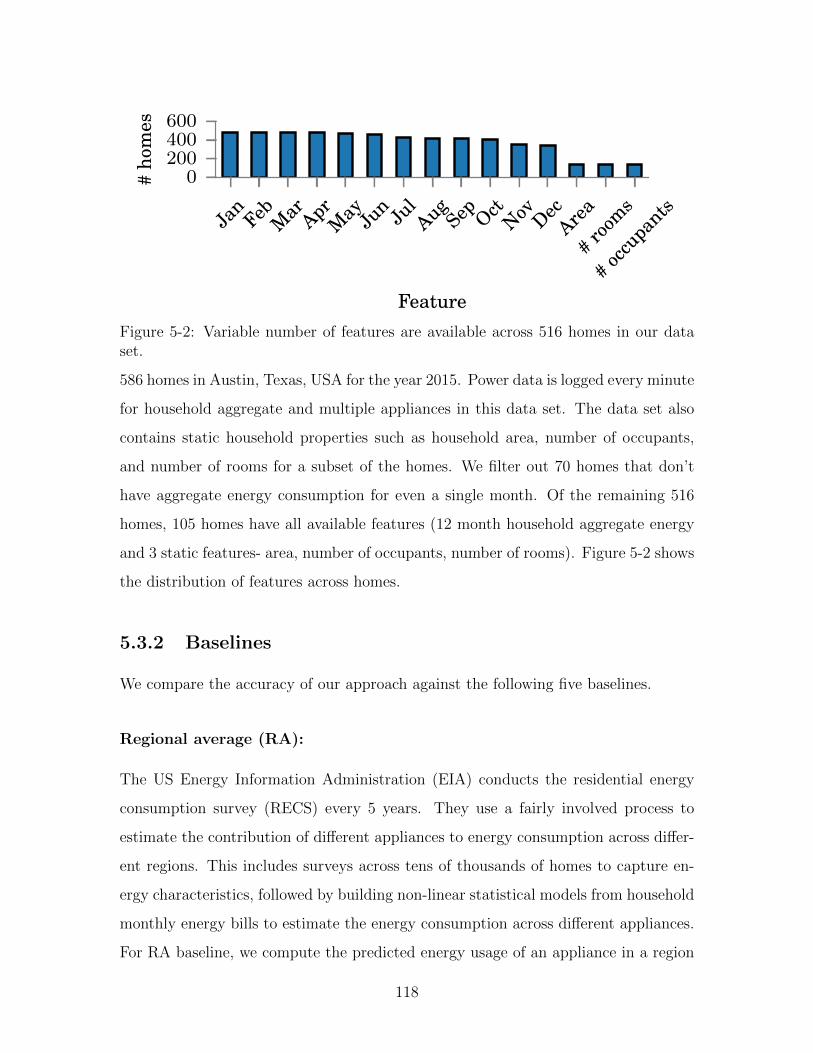
Jan

Feb Mar Apr

May Ju

n Jul

AugSep Oct

Nov DecAre

a

# room

s

# occu

pants

Feature

0200400600

#ho

mes

Figure 5-2: Variable number of features are available across 516 homes in our dataset.

586 homes in Austin, Texas, USA for the year 2015. Power data is logged every minute

for household aggregate and multiple appliances in this data set. The data set also

contains static household properties such as household area, number of occupants,

and number of rooms for a subset of the homes. We filter out 70 homes that don’t

have aggregate energy consumption for even a single month. Of the remaining 516

homes, 105 homes have all available features (12 month household aggregate energy

and 3 static features- area, number of occupants, number of rooms). Figure 5-2 shows

the distribution of features across homes.

5.3.2 Baselines

We compare the accuracy of our approach against the following five baselines.

Regional average (RA):

The US Energy Information Administration (EIA) conducts the residential energy

consumption survey (RECS) every 5 years. They use a fairly involved process to

estimate the contribution of different appliances to energy consumption across differ-

ent regions. This includes surveys across tens of thousands of homes to capture en-

ergy characteristics, followed by building non-linear statistical models from household

monthly energy bills to estimate the energy consumption across different appliances.

For RA baseline, we compute the predicted energy usage of an appliance in a region

118

as the product of the regional average proportion of that appliance and the aggregate

monthly energy consumption of the home.

NILM- FHMM, LBM and DDSC:

We use three NILM techniques as baselines. We use a factorial hidden Markov model

(FHMM) [41, 73], which is accepted as a gold standard in NILM literature. In an

FHMM, each appliance is modelled as a Gaussian hidden Markov model, containing

three parameters: prior, transition matrix and emission matrix. Each appliance is

modelled to contain S states (such as ON, OFF, etc.). The prior encodes the initial

probability of an appliance starting in different states ({1..S}). The transition matrix

encodes the probability of transition from state si to sj. The emission matrix encodes

the distribution of power for different states.

We use the state-of-the-art NILM technique based on latent bayesian melding (LBM) [107,

105] proposed by Zhong et. al, as our second NILM benchmark. The goal of this

work by Zhong et. al is to break down the energy consumption into appliances given

the aggregate power time series . The underlying model used in this approach is an

FHMM. In addition to modelling the system as an FHMM, the authors in this work

add prior constraints to improve the accuracy. An example of such constraints is

the expected number of ON/OFF transitions of an appliance. We use discrimina-

tive disaggregation sparse coding (DDSC) [72] as the third NILM baseline. DDSC

is based upon structured prediction for discriminatively training sparse coding algo-

rithms specifically to maximise disaggregation performance.

All these three NILM technique produce a high frequency time series for different

appliances and we sum up the energy consumption to obtain per-appliance monthly

energy consumption.

Gemello/kNN

We use Gemello [20] as our final baseline. Gemello in its direct form is applicable

only to homes having all features and thus we can apply this baseline to the subset of

homes satisfying this constraint. For the remaining homes, having a variable number

119

of features, we use kNN where distances between homes are calculated based on

common set of features. It must be pointed that we could have alternatively imputed

the missing entries and used Gemello. We keep such an analysis for the future.

5.3.3 Implementation of our approach

The optimisation proposed for our approach proposed in Equation 5.2 is not jointly

convex in A and B. However, by fixing one, the optimisation becomes convex in the

other. Thus, we implement an alternating least square (ALS) strategy implemented

in Python using CVXPY [33]. CVXPY also allows us to specify the non-negative

constraints and incorporating static features. Another important implementation

detail involves linearly normalising the matrix entries on a scale of 0 to 1 by using

the maximum and the minimum entry in the matrix.

5.3.4 Evaluation metric

We chose our metric after deliberating on the metrics used in prior work and our

discussions with NILM experts. Since different appliances are on a different scale

(HVAC consumes significantly more energy than a microwave), comparing the RMS

error in energy consumption can be hard to interpret across appliances. Normalising

the error by actual usage may seem a possible solution. However, this metric breaks

for low-energy appliances. For example, if the actual and predicted usage of the oven is

0.1 and 0.2 units, error would be 100%. However, an error of 0.1 units would probably

be insignificant in absolute terms. To overcome the problems of the above two metrics,

we choose a metric defined as RMS error in percentage of energy correctly assigned

(PEC) [16], where, PEC for the home, appliance, month (< h,w,m >) triplet is

given by:

PEC(h,w,m) =|wprediction(h,m)− w(h,m)|

aggregate(h,m)× 100% (5.3)

where w(h,m) denotes the ground truth energy usage by appliance w in home h

in month m and aggregate(h,m) denotes the ground truth aggregate home energy

usage for home h in month m. The RMS error in the percentage of energy correctly

120

HVAC Fridge Washing machine Dishwasher

0.29 0.09 0.01 0.02

Table 5.1: Proportion of energy consumed by different appliances in Austin.

assigned (PEC), for an appliance w is given as the RMS of PEC(h,w,m) across

different months and homes. Lower RMS error in percentage of energy correctly

assigned (PEC) means better prediction.

5.3.5 Experimental setup

We perform our analysis on six appliances - heating, ventilation and air-conditioning

(HVAC), fridge, washing machine (WM), microwave (MW), dish washer (DW) and

oven. There are three main reasons for choosing these six appliances. First, our data

set contains a substantial number of homes with these 6 appliances. Second, these

six appliances represent a diverse category: i) HVAC represents appliances that are

heavily affected by weather and consume high energy, ii) fridge represents always

ON appliances, that are moderately affected by weather and usage, iii) washing ma-

chine and dryer represents appliances that are highly usage dependent and typically

consume low energy relative to HVAC and fridge, oven and microwave represent ap-

pliances used in the kitchen. Third, together these six appliances contribute more

than half of the total household energy. We perform our evaluation on two different

test sets- 105 homes having all feature and 516 homes containing homes with missing

features.

For regional average (RA) baseline, we use the numbers obtained from RECS survey

as shown in Table 5.1. It must be noted that the RECS survey doesn’t have appliance

level numbers for oven and microwave, and we thus can’t make a prediction for these

two appliances using RA baseline.

For our FHMM and LBM baselines, we use their implementation in NILMTK [16]

and model each appliance as a 3-state appliance (Off, Intermediate and High power),

as per the work in [107]. To measure the NILM performance given current smart

meters, we feed the NILM algorithm 15-minute aggregate reading which it tries to

break down into 15-minute time series for the six appliances. The NILM model is

121

trained on the entire 516 homes including the test homes as we wanted to see the best

performance of baseline algorithms. Due to time constraints, we were able to evaluate

the performance of DDSC only over the 105 homes having all features. DDSC was

inputted 15-minute appliance and aggregate power traces for training and 15-minute

home aggregate power traces for testing. Optimal parameters for DDSC were learnt

using cross-validation. The three NILM approaches produce as output a 15-minute

power time series for each appliance which is aggregated to monthly appliance energy

consumption. It must be mentioned that while the LBM implementation comes from

the authors of that paper, the FHMM one comes from a publicly available toolkit,

the implementation of DDSC is ours and thus may not fully match with the authors’

version.

Gemello has top-N features and number of neighbours K as tunable parameters. For

Gemello, we use the parameters used in previous work [20], K varies from 1 to 6, and

N varies from 1 to 8.

Our MF based approach has regularisation (λ), static features to include (area, num-

ber of occupants and number of rooms) and the number of latent factors as the

tunable parameters. We varied λ in factors of 10 from 10−3 to 102. We used

all length-0, 1, 2 and 3 combinations of the 3 static features (<None>, <area>,

<#occupants>,. . .<area, #occupants, #rooms>). We varied the number of latent

factors from 1 to 10. We chose to set 10 as the upper limit on the number of latent

factors as we have data from 12 months, and we would want a low-rank approxima-

tion.

For both Gemello and MF, we use a nested leave-one-out cross-validation strategy.

The inner loop is used to fine-tune the parameters. The outer loop is used for pre-

diction of energy across different appliances for a test home, when all but that home

are used in the train set. It must be pointed out that both Gemello and our MF ap-

proach have the same set of input information available (historical aggregate energy

and appliance montly energy consumption, and three static household properties).

Our entire implementation, experiments and analysis can be found on Github (URL

not mentioned for anonymity).

122

FHMM LBM DDSC RA Gemello MF

HVAC 15.26 29.37 31.39 17.44 12.62 12.53

Fridge 4.48 2.69 4.32 4.62 4.37 3.65

Oven 34.09 3.84 1.37 - 1.07 1.04

DW 12.99 1.74 1.30 1.22 1.05 0.92

WM 3.98 13.29 1.36 0.71 0.50 0.49

MW 6.32 1.01 1.08 - 0.87 0.64

Table 5.2: RMS error (lower is better) in the percentage of energy assigned for 105homes having all features.

FHMM LBM RA KNN MF

HVAC 15.65 29.37 18.40 11.96 12.02

Fridge 3.90 2.69 4.41 3.38 3.62

Oven 34.00 3.84 - 1.49 1.32

DW 13.80 1.74 1.22 1.01 0.92

WM 3.89 13.29 1.40 1.45 1.33

MW 5.76 1.01 - 0.98 0.91

Table 5.3: RMS error (lower is better) in the percentage of energy assigned for 516homes (having missing features).

5.3.6 Results and Analysis

Our main result in Table 5.2 on 105 homes having all features, shows that our MF

approach gives better energy breakdown performance than the four baselines for 5/6

appliances. The relative improvement in energy breakdown performance over the

best baseline, is the highest for microwave and dish washer. Both these appliances

are generally considered problematic for traditional NILM algorithms [7] owing to

their multiple states of operation and in general sparse usage. For the fridge, LBM

gives best performance followed by our approach. This may be due to the fact that

LBM is accurately able to balance the prior (expected number of cycle and energy

usage) with the time series data for the fridge. Other appliances may not be showing

such cyclic behaviour.

In Table 5.3, we see that our MF approach gives better energy breakdown performance

than the four baselines for 4/6 appliances for 516 homes. As we saw before, LBM does

best for the fridge. For HVAC, while KNN gives the best performance, our approach

123

0.04 0.06 0.08 0.10 0.12 0.14 0.16 0.18 0.20 0.22

Latent factor for months

300

400

500

600

700

800

#D

egre

eda

ys

May

Jun

JulAug

Sep

Oct

Figure 5-3: One of the latent factors learnt for HVAC has a high correlation with the# of degree days

is comparable.

We now analyse the efficacy of our MF based approach on the data from 105 homes.

When learning latent factors for HVAC, we found one of the factors for month to

be highly correlated with the air conditioning requirement for that month (Figure

5-3). The air conditioning requirement for a month can be captured by a parameter

called the number of degree days4. Since the HVAC energy consumption is seasonal

and depends on the number of degree days, our approach is expected to work better

than baselines (including KNN), which aren’t able to capture such information. On

a similar front, when we did MF without explicitly incorporating static features,

we found that some of the latent factors had a high correlation with these static

parameters. Figure 5-4 shows the relative gain in performance by the addition of these

static features over the standard MF. While all appliances show an improvement in

performance by the addition of static features, dish washer has the maximum gain.

This is consistent with previous similar work [20], which shows that static features

are useful for appliances such as dish washer.

We further tried to answer the question- “What’s better? More, but incomplete data,

or, less but complete data”. For this, we use all the 516 homes for training and anal-

ysed the performance of the test 105 homes having all features, compared to training

only on these 105 homes. Our results in Figure 5-4 show that for 4/6 appliances, the

4https://en.wikipedia.org/wiki/Degree_day

124

HVAC

Fridge

Oven

DWW

MM

W

−5

0

5

10

15R

elat

ive

%re

duct

ion

iner

ror

MF-105 homes, featureMF-516 homes

MF-516 homes, feature

Figure 5-4: Reduction in error over MF on 105 homes over 6 appliances. Incorporatingstatic features into our matrix factorisation improves energy breakdown performance.

performance improves by adding more homes and performing plain MF (without ad-

ditional features). When static features are also considered, there is an improvement

in performance for all the 6 appliances. While this data may not be sufficient for

conclusively saying that more data is better, the case for the value of static features

is more conclusive.

5.4 Implementation For Scale

We now discuss an implementation of our system which can scale to millions of homes

across the US. The US Energy department runs a program called Green Button,

under which, more than 50 utilities across the US are allowing 60 million households

to download their energy consumption in a standard format. This program caters

to users having smart meters and traditional electricity meters. We have created a

web application where users can upload their Green Button data to obtain their per-

appliance energy breakdown, which we obtain by applying our approach on existing

data sets having appliance level data. To obtain household static properties, we

request the users for their address and can pull information such as household area

125

Figure 5-5: Screenshot from the web user interface that can potentially provide energybreakdown to millions of homes in the US leveraging our approach.

and age from online APIs such as the one offered by Zillow5. Figure 5-5 shows a

screenshot from an initial prototype.

5.5 Discussion

We now discuss two additional properties and insights that can be incorporated into

our approach that we did not consider due to space and time constraints. Previous

work has shown that energy breakdown performance can be improved by incorpo-

rating correlation of appliances with seasonal weather data[102] and the correlation

between appliances [68]. We believe that such domain insights can be captured in the

MF formulation.

1. Temporal characteristics: We can categorise household appliances into those

affected (e.g. HVAC) or not affected (e.g. oven) by seasonal trends. For appliances

not affected by seasonal changes, we can impose a penalty on variation in predicted

energy consumption across months. The penalty can be imposed by adding the

5http://bit.ly/1PWZGOp

126

following term to Equation 5.1:

Min ¯k∑

i=1

2n−1∑j=1

(B[i, j + 1]−B[i, j])2,where ¯ > 0 (5.4)

This term smoothes B, and thus poses a penalty on variation in energy of appliance

across months.

For appliances that are affected by seasonal variations, we can explicitly add proper-

ties capturing seasonal variations (such as temperature) as known latent factors for

B [102].

2. Appliance correlations: The energy usage of different appliances is often corre-

lated [68]. For example, the energy usage of a dryer is likely to be correlated with the

washing machine. This property can be captured by constructing a matrix structure

containing all the correlated appliances as well as aggregate energy. The latent factors

can be constrained in a similar fashion as we did in Equation 5.4.

5.6 Summary

Energy breakdown literature has largely looked at methods that require additional

hardware to be installed. Due to prohibitive costs, it is unlikely that a significant

proportion of the world will have access to such hardware. We presented a simple

matrix factorisation based approach that does not require any sensing in the test

home. Our approach presents an interesting dimension to the well-studied problem

and owing to the no additional hardware nature, is likely to be easier to scale. All

the infrastructure required to scale such an approach already exists. The efficacy of

our approach is shown by its competitiveness against state-of-the-art NILM methods

that rely on additional hardware.

127

128

Chapter 6

Conclusions and Future Work

The field of NILM or energy breakdown is more than three decades old. During these

three decades, loads of new algorithmic approaches have been proposed. Many start-

up companies have leveraged energy breakdown techniques in some of their offerings.

However, there were three factors impeding practicality of energy breakdown- lack of

comparability, action-ability and scalability. We now conclude our thoughts across

these dimensions and also suggest future work.

6.1 Ensuring comparison across approaches

6.1.1 Conclusions

When we began our NILM work, we wanted to use the “best” NILM algorithm and

develop applications on top. We realised that finding the “best” NILM algorithm was

no trivial task. Different researchers had used different data sets, different benchmark

algorithms and different metrics. This made it virtually impossible to compare NILM

papers and ascertain the best NILM algorithm. At this point we felt our efforts would

be best spent towards making NILM research more standardised. This was also the

general consensus of the community as discussed in the NILM workshop. One of

our goals was to lower the entry barrier for NILM researchers. We teamed up with

researchers from the UK and the US to develop the NILM toolkit. In our experience,

129

all the engineering effort spent in NILMTK, paid us back many times in terms of

research output. We are very satisfied that beyond the core developers, NILMTK

has been used by the community. Researchers have contributed their algorithms and

data sets to NILMTK.

6.1.2 Future work

1. Despite the positive traction gained by NILMTK, still a vast amount of lit-

erature remains hard to compare against. While NILMTK is an important

first step towards making NILM algorithms more comparable, significant ef-

forts are needed towards the goal. The image processing community serves as

a good example of comparable scientific research. The ImageNet challenge1

can be attributed to a lot of recent comparable state-of-the-art work in the

field. We believe that the energy breakdown community would similarly benefit

from such a competition. In fact, one of the NILMTK’s lead developers, Jack

Kelly2, is currently pursuing this thread. There are several other ways in which

the community can help, such as mandating code release for any submission.

Many conferences encourage code submission for paper submissions. Integrat-

ing a Kaggle-like3 service for standardised tasks (similar to the competition)

can greatly help in making the field more standardised. The community will

also benefit by integrating their open tools with tools such as NILMTK. An

example is a recent household energy simulator called SmartSim [24].

2. While we compared the NILM problem to the image processing problem, which

has the ImageNet challenge, there are few important differences. Different

NILM researchers focus on different frequency of data collection. The frequency

range is huge- ranging from a sample every 15 minutes, to millions of samples

every second. NILMTK in its current form is tuned to low frequency data col-

lection. In fact, till date it remains nearly impossible to compare the efficacy

1http://image-net.org/2http://jack-kelly.com/3https://www.kaggle.com/

130

of low-frequency approaches against the high-frequency approaches. This is

due to the fact that very few current data sets measure both low-frequency and

high-frequency power data, and tools like NILMTK have not been developed for

high-frequency data. Future datasets collection should account for such high-

frequency and low-frequency parallel data collection so as to support diverse

comparison.

6.2 From disaggregation to specific actions

6.2.1 Conclusions

After our NILMTK work, we were faced with two choices - build more accurate NILM

algorithms, or, work towards our initial aim, to save energy. The “usefulness” of NILM

had also been questioned many times. Thus, we undertook research to understand

if energy breakdown can provide specific actionable energy saving insights, over and

above the pie-chart energy breakdown. There were two important questions that we

needed to answer the applicability of NILM research. First, can we leverage appliance

power traces to provide actionable insights? Second, do current NILM approaches

provide disaggregated appliance traces with sufficient fidelity to facilitate actionable

energy saving insights?

To answer the first question on the utility of appliance level power traces towards

actionable energy savings, we need to construct appliance energy models. These ap-

pliance energy models should be able to distinguish regular and anomalous operation

of the appliance. Based on models and insights developed by domain experts, we

created simple models for fridge and HVAC. Our key idea was to use these models

to provide insights such as -“your HVAC is set to a wrong temperature, this rec-

ommended schedule can save you 10% on your bills”. Our findings indicate that

energy saving insights can save up to a quarter of the appliance energy consumption.

However, when we investigated the appliance level traces provided by NILM algo-

rithms, we found that the appliance traces produced by current NILM algorithms

131

show poor feedback accuracy. The same NILM algorithms show good accuracy on

conventional NILM metrics such as F1 scores and RMS error. This can be explained

by the fact that NILM algorithms do well in general, giving good performance on

conventional metrics. But, the cases we care about for appliance feedback are often

poorly predicted. Our work suggests that the community take an alternative view of

the problem where actionability is a key concern. This would entail development of

algorithms with the new set of metrics (focusing on applications).

6.2.2 Future work

We illustrated actionable feedback for two appliances - fridge and HVAC. A large

number of appliance categories still need to be covered. In fact, our current approach

of manually creating a white-box model for each appliance category may not scale

particularly well. One approach could be to develop energy models for classes of ap-

pliances, such as - thermostatically controlled, purely resistive, switched-mode based

power supply among others. Another possible direction is the development of smart

appliances that incorporate actuation capabilities and local intelligence for optimal

appliance operation. With the advent of NEST and similar smart appliances, the con-

trol and intelligence are increasingly being pushed to the end device. This is where

our work could fit well into products. These smart appliances can run algorithms

similar to ours and inform the appliance owners about inefficient usage.

6.3 Scaling up energy breakdown

6.3.1 Conclusions

We realised that a great deal of energy breakdown literature could not be scaled today

to all homes. This is due to the fact that current energy breakdown solutions require

hardware to be installed in each home. Even though smart meters have been rolled

out across the US, these smart meters often sample at low rates, which makes most

of the NILM literature impertinent. Against this background, we chose to develop

132

scalable energy breakdown solutions that do not require any hardware to be installed

in a test home. We started with the goal of creating an energy breakdown solution

that works with whatever data is easily accessible, is able to scale across a large num-

ber of homes and requires minimal capital expenditure involved. In order to achieve

these objectives, we completely flipped the way we look at the problem. Rather than

the existing bottom-up approach of using modelling to identify electrical signatures,

we used the top-down approach of using modelling to identify home level character-

istics that correlate well with appliance level energy consumption. We showed that

such home level characteristics can be easily calculated with static household infor-

mation and monthly electricity data both of which are readily available. Not only

is our approach more scalable, it is also more accurate than state-of-the-art NILM

approaches.

6.3.2 Future work

1. Our approach currently faces the challenge of the availability of static informa-

tion (metadata) along with the power data. Very few public data sets survey

such information. Future data set owners should try and obtain as much static

household properties as possible. Other NILM approaches have also shown the

benefit of such metadata. Our current work on making energy breakdown more

scalable works only for homes in the same geographical regions. If we can learn

the properties of different regions that cause differences in energy consumption,

we can make energy breakdown more scalable. We are currently looking into

transfer learning methods for scaling energy breakdown across multiple geogra-

phies.

2. The first step towards realising some of the associated benefits from scalable

energy breakdown would be to carry out pilot deployments where people are

given the energy breakdown estimated by our system. Such large-term studies

are needed to truly understand the impact of our technology at scale.

133

134

Bibliography

[1] Buildings and climate change. http://www.eesi.org/files/climate.pdf.Accessed: 2016-10-24.

[2] Global climate change: Vital signs of the planet. http://climate.nasa.gov/.Accessed: 2016-09-30.

[3] Yuvraj Agarwal, Rajesh Gupta, Daisuke Komaki, and Thomas Weng. Build-ingdepot: an extensible and distributed architecture for building data storage,access and sharing. In Proceedings of the Fourth ACM Workshop on EmbeddedSensing Systems for Energy-Efficiency in Buildings, pages 64–71. ACM, 2012.

[4] Kyle Anderson, Adrian Ocneanu, Diego Benitez, Derrick Carlson, AnthonyRowe, and Mario Berges. BLUED: A fully labeled public dataset for Event-Based Non-Intrusive load monitoring research. In Proceedings of 2nd KDDWorkshop on Data Mining Applications in Sustainability, pages 12–16, Beijing,China, 2012.

[5] Pandarasamy Arjunan, Nipun Batra, Haksoo Choi, Amarjeet Singh, Pushpen-dra Singh, and Mani B Srivastava. Sensoract: a privacy and security awarefederated middleware for building management. In Proceedings of the FourthACM Workshop on Embedded Sensing Systems for Energy-Efficiency in Build-ings, pages 80–87. ACM, 2012.

[6] K Carrie Armel, Abhay Gupta, Gireesh Shrimali, and Adrian Albert. Is dis-aggregation the holy grail of energy efficiency? The case of electricity. EnergyPolicy, 52:213–234, 2013.

[7] Sean Barker, Sandeep Kalra, David Irwin, and Prashant Shenoy. Empiricalcharacterization and modeling of electrical loads in smart homes. In IEEEIGCC, Arlington, VA, USA, 2013.

[8] Sean Barker, Sandeep Kalra, David Irwin, and Prashant Shenoy. Nilm redux:The case for emphasizing applications over accuracy. In NILM-2014 Workshop,2014.

[9] Sean Barker, Sandeep Kalra, David Irwin, and Prashant Shenoy. Powerplay:creating virtual power meters through online load tracking. In Proceedings ofthe 1st ACM Conference on Embedded Systems for Energy-Efficient Buildings,pages 60–69. ACM, 2014.

135

[10] Sean Barker, Aditya Mishra, David Irwin, Emmanuel Cecchet, PrashantShenoy, and Jeannie Albrecht. Smart*: An open data set and tools for en-abling research in sustainable homes. In Proceedings of 2nd KDD Workshop onData Mining Applications in Sustainability, Beijing, China, 2012.

[11] Sean Barker, Aditya Mishra, David Irwin, Prashant Shenoy, and Jeannie Al-brecht. Smartcap: Flattening peak electricity demand in smart homes. In Per-vasive Computing and Communications (PerCom), 2012 IEEE InternationalConference on, pages 67–75. IEEE, 2012.

[12] Nipun Batra, Pandarasamy Arjunan, Amarjeet Singh, and Pushpendra Singh.Experiences with occupancy based building management systems. In Intelli-gent Sensors, Sensor Networks and Information Processing, 2013 IEEE EighthInternational Conference on, pages 153–158. IEEE, 2013.

[13] Nipun Batra, Rishi Baijal, Amarjeet Singh, and Kamin Whitehouse. How goodis good enough? re-evaluating the bar for energy disaggregation. arXiv preprintarXiv:1510.08713, 2015.

[14] Nipun Batra, Haimonti Dutta, and Amarjeet Singh. Indic: Improved non-intrusive load monitoring using load division and calibration. In MachineLearning and Applications (ICMLA), 2013 12th International Conference on,volume 1, pages 79–84. IEEE, 2013.

[15] Nipun Batra, Manoj Gulati, Amarjeet Singh, and Mani B. Srivastava. It’sDifferent: Insights into home energy consumption in India. In Proceedings ofthe Fifth ACM Workshop on Embedded Sensing Systems for Energy-Efficiencyin Buildings, 2013.

[16] Nipun Batra, Jack Kelly, Oliver Parson, Haimonti Dutta, William Knottenbelt,Alex Rogers, Amarjeet Singh, and Mani Srivastava. NILMTK: An Open SourceToolkit for Non-intrusive Load Monitoring. In Fifth International Conferenceon Future Energy Systems, Cambridge, UK, 2014.

[17] Nipun Batra, Oliver Parson, Mario Berges, Amarjeet Singh, and Alex Rogers.A comparison of non-intrusive load monitoring methods for commercial andresidential buildings. arXiv preprint arXiv:1408.6595, 2014.

[18] Nipun Batra, Amarjeet Singh, Pushpendra Singh, Haimonti Dutta, VenkateshSarangan, and Mani Srivastava. Data driven energy efficiency in buildings.arXiv preprint arXiv:1404.7227, 2014.

[19] Nipun Batra, Amarjeet Singh, and Kamin Whitehouse. If you measure it, canyou improve it? exploring the value of energy disaggregation. In Proceedings ofthe second ACM International Conference on Embedded Systems For Energy-Efficient Built Environments. ACM, 2015.

136

[20] Nipun Batra, Amarjeet Singh, and Kamin Whitehouse. Gemello: Creating adetailed energy breakdown from just the monthly electricity bill. In SIGKDD2016, 2016.

[21] Nipun Batra, Hongning Wang, Amarjeet Singh, and Kamin Whitehouse. Matrixfactorisation for scalable energy breakdown. In AAAI 2017, 2017.

[22] Christian Beckel, Leyna Sadamori, and Silvia Santini. Automatic socio-economic classification of households using electricity consumption data. InProceedings of the fourth international conference on Future energy systems,pages 75–86. ACM, 2013.

[23] California Public Utilities Commission. Final Opinion Authorizing Pacific Gasand Electric Company to Deploy Advanced Metering Infrastructure. Technicalreport, 2006.

[24] Dong Chen, David Irwin, and Prashant Shenoy. Smartsim: A device-accuratesmart home simulator for energy analytics.

[25] Ke-Yu Chen, Sidhant Gupta, Eric C Larson, and Shwetak Patel. Dose: De-tecting user-driven operating states of electronic devices from a single sensingpoint. In Pervasive Computing and Communications (PerCom), 2015 IEEEInternational Conference on, pages 46–54. IEEE, 2015.

[26] Victor L Chen, Magali A Delmas, William J Kaiser, and Stephen L Locke. Whatcan we learn from high-frequency appliance-level energy metering? results froma field experiment. Energy Policy, 77:164–175, 2015.

[27] Meghan Clark, Bradford Campbell, and Prabal Dutta. Deltaflow: submeteringby synthesizing uncalibrated pulse sensor streams. In Proceedings of the 5thinternational conference on Future energy systems. ACM, 2014.

[28] Mark Costanzo, Dane Archer, Elliot Aronson, and Thomas Pettigrew. Energyconservation behavior: The difficult path from information to action. Americanpsychologist, 41(5):521, 1986.

[29] Sarah Darby. The effectiveness of feedback on energy consumption. A Reviewfor DEFRA of the Literature on Metering, Billing and direct Displays, 2006.

[30] Stephen Dawson-Haggerty, Xiaofan Jiang, Gilman Tolle, Jorge Ortiz, and DavidCuller. smap: a simple measurement and actuation profile for physical infor-mation. In Proceedings of the 8th ACM Conference on Embedded NetworkedSensor Systems, pages 197–210. ACM, 2010.

[31] Samuel DeBruin, Branden Ghena, Ye-Sheng Kuo, and Prabal Dutta.Powerblade: A low-profile, true-power, plug-through energy meter. In Pro-ceedings of the 13th ACM Conference on Embedded Networked Sensor Systems,pages 17–29. ACM, 2015.

137

[32] Department of Energy & Climate Change. Smart Metering Equipment Techni-cal Specifications Version 2. Technical report, UK, 2013.

[33] Steven Diamond and Stephen Boyd. Cvxpy: A python-embedded modelinglanguage for convex optimization. Journal of Machine Learning Research, 2016.

[34] Roy J Dossat and Thomas J Horan. Principles of refrigeration, volume 3. Wiley,1961.

[35] Ehsan Elhamifar and Shankar Sastry. Energy disaggregation via learning ’pow-erlets’ and sparse coding. In Proceedings of the Twenty-Ninth AAAI Conferenceon Artificial Intelligence, AAAI’15, pages 629–635. AAAI Press, 2015.

[36] EnergyStar.gov. Programmable thermostats for consumers.

[37] Meredydd Evans, Bin Shui, and Sriram Somasundaram. Country report onbuilding energy codes in india. Pacific Northwest National Laboratory, 2009.

[38] Jon Froehlich, Eric Larson, Sidhant Gupta, Gabe Cohn, Matthew Reynolds,and Shwetak Patel. Disaggregated end-use energy sensing for the smart grid.

[39] Tanuja Ganu, Deva P Seetharam, Vijay Arya, Rajesh Kunnath, JagabondhuHazra, Saiful A Husain, Liyanage Chandratilake De Silva, and ShivkumarKalyanaraman. nplug: a smart plug for alleviating peak loads. In Proceed-ings of the 3rd International Conference on Future Energy Systems: WhereEnergy, Computing and Communication Meet, page 30, 2012.

[40] Jingkun Gao, Suman Giri, Emre Can Kara, and Mario Berges. Plaid: a publicdataset of high-resoultion electrical appliance measurements for load identifi-cation research: demo abstract. In proceedings of the 1st ACM Conference onEmbedded Systems for Energy-Efficient Buildings, pages 198–199. ACM, 2014.

[41] Zoubin Ghahramani and Michael I Jordan. Factorial hidden markov models.Machine learning, 29(2-3), 1997.

[42] Ary L Goldberger, Luis AN Amaral, Leon Glass, Jeffrey M Hausdorff, Pla-men Ch Ivanov, Roger G Mark, Joseph E Mietus, George B Moody, Chung-Kang Peng, and H Eugene Stanley. PhysioBank, PhysioToolkit, and PhysioNet:components of a new research resource for complex physiologic signals. Circu-lation, 101(23):e215–e220, 2000.

[43] Manoj Gulati, Shobha Sundar Ram, Angshul Majumdar, and Amarjeet Singh.Single point conducted emi sensor with intelligent inference for detecting itappliances. IEEE Transactions on Smart Grid, 2016.

[44] Manoj Gulati, Shobha Sundar Ram, and Amarjeet Singh. An in depth studyinto using emi signatures for appliance identification. In Proceedings of the 1stACM Conference on Embedded Systems for Energy-Efficient Buildings, pages70–79. ACM, 2014.

138

[45] Manoj Gulati, Vibhutesh Kumar Singh, Sanchit Kumar Agarwal, andVivek Ashok Bohara. Appliance activity recognition using radio frequency in-terference emissions. IEEE Sensors Journal, 16(16):6197–6204, 2016.

[46] Manoj Gulati, Shobha Sundar Ram, Angshul Majumdar, and Amarjeet Singh.Detecting it and lighting loads using common mode conducted emi signals. In3rd International Workshop on Non-Intrusive Load Monitoring, 2016.

[47] M. Gupta and A. Majumdar. Nuclear norm regularized robust dictionary learn-ing for energy disaggregation. In 2016 24th European Signal Processing Con-ference (EUSIPCO), pages 677–681, Aug 2016.

[48] Sidhant Gupta, Matthew S Reynolds, and Shwetak N Patel. Electrisense:single-point sensing using emi for electrical event detection and classificationin the home. In Ubicomp, 2010.

[49] Wouter J Den Haan and Andrew T Levin. A practitioner’s guide to robustcovariance matrix estimation, 1996.

[50] George William Hart. Nonintrusive appliance load monitoring. Proceedings ofthe IEEE, 80(12):1870–1891, 1992.

[51] Taha Hassan, Fahad Javed, and Naveed Arshad. An empirical investigationof vi trajectory based load signatures for non-intrusive load monitoring. IEEETransactions on Smart Grid, 5(2):870–878, 2014.

[52] Timothy W Hnat, Vijay Srinivasan, Jiakang Lu, Tamim I Sookoor, RaymondDawson, John Stankovic, and Kamin Whitehouse. The hitchhiker’s guide tosuccessful residential sensing deployments. In Proceedings of the 9th ACM Con-ference on Embedded Networked Sensor Systems, pages 232–245. ACM, 2011.

[53] Timothy W Hnat, Vijay Srinivasan, Jiakang Lu, Tamim I Sookoor, RaymondDawson, John Stankovic, and Kamin Whitehouse. The hitchhiker’s guide tosuccessful residential sensing deployments. In Proceedings of the 9th ACM Con-ference on Embedded Networked Sensor Systems, pages 232–245. ACM, 2011.

[54] C. Holcomb. Pecan Street Inc.: A Test-bed for NILM. In International Work-shop on Non-Intrusive Load Monitoring, Pittsburgh, PA, USA, 2012.

[55] Milan Jain. Data driven feedback for optimized and efficient usage of decen-tralized air conditioners. In Pervasive Computing and Communication Work-shops (PerCom Workshops), 2016 IEEE International Conference on, pages1–3. IEEE, 2016.

[56] Milan Jain and Amarjeet Singh. Pacman: predicting ac consumption minimiz-ing aggregate energy consumption. DSpace at IIIT-Delhi, 2014.

139

[57] Milan Jain, Amarjeet Singh, and Vikas Chandan. Non-intrusive estimation andprediction of residential ac energy consumption. In 2016 IEEE InternationalConference on Pervasive Computing and Communications (PerCom), pages 1–9. IEEE, 2016.

[58] Kathryn B Janda. Buildings don’t use energy: people do. Architectural sciencereview, 54(1):15–22, 2011.

[59] Xiaofan Jiang, Stephen Dawson-Haggerty, Prabal Dutta, and David Culler. De-sign and implementation of a high-fidelity ac metering network. In InformationProcessing in Sensor Networks, 2009. IPSN 2009. International Conference on,pages 253–264. IEEE, 2009.

[60] Amir Kavousian, Ram Rajagopal, and Martin Fischer. Determinants of resi-dential electricity consumption: Using smart meter data to examine the effectof climate, building characteristics, appliance stock, and occupants’ behavior.Energy, 55(0):184 – 194, 2013.

[61] Jack Kelly. Disaggregation of Domestic Smart Meter Energy Data. PhD thesis.

[62] Jack Kelly, Nipun Batra, Oliver Parson, Haimonti Dutta, William Knotten-belt, Alex Rogers, Amarjeet Singh, and Mani Srivastava. Nilmtk v0. 2: anon-intrusive load monitoring toolkit for large scale data sets: demo abstract.In Proceedings of the 1st ACM Conference on Embedded Systems for Energy-Efficient Buildings, pages 182–183. ACM, 2014.

[63] Jack Kelly and William Knottenbelt. Metadata for Energy Disaggregation.In The 2nd IEEE International Workshop on Consumer Devices and Systems(CDS 2014), Vasteras, Sweden, July 2014.

[64] Jack Kelly and William Knottenbelt. UK-DALE: A dataset recording UK Do-mestic Appliance-Level Electricity demand and whole-house demand. ArXive-prints, 2014.

[65] Jack Kelly and William Knottenbelt. Neural nilm: Deep neural networks ap-plied to energy disaggregation. arXiv preprint arXiv:1507.06594, 2015.

[66] Jack Kelly and William Knottenbelt. Does disaggregated electricity feedbackreduce domestic electricity consumption? a systematic review of the literature.In 3rd International NILM Workshop, 2016.

[67] Willett Kempton and Laura Montgomery. Folk quantification of energy. Energy,7(10):817–827, 1982.

[68] H. Kim, M. Marwah, M. F. Arlitt, G. Lyon, and J. Han. Unsupervised Dis-aggregation of Low Frequency Power Measurements. In Proceedings of 11thSIAM International Conference on Data Mining, pages 747–758, Mesa, AZ,USA, 2011.

140

[69] Hyungsul Kim, Manish Marwah, Martin F Arlitt, Geoff Lyon, and Jiawei Han.Unsupervised disaggregation of low frequency power measurements. SIAM.

[70] Hyungsul Kim, Manish Marwah, Martin F Arlitt, Geoff Lyon, and Jiawei Han.Unsupervised disaggregation of low frequency power measurements. In SDM,volume 11, pages 747–758. SIAM, 2011.

[71] Younghun Kim, Thomas Schmid, Zainul M Charbiwala, and Mani B Srivastava.Viridiscope: design and implementation of a fine grained power monitoring sys-tem for homes. In Proceedings of the 11th international conference on Ubiquitouscomputing, pages 245–254. ACM, 2009.

[72] J. Z. Kolter, S. Batra, and A. Y. Ng. Energy Disaggregation via DiscriminativeSparse Coding. In NIPS 2010, Vancouver, BC, Canada, 2010.

[73] J. Z. Kolter and T. Jaakkola. Approximate Inference in Additive FactorialHMMs with Application to Energy Disaggregation. In Proceedings of the Inter-national Conference on Artificial Intelligence and Statistics, La Palma, CanaryIslands, 2012.

[74] J Zico Kolter and Matthew J Johnson. REDD: A public data set for energydisaggregation research. In Proceedings of 1st KDD Workshop on Data MiningApplications in Sustainability, San Diego, CA, USA, 2011.

[75] David Kotz and Tristan Henderson. Crawdad: A community resource for archiv-ing wireless data at dartmouth. Pervasive Computing, IEEE, 4(4):12–14, 2005.

[76] Daniel D Lee and H Sebastian Seung. Algorithms for non-negative matrixfactorization. In NIPS 2001, 2001.

[77] Yucheng Low, Joseph Gonzalez, Aapo Kyrola, Danny Bickson, Carlos Guestrin,and Joseph M. Hellerstein. Graphlab: A new parallel framework for machinelearning. In Conference on Uncertainty in Artificial Intelligence, Catalina Is-land, CA, USA, 2010.

[78] Jiakang Lu, Tamim Sookoor, Vijay Srinivasan, Ge Gao, Brian Holben, JohnStankovic, Eric Field, and Kamin Whitehouse. The smart thermostat: usingoccupancy sensors to save energy in homes. In Proceedings of the 8th ACMConference on Embedded Networked Sensor Systems. ACM, 2010.

[79] A. Majumdar and R. Ward. Robust dictionary learning: Application to signaldisaggregation. In 2016 IEEE International Conference on Acoustics, Speechand Signal Processing (ICASSP), pages 2469–2473, March 2016.

[80] Stephen Makonin, Fred Popowich, Ivan V Bajic, Bob Gill, and Lyn Bartram.Exploiting hmm sparsity to perform online real-time nonintrusive load moni-toring.

141

[81] Stephen Makonin, Fred Popowich, Lyn Bartram, Bob Gill, and Ivan V. Bajic.AMPds: A Public Dataset for Load Disaggregation and Eco-Feedback Research.In IEEE Electrical Power and Energy Conference, Halifax, NS, Canada, 2013.

[82] Mary Meeker. Internet trends at stanford bases. KPCB, 2012.

[83] Oliver Parson. Unsupervised training methods for non-intrusive appliance loadmonitoring from smart meter data. PhD thesis, University of Southampton,2014.

[84] Oliver Parson, Grant Fisher, April Hersey, Nipun Batra, Jack Kelly, AmarjeetSingh, William Knottenbelt, and Alex Rogers. Dataport and nilmtk: A buildingdata set designed for non-intrusive load monitoring. In Third IEEE GlobalConference on Signal and Information Processing.

[85] Oliver Parson, Grant Fisher, April Hersey, Nipun Batra, Jack Kelly, AmarjeetSingh, William Knottenbelt, and Alex Rogers. Dataport and nilmtk: A buildingdata set designed for non-intrusive load monitoring. In GlobalSIP 2015. IEEE,2015.

[86] Oliver Parson, Siddhartha Ghosh, Mark Weal, and Alex Rogers. Non-intrusiveload monitoring using prior models of general appliance types. In AAAI 2012,Toronto, ON, Canada, 2012.

[87] Oliver Parson, Siddhartha Ghosh, Mark Weal, and Alex Rogers. An unsuper-vised training method for non-intrusive appliance load monitoring. ArtificialIntelligence, 217:1–19, 2014.

[88] F. Pedregosa, G. Varoquaux, A. Gramfort, V. Michel, B. Thirion, O. Grisel,M. Blondel, P. Prettenhofer, R. Weiss, V. Dubourg, J. Vanderplas, A. Passos,D. Cournapeau, M. Brucher, M. Perrot, and E. Duchesnay. Scikit-learn: Ma-chine learning in Python. Journal of Machine Learning Research, 12:2825–2830,2011.

[89] Luis Perez-Lombard, Jose Ortiz, and Christine Pout. A review on buildingsenergy consumption information. Energy and buildings, 40(3):394–398, 2008.

[90] Steffen Rendle, Zeno Gantner, Christoph Freudenthaler, and Lars Schmidt-Thieme. Fast context-aware recommendations with factorization machines. InProceedings of the 34th international ACM SIGIR conference on Research anddevelopment in Information Retrieval, pages 635–644. ACM, 2011.

[91] Richard de Dear and Melissa Hart. Appliance Electricity End-Use: Weather andClimate Sensitivity. Technical report, Sustainable Energy Group, AustralianGreenhouse Office, 2002.

[92] Alex Rogers, Siddhartha Ghosh, Reuben Wilcock, and Nicholas R Jennings.A scalable low-cost solution to provide personalised home heating advice to

142

households. In Proceedings of the 5th ACM Workshop on Embedded SystemsFor Energy-Efficient Buildings, pages 1–8. ACM, 2013.

[93] A Schoofs, A Guerrieri, D T Delaney, G O’Hare, and A G Ruzzelli. ANNOT:Automated Electricity Data Annotation Using Wireless Sensor Networks. InProceedings of the 7th Annual IEEE Communications Society Conference onSensor Mesh and Ad Hoc Communications and Networks, Boston, MA, USA,2010.

[94] Huijuan Shao, Manish Marwah, and Naren Ramakrishnan. A temporal motifmining approach to unsupervised energy disaggregation: Applications to resi-dential and commercial buildings.

[95] Shikha Singh and Angshul Majumdar. Deep sparse coding for non-intrusiveload monitoring. IEEE Transactions on Smart Grid, 2017.

[96] Shravan Srinivasan, Arunchandar Vasan, Venkatesh Sarangan, and Anand Siva-subramaniam. Bugs in the freezer: Detecting faults in supermarket refrigerationsystems using energy signals. In Proceedings of the 2015 ACM Sixth Interna-tional Conference on Future Energy Systems, pages 101–110. ACM, 2015.

[97] Vijay Srinivasan, John Stankovic, and Kamin Whitehouse. Fixturefinder: dis-covering the existence of electrical and water fixtures. In IPSN, 2013.

[98] Lakshmi V Thanayankizil, Sunil Kumar Ghai, Dipanjan Chakraborty, andDeva P Seetharam. Softgreen: Towards energy management of green officebuildings with soft sensors.

[99] Cathy Turner, Mark Frankel, et al. Energy performance of leed for new con-struction buildings. New Buildings Institute, 4:1–42, 2008.

[100] Ying Wei, Yu Zheng, and Qiang Yang. Transfer knowledge between cities.

[101] M. Wytock and J. Zico Kolter. Contextually Supervised Source Separation withApplication to Energy Disaggregation. ArXiv e-prints, 2013.

[102] Matt Wytock and J Zico Kolter. Contextually supervised source separationwith application to energy disaggregation. In AAAI 2014. AAAI Press, 2014.

[103] M Zeifman and K Roth. Nonintrusive appliance load monitoring: Review andoutlook. IEEE Transactions on Consumer Electronics, 57(1):76–84, 2011.

[104] Mingjun Zhong, Nigel Goddard, and Charles Sutton. Signal aggregate con-straints in additive factorial hmms, with application to energy disaggregation.In Advances in Neural Information Processing Systems, pages 3590–3598, 2014.

[105] Mingjun Zhong, Nigel Goddard, and Charles Sutton. Signal aggregate con-straints in additive factorial hmms, with application to energy disaggregation.In NIPS 2014, 2014.

143

[106] Mingjun Zhong, Nigel Goddard, and Charles Sutton. Latent bayesian meld-ing for integrating individual and population models. In Advances in NeuralInformation Processing Systems, pages 3618–3626, 2015.

[107] Mingjun Zhong, Nigel Goddard, and Charles Sutton. Latent bayesian meldingfor integrating individual and population models. In NIPS 2015, 2015.

[108] Jean-Paul Zimmermann, Matt Evans, Jonathan Griggs, Nicola King, Les Hard-ing, Penelope Roberts, and Chris Evans. Household Electricity Survey. A studyof domestic electrical product usage. Technical Report R66141, DEFRA, May2012.

[109] Ahmed Zoha, Alexander Gluhak, Muhammad Ali Imran, and Sutharshan Ra-jasegarar. Non-intrusive load monitoring approaches for disaggregated energysensing: A survey. Sensors, 12(12):16838–16866, 2012.

144