Systematic Derivation of Simplified Dynamics for … · Systematic Derivation of Simplified Dynamics for Humanoid Robots ... This paper describes a general method for ... inverted

Systematic Derivation of Simplified Dynamics for Humanoid Robots

Katsu Yamane

Abstract—Simplified models such as the inverted pendulummodel are often used in humanoid robot control because the fulldynamics model of humanoid robots is too complex to designa controller. These models are usually derived from simplemechanical systems that represent the essential properties of therobot dynamics. This method for deriving simplified models is a

manual process that heavily relies on the controller developer’sintuition. Moreover, mapping the state and input between theoriginal and simplified models requires model-specific code.This paper describes a general method for systematically ob-taining simplified models of humanoid robots. We demonstratean application of derived models to humanoid robot balancecontrol using linear quadratic regulators.

I. INTRODUCTION

Simplified models such as the inverted pendulum model

are often used in humanoid robot control because it is very

difficult to design a controller for the full dynamics model

due to its complexity. Simplified models consist of far fewer

degrees of freedom (DOF) than the full model and are also

often linearized to be compatible with linear control theory.

Researchers have used a number of different simplified

models to better describe the dynamics of humanoid robots.

Obtaining a linear simplified model typically involves: 1)

determining a simple mechanical system that represents the

essential properties of the full dynamics, 2) symbolically or

numerically deriving and linearizing the equation of motion

of the mechanical system, and 3) defining the mapping

between the simplified and full models. An issue with this

process is that it must be performed manually because step

1) heavily relies on the controller developer’s intuition, and

step 3) requires model-specific code.

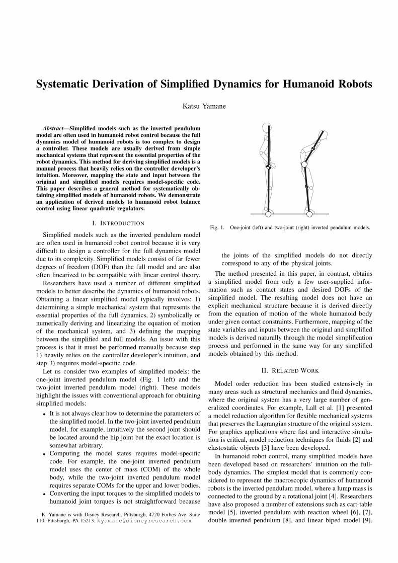
Let us consider two examples of simplified models: the

one-joint inverted pendulum model (Fig. 1 left) and the

two-joint inverted pendulum model (right). These models

highlight the issues with conventional approach for obtaining

simplified models:

• It is not always clear how to determine the parameters of

the simplified model. In the two-joint inverted pendulum

model, for example, intuitively the second joint should

be located around the hip joint but the exact location is

somewhat arbitrary.

• Computing the model states requires model-specific

code. For example, the one-joint inverted pendulum

model uses the center of mass (COM) of the whole

body, while the two-joint inverted pendulum model

requires separate COMs for the upper and lower bodies.

• Converting the input torques to the simplified models to

humanoid joint torques is not straightforward because

K. Yamane is with Disney Research, Pittsburgh, 4720 Forbes Ave. Suite110, Pittsburgh, PA 15213. [email protected]

Fig. 1. One-joint (left) and two-joint (right) inverted pendulum models.

the joints of the simplified models do not directly

correspond to any of the physical joints.

The method presented in this paper, in contrast, obtains

a simplified model from only a few user-supplied infor-

mation such as contact states and desired DOFs of the

simplified model. The resulting model does not have an

explicit mechanical structure because it is derived directly

from the equation of motion of the whole humanoid body

under given contact constraints. Furthermore, mapping of the

state variables and inputs between the original and simplified

models is derived naturally through the model simplification

process and performed in the same way for any simplified

models obtained by this method.

II. RELATED WORK

Model order reduction has been studied extensively in

many areas such as structural mechanics and fluid dynamics,

where the original system has a very large number of gen-

eralized coordinates. For example, Lall et al. [1] presented

a model reduction algorithm for flexible mechanical systems

that preserves the Lagrangian structure of the original system.

For graphics applications where fast and interactive simula-

tion is critical, model reduction techniques for fluids [2] and

elastostatic objects [3] have been developed.

In humanoid robot control, many simplified models have

been developed based on researchers’ intuition on the full-

body dynamics. The simplest model that is commonly con-

sidered to represent the macroscopic dynamics of humanoid

robots is the inverted pendulum model, where a lump mass is

connected to the ground by a rotational joint [4]. Researchers

have also proposed a number of extensions such as cart-table

model [5], inverted pendulum with reaction wheel [6], [7],

double inverted pendulum [8], and linear biped model [9].

Whether these models accurately represent the robot dy-

namics is not usually investigated in depth. An exception

can be found in [10] where the author derived the physical

relationships between a planar biped model and the Reaction

Mass Pendulum model [7].

Our model reduction method is similar to that of Hyland et

al. [11] where the reduced model is computed by minimizing

the difference between the outputs simulated by the original

and reduced models. They assume that the original dynamics

model is stable in order to make the error finite, which is

often not the case with free-standing humanoid robots. We

instead minimize the difference between the kinetic energies

to deal with this issue.

III. MODEL REDUCTION

A. Simplified Linear Model

The objective of this section is to approximate the dynam-

ics of a humanoid robot with n degrees of freedom (DOF),

possibly subject to contact constraints, by a k(≪ n)-DOF

linear system

Mq + Cq + Gq = u (1)

where q ∈ Rk is the generalized coordinate of the simplified

model, u ∈ Rk is the input force to the simplified model,

M ∈ Rk×k is a symmetric, positive-definite inertia matrix,

and C ∈ Rk×k and G ∈ Rk×k are constant matrices.

Because M is positive definite, we can rewrite Eq.(1) as

q = Φu− ΦGq − ΦCq (2)

where Φ = M−1

. We can then derive a state-space differ-

ential equation model

x = Ax+Bu (3)

by defining

x =

(

q

q

)

A =

(

0k×k 1k×k

−ΦG −ΦC

)

B =

(

0k×k

Φ

)

where 0∗ and 1∗ represent the zero and identity matrices of

the size indicated by the subscript.

This model is usually obtained by symbolically or numer-

ically evaluating and differentiating the Lagrangian equation

of motion of a simple mechanical model that represents the

essential properties of the full dynamics. In the following

subsections, we describe a more systematic method for

obtaining a simplified model (2).

B. Full Dynamics Model with Contact Constraints

We first review the original full-body dynamics of a

humanoid robot subject to contact constraints.

Consider a humanoid robot with n DOF, 6 of which

correspond to the translation and rotation of the base body

and therefore are not actuated. Also consider the case where

one or more links of the robot are in contact with the envi-

ronment, enforcing m independent constraints. The dynamics

of the humanoid robot is described by

M(θ)θ + c(θ, θ) + g(θ) = STτ + JTC(θ)fC (4)

where

θ ∈ Rn : generalized coordinates

τ ∈ Rn−6 : active joint torques

fC ∈ Rm : contact forces

M (θ) ∈ Rn×n : joint-space inertia matrix

c(θ, θ) ∈ Rn : centrifugal and Coriolis forces

g(θ) ∈ Rn : gravitational force

JC(θ) ∈ Rm×n : contact Jacobian matrix

and ST∈ Rn×(n−6) is the matrix that converts active joint

torques to generalized forces and typically has the form

ST =

(

06×(n−6)

1(n−6)×(n−6)

)

. (5)

The contact constraint is represented as

JC θ + JC θ = 0m. (6)

We can obtain the relationship between the generalized

acceleration θ and active joint torques τ by the following

procedure:

1) solve Eq.(4) for θ and plug the result into Eq.(6)

2) solve the resulting equation for fC

3) plug fC back into Eq.(4)

which results in

θ = Φ(θ)STτ + φ(θ, θ) (7)

where

Φ(θ) = M−1−M−1JT

C(JCM−1JT

C)−1JCM

−1

φ(θ, θ) = −M−1JTC(JCM

−1JTC)

−1JC θ −Φ(c + g).

Equation (7) describes the relationship between active joint

torques and joint accelerations (including the base body)

assuming that the contact constraints are satisfied. Note that

while M is positive definite, Φ is only positive semi-definite

due to the contact constraints, and therefore we cannot

compute Φ−1. This property corresponds to the fact that θ

that violates the contact constraints cannot be generated by

any generalized force.

C. Linearized Full Dynamics Model

Because our goal is to derive a simplified linear model,

we first linearize the original nonlinear model (7) around a

given nominal state (θT θT)T = (θT

0 0Tn )

T . If we define τ 0

as the joint torques required to maintain the nominal pose,

τ 0 satisfies

0n = Φ0STτ 0 + φ0. (8)

where Φ0 = Φ(θ0) and φ0 = φ(θ0,0n).

When the pose and velocity change by a small amount δθand δθ respectively, the equation of motion becomes

δθ = Φ(θ0 + δθ)STτ + φ(θ0 + δθ, δθ). (9)

Defining τ = τ 0 + δτ , using Eq.(8), and omitting second-

order terms of small changes, we obtain

δθ = Φ0ST δτ + (Φ′

τ + φ′

p)δθ + φ′

vδθ

= Φ0ST δτ + Γδθ +Λδθ (10)

where Φ′

τ = ∂(ΦSTτ 0)/∂θ, φ′

p = ∂φ/∂θ, and φ′

v =

∂φ/∂θ.

D. Model Reduction

We now describe the model reduction process consisting

of two steps: 1) compute Φ by singular value decomposition

(SVD) of Φ, and 2) obtain G and C by computing τ at

various poses around a nominal pose.

1) Computing Φ: Because Φ0 is symmetric and positive

semi-definite, its SVD results in

Φ0 = UΣUT (11)

where U ∈ Rn×n is an orthogonal matrix containing the

singular vectors and Σ ∈ Rn×n is a diagonal matrix whose

diagonal elements σi (i = 1, 2, . . . , n) are the singular values

of Φ0 and are sorted in the descending order (σ1 ≥ σ2 ≥

. . . ≥ σn ≥ 0).Suppose we approximate Φ0 by selecting k non-zero

diagonal elements of Σ and corresponding columns of U ,

such that

Φ0 ≈ Φ0 = UΣUT

(12)

with U ∈ Rn×k and Σ ∈ Rk×k. Choosing appropriate

singular values from Σ will be discussed later.

Plugging Eq.(12) into Eq.(10) yields

δθ = UΣUTST δτ + Γδθ +Λδθ. (13)

We then left-multiply UT

to the both sides of Eq.(13), which

results in

UTδθ = ΣU

TST δτ + U

TΓδθ + U

TΛδθ (14)

because UTU = 1k×k.

Let us define a mapping from the generalized coordinates

of the simplified model to those of the original model by

δθ = Uq. (15)

A possible inverse mapping is

q = UTδθ. (16)

We then consider the power that the inputs to the original

model produce:

δθTSTτ = qT U

TST δτ (17)

which indicates that we can match this power to that of the

simplified model by mapping the inputs by

u = UTST δτ (18)

Plugging them into Eq.(14), we obtain

q = Σu+ UTΓδθ + U

TΛδθ. (19)

Note that the right-hand side of this equation has the same

form as Eq.(2) with

M−1

= Φ = Σ (20)

G = −Σ−1

UTΓU (21)

C = −Σ−1

UTΛU (22)

because Σ is a diagonal matrix with positive elements.

2) Computing G and C: We employ a sampling-based

numerical method for computing these matrices.

We first obtain G by sampling a number of poses around

θ0 and computing the joint torques for realizing θ = 0n

and θ = 0n at each sample. Let us denote the difference

between θ0 and the i-th sample pose by ∆θi. Using an

inverse kinematics algorithm, we modify ∆θi to ∆θ′

i so

that the pose θ0 +∆θ′

i satisfies the contact constraints. We

then compute the joint torques τ i required to produce zero

accelerations.

Using the mapping equations (16)(18), we convert the

above quantities to those of the simplified model and plug

them into Eq.(1), obtaining

GUT∆θ′

i = UTSTτ i. (23)

By collecting ∆θ′

i and τ i from a number of samples and

solving a linear equation in the elements of G, we obtain G

that best fits the samples.

C can be computed by a similar process by sampling ∆θ

as well as ∆θ. Instead of zero accelerations, we compute the

accelerations that satisfy the kinematic constraints (6) and

compute the corresponding joint torques. Because Φ and G

are already known, we can form a linear equation in the

elements of C.

Once we obtain Σ, G, and C , we can derive the linear

state-space model (3).

3) Selecting the Singular Values: A standard method for

dimensionality reduction is to keep the larger singular values

of Σ and corresponding singular vectors of U . In our

case, however, this method does not preserve the essential

properties of the original dynamics as illustrated below.

The dynamics of a physical system is often characterized

by the kinetic energy. Because Φ0 is the inverse inertia

matrix of the constrained system and is singular, we first

define Φ0 as

Φ0 = UΣUT

(24)

where Σ is a diagonal matrix whose diagonal elements are

the nonzero singular values of Φ0, and U is the matrix com-

posed of the singular vectors corresponding to the nonzero

singular values. We can then define the inverse of Φ0 as

Φ−10 = UΣ

−1U

T(25)

which is essentially the inertia matrix of the constrained

system, because the robot cannot move in the directions of

the singular vectors of the zero singular values. The kinetic

energy is therefore

T =1

2θTΦ

−10 θ (26)

while the kinetic energy of the simplified model is

T =1

2qTMq

=1

2qT

Σ−1

q

=1

2δθ

TUΣ

−1U

Tδθ

=1

2θTΦ

−1

0 θ (27)

where we used Eqs.(20), (12), and (16).

In order to match T with T , we would like to make

Φ−1

0 ≈ Φ−10 which means that we should choose the largest

singular values of Φ−10 , or in other words, the smallest

nonzero singular values of Φ0.

More formally, the singular values of Φ0 are organized as

σ1 ≥ σ2 ≥ . . . ≥ σl > σl+1 = σl+2 = . . . = σn = 0 where lis the index of the last nonzero singular value. Following the

above discussion, we keep the smallest k nonzero singular

values (σl−k+1 to σl) for Σ and their corresponding singular

vectors for U .

E. Model Reduction Results

We show an example of model reduction using a humanoid

robot model with n = 38 DOF (32 rotational joints) and

flat contacts at both feet. Figure 2 visualizes the eight most

relevant singular vectors. In this case, Φ has six zero singular

values and therefore l = 32.

In Fig. 2, the black lines and spheres represent the link

segments and joints of the humanoid robot model. The

singular vector elements are represented by green and red

lines starting from corresponding joints. For each rotational

joint, a red line parallel to its axis is drawn with a length

proportional to the magnitude of the corresponding singular

vector element. If the element is negative, the line points the

opposite direction of the joint axis. For the base body, red

lines corresponding to the rotational degrees of freedom are

drawn in the same way, while the green lines represent the

elements corresponding to the linear degrees of freedom.

The left-most figure in Fig. 2 depicts the singular vector

corresponding to the smallest non-zero singular value (σl),

that is, the largest inertia. The singular vector shows that this

singular vector corresponds to leaning forward. Similarly,

the second to eighth smallest nonzero singular value roughly

correspond to the following motions:

1) σl−1: leaning left

2) σl−2: bending the upper body to the left

3) σl−3: twisting the body to the right

4) σl−4: bending the upper body forward

5) σl−5: swinging both arms inwards

6) σl−6: swinging both arms backwards

7) σl−7: swinging both arms to the right

While these singular vectors are computed automatically,

we can observe intuitive relationships with existing simplified

models. For example, if we only use the first singular value

(σl), the model would be similar to the single-inverted

pendulum in the sagittal plane, while the second singular

value (σl−1) would give the pendulum in the coronal plane.

The third (σl−2) and fifth (σl−4) singular values correspond

to the second joint of the two-joint inverted pendulum models

in the sagittal and coronal planes respectively. The sixth

singular value (σl−5) corresponds to changing the inertia

around the COM, which is explicitly modeled in the Reaction

Mass Pendulum model [7]. Finally, the seventh (σl−6) and

eighth (σl−7) singular values correspond to shifting the COM

without changing the contact point, which is modeled in the

cart-table model [5].

On the other hand, the twist motion (σl−3) is rarely

considered in simplified humanoid models but turns out

to be fairly important at least in terms of the associated

inertia. In the result section, we will show an example where

considering this mode appears to be critical in recovering a

balanced pose.

Another interesting observation is that the vertical COM

motion, often considered for controlling running and jump-

ing, does not appear among the most important modes. This

is probably because the knee joints in this particular nominal

pose are almost straight and therefore cannot easily generate

vertical COM motion. In fact, this mode appears as the

sixth mode when we compute the simplified model with bent

knees. This result implies that task-specific simplified model

may be obtained by simply using appropriate nominal pose.

IV. APPLICATION TO CONTROL

We demonstrate an application of simplified models de-

rived by our method to balance control of a humanoid robot.

Because one of the advantages of our method is that multiple

models can be generated and used with the same code, we

also demonstrate a scenario where multiple controllers are

used in sequence to generate complex motions.

A. Computing the Joint Torques

Recall the input mapping

u = UTST δτ (28)

where the mapping from original model to simplified model

is unique, but the reverse is not. We can take advantage of

this property to consider other factors to determine the joint

torques. This section shows an example of computing the

joint torques through numerical optimization.

A controller designed for the simplified model computes

a desired input u∗ to the simplified model. We also usually

want to consider the reference trajectories for the joints

because the controller for the simplified model does not con-

sider the individual joints. We can formulate an optimization

problem for computing the joint torque τ and the expected

contact forces fc with a cost function considering these two

terms.

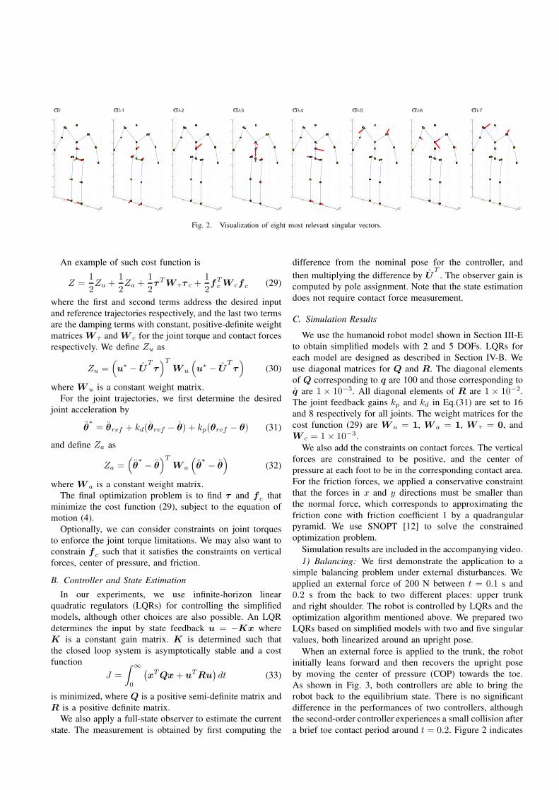
σl σl-1 σl-2 σl-3 σl-4 σl-5 σl-6 σl-7

Fig. 2. Visualization of eight most relevant singular vectors.

An example of such cost function is

Z =1

2Zu +

1

2Za +

1

2τTW ττ c +

1

2fTc W cfc (29)

where the first and second terms address the desired input

and reference trajectories respectively, and the last two terms

are the damping terms with constant, positive-definite weight

matrices W τ and W c for the joint torque and contact forces

respectively. We define Zu as

Zu =(

u∗− U

Tτ)T

W u

(

u∗− U

Tτ)

(30)

where W u is a constant weight matrix.

For the joint trajectories, we first determine the desired

joint acceleration by

θ∗

= θref + kd(θref − θ) + kp(θref − θ) (31)

and define Za as

Za =(

θ∗

− θ)T

W a

(

θ∗

− θ)

(32)

where W a is a constant weight matrix.

The final optimization problem is to find τ and fc that

minimize the cost function (29), subject to the equation of

motion (4).

Optionally, we can consider constraints on joint torques

to enforce the joint torque limitations. We may also want to

constrain fc such that it satisfies the constraints on vertical

forces, center of pressure, and friction.

B. Controller and State Estimation

In our experiments, we use infinite-horizon linear

quadratic regulators (LQRs) for controlling the simplified

models, although other choices are also possible. An LQR

determines the input by state feedback u = −Kx where

K is a constant gain matrix. K is determined such that

the closed loop system is asymptotically stable and a cost

function

J =

∫

∞

0

(

xTQx+ uTRu)

dt (33)

is minimized, where Q is a positive semi-definite matrix and

R is a positive definite matrix.

We also apply a full-state observer to estimate the current

state. The measurement is obtained by first computing the

difference from the nominal pose for the controller, and

then multiplying the difference by UT

. The observer gain is

computed by pole assignment. Note that the state estimation

does not require contact force measurement.

C. Simulation Results

We use the humanoid robot model shown in Section III-E

to obtain simplified models with 2 and 5 DOFs. LQRs for

each model are designed as described in Section IV-B. We

use diagonal matrices for Q and R. The diagonal elements

of Q corresponding to q are 100 and those corresponding to

q are 1 × 10−3. All diagonal elements of R are 1 × 10−2.

The joint feedback gains kp and kd in Eq.(31) are set to 16

and 8 respectively for all joints. The weight matrices for the

cost function (29) are W u = 1, W a = 1, W τ = 0, and

W c = 1× 10−3.

We also add the constraints on contact forces. The vertical

forces are constrained to be positive, and the center of

pressure at each foot to be in the corresponding contact area.

For the friction forces, we applied a conservative constraint

that the forces in x and y directions must be smaller than

the normal force, which corresponds to approximating the

friction cone with friction coefficient 1 by a quadrangular

pyramid. We use SNOPT [12] to solve the constrained

optimization problem.

Simulation results are included in the accompanying video.

1) Balancing: We first demonstrate the application to a

simple balancing problem under external disturbances. We

applied an external force of 200 N between t = 0.1 s and

0.2 s from the back to two different places: upper trunk

and right shoulder. The robot is controlled by LQRs and the

optimization algorithm mentioned above. We prepared two

LQRs based on simplified models with two and five singular

values, both linearized around an upright pose.

When an external force is applied to the trunk, the robot

initially leans forward and then recovers the upright pose

by moving the center of pressure (COP) towards the toe.

As shown in Fig. 3, both controllers are able to bring the

robot back to the equilibrium state. There is no significant

difference in the performances of two controllers, although

the second-order controller experiences a small collision after

a brief toe contact period around t = 0.2. Figure 2 indicates

0 0.5 1 1.5 2−0.25

−0.2

−0.15

−0.1

−0.05

0

0.05

q1

q2

time (s)

generalized coordinate value

0 0.5 1 1.5 2−0.25

−0.2

−0.15

−0.1

−0.05

0

0.05

0.1

q1

q2

q3

q4

q5

time (s)

generalized coordinate value

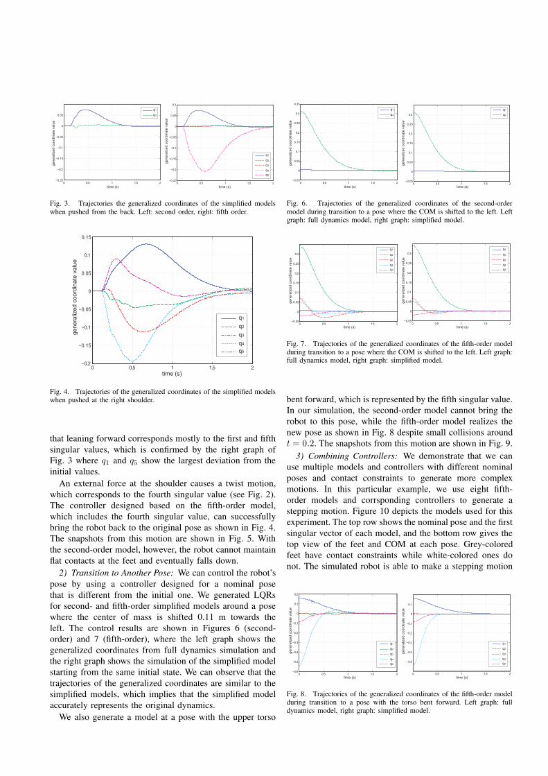
Fig. 3. Trajectories the generalized coordinates of the simplified modelswhen pushed from the back. Left: second order, right: fifth order.

0 0.5 1 1.5 2−0.2

−0.15

−0.1

−0.05

0

0.05

0.1

0.15

q1

q2

q3

q4

q5

time (s)

generalized coordinate value

Fig. 4. Trajectories of the generalized coordinates of the simplified modelswhen pushed at the right shoulder.

that leaning forward corresponds mostly to the first and fifth

singular values, which is confirmed by the right graph of

Fig. 3 where q1 and q5 show the largest deviation from the

initial values.

An external force at the shoulder causes a twist motion,

which corresponds to the fourth singular value (see Fig. 2).

The controller designed based on the fifth-order model,

which includes the fourth singular value, can successfully

bring the robot back to the original pose as shown in Fig. 4.

The snapshots from this motion are shown in Fig. 5. With

the second-order model, however, the robot cannot maintain

flat contacts at the feet and eventually falls down.

2) Transition to Another Pose: We can control the robot’s

pose by using a controller designed for a nominal pose

that is different from the initial one. We generated LQRs

for second- and fifth-order simplified models around a pose

where the center of mass is shifted 0.11 m towards the

left. The control results are shown in Figures 6 (second-

order) and 7 (fifth-order), where the left graph shows the

generalized coordinates from full dynamics simulation and

the right graph shows the simulation of the simplified model

starting from the same initial state. We can observe that the

trajectories of the generalized coordinates are similar to the

simplified models, which implies that the simplified model

accurately represents the original dynamics.

We also generate a model at a pose with the upper torso

0 0.5 1 1.5 2−0.05

0

0.05

0.1

0.15

0.2

0.25

0.3

0.35

q1

q2

time (s)

generalized coordinate value

0 0.5 1 1.5 2−0.05

0

0.05

0.1

0.15

0.2

0.25

0.3

q1

q2

time (s)

generalized coordinate value

Fig. 6. Trajectories of the generalized coordinates of the second-ordermodel during transition to a pose where the COM is shifted to the left. Leftgraph: full dynamics model, right graph: simplified model.

0 0.5 1 1.5 2−0.05

0

0.05

0.1

0.15

0.2

0.25

0.3

q1

q2

q3

q4

q5

time (s)

generalized coordinate value

0 0.5 1 1.5 2−0.05

0

0.05

0.1

0.15

0.2

0.25

0.3

q1

q2

q3

q4

q5

time (s)

generalized coordinate value

Fig. 7. Trajectories of the generalized coordinates of the fifth-order modelduring transition to a pose where the COM is shifted to the left. Left graph:full dynamics model, right graph: simplified model.

bent forward, which is represented by the fifth singular value.

In our simulation, the second-order model cannot bring the

robot to this pose, while the fifth-order model realizes the

new pose as shown in Fig. 8 despite small collisions around

t = 0.2. The snapshots from this motion are shown in Fig. 9.

3) Combining Controllers: We demonstrate that we can

use multiple models and controllers with different nominal

poses and contact constraints to generate more complex

motions. In this particular example, we use eight fifth-

order models and corrsponding controllers to generate a

stepping motion. Figure 10 depicts the models used for this

experiment. The top row shows the nominal pose and the first

singular vector of each model, and the bottom row gives the

top view of the feet and COM at each pose. Grey-colored

feet have contact constraints while white-colored ones do

not. The simulated robot is able to make a stepping motion

0 0.5 1 1.5 2−0.6

−0.5

−0.4

−0.3

−0.2

−0.1

0

0.1

0.2

q1

q2

q3

q4

q5

time (s)

generalized coordinate value

0 0.5 1 1.5 2

−0.5

−0.4

−0.3

−0.2

−0.1

0

0.1

q1

q2

q3

q4

q5

time (s)

generalized coordinate value

Fig. 8. Trajectories of the generalized coordinates of the fifth-order modelduring transition to a pose with the torso bent forward. Left graph: fulldynamics model, right graph: simplified model.

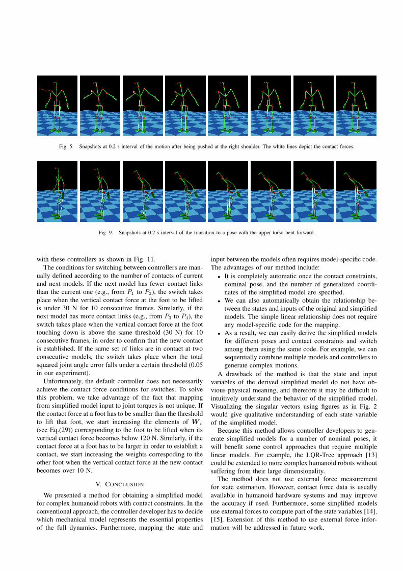
Fig. 5. Snapshots at 0.2 s interval of the motion after being pushed at the right shoulder. The white lines depict the contact forces.

Fig. 9. Snapshots at 0.2 s interval of the transition to a pose with the upper torso bent forward.

with these controllers as shown in Fig. 11.

The conditions for switching between controllers are man-

ually defined according to the number of contacts of current

and next models. If the next model has fewer contact links

than the current one (e.g., from P1 to P2), the switch takes

place when the vertical contact force at the foot to be lifted

is under 30 N for 10 consecutive frames. Similarly, if the

next model has more contact links (e.g., from P3 to P4), the

switch takes place when the vertical contact force at the foot

touching down is above the same threshold (30 N) for 10

consecutive frames, in order to confirm that the new contact

is established. If the same set of links are in contact at two

consecutive models, the switch takes place when the total

squared joint angle error falls under a certain threshold (0.05

in our experiment).

Unfortunately, the default controller does not necessarily

achieve the contact force conditions for switches. To solve

this problem, we take advantage of the fact that mapping

from simplified model input to joint torques is not unique. If

the contact force at a foot has to be smaller than the threshold

to lift that foot, we start increasing the elements of W c

(see Eq.(29)) corresponding to the foot to be lifted when its

vertical contact force becomes below 120 N. Similarly, if the

contact force at a foot has to be larger in order to establish a

contact, we start increasing the weights correspoding to the

other foot when the vertical contact force at the new contact

becomes over 10 N.

V. CONCLUSION

We presented a method for obtaining a simplified model

for complex humanoid robots with contact constraints. In the

conventional approach, the controller developer has to decide

which mechanical model represents the essential properties

of the full dynamics. Furthermore, mapping the state and

input between the models often requires model-specific code.

The advantages of our method include:

• It is completely automatic once the contact constraints,

nominal pose, and the number of generalized coordi-

nates of the simplified model are specified.

• We can also automatically obtain the relationship be-

tween the states and inputs of the original and simplified

models. The simple linear relationship does not require

any model-specific code for the mapping.

• As a result, we can easily derive the simplified models

for different poses and contact constraints and switch

among them using the same code. For example, we can

sequentially combine multiple models and controllers to

generate complex motions.

A drawback of the method is that the state and input

variables of the derived simplified model do not have ob-

vious physical meaning, and therefore it may be difficult to

intuitively understand the behavior of the simplified model.

Visualizing the singular vectors using figures as in Fig. 2

would give qualitative understanding of each state variable

of the simplified model.

Because this method allows controller developers to gen-

erate simplified models for a number of nominal poses, it

will benefit some control approaches that require multiple

linear models. For example, the LQR-Tree approach [13]

could be extended to more complex humanoid robots without

suffering from their large dimensionality.

The method does not use external force measurement

for state estimation. However, contact force data is usually

available in humanoid hardware systems and may improve

the accuracy if used. Furthermore, some simplified models

use external forces to compute part of the state variables [14],

[15]. Extension of this method to use external force infor-

mation will be addressed in future work.

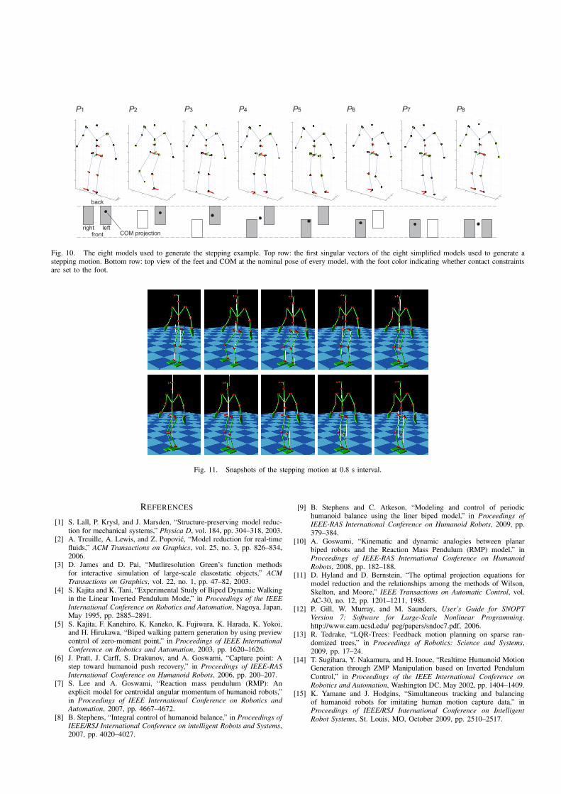
P1 P2 P3 P4 P5 P6 P7 P8

leftrightCOM projectionfront

back

Fig. 10. The eight models used to generate the stepping example. Top row: the first singular vectors of the eight simplified models used to generate astepping motion. Bottom row: top view of the feet and COM at the nominal pose of every model, with the foot color indicating whether contact constraintsare set to the foot.

Fig. 11. Snapshots of the stepping motion at 0.8 s interval.

REFERENCES

[1] S. Lall, P. Krysl, and J. Marsden, “Structure-preserving model reduc-tion for mechanical systems,” Physica D, vol. 184, pp. 304–318, 2003.

[2] A. Treuille, A. Lewis, and Z. Popovic, “Model reduction for real-timefluids,” ACM Transactions on Graphics, vol. 25, no. 3, pp. 826–834,2006.

[3] D. James and D. Pai, “Mutliresolution Green’s function methodsfor interactive simulation of large-scale elasostatic objects,” ACM

Transactions on Graphics, vol. 22, no. 1, pp. 47–82, 2003.[4] S. Kajita and K. Tani, “Experimental Study of Biped Dynamic Walking

in the Linear Inverted Pendulum Mode,” in Proceedings of the IEEE

International Conference on Robotics and Automation, Nagoya, Japan,May 1995, pp. 2885–2891.

[5] S. Kajita, F. Kanehiro, K. Kaneko, K. Fujiwara, K. Harada, K. Yokoi,and H. Hirukawa, “Biped walking pattern generation by using previewcontrol of zero-moment point,” in Proceedings of IEEE International

Conference on Robotics and Automation, 2003, pp. 1620–1626.[6] J. Pratt, J. Carff, S. Drakunov, and A. Goswami, “Capture point: A

step toward humanoid push recovery,” in Proceedings of IEEE-RAS

International Conference on Humanoid Robots, 2006, pp. 200–207.[7] S. Lee and A. Goswami, “Reaction mass pendulum (RMP): An

explicit model for centroidal angular momentum of humanoid robots,”in Proceedings of IEEE International Conference on Robotics andAutomation, 2007, pp. 4667–4672.

[8] B. Stephens, “Integral control of humanoid balance,” in Proceedings ofIEEE/RSJ International Conference on intelligent Robots and Systems,2007, pp. 4020–4027.

[9] B. Stephens and C. Atkeson, “Modeling and control of periodichumanoid balance using the liner biped model,” in Proceedings of

IEEE-RAS International Conference on Humanoid Robots, 2009, pp.379–384.

[10] A. Goswami, “Kinematic and dynamic analogies between planarbiped robots and the Reaction Mass Pendulum (RMP) model,” inProceedings of IEEE-RAS International Conference on Humanoid

Robots, 2008, pp. 182–188.[11] D. Hyland and D. Bernstein, “The optimal projection equations for

model reduction and the relationships among the methods of Wilson,Skelton, and Moore,” IEEE Transactions on Automatic Control, vol.AC-30, no. 12, pp. 1201–1211, 1985.

[12] P. Gill, W. Murray, and M. Saunders, User’s Guide for SNOPT

Version 7: Software for Large-Scale Nonlinear Programming.http://www.cam.ucsd.edu/ peg/papers/sndoc7.pdf, 2006.

[13] R. Tedrake, “LQR-Trees: Feedback motion planning on sparse ran-domized trees,” in Proceedings of Robotics: Science and Systems,2009, pp. 17–24.

[14] T. Sugihara, Y. Nakamura, and H. Inoue, “Realtime Humanoid MotionGeneration through ZMP Manipulation based on Inverted PendulumControl,” in Proceedings of the IEEE International Conference on

Robotics and Automation, Washington DC, May 2002, pp. 1404–1409.[15] K. Yamane and J. Hodgins, “Simultaneous tracking and balancing

of humanoid robots for imitating human motion capture data,” inProceedings of IEEE/RSJ International Conference on Intelligent

Robot Systems, St. Louis, MO, October 2009, pp. 2510–2517.