System identification of nonlinear autoregressive models in monitoring dengue infection

SYSTEM IDENTIFICATION OF NONLINEAR

AUTOREGRESSIVE MODELS IN MONITORING DENGUE

INFECTION

#H. Abdul Rahim1, F. Ibrahim2 and M. N. Taib3

1Department of Control and Instrumentation Engineering,Faculty of Electrical

Engineering,Universiti Teknologi Malaysia,81310 UTM Skudai, Johor, Malaysia.

2Department of Biomedical Engineering,Faculty of Engineering,University of Malaya,

50603 Kuala Lumpur, Malaysia.

3Faculty of Electrical Engineering,Universiti Teknologi Mara,

40450 Shah Alam, Selangor, Malaysia.

#Emails: [email protected]

Abstract-This paper proposes system identification on application of nonlinear AR (NAR)

based on Artificial Neural Network (ANN) for monitor of dengue infections. In building the

model, three selection criteria, i.e. the final prediction error (FPE), Akaike’s Information

Criteria (AIC), and Lipschitz number were used. Each of the models is divided into two

approaches, which are unregularized approach and regularized approach. The findings

indicate that NARMAX model with regularized approach yields better accuracy by 80.60%.

The best parameters’ settings for this thesis can be found using the Lipschitz number criterion

for the model order selection with artificial neural network structure of 4 trained using the

Levenberg Marquardt algorithm.

Index terms: dengue fever, NAR model, AIC, Lipschitz, FPE, ROC and AUC.

783

INTERNATIONAL JOURNAL ON SMART SENSING AND INTELLIGENT SYSTEMS, VOL. 3, NO. 4, DECEMBER 2010

1. INTRODUCTION

Dengue fever (DF) ranks highly among the newly emerging infectious diseases in public

health significance. Hence it is considered to be the most important of the arthropod-

borne viral diseases. In Malaysia, the disease is endemic but major outbreaks seem to

occur at least once in every four years [2]. Dengue fever was first reported in Malaysia

after an epidemic in Penang in 1902 [3, 4]. Since the early 1970s, the World Health

Organization (WHO) has been actively involved in developing and promoting strategies

for treatment and control of dengue. In 1997, WHO published a second guide to the

diagnosis, treatment and control of dengue haemorrhagic fever [1]. Dengue were

reported throughout the year and started to increase from 1997 to 1998. In 1998, 27,373

dengue cases with 58 deaths were reported as compared to 19,544 cases with 50 deaths in

1997. This has shown an increase of 7,829 cases or 40.1% over the number of cases in

1997 [5]. Therefore, accurate classification of dengue infection a very useful tool for

doctors in diagnosing diseases early.

Fatimah et. al. [6] describe a noninvasive prediction system for predicting the day of

defervescence of fever in dengue patients using ANN. The developed system bases its

prediction solely on clinical symptoms and signs and the results show that around 90%

prediction accuracy.

This paper describes a noninvasive classification system for dengue infections using

NAR models. The rest of the paper is structured as follows: In Section II nonlinear

autoregressive (NAR) model is presented. Methods are provided in Section III. In

Section IV shows the results. Finally, concluding remarks and discussions are presented

in Section V.

II. NONLINEAR AUTOREGRESSIVE MODEL

The NAR model consists of an autoregressive which is represented as past output data

and the nonlinear function was selected as hyperbolic tangent.

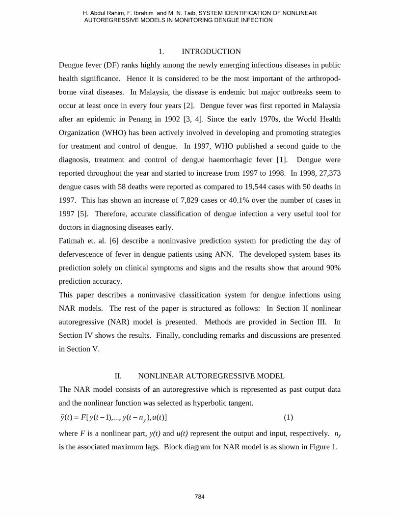
)](),(),...,1([)(ˆ tuntytyFty y−−= (1)

where F is a nonlinear part, y(t) and u(t) represent the output and input, respectively. ny

is the associated maximum lags. Block diagram for NAR model is as shown in Figure 1.

784

H. Abdul Rahim, F. Ibrahim and M. N. Taib, SYSTEM IDENTIFICATION OF NONLINEAR AUTOREGRESSIVE MODELS IN MONITORING DENGUE INFECTION

Figure 1: NAR Model

a. Model Order Selection

Model order selection is dependent upon the quality of the model since the model order is

varied and the cost function is monitored. A useful measure to aid this procedure is to

measure the significance of each additional model. Assessing the significance of each

model is not only necessary for model order selection but also for further analysis of the

estimated model and can aid the design and analysis of medical applications.

b. Model Estimation

The third step is model estimation, which involves determining the numerical values of

the structural parameters, which minimise the error between the system to be identified,

and its model.

c. Regularization

If the network has been trained to a very small value of criterion, the model needs not be

particularly good. A good performance on the training set does not automatically imply

that the model generalizes well to new inputs. In particular, it was shown that if the

model structure was too large (contained many weights) it led to overfitting [15], that is,

the noise in the training set was also modelled. The average generalization error was

introduced as a quantity assessing a given model structure. One way of controlling the

average generalization error was to extend the criterion with a term called regularization

by simple weight decay [15]. The weight decay reduced the variance error at the expense

of a higher bias error.

)(ˆ ty

u (t)

y (t-ny)

y (t-1)

F

785


d. Model Validation

Receiver operating characteristic (ROC) curves are commonly used in medicine and

healthcare [18], where they are used to quantify the accuracy of diagnostic tests [19, 20].

The performance of an “expert” human or machine, can be represented objectively by

ROC curves [21]. Such curves show, for example, the trade-off between a diagnostic test

correctly identifying diseased patients as diseased, rather than healthy, versus correctly

identifying healthy patients as healthy, rather than diseased. Terms commonly used in

ROC curves are sensitivity, specificity and diagnostic accuracy, to show the accuracy of

the designed system.

i. Receiver Operating Characteristic (ROC) Curves

ROC curves display the relationship between sensitivity (true positive rate) and 1-

specificity (false positive rate) across all possible threshold values that define the

positivity of a disease. They show the full picture trade-off between true positive rate and

false positive rate at different levels of positivity.

The ANN must be trained before the ROC curve can be generated. The resulting network

is referred to as a “basic trained network”. This initial instance of the ANN provides one

operating point. The result is a set of instances of the network chosen to represent a point

on the ROC curve. The goodness of this set of network instances are then evaluated

using separate test data.

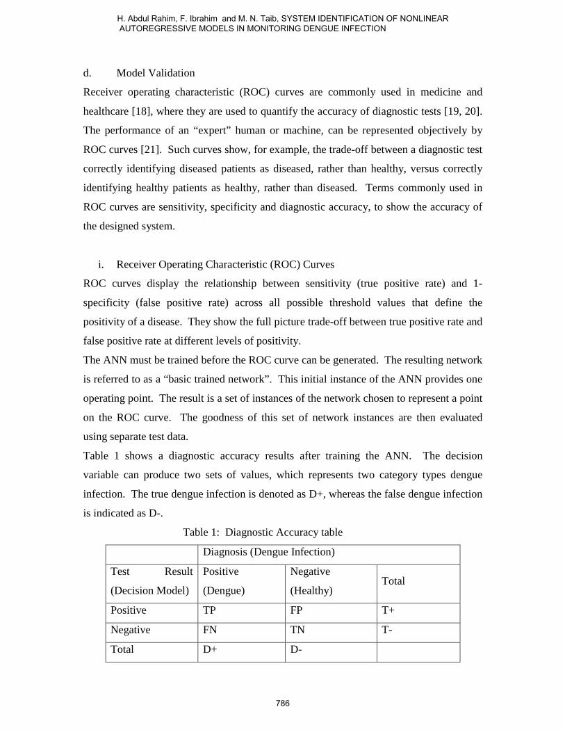
Table 1 shows a diagnostic accuracy results after training the ANN. The decision

variable can produce two sets of values, which represents two category types dengue

infection. The true dengue infection is denoted as D+, whereas the false dengue infection

is indicated as D-.

Table 1: Diagnostic Accuracy table

Diagnosis (Dengue Infection)

Test Result

(Decision Model)

Positive

(Dengue)

Negative

(Healthy) Total

Positive TP FP T+

Negative FN TN T-

Total D+ D-

786


In general, four possible decisions and two types of errors are made when comparing a

test result with a diagnosis, as shown in Table 1. If both diagnosis and test are positive, it

is called a true positive (TP). The probability of the TP to occur is estimated by counting

the true positives in the sample and dividing by the sample size. If the diagnosis is

positive and the test is negative it is called a false negative (FN). False positive (FP) and

true negative (TN) are defined similarly. The two sets of values produced in the

threshold are the total positive and negative indicated as T+ and T-.

Sensitivity and specificity are the basic measures of the accuracy of the diagnostic test.

They describe the abilities of the test to enable one to correctly diagnose disease when the

disease is actually present and to correctly rule out disease when it is truly absent.

The accuracy of a test is measured by comparing the results of the test to the true disease

status of the patient. Sensitivity and specificity depend on the threshold (also known as

‘operating point’ or ‘cut point’) used to define positive and negative test results. As the

threshold level decreases, the sensitivity increases while the specificity decreases, and

vice versa.

Sensitivity is the ratio or percentage of a probability that a test result will be positive

when the diagnosis is present, also known as true positive rate (TPR), defined as:

+=

DTPTPRySensitivit : (2)

Specificity is the ratio or percentage of a probability that a test result will be negative

when the disease is not present and also known as true negative rate (TNR), defined as:

−=

DTNTNRySpecificit : (3)

III. METHODOLOGY

a. Data Collection

The data were obtained from the previous work [22]. For the first group, the severity of

the DHF is classified into grade I to IV, according to WHO recommendation [23]. Acute

dengue infection was confirmed subsequently by the use of ELISA to detect elevated

dengue specific IgM (primary infection) and IgG (secondary infection) [24]. Patient

serum samples were tested for hemoglobin determination using an automated counter

787


(Coulter STKS machine). The second group is the control group for healthy female and

male subjects.

The second group of patients (control subjects) who do not have past medical history of

dengue were recruited and studied using the same guidelines as in the BIA subject

preparation used for the first group [22]. The BIA safety measurements procedure and

other safety precautions were made known to the subjects and their informed consent was

obtained from each subject prior to the BIA measurement.

For the control subject, the weight was taken once. However for subjects with dengue

infection, the weight was measured daily until upon discharged.

b. Clinical Experiments

One of the clinical methods in making dengue diagnosis is to establish the clinical

history-taking, physical examination and investigation. Each patient undergoes detailed

history taking, physical examinations and blood investigations following their admission.

Clinical evaluations and haematological investigations are conducted continuously until

they are discharged.

The patients were also admitted at different stages of their illness, thus it is important to

have the results of clinical signs and symptoms, blood investigations, and other analyses

dated with a consistent and proper reference point [22]. Nevertheless, thorough

documentation of symptoms and blood investigations do not offer definitive advantage in

the management and monitoring of dengue cases. A more useful measure is to develop a

complete day-to-day profile of clinical manifestations and blood investigations made

according to a proper reference point based on the ‘Fever day’ definition [22]. This is to

ensure that the data used in the analysis will refer to a common reference point,

regardless of how many days of fever the patient has experienced

The Hb status of control subjects cannot be determined at a low frequency of 50 kHz,

since the membranes of blood cells will act as insulators. In DHF patients however,

pathophysiological changes caused by the dengue infection lead to a plasma leakage. And

this in turn causes low thrombocytopenia and coagulopathy [23]. It is therefore possible

to estimate the Hb volume indirectly using the BIA technique.

788


c. BIA Experiments

The bioelectrical impedance experiments are conducted using the bioimpedance analyzer.

It is important to note that there is no historical or clinical evidence that bioimpedance

testing is unsafe, even for pregnant women or persons with pre-existing heart conditions.

During the years 2001 and 2002, two hundred and ten adult patients aged twelve years

old and above, with serological confirmation (WHO 1997) of acute dengue infection,

admitted in HUKM, Malaysia were prospectively studied. At present, the knowledge

acquisition to present pattern to classify the dengue infections is limited to the clinical

symptoms and signs. Thus, only clinical symptoms were used as the input data for

classify the dengue infections.

A total of one hundred and forty two volunteers with no past medical history were

recruited and studied as the control subjects. For the control subject the weight was taken

once, however for subjects with dengue infection the weight was measured daily until

upon discharged.

The statistical analysis was performed using SPSS statistical package version 10.01 for

Window 1998. Simple linear regression was used in the preliminary analysis for testing

the significance of the variables. These variables were then included in the multivariate

analysis. Multiple linear regression was used to analyse the control effects of the patient

demographic and symptom variables and BIA parameters on Hb. The model was

constructed in three steps as follows:

a. When correlation exits between variables, one or more variables were excluded

for the multivariate analysis.

b. The demographic variables were first included in the model. Once the

demographic predictors were identified, add in the BIA parameters and find,

which of these parameters were important predictors.

c. The last step was to include symptom and find out whether with the addition of

this predictor will make further significant contribution or not.

The last step was to include symptom and find out whether with the addition of this

predictor will make further significant contribution or not.

Only five variables are highly significant which gender, weight, reactance (Xc), vomiting

and day of fever [22, 25-27].

789


These predictors will be the inputs for linear and nonlinear system identification based on

ANN. All the inputs data for these models were normalized from ‘0’ to ‘1’. Only for

linear and nonlinear system identification based on ANN the output data were categorize

into 2 parts, for classifying the dengue infections disease which is 0 for no dengue

infection, while 1 for dengue infections.

Then, the input data were divided randomly, between 2 sets: a training set and a testing

set. These five input variables were fed into the FFNN and trained using LM algorithm.

During this process, the NAR application was optimized via four steps where each of

these steps was implemented to find optimum value for the model order, the number of

hidden layers, maximum iterations, and lastly the number of parameters regularization.

At each experiment, the respective parameter to be optimized was varied while the other

three were fixed. Selection of the optimum parameter value for each step was based on

the performance evaluation of the model through the final prediction error (FPE) analysis

as well as the diagnostic accuracy (DA). For simplicity, threshold for the output logic

levels was fixed to 0.5 for each models used in this work. At the next stage, the most

appropriate threshold level would be decided by analyzing the minimum Euclidean

Distance (ED) values from the receiver operating characteristic (ROC) plot.

Finally, the area under the ROC curve was applied to measure the accuracy of dengue

hemoglobin status in the diagnostic test.

d. Experiment for NAR Model

These experiments were designed to give better accuracy than the previous experiments

(linear model). These experiments processes (data preprocessing, model design, model

estimation and model validation) are described in next section.

790


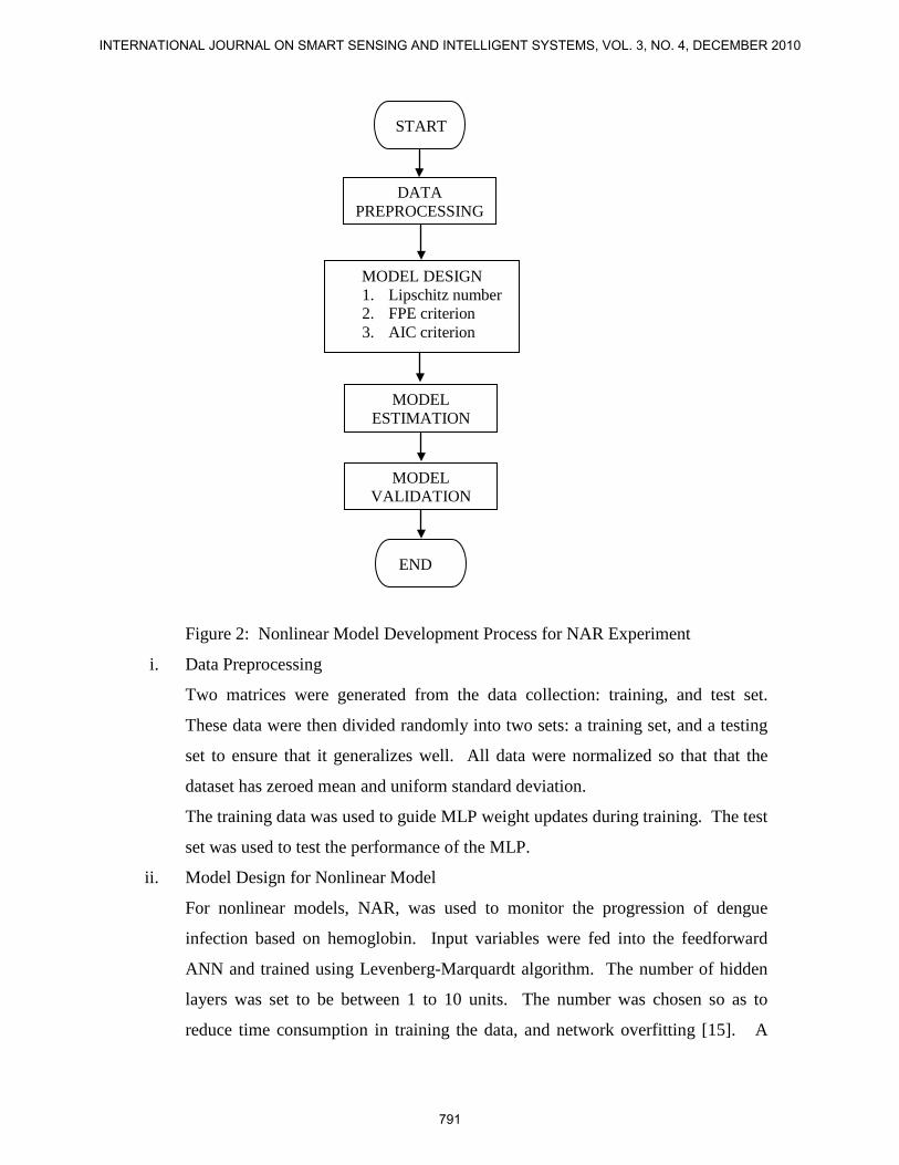
Figure 2: Nonlinear Model Development Process for NAR Experiment

i. Data Preprocessing

Two matrices were generated from the data collection: training, and test set.

These data were then divided randomly into two sets: a training set, and a testing

set to ensure that it generalizes well. All data were normalized so that that the

dataset has zeroed mean and uniform standard deviation.

The training data was used to guide MLP weight updates during training. The test

set was used to test the performance of the MLP.

ii. Model Design for Nonlinear Model

For nonlinear models, NAR, was used to monitor the progression of dengue

infection based on hemoglobin. Input variables were fed into the feedforward

ANN and trained using Levenberg-Marquardt algorithm. The number of hidden

layers was set to be between 1 to 10 units. The number was chosen so as to

reduce time consumption in training the data, and network overfitting [15]. A

DATA PREPROCESSING

MODEL DESIGN 1. Lipschitz number 2. FPE criterion 3. AIC criterion

MODEL ESTIMATION

END

START

MODEL VALIDATION

791


transfer function for neurons in the hidden layers is hyperbolic tangent sigmoid

and the single neuron in the output layer has a linear transfer function.

There were two approaches considered in this study, unregularized and

regularized approach. Unregularized approach is the normal method used for

training the networks, which is associated with Equation 3.42 for FPE. For the

regularized approach, it was shown that one way of controlling the average

generalization error was to extend the criterion with a term called regularization

by simple weight decay. The weight decay reduced the variance error at the

expense of a higher bias error. Nørgaard [15] showed that the value was obtained

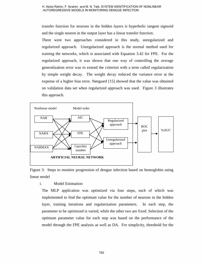
on validation data set when regularized approach was used. Figure 3 illustrates

this approach.

Figure 3: Steps to monitor progression of dengue infection based on hemoglobin using

linear model

i. Model Estimation

The MLP application was optimized via four steps, each of which was

implemented to find the optimum value for the number of neurons in the hidden

layer, training iterations and regularization parameters. In each step, the

parameter to be optimized is varied, while the other two are fixed. Selection of the

optimum parameter value for each step was based on the performance of the

model through the FPE analysis as well as DA. For simplicity, threshold for the

NAR

NARX

NARMAX

AIC

FPE

Lipschitz number

Nonlinear model Model order

Regularized approach

Unregularized approach

ROC plot

%AUC

ARTIFICIAL NEURAL NETWORK

792


output logic levels was fixed to 0.5 for each model used in this initial work. The

best model for the experiment was then selected for the final application.

ii. Validation of Nonlinear Models

In this stage, the most appropriate threshold level was decided by analyzing the

minimum ED values from the ROC plot. Finally the AUC was applied to

measure the accuracy of dengue hemoglobin status in diagnostic test.

IV. RESULTS

a. Dengue Data

During the year 2001 to 2002, two hundred and ten adult patients aged 12 to 83 years old,

suspected of DF and DHF admitted to the Universiti Kebangsaan Malaysia Hospital

(HUKM), were monitored. The dengue infection was also confirmed serologically by

detection of IgM antibody using the ELISA method. For all the 210 dengue patients

studied, 119 (56.7%) were male and 91 (43.3%) were females.

The sample size of the female was more than the male for DF by 4 patients. However,

for DHF I the males exceeded the females by 11; the males increased by 22 compared to

females in DHF II and there was only one female DSS patient. In the age distribution, the

majority were mainly in the 15-24 years group age (35.71%), followed by the 25-34 years

group age (25.24%). Those aged between 35-44 years constituted 20% for all cases. This

indicates that the majority of the patients were teenagers and young adults, whom were

more likely to be involved in outdoor activities and thus more likely to be exposed to the

danger of dengue infection.

b. Bioelectrical Impedance Analysis

In the analysis of bioelectrical tissue conductivity (BETC) parameters for the healthy

subjects, it was found that body capacitance (BC) and phase angle (α) were lower in the

female subjects compared to their male counterparts (Table 5.2). On the other hand,

resistor (R) and reactance (Xc) were higher in females than in males. A similar trend for

the BETC parameters was also observed in dengue patients, where a higher α and BC

values were found in males, and a higher R and Xc values were found in females. For

example, on ‘Fever day 0’, the mean α for male was 6.69±0.91° and female was

793


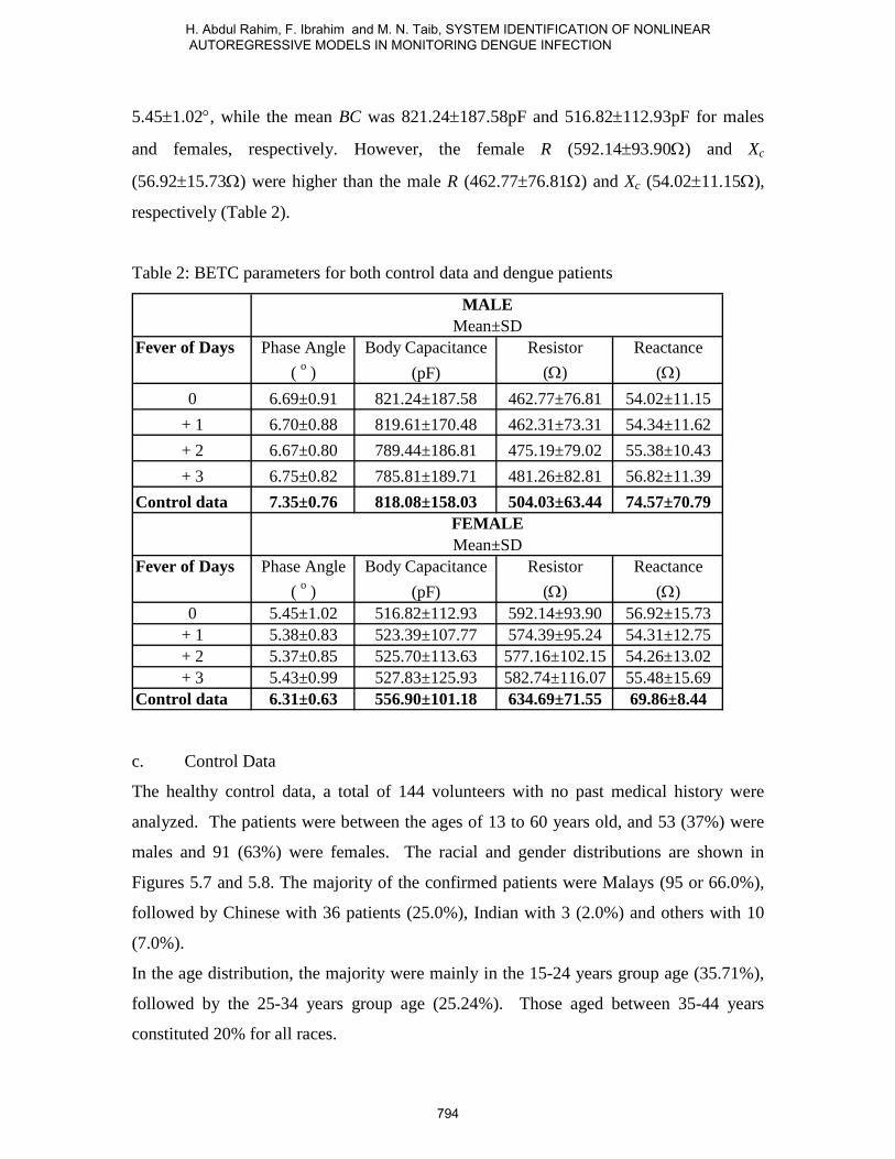
5.45±1.02°, while the mean BC was 821.24±187.58pF and 516.82±112.93pF for males

and females, respectively. However, the female R (592.14±93.90Ω) and Xc

(56.92±15.73Ω) were higher than the male R (462.77±76.81Ω) and Xc (54.02±11.15Ω),

respectively (Table 2).

Table 2: BETC parameters for both control data and dengue patients

Fever of Days Phase Angle Body Capacitance Resistor Reactance( o ) (pF) (Ω) (Ω)

0 6.69±0.91 821.24±187.58 462.77±76.81 54.02±11.15+ 1 6.70±0.88 819.61±170.48 462.31±73.31 54.34±11.62+ 2 6.67±0.80 789.44±186.81 475.19±79.02 55.38±10.43+ 3 6.75±0.82 785.81±189.71 481.26±82.81 56.82±11.39

Control data 7.35±0.76 818.08±158.03 504.03±63.44 74.57±70.79

Fever of Days Phase Angle Body Capacitance Resistor Reactance( o ) (pF) (Ω) (Ω)

0 5.45±1.02 516.82±112.93 592.14±93.90 56.92±15.73+ 1 5.38±0.83 523.39±107.77 574.39±95.24 54.31±12.75+ 2 5.37±0.85 525.70±113.63 577.16±102.15 54.26±13.02+ 3 5.43±0.99 527.83±125.93 582.74±116.07 55.48±15.69

Control data 6.31±0.63 556.90±101.18 634.69±71.55 69.86±8.44

FEMALEMean±SD

MALEMean±SD

c. Control Data

The healthy control data, a total of 144 volunteers with no past medical history were

analyzed. The patients were between the ages of 13 to 60 years old, and 53 (37%) were

males and 91 (63%) were females. The racial and gender distributions are shown in

Figures 5.7 and 5.8. The majority of the confirmed patients were Malays (95 or 66.0%),

followed by Chinese with 36 patients (25.0%), Indian with 3 (2.0%) and others with 10

(7.0%).

In the age distribution, the majority were mainly in the 15-24 years group age (35.71%),

followed by the 25-34 years group age (25.24%). Those aged between 35-44 years

constituted 20% for all races.

794


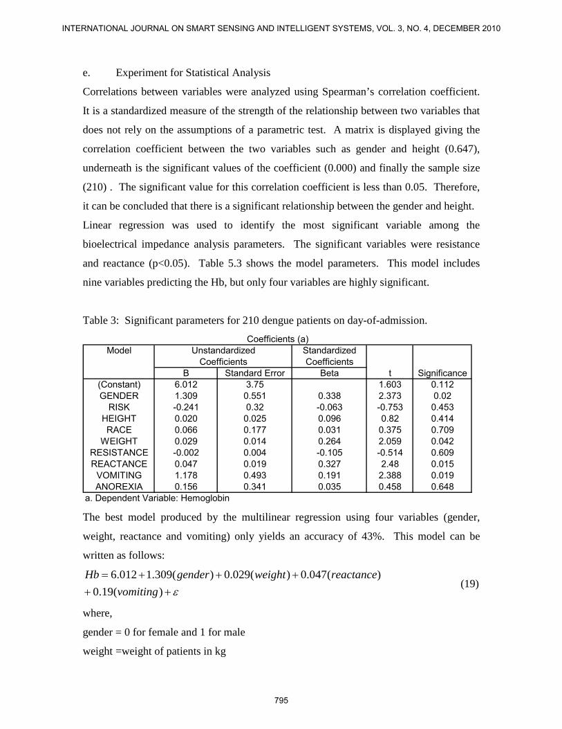
e. Experiment for Statistical Analysis

Correlations between variables were analyzed using Spearman’s correlation coefficient.

It is a standardized measure of the strength of the relationship between two variables that

does not rely on the assumptions of a parametric test. A matrix is displayed giving the

correlation coefficient between the two variables such as gender and height (0.647),

underneath is the significant values of the coefficient (0.000) and finally the sample size

(210) . The significant value for this correlation coefficient is less than 0.05. Therefore,

it can be concluded that there is a significant relationship between the gender and height.

Linear regression was used to identify the most significant variable among the

bioelectrical impedance analysis parameters. The significant variables were resistance

and reactance (p<0.05). Table 5.3 shows the model parameters. This model includes

nine variables predicting the Hb, but only four variables are highly significant.

Table 3: Significant parameters for 210 dengue patients on day-of-admission.

Model StandardizedCoefficients

B Standard Error Beta t Significance(Constant) 6.012 3.75 1.603 0.112GENDER 1.309 0.551 0.338 2.373 0.02

RISK -0.241 0.32 -0.063 -0.753 0.453HEIGHT 0.020 0.025 0.096 0.82 0.414RACE 0.066 0.177 0.031 0.375 0.709

WEIGHT 0.029 0.014 0.264 2.059 0.042RESISTANCE -0.002 0.004 -0.105 -0.514 0.609REACTANCE 0.047 0.019 0.327 2.48 0.015

VOMITING 1.178 0.493 0.191 2.388 0.019ANOREXIA 0.156 0.341 0.035 0.458 0.648

a. Dependent Variable: Hemoglobin

UnstandardizedCoefficients

Coefficients (a)

The best model produced by the multilinear regression using four variables (gender,

weight, reactance and vomiting) only yields an accuracy of 43%. This model can be

written as follows:

ε+++++=

)(19.0)(047.0)(029.0)(309.1012.6

vomitingreactanceweightgenderHb

(19)

where,

gender = 0 for female and 1 for male

weight =weight of patients in kg

795


react. = reactance of patients in ohm

vomiting = 1 for sign of vomit and 0 for no sign of vomit,

ε = error term

f. AR Experiment

Three types of input variables, which consisted of a list of dengue clinical symptoms,

physiological and BIA parameters, were used in the AR Experiments. These input

variables were analysed and evaluated using SPSS based on the hemoglobin

concentration.

g. Data Preprocessing

210 patients were monitored over a period of 4 succeeding days, depending on their

severity and duration of stay in the hospital. The patients’ symptoms, BIA parameters and

physiological data were monitored daily to form a unique set of samples, and producing a

total of 781 samples. All data were normalized from ‘0’ to ‘1’. These data were then

divided randomly into two sets: a training set consisting of 527 samples, and a testing set

of 254 samples. Each case was arranged as column vectors in the datasets.

The results show that there were only one symptom (vomiting), two physiological data

(gender and weight) and one BIA parameter (reactance) which were significant based on

Experiment for SPSS. These predictors were subsequently used as inputs for Experiment

for NAR. ‘Fever day 0’ to ‘Fever day +3’ were important references for the

physiological changes in the clinical symptoms. All of these parameters were employed

as the inputs for the system identification experiments.

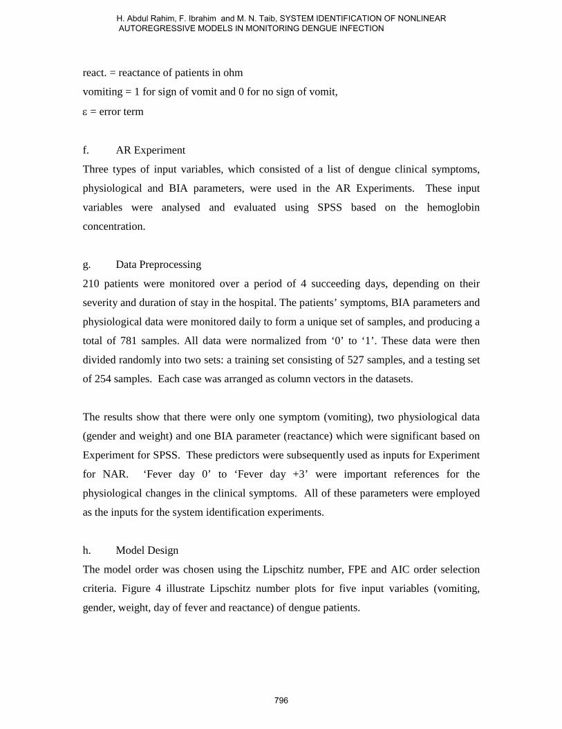
h. Model Design

The model order was chosen using the Lipschitz number, FPE and AIC order selection

criteria. Figure 4 illustrate Lipschitz number plots for five input variables (vomiting,

gender, weight, day of fever and reactance) of dengue patients.

796


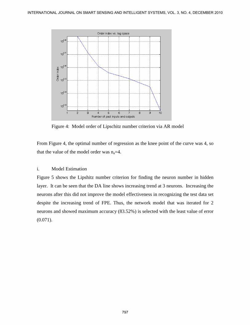
Figure 4: Model order of Lipschitz number criterion via AR model

From Figure 4, the optimal number of regression as the knee point of the curve was 4, so

that the value of the model order was na=4.

i. Model Estimation

Figure 5 shows the Lipshitz number criterion for finding the neuron number in hidden

layer. It can be seen that the DA line shows increasing trend at 3 neurons. Increasing the

neurons after this did not improve the model effectiveness in recognizing the test data set

despite the increasing trend of FPE. Thus, the network model that was iterated for 2

neurons and showed maximum accuracy (83.52%) is selected with the least value of error

(0.071).

797


NAR MODELModel order selection: Lipschitz Number Criteria

(Maximum Iteration=300, stopping criterion=1x10-5, regularization value(D)=0)

78

79

80

81

82

83

84

85

1 2 3 4 5 6 7 8 9 10

Number of Hidden Layer

Acc

urac

y (%

)

-0.00010.01000.02000.03000.04000.05000.06000.07000.08000.09000.1000

Valu

e of

FPE

DA (%) FPE

Figure 5: Plot of diagnostic accuracy and FPE against the number of neurons in the

hidden layer using Lipschitz number criteria via NAR model

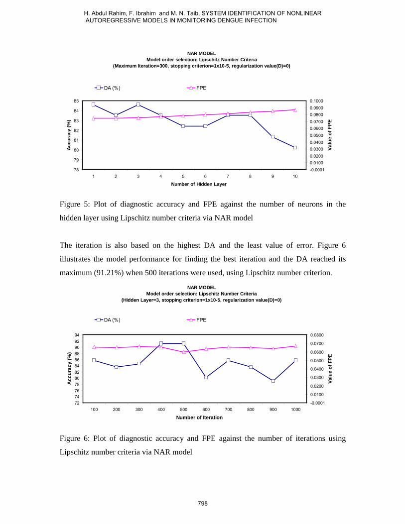
The iteration is also based on the highest DA and the least value of error. Figure 6

illustrates the model performance for finding the best iteration and the DA reached its

maximum (91.21%) when 500 iterations were used, using Lipschitz number criterion.


(Hidden Layer=3, stopping criterion=1x10-5, regularization value(D)=0)

727476788082848688909294

100 200 300 400 500 600 700 800 900 1000

Number of Iteration

Acc

urac

y (%

)

-0.0001

0.0100

0.0200

0.0300

0.0400

0.0500

0.0600

0.0700

0.0800Va

lue

of F

PE

DA (%) FPE

Figure 6: Plot of diagnostic accuracy and FPE against the number of iterations using

Lipschitz number criteria via NAR model

798


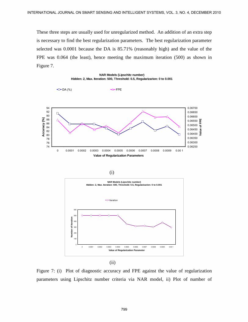
These three steps are usually used for unregularized method. An addition of an extra step

is necessary to find the best regularization parameters. The best regularization parameter

selected was 0.0001 because the DA is 85.71% (reasonably high) and the value of the

FPE was 0.064 (the least), hence meeting the maximum iteration (500) as shown in

Figure 7.

NAR Models (Lipschitz number) Hidden: 2, Max. Iteration: 500, Threshold: 0.5, Regularizarion: 0 to 0.001

7476788082848688909294

0 0.0001 0.0002 0.0003 0.0004 0.0005 0.0006 0.0007 0.0008 0.0009 0.00 1

Value of Regularization Parameters

Acc

urac

y (%

)

0.062500.063000.063500.064000.064500.065000.065500.066000.066500.06700

Valu

e of

FPE

DA (%) FPE

(i)

NAR Models (Lipschitz number) Hidden: 2, Max. Iteration: 500, Threshold: 0.5, Regularizarion: 0 to 0.001

0

100

200

300

400

500

600

0 0.0001 0.0002 0.0003 0.0004 0.0005 0.0006 0.0007 0.0008 0.0009 0.00 1

Value of Regularization Parameter

Num

ber o

f Ite

ratio

n

Iteration

(ii)

Figure 7: (i) Plot of diagnostic accuracy and FPE against the value of regularization

parameters using Lipschitz number criteria via NAR model, ii) Plot of number of

799


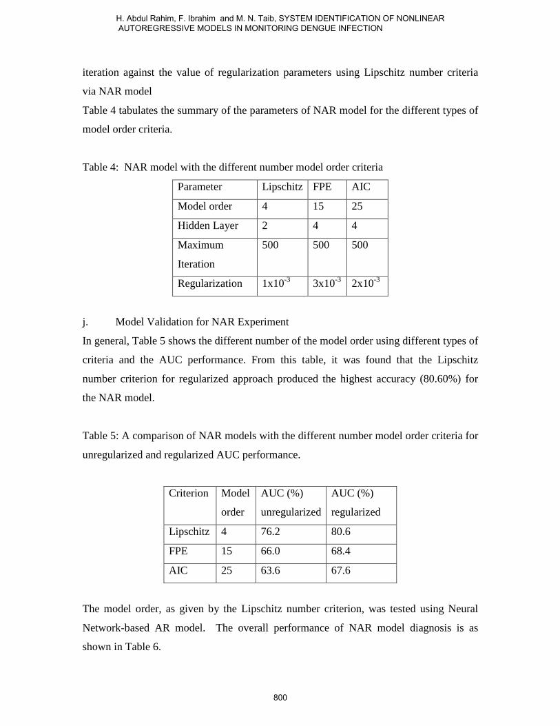
iteration against the value of regularization parameters using Lipschitz number criteria

via NAR model

Table 4 tabulates the summary of the parameters of NAR model for the different types of

model order criteria.

Table 4: NAR model with the different number model order criteria

Parameter Lipschitz FPE AIC

Model order 4 15 25

Hidden Layer 2 4 4

Maximum

Iteration

500 500 500

Regularization 1x10-3 3x10-3 2x10-3

j. Model Validation for NAR Experiment

In general, Table 5 shows the different number of the model order using different types of

criteria and the AUC performance. From this table, it was found that the Lipschitz

number criterion for regularized approach produced the highest accuracy (80.60%) for

the NAR model.

Table 5: A comparison of NAR models with the different number model order criteria for

unregularized and regularized AUC performance.

Criterion Model

order

AUC (%)

unregularized

AUC (%)

regularized

Lipschitz 4 76.2 80.6

FPE 15 66.0 68.4

AIC 25 63.6 67.6

The model order, as given by the Lipschitz number criterion, was tested using Neural

Network-based AR model. The overall performance of NAR model diagnosis is as

shown in Table 6.

800


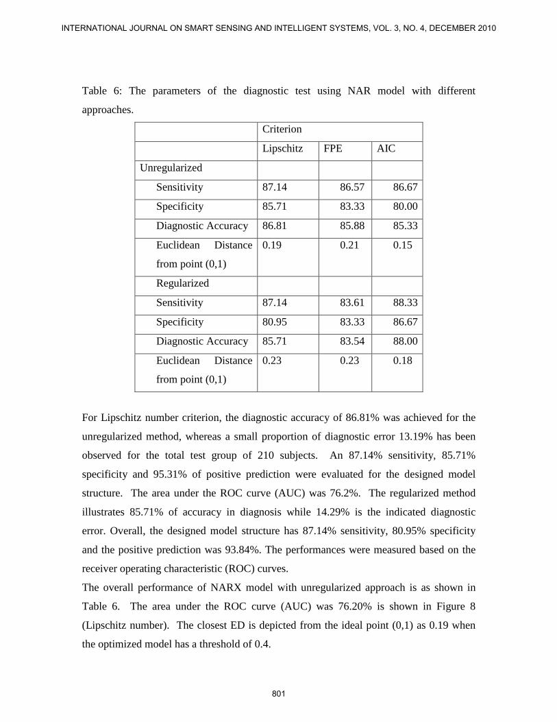
Table 6: The parameters of the diagnostic test using NAR model with different

approaches.

Criterion

Lipschitz FPE AIC

Unregularized

Sensitivity 87.14 86.57 86.67

Specificity 85.71 83.33 80.00

Diagnostic Accuracy 86.81 85.88 85.33

Euclidean Distance

from point (0,1)

0.19 0.21 0.15

Regularized

Sensitivity 87.14 83.61 88.33

Specificity 80.95 83.33 86.67

Diagnostic Accuracy 85.71 83.54 88.00

Euclidean Distance

from point (0,1)

0.23 0.23 0.18

For Lipschitz number criterion, the diagnostic accuracy of 86.81% was achieved for the

unregularized method, whereas a small proportion of diagnostic error 13.19% has been

observed for the total test group of 210 subjects. An 87.14% sensitivity, 85.71%

specificity and 95.31% of positive prediction were evaluated for the designed model

structure. The area under the ROC curve (AUC) was 76.2%. The regularized method

illustrates 85.71% of accuracy in diagnosis while 14.29% is the indicated diagnostic

error. Overall, the designed model structure has 87.14% sensitivity, 80.95% specificity

and the positive prediction was 93.84%. The performances were measured based on the

receiver operating characteristic (ROC) curves.

The overall performance of NARX model with unregularized approach is as shown in

Table 6. The area under the ROC curve (AUC) was 76.20% is shown in Figure 8

(Lipschitz number). The closest ED is depicted from the ideal point (0,1) as 0.19 when

the optimized model has a threshold of 0.4.

801


0.0

0.1

0.2

0.3

0.4

0.5

0.6

0.7

0.8

0.9

1.0

0.0 0.1 0.2 0.3 0.4 0.5 0.6 0.7 0.8 0.9 1.0

1-Specificity

Sens

itivi

ty


(Hidden Layer=2, stopping criterion=1x10-5, regularization value(D)=0)

Figure 8: ROC curve for Lipschitz number criterion using NAR unregularized model

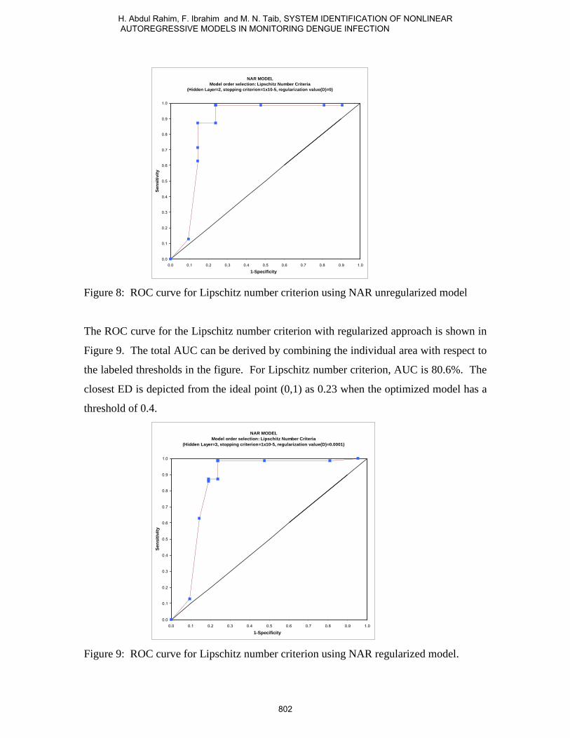
The ROC curve for the Lipschitz number criterion with regularized approach is shown in

Figure 9. The total AUC can be derived by combining the individual area with respect to

the labeled thresholds in the figure. For Lipschitz number criterion, AUC is 80.6%. The

closest ED is depicted from the ideal point (0,1) as 0.23 when the optimized model has a

threshold of 0.4.

0.0

0.1

0.2

0.3

0.4

0.5

0.6

0.7

0.8

0.9

1.0

0.0 0.1 0.2 0.3 0.4 0.5 0.6 0.7 0.8 0.9 1.0

1-Specificity

Sens

itivi

ty


(Hidden Layer=3, stopping criterion=1x10-5, regularization value(D)=0.0001)

Figure 9: ROC curve for Lipschitz number criterion using NAR regularized model.

802


V. CONCLUSIONS

Using SPSS analysis, it was found that the work presented has successfully modeled

heamoglobin status using selected physiological parameters (i.e. gender, vomiting,

weight and day of fever) and BIA parameters (i.e. reactance).

The best model produced by the multilinear regression using four variables (gender,

weight, reactance and vomiting) only yields an accuracy of 43%. This model can be

written as follows: ε+++++= )(19.0.)(047.0)(029.0)(309.1012.6 vomitingreactweightgenderHb

NAR model has produced AUC of 72.60% using Lipschitz number with unregularized

method but the AUC was improve by using the regularized method (80.60%)

The model accuracies in predicting the haemoglobin status, to indicate the dengue

progressions, ranges from 43% (using the multilinear regression) to 80.60% (using NAR

model).

Acknowledgements

The authors are indebted to Universiti Teknologi Malaysia for financial supports.

References

[1] W. H. Organization, Dengue Haemorrhagic fever Diagnosis, treatment,

Prevention, and control, 2nd ed. Geneva: WHO, 1997.

[2] U.G. Kyle, I. Bosaeus, A.D. De Lorenzo, P. Deurenberg, M. Elia, J.M. Gomez,

B.L. Heitmann, L. Kent-Smith, J. Melchior, M. Pirlich, H. Scharfetter, A.M.W.J.

Schols and C. Pichard, "Biolectrical impedance analysis - part1:review of

principles and methods," Clinical Nutrition, vol. 23, pp. 1226-1243, 2004.

[3] F. M. Skae, "Dengue fever in Penang," Br. Med. J, vol. 2, pp. 1581-1582, 1902.

[4] S. C. Gordon, "Dengue: an introduction. In: Rudnick A, Lim TW, Eds. Dengue

Fever Studies in Malaysia Institute for Medical Research Malaysia" Bulletion,

vol. 23, pp. 1-5, 1986.

803


[5] W. C. a. R. Annual Report, "Dengue Haemorrhagic Fever," Dept. of Medical

Microbiology, Fac. of Medicine, University of Malaya, 50603 Kuala Lumpur

Malaysia, 1998.

[6] F. Ibrahim, M.N. Taib, W.A.B. Wan Abas, C.C. Guan, and S. Sulaiman, "A novel

dengue fever (DF) and dengue haemorrhagic fever (DHF) analysis using artificial

neural network," Compu. Methods Programs Biomed., vol. 79, pp. 273-281, 2005.

[7] P.M. Djuric, and S.M. Kay, "Order selection of autoregressive models," IEEE

Trans. On sig. Processing vol. 40, no.11, pp. 2829-2833, 1992.

[8] G.E.P Box, and J.M. Jenkins, "Time series analysis, forecating and control," San

Francisco:Holden Day, 1970.

[9] H. Akaike, "A new look at the statistical model identification," IEEE Trans. On

Automat. Contr., vol. 19, pp. 716-723, 1974.

[10] J. Rissanen, "Modeling by shortest data descriotion," Automatica, vol. 14, pp.

465-478, 1978.

[11] R. L. Kashyap, "Optimal choice of AR and MA parts in autoregressive moving

average models " IEEE Trans. Patt. Anal. Machine Intelligent, vol. 14, pp. 99-

104, 1982.

[12] G. Schwarz, "Estimating the dimension of the model," Ann. Stat., vol. 6, pp. 461-

464, 1978.

[13] K.S. Narenda, and K. Parthasarathy "Identification and control of dynamical

systems using neural networks," IEEE Trans. On Nueral Networks, vol. 1, pp. 4-

27, 1990.

[14] X. He, and H. Asada, "A new method for identifying orders of input-output

models for nonlinear dynamic systems," Proc. of the American Control pp. 2520-

2523, 1993.

[15] M. Norgaard, "Neural network based on system identification toolbox," Technical

Report, 00-E-891, Department of Automation, Technical University of Denmark,

2000.

[16] A. Raganathan, "The Levenberg-Marquardt Algorithm," Georgia Institute of

Technology, unpublished.

[17] S. Roweis, "Levenberg-Marquardt Optimization," Univ. of Toronto, unpublished.

804


[18] K.P. Adlassnig, and W. Scheithauer, "Performance evaluation of medical expert

systems using ROC curves," Compt. Biomed. Res., vol. 22, pp. 297-313, 1989.

[19] J.A. Hanley, and B.J. McNeil, "The meaning and use of the area under a receiver

operating characteristic (ROC) curve," Radiology, vol. 143, pp. 29-36, 1982.

[20] T.J. Downey, D.J. Meyer, R.M. Price, and E.L. Spitznagel "Using the receiver

operating characteristics to asses the performance of neural calssifiers," pp. 3642-

3646, 1999.

[21] B.J. McNeil, and J.A. Hanley, "Statistical approaches to the analysis of receiver

operating characteristic (ROC) curves," Medical Decision Making, vol. 4, pp.

1984, 1984.

[22] F. Ibrahim, "Prognosis of dengue fever and dengue haemorrhagic fever using

bioelectrical impedance," PhD Thesis, Department of Biomedical

Engineering,University of Malaya, July, 2005.

[23] Dengue Haemorrhagic fever Diagnosis, treatment, Prevention, and control, 2nd

ed. Geneva: World Health Organization, 1997.

[24] E. Chungue, J.P. Boutin, and J. Roux, "Antibody capture ELISA for IgM antibody

titration in sera for dengue serodiagnosis and survellance," Research in Virology,

vol. 140, pp. 229-240, 1989.

[25] F. Ibrahim, N.A. Ismail, M.N. Taib and W.A.B. Wan Abas, "Modeling of

hemoglobin in dengue fever and dengue hemorrhagic fever using biolectrical

impedance " Physiol. Meas., vol. 25, pp. 607-615, 2004.

[26] A.R. Herlina, I. Fatimah, and T. Mohd Nasir, "A non-invasive system for

predicting hemoglobin (Hb) in dengue fever (DF) and dengue hemorrhagic fever

(DHF) " in Proc. Int. Conf. on Sensor and New Techniques in Pharmaceutical

and Biomedical Research (ASIASENSE), Kuala Lumpur, 2005.

[27] H. Abdul Rahim, F. Ibrahim, and M.N. Taib, "Modelling of hemoglobin in

dengue infection application," Journal of Electrical Engineering (ELEKTRIKA),

vol. 8, pp. 64-67, 2006.

[28] L. Albert, "Impedance ratio in bioelectrical impedance measurements for body

fluid shift determinitation," in Proc. Proc. of the IEEE 24th Annual Northeast

Bioengineering, 1998, pp. 24-25.

805


806


System identification of nonlinear autoregressive models in monitoring dengue infection

Documents