Synergy–Based Hand Pose Sensing: Optimal Glove Design

Synergy–Based Hand Pose Sensing:Optimal Glove Design∗

Matteo Bianchi†, Paolo Salaris†, Antonio Bicchi†‡

Abstract

In this paper we study the problem of optimally designing glove–based sens-ing devices for hand pose reconstruction to maximize their potential for precision.In a companion paper we studied the problem of maximizing the reconstructionaccuracy of the hand pose from partial and noisy data provided by any given posesensing device (a sensorized “glove”) taking into account the knowledge on howhumans most frequently use their hands in grasping tasks. In this paper we con-sider the dual problem of how to design pose sensing devices, i.e. how and whereto place sensors on a glove, to get maximum information about the actual handposture. We study the optimal design of gloves of different nature, according to aclassification of current sensing technologies adopted in the domain. The objectiveis to provide, for given a priori information and fixed number of sensor inputs, theoptimal design minimizing the reconstruction error statistics (assuming that opti-mal reconstruction algorithms are adopted). Finally, an experimental evaluation ofthe proposed method for optimal design is provided.

1 IntroductionHand Pose Reconstruction (HPR) systems are gaining an increasing importance, sincethey provide useful human–machine interfaces in many applications ranging from tele–robotics, to virtual reality, entertainment and rehabilitation [Dipietro et al., 2008]. Toenable a widespread use of low–cost glove–based HPR, it is crucial to address theproblem of correct hand pose estimation despite the many non–idealities arising, forexample, from the complexity of human hand biomechanics and from measurementinaccuracies.

In [Bianchi et al., 2012b] we describe how to optimize HPR system accuracy — fora given hardware configuration — so as to provide optimal hand pose estimation fromincomplete and imperfect glove data. In the present paper we extend the analysis to theoptimal sensing glove design. The issue is to choose the optimal sensor distribution∗This work is supported by the European Commission under CP grant no. 248587, “THE Hand Embod-

ied”, within the FP7-ICT-2009-4-2-1 program “Cognitive Systems and Robotics” and the ERC AdvancedGrant no. 291166 “SoftHands”: “A Theory of Soft Synergies for a New Generation of Artificial Hands”.

†The Interdept. Research Center “Enrico Piaggio”, University of Pisa, Largo Lucio Lazzarino 1, 56126Pisa, Italy. m.bianchi,p.salaris,[email protected]

‡Department of Advanced Robotics, Istituto Italiano di Tecnologia, via Morego, 30, 16163 Genova, Italy

(a) Slowly adapting (SA)units location.

(b) Fast adapting (FA) unitslocation.

(c) Mechanoreceptor afferent unitsresponding to ≥ 1 joint.

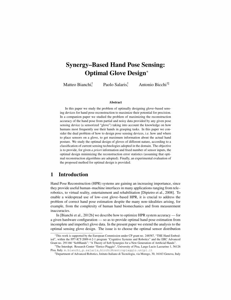
Figure 1: Location of cutaneous mechanoreceptive units in the dorsal skin of the humanhand. Adapted from [Edin and Abbs, 1991], courtesy of the authors.

which maximizes the information on the actual posture. This information, used withthe algorithms proposed in [Bianchi et al., 2012b], will lead to the minimization of thereconstruction error statistics.

That the optimal distribution of sensitivity for HPR is not trivial is strongly sug-gested by the observation of the human example. Indeed, the role of cutaneous informa-tion in kinesthesia and movement control in human hands and fingers has been exten-sively studied in the neuro-physiology literature. For example, [Edin and Abbs, 1991]describe the response to finger movements of cutaneous mechanoreceptors in the dor-sal skin of human hand. The involved mechanoreceptors mainly consist of two types:Fast Adapting afferents of the first type (FAI), and Slow Adapting afferents, of both thefirst and second type (SAI and SAII, respectively). The non–uniform distribution ofthese receptors is shown in figure 1(a) and 1(b). FA units, whose response is localizedto movements about one or, at most, two nearby joints, are found primarily close tojoints; on the other hand SA units, whose discharge rate is influenced by several jointsat the same time, are more uniformly distributed (see figure 1(c)).

These observations suggest that in the human hand sensory system, different ty-pologies of proprioceptive sensors are distributed in the dorsal skin with different densi-ties. This produces a non–uniform map of sensitivities to joint angles, whose functionalmotivation is unclear, but might correspond to the different importance of different el-ementary percepts in building an overall representation of the hand pose. Motivatedby this biological evidence, in this paper we deal with the problem of searching for apreferential distribution and density of different typologies of sensors, so as to optimizethe accuracy of glove–based HPR systems.

The design of sensorized gloves for HPR has received already some attention inthe literature. For example, in [Sturman and Zeltzer, 1993] an investigation of “whole-hand” interfaces for the control of complex tasks is presented, along with the descrip-

tion, design, and evaluation of whole-hand inputs, based on empirical data from users.In [Edmison et al., 2002] authors discussed the properties, advantages, and design as-pects associated with piezoelectric materials for sensing glove design, in an applicationwhere the device is used as a keyboard. Finally, [Chang et al., 2007] explored how tomethodically select a minimal set of hand pose features from optical marker data forHPR. The objective is to determine marker locations on the hand surface that is ap-propriate for classification of hand poses. All the aforementioned approaches rely onad–hoc experimental or qualitative observations: from actual sensor data, locations thatprovide the largest and most useful information on the system are chosen.

More analytical approaches to the problem can be based on the existing literature onoptimal experimental design (see e.g. [Pukelsheim, 2006]). Among optimal design cri-teria, Bayesian methods are ideally suited to contribute to experimental design for errorstatistics minimization (see e.g. [Chaloner and Verdinelli, 1995, Ghosh and Rao, 1996,Bicchi and Canepa, 1994] for a review). On the contrary, non–Bayesian criteria areadopted when the linear Gaussian hypothesis is not fulfilled and/or when the designer’sprimary concern is to minimize worst-case errors rather than error statistics. Crite-ria on explicit worst-case/deterministic bounds on the errors and tools from the the-ory of optimal worst–case/deterministic estimation and/or identification are discussede.g. in [Helmicki et al., 1991, Tempo, 1988, Bicchi, 1992].

It is noteworthy that most results in optimal experimental design refer to the casewhere the number of measurements is redundant or at least equal to the number ofvariables to be estimated. However, the opposite case that fewer sensors are availablethan the hand variables is of main concern in our problem. To circumvent this problem,it is natural to think of exploiting a priori knowledge to disambiguate poses from scarcedata.

In this paper, partially based on [Bianchi et al., 2012a], optimal HPR system designis obtained by relying on results from neuro–scientific studies about hand postures ingrasping tasks [Santello et al., 1998, Schieber and Santello, 2004]. The main findingof these studies is that, despite the hand complexity, simultaneous motion and force ofthe fingers occur in a consistent fashion and is characterized by coordination patterns(“synergies”) that effectively reduce the number of independent hand degrees of free-dom to be controlled. In [Bianchi et al., 2012b], this prior knowledge on how humansmost frequently use their hands is fused with partial and noisy data provided by anygiven HPR device, to maximize reconstruction accuracy. Here, the goal is to charac-terize a design which enables for optimally exploiting – in a Bayesian sense – such ana priori information.

The optimization goals of this paper become particularly relevant when restrictionson the production costs limit both the number and the quality of sensors. In these cases,a careful design is instrumental to obtain good performance. Different technologies andsensor distributions can be considered to realize an HPR device. At the physical level,sensors for HPR gloves can be classified as either lumped (as e.g. a mechanical angularencoder about a joint) or distributed (e.g. a flexible optic fiber running along a fingerfrom base to tip, as in the DataGlove [Zimmerman, 1988]). At the signal level, glovesensors can be coupled (if more than one hand joint angle influences the reading) oruncoupled. Of course, all distributed sensors are coupled, but also lumped sensors canbe coupled due to cross–coupling.

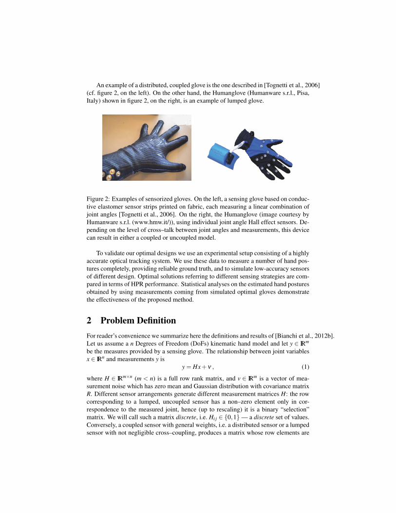
An example of a distributed, coupled glove is the one described in [Tognetti et al., 2006](cf. figure 2, on the left). On the other hand, the Humanglove (Humanware s.r.l., Pisa,Italy) shown in figure 2, on the right, is an example of lumped glove.

Figure 2: Examples of sensorized gloves. On the left, a sensing glove based on conduc-tive elastomer sensor strips printed on fabric, each measuring a linear combination ofjoint angles [Tognetti et al., 2006]. On the right, the Humanglove (image courtesy byHumanware s.r.l. (www.hmw.it/)), using individual joint angle Hall effect sensors. De-pending on the level of cross–talk between joint angles and measurements, this devicecan result in either a coupled or uncoupled model.

To validate our optimal designs we use an experimental setup consisting of a highlyaccurate optical tracking system. We use these data to measure a number of hand pos-tures completely, providing reliable ground truth, and to simulate low-accuracy sensorsof different design. Optimal solutions referring to different sensing strategies are com-pared in terms of HPR performance. Statistical analyses on the estimated hand posturesobtained by using measurements coming from simulated optimal gloves demonstratethe effectiveness of the proposed method.

2 Problem DefinitionFor reader’s convenience we summarize here the definitions and results of [Bianchi et al., 2012b].Let us assume a n Degrees of Freedom (DoFs) kinematic hand model and let y ∈ IRm

be the measures provided by a sensing glove. The relationship between joint variablesx ∈ IRn and measurements y is

y = Hx+ν , (1)

where H ∈ IRm×n (m < n) is a full row rank matrix, and v ∈ IRm is a vector of mea-surement noise which has zero mean and Gaussian distribution with covariance matrixR. Different sensor arrangements generate different measurement matrices H: the rowcorresponding to a lumped, uncoupled sensor has a non–zero element only in cor-respondence to the measured joint, hence (up to rescaling) it is a binary “selection”matrix. We will call such a matrix discrete, i.e. Hi j ∈ {0,1}— a discrete set of values.Conversely, a coupled sensor with general weights, i.e. a distributed sensor or a lumpedsensor with not negligible cross–coupling, produces a matrix whose row elements are

real numbers, i.e., up to rescaling, Hi j ∈ [−1, 1]⊂ IR — a continuous set of values. Inthe following, we will call such a matrix continuous. Finally, a glove employing bothlumped (uncoupled and coupled) and distributed sensors will generate a hybrid mea-surement matrix which consists of a continuous part and a discrete one. Notice that,according to the discussion in figure 1, the human hand sensing distribution could beconsidered to belong to the latter glove class.

In [Bianchi et al., 2012b], the goal is to determine the hand posture, i.e. the jointangles x, by using a set of measures y whose number is lower than the number of DoFsdescribing the kinematic hand model in use. To improve the hand pose reconstruction,we used postural synergy information embedded in the a priori grasp set, which isobtained by collecting a large number N of grasp postures xi, consisting of n DoFs,into a matrix X ∈ IRn×N . This information can be summarized with a covariance matrixPo ∈ IRn×n, which is a symmetric matrix computed as Po = (X−x)(X−x)T

N−1 , where x is amatrix n×N whose columns contain the mean values for each joint angle arranged invector µo ∈ IRn.

Based on the Minimum Variance Estimation (MVE) technique, in [Bianchi et al., 2012b]we obtained the hand pose reconstruction as

x = (P−1o +HT R−1H)−1(HT R−1y+P−1

o µo) , (2)

where matrix Pp = (P−1o +HT R−1H)−1 is the a posteriori covariance matrix. When

R tends to assume very small values, the solution described in (2) might encounternumerical problems. However, by using the Sherman-Morrison-Woodbury formulae,(2) can be rewritten as

x = µo−PoHT (HPoHT +R)−1(Hµo− y) , (3)

and the a posteriori covariance matrix becomes Pp = Po−PoHT (HPoHT +R)−1HPo.The a posteriori covariance matrix, which depends on measurement matrix H, rep-

resents a measure of the amount of information (i.e. observed information) that anobservable variable carries about unknown parameters. In this paper we explore therole of the measurement matrix H on the estimation procedure, providing the optimaldesign of a sensing device able to obtain the maximum amount of the information onthe actual hand posture.

Let us preliminary introduce some useful notations. If M is a symmetric matrix withdimension n, let its Singular Value Decomposition (SVD) be M =UMΣMUT

M , where ΣMis the diagonal matrix containing the singular values σ1(M) ≥ σ2(M) ≥ ·· · ≥ σn(M)of M and UM is an orthogonal matrix whose columns ui(M) are the eigenvectors of M,known as Principal Components (PCs) of M, associated with σi(M). For example, theSVD of the a priori covariance matrix is Po = UPoΣPoUT

Po, with σi(Po) and ui(Po), i =

1,2, . . . ,n, the singular values and the principal components of matrix Po, respectively.

3 Optimal Sensing DesignReferring to model (1), we first analyze the case that individual sensing elements inthe glove can be designed to measure a linear combination of joint angles (i.e. a glove

which can be modeled with a continuous matrix), and provide, for given a priori in-formation and fixed number of measurements, the optimal continuous measurementmatrix, minimizing the reconstruction error statistics. We then consider the case whereeach measure provided by the glove corresponds to a single joint angle (i.e. a glovewhich can be modeled with a discrete matrix). For these types of gloves we determinethe optimal discrete measurement matrix, i.e. which joints should be individually mea-sured in order to optimize the design. Finally, we also define a procedure to obtain theoptimal hybrid measurement matrix.

In the ideal case of noise–free measures (R = 0), Pp becomes zero when H is afull rank n matrix, meaning that available measures contain a complete informationabout the hand posture. In the real case of noisy measures and/or when the numberof measurements m is less than the number of DoFs n, Pp can not be zero. In thesecases, the following problem becomes very interesting: find the optimal matrix H∗

such that the hand posture information contained in the few number of measurementsis maximized. Without loss of generality, we assume H to be full row rank and weconsider the following problem.

Problem 1. Let H be an m× n full row rank matrix with m < n and V1(Po,H,R) :IRm×n→ IR be defined as V1(Po,H,R) = ‖Po−PoHT (HPoHT +R)−1HPo‖2

F , find

H∗ = argminH

V1(Po,H,R)

where ‖ · ‖F denotes the Frobenius norm defined as ‖A‖F =√

tr(AAT ), for A ∈ IRn×n.

To solve problem 1 means to minimize the entries of the a posteriori covariancematrix: the smaller the values of the elements in Pp, the greater is the predictive effi-ciency.

In order to simplify the analysis, in the following we will consider separately theoptimal procedure to define the continuous, discrete and hybrid measurement matrix.

3.1 Continuous Measurement MatrixFor this case, each row of the measurement matrix H is a vector in IRn and hence canbe given as a linear combination of a IRn basis. Without loss of generality, we canuse the principal components of matrix Po, i.e. the columns of the previously definedmatrix UPo , as a basis of IRn. Consequently the measurement matrix can be writtenas H = HeUT

Po, where He ∈ IRm×n contains the coefficients of the linear combinations.

Given that Po =UPoΣPoUTPo

, the a posteriori covariance matrix becomes

Pp =UPo

[Σo−ΣoHT

e (HeΣoHTe +R)−1HeΣo

]UT

Po , (4)

where, for simplicity of notation, Σo ≡ ΣPo .Next sections are dedicated to how to obtain the optimal the continuous measure-

ment matrix both in a numerical and analytical manner. For this purpose, let us intro-duce the set of m× n (with m < n) matrices with orthogonal rows, i.e. satisfying thecondition HHT = Im×m, and let us denote it as Om×n.

3.1.1 Analytical Solutions

We first consider the case of noise–free measures, i.e. R = 0. Let A be a non–negativematrix of order n. It is well known (cf. [Rao, 1964]) that, for any given matrix B ofrank m with m≤ n,

minB‖A−B‖2

F = α2m+1 + · · ·+α

2n , (5)

where αi are the eigenvalues of A, and the minimum is attained when

B = α1w1w1T + · · ·+αmwmwm

T , (6)

where wi are the eigenvector of A associated with αi. In other words, the choice of Bas in (6) is the best fitting matrix of given rank m to A. By using this result we are ableto show when the minimum of (4), hence of

‖Σo−ΣoHTe (HeΣoHT

e )−1HeΣo‖2

F , (7)

can be reached. Let us preliminary observe that the row vectors (hi)e of He can bechosen, without loss of generality, to satisfy the condition (hi)e Σo (h j)e = 0, i 6= j,which implies that the measures are uncorrelated ([Rao, 1964]). Let Om×n denotes theset of m× n matrices, with m < n, whose rows satisfy the aforementioned condition,i.e. the set of matrices with orthonormal rows (HeHT

e = I). By using (5), the minimumof (7) is obtained when (cf. [Rao, 1964])

ΣoHTe (HeΣoHT

e )−1HeΣo = σ1(Σo)u1(Σo)uT

1 (Σo)+ · · ·++σm(Σo)um(Σo)uT

m(Σo) .(8)

Since Σo is a diagonal matrix, ui(Σo) ≡ ei, where ei is the i-th element of the canon-ical basis. Hence, it is easy to verify that (8) holds for He = [Im |0m×(n−m)]. Asa consequence, row vectors (hi) of H∗ are the first m principal components of Po,i.e. (hi) = ui(Po)

T , for i = 1, . . . ,m.From these results, a principal component can be defined as a linear combination of

optimally–weighted observed variables meaning that the corresponding measures canaccount for a maximal amount of variance in the data set. As reported in [Rao, 1964],every set of m optimal measures can be considered as a representation of points inthe best fitting lower dimensional subspace. Thus the first measure gives the bestone–dimensional representation of data set, the first two measures give the best two–dimensional representation, and so on.

In the noisy measurement case, (8) can be rewritten as

ΣoHTe (HeΣoHT

e +R)−1HeΣo−σ1(Σo)u1(Σo)uT1 (Σo)+ · · ·+

+σm(Σo)um(Σo)uTm(Σo) = ∆

In this case, ∆ = 0 can not be attained for any finite H: indeed, for unconstrainedH, infH V1(P0,H,R) would be attained for ‖H‖ → ∞, i.e. for infinite signal–to–noiseratio. The problem can be recast in a well–posed form by imposing a constraint onthe magnitude of the measurement matrix. Up to a possible re–normalization of R, we

can search the optimum design in the set A = {H : HHT = Im}. This problem wasdiscussed and solved in [Diamantaras and Hornik, 1993], showing that, for arbitrarynoise covariance matrix R,

minH∈A

V1(H) =m

∑i=1

σi(Po)

1+σi(Po)/σm−i+1(R)+

n

∑i=m+1

σi(Po) , (9)

which is attained for

H∗ =m

∑i=1

um−i+1(R)uTi (Po) . (10)

Hence, if A consists of all matrices with mutually perpendicular, unit length rows, thefirst m principal components of Po are still the optimal choice for H rows only in caseof uncorrelated noise (i.e. R is a diagonal matrix). For generic noise covariance matri-ces, the optimal choice of matrix H depends also on the principal components of noisematrix R. The alternative case that the solution is sought under a Frobenius norm con-straint on H, i.e. A = {H : ‖H‖F ≤ 1} is discussed in [Diamantaras and Hornik, 1993].

3.1.2 Numerical Solution: Gradient flows on Om×n

In this subsection we describe a different approach to the solution of problem 1, whichconsists of constructing a differential equation whose trajectories converge to the de-sired optimum. The method lends itself directly to efficient numerical implementations.Although a closed–form solution has been proposed in the previous subsection, the nu-merical solution considered here is very useful when constraints are imposed on themeasurement structure (as they will be for instance in the hybrid case), where closedform solutions are not applicable.

The following proposition describes an algorithm that minimizes the cost functionV1(Po,H,R), providing the gradient flow which will be useful in the method of steepestdescent.

Proposition 1. The gradient flow for the function V1(Po,H,R) : IRm×n→ IR is given by,

H =−∇‖Pp‖2F = 4

[P2

p PoHTΣ(H)

]T, (11)

where Σ(H) = (HPoHT +R)−1.

Proof. See Appendix.

Let us observe that rows of matrix H can be chosen, without loss of generality,such that HiPoHT

j = 0, i 6= j which imply that measures are uncorrelated, i.e. satisfyingthe condition HHT = Im. Of course, in case of noise–free sensors, this constraint isnot strictly necessary. On the other hand, in case of noisy sensors, the minimum ofV1(Po,H,R) can not be obtained since it represents a limit case that can be achievedwhen H becomes very large (i.e. an infimum) and hence increasing the signal–to–noiseratio.

A reasonable solution for the constrained problem will be provided by using theRosen’s gradient projection method for linear constraints [Rosen, 1960], which is based

on projecting the search direction onto the subspace tangent to the constraint. Hence,given the steepest descent direction for the unconstrained problem, this method consistson finding the direction with the most negative directional derivative which satisfies theconstraint on the structure of the matrix H, i.e. HHT = Im. This can be obtained byusing the projection matrix

W = In−HT (HHT )−1H , (12)

and then projecting the unconstrained gradient flow (11) into the subspace tangent tothe constraint, obtaining the search direction

s = ∇‖Pp‖2F W . (13)

Having the search direction for the constrained problem, the gradient flow is givenby

H =−4[P2

p PoHTΣ(H)

]TW (14)

where Σ(H) = (HPoHT +R)−1. The gradient flow (11) guarantees that the optimalsolution H∗ will satisfy H∗(H∗)T = Im, if H(0) satisfies H(0)H(0)T = Im, i.e. H ∈Om×n.

Notice that both Om×n and V1(Po,H,R) are not convex, hence the problem could nothave a unique minimum. However, in case of noise–free measures, the invariance of thecost function w.r.t. changes of basis, i.e. V1(Po,H,0) =V1(Po,MH,0), with M ∈ IRm×m

a full rank matrix, suggests that there exists a subspace in IRm×n where the optimumis achieved. Hence, considering results reported in previous section (see (8)), we canconclude that gradient (11) with R = 0 becomes zero when rows of matrix H are anylinear combination of the first m principal components of the a priori covariance matrixPo. This does not happen in case of noisy measures with generic noise covariancematrix and gradient (14) becomes zero only for a particular matrix H which dependsalso on the principal components of the matrix R (see (10)). Notice that, according toprevious analytical results, when the noise covariance matrix is diagonal, then gradient(14) becomes zero only if matrix H consists of the first m principal components of Po.

3.2 Discrete Measurement MatrixWhen each measure y j, j = 1, . . . ,m provided by the glove corresponds to a single jointangle xi, i = 1, . . . ,n, the problem is to find the optimal choice of m joints or DoFs tobe measured. Measurement matrix becomes in this case a full row rank matrix whereeach row is a vector of the canonical basis, i.e. matrices which have exactly one nonzeroentry in each row.

Let Nm×n denote the set of m×n element–wise non–negative matrices, then Pm×n =Om×n ∩Nm×n, where Pm×n is the set of m× n permutation matrices (see lemma 2.5in [Zavlanos and Pappas, 2008]). This result implies that if we restrict H to be or-thonormal and element–wise non–negative, we get a permutation matrix. In this paperwe extend this result in IRm×n, obtaining matrices which have exactly one nonzero entryin each row. Hence, the problem to solve becomes:

Problem 2. Let H be a m× n matrix with m < n, and V1(Po,H,R) : IRm×n → IR bedefined as V1(Po,H,R) = ‖Po − PoHT (HPoHT + R)−1HPo‖2

F , find the optimal mea-surement matrix

H∗ = argminH

V1(Po,H,R)

s.t. H ∈Pm×n .

In this case a closed–form solution is not available. Nonetheless, as the modelused to describe the kinematics of the hand has usually a low number of DoFs, theoptimal choice H∗ can be computed by exhaustion, substituting all possible sub–sets ofm vectors of the canonical basis in the cost function V1(Po,H,R). In the next section,a more general approach to compute the optimal matrix will be provided in order toobtain a result also when a model with a large number of DoFs is considered.

3.2.1 Numerical Solution: Gradient Flows on Pm×n

In this section, we describe an alternative approach to the solution of problem 2 basedon a gradiental method. Once again, although the enumeration approach can solve theproblem in practical cases, the numerical solution based on the method here presentedwill be useful in the hybrid case.

A numerical solution for problem 2 can be obtained following a method presentedin [Zavlanos and Pappas, 2008], which consists in defining a function V2(P) with P ∈IRn×n that forces the entries of P to be as positive as possible, thus penalizing negativeentries of H. In this paper, we extend this function to measurement matrices H ∈ IRm×n

with m < n. Consider a function V2 : Om×n→ IR as

V2(H) =23

tr[HT (H− (H ◦H))

], (15)

where A ◦ B denotes the Hadamard or element–wise product of the matrices A =(ai j) and B = (bi j), i.e. A ◦ B = (ai jbi j). The gradient flow of V2(H) is given by([Zavlanos and Pappas, 2008])

H =−H[(H ◦H)T H−HT (H ◦H)

], (16)

which minimizes V2(H) converging to a permutation matrix if H(0) ∈ Om×n.The two gradient flows given by (11) and (16), both defined on the space of or-

thogonal matrices, tend to minimize their cost functions, respectively. By combiningthese two gradient flows we can achieve a solution for Problem 2. An interesting resultapplies to the dynamics of the convex combination of these gradients, which can bestated as follows.

Theorem 1. Let H ∈ IRm×n with m < n be the measurement process matrix and as-sume that H(0) ∈ Om×n. Moreover, suppose that H(t) satisfies the following matrixdifferential equation,

H = 4(1− k)[P2

p PoHTΣ(H)

]TW+

+ k H[(H ◦H)T H−HT (H ◦H)

], (17)

where k ∈ [0, 1] is a positive constant, W = In−HT (HHT )−1H and Σ(H) = (HPoHT +R)−1. For sufficiently large k, limt→∞ H(t) = H∞ exists and approximates a permuta-tion matrix that also (locally) minimizes the squared Frobenius norm of the a posterioricovariance matrix, ‖Pp‖2

F .

The proof of this theorem is a direct extension of results in [Zavlanos and Pappas, 2008],and is omitted for brevity.

As in most numerical optimization algorithms, the non–convex nature of the costfunction and of the support set implies the need for multi–start approaches. A possibletechnique to help converge towards the global optimum consists in increasing k duringthe search procedure (cf. [Zavlanos and Pappas, 2008]).

3.3 Hybrid Measurement MatrixUp to re–arranging the sensor numbering, we can write a hybrid measurement matrixHc,d ∈ IRm×n as

Hc,d =

[HcHd

],

where Hc ∈ IRmc×n defines the mc rows of the continuous part, whereas Hd ∈Pmd×n

describes the md single–joint measurements of the discrete part, with mc +md = m.Neither the closed–form solution valid for the continuous measurement matrix, nor theexhaustion method used for discrete measurements are applicable in the hybrid case.Therefore, to optimally determine the hybrid measurement matrix, we will recur togradient–based iterative optimization algorithms.

By combining the continuous and discrete gradient flows, previously defined in (11)and (16), respectively, and constraining the solution in the sub–set Hc,d = {Hc,d :Hc,dHT

c,d = Im}, we obtain

Hc,d = 4(1− k)[P2

p PoHTc,dΣ(Hc,d)

]TW+

+ k Hd[(Hd ◦ Hd)

T Hd− HTd (Hd ◦ Hd)

], (18)

where k ∈ [0, 1] is a positive constant, Pp = Po−PoHTc,d(Hc,dPoHT

c,d +R)−1Hc,dPo, W =

In−HTc,d(Hc,dHT

c,d)−1Hc,d , Σ(Hc,d) = (Hc,dPoHT

c,d +R)−1, and

Hd =

[0mc×n

Hd

].

Starting from any initial guess matrix Hc,d ∈Hc,d , the gradient flow defined in (18)remains in the sub–set Hc,d and, on the basis of Theorem 1, it converges toward ahybrid measurement matrix, (locally) minimizing the squared Frobenius norm of the aposteriori covariance matrix. Multi–start strategies have to be used to circumvent theproblem of local minima.

When noise is not negligible, without constraining the solution in Hc,d by W , thegradient search method of (18) would tend to produce measurement matrices whosecontinuous parts, Hc, are very large in norm. This is an obvious consequence of thefact that, for a fixed noise covariance R, larger measurement matrices H would producean apparently higher signal–to–noise ratio in (1).

4 On the Practical Realization of Optimal Sensing De-vices

In this section we describe some feasible solutions to realize a device which can bemodeled by the previously obtained optimal continuous, discrete and hybrid measure-ment matrices, to achieve a trade–off between accuracy, cost, usability and ease tomade, on the basis of the current technology.

Lumped, uncoupled sensing devices, which generate a discrete measurement ma-trix, are probably the easiest to be implemented, as they require to individually measuresingle joints according to the optimal measurement matrix. Common sensing strategiesinclude Hall–effect (e.g. Humanglove) or piezoresistive sensors (e.g. CyberGlove, byCyberGlove System LLC, San Jose, CA – USA), directly placed on the joints to bemeasured, hence obtaining a lumped device. However some difficulties can occur dueto coupling between non–measured and measured joints and cross–coupling betweensensors. This last problem becomes particularly relevant when the optimality requiresto place sensors on adjacent joints. To circumvent these drawbacks, attention mustbe paid on the ergonomics of sensor physical support as well as appropriate sensorshielding (e.g. with Hall–effect transducer).

On the other hand, distributed sensors, which generate an optimal continuous ma-trix, should provide measurements in terms of optimally weighted linear combina-tions of the contributions of different DoFs, according to the principal componentsof the a priori data and of noise covariance matrix. Of course, under a technologi-cal viewpoint, the weight of each measured DoF can be approximated with a givenlevel of accuracy due to the particular application and sensor technology. The liter-ature ([Dipietro et al., 2008]) describes at least two main technologies to implementdistributed sensing strategies. A first one is based on resistive ink printed on flexibleplastic bends that follow the movement of hand joints (e.g. PowerGlove by Mattel Inc.,El Segundo, CA–USA). In this case a change in the configuration of the joints resultsin a change of the overall resistance. It is possible to weight each joint contributionin a different manner by suitably modifying its electrical resistance (e.g. increasingor decreasing the section of the printed segments corresponding to different joints). Asecond technology adopts capacitive sensors (as e.g. in the Didjiglove by DijiglovePty. Ltd., Melbourne, AUS), i.e. two layers of conductive polymer separated by a di-electric, which overlap different joints. By bending the sensors, a change in the overallcapacitance will be produced. Also in this case we can weight each joint differentlyby varying the thickness and the type of dielectric surface as well as the electrode sur-face overlapping. Finally, the above discussed technologies (lumped, uncoupled anddistributed) can be adopted and combined in an efficient manner to optimally realizedevices which can be modeled by a hybrid measurement matrix.

5 Experimental Setup for A Priori and Validation DataTo validate our optimal design, we performed some simulations using measurementsfrom human posture data acquired by means of an optical tracking system. As de-scribed in the following, this data contains joint angles for a large set of grasping poses,

and can be regarded as a reasonable reference to compare reconstruction outcomes.These values were used to simulate optimally designed gloves, i.e. they were combinedeach time to provide a measurement outcome according to the continuous, hybrid anddiscrete measurement matrix, i.e. H∗c , H∗c,d and H∗d , respectively, as well as to other non–optimal measurement matrix. Without loss of generality, for hand pose reconstruction

DoFs DescriptionTA Thumb AbductionTR Thumb RotationTM Thumb MetacarpalTI Thumb InterphalangealIA Index AbductionIM Index MetacarpalIP Index Proximal

MM Middle MetacarpalMP Middle ProximalRA Ring AbductionRM Ring MetacarpalRP Ring ProximalLA Little abductionLM Little MetacarpalLP Little Proximal

Figure 3: Kinematic model of the hand with 15 DoFs.

we adopt the 15 DoFs model also used in [Santello et al., 1998, Gabiccini et al., 2011]and reported in figure 3. The model DoFs are: 4 DoFs for the thumb, i.e. TR, TA, TM,TI (Thumb Rotation, Abduction, Metacarpal, Interphalangeal); 3 DoFs for the index,i.e. IA, IM, IP (Index Abduction, Metacarpal, Proximal Interphalangeal); 2 DoFs forthe middle, i.e. MM, MP (Middle Metacarpal, Proximal Interphalangeal); 3 DoFs forthe ring, i.e. RA, RM, RP (Ring Abduction, Metacarpal, Proximal Interphalangeal);3 DoFs for the little, i.e. LA, LM, LP (Little Abduction, Metacarpal, Proximal Inter-phalangeal). Notice that the middle finger has no abduction since it is considered the“reference finger” in the sagittal plane of the hand.

An optical motion capture system (Phase Space, San Leandro, CA – USA) with19 active markers was used to collect a large number of static grasp positions (seefigure 4). Subject AT (M,26) performed all the grasps of the 57 imagined objectsdescribed in [Santello et al., 1998]; these data were acquired twice to define a set of114 a priori data.

The disposition of the markers on the hand refers to [Fu and Santello, 2010]. Weused four markers for the thumb and three markers for each of the rest of the fingers.Three markers were also placed on the dorsal surface of the palm to define a localreference system SH (see figure 3). The positions of the markers, which were sampled

Figure 4: Experimental setup for hand pose acquisition with Phase Space system.

at 480 Hz, are given referring to the global reference system SMC (which is directlydefined during the calibration of the acquisition system).

An additional set of Np = 54 grasp poses was performed by subject LC (26,M).Subject was asked to perform some imagined grasped object poses contained in the apriori data set and also some new postures which identify basic grasping configura-tions of the hand (e.g. precision and power grasp) 1. None of the subjects had physicallimitations that would affect the experimental outcomes. Data collection from subjectsin this study was approved by the University of Pisa Institutional Review Board. Thelatter set of poses will be referred hereinafter as validation set, since these poses can beassumed to represent accurate reference angular values for hand pose configurations,given the high accuracy provided by the optical system to detect markers (the amount ofstatic marker jitter is inferior than 0.5 mm, usually 0.1 mm) and assuming a linear cor-relation (due to skin stretch) between marker motion around the axes of rotation of thejoint and the movement of the joint itself [Zhang et al., 2003]. The validation set wasthen used to simulate optimal gloves. According to the number of measures, we consid-ered from the postures in this set only the joint values resulting from the optimizationprocedure, assuming to select them in a linear weighted combination (continuous mea-surement matrix), individually (discrete measurement matrix) or combining discreteand continuous measurements (hybrid measurement matrix). Since all the DoFs ofthe postures in the validation set are known, we compare the reconstructed hand con-figurations obtained from simulated optimal glove measures with the reference ones.The same procedure is used for hand pose reconstruction achieved starting from nonoptimal measures provided by Hs, which is described in the following section.

1These hand posture acquisitions are available at http://handcorpus.org/

6 Application of Optimal Glove Design TechniquesIn this section we analyze the main features of hand pose sensing devices, whose designis determined on the basis of the optimal procedures proposed in previous sections.First, based on the covariance matrix of the a priori data set (cf. Section 5), we giveexamples of optimal distributions of sensors in terms of continuous, hybrid and discretemeasurement matrix in case of noise-free measures. Furthermore, we characterize howthe information available by measurement process increases with the minimization ofthe squared Frobenius norm of the a posteriori covariance matrix as well as with anincreasing number of measures.

Second, we show how the optimal design improves the estimation algorithms pro-posed in the companion paper [Bianchi et al., 2012b] and briefly described in Section 2of this manuscript. In [Bianchi et al., 2012b], we tested the proposed estimations al-gorithms using discrete matrix Hs, which models a lumped, uncoupled sensing device,providing the individual measures of five metacarpal joints, i.e. TM, IM, MM, RM andLM. In this section, we compare the hand posture reconstruction obtained by Hs withthe one obtained by using the optimal matrix H∗d with the same number of measure-ments. Improvements on the estimation of hand postures in case of both noise–freeand noisy measures are shown. In case of noisy measures, an additional random noisewas artificially added on each measure. A zero–mean, Gaussian noise with standarddeviation 0.122 rad ( 7◦) was chosen based on data about common technologies andtools used to measure hand joint positions [Simone et al., 2007], thus obtaining a noisecovariance matrix R≈ diag(0.0149).

Finally, for the sake of completeness, we compare hand pose estimation perfor-mance achievable with the optimal design of corresponding to continuous, hybrid anddiscrete measurement matrix, considering the same number of measures. The purposeof this comparison is to analyze and discuss benefits of each type of optimal sensordistribution w.r.t. the other ones.

6.1 Sensor Distributions Based on Continuous, Discrete and Hy-brid Measurement Matrices

As shown in Section 3, the optimal choice H∗c of the measurement matrix H ∈ IRm×n isrepresented by the first m principal components (synergies) of the a priori covariancematrix Po. Figure 5 shows the optimal sensor distribution related to a continuous mea-surement matrix which furnishes a number of measures up to three. In this case, eachmeasure is given as yk = ∑

ni=1 wi xi with k = 1, . . . ,m. In figure 5 a representation, in

grayscale, of the absolute value of wi, is reported: the greater is the absolute coefficientwi, the darker is the color of that joint.

The optimal measurement matrix H∗d , for a number of noise–free measures m rang-ing from 1 to 14, is reported in table 1. Notice that, H∗d does not have an incrementalbehavior, especially in case of few measures. In other words, the set of DoFs whichhave to be chosen in case of m measures does not necessarily contain all the set ofDoFs chosen for m− 1 measures. Moreover, noise randomness can slightly changewhich DoFs have to be measured compared with the noise–free case.

Figure 5: Optimal sensing distribution according to the first three PCs of Po, whichcorrespond to the rows of the optimal continuous measurement matrix up to three mea-sures. The greater is the absolute coefficient wi of the joint angle in the PC and hencein each measure yk = ∑

ni=1 wi xi with k = 1,2,3, the darker (in grayscale) is the color

of that joint. For representation purposes only, we consider the absolute value of thecoefficient of the i-th joint in the PC to be normalized w.r.t. the maximum absolutevalue of the coefficients that can be achieved all over the joints.

For the sake of completeness, table 2 shows also an example of optimal measure-ment matrix H∗c,d for a number of noise–free measures m ranging from 1 to 14, whereonly the first measure is continuous (i.e. mc = 1). Of course, table 2 shows only theselected DoFs of each discrete measure. However, results obtained with the gradient

m TA TR TM TI IA IM IP MM MP RA RM RP LA LM LP V1

1 X 7.12 ·10−2

2 X X 2.39 ·10−2

3 X X X 6.59 ·10−3

4 X X X X 3.30 ·10−3

5 X X X X X 1.90 ·10−3

6 X X X X X X 5.32 ·10−4

7 X X X X X X X 2.92 ·10−4

8 X X X X X X X X 1.98 ·10−4

9 X X X X X X X X X 1.30 ·10−4

10 X X X X X X X X X X 6.86 ·10−5

11 X X X X X X X X X X X 2.70 ·10−5

12 X X X X X X X X X X X X 1.40 ·10−5

13 X X X X X X X X X X X X X 3.39 ·10−6

14 X X X X X X X X X X X X X X 1.32 ·10−6

Table 1: Optimal measured DoFs for H∗d with an increasing number of noise–freemeasures m (cf. figure 3).

m = 1+md TA TR TM TI IA IM IP MM MP RA RM RP LA LM LP V1

2 X 1.81 ·10−2

3 X X 5.49 ·10−3

4 X X X 2.68 ·10−3

5 X X X X 1.27 ·10−3

6 X X X X X 3.64 ·10−4

7 X X X X X X 2.46 ·10−4

8 X X X X X X X 1.58 ·10−4

9 X X X X X X X X 9.10 ·10−5

10 X X X X X X X X X 4.95 ·10−5

11 X X X X X X X X X X 2.09 ·10−5

12 X X X X X X X X X X X 8.70 ·10−6

13 X X X X X X X X X X X X 3.02 ·10−6

14 X X X X X X X X X X X X X 4.59 ·10−7

Table 2: Optimal measured DoFs for the discrete part of the optimal hybrid matrixH∗c,d with only one continuous measure (mc = 1) and with an increasing number ofnoise–free measures m (cf. figure 3).

flow (18) proposed in Section 3.3 show that the elements of the continuous part of H∗c,dcorresponding to DoFs measured by the discrete part, tend to be zero. For instance,if m = 2 with mc = 1, matrix H∗c,d furnishes two measures: the discrete one gives theangle of RM DoF (see table 2), while the continuous part is a linear combination of alljoints angle but RM one. Indeed, the RM angle is perfectly known, i.e. we have themaximum information available on that DoF and hence, the continuous measure has tofurnish information only on the other DoFs.

Let us quantify the information made available by the optimal measurement pro-

cess through the square Frobenius norm of the a posteriori covariance matrix (V1).Figure 6 shows the values of V1 for increasing number m of noise–free measures. Thebest performance is obtained by the continuous measurement matrix, as expected andthe observed information is always the greatest one. Indeed, principal componentsare considered the optimal measures for the representation of points in the best fittinglower dimensional subspace [Rao, 1964]. The optimal hybrid measurement matrix we

0 1 2 3 4 5 6 7 8 9 10 11 12 13 14 150

0.02

0.04

0.06

0.08

0.1

0.12

0.14

0.16

0.18

0.2

V 1(Po,H

,0)

m

Hc , R=0Hd , R=0Hc,d , R=0

2 3 4 50

0.005

0.01

0.015

0.02

V1(Po,H,0)

m

Figure 6: Squared Frobenius norm of the a posteriori covariance matrix with noise–freemeasures in case of H∗c , H∗d and H∗c,d (mc = 1) with an increasing number of noise-freemeasures. A zoomed detail of the graph is shown for m = 2,3,4,5 measures.

consider for this analysis has only a continuous measure, the first one. For this rea-son, in figure 6, the same value for V1 is observed for both hybrid and continuous casewhen only one measure (m = 1) is considered, hence leading to same performance.Then, increasing the number of discrete measures, performance of hybrid matrix tendsto be close to the discrete one (see the zoomed detail in figure 6), even if observedinformation for hybrid measurement matrix is always greater than the observed infor-mation for the discrete measurement matrix. Notice that V1 values decrease with thenumber of measures, tending to be zero (cf. figure 6) for all three cases. This fact istrivial because increasing the measurements, the uncertainty on the measured variablesis reduced. When all the measured information is available V1 assumes zero value withperfectly accurate measures in all three cases. In case of noisy measures, V1 valuesdecrease with the number of measures tending to a value which is larger, depending onthe level of noise.

For noise–free measures, we analyze how much V1 reduces with the number ofmeasurements w.r.t. the value it assumes for zero measures (Pp ≡ P0). In terms of mea-surement process, i.e. from the observability viewpoint, a reduced number of measurescoinciding with the first three principal components enable for ' 97% reduction ofthe squared Frobenius norm of the a posteriori covariance matrix. An analogous re-sult can be found also under the controllability point of view. In [Santello et al., 1998]authors state that three postural synergies are crucial in grasp pre–shaping since theytake into account for ' 90% of pose variability in grasping tasks. The above reportedresult seems logic considering the duality between observability and controllability.

2 5 3 5 4 5 5 50

0.005

0.01

0.015

0.02

0.025

0.03

0.035

0.04

0.045

0.05

m

V 1(Po,H

,0)

H*d

Hs

Figure 7: Squared Frobenius norm for the a posteriori covariance matrix of Hs whichmodels a sensing device, providing the individual measures of five (m = 5) metacarpaljoints, i.e. TM, IM, MM, RM and LM, and H∗d with m = 2, 3, 4, 5 measures, in case ofnoise–free measures (see table 2).

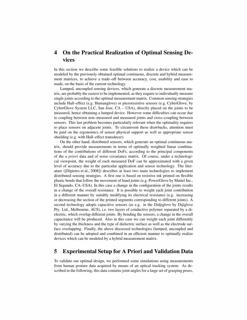
Finally, let us consider figure 7 and 8, where squared Frobenius norm for the a posteri-ori covariance matrix of Hs with m = 5 measures, and H∗d with m = 2,3,4,5 measures,in case of noise-free and noisy measures, respectively, is reported. Notice that, V1 issignificantly smaller in the optimal case, even when a reduced number of measures isconsidered, leading to a better estimation performance also with an inferior numberof measured DoFs w.r.t. Hs. For sake of space, in Subsection 7.1, we report only theestimation comparison when both Hs and H∗d provide five measures.

2 5 3 5 4 5 5 50

0.01

0.02

0.03

0.04

0.05

m

V1(P

o,H

,R)

H*

d

Hs

Figure 8: Squared Frobenius norm for the a posteriori covariance matrix of Hs whichmodels a sensing device, providing the individual measures of five (m = 5) metacarpaljoints, i.e. TM, IM, MM, RM and LM with m = 5 measures, and H∗d with m = 2, 3, 4, 5measures, in case of noisy measures.

7 Experimental ResultsIn this section, we compare the hand posture reconstructions, considering m = 5 mea-sures provided by matrix Hs and by optimal matrix H∗d in case of both noise–free andnoisy measures. Second, we analyze HPR performance for the tree sensing typolo-gies of optimal sensor distributions corresponding to the three optimal measurementmatrices.

7.1 Hs vs. H∗d with m = 5

In figure 9, sensor locations related to matrix Hs and H∗d (with noise–free and noisymeasures), are represented. For the comparison, measures are provided by grasp dataacquired with the optical tracking system as described in Section 5 (see also [Bianchi et al., 2012b]for more details), where degrees of freedom to be measured are chosen on the basis ofoptimization procedure outcomes, while the entire pose is recorded to produce accuratereference posture.

In figure 10, some reconstructed poses with MVE algorithm are reported by us-ing both Hs and H∗d , with and without additional noise. Under a qualitative point ofview, what is noticeable is that reconstructed poses are not far from the real ones forboth measurement matrices, even if the pose error ei =

1n ∑

ni=1 |xi− xi| is smaller for

the optimal case. Moreover, it may happen that some poses are estimated in a bettermanner using Hs and vice versa, even if, as we will show in next subsections, from astatistical point of view, H∗d provides best average performance. Indeed, MVE methodsare thought to minimize error statistics rather than worst–case sensing errors related toparticular poses [Bicchi and Canepa, 1994].

Figure 9: Measured joints (highlighted in color) for matrix Hs, and H∗d , with and with-out noise (cf. figure 3).

In the following, as evaluation indices, the average pose estimation error and av-erage estimation error for each estimated DoF are used. Maximum errors are alsoreported. These errors as well as statistical tools are chosen according to the ones con-sidered in [Bianchi et al., 2012b]. Statistical differences between estimated pose andjoint errors obtained with different glove designs are computed by using classic tools,after having tested for normality and homogeneity of variances assumption on samples(through Lilliefors’ composite goodness–of–fit test and Levene’s test, respectively).Standard two–tailed t–test (hereinafter referred as Teq ) is used in case of both the as-

sumptions are met, a modified two–tailed T–test is exploited (Behrens–Fisher problem,using Satterthwaite’s approximation for the effective degrees of freedom, hereinafterreferred as Tneq ) when variance assumption is not verified and finally a non parametrictest is adopted for the comparison (Mann–Whitney U–test, hereinafter referred as U )when normality hypothesis fails. Significance level of 5% is assumed and p-values lessthan 10−4 are posed equal to zero.

7.1.1 Noise–Free Measures

In terms of average absolute estimation pose errors ([◦]), performance obtained withH∗d is always better than the one exhibited by Hs (3.67±0.93 vs. 6.69±2.38). More-over, H∗d exhibits smaller maximum error than the one achieved with Hs (i.e. 8.25◦ forH∗d vs. 13.18◦ for Hs). Statistical difference between results from Hs and H∗d is found(p ' 0, Tneq). In table 3 average absolute estimation errors with their correspondingstandard deviations for each DoF are reported. For the estimated DoFs, performancewith H∗d is always better or not statistically different from the one referred to Hs. Max-imum estimation errors underline cases where Hs furnishes smaller values and viceversa, since they strictly depend on particular poses.

7.1.2 Noisy Measures

In case of noise, performance in terms of average absolute estimation pose errors ([◦])obtained with H∗d is better than the one exhibited by Hs (5.96±1.42 vs. 8.18±2.70).Moreover, maximum pose error with H∗d is the smallest (9.30◦ vs. 15.35◦ observed withHs). Statistical difference between results from Hs and H∗d is found (p=0.001, Tneq). Intable 4 average absolute estimation error with standard deviations are reported for eachDoF. Also in this case, for the estimated DoFs, performance with H∗d is always better ornot statistically different from the one referred to Hs. Maximum estimation errors withH∗d are usually inferior to the ones obtained with Hs. The MVE method seems to givemore accurate estimates for certain DoFs (e.g. TA, IA, RA, LA, for Hs and MP, RA,RM, LP for H∗d ) with noise than without noise even if in the latter case, the averageabsolute pose estimation error is the smallest one.

It should be noticed that the MVE method guarantees that the mean squared normof the joint error vector (i.e. the Mean Squared Error, MSE = 1

N ∑Ni=1 ‖x− x‖2, where

N represents the number of predictions) is minimized, but not necessarily the value ofeach single component. Same applies with noise: indeed, some particular joints have alower error with noise than without noise, yet the overall error norm (across all joints) isalways higher if noise is present. Indeed, if the joint angles of both the estimations andthe reference poses are in degrees, the MSE with the optimal measurement matrix H∗d(Hs) is 522 (1583) in case of noise–free measures and 948 (1992) in case of noise, henceit increases with noise. The fact that noise happens to reduce the error in some jointsis a statistically insignificant case, that has occurred with the validation set reportedin the paper. Using other validation sets, we have obtained estimates where noisereduces the error of different individual joints, or increases all components: however,as theory predicts, the overall mean square error vector is always increased by noise.The whole argument rests on the fact that the validation sets are samples from the same

Figure 10: Hand pose reconstructions MVE algorithm by using matrix Hs which allowsto measure T M, IM, MM, RM and LM and matrix H∗d which allows to measure TA,MM, RP, LA and LM (cf. figure 3). In color the real hand posture whereas in white theestimated one. The pose error is given by ei =

1n ∑

ni=1 |xi− xi|.

distribution, of which the a priori set is assumed to provide a statistically accuratedescription.

DoFMean Error [�] Hs vs. H⇤d Max Error [�]

Hs H⇤d p-values Hs H⇤dTA⌦ 10.74±8.45 0 0 31.65 0TR 7.16±4.54 6.84±4.75 0.72 ⇧ 19.50 20.13

TM� 0 2.17±2.21 0 0 13.04TI 4.81±3.68 5.33±4.16 0.64 19.68 15.15IA 11.96±5.33 10.55±5.65 0.14 26.35 26.15

IM� 0 4.02±3.43 0 0 16.01IP 13.26±7.06 5.42±6.44 0 27.46 43.86

MM�⌦ 0 0 – 0 0MP 12.35±7.75 4.90±2.91 0 ‡ 29.94 9.91RA 3.45±2.43 3.82±2.94 0.73 9.51 12.68

RM� 0 6.68±3.68 0 0 16.01RP⌦ 13.40±9.65 0 0 39.33 0LA⌦ 11.33±5.87 0 0 24.47 0

LM�⌦ 0 0 – 0 0LP 11.94±9.52 6.27±3.97 0.0002 36.58 16.63

1 �����������������0p-values

� indicates a DoF measured with Hs⌦ indicates a DoF measured with H⇤d

Table 3: Average estimation errors and standard devia-tions for each DoF [�] for the simulated acquisition con-sidering Hs and H⇤d both with five noise–free measures.Maximum errors are also reported as well as p-valuesfrom the evaluation of DoF estimation errors between Hsand H⇤d . ⇧ indicates Teq test. ‡ indicates Tneq test. Whenno symbol appears near the tabulated values, U test isused. Bold value indicates no statistical difference be-tween the two methods under analysis at 5% significancelevel. When the difference is significative, values are re-ported with a 10�4 precision. p-values less than 10�4 areconsidered equal to zero. Symbol “–” is used for thoseDoFs which are measured by both Hs and H⇤d .

7.1.2 Noisy Measures

In case of noise, performance in terms of average absolute estimation pose errors ([�])obtained with H⇤d is better than the one exhibited by Hs (5.96±1.42 vs. 8.18±2.70).Moreover, maximum pose error with H⇤d is the smallest (9.30� vs. 15.35� observed withHs). Statistical difference between results from Hs and H⇤d is found (p=0.001, Tneq). Intable 4 average absolute estimation error with standard deviations are reported for each

Table 3: Average estimation errors and standard deviations for each DoF [◦] for thesimulated acquisition considering Hs and H∗d both with five noise–free measures. Max-imum errors are also reported as well as p-values from the evaluation of DoF estimationerrors between Hs and H∗d . � indicates Teq test. ‡ indicates Tneq test. When no symbolappears near the tabulated values, U test is used. Bold value indicates no statisticaldifference between the two methods under analysis at 5% significance level. Whenthe difference is significative, values are reported with a 10−4 precision. p-values lessthan 10−4 are considered equal to zero. Symbol “–” is used for those DoFs which aremeasured by both Hs and H∗d .

7.2 Estimation Performance Comparison for Optimal Sensor De-signs

As previously shown, the observed information quantified through V1 (squared Frobe-nius norm of the a posteriori covariance matrix) is greatest for continuous case, whilehybrid case provides better performance than the discrete one. Here, we analyze howthese differences affect the reconstruction pose accuracy. To accomplish this goal, weconsider as an example the case of three noise–free measures (m = 3). For the hybridcase, only the first measure is continuous (i.e. mc = 1 and md = 2).

DoFMean Error [�] Hs vs. H⇤d Max Error [�]

Hs H⇤d p-values Hs H⇤dTA⌦ 6.7±5.62 4.87±3.57 0.19 23.35 15.93TR 7.65±5.57 7.54±5.00 0.91 ⇧ 27.46 22.73

TM� 2.81±1.75 2.63±1.90 0.61 ⇧ 7.2 8.78TI 6.08±4.63 5.42±4.74 0.32 19.6 19.10IA 10.74±5.6 11.52±5.81 0.32 27.31 28.46

IM� 4.15±3.17 6.91±5.00 0.003 11.66 21.49IP 14.61±7.93 6.61±6.01 0 31.85 38.07

MM�⌦ 4.59±3.08 4.71±3.19 0.77 11.43 15.72MP⌦ 13.71±8.07 4.08±2.98 0 ‡ 37.61 13.71RA 3.12±2.37 3.28±2.45 0.71 9.18 9.37

RM� 4.03±3.07 6.30±4.72 0.01 ‡ 12.94 12.91RP 16.78±11.07 6.89±3.82 0 ‡ 50.66 16.34LA 8.97±5.11 9.86±5.45 0.38 ⇧ 20.86 21.48

LM�⌦ 3.82±3.05 4.82±4.30 0.44 11.33 14.26LP⌦ 14.64±9.68 3.94±2.95 0 48.61 11.03

1 �����������������0p-values

� indicates a DoF measured with Hs⌦ indicates a DoF measured with H⇤d

Table 4: Average estimation errors and standard devia-tions for each DoF [�] for the simulated acquisition con-sidering Hs and H⇤d both with five noisy measures. Maxi-mum errors are also reported as well as p-values from theevaluation of DoF estimation errors between Hs and H⇤d . ⇧indicates Teq test. ‡ indicates Tneq test. When no symbolappears near the tabulated values, U test is used. Boldvalue indicates no statistical difference between the twomethods under analysis at 5% significance level. Whenthe difference is significative, values are reported with a10�4 precision. p-values less than 10�4 are consideredequal to zero. Symbol “–” is used for those DoFs whichare measured by both Hs and H⇤d .

with H⇤d are usually inferior to the ones obtained with Hs. The MVE method seemsto give more accurate estimates for certain DoFs (e.g. TA, IA, RA, LA, for Hs andMP, RA, RM, LP for H⇤d ) with noise than without noise even if in the latter case, theaverage absolute pose estimation error is the smallest one. This depends on differentfactors: the measured joint angles, the a priori covariance matrix and the amplitudeand the structure of the measurement noise. How these factors interact to determine

Table 4: Average estimation errors and standard deviations for each DoF [◦] for thesimulated acquisition considering Hs and H∗d both with five noisy measures. Maximumerrors are also reported as well as p-values from the evaluation of DoF estimation errorsbetween Hs and H∗d . � indicates Teq test. ‡ indicates Tneq test. When no symbol appearsnear the tabulated values, U test is used. Bold value indicates no statistical differencebetween the two methods under analysis at 5% significance level. When the differenceis significative, values are reported with a 10−4 precision. p-values less than 10−4 areconsidered equal to zero. Symbol “–” is used for those DoFs which are measured byboth Hs and H∗d .

To enable for a correct comparison, we compute average absolute estimation poseerrors ([◦]) only on estimated DoFs, disregarding each time those joints whose valuesare perfectly known since individually measured (i.e. RM, RP for both H∗c,d and H∗d andTA for H∗d ). Performance obtained with H∗c is always better than the one exhibited byH∗c,d and H∗d (5.09±1.6 vs. 6.16±1.64 and 6.61±1.89, respectively). Statistical differ-ence between H∗c and H∗d and between H∗c and H∗c,d is found (p ' 0, U). No statisticaldifference is observed between H∗c,d and H∗d (p = 0.19, Teq). Moreover, H∗c exhibits thesmallest maximum error: 9.95 vs. 11.30 and 11.73 for H∗c,d and H∗d , respectively.

DoF Mean Error [�] p-values Max Error [�]H⇤c H⇤c,d H⇤d H⇤c vs. H⇤d H⇤c vs. H⇤c,d H⇤c,d vs. H⇤d H⇤c H⇤c,d H⇤d

TA� 4.44±4.85 4.60±4.48 0 0 0.69 0 17.19 15.83 0TR 5.64±3.96 5.79±3.86 7.28±4.68 0.08 0.84⇧ 0.13 17.11 16.65 18.86TM 2.69±1.89 2.40±1.90 2.07±1.88 0.04 0.34 0.35 8.61 8.77 10.39TI 3.72±2.80 4.02±3.03 4.36±3.34 0.28⇧ 0.70 0.73 13.95 12.83 14.18IA 12.04±6.00 12.13±6.23 12.05±6.40 0.83 1 0.87 29.32 30.24 30.56IM 4.43±4.09 6.84±5.64 9.81±7.35 0 0.02 0.05 16.79 21.01 25.22IP 4.39±4.64 5.17±6.63 5.09±6.53 0.77 0.64 0.98 30.81 45.43 44.63

MM 3.68±2.70 7.36±4.92 8.76±5.40 0 0 0.07 11.04 21.40 23.34MP 3.66±2.57 4.63±2.87 4.54±2.94 0.1⇧ 0.07⇧ 0.87⇧ 14.26 10.80 10.88RA 3.40±2.41 3.42±2.56 3.49±2.54 0.91 0.96 0.91 9.44 10.00 9.88

RM�⌦ 5.41±2.58 0 0 0 0 – 11.85 0 0RP�⌦ 4.62±3.76 0 0 0 0 – 16.29 0 0

LA 10.12±4.41 12.26±4.59 10.96±6.52 0.43‡ 0.01⇧ 0.24‡ 19.74 20.89 25.85LM 3.84±2.96 5.26±3.44 4.79±4.72 0.55 0.01 0.07 10.76 18.10 19.64LP 3.79±3.02 6.18±4.32 6.09±4.24 0.004 0.003 0.88 13.53 17.29 16.94

1 �������������������0p-values� indicates a DoF measured with H⇤d⌦ indicates a DoF measured with the discrete part of H⇤c,d .

Table 5: Average estimation errors and standard deviations for each DoF [�] forthe simulated estimation considering H⇤c , H⇤c,d and H⇤d , with three noise-free mea-sures. Maximum errors are also reported as well as p-values from the evaluationof DoF estimation errors between the continuous, hybrid and discrete design. ⇧indicates Teq test. ‡ indicates Tneq test. When no symbol appears near the tabulatedvalues, U test is used. Bold value indicates no statistical difference between thetwo methods under analysis at 5% significance level. When the difference is sig-nificative, values are reported with a 10�4 precision. p–values less than 10�4 areconsidered equal to zero. Symbol “–” is used for those DoFs which are measuredby both H⇤d and the discrete part of H⇤c,d .

8 ConclusionsIn this paper, optimal design of sensing glove has been proposed on the basis of theminimization of the a posteriori covariance matrix as it results from the estimationprocedure described in [Bianchi et al., 2012]. Optimal solution are described for thecontinuous, discrete and hybrid case.

In the continuous sensing measurement matrix case, basically correspondingto distributed sensing devices, optimal measures are individuated by principal com-ponents of the a priori covariance matrix, thus suggesting the importance of posturalsynergies not only for hand control.

The reconstruction performance obtained by combining the estimation techniqueproposed in [Bianchi et al., 2012] and the optimal design proposed in this paper is sig-nificantly improved if compared with non–optimal measure case. Therefore, [Bianchi et al., 2012]and this paper provide a complete procedure to enhance the performance and for a moreeffective development of sensorization systems for robotic hands and active touch sens-ing systems. These techniques can be useful in a wide range of applications, ranging

Table 5: Average estimation errors and standard deviations for each DoF [◦] for thesimulated estimation considering H∗c , H∗c,d and H∗d , with three noise-free measures.Maximum errors are also reported as well as p-values from the evaluation of DoF esti-mation errors between the continuous, hybrid and discrete design. � indicates Teq test.‡ indicates Tneq test. When no symbol appears near the tabulated values, U test is used.Bold value indicates no statistical difference between the two methods under analysisat 5% significance level. When the difference is significative, values are reported witha 10−4 precision. p–values less than 10−4 are considered equal to zero. Symbol “–” isused for those DoFs which are measured by both H∗d and the discrete part of H∗c,d .

In table 5 average absolute estimation errors with their corresponding standard de-viations for each DoF are reported. For the estimated DoFs, performance with H∗c isalways better or not statistically different from the one referred to H∗c,d or H∗d . Only forTM joint performance with H∗d is better than H∗c even if p–value is close to the signif-icance level. Finally, no statistical difference is observed between H∗c,d and H∗d . Sameconsiderations still work for maximum estimation errors.

Conclusions we can drawn are that, even if the values for V1 (see figure 6) differnot so much for the three cases, the continuous measurement matrix provides the bestpose reconstruction performance. Of course, the trade–off between performance, costand ease to design should be taken into account to determine whether and how well aparticular design suits a particular application.

8 ConclusionsIn this paper, optimal design of sensing glove has been proposed on the basis of theminimization of the a posteriori covariance matrix as it results from the estimationprocedure described in [Bianchi et al., 2012b]. Optimal solution are described for thecontinuous, discrete and hybrid case.

In the continuous measurement matrix case, basically corresponding to distributedsensing devices, optimal measures are individuated by principal components of the apriori covariance matrix, thus suggesting the importance of postural synergies not onlyfor hand control.

The reconstruction performance obtained by combining the estimation techniqueproposed in [Bianchi et al., 2012b] and the optimal design proposed in this paper is sig-nificantly improved if compared with non–optimal measure case. Therefore, [Bianchi et al., 2012b]and this paper provide a complete procedure to enhance the performance and for a moreeffective development of sensorization systems for robotic hands and active touch sens-ing systems. These techniques can be useful in a wide range of applications, rangingfrom virtual reality to tele-robotics and rehabilitation. Moreover, by optimizing thenumber and location of sensors the production costs can be further reduced withoutloss of performance, thus increasing device diffusion.

Further work will be dedicated to the physical implementation of the here proposedoptimal designs as well as defining optimal calibration strategies.

AcknowledgmentsAuthors gratefully acknowledge Marco Santello and Lucia Pallottino for the inspiringdiscussion and useful suggestions.

References[Bianchi et al., 2012a] Bianchi, M., Salaris, P., and Bicchi, A. (2012a). Synergy–based

optimal design of hand pose sensing. In IEEE-RSJ International Conference onIntelligent Robots and Systems.

[Bianchi et al., 2012b] Bianchi, M., Salaris, P., and Bicchi, A. (2012b). Synergy-based hand pose sensing: Performance enhancement. The International Journalof Robotics Research. Submitted.

[Bicchi, 1992] Bicchi, A. (1992). A criterion for optimal design of multiaxis forcesensors. Journal of Robotics and Autonomous Systems, 10(4):269–286.

[Bicchi and Canepa, 1994] Bicchi, A. and Canepa, G. (1994). Optimal design of mul-tivariate sensors. Measurement Science and Technology (Institute of Physics Jour-nal “E”), 5:319–332.

[Chaloner and Verdinelli, 1995] Chaloner, K. and Verdinelli, I. (1995). Bayesian ex-perimental design: A review. Statistical Science, 10:273–304.

[Chang et al., 2007] Chang, L. Y., Pollard, N. S., Mitchell, T. M., and Xing, E. P.(2007). Feature selection for grasp recognition from optical markers. In Intel-ligent Robots and Systems, 2007. IROS 2007. IEEE/RSJ International Conferenceon, pages 2944–2950.

[Diamantaras and Hornik, 1993] Diamantaras, K. and Hornik, K. (1993). Noisy prin-cipal component analysis. Measurement‘93, pages 25 – 33.

[Dipietro et al., 2008] Dipietro, L., Sabatini, A., and Dario, P. (2008). A survey ofglove-based systems and their applications. Systems, Man, and Cybernetics, PartC: Applications and Reviews, IEEE Transactions on, 38(4):461 –482.

[Edin and Abbs, 1991] Edin, B. B. and Abbs, J. H. (1991). Finger movement re-sponses of cutaneous mechanoreceptors in the dorsal skin of the human hand. Jour-nal of neurophysiology, 65(3):657–670.

[Edmison et al., 2002] Edmison, J., Jones, M., Nakad, Z., and Martin, T. (2002). Usingpiezoelectric materials for wearable electronic textiles. In Wearable Computers,2002. (ISWC 2002). Proceedings. Sixth International Symposium on, pages 41 – 48.

[Fu and Santello, 2010] Fu, Q. and Santello, M. (2010). Tracking whole hand kine-matics using extended kalman filter. In Engineering in Medicine and Biology So-ciety (EMBC), 2010 Annual International Conference of the IEEE, pages 4606 –4609.

[Gabiccini et al., 2011] Gabiccini, M., Bicchi, A., Prattichizzo, D., and Malvezzi, M.(2011). On the role of hand synergies in the optimal choice of grasping forces.Auton. Robots, 31(2-3):235–252.

[Ghosh and Rao, 1996] Ghosh, S. and Rao, C. R. (1996). Review of optimal bayes de-signs. In Design and Analysis of Experiments, volume 13 of Handbook of Statistics,pages 1099 – 1147. Elsevier.

[Helmicki et al., 1991] Helmicki, A. J., Jacobson, C. A., and Nett, C. N. (1991). Con-trol oriented system identification: a worst-case/deterministic approach in h∞. Au-tomatic Control, IEEE Transactions on, 36(10):1163 –1176.

[Pukelsheim, 2006] Pukelsheim, F. (2006). Optimal Design of Experiments (Clas-sics in Applied Mathematics) (Classics in Applied Mathematics, 50). Society forIndustrial and Applied Mathematics, Philadelphia, PA, USA.

[Rao, 1964] Rao, C. R. (1964). The use and interpretation of principal componentanalysis in applied research. The Indian journal of statistic, 26:329 – 358.

[Rosen, 1960] Rosen, J. B. (1960). The gradient projection method for nonlinear pro-gramming. part i. linear constraints. Journal of the Society for Industrial and Ap-plied Mathematics, 8(1):181 – 217.

[Santello et al., 1998] Santello, M., Flanders, M., and Soechting, J. F. (1998). Posturalhand synergies for tool use. The Journal of Neuroscience, 18(23):10105 – 10115.

[Schieber and Santello, 2004] Schieber, M. H. and Santello, M. (2004). Hand func-tion: peripheral and central constraints on performance. Journal of Applied Physi-ology, 96(6):2293 – 2300.

[Simone et al., 2007] Simone, L. K., Sundarrajan, N., Luo, X., Jia, Y., and Kamper,D. G. (2007). A low cost instrumented glove for extended monitoring and functionalhand assessment. Journal of Neuroscience Methods, 160(2):335–348.

[Sturman and Zeltzer, 1993] Sturman, D. J. and Zeltzer, D. (1993). A design methodfor “whole-hand” human-computer interaction. ACM Trans. Inf. Syst., 11(3):219–238.

[Tempo, 1988] Tempo, R. (1988). Robust estimation and filtering in the presence ofbounded noise. Automatic Control, IEEE Transactions on, 33(9):864 –867.

[Tognetti et al., 2006] Tognetti, A., Carbonaro, N., Zupone, G., and De Rossi, D.(2006). Characterization of a novel data glove based on textile integrated sensors. InAnnual International Conference of the IEEE Engineering in Medicine and BiologySociety, EMBC06, Proceedings., pages 2510 – 2513.

[Zavlanos and Pappas, 2008] Zavlanos, M. M. and Pappas, G. J. (2008). A dynamicalsystems approach to weighted graph matching. Automatica, 44(11):2817 – 2824.

[Zhang et al., 2003] Zhang, X., Lee, S., and Braido, P. (2003). Determining fingersegmental centers of rotation in flexion-extension based on surface marker mea-surement. Journal of Biomechanics, 36:1097 – 1102.

[Zimmerman, 1988] Zimmerman, T. G. (1982). Optical flex sensor. Patent US4542291, Sep. 29.

A AppendixThis appendix is devoted to the derivation of the gradient equation given in proposi-tion 1.

Proof of Proposition 1 The Frobenius norm of a matrix A ∈ IRn×n is given as

‖A‖F =√

tr(AT A) =

√n

∑i=1

σ2i ,

and hence,‖Po−PoHT (HPoHT +R)−1HPo‖2

F = tr(PTp Pp) (19)

where Pp = Po − PoHT (HPoHT + R)−1HPo. To find the gradient flow, we need tocompute

∂ tr(PTp Pp)

∂H= tr

(∂ (PT

p Pp)

∂H

)= tr

(∂PT

p

∂HPp +PT

p∂Pp

∂H

)=

= tr

(∂PT

p

∂HPp

)+ tr

(PT

p∂Pp

∂H

)= 2tr

(PT

p∂Pp

∂H

), (20)

as ∂ (XY) = (∂X)Y+X(∂Y) and tr(AT ) = tr(A). Moreover, from differentiation rulesof expressions w.r.t. a matrix X, we have ∂X−1 =−X−1(∂X)X−1 and hence, assumingΣ(H) = (HPoHT +R)−1, we obtain

∂Pp

∂H=−Po

[(∂H)T

Σ(H)H +HT(

∂Σ(H)

∂HH +Σ(H)∂ H

)]Po =

=−Po[(∂H)T

Σ(H)H−HT (Σ(H)

(∂HPoHT+

+HPo(∂H)T )Σ(H)H +Σ(H)∂H

)]Po . (21)

Substituting (21) in (20) and by using a well note trace property (tr(A+B) = tr(A)+tr(B)) we obtain

∂ tr(PTp Pp)

∂H= 2

[− tr(PT

p Po(∂H)TΣ(H)HPo)+ tr(PT

p PoHTΣ(H)∂HPoHT

Σ(H)HPo)+

+ tr(PTp PoHT

Σ(H)HPo(∂H)TΣ(H)HPo)− tr(PT

p PoHTΣ(H)∂HPo)

].

(22)

As tr(AB) = tr(BA), we obtain

∂ tr(PTp Pp)

∂H= 2

[− tr((∂H)T

Σ(H)HPoPTp Po)+ tr(PoHT

Σ(H)HPoPTp PoHT

Σ(H)∂H)+

+ tr((∂H)TΣ(H)HPoPT

p PoHTΣ(H)HPo)− tr(PoPT

p PoHTΣ(H)∂H)

](23)

and as tr(AT ) = tr(A) we have

∂ tr(PTp Pp)

∂H= 2

[− tr(PT

o PpPTo HT

Σ(H)T∂H)+ tr(PoHT

Σ(H)HPoPTp PoHT

Σ(H)∂H)+

+ tr(PTo HT

Σ(H)T HPTo PpPT

o HTΣ(H)T

∂H)− tr(PoPTp PoHT

Σ(H)∂H)],

(24)

whence,

∂ tr(PTp Pp)

∂H= 2

[−PT

o PpPTo HT

Σ(H)T +PoHTΣ(H)HPoPT

p PoHTΣ(H)+

+PTo HT

Σ(H)T HPTo PpPT

o HTΣ(H)T −PoPT

p PoHTΣ(H)

]=

= 2[(PoHT

Σ(H)H− I)PoPTp PoHT

Σ(H)+(PTo HT

Σ(H)T H− I)PTo PpPT

o HTΣ(H)T ] .

(25)

Matrices Pp, Po and Σ(H) are symmetric, and hence, for this particular case we obtain

∂ tr(PTp Pp)

∂H=−4

[P2

p PoHTΣ(H)

]T, (26)

with Σ(H) = (HPoHT +R)−1.