Syncopation: Unifying Music Theory and Perception Thesis submitted in partial fulfilment of the requirements of the University of London for the Degree of Doctor of Philosophy Chunyang Song June 2014 Department of Electronic Engineering, Queen Mary, University of London

Welcome message from author
This document is posted to help you gain knowledge. Please leave a comment to let me know what you think about it! Share it to your friends and learn new things together.
Transcript
Syncopation: Unifying Music
Theory and Perception
Thesis submitted in partial fulfilment
of the requirements of the University of London
for the Degree of Doctor of Philosophy
Chunyang Song
June 2014
Department of Electronic Engineering,
Queen Mary, University of London

I, Chunyang Song, confirm that the research included within this thesis
is my own work or that where it has been carried out in collaboration with,
or supported by others, that this is duly acknowledged below and my con-
tribution indicated. Previously published material is also acknowledged
below.
I attest that I have exercised reasonable care to ensure that the work
is original, and does not to the best of my knowledge break any UK law,
infringe any third party’s copyright or other Intellectual Property Right,
or contain any confidential material.
I accept that the College has the right to use plagiarism detection
software to check the electronic version of the thesis.
I confirm that this thesis has not been previously submitted for the
award of a degree by this or any other university.
The copyright of this thesis rests with the author and no quotation
from it or information derived from it may be published without the prior
written consent of the author.
Signature:
Date:
Details of collaboration and publications:
• Song C, Simpson AJR, Harte CA, Pearce MT, Sandler MB (2013)
Syncopation and the Score. PLoS ONE 8(9): e74692.
This work is covered in Chapter 4.
• Song C, Harte CA, Simpson AJR, Sandler MB, Syncopation models:
do they measure up? Submitted to Music Perception in May, 2014.
This work is covered in Chapters 3 and 5.
2
Abstract
Syncopation is a fundamental feature of rhythm in music. However, the
relationship between theory and perception is currently not well under-
stood. This thesis is concerned with characterising this relationship and
identifying areas where the theory is incomplete. We start with a review of
relevant musicological background and theory. Next, we use psychophysi-
cal data to characterise the perception of syncopation for simple rhythms.
We then analyse the predictions of current theory using this data and iden-
tify strengths and weaknesses in the theory. We then introduce further
psychophysical data which characterises the perception of syncopation for
simple rhythms at different tempi. This leads to revised theory and a new
model of syncopation that is tempo-dependent.
3

Acknowledgements
I would like to thank my supervisors Mark Sandler and Marcus Pearce for
their guidance and support. I would also like to acknowledge the Joint
Programme College Scholarship that funded my studies and especially Yue
Chen for extending the funding to support my writing up.
Special thanks to Mark Plumbley for always making time to talk and
for helping me several times with my travel to conferences and research
visits. Many thanks to Tanya Gold for proof-reading my thesis and to
Michael Tautschnig for advice on mathematical notation.
I would like to give my biggest thanks to Chris Harte, not only for
always making the time to discuss research with me and giving me good
advice, but also for being my greatest support and mentor. Without
his enduring encouragement I could not possibly have the confidence and
persistence to drive myself to the finish line.
I also owe a great deal of thanks to Andy Simpson, the sweetest unan-
ticipated surprise along my Ph.D journey, for pointing me in the right
direction and helping me find so much insight and passion in my work.
His help really put a rocket under my research in my final year and for
this I will always be very grateful.
I must also thank all the people who participated in my listening tests
(in alphabetical order): Alice, Alo, Andy, Bogdan, Boris, Brecht, Chris,
Dan, Dimitrios, Daniele, Elio, Emmanouil, George, Han, Holger, Jordan,
Katerina, Magda, Mike, Steve and Sonia.
Many thanks also to my friends in Georgia Tech who helped me so
much during my three-month research visit: Qingfen, Jiechao, Weibin,
Ruofeng, Aron and Mason; and Yi for taking care of me during my trip
to SMPC in Toronto.
Special thanks to my dear “104 gang”, especially Siying, Tian and
Yading for their huge support and great company. I will always remember
4

the times when we worked together till late, and when we said we would
work hard but ended up nut-chatting the whole night. I appreciate that
you guys tried all sorts to help me with writing up, such as hiding my
phone and working in shift to watch over me. Thanks particularly to Sonia
for being my writing-up buddy and cheering every step of my progress with
me.
Finally, I am very grateful to my parents and entire family members
in China, and also my family in UK: grandma, grandpa, ma, pa, and all
my awesome Leavening branch, for their everlasting support and love.
5

Contents
Abstract . . . . . . . . . . . . . . . . . . . . . . . . . . . . . . . . 3
1 Introduction . . . . . . . . . . . . . . . . . . . . . . . . . . . . 17
1.1 Motivations . . . . . . . . . . . . . . . . . . . . . . . . . . 18
1.2 Methodology . . . . . . . . . . . . . . . . . . . . . . . . . 21
1.3 Goals and objectives . . . . . . . . . . . . . . . . . . . . . 23
1.4 Thesis outline . . . . . . . . . . . . . . . . . . . . . . . . . 24
2 Syncopation in music theory . . . . . . . . . . . . . . . . . 27
2.1 Fundamentals of rhythm . . . . . . . . . . . . . . . . . . . 27
2.1.1 Rhythm . . . . . . . . . . . . . . . . . . . . . . . . 27
2.1.2 Beat . . . . . . . . . . . . . . . . . . . . . . . . . . 31
2.1.3 Meter . . . . . . . . . . . . . . . . . . . . . . . . . 31
2.1.4 Tempo . . . . . . . . . . . . . . . . . . . . . . . . . 35
2.2 Definitions for syncopation . . . . . . . . . . . . . . . . . . 37
2.2.1 Violation of the regular beat salience . . . . . . . . 37
2.2.2 Off-beat . . . . . . . . . . . . . . . . . . . . . . . . 38
2.2.3 Transformation of meter . . . . . . . . . . . . . . . 40
2.2.4 Polyrhythm . . . . . . . . . . . . . . . . . . . . . . 41
2.3 Overview of syncopation models . . . . . . . . . . . . . . . 42
2.3.1 Categories of models . . . . . . . . . . . . . . . . . 43
2.3.2 Capabilities of models . . . . . . . . . . . . . . . . 44
2.4 Summary . . . . . . . . . . . . . . . . . . . . . . . . . . . 45
3 Review of syncopation models . . . . . . . . . . . . . . . . 46
3.1 Background . . . . . . . . . . . . . . . . . . . . . . . . . . 46
3.1.1 Sequences . . . . . . . . . . . . . . . . . . . . . . . 46
3.1.2 Rhythm in continuous time . . . . . . . . . . . . . 48
3.1.3 Discrete time representation . . . . . . . . . . . . . 49
3.1.4 Metrical hierarchy . . . . . . . . . . . . . . . . . . 52
6
3.2 Syncopation models . . . . . . . . . . . . . . . . . . . . . . 55
3.2.1 Longuet-Higgins and Lee 1984 (LHL) . . . . . . . . 55
3.2.2 Pressing 1997 (PRS) . . . . . . . . . . . . . . . . . 58
3.2.3 Toussaint 2002 ‘Metric Complexity’ (TMC) . . . . 61
3.2.4 Sioros and Guedes 2011 (SG) . . . . . . . . . . . . 62
3.2.5 Keith 1991 (KTH) . . . . . . . . . . . . . . . . . . 65
3.2.6 Toussaint 2005 ‘Off-Beatness’ (TOB) . . . . . . . . 66
3.2.7 Gomez 2005 ‘Weighted Note-to-Beat Distance’ (WNBD) 67
3.3 Summary . . . . . . . . . . . . . . . . . . . . . . . . . . . 68
4 Syncopation and the score . . . . . . . . . . . . . . . . . . . 70
4.1 Experiment 1: Score . . . . . . . . . . . . . . . . . . . . . 70
4.1.1 Participants . . . . . . . . . . . . . . . . . . . . . . 71
4.1.2 Stimuli . . . . . . . . . . . . . . . . . . . . . . . . . 71
4.1.3 Procedure . . . . . . . . . . . . . . . . . . . . . . . 74
4.2 Results . . . . . . . . . . . . . . . . . . . . . . . . . . . . . 75
4.2.1 6/8 is more syncopated than 4/4 . . . . . . . . . . 75
4.2.2 Polyrhythms are more syncopated . . . . . . . . . . 75
4.2.3 Missing down-beats result in syncopation . . . . . . 77
4.2.4 Switching component order affects syncopation . . . 78
4.3 Discussion . . . . . . . . . . . . . . . . . . . . . . . . . . . 81
4.3.1 4/4 versus 6/8 . . . . . . . . . . . . . . . . . . . . . 81
4.3.2 Missing down-beats . . . . . . . . . . . . . . . . . . 82
4.3.3 Possible interpretation of 6/8 as 3/4 . . . . . . . . 83
4.3.4 Polyrhythms . . . . . . . . . . . . . . . . . . . . . . 84
4.4 Summary . . . . . . . . . . . . . . . . . . . . . . . . . . . 85
5 Evaluation of the models . . . . . . . . . . . . . . . . . . . . 86
5.1 Dataset 1 . . . . . . . . . . . . . . . . . . . . . . . . . . . 86
5.2 Evaluation results . . . . . . . . . . . . . . . . . . . . . . . 89
5.3 Discussion: strengths and weaknesses of models . . . . . . 90
5.3.1 Hierarchical models . . . . . . . . . . . . . . . . . . 90
5.3.2 Off-beat models . . . . . . . . . . . . . . . . . . . . 95
5.3.3 Classification models . . . . . . . . . . . . . . . . . 97
5.3.4 General discussion . . . . . . . . . . . . . . . . . . 98
5.4 Summary . . . . . . . . . . . . . . . . . . . . . . . . . . . 98
7

6 Tempo affects syncopation . . . . . . . . . . . . . . . . . . . 100
6.1 Background . . . . . . . . . . . . . . . . . . . . . . . . . . 101
6.1.1 Tactus perception and tempo . . . . . . . . . . . . 101
6.1.2 Tempo limits of tactus and meter perception . . . . 102
6.1.3 Dynamic meter perception influenced by tempo . . 103
6.1.4 Hypotheses for tempo effects on syncopation . . . . 106
6.2 Experiment 2: Tempo . . . . . . . . . . . . . . . . . . . . 108
6.2.1 Participants . . . . . . . . . . . . . . . . . . . . . . 108
6.2.2 Stimuli . . . . . . . . . . . . . . . . . . . . . . . . . 108
6.2.3 Procedure . . . . . . . . . . . . . . . . . . . . . . . 111
6.3 Results . . . . . . . . . . . . . . . . . . . . . . . . . . . . . 111
6.3.1 Syncopation is a function of tempo . . . . . . . . . 111
6.3.2 Quadratic function . . . . . . . . . . . . . . . . . . 113
6.3.3 Polyrhythms are more resistant to tempo changes . 114
6.3.4 No evidence of an effect of time-signature . . . . . . 117
6.3.5 Individual rhythms show different sensitivity to tempo120
6.4 Discussion . . . . . . . . . . . . . . . . . . . . . . . . . . . 126
6.4.1 The tempo effect on syncopation parallels the tempo
effect on tactus . . . . . . . . . . . . . . . . . . . . 127
6.4.2 Adjustable tactus level and syncopation . . . . . . 128
6.4.3 Peak tempo of syncopation is lagged to that of tactus129
6.4.4 Polyrhythms versus monorhythms . . . . . . . . . . 129
6.4.5 Possible meter induction at extremely fast tempi . . 130
6.4.6 Time-signature . . . . . . . . . . . . . . . . . . . . 130
6.5 Summary . . . . . . . . . . . . . . . . . . . . . . . . . . . 132
7 Improving syncopation modelling . . . . . . . . . . . . . . 134
7.1 Best-Single Combined models (BSC) . . . . . . . . . . . . 134
7.1.1 The three-way BSC model (BSC3) . . . . . . . . . 135
7.1.2 The two-way BSC model (BSC2) . . . . . . . . . . 135
7.2 Weighted-Multiple Combined model (WMC) . . . . . . . . 136
7.3 Validation of combined models for Dataset 1 . . . . . . . . 138
7.4 Tempo-dependent models . . . . . . . . . . . . . . . . . . 140
7.4.1 General design . . . . . . . . . . . . . . . . . . . . 140
7.4.2 Tempo-dependent combined models . . . . . . . . . 140
7.5 Validation of tempo-dependent combined models for Dataset
2 . . . . . . . . . . . . . . . . . . . . . . . . . . . . . . . . 142
8

7.6 Discussion . . . . . . . . . . . . . . . . . . . . . . . . . . . 145
7.7 Summary . . . . . . . . . . . . . . . . . . . . . . . . . . . 146
8 Conclusions . . . . . . . . . . . . . . . . . . . . . . . . . . . . 147
8.1 Thesis contributions . . . . . . . . . . . . . . . . . . . . . 147
8.2 General discussion . . . . . . . . . . . . . . . . . . . . . . 148
8.3 Future work . . . . . . . . . . . . . . . . . . . . . . . . . . 150
Bibliography . . . . . . . . . . . . . . . . . . . . . . . . . . . . . 154
9

List of Figures
1.1 Tested and untested relationships between theory and per-
ception. . . . . . . . . . . . . . . . . . . . . . . . . . . . . 20
1.2 Transformation: from the music score to perception. . . . . 22
1.3 Thesis outline. . . . . . . . . . . . . . . . . . . . . . . . . 25
2.1 The equation of note-values. . . . . . . . . . . . . . . . . . 29
2.2 Examples of triplets. . . . . . . . . . . . . . . . . . . . . . 29
2.3 Examples of tied notes. . . . . . . . . . . . . . . . . . . . . 30
2.4 Examples of dotted notes. . . . . . . . . . . . . . . . . . . 30
2.5 Examples of beat groupings and the resulting beat salience. 32
2.6 Duple versus triple, simple versus compound. . . . . . . . . 33
2.7 Time-signatures and their hierarchical structures, patterns
of beat groupings and beat subdivisions. . . . . . . . . . . 34
2.8 Metrical hierarchies projected by rhythm-patterns in a given
time-signature. . . . . . . . . . . . . . . . . . . . . . . . . 36
2.9 Example of tempo indication in the beginning of the musical
score. . . . . . . . . . . . . . . . . . . . . . . . . . . . . . . 36
2.10 Examples of syncopation aroused from violation of regular
beat salience. . . . . . . . . . . . . . . . . . . . . . . . . . 38
2.11 Examples of off-beat notes that followed by a rest or a tied-
note on the next beat. . . . . . . . . . . . . . . . . . . . . 39
2.12 Syncopation types as defined in [Kei91]. . . . . . . . . . . 40
2.13 Examples of transformation of meter. . . . . . . . . . . . . 40
2.14 Examples of polyrhythms and the resulting competing met-
rical hierarchies. . . . . . . . . . . . . . . . . . . . . . . . . 41
2.15 Models used for predicting syncopation, which are cate-
gorised by theoretical basis and main methodolgy. . . . . 43
3.1 An example note sequence. . . . . . . . . . . . . . . . . . . 48
3.2 Example rhythm-patterns with their minimum-length time-
span and velocity sequences. . . . . . . . . . . . . . . . . . 50
10

3.3 Metrical hierarchies for different time-signatures. . . . . . . 54
3.4 Tree decomposition of the Son clave rhythm for the LHL
syncopation measure. . . . . . . . . . . . . . . . . . . . . . 57
3.5 Example calculation of the Pressing syncopation measure
for the Son clave rhythm-pattern. . . . . . . . . . . . . . . 61
3.6 Sioros and Guedes syncopation scores and potentials for the
Son clave rhythm. . . . . . . . . . . . . . . . . . . . . . . . 64
3.7 Geometric representation of B for the three rhythm pat-
terns in Figure 3.2. . . . . . . . . . . . . . . . . . . . . . . 66
3.8 Illustration of the relationship between note yn and the
beats from µi to µi + 2. . . . . . . . . . . . . . . . . . . . . 68
4.1 Construction of stimuli. . . . . . . . . . . . . . . . . . . . 72
4.2 Group mean syncopation ratings for rhythm-patterns. . . . 76
4.3 Categorical analysis. . . . . . . . . . . . . . . . . . . . . . 77
4.4 Syncopation by rhythm-component. . . . . . . . . . . . . . 78
4.5 Pair-wise changes in ratings when rhythm-component order
was switched. . . . . . . . . . . . . . . . . . . . . . . . . . 80
5.1 The example score of rhythm-pattern BCBC. . . . . . . . 88
5.2 Group mean syncopation ratings for the extended stimuli. 88
5.3 The ranked mean ratings of entire dataset. . . . . . . . . . 89
5.4 Comparisons of model predictions for 4/4 monorhythms. . 92
5.5 Comparisons of model predictions for 6/8 monorhythms. . 93
5.6 Comparisons of model predictions for polyrhythms. . . . . 94
5.7 Examples of rhythms with syncopation that cannot be cap-
tured by the LHL model. . . . . . . . . . . . . . . . . . . . 94
5.8 Examples of non-syncopated rhythms that are measured as
syncopated by off-beat models. . . . . . . . . . . . . . . . 95
5.9 A specific limitation of the WNBD model. . . . . . . . . . 96
6.1 Histogram of beat-tapping rates. . . . . . . . . . . . . . . . 102
6.2 Dynamic adjustment of tactus level with change in tempo. 105
6.3 Rhythmic scores for Experiment 2. . . . . . . . . . . . . . 110
6.4 Grand mean syncopation ratings as a function of tempo. . 112
6.5 Peak and width of a quadratic curve. . . . . . . . . . . . . 113
6.6 Tempo effects between rhythm-categories. . . . . . . . . . 115
11

6.7 Unpaired-subject comparisons of peaks and widths between
rhythm-categories. . . . . . . . . . . . . . . . . . . . . . . 116
6.8 Paired-subject comparisons of peaks and widths between
rhythm-categories. . . . . . . . . . . . . . . . . . . . . . . 117
6.9 Tempo effects between time-signatures. . . . . . . . . . . . 118
6.10 Unpaired-subject comparisons of peaks and widths between
time-signatures. . . . . . . . . . . . . . . . . . . . . . . . . 119
6.11 Paired-subject comparisons of peaks and widths between
time-signatures. . . . . . . . . . . . . . . . . . . . . . . . . 119
6.12 Tempo effects on monorhythms between time-signatures. . 121
6.13 Unpaired-subject comparisons of peaks and widths between
time-signatures for monorhythms. . . . . . . . . . . . . . . 121
6.14 Paired-subject comparisons of peaks and widths between
time-signatures for monorhythms. . . . . . . . . . . . . . . 122
6.15 Tempo effects between rhythm-patterns. . . . . . . . . . . 123
6.16 Unpaired-subject comparisons of peaks and widths between
rhythm-stimuli. . . . . . . . . . . . . . . . . . . . . . . . . 124
6.17 Paired-subject comparisons of peaks and widths between
pairs of rhythm-stimuli. . . . . . . . . . . . . . . . . . . . 125
6.18 Hypothetical explanation for the effect of time-signature in
Experiment 1. . . . . . . . . . . . . . . . . . . . . . . . . . 131
7.1 Predictions of combined models for Dataset 1. . . . . . . . 139
7.2 A tempo-dependent model. . . . . . . . . . . . . . . . . . . 141
7.3 Flow chart of the overall algorithm for tempo-dependent
combined models. . . . . . . . . . . . . . . . . . . . . . . . 142
7.4 Separate tempo scaling functions for monorhythms and polyrhythms.143
7.5 Predictions of tempo-dependent combined models for Dataset
2. . . . . . . . . . . . . . . . . . . . . . . . . . . . . . . . . 144
12

List of Tables
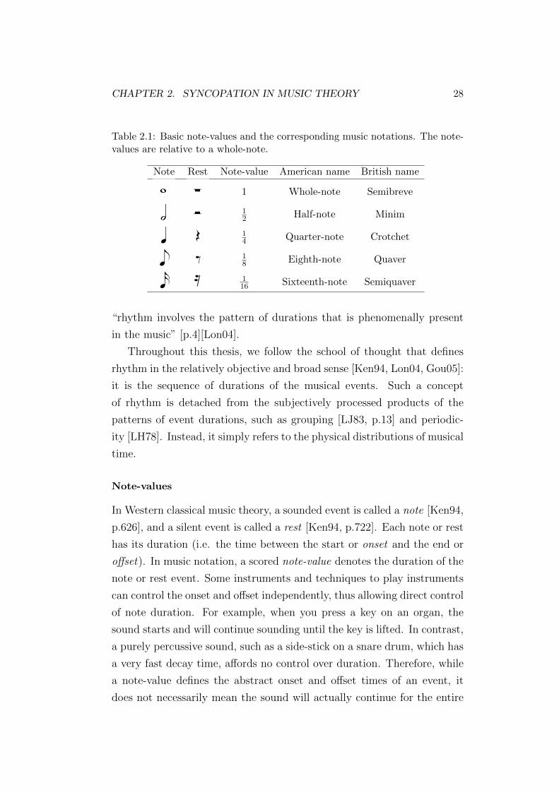
2.1 Basic note-values and the corresponding music notations.
The note-values are relative to a whole-note. . . . . . . . . 28
2.2 Comparisons of the properties of syncopation models. Ba-
sis: H - Hierarchical-based, C - Classification, O - Off-beat-
based, A - Autocorrelation-based. . . . . . . . . . . . . . . 44
6.1 Tempo (QPM) in relation to quarter-note time interval (ms).109
7.1 Linear regression coefficients for the BSC model. . . . . . . 135
7.2 Linear regression coefficients for the BSC2 model. . . . . . 136
7.3 Coefficients of the full models of multiple linear regression. 136
7.4 Coefficients of the reduced models of multiple linear regres-
sion. . . . . . . . . . . . . . . . . . . . . . . . . . . . . . . 138
13

List of Abbreviations
BPM Beats Per Minute
QPM Quarter-note Per Minute
TPM Tones-Per-Minute
SSL Short-short-long
s seconds
ms milliseconds
LHL Longuet-Higgins and Lee’s model
PRS Pressing’s model
TMC Toussaint’s Metric Complexity model
SG Sioros and Guedes’s model
TOB Toussaint’s Off-beatness model
WNBD Weighted Note-to-Beat Distance model
KTH Keith model
KSA Keller and Schubert’s Autocorrelation model
BSC Best-Single Combined model
WMC Weighted-Multiple Combined model
P&E Povel and Essens
14

Glossary of Symbols
∈ Set notation ‘in’ i.e. denotes membership of a set or se-
quence e.g. x ∈ X, x is a member of X.
∀ Set notation ‘For all...’
∃ Set notation ‘There exists...’
∅ The empty sequence.
〈·〉 Contents of angle brackets form a sequence.
∗ Concatenation operator for two sequences.⊙Iterative concatenation operator for sequences.
| · | Cardinality (length) of a sequence.
d·e Ceiling function (round up to nearest integer).
torg Time origin for a rhythm pattern.
tend End time of a rhythm pattern.
tspan Total duration for a rhythm pattern time-span.
ts Onset time of a note with respect to torg.
td Duration of note.
ν Dynamic or velocity of a note.
Y A sequence of notes yn.
T Time-span sequence, time points tm
V A sequence of normalised velocity values vm.
B Binary sequence (each element bm = dvme)X A logic don’t care term; considered equal to both
1 and 0 when comparing binary values.
L The metric level (range 0 to Lmax).
W The sequence of metrical weights wL.
Λ The sequence of subdivisions λL.
HL The sequence of metrical weights hm for metrical level L
that corresponds to the time points in T .
Ψ The sequence of terminal nodes ψi.
15
16
SM(Y ) Syncopation prediction for Y for model M
η Node type, i.e. note N or rest R.
κ Function used to calculate the sequence of terminal nodes
in the LHL model.
g Function to classify prototypes in the PRS model.
q Normalisation function in the PRS model.
f Recursive accumulation function in the PRS model.
ϕ Metricity of a rhythm-pattern in the TMC model.
ϑ Function that calculates difference level factor for the SG
model.
β Weighting factor used in function ϑ.
ρ, % Functions that calculate the next and previous indices of
notes in the SG model.
u Function that calculates the average of the difference be-
tween a note and its neighbours in the SG model.
γ Weighting factor used in function u.
sm Syncopation value of a note in the SG model.
φm Syncopation potential in the SG model.
cn The highest power of two no greater than a note’s duration
in the KTH model.
o, e Functions that classify whether a note starts and/or ends
off-beat in the KTH model.
kn Syncopation value for a note yn in KTH model.
ςm Off-beatness of a note in the TOB model.
W(yn) WNBD measure for a note yn.
d(·, ·) Distance function.
T (yn) Distance of a note yn to its closest beat.
µi A beat position in the WNBD model.
Υ Tempo (QPM).
M∼T Tempo-dependent version of model M.
SM∼T(Y,Υ) Syncopation prediction for Y played at tempo Υ for model
M∼T.
F Tempo-dependent scaling function.

Chapter 1
Introduction
Music is a temporal phenomenon; it unfolds over time. Rhythm describes
how musical events are structured in time. A key feature of musical
rhythm is regularity; periodicities in rhythms are perceived by human
listeners as beats. We naturally infer structure, known as meter, from
these underlying periodicities. Meter allows us to anticipate future events
and to engage with music, for example by dancing in time to the music.
Deliberate violations of meter in music can provide a curious, often disori-
enting sensation known as syncopation, and can occur with even a single,
carefully placed note in an otherwise regular stream. Hence, syncopation
provides a channel through which we may investigate the broader nature
of meter.
Syncopation is widely used in music and is even a central feature of
many music styles and cultures such as Jazz, Cuban Son and African
drumming. Various compositional techniques have been established to
achieve an effect of syncopation, but essentially they all undermine the
perception of meter by adding conflicting components onto the rhythm
surface. Syncopation can enhance the complexity and richness of rhythm;
it subtly teases our expectations and provides a mechanism to counter the
orderly nature of music. In this thesis, we explore the factors that give
rise to the perception of syncopation and test how well the established
theories of syncopation can explain our observations.
17

CHAPTER 1. INTRODUCTION 18
1.1 Motivations
The need for syncopation measurement
Syncopation is one of the fundamental rhythmic features in music and a
crucial aspect of character in many music styles and cultures. Having a
more complete understanding of syncopation and comprehensive models to
capture syncopation perception allows us to better understand the broad
aspects of music perception.
For example, the link between syncopation and beat or meter per-
ception has been widely investigated [HO81, SK01, KR01, TS03, FR07].
Multiple approaches to modelling the way that meter is perceived and
encoded from syncopated rhythm-context have been proposed [LHL84,
PE85, Par94, Eck01, VL11]. It has been found that syncopation has an
effect on rhythm identification [Moe12] and rhythm memorisation [FR07].
In addition to rhythm perception, the phenomenon of syncopation is
also linked to more elusive and subjective feelings and responses to music.
For example, one of the recent topics of debate explores whether syn-
copation facilitates or inhibits groove. Groove refers to the sensation of
wanting to move some part of the body to music [Mad06]. Some evidence
has suggested that adding syncopation led to stronger groove [MSD+13],
whereas some evidence has suggested their relationship is inverted-U-
shaped where the sensation of groove and pleasure is optimised at medium
syncopation, but decreased towards the extreme ends of degree of synco-
pation [WCW+14]. More than that, syncopation seems to affect human
emotion [KS11, Hur06] and some physiological responses, e.g. increased
heart rate [Slo91].
With the development of brain sciences in recent years, there has been
a growing interest in collecting neuroscientific evidence from both humans
and animals when listening to music. One particular focus is in what kinds
of neurophysiological responses are elicited by syncopation and how they
correlate with the sensations that syncopation arouses [MFD+01, LH09,
HLHW09, TK03, VOP+09]. For example, some evidence suggest that
syncopation elicits brain activity associated with violating sensory expec-
tations, and this effect is found from both adult listeners and newborn

CHAPTER 1. INTRODUCTION 19
infants which support the view that beat perception is innate [WHL+09,
HLHW09]. There is also evidence suggesting the link between meter in-
terpretation in a polymetric context and the activation of language ar-
eas [VWOR11]. These studies complement our understanding of the brain
mechanisms and functions in processing rhythm.
In the field of music information retrieval, syncopation has been consid-
ered a contributory feature in the computation of rhythm similarities be-
tween rhythm-patterns [Smi10, PRBH14, PT11]. Psychological evidence
has supported the relationship between syncopation and the perceptual
judgement of rhythmic similarities [Lad09, Str06, SH93]. Some evidence
has suggested that by involving perceptual features, instead of merely
building upon lower-level rhythmic features, the computation of rhythm
similarity improves the performance of rhythm classification tasks [GDPW04].
Thus a measure that captures perceptual syncopation will directly ben-
efit the development of algorithms for estimating rhythm similarity and
general rhythmic description.
In brief, syncopation interacts with a range of musical concepts and has
broad effects on music perception and cognition. Investigations on these
effects of syncopation need quantitative measures of syncopation that can
correctly reflect human perception. This provides the major motivation
for us to closely examine the existing theory and models for syncopation.
Lack of direct investigation on syncopation perception
It is clear that there is a need for a reliable, validated measure of synco-
pation. However, current approaches have either been based on indirect
perceptual measures or theoretical models that have not been formally
tested. As Figure 1.1 shows, studies that investigate the link between
syncopation and broad music perception and cognition rely on measures
of rhythm-complexity or predictions of syncopation by theoretical models,
i.e. links A - C in the figure.
For example, Fitch and Rosenfeld [FR07] controlled the degree of syn-
copation quantified by Longuet-Higgins and Lee’s syncopation model [LHL84]

CHAPTER 1. INTRODUCTION 20
Rhythm
Models of rhythm-complexity
Models of syncopation
Perceptual rhythm-complexity
Perceptualsyncopation
? ?
Music Perception
?
Beat Induction
Meter Perception
Emotion
Groove
Rhythm
Identification
Performance RhythmMemorisation
A
B
C
D
F G
E
Figure 1.1: Tested and untested relationships between theory and perception.Music perception studies have been utilising indirect measures of syncopationsuch as rhythm-complexity, or theoretical models of rhythm-complexity andsyncopation (indicated by links A - C). These models have only been testedagainst perceptual datasets of rhythm-complexity (links D and E). However,the relationship between syncopation perception and rhythm (link F) is stillunknown. A perceptual dataset for syncopation would be valuable for the eval-uation of theoretical models of syncopation and the linkage to music perceptionand cognition in general (link G).
(which will be discussed in detail in Sections 2.3 and 3.2.1) to test beat in-
duction, rhythm reproduction and rhythm memorisation. Likewise, Witek
et al. [WCW+14] tested the relationship between groove and predictions
of syncopation generated by Longuet-Higgins and Lee’s model. Similarly,
Keller and Schubert designed a model which they then used in experiments
to test the effect of syncopation on emotional responses [KS11].
There has been no attempt yet to directly measure syncopation per-
ception (Figure 1.1, link F). However, such an investigation is required in
order to allow a formal and systematic evaluation of the theory and mod-
els (link G). It is therefore questionable whether current music theory or
models can accurately predict the strength of syncopation as how human
listeners perceive it.
The concept of syncopation has often been fused with rhythm-complexity
(Figure 1.1, Links D and E) [Tou02, Thu08, SG11, Pre97, WCW+14], re-
sulting in ambiguities in the modelling of both percepts. As illustrated

CHAPTER 1. INTRODUCTION 21
in Figure 1.1, syncopation models have previously only been evaluated
against datasets of rhythm-complexity [GTT07, Thu08, SH07], such as the
perceptual dataset collected by Shmulevich and Povel [SP00] that com-
prises perceptual ratings of rhythm-complexity for 35 rhythm-patterns.
In summary, diverse theories and modelling approaches for syncopa-
tion have been heavily used in studies in multiple disciplines, yet, they
have not been proven to be entirely reliable so far. A direct investigation
of syncopation perception is therefore needed to test how well the theo-
ries and models capture perception, and to clarify the confusion between
syncopation and rhythm-complexity.
1.2 Methodology
To address the missing information on direct syncopation, we will use ap-
proaches from psychophysics to collect human data on syncopation per-
ception. Psychophysics applies psychological methods to quantify the re-
lationship between perception and stimulus [Ste75]. A fundamental postu-
late of psychophysics is that perception should have underlying objective,
physical correlates which may be quantified as features of the stimulus.
For example, intensity is the objective correlate of loudness (i.e. perceived
intensity).
The music score is a symbolic encoding that describes the set of events
comprising a piece of music. For the purposees of this thesis, we will deal
only with scores that describe Western common practice art music. Before
these notated events can be perceived as music by a listener, they must be
rendered (e.g. by the performer) as an acoustic pressure signal that varies
over time (Figure 1.2). The rendering process mediates the transformation
between the score and the perception. By manipulating the score, we can
find out what features of the score correspond to features of perception.
Main method and rationale
To directly investigate the perception of syncopation, we asked musicians
to provide ratings on a limited scale to indicate the perceived strength

CHAPTER 1. INTRODUCTION 22
Notated
Score
Musical
Performance
Listener
Perception
Figure 1.2: Transformation: from the music score to perception. Before thenotes on the score can be perceived as music by the listener, the score mustbe rendered (e.g. by a performer) as an acoustic (pressure) signal which variesover time.
of syncopation elicited by designed rhythm-stimuli. This method is suit-
able for the purpose because the most direct method to identify human
perception is by letting them describe what they have perceived (assum-
ing it can be explicitly and accurately described). Other methods, such
as measuring objective biophysical responses and behaviour, effectively
separate sensation and verbalisation and are therefore viewed as indirect
methods [BZ06].
In addition, we believe that scaled rating is the optimal approach to
collect subjective measures for our task. It is easy to implement and
provides well-specified and unified descriptors [BZ06]. It also allows quan-
tifiable subjective descriptions, which suits the concept of syncopation. In
contrast to other methods, such as quantifying the difference in syncopa-
tion between a pair of stimuli or ranking multiple stimuli by the degree of
syncopation, scaled rating does not require comparisons between stimuli
thus is simple for the listeners.
In contrast, previous studies adopted indirect methods that focus on
the objective measures, such as the difficulty in rhythm reproduction [PE85,
FR07], quality of rhythm recognition [FR07, Moe12], the consistency of
beat synchronisation [PE85, FR07] and brain activities [HLHW09, LH09].
These methods are based on the assumed relationship between perceived
syncopation and the indirect measure, but this assumption has not been
verified yet.

CHAPTER 1. INTRODUCTION 23
Experiment subjects
We selected musicians for our experiments. All of the participants had
several years of music training and experience, and thus they all under-
stand syncopation and felt confident about their perceptual ratings. Non-
musicians may not have been suitable for the task because there is no
guarantee that they are familiar with the concept of syncopation in the
same way as musicians would be.
Another reason to choose musicians is that some evidence suggest non-
musicians have a weaker ability to synchronise to the beats and organise
metrical structure than musicians [CPZ08, RD07, PK90]. Hence they may
be less sensitive to the perception of syncopation, because the sensation of
syncopation is built upon a firm grip on mental representations of meter.
General design of experiments
We conducted two experiments that involved collecting musicians’ ratings
on perceived syncopation. Experiment 1 focused on manipulation of the
rhythm-score as the objective correlate of perceived syncopation. In par-
ticular, we focused on testing the effect of location and distribution of
notes on syncopation. We used a monophonic, unaccented, and percus-
sive sound in creating rhythm-stimuli, in order to rule out the potential
confounding effects, such as dynamic, melodic and duration factors. A
metronome was played simultaneously with rhythm-patterns to experi-
mentally control the metrical interpretation [PE85]. Method and results
will be discussed in more detail in Chapter 4.
In Experiment 2, we selected a set of syncopated rhythm-patterns from
Experiment 1. These were played at different tempi (Section 2.1.4) to test
the relationship between tempo and perceived syncopation. The method
and results of this experiment will be discussed in Chapter 6.
In summary, we asked musicians to rate the degree of syncopation they
perceived in response to a rendering of each rhythm-stimulus. This serves
to directly investigate the perception of syncopation in a way that has not
been achieved by previous approaches. It is worth mentioning here that a
track of metronome is added into the rhythm-patterns to provide explicit

CHAPTER 1. INTRODUCTION 24
cues to the meter. This is a unique feature that differentiates our work
from previous approaches [PE85, SP00, FR07].
1.3 Goals and objectives
In this thesis, we address the following two main research questions:
• Research Question 1: What are the factors in rhythm influencing on
perceived syncopation?
• Research Question 2: To what extent do current theoretical models
of syncopation and music theory in general capture the perception,
and what elements are missing?
To find answers to these questions, our main objectives are:
• To conduct experiments that investigate the contributing factors to
perceived syncopation. In particular, the rhythmic attributes that
we target are: rhythm-components (i.e. micro units to form rhythm-
patterns), the combinations of different rhythm-components, time-
signature1 and tempo.
• To review and clarify the existing theory and models of syncopation.
• To evaluate syncopation models against human perceptual data.
1.4 Thesis outline
The main purpose of this thesis is to provide a step towards unifying
music theory with music perception in terms of syncopation. Figure 1.3
shows the overall arrangement of contents and the connections between
chapters. Chapters 2 and 3 explore the theory and models of syncopation.
Chapter 4 presents Experiment 1, which enables the formal evaluation
of the models in Chapter 5. Chapter 6 presents Experiment 2, which,
combined with findings in covered in Chapter 5, leads to the improvement
1In this thesis, we limit the tested time-signatures to isochronous 4/4 and 6/8 (see Sec-tion 2.1.3 for more details), and exclude non-isochronous (NI) meters [Lon04]

CHAPTER 1. INTRODUCTION 25
Figure 1.3: Thesis outline.
of the modelling of syncopation in Chapter 7. The following sections
provide a brief overview of the individual chapters.
Chapter 2
In this chapter, we start with presenting fundamental rhythmic concepts
that are directly relevant to the understanding of this thesis, including
rhythm, beat, meter and tempo. We then review how syncopation is
explained in music theory and summarise the main streams of thought in
the literature. Finally, we give a brief overview of the existing syncopation
models and categorise them by theoretical basis.
Chapter 3
This chapter provides a comprehensive review of syncopation models and
introduces a consolidated mathematical notation that unifies the field.
We first introduce some general mathematical terms and operations for
representing rhythm and meter. We then describe the mechanism of each
syncopation model with mathematical notations and illustrative examples.
Chapter 4
In this chapter, we address Research Question 1 by conducting an experi-
ment, which will be referred to as Experiment 1. This experiment involved
manipulating rhythm-patterns by choosing different rhythm-components
and time-signatures to produce audio stimuli. Using this stimuli, we col-
lected the subjective ratings of perceived syncopation for each stimulus.

CHAPTER 1. INTRODUCTION 26
Chapter 5
In this chapter, we address Research Question 2 by implementing the first
formal and direct evaluation of the models described in Chapter 3 using
perceptual data established from Experiment 1. Based on the evaluation
results, the strengths and weaknesses of the various theoretical approaches
are then identified.
Chapter 6
In this chapter, we further investigate Research Question 1 to test if syn-
copation is tempo-dependent. We present Experiment 2, in which we col-
lected perceptual ratings of syncopation of same rhythm-pattern played
at different tempi. In the beginning of the chapter, we provide a thorough
review of relevant studies in the literature. We then introduce the method
for the experiment, analyse the results and finally seek connections be-
tween our observations and the findings of related studies.
Chapter 7
This chapter explores ways to improve the modelling of syncopation per-
ception. Building on the findings in Chapter 5, we consolidate the most
successful elements piecemeal into new combined models. In addition, we
incorporate the findings from Chapter 6 into the new models, attempting
to capture the tempo-dependent nature of syncopation.
Chapter 8
We conclude the thesis with a revision of the answers to the research
questions. We focus on the major findings from our perceptual studies
and the areas where current theory explains perception and where it falls
short. We also propose research topics for the further investigation on
syncopation perception.

Chapter 2
Syncopation in music theory
In this chapter, we review the fundamentals of rhythm, including the
notions of beat, meter and tempo. We then investigate different definitions
given for syncopation in music theory, and collect them into four major
hypotheses. We follow this with a brief introduction of eight syncopation
models from current literature, which we will cover in more detail in later
chapters.
2.1 Fundamentals of rhythm
In order to introduce the concept of syncopation in music theory, we need
to start with some musical terms that describe fundamental aspects of
rhythm.
2.1.1 Rhythm
The word rhythm has been loaded with multiple meanings, some of which
are only vaguely related to each other. Some refer to rhythm as the regular
recurring patterns in time that can be structured (i.e. close to meter)
or grouped [LH78, LHL84, LJ83]. Some view it as the organisations of
events with different perceptual emphasis, as Cooper and Meyer state:
“the way in which one or more unaccented beats are grouped in relation
to an accented one” [CM60, p.6]. Some propose definitions for rhythm
in a broader sense, for example, the Oxford Dictionary of Music defines
rhythm as “everything pertaining to the time aspect of music, as distinct
from the aspect of pitch” [Ken94, p.724]. Similarly, London states that
27
CHAPTER 2. SYNCOPATION IN MUSIC THEORY 28
Table 2.1: Basic note-values and the corresponding music notations. The note-values are relative to a whole-note.
Note Rest Note-value American name British name
! £1 Whole-note Semibreve
@ £ 12 Half-note Minim
A ) 14 Quarter-note Crotchet
$ * 18 Eighth-note Quaver
% + 116 Sixteenth-note Semiquaver
“rhythm involves the pattern of durations that is phenomenally present
in the music” [p.4][Lon04].
Throughout this thesis, we follow the school of thought that defines
rhythm in the relatively objective and broad sense [Ken94, Lon04, Gou05]:
it is the sequence of durations of the musical events. Such a concept
of rhythm is detached from the subjectively processed products of the
patterns of event durations, such as grouping [LJ83, p.13] and periodic-
ity [LH78]. Instead, it simply refers to the physical distributions of musical
time.
Note-values
In Western classical music theory, a sounded event is called a note [Ken94,
p.626], and a silent event is called a rest [Ken94, p.722]. Each note or rest
has its duration (i.e. the time between the start or onset and the end or
offset). In music notation, a scored note-value denotes the duration of the
note or rest event. Some instruments and techniques to play instruments
can control the onset and offset independently, thus allowing direct control
of note duration. For example, when you press a key on an organ, the
sound starts and will continue sounding until the key is lifted. In contrast,
a purely percussive sound, such as a side-stick on a snare drum, which has
a very fast decay time, affords no control over duration. Therefore, while
a note-value defines the abstract onset and offset times of an event, it
does not necessarily mean the sound will actually continue for the entire

CHAPTER 2. SYNCOPATION IN MUSIC THEORY 29
A A" = = A A A = A A AA AAA A
1
2
1
4
1
4= +
1
8
1
8= +
1
8
1
8++
1
16+1
16
1
16+1
16
1
16+1
16+1
16+ +
A
+1
16=
Figure 2.1: The equation of note-values. A half-note is equivalent in note-valueto two quarter-notes, four eighth-notes or eight sixteenth-notes. The curly tailsof two or more eighth-notes can be jointed together by a beam [Tay89, p.3]; twoor more sixteenth-notes can be joined together by two beams.
A A A A A A A=
yy" = $A =
y(a) (b) (c)
* $Figure 2.2: Examples of triplets. (a) Three triplet quarter-notes are of thesame length as a half-note. (b) Three triplet eighth-notes are equivalent to aquarter-note. (c) A triplet can be a group of notes and rests.
duration.
Table 2.1 lists a set of basic note-values commonly used in music nota-
tion. It should be noted that these note-values do not represent absolute
time durations (e.g. seconds). Instead, they are relative durations with
respect to the whole-note which is treated as the reference. For exam-
ple, a half-note has a note-value of 1/2, which is half the duration of a
whole-note.
Each note-value shown in Table 2.1 can be divided by two to give the
value on the row below (the sixteenth-note can be further divided in two,
giving a thirty-second) and so on. In terms of durations, these note-values
then form the relationship shown in Figure 2.1: a half-note is equivalent in
note-value to two quarter-notes, four eighth-notes or eight sixteenth-notes.
The note-values in Table 2.1 are all halved to produce the row below
but a note-value may also be divided by some values other than a power of
two. In this case, the desired subdivision needs to be specified explicitly.
For example, we commonly see a group of three equal-duration events
played in the time of two, and this is known as a triplet figure [Ken94,
p.901]. The notation convention for this is to add the number 3 above the
group of events to be played as a triplet (Figure 2.2).

CHAPTER 2. SYNCOPATION IN MUSIC THEORY 30
rA A AAA A A A @ ArrA
(a) (b)
Figure 2.3: Examples of tied notes. (a) The final sixteenth-note is tied tothe first eighth-note, which creates a single note with duration equivalent tothree sixteenths. (b) An eighth-note, a half-note and a quarter-note are all tiedtogether, forming a total duration of seven eighths.
rA A r$ %" " r= A = A rA $=
(a) (b) (c)
34
12
14
+38
14
18
+716
14
18
+116+= = =
Figure 2.4: Examples of dotted notes. (a) A dotted half-note is equivalent tojoining a half-note with a quarter-note (i.e. half of a half-note). (b) A dottedquarter-note is equivalent to an eighth-note tied to a quarter-note. (c) A double-dotted quarter-note is equivalent to a quarter-note tied to an eighth-note (halfof quarter-note), then further tied to a sixteenth-note (half of the precedingeighth-note).
Tied notes and dotted notes
In music notation, it is possible to indicate that separate musical notes
(with the same pitch) should be played as a single note, by connecting
them with a tie; the duration of this single note is equal to the sum of the
note-values of individual notes [Tay89, p.33]. To illustrate, in Figure 2.3a,
the curved line connecting the fourth sixteenth-note and the first eighth-
note is the tie. The tied-note can also be further tied to following notes
such as in Figure 2.3b.
Another notational method to extend a note-value is to add one or
more dots after a note or a rest. Each dot extends the duration by half of
the preceding note-value. Examples of dotted notes and their associated
durations are shown in Figure 2.4.

CHAPTER 2. SYNCOPATION IN MUSIC THEORY 31
2.1.2 Beat
Some musical events give rise to moments of perceptual emphasis in the
musical flow; these are known as accents [CM60, p.7]. Accents can arise
from the contrast between rest and note, a change in dynamics (e.g. soft
to loud), a contrast in duration, or a change in pitch, or from a mixture
of these.
Perceived accents serve as the cues for human listeners to extract an
underlying periodic pattern [LJ83, p.17]. This perceived regular pattern
is known as the beat1 [Tra07], or the pulse [CM60, p.3]. Like the ticking
of a clock, a series of beats are equally spaced in time2.
Tactus
The perception of beat arouses synchronised movements in the form of
tapping, nodding and dancing [Lon04, pp. 9 - 12]. There can be multiple
periodicities (forming multiple beat sequences) perceived from a given mu-
sical excerpt, but usually only one or two of which are primarily tracked by
listeners for synchronising (e.g. tapping or dancing). This beat sequence
is referred as the tactus [LJ83, p.21].
2.1.3 Meter
In some music cultures, particularly in western music, recurring patterns
underlying a sequence of beats are usually strongly perceived. For exam-
ple, when listening to marching music, we intuitively count the beats as
‘one-two-one-two’ or could be said to feel ‘strong-weak-strong-weak’. Like-
wise, when listening to waltz, the beats are naturally structured as ‘one-
two-three-one-two-three’ or ‘strong-weak-weak-strong-weak-weak’. In this
way, the beat groupings form higher levels of periodicity, giving rise to a
multi-level structure, known as meter [Lon04, p.17].
1In this thesis, we focus only on the case of isochronous beats, as Parncutt’s notion of alayer of pulsation [Par94]
2The time intervals between successive beats are theoretically identical, but this is notalways desirable in expressive musical performance where the interval may be varied by theperformer for musical effect.

CHAPTER 2. SYNCOPATION IN MUSIC THEORY 32
Beat 1 2 3 4 1 2 3 4 1 2 3 4
S W S W S W S W
Beat 1 2 1 2 1 2 1 2 1 2 1 2
S W S W S W S W
1 2 3 1 2 3 1 2 3 1 2 3
S W WS W S W S W W S W W S W W
S W S W
1 2 3 4 5 6 1 2 3 4 5 6
S W W S W W S W W S W W
(a) (b)
(c) (d)
Figure 2.5: Examples of beat groupings and the resulting beat salience. Thegrey box indicates the group, or bar. S and W refer to strong and weak. (a) Atwo-beat grouping. (b) A three-beat grouping. (c) A four-beat grouping. (d)A six-beat grouping.
Beat grouping and beat salience
Lerdahl and Jackendoff state that “fundamental to the idea of meter is the
notion of periodic alternation of strong and weak beats” [LJ83, p.19]. The
‘strong’ or ‘weak’ here describes the perceptual beat salience. Recalling
the examples of marching music and waltz, patterns of beat organisation
may be illustrated in dot notation as in Figure 2.5a-b. Here, the two-
or three-beat groupings form two levels of periodicities, and the first beat
marks the coincidence of these two periodicities. If the beat at a particular
level of periodicity also exists in the next larger level, it is called a strong-
beat, otherwise is a weak-beat.
Additionally, the non-prime beat groupings give rise to equal size sub-
groups of beats (i.e. the prime factors), hence forming multi-level metrical
structures. For example, the four-beat grouping in Figure 2.5c forms two
groups of two beats. Likewise, the six-beat grouping in Figure 2.5d forms
two groups of three beats. It is also possible to subdivide a group of six
into three groups of two beat, and this gives a metrical structure with
different rhythmic emphases. It should be noted that for meter to be well-
formed [LJ83, pp.69-72], we may only group elements that are of equal
length. For example, while a six-beat grouping can be two threes or three
twos, it cannot be divided into a group of two and a group of four.

CHAPTER 2. SYNCOPATION IN MUSIC THEORY 33
Figure 2.6: Duple versus triple, simple versus compound. Meter can be cate-gorised by patterns of beat grouping and beat subdivision. Two-beat group-ing and three-beat groupings are referred to as duple and triple respectively.Binary- and ternary-beat subdivisions are referred to as simple and compound.
Bar
When composing, particularly when notating music, composers will gen-
erally try to choose an appropriate primary beat grouping. This serves
as an indication to the performers of how to count beats, and thus how
to interpret the score. Each complete cycle of this primary beat grouping
is called a bar (or measure) and in musical notation is enclosed between
two bar lines [Ran86, p.506] (represented by the grey boxes in Figure 2.5).
The first beat in a bar is called the down-beat, corresponding to all the
beats labelled 1 in Figure 2.5.
Time-signature
A time-signature is used for notating meter in the musical score. It is
usually indicated by a fraction where the denominator indicates the basic
note-value counted in a bar, and the numerator indicates the number
of such note-values making up the bar [Ran86]. For example, a time-
signature of 2/4 means a bar consists of two units, each of which has
a note-value of 1/4, i.e. a quarter-note (Table 2.1). Similarly, a time-
signature of 6/8 means a bar comprises six units, each of which is an
eighth-note.
As shown in Figure 2.6, the basic types of beat grouping include two
beats per bar and three beats per bar. These groupings are referred to as
duple and triple respectively [Ran86, p.506]. Two types of beat subdivision
are also distinguished: simple refers to a binary beat subdivision, and

CHAPTER 2. SYNCOPATION IN MUSIC THEORY 34
Figure 2.7: Time-signatures and their hierarchical structures, patterns of beatgroupings and beat subdivisions. (a) A 2/4 time-signature. (b) A 4/4 time-signature. (c) A 3/4 time-signature. (d) A 6/8 time-signature.
compound refers to a ternary subdivision [Ran86, p.506].
Figure 2.7 presents four time-signatures commonly adopted in music
notation, in the form of a tree structure. The time-signature of 2/4 and
4/4 are counted as simple-duple meters3, because both feature two-beat
groupings and binary subdivisions. The time-signature of 3/4 features
a three-beat grouping and binary subdivision, therefore is known as a
simple-triple meter. In contrast, in 6/8 time, a two-beat grouping and
ternary-beat subdivision constitute a compound-duple meter.
There is a common misinterpretation that the denominator in the frac-
tion of time-signature refers to the note-value of the beat, and the numer-
ator indicates the number of beats. This may be true for simple meters,
but cannot work for compound meters [Lon04, p.18]. Take 6/8 for exam-
ple (Figure 2.7d), the beat level is carried by dotted notes with note-value
3/8, instead of the eighth-notes with note-value 1/8.
Metrical levels
So far, we have discussed the origin of meter, which manifests in the higher
levels of periodicities structured from the fundamental periodicities (i.e.
beats) in a rhythm sequence. We have also introduced concepts related to
3As a special case of duple meter, 4/4 is sometimes termed quadruple meter for its four-beatrecurrence.

CHAPTER 2. SYNCOPATION IN MUSIC THEORY 35
meter, including bar, time-signature, and categories of metrical structure
in terms of patterns of beat grouping and beat subdivision. But why do
we need to know these? What is meter for? Essentially, meter is used for
providing a framework to structure rhythm. Borrowing from London, the
relationship between rhythm and meter can be described thus: “meter is
a mode of attending, and rhythm is that to which it attend” [Lon04, p.4].
Earlier, in Figure 2.7, we employed tree diagrams to present the metri-
cal structure of different time-signatures. Throughout this thesis, we refer
to each (horizontal) layer in the tree as a metrical level, representing the
units in this level of periodicity. Each node in the tree is referred as a
metrical position.
Different rhythms in the same time-signature are fitted into in the
same framework of meter, but they may project different sets of metrical
levels. As shown in Figure 2.8, the three one-bar rhythm-patterns are
in a time-signature of 2/4 but have different number of metrical levels.
Defined by the time-signature, their bar levels all locate at the half-note
level, and all beat levels locate at the quarter-note level. However, the
lowest metrical level for the three rhythms are different, because it is
carried by the shortest note-values presented in the rhythm. This leads
to the concept of tatum, which is formally defined in [Bil93, p.22] as “the
regular time division that most highly coincides with all note onsets”4.
Therefore the tatum levels for three rhythms in Figure 2.8 are the a)
quarter-note level, b) eighth-note level and c) the sixteenth-note level.
Finally, tactus is the periodicity that human listeners naturally tap to or
dance to (Section 2.1.2). Which metrical level will be selected as tactus
depends on tempo. In the following section, we introduce the concept and
notation of tempo in music, and we will continue to review the relationship
between tactus and tempo in Chapter 6.
4It should be noted that there is not always a tatum solution for all types of music;hardanger fiddle music for example [Lon04]

CHAPTER 2. SYNCOPATION IN MUSIC THEORY 36
Figure 2.8: Metrical hierarchies projected by rhythm-patterns in a given time-signature. Metrical hierarchy is presented as a tree structure as in Figure 2.7.The bar level and beat level are determined by the time-signature, and areindicated in grey and pink respectively. The tatum level, indicated in green, isthe smallest metrical level. Any level could be selected as the tactus, indicatedin blue.
2.1.4 Tempo
Tempo describes the speed of a musical excerpt. Before the invention of
the metronome, composers would indicate the speed of a piece of music
using Italian musical terms (e.g. allegro means fast, quick and bright,
Moderato means moderately). These terms would be interpreted by the
musician in order to perform to piece. With the invention of metronome,
it became possible for composers to specify precisely what speed the music
should be played at by linking a note-value to a specific beat rate, with
a metronomic indication. This is defined as the rate per unit of time
of a given metrical level [Ran86, p.873]. Figure 2.9 shows an example
of tempo indication in beginning of a musical score. By convention in
musical notation, the tempo is indicated in beats per minute, where the
beat is defined by a certain note-value.
A number of concepts are closely linked to tempo in the perceptual
domain, such as the pulse rate that people would tap or dance to, called
the tactus rate (Section 2.1.2). It is also related to the notion of preferred
tempo (or indifference interval) that refers to the rate when music sounds
neither too fast nor too slow but just right [QW06, MJH+06, Fra63]. In

CHAPTER 2. SYNCOPATION IN MUSIC THEORY 37
aaaaaaaaa3 I¥ 120I A A A A A A A A
Figure 2.9: Example of tempo indication in the beginning of the musical score.The tempo of a music excerpt, shown here in red by the metronomic indication,is indicated to be 120 beats per minute (BPM), counting each quarter-note asa beat. Therefore, each quarter-note has a duration of 0.5 seconds.
this thesis, we will refer to tempo only as the defined beat rate in the music
notation (Figure 2.9), as opposed to the subjective judgement of tempo.
2.2 Definitions for syncopation
So far, we have introduced the concepts of beat and meter. From the com-
poser’s or performer’s perspective, they serve as the fundamental struc-
ture for various interesting rhythm-patterns to be built upon. From the
listener’s perspective, they are the underlying precepts extracted from the
temporal patterns in the music. Sometimes, however, composers or per-
formers may deliberately set up rhythm-patterns to undermine the estab-
lished meter structure, and create a situation where the meter may not be
readily perceived from the rhythm surface for listeners. This phenomenon
is known as syncopation.
The classic definition of syncopation is the “momentary contradiction
of the prevailing meter or pulse” [Ran86, p.861]. Music theorists have
attempted to explain the effect of syncopation using a range of prototypical
rhythm configurations. Thus, we see diverse opinions of the scopes of
syncopation in terms of rhythmic instances. In the following sections,
we are going to review the definitions and explanations of syncopation
in music theory, and try to classify the main schools of thought on the
subject.

CHAPTER 2. SYNCOPATION IN MUSIC THEORY 38
r
II(b) Tied-note on strong beat(a) Rest on strong beat - "loud rest"
HI
(c) Accent on weak beat and missing strong beat
GI
(d) Loud rest and accented weak beat
A A)S W W
A A AA A
S W S W
A A)S W W
A
S W S W
A " WA
S W
W W W W W W
Hi-hat
Side-stick
))
Kick
GI
-
- -
-
-
Figure 2.10: Examples of syncopation aroused from violation of regular beatsalience. (a) A rhythm-pattern that has rests (indicated in red) placed onthe down-beats (i.e. strong-beats). (b) The note on the second strong-beat(indicated in red) is tied to the previous note, causing an absence on the down-beat. (c) The rhythm-pattern contains an onset and agogic (durational) accenton the second weak-beat, and absence of note on the following strong-beat. (d)The reggae drum-pattern in “Stir It Up” by Bob Marley. It is also a mixtureof missing down-beat and accented weak-beat.
2.2.1 Violation of the regular beat salience
A metrical structure is inbuilt with allocations of metrical weight (strong
or weak) at each beat position (see Section 2.1.3). All explanations of syn-
copation share the consensus that it involves the violation of the regular
succession of strong- and weak-beats, by creating an absence of sounded
note on the strong-beats, and/or by shifting accents to notes on the weak-
beats (Figure 2.10 provides some rhythm examples to demonstrate these
two effects). The majority of sources refer syncopation to both occa-
sions [Ran86, Ken94, Hur06, LHL84, HO06, Tem99, Tem01], with the
exception of Cooper and Meyer who exclude the occasion of accented
weak-beats from the scope of syncopation [CM60, p.100].
Huron [Hur06, pp. 295-297] specifies five types of syncopation af-
fected by accenting weak-beats in different ways (see Section 2.1.2). These
are: onset syncopation (due to note/rest positions), dynamic syncopation
(sounding notes loudly on weak-beats), agogic syncopation (placing longer

CHAPTER 2. SYNCOPATION IN MUSIC THEORY 39
r
II(a) Off-beat notes followed by a rest on the next beat
*
A A
$
A
* $ * A AA A* $A A
II A r r$ A$ A A A A A
(b) On-beat notes tied to the previous off-beat notes
Figure 2.11: Examples of off-beat notes that followed by a rest or a tied-note onthe next beat. Two short pieces of rhythm in 4/4 are presented. The grey dotsindicate the beat location. In (a), there are four notes (in red) enter betweenthe beats and the following beat is placed with a rest note. In (b), two notesoccur off-beat and are tied by the notes on the following beat. Both are thoughtto arise syncopation [CM60, LHL84, HO06].
notes on weak-beats), harmonic syncopation (changes in pitch/harmony
on weak-beats) or mixed syncopation (a combination of the above).
2.2.2 Off-beat
When a note is placed on the beat, it is called on-beat ; otherwise it is
off-beat. Off-beat events are thought to cause a shift of the emphasis away
from the strong-beats, hence producing syncopation. However, theories
diverge here where some state that only an off-beat event followed by an
unfilled beat gives rise to syncopation, while some do not.
Cooper and Meyer were exponents of the idea that syncopation is
aroused from shifting the note on the beat backward in time (i.e. move
it to be earlier). They defined syncopation as “a tone which enters where
there is no pulse on the primary metric level (the level on which beats are
counted and felt) and where the following beat on the primary metric level
is either absent (a rest) or suppressed (tied)” [CM60, p.100]. Examples
are shown in Figure 2.11. Longuet-Higgins and Lee [LHL84] expressed the
same notion, which was then formalised in their mathematical model, the
mechanisms for which will be further discussed in Section 3.2.1.

CHAPTER 2. SYNCOPATION IN MUSIC THEORY 40
II(a)
A A$ A A $A A II A$ $(b)
A II A
(c)
Figure 2.12: Syncopation types as defined in [Kei91]. Grey dots indicate beats.(a) presents hesitation, where a note (in red) ends off-beat; (b) presents antic-ipation, where the note starts off-beat; and (c) presents syncopation, where itboth starts and ends off-beat.
In contrast, some believed that an off-beat event would result in syn-
copation regardless of the rhythmic context it is in. For instance, Keith
stated that “syncopation occurs when events start or end off the beat” [Kei91],
specifying three types of syncopated event, named hesitation, anticipation
and syncopation (examples of which are shown in Figure 2.12). The de-
gree of syncopation is differentiated by the rhythmic context in which
the off-beat event is placed, and is thought to increase from hesitation to
anticipation then to syncopation. Nevertheless, they are all regarded as
manifestation of syncopation, whereas hesitation is not defined as a form
of syncopation by other theorists [CM60, LHL84].
A similar notion can be found in [Tou05, GMRT05], where capturing
off-beat events is the major focus in the modelling of syncopation. Gomez
et. al [GMRT05] posit that the sense of syncopation is aroused by the
effect of imbalance, and that this is a result of lopsided placing of the off-
beat events. The essence of their syncopation model, the Weighted Note-
to-Beat Distance model, is that the strength of syncopation is inversely
related to the distance of each note to its nearest beat, i.e. the closer the
note is to the beat, while it is still off-beat, the higher syncopation it gets.
2.2.3 Transformation of meter
Some theories state that syncopation can be aroused by a sudden trans-
formation of the fundamental character of the meter [Ran86, Ken94]. For
example, a change of feel from duple to triple, as affected by alteration
of accents in the rhythm (Figure 2.13a) or a change of time-signature in
the score (Figure 2.13b). The transformation of meter can give rise to

CHAPTER 2. SYNCOPATION IN MUSIC THEORY 41
(a)
HI GIKM A A AA A A A A A A A A> > > > >A A A A A A> > > A A A A A AA A A A A A A AA A AA
(b)
Figure 2.13: Examples of transformation of meter.
the effect of shifting the bar line, and may cause one of the weak-beats to
function as a strong-beat [Ran86].
2.2.4 Polyrhythm
A large set of rhythms that result in a sense of competing meters is
polyrhythms (or cross-rhythms). Polyrhythm has been defined as “the
simultaneous use of two or more rhythms that are not readily perceived
as deriving from one another or as simple manifestations of the same me-
ter” [Ran86, p.669]. A common use of polyrhythm in composition is a
triplet over a binary subdivision of the beat, e.g. Figure 2.14a. This type
of polyrhythm is often referred as 3:2 polyrhythm or hemiola5 [Ken94,
p.398]. Another example is 4:3 polyrhythm, shown in Figure 2.14b, where
the periodicities of four events (from the eighth-notes) and three (from
the triplet) cannot resolve to a single grouping of events. Krebs [Kre99]
described this phenomenon as metric dissonance, aroused by conflicting
periodicities.
From the perspective of meter, polyrhythms present the situation where
two (or more) different metrical hierarchies have to co-exist at the same
time. In other words, one metrical hierarchy that is only allowed a single
type of subdivision at each level cannot capture the conflicted groupings
in a polyrhythm. For example, in Figure 2.14a, the rhythm-pattern on
the top line suggests that the bar should be equally subdivided into three
(i.e. three groups of two eighth-note beats), whereas the bottom line sug-
gests a subdivision of the bar by two (i.e. two groups of three eighth-note
beats). These two different groupings of eighth-note in the bar cannot be
resolved into one metrical hierarchy. Similarly, in Figure 2.14b, the tree
5More specifically, this is known as vertical hemiola. The alternative, horizontal hemiola,refers to the transformation from duple to triple [Ran86, p.389], e.g. Figure 2.13a.

CHAPTER 2. SYNCOPATION IN MUSIC THEORY 42
(a)
GI
A AA A
y
A
KM
A A AA A
(b)
A A
A A A A A
" "
A A AA A
"y
$ $$ $
Top Line Bottom LineTop Line Bottom Line
"
Figure 2.14: Examples of polyrhythms and the resulting competing metricalhierarchies. (a) A 3:2 polyrhythm (often referred to as a hemiola). (b) A 4:3polyrhythm.
structure of the eighth-notes rhythm-pattern on the top line fits the met-
rical hierarchy implied by the scored time-signature 2/4 (two groups of
two). However, the triplet pattern on the second line suggests a separate
hierarchy with a subdivision of three that cannot fit with groupings of
four.
In the literature, there appears to be no clean cut between syncopation
and polyrhythm. Many theorists do not treat polyrhythm as a form of syn-
copation [Ran86, Ken94, LHL84, Lon04, CM60, HO06, Pre97], while some
think polyrhythms strongly challenge metric construals, therefore feature
syncopation [HO81, GMRT05]. London [Lon04] described polyrhythm
as a “full-blown metric ambiguity”, whereas syncopation was a “short-
term mismatch” between meter and rhythm. Indeed, compared to the ef-
fects aroused by emphasising weak-beats over strong-beats or by a sudden
change of time-signature, polyrhythms produce a more constant mismatch
between rhythm and meter; this seems to violate the widespread notion
that the effect of syncopation is “momentary” [Ran86]. We have chosen
to follow the broader interpretation of syncpation ( i.e. that it includes
polyrhythms), in our experiment design in Chapter 4.

CHAPTER 2. SYNCOPATION IN MUSIC THEORY 43
MODELS
Hierarchical Off-beatClassification Autocorrelation
TIMELINE
1984
1991
1997
2002
2005
2011
LHL
KTH
PRS
TMC
SG
TOB WNBD
KSA
Figure 2.15: Models used for predicting syncopation, which are categorised bytheoretical basis and main methodolgy.
2.3 Overview of syncopation models
Ambiguity in the definition of syncopation has led to a number of differ-
ent models [LHL84, GMRT05, SG11, Tou05, Kei91, KS11], representing
multiple competing hypotheses. Additionally, models of rhythm complex-
ity [Pre97, Tou02] have also been applied to syncopation prediction in
a number of previous studies in the literature [GTT07, Thu08] and as a
result we include them in this thesis as well.
2.3.1 Categories of models
Figure 2.15 presents the models in categories for syncopation and the
development of these models tracing back to 1984. In general, hypotheses
for these syncopation models fall into four broad categories: hierarchical,
off-beat, classification and autocorrelation.

CHAPTER 2. SYNCOPATION IN MUSIC THEORY 44
Hierarchical models are designed to capture the violation of the regular
succession of beat salience or metrical weights (Section 2.2.1 and 2.2.2).
Four models fall into this category: Longuet-Higgins and Lee’s model
(LHL) [LHL84], Pressing’s model (PRS) [Pre97], Toussaint’s Metric Com-
plexity model (TMC) [Tou02] and Sioros and Guedes’s model (SG) [SG11]
that is developed from TMC.
Another approach is to classify individual notes or rhythm sequences
into a number of pre-determined syncopation types. We will refer to
this category of modelling hypothesis as classification models. Keith’s
model [Kei91] (KTH) and the PRS model adopted this approach.
Off-beat models ignore metrical hierarchy and instead attempt to cap-
ture note onsets that fall in between strong-beat positions (Section 2.2.2).
Two models fall into this category: Gomez et al.’s Weighted Note-to-
Beat Distance (WNBD) [GMRT05] and Toussaint’s off-beatness measure
(TOB) [Tou05].
Finally, Keller and Schubert’s autocorrelation-based model [KS11] (KSA)
differs from the other categories, and we refer to this approach as an auto-
correlation model. This model measures the accent strength (the sum of
durational and melodic accents weights [Dix01, MPF09, Par94, Tho82]) of
each musical event in a rhythmic sequence, then calculates the two-beat-
autocorrelation coefficients. The hypothesis is that the more different
events separated by two beats are in terms of accent strength, the greater
the violation of metric structure is, hence resulting in higher syncopation.
2.3.2 Capabilities of models
The various models for syncopation represent different hypotheses in terms
of rhythmic features that contribute to syncopation and therefore possess
different capabilities in the modelling. Table 2.2 summarises the eight
models in terms of category and the musical features that they can capture.
All the models use temporal features (i.e. onset time point and/or
note duration) in the modelling. The SG model also process dynamic
information of musical events in rhythms (i.e. dynamic accents), and the
KSAmodel takes account of temporal, dynamic and melodic information

CHAPTER 2. SYNCOPATION IN MUSIC THEORY 45
Table 2.2: Comparisons of the properties of syncopation models. Basis: H -Hierarchical-based, C - Classification, O - Off-beat-based, A - Autocorrelation-based.
Model Basis Onset Duration Dynamics Melody Mono Poly Duple TripleLHL H X X X XKTH C X X X X XPRS H,C X X X XTMC H X X X XTOB O X X X X X
WNBD O X X X X X XSG H X X X X X
KSA A X X X X X
of musical events.
In this thesis, we will use the term monorhythm to refer to any rhythm-
pattern that is not polyrhythmic. All the models can measure syncopation
of monorhythms, but only the KTH, TOB and WNBD models can deal
with polyrhythms.
Finally, all the models can deal with rhythms (notated) in a duple
meter, but only six models can cope with rhythms in a triple meter. They
are the LHL, PRS, TMC, TOB, WNBD and KSA models.
2.4 Summary
In this chapter, we have reviewed the theoretical underpinnings of rhythm
and introduced the definitions for syncopation and how it is explained in
the music theory literature. We have explained the note-values that are
used in western music notations, and demonstrated the construction of
rhythm-patterns from combinations of notes and rests with various note-
values. We have also discussed the concepts of beat, meter, and tempo.
Based on these fundamental elements of rhythm, we have outlined four
main schools of thought on the manifestation of syncopation, and intro-
duced eight theoretical models of syncopation from literature to provide
a broad picture of the state of the art.

Chapter 3
Review of syncopation models
In this chapter, we take a step further in reviewing the models of syncopa-
tion. In order to provide an explicit representation of the models, we con-
solidate the notations into mathematical equations, and walk through ex-
amples to assist readers in understanding the mechanisms of these models.
By doing this, we benefit from unambiguous explanations of the models
(as opposed to describing models in prose), and a smoother step towards
programming codes of models implementation.
In the chapter, we introduce and define some relevant mathematical
terms and operations. Then, we apply these mathematical notations in
formalising some rhythmic concepts we mentioned in Chapter 2. Finally,
we review each of the seven well-known syncopation models in depth by
providing unified representation of mathematical equations.
3.1 Background
In order to review the models in detail, we will first define some general
mathematical terms and operations with which we will represent rhythm
and meter. A key to the set notation symbols we use can be found in the
Glossary of Symbols.
3.1.1 Sequences
We use the term sequence to refer to a finite, ordered set that may con-
tain duplicated elements. A sequence Q of individual elements qn will be
46
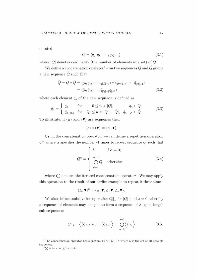
CHAPTER 3. REVIEW OF SYNCOPATION MODELS 47
notated
Q = 〈q0, q1, · · · , q|Q|−1〉 (3.1)
where |Q| denotes cardinality (the number of elements in a set) of Q.
We define a concatenation operator1 ∗ on two sequencesQ and Q giving
a new sequence Q such that
Q = Q ∗ Q = 〈q0, q1, · · · , q|Q|−1〉 ∗ 〈q0, q1, · · · , q|Q|−1〉
= 〈q0, q1, · · · , q|Q|+|Q|−1〉 (3.2)
where each element qn of the new sequence is defined as
qn =
{qn for 0 ≤ n < |Q|, qn ∈ Q;
qn−|Q| for |Q| ≤ n < |Q|+ |Q|, qn−|Q| ∈ Q.(3.3)
To illustrate, if 〈M〉 and 〈H〉 are sequences then
〈M〉 ∗ 〈H〉 = 〈M,H〉.
Using the concatenation operator, we can define a repetition operation
Qα where α specifies the number of times to repeat sequence Q such that
Qα =
∅, if α = 0;
α−1⊙a=0
Q, otherwise.(3.4)
where⊙
denotes the iterated concatenation operator2. We may apply
this operation to the result of our earlier example to repeat it three times:
〈M,H〉3 = 〈M,H,M,H,M,H〉.
We also define a subdivision operation Q‖λ for |Q| mod λ = 0, whereby
a sequence of elements may be split to form a sequence of λ equal-length
sub-sequences:
Q‖λ =⟨〈·〉0, 〈·〉1, ..., 〈·〉λ−1
⟩=
λ−1⊙a=0
⟨〈·〉a⟩
(3.5)
1The concatenation operator has signature ∗ : S× S→ S where S is the set of all possiblesequences.
2⊙ is to ∗ as∑
is to +.

CHAPTER 3. REVIEW OF SYNCOPATION MODELS 48
Figure 3.1: An example note sequence.
Two note events y0 and y1 occur in the time-span between time origin torg andend time tend. The time-span duration tspan is three quarter-note periods. Therests at the start and end of the bar are not explicitly represented as objects intheir own right here but as periods where no notes sound.
where the ath sub-sequence 〈·〉a takes the form
〈·〉a =
Θ−1⊙θ=0
〈qθ+aΘ〉 where Θ =|Q|λ
, qθ+aΘ ∈ Q. (3.6)
As an example, we may subdivide our repeated example from above into
two sub-sequences
〈M,H,M,H,M,H〉‖2 =⟨〈M,H,M〉, 〈H,M,H〉
⟩.
3.1.2 Rhythm in continuous time
The term time-span has been defined as the period between two points
in time, including all time points in between [LJ83]. To represent a given
rhythm, we must specify the time-span within which it occurs by defining
a reference time origin torg and end time tend, the total duration tspan of
which is
tspan = tend − torg (3.7)
A single, note event y occurring in this time-span may be described
by the tuple (ts, td, ν) as shown in Figure 3.1, where ts represents start or
onset time relative to torg, td represents note duration in the same units
and ν represents the note velocity (i.e. the dynamic; how loud or accented
the event is relative to others) ,where ν ≥ 0.
This allows us to represent an arbitrary rhythm as a sequence of notes
Y , ordered in time
Y = 〈y0, y1, · · · , y|Y |−1〉. (3.8)

CHAPTER 3. REVIEW OF SYNCOPATION MODELS 49
We will use superscript notation to index individual elements of tuples so
ytsn for example will represent the onset time for the nth note in Y .
Rests, time periods where there is an absence of sounded notes in
music, are as important as the note events themselves. The representation
detailed here allows a rest to occur at the start of the rhythm where yts0 ≥ 0
i.e. the first note starts after torg, a rest may occur in between notes where
ytsn + ytdn < ytsn+1 and there may also be a rest at the end of the pattern
if the final note finishes sounding before the end of the time-span i.e.
yts|Y |−1 + ytd|Y |−1 ≤ tspan.
3.1.3 Discrete time representation
So far, ts and td have been considered to be continuous variables in time.
However, for the purposes of music theory it often serves to quantise them
such that they are given as integer multiples of some discrete time unit
∆t. Discretising time in this way, we may represent the time-span of Y
as a sequence T comprising |T | equally spaced time points:
T =
|T |−1⊙m=0
〈m∆t〉 = 〈t0, t1, · · · , t|T |−1〉. (3.9)
where
|T | = tspan
∆t. (3.10)
With the exception of Keith [Kei91], the syncopation models reviewed
here only take account of note onsets ignoring notated duration. We may
therefore choose ∆t (and thus |T |) for a given time-span sequence depen-
dent upon onset times of notes in Y ; the choice of value being arbitrary
provided that every note onset ytsn can be precisely expressed as an integer
multiple m∆t where m < |T |. For any particular sequence Y , there will
be a minimum-length time-span sequence Tmin for which
Tmin = arg minT
|T | (3.11)
where
T ∈ {T : ∀ yn ∈ Y, ∃ tm ∈ T : tm = ytsn } (3.12)

CHAPTER 3. REVIEW OF SYNCOPATION MODELS 50
Figure 3.2: Example rhythm-patterns with their minimum-length time-spanand velocity sequences. Each of the rhythm-patterns above is a single bar in4/4 meter and we will assume a tempo of 120 quarter-note BPM (i.e. 2 beatsper second). Example (a) contains four equally spaced quarter-notes with thefirst and third notes accented (refer to Section 2.1.2), so |Tmin| = 4 with ∆tof half a second. Example (b) contains both quarter-notes and quarter-notetriplets thus |Tmin| = 12 with ∆t = 1/6s and (c) the Son clave rhythm containsan onset in the fourth 16th note position so |Tmin| = 16 with ∆t = 1/8s.
i.e. Tmin is the shortest possible time-span sequence for which the start
time ytsn of every note in Y has a corresponding time point tm.
With the time resolution of T determined, we may represent the notes

CHAPTER 3. REVIEW OF SYNCOPATION MODELS 51
in Y as a sequence V of sampled velocity values
V =
|T |−1⊙m=0
〈vm〉 (3.13)
where
vm =
{yνn
max(yν :yν∈Y ), ∃yn ∈ Y : ytsn = m∆t;
0, otherwise.(3.14)
i.e. each element vm in V corresponds to the velocity at time point tm in
T . The value of vm is the normalised velocity yνn of a note in Y if an onset
is present at m∆t or zero where there is none. Figure 3.2 shows example
minimum-length time-span sequences for three one-bar rhythm-patterns
and their associated minimum-length velocity sequences. The rhythm-
pattern shown in Figure 3.2a is represented with Vmin = 〈1, 0.8, 1, 0.8〉. An
equally valid velocity sequence could be produced with values |T | = 8 and
∆t = 0.25s giving V = 〈1, 0, 0.8, 0, 1, 0, 0.8, 0〉, but every second element
is redundant in this case.
In Figure 3.2a, two notes are accented, therefore velocities in V vary
in magnitude (in our example, between arbitrary values of 0.8 or 1). In
some cases, we are concerned with whether a note onset is present at a
particular time point rather than what its velocity value is, so we will
introduce a binary sequence B of bits bm given by
B = 〈b0, b1, · · · , b|B|−1〉 =
|T |−1⊙m=0
⟨dvme
⟩, vm ∈ V (3.15)
where d·e denotes the ceiling function. Thus, for the rhythm-pattern in
Figure 3.2a B = 〈1, 1, 1, 1〉. In Figure 3.2b and c, no dynamics or accents
are shown, so all notes are assumed to be of the same velocity, thus B will
be equal to V .
A useful property of this binary sequence representation is that simple
combinational logic can be employed to analyse the matching of rhythm-
patterns by specifying masking sequences [Lew72].For example, a binary
sequence B with onsets in every position (as in Figure 3.2a) would be

CHAPTER 3. REVIEW OF SYNCOPATION MODELS 52
matched by the expression 〈1〉|B|; a sequence containing |B| ones. Like-
wise, a sequence with no onsets (i.e it contains only a rest) would be
equivalent to |B| zeros which may be written 〈0〉|B|. We may express a
mask pattern that contains a single onset at the very start of the time-
span followed by rests as 〈1〉 ∗ 〈0〉|B|−1. We also utilise the digital logic
notion of a don’t care notated as X. This type of value can be used in a
mask pattern to signify that both 1 and 0 can be matched in that position.
For example, if we want to match any rhythm-pattern that starts with a
rest, we could express this as the mask pattern 〈0〉∗〈X〉|B|−1 (the sequence
shown in Figure 3.2b would match this pattern).
3.1.4 Metrical hierarchy
The previous section defined the atomic representation of note events in
time. As listeners however, the way we perceive the grouping of those
events is of huge importance in the analysis of syncopation. An isolated
note event cannot be syncopated; for syncopation to exist, it is necessary
for the listener to have already developed a sense of meter. In Section 2.1.3,
we have introduced the concept of isochronous-meter from the perspec-
tive of music theory. The following sections formalise the mathematical
expression of this type of meter, especially metrical level and metrical
weight.
Metrical level
Each metrical level in a metrical hierarchy represents a level of periodicity
in the rhythm sequence, such as bar level, beat level or tatum level. Here
we will define a metrical level index L ∈ [0, Lmax] with index 0 being the
top level, i.e. the root node in the tree. Throughout this thesis, we set the
bar level as the top level in the metrical hierarchy, and the lowest level as
the tatum level (with the atomic period determined by ∆t).
The metrical hierarchy may be described with a sequence of subdivi-
sions Λ = 〈λ0, λ1, ..., λLmax〉 such that in each level L, the value λL specifies
how nodes in the level above (i.e. L−1) should be split to produce the cur-
rent level. Analysing down to Lmax = 2, a single bar in 4/4 simple-duple

CHAPTER 3. REVIEW OF SYNCOPATION MODELS 53
meter has subdivisions Λ = 〈1, 2, 2〉 as shown in Figure 3.3a. The simple-
triple meter 3/4 and compound-duple 6/8 both have six eighth-notes in
a bar but their subdivisions are different; the 3/4 meter has three groups
of two Λ = 〈1, 3, 2〉 whereas the 6/8 has two groups of three Λ = 〈1, 2, 3〉(Figure 3.3b and c).
Metrical weight
Events at different metrical positions vary in perceptual salience or met-
rical weight [PK90]. These weights may be represented as a sequence
W = 〈w0, w1, ...wLmax〉. As mentioned in Section 2.1.3, the prevailing hy-
pothesis for the assignment of weights in the hierarchy is that a time point
that exists in both the current metrical level and the level above is said
to have a strong weight compared to time points that are not also present
in the level above [LJ83]. As Figure 3.3 shows, the left-most child of any
node is considered to be a strong position and takes the weight of its par-
ent while the remaining child nodes are considered to be weak, weighted
with wL according to the current metrical level. The choice of values for
the weights in W can vary between different models but the assignment
of weights to nodes is common to all.
We define a sequence HL which contains the metrical weights at a given
level in the hierarchy. The initial sequence for L = 0 is built as follows
H0 = 〈w0〉λ0 for λ0 ≥ 1. (3.16)
HL for all subsequent levels may be calculated from sequence HL−1:
HL =⊙
hj∈HL−1
〈hj〉 ∗ 〈wL〉λL−1 for L > 0, λL ≥ 2. (3.17)
For example, using equations 3.16 and 3.17, a 6/8 meter as shown
in Figure 3.3c with metrical weights W = 〈w0, w1, w2〉 and subdivisions
Λ = 〈1, 2, 3〉 would yield
H0 = 〈w0〉
H1 = 〈w0, w1〉
H2 = 〈w0, w2, w2, w1, w2, w2〉.

CHAPTER 3. REVIEW OF SYNCOPATION MODELS 54
Figure 3.3: Metrical hierarchies for different time-signatures. (a) A simple-duple hierarchy dividing the bar into two groups of two (as with a 4/4 time-signature). (b) A simple-triple hierarchy dividing a bar into three beats, eachof which is subdivided by two (e.g. 3/4 time-signature). (c) A compound-duplehierarchy dividing a bar into two beats, each of which is subdivided by three(e.g. 6/8 time-signature). Reading the weights from left to right in any level Lgives the elements in sequence HL (see Equations 3.16 and 3.17).
To keep the representation as general as possible, we allow λ0 ≥ 1 (i.e.
it is possible to have more than one top-level node). For L > 0, nodes
must be subdivided so λL ≥ 2.

CHAPTER 3. REVIEW OF SYNCOPATION MODELS 55
3.2 Syncopation models
In Section 2.3.1, we categorised the models for syncopation into four broad
groups: hierarchical, off-beat, classification and autocorrelation. Hierarchi-
cal models include Longuet-Higgins and Lee [LHL84], Pressing [Pre97],
Toussaint’s metric complexity [Tou02] and Sioros and Guedes [SG11].
They all relate syncopation to the metrical hierarchy (Section 2.1.3).
Off-beat models mainly focus on capturing off-beat events. Two models
in our study fall into this category: Gomez et al.’s Weighted Note-to-Beat
Distance [GMRT05] and Toussaint’s off-beatness [Tou05].
Finally, Pressing’s and Keith’s model can be grouped as classification
models, as they classify individual note or rhythmic sequence into prede-
fined syncopation types. In the following sections, we review each of the
models mentioned above3.
3.2.1 Longuet-Higgins and Lee 1984 (LHL)
The hypothesis of Longuet-Higgins and Lee’s [LHL84] model is that a
syncopation occurs when a rest (R) in one metrical position follows a note
(N) in a weaker position. Where such a note-rest pair occurs, the difference
in their metrical weights is taken as a local syncopation score. Summing
the local scores produces the syncopation prediction for the whole rhythm
sequence.
Mathematically, the model decomposes the pattern into a tree struc-
ture using the metrical hierarchy from Section 3.1.4 with metrical weights
wL = −L for all wL ∈ W i.e. W = 〈0,−1,−2, ...〉 (Figure 3.4). In [LHL84],
Longuet-Higgins and Lee describe a set of realisation rules, which are ap-
plied recursively to generate the tree structure for a rhythm-pattern before
calculating syncopation values; we follow this approach to formulate our
description of the process here. In contrast, implementations described
elsewhere in [FR07, Thu08, SG11] have recast the LHL algorithm as an
3Another syncopation model, Keller and Schubert’s autocorrelation-based model, will beexcluded in this review and the evaluation in Chapter 5, because it is designed to handle musicsequences with melodic and durational variation. The evaluation process in this thesis usesun-pitched percussive stimuli so it is not appropriate to include their model here.

CHAPTER 3. REVIEW OF SYNCOPATION MODELS 56
iterative process, starting by generating a complete metrical hierarchy
down to Lmax, irrespective of the given rhythm-pattern. While this ap-
proach is equally valid, it introduces a problem of redundant rest nodes
that must be dealt with before syncopation can be calculated; this caveat
is dealt with in [Thu08] but omitted in [FR07] and [SG11].
Each terminal node ψ in the tree can be notated as a duple (η, w) where
η ∈ {N, R} represents the node type (i.e. note N or rest R) and w is its
metrical weight. We define a function κ(B,w, L) that will recurse the tree
for binary sequence B and return a sequence Ψ containing the terminal
nodes in time order. For each node, if its individual binary sequence does
not fall into one of the two terminal categories then it will be split into
λL+1 sub-sequences. These sub-sequences can be analysed in the same
fashion recursively until all the terminal nodes are identified:
κ(B,w, L) =
⟨(N, w)
⟩, if B = 〈1〉 ∗ 〈0〉|B|−1;⟨
(R, w)⟩, if B = 〈0〉|B|;
λL+1−1⊙a=0
κ(〈·〉a, wa, L+ 1
), otherwise
for 〈·〉a ∈ B‖λL+1and wa ∈ 〈w〉 ∗ 〈wL〉λL+1−1. (3.18)
For a given sequence B, the sequence of terminal nodes Ψ is calculated
starting with w0 and L = 0:
Ψ = κ(B,w0, 0).
For a given node ψi ∈ Ψ, we will use the notation ψwi denote its metrical
weight and ψηi its node type. Having calculated Ψ, we now find each rest-
note pair for which ψj is the nearest note node preceding rest node ψi. If
metrical weight ψwi ≥ ψwj then we obtain a local syncopation value ψwi −ψwjfor that pair. The total syncopation score for node sequence Ψ is the sum
of all local scores given by the function
SLHL(Y ) =∑i
(ψwi − ψwj ) (3.19)
for all ψi such that ψi, ψj ∈ Ψ : (ψηi = R, ψηj = N) and (ψwi ≥ ψwj ) where
j = max(j < i) .

CHAPTER 3. REVIEW OF SYNCOPATION MODELS 57
$*A A
$*
* $
A A
$ % *N R N
N
R
+
R N
0
0
0
-1
-1
-2
-2
-2
-3-3 -3
-3 -4
* A$
* $
N
$
+ %
$*A A * A$
A
II
-1
0
Figure 3.4: Tree decomposition of the Son clave rhythm for the LHL synco-pation measure. For this rhythm-pattern from Figure 3.2c, the sequence ofterminal nodes Ψ = 〈 (N,0), (R,-3), (N,-4), (R,-2), (N,-3), (R,-1), (N,-3), (N,-2)〉. For each R (rest) node ψi, the preceding N (note) node ψj must be identifiedand where the metrical weight ψwi ≥ ψwj a local syncopation of value ψwi −ψwj issaid to have occurred (in this example there are two such cases, both of whichscore 2). The total syncopation score for a rhythm sequence Y is the sum ofall local scores, in this case SLHL(Y ) = 2 + 2 = 4.
A practical point to consider for Equation 3.19 is that the absence of
a syncopation score is not the same as a score of zero. A zero score will
be produced where both nodes in a rest-note pair have the same weight4.
In practice, when calculating the final sum, we check for the case where
there are no rest-note pairs for which ψwi ≥ ψwj and in that case return
SLHL(Y ) = −1.
Each non-terminal node is split into the number of sub-sequences de-
fined by λL so the LHL algorithm does not handle polyrhythmic sequences
(such as in Figure 3.2b) because they contain nodes with rhythmic subdi-
visions outside that defined by the sequence Λ.
A special case that should be noted is a rhythm sequence that starts
with a rest (e.g. of the form 〈0〉 ∗ 〈X〉|B|−1 ). The first R node will have no
4This can easily occur in a 6/8 meter for example where consecutive weak-beats have thesame weight i.e. H2 = 〈0,−2,−2,−1,−2,−2〉

CHAPTER 3. REVIEW OF SYNCOPATION MODELS 58
preceding N in this case, so calculating a local syncopation here requires
an extra rule. One approach is to treat the sequence as a cycle so the local
syncopation can be calculated by wrapping around and using the weight
of the final N node. In the case of the rhythm-stimuli used to collect
our human ratings however, a bar of metronome was presented before
the rhythm-pattern under test (see Figure 5.1 in Section 5.1). For our
purposes we will therefore use the final metronome beat as the preceding
N node in this calculation instead.
3.2.2 Pressing 1997 (PRS)
Pressing’s cognitive complexity model [Pre97, PL93] specifies six proto-
type binary sequences and ranks them in terms of cognitive cost. The
model analyses the cost for the whole rhythm-pattern and its sub-sequences
at each metrical level determined by λL. The final output will be a
weighted sum of the costs in each level.
Unfortunately the description of the prototype patterns is incomplete
in the original papers. The sub-beat prototype (cost = 4) is not defined
in [PL93] and has only the description “this type cannot occur in a cycle of
length four” in [Pre97], so we omit it here. The descriptions and examples
for the remaining prototypes are clear but do not cover all possible rhythm-
patterns so we extend their definitions slightly in order to make a complete
implementation possible.
The null prototype (cost = 0) has either a note or a rest in the first
position of the sequence and rests thereafter (i.e. a pattern that would be
considered a terminal node in the LHL algorithm.). The pattern is defined
as follows
〈null〉 = 〈X〉 ∗ 〈0〉|B|−1 (3.20)
e.g. and
The filled prototype (cost = 1) has a note in every position of the
sequence:
〈filled〉 = 〈1〉|B| (3.21)
e.g.

CHAPTER 3. REVIEW OF SYNCOPATION MODELS 59
The run prototype (cost = 2) has a note in the first position followed
by a run of other notes (but not filled). We will define two prototype
patterns that match this definition, first run 1 ends with a 0 in the final
position of the sequence (this is a generalisation of the pattern described
in [PL93]):
〈run 1〉 = 〈1〉 ∗ 〈X〉|B|−2 ∗ 〈0〉 (3.22)
e.g.
Second, we define a pattern run 2 that starts with a note in the first
position, followed by a run of other notes but a 0 in the first position of
the following sequence. It is necessary to define this second prototype in
order that the set of all possible patterns can be matched.
〈run 2〉 =⟨〈1〉 ∗ 〈X〉|B|−1 , 〈0〉 ∗ 〈X〉|B|−1
⟩(3.23)
e.g.
The upbeat prototype (cost = 3) ends with a 1 in the final position
of the sequence but also requires that the first position of the following
sequence also be a 1.
〈upbeat〉 =⟨〈1〉 ∗ 〈X〉|B|−2 ∗ 〈1〉 , 〈1〉 ∗ 〈X〉|B|−1
⟩(3.24)
e.g.
The syncopated prototype (cost = 5) has a 0 in the first position (i.e.
the strongest metrical position):
〈syncopated〉 = 〈0〉 ∗ 〈X〉|B|−1 (3.25)
e.g.
We may now define a function g(B, B) that will determine the cost
for a given binary sequence B by comparing it to the above prototypes.
However, to compare against these prototypes, we must first convert the
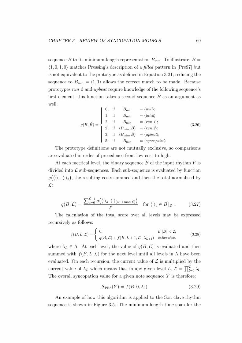
CHAPTER 3. REVIEW OF SYNCOPATION MODELS 60
sequence B to its minimum-length representation Bmin. To illustrate, B =
〈1, 0, 1, 0〉 matches Pressing’s description of a filled pattern in [Pre97] but
is not equivalent to the prototype as defined in Equation 3.21; reducing the
sequence to Bmin = 〈1, 1〉 allows the correct match to be made. Because
prototypes run 2 and upbeat require knowledge of the following sequence’s
first element, this function takes a second sequence B as an argument as
well.
g(B, B) =
0, if Bmin = 〈null〉;1, if Bmin = 〈filled〉;2, if Bmin = 〈run 1〉;2, if 〈Bmin, B〉 = 〈run 2〉;3, if 〈Bmin, B〉 = 〈upbeat〉;5, if Bmin = 〈syncopated〉
(3.26)
The prototype definitions are not mutually exclusive, so comparisons
are evaluated in order of precedence from low cost to high.
At each metrical level, the binary sequence B of the input rhythm Y is
divided into L sub-sequences. Each sub-sequence is evaluated by function
g(〈·〉1, 〈·〉2
), the resulting costs summed and then the total normalised by
L:
q(B,L) =
∑L−1a=0 g
(〈·〉a, 〈·〉(a+1 mod L)
)L
for 〈·〉a ∈ B‖L . (3.27)
The calculation of the total score over all levels may be expressed
recursively as follows:
f(B,L,L) =
{0, if |B| < 2;
q(B,L) + f(B,L+ 1,L · λL+1) otherwise.(3.28)
where λL ∈ Λ. At each level, the value of q(B,L) is evaluated and then
summed with f(B,L,L) for the next level until all levels in Λ have been
evaluated. On each recursion, the current value of L is multiplied by the
current value of λL which means that in any given level L, L =∏L
l=0 λl.
The overall syncopation value for a given note sequence Y is therefore:
SPRS(Y ) = f(B, 0, λ0) (3.29)
An example of how this algorithm is applied to the Son clave rhythm
sequence is shown in Figure 3.5. The minimum-length time-span for the

CHAPTER 3. REVIEW OF SYNCOPATION MODELS 61
Figure 3.5: Example calculation of the Pressing syncopation measure for theSon clave rhythm-pattern. In each metrical level, the matching prototypes foreach subdivision are shown.
sequence has |T | = 16. The results are summed in each level and nor-
malised by L giving SPRS(Y ) = 21
+ 72
+ 124
+ 58
= 9.125. Note that for
this analysis Λ = 〈1, 2, 2, 2〉, we do not need to analyse at levels lower
than eighth-notes because all spans would be nulls at lower levels for this
rhythm-pattern.
3.2.3 Toussaint 2002 ‘Metric Complexity’ (TMC)
Toussaint’s metric complexity measure [Tou02] is another model that uses
metrical hierarchy to calculate a syncopation prediction. In this model,
the metrical weights are defined as wL = Lmax − L + 1 so the highest
weight will be w0 and the lowest will be wLmax = 1.
The model first defines a measure of metricity (metrical simplicity)
ϕ(B,HLmax) for binary sequence B which is the sum of the weights for
each note; simpler rhythm sequences will have notes at stronger time
positions in the hierarchy and hence a higher metricity score
ϕ(B,HLmax) =
|B|−1∑m=0
bmhm (3.30)
where HLmax is the sequence of metrical weights as defined in Equation 3.17
and Lmax is chosen such that |HLmax| = |B|. The hypothesis of the model
is that the level of metrical complexity (i.e. syncopation) is the difference
between the metricity for B and the maximum possible metricity for a

CHAPTER 3. REVIEW OF SYNCOPATION MODELS 62
sequence containing the same number of notes
STMC(Y ) = max(ϕ(B,HLmax)
)− ϕ(B,HLmax) (3.31)
∀B ∈ {B :∑m
bm =∑m
bm} where bm ∈ B, bm ∈ B
For example, the Son clave rhythm from Figure 3.2c has 4/4 time-
signature and |Bmin| = 16 so we require L ∈ [0, 4] to represent its metrical
hierarchy. The parameters for the calculation are therefore
W = 〈5, 4, 3, 2, 1〉, Λ = 〈1, 2, 2, 2, 2〉,
H4 = 〈5, 1, 2, 1, 3, 1, 2, 1, 4, 1, 2, 1, 3, 1, 2, 1〉,
Bmin = 〈1, 0, 0, 1, 0, 0, 1, 0, 0, 0, 1, 0, 1, 0, 0, 0〉.
The metricity will therefore be 5 + 1 + 2 + 2 + 3 = 13 while the maximum
metricity score for a five-note rhythm would be 5+4+3+3+2 = 17. The
syncopation prediction STMC for the Son clave rhythm would therefore be
17− 13 = 4.
3.2.4 Sioros and Guedes 2011 (SG)
The most recent model in our study, Sioros and Guedes [SG11, SHG12]
also uses metrical hierarchy to determine syncopation. This model has
three main hypotheses: First, accenting of notes affects perceived syn-
copation and should be included in the model (the only model in this
study to do so, but it should be noted that the implementation of the
SG model used in the evaluation in Chapter 5 does not include it because
our chosen rhythm stimuli have equal velocity notes throughout). Second,
humans try to minimise the syncopation of a particular note relative to
its neighbours in each level of the metrical hierarchy. Third, syncopations
at the beat level are more salient than those that occur in higher or lower
metrical levels so the outcome should be scaled to reflect this [SMC+13].
The metrical weights for this model are wL = L for all wL ∈ W . To
calculate the syncopation score5, we first define a function ϑ(m, m) that
5The original description of the algorithm in [SG11, SHG12] is mostly given in prose buta Max/MSP patch and C++ source code for a Max/MSP external has been made availableonline at [Sio11] from which our mathematical formulation has been derived.

CHAPTER 3. REVIEW OF SYNCOPATION MODELS 63
calculates a difference level factor between two notes in velocity sequence
V with indices m and m,
ϑ(m, m) = (vm − vm)
(β|hm − hm|
4+ 1− β
)(3.32)
where v ∈ V , h ∈ HLmax and β is a weighting factor.
To obtain the syncopation score for a note at a given metrical level `,
we define a function u(m, `) that calculates the average of the difference
between the note at index m and its neighbours in the same metrical level:
u(m, `) =γ.ϑ(m, %(m, `)
)+ ϑ(m, ρ(m, `)
)γ + 1
(3.33)
where a weighting factor γ is included to reduce the contribution of the
previous note, a function %(m, `) calculates the index of the previous note:
%(m, `) = arg maxm mod |V |
(h(m mod |V |) ≤ ` , m < m) (3.34)
and a second function ρ(m, `) calculates the index of the next note:
ρ(m, `) = arg minm mod |V |
(h(m mod |V |) ≤ ` , m > m). (3.35)
Values for the weighting factors are reported in [SG11] as β = 0.5 and
γ = 0.8.
A note may exist in multiple levels of the hierarchy and thus the syn-
copation score sm is calculated by finding the minimum value of u(m, `)
for each level of the hierarchy for which the note is a member:
sm =
{0, if vm = 0;
min(u(m, `)
)∀{` : ` ∈ [hm, hmax]
}otherwise.
(3.36)
where
hmax = max(hm ∈ HLmax) (3.37)
Figure 3.6 demonstrates calculation of syncopation scores for the Son clave
rhythm from Figure 3.2c. After personal communication with George
Sioros [Sio14] we have used Λ = 〈1, 2, 2, 2, 2〉 as our metrical hierarchy
to implement the SG algorithm. It should be noted, however, that an
alternative hierarchy Λ = 〈2, 2, 2, 2〉 has been used in examples in [SG11]

CHAPTER 3. REVIEW OF SYNCOPATION MODELS 64
Figure 3.6: Sioros and Guedes syncopation scores and potentials for the Sonclave rhythm. The metrical hierarchy is generated and the minimum syncopa-tion score sm for each note is calculated by comparing it against its neighboursin each of the metrical levels in which it resides (see Equation 3.36). Eachscore is then multiplied by the syncopation potential φm and the results aresummed to give the total syncopation value for the rhythm-pattern, in thiscase SSG = 1.698.
and [SHG12] which produces a tree with two top-level nodes. This is
explained in [SMC+13] as an attempt to correct for the effect of tempo on
syncopation; an effect that has yet to be studied formally.
Once the syncopation scores have been calculated for each note in the
sequence, they are weighted by a syncopation potential φm according to
their metrical level:
φm = (1− 0.5hm) (3.38)
The total syncopation prediction from this model for a given sequence is
the sum of all weighted scores for individual notes:
SSG(Y ) =
|V |−1∑m=0
smφm (3.39)
Separate normalisation approaches for this model are reported in [SG11]
and [SHG12] but, on the advice of [Sio14], we use the absolute value for
our evaluation in Chapter 5.

CHAPTER 3. REVIEW OF SYNCOPATION MODELS 65
3.2.5 Keith 1991 (KTH)
The hypothesis of Keith’s model [Kei91] is that syncopations occur where
notes start or end at off-beat positions. Two individual types of syncopated
event are defined and given a weight k. These two types are hesitation,
where a note ends off the beat (k = 1) and anticipation, where a note
begins off the beat (k = 2). Where a note exhibits both a hesitation and
an anticipation, a syncopation is said to occur and the weights are summed
to give k = 3. (See Figure 2.12 for examples.) Keith constrains the model
to time-signatures where the number of beats per bar is a power of two.
The first step in calculating this model is to find ∆t for time-span T
such that:
|T | = arg min2ξ
(2ξ ≥ |Tmin|) (3.40)
We may then calculate a value cn for each note yn which is the highest
power of two less than or equal to its duration:
cn = arg max2ξ
(2ξ ≤ ytdn∆t
) (3.41)
In this model, the onset ytsn or end time (ytsn + ytdn ) are considered off
beat if they are not a multiple of cn∆t. Note that Keith’s model assumes
note duration to be the inter-onset interval between consecutive notes i.e.
ytdn = ytsn+1 − ytsn . Using this rule, we may define ‘off-beat’ functions on
and en that determine whether the onset or end of note yn are off the beat
respectively:
on =
{0, if ytsn
∆tmod cn = 0;
2, otherwise (anticipation)(3.42)
and
en =
{0, if (ytsn +y
tdn )
∆tmod cn = 0;
1, otherwise (hesitation)(3.43)
The Keith syncopation weight for note yn is therefore
kn = on + en. (3.44)
For a sequence Y comprising |Y | notes, the Keith syncopation score SKTH(Y )
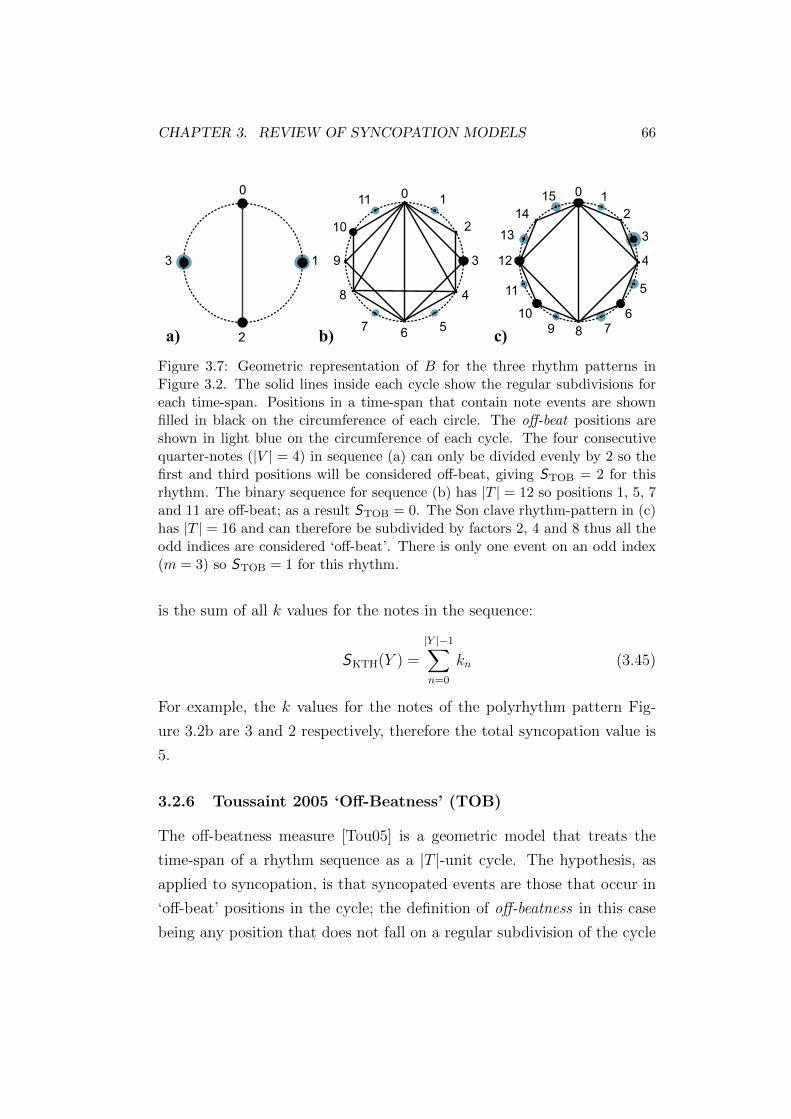
CHAPTER 3. REVIEW OF SYNCOPATION MODELS 66
0
8
412
12
3
5
67
10
11
13
14150
6
39
1
2
4
57
8
10
110
2
13
a) b) c) 9
Figure 3.7: Geometric representation of B for the three rhythm patterns inFigure 3.2. The solid lines inside each cycle show the regular subdivisions foreach time-span. Positions in a time-span that contain note events are shownfilled in black on the circumference of each circle. The off-beat positions areshown in light blue on the circumference of each cycle. The four consecutivequarter-notes (|V | = 4) in sequence (a) can only be divided evenly by 2 so thefirst and third positions will be considered off-beat, giving STOB = 2 for thisrhythm. The binary sequence for sequence (b) has |T | = 12 so positions 1, 5, 7and 11 are off-beat; as a result STOB = 0. The Son clave rhythm-pattern in (c)has |T | = 16 and can therefore be subdivided by factors 2, 4 and 8 thus all theodd indices are considered ‘off-beat’. There is only one event on an odd index(m = 3) so STOB = 1 for this rhythm.
is the sum of all k values for the notes in the sequence:
SKTH(Y ) =
|Y |−1∑n=0
kn (3.45)
For example, the k values for the notes of the polyrhythm pattern Fig-
ure 3.2b are 3 and 2 respectively, therefore the total syncopation value is
5.
3.2.6 Toussaint 2005 ‘Off-Beatness’ (TOB)
The off-beatness measure [Tou05] is a geometric model that treats the
time-span of a rhythm sequence as a |T |-unit cycle. The hypothesis, as
applied to syncopation, is that syncopated events are those that occur in
‘off-beat’ positions in the cycle; the definition of off-beatness in this case
being any position that does not fall on a regular subdivision of the cycle

CHAPTER 3. REVIEW OF SYNCOPATION MODELS 67
length |T |. The off-beatness ςm of a position can be calculated as follows:
ςm =
0, if m mod z = 0
∀ {z : |T | mod z = 0 : 1 < z < |T |}1, otherwise
(3.46)
For example, a time-span sequence of |T | = 12 can be evenly subdivided
by the values two, three, four and six. Therefore the dimensions of the
sequence for which ςm 6= 0 are those that are not divisible by these factors
(i.e. dimensions 1, 5, 7 and 11) and so these are considered to be off-beat
positions. Using this model, the total syncopation score for a sequence
Y may be calculated by summing the number of syncopated events it
contains:
STOB(Y ) =
|B|−1∑m=0
bmςm (3.47)
Figure 3.7 shows a visual representation of the off-beatness measure ap-
plied to the three rhythm-pattern examples introduced in Figure 3.2.
3.2.7 Gomez 2005 ‘Weighted Note-to-Beat Distance’ (WNBD)
The WNBD model of Gomez et al. [GMRT05] defines note events that
start in between beats in the notated meter to be ‘off-beat’ thus leading
to syncopation. The syncopation value for a note is determined by its
distance from the nearest beat6, notes being assumed to be contiguous in
time with one ending as the next begins.
The position of a note yn may be defined in terms of a distance measure
d relative to its nearest beats µi and µi+1 (i.e. the onset of yn falls between
µi and µi+1, see Figure 3.8).
µi ≤ ytsn ≤ µi+1 (3.48)
d(yn, µi) =ytsn − µiµi+1 − µi
(3.49)
6Gomez et al. use the term ‘strong-beat’ in their paper but clarify that they mean the met-ric pulse, rather than strong-beats as defined with respect to metrical hierarchy as discussedin Section 3.1.4

CHAPTER 3. REVIEW OF SYNCOPATION MODELS 68
A
μ i
yn
d( ) A
μ i+2μ i+1
ts
yntd
,μiyn d( ) ,μi+1yn
Figure 3.8: Illustration of the relationship between note yn and the beats fromµi to µi + 2.
To calculate the WNBD measureW(yn) for note yn, we first find T (yn),
the distance from yn to its closest beat.
T (yn) = min(d(yn, µi), d(yn, µi+1)) (3.50)
The value of W(yn) can then be found by
W(yn) =
0, if d(yn, µi) = 02
T (yn), if µi+1 < ytsn + ytdn ≤ µi+2
1T (yn)
, otherwise
(3.51)
For a note that starts on the beat (i.e. d(yn, µi) = 0), W(y) will be
0. For a note that starts off the beat ( i.e. d(yn, µi) 6= 0) and ends on
or before the next beat µi+1, W(yn) will be 1T (yn)
. Where a note is held
on past µi+1 but ends on or before µi+2, W(yn) is 2T (yn)
, weighting tied
notes more highly than others. For notes that end after µi+2, W(yn) is
set to 1T (yn)
. If Y is a sequence of |Y | notes, the WNBD score for Y is the
normalised sum of the W values for each note in the sequence:
SWNBD(Y ) =1
|Y |
|Y |−1∑n=0
W(yn) (3.52)
To illustrate, the W values for the notes of the Son clave example in
Figure 3.2c are 0, 8, 4, 2 and 0 respectively, so the WNBD predicted
syncopation is 0+8+4+2+05
= 2.8.
3.3 Summary
This chapter developed a consolidated mathematical representation for
rhythm, metrical hierarchy and seven syncopation models. The main

CHAPTER 3. REVIEW OF SYNCOPATION MODELS 69
purpose of this is to provide an in-depth review and to clarify ambigu-
ities of the syncopation models that are frequently used in other stud-
ies. The secondary purpose is to implement these syncopation models
into programming codes by transferring the corresponding mathematical
equations. The implementation of the models facilitates the evaluation of
these models in the later chapters. In the next chapter, we will switch to
the investigation of syncopation in the area of perception, which enables
a direct and formal evaluation of the syncopation models reviewed in this
chapter.
Chapter 4
Syncopation and the score
In this chapter, we begin to explore syncopation perception: we manipu-
late the rhythmic score as an objective correlate of perceived syncopation.
The main method in our experiment was to ask listeners to rate the de-
gree of syncopation they perceived in response to a rendering of each score.
Section 4.1 specifies the materials and the procedure in the experiment.
We test the hypothesis that the following will have a degree of influence
on perceived syncopation: i) time-signature, ii) whether the down-beat is
present or missing, iii) presence of polyrhythms or monorhythms (which
we will define here as any rhythm-pattern which is not polyrhythmic)
and finally iv) within-bar location of rhythm-components. Results are
discussed in Sections 4.2 and 4.3.
4.1 Experiment 1: Score
We asked musicians to give informed ratings of perceived syncopation for
renderings of various three-bar scores. The ratings were taken over a
fixed, five-point rating scale. In this experiment we required the listen-
ers to judge a large number of rhythms, with a potentially large range
of syncopation ratings. The fixed rating scale was intended to provide
the minimum complexity in the experimental interface and the maximum
efficiency during the procedure; the aim being that listeners would not
be hampered by unnecessary precision in the interface and would be able
to focus on their immediate perceptual response. We acknowledge that
such methods may be prone to minor biases (e.g. range bias, end-point
bias [Pou89]) but we argue that such biases are offset by the overall scale
70

CHAPTER 4. SYNCOPATION AND THE SCORE 71
of the syncopation continuum and stimuli. In other words, the stimuli
we employed ranged between not syncopated and highly syncopated, so we
trade finer detail in the data for an efficient method. All listeners used
the whole range of the scale (i.e. each listener gave at least one minimum
and one maximum rating).
4.1.1 Participants
We recruited ten participants, nine male and one female, with an average
age of 30 years (standard deviation 5.8 years). All participation was vol-
untary (unpaid). In order to maximize the degree of homogeneousity of
the group, all participants are trained musicians.Their musical training in-
cluded formal performance and theory over a range of instruments, music
production and engineering. All participants had trained for an average
of 15 years (standard deviation 5 years). Six of them reported proficiency
in multiple instruments. All participants confirmed that they were con-
fident in their understanding and rating of syncopation. All participants
reported normal hearing.
4.1.2 Stimuli
Each score, rendered to produce a single stimulus, was constructed of
three bars. The first bar was always metronome alone (either 4/4 or
6/8). The second and third bars were repetitions of a one-bar rhythm-
pattern constructed from concatenation of two basic, half-bar rhythm-
components. Figure 4.1 provides a schematic diagram which illustrates the
steps taken when generating the stimuli. First, various half-bar rhythm-
components (Figure 4.1a) were paired to produce one-bar rhythm-patterns
(Figure 4.1b). The rhythm-components were categorised as either binary
(two notes) or ternary (three notes). Next, the rhythm-patterns were
concatenated and a metronome was added to produce the final score (Fig-
ure 4.1c). Finally, the stimulus was rendered to produce the acoustic wave-
form (Figure 4.1d) which was ultimately heard by the listener. Rhythms
were played concurrently with the metronome (following the single bar of
introductory metronome) (Figure 4.1c).

CHAPTER 4. SYNCOPATION AND THE SCORE 72
)) ))A)))A E I
) A ) AA) A)B F J
A ) A )AA ))C G K
A A A AAA A)D H L
Binary Ternary
Rhythm-components
Complete scores
Rhythm-patterns
A A A )DCBinary + Binary
A ) A ) AyCJBinary + Ternary
A )AA A)HKTernary + Ternary
AIIII W W W W W W W W W'W W W
A
metronome
rhythm
DC DC
A ) A )A AA=140bpm = 429.6ms
X'
KM X X X X X X X X X X X X X X X X X$ $ *$ $* $ $ *$ $*KM
HK HK=280bpm = 214.3ms $
Missing down-beat
AII )II W W W W W W W W W
' A ) A
W W Wy A ) A ) A
yCJ CJA=140bpm = 429.6ms
Polyrhythm
Rendered stimulus
Example CJ: duration = 5.1 seconds
(a)
(b)
(c)
(d)
Figure 4.1: Construction of stimuli. A schematic diagram illustrating the pro-cess of generating the stimuli. (a) Rhythm-components. Ten basic rhythm-components are created, categorised into binary or ternary depending on thenumber of events. (b) Rhythm-patterns. Half-bar rhythm-components arepaired to create one-bar rhythm-patterns. (c) Complete scores. Rhythm-patterns (and metronome) are used to produce a three-bar score, includingrhythm-patterns featuring missing down-beats and polyrhythms. The combi-nations of two binary or one binary and one ternary rhythm-components arenotated with a time-signature of 4/4; two ternary rhythm-components fit into6/8. The tempo for both signatures is 140 quarter-note per minute (QPM). (d)Rendered stimulus. The score is rendered as a waveform.

CHAPTER 4. SYNCOPATION AND THE SCORE 73
Figure 4.1a shows the ten half-bar rhythm-component notations (A-
L) from which concatenated whole-bar pairs were produced in all possible
combinations. These base rhythm-components include notations featuring
rhythmic structures that are anticipated to result in syncopation: missing
down-beats, off-beat notes and polyrhythms when presented in relation to
a metronome. Example rhythm-pattern pairings are given in Figure 4.1b.
Rhythm-patterns composed of a given pair of rhythm-components were
presented separately in both forward and reverse order (e.g. CJ and JC).
By comparing such pairs, we are able to investigate the effect of location
(e.g. of missing strong-beats) within the bar.
Scores for example stimuli, including metronome, are given in Fig-
ure 4.1c. There were 99 unique pairs, after excluding redundant patterns
E and I, which were replaced with A and C respectively (which are equiv-
alent in 4/4). The time-signature was set to 6/8 for all combinations of
two ternary rhythm-components and 4/4 for the rest. As a result, the
overall stimuli comprises three rhythm-categories: 4/4 monorhythms, 6/8
monorhythms and (3:2) 4/4 polyrhythms. The potential combinations
that result in (2:3) 6/8 polyrhythms are excluded in order to limit the
length of the required listening test. While this combination of stimuli
provides a representative range of rhythm-patterns in two time-signatures,
it should be noted the proportions of examples between 4/4 and 6/8 time-
signatures, and between monorhythms and polyrhythms differ.
The stimuli were rendered (synthesised) at a sampling rate of 44.1 kHz
16-bit using MIDI sequencing (see Figure 4.1d for an example waveform).
A percussive snare drum sample was used for the musical rhythm and a
‘cow-bell’ sample was used for the metronome. We chose a uni-tone per-
cussive drum sound for rhythm-patterns in order to avoid the interaction
between pitch and rhythm, and to remove confounding factors such as
note duration [Lon04, p.28].
The snare drum sample was approximately 700 milliseconds (ms) in
duration, with approximately 7 ms attack, 130 ms sustain and 450 ms
decay. The metronome sample was relatively impulsive and of approxi-
mately 20 ms duration. The metronome was dynamically accented on the

CHAPTER 4. SYNCOPATION AND THE SCORE 74
first beat of the bar and was also accented in pitch; the fundamental fre-
quency of the accented note was 940 Hz and the remaining notes were of
680 Hz. Thus, our metrical cue (metronome) was clearly differentiable (by
timbre and pitch) from the overlaid drum rhythm. By accenting the first
beat of metronome in 6/8, we do not explicitly rule out a 3/4 grouping of
beats.
The tempo of the metronome was set to 140 BPM for all rhythm-
patterns in a time-signature of 4/4 and 280 BPM for those in 6/8. This
corresponds to an interval of 428.6 ms per quarter-note in both time sig-
natures. In 4/4 the metronome beat quarter-notes at this interval and in
6/8 it beat eighth-notes (i.e. an interval of 214.3 ms per beat). Hence, in
4/4 stimuli that contained polyrhythmic components, the interval between
triplet quarter-notes was 285.7 ms. The resulting stimuli durations (per
trial) were 5.1 seconds in 4/4 (i.e. three bars of four quarter-note beats)
and 3.9 seconds in 6/8 (i.e. three bars of six eighth-note beats).
4.1.3 Procedure
Stimuli were presented individually and at the instigation of the listener.
All stimuli were presented within a single block. For each trial, the listener
gave a rating between zero and four, where zero indicated no syncopation
and four indicated maximum syncopation. The listener was free to lis-
ten to each pattern repeatedly before giving their rating. The stimuli
were presented in randomised order (i.e. a different order for each lis-
tener). Before the experimental session, the listeners heard a broad range
of example stimuli and were given a practice run (the resulting data was
discarded). Each participant was free to adjust the sound level at any time
so as to be comfortable. Headphones were used to present the stimuli. All
presentation was dichotic (the same in both ears). Tests were completed
in approximately 30-50 minutes. Listeners were encouraged to take breaks
during the session.

CHAPTER 4. SYNCOPATION AND THE SCORE 75
(a)
(b)
Figure 4.2: Group mean syncopation ratings for rhythm-patterns. (a) A matrixshowing group mean syncopation ratings for rhythm-patterns. The upper tri-angle of the matrix refers to rhythm-patterns where the horizontal axis denotesthe first rhythm-component of the rhythm-pattern, and where the vertical axisdenotes the second rhythm-component. For the lower triangle of the matrix thereverse is true. This provides a general way to compare the mean ratings be-tween the two orders of presentation for any given pair of rhythm-components.Same rhythm-component pairs (e.g. BB) are shown in grey. Note that thepair AA is excluded because it represents a full bar of rests. (b) A map ofthe matrix shown in (a), broken down into regions corresponding to score fea-tures: polyrhythmic and monorhythmic patterns in both 4/4 and 6/8. Thismap illustrates how the data is categorised in the subsequent analyses.

CHAPTER 4. SYNCOPATION AND THE SCORE 76
Figure 4.3: Categorical analysis. Group mean and 95% confidence intervals forpooled ratings, averaged for each listener, composed (selectively) for compari-son of ratings for all stimuli categorised within the following paired conditions:monorhythms in 4/4 versus those in 6/8 (see Figure 4.2b), polyrhythms ver-sus monorhythms, down-beat missing versus down-beat present, strong-beatmissing versus strong-beat present. * denotes significance (p < 0.05, WilcoxonSigned-Rank Test, uncorrected).
4.2 Results
Figure 4.2a broadly summarises the syncopation ratings in a matrix rep-
resentation of the group mean ratings for each rhythm-pattern. The hor-
izontal axis shows the first rhythm-component of the respective rhythm-
pattern, and the vertical axis shows the second rhythm-component. There-
fore, the upper-left triangular area of the matrix corresponds to the op-
posite pair-wise ordering of rhythm-components within the same rhythm-
pattern to those in the lower-right triangular area of the matrix. Fig-
ure 4.2b provides a ‘map’ corresponding to Figure 4.2a, which illustrates
grouping of the ratings for subsequent analyses. The average correlation
coeffecient (Spearman) between each pair of listeners in the group is 0.47,
suggesting that the ratings are reasonablly consistent between listeners.
Figures 4.3 and 4.4 show various selective groupings of the ratings data
(across all listeners), where the data (N =10 listeners) were selected to
test the following hypotheses: 1) 6/8 is more syncopated than 4/4; 2)
polyrhythms are more syncopated; 3) missing down-beats result in synco-
pation; and 4) switching component order affects syncopation.

CHAPTER 4. SYNCOPATION AND THE SCORE 77
Figure 4.4: Syncopation by rhythm-component. Mean and 95% confidenceintervals for ratings pooled by rhythm-component. For each distribution, allratings for rhythm-patterns featuring each respective rhythm-component wereselected and separated into groups by location of the rhythm-component withinthe rhythm-pattern (e.g. AB + AC + AD versus BA + CA + DA.). Greyindicates the location of the rhythm-component is on the first half of the bar,and pink indicates that on the second half. * denotes significance (p < 0.05,Wilcoxon Signed-Rank Test, uncorrected).
4.2.1 6/8 is more syncopated than 4/4
For each listener, all ratings were separately pooled and averaged for all
stimuli featuring time-signatures of 4/4 and 6/8. This gives a pair of

CHAPTER 4. SYNCOPATION AND THE SCORE 78
ratings distributions which may be compared to see whether either time-
signature was more or less highly rated (for syncopation). Figure 4.3 shows
that 6/8 is more highly rated than 4/4 (W = 1, Z = −2.55, p < 0.01, r =
0.81, Wilcoxon Signed-Rank Test).
4.2.2 Polyrhythms are more syncopated
Next, for each listener, all ratings were separately pooled and averaged for
all stimuli that constituted a polyrhythm (i.e. in 4/4 see Figure 4.2b and
all stimuli that did not. The resulting ratings distributions are likewise
compared to establish the existence of significant differences that may
indicate a pre-disposition of polyrhythms to result in the perception of
syncopation. Figure 4.3 shows that polyrhythms are much more highly
rated than monorhythms (W = 55, Z = 2.8, p < 0.01, r = 0.89, Wilcoxon
Signed-Rank Test).
4.2.3 Missing down-beats result in syncopation
For each listener, ratings for all rhythm-patterns featuring ‘missing down-
beats’ were pooled and averaged. The same pooled averages were cal-
culated for rhythm-patterns not containing missing down-beats. The re-
sulting group ratings distributions are compared in Figure 4.3 and show
that rhythm-patterns featuring missing down-beats are more highly synco-
pated than those not featuring missing down-beats (W = 54, Z = 2.7, p <
0.01, r = 0.85, Wilcoxon Signed-Rank Test). A similar analysis was per-
formed for all pairs featuring missing strong-beats, with a similar (albeit
not significant) outcome (p > 0.05, Wilcoxon Signed-Rank Test).
4.2.4 Switching component order affects syncopation
In order to investigate the effect of location of each rhythm-component
within the rhythm-pattern, the ratings resulting from each of the two
possible orders were compared. Where certain rhythm-components are
associated with high degrees of syncopation (e.g. rhythm-components
which feature a missing down-beat), we can observe the effect of loca-
tion within the rhythm-pattern (bar). For each listener, ratings for all

CHAPTER 4. SYNCOPATION AND THE SCORE 79
rhythm-patterns featuring a given rhythm-component were pooled and
averaged for both possible locations of a given rhythm-component (within
the rhythm-pattern). The group mean and 95% confidence intervals for
the resulting distributions are plotted in Figure 4.4. Only rhythm-patterns
featuring rhythm-components A (W = 34.5, Z = 2.31, p < 0.05, r = 0.73),
G (W = 44, Z = 2.57, p < 0.05, r = 0.81), H (W = 41, Z = 2.15, p <
0.05, r = 0.68) and J (W = 0, Z = −2.67, p < 0.05, r = 0.85) showed sig-
nificant differences (Wilcoxon Signed-Rank Test, uncorrected) which held
regardless of the other rhythm-components within the various rhythm-
patterns. The average ratings were larger when A, G and H were in the
first half of the bar, but the opposite was true for J. The overall shape of
the graph is consistent with the comparison of missing down-beats shown
in Figure 4.3, in that rhythm-patterns featuring rhythm-components A,
B, F, G and H show higher mean syncopation ratings.
In order to find out exactly which rhythm-patterns were sensitive to
location of the rhythm-components, the analysis was refined to focus on
the pair-wise comparison of ratings for each rhythm-pattern between the
two possible orders of the rhythm-components. Figure 4.5 shows a matrix
plot of the difference in group mean rating for each rhythm-pattern, caused
by change in the rhythm-component order (i.e. within the bar). Signif-
icant changes in rating are indicated with overlaid triangles (p < 0.05,
Wilcoxon Signed-Rank Test, uncorrected). Rhythm-components which
significantly changed when the rhythm-component order was switched
were: AC (W = 28, Z = 2.56, p < 0.05, r = 0.81), AD (W = 15, Z =
2.21, p < 0.05, r = 0.7), BH (W = 0, Z = −2.21, p < 0.05, r = 0.69), FG
(W = 0, Z = −2.22, p < 0.05, r = 0.7), GJ (W = 34, Z = 2.28, p <
0.05, r = 0.72) (see Figure4.5b). Again, significant changes occur for
rhythm-patterns featuring rhythm-components A, B, F, G, H, all of which
feature missing down-beats. In other words, rhythm-components resulting
in missing down-beats contribute significantly more to the perception of
syncopation than the same rhythm-components in the second half of the
bar (rhythm-pattern).

CHAPTER 4. SYNCOPATION AND THE SCORE 80
(a)
(b)
Figure 4.5: Pair-wise changes in ratings when rhythm-component order wasswitched. (a) The change in group mean rating (for each rhythm-pattern)caused by switching the rhythm-component order (i.e. this is equivalent to asubtraction of the lower-triangle ratings of Figure 4.2a from the upper-triangleratings of Figure 4.2a). Triangles denote significance (p < 0.05, WilcoxonSigned-Rank Test, uncorrected). Interestingly, the significant changes (whenorder was switched) correspond to missing down-beat rhythm-patterns. (b)The notations for each pair of rhythm-patterns that reached significance.
4.3 Discussion
In this chapter, we have shown that there is more potential for syncopation
in 6/8 in polyrhythms and in rhythms featuring a missing down-beat. We
have also shown that the location of rhythm-components that give rise to

CHAPTER 4. SYNCOPATION AND THE SCORE 81
syncopation is critical to its perceived degree. These results demonstrate
that syncopation cannot simply be predicted (i.e. in a model) by summa-
tion of ‘syncopation values’ calculated for individual notes according to
the relationship between each note and the assumed metrical structure.
We also identify three questions for further investigation: i) Is syncopa-
tion tempo-dependent? ii) Why do the 4/4 monorhythm patterns exhibit
lower syncopation levels than monorhythms in 6/8? iii) Do listeners re-
interpret the meter of a given rhythm-pattern in order to reduce the level
of perceived syncopation?
4.3.1 4/4 versus 6/8
We employ the standard terminology for meters (i.e. time-signatures)
in Western music [Lon04]; the terms duple and triple to refer to two-
and three-beat bars respectively, and the terms simple and compound to
refer to the binary and ternary subdivision of beats in a bar. Here, we
investigated the signatures 4/4, which is simple-duple meter (i.e. two
groups of two quarter-notes), and 6/8 which is compound-duple meter
(two groups of three eighth-notes).
6/8 monorhythmic patterns were rated as more syncopated than those
in 4/4 (Figure 4.3). There are several potential explanations for this obser-
vation. First, given that a time-signature must be rendered (or performed)
according to a specified tempo, a major difference between the stimuli in
these two time-signatures is their speed. The beat rate in the 6/8 stimuli
was twice as fast as those in 4/4 because eighth-notes are half as long as
quarter-notes and the tempi were chosen to maintain the same duration
for quarter-notes in both.
It has been shown that tempo influences various aspects of music per-
ception, such as rhythm recognition [Han93], pitch perception [DGM88],
music preference [LeB81] and perception of emotion in music [vZWvdB11].
In particular, the ability to discriminate differences between rhythms [Han93],
perception of meter from polyrhythms [HO81, HL83] and production of
rhythmic timing [RWD02, DH94] all appear to be influenced by tempo.
Therefore, we expect that tempo may affect the perceived syncopation

CHAPTER 4. SYNCOPATION AND THE SCORE 82
and this may explain the higher ratings in 6/8 than in 4/4.
Another possible reason for higher ratings in 6/8 than 4/4 may be
that the rhythmic structure of 4/4 is inherently less ambiguous – 4/4 is
simple-duple meter (duple subdivision of duple) and 6/8 is compound-
duple meter (triple subdivision of duple). Several studies have shown that
listeners of all ages naturally show bias towards processing (and preference
for) rhythms that incorporate binary rather than ternary metrical subdi-
visions [LJ83, PE85, Dra93, BT06]. Indeed, it has been shown that the
accuracy of rhythm reproduction in binary subdivisions of beat is higher
than ternary subdivisions [Dra93]; people are inclined to tap on the bi-
nary subdivisions to isochronous auditory sequences when they are asked
to tap at a fast rate [Dra97]; also, both adults and infants react more
quickly and accurately to the alterations in pitch, melody and harmony
in binary meter than in triple meter [BT06, SC89].
Syncopation has been associated with human metrical processing [FR07,
SP00, SK01, TS03], and metrical processing has also been related to
time-signature [LJ83, PE85, Dra93, BT06, SC89]. Our finding, that 6/8
monorhythms are perceived as more syncopated than those in 4/4, sug-
gests that time-signature and perceived syncopation are inherently related
and hence may explain the previously reported relationship between met-
rical processing and time-signature.
4.3.2 Missing down-beats
Syncopation models predict that missing strong-beats (the absence of
events at strong metrical positions) result in syncopation [LHL84]. The
models also predict that a missing down-beat (the first beat of the bar)
generates a higher degree of syncopation than a missing strong-beat in
a lower metrical level (e.g. the third quarter-note in 4/4 or the fourth
eighth-note in 6/8) result in syncopation.
In general, our results agree with the modelling predictions; the pat-
terns with missing down-beats tend to have higher average ratings (Fig-
ure 4.3). This is also clear in Figure 4.4, which shows that rhythms starting
with a rest (components A, B, F, G and H) contribute to higher average

CHAPTER 4. SYNCOPATION AND THE SCORE 83
ratings, while patterns including components C, D, K or L have relatively
low average ratings (these do not start with a rest). However, we did not
find strong evidence suggesting that rhythms that feature missing strong-
beats have an effect on syncopation. This may be due to the small number
of participants in the study.
The latter modelling prediction, that missing down-beats will have a
higher degree of syncopation than equivalent missing strong-beats, is par-
tially supported in Figure 4.4: Rhythm-patterns beginning with rhythm-
components A, G and H (which contain missing down-beats) have higher
average ratings than those with A, G or H respectively in the second half
(Figure 4.4). The pair-wise comparisons (in Figure 4.5) for pairs AC/CA,
AD/DA and GJ/JG also support this.
4.3.3 Possible interpretation of 6/8 as 3/4
In Figure 4.5, we can observe a significant difference in syncopation rat-
ings for the 6/8 patterns FG/GF and GJ/JG depending on component
order. We might expect to see this for GJ/JG because GJ has a missing
down-beat whereas JG does not. Note, however, that this does not explain
why other similar 6/8 patterns do not show an equivalent significant dif-
ference. In contrast, FG and GF both exhibit a missing down-beat so it is
interesting that there should be a significant difference (due to switching
order) in this case and prompts further explanation. In listening tests,
Povel and Essens [PE85] found that, given a choice, listeners select the
meter which minimises metrical contradiction (i.e. syncopation). Looking
at the rhythm-patterns in question (notated in Figure 4.5), we can see
that for FG and JG, all the notes fall on strong-beats in 3/4 (i.e. eighth-
note positions 1, 3 and 5 in 6/8) whereas in GF and GJ, this is not the
case. Indeed, using the clock model of Povel and Essens [PE85], patterns
FG and JG are strongly predicted to be interpreted as 3/4 time whereas
GF and GJ would be predicted as 6/8. It is possible therefore that the
listeners are interpreting some 6/8 patterns as 3/4, which would thus re-
duce the anticipated level of syncopation. The clock model also makes
similar predictions with regards to the results shown in Figure 4.4d. The

CHAPTER 4. SYNCOPATION AND THE SCORE 84
ternary components G, H and J show significant differences according to
their location in the bar where other ternary components do not. The
component order corresponding to low syncopation ratings in these cases
may be explained as being a result of listeners interpreting the meter as
3/4. Such metrical interpretation is broadly consistent with the findings
of Hannon et al. [HSEK04], who showed that when judging meter, listen-
ers were more likely to choose 6/8 when the tempo the was fast but more
likely to choose 3/4 when the tempo was slow.
4.3.4 Polyrhythms
Polyrhythms were rated as more syncopated than monorhythms (Fig-
ure 4.3). In music psychology, polyrhythms are usually dealt with as
a separate concept to syncopation [Lon04, LHL84]. However, if we accept
the definition of syncopation as being a contradiction to the prevailing me-
ter, then the introduction of a competing meter (i.e. within a polyrhythm)
would clearly also give rise to this phenomenon. The fact that we found
polyrhythms to be more syncopated than monorhythms suggests that the
challenge to the prevailing meter, from a counter meter, is more sub-
stantial than that caused by emphasising weak-beats over strong-beats in
monorhythms.
In Figure 4.5, one pattern containing a polyrhythm, BH/HB, shows
significant difference when the order of rhythm-components is switched.
Both components of BH/HB are missing the strong-beat yet HB was rated
as significantly more syncopated than BH. This may be explained by the
fact that component B is a monorhythm in 4/4 but H is a polyrhythm
in that meter. When H is placed in the first half of the pattern it is a
polyrhythm that has a missing down-beat, which implies that the synco-
pation is compounded in this case.
4.4 Summary
In this chapter, we evaluated the relationship between notated rhythm
and perceived syncopation. We used a metronome to provide explicit cues

CHAPTER 4. SYNCOPATION AND THE SCORE 85
to the prevailing rhythmic structure (as defined in the time-signature).
Three-bar scores with time-signatures of 4/4 and 6/8 were constructed
using repeated one-bar rhythm-patterns, with each pattern built from ba-
sic half-bar rhythm-components. Our manipulations gave rise to vari-
ous rhythmic structures, including polyrhythms and rhythms with miss-
ing strong- and/or down-beats. Listeners were asked to rate the degree
of syncopation they perceived in response to a rendering of each score.
We observed higher degrees of syncopation in time-signatures of 6/8 for
polyrhythms and for rhythms featuring a missing down-beat. We also
found that the location of a rhythm-component within the bar has a sig-
nificant effect on perceived syncopation.
This experiment also forms a dataset that consists of 99 rhythm-
patterns and the corresponding humans perceptual ratings on syncopa-
tion. In the following chapter, we will give in-depth reviews of several
well-known syncopation models and evaluate them against this dataset.

Chapter 5
Evaluation of the models
The studies in which the syncopation models have previously been evalu-
ated [GTT07, Thu08, SH07] have been tested against measures presumed
to be indirectly related to syncopation; these include rhythmic complexity
and difficulty in rhythm reproduction or rhythm recognition [PE85, Ess95,
SP00, FR07]. In this chapter, we introduce a complete dataset for synco-
pation perception and test the models directly on it. The dataset, detailed
in Section 5.1, is an extension of the work from Chapter 4 where the per-
ception of syncopation was investigated explicitly by asking musicians to
rate the degree of perceived syncopation in response to rhythm-patterns
in time-signatures of 4/4 and 6/8.
Our evaluations in Section 5.2 follow Chapter 4 by splitting the data
into three rhythm-pattern categories: 4/4 monorhythm, 6/8 monorhythm
and 4/4 polyrhythms. Some models are not designed to handle all three
categories, so we present individual results for each model as appropriate.
Finally, we analyse the respective strengths and weaknesses of each model.
5.1 Dataset 1
In Chapter 4, we introduced Experiment 1, in which we asked ten experi-
enced musicians to give informed ratings over a five-point rating scale, of
perceived syncopation for renderings of 99 three-bar scores. We then ex-
tended this experiment to include 12 more rhythm-patterns at the eighth-
note level for a total of 111 rhythms by replicating the methodology in
Section 4.1.
86

CHAPTER 5. EVALUATION OF THE MODELS 87
We recruited a further ten trained musicians, eight male and two fe-
male, with an average age of 32 years (standard deviation 5.2 years). All
participants had trained for an average of 18.5 years (standard deviation
7.9). All of them reported proficiency in multiple instruments. All par-
ticipants confirmed that they were confident in their understanding and
rating of syncopation. Four of them had participated in the previous ex-
periment. All participants reported normal hearing.
As in the part of Experiment 1 that we explored in Chapter 4, each
score, rendered to produce a single stimulus, was constructed of three bars.
The first bar was always metronome alone. The second and third bars
were repetitions of a one-bar rhythm-pattern constructed from concatena-
tion of two basic, half-bar rhythm-components out of ten (see Figure 4.1
for an illustration of the steps taken when generating the stimuli). The
combination of a binary and a ternary rhythm-component in 4/4 meter
creates a polyrhythm. In contrast, a monorhythm is any rhythm-pattern
which is not polyrhythmic, which means that it is constructed from ei-
ther two binary rhythm-components in 4/4 meter or two ternary in 6/8.
The extended 12 rhythm-patterns (4/4 monorhythms) were constructed
from binary rhythm-components A-D (after removing the duplications of
rhythm-patterns formed in the experiment described in Chapter 4), and
each of which was scaled down to a quarter-note-duration in a time sig-
nature of 4/4 to generate eighth-notes (example in Figure 5.1).
The stimuli were rendered (synthesised) at a sampling rate of 44.1 kHz
16-bit using MIDI sequencing. As described in Chapter 4, a percussive
snare drum sample was used for the musical rhythm and a ‘cow-bell’ sam-
ple was used for the metronome. The tempo of the metronome was set to
140 BPM.
The procedure exactly followed that set out in Section 4.1.3; Partic-
ipants were unpaid volunteers and gave informed verbal consent before
the experiment. Participants were free to withdraw at any point. Tests
were arranged informally and conducted at the convenience of the partic-
ipants. Written consent was not deemed necessary due to the low (safe)
sound pressure levels employed in the test. The experimental protocol
(including consent) was approved by the ethics committee of Queen Mary

CHAPTER 5. EVALUATION OF THE MODELS 88
>
* $II 'W W W WII >W W W W >W W W W
$*A=140bpm = 428.6ms * $ $ * * $ $ * * $ $ *BC BC BC BC
Figure 5.1: The example score of rhythm-pattern BCBC. Rhythm-componentsB and C are paired to create a half-bar rhythm-pattern BC; BC is then re-peated once to produce a one-bar rhythm-pattern BCBC. The three-bar scoreis generated from one bar of metronome alone, and two bars of repetitions ofthe one-bar rhythm-pattern BCBC.
A B C D
A
B
C
D
First (and third)
rhythm-component
Se
co
nd
(a
nd
fo
rth
)
rhyth
m-c
om
po
ne
nt
3
2
1
0
Ra
tin
g
Figure 5.2: Group mean syncopation ratings for the extended stimuli. Thismatrix shows the group mean syncopation ratings for the 12 extended 4/4monorhythms. The horizontal axis denotes the first and third rhythm-components of the rhythm-pattern, and where the vertical axis denotes thesecond and forth rhythm-components. The empty elements in the matrix areeither full-rest rhythm (e.g. AAAA) which is excluded or duplicated rhythm-patterns as in the existed stimuli (e.g. ACAC is identical with BB).
University of London.
The group mean ratings for the extended rhythm-stimuli are shown
Figure 5.2. Overall, Dataset 1 includes 27 4/4 monorhythms, 36 6/8
monorhythms and 48 polyrhythms, altogether 111 rhythm-stimuli. Look-
ing at Figures 5.2 and 4.2 together, we can form an idea of the averaged
ratings for Dataset 1. The complete dataset is plotted in ranked order of

CHAPTER 5. EVALUATION OF THE MODELS 89
4
3
2
1
01007550250
Figure 5.3: The ranked mean ratings of entire dataset. The dark-red showsthe increasing degree of perceived syncopation across stimuli that contains 111rhythms patterns. The light-colour represents the 95% confidence intervals.
mean syncopation rating in Figure 5.3, including 95% confidence intervals.
The overall distribution is relatively linear between zero syncopation and
maximum syncopation and hence provides a good means to evaluate the
predictions of the models.
5.2 Evaluation results
The human ratings are not normally distributed, therefore we have calcu-
lated the Spearman’s rank correlation coefficient between each model and
the perceptual data. The predictions of each model were tested against
the human ratings data; each prediction of the model for a given stimulus
was compared to the mean of the human ratings for that stimulus. Cor-
relation coefficients (Spearman) were used to quantify the quality of the
predictions for each model and were performed for subsets of the human
data as appropriate to the scope of each model.
Figure 5.4 plots the predictions of the models as a function of the mean
human ratings for 4/4 monorhythms, including the regression line (±95%
confidence intervals). The PRS model performed best (r = 0.95, p < 0.01)
and the TMC model also performed well (r = 0.92, p < 0.01). In contrast,

CHAPTER 5. EVALUATION OF THE MODELS 90
the TOB model performed poorly (r = 0.36, p > 0.05).
Figure 5.5 shows the same plots for 6/8 monorhythms. Again, the best
predictions were made by the PRS model (r = 0.95, p < 0.01). The LHL,
SG and TMC models performed similarly while the TOB model again
performed poorly (r = 0.17, p > 0.1).
Figure 5.6 shows that polyrhythms have generally been overlooked in
design of the models: only three are applicable and only the WNBD model
performed modestly well (r = 0.41, p < 0.01).
5.3 Discussion: strengths and weaknesses of models
In order to compare the syncopation models, evaluation results in terms
of the correlations between model predictions and human ratings have
been presented within each subset of our data (Figures 5.4 - 5.6). In this
section, we will discuss the strength and weaknesses of the models with
reference to the categories we introduced in Section 2.3.1.
5.3.1 Hierarchical models
The hierarchical models include LHL (Equation 3.19), TMC (Equation 3.31),
PRS (Equation 3.29) and SG (Equation 3.39). They generally work better
for monorhythms than the other classes of model, suggesting that metri-
cal hierarchy is critical in explaining the perception of syncopation. They
can detect a missing down-beat, which is known to give rise to synco-
pation (Section 4.2.3). The PRS model stands out in this group. Its
main advantage may be the result of the model integrating rhythm over a
larger window (rather than considering momentary events) and classifying
rhythmic structure at different levels of hierarchy as defined syncopation
types.
The inherent limitation of these models is that they are only applicable
to monorhythms. In polyrhythms, competing groupings of events give
rise to more than one metrical hierarchy, but only one of them can be
presented in the hierarchical models. Therefore, there will be some notes
that fall outside the metrical positions defined in the presented metrical
CHAPTER 5. EVALUATION OF THE MODELS 91
hierarchy, and hence these cannot be captured. Take Figure 2.14b for
example, hierarchical models will form the metrical hierarchy of the time-
signature of 2/4 (the tree structure of the top line), but the second and
third triplet quarter-notes do not fall on the metrical positions on this
metrical hierarchy (see Figure 2.14).
Another potential limitation is their application of theoretical metrical
hierarchy (Figure 3.3, Equations 3.16 and 3.17) instead of a perceptual
hierarchy1. The hierarchy weights may be considered as free parame-
ters, and reflect hypotheses about the perceptual importance of note posi-
tions [PK90]. Therefore, in principle, the modelling fits of the hierarchical
models could be optimised by adjusting these weights. This optimisa-
tion process would then yield predictions of the perceptual importance
of note positions which could be compared to measures of perceptual hi-
erarchies [PK90]. Smith and Honing have implemented a version of the
LHL model that incorporates perceptual hierarchies and compares these
against the theoretical hierarchy [SH07]. Their results show that percep-
tual hierarchy did not help LHL’s syncopation prediction get closer to
Shmulevich and Povel’s dataset of rhythm complexity [SP00]. However,
this set of rhythm-stimuli lacks metrical context which controls perceived
meter to be the same as the defined metrical structure when modelling,
which may introduce errors in the model’s prediction.
The LHL model adopts a unique modelling approach, which is to search
N-R pairs and take the difference in weights within the N-R pair as the
syncopation measurement (Equation 3.19). Regardless of the rationale be-
hind it (Section 2.2.2), this method can sometimes result in a type II error,
i.e. a false negative. For example, the rhythm presented in Figure 5.7a
starts with a missing down-beat that is supposed to be syncopated, but
no note is preceded by this rest, therefore no N-R pair can be formed.
The rationale behind this design of LHL model may be that it assumes
human listeners naturally interpret rhythm in a way to avoid syncopation,
1Palmer and Krumhansl reported listeners’ mean ratings of perceptual importance of eachmetrical position in different metrical contexts (e.g. 4/4, 3/4, 6/8), which reflect the perceptualmetrical hierarchy of different meters [PK90]. Perceptual hierarchy strongly correlates withthe theoretical hierarchy([PK90], Table 2), but the weights of each metrical position differ.

CHAPTER 5. EVALUATION OF THE MODELS 92
r = 0.86p < 0.001
0
.25
.5
.75
1
0 .25 .5 .75 1Human Rating
Pre
dict
ion
SLH
L
(a)
r = 0.92p < 0.001
0
.25
.5
.75
1
0 .25 .5 .75 1Human Rating
Pre
dict
ion
ST
MC
(b)
r = 0.95p < 0.001
0
.25
.5
.75
1
0 .25 .5 .75 1Human Rating
Pre
dict
ion
SP
RS
(c)
r = 0.88p < 0.001
0
.25
.5
.75
1
0 .25 .5 .75 1Human Rating
Pre
dict
ion
SS
G
(d)
r = 0.36p > 0.05
0
.25
.5
.75
1
0 .25 .5 .75 1Human Rating
Pre
dict
ion
ST
OB
(e)
r = 0.52p < 0.01
0
.25
.5
.75
1
0 .25 .5 .75 1Human Rating
Pre
dict
ion
SW
NB
D
(f)
r = 0.79p < 0.001
0
.25
.5
.75
1
0 .25 .5 .75 1Human Rating
Pre
dict
ion
SK
TH
(g)
Figure 5.4: Comparisons of model predictions for 4/4 monorhythms. The nor-malised predictions are plotted against the normalised mean human ratings.Spearman-rank correlation coefficients (r, p) are given for each model. Linearregression lines (and 95% confidence interval) are plotted for illustration.

CHAPTER 5. EVALUATION OF THE MODELS 93
r = 0.68p < 0.001
0
.25
.5
.75
1
0 .25 .5 .75 1Human Rating
Pre
dict
ion
SLH
L
(a)
r = 0.67p < 0.001
0
.25
.5
.75
1
0 .25 .5 .75 1Human Rating
Pre
dict
ion
ST
MC
(b)
r = 0.76p < 0.001
0
.25
.5
.75
1
0 .25 .5 .75 1Human Rating
Pre
dict
ion
SP
RS
(c)
r = 0.73p < 0.001
0
.25
.5
.75
1
0 .25 .5 .75 1Human Rating
Pre
dict
ion
SS
G
(d)
r = 0.17p> 0.05
0
.25
.5
.75
1
0 .25 .5 .75 1Human Rating
Pre
dict
ion
ST
OB
(e)
r = 0.47p < 0.01
0
.25
.5
.75
1
0 .25 .5 .75 1Human Rating
Pre
dict
ion
SW
NB
D
(f)
Figure 5.5: Comparisons of model predictions for 6/8 monorhythms. The nor-malised predictions are plotted against the normalised mean human ratings.Spearman-rank correlation coefficients (r, p) are given for each model. Linearregression lines (and 95% confidence interval) are plotted for illustration.

CHAPTER 5. EVALUATION OF THE MODELS 94
r = NAp = NA
0
.25
.5
.75
1
.4 .6 .8 1Human Rating
Pre
dict
ion
ST
OB
(a)
r = 0.41p < 0.01
0
.25
.5
.75
1
.4 .6 .8 1Human Rating
Pre
dict
ion
SW
NB
D(b)
r = −0.23p > 0.05
0
.25
.5
.75
1
.4 .6 .8 1Human Rating
Pre
dict
ion
SK
TH
(c)
Figure 5.6: Comparisons of model predictions for polyrhythms. The normalisedpredictions are plotted against the normalised mean human ratings. Spearman-rank correlation coefficients (r, p) are given for each model. Linear regressionlines (and 95% confidence interval) are plotted for illustration.
(a) Rhythm-pattern CD
IA A) $IAII $ $ $* * * *(b) Rhythm-pattern CBCB
Figure 5.7: Examples of rhythms with syncopation that cannot be captured bythe LHL model. Both (a) and (b), assuming they are the start of a musicalpiece, contain rests on strong metrical positions (indicated in red), but are notpreceded by notes and therefore cannot form an N-R pair.

CHAPTER 5. EVALUATION OF THE MODELS 95
II(a) Rhythm-pattern DDDD
II(b) Rhythm-pattern CDCD
$ $ $ $ $ $ $$ A $ $ $ $A
Figure 5.8: Examples of non-syncopated rhythms that are measured as synco-pated by off-beat models. Rhythms in (a) and (b) both have all beat positionsfilled with notes, and some off-beat notes (indicated in red). They are per-ceived as non-syncopated but the off-beat notes are counted as syncopation bythe off-beat models.
therefore rhythm does not generally start with a rest. However, it neglects
the known fact that the representations of metrical hierarchy are formed
preattentively in the human auditory system [LH09, PK90], hence starting
with a missing down-beat needs to be detected. Figure 5.7b also shows a
rhythm that contains rests on strong metrical positions and is perceived
as syncopated, but cannot be captured by the LHL model.
5.3.2 Off-beat models
The off-beat models, including TOB(Equation 3.47) and WNBD (Equa-
tion 3.52), start with locating beat (or strong-beat) positions, then search
for notes that fall in between beats. The key strength of these models
is that they are capable of capturing polyrhythms because any note out-
side the metrical positions is treated as ‘off-beat’ and hence contributes
to syncopation.
However, the hypothesis that any off-beat note leads to syncopation
is not consistent with the observation of syncopation resulting from the
accenting of weak-beats and diminishing of strong-beats [Ran86, Hur06].
As in the examples shown in Figure 5.8, there are several cases of rhythms
containing both off-beat notes and filled strong-beats that are not syn-
copated. The off-beat models also cannot detect a missing down-beat
because only sounded notes are captured, not rests.
It has been demonstrated that switching the order of rhythm-components
within the bar can affect syncopation (Section 4.2.4). The WNBD model
cannot capture such details, because it focuses only on the distance of

CHAPTER 5. EVALUATION OF THE MODELS 96
(a) Rhythm-pattern KF (b) Rhythm-pattern FK
KM KM$ $ * * * $ $ $ ** * $$ *
Figure 5.9: A specific limitation of the WNBD model. The rhythm-componentsin (a) are switched to generate the rhythm-pattern in (b). The short blacklines indicate the metrical positions on tatum level, and the grey dots indicatethe strong-beats as defined by the time-signature of 6/8. After switching theorder of the rhythm-components, the distance of the off-beat note to its neareststrong-beat remains unchanged. Therefore, these rhythms are predicted by theWNBD model to be equally syncopated, whereas their perceptual ratings arenot the same.
an off-beat note to its nearest strong-beat without consideration of its
metrical position within the bar (Figure 5.9).
Specific limitations of the TOB model are presented under two con-
ditions. The first is whether the divisors of the dimension of time-span
(|V | ) include more than one prime numbers (e.g. |V | = 12 or 24). Take
Figure 3.7b for example, a 12-unit time-span (|V | = 12) can represent
both a 4/4 and a 6/8 meter. Music theory defines on-beat positions in
4/4 meter as the set {0,3,6,9} on the circle (quarter-notes); and on-beat
positions are the set {0,6} (dotted quarter-notes) in 6/8 meter. However,
the TOB model defines on-beat positions as all positions that can evenly
divide the circle (the divisor is greater than one), {0,2,3,4,6,8,9,10}, which
is the union2 of the on-beat positions of two meters. This is problematic
because on-beat positions {3,9} in 4/4 are known to be off-beat in 6/8,
but are still treated as on-beat when modelling 6/8 rhythms. As a result,
this model confuses time-signatures and ignores metrical structure in the
calculation. This problem directly leads to the incorrect prediction that
polyrhythms are not syncopated (Figure 5.6). The second limitation is
when |V | is 1 or any prime number, the circle cannot be divided by any
divisor that is greater than one. Therefore, the TOB model cannot define
2In set theory, the union of a collection of sets is the set of distinct elements in the collec-tion [HJ99].

CHAPTER 5. EVALUATION OF THE MODELS 97
on-beat and off-beat positions.
5.3.3 Classification models
The classification models, PRS (Equation 3.29) and KTH (Equation 3.45),
generally perform well in predicting the data for 4/4 monorhythms. This
may be because they are able to capture missing down-beats. The PRS
model preforms evidently better than the KTH model (Figure 5.4). This
may be because the PRS model takes account of hierarchical metrical
structure more than the KTH model, and it has a finer categorisation of
syncopation types to capture certain features of a rhythm-pattern, whereas
KTH only differentiates two categories (on-beat and off-beat) to classify
the metrical position of start/end for an event.
In the KTH model, off-beat is defined as instances when the rounded
duration of the note (Equation 3.41) is divisible by the start or end posi-
tion of this note (Equations 3.42 and 3.43) and this definition3 does not
seem complete. For example, any note with duration 1 in time-span rep-
resentation will be measured as starting and ending on-beat because both
starting and ending locations of the note are divisible by 1 (which is also
1’s nearest power of two), even if it is not actually on the beat.
The KTH model performs poorly in predicting the data for polyrhythms,
but it was probably not originally designed to do so. Also, the KTH model
and the off-beat models merely focus on detecting whether a certain event
is on-beat or off-beat. However, the contradiction to the established meter
that polyrhythms elicit is due to incompatible periodicities of rhythm and
meter, not simply due to off-beat events. Because of this, this method
is not suitable for measuring polyrhythms. Another limitation of KTH
model is that it is only designed to capture binary-divisible meters where
the number of beats in a bar is a power of two, therefore the range of its
applicability is restricted.
3It should be noted that the off-beat KTH specifies is in relation to the note duration andis therefore variable. This is opposed to the off-beat defined in WNBD and TOB, which isdetermined by metrical structure and is therefore fixed in a given time-signature.

CHAPTER 5. EVALUATION OF THE MODELS 98
5.3.4 General discussion
Overall, all the models predict better at 4/4 monorhythms than 6/8
monorhythms. This can be partially explained by the fact that most of the
models were designed to account for 4/4 monorhythms (in [Pre97, Kei91],
only 4/4 monorhythms examples are given). Secondly, the poor perfor-
mance of 6/8 monorhythms may be due to the adoption of an implicit
6/8 metronome (i.e. only accenting the first beat in a bar), instead of an
explicit one (i.e. accenting the first and the forth beats in a bar). The
implicit metronome allows listeners to interpret a bar of 6 eighth-notes as
three groups of two (3/4) or two groups of three (6/8). Listeners are nat-
urally inclined to choose the meter which minimises syncopation [PE85],
therefore their perceived metrical structure may not necessarily be the
same as the fixed time-signature the model uses to predict.
In conclusion, a comprehensive syncopation model should emphasise
metrical hierarchy so that factors that contribute to syncopation (e.g.
a missing down-beat, the location of rhythm-components within a bar)
will be considered. The model should also to be capable of capturing
polyrhythms. The PRS model has shown a better performance in gen-
eral. This may due to its unique mechanism where a rhythm is analysed
over several larger windows (e.g. bar- or half-bar long window), rather
than merely momentary events, hence syncopation is calculated on a con-
tinuous time-scale, which may be closer to how humans process rhythm
information in a continuous, context-dependent manner.
5.4 Summary
In this chapter, we evaluated the models against Dataset 1, which includes
mean perceptual ratings of 111 rhythm-patterns. We followed Chapter 4
by splitting the data into three rhythm-categories, resulting in 27 4/4
monorhythms, 36 6/8 monorhythmsand 48 polyrhythms, each of which
was tested by all the applicable models. Our results suggest that there is
much room for improvement, particularly in polyrhythms. We have iden-
tified the strengths and weaknesses of the various modelling architectures,

CHAPTER 5. EVALUATION OF THE MODELS 99
based on which we conclude that a unified mathematical model of synco-
pation will need to retain both the hierarchical meter structure and the
flexibility of off-beat models.

Chapter 6
Tempo affects syncopation
Tempo describes the speed of a piece of music and typically indicates the
rate of the perceived beats (Section 2.1.4). As a fundamental ingredient of
music, tempo does not only function as a framework for timing to enable
the prediction of future events, but also plays a role in rhythm perception
in general [McA10]. In this chapter, we investigate the effects of tempo
on the perception of syncopation. Particularly, we investigate how the
strength of syncopation perception varies with the change in tempo.
Based on Experiment 1 (Section 4.1), we conducted a second exper-
iment in which we asked musicians to rate the perceived syncopation of
eight rhythm-patterns, each of which played at eight different tempi from
30 to 480 QPM. The eight rhythm-patterns chosen were all rated as synco-
pated at 140 QPM in Experiment 1, comprising a mixture of three rhythm-
categories: 4/4 monorhythms, 6/8 monorhythms and 4/4 polyrhythms.
Our main hypothesis is that tempo will influence the perceived synco-
pation. In addition, we tested whether tempo effects on syncopation are
different for: i) polyrhythms and monorhythms, ii) time-signatures of 4/4
and 6/8 and iii) individual rhythm-patterns.
This chapter starts with a literature review on the known effects of
tempo on some aspects of rhythm perception in Section 6.1. In Section 6.2,
the materials and procedure of Experiment 2 are explained, followed by
the results and discussion in Sections 6.3 and 6.4.
100

CHAPTER 6. TEMPO AFFECTS SYNCOPATION 101
6.1 Background
The manipulation of tempo causes musical events to be transposed in time.
Although this seems to not affect the inner-relationships among the events,
it strongly influences the perception of music in various ways. Putting
aside the numerous reported tempo effects on pitch perception [DGM88],
on physiological responses and emotional state [CH01, vZWvdB11], on
music preference [LeB81] and on biophysical behaviours such as dining
and driving [CH99, Bro02], here we only focus on studies addressing the
relationship between tempo and rhythm perception.
6.1.1 Tactus perception and tempo
Tactus is the beat level that is most naturally tapped or danced to (see
Section 2.1.2). Various studies, reviewed below, have demonstrated that
the perception of tactus (i.e. the perception of the beat level to be selected
as tactus) is tempo-dependent and is bounded within ranges of tempi.
Duke asked musicians to tap with perceived beats in response to isochronous
(i.e. equal time-interval) tones presented at different rates [Duk89]. The
tapping rates range mostly from 60 to 120 BPM regardless of the speed
of the stimulus, and 80 BPM was the most frequently occurring tapping
rate.
Parncutt conducted a beat-tapping experiment using several rhythmic
patterns (of tones) at six different tempi [Par94]. He found the histogram
of tapping periods roughly yielded a log-normal distribution with a mean
around 710 ms (about 85 BPM) and a standard deviation corresponding
to 400 - 1190 ms (about 50 - 150 BPM). Combined with Duke’s finding,
the region from 50 to 150 BPM may be where tactus is mostly likely to be
perceived, and the beat rates from 80 to 100 BPM are preferred for tactus
perception.
The beat-tapping paradigm was further investigated in the broader
context of a large corpus of musical pieces heard on the radio and in
recordings of several styles [vNM99]. Unlike the experimental studies in-
troduced above that involve controlling tempo, this study was observa-
tional because it aimed to measure the beat-tapping rates from listeners

CHAPTER 6. TEMPO AFFECTS SYNCOPATION 102
Beat-tapping Rate (BPM)
0
Fre
quen
cy
30 30080 16250 120
Figure 6.1: Histogram of beat-tapping rates. A schematic histogram of beat-tapping rates, combining the findings from a number of studies [Fra63, Duk89,Par94, vNM99]. The preferred tapping rates of listeners are in the range of80 - 120 BPM (indicated with the darkest shading). Listeners tend to retainthe tapping rate between 50 and 162 BPM (medium shading). The extremesbetween 30 to 50 and between 160 to 300 BPM (lightest shading) can affordtactus perception, but are much less likely to be tapped.
to existing music without manipulating the tempo of the music. The dis-
tribution of tapping rates also roughly yielded a log-normal distribution
that was consistent with Parncutt’s findings (see [vNM99] for compar-
isons of distributions of tempi from several sets of experimental data).
The peak of the distribution is located around 120 BPM (500 ms) and
the ‘octave’ 81-162 BPM (370 - 740 ms) generally covers the region of
commonly perceived tactus rates.
We have reviewed several studies that investigated the relationship
between tempo and tactus perception by tapping experiments. Figure 6.1
illustrates the range of beat-tapping rates from converging evidence [Fra63,
Duk89, Par94, vNM99]. Overall, the histogram of tapping rates (on a
logarithmic scale of BPM) approximately yields a normal distribution.
Listeners prefer to tap in a region from 80 to 120 BPM (500 - 750 ms),
and generally retain the tapping rate within 50 to 162 BPM (370 - 1190
ms).

CHAPTER 6. TEMPO AFFECTS SYNCOPATION 103
6.1.2 Tempo limits of tactus and meter perception
Intuitively, the perception of beat or meter must be bounded in time: we
cannot separate two sounds if the inter-onset interval is too short [HM90],
and we cannot subjectively group events separated by long intervals and
form an anticipation of between the future events [Hur06].
The range of 200 - 2000 ms is generally accepted to cover the existence
region of tempo for tactus perception [Lon04]. This is estimated by com-
bining observations from several tapping experiments (Section 6.1.1) [Par94,
vNM99, HO81]. However, the tempo range that enables the perception of
meter is far wider than for tactus. Forming a sense of meter requires listen-
ers to organise beats into groups and to synchronise with the beats [Lon04].
Several studies have investigated the limits of tempi for subjective rhythmi-
sation, i.e. perceived groupings of identical and isochronous events. Repp
found a lower limit for tapping in phase with every fourth tone by musi-
cians at 100 ms [Rep03]. Fraisse found that 1800 ms is the upper limit for
subjective rhythmisation [Fra82]. Mates et al. found that above 2400 ms
listeners can no longer synchronise and anticipate accurately [MMPR93].
London suggested an even higher upper boundary for meter perception,
which may extend to 5 or 6 seconds. As noted in [Lon04, p. 30]:
... if 2 seconds is the limit for hearing successive events as tem-
porally connected outside of a metric hierarchy, then it makes
sense that the absolute value for a measure might be from about
4 to 6 seconds (that is, twice or three times the length of the
slowest possible beat).
To summarise, evidence from several experiments has indicated that
the range 200 to 2000 ms (30 - 300 BPM) may cover the boundaries of
tempi that afford a tactus perception. The perception of meter may be
bounded within a wider range of tempo, roughly from 100 ms to 5 or
6 seconds (10 - 600 BPM). Therefore, tactus perception appears to be
consistently inside the range of meter perception.

CHAPTER 6. TEMPO AFFECTS SYNCOPATION 104
6.1.3 Dynamic meter perception influenced by tempo
Multiple studies suggest that the relationship between meter perception
and tempo is two-way. On one hand, the perception of tempo is affected
by the construction of metrical structure, for example subdivided inter-
beat intervals are perceived as longer (i.e. having a slower tempo) than
unfilled intervals [Rep08, WK00], and performers exhibit systematic varia-
tion in tempo when they shift attention to different metrical levels [MP01].
On the other hand, change of tempo affects the perception of metrical
structure and directs the ‘selection’ of primary rhythmic level [CM60] (i.e.
tactus) from a multi-level metrical structure.
Figure 6.2 illustrates the process of shifting tactus between metrical
levels in response to the variation of tempo. The selection of tactus level
is biased towards the preferred tempi where listeners tend to tap (Sec-
tion 6.1.1). When the tempo of the beat level (defined by time-signature)
is outside of the suitable tempo range for tactus, any other beat level with
a periodicity that is closer to the preferred region of tempo will be per-
ceived as the tactus. It is also possible that more than one beat level may
be located in the tempo region that allows a tactus perception, resulting
in multiple acceptable tapping rates that are related by simple integer
ratios [MM04].
This phenomenon has been demonstrated in a number of studies [Fra63,
Par94, Duk89, LCH06, MS99]. Duke found subjects perceived a subdivi-
sion of the stimulus tones as a beat when they were presented slower than
60 tones-per-minute (TPM), and perceived alternative tones as the beats
at presentation rates faster than 120 TPM [Duk89]. London’s study on
the perception of anacruses (i.e. up-beats, one or more notes prior to the
first down-beat) also suggested a tendency to shift the perceived tactus
to higher metrical levels at faster tempo [LCH06]. He found that listen-
ers were significantly more inclined to perceive anacruses in the short-
short-long (SSL) rhythm-pattern as tempo increases. This is a result of
perceiving the higher metrical levels as the tactus level at faster tempo,
which caused the longer note in SSL rhythm-pattern to be perceived as
the down-beat.

CHAPTER 6. TEMPO AFFECTS SYNCOPATION 105
Quarter-Note Rate (QPM)
30 480120 2406015
Figure 6.2: Dynamic adjustment of tactus level with change in tempo. Aschematic diagram illustrating how change in tempo (QPM) affects the selectionof tactus level within the metrical hierarchy. The shaded area indicates theperceptual strength of tactus as in Figure 6.1. The beat level that falls in therange of 50-150 BPM is likely to selected as tactus; the closer to the ‘hottest’area from 80-120 BPM, the more likely to be selected. Therefore at 30 QPM,both the eighth-note and sixteenth-note levels fall in the suitable range fortactus, but the sixteenth-note level (120 BPM) is more likely to be tapped at.At 50 QPM, the eighth-note level (100 BPM) is most likely to be selected astactus. At 90 QPM, the quarter-note level is most likely to be selected; but at180 QPM, only the half-note level falls in the range suitable for tapping.
In addition to the rhythms that project an unambiguous metrical struc-
ture, tempo also plays a role in rhythms that elicit an ambiguous metrical
interpretation. For example, in the experiment of Honnon et. al, listen-
ers heard short metrically ambiguous melodies, and were asked to choose
CHAPTER 6. TEMPO AFFECTS SYNCOPATION 106
whichever meter they perceive between 3/4 and 6/8 meter, and to rate
how firm their perception was [HSEK04]. The melodies were played at two
tempi, either 200 ms per note (fast) or 300 ms per note. The results suggest
that listeners tend to perceive the meter which has an inter-beat interval 1
of 600 ms. This is consistent with Fraisse’s findings [Fra63, Fra82].
Similarly, for highly conflicting rhythm constructions, Handel and Os-
hinsky tested several two-train polyrhythms at a broad range of tempi,
e.g. 3×4 polyrhythm, 2×5 polyrhythm [OH78, HO81]. In this paradigm,
global tempo determines the inter-onset intervals within each train of
rhythms. At slow tempi, the onsets of a pulse train with intervals above
600 - 800 ms are perceived unconnected. At fast tempi, the onsets with
intervals below 200 - 300 ms are perceived as grouped because they are
too fast to be heard separately, therefore are unsuitable to serve as meter
in either case. In general, these findings suggest that listeners tend to
choose the train of pulses as tactus whose inter-onset intervals fit within
the window of 200 - 800 ms; but, if neither train of pulses satisfies these
time constraints, the listeners would use other cues to assist in meter
perception (such as pitch).
In summary, how human listeners perceive the primary rhythmic level
and the entire metrical structure dynamically adapts to the variation of
tempo. This closely relates to the natural preference for a certain range of
beat rates (Section 6.1.1). The mental representation of meter influences
various aspects of rhythm perception, because it is the fundamental step
in the processing of temporal patterns. Thus the investigation of tempo
and meter may help us understand the relationship between tempo and
the broader rhythmic perceptions.
6.1.4 Hypotheses for tempo effects on syncopation
Previous studies have examined the tempo effects on tactus perception
(Section 6.1.1) and meter perception (Section 6.1.3). What has not been
systematically tested is the relationship between tempo and syncopation.
1This inter-beat interval indicates the time-span of three eighth-notes that is consistentwith how ‘beat’ is defined in the time-signature of 6/8.

CHAPTER 6. TEMPO AFFECTS SYNCOPATION 107
From a music-theory perspective, Cooper and Meyer predicted the
tempo-dependent feature of syncopation:
... whether there is syncopation or not depends upon how the
beat or pulse continuum is felt and hence upon the tempo of
the piece as well as the performer’s articulation of the meter. If
the tempo is too slow or if the performer overarticulates lower
metric levels, the effect of syncopated notes may be weakened.
Or if the tempo is too fast, what should be a higher metric level
is felt to be primary metric level, and notes not intended to be
syncopated become so. ([CM60, p. 100])
Here Cooper and Meyer were approaching syncopation and tempo from
the perspective of the effects of tempo on perception of metrical structure.
Listeners naturally adapt the primary rhythmic level to fit in a certain
range of tempi (Section 6.1.3). As a result, increase in tempo induces a
shift of tactus to a higher metrical level and leads to more off-beat events,
resulting in more syncopation; conversely the decrease in tempo shifts the
tactus to lower metrical level and merges the notes that were intended to
be off-beat into the beat level, resulting in less syncopation.
To our knowledge, Sioros et. al made the first attempt to incorporate
the tempo effect in syncopation modelling [SMC+13]. They assumed that
syncopation exists within a range of beat rates, and arbitrarily set the
lower and higher bounds at 500 and 1000 ms. However, this was entirely
drawn on their intuitions, and this has not yet been scientifically verified.
Relevant behavioural experiments have been conducted by Handel and
colleagues (Section 6.1.3). They correlated syncopated polyrhythms and
tempo, and found that the patterns of metrical interpretation depend on
tempo and the rhythmic construction of polyrhythms. However, the in-
tensity of syncopation perception of polyrhythms in relation to the change
of tempo was not addressed in their experiments.
In the following sections, we aim to investigate the following questions.
Is syncopation perception a function of the global tempo? How is the
relationship between syncopation and tempo characterised if there is one?
Are the temporal limits on meter perception applicable to syncopation,

CHAPTER 6. TEMPO AFFECTS SYNCOPATION 108
such that the perception of syncopation will disappear beyond the limits
of meter?
In order to address these questions, we tested the degree of perceived
syncopation of several syncopated rhythm-patterns being presented at dif-
ferent tempi. Our hypothesis is that a similar relationship between tempo
and beat perception would be reflected in syncopation, where maximum
syncopation is perceived at the moderate range of tempi, but less or none
is perceived at slow and fast tempi.
6.2 Experiment 2: Tempo
We replicated the method of Experiment 1, as described in Section 4.1, by
asking musicians to give subjective ratings of syncopation for renderings
of syncopated rhythm-patterns at a wide range of tempi. This method
addresses our objective to investigate whether and how syncopation per-
ception varies with tempo. All the selected rhythm-patterns were (on
average) rated as syncopated at a fixed tempo (140 QPM) in Experiment
1. In Experiment 2, we changed the same rhythm-patterns to different
global tempi and observed the elicited syncopation perception. Our hy-
pothesis will be corroborated by evidence that the relationship between
syncopation and tempo forms an inverted-U-shaped curve, i.e. the aver-
age syncopation ratings appear high within the middle range of tempi and
decrease for very slow or very fast tempi.
6.2.1 Participants
We recruited fifteen trained musicians, eleven male and four female, with
an average age of 32 years (standard deviation 6 years). Their musical
training included formal performance and theory over a range of instru-
ments, music production and engineering. All participants had trained
for an average of 19.5 years (standard deviation 8.5 years). Six of them
reported proficiency in multiple instruments. All listeners reported nor-
mal hearing and the procedure was approved by the ethics committee of
Queen Mary University of London. All listeners reported that they were

CHAPTER 6. TEMPO AFFECTS SYNCOPATION 109
comfortable with the ratings scales, confident about what was meant by
the terms and in their ability to estimate and rate the intensity of their
perception.
6.2.2 Stimuli
Figure 6.3 shows the musical scores for eight perceptually syncopated
rhythm-patterns selected from Experiment 1 (Sections 4.1 and 5.1). This
set of rhythms represents a wide range of perceived intensity of synco-
pation (mean ratings range from 1.4 to 3.8 at 140 QPM on the 0 - 4
rating scale); and covers three categories of rhythms: monorhythms in a
time-signature of 4/4, 3:2 polyrhythms in 4/4 and monorhythms in 6/8.
In order to provide listeners with a stronger meter cue especially at fast
tempi, the introductory metronome of the stimuli was extended to two bars
(in contrast to only one bar in Experiment 1, Section 4.1), followed by the
concurrent two-time-repetitions of a one-bar rhythm-pattern.
Each rhythm-score was rendered at each of eight tempi: 30, 60, 90,
120, 180, 240, 360 and 480 QPM. These chosen tempi cover a broad
range of rates, past the temporal limits of tactus and meter percep-
tion. In this range, they are roughly logarithmically spaced. It should
be note that QPM is different from how tempo is commonly described,
in BPM. However, the metronome beat quarter-notes in 4/4 meter and
in 6/8 it beat eighth-notes. Because of the difference of beat level in
the hierarchical metrical levels, using BPM would have made it more
difficult to compare the rhythms in these two time-signatures. Another
common practice is to describe tempo is inter-beat intervals in time do-
main [Fra63, Par94, HSEK04]. Table 6.1 lists the corresponding time
intervals between quarter-notes of each tempo in QPM.
We adopted the same synthesising method as in Section 4.1.2. The
same snare drum sound sample and the pitched ‘cow-bell’ sound samples
were used here again for rhythm and metronome respectively. The du-
rations of stimuli varied depending on the time-signature and the tempo.
The shortest trials were 1.5 seconds (i.e. four bars of three quarter-notes
at 480 QPM) and the longest trials were 32 seconds (i.e. four bars of four

CHAPTER 6. TEMPO AFFECTS SYNCOPATION 110
BBBB W W W W* $ * $ * $ * $
W W W W* $ * $ * $ * $
W W W W W W W WII ''
W W W W* $ * $
W W W W
A A A A * $ * $A A A A
W W W W W W W WII ''
AJ
BF
GDAA
) )A A)
) ) A A)y
) )II W W W W W W W W
W W W W W W W WII
W W W W W W W WII
''
''
''
W W W W W W W W
A A)
W W W W W W W W) )A A)
W W W W W W W WAA) A )) A )
y
y y
y y
FF
GJ
$ $* * * * $ $* * * *
HF
A A* * $*
W W W WKM W W W W W WW W' '
KM''
W W W WW W W W W WW W
$ $* * *W W W WKM W W W W W WW W' '
W W W WW W W W W WW W$ $ $* * * $
W W W WW W W W W WW W W W W WW W W W W WW W* * * $A A
4/4 Monorhythms
4/4 Polyrhythms
6/8 Monorhythms
DBDB
Figure 6.3: Rhythmic scores for Experiment 2. Eight rhythm-patterns takenfrom the established rhythm set (Experiment 1), including monorhythms andpolyrhythms in a time-signature of 4/4, and monorhythms in 6/8. Each stim-ulus always starts with two bars of metronome introduction and followed bytwo-time-repetitions of a one-bar rhythm-pattern with concurrent metronome.

CHAPTER 6. TEMPO AFFECTS SYNCOPATION 111
Table 6.1: Tempo (QPM) in relation to quarter-note time interval (ms).
Quarter-noteTempo (QPM) time interval (ms)
30 200060 100090 667120 500180 333240 250360 167480 125
quarter-notes at 30 QPM).
6.2.3 Procedure
Blocks of 64 stimuli (8 rhythm-patterns × 8 tempi) were presented in ran-
dom order. The procedure remained the same as in Experiment 1 (Sec-
tion 4.1.3). In brief, listeners were initially asked to complete a practice
session to familiarise themselves with the computer interface and listening
materials. Then in the experimental session, listeners gave a rating be-
tween zero and four to indicate the intensity of their sense of syncopation
for each stimulus, where zero indicated no syncopation and four indicated
maximum syncopation.
6.3 Results
We adopted a top-down approach for data analysis, by starting with an
overview of the relationship between tempo and ratings averaged across
all rhythm-stimuli, then moving to group comparisons categorised by ei-
ther time-signature or rhythm-category, and finally examining the tempo
effects on individual rhythm-patterns. The following sections are struc-
tured in the same order. It should be noted that the focus of all analysis
is on the relative ratings, i.e. how the ratings of syncopation perception
may vary with tempo, instead of absolute ratings, i.e. how strong the
syncopation perception is for certain rhythms at a particular tempo.

CHAPTER 6. TEMPO AFFECTS SYNCOPATION 112
*
●
●
●
●
●●
●
●
1.5
2
2.5
3
30 60 120 240 480Tempo (QPM)
Rat
ing
Figure 6.4: Grand mean syncopation ratings as a function of tempo. Thegroup mean syncopation ratings at different tempi (on a logarithmic scale) arerepresented by the dots. The shaded area represents 95% confidence intervals.The blue curve indicates the regression line that fits a log-quadratic relationshipbetween the mean ratings and tempi. * denotes significant (p < 0.05, FriedmanRank Sum Test).
6.3.1 Syncopation is a function of tempo
Syncopation ratings were collapsed across all rhythm-stimuli at each tempo
and averaged for each listener. These grand mean ratings with 95% confi-
dence intervals are plotted in Figure 6.4. As the ratings are not normally
distributed, a Friedman Rank Sum Test was performed with the mean
ratings as the dependent variable and the tempo conditions as the inde-
pendent variable. The result suggests that there is an effect of tempo
on syncopation ratings (χ2(7) = 48.03, p < 0.001, Friedman Rank Sum
Test). As Figure 6.4 shows, the relationship between syncopation and
tempo seems to yield an inverted-U-shape but not entirely symmetrical
relationship with tempo.
In order to characterise the relationship between syncopation and tempo
(i.e. how the syncopation rating varies with tempo) and compare this
tempo effect between rhythms, we applied log-quadratic fits to the grand
mean ratings as shown in Figure 6.4. This function provides a good fit
to the data (r = 0.86, p < 0.01, Spearman’s Rank Correlation).The use of

CHAPTER 6. TEMPO AFFECTS SYNCOPATION 113
0
1
2
3
30 60 120 240 480Tempo (QPM)
Rating
width5%
vertex
peak
Figure 6.5: Peak and width of a quadratic curve. The peak is the x-coordinateof vertex, referring to the tempo value in QPM where it arouses the maximumsyncopation perception. The width refers to the range of tempi that correspondsto top range of syncopation perception. The threshold is arbitrarily set to 5%below the vertex.
quadratic fits to characterise the shape of the data allows the comparisons
of merely two parameters, the peak and the width. It is much simpler
to compare these than histograms of ratings. Compared to an alternative
procedure, the log-normal distribution fit, the log-quadratic fit is more
robust as it can be applied to non-normally distributed data, hence it is
a better choice for characterising the shape of the data.
In the next section, we give a brief review of quadratic functions to
serve a better understanding of the further analysis.
6.3.2 Quadratic function
If the general form of the equation for a quadratic function is:
f(x) = ax2 + bx+ c,with a 6= 0 (6.1)
The turning point on a quadratic curve is referred to as the vertex,
which has an x-coordinate that is also the axis of symmetry of the curve.

CHAPTER 6. TEMPO AFFECTS SYNCOPATION 114
The location of the vertex is:
(− b
2a,−b
2 − 4ac
4a) (6.2)
This is derived by converting the quadratic function into vertex form:
f(x) = a(x+b
2a)2 − b2 − 4ac
4a(6.3)
The roots of a quadratic function are known as the two values of x
for which f(x) = 0. The distance between roots reflects the width of the
curve, i.e. with a fixed vertex, the further apart the roots are, the wider
the curve is. The equation for calculating roots is:
f−1(0) =−b±
√b2 − 4ac
2a(6.4)
Similarly, given any number y with y ∈ f(x), we can calculate the two
values of f−1(y) notated as x1 and x2:
x1 =−b+
√b2 + 4a(y − c)
2a
x2 =−b−
√b2 + 4a(y − c)
2a(6.5)
Based on Equations 6.3 and 6.5, we define two variables summarising
a quadratic curve: the peak and the width. The peak is the correspond-
ing tempo value of the vertex (Equation 6.2). It estimates the ‘sweet
spot’ of tempo that maximises syncopation perception; in this study, it is
constrained to vary within the tested range of tempi from 30 to 480 QPM:
peak = e−b2a ,with peak ∈ [30, 480] (6.6)
The width refers to the absolute difference between the two tempo val-
ues of f−1(y) where y is set to the 5% lower than the vertex (Equation 6.2),
which constrains the curve itself to open downwards. The upper bound of
width is set to the maximum tested tempo 480 QPM.
y = 0.95 ∗ (−b2 − 4ac
4a),
width = |x1 − x2|, with width ∈ [0, 480] (6.7)

CHAPTER 6. TEMPO AFFECTS SYNCOPATION 115
*
*
1
1.5
2
2.5
3
30 60 120 240 480Tempo (QPM)
Rat
ing
Figure 6.6: Tempo effects between rhythm-categories. The group meansyncopation ratings in two rhythm-categories are plotted: circles mark themonorhythms, triangles mark the polyrhythms. * denotes significant (p < 0.05,Friedman Rank Sum Test). The red curve indicates the regression line thatfits a log-quadratic relationship between the mean ratings of monorhythms andtempi. The purple curve indicates the same for the polyrhythms group.
6.3.3 Polyrhythms are more resistant to tempo changes
All ratings of monorhythms were separately pooled from those of polyrhythms,
then averaged for each listener at each tempo. Figure 6.6 presents the
mean ratings in both rhythm-categories, and the corresponding fitted log-
quadratic curves. Again, the mean ratings in both rhythm-categories vary
significantly across eight tempi conditions, and the effect of tempo (i.e. the
effect size χ2) appears to be stronger for monorhythms (χ2(7) = 47.92, p <
0.001, Friedman Rank Sum Test) than polyrhythms (χ2(7) = 16.84, p <
0.05, Friedman Rank Sum Test).
Then, for each listener (N = 15), ratings of all monorhythms and
polyrhythms were separately pooled, and within each group of rhythm-
categories ratings were averaged across rhythm-patterns. The same log-
quadratic fitting procedure (see Sections 6.3.1 and 6.3.2) was applied to
each listener’s data in each group. This resulted in 15 fitted curves for
mean ratings of all monorhythms and 15 fitted curves for mean ratings of
all polyrhythms.

CHAPTER 6. TEMPO AFFECTS SYNCOPATION 116
Some outliers emerged during this procedure, where the fitted curves
for some listeners’ data failed to meet the constraints defined in Equa-
tions 6.6 and 6.7. This reflects the imperfect nature of the data where it
shows more variance at the level of the individual listener, and that the
quadratic modelling is not ideal when being applied to specific sub-groups
of data. In this circumstance, outlier exclusion is a way to remove noise
in the data when it gets down to specific categorical comparisons.
Two strategies were adopted to remove outliers, leading to two ways
of implementing group comparison. The first is referred to as unpaired-
subject group comparison. Outliers within each group were removed sepa-
rately, resulting in different remaining subjects (unpaired) between monorhythms
group (N = 13) and polyrhythms group (N = 8). Following this procedure,
the mean tempi (and 95% confidence intervals) of peaks and widths for
both groups were plotted in Figure 6.7. It shows that no significant dif-
ference in peaks between two groups is evident (p > 0.05, Mann-Whitney
U Test). The average peak of fitted curves for both monorhythms and
polyrhythms is around 133 QPM. Yet, the fitted curves for polyrhythms
are generally wider than monorhythms (U = 24, Z = −2.03, p < 0.05, r =
0.44, Mann-Whitney U Test) by about 30 QPM on average.
The alternative is paired-subject group comparison, which requires re-
moving outliers across groups, i.e. the listener who constituted an outlier
in either monorhythms or polyrhythms group will be removed from both
groups. This results in paired subjects (N = 8) in both groups. Fig-
ure 6.8 presents the comparison of peaks and widths between groups.
We observed the same results as the unpaired-subject procedure: the
peaks of the tempo effects between two groups appear not significantly
different (p > 0.05,Wilcoxon Signed-Rank Test), but the tempo effect
for monorhythms is again significantly stronger than polyrhythms (W =
0, Z = −2.52, p < 0.01, r = 0.89, Wilcoxon Signed-Rank Test).
6.3.4 No evidence of an effect of time-signature
All ratings were categorised by time-signatures at each tempo then aver-
aged for each listener. Figure 6.9 shows the group mean ratings in both

CHAPTER 6. TEMPO AFFECTS SYNCOPATION 117
0
50
100
150
200
Mono Poly
Tempo
(QPM)
Peak
(a)
0
50
100
150
200
250
Mono Poly
Tempo
(QPM)
Width
*
(b)
Figure 6.7: Unpaired-subject comparisons of peaks and widths between rhythm-categories. Red and purple indicate monorhythms and polyrhythms respec-tively. (a) The group means and 95% confidence intervals of the peaks of thefitted log-quadratic curves averaged for each listener. (b) The group meansand 95% confidence intervals of the widths of the fitted log-quadratic curvesaveraged for each listener. * denotes significance in difference for pair-wisecomparison(p < 0.05, Wilcoxon Signed-Rank Test).
0
50
100
150
200
Mono Poly
Tempo
(QPM)
Peak
(a)
0
50
100
150
200
250
Mono Poly
Tempo
(QPM)
Width
*
(b)
Figure 6.8: Paired-subject comparisons of peaks and widths between rhythm-categories. Red and purple indicate monorhythms and polyrhythms respec-tively. (a) The group means and 95% confidence intervals of the peaks of thefitted log-quadratic curves averaged for each listener. (b) The group meansand 95% confidence intervals of the widths of the fitted log-quadratic curvesaveraged for each listener. * denotes significance in difference for pair-wisecomparison(p < 0.05, Wilcoxon Signed-Rank Test).
groups of time-signature, and the fitted log-quadratic curves. The effects
of tempo on the mean ratings in both groups are significant, and the effect

CHAPTER 6. TEMPO AFFECTS SYNCOPATION 118
●
●●
●● ●
●
●
*
*1
1.5
2
2.5
3
30 60 120 240 480Tempo (QPM)
Rat
ing
Figure 6.9: Tempo effects between time-signatures. The group mean syncopa-tion ratings under two conditions of time-signature are plotted: circles mark the4/4 group, triangles mark the 6/8 group. The red curve indicates the regressionline that fits a log-quadratic relationship between the mean ratings in the 4/4group and tempi. The green curve indicates the same for the 6/8 group. *denotes significance (p < 0.05, Friedman Rank Sum Test).
in 6/8 group (χ2(7) = 39.47, p < 0.001, Friedman Rank Sum Test) seems
to be stronger than 4/4 group (χ2(7) = 25.11, p < 0.001, Friedman Rank
Sum Test).
Next, for each listener (N = 15) ratings were separately pooled and
averaged for all stimuli in 4/4 and those in 6/8. The same log-quadratic
fitting procedure was applied to each listener’s data in each group. Then
the unpaired-subject comparison between two groups was repeated (see
Section 6.3.3). First, the outliers within each group were removed, lead-
ing to unpaired subjects between the 4/4 group (N = 8) and the 6/8 group
(N = 11). Figure 6.10 plots the mean tempi (with 95% confidence inter-
vals) of the peaks and widths in both groups. We found no evidence to
suggest that the peaks or the widths are significantly different between
two time-signatures (p > 0.05, Mann-Whitney U Test). The mean peaks
are roughly 132 QPM and 147 QPM in 4/4 and 6/8 group respectively.
We then conducted the paired-subject group comparison between the
4/4 and the 6/8 group (N = 7) by removing outliers across groups (see

CHAPTER 6. TEMPO AFFECTS SYNCOPATION 119
0
50
100
150
200
4/4 6/8
Tempo
(QPM)
Peak
(a)
0
50
100
150
200
250
4/4 6/8
Tempo
(QPM)
Width
(b)
Figure 6.10: Unpaired-subject comparisons of peaks and widths between time-signatures. Red indicates the 4/4 group and green indicates the 6/8 group.(a) The group mean and 95% confidence intervals of the peaks of the fittedlog-quadratic curves averaged for each listener. (b) The group mean and 95%confidence intervals of the widths of the fitted log-quadratic curves averaged foreach listener.
Section 6.3.3). Figure 6.11 shows the mean tempi (with 95% confidence
intervals) of peaks and widths of fitted curves in both groups. The dif-
ference in peaks between the two groups remains insignificant (p > 0.05,
Wilcoxon Signed-Rank Test). However, in contrast to Figure 6.10, the
widths of the fitted curves for 4/4 group appear to be significantly wider
than for 6/8. The difference in widths between these two groups is on
average about 23 QPM (W = 27, Z = 2.20, p < 0.05, r = 0.83, Wilcoxon
Signed-Rank Test).
Only the 4/4 group, not the 6/8 group, includes polyrhythms, there-
fore the effect of polyrhythms may be a confounding factor. In order to
rule out the influence of polyrhythms, we replicate the above procedure
but only pooling ratings for monorhythms in 4/4 and monorhythms in
6/8. Two lines of evidence suggest that the effects of tempo are similar
for monorhythms in 4/4 and monorhythms in 6/8. First of all, tempo
strongly affects monorhythms in both signatures as shown in Figure 6.12
(in 4/4, χ2(7) = 23.96, p < 0.001, Friedman Rank Sum Test ; in 6/8,
χ2(7) = 39.47, p < 0.001, Friedman Rank Sum Test). Additionally, Fig-
ure 6.13 plots the comparison of peaks and widths generated by unpaired-
subject group comparison, and 6.14 shows the same by paired-subject

CHAPTER 6. TEMPO AFFECTS SYNCOPATION 120
0
50
100
150
200
4/4 6/8
Tempo
(QPM)
Peak
(a)
0
50
100
150
200
250
4/4 6/8
Tempo
(QPM)
Width
*
(b)
Figure 6.11: Paired-subject comparisons of peaks and widths between time-signatures. Red indicates the 4/4 group and green indicates the 6/8 group.(a) The group mean and 95% confidence intervals of the peaks of the fittedlog-quadratic curves averaged for each listener. (b) The group mean and 95%confidence intervals of the widths of the fitted log-quadratic curves averaged foreach listener. * denotes significance (p < 0.05, Wilcoxon Signed-Rank Test).
group comparison. Both suggest there is no significant difference in either
peaks or widths of the fitted curves for monorhythms between the two
time-signatures (p > 0.05 for both Mann-Whitney U Test and Wilcoxon
Signed-Rank Test). Thus, we can conclude that there is no strong evi-
dence to suggest that tempo affects rhythms in 4/4 differently from those
in 6/8.
6.3.5 Individual rhythms show different sensitivity to tempo
In order to investigate whether the tempo effect is rhythm-pattern de-
pendent, we compared the relationships between tempo and individual
rhythm-patterns. Ratings of each rhythm-pattern were separately pooled
and averaged for each listener. Figure 6.15 plots the mean ratings and 95%
confidence interval of each of the eight rhythm-patterns against tempi.
The results of Friedman Rank Sum Tests showed in total five rhythm-
patterns have significant differences in ratings at different conditions of
tempo. These rhythms are GD (χ2(7) = 14.98, p < 0.05), FF (χ2(7) =
28.52, p < 0.001), BBBB (χ2(7) = 24.13, p < 0.001), GJ (χ2(7) = 35.29, p <
0.001) and HF (χ2(7) = 18.73, p < 0.01) (Figure 6.15b, 6.15d - 6.15g).

CHAPTER 6. TEMPO AFFECTS SYNCOPATION 121
●
●
●
●● ●
●
●
**1
1.5
2
2.5
30 60 120 240 480Tempo (QPM)
Rat
ing
(a)
1
1.5
2
2.5
30 60 120 240 480Tempo (QPM)
Rat
ing
(b)
Figure 6.12: Tempo effects on monorhythms between time-signatures. (a) Thegroup mean syncopation ratings of monorhythms in two time-signatures: cir-cles mark the 4/4-mono group, triangles mark the 6/8-mono group. * denotessignificance (p < 0.05, Friedman Rank Sum Test). (b) The regression linethat fits a log-quadratic relationship between the mean ratings in either groupand tempi. The red curve indicates the 4/4-mono group and the green curveindicates the 6/8-mono group.
0
50
100
150
200
4/4−Mono 6/8−Mono
Tempo
(QPM)
Peak
(a)
0
50
100
150
200
250
4/4−Mono 6/8−Mono
Tempo
(QPM)
Width
(b)
Figure 6.13: Unpaired-subject comparisons of peaks and widths between time-signatures for monorhythms. Red indicates monorhythms in 4/4 and greenindicates monorhythms in 6/8. (a) The group mean and 95% confidence inter-vals of the peaks of the fitted log-quadratic curves averaged for each listener.(b) The group mean and 95% confidence intervals of the widths of the fittedlog-quadratic curves averaged for each listener.
We then narrowed the comparisons down to these five rhythm-patterns
that presented a strong tempo effect. For each listener, the same quadratic
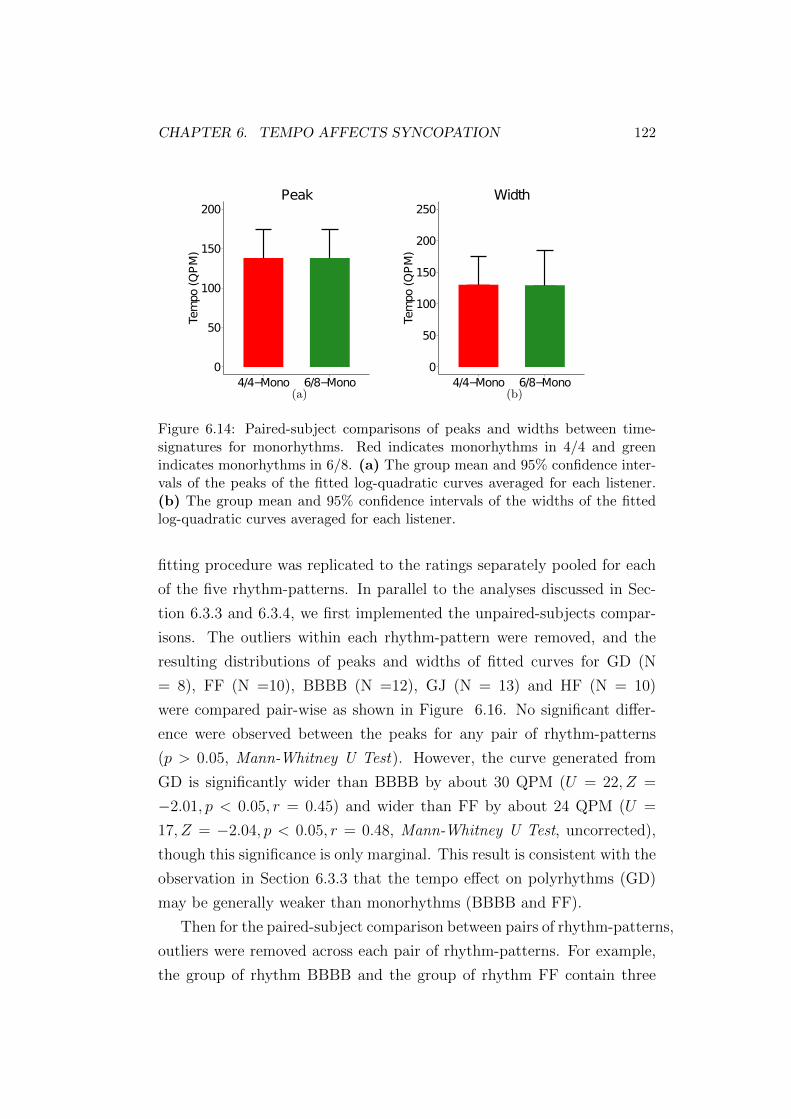
CHAPTER 6. TEMPO AFFECTS SYNCOPATION 122
0
50
100
150
200
4/4−Mono 6/8−Mono
Tempo
(QPM)
Peak
(a)
0
50
100
150
200
250
4/4−Mono 6/8−Mono
Tempo
(QPM)
Width
(b)
Figure 6.14: Paired-subject comparisons of peaks and widths between time-signatures for monorhythms. Red indicates monorhythms in 4/4 and greenindicates monorhythms in 6/8. (a) The group mean and 95% confidence inter-vals of the peaks of the fitted log-quadratic curves averaged for each listener.(b) The group mean and 95% confidence intervals of the widths of the fittedlog-quadratic curves averaged for each listener.
fitting procedure was replicated to the ratings separately pooled for each
of the five rhythm-patterns. In parallel to the analyses discussed in Sec-
tion 6.3.3 and 6.3.4, we first implemented the unpaired-subjects compar-
isons. The outliers within each rhythm-pattern were removed, and the
resulting distributions of peaks and widths of fitted curves for GD (N
= 8), FF (N =10), BBBB (N =12), GJ (N = 13) and HF (N = 10)
were compared pair-wise as shown in Figure 6.16. No significant differ-
ence were observed between the peaks for any pair of rhythm-patterns
(p > 0.05, Mann-Whitney U Test). However, the curve generated from
GD is significantly wider than BBBB by about 30 QPM (U = 22, Z =
−2.01, p < 0.05, r = 0.45) and wider than FF by about 24 QPM (U =
17, Z = −2.04, p < 0.05, r = 0.48, Mann-Whitney U Test, uncorrected),
though this significance is only marginal. This result is consistent with the
observation in Section 6.3.3 that the tempo effect on polyrhythms (GD)
may be generally weaker than monorhythms (BBBB and FF).
Then for the paired-subject comparison between pairs of rhythm-patterns,
outliers were removed across each pair of rhythm-patterns. For example,
the group of rhythm BBBB and the group of rhythm FF contain three

CHAPTER 6. TEMPO AFFECTS SYNCOPATION 123
BF
●
●●
● ●●
●●
0
1
2
3
4
30 60 120 240 480Tempo (QPM)
Rat
ing
(a)
GD *●
●
● ●●
● ●
●
0
1
2
3
4
30 60 120 240 480Tempo (QPM)
Rat
ing
(b)
AJ
●
●
●●
●
● ● ●
0
1
2
3
4
30 60 120 240 480Tempo (QPM)
Rat
ing
(c)
FF
*
●
●
●
●
●
●
●
●
0
1
2
3
4
30 60 120 240 480Tempo (QPM)
Rat
ing
(d)
GJ
*
● ●
●
●
● ●
●
●
0
1
2
3
4
30 60 120 240 480Tempo (QPM)
Rat
ing
(e)
HF
*●
●
●
● ● ● ●
●
0
1
2
3
4
30 60 120 240 480Tempo (QPM)
Rat
ing
(f)
BBBB
*●
●●
● ●●
●
●
0
1
2
3
4
30 60 120 240 480Tempo (QPM)
Rat
ing
(g)
DBDB
●
● ●● ●
●
●
●
0
1
2
3
4
30 60 120 240 480Tempo (QPM)
Rat
ing
(h)
Figure 6.15: Tempo effects between rhythm-patterns. The group means synco-pation ratings of each rhythm-pattern against tempi are plotted. The shadedareas indicate 95% confidence intervals. * denotes significance (p < 0.05,Friedman Rank Sum Test). The rhythms in the first row, (a)-(c), are 4/4polyrhythms; those in the second row, (d)-(f), are 6/8 monorhythms; and thosein the third row, (g) and (h), are 4/4 monorhythms. The coloured fitted log-quadratic curves were fitted and plotted for the rhythm-patterns that haveshown a significant tempo effect.
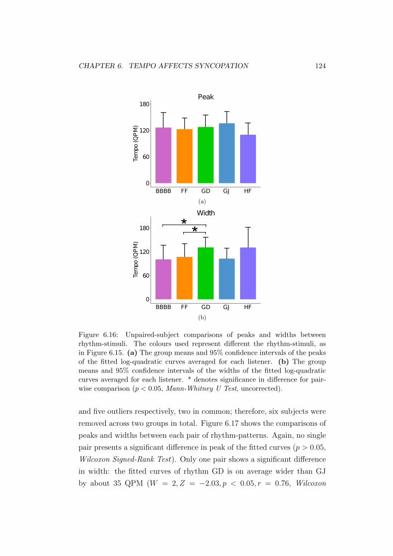
CHAPTER 6. TEMPO AFFECTS SYNCOPATION 124
0
60
120
180
BBBB FF GD GJ HF
Tempo
(QPM)
Peak
(a)
0
60
120
180
BBBB FF GD GJ HF
Tempo
(QPM)
Width
**
(b)
Figure 6.16: Unpaired-subject comparisons of peaks and widths betweenrhythm-stimuli. The colours used represent different the rhythm-stimuli, asin Figure 6.15. (a) The group means and 95% confidence intervals of the peaksof the fitted log-quadratic curves averaged for each listener. (b) The groupmeans and 95% confidence intervals of the widths of the fitted log-quadraticcurves averaged for each listener. * denotes significance in difference for pair-wise comparison (p < 0.05, Mann-Whitney U Test, uncorrected).
and five outliers respectively, two in common; therefore, six subjects were
removed across two groups in total. Figure 6.17 shows the comparisons of
peaks and widths between each pair of rhythm-patterns. Again, no single
pair presents a significant difference in peak of the fitted curves (p > 0.05,
Wilcoxon Signed-Rank Test). Only one pair shows a significant difference
in width: the fitted curves of rhythm GD is on average wider than GJ
by about 35 QPM (W = 2, Z = −2.03, p < 0.05, r = 0.76, Wilcoxon

CHAPTER 6. TEMPO AFFECTS SYNCOPATION 125
0
50
100
150
200
BBBB FF
BBBB GJ
BBBB
HF
BBBB
GD FF GJ
FF HF FF GD GJ
HF GJ
GD
HF
GD
Tempo
(QPM)
Peak
(a)
0
50
100
150
200
BBBB FF
BBBB GJ
BBBB
HF
BBBB
GD FF GJ
FF HF FF GD GJ
HF GJ
GD HF
GD
Tempo
(QPM)
Width
*
(b)
Figure 6.17: Paired-subject comparisons of peaks and widths between pairs ofrhythm-stimuli. The colours used represent different the rhythm-stimuli, as inFigure 6.15. (a) The group means and 95% confidence intervals of the peaks ofthe fitted log-quadratic curves averaged for each listener. (b) The group meansand 95% confidence intervals of the widths of the fitted log-quadratic curvesaveraged for each listener. * denotes significance in difference for pair-wisecomparison (p < 0.05, Wilcoxon Signed-Rank Test, uncorrected).
Signed-Rank Test, uncorrected).
An alternative paired-subject comparison requires removing outliers
across all five rhythm-patterns. Yet, this method suffers from too few
common subjects (N = 5) throughout entire rhythm-patterns, resulting in
too weak a power of the analysis. Therefore we choose not to implement

CHAPTER 6. TEMPO AFFECTS SYNCOPATION 126
it.
In summary, we observed a diversity of tempo effects on individual
rhythm-patterns. Syncopation elicited by rhythm-patterns BBBB, FF,
GD, GJ and HF is strongly affected by tempo, whereas the tempo ef-
fect on other rhythms was not significantly affected by tempo. The five
rhythm-patterns have similar estimated tempi that correspond to maxi-
mum syncopation, i.e. the peaks of fitted quadratic curves. However, the
tempo effect on GD seems to be significantly wider than BBBB, FF, and
GJ. This can be interpreted as further evidence supporting the theory that
syncopation aroused by polyrhythms is less sensitive to tempo changes.
6.4 Discussion
We collected ratings of syncopation perception for several syncopated
rhythm-patterns being transposed over a wide range of tempi. Overall,
the results confirm our hypothesis that the strength of syncopation per-
ception is maximised at middle range tempi and weakened towards the
extreme tempi (Figure 6.4). We have also found that monorhythms are
more strongly affected by tempo than polyrhythms (Figures 6.6 - 6.8).
The causes of these phenomena may be two-fold: tempo influences the
perception of tactus and tempo prompts the adjustment of tactus between
metrical levels. Our data show a weaker tempo effect on rhythms in 4/4
meter than 6/8 (Figures 6.9 - 6.11), but this may be mostly due to the
difference in tempo effects between polyrhythms and monorhythms, as
the 4/4 group is a mixture of monorhythms and polyrhythms but the 6/8
group only includes monorhythms. Indeed, after excluding polyrhythms
from the comparison there is no longer any evidence to suggest a significant
difference (Figures 6.12 - 6.14). Therefore, we can conclude that tempo
effect does not appear to differentiate between the time-signatures of 4/4
and 6/8.
Additionally, we found no substantial difference in the tempo effects
among individual rhythm-patterns (Figures 6.15 - 6.17). The marginally
significant difference in widths of fitted curves between GD and FF, be-
tween GD and BBBB (Figure 6.16), or between GD and GJ (Figure 6.17)

CHAPTER 6. TEMPO AFFECTS SYNCOPATION 127
can be interpreted as the difference in tempo effects between monorhythms
and polyrhythms. In Section 6.4.6, we provide possible explanations for
the observations that time-signature and rhythm-patterns do not have an
effect.
6.4.1 The tempo effect on syncopation parallels the tempo ef-
fect on tactus
Based on the evidence reviewed in Section 6.1.1 and 6.1.2, the range of
beat rates known to afford a perception of tactus is approximately from
200 ms to 2000 ms (30 - 300 BPM) [Lon04]. The overall probability
function of beat-tapping rates roughly yields a normal distribution on a
logarithmic-scale of tempo [Par94, Moe02]. The preference of tapping
rates may reflect the perceptual strengths of beat salience [Fra82, Moe02].
In this case, the perception of beat should be maximised at a moderate
range of tempi (500 - 750 ms, 80 - 120 BPM), and decay towards the
boundaries of tactus perception.
Syncopation is the product of rhythm foreground contradicting the
metrical background. When the beat is weakly perceived (or even not
perceivable), then it cannot serve as the background for the contradic-
tion that arouses the perception of syncopation. This could help with
explaining the observed log-quadratic relationship between syncopation
and tempo, which appears similar to the relationship between tactus per-
ception and tempo.
To be more specific, when the metronome is presented at 30 BPM,
which is the lower limit of tactus perception (2000 ms), listeners will have
difficulty in hearing successive beats as a continuous stream [Fra82]. In-
stead, the beats are perceived as unconnected events, imposed onto the
rhythmic events. In this case, it is possible that listeners no longer hear
the rhythm and metronome as two streams that interact with each other,
but rather one sequence of unrelated events.
As the metronome speeds up, the perceptual strength of beat salience
increases, hence the perception of metrical background is better formed.
As a result, the contradiction between rhythm and meter becomes more

CHAPTER 6. TEMPO AFFECTS SYNCOPATION 128
evident, leading to a stronger perception of syncopation.
At very fast tempi (e.g. 360 and 480 BPM in Figure 6.4), the rates of
metronome ticks are beyond the upper limit of tactus perception (about
200 ms, 300 BPM), and are getting close to the limits of meter percep-
tion (about 100 ms, 600 BPM). Then, the metronome is too fast to be
perceivable as a tactus, whereas rhythm-patterns that possess longer inter-
onset intervals than the metronome can still be perceived. Two streams of
events, metronome and rhythm, are rendered as different sounds. This al-
lows listeners to segregate the metronome events from the rhythm events.
However, when the metronome becomes too fast to be perceived, it effec-
tively turns into noise, being superimposed onto the perceivable rhythm.
Then, it is possible that listeners are inclined to only process the infor-
mation in the rhythms and ignore this noise. As a result, the perception
of syncopation will be weakened because listeners are no longer hearing
the contradiction between rhythms and meter, but may either interpret
different meter induced by the rhythm [Lon04] or may process rhythms
in a nonmetric way, i.e. the rhythm interpretation strategy that does not
involve extracting periodic pulses from the rhythms [HL83].
In short, the effect of tempo on the perception of syncopation can be
explained by the known effects of tempo on tactus perception. The ex-
treme slow or fast tempi undermine the perception of tactus, on which
the perception of syncopation depends. While this explains the general
shape of tempo effect on syncopation, it cannot explain why the curve of
the tempo effect on tactus perception does not fully coincide with that of
syncopation. In the following sections, we attempt to provide an explana-
tion for this based on the findings of other studies that show that tempo
influences the adjustment of tactus in between metrical levels.
6.4.2 Adjustable tactus level and syncopation
In Section 6.1.3, we introduced the phenomenon of shifting tactus between
metrical levels to adapt to the change in tempo. To maintain the beat-
intervals of tactus in a preferred range, listeners tend to move it to lower
metrical levels when the tempo (of the defined beat level) is too slow, or

CHAPTER 6. TEMPO AFFECTS SYNCOPATION 129
move it to higher metrical levels if the tempo is too fast. Some evidence
suggests that the selection of tactus level is centred around a beat interval
of 100 BPM (600 ms) [HSEK04, Fra82]; others suggest a range of 60 - 120
BPM (500 - 1000 ms ) [Duk89] or 75 - 300 BPM (200 - 800 ms) [HO81].
As Cooper and Meyer hypothesised (Section 6.1.4), the adjustment
of tactus level may directly affect the perception of syncopation. For
monorhythmic patterns (e.g. BBBB, FF) at 30 QPM, listeners may per-
ceive tactus at a lower rhythmic level than the beat level of metronome
by interpolating beats. In consequence, some notes that were supposed to
be off-beat become on-beat, hence the syncopation is diminished. At the
other end of the tempo scale, when beat rates exceed 120 QPM, listeners
may shift tactus to a higher metrical level by effectively ‘under-sampling’
the metronome ticks. Therefore some notes that were originally on-beat
become off-beat, resulting in syncopation.
6.4.3 Peak tempo of syncopation is lagged to that of tactus
The theory of adjusting tactus level with change in tempo may further
explain why the tempo that corresponds to the maximal syncopation (180
- 240 QPM, Figure 6.4) is faster than the peak tempo for tactus perception
(varying from 80 to 120 BPM, Section 6.1.1) ,and the slightly asymmetrical
shape of the log-tempo curve. When tempo exceeds the upper limit of
preferred tactus rates, the tactus rate moves back to the preferred range by
adjusting the tactus level. This causes the perceptual strength of tactus to
decrease with the increasing tempo, but meanwhile syncopation increases
due to the adjustment of tactus level. This tendency may continue until
tempo becomes too fast to allow the adjustment of tactus level.
6.4.4 Polyrhythms versus monorhythms
Syncopation elicited by polyrhythms is less affected by tempo than monorhythms
(Section 6.3.3, Figure 6.6). For polyhrhythms, but not monorhythms,
shifting tactus to a lower metrical level at slow tempi could not reduce
the contradiction between the polyrhythm and meter. This is because the
nature of polyrhythms is to produce a constant mismatch between rhythm

CHAPTER 6. TEMPO AFFECTS SYNCOPATION 130
and meter at any tempo because polyrhythms contain dissonant period-
icities [HO81, Yes76]. Therefore in polyrhythms, some notes can never
coincide with the metrical positions at any beat level and hence there will
always be a contradiction to the meter.
Nevertheless, polyrhythms still exhibit a mild tendency of diminished
syncopation towards extreme tempi, which may be due to the decreasing
strength of meter perception in general (Section 6.4.1). Handel tested the
relationship between rhythm discrimination and tempo, and found that
the same patterns played at different tempi were perceived as different
rhythms [Han93]. Perhaps at extreme tempi, listeners have more difficulty
in precisely judging the inter-relationships between notes in polyrhythms
compared to patterns played at moderate tempi. It is possible that the
affected timing structure between notes also changes the relationship be-
tween rhythm and meter, making it less contradictory.
6.4.5 Possible meter induction at extremely fast tempi
In Section 6.4.1, we suggested that at extremely fast tempi, rhythm-
patterns may be separately processed from the noise-like metronome.
These rhythm-patterns may induce a different metrical interpretation for
the judgement of syncopation. Interestingly, we found that the syncopa-
tion of rhythms BBBB, GJ and FF decrease more steeply than HF after
peak tempi (roughly 180 - 240 QPM, Figure 6.15). These three rhythms all
contain evenly spaced notes (Figure 6.3), which are more likely to induce
periodic beats that align with the notes [PE85]. In contrast, the notes
in rhythm HF are not evenly distributed. Therefore, it is plausible that
the syncopation perception of rhythms BBBB, GJ and FF decreases more
quickly at fast tempi because they naturally induce a meter that fits well
with the rhythm-patterns, and hence are perceived as less syncopated.
6.4.6 Time-signature
For monorhtyhms, the peak tempi and the widths for the fitted curves are
more or less the same for different time-signatures and individual rhythm-
patterns (Figure 6.12b and 6.15). Although these monorhythms may elicit
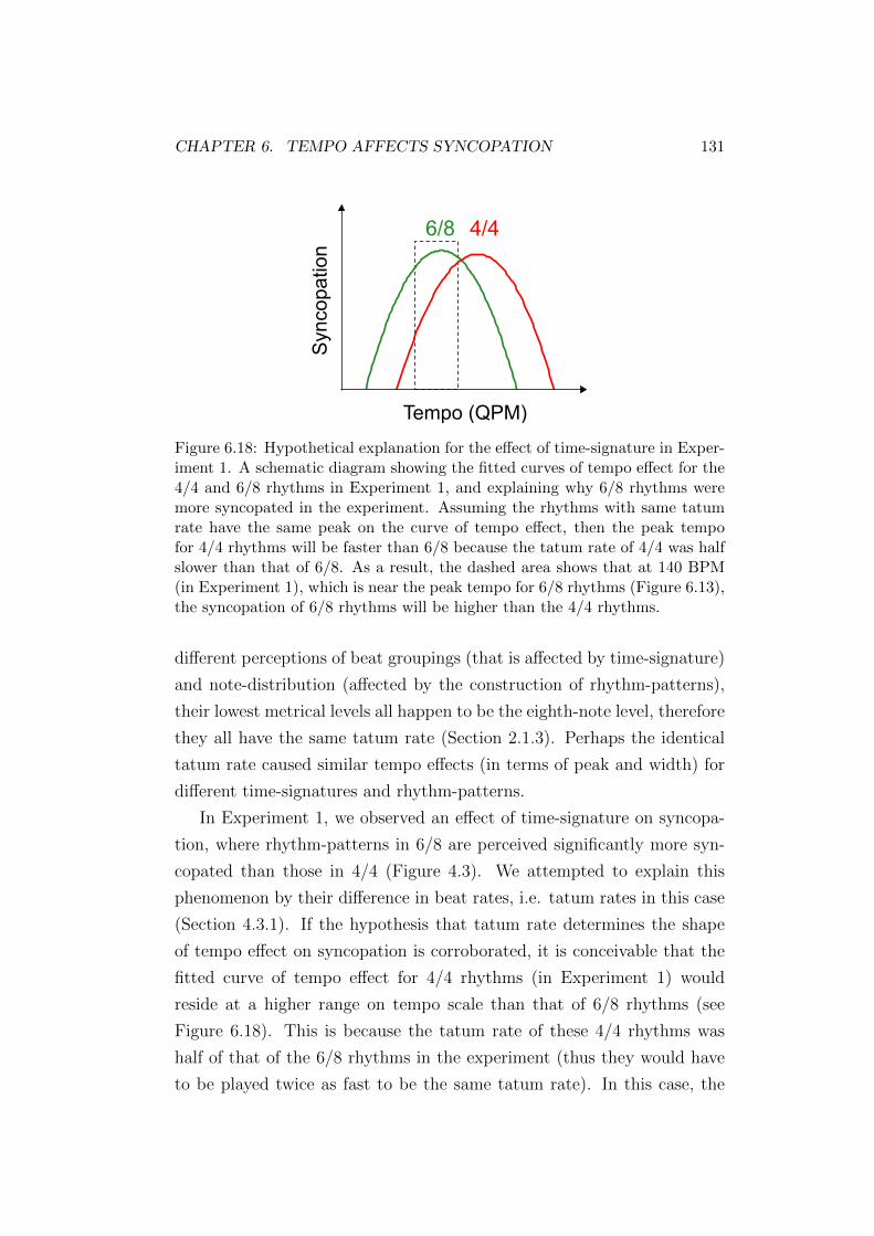
CHAPTER 6. TEMPO AFFECTS SYNCOPATION 131
Tempo (QPM)
Syn
co
pa
tio
n
6/8 4/4
Figure 6.18: Hypothetical explanation for the effect of time-signature in Exper-iment 1. A schematic diagram showing the fitted curves of tempo effect for the4/4 and 6/8 rhythms in Experiment 1, and explaining why 6/8 rhythms weremore syncopated in the experiment. Assuming the rhythms with same tatumrate have the same peak on the curve of tempo effect, then the peak tempofor 4/4 rhythms will be faster than 6/8 because the tatum rate of 4/4 was halfslower than that of 6/8. As a result, the dashed area shows that at 140 BPM(in Experiment 1), which is near the peak tempo for 6/8 rhythms (Figure 6.13),the syncopation of 6/8 rhythms will be higher than the 4/4 rhythms.
different perceptions of beat groupings (that is affected by time-signature)
and note-distribution (affected by the construction of rhythm-patterns),
their lowest metrical levels all happen to be the eighth-note level, therefore
they all have the same tatum rate (Section 2.1.3). Perhaps the identical
tatum rate caused similar tempo effects (in terms of peak and width) for
different time-signatures and rhythm-patterns.
In Experiment 1, we observed an effect of time-signature on syncopa-
tion, where rhythm-patterns in 6/8 are perceived significantly more syn-
copated than those in 4/4 (Figure 4.3). We attempted to explain this
phenomenon by their difference in beat rates, i.e. tatum rates in this case
(Section 4.3.1). If the hypothesis that tatum rate determines the shape
of tempo effect on syncopation is corroborated, it is conceivable that the
fitted curve of tempo effect for 4/4 rhythms (in Experiment 1) would
reside at a higher range on tempo scale than that of 6/8 rhythms (see
Figure 6.18). This is because the tatum rate of these 4/4 rhythms was
half of that of the 6/8 rhythms in the experiment (thus they would have
to be played twice as fast to be the same tatum rate). In this case, the

CHAPTER 6. TEMPO AFFECTS SYNCOPATION 132
syncopation of 6/8 rhythms would therefore be higher than 4/4 because
the former has reached maxima at peak tempo but the latter has not (e.g.
the dashed area shown in Figure 6.18). However, this speculation requires
further investigation into how the syncopation perception of 4/4 rhythms
in Experiment 1 varies with change in tempo.
6.5 Summary
In this chapter, we have evaluated the relationship between tempo and
perceived syncopation by manipulating the tempo of rhythm-patterns that
were known to give rise to syncopation in Experiment 1. Listeners were
asked to rate the degree of syncopation they perceived in response to a
rendering of each of 64 rhythm-stimuli (e.g. eight rhythm-patterns ×eight tempi). Our main hypothesis that the perception of syncopation is a
function of tempo is confirmed, and such relationship can be well-captured
by a log-quadratic function. We also found that the tempo effect on
monorhythms is significantly stronger than that on polyrhythms. Yet, no
clear evidence was found to suggest a difference in tempo effects between
time-signatures and between rhythm-patterns.
Our observations appear to be related to the known effects of tempo
on tactus perception and meter perception. A weakened sense of beat and
meter at very slow and very fast tempi may simultaneously reduce the
contradiction between rhythm and meter, and hence lead to less synco-
pation. The theory that listeners naturally adjust tactus level to retain a
‘comfort’ tactus rate could explain why the peak tempo for syncopation
is higher than that of tactus, and why polyrhythms are more resistant to
tempo than monorhythms. We also suggest a possible meter induction
from rhythm-patterns over the non-processable metronome, which could
explain some rhythms that are more likely to induce a meter are perceived
as less syncopated at fast tempi than those are not. Finally, the similar
tempo effects between time-signatures and rhythm-patterns might be the
result of the identical tatum rate of all the monorhythms.
The study in this chapter not only presents evidence for some theoreti-
cal speculations of the relationship between tempo and syncopation [CM60],

CHAPTER 6. TEMPO AFFECTS SYNCOPATION 133
but also provides new insight into syncopation modelling that is tempo-
dependent. In the next chapter, to suggest the ways in which the models
may be improved, we combine the findings from evaluation results of ex-
isting syncopation models (Chapter 5) to select the best model(s), and
the curves characterising the tempo effects on syncopation that we found
in this chapter.
Chapter 7
Improving syncopation modelling
The evaluation results of existing syncopation models against Dataset 1
presented in Chapter 5 suggest that no single model can predict this en-
tire dataset well, and there is still much room for improvement for 6/8
monorhythms and polyrhythms. In this chapter, we explore ways to im-
prove current syncopation modelling. Having highlighted the strengths
and weaknesses of the various modelling architectures in Section 5.3, and
considering the limited scope of each model, it would appear that the most
immediate solution to predicting the data as a whole is a combination of
the models.
In Sections 7.1 and 7.2, we introduce three combined models, all of
which adopt techniques of linear regression to seek better fits to Dataset
1. These combined models requires identification of time-signature and
discrimination of rhythm-categories. We then validate them with Dataset
1, compare them with the individual existing syncopation models and
with each other in Section 7.3. Based on that, we attempt to incorpo-
rate the tempo-dependent nature of syncopation found in Experiment 2
to syncopation modelling, and extend the three combined models to cap-
ture Dataset 2. Finally, we validate these three tempo-dependent models
against Dataset 2 and the combination of two datasets in Section 7.5.
7.1 Best-Single Combined models (BSC)
The simplest implementation of a combined model is to select the (single)
model best suited to predicting the particular subset of rhythms that lies
within their scope, then conditionally combine them.
134

CHAPTER 7. IMPROVING SYNCOPATION MODELLING 135
PRS WNBD Intercept
4/4 Mono 0.07*6/8 Mono 0.14* -0.304/4 Poly 0.24* 2.42*
Table 7.1: Linear regression coefficients for the BSC model.
* denotes significance (p < 0.05).
7.1.1 The three-way BSC model (BSC3)
The predictions of individual syncopation models against human ratings
from Dataset 1 were plotted in Figures 5.4 - 5.6. Pressing’s model (PRS)
is the optimal candidate for both 4/4 monorhythms (r = 0.95, p < 0.001)
and 6/8 monorhythms (r = 0.76, p < 0.001), and the WNBD model is
optimal for polyrhythms (r = 0.41, p < 0.001).
Table 7.1 shows all the coefficients estimated by least-square regression
to get the best fit to each subset. The equation for the combination of
this three-way BSC models is as follows:
SBSC3(Y ) =
0.07SPRS(Y ), if 4/4 monorhythms;
0.14SPRS(Y )− 0.3, if 6/8 monorhythms;
0.24SWNBD(Y ) + 2.42, if polyrhythms.
(7.1)
where SPRS and SWNBD were defined in Equations 3.29 and 3.52 respec-
tively.
7.1.2 The two-way BSC model (BSC2)
Alternatively, since the PRS model showed the best performance for monorhythms
in both time-signatures, we can divide the entire dataset into two sub-
categories: monorhythms and polyrhythms, then combine the predictions
of PRS model for monorhythms and predictions of WNBD model for
polyrhythms to capture all.
Table 7.2 shows the coefficients estimated by least-square regression to
get the best fit to each of the two subsets of the data. The equation for
the two-way BSC model is as follows:
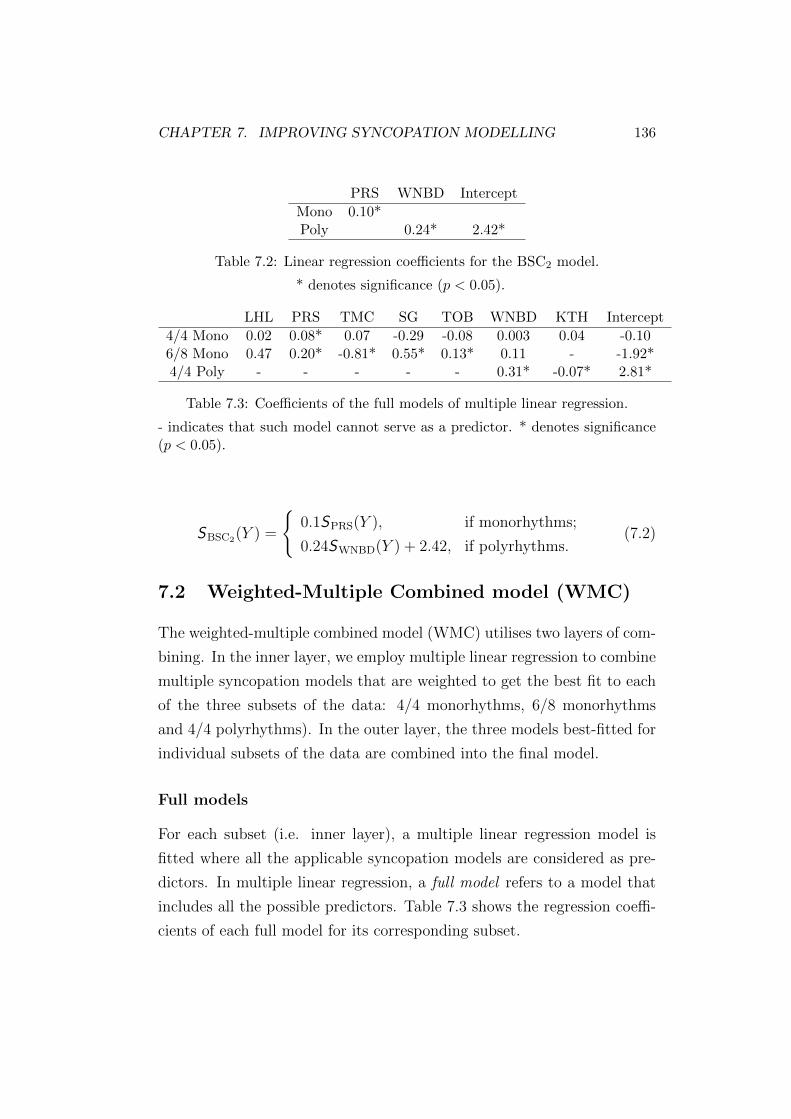
CHAPTER 7. IMPROVING SYNCOPATION MODELLING 136
PRS WNBD Intercept
Mono 0.10*Poly 0.24* 2.42*
Table 7.2: Linear regression coefficients for the BSC2 model.
* denotes significance (p < 0.05).
LHL PRS TMC SG TOB WNBD KTH Intercept
4/4 Mono 0.02 0.08* 0.07 -0.29 -0.08 0.003 0.04 -0.106/8 Mono 0.47 0.20* -0.81* 0.55* 0.13* 0.11 - -1.92*4/4 Poly - - - - - 0.31* -0.07* 2.81*
Table 7.3: Coefficients of the full models of multiple linear regression.
- indicates that such model cannot serve as a predictor. * denotes significance(p < 0.05).
SBSC2(Y ) =
{0.1SPRS(Y ), if monorhythms;
0.24SWNBD(Y ) + 2.42, if polyrhythms.(7.2)
7.2 Weighted-Multiple Combined model (WMC)
The weighted-multiple combined model (WMC) utilises two layers of com-
bining. In the inner layer, we employ multiple linear regression to combine
multiple syncopation models that are weighted to get the best fit to each
of the three subsets of the data: 4/4 monorhythms, 6/8 monorhythms
and 4/4 polyrhythms). In the outer layer, the three models best-fitted for
individual subsets of the data are combined into the final model.
Full models
For each subset (i.e. inner layer), a multiple linear regression model is
fitted where all the applicable syncopation models are considered as pre-
dictors. In multiple linear regression, a full model refers to a model that
includes all the possible predictors. Table 7.3 shows the regression coeffi-
cients of each full model for its corresponding subset.

CHAPTER 7. IMPROVING SYNCOPATION MODELLING 137
Reduced models
A full model may contain a large amount of predictors and some of them
may be redundant (i.e. the predictors that are not significant or are given
with small coefficients so that they effectively did not add much to the
model). We then adopt stepwise regression procedure [Mil90] to select
the best set of predictors while retaining a good predictive ability. The
resulting model that contains a subset of predictors in a full model is
referred as a reduced model.
For each subset, we tested two common approaches for stepwise re-
gression, forward selection and backward elimination [Mil90], to select the
most suitable method. The forward selection procedure starts with no
predictor in the model and incrementally adds predictors until there are
no further improvement of the model. In contrast, backward elimination
starts with a full model and gradually removes predictors while keeping
the same level of performance. The criterion for predictor selection we
used is the bayesian information criterion [Aka77], which is designed to
balance the performance and the complexity of the model. To be more
specific, this criterion tries to optimise goodness of fit of the model while
retaining the minimum number of free parameters to avoid over-fitting.
Forward selection and backward elimination produce identical results
for 6/8 monorhythms (R2 = 68.0%, F (4, 31) = 19.58, p < 0.001), and
for 4/4 polyrhythms (R2 = 22.2%, F (2, 45) = 7.69, p < 0.01). However,
forward selection shows a slight advantage over backward elimination for
4/4 monorhythms (forward selection, R2 = 87.7%, F (3, 23) = 62.87, p <
0.001; backward elimination, R2 = 86.6%, F (2, 24) = 85.16, p < 0.001).
We therefore adopt the set of predictors optimised by forward stepwise
regression for each subsets. The updated coefficients of the reduced models
for each subset are shown in Table 7.4.
In the outer layer, the combination of the full models and the combina-
tion of the reduced models have shown basically equal-well performance,
(full model, r = 0.90, R2 = 85.1%, F (1, 109) = 627.8, p < 0.001; reduced
model, r = 0.89, R2 = 84.6%, F (1, 109) = 603.2, p < 0.001), but the re-
duced models for subsets of 4/4 monorhythms and 6/8 monorhythms are

CHAPTER 7. IMPROVING SYNCOPATION MODELLING 138
LHL PRS TMC SG TOB WNBD KTH Intercept
4/4 Mono 0.05* 0.09* -0.08* -0.116/8 Mono 0.17* -0.22* 0.67* 0.11* - -1.19*4/4 Poly - - - - - 0.31* -0.07* 2.81*
Table 7.4: Coefficients of the reduced models of multiple linear regression.
- indicates that such model cannot serve as a predictor. * denotes significance(p < 0.05).
much simplified than the corresponding full models. We therefore choose
the combination of the reduced models to be the final WMC model, re-
sulting in the following equation:
SWMC(Y ) =
0.05SLHL(Y ) + 0.09SPRS(Y )− 0.08STOB(Y )− 0.11,
if 4/4 monorhythms;
0.17SPRS(Y )− 0.22STMC(Y ) + 0.67SSG(Y ) + 0.11STOB(Y )− 1.19,
if 6/8 monorhythms;
0.31SWNBD(Y )− 0.07SKTH(Y ) + 2.81,
if polyrhythms.
(7.3)
where the equations of individual syncopation models refer back to Sec-
tion 3.2
7.3 Validation of combined models for Dataset 1
Among individual syncopation models, only the WNBD (Equation 3.52)
and TOB models (Equation 3.47) are able to predict the entire Dataset
1. Figure 7.1 plots the predictions of these two models and the three
new combined models, BSC2 (Equation 7.2), BSC3 (Equation 7.1) and
the WMC model (Equation 7.3) against Dataset 1 for comparison.
All three combined models showed a marked improvement over the
WNBD and TOB models (BSC2, r = 0.85, p < 0.001; BSC3, r = 0.87, p <
0.001; WMC, r = 0.89, p < 0.001; WNBD, r = 0.44, p < 0.001; TOB,
r = −0.54, p < 0.001, Spearman’s Rank Correlation). This suggests that
the combined modelling architecture is effective.
The two-way BSC model (BSC2, r = 0.85, R2 = 74.9%, F (1, 109) =

CHAPTER 7. IMPROVING SYNCOPATION MODELLING 139
r = −0.54p< 0.001
0
.25
.5
.75
1
0 .25 .5 .75 1Human Rating
Pre
dict
ion
ST
OB
(a)
r = 0.44p< 0.001
0
.25
.5
.75
1
0 .25 .5 .75 1Human Rating
Pre
dict
ion
SW
NB
D(b)
r = 0.87p < 0.001
0
.25
.5
.75
1
0 .25 .5 .75 1Human Rating
Pre
dict
ion
SB
SC
3
(c)
r = 0.85p < 0.001
0
.25
.5
.75
1
0 .25 .5 .75 1Human Rating
Pre
dict
ion
SB
SC
2
(d)
r = 0.89p < 0.001
0
.25
.5
.75
1
0 .25 .5 .75 1Human Rating
Pre
dict
ion
SW
MC
(e)
Figure 7.1: Predictions of combined models for Dataset 1. The normalisedpredictions are plotted against the normalised mean human ratings. Red datapoints indicate 4/4 monorhythms, blue indicates 6/8 monorhythms and greenindicates 4/4 polyrhythms. Spearman-rank correlation coefficients (r,p) aregiven for each model. Linear regression lines (and 95% confidence interval) areplotted for illustration.

CHAPTER 7. IMPROVING SYNCOPATION MODELLING 140
327.4, p < 0.001) does not perform as well as the three-way BSC model
(BSC3, r = 0.87, R2 = 80.0%, F (1, 109) = 443.5, p < 0.001). This is prob-
ably because the BSC2 model is under-fitted by a singular linear regression
model when trying to accommodate two subsets at the same time. In con-
trast, the BSC3 model generates fewer errors because it uses two separate
models to capture subset.
The WMC model (WMC, r = 0.89, R2 = 84.6%, F (1, 109) = 603.2, p <
0.001) performs better than any of the BSC models. This is not surprising
because multiple regression features a greater number of free parameters,
which on the other hand is likely to cause overfitting.
7.4 Tempo-dependent models
One of the major findings in Experiment 2 is that tempo has a strong effect
on syncopation, and the relationship between syncopation and tempo can
be characterised by a log-quadratic function (Figure 6.4). However, this
has not been considered by any of the existing syncopation models. In
this section, we propose an extension to any syncopation model to allow
it to be tempo-dependent.
7.4.1 General design
Figure 7.2 gives a schematic showing the addition of tempo-dependence
to an existing syncopation model M, forming the tempo-dependent model
M∼ T. Crucially, we assume the prediction given by this syncopation
model corresponds to the maximum syncopation value at peak tempo.
Also, we restrict the tempo to be within the range from 30 to 480 QPM.
7.4.2 Tempo-dependent combined models
In Experiment 2, we found that the fitted curves for mean ratings of
polyrhythms are significantly wider than those for mean ratings of monorhythms
(Figures 6.6 - 6.8, Section 6.3.3). This suggests that when applying tempo-
dependent scaling to syncopation models, monorhythms and polyrhythms

CHAPTER 7. IMPROVING SYNCOPATION MODELLING 141
Rhythm
Figure 7.2: A tempo-dependent model. A schematic diagram showing that atempo-dependent model M∼T is generated by applying a tempo-dependentscaling function F to an existing syncopation model M, providing the finalprediction of syncopation for a rhythm.
need separate scaling functions. Here, we use Fm and Fp to represent the
scaling function for monorhythms and polyrhythms respectively.
The flow chart in Figure 7.3 shows the overall algorithm for tempo-
dependent combined models. For example, the syncopation value of a
monorhythm in 4/4 is calculated by the first sub-equation in Equation 7.1,
and then scaled by scaling function of monorhythms Fm to generate the
final syncopation prediction of BSC3∼T model.
The tempo-dependent scaling functions serve the purpose of moder-
ating syncopation at any tempo in relation to the maximum syncopa-
tion at peak tempo, consistent with the observed tempo effect on syn-
copation in Experiment 2. They are therefore generated by normalising
the log-quadratic functions fitted to the mean ratings of monorhythms
and polyrhythms (Figure 7.4), resulting in the following equations, where
tempo Υ ∈ [30, 480]:
Fm(Υ) = −0.22 ln2(Υ) + 2.18 ln(Υ)− 4.39 (7.4)
Fp(Υ) = −0.08 ln2(Υ) + 0.86 ln Υ− 1.20 (7.5)
Based on the above scaling functions, we can define the equation for
M ∼ T model by multiplying the equation for M model with tempo-
dependent scaling functions. For example, the equation for WMC∼ T
model is as follows:

CHAPTER 7. IMPROVING SYNCOPATION MODELLING 142
Rhythm
(pattern, time-signature and tempo)
mono?
4/4?
Figure 7.3: Flow chart of the overall algorithm for tempo-dependent combinedmodels.
SWMC∼T(Y,Υ) =
{SWMC(Y )Fm(Υ), if monorhythms;
SWMC(Y )Fp(Υ), if polyrhtyhms;(7.6)
7.5 Validation of tempo-dependent combined mod-
els for Dataset 2
In this section, we validate the three tempo-dependent combined models,
BSC2∼T, BSC3∼T and WMC∼T, against Dataset 2. For each tempo-
dependent combined model, the prediction of the model for a given stim-
ulus at certain tempo was compared to the mean of the human ratings for
that stimulus at the same tempo. The human ratings are not normally
distributed, therefore we have calculated the Spearman’s rank correlation
coefficient between each model and perceptual data.
Figure 7.5 plots the predictions of the models as a function of the

CHAPTER 7. IMPROVING SYNCOPATION MODELLING 143
1
1.5
2
2.5
3
30 60 120 240 480
Tempo (QPM)
Rating
(140, 2.17)
(165, 3.02)
0
.5
1
30 60 120 240 480
.75
.25
30 60 120 240 480Tempo (QPM)
0
.5
1
.75
.25
Tempo (QPM)
Normalise
Normalise
Fp(t)
Fm(t)
Figure 7.4: Separate tempo scaling functions for monorhythms andpolyrhythms. Based on the quadratic functions fitted to the mean ratings ofpolyrhythms (purple) and monorhythms (red) given in Figure 6.6, we normalisethese two curves (by their maxima), which turns into the scaling functions Fpfor polyrhythms, and Fm for monorhythms of tempo Υ.
perceptual data, including the regression line (±95% confidence inter-
vals). The BSC3∼T model performed remarkably better than the oth-
ers (r = 0.89, R2 = 69.6%, F (1, 62) = 145, p < 0.001); the BSC2 ∼T model shows advantage over the WMC ∼ T model (BSC2 ∼ T, r =
0.78, R2 = 61.0%, F (1, 62) = 99.71, p < 0.001; WMC∼T, r = 0.75, R2 =
45.9%, F (1, 62) = 54.38, p < 0.001).
In parallel to the validation result for Dataset 1, where the BSC3 model
performs better than the BSC2 model (Figure 7.1), the BSC3∼T model
also performs better in predicting Dataset 2 than the BSC2∼T model, and
shows an even more obvious advantage. This may mean that BSC2 model
is indeed under-fitted to Dataset 1, and the application of the tempo-
dependent scaling functions to BSC2 have amplified this error.
Another interesting finding is that after applying tempo-dependent
scaling to the combined models, the WMC model did not continue to
retain the advantage over the BSC models in predicting Dataset 1 (Fig-
ure 7.1c-d), but performed a lot worse in predicting Dataset 2, especially

CHAPTER 7. IMPROVING SYNCOPATION MODELLING 144
r =0.89p<0.001
1
2
3
1 2 3Human Rating
PredictionSBSC3~T
(a)
r =0.78p<0.001
1
2
3
1 2 3Human Rating
PredictionSBSC2~T
(b)
r =0.75p<0.001
1
2
3
1 2 3Human Rating
PredictionSWMC~T
(c)
Figure 7.5: Predictions of tempo-dependent combined models for Dataset 2.The predictions of each model are plotted against mean human ratings. Reddata points indicate 4/4 monorhythms, blue indicates 6/8 monorhythms andgreen indicates 4/4 polyrhythms. Spearman-rank correlation coefficients (r,p)are given for each model. Linear regression lines (and 95% confidence interval)are plotted for illustration.
than the three-way BSC model (Figure 7.5). This further suggests that the
multiple combined model is over-fitted to the data from Dataset 1, hence
it does not generalise syncopation modelling to a data from a different
paradigm (e.g. Dataset 2) and possibly a different sample of participants.
To this end, the single combined model seems to be more robust than the
multiple combined model.

CHAPTER 7. IMPROVING SYNCOPATION MODELLING 145
We have also tested the performance of all the combined models with-
out tempo adjustment (Equation 7.1 7.3) in predicting Dataset 2. The
percentage of explained variance (R2) drops 32.7% on average compar-
ing to the tempo-dependent combined models (BSC3, r = 0.74, R2 =
35.6%, F (1, 62) = 35.82, p < 0.001; BSC2 , r = 0.47, R2 = 28.6%, F (1, 62) =
26.2, p < 0.001; WMC, r = 0.43, R2 = 14.1%, F (1, 62) = 11.32, p < 0.01).
This demonstrates that the tempo-adjustment in combined models is ef-
fective in capturing Dataset 2.
7.6 Discussion
Generally, the combined modelling architecture has shown to be effective
in predicting Dataset 1. By adding the tempo-dependence extension to
this architecture, Dataset 2 is also well-captured. However, this approach
does not directly refine the theory for modelling syncopation, instead, it
searches for the best combinations of the elements in different models that
optimise the fit to the data. It also points out two potential directions
toward a more comprehensive mathematical model of syncopation: the
first is to extend the best performing hierarchical models (e.g. PRS model)
to capture polyrhythms and the second is to adapt the off-beat models to
take metrical hierarchy into account.
In addition, the combined modelling architecture is also more difficult
to interpret than an architecture with a single model representing a certain
hypothesis. This is because the multiple parameters in the combined
model need to be individually interpreted.
Another inherent limitation of the combined models is that by trained
only to fit Dataset 1, they do not necessarily provide an equivalent im-
provement for predictions on different rhythms. For example, other time-
signatures (that differ to 4/4 and 6/8) and different types of polyrhythms
(other than 2:3 polyrhythms) may not be well predicted. In other words,
these combined models may not be generalised enough to capture other
aspects in rhythm that can contribute to syncopation. Therefore, the
combined models require validation with datasets that these models are
not fitted to.

CHAPTER 7. IMPROVING SYNCOPATION MODELLING 146
To incorporate the tempo-dependence into syncopation models, we
adopted log-quadratic regression model to generate the tempo-dependent
scaling functions. Despite of the fact that this scaling function is simple
and easy to interpret, fittings of tempo-dependent models to Dataset 2
may be further improved by optimising the scaling functions to capture
Dataset 2. For example, we can extend Dataset 2 (which requires testing
syncopation in more tempi conditions) and optimise the log-quadratic re-
gression to a larger dataset; or we can try adopting different models (e.g.
Gaussian regression or high-order polynomial regression) to the current
Dataset 2.
7.7 Summary
In this chapter, we have provided two effective remedies to improve the
current approaches for modelling syncopation. The first remedy is to
combine the existing syncopation models that best suited to model each
subset of the data. Three new combined models are generated, validated
and all show good predictabilities. The second remedy is to apply tempo-
dependent scaling functions which capture the tempo effects on syncopa-
tion found in Experiment 2, to syncopation models to make them tempo-
dependent.
Generally, the new combined models, themselves and with the exten-
sion of tempo-dependence built in, can both capture the perception of
syncopation better than the current state of the art. However, having
highlighted their inherent limitations, these combined models require more
validation with new datasets that incorporate broader aspects of rhythm.

Chapter 8
Conclusions
In this thesis our objective was to investigate the theory and perception
of syncopation. We have reviewed the literature on the subject and gath-
ered the current models together by introducing a unified mathematical
framework. In order to test how well the theory and models explain the
perception of syncopation we have conducted two main experiments to
collect subjective ratings on perceived syncopation from musicians in re-
sponse to rhythm-stimuli. Using the findings from these experiments, we
have evaluated the previously existing models and built several new ones
that capture the perception of syncopation better than the current state
of the art.
8.1 Thesis contributions
This thesis makes a number of contributions to the understanding of syn-
copation both in terms of theory and perception. We have introduced new
methods for collecting perceptual syncopation ratings and produced two
new datasets using those methods.
Theory
We have reviewed various definitions and theories of syncopation in the
existing literature and summarised them into four main schools of thought
in Section 2.2. We have also examined seven existing models for syncopa-
tion, categorising their hypotheses, and consolidated them into a unified
147

CHAPTER 8. CONCLUSIONS 148
mathematical framework. Based on this mathematical framework, we
have implemented a syncopation model tool kit in Python [Son14].
We have evaluated the models against perceptual data from Dataset 1,
and discussed the relative strengths and weaknesses of each model. Using
these results, we have produced new combined models which out-perform
the previously existing ones.
We have extended the theory by providing evidence to show that syn-
copation is a function of tempo. Using this observed relationship, we have
extended our combined models so that they capture the tempo-dependent
nature of syncopation.
Method
We have conducted two experiments that investigate the perception of
syncopation using psychophysical methods. In contrast to previous stud-
ies, our experiment provides the first direct investigation on the perception
of syncopation.
Data
We have collected two psychophysical datasets that include perceptual
ratings of syncopation from trained musicians [Son14]. These datasets
have been used to evaluate the existing models in this work. They can
also be used in future studies that investigate a broad range of correlates
of syncopation in multiple disciplines.
8.2 General discussion
In this section, we unify the theory on syncopation and the findings from
our perceptual studies, and discuss what are the aspects captured in the
theory, what are the aspects mentioned in the theory but not verified, and
what are the missing elements in the theory.
All the theories share the consensus that syncopation is aroused by vio-
lating the regular beat salience defined in a certain meter structure [Ran86,

CHAPTER 8. CONCLUSIONS 149
Ken94, Hur06, LHL84, HO06]. Our results from Experiment 1 in Chap-
ter 4 supported this because we found that missing the down-beat, the
most salient beat in a bar, had a strong effect on syncopation (Sec-
tion 4.2.3). This theory finds further support in the evaluations in Chap-
ter 5, because hierarchical models that take metrical weights into account
were shown to perform better in predicting monorhythms than models
from other categories.
Theories diverge on off-beatness, with some suggesting that only an off-
beat event followed by an unfilled beat gives rise to syncopation [CM60,
LHL84, HO06], while others suggest that any off-beat event will lead to
syncopation [Kei91, Tou05, GMRT05]. The former notion is effectively
a restatement of the violation of regular beat salience, and as such is
supported by the results from Experiment 1 as discussed above. However,
the latter proved to be unsupported because the models based on this
theory (i.e. off-beat models TOB and WNBD) did not perform well in
our evaluations (Section 5.2).
Many theorists treat polyrhythms as something completely separate
from syncopation [Ran86, Ken94, LHL84, Lon04, CM60, HO06, Pre97],
while some include polyrhythms as a category of syncopated rhythms [HO81,
GMRT05]. The results of Experiment 1 strongly support this second
school of thought with polyrhythmic patterns being given high synco-
pation ratings (Section 4.2.2).
Several elements have not been sufficiently considered in current the-
ories or models. First and foremost, the effect of tempo on syncopation
has rarely been addressed in the literature. Cooper and Meyer hypothe-
sised a relationship between syncopation and tempo [CM60], and Sioros
et. al [SMC+13] attempts to take account of tempo in the modelling by
altering weights in their metrical hierarchy. However, until now, no direct
investigation of the relationship between syncopation and tempo has been
carried out. In Experiment 2 (Chapter 6), we directly tested this relation-
ship and found that syncopation is a function of tempo. Our results are
consistent with relationships found in studies between tempo and other
rhythm phenomena such as tactus and meter [Duk89, Par94, vNM99].
In addition, theorists have not considered a link between time-signature

CHAPTER 8. CONCLUSIONS 150
and syncopation. However, our results in Experiment 1 suggest time-
signature has a possible effect on syncopation (Section 4.2.1). In Sec-
tion 4.3.1, we speculated that such effect may be due to the duple sub-
division of 4/4 being inherently less ambiguous than the triple subdivi-
sion of 6/8 [LJ83, PE85, Dra93, BT06]. On the other hand, the results
from Experiment 2 did not show a significant difference between the two
time-signatures in the tempo effects on syncopation (Section 6.3.4). Our
evidence suggests that the tatum rate of stimuli (which was different for
4/4 and 6/8 rhythm-patterns in Experiment 1 but the same for both in
Experiment 2) may provide an underlying explanation for this effect.
While we have gone some way towards unifying theory with perception,
we must accept that our experiments have been limited to a small sub-
set of western-oriented stimuli in only two isochronous time-signatures and
note that our participants were all trained musicians with western musical
backgrounds. Questions can be raised over how far our results can gener-
alise across common rhythms from other music cultures, polyrhythms with
various competing periodicities, and time-signatures (e.g. non-isochronous
meter). However, our findings suggest that our method provides a good
foundation for further investigation.
8.3 Future work
We conclude this thesis with a discussion of questions raised from our
experiments that lead to possible areas for future work.
Syncopation perception and meter induction
In Chapter 4, we discovered that there were several rhythm-patterns in a
time-signature of 6/8 that, while featuring missing down-beat or missing
strong-beat, were not perceived to be particularly syncopated. This find-
ing runs counter to most of the other results for patterns of this type and
requires further investigation. Why should these particular patterns be
different from the others? A plausible explanation could be that listen-
ers may be adjusting their metrical interpretation to the rhythm-patterns

CHAPTER 8. CONCLUSIONS 151
in order to reduce syncopation (Section 4.3.3). For example, rhythm-
patterns JG and FG may be heard as 3/4 meter because the pattern of
strong- and weak-beats in 3/4 would suggest lower syncopation than if
they are heard in 6/8 meter. Listeners in our experiments had the free-
dom to interpret meter in this way because the given metronome was
implied 6/8 with an accent only on the down-beat. It is possible that an
explicit 6/8 metronome with accents on both first and fourth beats might
have given different results by forcing a particular interpretation of the
meter. This would be consistent with Povel and Essens’s theory of meter
induction [PE85], but still requires further verification.
Our hypothesis is, given an implicit metronome of 6/8 meter, a lis-
tener’s interpretation of meter is chosen between 6/8 and 3/4 depending
on which minimises the perceived syncopation. We propose two meth-
ods to test this hypothesis by collecting perceptual syncopation ratings of
the same set of 6/8 rhythm-patterns as used in Experiment 1 but played
against an explicit metronome, thereby forcing the metrical interpretation
to be 6/8. We may use P&E’s clock model [PE85] to predict which me-
ter is in theory more likely to be chosen for a specific rhythm-pattern.
If syncopation ratings for the rhythm-patterns that are believed likely to
induce 3/4 meter are higher for the explicit metronome than for implicit
metronome while ratings for the others remains unchanged then it suggests
that listeners naturally select meter that helps with reducing syncopation.
Another method for exploring this hypothesis could use tapping to
directly investigate meter interpretation. With the same set of rhythm-
patterns played against the implicit metronome, we can ask listeners to
tap out the perceived beats from the rhythm. If listeners tapping can
be correctly predicted by P&E’s clock model, then our hypothesis can be
confirmed, because the clock model is designed to select the meter which
minimise metrical contradiction between rhythm and meter.
If our hypothesis is verified, then existing syncopation models may be
further improved by incorporating a meter induction step prior to calcu-
lating syncopation. So far the syncopation models measure syncopation
against the notated time-signature, which is not necessarily the same as

CHAPTER 8. CONCLUSIONS 152
the interpreted meter. Where metrical cues are ambiguous, a meter inter-
pretation step can be applied to provide the syncopation model with the
most-likely-perceived meter to measure against. The candidates for such
a predictive model of meter induction are P&E’s clock model [PE85] and
Essens’s model [Ess95].
Tatum rate and syncopation
From Dataset 1 (Section 4.3.1) we observed that 4/4 and 6/8 meters
elicited different syncopation ratings with 6/8 being the higher of the two.
Later, in Section 6.4.6 we discovered that the tempo curves for these two
meters were not significantly different, and that the difference between the
ratings in Dataset 1 may actually be due to the tatum rate for the 4/4
and 6/8 rhythms being different rather than time-signature. From this we
may hypothesise that the tempo effect on syncopation is affected by the
tatum rate of the rhythm-pattern. To investigate this hypothesis, a new
experiment can be carried out where rhythm-patterns with a fixed tempo
(as defined by their metronome) but differing tatum rates can be rated
for syncopation.
Transition of time-signatures
As discussed in Section 2.2.3, another way in which syncopation can be
produced is via a sudden transformation in the fundamental character of
the meter [Ran86, Ken94] such as a change in time-signature or a hori-
zontal hemiola. To investigate this aspect of syncopation, an experiment
could be conducted with rhythm-stimuli that transition from one meter to
another in order to characterise this relationship. The order in which the
meters are presented can also be varied so that we may discover whether
the percieved syncopation caused by such transitions is symmetrical or
not. For example, would the transition from duple meter 4/4 to triple
meter 3/4 be rated differently from the transition from 3/4 to 4/4?

CHAPTER 8. CONCLUSIONS 153
Syncopation and rhythm-complexity
In this work we have evaluated various models for syncopation against per-
ceptual data collected in our two main experiments. Past studies [GTT07,
SH07, Thu08] have instead tested models against perceptual data for
rhythm-complexity but a question remains over precisely how this percept
corresponds to syncopation. Some models for rhythm-complexity have
also included syncopation as one factor in a larger calculation [SHG12].
Another area for future work is therefore to investigate the link be-
tween syncopation and rhythm-complexity further. To do so we propose
an experiment using our method from Section 4.1 to collect ratings of
syncopation for each of the rhythms in the datasets of rhythm-complexity
[PE85, Ess95, SP00].

Bibliography
[Aka77] Hirotugu Akaike. On entropy maximization principle. Ap-
plications of Statistics, North-Holland, Amsterdam, 1977.
[Bil93] Jeffrey A. Bilmes. Timing is of the essence: perceptual and
computational techniques for representing, learning, and re-
producing expressive timing in percussive rhythm. Master’s
thesis, MIT Masters Thesis, 1993.
[Bro02] Warren Brodsky. The effects of music tempo on simulted
driving performance and vehicular control. Transportation
Research Part F, 4:219–241, 2002.
[BT06] Tonya R. Bergeson and Sandra E. Trehub. Infants percep-
tion of rhythmic patterns. Music Perception, 23(4):345–360,
2006.
[BZ06] Søren Bech and Nick Zacharov. Perceptual Audio Evalua-
tion: Theory, Method and Application. Chap. 4. John Wiley
& Son, 2006.
[CH99] Clare Caldwell and Sally A. Hibbert. Play that one again:
the effect of music tempo on consumer behaviour in a restau-
rant. European Advances in Comsumer Research, 4:58–62,
1999.
[CH01] William G. Collier and Timothy L. Hubbard. Judgements
of happiness, brightness, speed and tempo change of audi-
tory stimuli varying in pitch and tempo. Psychomusicology,
17:36–55, 2001.
[CM60] Grosvenor Cooper and Leonard B. Meyer. The Rhythmic
Structure of Music. University of Chicago Press, 1960.
154

BIBLIOGRAPHY 155
[CPZ08] Joyce L. Chen, Virginia B. Penhune, and Robert J. Zatorre.
Moving on time: brain network for auditory-motor synchro-
nization is modulated by rhythm complexity and musical
training. Journal of Cognitive Neuroscience, 20(2):226–239,
2008.
[DGM88] Robert A. Duke, John M. Geringer, and Clifford K. Madsen.
The effect of tempo on pitch perception. Journal of Research
in Music Education, 36(2):108–125, 1988.
[DH94] Peter Desain and Henkjan Honing. Does expressive tim-
ing in music performance scale proportionally with tempo?
Psychological Research, 56(4):285–292, 1994.
[Dix01] Simon Dixon. Automatic extraction of tempo and beat from
expressive performances. Journal of New Music Research,
30(1):39–58, 2001.
[Dra93] Carolyn Drake. Reproduction of musical rhythms by chil-
dren, adult musicians, and adult nonmusicians. Perception
& Psychophysics, 53(1):25–33, 1993.
[Dra97] Carolyn Drake. Motor and perceptually preferred synchro-
nisation by children and adults: binary and ternary ra-
tios. Polish Quarterly of Developmental Psychology, 3:41–59,
1997.
[Duk89] Robert A. Duke. Musicians’ perception of beat in monotonic
stimuli. Journal of Research in Music Education, 37(1):61–
71, 1989.
[Eck01] Douglas Eck. A positive-evidence model for rhythmical beat
induction. Journal of New Music Research, 30(2):187–200,
2001.
[Ess95] Peter Essens. Structuring temporal sequences: comparison
of models and factors of complexity. Perception and Psy-
chophysics, 57(4):519–532, 1995.

BIBLIOGRAPHY 156
[FR07] W. Tecumseh Fitch and Andrew J. Rosenfeld. Perception
and production of syncopated rhythms. Music Perception,
25(1):43–58, 2007.
[Fra63] Paul Fraisse. Psycbology of time. New York: Harper, 1963.
[Fra82] Paul Fraisse. The Psychology of Music, “Rhythm and
Tempo”. Academic Press, New York, 1982.
[GDPW04] Fabien Gouyon, Simon Dixon, Elia Pampalk, and Gerhard
Widmer. Evaluating rhythmic descriptors for musical genre
classification. In Proceedings of the AES 25th International
Conference, pages 196–204, 2004.
[GMRT05] F. Gomez, A. Melvin, D. Rappaport, and Godfried T. Tous-
saint. Mathematical measures of syncopation. In BRIDGES:
Mathematical Connections in Art, Music and Science, pages
73–84, 2005.
[Gou05] Fabien Gouyon. A computational approach to rhythm de-
scription. PhD thesis, Department of Technology of the
University Pompeu Fabra, 2005.
[GTT07] Francisco Gomez, Eric Thul, and Godfried T. Toussaint.
An experimental comparison of formal measures of rhythmic
syncopation. In Proceedings of the International Computer
Music Conference, pages 101–104, 2007.
[Han93] Stephen Handel. The effect of tempo and tone duration on
rhythm discrimination. Percept Psychophys, 54(3):370–382,
1993.
[HJ99] Karel Hrbacek and Thomas Jech. Introduction to Set The-
ory. Marcel Dekker, Inc., New York, 1999.
[HL83] Stephen Handel and Gregory R. Lawson. The contextual
nature of rhythmic interpretation. Percept & Psychophys,
34(2):103–120, 1983.

BIBLIOGRAPHY 157
[HLHW09] Henkjan Honing, Olivia Ladinig, Gabor P Haden, and Istvan
Winkler. Is beat induction innate or learned? probing emer-
gent meter perception in adults and newborns using event-
related brain potentials. Annals of the New York Academy
of Sciences, 1169:93–96, 2009.
[HM90] Ira J. Hirsh and Caroline B. Monohan. Studies in auditory
timing: 1. simple patterns. Perception and psychophysics,
47(3):215–226, 1990.
[HO81] Stephen Handel and James S. Oshinsky. The meter of synco-
pated auditory polyrhythms. Perception & Psychophysics,
30(1):1–9, 1981.
[HO06] David Huron and Ann Ommen. An empirical study of synco-
pation in american popular music, 18901939. Music Theory
Spectrum, 28(2):211–231, 2006.
[HSEK04] Erin E. Hannon, Joel S. Snyder, Tuomas Eerola, and
Carol L. Krumhansl. The role of melodic and temporal cues
in perceiving musical meter. Journal of Experimental Psy-
chology: Human Perception and Performance, 30(5):956–
974, 2004.
[Hur06] David Huron. Sweet anticipation: music and the psychology
of expectation. Cambridge, MA: MIT. Press, 2006.
[Kei91] Michael Keith. From Polychords to Polya: Adventures in
Music Combinatiorics. Vinculum Press, 1991.
[Ken94] Michael Kennedy. The Oxford Dictionary of Music. Oxford
University Press, second edition edition, 1994.
[KR01] Peter E. Keller and Bruno H. Repp. Staying offbeat: senso-
rimotor syncopation with structured and unstructured audi-
tory sequences. Psychological Research, 69(4):292–309, 2001.

BIBLIOGRAPHY 158
[Kre99] Harald Krebs. Fantasy pieces: metrical dissonance in the
music of robert schumann. New York: Oxford University
Press, 1999.
[KS11] Peter E. Keller and Emery Schubert. Cognitive and affec-
tive judgements of syncopated musical themes. Advances in
Cognitive Psychology, 7:142–156, 2011.
[Lad09] Olivia Ladinig. Temporal expectations and their violations.
PhD thesis, Institute for Logic, Language and Computation,
Universiteit van Amsterdam, The Netherlands, 2009.
[LCH06] Justin London, Ian Cross, and Tommi Himberg. The effect
of tempo on the perception of anacruses. In The 9th Interna-
tional Conference on Music Perception and Cognition, pages
1641–1647, Alma Mater Studiorum University of Bologna,
2006.
[LeB81] Albert LeBlanc. Effects of style, tempo and performing
medium on children’s music preference. Journal of Research
in Music Education, 29(2):143–156, 1981.
[Lew72] D. Lewin. Theory and design of digital computers. J. Wiley,
Press, 1972.
[LH78] H. C. Longuet-Higgins. The perception of music. Interdis-
ciplinary Science Review, 3:148–156, 1978.
[LH09] Olivia Ladinig and Henkjan Honing. Probing attentive and
preattentive emergent meter in adult listners without exten-
sive music training. Music Perception, 26(4):377–386, 2009.
[LHL84] H. C. Longuet-Higgins and C. S. Lee. The rhythmic inter-
pretation of monophonic music. Music Perception, 1(4):424–
441, 1984.
[LJ83] Fred Lerdahl and Ray Jackendoff. A Generative Theory of
Tonal Music. Cambridge, Mass: MIT Press, 1983.

BIBLIOGRAPHY 159
[Lon04] Justin London. Hearing in Time: Psychological Aspects of
Musical Meter. Oxford University Press, 2004.
[Mad06] Guy Madison. Experiencing groove induced by music: con-
sistency and phenomenology. Music Perception: An Inter-
disciplinary Journal, 24(2):201–208, 2006.
[McA10] J. Devin McAuley. Tempo and rhythm. Music perception,
pages 165–199, 2010.
[MFD+01] Justine M. Mayville, Armin Fuchs, Mingzhou Ding, Douglas
Cheyne, Lder Deecke, and J.A. Scott Kelso. Event-related
changes in neuromagnetic activity associated with syncopa-
tion and synchronization timing tasks. Human Brain Map-
ping, 113(2):65–80, 2001.
[Mil90] Alan J. Miller. Subset Selection in Regression. Chapman
and Hall, London, 1990.
[MJH+06] J. Devin McAuley, Mari Riess Jones, Shayla Holub,
Heather M. Johnston, and Nathaniel S. Miller. The time of
our lives: lifespan development of timing and event tracking.
Journal of Experimental Psychology: General, 135(3):348–
367, 2006.
[MM04] Dirk Moelants and M McKinney. Tempo percepton and mu-
sical content: what makes a piece fast, slow or temporally
ambiguous? In Proceedings of the 8th International Con-
ference on Music Perception and Cognition, pages 558–562,
2004.
[MMPR93] Jirı Mates, U. Muller, E. Poppel, and Tomas Radil. Stim-
ulus anticipation disappears when following slow tonal se-
quences by finger tapping. Homeostatis in Health and Dis-
ease, 34:185–187, 1993.
[Moe02] Dirk Moelants. Preferred tempo reconsidered. In Proceedings
of the 7th International Conference on Music Perception and
Cognition, pages 580–583, Sydney, 2002.

BIBLIOGRAPHY 160
[Moe12] Dirk Moelants. Conveying syncopation in music perfor-
mance. In Proceedings of the 12th International Conference
on Music Perception and Cognition and the 8th Triennial
Conference of the European Society for the Cognitive Sci-
ences of Music, pages 686–691, 2012.
[MP01] Rosalee K. Meyer and Caroline Palmer. Rate and tactus
effects in music performance. Manuscript submitted for pub-
lication, 2001.
[MPF09] Daniel Mullensiefen, Martin Pfleiderer, and Klaus Frieler.
The perception of accents in pop music melodies. Journal
of New Music Research, 38(1):19–44, 2009.
[MS99] J. Devin McAuley and Peter Semple. The effect of tempo
and musical experience on perceived beat. Australian Jour-
nal of Psychology, 51(3):176–187, 1999.
[MSD+13] Guy Madison, George Sioros, Matthew Davis, Marius Miron,
Diogo Cocharro, and Fabien Gouyon. Adding syncopation
to simple melodies increases the perception of groove. In
Proceedings of: Conference of Society for Music Perception
and Cognition, 2013.
[OH78] James S. Oshinsky and Stephen Handel. Syncopated au-
ditory polyrhtyhms: discontinuous reversals in meter inter-
pretation. The Journal of Acoustical Society of America,
63(3):936–939, 1978.
[Par94] Richard Parncutt. A perceptual model of pulse salience
and metrical accent in musical rhythms. Music Perception,
11(4):409–464, 1994.
[PE85] Dirk-Jan Povel and Peter Essens. Perception of temporal
patterns. Music Perception, 2(4):411–440, 1985.

BIBLIOGRAPHY 161
[PK90] Caroline Palmer and Carol L. Krumhansl. Mental represen-
tations for musical meter. Journal of Experimental Psychol-
ogy: Human Perception and Performance, 16(4):728–741,
1990.
[PL93] Jeffrey Pressing and Peter Lawrence. Transcribe: a com-
prehensive autotranscription program. In Proceedings of the
1993 International Computer Music Conference, pages 343–
345, 1993.
[Pou89] E. C. Poulton. Bias in Quantifying Judgement. Lawrence
Erlbaum Associates Ltd., East Sussex, U.K., 1989.
[PRBH14] Maria Panteli, Bruno Rocha, Niels Bogaards, and Aline
Honingh. Development of a rhythm similarity model for
electronic dance music. In AES 53rd International Confer-
ence, London, UK, 2014.
[Pre97] Jeffrey Pressing. Cognitive complexity and the structure of
musical patterns. In Proceedings of the 4th Conference of
the Australian Cognitive Science Society, 1997.
[PT11] Olaf Post and Godfried Toussaint. The edit distance as a
measure of perceived rhythmic similarity. Empirical Musi-
cology Review, 6(3):164–179, 2011.
[QW06] Sandra Quinn and Roger Watt. The perception of tempo in
music. Perception, 35:267–280, 2006.
[Ran86] Don Randel. The Harvard Dictionary of Music. Harvard
University Press, 1986.
[RD07] Bruno H. Repp and Rebecca Doggett. Tapping to a very slow
beat: a comparison of musicians and nonmusicians. Music
Perception, 24(4):367–376, 2007.
[Rep03] Bruno H. Repp. Rate limits in sensorimotor synchronization
with auditory and visual sequences: The synchronization

BIBLIOGRAPHY 162
threshold and the benefits and costs of interval subdivision.
Journal of Motor Behavior, 35:355–370, 2003.
[Rep08] Bruno H. Repp. Metrical sbudivision results in subjective
slowing of the beat. Music Perception, 26:19–39, 2008.
[RWD02] Bruno H. Repp, W. Luke Windsor, and Peter Desain. Effects
of tempo on the timing of simple musical rhythms. Music
Perception, 19(4):565–593, 2002.
[SC89] Karen C. Smith and Lola L. Cuddy. Effects of metric and
harmonic rhythm on the detection of pitch alterations in
melodic sequences. Journal of Experimental Psychology:
Human Perception and Performance, 15(3):457–471, 1989.
[SG11] George Sioros and Carlos Guedes. Complexity driven recom-
bination of midi loops. In Proceedings of the 12th Interna-
tional Society for Music Information Retrieval Conference,
pages 381–386, 2011.
[SH93] Jasba Simpson and David Huron. The perception of rhyth-
mic similarity: A test of a modified version of johnson-lairds
theory. Canadian Acoustics, 21:89–90, 1993.
[SH07] Leigh M. Smith and Henkjan Honing. Evaluating and ex-
tending computational models of rhythmic syncopation in
music. In Proceedings of the 2006 International Computer
Music Conference, pages 688–91, 2007.
[SHG12] George Sioros, Andre Holzapfel, and Carlos Guedes. On
measuring syncopation to drive an interactive music system.
In Proceedings of the 13th International Society for Music
Information Retrieval Conference, pages 283–288, 2012.
[Sio11] George Sioros. Kinetic. gestural controller-driven,
adaptive, and dynamic music composition systems.
https://http://smc.inescporto.pt/kinetic/?page id=9, 2011.
[Sio14] George Sioros. Personal communication, January 2014.

BIBLIOGRAPHY 163
[SK01] Joel Snyder and Carol L. Krumhansl. Tapping to ragtime:
Cue to pulse finding. Music Perception, 18(4):445–489, 2001.
[Slo91] John A. Sloboda. Musical structure and emotional re-
sponses: some empirical fundings. Psychology of music,
19:110–120, 1991.
[SMC+13] George Sioros, Marius Miron, Diogo Cocharro, Carlos
Guedes, and Fabien Gouyon. Syncopalooza: Manipulating
the syncopation in rhythmic performances. In International
Symposium on Computer Music Multidisciplinary Research,
2013.
[Smi10] Leigh M. Smith. Rhythmic similarity using metrical profile
matching. In Proceedings of the 2010 International Com-
puter Music Conference, 2010.
[Son14] Chunyang Song. C4DM syncopation dataset and toolkit.
https://code.soundsoftware.ac.uk/projects/syncopation-
dataset, 2014.
[SP00] Ilya Shmulevich and Dirk-Jan Povel. Measures of tempo-
ral pattern complexity. Journal of New Music Research,
29(1):61–69, 2000.
[Ste75] Stanley Smith Stevens. Psychophysics: Introduction to its
perceptual, neural, and social prospects. Chap. 1. Wiley, New
York, 1975.
[Str06] Sebastian Streich. Music complexity: a multifaceted descrip-
tion of audio content. PhD thesis, Music Technology Group,
The Universitat Pompeu Fabra, 2006.
[Tay89] Eric Taylor. The AB Guide to Music Theory, Part I. Asso-
ciated Board of the Royal Schools of Music, 1989.
[Tem99] David Temperley. Syncopation in rock: a perceptual per-
spective. Popular Music, 18(1):19–40, 1999.

BIBLIOGRAPHY 164
[Tem01] David Temperley. The cognition of basic musical structures.
The MIT Press, 2001.
[Tho82] Joseph M. Thomassen. Melodic accent: experiments and a
tentative model. The Journal of the Acoustical Society of
America, 71(6):1596–1605, 1982.
[Thu08] Eric Thul. Measuring the complexity of musical rhythm.
(msc thesis). Master’s thesis, McGill University, 2008.
[TK03] Michael H. Thaut and Gary P. Kenyon. Rapid motor adap-
tations to subliminal frequency shifts during syncopated
rhythmic sensorimotor synchronization. Human Movement
Science, 22(3):321–338, 2003.
[Tou02] Godfried T. Toussaint. A mathematical analysis of african,
brazilian, and cuban clave rhythms. In Proceedings of
BRIDGES: Mathematical Connections in Art, Music and
Science, pages 157–168, 2002.
[Tou05] Godfried T. Toussaint. Mathematical features for recog-
nizing preference in sub-saharan african traditional rhythm
timelines. In 3rd International Conference on Advances in
Pattern Recognition, pages 18–27, 2005.
[Tra07] Laurel J. Trainor. Do preferred beat rate and entrainment
to the beat have a common origin in movement? Empirical
Musicology Review, 2:17–21, 2007.
[TS03] Petri Toivianinen and Joel S. Snyder. Tapping to bach:
Resonance-based modelling of pulse. Music Perception,
21(1):43–80, 2003.
[VL11] Marc J. Velasco and Edward W. Large. Pulse detection in
syncopated rhythms using neural oscillators. In Proceedings
of the 12th International Society for Music Information Re-
trieval Conference, pages 185–190, 2011.

BIBLIOGRAPHY 165
[vNM99] Leon van Noorden and Dirk Moelants. Resonance in the
perception of musical pulse. Journal of New Music Research,
28:43–66, 1999.
[VOP+09] Peter Vuust, Leif Ostergaard, Karen Johanne Pallesen,
Christopher Bailey, and Andreas Roepstorff. Predictive cod-
ing of music brain responses to rhythmic incongruity. Cor-
tex, 45:80–92, 2009.
[VWOR11] Peter Vuust, Mikkel Wallentin, Leif Ostergaard, and An-
dreas Roepstorff. Tapping polyrhythms in music activates
language areas. Neuroscience Letters, 494:211–216, 2011.
[vZWvdB11] Marjolein D. vander Zwaag, Joyce H.D.M. Westerink, and
Egon L. van den Broek. Emotional and psychophysiologi-
cal responses to tempo, mode and perceussiveness. Musicae
Scientiae, 15(2):250–269, 2011.
[WCW+14] Maria A. G. Witek, Eric F. Clarke, Mikkel Wallentin,
Morten L. Kringelbach, and Peter Vuust. Syncopation,
body-movement and pleasure in groove music. PloS ONE,
9(4):e94446, 2014.
[WHL+09] Istvan Winkler, Gabor P Haden, Olivia Ladinig, Istvan
Sziller, and Henkjan Honing. Newborn infants detect the
beat in music. Proceedings of the National Academy of Sci-
ences of the United States of America, 106(7):2468–2471,
2009.
[WK00] A. Wohlschlager and R. Koch. Syncronization error: an error
in time perception. Rhythm perception and production, pages
115–127, 2000.
[Yes76] M Yeston. The stratification of musical rhythm. New Haven,
Conn: Yale University Press, 1976.
Related Documents