Synchrotron Nano-scale X-ray studies of Materials in CO2 ...

HAL Id: tel-01215985https://tel.archives-ouvertes.fr/tel-01215985

Submitted on 15 Oct 2015

HAL is a multi-disciplinary open accessarchive for the deposit and dissemination of sci-entific research documents, whether they are pub-lished or not. The documents may come fromteaching and research institutions in France orabroad, or from public or private research centers.

L’archive ouverte pluridisciplinaire HAL, estdestinée au dépôt et à la diffusion de documentsscientifiques de niveau recherche, publiés ou non,émanant des établissements d’enseignement et derecherche français ou étrangers, des laboratoirespublics ou privés.

Synchrotron Nano-scale X-ray studies of Materials inCO2 environment

Elvia Anabela Chavez Panduro

To cite this version:Elvia Anabela Chavez Panduro. Synchrotron Nano-scale X-ray studies of Materials in CO2 environ-ment. Other [q-bio.OT]. Université du Maine, 2014. English. �NNT : 2014LEMA1010�. �tel-01215985�

1

Académie de Nantes

ECOLE DOCTORALE DE L'UNIVERSITÉ DU MAINE Le Mans, France

THÈSE DE DOCTORAT

Spécialité : physique des matériaux

préparée au sein de l U iversité du Mai e et l I stallatio Européenne de Rayonnement

Synchrotron (ESRF)

_________________________________________________________________

Synchrotron Nano-scale X-ray studies of Materials in CO2 environment

__________________________________________________________________

Elvia A. CHAVEZ PANDURO

Thèse soutenue le 26 septembre 2014 devant le jury composé de :

Jean DAILLANT, Directeur général du synchrotron SOLEIL, Président

Michel GOLDMANN, Professeu à l u i e sit de Paris V, Rapporteur

Franck ARTZNER, Di e teu de e he he à l u i e sit de Rennes, Rapporteur

Pascal ANDREAZZA, Mait e de o f e es à l u i e sit d Orléans, Examinateur

Alain GIBAUD Professeur à l u i e sit du Mai e, Directeur de thèse

Oleg KONOVALOV, Ingenieur de recherche à l E“‘F. Codi e teu de th se

2

3

Acknowledgments

I would like to express my deep and sincere gratitude to my supervisor, Professor Alain

Gibaud; his wide knowledge and her logical way of thinking have been of great value for

me. His understanding, encouraging and personal guidance have provided a good basis

for the present work. I am deeply grateful to my co-supervisor, Oleg Konovalov, scientist

in charge of the Beamline ID10 at the ESRF, for sharing his technical expertise during the

long experimental runs carried out at beamline ID10.

Beside my advisors, I would like to thank all the members of the lecture commitee : Jean

Daillant, Michel Goldmann, Franck Artzner, Pascal Andreaza for their constructive

discussion and comments on this manuscript.

I would like to thank to Theyencheri Narayanan and Michael Sztucki for giving me the

oportunity to work at ID02 Beamline, Yuriy Chushkin for giving me the oportunity to

perform CXDI experiment, Thomas Beuvier for his help and his constructive discussions,

Karim Lhoste, for all the technical help for the experiments with the pressure cell.

I wish to express my warm and sincere thanks to other members of Université du Maine,

ID10 and ID02 staff: M. Chebil, J. Bal, F. Amiard, Anne Cecile, G. Ripault, B. Ruta, F.

Zontone, G. Li Destri, A. Payès, A. Gasperini, M. Fernandez, G. Lotze, J. Gorini for their

contribution with technical skill, innovative ideas and their cooperation and assistance.

Finally, I would like to thank everybody who was important to my PhD journey, as well as

my apology that I could not mention everyone personally.

4

5

Dedicated to my loving mother, Zonia,

for always believing in and encouraging me.

6

7

Contents

Preliminary ...................................................................................................... 13

1. Introduction .......................................................................................... 15

1.1. Advantage of the Synchrotron for studying materials under CO2 environment .... 15

1.2. Supercritical carbon dioxide ................................................................................... 16

1.2.1. Background .......................................................................................................... 16

1.2.2. Applications ......................................................................................................... 18

1.2.3. Polymer thin film in CO2 ...................................................................................... 19

1.3. Dissertation Outline ................................................................................................ 20

2. Theoretical and Experimental Overview ................................................. 25

2.1. Synchrotron Radiation ............................................................................................ 25

2.1.1. Properties ............................................................................................................ 28

2.1.2. Specificity of the ID10 beam line ......................................................................... 31

2.1.3. Specificity of the ID02 beamline .......................................................................... 33

2.2. X-ray interaction with matter ................................................................................. 35

2.3. X-ray reflectivity (XRR) ............................................................................................ 39

2.3.1. General principles ................................................................................................ 39

2.3.2. Ideal surface: Fresnel Reflectivity ........................................................................ 40

2.3.3. Reflectivity from a layered material .................................................................... 42

2.3.4. Analysis of the curves .......................................................................................... 47

2.4. Small angle X-ray Scattering (SAXS) ....................................................................... 51

2.4.1. General principles ................................................................................................ 52

2.4.2. Structural parameters ......................................................................................... 56

2.5. Grazing-Incidence Small Angle X-ray scattering (GISAXS) ....................................... 60

2.5.1. Geometry of GISAXS ............................................................................................ 60

2.5.2. The scattered intensity ........................................................................................ 61

2.5.3. Form factors of particles ..................................................................................... 63

2.5.4. Correlated Particles on a substrate ..................................................................... 66

8

2.5.5. Distorted Wave Born Approximation .................................................................. 69

2.6. Coherent X-ray Diffraction Imaging (CXDI) ............................................................. 73

2.6.1. Phase Problem ..................................................................................................... 74

2.6.2. Phase Retrieval Method ...................................................................................... 75

2.6.3. Details of the experimental setup ....................................................................... 76

3. Analysis of porous powder of CaCO3 prepared via sc-CO2 using Small Angle

X-ray Scattering .................................................................................... 81

3.1. Introduction ............................................................................................................ 82

3.2. Experimental part ................................................................................................... 85

3.2.1. CaCO3 synthesis ................................................................................................... 85

3.2.2. Methods .............................................................................................................. 87

3.3. Morphologic study of CaCO3 particles by SAXS ...................................................... 87

3.3.1. The GUINIER-POROD model ................................................................................ 87

3.3.2. Results and Discussions ....................................................................................... 89

3.4. Application of SAXS in evaluation of porosity and surface area of CaCO3 .............. 90

3.4.1. Determination of the Porosity ............................................................................. 91

3.4.2. Determination of the specific area ...................................................................... 95

3.4.3. Results and Discussions ....................................................................................... 96

3.5. Study of CaCO3 particles by Coherent Diffraction Imaging ..................................... 99

3.5.1. Introduction ......................................................................................................... 99

3.5.2. Sample preparation and details of reconstruction ............................................ 100

3.5.3. Results and Discussions ..................................................................................... 101

3.6. Conclusion ............................................................................................................ 102

4. Study of Polystyrene Ultra thin films exposed to supercritical CO2 ........ 107

4.1. Generalities about Polystyrene ............................................................................. 108

4.1.1. Molecule ............................................................................................................ 108

4.1.2. Glass Transition and Free volume ..................................................................... 109

4.1.3. Stability of thin films and the dewetting process .............................................. 111

4.2. Preparation of Polystyrene Ultra thin film and Stability ...................................... 119

4.2.1. Polystyrene Film Preparation ............................................................................ 120

4.2.2. Observation of the Dewetting of the system PS/Si (treated HF) ....................... 121

4.3. X-ray Characterization at ambient conditions ...................................................... 127

4.3.1. Homogeneous Polystyrene Thin Film using XRR ............................................... 127

4.3.2. Polystyrene Islands using GISAXS ...................................................................... 128

4.4. Exposure of PS thin films and islands to CO2 ........................................................ 134

4.4.1. Introduction ....................................................................................................... 134

9

4.4.2. Experimental Procedure .................................................................................... 135

4.4.3. Polystyrene Thin film ......................................................................................... 136

4.4.4. Polystyrene Islands ............................................................................................ 139

4.4.5. Spreading or stability of islands with CO2.......................................................... 143

5. Analysis of Silica Mesoporous thin film ................................................ 153

5.1. Preparation of mesoporous thin films .................................................................. 154

5.1.1. Inorganic matrix: Sol-gel process ...................................................................... 155

5.1.2. Surfactants ........................................................................................................ 156

5.1.3. EISA mechanism ................................................................................................ 159

5.2. Preparation and Characterization of mesoporous thin films .............................. 160

5.2.1. Using CTAB as a surfactant: ............................................................................... 161

5.2.2. Using FSN as a surfactant : ................................................................................ 164

5.3. Using GISAXS analysis to probe pore deformation in mesoporous silica films ..... 169

5.3.1. Introduction ....................................................................................................... 169

5.3.2. Results and Discusions ...................................................................................... 171

5.4. Surfactant extraction analysis ............................................................................... 176

5.4.1. Mesoporous silica template by CTAB having a 3D structure ............................. 177

5.4.2. Mesoporous silica templated by CTAB having a 2D structure .......................... 182

5.5. Fluorinated surfactant (FSN) removal from mesoporous film using Sc-CO2 ........ 183

GENERAL CONCLUSIONS AND PERSPECTIVES ................................................... 193

APPENDICES ................................................................................................... 197

A. CO2 Pressure cell ................................................................................................... 199

B. Influence of CO2 pressure on the data analysis .................................................... 203

10

11

Acronym List

Sc-CO2: supercritical carbon dioxide sc-state: supercritical state n: refractive index ε: complex dielectric constant ε0: dielectric constant in the vacuum

: a ele gth αinc: incident beam αsca: scattered beam

e: electron density h: Pla k s onstant K: Boltz a s o sta t γ: Surface tension HF: Hydrofluoric acid PMMA: Poly(methyl methacrylate) PS: Polystyrene FSN or FSN-100: Fluororinated surfactant (C8F17C2H4(OCH2CH2)9OH) TMOS: Tetramethyl ortosilicate TEOS: Tetraethyl ortosilicate CTE: Coefficient of thermal expansion GISAXS: Grazing Incidence Small Angle X-ray scattering SAXS: Small Angle X-ray scattering XRR: X-ray reflectivity FWHM: Full width at half maximum CMC: Critical Micelle Concentration EISA : Evaporation-Induced Self-Assembly Rg: Radius of gyration Df: Fractal dimension

12

13

Preliminary

The work that is presented in this manuscript is the result of a series of experiments that

were performed both at the Université du Maine (IMMM Le Mans) and at the ID10 and

ID02 beam lines of the ESRF (Grenoble) where I have equally spent half of my time. No

wonder that this manuscript will contain the description of this third generation

synchrotron facility and of specific experiments that were carried out at these beam lines.

The project I have been working on for three years was mostly oriented on the study by

means of x-ray scattering probes of nanomaterials that were exposed to supercritical CO2.

As a result another part of this work will be also dedicated to describing the properties of

this supercritical fluid and how it interacts with materials such as polymers for instance.

As the specificity of nanomaterials is to present a typical size of a few nanometers to

several hundreds of nanometers, the x-ray probes that were extensively used in this work

were small Angle X-ray scattering (SAXS), Grazing Angle Small Angle X-ray Scattering

(GISAXS) and X-ray Reflectivity (XRR). For sake of clarity and as a result of some software

development, the manuscript also contains some information about the formalisms used

to analyze the scattering data.

14

15

CHAPTER 1

1. Introduction

1.1. Advantage of the Synchrotron for studying materials under CO2 environment

The majority of the work under CO2 presented in this thesis work has been performed at

the European Synchrotron Radiation Facilities (ESRF–Grenoble) where I had the

opportunity to perform in-situ experiments on the interaction of CO2 under different

pressures on different materials.

Such experiences are almost impossible to perform on a standard laboratory instrument

due to the weakness of the brilliance and to the low energy of the sources available in Le

Mans (Copper sources working at 8keV). It must be noted that to perform X-ray scattering

experiments on this films exposed to CO2 under pressure necessitates the use of a specific

cell through which x-rays must come in and exit without being too much absorbed. The

cell which is quite large (100 cm3) must sustain a pressure of at least 200 bar. These

stringent constraints rule out the use of a conventional source for running such

experiments and necessitate the use of 3rd generation synchrotron facilities or at least a

rotating anode working at the Molybdenum K-edge.

The use of radiation generated by a synchrotron overcome these limitations encountered

with conventional sources since the energy is tunable and the brilliance is 8 to 10 orders

of magnitude bigger than the one of a conventional source. One of the most important

advantages of synchrotron radiation over a laboratory X-ray source is indeed its brilliance.

A synchrotron source like the ESRF has a brilliance that is more than a billion times higher

than a laboratory source (see Figure 1.1.1a). Brilliance is a term that describes both the

16

brightness and the angular spread of the beam. High brilliance is of particular importance

to perform in-situ experiments and real-time monitoring.

The other advantage is to have high energy beams to penetrate deeper into matter. The

high energy X-rays are required to minimise the absorption of the beam going through the

diamond windows of the pressure cell (1 mm) and 35 mm of CO2 in gas, liquid or sc- state.

At 22keV, the X-ray pass through the diamond window with a 89% transmission (see

Figure 1.1.1b).

Figure 1.1.1 a) Source Brilliance versus energy for various facilities in the world including the Cu-K

and Mo-K line brilliance. b) Pressure cell for in-situ X-ray scattering studies under CO2. The X-ray

pass through the diamond window with a 89% transmission at 22keV.

1.2. Supercritical carbon dioxide

1.2.1. Background

The use of supercritical fluids (SCF) such as carbon dioxide has recently emerged as an

efficient environmentally friendly alternative to toxic organic solvents in polymer

chemistry [Bruno1991, Kazarian2000, DeSimone2002, Cooper&DeSimone1996]. One of

the main reasons is that it has intrinsic environmental compensations: it is nontoxic,

nonflammable, and can be easily separated and recycled. In addition to environmental

benefits, CO2 offers other advantages in materials processing due to its low surface

tension and its ability to swell, plasticize, and selectively dissolve compounds. The specific

(a) (b)

17

properties of CO2 have been used favorably in the modification of polymeric films through

extractions and impregnations[Kiran1991, Smith1987] plasticization[Kikic2003], foaming

[DeSimone1996], coatings[Smith1987], developing [Quadir1997], drying, and stripping of

photoresist films in lithography[Bruno1991, DeSimone1992, Magee1991] or nonsolvent

for the production of porous materials, aerogels and particles [Tsioptsias2008].

30 60 90

0.3

0.6

0.9

sc-state

gas-state

6oC

20oC

32oC

De

nsity (

g/m

L)

CO2 Pressure (bar)

64oC

liquid-state

Figure 1.1.2 a) CO2 phase diagram b) Density versus CO2 pressure at various isotherms.

Above its critical temperature (TC) and critical pressure (PC) [Bruno1991], CO2 does not

behave as a typical gas or liquid but exhibits hybrid properties typical of these two states.

With their low viscosity SCF are highly compressible and it is possible to tune the density,

viscosity and dielectric constant of a SCF isothermally, simply by raising or lowering the

pressure (see Figure 1.1.2). From a practical standpoint, CO2 has rather modest

supercritical parameters (TC= 31°C, PC=73.8 bar) and supercritical conditions are therefore

quite easily obtained. A visual representation of the transition to the supercritical

state for carbon dioxide is shown in Figure 1.1.3.

Figure 1.1.3 A visual representation of Carbon Dioxide in the two phase region (Left Picture)

reaching a supercritical state (Right Picture) with increasing temperature and pressure

[Rayner2001].

18

1.2.2. Applications

The most widespread use of supercritical carbon dioxide is in Supercritical Fluid Extraction

(SFE). Some common examples include the decaffeination of coffee and tea, the

processing of hops, tobacco extraction, creation of spice extracts, and the extraction of

fats and oils. Nearly all industrial uses of supercritical carbon dioxide are carried out via

SFE [Sinvonen1999].

Supercritical Fluid Chromatography (SFC) using carbon dioxide has recently gained

popularity. Similar to traditional liquid chromatographic separation, SFC replaces liquid

sol e ts ith supe iti al a o dio ide. Although it s ai l used as a a al ti al

technique, it has been demonstrated on an industrial scale by the fractionation of

essential oils and fats [Sinvonen1999].

Many chemists have also been turning to supercritical carbon dioxide as a reaction

ediu . “upe iti al a o dio ide s u i ue sol e t apa ilities ha e p o e useful i

the pharmaceutical industry where traditional reaction processes may not be suitable for

delicate pharmaceutical compounds such as lipophilic materials. The relative safety and

effectiveness of supercritical carbon dioxide has led to its natural incorporation into the

field of G ee Che ist [“heldo ].

Another emerging application is in supercritical particle formation. Recent research has

indicated that supercritical carbon dioxide can be used to form micro or nano-sized

homogenous particles. This would be a boon for improving inhalable medications, such as

insulin. The two most promising methods are the Rapid Expansion of Supercritical

Solutions (RESS) technique for non-polar molecules and the Supercritical Antisolvent

Crystallization technique for polar molecules [Sinvonen1999].

Many companies specializing in coating are beginning to study supercritical carbon

dioxide application techniques. These coatings range from metal primers to biomedical

devices to glass coatings. There has even been interest in using supercritical carbon

dioxide to remove existing coatings. The flexibility of supercritical carbon dioxide has

allowed for its application in a variety of situations [Hay2002].

19

1.2.3. Polymer thin film in CO2

One of the most promising applications of supercritical carbon dioxide has been in

polymer processing. Carbon dioxide has some unique effects on polymer matrices. In

most polymers it acts as a plasticizer, lowering the polymers glass transition temperature

and viscosity. This is useful in several polymer processing techniques such as extrusion

mixing or foaming. Supercritical carbon dioxide has also demonstrated an ability to

increase mass transport of large molecules into the polymer matrix, a useful property for

the pharmaceutical industry. Carbon dioxide has also been used as a suitable substitute

for traditional foaming agents such as Chlorofluorocarbons because of its ability to

i ease pol e ole ula o ilit hile etai i g the pol e s ph si al du a ilit

[Tomasko2003].

To gain more control over the polymer behaviour in CO2, it is also important to examine

the interactions between both. It is well known that CO2 has no dipole moment and

extremely weak van der Waals forces. Consequently, CO2 possesses a low cohesive energy

density and most hydrocarbon polymers only have limited solubility in supercritical CO2.

The so alled CO2 phili pol e s a e eithe pol silo a es o fluo o a o s, oth of

which have low cohesive energy density and thus small surface energy, just like CO2.

However, Sarbu et al. recently designed CO2 soluble hydrocarbon copolymers by

optimizing the balance between the enthalpy and entropy contribution to the solubility of

polymers in CO2 [Sarbu2000].

Generally speaking, the solubility of CO2 in polymers increases with increasing CO2

pressure while decreases with increasing CO2 temperature. Polymers-CO2 interactions

also influence the solubility of CO2 in polymers. For example, specific intermolecular

interactions were found between CO2 and the carbonyl group in poly(methyl

methacrylate) (PMMA) [Kazarian1996]. Hence the solubility of PMMA in CO2 is almost

twice as much as polystyrene under the same conditions [Wissinger1987].

With regard to thin films, experimental works have explored many aspects on the physical

properties of various polymer films under pressurized CO2 environment [Sirard2001,

Pham2004, Koga2002, Meli2004]. Pham et al. show the existence of a glass transition

p essu e Pg i du ed s -CO2. The also sho that the efe ed Pg at hi h the

transition occurs decreases with decreasing film thickness in PMMA and PS thin films

20

[Phan2003]. Meli et al. showed that PS thin films formed on SiO2/Si are metastable in a

CO2 environment. In addition, they found that the contact angle formed for PS droplets on

SiO2/Si in CO2 are higher than for PS droplets in air. This result is a clear indication that

the wetting is less favourable under CO2 exposure [Meli2004]. In addition, the structure

of end-grafted polymer brush in CO2 has also been investigated by neutron reflectivity

[Koga2004]. However, the effects of CO2-polymer, CO2-substrate and polymer-substrate

interactions on the structure and physical properties of polymer thin films in CO2 are still

unclear. One of the most fundamental and best studied properties of polymer thin film is

swelling. Many studies have pointed out that the swelling and adsorption of CO2 into

polymer thin films are higher than that of the bulk values, and increase substantially as

the films thickness decreases [Sirard2002, Koga2002, Koga2003]. In addition, several

studies have consistently found that the swelling isotherms of polymer thin films in CO2

have an anomalous peak in the regime where the compressibility of CO2 is at maximum

[Sirard2002, Koga2002].

1.3. Dissertation Outline

The main objective of this dissertation is the study of the effects of supercritical CO2 (sc-

CO2) on materials. My research is mainly focused on the study of the interaction of sc-CO2

with polymers such as Polystyrene and fluorinated molecules as well as the study of the

effects of CO2 in the formation process of CaCO3 particles. As this Ph.D. was carried out in

part at the ESRF, it is obvious that a large part of the dissertation is devoted to the

interaction of synchrotron radiation with materials exposed to sc-CO2. The main body of

this dissertation is divided into five chapters.

In Chapter 2 are described the characterization methods used throughout this thesis.

Some of these techniques are used for powder materials such as SAXS (Small Angle X-ray

Scattering) and CXDI (Coherent X-ray Diffraction) and others are used for thin films as XRR

(X-ray Reflectivity) and GISAXS (Grazing Incidence Small Angle X-ray Scattering). In the

particular case of the GISAXS technique, detailed information is presented to explain how

the experimental results reported in Chapters 4 and 5 were analysed.

In Chapter 3, the results of Small Angle and Ultra Small Angle X-ray Scattering and

Coherent X-ray Diffraction Imaging on porous CaCO3 micro particles of pulverulent

vaterite made by a conventional chemical route and by supercritical CO2 are presented.

21

The scattering curves are analyzed in the framework of the Guinier-Porod model which

gives the radii of gyration of the scattering objects and their fractal dimension. In addition,

we determine the porosity and the specific surface area by using the Porod invariant

which is modified to take in account the effective thickness of the pellet. The results of

this analysis are compared to the ones obtained by nitrogen adsorption.

Chapter 4 is mainly devoted to the study of polystyrene ultra thin films exposed to CO2

under pressure. The first part of this chapter is devoted to a discussion concerning the

possible dewetting of a PS film at the surface of silicon. In the remaining part, we study

the influence of CO2 pressure on homogeneous films and islands focusing mainly on the

swelling of PS and on the effect of pressure on the islands stability.

Chapter 5 describes the study of mesoporous silica thin films by x-ray scattering. We first

focus on the preparation of these silica films using two types of surfactants to template

and structure the silica backbone. One of them is the well-know cethyl trimetyl

ammonium bromide CTAB while the second one is a fluorinated one the so-called FSN. It

is very important to understand that once a silica thin film has been templated by a

surfactant and is highly organized, the removal of the surfactant is a critical issue. This is

addressed in section 5.3 in which we report in-situ x-ray measurements. For CTAB

templated thin films, the surfactant was removed by simple annealing while for FSN, we

used an alternative method to extract the surfactant, based on the use of supercritical

carbon dioxide. Finally we show in this chapter that GISAXS patterns of thin films with

ordered internal 3D mesoscale structures can be quantitatively modelled, using the

Distorted Wave Born Approximation (DWBA). We go beyond what has previously been

achieved in this field by addressing how the anisotropy of the scattering objects can be

assessed from a complete fit to the data contained in the GISAXS patterns.

22

23

Bibliography

[BeckTan1198] Beck Tan, N. C.; Wu, W. L.; Wallace, W. E.; Davis, G. T. J. Poly. Sci. B: Polym. Phys.

(1998) 36, 155.

[Bruno&Ely1991] Bruno, T. J.; Ely, J. F. Supercritical Fluid Technology: Reviews in Modern Theory

and Applications: CRC Press: Boston, MA, 1991.

[Carbonell2006] Carbonell, R. G.; Carla, V.; Hussain, Y.; Doghieri, F. Eighth Conference on

Supercritical Fluids and Their Applications, Ischia, Italy, 28-31 May, 2006.

[Cooper&DeSimone1996] Cooper, A. I.; DeSimone, J. M. Curr. Opin. Solid State Mater. Sci.(1996) 1,

− .

[DeSimone1992] DeSimone, J. M.; Guan, Z.; Eisbernd, C. S. Science (1992) , − .

[DeSimone1996] Canelas, D. A.; Betts, D. E.; DeSimone, J. M. Macromolecules (1996) 29, 2818

−2821.

[DeSimone2002] DeSimone, J. M. Science (2002) , − .

[Hay2002] Hay, J.N.; Khan, A. Materials Science (2002) 37. 4743-4752.

[Kazarian1996] Kazarian, S. G.; Vincent, M. F.; Bright, F.; Liotta, C. L.; Eckert, C. A. J. Am.Chem. Soc.

(1996) 118, 1729.

[Kazarian2000] Kazarian, S. G. Polym. Sci. Ser. C. (2000) 42, 78.

[Kikic2003] Kikic, I.; Vecchione, F.; Alessi, P.; Cortesi, A.; Eva, F.; Elvassore, N. Ind. Eng. Chem. Res.

(2003) , − .

[Kiran1991] Kiran, E.; Brennecke, J. F. Supercritical Fluid Engineering Science; American Chemical

Society: Washington D.C., 1991.

[Koga2003] Koga, T.; Seo, Y. S.; Shin, K.; Zhang, Y.; Rafailovich, M. H.; Sokolov, J. C.;Chu, B.; Satija, S.

K. Macromolecules (2003) 36, 5236.

[Koga2002] Koga, T.; Seo, Y. S.; Zhang, Y.; Shin, K.; Kusano, K.; Nishikawa, K.;Rafailovich, M. H.;

Sokolov, J. C.; Chu, B.; Peiffer, D.; Occhiogrosso, R.; Satija, S. K. Phys. Rev. Lett. (2002) 89, 125506.

[Koga2004] T. Koga, Y. Ji, Y. S. Seo, C. Gordon, F. Qu, M. H. Rafailovich, J. C. Sokolov, S. K. Satija.

Journal of Polymer Science: Part B: Polymer Physics (2004) Vol. 42, 3282–3289.

[Koga2005] Koga, T.; Jerome, J. L.; Seo, Y. S.; Rafailovich, M. H.; Sokolov, J. C.; Satija, S. K. Langmuir

(2005) 21, 6157.

[Magee1991] Magee, J. W. Supercritical Fluid Technology, Bruno, T. J.; Ely, J.F., Eds.; CRC Press:

Boston, MA, (1991) pp − .

[Meli2004] Meli, L.; Pham, J. Q.; Johnston, K. P.; Green, P. F. Phys. Rev. E (2004) 69,051601.

[Quadir1997] Quadir, M. A.; Kipp, B. E.; Gilbert, R. G.; DeSimone, J. M.Macromolecules (1997) 30,

− .

24

[Pham2003] Pham, J. Q.; Sirard, S. M.; Johnston, K. P.; Green, P. F. Phys. Rev. Lett. (2003)

91,175503 [Pham2004] Pham, J. Q.; Johnston, K. P.; Green, P. F. J. Phys. Chem. B (2004) 108, 3457.

[Rayner2001] Rayner, C.M; More about supercritical carbon dioxide. Leeds Cleaner Synthesis

Group. 2001. http://www.chem.leeds.ac.uk/People/CMR/criticalpics.html

[Sarbu2000] Sarbu, T.; Styranec, T.; Beckman, E. J. Nature (2000) 405, 165.

[Sheldon2005] Sheldon, R.A. Green Chemistry. (2005) 7, 267-278.

[Sirard2001] Sirard, S. M.; Green, P. F.; Johnston, K. P. J. Phys. Chem. B (2001) 105, 766.

[Sirard2002] Sirard, S. M.; Ziegler, K. J.; Sanchez, I. C.; Green, P. F.; Johnston, K. P. Macromolecules

(2002) 35, 1928.

[Sirard2003] Sirard, S. M.; Gupta, R. R.; Russell, T. P.; Watkins, J. J.; Green, P. F.; Johnston,K. P.

Macromolecules (2003) 36, 3365.

[Sinvonen1999] Sihvonen, M.; Jarvenpaa, E.; Hietaniemi, V.; Huopalahti, R. Trends in Food Science

and Technology (1999) 10, 217-222.

[Smith1987] Smith, J. M.; VanNess, H. C. Introduction to Chemical Engineering Thermodynamics,

4th ed.; MacGraw Hill, Inc.: New York, 1987.

[Tsioptsias2008] Tsioptsias, C.; Stefopoulos, A.; Kokkinomalis, I.; Papadopoulou, L.; Panayiotou, C.

Green Chem. (2008) , − .

[Tomasko2003] Tomasko, D.L.; Li, H.; Liu, D.; Han, X.; Wingert, M.J.; Lee, L.J.; Koelling, K.W.

Industrial and Engineering Chemistry Research. (2003) 42, 6431-6456.

[Vogt2004] Vogt, B. D.; Soles, C. L.; Jones, R. L.; Wang, C. Y.; Lin, E. K.; Wu, W. L.; Satija, S. K.

Langmuir (2004) 20, 5285.

[Wissinger1987] Wissinger, R. G.; Paulaitis, M. E. J. Poly. Sci. B: Polym. Phys. (1987) 25, 2497.

25

CHAPTER 2

2. Theoretical and Experimental Overview

2.1. Synchrotron Radiation

X-rays are electromagnetic radiations having a wavelength in a range which goes from

0.1 to more than 10 Å ( i.e. energy ranging from 1.24 to 124keV). The wavelength is

therefore of the same order as the interatomic distance in condensed matter which

makes x-ray radiation a key radiation for studying crystallized materials. The energy (E) of

x-ray photons is defined by:

hchE [2.1.1]

he e h is the Pla k o sta t, the radiation frequency, c=3x108 ms-1 is the velocity of

light in a vacuum a d the a ele gth. I p a ti e, X-rays can be nowadays produced by

two methods that use either - X-ray tubes or Synchrotron accelerators.

26

In conventional X-ray sources, thermal electron emission is achieved by heating a

tungsten filament (cathode). A high voltage (30-150kV) is then used to accelerate them

inside an evacuated tube. Their impact on a cooled-metallic target (anode) produces X-

rays by either Bremstrablung and X-ray fluorescence. The first effect is related to the loss

of kinetic energy by the electrons when they hit the metallic anode. This gives rise to

radiations having an energy that cannot overpass the one corresponding to the

accelerating voltage. The second effect corresponds to the production of monochromatic

ΔE/E= -4) fluorescence lines characteristic of the anode material (as for instance, 8keV

fo Coppe Kα li e . Ho e e , u e t X-ray sources exhibit some limitations among which

the size of the filament, the limited power and the divergence of the beam that all reduce

the brilliance of the source.

Since a bit more than four decades, highly brilliant x-ray sources have been implemented

at synchrotron radiation facilities all over the world. Synchrotron radiation is produced

when a beam of relativistic electrons are deviated in a magnetic field. Electrons are

initially emitted by an electron gun and pre accelerated using a linear accelerator (LINAC).

Afterwards they are transferred to a circular accelerator (BOOSTER) until they achieve

energy of several GeV (e.g. 6GeV at the ESRF). Then they are injected into the storage

ring, which is a gigantic vacuum chamber of several hundred meters (i.e. 844m at the

ESRF) of circumference composed of straight (insertion-devices) and curved (bending

magnet)sections (Fig 2.1.1)

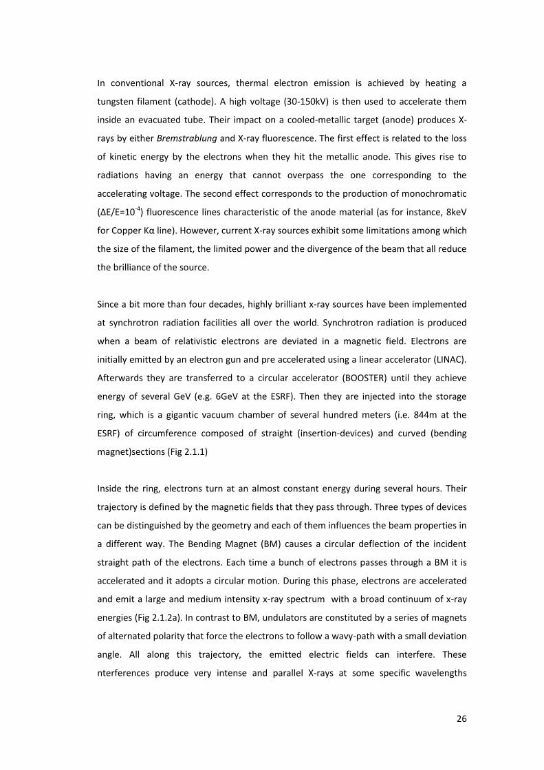
Inside the ring, electrons turn at an almost constant energy during several hours. Their

trajectory is defined by the magnetic fields that they pass through. Three types of devices

can be distinguished by the geometry and each of them influences the beam properties in

a different way. The Bending Magnet (BM) causes a circular deflection of the incident

straight path of the electrons. Each time a bunch of electrons passes through a BM it is

accelerated and it adopts a circular motion. During this phase, electrons are accelerated

and emit a large and medium intensity x-ray spectrum with a broad continuum of x-ray

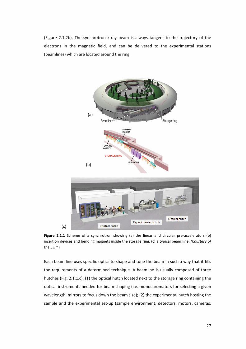
energies (Fig 2.1.2a). In contrast to BM, undulators are constituted by a series of magnets

of alternated polarity that force the electrons to follow a wavy-path with a small deviation

angle. All along this trajectory, the emitted electric fields can interfere. These

nterferences produce very intense and parallel X-rays at some specific wavelengths

27

(Figure 2.1.2b). The synchrotron x-ray beam is always tangent to the trajectory of the

electrons in the magnetic field, and can be delivered to the experimental stations

(beamlines) which are located around the ring.

Figure 2.1.1 Scheme of a synchrotron showing (a) the linear and circular pre-accelerators (b)

insertion devices and bending magnets inside the storage ring, (c) a typical beam line. (Courtesy of

the ESRF)

Each beam line uses specific optics to shape and tune the beam in such a way that it fills

the requirements of a determined technique. A beamline is usually composed of three

hutches (Fig. 2.1.1.c): (1) the optical hutch located next to the storage ring containing the

optical instruments needed for beam-shaping (i.e. monochromators for selecting a given

wavelength, mirrors to focus down the beam size); (2) the experimental hutch hosting the

sample and the experimental set-up (sample environment, detectors, motors, cameras,

(b)

(a)

(c)

28

etc) and (3) an additional room allowing researchers to control their experimental and

collect the data.

Figure 2.1.2 Synchrotron radiation produced at (bending magnet) and (b) undulators.

Nowadays light sources of this kind are becoming widespread and easily accessible.

Among the most important third generation synchrotron sources, one can cite the

Advanced Photon Source (APS) in USA, Spring-8 in Japan, Soleil in France, Petra in

Germany, Elettra in Italy and the European Synchrotron Radiation Facility (ESRF) in

Grenoble.

2.1.1. Properties

The synchrotron radiation offers several advantages for the development of

scattering/diffraction, spectroscopy, imaging and tomography techniques due to its

intrinsic properties e.g. high brilliance, tunable energy, high collimation, spatial

coherence, polarized and pulsed beams.

a) High Brilliance: The source brilliance is defined as a number of photons per

second (flux) emitted per unit area and per unit solid angle in a given

bandwidth. It is expressed in (photons/s/mm2/mrad2/0.1%bw). What makes

the synchrotron sources highly brilliant is the very weak angular divergence

that arises from the high collimation of the synchrotron beam. This is a

natural phenomenon caused by relativistic effects and by the horizontal

movement of the electrons which precludes any vertical divergence of the

beam. The narrow bandwidth of radiation and also a high flux and small

geometrical divergence results in exceptional brilliance (1x1021

photons/s/mm2/mrad2/0.1%bw for ESRF since 2011). High brilliance is of

particular importance to perform in-situ experiments and real-time

monitoring.

(b) (a)

29

b) Monocromaticity: The very high flux allows to select an homogeneous and

monochromatic beam by using single-crystal or channel cut monochromators

and by modulating the gap of undulators. Bending magnets provide a broad

continuum of X-rays energies (white beam) whereas undulators produce very

intense and parallel X- rays concentrated in narrow energy bands in the

spectrum. A single or double mirror is used for the higher harmonics

suppression.

c) Focused Beam: Due to the high collimation of the beam and the progress in X-

ray optics, micro and nano focused beams (cross sections ranging between

100µm-100nm) can be achieved and used to measure the weakly scattering

sample with high sensitivity and precision.

d) Coherent beam: The high degree of coherence of the beam allows performing

the coherence diffraction imaging techniques. Coherent properties of the X-

rays beam is characterised with the two type of coherence: transverse and

longitudinal coherences defined as [Als-Nielsen&McMorrow2010]:

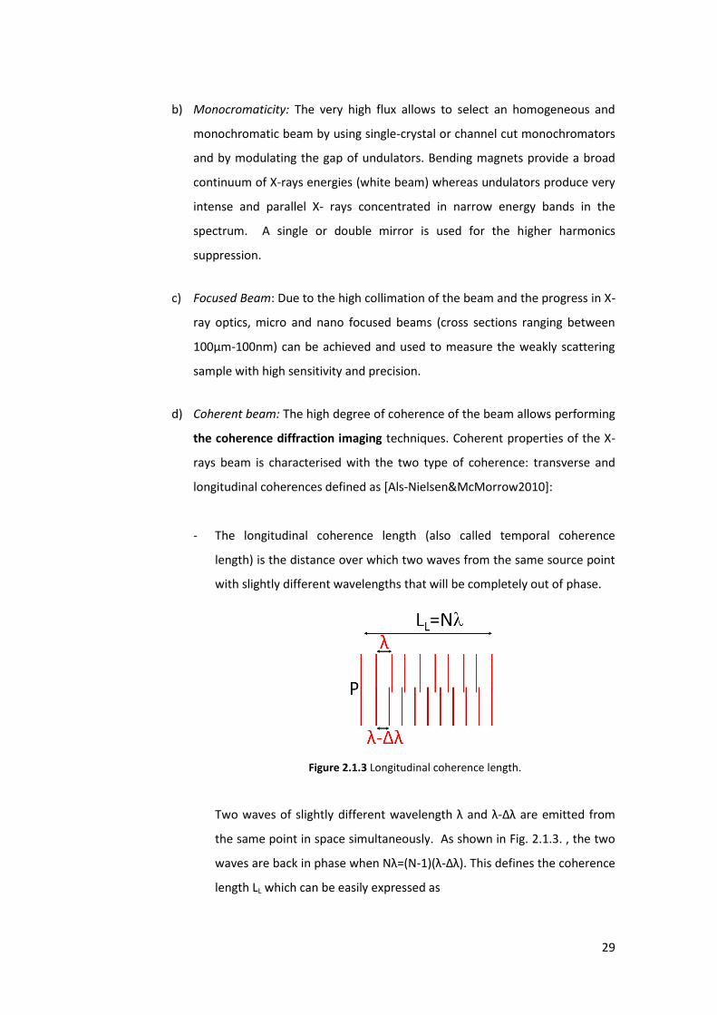
- The longitudinal coherence length (also called temporal coherence

length) is the distance over which two waves from the same source point

with slightly different wavelengths that will be completely out of phase.

Figure 2.1.3 Longitudinal coherence length.

Two waves of slightly diffe e t a ele gth a d -Δ a e e itted f o

the same point in space simultaneously. As shown in Fig. 2.1.3. , the two

a es a e a k i phase he N = N- -Δ . This defi es the ohe e e

length LL which can be easily expressed as

30

2

NLL [2.1.2]

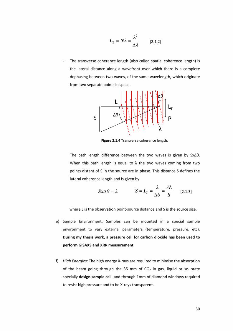
- The transverse coherence length (also called spatial coherence length) is

the lateral distance along a wavefront over which there is a complete

dephasing between two waves, of the same wavelength, which originate

from two separate points in space.

Figure 2.1.4 Transverse coherence length.

The path length difference between the two waves is given by SxΔθ.

Whe this path le gth is e ual to the two waves coming from two

points distant of S in the source are in phase. This distance S defines the

lateral coherence length and is given by

Sx S

LLS T

[2.1.3]

where L is the observation point-source distance and S is the source size.

e) Sample Environment: Samples can be mounted in a special sample

environment to vary external parameters (temperature, pressure, etc).

During my thesis work, a pressure cell for carbon dioxide has been used to

perform GISAXS and XRR measurement.

f) High Energies: The high energy X-rays are required to minimise the absorption

of the beam going through the 35 mm of CO2 in gas, liquid or sc- state

specially design sample cell and through 1mm of diamond windows required

to resist high pressure and to be X-rays transparent.

31

2.1.2. Specificity of the ID10 beam line

This section is dedicated to the description of the beamline ID10 of the European

Synchrotron Radiation Facility (ESRF) where GISAXS and XRR measurement has been

performed using the cell pressure.

The beam line is composed of two experimental hutches: one (ID10-LSIS) devoted to

structural studies on soft condensed matter surfaces and interfaces using grazing-

incidence diffraction (GID), X-ray reflectivity (XRR), grazing-incidence small-angle

scattering (GISAXS) and Grazing Incidence X-Ray Fluorescence (GIXRF) and another (ID10-

CS) fully dedicated for experiments with coherent X-rays to study slow dynamics in soft

and hard condensed matter with X-ray Photon Correlation Spectroscopy (XPCS) and to

lens-less imaging applications with Coherent Diffraction Imaging (CXDI). The X-ray source

of ID10 is composed of three independent undulator segments in series. Two segments

are stationary and host a U27 (27mm period) and a U35 (35mm period) standard ESRF

undulator, respectively. The third segment is modular (revolver-type) and either a U27 or

a U35 may be inserted rapidly and used depending on energy requirements. All

undulators are operating ex vacuum with a minimum gap of ~11 mm. This undulator

configuration allows optimizing the flux over a broad range of energies. When combining

2U27+U35 with the 1st harmonic of U27 and the 3rd harmonic of U35 tuned to 8keV the

measured peak brilliance exceeds 1020photons/s/mm2/mrad2/0.1%bw at 100mA. The

source size (FWHM) is 19µm x 945µm. ID10-LSIS is operating over a broad energy range

between 7keV and 30keV.The peak performance is achieved when the two U27 segments

are used, i.e. between 7-11keV with the first harmonic and 21-30keV with the third

harmonic. ID10-CS operates in the range 7-10keV, the range where the ID10 section

delivers the highest brilliance. The standard working energy is 8 keV where the focusing

capabilities are optimized, and the coherent flux on the sample exceeds

1x1011ph/s/100µm2 with all three undulators tuned and phased.

The optics to focus the beam at ID10 is composed of Beryllium lenses installed in a

machine named transfocator. This system allows us to focus the beam on the detector

position or at the sample position with a few micrometers size spot in a large energy

range by selecting the appropriate number of lenses.

32

Figure 2.1.5 The high resolution GISAXS setup: A – variable length evacuated flightpath; B – two

dimensional detector on the translation stage; C – optical rail. (Courtesy of the ESRF)

The ID10-LSIS has a large hutch, which allows us positioning the detector at 4m from the

sample and perform GISAXS studies on my samples of Polystyrene Island supported on

silicon. The permanent GISAXS setup comprises the optical rail (Fig.2.1.5 C), mounted on

three pillars downstream the diffractometer, the 2D MAXIPIX detector with its holder

(Fig.2.1.5 B) and the evacuated flightpath (Fig.2.1.5A).

The principle of the setup was tested for the first time during my experiments using high

energy (22keV) to minimize the absorption in air in absence of the long evacuated flight

path. The measured GISAXS image clearly shows the island-island correlation peak (Fig.

2.1.6).

Figure.2.1.6 First experimental test with the high resolution GISAXS setup. Experimental

conditions: energy - 22keV; grazing angle – 0.18 deg; sample-detector distance - 4m; detector –

Maxipix 5 x 1. Sample: polystyrene islands on a silicon wafer in CO2 atmosphere; islands height is

5nm and island-island correlation length is 100nm.

C

A B

33

Another key component that makes it possible to collect GISAXS patterns with a high

resolution is the detector. During my thesis work I had the opportunity to use the

MAXIPIX detector which has a pixel size of 55µm and working area 14x70 mm2. This

detector was developed at CERN and built at the ESRF.

2.1.3. Specificity of the ID02 beamline

Following the details about the ID02 beamline are given. This beamline was recently

upgraded and is available for the users since july. It is important to note that all the SAXS

and USAXS measurements were performed in the ID02 beamline before the upgrade

mentioned.

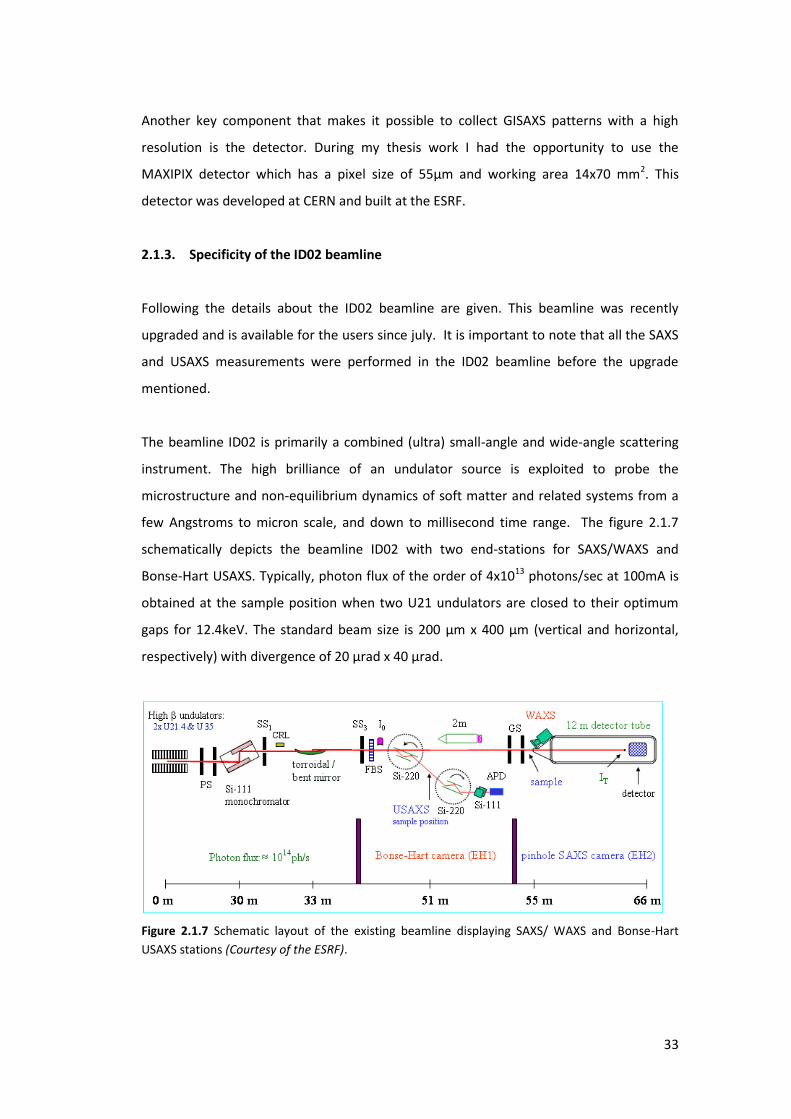
The beamline ID02 is primarily a combined (ultra) small-angle and wide-angle scattering

instrument. The high brilliance of an undulator source is exploited to probe the

microstructure and non-equilibrium dynamics of soft matter and related systems from a

few Angstroms to micron scale, and down to millisecond time range. The figure 2.1.7

schematically depicts the beamline ID02 with two end-stations for SAXS/WAXS and

Bonse-Hart USAXS. Typically, photon flux of the order of 4x1013 photons/sec at 100mA is

obtained at the sample position when two U21 undulators are closed to their optimum

gaps for 12.4keV. The standard beam size is 200 µm x 400 µm (vertical and horizontal,

respectively) with divergence of 20 µrad x 40 µrad.

Figure 2.1.7 Schematic layout of the existing beamline displaying SAXS/ WAXS and Bonse-Hart

USAXS stations (Courtesy of the ESRF).

34

The SAXS detector is mounted on a wagon inside the 12 m detector tube. The sample-to-

detector distance can be varied from 1 m to 10 m covering a wide scattering wave vector

q-range, 6x10-3 nm-1 < q < 6 nm-1, he e = / si θ/ , ith the a e le gth ~ .

nm a d θ the s atte i g a gle. The esolutio li ited the ea di e ge e ~

ad a d size ~ is a out -3nm-1. However, the smallest q reachable at 10m

detector distance is also limited by the detector point spread function and the parasitic

scattering to about 6x10-3nm-1. In normal operation, q is further curtailed to about

0.008nm-1 due to the parasitic background and limited dynamic range of the detector.

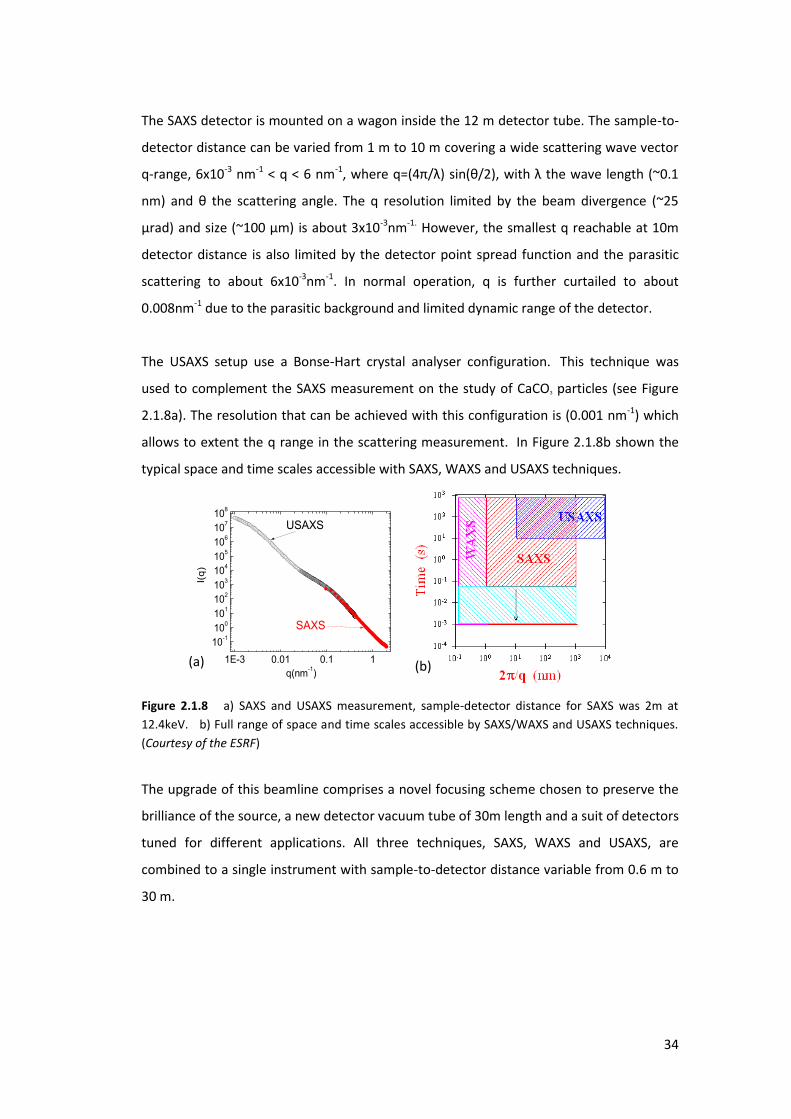
The USAXS setup use a Bonse-Hart crystal analyser configuration. This technique was

used to complement the SAXS measurement on the study of CaCO3 particles (see Figure

2.1.8a). The resolution that can be achieved with this configuration is (0.001 nm-1) which

allows to extent the q range in the scattering measurement. In Figure 2.1.8b shown the

typical space and time scales accessible with SAXS, WAXS and USAXS techniques.

1E-3 0.01 0.1 1

10-1

100

101

102

103

104

105

106

107

108

SAXS

I(q

)

q(nm-1)

USAXS

Figure 2.1.8 a) SAXS and USAXS measurement, sample-detector distance for SAXS was 2m at

12.4keV. b) Full range of space and time scales accessible by SAXS/WAXS and USAXS techniques.

(Courtesy of the ESRF)

The upgrade of this beamline comprises a novel focusing scheme chosen to preserve the

brilliance of the source, a new detector vacuum tube of 30m length and a suit of detectors

tuned for different applications. All three techniques, SAXS, WAXS and USAXS, are

combined to a single instrument with sample-to-detector distance variable from 0.6 m to

30 m.

(a) (b)

35

2.2. X-ray interaction with matter

This section deals with the presentation of the fundamental aspects of x-ray interactions

with matter which are important to explain the principles of X-ray reflectivity, GISAXS and

SAXS. A more detailed and exhaustive treatment of those techniques can be found in

several books as [Gibaud2009, Als-Nielsen&McMorrow2010].

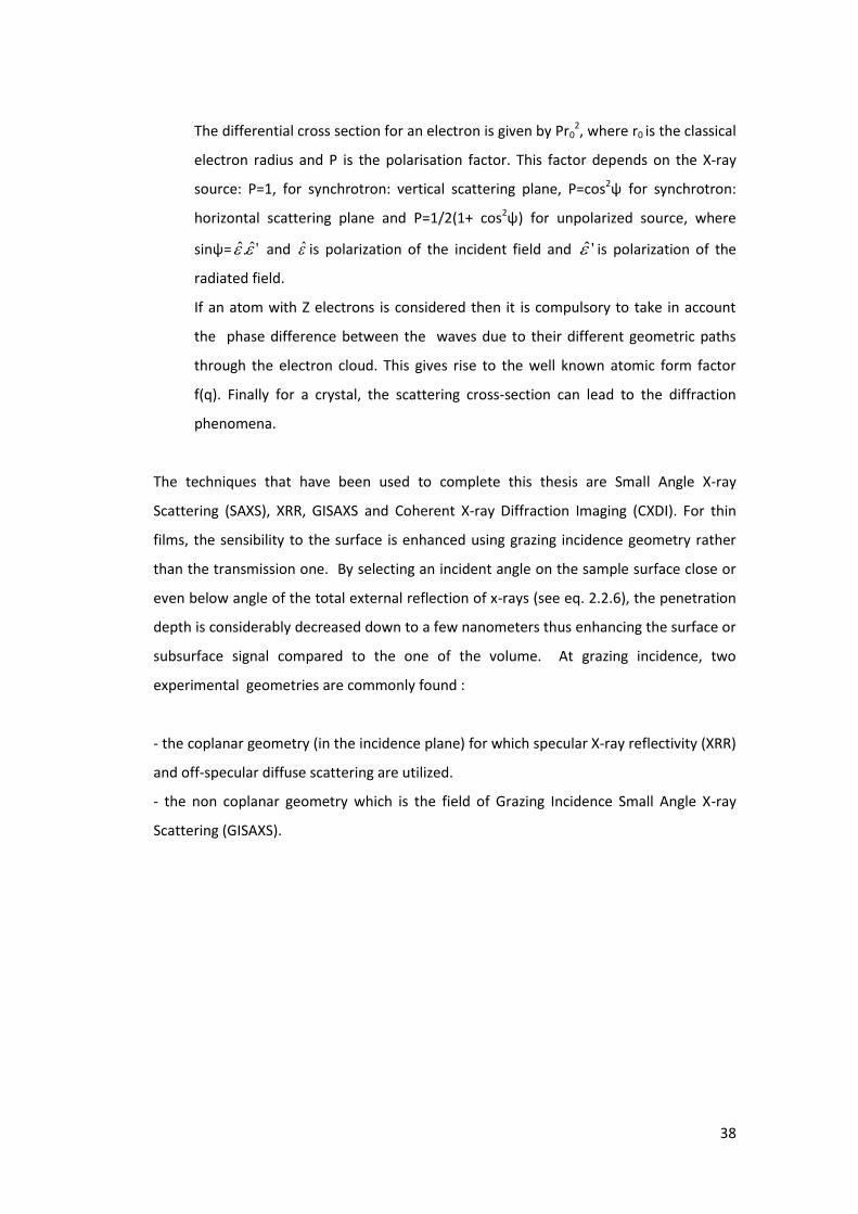
When an x-ray beam interacts with a sample, basically three processes may be observed

The incident beam may be either refracted/reflected, or scattered or absorbed. These

three processes are illustrated in the Figure 2.2.1.

Figure 2.2.1 The x-ray beam interacts with a sample in three different ways: a) absorption,

refraction, or scattering.

Absorption

In practice, the absorption is characterized by the linear absorption coefficient µ. It

is straightforward to show that the transmitted intensity I(z) at a depth z from the

surface of material at the normal incidence is given by the well known Beer-

Lambert's law

)exp()( 0 µzIzI [2.2.1]

When an x-ray photon is absorbed by an atom, its energy is transferred to some

electrons which might be either expelled from the atom leaving it ionized or

absorbed so as to increase their energy by changing their levels. The process is

known as photoelectric absorption. When the energy exceeds the threshold for

expelling an electron from a certain shell, another channel of absorption is opened

up and the cross section exhibits a discontinuous jump at the threshold energy.

These discontinuities are called absorption edges.

c) a) b)

36

Near a threshold energy, the cross section has actually more structure than just a

discontinus jump. The detailed energy dependence is called EXAFS (Extended X-ray

Absorption Fine Structure). The electron wave is scattered by the electron clouds of

neighboring atoms and interference phenomena (oscillations) occurs versus the X-

ray energy. The EXAFS spectrum is interpreted either by comparing with theoretical

models or with the spectra from known complexes.

Refraction

When the x-ray beam impinges at a surface, it slightly changes its direction by

refraction (Fig. 2.2.1b). This phenomenon, very well known for visible light, is for

instance responsible for the deviation of light when it passed through a prism. X-

ray beams can also be refracted. However the refractive index of a material for X-

rays does not differ very much from unity so that refraction is barely visible. The

refractive index can be expressed as [Born&Wolf1980]

in 1 [2.2.2]

he e a d β a ou t fo the s atte i g a d a so ptio of the ate ial,

respectively. The values of a d β hi h a e positi e depe d o the ele t o

de sit , e, and linear absorption coefficient, µ, of the material through the

following relations

ee

k m

kke r

V

fZr

22

2

'

2

[2.2.3]

4

''

22

k m

ke

V

fr [2.2.4]

where re = 2.813 .10-5 Å is the classical radius of the electron, Vm is the volume of

the unit cell, Zk is the u e of ele t o s of the ato k i the u it ell, f a d f" a e

the real and imaginary parts of the atomic scattering factor for the specific energy

of the i ide t adiatio . Note that these relations stand for crystalline materials

only but can be also expressed for liquids or amorphous materials if their density is

known.

37

In view of the fact that δ is positive, the refractive index of a material is always

smaller than unity. Passing from vacuum (n = 1) to the reflecting material (n < 1), it

is possi le to totall efle t the ea if the g azi g a gle α hi h is the a gle

between the surface of the sample and the incident beam) is small enough (below

few milli-radians). This is known as the total external reflection of X-rays. For this

to o u , the i ide t a gle ust e s alle tha the iti al a gle αc defined by the

“ ell s la as:

inc 1cos [2.2.5]

“i e >> >> 0 the expression for critical angle can be approximated as [Als-

Nielsen&McMorrow2010]

ee

c

r

22 2 [2.2.6]

Scattering

The scattering process is illustrated in Fig. 2.2.1c in which an X-ray beam of intensity

I0 photons per second is incident on a sample, and where the sample is large

enough that it intercepts the entire beam. Our objective is to calculate the number

of X-ray photons, ISC, scattered per second into a detector that subtends a solid

a gle ΔΩ. If the e a e N pa ti les i the sa ple pe u it a ea see alo g the ea

direction, then ISC will be proportional to N and to I0. It will of course also be

p opo tio al to ΔΩ. Most i portantly it will depend on how efficiently the particles

in the sample scatter the radiation, this is given by the differential cross-section,

dσ/dΩ , so that e a ite

d

dNII sc

0 [2.2.7]

Thus the differential cross –section per scattering particle will be defined by:

NId

d

0

into secondper scattered photonsray -X of No. [2.2.8]

38

The differential cross section for an electron is given by Pr02, where r0 is the classical

electron radius and P is the polarisation factor. This factor depends on the X-ray

source: P=1, for synchrotron: vertical scattering plane, P=cos2ψ for synchrotron:

horizontal scattering plane and P=1/2(1+ cos2ψ fo unpolarized source, where

si ψ= 'ˆ.ˆ and ̂ is polarization of the incident field and '̂ is polarization of the

radiated field.

If an atom with Z electrons is considered then it is compulsory to take in account

the phase difference between the waves due to their different geometric paths

through the electron cloud. This gives rise to the well known atomic form factor

f(q). Finally for a crystal, the scattering cross-section can lead to the diffraction

phenomena.

The techniques that have been used to complete this thesis are Small Angle X-ray

Scattering (SAXS), XRR, GISAXS and Coherent X-ray Diffraction Imaging (CXDI). For thin

films, the sensibility to the surface is enhanced using grazing incidence geometry rather

than the transmission one. By selecting an incident angle on the sample surface close or

even below angle of the total external reflection of x-rays (see eq. 2.2.6), the penetration

depth is considerably decreased down to a few nanometers thus enhancing the surface or

subsurface signal compared to the one of the volume. At grazing incidence, two

experimental geometries are commonly found :

- the coplanar geometry (in the incidence plane) for which specular X-ray reflectivity (XRR)

and off-specular diffuse scattering are utilized.

- the non coplanar geometry which is the field of Grazing Incidence Small Angle X-ray

Scattering (GISAXS).

39

2.3. X-ray reflectivity (XRR)

The XRR measurement technique described in this section is used to analyse the X-ray

reflection intensity as a function of the grazing angle to determine parameters of a thin-

film including the thickness, density, and roughness. This section provides a quick

overview of the principles of X-ray reflectivity and the analysis methods [Gibaud2009].

2.3.1. General principles

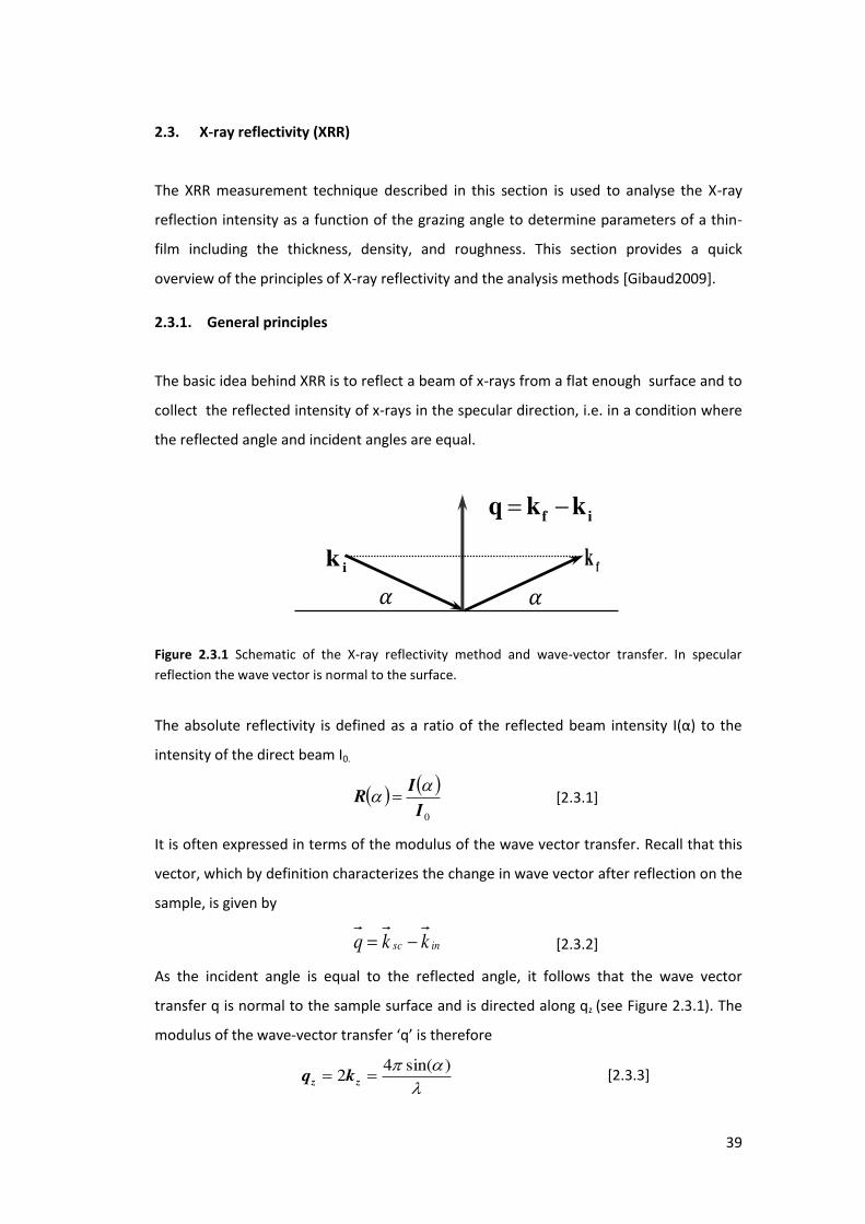
The basic idea behind XRR is to reflect a beam of x-rays from a flat enough surface and to

collect the reflected intensity of x-rays in the specular direction, i.e. in a condition where

the reflected angle and incident angles are equal.

Figure 2.3.1 Schematic of the X-ray reflectivity method and wave-vector transfer. In specular

reflection the wave vector is normal to the surface.

The a solute efle ti it is defi ed as a atio of the efle ted ea i te sit I α to the

intensity of the direct beam I0.

0I

IR

[2.3.1]

It is often expressed in terms of the modulus of the wave vector transfer. Recall that this

vector, which by definition characterizes the change in wave vector after reflection on the

sample, is given by

insc kkq [2.3.2]

As the incident angle is equal to the reflected angle, it follows that the wave vector

transfer q is normal to the sample surface and is directed along qz (see Figure 2.3.1). The

modulus of the wave- e to t a sfe is therefore

)sin(4

2 zz kq [2.3.3]

ik

f iq k k

fk

40

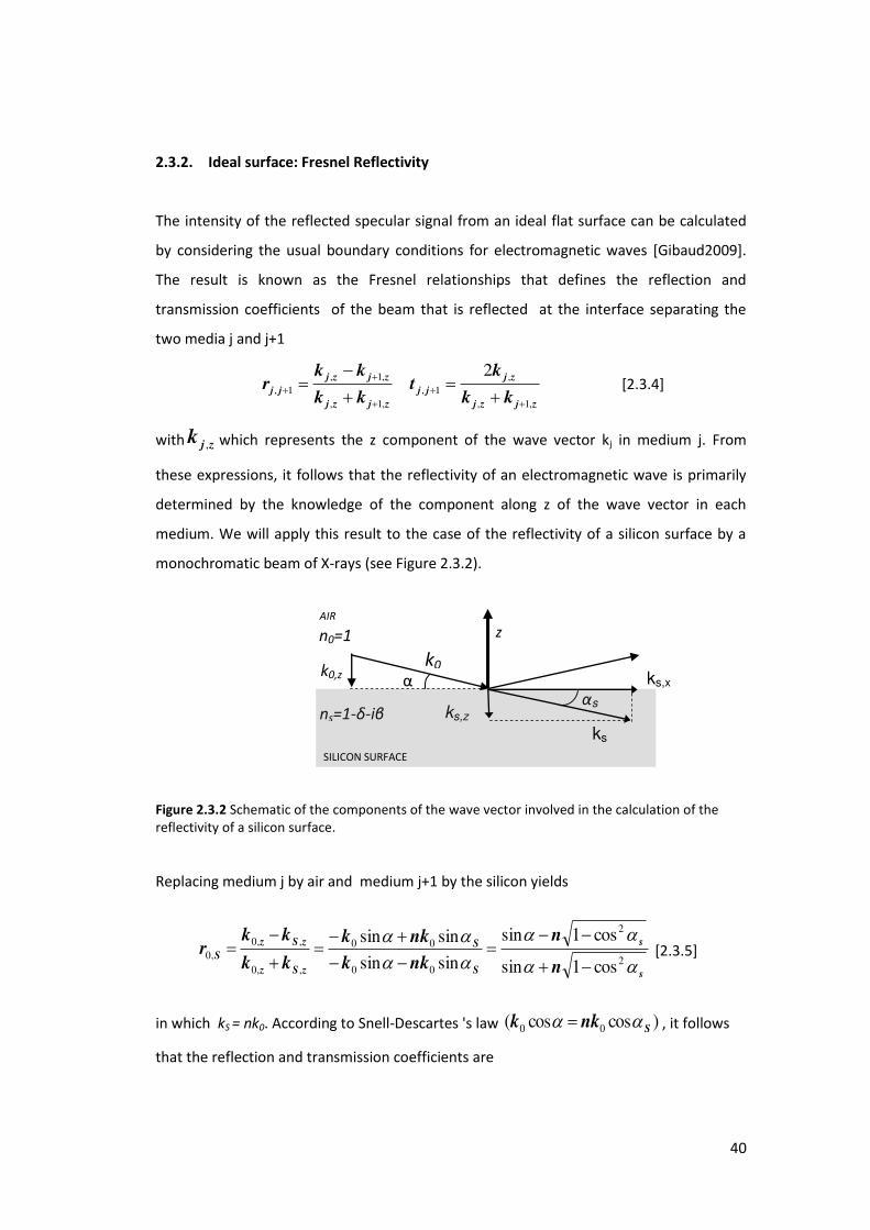
2.3.2. Ideal surface: Fresnel Reflectivity

The intensity of the reflected specular signal from an ideal flat surface can be calculated

by considering the usual boundary conditions for electromagnetic waves [Gibaud2009].

The result is known as the Fresnel relationships that defines the reflection and

transmission coefficients of the beam that is reflected at the interface separating the

two media j and j+1

zjzj

zj

jj

zjzj

zjzj

jjkk

kt

kk

kkr

,1,

,1,

,1,

,1,1,

2

[2.3.4]

with zjk , which represents the z component of the wave vector kj in medium j. From

these expressions, it follows that the reflectivity of an electromagnetic wave is primarily

determined by the knowledge of the component along z of the wave vector in each

medium. We will apply this result to the case of the reflectivity of a silicon surface by a

monochromatic beam of X-rays (see Figure 2.3.2).

Figure 2.3.2 Schematic of the components of the wave vector involved in the calculation of the reflectivity of a silicon surface.

Replacing medium j by air and medium j+1 by the silicon yields

s

s

S

S

zSz

zSz

S

n

n

nkk

nkk

kk

kkr

2

2

00

00

,,0

,,0,0

cos1sin

cos1sin

sinsin

sinsin

[2.3.5]

in which kS = nk0. According to Snell-Descartes 's law )coscos( 00 Snkk , it follows

that the reflection and transmission coefficients are

AIR

z n0=1

k0

α k0,z ks,x

αs ns=1-δ-iβ ks,z

ks

SILICON SURFACE

41

22,022

22

,0cossin

sin2

cossin

cossin

nt

n

nr SS

[2.3.6]

At small angle of incidence and with n close to 1, the reflectivity and transmitted

intensity are given by

2

2

2

2

2

22

2

22

22

iT

i

iR

[2.3.7]

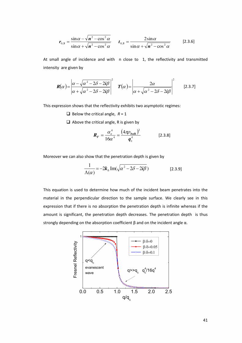
This expression shows that the reflectivity exhibits two asymptotic regimes:

Below the critical angle, R = 1

Above the critical angle, R is given by

4

2

4

4 416 z

bulkcF

qR

[2.3.8]

Moreover we can also show that the penetration depth is given by

)22Im(2)(

1 20

ik

[2.3.9]

This equation is used to determine how much of the incident beam penetrates into the

material in the perpendicular direction to the sample surface. We clearly see in this

expression that if there is no absorption the penetration depth is infinite whereas if the

amount is significant, the penetration depth decreases. The penetration depth is thus

strongly depending on the absorption coefficient β a d o the i ide t a gle α.

0.0 0.5 1.0 1.5 2.0 2.5

1

q<qc

evanescent

wave

Fre

sn

el R

efle

ctivity

q/qc

q>>qc q

4

c/16q

4

42

0.0 0.5 1.0 1.5 2.0 2.50

1

2

3

4

Tra

nsm

issio

n

q/qc

maximum

value

0.0 0.5 1.0 1.5 2.0 2.5

101

102

103

bulk

Pe

ne

tra

tio

n d

ep

th (

)

q/qc

surface

Figure 2.3.3 The efle ti it ‘, the t a s issio T a d the pe et atio depth Λ e sus / c. In each

ase, a fa il of u es is gi e o espo di g to diffe e t alues of to the atio β / . Whe << there is total reflection and the reflected wave propagates along the surface with a minimal

penetration depth of 1/qc. Due to the small penetration depth, this wave is called an evanescent

wave. When q>>1 the reflectivity falls off as R(q)=1/(q)4 and there is almost complete

transmission.

2.3.3. Reflectivity from a layered material

2.3.3.1. Dynamical Theory (Matrix Formalism)

When the wave propagates in heterogeneous medium presenting regions of different

electron densities, it is not possible to directly use the Fresnel relationship. The

calculation is performed by applying the boundary conditions of the electric and magnetic

fields at each interface [Gibaud1999, Parrat1954, and Born1980]. The fact that multiple

reflections are taken into account in the calculation leads to the dynamical theory of

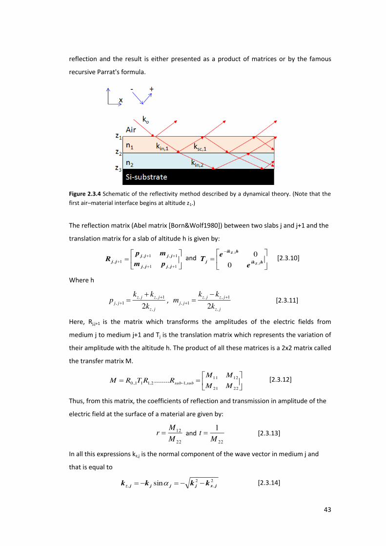
43

reflection and the result is either presented as a product of matrices or by the famous

recursive Parrat's formula.

Figure 2.3.4 Schematic of the reflectivity method described by a dynamical theory. (Note that the

first air–material interface begins at altitude z1.)

The reflection matrix (Abel matrix [Born&Wolf1980]) between two slabs j and j+1 and the

translation matrix for a slab of altitude h is given by:

1,1,

1,1,1,

jjjj

jjjj

jj pm

mpR and

hik

hik

jZ

Z

e

eT

1,

1,

0

0 [2.3.10]

Where h

. , 1

, 1,2

z j z j

j j

z j

k kp

k

,

. , 1, 1

,2z j z j

j j

z j

k km

k

[2.3.11]

Here, Rj,j+1 is the matrix which transforms the amplitudes of the electric fields from

medium j to medium j+1 and Tj is the translation matrix which represents the variation of

their amplitude with the altitude h. The product of all these matrices is a 2x2 matrix called

the transfer matrix M.

2221

1211,12,111.,0 ........

MM

MMRRTRM subsub

[2.3.12]

Thus, from this matrix, the coefficients of reflection and transmission in amplitude of the

electric field at the surface of a material are given by:

22

12

M

Mr and

22

1M

t [2.3.13]

In all this expressions kz,j is the normal component of the wave vector in medium j and

that is equal to

2,

2, sin jxjjjjz kkkk [2.3.14]

44

kx,j is o se ed a d it is e ual to k osα. As the esult of this, the z o po e t of k0 in

medium j is

220

220, cosknkk jjz [2.3.15]

Where k0 is the wave vector in air. In the limit of small angle and substituting the

expression of the refractive index for x-rays, this becomes

220

20, 22 cjjjz kikk and 22

, czjz qqq [2.3.16]

A similar expressions can be obtained for kz,j+1 so that the coefficients pj,j+1 and mj,j+1 are

e ti el dete i ate the i ide t a gle a d the alue of a d β i each layer.

For example for a single layer on a substrate, the transfer matrix is given by

2,12,1

2,12,1

1,01,0

1,01,02,111,0

1,

1,

0

0pm

mp

e

e

pm

mpRTR

hik

hik

Z

Z

[2.3.17]

Then considering that the reflection coefficients is r=M11/M22 and introducing the

reflection coefficients 1,1,1, / jjjjjj pmr at the interface j,j+1 we get:

hik

hik

LAYER

z

z

err

errr

1,

1,

22,11,0

22,11,0

1

[2.3.18]

It is worth noting that the denominator of this expression differs from unity by a term

which corresponds to multiple reflections in the material as evidenced by the product of

the two reflection coefficients 2,11,0 rr .

2.3.3.2. Kinematical Theory

The full dynamical theory described above is exact but does not clearly show the physics

of scattering because numerical calculations are necessary. Sometimes, one can be more

interested in an approximated analytical expression. That is why the use of the

kinematical theory which simplifies the expression of the reflected intensity taking in

accounts the three Born approximations [Born1980, Hamley1994, Gibaud2009].

45

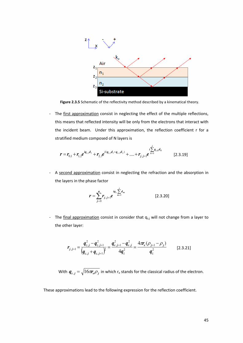
Figure 2.3.5 Schematic of the reflectivity method described by a kinematical theory.

- The first approximation consist in neglecting the effect of the multiple reflections,

this means that reflected intensity will be only from the electrons that interact with

the incident beam. Under this approximation, the reflection coefficient r for a

stratified medium composed of N layers is

j

k

kkz

zzz

dqi

jj

dqdqidiqerererrr 0

,22,11,11,

1,)(

3,22,11,0 .... [2.3.19]

- A second approximation consist in neglecting the refraction and the absorption in

the layers in the phase factor

n

j

diq

jj

j

m

mz

err0

1,0 [2.3.20]

- The final approximation consist in consider that qz,j will not change from a layer to

the other layer:

2

1

2

2,

21,

21,,

21,

2,

1,

)(4

4 z

jje

z

jcjc

jzjz

jzjz

jjq

r

q

qq

qq

qqr

[2.3.21]

With jejc rq 16, in which re stands for the classical radius of the electron.

These approximations lead to the following expression for the reflection coefficient.

46

n

j

diq

z

jj

e

j

m

mz

eq

rr0

2

1 0)(

4

[2.3.22]

If the origin of the z axis is chosen to be at the upper surface (medium 0 at the depth

Z1=0), then the sum over dm in the phase factor can be replaced by the depth Zj+1 of the

interface j,j+1 and the equation becomes

n

j

Ziq

z

jj

e

jzeq

rr0

2

1 1)(

4

[2.3.23]

Finally, the kinematic theory make it possible to write the reflectivity of the materials

composed by n layers for angles far from the total reflection as:

2

02

1 1)(

4)(

n

j

Ziq

z

jj

ez

jzeq

rqR

[2.3.24]

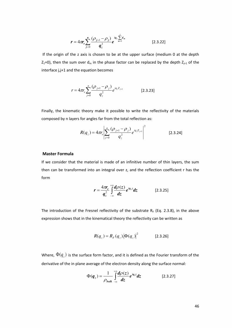
Master Formula

If we consider that the material is made of an infinitive number of thin layers, the sum

then can be transformed into an integral over z, and the reflection coefficient r has the

form

dzedz

zd

q

rr

ziq

z

e z)(4

2

[2.3.25]

The introduction of the Fresnel reflectivity of the substrate RF (Eq. 2.3.8), in the above

expression shows that in the kinematical theory the reflectivity can be written as

2)().()( zzFz qqRqR [2.3.26]

Where, )( zq is the surface form factor, and it is defined as the Fourier transform of the

derivative of the in plane average of the electron density along the surface normal:

dzedz

zdq

ziq

bulk

zz

)(1)(

[2.3.27]

47

The above expression of R(qz) is not rigorous but can be easily handled in analytical

calculations ( bulk is the electron density of the substrate bulk).

2.3.4. Analysis of the curves

As seen above, the quantitative analysis of X-ray reflectivity curves may be obtained

through curve fitting calculations based on the matrix formalism. However, this procedure

requires a prior knowledge of the system; this information can be obtained by performing

a preliminary qualitative study of curves. In this section is described in detail the

information that can be obtained on a layered material layer by using a simple qualitative

analysis of the experimental curves.

We illustrate as an example the cases of two systems that we have studied in this thesis:

- the determination of the electron density obtained from the XRR measurements of a

film of polystyrene deposited on a silicon substrate.

- the XRR characteristics of a thin film of mesoporous silica deposited on a silicon

substrate.

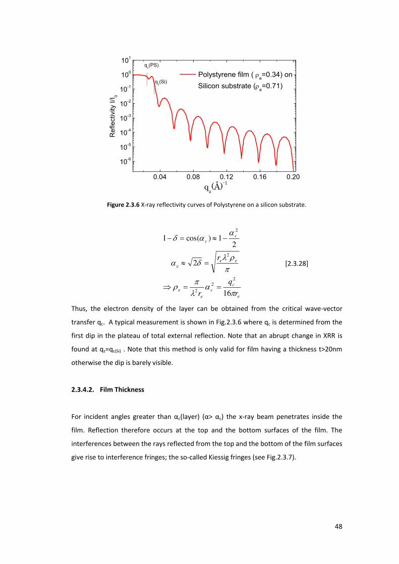
2.3.4.1. Electron density of a PS film

Fo ualitati e dis ussio , it is ade uate to o side a a so ptio lose to β= ut it

should e oted that β a ot e ig o ed i the si ulatio of X‘‘. Fo i ide t a gles

elo the iti al a gle α<αc) of PS, total reflection occurs. By appl i g “ ell s la a d

small angle approximations, the critical angle can be expressed as:

48

0.04 0.08 0.12 0.16 0.20

10-6

10-5

10-4

10-3

10-2

10-1

100

101

qc(Si)

Polystyrene film ( e=0.34) on

Silicon substrate (e=0.71)

Re

fle

ctivity I

/I0

qz(Å)

-1

qc(PS)

Figure 2.3.6 X-ray reflectivity curves of Polystyrene on a silicon substrate.

e

c

c

e

e

ee

c

c

r

q

r

r

16

2

21 )cos(1

22

2

2

c

2

[2.3.28]

Thus, the electron density of the layer can be obtained from the critical wave-vector

transfer qc. A typical measurement is shown in Fig.2.3.6 where qc is determined from the

first dip in the plateau of total external reflection. Note that an abrupt change in XRR is

found at qz=qc(Si) . Note that this method is only valid for film having a thickness t>20nm

otherwise the dip is barely visible.

2.3.4.2. Film Thickness

Fo i ide t a gles g eate tha αc la e α> αc) the x-ray beam penetrates inside the

film. Reflection therefore occurs at the top and the bottom surfaces of the film. The

interferences between the rays reflected from the top and the bottom of the film surfaces

give rise to interference fringes; the so-called Kiessig fringes (see Fig.2.3.7).

49

0.0 0.1 0.2 0.3

10-6

10-5

10-4

10-3

10-2

10-1

100

Film h= 160nm

Re

fle

ctivity I

/I0

qz(Å)-1

qz=q

b

z-q

a

z

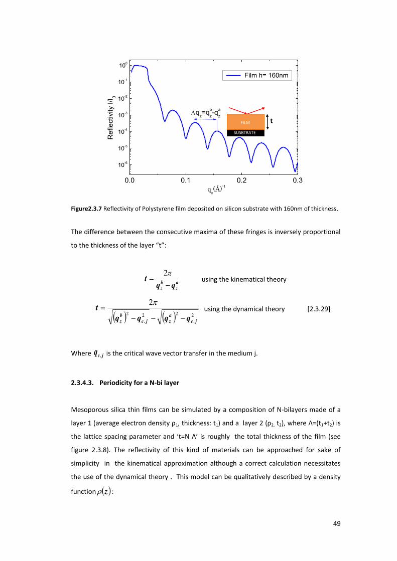
Figure2.3.7 Reflectivity of Polystyrene film deposited on silicon substrate with 160nm of thickness.

The difference between the consecutive maxima of these fringes is inversely proportional

to the thi k ess of the la e t :

a

z

b

z qqt

2 using the kinematical theory

2,

22,

2

2

jc

a

zjc

b

z qqqq

t

using the dynamical theory [2.3.29]

Where jcq , is the critical wave vector transfer in the medium j.

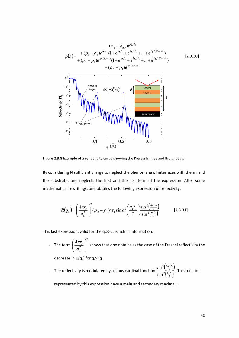
2.3.4.3. Periodicity for a N-bi layer

Mesoporous silica thin films can be simulated by a composition of N-bilayers made of a

la e a e age ele t o de sit 1, thickness: t1) and a la e 2, t2 , he e Λ= t1+t2) is

the latti e spa i g pa a ete a d t=N Λ is oughl the total thi k ess of the film (see

figure 2.3.8). The reflectivity of this kind of materials can be approached for sake of

simplicity in the kinematical approximation although a correct calculation necessitates

the use of the dynamical theory . This model can be qualitatively described by a density

function z :

t PS film

ggggt SUSBTRATE

FILM

50

)(

1

)1('2)(12

)1('221

2

2

12

2

0

)(

)...1()(

)...1()(

)(

tNiq

S

Niqiqiqttiq

Niqiqiqtiq

Ziq

air

z

zzzz

zzzz

z

e

eeee

eeee

e

z

[2.3.30]

0.1 0.2 0.3

10-6

10-5

10-4

10-3

10-2

10-1

100

Re

fle

ctivity I

/I0

qz(Å)

-1

qz=q

B

z-q

A

z

Bragg peak

Kiessig

fringes

Figure 2.3.8 Example of a reflectivity curve showing the Kiessig fringes and Bragg peak.

By considering N sufficiently large to neglect the phenomena of interfaces with the air and

the substrate, one neglects the first and the last term of the expression. After some

mathematical rewritings, one obtains the following expression of reflectivity:

2

22

212

12

12

2

2 sin

sin

2sin)(

4

z

z

q

Nq

z

z

ez

tqct

q

rqR

[2.3.31]

This last expression, valid for the qz>>qc is rich in information:

- The term

2

2

4

z

e

q

r shows that one obtains as the case of the Fresnel reflectivity the

decrease in 1/qz4 for qz>>qc.

- The reflectivity is modulated by a sinus cardinal function 2

22

2

sin

sin

z

z

q

Nq

. This function

represented by this expression have a main and secondary maxima :

substrate

Λ

t

SUSBTRATE

Layer2

Layer1

51

The main maximum, called Bragg peak has a period:

A

z

B

z qq

2 using the kinematical theory

2,

22,

2

2

jc

A

zjc

B

z qqqq

using the dynamical theory [2.3.32]

The secondary maxima are less intense and are related to the Kiessig fringes of

period

a

z

b

z qqNt

2 using the kinematical theory

2

,

22,

2

2

jc

a

zjc

b

z qqqq

t

using the dynamical theory [2.3.33]

Where jcq , is the critical wave vector transfer in the medium j.

2.4. Small angle X-ray Scattering (SAXS)

SAXS contrary to XRR is a technique used in transmission through the volume of the

sample. The objective of this technique is to measure the scattered signal by large objects

(from a few angstroms to micron scale) contained in the sample which requires working

at small angle.

A schematic description of scattering principle is shown in Fig. 2.4.1. X-rays from the

source are collimated into a fine beam, often by slits, and strike the samples. A small

fraction of this beam is scattered in other directions, e. g. an angle 2θ with the direction of

the incoming beam. D is a detector, used to record the scattering intensity (the square of

the scattering amplitude) and its dependence on the scattering angle. During an

experiment of SAXS, it is recommended, in order to obtain absolute intensity, to

easu e the i te sit of the di e t ea as ell as the t a s issio T and the

thickness of the sa ple e . From the practical point of view, one has

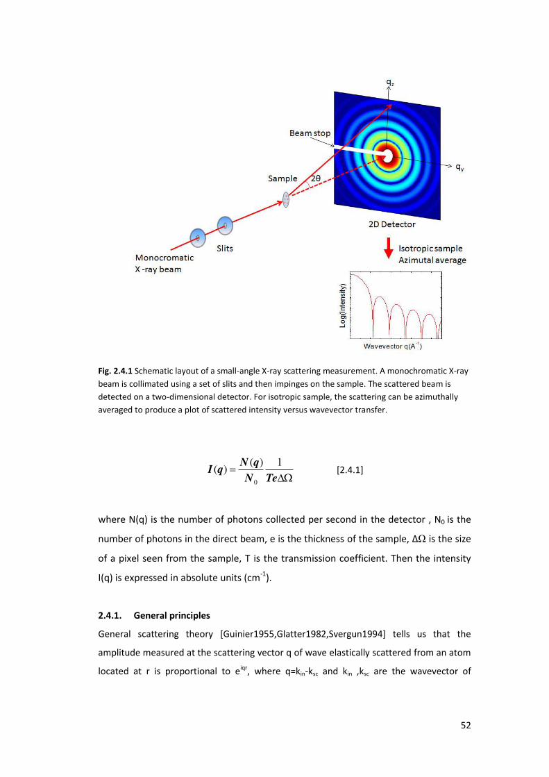
52

Fig. 2.4.1 Schematic layout of a small-angle X-ray scattering measurement. A monochromatic X-ray

beam is collimated using a set of slits and then impinges on the sample. The scattered beam is

detected on a two-dimensional detector. For isotropic sample, the scattering can be azimuthally

averaged to produce a plot of scattered intensity versus wavevector transfer.

TeN

qNqI

1)()(

0

[2.4.1]

where N(q) is the number of photons collected per second in the detector , N0 is the

number of photons in the direct beam, e is the thickness of the sample, ΔΩ is the size

of a pixel seen from the sample, T is the transmission coefficient. Then the intensity

I(q) is expressed in absolute units (cm-1).

2.4.1. General principles

General scattering theory [Guinier1955,Glatter1982,Svergun1994] tells us that the

amplitude measured at the scattering vector q of wave elastically scattered from an atom

located at r is proportional to eiqr, where q=kin-ksc and kin ,ksc are the wavevector of

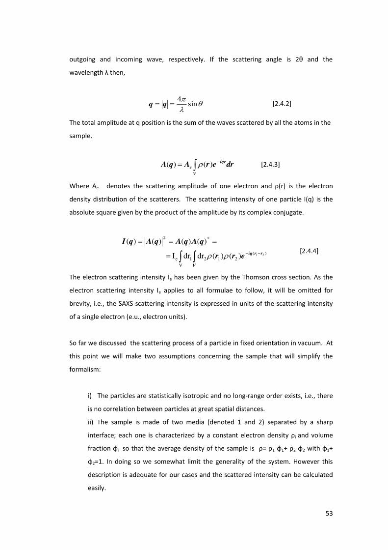
53

outgoi g a d i o i g a e, espe ti el . If the s atte i g a gle is θ a d the

wavele gth the ,

sin4

qq [2.4.2]

The total amplitude at q position is the sum of the waves scattered by all the atoms in the

sample.

drerAqAV

iqr

e )()( [2.4.3]

Where Ae denotes the scattering amplitude of o e ele t o a d is the electron

density distribution of the scatterers. The scattering intensity of one particle I(q) is the

absolute square given by the product of the amplitude by its complex conjugate.

)()(drdrI

)()()()()(

212

V

1e

*2

21

V

rriqerr

qAqAqAqI

[2.4.4]

The electron scattering intensity Ie has been given by the Thomson cross section. As the

electron scattering intensity Ie applies to all formulae to follow, it will be omitted for

brevity, i.e., the SAXS scattering intensity is expressed in units of the scattering intensity

of a single electron (e.u., electron units).

So far we discussed the scattering process of a particle in fixed orientation in vacuum. At

this point we will make two assumptions concerning the sample that will simplify the

formalism:

i) The particles are statistically isotropic and no long-range order exists, i.e., there

is no correlation between particles at great spatial distances.

ii) The sample is made of two media (denoted 1 and 2) separated by a sharp

interface; each one is characterized by a constant electron densit i and volume

f a tio φi so that the a e age de sit of the sa ple is = 1 φ1+ 2 φ2 ith φ1+

φ2=1. In doing so we somewhat limit the generality of the system. However this

description is adequate for our cases and the scattered intensity can be calculated

easily.

54

Figure 2.4.2 Two-dimensional representation of a sample containing two media

separated by sharp interface.

In this case the average over all orientations leads to the fundamental formula of

Debye,

)sin(

qr

qre iqr

[2.4.5]

Thus, equation [2.4.4] reduces to the form

qr

sin(qr)(r)4)( 2

0

drrqI

[2.4.6]

Equation [2.4.6] is the most general formula for the scattering pattern of any

systems, which obey the above two est i tio s. is the so-called correlation

function [Debye&Bueche1949], or characteristic function . It can be obtained by the

inverse Fourier transform with

qr

sin(qr)(q)

2

1)( 2

02

dqqIr

[2.4.7]

The invariant

To get a more physical insight in the meaning of the correlation function let us to imagine

that we draw, at random a line of length r on the two dimensional image of our sample

(Fig. 2.4.2) and we count how many times both ends are in medium 1, or in medium 2, or

one end in each medium and we define the associated probabilities as P11, P22 and P12

respectively. If the two media are distributed in a completely random way, then

,2111 P ,2

222 P 212112 PP [2.4.8]

If there is a correlation in the distribution of the two media, there will be some deviation

to those probabilities that can be described by a function )(0 r such that:

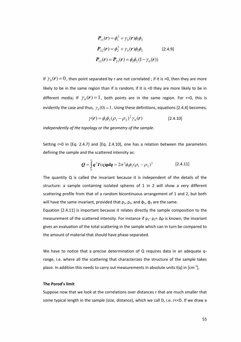
55

2102

111 )()( rrP

2102222 )()( rrP [2.4.9]

))(1()()( 0212112 rrPrP

If 0)(0 r , then point separated by r are not correlated ; if it is >0, then they are more

likely to be in the same region than if is random; if it is <0 they are more likely to be in

different media; If 1)(0 r , both points are in the same region. For r=0, this is

evidently the case and thus, 1)0(0 . Using these definitions, equations [2.4.4] becomes,

)()()( 02

2121 rr [2.4.10]

independently of the topology or the geometry of the sample.

Setting r=0 in [Eq. 2.4.7] and [Eq. 2.4.10], one has a relation between the parameters

defining the sample and the scattered intensity as:

22121

2

0

2 )(2(q)

qdqIqQ [2.4.11]

The quantity Q is called the invariant because it is independent of the details of the

structure: a sample containing isolated spheres of 1 in 2 will show a very different

scattering profile from that of a random bicontinuous arrangement of 1 and 2, but both

ill ha e the sa e i a ia t, p o ided that 1, 2, a d φ1, φ2 are the same.

Equation [2.4.11] is important because it relates directly the sample composition to the

easu e e t of the s atte ed i te sit . Fo i sta e if 1- 2= Δ is k o , the i a ia t

gives an evaluation of the total scattering in the sample which can in turn be compared to

the amount of material that should have phase-separated.

We have to notice that a precise determination of Q requires data in an adequate q-

range, i.e. where all the scattering that characterizes the structure of the sample takes

place. In addition this needs to carry out measurements in absolute units I(q) in [cm-1].

The Porod s li it

Suppose now that we look at the correlations over distances r that are much smaller that

some typical length in the sample (size, distance), which we call D, i.e. r<<D. If we draw a

56

line as we did previously, most of these will have both ends in the same phase an only

those line crossing an interface will be weighted by a non-ze o Δ a d ill pa ti ipate to

the s atte ed i te sit at la ge s >>D-1). Hence data in that region will only contain

information about the characteristics of the interface.

An exact calculation shows that the surface area per u it olu e Ʃ=“/V is elated to the

scattered intensity by

)(

2

1 42 lim qIqV q

[2.4.12]

Or, using the invariant to eliminate scale constants,

)(421 lim qIqQ q

[2.4.13]

2.4.2. Structural parameters

Valua le i fo atio a e gai ed f o dete i atio of the i a ia t a d Po od s li it

but these are independent of the geometry of the two media in the sample and hence,

are of no use to describe the structure. However, some structural parameters can be

extracted from the intensity profile.

2.4.2.1. The form factor of isolated particle

The simplest case to analyse is a dilute solution of molecules, or more generally particles,

allowing inter-particle correlations to be neglected, and where it is assumed that the

particles are identical. If the scattering length density of each particle is uniform and

ep ese ted 1, and that of the solvent is 2, then the intensity scattered normalized by

a single particle is

2

3221 )()(

Vp

iqr rdeqI [2.4.14]

Where Vp is the volume of the particle. By introducing the single particle form factor,

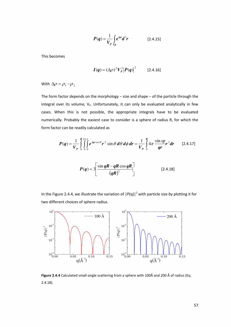
57

Vp

iqr

P

rdeV

qP 31)( [2.4.15]

This becomes

222 )()()( qPVqI P [2.4.16]

With 21

The form factor depends o the o pholog − size a d shape − of the pa ti le th ough the

integral over its volume, VP. Unfortunately, it can only be evaluated analytically in few

cases. When this is not possible, the appropriate integrals have to be evaluated

numerically. Probably the easiest case to consider is a sphere of radius R, for which the

form factor can be readily calculated as

drrqrV

drddreV

qP

R

P

R

iqr

P

2

00

2

0 0

2cos qr sin4

1 sin

1)(

[2.4.17]

3

cossin3)(

qR

qRqRqRqP [2.4.18]

In the Figure 2.4.4, we illustrate the variation of |P(q)|2 with particle size by plotting it for

two different choices of sphere radius.

0.00 0.05 0.10 0.1510

-6

10-4

10-2

100

0.00 0.05 0.10 0.1510

-6

10-4

10-2

100

100 Å

|P

(q)|

2

q(Å-1)

200 Å

|P

(q)|

2

q(Å-1)

Figure 2.4.4 Calculated small-angle scattering from a sphere with 100Å and 200 Å of radius (Eq.

2.4.18).

58

2.4.2.2. Guinier analysis

At low q region, i.e., for qr << 1 the Debye factor sin(qr)/(qr) ≅ 1 - / ! + …, e . [ .4.6]

reduces to [Guinier1939]

3

Rq-1(0)I ....

6

qr-1(r)4)(

2g

2

02

0

2

drrqI [2.4.19]

Where Rg is the radius of gyration given by

dss

dsssRg

)(

)( 2

2

[2.4.20]

With defi i g s as the e to take f o the e te of g a it of .

For homogeneous particles, the radius of gyration is only related to the geometrical

parameters of simple triaxal bodies [Mittelbach1964], e.g., RRg 5/3 for spheres with

radius R.

Because e-x ≅ 1-x, for qr << 1 eq. [2.4.19] can be also expressed as

3exp)0()(

22

0gRq

IqI [2.4.21]

This is so-called Gui ie s la , hi h is a ost useful elatio i “AX“ a al sis si e it

allows to obtaining Rg and I0(0) from the scattering data in the region of smallest angles

without any prior assumption on the shape and internal structure of the particle .

2.4.2.3. Fractals

Porous material or rough materials are considered to be fractal objects. Here we exploit

the technique of SAXS to characterize these fractal objects.

Basically, all fractals show a power-law dependence of scattered intensity, I, on the

momentum transfer q

xqqI )( [2.4.22]

59

We all the Po od e po e t a d efe to the s atte i g u e. I te p etatio of the

exponent, x depends on the origin of the scattering [Schaffer1984]. For so-called mass

fractals (i.e. polymer-like structures) the exponent is simply Df, the fractal dimension

which relates the size R of the objects to the mass,

fDRM [2.4.23]

For scattering from 3-dimensional objects with fractal surface x=6-Df, where Df is the

f a tal di e sio of the su fa e Df . Df =2 represents a classical smooth surface

[Bale-Schmidt1984].

In summary, let us note that at intermediate q-values the decay of the scattered intensity,

proportional to q-x, is related to the dimensionality of the structure: linear structure x=-1,

platelets x=-2, dense structure with smooth surfaces x=-4; and intermediate exponent

between 1 and 3 is obtained with mass fractals where surface fractals exponents are

between 3 and 4.

0.1 0.2 0.3 0.4

101

102

103

q-3

q-2

Re

lative

In

ten

sity

q(nm-1)

q-4

Fractal behaviour

q-4 smooth surface

q-3 surface fractal( rough surface)

q-2 mass fractal

Figure 2.4.5 SAXS pattern showing the slope for different fractal behavior.

2.4.2.4. Inter-particle interactions

We now consider briefly how to extend the theory that has been developed so far to

describe the small-angle scattering from a concentrated system of particles. Inter-particle

correlations may be accounted for by introducing a structure factor S(q). Equation (2.4.16)

then has to be amended to read

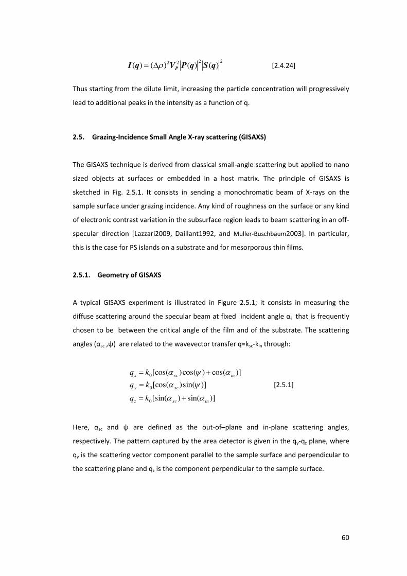
60

2222 )()()()( qSqPVqI P [2.4.24]

Thus starting from the dilute limit, increasing the particle concentration will progressively

lead to additional peaks in the intensity as a function of q.

2.5. Grazing-Incidence Small Angle X-ray scattering (GISAXS)

The GISAXS technique is derived from classical small-angle scattering but applied to nano

sized objects at surfaces or embedded in a host matrix. The principle of GISAXS is

sketched in Fig. 2.5.1. It consists in sending a monochromatic beam of X-rays on the

sample surface under grazing incidence. Any kind of roughness on the surface or any kind

of electronic contrast variation in the subsurface region leads to beam scattering in an off-

specular direction [Lazzari2009, Daillant1992, and Muller-Buschbaum2003]. In particular,

this is the case for PS islands on a substrate and for mesorporous thin films.

2.5.1. Geometry of GISAXS

A typical GISAXS experiment is illustrated in Figure 2.5.1; it consists in measuring the

diffuse s atte i g a ou d the spe ula ea at fi ed i ide t a gle αi that is frequently

chosen to be between the critical angle of the film and of the substrate. The scattering

a gles αsc ,ψ a e elated to the a e e to t a sfe =ksc-kin through:

)]sin()[sin(

)]sin()[cos(

)]cos()cos()[cos(

0

0

0

inscz

scy

inscx

kq

kq

kq

[2.5.1]

He e, αsc a d ψ a e defi ed as the out-of–plane and in-plane scattering angles,

respectively. The pattern captured by the area detector is given in the qy-qz plane, where

qy is the scattering vector component parallel to the sample surface and perpendicular to

the scattering plane and qz is the component perpendicular to the sample surface.

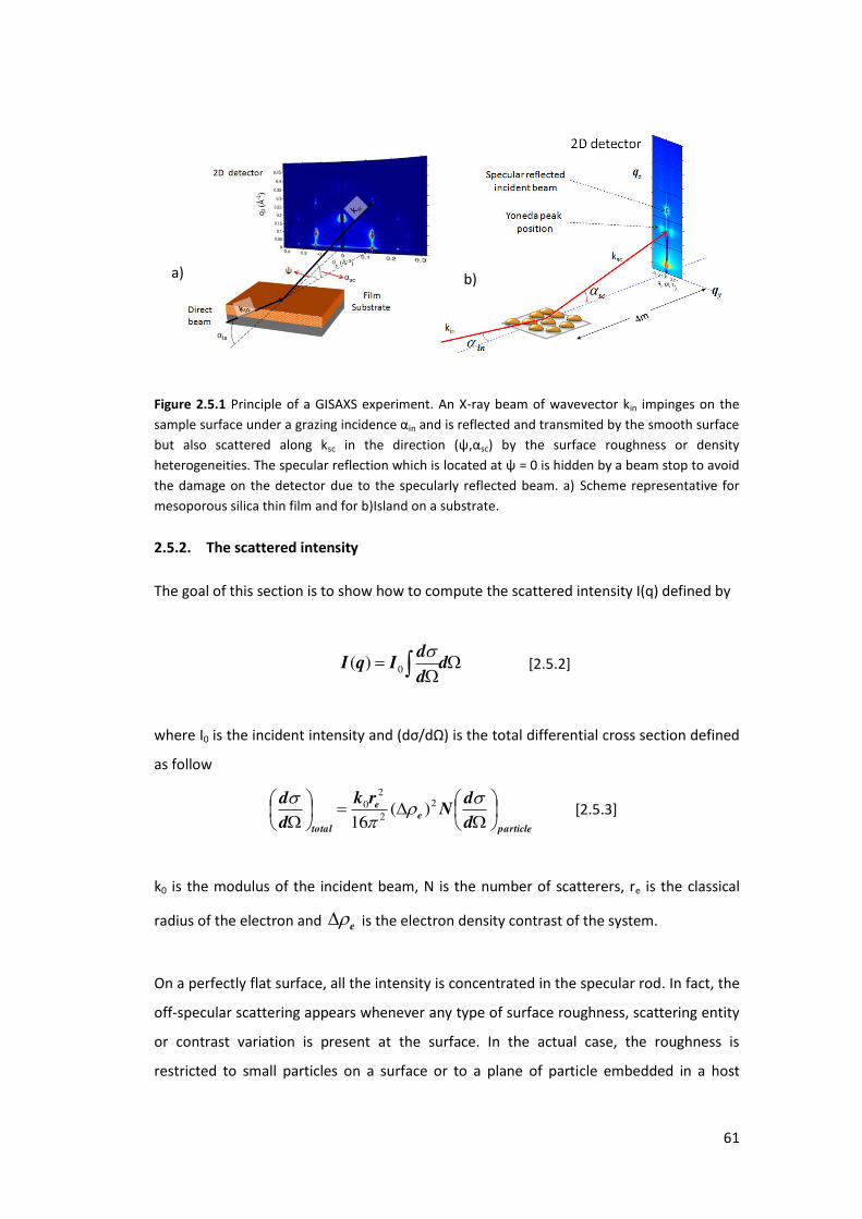
61

Figure 2.5.1 Principle of a GISAXS experiment. An X-ray beam of wavevector kin impinges on the

sa ple su fa e u de a g azi g i ide e αin and is reflected and transmited by the smooth surface

but also scattered along ksc i the di e tio ψ,αsc) by the surface roughness or density

heterogeneities. The specular reflection which is lo ated at ψ = is hidde a ea stop to a oid the damage on the detector due to the specularly reflected beam. a) Scheme representative for

mesoporous silica thin film and for b)Island on a substrate.

2.5.2. The scattered intensity

The goal of this section is to show how to compute the scattered intensity I(q) defined by

dd

dIqI

0)( [2.5.2]

where I0 is the i ide t i te sit a d dσ/dΩ is the total diffe e tial oss se tio defi ed

as follow

particle

ee

total d

dN

rk

d

d

22

20 )(

16 [2.5.3]

k0 is the modulus of the incident beam, N is the number of scatterers, re is the classical

radius of the electron and e is the electron density contrast of the system.

On a perfectly flat surface, all the intensity is concentrated in the specular rod. In fact, the

off-specular scattering appears whenever any type of surface roughness, scattering entity

or contrast variation is present at the surface. In the actual case, the roughness is

restricted to small particles on a surface or to a plane of particle embedded in a host

a) b)

62

matrix with well defined geometrical shapes. Each particle is characterized by its position

on the substrate Ri and its shape function fi(r) equal to one inside the object and zero

outside. The scattering density (electronic density) is given by:

i

ii

e Rrrfr )()()( 0 [2.5.4]

where ⊗ is the otatio fo the o olutio p odu t a d 0 is the mean electronic

density. In the framework of the kinematic approximation, the differential cross section

per particle is proportional to the modulus square of the Fourier transform of the

electronic density. Thus, the differential cross section per a particle and par unit area in an

off-specular direction is given by

22)()()()( qAqSqPq

d

d

particle

[2.5.5]

where P(q) is the form factor of the object and the S(q) represent the interference term

which takes in account the position of objects.

During the course of this thesis, 2 systems have been studied using GISAXS:

- polystyrene islands

- mesoporous silica thin films.

Figure 2.5.2 (a) Islands supported on a substrate (e.g. Polystyrene Island) (b) Particles

encapsulated in an overlayer on a substrate (e.g. Mesoporous silica film)

(a)

(b)

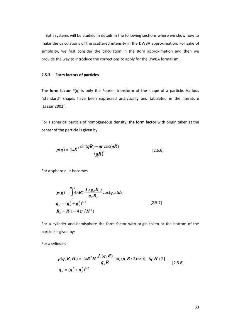
63

Both systems will be studied in details in the following sections where we show how to

make the calculations of the scattered intensity in the DWBA approximation. For sake of

simplicity, we first consider the calculation in the Born approximation and then we

provide the way to introduce the corrections to apply for the DWBA formalism.

2.5.3. Form factors of particles

The form factor P(q) is only the Fourier transform of the shape of a particle. Various

sta da d shapes have been expressed analytically and tabulated in the literature

[Lazzari2002].

For a spherical particle of homogeneous density, the form factor with origin taken at the

center of the particle is given by

33 )cos()sin(

4)(qR

qRqrqRRqp

[2.5.6]

For a spheroid, it becomes

)41(

)(

)cos()(

4)(

22

2/122//

//

//12/

0

2

HzRR

qqq

dzzqRq

RqJRqp

z

yx

z

z

z

H

z

[2.5.7]

For a cylinder and hemisphere the form factor with origin taken at the bottom of the

particle is given by:

For a cylinder:

2/122//

//

//12

)(q

]2/exp[)2/(sin)(

2),,(

yx

zzc

qq

HiqRqRq

RqJHRHRqp

[2.5.8]

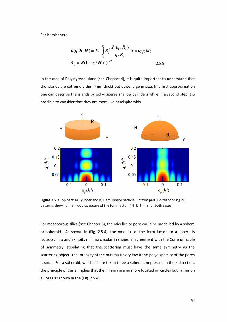
64

For hemisphere:

))/(1(R

)exp()(

2),,(

2/12z

//

//1H

0

2

HzR

dzziqRq

RqJRHRqp z

z

z

z

[2.5.9]

In the case of Polystyrene island (see Chapter 4), it is quite important to understand that

the islands are extremely thin (4nm thick) but quite large in size. In a first approximation

one can describe the islands by polydisperse shallow cylinders while in a second step it is

possible to consider that they are more like hemispheroids.

Figure 2.5.3 Top part: a) Cylinder and b) Hemisphere particle. Bottom part: Corresponding 2D

patterns showing the modulus square of the form factor ( H=R=9 nm for both cases)

For mesoporous silica (see Chapter 5), the micelles or pore could be modelled by a sphere

or spheroid. As shown in (Fig. 2.5.4), the modulus of the form factor for a sphere is

isotropic in q and exhibits minima circular in shape, in agreement with the Curie principle

of symmetry, stipulating that the scattering must have the same symmetry as the

scattering object. The intensity of the minima is very low if the polydispersity of the pores

is small. For a spheroid, which is here taken to be a sphere compressed in the z direction,

the principle of Curie implies that the minima are no more located on circles but rather on

ellipses as shown in the (Fig. 2.5.4).

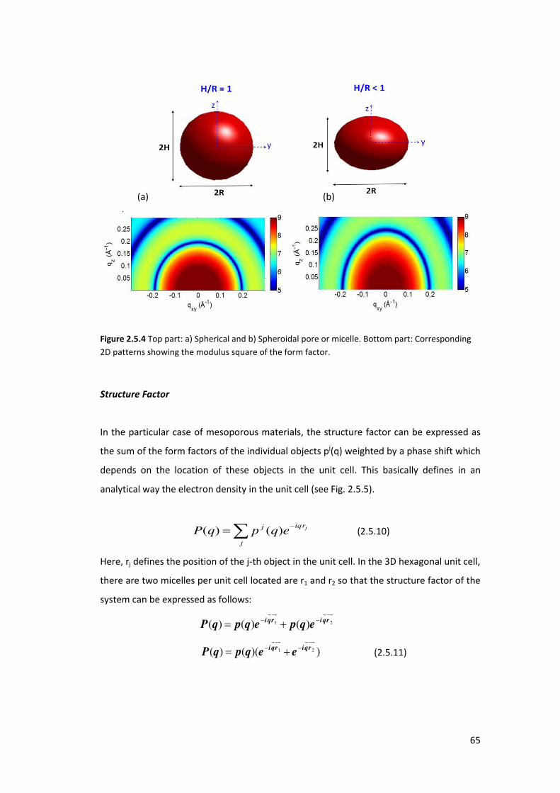
65

Figure 2.5.4 Top part: a) Spherical and b) Spheroidal pore or micelle. Bottom part: Corresponding

2D patterns showing the modulus square of the form factor.

Structure Factor

In the particular case of mesoporous materials, the structure factor can be expressed as

the sum of the form factors of the individual objects pj(q) weighted by a phase shift which

depends on the location of these objects in the unit cell. This basically defines in an

analytical way the electron density in the unit cell (see Fig. 2.5.5).

j

iqrj jeqpqP )()( (2.5.10)

Here, rj defines the position of the j-th object in the unit cell. In the 3D hexagonal unit cell,

there are two micelles per unit cell located are r1 and r2 so that the structure factor of the

system can be expressed as follows:

21 )()()( rqirqieqpeqpqP

))(()( 21 rqirqieeqpqP (2.5.11)

(a) (b)

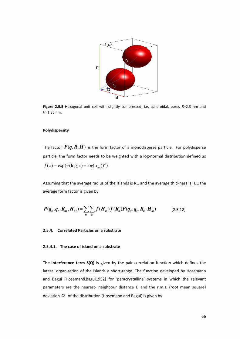
66

Figure 2.5.5 Hexagonal unit cell with slightly compressed, i.e. spheroidal, pores R=2.3 nm and

H=1.85 nm.

Polydispersity

The factor ),,( HRqP is the form factor of a monodisperse particle. For polydisperse

particle, the form factor needs to be weighted with a log-normal distribution defined as

)))log()(log(exp()( 2avxxxf .

Assuming that the average radius of the islands is Rav and the average thickness is Hav, the

average form factor is given by

m k

mkzkmavavz HRqqPRfHfHRqqP ),,,()()(),,,( //// [2.5.12]

2.5.4. Correlated Particles on a substrate

2.5.4.1. The case of island on a substrate

The interference term S(Q) is given by the pair correlation function which defines the

lateral organization of the islands a short-range. The function developed by Hosemann

a d Bagui [Hose a &Bagui ] fo pa a stalli e s ste s i hi h the ele a t

parameters are the nearest- neighbour distance D and the r.m.s. (root mean square)

deviation of the distribution (Hosemann and Bagui) is given by

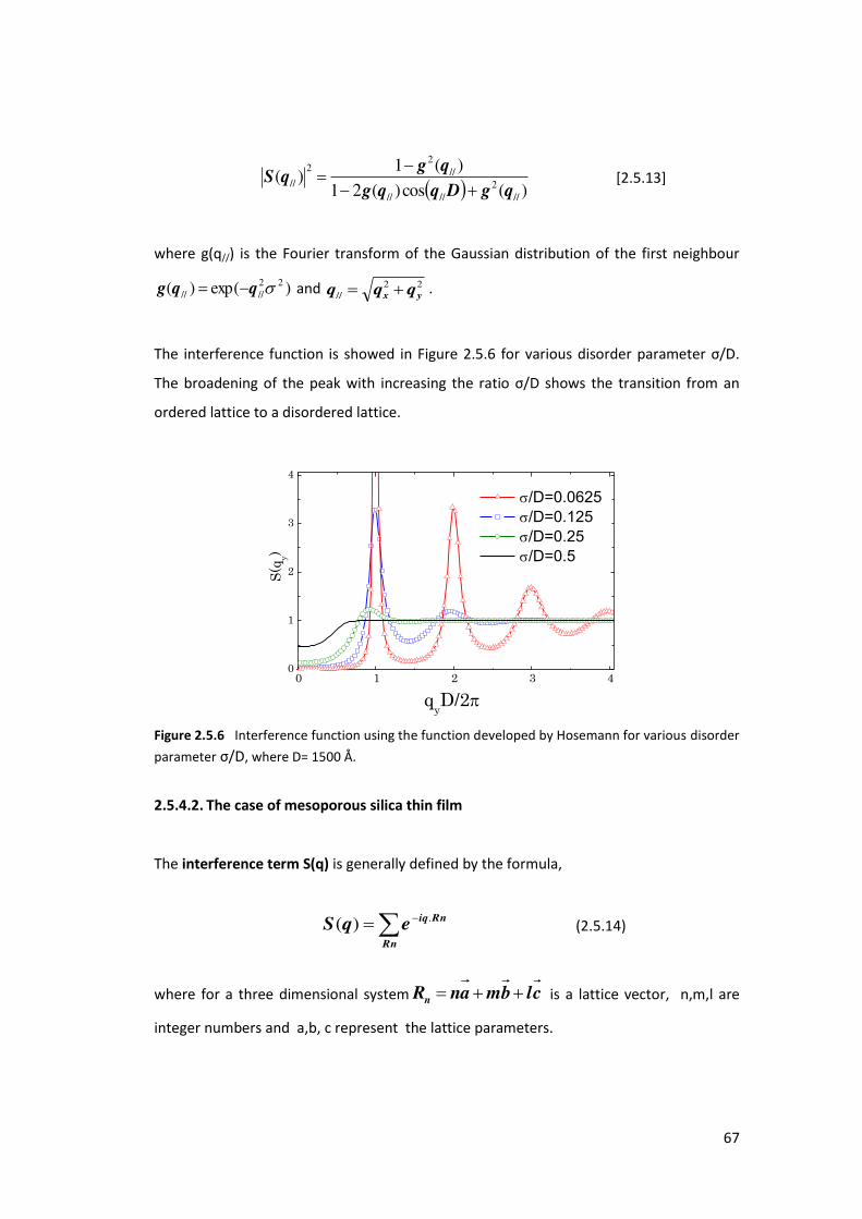
67

)(cos)(21)(1

)(//

2////

//2

2

//qgDqqg

qgqS

[2.5.13]

where g(q//) is the Fourier transform of the Gaussian distribution of the first neighbour

)exp()( 22//// qqg and 22

// yx qqq .

The i te fe e e fu tio is sho ed i Figu e . . fo a ious diso de pa a ete σ/D.

The oade i g of the peak ith i easi g the atio σ/D sho s the t a sitio f o a

ordered lattice to a disordered lattice.

0 1 2 3 40

1

2

3

4

/D=0.0625

/D=0.125

/D=0.25

/D=0.5

S(q

y)

qyD/2

Figure 2.5.6 Interference function using the function developed by Hosemann for various disorder

parameter σ/D, where D= 1500 Å.

2.5.4.2. The case of mesoporous silica thin film

The interference term S(q) is generally defined by the formula,

Rn

RniqeqS .)( (2.5.14)

where for a three dimensional system clbmanRn is a lattice vector, n,m,l are

integer numbers and a,b, c represent the lattice parameters.

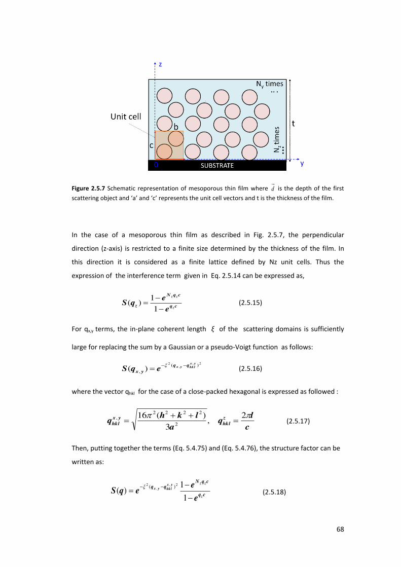
68

Figure 2.5.7 Schematic representation of mesoporous thin film where d is the depth of the first

s atte i g o je t a d a a d ep ese ts the u it ell e to s a d t is the thi k ess of the fil .

In the case of a mesoporous thin film as described in Fig. 2.5.7, the perpendicular

direction (z-axis) is restricted to a finite size determined by the thickness of the film. In

this direction it is considered as a finite lattice defined by Nz unit cells. Thus the

expression of the interference term given in Eq. 2.5.14 can be expressed as,

cq

cqN

zz

zz

e

eqS

1

1)( (2.5.15)

For qx,y terms, the in-plane coherent length ξ of the scattering domains is sufficiently

large for replacing the sum by a Gaussian or a pseudo-Voigt function as follows:

2,,

2 )(, )(

yxhklyx qq

yx eqS

(2.5.16)

where the vector qhkl for the case of a close-packed hexagonal is expressed as followed :

c

lq

a

lkhq z

hkl

yx

hkl

2 ,

3)(16

2

2222,

(2.5.17)

Then, putting together the terms (Eq. 5.4.75) and (Eq. 5.4.76), the structure factor can be

written as:

cq

cqNqq

z

zzyxhklyx

e

eeqS

1

1)(

2,,

2 )( (2.5.18)

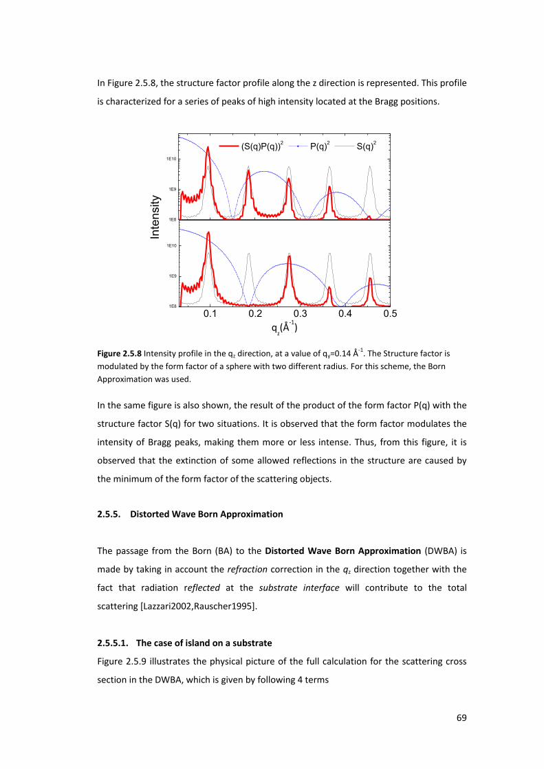
69

In Figure 2.5.8, the structure factor profile along the z direction is represented. This profile

is characterized for a series of peaks of high intensity located at the Bragg positions.

0.1 0.2 0.3 0.4 0.51E8

1E9

1E10

1E8

1E9

1E10

Inte

nsity

qz(Å

-1)

(S(q)P(q))2 P(q)

2 S(q)

2

Figure 2.5.8 Intensity profile in the qz direction, at a value of qy=0.14 Å-1. The Structure factor is

modulated by the form factor of a sphere with two different radius. For this scheme, the Born

Approximation was used.

In the same figure is also shown, the result of the product of the form factor P(q) with the

structure factor S(q) for two situations. It is observed that the form factor modulates the

intensity of Bragg peaks, making them more or less intense. Thus, from this figure, it is

observed that the extinction of some allowed reflections in the structure are caused by

the minimum of the form factor of the scattering objects.

2.5.5. Distorted Wave Born Approximation

The passage from the Born (BA) to the Distorted Wave Born Approximation (DWBA) is

made by taking in account the refraction correction in the qz direction together with the

fact that radiation reflected at the substrate interface will contribute to the total

scattering [Lazzari2002,Rauscher1995].

2.5.5.1. The case of island on a substrate

Figure 2.5.9 illustrates the physical picture of the full calculation for the scattering cross

section in the DWBA, which is given by following 4 terms

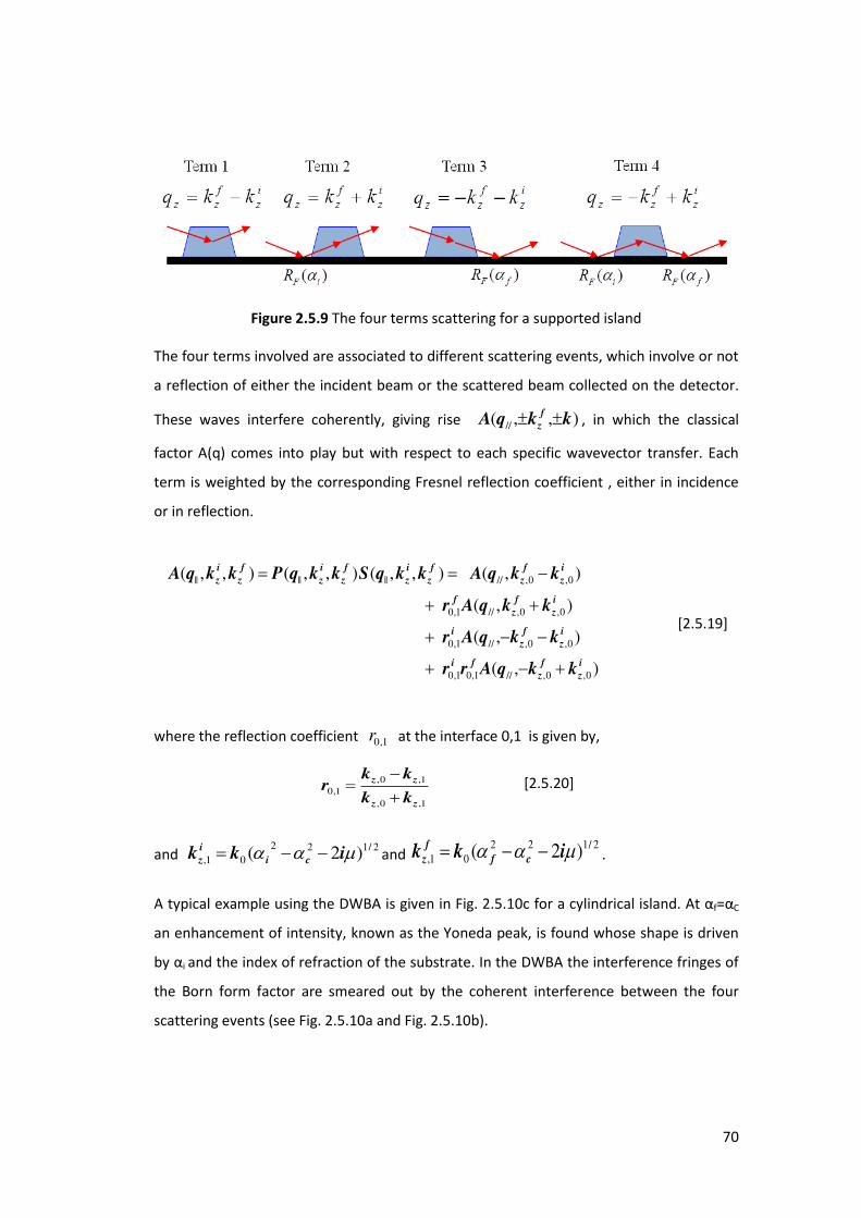
70

Figure 2.5.9 The four terms scattering for a supported island

The four terms involved are associated to different scattering events, which involve or not

a reflection of either the incident beam or the scattered beam collected on the detector.

These waves interfere coherently, giving rise ),,( // kkqA f

z , in which the classical

factor A(q) comes into play but with respect to each specific wavevector transfer. Each

term is weighted by the corresponding Fresnel reflection coefficient , either in incidence

or in reflection.

),(

),(

),(

),( ),,(),,( ),,(

0,0,//1,01,0

0,0,//1,0

0,0,//1,0

0,0,//||||||

i

z

f

z

fi

i

z

f

z

i

i

z

f

z

f

i

z

f

z

f

z

i

z

f

z

i

z

f

z

i

z

kkqArr

kkqAr

kkqAr

kkqAkkqSkkqPkkqA

[2.5.19]

where the reflection coefficient 1,0r at the interface 0,1 is given by,

1,0,

1,0,1,0

zz

zz

kk

kkr

[2.5.20]

and 2/122

01, )2( ikk ci

i

z and 2/122

01, )2( ikk cf

f

z .

A typical example using the DWBA is given in Fig. 2.5.10c for a cylindrical isla d. At αf=αC

an enhancement of intensity, known as the Yoneda peak, is found whose shape is driven

αi and the index of refraction of the substrate. In the DWBA the interference fringes of

the Born form factor are smeared out by the coherent interference between the four

scattering events (see Fig. 2.5.10a and Fig. 2.5.10b).

71

0.04 0.08 0.12 0.1610

-11

10-9

10-7

10-5

10-3

10-1

I1

I2

I3

I4

Re

lative I

nte

nsity

qz(Å-1)

i

c/2

0.05 0.10 0.15

10-13

10-11

10-9

10-7

10-5

10-3

10-1

I1

I2

I3

I4

Re

lative I

nte

nsity

qz(Å-1)

i

c

Figure 2.5.10 The modulus squared of the various component involved in the cylinder DWBA form

factor shown in the eq 2.5.19. The line (black, green, blue, red) correspond respectively, to the four

events of Fig. 2.5.9 f o left to ight. Whe a αi=αc/ αi= αc. (c) Form factor of a cylindrical

isla d i ludi g all the fou te of s atte i g ith a i ide e a gle αi=αc and considering that

S(q)=1, R=H=9nm .

If the substrate is covered with a continuous layer of thickness t as e sho i Figu e

2.5.11,

Figure 2.5.11 Island supported on a layer on a substrate

the reflection coefficient in the Eq. 2.2.66 becomes:

)2exp(1

)2exp(

2,11,0

2,11,0

tikrr

tikrrR

z

z

where ,,

,,,

jziz

jziz

jikk

kkr

[2.5.21]

(b) (a)

(c)

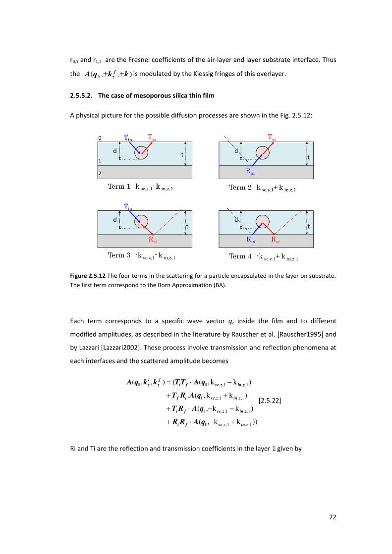
72

r0,1 and r1,2 are the Fresnel coefficients of the air-layer and layer substrate interface. Thus

the ),,( // kkqA f

z is modulated by the Kiessig fringes of this overlayer.

2.5.5.2. The case of mesoporous silica thin film

A physical picture for the possible diffusion processes are shown in the Fig. 2.5.12:

Figure 2.5.12 The four terms in the scattering for a particle encapsulated in the layer on substrate.

The first term correspond to the Born Approximation (BA).

Each term corresponds to a specific wave vector qz inside the film and to different

modified amplitudes, as described in the literature by Rauscher et al. [Rauscher1995] and

by Lazzari [Lazzari2002]. These process involve transmission and reflection phenomena at

each interfaces and the scattered amplitude becomes

))kk,(

)kk,(

)kk,(.

)kk,((),,(

1,,1,,||

1,,1,,||

1,,1,,||

1,,1,,||||

zinzscfi

zinzscfi

zinzscif

zinzscfi

f

z

i

z

qARR

qART

qART

qATTkkqA

[2.5.22]

Ri and Ti are the reflection and transmission coefficients in the layer 1 given by

73

tikscasca

sca

ftikscasca

tikscasca

f

tikinin

in

itikinin

tikinin

i

zscazsca

zsca

zinzin

zin

err

tT

err

ertR

err

tT

err

ertR

1,,1,,

1,,

1,,1,,

1,,

22,11,0

1,02

2,11,0

22,11,0

22,11,0

1,02

2,11,0

22,11,0

1 ,

1

1 ,

1

[2.5.23]

in which t is the thickness of the film, with kin,z,1 and ksc,z,1 are the z-axis component of the

incident and scattered wave vector in medium 1, 1

21,

201,, 2 iczin kk ,

12

1,2

01,, 2kk iczsc i hi h αc,1 is the iti al a gle of the fil a d β1 the absorption in

the film. The coefficients ri,j and ti,j are the Fresnel coefficients at the interface between

two media i and j and are defined by

jzinizin

izinin

ji

jzinizin

jzinizinin

jikk

kt

kk

kkr

,,,,

,,,

,,,,

,,,,,

2 ,

[2.5.24]

Similar relationships hold for the scattered values.

2.6. Coherent X-ray Diffraction Imaging (CXDI)

CXDI is a new technique promising for high resolution lens-less imaging of non-crystalline

and biological microscopic specimens. In CXDI, a fully coherent beam of x-rays is

impinging on a single particle whose dimension is typically of the order of the µm. If the

incident plane wave encounters some heterogeneities inside the particle like voids, grains

or even a rough surface, a speckle pattern is measured in the far-field region. The speckle

pattern arises from the interferences between all the scattering heterogeneities. It is

characterized by a large number of small spots with no apparent periodicity. The speckle

is thus the signature of a non uniform object and it is therefore particularly tempting to

unravel its structure. This is a difficult task as in all scattering processes, the phase which

is a key parameter to locate the position of the heterogeneities inside a scattering object

is lost. The only information that remains in the scattering pattern is the modulus square

of the scattered amplitude. However, it has been shown that when the diffraction pattern

is sampled twice finer than the Nyquist frequency, the phase can be recovered using an

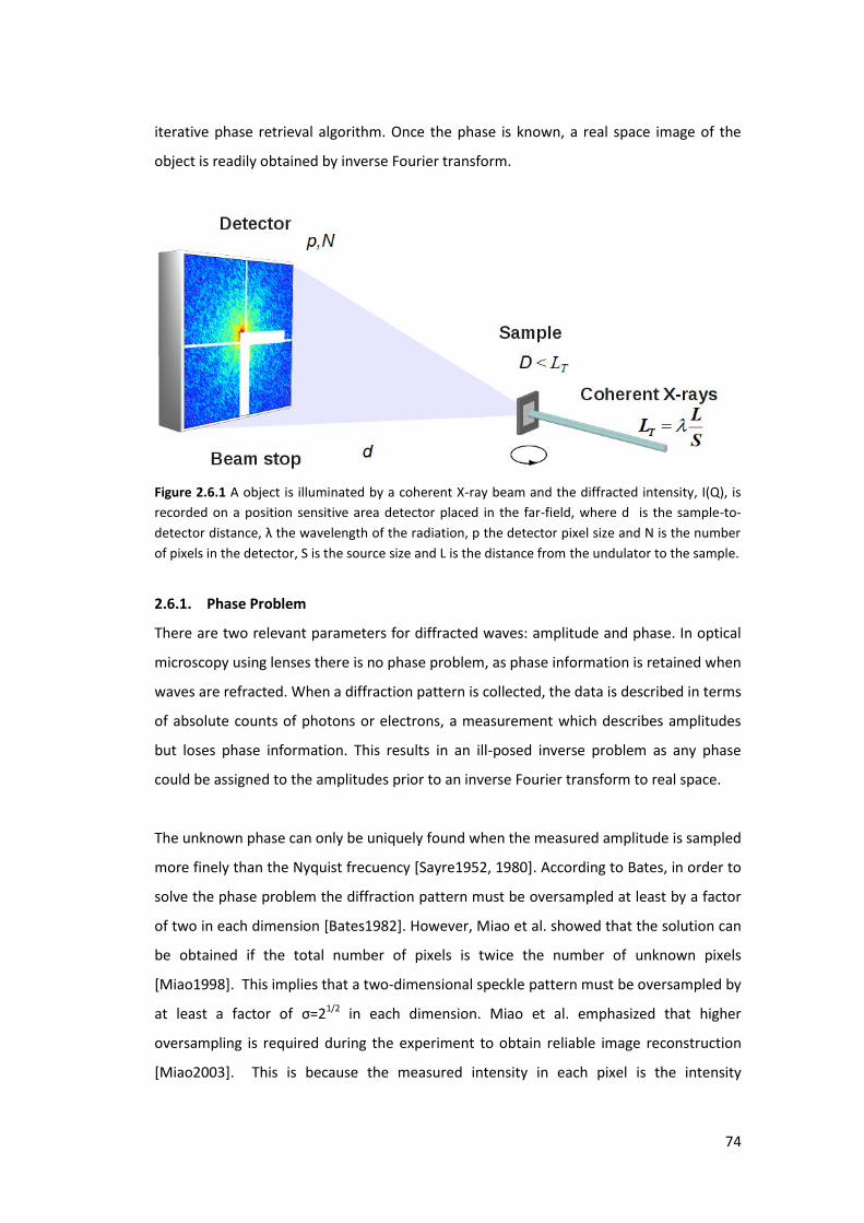
74

iterative phase retrieval algorithm. Once the phase is known, a real space image of the

object is readily obtained by inverse Fourier transform.

Figure 2.6.1 A object is illuminated by a coherent X-ray beam and the diffracted intensity, I(Q), is

recorded on a position sensitive area detector placed in the far-field, where d is the sample-to-

dete to dista e, the a ele gth of the adiatio , p the dete to pi el size a d N is the u e of pixels in the detector, S is the source size and L is the distance from the undulator to the sample.

2.6.1. Phase Problem

There are two relevant parameters for diffracted waves: amplitude and phase. In optical

microscopy using lenses there is no phase problem, as phase information is retained when

waves are refracted. When a diffraction pattern is collected, the data is described in terms

of absolute counts of photons or electrons, a measurement which describes amplitudes

but loses phase information. This results in an ill-posed inverse problem as any phase

could be assigned to the amplitudes prior to an inverse Fourier transform to real space.

The unknown phase can only be uniquely found when the measured amplitude is sampled

more finely than the Nyquist frecuency [Sayre1952, 1980]. According to Bates, in order to

solve the phase problem the diffraction pattern must be oversampled at least by a factor

of two in each dimension [Bates1982]. However, Miao et al. showed that the solution can

be obtained if the total number of pixels is twice the number of unknown pixels

[Miao1998]. This implies that a two-dimensional speckle pattern must be oversampled by

at least a factor of σ= 1/2 in each dimension. Miao et al. emphasized that higher

oversampling is required during the experiment to obtain reliable image reconstruction

[Miao2003]. This is because the measured intensity in each pixel is the intensity

75

integrated over the solid angle defined by the detector pixel size. The measured intensity

at low oversampling ratios can deviate substantially from the exact sampled data [Song

2007].

A representative example about the importance of the phase value in the image

reconstruction process is shown in Figure 2.6.2. In this figure, it is possible to observe the

problem linked to the phase loss which makes impossible the image reconstruction from a

diffraction pattern (see Figure 2.6.2a). When a good phase is associated to the amplitude

information is possible to reconstruct the diffracted object (see Figure 2.6.2 b).

Figure 2.6.2 The importance of the phase on the reconstruction of the image

2.6.2. Phase Retrieval Method

In a typical reconstruction [Vartanyants2005] the first step is to generate random phases

ϕ(q) and to combine them with the amplitude information A(q) from the reciprocal space

pattern. Then a Fourier transform is applied back and forth to move between real space

and reciprocal space with the modulus squared of the diffracted wave field set equal to

the measured diffraction intensities at each cycle. By applying various constraints in real

and reciprocal space the pattern evolves into an image after enough iterations of the

b) Object Projection of object

FTT of the projection of

object

FTT inversion of amplitude with

phase

a) Object Projection of object

FTT of the projection of

object

FTT inversion of amplitude

without phase

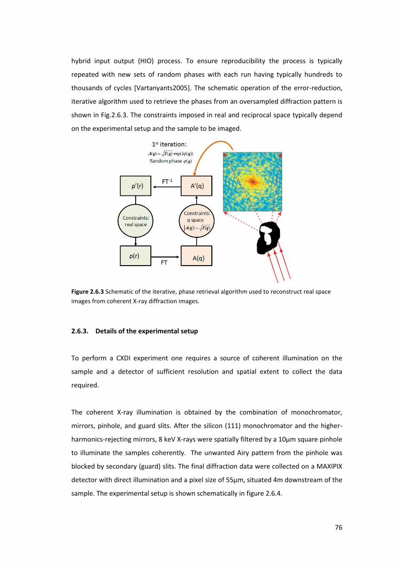
76

hybrid input output (HIO) process. To ensure reproducibility the process is typically

repeated with new sets of random phases with each run having typically hundreds to

thousands of cycles [Vartanyants2005]. The schematic operation of the error-reduction,

iterative algorithm used to retrieve the phases from an oversampled diffraction pattern is

shown in Fig.2.6.3. The constraints imposed in real and reciprocal space typically depend

on the experimental setup and the sample to be imaged.

Figure 2.6.3 Schematic of the iterative, phase retrieval algorithm used to reconstruct real space

images from coherent X-ray diffraction images.

2.6.3. Details of the experimental setup

To perform a CXDI experiment one requires a source of coherent illumination on the

sample and a detector of sufficient resolution and spatial extent to collect the data

required.

The coherent X-ray illumination is obtained by the combination of monochromator,

mirrors, pinhole, and guard slits. After the silicon (111) monochromator and the higher-

harmonics-rejecting mirrors, 8 keV X-rays were spatially filtered by a 10µm square pinhole

to illuminate the samples coherently. The unwanted Airy pattern from the pinhole was

blocked by secondary (guard) slits. The final diffraction data were collected on a MAXIPIX

detector with direct illumination and a pixel size of 55µm, situated 4m downstream of the

sample. The experimental setup is shown schematically in figure 2.6.4.

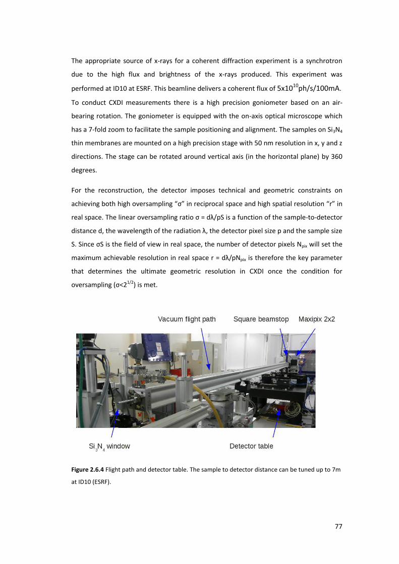
77

The appropriate source of x-rays for a coherent diffraction experiment is a synchrotron

due to the high flux and brightness of the x-rays produced. This experiment was

performed at ID10 at ESRF. This beamline delivers a coherent flux of 5x1010ph/s/100mA.

To conduct CXDI measurements there is a high precision goniometer based on an air-

bearing rotation. The goniometer is equipped with the on-axis optical microscope which

has a 7-fold zoom to facilitate the sample positioning and alignment. The samples on Si3N4

thin membranes are mounted on a high precision stage with 50 nm resolution in x, y and z

directions. The stage can be rotated around vertical axis (in the horizontal plane) by 360

degrees.

For the reconstruction, the detector imposes technical and geometric constraints on

achieving both high oversampling σ in reciprocal space and high spatial resolution in

real space. The linear o e sa pli g atio σ = d /p“ is a fu tio of the sa ple-to-detector

distance d, the a ele gth of the adiatio , the detector pixel size p and the sample size

S. Since σS is the field of view in real space, the number of detector pixels Npix will set the

maximum achievable esolutio i eal spa e = d /pNpix is therefore the key parameter

that determines the ultimate geometric resolution in CXDI once the condition for

oversampling σ< 1/2) is met.

Figure 2.6.4 Flight path and detector table. The sample to detector distance can be tuned up to 7m

at ID10 (ESRF).

78

79

Bibliography [Als-Nielsen&McMorrow2010] Als-Nielsen, J.; McMorrow, D. Elements of Modern X-Ray Physics.

John Wiley & Sons, New York, 2nd edition, 2010.

[Bale-Schmidt 1984] Bale, H.D.; Schmidt, P.W. Phys. Rev. Lett. (1994)53, 596-599.

[Bates1982] Bates, R. H. T. Optik, (1982) 61, 247–262.

[Born&Wolf1980] Born, M.; Wolf, E. Principles of Optics, Oxford: Pergamon Press, 1980.

[Daillant1992] Daillant, J.; Belorgey O., J. Chem. Phys. (1992) 97, 5824-5835.

[Gibaud2009] Gibaud, A. Specular Reflectivity from Smooth and Rough Surfaces, X Ray and

Neutron Reflectivity: Principle and Applications, Edited by Daillant, J. and Gibaud, A. (Springer,

Paris 2009), pp 133-182.

[Debye&Bueche1949] Debye, P.; Bueche, A. M., J. Appl. Phys. (1949) 20, 518.

[Glatter1982] Glatter, O; and Krattky, O., Small Angle x-ray scattering, Academic Press London,

1982.

[Guinier1955] Guinier A.; Fournet, G., Small Angle sacttering of x-rays Wiley , 1955.

[Hamley1994] Hamley, I. W; Pedersen, J. S., J. Appl. Crystallogr. (1994) 27, 29.

[Hoseman&Bagui1952] Hosemann, R.; Baghi, S. N., Acta Crystallogr. (1952) 5, 612.

[Lazzari2002] Lazzari, R. J. Appl. Crystallogr. (2002) 35, 406-421.

[Lazzari2009] Lazzari, R. Grazing Incidence Small-Angle X-Ray Scattering from Nanostructures, X

Ray and Neutron Reflectivity: Principle and Applications, Edited by Daillant, J. and Gibaud, A.

(Springer, Paris 2009), pp 283-344.

[Miao1998] Miao, J.; Sayre, D. ; Chapman, H. N. J. Opt. Soc. Am. A (1998) 15,1662–1669.

[Miao2003] Miao, J.; Ishikawa, T.; Anderson, E. H. Phys. Rev. B (2003) 67,174104.

[Mulller-Buschbaum2003] Muller-Buschbaum, P. Analytical and Bioanalytical Chemistry (2003)

376(1):310.

[Parrat1954] Parrat, L.G., Phys. Rev. (1954) 95, 359.

[Rauscher1995] Rauscher M.; Salditt T.; and Spohn H. Phys. Rev. B (1995) 52(23), 16855-16863.

[Roentgen1896] W. C. Roentgen. Nature (1896) 53:274-276.

[Sayre1952] Sayre, D. Acta Cryst. (1952) 5: 843.

[Sayre1980] Sayre, D. Imaging Processes and Coherence in Physics. Lecture Notes in Physics, Vol.

112, edited by M. Schlenker, M. Fink, J.-P. Goedgebuer, C. Malgrange, J.-C. Vienot & R. H. Wade,

pp. 229–235. Heidelberg: Springer, 1980.

[Song2007] Song, C.; Ramunno-Johnson, D.; Nishino, Y.; Kohmura, Y.; Ishikawa, T.; Chen, C. C.; Lee,

T. K.; Miao, J. Phys. Rev. B (2007) 75, 012102.

[Svergun1994] Svergun, D.I., Acta Cryst A (1994) 50, 391-402.

80

[Vartanyants2005] Vartanyants, I.A.; Robinson, I.K.; Onken, J.D.; Pfeifer, M.A.; Williams, G.J.;

Pfeiffer, F.; Metzger, H.; Zhong, Z. ; G. Bauer, Phys. Rev. B (2005) 71: 245302.

81

CHAPTER 3

3. Analysis of porous powder of CaCO3 prepared via sc-CO2

using Small Angle X-ray Scattering

In this chapter, the results of Small Angle and Ultra Small Angle X-ray Scattering on porous

CaCO3 microparticles of pulverulent vaterite made by a conventional chemical route and

by supercritical CO2 are presented. The scattering curves are analyzed in the framework of

the Guinier-Porod model which gives the radii of gyration of the scattering objects and

their fractal dimension. In addition, we determine the porosity and the specific surface

area by using the Porod invariant which is modified to take in account the effective

thickness of the pellet. The results of this analysis are compared to the ones obtained by

nitrogen adsorption.

In addition, we also show the first results of Coherent Diffraction Imaging (CDI)

experiments performed at the ID10A beam line on single particles of vaterite.

Mate ial i this hapte appea s i the pape A al sis of po ous po de of CaCO3

prepared via sc-CO2 using Small Angle X- a “ atte i g E. A. Cha ez Panduro, T. Beuvier,

M. Fernandez Martinez, L. Hassani, B. Calvignac, F. Boury, A. Gibaud, Journal of Applied

Crystallography 01/2012; 45.

82

3.1. Introduction

Small-angle x-ray scattering (SAXS) is nowadays one of the very few techniques that can

provide statistical information about the morphology, porosity and specific surface area of

materials at the nanometer scale. Among the most studied materials by this technique for

which there is an abundant literature on the topics one finds coal powders [Gibaud.1996,

Radlinski2004, Schmidt1982, Kalliat1981]. For extracting all the information, it is

important to measure the scattered intensity in absolute units which in turn necessitates

to correct the measured intensity from the transmission coefficient and from the

thickness of the material. This is one of the major problem to solve when one wants to

analyze the data obtained from powders since i) the transmitted beam intensity decays

exponentially with the thickness of the sample and ii) the real thickness can be difficult to

ascertain when one is dealing with powdered samples. The analysis of the data strongly

depends on how the experiment has been performed and how much effort the analyst

wants to put into the model. For many years, many researchers were satisfied with

standard analysis through linear plots such as Guinier or Porod plots

[Guinier&Fournet1955, Glatter&Kratky1982]. Nonlinear least-s ua es fits i hi h the

electron density was refined, were then introduced to analyze the data

[Feigin&Svergun1987].

Guinier and Porod plots are the basic starting points for reaching immediate information

about the particle size (radius of gyration) and about scattering inhomogeneities through

the Porod exponent, i.e. the slope of the scattering curve in a log-log representation. A

Porod exponent of 4, points to particles with smooth surfaces while an exponent of 3,

points to very ough su fa es. A e po e t a also poi t to s atte i g f o ollapsed

pol e hai s i a ad sol e t a d e po e t of / poi ts to s atte i g f o full

s olle hai s i a good sol e t . A e po e t of a ep ese t s atte i g eithe f o

Gaussian polymer chains or from a two-dimensional structure (such as lamellae or

platelets).

Although this is quite basic, there are still some improvements on the way to analyze the

data through this type of modelling. In particular, Beaucage wrote in 1994

[Beaucage1994] a paper in which he was showing how to combine the two approaches

into a unified version. This approach is widely used nowadays but it was found that

sometimes it yields unrealistic values for the Porod exponent. This is why

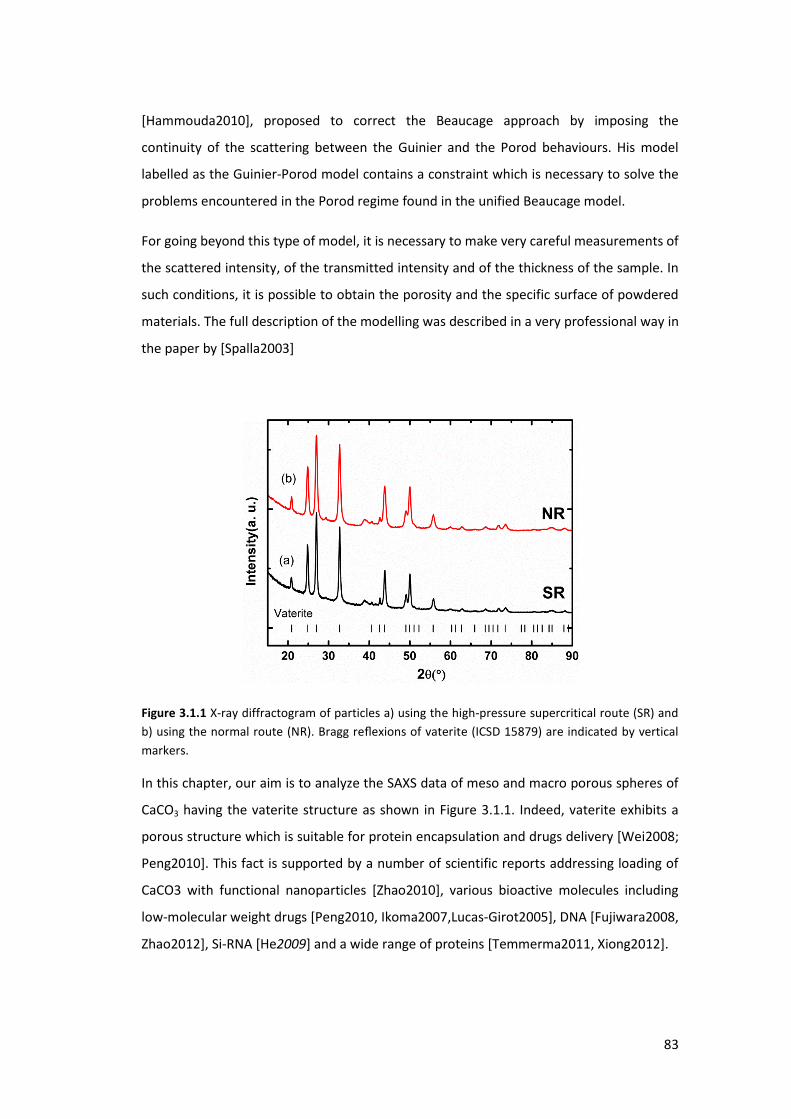
83

[Hammouda2010], proposed to correct the Beaucage approach by imposing the

continuity of the scattering between the Guinier and the Porod behaviours. His model

labelled as the Guinier-Porod model contains a constraint which is necessary to solve the

problems encountered in the Porod regime found in the unified Beaucage model.

For going beyond this type of model, it is necessary to make very careful measurements of

the scattered intensity, of the transmitted intensity and of the thickness of the sample. In

such conditions, it is possible to obtain the porosity and the specific surface of powdered

materials. The full description of the modelling was described in a very professional way in

the paper by [Spalla2003]

Figure 3.1.1 X-ray diffractogram of particles a) using the high-pressure supercritical route (SR) and

b) using the normal route (NR). Bragg reflexions of vaterite (ICSD 15879) are indicated by vertical

markers.

In this chapter, our aim is to analyze the SAXS data of meso and macro porous spheres of

CaCO3 having the vaterite structure as shown in Figure 3.1.1. Indeed, vaterite exhibits a

porous structure which is suitable for protein encapsulation and drugs delivery [Wei2008;

Peng2010]. This fact is supported by a number of scientific reports addressing loading of

CaCO3 with functional nanoparticles [Zhao2010], various bioactive molecules including

low-molecular weight drugs [Peng2010, Ikoma2007,Lucas-Girot2005], DNA [Fujiwara2008,

Zhao2012], Si-RNA [He2009] and a wide range of proteins [Temmerma2011, Xiong2012].

84

Currently, the group of F. Boury (INSERM - Angers) is investigating on direct encapsulation

of a model protein, lyzozyme, into CaCO3 microparticules using sc-CO2 process. They

compared two different approaches for direct encapsulation. In the first approach,

lysozyme was entrapped during the growth of CaCO3 particles in supercritical (SR) CO2,

and in aqueous medium in the second one (called normal route (NR)). It is therefore

important for potential application to understand the morphology of such host matrix and

to see how the synthesis affects the porosity. The samples are powdered samples of

vaterite which are analyzed at small and ultra small angles at the ID02 beam line of ESRF.

They exhibit beautiful scattering patterns arising from the hierarchical architectures

observed in the microspheres of vaterite shown in the Scanning Electron Microscopy

Figure 3.1.2. The inner structure of the CaCO3 microparticles can be unravelled after

grinding the particles in a mortar [Beuvier2010] or by cutting them by a focused ion beam

(FIB) [Suzuki2006]. In order to access the internal structure of particles, powder was

pressed at 240 MPa and the pellet was cut in small pieces. The slide containing many

broken particles was subsequently analysed by SEM. The size distributions were

determined by measuring the diameter of about 200 particles. As shown in Figures 3.1.2a

and 3.2b, the microspheres made by the normal route (NR) have an average diameter of

2.3±1.0 µm. They are composed of agglomerated nanograins. Figures 3.1.2c, 3.1.2d and

3.1.2e show the morphology of the broken particles. Radial fibrous units are observed

with an important macroporosity at the cores of the particles. There is no sign of any

hollow core in such particles.

On the contrary, particles made by the supercritical route (SR) have a higher diameter

(4.9±1.0 µm) (Figure 3.1.2f). The surface and the inner part of the particles look more

compact than the ones of particles made by NR (Figures 3.1.2g and 3.1.2h). This should

likely affect the porosity. Moreover particles made by SR have a hollow core with an

average diameter of 0.7 µm (Figure 3.1.2h). Bigger particles display a larger core (Figure

3.1.2i).

As the distribution and sizes of the macro- and meso-pores in the CaCO3 particles may

differ from one particle to one another, it is very difficult to analytically model the SAXS

data. Therefo e, e ha e used i this a al sis oth [Ha ouda ] a d [“palla ] s

approaches to extract real space information contained in the scattering curves. In the

SAXS analysis, we first apply the Guinier-Porod model and then we use the Porod

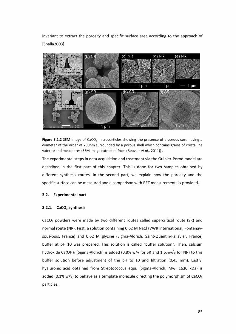
85

invariant to extract the porosity and specific surface area according to the approach of

[Spalla2003]

Figure 3.1.2 SEM image of CaCO3 microparticles showing the presence of a porous core having a

diameter of the order of 700nm surrounded by a porous shell which contains grains of crystalline

vaterite and mesopores (SEM image extracted from (Beuvier et al., 2011)) .

The experimental steps in data acquisition and treatment via the Guinier-Porod model are

described in the first part of this chapter. This is done for two samples obtained by

different synthesis routes. In the second part, we explain how the porosity and the

specific surface can be measured and a comparison with BET measurements is provided.

3.2. Experimental part

3.2.1. CaCO3 synthesis

CaCO3 powders were made by two different routes called supercritical route (SR) and

normal route (NR). First, a solution containing 0.62 M NaCl (VWR international, Fontenay-

sous-bois, France) and 0.62 M glycine (Sigma-Aldrich, Saint-Quentin-Fallavier, France)

buffer at pH 10 was prepared. This solution is called "buffer solution". Then, calcium

hydroxide Ca(OH)2 (Sigma-Aldrich) is added (0.8% w/v for SR and 1.6%w/v for NR) to this

buffer solution before adjustment of the pH to 10 and filtration (0.45 mm). Lastly,

hyaluronic acid obtained from Streptococcus equi. (Sigma-Aldrich, Mw: 1630 kDa) is

added (0.1% w/v) to behave as a template molecule directing the polymorphism of CaCO3

particles.

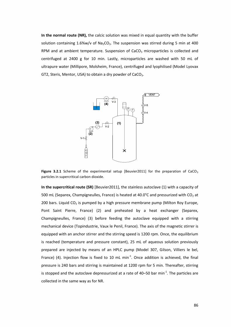
86

In the normal route (NR), the calcic solution was mixed in equal quantity with the buffer

solution containing 1.6%w/v of Na2CO3. The suspension was stirred during 5 min at 400

RPM and at ambient temperature. Suspension of CaCO3 microparticles is collected and

centrifuged at 2400 g for 10 min. Lastly, microparticles are washed with 50 mL of

ultrapure water (Millipore, Molsheim, France), centrifuged and lyophilised (Model Lyovax

GT2, Steris, Mentor, USA) to obtain a dry powder of CaCO3.

Figure 3.2.1 Scheme of the experimental setup [Beuvier2011] for the preparation of CaCO3

particles in supercritical carbon dioxide.

In the supercritical route (SR) [Beuvier2011], the stainless autoclave (1) with a capacity of

500 mL (Separex, Champigneulles, France) is heated at 40.0°C and pressurized with CO2 at

200 bars. Liquid CO2 is pumped by a high pressure membrane pump (Milton Roy Europe,

Pont Saint Pierre, France) (2) and preheated by a heat exchanger (Separex,

Champigneulles, France) (3) before feeding the autoclave equipped with a stirring

mechanical device (Topindustrie, Vaux le Penil, France). The axis of the magnetic stirrer is

equipped with an anchor stirrer and the stirring speed is 1200 rpm. Once, the equilibrium

is reached (temperature and pressure constant), 25 mL of aqueous solution previously

prepared are injected by means of an HPLC pump (Model 307, Gilson, Villiers le bel,

France) (4). Injection flow is fixed to 10 mL min-1. Once addition is achieved, the final

pressure is 240 bars and stirring is maintained at 1200 rpm for 5 min. Thereafter, stirring

is stopped and the autoclave depressurized at a rate of 40–50 bar min-1. The particles are

collected in the same way as for NR.

87

In both cases, powder is placed in a cell closed by 2 kapton windows with a thickness of 50

µm separated by 1.5 mm. The powder is therefore not compressed in the cell.

3.2.2. Methods

SAXS and ultra-small-angle X-rays (USAXS) measurements were performed at the High

Brilliance beamline (ID02) at the ESRF. For the SAXS experiments, a highly collimated

monochromatic x- a ea of a ele gth = . Å passed th ough the pellet a d the

scattered intensity was recorded by an image intensified charge coupled device (CCD)

based x-ray detector (FReLoN) housed in an evacuated flight tube. The measurements

were performed to detector distance of 2 m and typical acquisition time ranged from 0.1

to 0.3 s. The measured two-dimensional SAXS patterns were normalized to an absolute

scale, azimuthally averaged, and background subtracted to obtain the scattered intensity

I as a fu tio of s atte i g e to , = / si θ/ , he e θ is the s atte i g a gle.

USAXS experiments were carried out in a Bonse-Hart (BH) configuration, which involves a

multiple bounce crossed-analyzer. The set-up provides a useful q range of 10-3<q<1 nm-1

at 12.4 keV. The instrumental background is significantly reduced using specially

fabricated analyzer crystals which allowed us to measure scattered intensities down to

. − . The two sets of experiments, SAXS and USAXS, were overlapped in order to

obtain a complete scattering curve, from q = 0.001 to q = 1 nm-1.

3.3. Morphologic study of CaCO3 particles by SAXS

3.3.1. The GUINIER-POROD model

The elementary analysis of the data consisting in determining the radii of gyration and

fractal dimension of the scattering objects was carried out using the Guinier-Porod model

proposed by [Hammouda2010]. A more elaborated analysis in which the porosity and the

specific surface area were determined, was then performed using the approach

developed by [Spalla2003]. Let us first consider the Guinier-Porod Model.

It is well known since the pioneering work of A. Guinier [Guinier&Fournet1955] that at

very small angles of incidence and provided that the condition qRg << 1 is fulfilled, SAXS

data decrease exponentially as3/22

gRqe

. This behaviour is generally limited to very small

angles of incidence. The range of validity fundamentally depends on the radius of gyration

of the s atte i g pa ti le. Be o d the Gui ie egi e, i.e. fo ‘g >>1 (Porod'regime), a

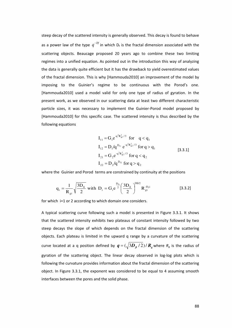
88

steep decay of the scattered intensity is generally observed. This decay is found to behave

as a power law of the type Df

q

in which Df is the fractal dimension associated with the

scattering objects. Beaucage proposed 20 years ago to combine these two limiting

regimes into a unified equation. As pointed out in the introduction this way of analyzing

the data is generally quite efficient but it has the drawback to yield overestimated values

of the fractal dimension. This is why [Hammouda2010] an improvement of the model by

i posi g to the Gui ie s egi e to e o ti uous ith the Po od s o e.

[Hammouda2010] used a model valid for only one type of radius of gyration. In the

present work, as we observed in our scattering data at least two different characteristic

particle sizes, it was necessary to implement the Guinier-Porod model proposed by

[Hammouda2010] for this specific case. The scattered intensity is thus described by the

following equations

2D

222

23/Rq-

221

13/Rq-D

112

13/R-q

111

q qfor /qD I

qqfor eG I

q qfor e /qD I

qqfor eG I

f2

22

2

22

2f1

21

2

g

g

g

[3.3.1]

where the Guinier and Porod terms are constrained by continuity at the positions

iD-gi

Dfi/2

fi2

D

iifi

gii

f

fi

R2

3DeGD with

2

3D

R1

q

[3.3.2]

for which i=1 or 2 according to which domain one considers.

A typical scattering curve following such a model is presented in Figure 3.3.1. It shows

that the scattered intensity exhibits two plateaus of constant intensity followed by two

steep decays the slope of which depends on the fractal dimension of the scattering

objects. Each plateau is limited in the upward q range by a curvature of the scattering

curve located at a q position defined by gfi RDq /)2/3( where Rg is the radius of

gyration of the scattering object. The linear decay observed in log-log plots which is

following the curvature provides information about the fractal dimension of the scattering

object. In Figure 3.3.1, the exponent was considered to be equal to 4 assuming smooth

interfaces between the pores and the solid phase.

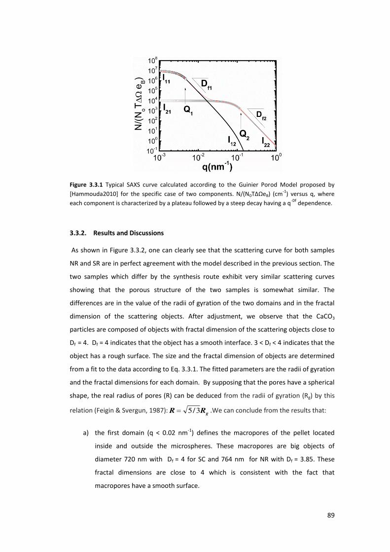
89

Figure 3.3.1 Typical SAXS curve calculated according to the Guinier Porod Model proposed by

[Hammouda2010] for the specific case of two components. N/(N0TΔΩeB) (cm-1) versus q, where

each component is characterized by a plateau followed by a steep decay having a q-Df dependence.

3.3.2. Results and Discussions

As shown in Figure 3.3.2, one can clearly see that the scattering curve for both samples

NR and SR are in perfect agreement with the model described in the previous section. The

two samples which differ by the synthesis route exhibit very similar scattering curves

showing that the porous structure of the two samples is somewhat similar. The

differences are in the value of the radii of gyration of the two domains and in the fractal

dimension of the scattering objects. After adjustment, we observe that the CaCO3

particles are composed of objects with fractal dimension of the scattering objects close to

Df = 4. Df = 4 indicates that the object has a smooth interface. 3 < Df < 4 indicates that the

object has a rough surface. The size and the fractal dimension of objects are determined

from a fit to the data according to Eq. 3.3.1. The fitted parameters are the radii of gyration

and the fractal dimensions for each domain. By supposing that the pores have a spherical

shape, the real radius of pores (R) can be deduced from the radii of gyration (Rg) by this

relation (Feigin & Svergun, 1987):gRR 3/5 .We can conclude from the results that:

a) the first domain (q < 0.02 nm-1) defines the macropores of the pellet located

inside and outside the microspheres. These macropores are big objects of

diameter 720 nm with Df = 4 for SC and 764 nm for NR with Df = 3.85. These

fractal dimensions are close to 4 which is consistent with the fact that

macropores have a smooth surface.

90

b) the second domain (q > 0.02nm-1) characterizes the presence of mesopores inside

the microspheres. These mesopores are small objects of diameter 36 nm with a

fractal dimension Df = 3.45 for SR. For sample NR the diameter is bigger (72 nm)

and the fractal dimension is Df = 3.73. The fractal dimensions are inferior to 4

which highlights that mesopores have a rough surface.(see Table 3.3.1)

It is important to notice that it was possible to access this information only because

SAXS and USAXS experiments were carried out. Indeed it is impossible to probe a

radius of gyration of 280 nm by conventional SAXS experiments.

Figure 3.3.2 Experimental N/(N0TΔΩeB)[cm-1] (circle) and calculated (solid line) SAXS curve with

Guinier- model of CaCO3 particles synthesised by the a) normal chemical route and by b) the

supercritical route.

Sample Guinier Radius

(Rg1)[nm]

Fractal dimension

(Df1)

Guinier Radius

(Rg2)[nm]

Fractal dimension

(Df2)

Normal Route 764 3.85 72 3.73

Supercritical Route 720 4 36 3.45

Table 3.3.1 Guinier Radius and Fractal Dimension calculated using the Guinier-Porod model.

3.4. Application of SAXS in evaluation of porosity and surface area of CaCO3

In this type of sample, it is easy to understand that several types of hierachical porosities

exist. The first one is the macroporosity of the core (intragrain) together with the porosity

existing between the grains of powder (intergrain). The second one is the mesoporosity

(b) (a)

91

observed inside a macroparticle of vaterite (intragrain). Such porosities can be accessed

by SAXS. As seen in Figure 3.3.2, SAXS curves exhibit a typical shape that can be divided

into two parts. The first part of the scattering curve (at small q) is due to the macropores

inside and outside the microspheres while the second one is related to the contrast of

electron density between the mesopores contained in the inner structure of the

microspheres. We now address how we have defined the porosity and how it can be

accessed by the analysis of SAXS curves.

3.4.1. Determination of the Porosity

In a first step, the total volume of the pellet (VPellet) is considered as the sum of the

volumes occupied by the different phases: the macropores, the mesopores and the solid

phase of vaterite,

solidMesoMacroPellet VVVV [3.4.1]

The total porosity of pellet (ФP) is thus given,

Pellet

MesoMacroP

V

VV [3.4.2]

Thus the system can therefore be considered as consisting of two phases: a solid phase

constituted of crystalline vaterite and a porous phase composed of mesopores (located

inside the shell of the particles) and macropores either found in the core of the particles

or between the particles.

Fo a s ste ade of t o phases, it a e sho that Po od s i a ia t, Q, is di e tl

related to the porosity. , the value of Q is calculated using the scattered intensity

measured in absolute units [cm-1].

222

0

2 12)(

ePPABS rdqqqIQ [3.4.3]

where )/()( 0 pABS TeNNqI is the absolute intensity, N is the number of photons

collected per seconds in the detector, N0 the number of photons in the direct beam , ep is

92

the thi k ess of the pellet, ΔΩ is the size of a pi el see f o the sa ple, T is the

transmission coefficient. ФP is the total porosity of the pellet and (1- ΦP) is therefore the

volume fraction of solid inside the pellet (Figure 3.5.1a).

Since the invaria t is al ulated f o = to ∞, it is i po ta t to u de sta d that the

total porosity ΦP is not accessible. As measurements are limited to the range q=0.001nm-1

to q=1nm-1, equation 3..4.3 gives access only to pores that are in a range inverse to the

accessible q range. For the analysis, powder is therefore arranged in a double layer

conformation (see, Figure 3.5.1a and 3.5.1b): one layer contains the material and the

pores visible to x- a s a ed la e isi le to - a s of thi k ess eV a d olu e VV

a d the othe ith a thi k ess eP –eV o tai s o l the o isi le po es to -rays.

Thus, e a e p ess the po osit of the la e isi le to - a s as

V

Mesov

V

VV 2µm) Macro(s [3.4.4]

As a result the total porosity is given by

)1(1 v

Pellet

VP

V

V [3.4.5]

In the expression of the invariant, the scattering which is not taken in account is the one

in the range q< 0.001nm-1 which corresponds to the non visible porosity. It follows that

the i te sit of the la e isi le to - a s is e ual to

P

v

V

P

ABS e

e

I

I

11V

[3.4.6]

E uatio . . is di e tl appli a le to the la e isi le to - a s epla i g the li its

of integration by the accessible limits of the experiment and the porosity by the visible

porosity φv. This yields a specific invariant denoted QV and defined as:

2221

001.0

2V 12)(

1

1

e

vv

nm

nm

V rdqqqIQ [3.4.7]

where )/()( 0V VTeNNqI

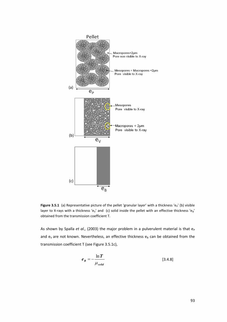
93

Figure 3.5.1 a ‘ep ese tati e pi tu e of the pellet g a ula la e ith a thi k ess eP isi le layer to X-rays ith a thi k ess eV a d solid i side the pellet ith a effe ti e thi k ess eB obtained from the transmission coefficient T.

As shown by Spalla et al., (2003) the major problem in a pulverulent material is that eP

and eV are not known. Nevertheless, an effective thickness eB can be obtained from the

transmission coefficient T (see Figure 3.5.1c),

solid

B

Te

ln

[3.4.8]

(a)

(b)

(c)

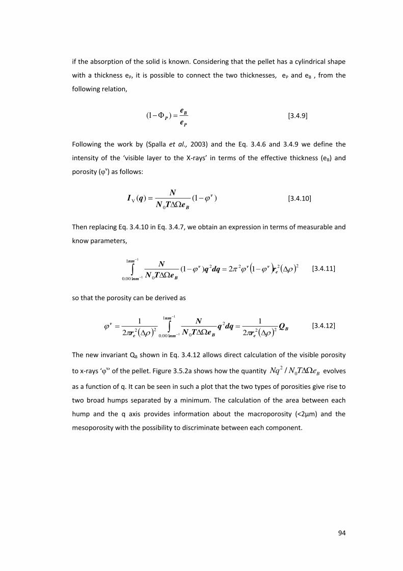
94

if the absorption of the solid is known. Considering that the pellet has a cylindrical shape

with a thickness eP, it is possible to connect the two thicknesses, eP and eB , from the

following relation,

P

BP

e

e )1( [3.4.9]

Following the work by (Spalla et al., 2003) and the Eq. 3.4.6 and 3.4.9 we define the

intensity of the isi le la e to the X-ra s in terms of the effective thickness (eB) and

porosity (φv) as follows:

)1()(0

Vv

BeTN

NqI

[3.4.10]

Then replacing Eq. 3.4.10 in Eq. 3.4.7, we obtain an expression in terms of measurable and

know parameters,

2221

001.0

2

0

12)1(1

1

e

vv

nm

nm

v

B

rdqqeTN

N [3.4.11]

so that the porosity can be derived as

B

e

nm

nm Be

v Qr

dqqeTN

N

r22

1

001.0

2

022 2

1

2

11

1

[3.4.12]

The new invariant QB shown in Eq. 3.4.12 allows direct calculation of the visible porosity

to x- a s φv of the pellet. Figu e . . a sho s ho the ua tit BeTNNq 02 / evolves

as a function of q. It can be seen in such a plot that the two types of porosities give rise to

two broad humps separated by a minimum. The calculation of the area between each

hump and the q axis provides information about the macroporosity (<2µm) and the

mesoporosity with the possibility to discriminate between each component.

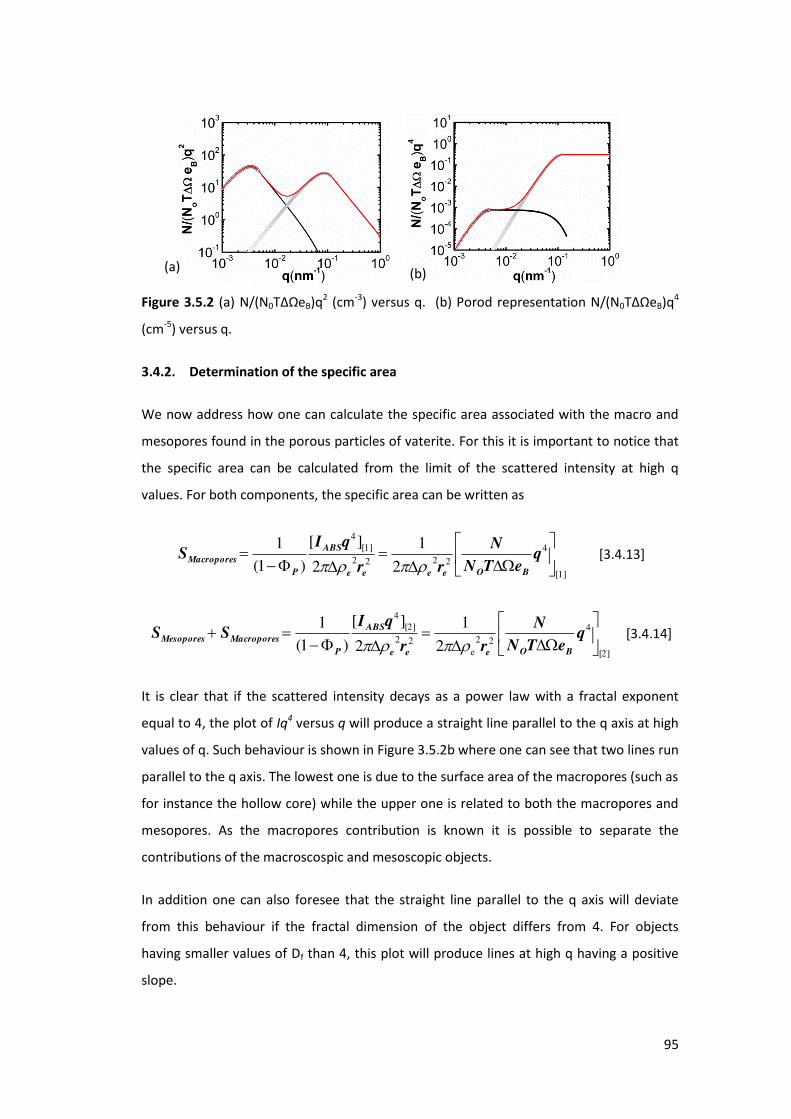
95

Figure 3.5.2 (a) N/(N0TΔΩeB)q2 (cm-3) versus q. (b) Porod representation N/(N0TΔΩeB)q4

(cm-5) versus q.

3.4.2. Determination of the specific area

We now address how one can calculate the specific area associated with the macro and

mesopores found in the porous particles of vaterite. For this it is important to notice that

the specific area can be calculated from the limit of the scattered intensity at high q

values. For both components, the specific area can be written as

[1]

42222

[1]4

2

1

2

][

)1(1

qeTN

N

rr

qIS

BOeeee

ABS

P

Macropores [3.4.13]

[2]

422

e22

[2]4

2

1

2

][

)1(1

qeTN

N

rr

qISS

BOeee

ABS

P

MacroporesMesopores [3.4.14]

It is clear that if the scattered intensity decays as a power law with a fractal exponent

equal to 4, the plot of Iq4 versus q will produce a straight line parallel to the q axis at high

values of q. Such behaviour is shown in Figure 3.5.2b where one can see that two lines run

parallel to the q axis. The lowest one is due to the surface area of the macropores (such as

for instance the hollow core) while the upper one is related to both the macropores and

mesopores. As the macropores contribution is known it is possible to separate the

contributions of the macroscospic and mesoscopic objects.

In addition one can also foresee that the straight line parallel to the q axis will deviate

from this behaviour if the fractal dimension of the object differs from 4. For objects

having smaller values of Df than 4, this plot will produce lines at high q having a positive

slope.

(b) (a)

96

3.4.3. Results and Discussions

The effective thickness eB of the sample was calculated using Eq. 3.4.8 with the

transmission coefficients (T) at 12.4 keV shown in Table 3.5.1. Taking Eq. 3.4.8 and 3.4.9

with Pe = 1.5 mm (see experimental section), the estimated total porosity is 90 and 95%

for NR and SR respectively (these values are important due to fact that pellet are not

pressed). The electron density of vaterite was calculated from the hexagonal structure of

vaterite and was found to be equal to 810 e- /nm3. The mass density of vaterite was taken

to be 2.66 g/cm3 as expected from its crystalline structure which was checked by

complementary wide angle x-ray scattering measurements. With all these information it

was possible to calculate (1) the invariant dqqeTNNQ BB

20 )/( using the TRAPZ

function in Matlab which is a built in function for numerical integration and (2) the

porosity. The interval of integration in q space was chosen to range from 10-3 nm-1 to

1nm1. Since the integration is truncated to experimental boundaries, the determination of

QB is underestimated. At low q, a correction can be applied by assuming that the intensity

is constant. At high q, the correction can be estimated by assuming that the Porod

eha iou I ≈ -Df is still valid. With such assumptions, we can estimate that QB is

reduced by about 1% at low-q, while at high-q the underestimation is about 20% of the

value corresponding to the mesopores. The results of porosity are shown in Table 3.5.1.

The porosities calculated by the Porod invariant are φv = 42% for SR and φv = 46% for the

NR. It can be seen on the plots shown in Figures 3.5.3a and 3.5.3b that the two curves are

quite similar in the low q region while they significantly differ at large q values. The

discrimination between macro and mesoporosities is possible from the fits to the data.

Each component can be calculated by replacing in QB the scattered intensity by I1(q) and

I2(q). The results for the meso and macro porosities are shown in Table 3.5.1. It can be

seen that the mesoporosity is much smaller for the supercritical route (φvMeso =12%) than

for the normal route (φvmeso=22%). Note that if we take into account the correction of QB

at high q , the mesoporosity would be for the normal route φvmeso≈ % a d fo the

supercritical route φvMeso ≈ %. O the othe ha d, the a oporosities are similar for

both samples with a somewhat higher value for the SR route φvmacro,SR=30% > φv

macro,NR

=24%. This could be the consequence of the presence of the hollow core inside the

samples prepared by the SR route or of the free space between the microspheres.

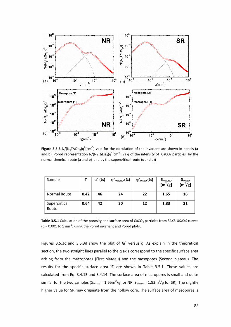
97

Figure 3.5.3 N/(N0TΔΩeB)q2[cm-3] vs q for the calculation of the invariant are shown in panels (a

and b). Porod representation N/(N0TΔΩeB)q4[cm-5] vs q of the intensity of CaCO3 particles by the

normal chemical route (a and b) and by the supercritical route (c and d))

Sample T φv (%) φvMACRO (%) φv

MESO (%) SMACRO

[m2/g] SMESO

[m2/g]

Normal Route 0.42 46 24 22 1.65 16

Supercritical Route

0.64 42 30 12 1.83 21

Table 3.5.1 Calculation of the porosity and surface area of CaCO3 particles from SAXS-USAXS curves

(q = 0.001 to 1 nm-1) using the Porod invariant and Porod plots.

Figures 3.5.3c and 3.5.3d show the plot of Iq4 versus q. As explain in the theoretical

section, the two straight lines parallel to the q axis correspond to the specific surface area

arising from the macropores (First plateau) and the mesopores (Second plateau). The

results for the specific surface area 'S' are shown in Table 3.5.1. These values are

calculated from Eq. 3.4.13 and 3.4.14. The surface area of macropores is small and quite

similar for the two samples (SMacro = 1.65m2/g for NR, SMacro = 1.83m2/g for SR). The slightly

higher value for SR may originate from the hollow core. The surface area of mesopores is

(b) (a)

(d) (c)

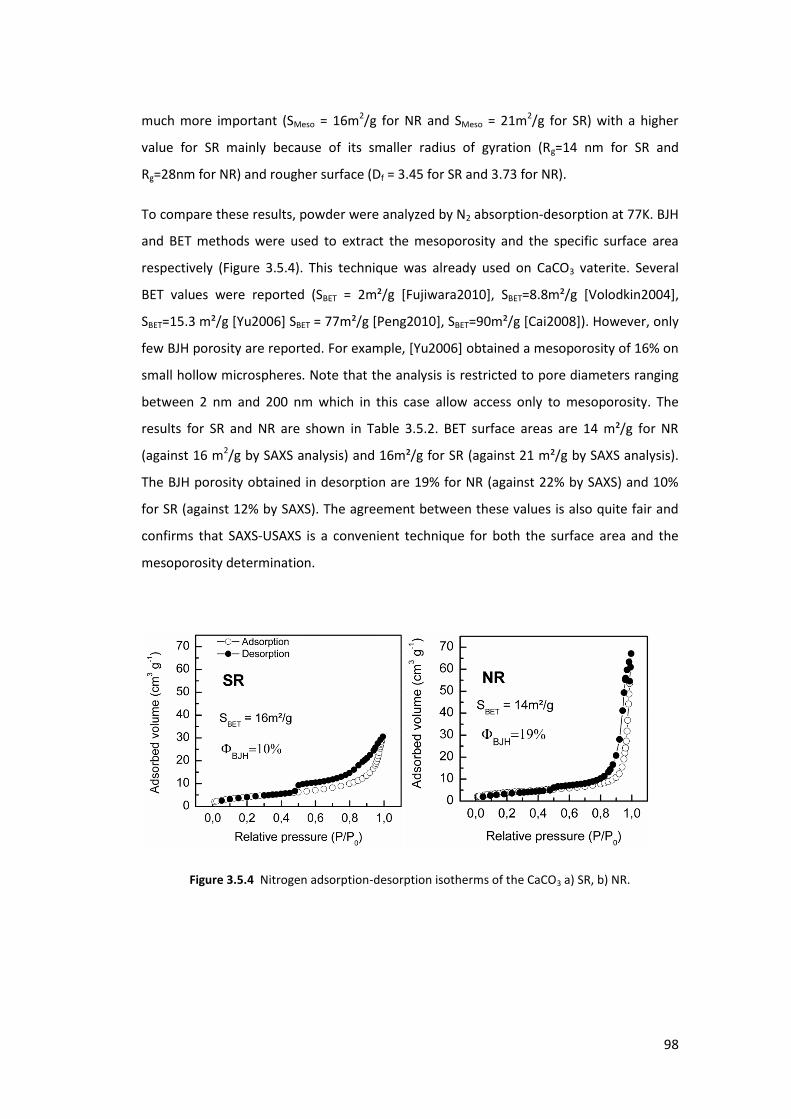
98

much more important (SMeso = 16m2/g for NR and SMeso = 21m2/g for SR) with a higher

value for SR mainly because of its smaller radius of gyration (Rg=14 nm for SR and

Rg=28nm for NR) and rougher surface (Df = 3.45 for SR and 3.73 for NR).

To compare these results, powder were analyzed by N2 absorption-desorption at 77K. BJH

and BET methods were used to extract the mesoporosity and the specific surface area

respectively (Figure 3.5.4). This technique was already used on CaCO3 vaterite. Several

BET values were reported (SBET = 2m²/g [Fujiwara2010], SBET=8.8m²/g [Volodkin2004],

SBET=15.3 m²/g [Yu2006] SBET = 77m²/g [Peng2010], SBET=90m²/g [Cai2008]). However, only

few BJH porosity are reported. For example, [Yu2006] obtained a mesoporosity of 16% on

small hollow microspheres. Note that the analysis is restricted to pore diameters ranging

between 2 nm and 200 nm which in this case allow access only to mesoporosity. The

results for SR and NR are shown in Table 3.5.2. BET surface areas are 14 m²/g for NR

(against 16 m2/g by SAXS analysis) and 16m²/g for SR (against 21 m²/g by SAXS analysis).

The BJH porosity obtained in desorption are 19% for NR (against 22% by SAXS) and 10%

for SR (against 12% by SAXS). The agreement between these values is also quite fair and

confirms that SAXS-USAXS is a convenient technique for both the surface area and the

mesoporosity determination.

Figure 3.5.4 Nitrogen adsorption-desorption isotherms of the CaCO3 a) SR, b) NR.

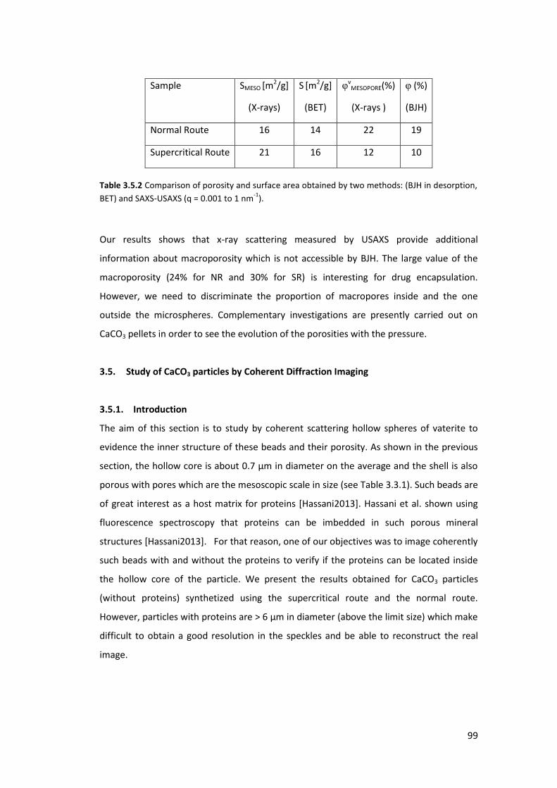
99

Sample SMESO [m2/g]

(X-rays)

S [m2/g]

(BET)

φvMESOPORE(%)

(X-rays )

φ (%)

(BJH)

Normal Route 16 14 22 19

Supercritical Route 21 16 12 10

Table 3.5.2 Comparison of porosity and surface area obtained by two methods: (BJH in desorption,

BET) and SAXS-USAXS (q = 0.001 to 1 nm-1).

Our results shows that x-ray scattering measured by USAXS provide additional

information about macroporosity which is not accessible by BJH. The large value of the

macroporosity (24% for NR and 30% for SR) is interesting for drug encapsulation.

However, we need to discriminate the proportion of macropores inside and the one

outside the microspheres. Complementary investigations are presently carried out on

CaCO3 pellets in order to see the evolution of the porosities with the pressure.

3.5. Study of CaCO3 particles by Coherent Diffraction Imaging

3.5.1. Introduction

The aim of this section is to study by coherent scattering hollow spheres of vaterite to

evidence the inner structure of these beads and their porosity. As shown in the previous

section, the hollow core is about 0.7 µm in diameter on the average and the shell is also

porous with pores which are the mesoscopic scale in size (see Table 3.3.1). Such beads are

of great interest as a host matrix for proteins [Hassani2013]. Hassani et al. shown using

fluorescence spectroscopy that proteins can be imbedded in such porous mineral

structures [Hassani2013]. For that reason, one of our objectives was to image coherently

such beads with and without the proteins to verify if the proteins can be located inside

the hollow core of the particle. We present the results obtained for CaCO3 particles

(without proteins) synthetized using the supercritical route and the normal route.

However, particles with proteins are > 6 µm in diameter (above the limit size) which make

difficult to obtain a good resolution in the speckles and be able to reconstruct the real

image.

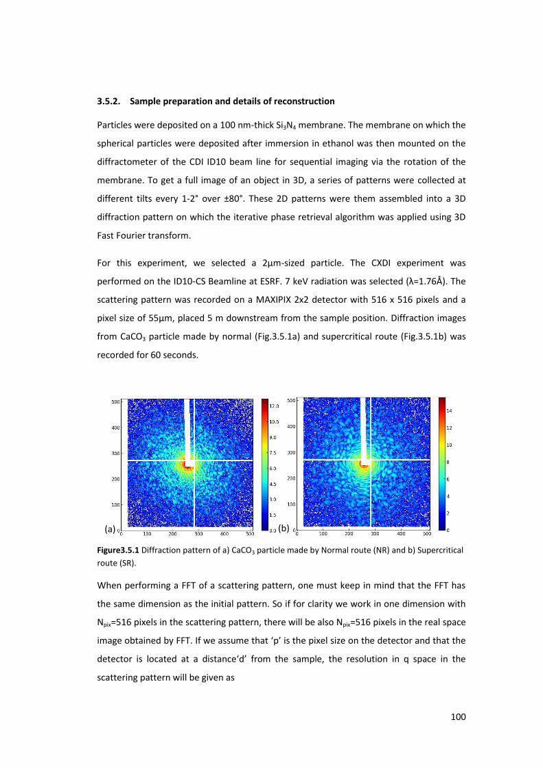
100

3.5.2. Sample preparation and details of reconstruction

Particles were deposited on a 100 nm-thick Si3N4 membrane. The membrane on which the

spherical particles were deposited after immersion in ethanol was then mounted on the

diffractometer of the CDI ID10 beam line for sequential imaging via the rotation of the

membrane. To get a full image of an object in 3D, a series of patterns were collected at

different tilts every 1-2° over ±80°. These 2D patterns were them assembled into a 3D

diffraction pattern on which the iterative phase retrieval algorithm was applied using 3D

Fast Fourier transform.

For this experiment, we selected a 2µm-sized particle. The CXDI experiment was

performed on the ID10-C“ Bea li e at E“‘F. keV adiatio as sele ted = . Å . The

scattering pattern was recorded on a MAXIPIX 2x2 detector with 516 x 516 pixels and a

pixel size of 55µm, placed 5 m downstream from the sample position. Diffraction images

from CaCO3 particle made by normal (Fig.3.5.1a) and supercritical route (Fig.3.5.1b) was

recorded for 60 seconds.

Figure3.5.1 Diffraction pattern of a) CaCO3 particle made by Normal route (NR) and b) Supercritical

route (SR).

When performing a FFT of a scattering pattern, one must keep in mind that the FFT has

the same dimension as the initial pattern. So if for clarity we work in one dimension with

Npix=516 pixels in the scattering pattern, there will be also Npix=516 pixels in the real space

i age o tai ed FFT. If e assu e that p is the pi el size o the dete to a d that the

dete to is lo ated at a dista e d f o the sa ple, the esolutio i spa e i the

scattering pattern will be given as

(a) (b)

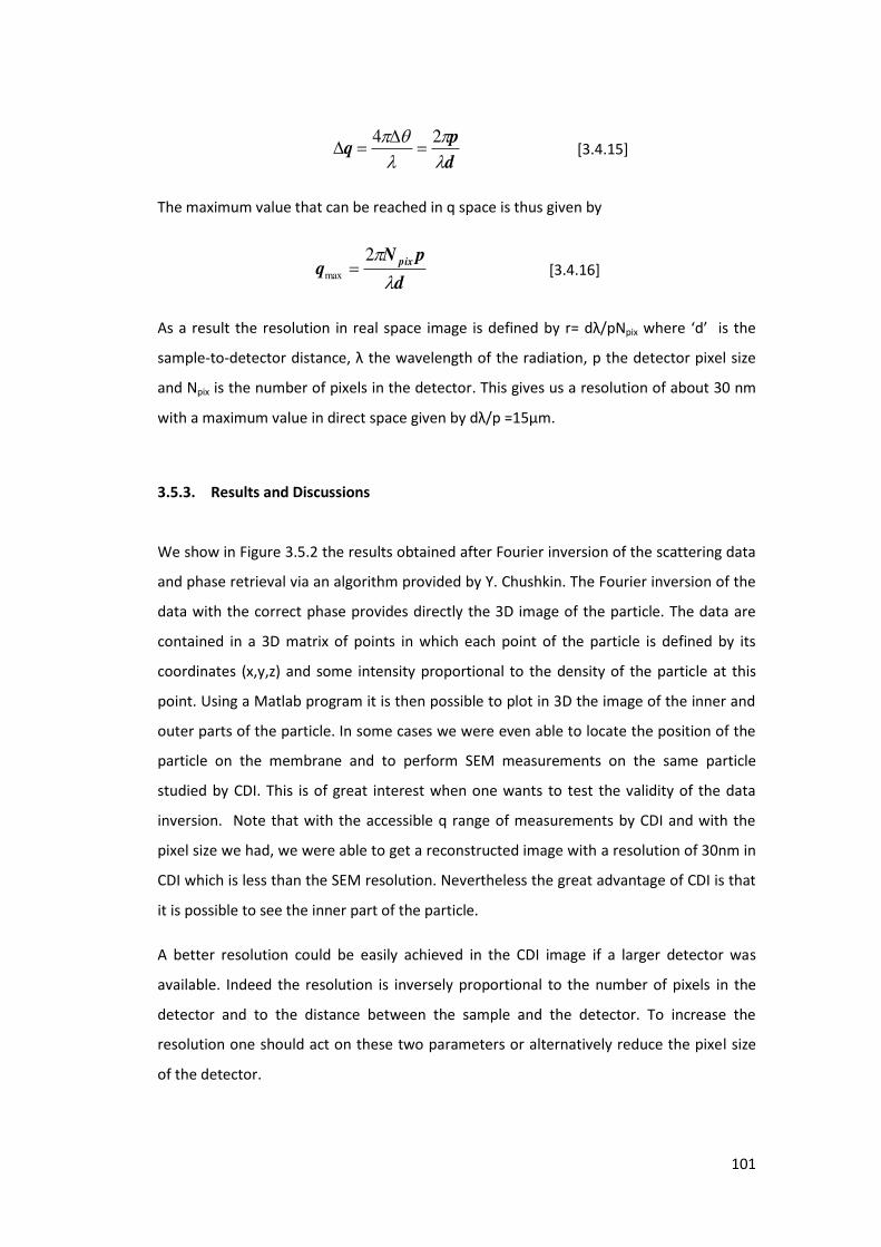
101

d

pq

24

[3.4.15]

The maximum value that can be reached in q space is thus given by

d

pNq

pix

2

max [3.4.16]

As a result the resolution in real space image is defined = d /pNpix he e d is the

sample-to-detector distance, the wavelength of the radiation, p the detector pixel size

and Npix is the number of pixels in the detector. This gives us a resolution of about 30 nm

with a maximum value in direct space given by d /p =15µm.

3.5.3. Results and Discussions

We show in Figure 3.5.2 the results obtained after Fourier inversion of the scattering data

and phase retrieval via an algorithm provided by Y. Chushkin. The Fourier inversion of the

data with the correct phase provides directly the 3D image of the particle. The data are

contained in a 3D matrix of points in which each point of the particle is defined by its

coordinates (x,y,z) and some intensity proportional to the density of the particle at this

point. Using a Matlab program it is then possible to plot in 3D the image of the inner and

outer parts of the particle. In some cases we were even able to locate the position of the

particle on the membrane and to perform SEM measurements on the same particle

studied by CDI. This is of great interest when one wants to test the validity of the data

inversion. Note that with the accessible q range of measurements by CDI and with the

pixel size we had, we were able to get a reconstructed image with a resolution of 30nm in

CDI which is less than the SEM resolution. Nevertheless the great advantage of CDI is that

it is possible to see the inner part of the particle.

A better resolution could be easily achieved in the CDI image if a larger detector was

available. Indeed the resolution is inversely proportional to the number of pixels in the

detector and to the distance between the sample and the detector. To increase the

resolution one should act on these two parameters or alternatively reduce the pixel size

of the detector.

102

Figure 3.5.2 a) SEM image b) reconstructed 3D image and c) Cross-section of CaCO3 particle made

by supercritical route (diameter = 1.9µm) d) ,e) and f) CaCO3 particles made by normal route

(diameter=3.2µm).

Figure 3.5.2 shows the comparison of the SEM picture of the sample used with the

reconstructed image. The agreement between both images is striking. The internal

structure of the particle can be observed in the cross section of the reconstructed image

(see Figure 3.5.2 c) and f)) where high and low density region confirm the porosity of the

particles.

As shown in Figures 3.5.2c) and f), the particle made by the supercritical route (SR) and by

the normal route have an average diameter of 2 . These figures show that particles

have an important mesoporosity, in addition we can observe that particles made by

supercritical route have a hollow core, while particles made by the NR do not have this

hollow core. We have to notice that CaCO3 particles (SR) analysed by USAXS and SAXS

were bigger than particles analysed by CXDI. This proves that regardless of the particle

size of CaCO3 powders made by SR these particles possess a hollow core, which is

important for applications in drug delivery.

3.6. Conclusion

We have shown in this chapter that microspheres of vaterite exhibit hierarchical porosity

made of macropores and mesopores. The quantitative determination of the pore size and

of the pore smoothness was achieved by implementing the Guinier Porod model recently

proposed by [Hammouda2010] for two types of pores. The radii of gyration of the two

components and their fractal dimension were obtained. It was found that macropores

SEM CXDI

SR

(a)

NR

(b) (c)

(d) (e) (f)

103

have fractal dimension close to 4 indicating smooth surfaces whereas mesopores located

inside the microspheres have smaller fractal dimension which highlights a rough surface.

In both cases radii of gyration are of the order of 280 nm for the macropores and about

20 times smaller for the mesopores. The porosity and the surface area was furthermore

determined following the approach of [Spalla2003] for powders by calculating a Porod

invariant based on the effective thickness of the pulverulent pellet. The specific surface

and the mesoporosity are much closed to the results extracted from the N2 adsorption-

desorption analysis. This analysis was recently complemented by CDI experiments at the

ID10A beam line of the ESRF. We were able to reconstruct in 3D the complete shape of

these particles and to evidence their inner geometry by 3D tomography.

104

105

Bibliography

[Beaucage1994] Beaucage, G.; Schaefer, D. W.. J. of Non-Cryst. Solids, (1994) 172-174,797-805.

[Beaucage2007] Sztucki, M.; Narayanan, T.; Beaucage, G., Journal of Applied Physics, (2007) 101,

114304.

[Beuvier2011] Beuvier, T.; Calvignac, B.; Delcroix, J.R.; Tram, M. K.; Kodjikian, S.; Delorme, N. ;

Bardeau, J.F.; Gibaud A. ; Boury F. J. Mater. Chem. (2011) 21, 9757-9761.

[Cho2008] Cai, A.; Xu, X.; Pan, H.; Tao, J.; Liu, R.; Tang, R.; Cho, K. J. Phys. Chem. (2008) 112,

11324–11330.

[Feigin&Svergun1987] Feigin L. A; Svergun D. I. Structure Analysis by Small-Angle X-Ray and

Neutron Scattering, edited by George W. Taylor Plenun Press. New York and London, 1987.

[Fujiwara2008] Fujiwara, M.; Shiokawa, K.; Morigaki, K.; Zhu, Y.; Nakahara, Y., Chem. Eng. J.,

(2008) 137, 14–22.

[Fujiwara2010] Fujiwara, M.; Shiokawa, K.; Araki, M.; Ashitaka, N.; Morigaki, K.; Kubota, T.;

Nakahara Y. Crystal Growth Design (2010) 10 (9), 4030-4037.

[Gibaud1996] Gibaud, A.; Xue J.S.; Dahn, J. R. Carbon, (1996) 34, 499.

[Glatter&Kratiky1982] Glatter,O.; Kratiky, O. Small Angle x-ray scattering, Academic Press London,

1982.

[Guinier&Fournet1955] Guinier, A. ; Fournet, G. Small Angle sacttering of x-rays, Wiley, 1955.

[Kalliat1981] Kalliat, M.; Kwak, C. Y.; Schmidt P. W. i Ne App oa hes i Coal Che ist B. D.

Blaustein; B. C. Bockrath,; S. Friedman, Eds.), (1981). Am.Chem. Soc. Symp. Ser. 169, p.3. Am.

Chem. Soc., Washington, DC.

[Hammouda2010] Hammouda, B. J. Appl. Cryst. (2010) 43, 716-719.

[Hassani2013] Hassani, L.; Hindré, F.; Beuvier, T.; Calvignac, B.; Lautram, N.; Gibaud, A.; Boury, F.,

J. Mater. Chem. B, (2013) 1, 4011.

[He2009] He, X. W.; Liu, T.; Xiao, Y.; Feng, Y. L.; Cheng, D. J.; Tingting, G.; Zhang, L.; Zhang, Y.;

Chen, Y. X., Cancer Biother.Radiopharm. (2009) 24, 249–259.

[Ikoma2007] Ikoma, T.; Tonegawa, T., Watanaba, H.; Chen, G.; Tanaka J.; Mizushima, Y.; J. Nanosci.

Nanotechnol., (2007) 7, 822–827.

[Lucas-Girot2005] Lucas-Girot, A.; Verdier, M.C.; Tribut, O.; Sangleboeuf, J. C.; Allain; H.;

Oudadesse, H., J. Biomed. Mater. Res., Part B, (2005) 73, 164–170.

[Peng2010] Peng, C.; Zhao, Q.; Gao, C. Colloids Surf. A, (2010) 353, 132– 139.

[Radlinski2004] Radlinski, A.P.; Mastalerz, M.; Hinde, A.L.; Hainbuchner, M.; Rauch, H.; Baron, M.;

Lin, J.S.; Fan, L. ; Thiyagarajan, P., International Journal of Coal Geology. (2004) 59, 245– 271.

[Schmidt1982] Schmidt, P.W. J. Appl. Cryst. (1982), 15, 567–569.

[Spalla2003] Spalla, O.; Lyonnard, S.; Testard, F. J. Appl. Cryst. (2003) 36, 338-347.

[Temmerman2011] De Temmerman, M.L. ; Demeester, J. ; De Vos, F. ; De Smedt S. C.,

Biomacromolecules (2011) 12, 1283–1289.

106

[Volodkin2004] Volodkin, D.; Larionova, N. I.; Sukhorukov, G. B.; Biomacromolecules, (2004) 5,

1962-1972.

[Wie 2008] Wei, W.; Ma, G.H.; Hu, G.; Yu, D.; Mcleish, T.; Su, Z.G.; Shen, Z.Y. J. Am. Chem. Soc.

(2008) 130, 15808–15810.

[Yu2006] Yu, J.; Guo, H.; Davis, S. A.; Mann, S. Adv. Funct. Mater. (2006) 16, 2035–2041.

[Zhao2010] Zhao, Y.; Lu, Y.; Hu, Y.; Li, J.P.; Dong, L.; Lin, L.N.; Yu, S.H.; Small, (2010) 6, 2436–2442.

[Zhao2012] Zhao, D.; Zhuo, R.X.; Cheng, S.X. Mol. BioSyst. (2012) 8, 753–759.

107

CHAPTER 4

4. Study of Polystyrene Ultra thin films exposed to

supercritical CO2

This chapter is mainly devoted to the study of polystyrene ultra thin films exposed to CO2

under pressure. Before discussing the effect of pressure, it is important to highlight that

PS may dewet the HF-treated surface of a silicon substrate depending on the thickness of

the film which is initially formed. For very thin films, one can observe that films dewet the

surface yielding the formation of islands with a given shape and a certain degree of

correlation. After some generalities about polystyrene which is the polymer used in this

study, the first part of this chapter will be devoted to a discussion concerning the reasons

for which a thin film may dewet the surface of silicon in the framework of the effective

interfacial potential. In the remaining part, we study the influence of CO2 pressure on

homogeneous films and islands focusing mainly on the swelling of PS and on the effect of

pressure on the islands stability.

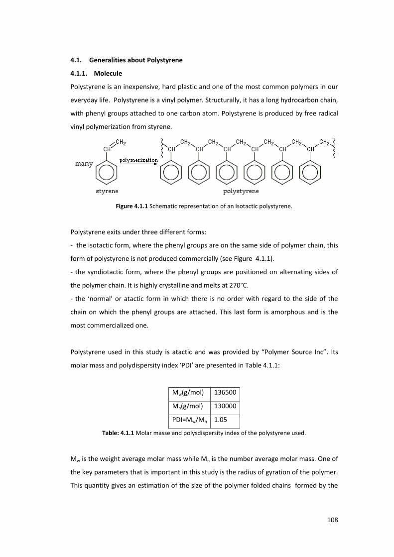
108

4.1. Generalities about Polystyrene

4.1.1. Molecule

Polystyrene is an inexpensive, hard plastic and one of the most common polymers in our

everyday life. Polystyrene is a vinyl polymer. Structurally, it has a long hydrocarbon chain,

with phenyl groups attached to one carbon atom. Polystyrene is produced by free radical

vinyl polymerization from styrene.

Figure 4.1.1 Schematic representation of an isotactic polystyrene.

Polystyrene exits under three different forms:

- the isotactic form, where the phenyl groups are on the same side of polymer chain, this

form of polystyrene is not produced commercially (see Figure 4.1.1).

- the syndiotactic form, where the phenyl groups are positioned on alternating sides of

the polymer chain. It is highly crystalline and melts at 270°C.

- the o al o ata ti form in which there is no order with regard to the side of the

chain on which the phenyl groups are attached. This last form is amorphous and is the

most commercialized one.

Pol st e e used i this stud is ata ti a d as p o ided Pol e “ou e I . Its

ola ass a d pol dispe sit i de PDI a e p ese ted i Ta le . . :

Mw(g/mol) 136500

Mn(g/mol) 130000

PDI=Mw/Mn 1.05

Table: 4.1.1 Molar masse and polysdispersity index of the polystyrene used.

Mw is the weight average molar mass while Mn is the number average molar mass. One of

the key parameters that is important in this study is the radius of gyration of the polymer.

This quantity gives an estimation of the size of the polymer folded chains formed by the

109

polymer. It is defined by the root mean square distance from the centre of mass to any

points in the polymer coil. For atactic polystyrene, the unperturbed radius of gyration is

given by RG=0.0272 MW1/2 where MW is expressed in g/mol and RG in nm. With the

polystyrene used in this study, we obtain RG ≈ .04nm [Israelachvili2011].

4.1.2. Glass Transition and Free volume

In polymers, the glass transition describes the change from a glassy state to a rubbery

state. This change is defined by the glass transition temperature Tg. Despite a huge

amount of studies devoted to the characterization of the physical properties through the

glass transition of polymers samples both in bulk and in thin films, a detailed

understanding of the glass transition in thin films is still a matter of continuous debate

and research. For a discussion of the relevant issues, the reader can refer to the papers of

[Donth2001, Angell2000].

Of particular interest to describe the glass transition and in a more general point of view

to explain the evolution of physical properties with temperature are the concepts of chain

mobility and free volume [Cohen1959].

When a polymer is in the liquid or rubbery state, the amount of free volume increases

with temperature as a result of easier molecular motion. When temperature is decreased,

the free volume contracts and eventually reaches a critical value where there is

insufficient free space to allow large scale segmental motion to take place. The

temperature for which this critical volume is reached is the glass transition temperature.

Below Tg the free volume remains essentially constant as the temperature decreases

further, since the chains are immobilized and frozen in position [Cohen1959, Dinelli2000].

The free volume of polymers is generally defined by Vf = V - Vocc where V is the total and

Vocc the occupied volume. The occupied volume corresponds to the van der Waals volume.

This volume is dictated by the size of the atoms and their covalent bonds and is also

independent of the conformation of the polymer. The free volume is defined as the

difference between the specific and occupied volumes. It can be defined as the small

amount of unfilled volume. Recent investigations using positron annihilation reveals that

the diameter of these holes is approximately 0.5 nm [Ata2009]. The free volume is

associated with inter chains and end chains free volumes. The later is represented in the

diagram below).

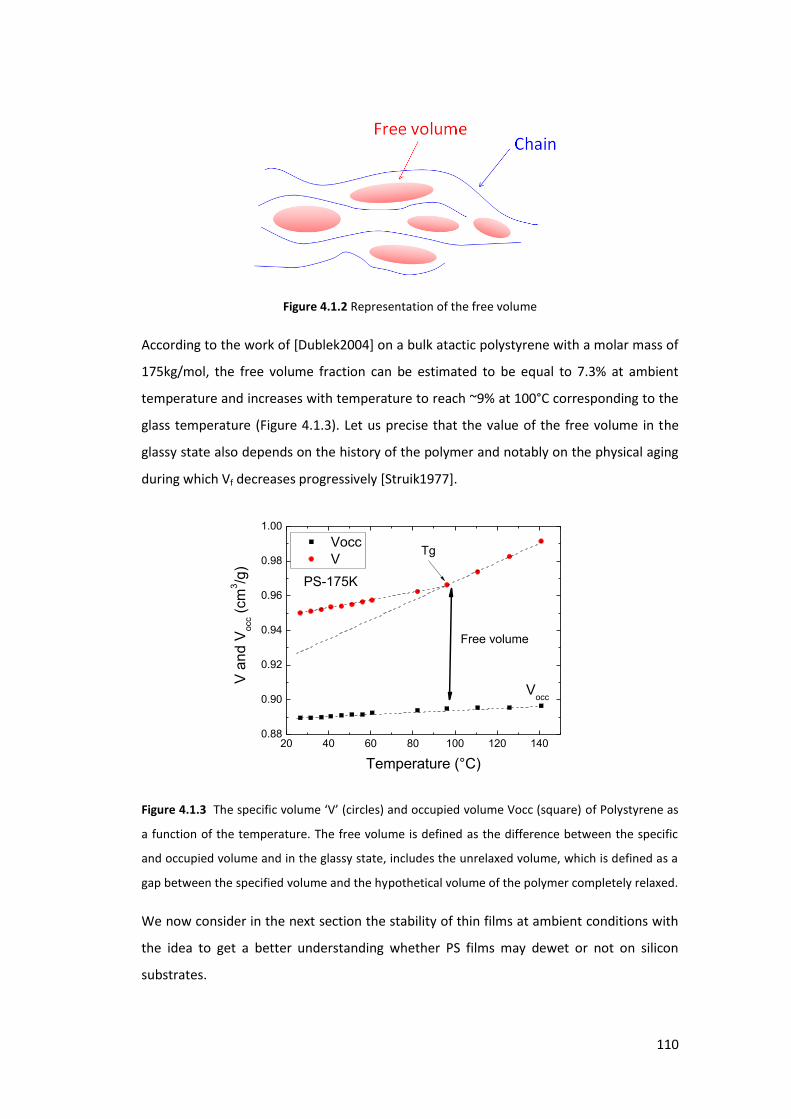
110

Figure 4.1.2 Representation of the free volume

According to the work of [Dublek2004] on a bulk atactic polystyrene with a molar mass of

175kg/mol, the free volume fraction can be estimated to be equal to 7.3% at ambient

temperature and increases with temperature to reach ~9% at 100°C corresponding to the

glass temperature (Figure 4.1.3). Let us precise that the value of the free volume in the

glassy state also depends on the history of the polymer and notably on the physical aging

during which Vf decreases progressively [Struik1977].

20 40 60 80 100 120 1400.88

0.90

0.92

0.94

0.96

0.98

1.00

Vocc

V

V a

nd

Vocc (

cm

3/g

)

Temperature (°C)

Free volume

Vocc

PS-175K

Tg

Figure 4.1.3 The spe ifi olu e V i les a d o upied olu e Vo s ua e of Polystyrene as

a function of the temperature. The free volume is defined as the difference between the specific

and occupied volume and in the glassy state, includes the unrelaxed volume, which is defined as a

gap between the specified volume and the hypothetical volume of the polymer completely relaxed.

We now consider in the next section the stability of thin films at ambient conditions with

the idea to get a better understanding whether PS films may dewet or not on silicon

substrates.

111

4.1.3. Stability of thin films and the dewetting process

4.1.3.1. Spreading coefficient

The dewetting process is one of the most remarquable phenomena that can occur at a

solid–liquid or liquid–liquid interface. In general, dewetting describes the rupture of a thin

liquid film on a substrate and the subsequent formation of droplets. A very simple

example of this phenomenon is the formation of drops at the surface of leafs after

raining. The opposite process is called spreading. Dewetting and spreading are

fundamental processes in the daily life with numerous applications for instance in

painting, hydrophobic coatings, oil recovery [Bertrand2002], efficient deposition of

pesticides on plant leaves [Bergeron2000], but also in the drainage of water from

highways [Shahidzadeh2003] and the cooling of industrial reactors. On a smaller scale,

wetting solutions have been proposed to solve technological problems in microfluidics

and nanoprinting, inkjet printing etc. [Tabeling2004]. As underlined by Bonn et al. wetting

phenomena are a playground where chemistry, physics and engineering intersect

[Bonn2009]. From a macroscopic point of view, the spontaneous spreading or dewetting

for a drop placed on a solid substrate is governed by the so-called spreading coefficient S.

This parameter is defined as the difference between the energy of the dry substrate and

the energy of the same substrate wetted by the liquid.

WETDRY EES [4.1.3]

Figure 4.1.4 Two situations of spreading coefficients: S>0, total wetting situation, the liquid

spreads spontaneously on the substrate and form a film. S<0 the liquid does not spread

spontaneously, the triple line form an angle with the substrate.

Considering E as the energy per unit area we can write :

SLSGS [4.1.4]

112

with SG ,

SL and the solid-gas, solid-liquid and liquid-gas interfacial tensions,

respectively. EDRY corresponds to SG . EWET corresponds to

SL + . The parameter S is

used to evaluate qualitatively the behavior of the liquid on the substrate.

If S is negative, the situation where the solid is covered by a liquid film is not favorable.

The equilibrium shape of a drop that is smaller than the capillary length is a spherical cap,

characterized by its equili iu o ta t a gle θ see Fig. . . , defi ed the You g-

Dup s e uatio . If “ is positi e, the li uid sp eads a d te ds to o e the a i u

surface area.

SG (mJ/m2)

(Si with native oxide)

36.5 Zhao1993

SG (mJ/m2)

(Si treated with HF)

44.7

Zhao1993

(mJ/m2) (PS) 38.7 36

Wu1982 Lee1968

Table 4.1.2 List of interfacial tensions.

4.1.3.2. Stability and excess free energy of a thin film

The stability of a polymer thin film with respect to dewetting is related to its thickness. As

expected from the definition of the spreading coefficient, thick film (h> 100nm) are stable

when S is positive. However, for thinner film (h< 100 nm), excess intermolecular

interaction free energy can be dominant and spontaneous dewetting can occur even

though the spreading coefficient S is positive.

The stability of a system depending on a single parameter such as the thickness h can be

apprehended by using the conceptual model of free energy. The free energy of a system

based on its potential energy is the key physical quantity that describes the stability of a

system. In many areas of physics, this concept is of fundamental importance because it

allows to predicting the stability of a system independently of the time variable as for

instance in astronomy for the observation of periodic comets or in condensed matter

physics to understand the behavior of phase transitions via the order parameter. One of

the major problems to address with thin films is to properly determine the free energy of

113

the system. This is not a simple question and many authors have tried to explain how to

describe it without being able to give its exact analytical expression. The work of F.

Brochard-Wyart et al. is of great interest to understand in a conceptual way how a thin

film behaves when it is cast on a substrate [Brochard-Wyart1990]. For this reason we are

going to first present some of the key points introduced in this paper keeping in mind that

other models have also been proposed by other authors [Mukherjee2011, Seeman2001].

In the model of Brochard-Wyart , the free energy G(h) is written as a function of the film

thickness as :

)()( hGhG SL [4.1.5]

I this e p essio ΔG is the e ess f ee e e g that is dete i ed the diffe e e

between the cohesive interactions holding the liquid together, and the adhesive

interactions between the liquid and the solid. Thus, the excess free energy has to be

given by a combination of short-range (repulsive) and long-range (attractive) interactions.

In the model of Brochard-Wyart et al. the short range interactions are related to

sp eadi g oeffi ie t “ th ough , ΔG h→ =“ a d the lo g a ge i te a tio s a e given by

the van der Waals i te a tio , ΔG h = -A/ h2, where A is the Hamaker constant (Note

that the sign of A is not defined like this in the original paper). From these relations, we

can o se e that ΔG h is go e ed t o pa a ete s: the sig of the Hamaker constant

A a d the sig of “. It is o th oti g that the t ue e p essio of ΔG h a ot e this o e

si e he h→ , the Va de Waals i te a tio is ot ph si all defi ed a d ust e

corrected by a repulsive term that precludes the penetration of molecules.

Since for a thin film on a substrate, A and S may have any sign, four different cases are to

be distinguished. For instance when S >0 and A>0 which is the model mostly used in our

calculations, a final equilibrium state is a wetting film of thickness heq and a residual

droplet over the wetting film. (see Fig. 4.1.5 c) and d) ). This kind of situation is very

interesting since it is contrary to the common belief that the formation of droplets is only

valid for S<0. Hence for thin films (h<100nm) the sign of the Hamaker constant has also to

be specified to evaluate the stability of the system.

114

COMPLETE WETTING A<0 and S>0

PARTIAL WETTING A>0 and S<0

PEUDO PARTIAL WETTING A>0 and S>0

Figure 4.1.5 a), c) and e) Free energy corresponding to A<0, S>0 , A>0, S<0 and A>0, S>0 and its

associated b),d) and f) final equilibrium state of a film showing a droplet and a wetting layer of

thickness heq.

The main drawback of Brochard Wyart et al.'s model is that it does not provide the full

analytical expression for the potential. To circumvent such a drawback a few authors have

proposed to include in the potential a repulsive term that is generally not very well

justified. For instance, Seemann et al. proposes an analytic expression for the free energy

in which the , van der Walls potential as usually defined by [Semann2001] :

212)(

h

AhVDW

[4.1.6]

is modified by a repulsive term that characterizes short-range interactions of strength c

as:

)()(8

hh

ch VDW [4.1.7]

(a) (b)

(c) (d)

(e) (f)

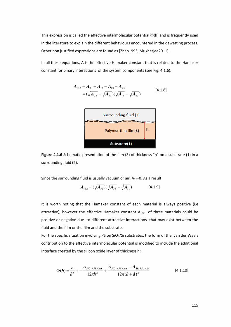
115

This expression is called the effective intermolecular potential Ф(h) and is frequently used

in the literature to explain the different behaviours encountered in the dewetting process.

Other non justified expressions are found as [Zhao1993, Mukherjee2011].

In all these equations, A is the effective Hamaker constant that is related to the Hamaker

constant for binary interactions of the system components (see Fig. 4.1.6).

))(( 33113322

23131233132

AAAA

AAAAA

[4.1.8]

Figure 4.1.6 Schematic presentation of the film of thi k ess h o a su st ate i a

surrounding fluid (2).

Since the surrounding fluid is usually vacuum or air, A22=0. As a result

))(( 113333132 AAAA [4.1.9]

It is worth noting that the Hamaker constant of each material is always positive (i.e

attractive), however the effective Hamaker constant A132 of three materials could be

positive or negative due to different attractive interactions that may exist between the

fluid and the film or the film and the substrate.

For the specific situation involving PS on SiO2/Si substrates, the form of the van der Waals

contribution to the effective intermolecular potential is modified to include the additional

interface created by the silicon oxide layer of thickness h:

2

////

2

//

8 )(1212)( 22

dh

AA

h

A

h

ch

AirPSSiAirPSSiOAirPSSiO

[4.1.10]

116

where d is the silicon oxide thickness, ASiO2/PS/Ai is the Hamaker constant of the

SiO2/PS/Air and ASi/PS/Air is the Hamaker constant of the Si/PS/Air.

Seemann et al. assesses the stability of the film by the second derivative of the potential

Ф h . If Ф h < the fil ill de et spo ta eousl , ut if Ф h > , the fil ill e

stable. As an illustration, qualitative variations of Ф(h) and Ф h are shown in Figure

4.1.7 using a realistic set of parameters. Figure 4.1.7a shows a scenario where Ф(h)> 0. In

this case, the film is stable. In Figure 4.1.7b there is a global minimum Ф(h) at h=heq. Here

the system can gain energy by changing its thickness to h0=heq. If the initial thickness is

larger than heq, the film will dewet and the film will be unstable. Finally, in Figure 4.1.7c

the film is unstable for Ф h < a d sta le fo Ф h > .

3 6 9

-0.06

0.00

0.06

(h

) m

J/m

2

film thickness (nm)

''>0

2 4 6 8

-0.04

0.00

0.04

(h

) m

J/m

2

film thickness (nm)h

eq

''<0

2 4 6

-0.03

0.00

0.03 ''<0

(h

) m

J/m

2

film thickness(nm)h

eq

''>0

Figure 4.1.7 Sketches of the effective interface potential φ h solid li e a d φ h dashed li e for (a) a stable (b)an unstable and (c)a metastable system. The parameters used for the

simulations of these curves are: for (a) system Si/PS/Air, ASi/PS/Air =–5.9×10-20J, (b) system

Si/SiO2/PS/Air (hSiO2=190nm) ASi/PS/Air = –5.9×10-20J, ASiO2/PS/Air = 2.2x10-20J , c= 6.3x10-76Jm6, for (c)

system Si/SiO2/PS/Air (hSiO2=1nm), ASi/PS/Air = -5.9×10-20J, ASiO2/PS/Air = 2.2x10-20J , c=0.09x10-76Jm6

The position of the minimum defines the equilibrium film thickness heq due to the fact

that a stable residual film of this thickness remains after dewetting, also called the

wetting layer or residual layer. This has been experimentally verified by X-ray scattering

measurements for short-chained polystyrene films (heq = 1.3 nm for a molecular weight

Mw =2.05 kg mol-1, te ed P“ k o a “i afe ith a “iO2 layer

[Seemann2001].

(a) (b) (c)

117

4.1.3.3. Theoretical and Experimental expressions of the Hamaker constant

The non retarded Hamaker constant A123 for medium 2 between medium 1 and 3 is given

from Lifshitz theory [Israelachvili2011] by

])()[()()(

))((

28

3h

4

3

2/123

22

2/123

21

2/123

22

2/123

21

23

22

23

21e

32

32

31

31

00123

nnnnnnnn

nnnn

kT

AAA

[4.1.11]

he e i is the dielectric constant of medium i in the zero frequency limit, ni the index of

refraction in the isi le f e ue , υe the electronic absorption frequency, h is the Planck

constant, K is the Boltzmann constant and T is the temperature . A t pi al alue fo υe is

≈ 15 Hz. In the symmetrical case where medium 3 and 1 are the same, eq. 4.1.11

reduces to

2/322

21

222

21

2

21

21121

)(

28

343

nn

nnhkTA e

[4.1.12]

APS/PS x10-20 (J)

6.15 - 6.60

6.5 ~10.7

Hough1980 Calculated using eq. [4.1.12]* PS thin film [Li2007]**

ASi/Si x10-20 (J) 22.1 - 25.6 18

Visser1972 Calculated using eq. [4.1.12]***

ASiO2/SiO2 x10-20 (J) 6.4 - 6.6 6.3

Hough1980, Bergstrom1997 Calculated using eq. [4.1.12]****

ASi/PS/Air (J) -6.2 x 10-20

-5.9x10-20 -13 x 10-20

Calculated using eq. [4.1.9] and ASi/Si=25.6 x10-20(J) and APS/PS=6.3 x10-20(J) Calculated using eq. [4.1.9] and ASi/Si=25.6 x10-20(J) and APS/PS=10.7 x10-20(J) for thin film Seemann 2001 (exp.)

ASiO2/PS/Air (J) 2.2 x 10-20 Seeman2001 (exp.) * = . , = . , υe=2.3x10-15 s-1 for Polystyrene bulk * * = . , = . , υe=2.3x10-15 s-1 for Polystyrene thin film [Ata2012] *** = . , = . , υe=0.80x10-15 s-1 for Silicon[Israelachvili2011] **** = . , = . , υe=3.2x10-15 s-1 for SiO2 [Israelachvili2011]

Table 4.1.3 List of Hamaker constant calculated and reported in the literature.

118

The first term in the eq. 4.1.12 gives the zero frequency contribution to the Van der Waals

interaction. The second term is the contribution from the dispersion energy. It is only an

approximation containing the first term of an infinite series. Since hυe>> kT, the dispersive

part usually dominates unless the refractive index of two involved materials e are similar.

The zero-frequency contribution therefore only accounts for few percents of the total

magnitude of the Hamaker constant since it cannot excess the value of 3/4kBT = 10-21J.

The next table gives the Hamaker constants of PS, SiO2, Si, Si/PS/Air, SiO2/PS/Air

calculated using the eq. [4.1.9] and [4.1.12]. Experimentally determined values are also

included.

4.1.3.4. Dewetting Mechanism

In the following is discussed the two most important mechanisms occurring in the

dewetting process of thin polymer films on a solid substrate. These two are called the

spinodal dewetting and the nucleation of holes [Xie1998, Seemann2000].

- Spinodal Dewetting

Spinodal dewetting is an intrinsic mechanism leading to the rupture of a film. It involves

an amplification of the capillary waves induced by thermal fluctuations, due to VdW

instability. This dewetting generally occurs for very thin films (<10nm). For this

mechanism, the te spi odal de etti g has ee oi ed i a alog to the phase

separation involved in a composition and decomposition process. In this process, the

height fluctuations in dewetting correspond to the composition fluctuations in phase

separation. The spatial-temporal fluctuation of the film thickness was given by [Xie1998]:

xi

hhtxZ2

exp),( 0 , )exp(0 Rthh [4.1.13]

where h0 is the film thickness, is the amplitude fluctuation and R is the growth rate.

The x-coordinate is taken to e pa allel to the su fa e a d de ote the ha a te isti

wave length. Eventually the roughening leads to rupturing of the initially smooth and

119

continuous films, at the point where the undulations grow sufficiently to expose the

underlying substrate.

Figure 4.1.8 Schematic figure illustrating a liquid film of initial height ho that undergoes a surface

height fluctuations due to capillary waves. These fluctuations in the film thickness are amplified

and lead to spontaneous dewetting of the liquid (spinodal dewetting).

- Nucleation Dewetting

Another way for a film to break up is the nucleation and growth of holes. The nucleation

mechanism considers the dewetting phenomena induced either by defects

(contamination, etc) in polymer film, by defects on the solid surface or by thermal

fluctuations of the polymer surface. The presence of particles or impurities can lower the

energy barrier leading to film thinning and holes appearing in the film at the sites of

particles (which are normally randomly distributed) [Jacobs1998].

Figure 4.1.9 Two major rupture mechanisms of thin film are: Spinoidal dewetting and the

nucleation of holes. Pictures taken from [Tsui2003]

4.2. Preparation of Polystyrene Ultra thin film and Stability

In this section, the procedure used to prepare PS thin films is described. In addition the

stability of polystyrene thin films at ambient conditions is studied by AFM and GISAXS.

Spinoidal dewetting Nucleation of holes

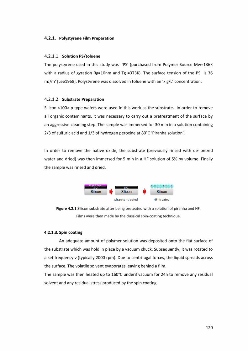
120

4.2.1. Polystyrene Film Preparation

4.2.1.1. Solution PS/toluene

The pol st e e used i this stud as P“ pu hased f o Pol e “ou e M = K

with a radius of gyration Rg=10nm and Tg =373K). The surface tension of the PS is 36

mJ/m2 [Lee ]. Pol st e e as dissol ed i tolue e ith a g/L o e t ation.

4.2.1.2. Substrate Preparation

Silicon <100> p-type wafers were used in this work as the substrate. In order to remove

all organic contaminants, it was necessary to carry out a pretreatment of the surface by

an aggressive cleaning step. The sample was immersed for 30 min in a solution containing

/ of sulfu i a id a d / of h d oge pe o ide at °C Pi a ha solutio .

In order to remove the native oxide, the substrate (previously rinsed with de-ionized

water and dried) was then immersed for 5 min in a HF solution of 5% by volume. Finally

the sample was rinsed and dried.

Figure 4.2.1 Silicon substrate after being preteated with a solution of piranha and HF.

Films were then made by the classical spin-coating technique.

4.2.1.3. Spin coating

An adequate amount of polymer solution was deposited onto the flat surface of

the substrate which was hold in place by a vacuum chuck. Subsequently, it was rotated to

a set f e ue t pi all p . Due to e t ifugal fo es, the li uid sp eads a oss

the surface. The volatile solvent evaporates leaving behind a film.

The sample was then heated up to 160°C under3 vacuum for 24h to remove any residual

solvent and any residual stress produced by the spin coating.

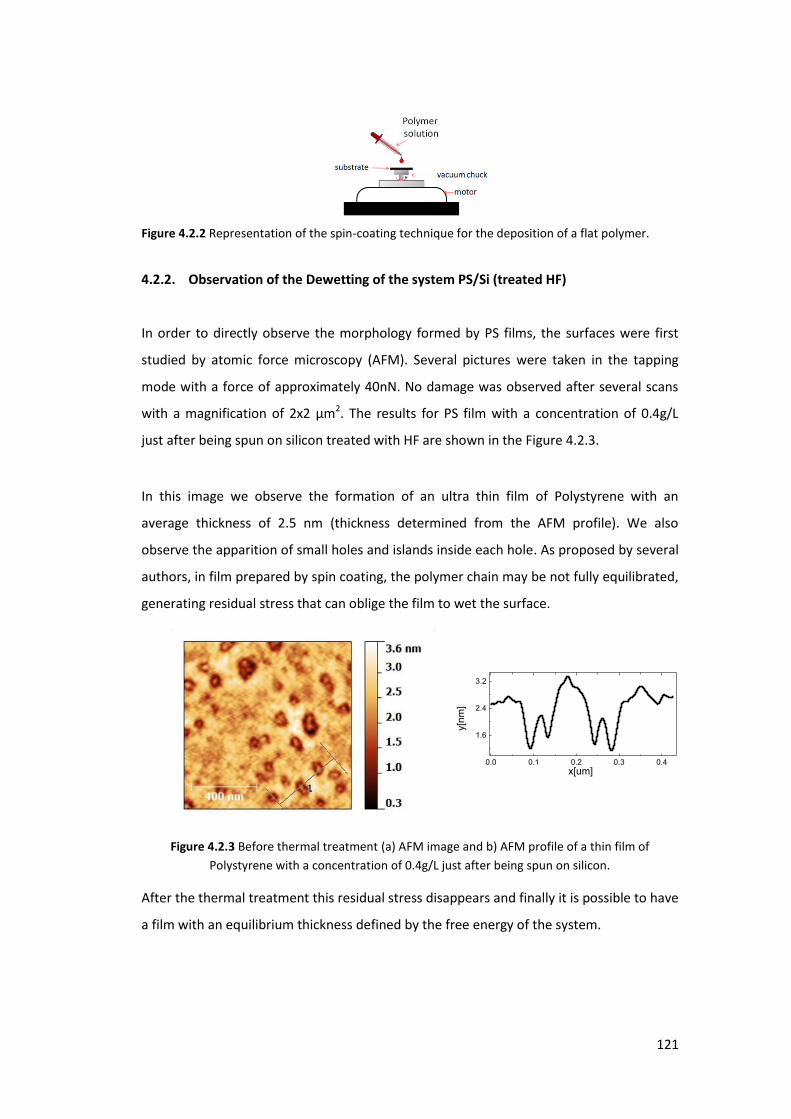
121

Figure 4.2.2 Representation of the spin-coating technique for the deposition of a flat polymer.

4.2.2. Observation of the Dewetting of the system PS/Si (treated HF)

In order to directly observe the morphology formed by PS films, the surfaces were first

studied by atomic force microscopy (AFM). Several pictures were taken in the tapping

mode with a force of approximately 40nN. No damage was observed after several scans

with a magnification of 2x2 µm2. The results for PS film with a concentration of 0.4g/L

just after being spun on silicon treated with HF are shown in the Figure 4.2.3.

In this image we observe the formation of an ultra thin film of Polystyrene with an

average thickness of 2.5 nm (thickness determined from the AFM profile). We also

observe the apparition of small holes and islands inside each hole. As proposed by several

authors, in film prepared by spin coating, the polymer chain may be not fully equilibrated,

generating residual stress that can oblige the film to wet the surface.

Figure 4.2.3 Before thermal treatment (a) AFM image and b) AFM profile of a thin film of

Polystyrene with a concentration of 0.4g/L just after being spun on silicon.

After the thermal treatment this residual stress disappears and finally it is possible to have

a film with an equilibrium thickness defined by the free energy of the system.

0.0 0.1 0.2 0.3 0.4

1.6

2.4

3.2

y[n

m]

x[um]

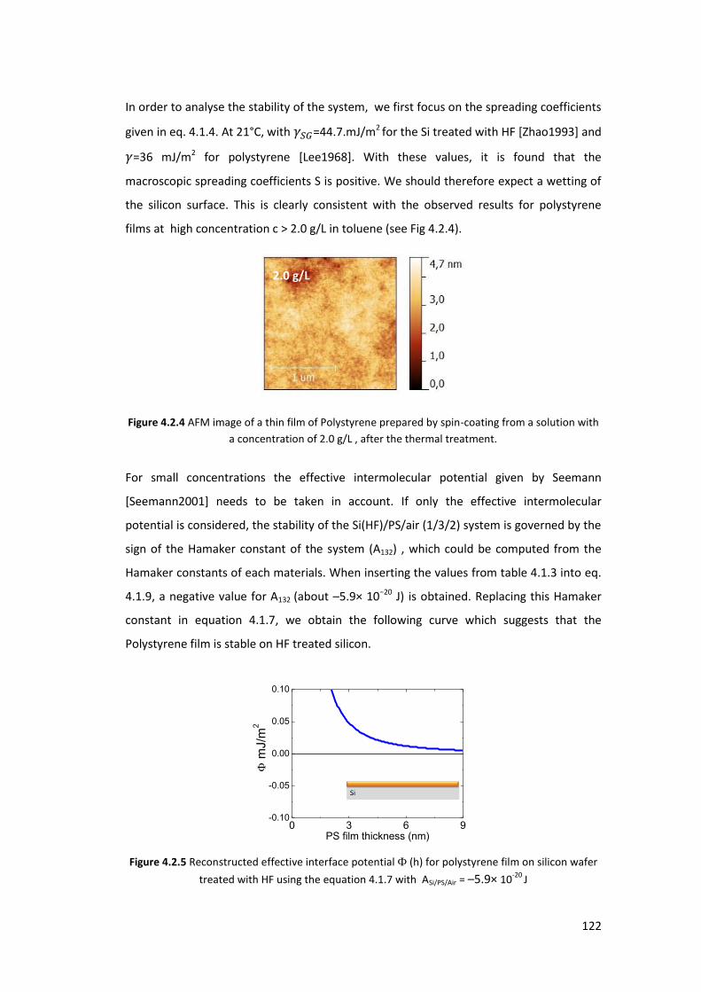
122

In order to analyse the stability of the system, we first focus on the spreading coefficients

given in eq. 4.1.4. At 21°C, with =44.7.mJ/m2 for the Si treated with HF [Zhao1993] and =36 mJ/m2 for polystyrene [Lee1968]. With these values, it is found that the

macroscopic spreading coefficients S is positive. We should therefore expect a wetting of

the silicon surface. This is clearly consistent with the observed results for polystyrene

films at high concentration c > 2.0 g/L in toluene (see Fig 4.2.4).

Figure 4.2.4 AFM image of a thin film of Polystyrene prepared by spin-coating from a solution with

a concentration of 2.0 g/L , after the thermal treatment.

For small concentrations the effective intermolecular potential given by Seemann

[Seemann2001] needs to be taken in account. If only the effective intermolecular

potential is considered, the stability of the Si(HF)/PS/air (1/3/2) system is governed by the

sign of the Hamaker constant of the system (A132) , which could be computed from the

Hamaker constants of each materials. When inserting the values from table 4.1.3 into eq.

4.1.9, a negative value for A132 (about –5.9× 10− J) is obtained. Replacing this Hamaker

constant in equation 4.1.7, we obtain the following curve which suggests that the

Polystyrene film is stable on HF treated silicon.

0 3 6 9-0.10

-0.05

0.00

0.05

0.10

m

J/m

2

PS film thickness (nm)

Figure 4.2.5 Reconstructed effective interface potential Ф (h) for polystyrene film on silicon wafer

treated with HF using the equation 4.1.7 with ASi/PS/Air = –5.9× 10-20 J

2.0 g/L

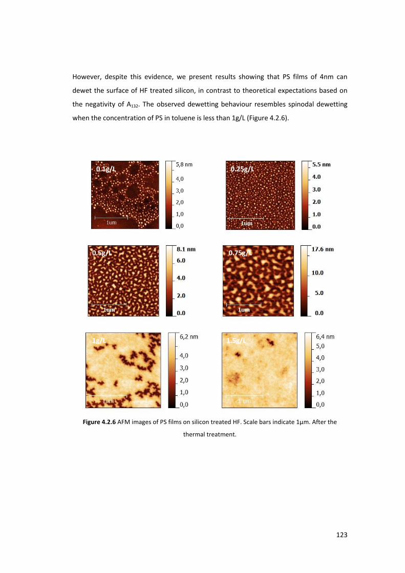
123

However, despite this evidence, we present results showing that PS films of 4nm can

dewet the surface of HF treated silicon, in contrast to theoretical expectations based on

the negativity of A132. The observed dewetting behaviour resembles spinodal dewetting

when the concentration of PS in toluene is less than 1g/L (Figure 4.2.6).

Figure 4.2.6 AFM images of PS films on silicon treated HF. Scale bars indicate 1µm. After the

thermal treatment.

0.1g/L 0.25g/L

0.5g/L 0.75g/L

1g/L 1.5g/L

124

0.00 0.25 0.50 0.75 1.00 1.25 1.50

80

120

160

2001

2

3

4

5

6

20

40

60

80

100

(n

m)

Concentration PS/toluene (g/L)

h0(n

m)

co

ve

rag

e r

ate

(%)

Figure 4.2.7 a) Coverage rate obtained from the AFM image for various concentrations PS/toluene.

b) Average thickness h0 (After the thermal treatment) calculated from the AFM height profile c)

Wavelength calculated from Fourier transform from AFM images.

The discrepancy between the observed results and the theoretical prediction suggests

that either additional forces or a different model have to be considered to probe the

stability of the film :

- A first assumption is the possible existence of a silica layer covering the surface. It

has been reported in the literature that after a HF treatment, the silicon surface is

not stable [Li2002, Graf1990]. This is due to the quick oxidation of the surface of

silicon in contact with air. This fact suggests the formation of a very thin film of

silica over the surface before the polymer deposition. The thickness reported in

the literature is ranging from 0.6 up 0.8 nm of silica in the interval of 10min of

exposure in air.

In this case the effective intermolecular potential is given by equation [eq. 4.1.10]

in which the values from table 4.1.3 are introduced. The potential Ф(h) and its

second derivative Ф h a e plotted i the Figu e . . for PS film thicknesses up

to 6 nm . Ф h < takes pla e at hC=2.1nm. Hence, according to eq. 4.1.10, PS

fil thi e tha h should de et spo ta eousl . This esult does ot o espond

exactly to the observation made by AFM, where islands were formed for

thicknesses less than hC=4.5 nm.

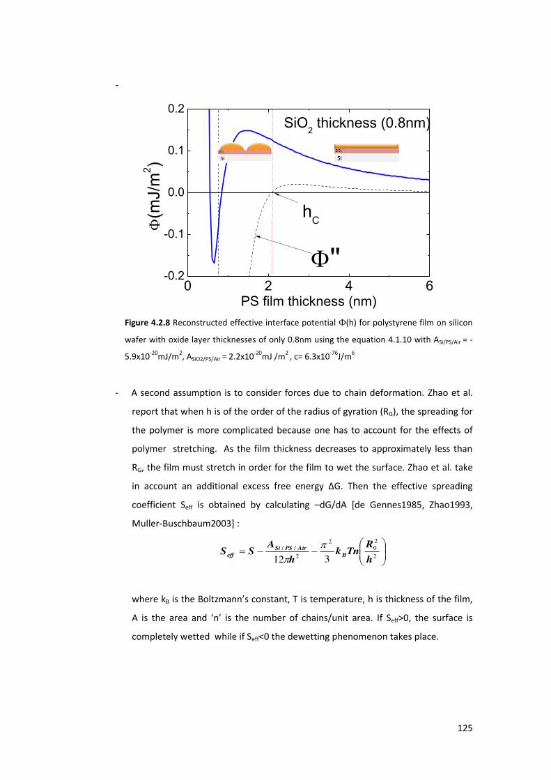
125

-

0 2 4 6-0.2

-0.1

0.0

0.1

0.2

''

(m

J/m

2)

PS film thickness (nm)

SiO2 thickness (0.8nm)

hC

Figure 4.2.8 Reconstructed effective interface potential Ф(h) for polystyrene film on silicon

wafer with oxide layer thicknesses of only 0.8nm using the equation 4.1.10 with ASi/PS/Air = -

5.9x10-20mJ/m2, ASiO2/PS/Air = 2.2x10-20mJ /m2 , c= 6.3x10-76J/m6

- A second assumption is to consider forces due to chain deformation. Zhao et al.

report that when h is of the order of the radius of gyration (RG), the spreading for

the polymer is more complicated because one has to account for the effects of

polymer stretching. As the film thickness decreases to approximately less than

RG, the film must stretch in order for the film to wet the surface. Zhao et al. take

i a ou t a additio al e ess f ee e e g ΔG. The the effe ti e sp eadi g

coefficient Seff is obtained by calculating –dG/dA [de Gennes1985, Zhao1993,

Muller-Buschbaum2003] :

2

20

2

2//

312 h

RTnk

h

ASS B

AirPSSi

eff

where kB is the Boltz a s o sta t, T is te pe atu e, h is thi k ess of the fil ,

A is the a ea a d is the u e of hai s/u it a ea. If Seff>0, the surface is

completely wetted while if Seff<0 the dewetting phenomenon takes place.

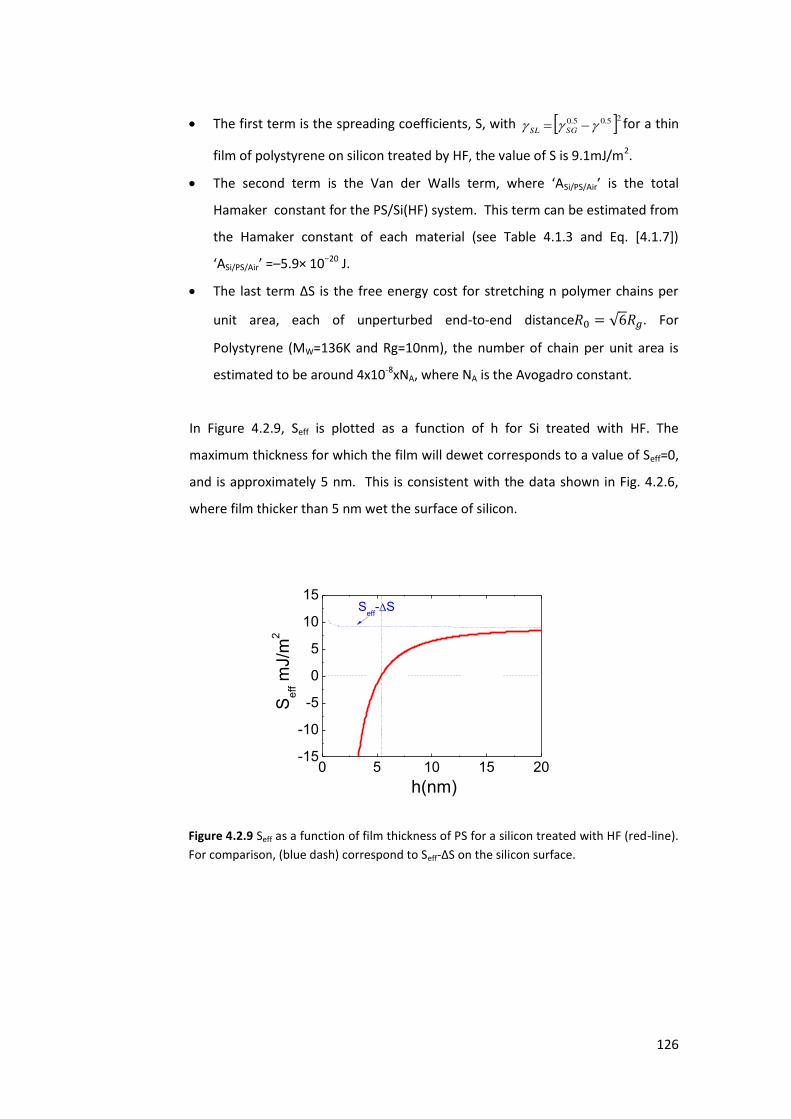
126

The first term is the spreading coefficients, S, with 25.05.0 SGSLfor a thin

film of polystyrene on silicon treated by HF, the value of S is 9.1mJ/m2.

The se o d te is the Va de Walls te , he e ASi/PS/Air is the total

Hamaker constant for the PS/Si(HF) system. This term can be estimated from

the Hamaker constant of each material (see Table 4.1.3 and Eq. [4.1.7])

ASi/PS/Air =–5.9× 10−20 J.

The last te ∆“ is the f ee e e g ost fo st et hi g pol e hai s pe

unit area, each of unperturbed end-to-end distance . For

Polystyrene (MW=136K and Rg=10nm), the number of chain per unit area is

estimated to be around 4x10-8xNA, where NA is the Avogadro constant.

In Figure 4.2.9, Seff is plotted as a function of h for Si treated with HF. The

maximum thickness for which the film will dewet corresponds to a value of Seff=0,

and is approximately 5 nm. This is consistent with the data shown in Fig. 4.2.6,

where film thicker than 5 nm wet the surface of silicon.

0 5 10 15 20-15

-10

-5

0

5

10

15

Se

ff m

J/m

2

h(nm)

Seff

-S

Figure 4.2.9 Seff as a function of film thickness of PS for a silicon treated with HF (red-line).

For comparison, (blue dash) correspond to Seff-Δ“ o the sili o su fa e.

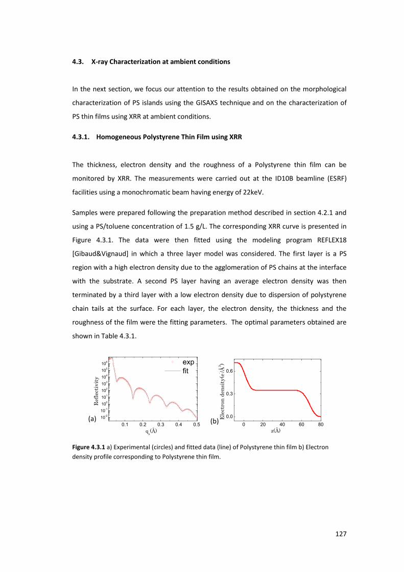
127

4.3. X-ray Characterization at ambient conditions

In the next section, we focus our attention to the results obtained on the morphological

characterization of PS islands using the GISAXS technique and on the characterization of

PS thin films using XRR at ambient conditions.

4.3.1. Homogeneous Polystyrene Thin Film using XRR

The thickness, electron density and the roughness of a Polystyrene thin film can be

monitored by XRR. The measurements were carried out at the ID10B beamline (ESRF)

facilities using a monochromatic beam having energy of 22keV.

Samples were prepared following the preparation method described in section 4.2.1 and

using a PS/toluene concentration of 1.5 g/L. The corresponding XRR curve is presented in

Figure 4.3.1. The data were then fitted using the modeling program REFLEX18

[Gibaud&Vignaud] in which a three layer model was considered. The first layer is a PS

region with a high electron density due to the agglomeration of PS chains at the interface

with the substrate. A second PS layer having an average electron density was then

terminated by a third layer with a low electron density due to dispersion of polystyrene

chain tails at the surface. For each layer, the electron density, the thickness and the

roughness of the film were the fitting parameters. The optimal parameters obtained are

shown in Table 4.3.1.

0.1 0.2 0.3 0.4 0.5

10-2

10-1

100

101

102

103

104

105

106 exp

fit

Ref

lect

ivit

y

qz(Å)

0 20 40 60 80

0.0

0.3

0.6

Ele

ctro

n d

ensi

ty(e

- /Å3 )

z(Å)

Figure 4.3.1 a) Experimental (circles) and fitted data (line) of Polystyrene thin film b) Electron

density profile corresponding to Polystyrene thin film.

(a) (b)

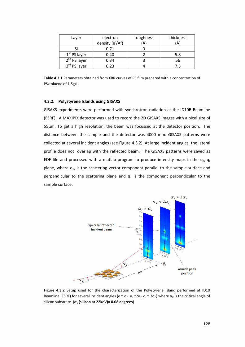
128

Layer electron density (e-/A3)

roughness (Å)

thickness (Å)

Si 0.71 3 - 1st PS layer 0.40 2 5.8 2nd PS layer 0.34 3 56 3rd PS layer 0.23 4 7.5

Table 4.3.1 Parameters obtained from XRR curves of PS film prepared with a concentration of

PS/toluene of 1.5g/L.

4.3.2. Polystyrene Islands using GISAXS

GISAXS experiments were performed with synchrotron radiation at the ID10B Beamline

(ESRF). A MAXIPIX detector was used to record the 2D GISAXS images with a pixel size of

55µm. To get a high resolution, the beam was focussed at the detector position. The

distance between the sample and the detector was 4000 mm. GISAXS patterns were

collected at several incident angles (see Figure 4.3.2). At large incident angles, the lateral

profile does not overlap with the reflected beam. The GISAXS patterns were saved as

EDF file and processed with a matlab program to produce intensity maps in the qxy-qz

plane, where qxy is the scattering vector component parallel to the sample surface and

perpendicular to the scattering plane and qz is the component perpendicular to the

sample surface.

Figure 4.3.2 Setup used for the characterization of the Polystyrene Island performed at ID10

Bea li e E“‘F fo se e al i ide t a gles αi~ αC , αi ~ αC, αi ~ αC he e αC is the critical angle of

silicon substrate. (αC (silicon at 22keV)= 0.08 degrees)

129

Figure 4.3.2 shows the measured GISAXS pattern at ambient conditions as a function of

both wave vector transfers qxy and qz parallel and perpendicular to the surface of the

substrate at an incident angle at αi ≈αC, αi ≈ αC and αi ≈ αC. The GISAXS patterns exhibit a

specular rod that is partially masked by the beam stop and a very intense elongated spot

due to the specularly reflected incident beam which can be seen close to qz= si αi / .

More interestingly are the 2 off-specular truncation rods located at qxy=±0.007A-1 on each

side of the specular rod. The qxy position of such rods is characteristic of the average

distance between the pair neighboring islands. The rod extension along qz is inversely

proportional to the islands height. The line shape of the qz scan (2D image cut at a fixed qxy

position) is strongly depending on the morphology of the islands which can be obtained

by a correct model and a fit to the data.

It is important to highlight that GISAXS patterns need to be measured at an angle of

incidence high enough to avoid a strong signal contamination coming from the foot of the

incident reflected beam in the diffuse scattering. The reflected beam is indeed very

intense compare to the scattered beam but its intensity decays very fast along qz. In this

case as the distance between the islands is quite large, the diffuse rods are located very

close to the specular ridge so that the beam spilling is even more problematic.

Information about the morphology of PS islands can be extracted from line cuts along the

qz and qxy of the GISAXS images (Fig. 4.3.6). We have selected at αi =0.05° a vertical cut at

I(qz,qxy=0.0075 Å-1) and a horizontal cut at I(qxy,qz=0.025 Å-1) and at αi =0.18° a vertical cut

I(qz,qxy=0.0075 Å-1) and a horizontal cut I(qy,qz=0.05 Å-1).

Hemispherical and cylindrical morphologies were chosen to model the particles shapes.

We have also considered the effect of absence (or presence) of a PS residual layer (see

Figure 4.3.3). The fitting parameters included in our model were the radius and height of

islands, the neighboring distance of islands and thickness and electron density of the

residual layer.

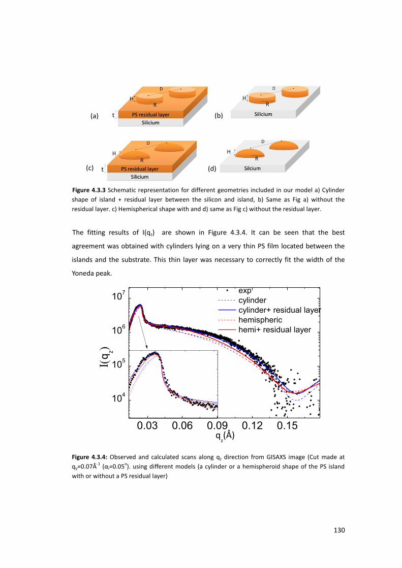
130

Figure 4.3.3 Schematic representation for different geometries included in our model a) Cylinder

shape of island + residual layer between the silicon and island, b) Same as Fig a) without the

residual layer. c) Hemispherical shape with and d) same as Fig c) without the residual layer.

The fitting results of I(qz) are shown in Figure 4.3.4. It can be seen that the best

agreement was obtained with cylinders lying on a very thin PS film located between the

islands and the substrate. This thin layer was necessary to correctly fit the width of the

Yoneda peak.

0.03 0.06 0.09 0.12 0.15

104

105

106

107 exp

cylinder

cylinder+ residual layer

hemispheric

hemi+ residual layer

q

z

qz(Å)

Figure 4.3.4: Observed and calculated scans along qz direction from GISAXS image (Cut made at

qy=0.07Å-1 αi=0.05o). using different models (a cylinder or a hemispheroid shape of the PS island

with or without a PS residual layer)

(a) (b)

(c) (d)

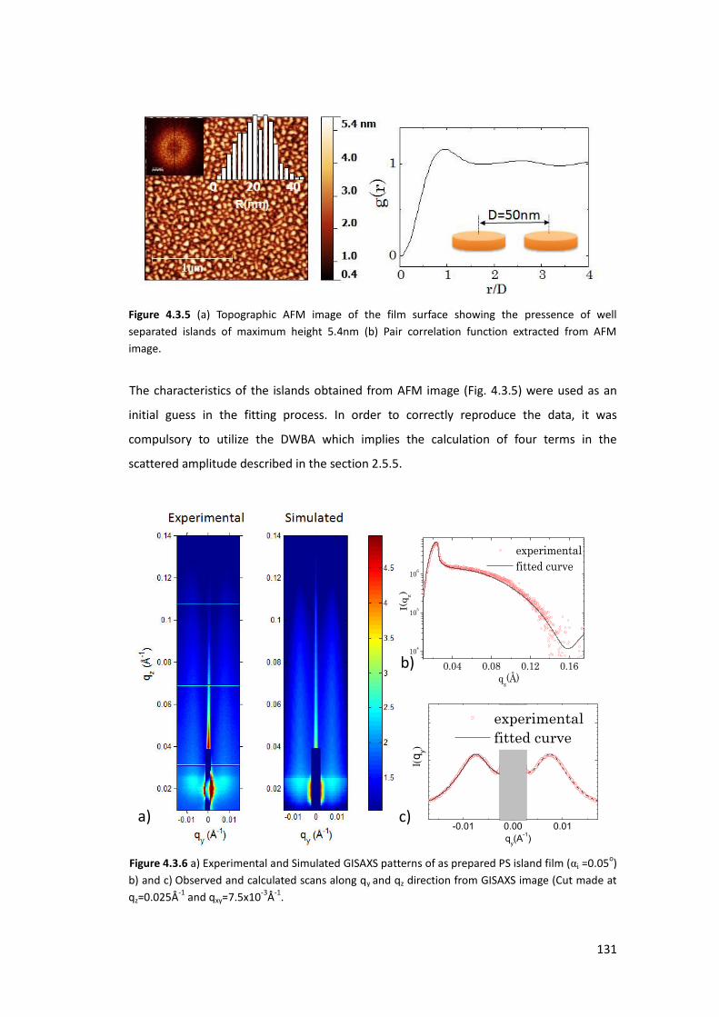
131

Figure 4.3.5 (a) Topographic AFM image of the film surface showing the pressence of well

separated islands of maximum height 5.4nm (b) Pair correlation function extracted from AFM

image.

The characteristics of the islands obtained from AFM image (Fig. 4.3.5) were used as an

initial guess in the fitting process. In order to correctly reproduce the data, it was

compulsory to utilize the DWBA which implies the calculation of four terms in the

scattered amplitude described in the section 2.5.5.

-0.01 0.00 0.01

q

y

qy(A

-1)

experimental fitted curve

Figure 4.3.6 a) Experimental and Simulated GISAXS patterns of as prepared PS island film (αi =0.05o)

b) and c) Observed and calculated scans along qy and qz direction from GISAXS image (Cut made at

qz=0.025Å-1 and qxy=7.5x10-3Å-1.

0.04 0.08 0.12 0.16

104

105

106

experimental fitted curve

I(q

z)

qz(Å)

a)

b)

c)

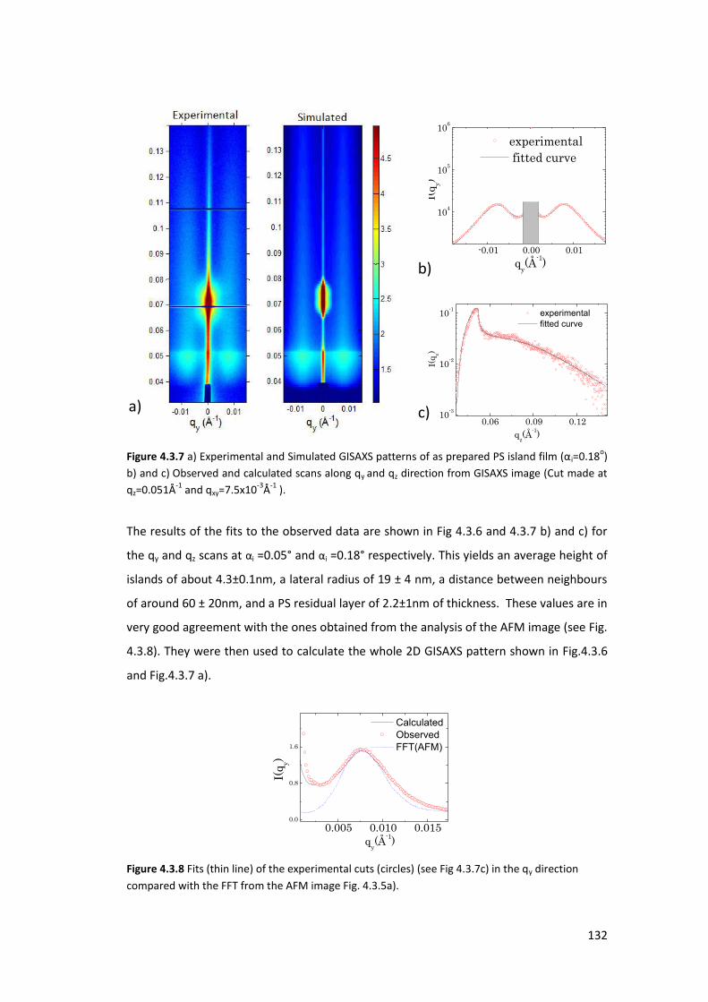
132

-0.01 0.00 0.01

104

105

106

I(q y)

qy(Å

-1)

experimental fitted curve

0.06 0.09 0.1210

-3

10-2

10-1

experimental

fitted curve

I(q z)

qz(Å

-1)

Figure 4.3.7 a E pe i e tal a d “i ulated GI“AX“ patte s of as p epa ed P“ isla d fil αi=0.18o)

b) and c) Observed and calculated scans along qy and qz direction from GISAXS image (Cut made at

qz=0.051Å-1 and qxy=7.5x10-3Å-1 ).

The results of the fits to the observed data are shown in Fig 4.3.6 and 4.3.7 b) and c) for

the qy and qz scans at αi =0.05° and αi =0.18° respectively. This yields an average height of

islands of about 4.3±0.1nm, a lateral radius of 19 ± 4 nm, a distance between neighbours

of around 60 ± 20nm, and a PS residual layer of 2.2±1nm of thickness. These values are in

very good agreement with the ones obtained from the analysis of the AFM image (see Fig.

4.3.8). They were then used to calculate the whole 2D GISAXS pattern shown in Fig.4.3.6

and Fig.4.3.7 a).

0.005 0.010 0.0150.0

0.8

1.6

Calculated

Observed

FFT(AFM)

I(q y)

qy(Å

-1)

Figure 4.3.8 Fits (thin line) of the experimental cuts (circles) (see Fig 4.3.7c) in the qy direction

compared with the FFT from the AFM image Fig. 4.3.5a).

c) a)

b)

133

Residual wetting layer

In order to confirm the existence of the residual wetting layer , the sample was

rinsed in toluene for 10 min. In Figure 4.3.9 we oberve the AFM image of the PS

islands before and after rinsing the sample with toluene. The toluene rinsing

should disolve and remove all the Polystyrene present on the sample. However, a

residual layer is always observed which has a thickness of about h ~2 nm (see

Figure 4.3.9c). The AFM phase image showed in Figure 4.3.9b and 4.3.9c suggests

that this residual layer is covering all the surface of silicon and is present before

and after the toluene rinsing.

Figure 4.3.9 Polystyrene island using a solution of 0.5g/L a) AFM amplitude b) Phase

before rinsing c) AFM amplitude and d) phase after rinsing the sample for 10 min with

toluene.

AFM provides clear information about the dewetting process of the Polystyrene on silicon

under normal environmental conditions. The next step of this study was to investigate the

behavior of these islands when they are exposed to CO2 with pressure conditions ranging

from 0 bar to the pressure corresponding to the supercritical state. These experiments

were carried out in a dedicated cell that was mounted on the diffractometer of the ID10

beam line (ESRF). This cell allows to carrying out in-situ GISAXS and XRR measurements as

(b) (a)

(d) (c)

Amplitude Phase

Amplitude Phase

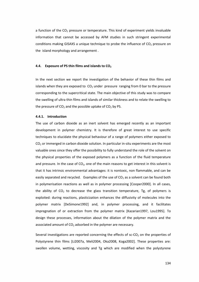
134

a function of the CO2 pressure or temperature. This kind of experiment yields invaluable

information that cannot be accessed by AFM studies in such stringent experimental

conditions making GISAXS a unique technique to probe the influence of CO2 pressure on

the island morphology and arrangement .

4.4. Exposure of PS thin films and islands to CO2

In the next section we report the investigation of the behavior of these thin films and

islands when they are exposed to CO2 under pressure ranging from 0 bar to the pressure

corresponding to the supercritical state. The main objective of this study was to compare

the swelling of ultra thin films and islands of similar thickness and to relate the swelling to

the pressure of CO2 and the possible uptake of CO2 by PS.

4.4.1. Introduction

The use of carbon dioxide as an inert solvent has emerged recently as an important

development in polymer chemistry. It is therefore of great interest to use specific

techniques to elucidate the physical behaviour of a range of polymers either exposed to

CO2 or immerged in carbon dioxide solution. In particular in-situ experiments are the most

valuable ones since they offer the possibility to fully understand the role of the solvent on

the physical properties of the exposed polymers as a function of the fluid temperature

and pressure. In the case of CO2, one of the main reasons to get interest in this solvent is

that it has intrinsic environmental advantages: it is nontoxic, non flammable, and can be

easily separated and recycled. Examples of the use of CO2 as a solvent can be found both

in polymerisation reactions as well as in polymer processing [Cooper2000]. In all cases,

the ability of CO2 to decrease the glass transition temperature, Tg, of polymers is

exploited: during reactions, plasticization enhances the diffusivity of molecules into the

polymer matrix [DeSimone1992] and, in polymer processing, and it facilitates

impregnation of or extraction from the polymer matrix [Kazarian1997, Lou1995]. To

design these processes, information about the dilation of the polymer matrix and the

associated amount of CO2 adsorbed in the polymer are necessary.

Several investigations are reported concerning the effects of sc-CO2 on the properties of

Polystyrene thin films [Li2007a, Meli2004, Oka2008, Koga2002]. These properties are:

swollen volume, wetting, viscosity and Tg which are modified when the polystyrene

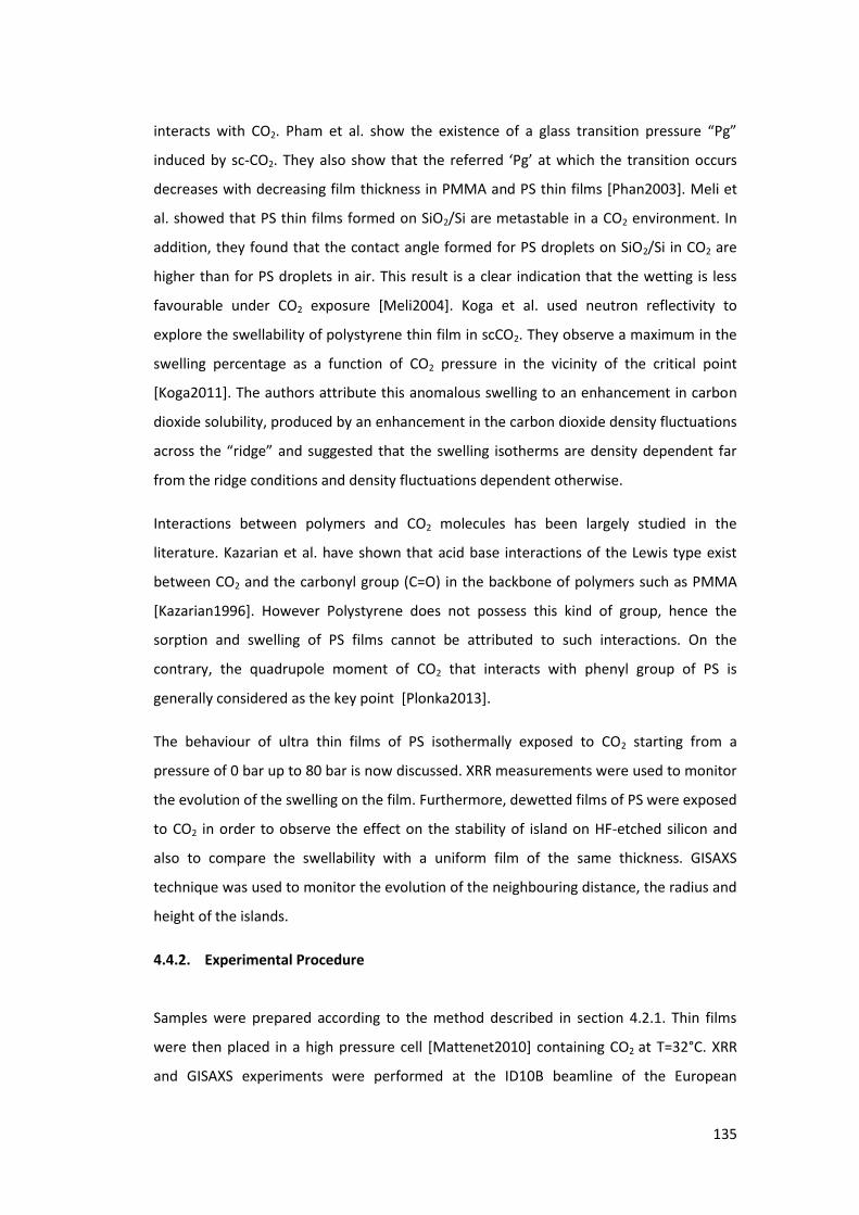
135

interacts with CO2. Pha et al. sho the e iste e of a glass t a sitio p essu e Pg

induced by sc-CO2. They also sho that the efe ed Pg at hi h the t a sitio o u s

decreases with decreasing film thickness in PMMA and PS thin films [Phan2003]. Meli et

al. showed that PS thin films formed on SiO2/Si are metastable in a CO2 environment. In

addition, they found that the contact angle formed for PS droplets on SiO2/Si in CO2 are

higher than for PS droplets in air. This result is a clear indication that the wetting is less

favourable under CO2 exposure [Meli2004]. Koga et al. used neutron reflectivity to

explore the swellability of polystyrene thin film in scCO2. They observe a maximum in the

swelling percentage as a function of CO2 pressure in the vicinity of the critical point

[Koga2011]. The authors attribute this anomalous swelling to an enhancement in carbon

dioxide solubility, produced by an enhancement in the carbon dioxide density fluctuations

a oss the idge a d suggested that the s elli g isothe s a e de sit depe de t fa

from the ridge conditions and density fluctuations dependent otherwise.

Interactions between polymers and CO2 molecules has been largely studied in the

literature. Kazarian et al. have shown that acid base interactions of the Lewis type exist

between CO2 and the carbonyl group (C=O) in the backbone of polymers such as PMMA

[Kazarian1996]. However Polystyrene does not possess this kind of group, hence the

sorption and swelling of PS films cannot be attributed to such interactions. On the

contrary, the quadrupole moment of CO2 that interacts with phenyl group of PS is

generally considered as the key point [Plonka2013].

The behaviour of ultra thin films of PS isothermally exposed to CO2 starting from a

pressure of 0 bar up to 80 bar is now discussed. XRR measurements were used to monitor

the evolution of the swelling on the film. Furthermore, dewetted films of PS were exposed

to CO2 in order to observe the effect on the stability of island on HF-etched silicon and

also to compare the swellability with a uniform film of the same thickness. GISAXS

technique was used to monitor the evolution of the neighbouring distance, the radius and

height of the islands.

4.4.2. Experimental Procedure

Samples were prepared according to the method described in section 4.2.1. Thin films

were then placed in a high pressure cell [Mattenet2010] containing CO2 at T=32°C. XRR

and GISAXS experiments were performed at the ID10B beamline of the European

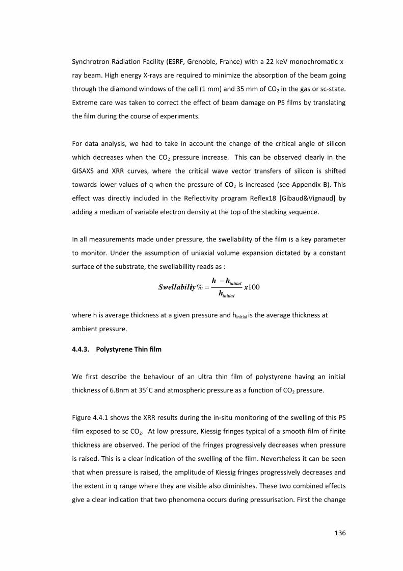
136

Synchrotron Radiation Facility (ESRF, Grenoble, France) with a 22 keV monochromatic x-

ray beam. High energy X-rays are required to minimize the absorption of the beam going

through the diamond windows of the cell (1 mm) and 35 mm of CO2 in the gas or sc-state.

Extreme care was taken to correct the effect of beam damage on PS films by translating

the film during the course of experiments.

For data analysis, we had to take in account the change of the critical angle of silicon

which decreases when the CO2 pressure increase. This can be observed clearly in the

GISAXS and XRR curves, where the critical wave vector transfers of silicon is shifted

towards lower values of q when the pressure of CO2 is increased (see Appendix B). This

effect was directly included in the Reflectivity program Reflex18 [Gibaud&Vignaud] by

adding a medium of variable electron density at the top of the stacking sequence.

In all measurements made under pressure, the swellability of the film is a key parameter

to monitor. Under the assumption of uniaxial volume expansion dictated by a constant

surface of the substrate, the swellabillity reads as :

100% xh

hhtySwellabili

initial

initial

where h is average thickness at a given pressure and hinitial is the average thickness at

ambient pressure.

4.4.3. Polystyrene Thin film

We first describe the behaviour of an ultra thin film of polystyrene having an initial

thickness of 6.8nm at 35°C and atmospheric pressure as a function of CO2 pressure.

Figure 4.4.1 shows the XRR results during the in-situ monitoring of the swelling of this PS

film exposed to sc CO2. At low pressure, Kiessig fringes typical of a smooth film of finite

thickness are observed. The period of the fringes progressively decreases when pressure

is raised. This is a clear indication of the swelling of the film. Nevertheless it can be seen

that when pressure is raised, the amplitude of Kiessig fringes progressively decreases and

the extent in q range where they are visible also diminishes. These two combined effects

give a clear indication that two phenomena occurs during pressurisation. First the change

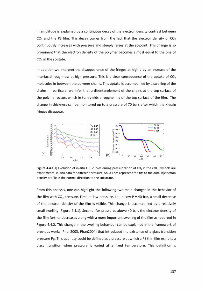
137

in amplitude is explained by a continuous decay of the electron density contrast between

CO2 and the PS film. This decay comes from the fact that the electron density of CO2

continuously increases with pressure and steeply raises at the sc-point. This change is so

prominent that the electron density of the polymer becomes almost equal to the one of

CO2 in the sc-state.

In addition we interpret the disappearance of the fringes at high q by an increase of the

interfacial roughness at high pressure. This is a clear consequence of the uptake of CO2

molecules in between the polymer chains. This uptake is accompanied by a swelling of the

chains. In particular we infer that a disentanglement of the chains at the top surface of

the polymer occurs which in turn yields a roughening of the top surface of the film. The

change in thickness can be monitored up to a pressure of 70 bars after which the Kiessig

fringes disappear.

0.1 0.2 0.3 0.4

10-3

10-2

10-1

100

101

102

103

104

105

106

107

108

109

1010

1011

1012

1013

70 bar

45 bar

30 bar

0 bar

Ref

lect

ivit

y

qz(Å)

0 20 40 60 80 100 120

0.0

0.1

0.2

0.3

0.4

0.5

0.6

0.7 70 bar

30 bar

0 bar

Ele

ctro

n d

ensi

ty(e

- /Å3 )

z(Å)

Figure 4.4.1 a) Evolution of in-situ XRR curves during pressurization of CO2 in the cell. Symbols are

experimental in-situ data for different pressure. Solid lines represent the fits to the data. b)electron

density profile in the normal direction to the substrate.

From this analysis, one can highlight the following two main changes in the behavior of

the film with CO2 pressure. First, at low pressure, i.e., below P = 40 bar, a small decrease

of the electron density of the film is visible. This change is accompanied by a relatively

small swelling (Figure 4.4.1). Second, for pressures above 40 bar, the electron density of

the film further decreases along with a more important swelling of the film as reported in

Figure 4.4.2. This change in the swelling behaviour can be explained in the framework of

previous works [Phan2003, Phan2004] that introduced the existence of a glass transition

pressure Pg. This quantity could be defined as a pressure at which a PS thin film exhibits a

glass transition when pressure is varied at a fixed temperature. This definition is

(a) (b)

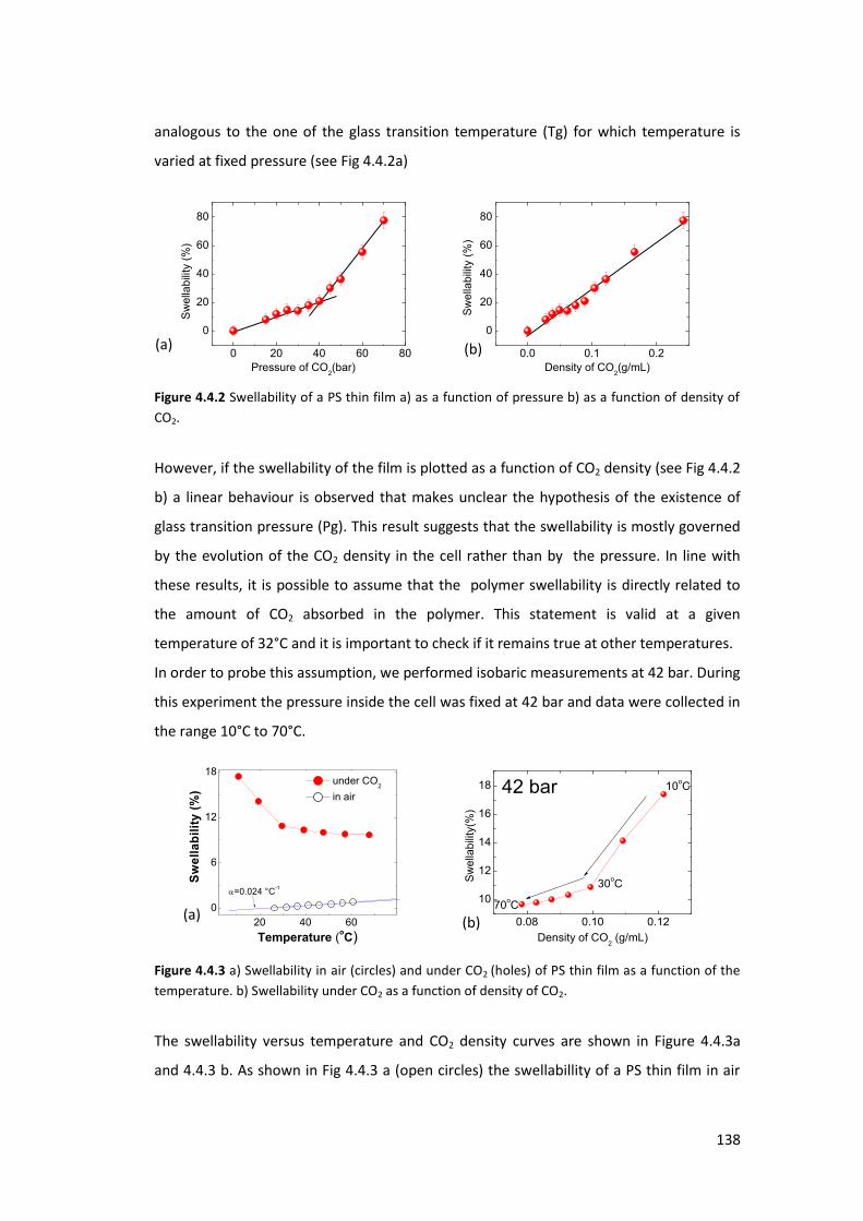
138

analogous to the one of the glass transition temperature (Tg) for which temperature is

varied at fixed pressure (see Fig 4.4.2a)

0 20 40 60 80

0

20

40

60

80

S

we

llab

ility

(%

)

Pressure of CO2(bar)

0.0 0.1 0.2

0

20

40

60

80

Sw

ella

bili

ty (

%)

Density of CO2(g/mL)

Figure 4.4.2 Swellability of a PS thin film a) as a function of pressure b) as a function of density of

CO2.

However, if the swellability of the film is plotted as a function of CO2 density (see Fig 4.4.2

b) a linear behaviour is observed that makes unclear the hypothesis of the existence of

glass transition pressure (Pg). This result suggests that the swellability is mostly governed

by the evolution of the CO2 density in the cell rather than by the pressure. In line with

these results, it is possible to assume that the polymer swellability is directly related to

the amount of CO2 absorbed in the polymer. This statement is valid at a given

temperature of 32°C and it is important to check if it remains true at other temperatures.

In order to probe this assumption, we performed isobaric measurements at 42 bar. During

this experiment the pressure inside the cell was fixed at 42 bar and data were collected in

the range 10°C to 70°C.

20 40 60

0

6

12

18 under CO

2

in air

Sw

ell

ab

ilit

y (

%)

Temperature (oC)

=0.024 °C-1

0.08 0.10 0.12

10

12

14

16

18

70oC

Sw

ella

bili

ty(%

)

Density of CO2 (g/mL)

30oC

10oC42 bar

Figure 4.4.3 a) Swellability in air (circles) and under CO2 (holes) of PS thin film as a function of the

temperature. b) Swellability under CO2 as a function of density of CO2.

The swellability versus temperature and CO2 density curves are shown in Figure 4.4.3a

and 4.4.3 b. As shown in Fig 4.4.3 a (open circles) the swellabillity of a PS thin film in air

(a) (b)

(a) (b)

139

slightly increases when temperature is raised. This behaviour is typically expected when a

material is heated. It allows to define the coefficient of thermal expansion (CTE) of the

material which for PS in air is found to be α= . °C-1. When PS is heated under CO2 at a

constant pressure P=42bar, the swellability (shown in full red circles) is drastically

different. We clearly observe a decrease of the swellability when the temperature is

increased. This yields a negative non linear CTE at this pressure. Once again this shows

that the thermodynamical parameters (T, P) are not sufficient to explain the behaviour of

the swellability.

If we now plot the evolution of the swellability versus the density of CO2 we clearly

observe that the swellability is not linear with the density of CO2 (see Fig 4.4.3b). In

conclusion, these experiments clearly evidence that the behaviour of a thin film of PS

exposed to CO2 under pressure is quite difficult to parameterize. The isothermal

swellabillity is linear with the density while the isobar swellabilty is not.

So far these two experiments do not allow any firm conclusion and further experiments

are needed to fully understand these observations.

4.4.4. Polystyrene Islands

We now consider the structural stability of PS islands of average thickness 1.72 nm

supported by HF-etched Silicon in CO2 environments at 32°C.

Figure 4.4.4, shows the GISAXS results during the in-situ monitoring of the morphology of

islands when they are exposed to CO2. One of the main changes is the extension of the 2-

off specular rods located at qxy = 0.007 Å-1 which decreases progressively as the pressure

is increased. On the other hand, it is observed that the qy position of each specular rod is

fixed at all pressures. In addition to these two phenomena, a decrease in the contrast due

to the increase in the CO2 electron density is observed. In order to analyze these changes

in more detail, we have performed linear cuts in the GISAXS images to extract information

about the evolution of the morphological parameters. A vertical cut I(qz) at qxy=0.0075Å-1

f o the GI“AX“ i age at αi=0.05° and a horizontal cut I(qy) at qz=0.05 Å-1 from the

GISAXS image at αi =0.18° were used to fit the data.

140

Figure 4.4.4 Experimental GISAXS patterns of PS islands at increasing CO2 pressures.

At low pressure, polysdisperse islands with a cylindrical shape on a very thin film of PS

were first considered in the fitting (see Fig. 4.4.5). Then at higher pressure, since islands

are hyper swelling in the z direction while they do not swell laterally, we have considered

that the central part of the island could swell more than the outer part and therefore we

have assumed a hemispherical shape. Such an assumption was also motivated by the

impossibility to properly fit the observed data to a cylindrical shape for the islands.

.

Figure 4.4.5 A cylindrical and hemispherical shape on a PS thin film.

Figure 4.4.6 shows the scattering curves in the qz direction during the in-situ monitoring of

the swelling of the PS islands exposed to CO2. From this figure, we can clearly see that the

location of the first minimum in the qz-cut progressively decreases when the CO2 pressure

increases. This is the clear signature that the height of the islands increases.

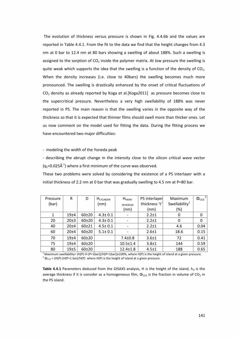
141

The evolution of thickness versus pressure is shown in Fig. 4.4.6b and the values are

reported in Table 4.4.1. From the fit to the data we find that the height changes from 4.3

nm at 0 bar to 12.4 nm at 80 bars showing a swelling of about 188%. Such a swelling is

assigned to the sorption of CO2 inside the polymer matrix. At low pressure the swelling is

quite weak which supports the idea that the swelling is a function of the density of CO2.

When the density increases (i.e. close to 40bars) the swelling becomes much more

pronounced. The swelling is drastically enhanced by the onset of critical fluctuations of

CO2 density as already reported by Koga et al.[Koga2011] as pressure becomes close to

the supercritical pressure. Nevertheless a very high swellability of 188% was never

reported in PS. The main reason is that the swelling varies in the opposite way of the

thickness so that it is expected that thinner films should swell more than thicker ones. Let

us now comment on the model used for fitting the data. During the fitting process we

have encountered two major difficulties:

- modeling the width of the Yoneda peak

- describing the abrupt change in the intensity close to the silicon critical wave vector

(qz=0.025Å-1) where a first minimum of the curve was observed.

These two problems were solved by considering the existence of a PS interlayer with a

initial thickness of 2.2 nm at 0 bar that was gradually swelling to 4.5 nm at P=80 bar.

Pressure (bar)

R D HCYLINDER (nm)

HHEMI-

SPHEROID

(nm)

PS interlayer

thi k ess t (nm)

Maximum Swellability1

(%)

ΦCO2 2

1 19±4 60±20 4.3± 0.1 - 2.2±1 0 0 20 20±3 60±20 4.3± 0.1 - 2.2±1 0 0 40 20±4 60±21 4.5± 0.1 - 2.2±1 4.6 0.04 60 20±4 60±20 5.1± 0.1 - 2.6±1 18.6 0.15

70 19±4 60±20 7.4±0.8 3.6±1 72 0.41 75 19±4 60±20 10.5±1.4 3.8±1 144 0.59 80 19±5 60±20 12.4±1.8 4.5±1 188 0.65

1 Maximum swellability= (H(P)-H (P=1bar))/H(P=1bar))x100%, where H(P) is the height of island at a given pressure. 2 ΦCO2 ≈ H P -(H(P=1 bar)/H(P) where H(P) is the height of island at a given pressure.

Table 4.4.1 Parameters deduced from the GISAXS analysis, H is the height of the island, h0 is the

average thickness if it is consider as a homogeneous film, ΦCO2 is the fraction in volume of CO2 in

the PS island.

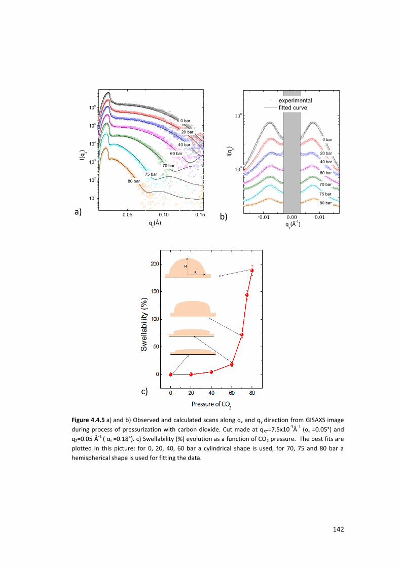
142

Figure 4.4.5 a) and b) Observed and calculated scans along qz and qy direction from GISAXS image

during process of pressurization with carbon dioxide. Cut made at qXY=7.5x10-3Å-1 (αi =0.05°) and

qZ=0.05 Å-1 ( αi =0.18°). c) Swellability (%) evolution as a function of CO2 pressure. The best fits are

plotted in this picture: for 0, 20, 40, 60 bar a cylindrical shape is used, for 70, 75 and 80 bar a

hemispherical shape is used for fitting the data.

0.05 0.10 0.15

101

102

103

104

105

106

80 bar

75 bar

70 bar

60 bar

40 bar

20 bar

I(

qz)

qz(Å)

0 bar

-0.01 0.00 0.01

105

106

80 bar

75 bar

70 bar

60 bar

40 bar

20 bar

I(q

y)q

y(Å

-1)

experimental

fitted curve

0 bar

b) a)

c)

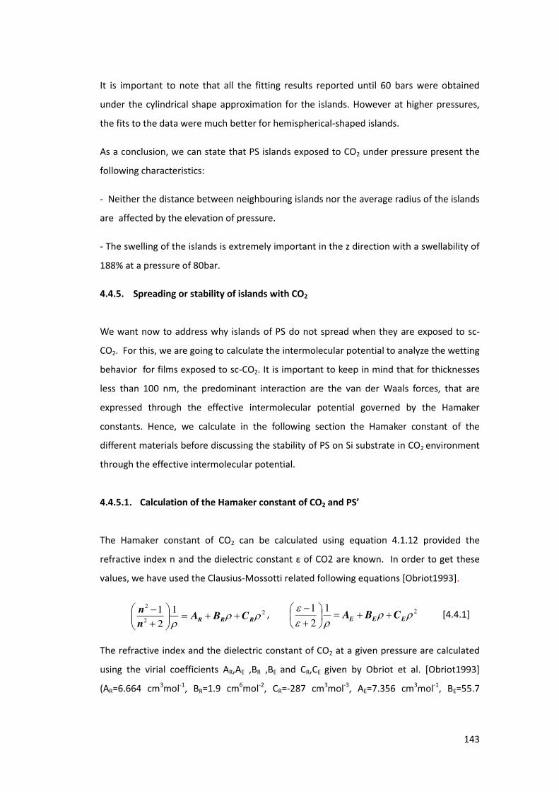
143

It is important to note that all the fitting results reported until 60 bars were obtained

under the cylindrical shape approximation for the islands. However at higher pressures,

the fits to the data were much better for hemispherical-shaped islands.

As a conclusion, we can state that PS islands exposed to CO2 under pressure present the

following characteristics:

- Neither the distance between neighbouring islands nor the average radius of the islands

are affected by the elevation of pressure.

- The swelling of the islands is extremely important in the z direction with a swellability of

188% at a pressure of 80bar.

4.4.5. Spreading or stability of islands with CO2

We want now to address why islands of PS do not spread when they are exposed to sc-

CO2. For this, we are going to calculate the intermolecular potential to analyze the wetting

behavior for films exposed to sc-CO2. It is important to keep in mind that for thicknesses

less than 100 nm, the predominant interaction are the van der Waals forces, that are

expressed through the effective intermolecular potential governed by the Hamaker

constants. Hence, we calculate in the following section the Hamaker constant of the

different materials before discussing the stability of PS on Si substrate in CO2 environment

through the effective intermolecular potential.

4.4.5.1. Calculation of the Hamaker constant of CO2 a d PS

The Hamaker constant of CO2 can be calculated using equation 4.1.12 provided the

refractive index n and the diele t i o sta t of CO2 are known. In order to get these

values, we have used the Clausius-Mossotti related following equations [Obriot1993].

22

2 121

RRR CBAn

n

, 21

21

EEE CBA

[4.4.1]

The refractive index and the dielectric constant of CO2 at a given pressure are calculated

using the virial coefficients AR,AE ,BR ,BE and CR,CE given by Obriot et al. [Obriot1993]

(AR=6.664 cm3mol-1, BR=1.9 cm6mol-2, CR=-287 cm3mol-3, AE=7.356 cm3mol-1, BE=55.7

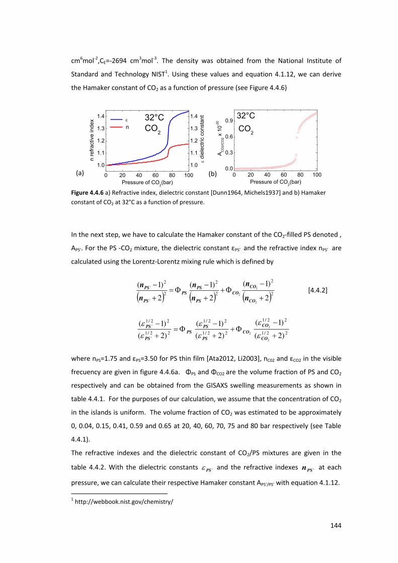
144

cm6mol-2,CE=-2694 cm3mol-3. The density was obtained from the National Institute of

Standard and Technology NIST1. Using these values and equation 4.1.12, we can derive

the Hamaker constant of CO2 as a function of pressure (see Figure 4.4.6)

0 20 40 60 80 100

1.0

1.1

1.2

1.3

1.4

n r

efr

active index

Pressure of CO2(bar)

1.0

1.1

1.2

1.3

1.4

n

d

iele

ctr

ic c

onsta

nt32°C

CO2

0 20 40 60 80 1000.0

0.3

0.6

0.9

CO2

AC

O2/C

O2 x

10

-20

Pressure of CO2(bar)

32°C

Figure 4.4.6 a) Refractive index, dielectric constant [Dunn1964, Michels1937] and b) Hamaker

constant of CO2 at 32°C as a function of pressure.

In the next step, we have to calculate the Hamaker constant of the CO2-filled PS denoted ,

AP“ . For the PS -CO2 i tu e, the diele t i o sta t P“ and the refractive index nP“ are

calculated using the Lorentz-Lorentz mixing rule which is defined by

22

2

2

2

'

2'

2

)1(

2

)1(

2

)1(

2

2

2

CO

CO

CO

PS

PSPS

PS

PS

n

n

n

n

n

n [4.4.2]

22/1

22/1

22/1

22/1

22/1'

22/1'

)2(

)1(

)2(

)1(

)2(

)1(

2

2

2

CO

CO

CO

PS

PS

PS

PS

PS

where nPS= . a d PS=3.50 for PS thin film [Ata2012, Li2003], nC02 a d CO2 in the visible

frecuency are given in figure 4.4.6a. ΦPS a d ΦCO2 are the volume fraction of PS and CO2

respectively and can be obtained from the GISAXS swelling measurements as shown in

table 4.4.1. For the purposes of our calculation, we assume that the concentration of CO2

in the islands is uniform. The volume fraction of CO2 was estimated to be approximately

0, 0.04, 0.15, 0.41, 0.59 and 0.65 at 20, 40, 60, 70, 75 and 80 bar respectively (see Table

4.4.1).

The refractive indexes and the dielectric constant of CO2/PS mixtures are given in the

table 4.4.2. With the dielectric constants 'PS and the refractive indexes 'PSn at each

pressure, we can calculate their respective Hamaker constant AP“ /P“ with equation 4.1.12.

1 http://webbook.nist.gov/chemistry/

(a) (b)

145

Then using the Hamaker constant of each material and replacing them in equation 4.1.8,

e a fi all al ulate the Ha ake o sta t of the s ste “i/P“ /CO2 and SiO2/P“ /CO2

which is given in the table 4.4.2

0 bar 20 bar 40 bar 60 bar 70bar 75 bar 80 bar ΦCO2 0 0 0.04 0.15 0.41 0.59 0.65 nPS 1.75 1.75 1.73 1.67 1.54 1.44 1.42 εPS 3.51 3.51 3.41 3.18 2.65 2.28 2.21 APS -PS x10-20 J 10.7 10.7 10.2 9.02 6.32 4.49 4.13 ASi/PS /CO2 x10-20 J -5.9 -5.9 -5.74 -5.71 -5.54 -4.74 -3.45 ASiO2/PS /CO2 x10-20 J 2.2 2.2 1.9 1.2 -0.12 -0.72 -0.61

Table 4.4.2 Calculation of the Hamaker constant of PS-CO2 mixture. ASI/SI= 25.6x10-20 J and

ASIO2/SIO2=6.6 x10-20 J.

4.4.5.2. Discussions

From Table 4.4.2, it can be observed that the Hamaker constants for ASi/PS /CO2 and

ASiO2/PS /CO2 are influenced by the CO2 olu e f a tio ΦCO2 filled inside the polymer. Hence

the shape of the effective intermolecular potential is also modified.

- If e o side that the s ste is gi e “i HF /P“ /CO2, the Hamaker constant

given in Table 4.4.2 has a negative sign over all the interval of pressures. This

suggests that Polystyrene films on HF treated silicon in a CO2 environment has a

complete wetting behaviour at all the considered pressures. However this is not

what is experimentally observed which rules out this hypothesis.

- If we assume the presence of SiO2 covering the surface due to the quick oxidation

of HF treated silicon, the system becomes composed of four materials

Si/SiO2/P“ /CO2. In section 4.4.2, this consideration gave us a fair explanation for

the appearance of islands instead of a film as the most stable structure in air

condition. For this reason, we also consider this hypothesis as a reasonable

starting point for the study of the stability of PS islands in CO2 environment.

The effective intermolecular potential of the system Si/SiO2/P“ /CO2 is defined as:

2

/'//'/

2

/'/

8 )(1212)( 22222

dh

AA

h

A

h

ch

COPSSiCOPSSiOCOPSSiO

VDW

[4.4.3]

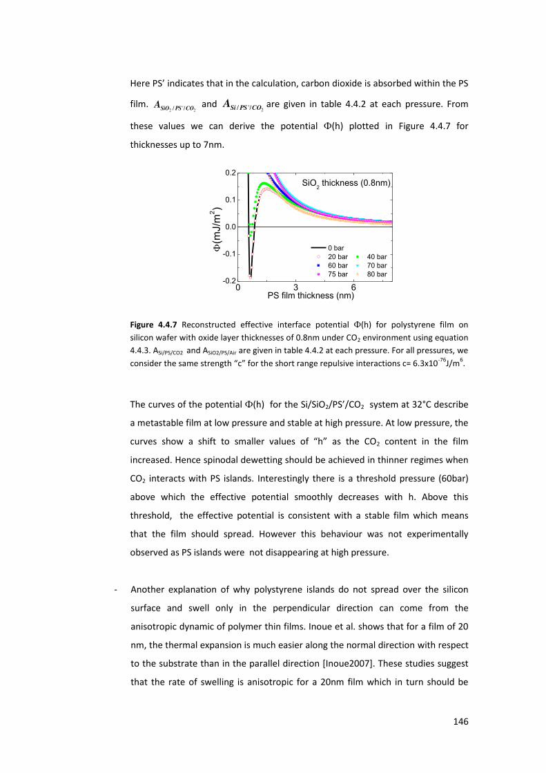
146

He e P“ i di ates that i the al ulatio , a o dio ide is a so ed ithi the P“

film. 22 /'/ COPSSiOA and

2/'/ COPSSiA are given in table 4.4.2 at each pressure. From

these values we can derive the potential Ф(h) plotted in Figure 4.4.7 for

thicknesses up to 7nm.

0 3 6

-0.2

-0.1

0.0

0.1

0.2

0 bar

20 bar 40 bar

60 bar 70 bar

75 bar 80 bar

SiO2 thickness (0.8nm)

(m

J/m

2)

PS film thickness (nm)

Figure 4.4.7 Reconstructed effective interface potential Ф(h) for polystyrene film on

silicon wafer with oxide layer thicknesses of 0.8nm under CO2 environment using equation

4.4.3. ASi/PS/CO2 and ASiO2/PS/Air are given in table 4.4.2 at each pressure. For all pressures, we

o side the sa e st e gth fo the sho t a ge epulsi e i te a tio s = . -76J/m6.

The curves of the potential Ф(h) for the Si/SiO2/P“ /CO2 system at 32°C describe

a metastable film at low pressure and stable at high pressure. At low pressure, the

u es sho a shift to s alle alues of h as the CO2 content in the film

increased. Hence spinodal dewetting should be achieved in thinner regimes when

CO2 interacts with PS islands. Interestingly there is a threshold pressure (60bar)

above which the effective potential smoothly decreases with h. Above this

threshold, the effective potential is consistent with a stable film which means

that the film should spread. However this behaviour was not experimentally

observed as PS islands were not disappearing at high pressure.

- Another explanation of why polystyrene islands do not spread over the silicon

surface and swell only in the perpendicular direction can come from the

anisotropic dynamic of polymer thin films. Inoue et al. shows that for a film of 20

nm, the thermal expansion is much easier along the normal direction with respect

to the substrate than in the parallel direction [Inoue2007]. These studies suggest

that the rate of swelling is anisotropic for a 20nm film which in turn should be

147

even more anisotropic for 5 nm PS islands. This assumption can explain our

observations.

- The last hypothesis lies on the fact that very thin films on the order of h <10nm

may present strong interaction between the substrate (silicon treated with HF)

and the polymers that can dominate over the van der Waals interaction in the

analysis of the stability of PS thin films.

Despite the various hypotheses offered none of them seem to explain clearly and

satisfactorily the observed behaviour. As a conclusion the reason for which islands are

very stable when they are exposed to sc-CO2 is still controversial and deserves further

studies.

In conclusion, we have presented in-situ XRR and GISAXS studies of the swellability as a

function of pressure of Polystyrene confined in one (thin film) and two dimensions

(islands). The results are similar to those reported by other groups confirming that thin

films swell when they are exposed to CO2. However in the case of PS islands, we observe a

much larger swellability than for a homogeneous thin film. This effect can be attributed to

the larger free surface in the island compared with that of thin films which allows for a

greater absorption of CO2. In addition, it was shown that PS islands (h<10 nm) supported

on HF treated silicon do not spread in supercritical CO2 environment. PS islands remain at

a fixed position and grow only in the perpendicular direction.

148

149

Bibliography

[Angell2000] Angell, C.A.; Ngai, K.L.; McKenna, G.B.; McMillan, P.F.; Martin, S.W. J. Appl. Phys.

(2000) 88, 3113.

[Ata2009] Ata, S.; Muramatsu, M.; Takeda, J.; Ohdaira, T.; Suzuki, R.; Ito, K.; Kobayashi, Y.;

Ougizawa, T. Polymer 50 (2009) 3343–3346.

[Ata2012] Ata, S.; Kuboyama, K.; Ito, K.; Kobayashi, Y.; Ougizawa, T., Polymer 53 (2012) 1028-1033.

[Bergeron2000] Bergeron, V.; Bonn, D.; Martin, J. Y.; Vovelle, L. Nature (2000) 405, 772.

[Bertrand2002] Bertrand, E., J. Petrol. Sci. Eng. (2002)33, 217.

[Bonn2009] Bonn, D.; Eggers, J.; Indekeu, J.; Meunier, J.; Rolley, E., Rev. Mod. Phys. (2009) 81, 739,

[Brochard-Wyart1990] Brochard-Wyart, F. Langmuir (1991), 7, 335-338.

[Cohen1959] Cohen, M.H.; Turnbull, D., J. Chem. Phys. (1959) 31 1164.

[Cooper2000] Cooper, A. J Mater Chem (2000) 10, 207–234.

[de Gennes1985] de Gennes P. G., Reviews of Modern Physics, (1985), Vol. 57, No. 3, Part I.

[DeSimone1992] DeSimone, J.; Guan, Z.; Elsbernd, C. Science (1992) 257, 945–947.

[Donth2001] Donth, E. The Glass Transition: Relaxation Dynamics in Liquids and Disordered

Materials, Springer, Berlin, 2001.

[Dublek2004] Dlubek, G.; Kilburn, D.; Bondarenko, V.; Pionteck, J.; Krause-Rehberg, R.; Alam, M. A.,

Positron Annihilation: A Unique Method for Studying Polmers Macromolecular Symposia 210,

Reactive Polymers 2003, Ed. H.-J. Adler, Weinheim, WILEY-VCH, March 2004, p. 11.

[Dunn1964] Dunn, A.F. Canadian Jounal of Physics, (1964) Volume 42.

[Forrest2002] Forrest, J. A., European Physical Journal E: Soft Matter (2002), 8, (2), 261-266.

[Gibaud&Vignaud] G. Vignaud and A. Gibaud, Program REFLEX18, a matlab routine for the

simulation of specular x-ray reflectivity data with the matrix technique.

[Graf1990] Gräf, D.; Grundner, M.; Schulz, R.; Mühlhoff, L. Journal of applied physics, 1990, 68(10),

5155-5161.

[Hsu2000] Hsu, D. T.; Shi, F. G.; Zhao, B.; Brongo, M. In Theory for the thickness dependent glass

transition temperature of amorphous polymer thin films, Proceedings - Electrochemical Society

(2000), 99-7(Low and High Dielectric Constant Materials, and Thin Film Materials for Advanced

Packaging Technologies), (2000) pp 53-61 .

[Jacobs1998] Jacobs, K.; Herminghaus, S.; Mecke, K.R. Langmuir (1998) 14, 965.

[Kazarian1996] Kazarian, S. G.; Vincent, M. F.; Bright, F. V.; Liotta, C. L.; Eckert, C. A. , J. Am. Chem.

Soc. (1996) 118, 1729-1736.

[Koga2002] Koga, T.; Seo, Y. S.; Zhang, Y.; Shin, K.; Kusano, K.; Nishikawa, K.; Rafailovich, M. H.;

Sokolov, J. C.; Chu, B.; Peiffer, D.; Occhiogrosso, R.; Satija, S. K. Phys. Rev. Lett. (2002) 89, 125506.

150

[Koga2004] Koga, T.; Ji, Y.; Seo, Y. S.; Gordon, C.; Qu, F.; Rafailovich, M. H.; Sokolov, J. C.; Satija, S.

K. J. Polym. Sci. B: Polym. Phys. (2004) 42, 3282.

[Koga2003] Koga, T.; Seo, Y. S.; Shin, K.; Zhang, Y.; Rafailovich, M. H.; Sokolov, J. C.; Chu, B.; Satija,

S. K. Macromolecules (2003) 36, 5236.

[Koga2005] Koga, T.; Akashige, E.; Reinstein, A.; Bronner, M.; Seo, Y. S.; Shin, K.; Rafailovich, M. H.;

Sokolov, J. C.; Chu, B.; Satija, S. K. Physica B (2005), 357, 73.

[Koga 2011] Koga, T.; Gin, P.; Yamaguchi, H.; Endoh, M. K.; Asada, M.; Sendogdular, L.; Kobayashi,

M.; Takahara, A.; Akgun, B.; Satija, S. K.; Sumi, T. Polymer (2011) , − .

[Lee1968] Lee, L.H., J. Appl. Polym. Sci., (1968). 12, 719

[Li2002] Li, F.; Balazs, M.K., 21th Annual Semiconductor Pure Water and Chemicals Conference

Proceedings, Santa Clara, CA, March 2002.

[Li2007a] Li, Y.; Park, E. J.; Lim, K. T.; Johnston, K. P.; Green, P. F. Journal of Polymer Science: Part

B: Polymer Physics, Vol. 45, (2007) 1313–1324.

[Li2007] Li, Y.; Pham, J. Q.; Johnston, K. P.; Green, P. F. Langmuir (2007) 23, 9785-9793.

[Lou1995] Lou, X.; Janssen, H.G.; Cramers, C. A. J Microcolumn (1995), 7, 303–317.

[Meli2004] Meli, L.; Pham, J. Q.; Johnston, K. P.; Green, P. F., Physical Review E(2004) 69, 051601.

[Michels1937] Michels, A.; Hamers, J., Physica IV, (1937)10.

[Mukherjee2011] Mukherjee, R.; Sharma, A.; Steiner, U., Surface Instability and Pattern Formation

in Thin Polymer Films Generating Micro- and Nanopatterns on Polymeric Materials. Edited by A.

del Campo and E. Arzt, 2011 WILEY-VCH Verlag GmbH & Co. KGaA, Weinheim.

[Muller-Buschbaum2003] Muller-Buschbaum P., Eur. Phys. J. E (2003)12, 443–448

[Obriot1993] Obriot, J.; Ge, J.; Bose, T.K.; St-Arnaud, J.M., Fluid Phase Equilib. (1993) 86 315–350.

[Oka2008] Oka, T.; Ito, K.; He, C.; Dutriez, C.; Yokoyama, H.; Kobayashi, Y., J. Phys. Chem. B (2008)

112, 12191–12194.

[Phan2003] Pham, J. Q.; Sirard, S.M.; Johnston, K. P.; Green. P. F., Physical Review Letters, (2003)

91, 17, 175503-1.

[Phan2004] Pham, J. Q; Johnston, K. P.; Green, P. F., J. Phys. Chem. B (2004), 108, 3457.

[Plonka2013] Plonka, A. M.; Banerjee, D.; Woerner, W. R.; Zhang, Z.; Nijem, N.; Chabal, Y. J.; Li, J.;

Parise, J. B., Angew. Chem. Int. Ed. (2013), 52, 1692 –1695.

[Seeman2000] Seemann, R.; Herminghaus, S.; Jacobs, K., Phys. Rev. Lett. (2001), 86, 5534.

[Seeman2001] Seemann, R.; Jacobs, K.; Blossey, R. J. Phys.: Condens. Matter, (2001), 13, 4915–

4923.

[Shahidzadeh2003] Shahidzadeh, N.; Bertrand, E.; Dauplait, J.P.; Borgotti, J. C.; D. Bonn, (2003)

Transp. Porous Media 52, 213.

[Struik1977] Struik, L.C.E., Polymer Engineering and Science, (1977) Vol 17, No. 3.

[Tabelin2004] Tabeling, P., Microfluidics (2004); EDP Sciences: Paris.

[Tsui2003] Tsui, O.K.C.; Wang, Y.J.; Zhao, H.; Du, B.,Eur. Phys. J. E (2003) 12, 417–425.

151

[Wu1982] Wu, S., Polymer Interface and Adhesion, Marcel Dekker, New York, NY, 1982, p. 87.

[Zhao1993] Zhao, W.; Rafailovich, M. H.; Sokolov, J.; Fetters, L. J.; Plano, R.; Sanyal, M. K.; Sinha, S.

K.; Sauer , B., Phys. Rev. Lett. (1993), 70, 1453.

152

153

CHAPTER 5

5. Analysis of Silica Mesoporous thin film

The aim of this chapter is to describe the study of mesoporous silica thin films by x-ray

scattering. We first focus in section 5.1 and 5.2 on the preparation of these silica films

using two types of surfactants to template and to structure the silica backbone. One of

them is the well-know cethyl trimetyl ammonium bromide (CTAB) while the second one is

a fluorinated one the so-called FSN that we will present later on. For the preparation of

CTAB/silica films, we briefly recall the procedure already reported by [Besson2003] and

[Dourdain2006]. On the other hand, for FSN/silica films, several experiments were

performed with the aim of optimizing the methodology to obtain an ordered structure.

For the characterization of these films, we have mainly used X-ray scattering techniques

such as XRR and GISAXS.

In section 5.3, we show that GISAXS patterns of thin films with ordered internal 3D

mesoscale structures can be quantitatively modeled, using the Distorted Wave Born

Approximation (DWBA) and related approximations. We go beyond what has previously

been achieved in this field by addressing how the anisotropy of the scattering objects can

be assessed from a complete fit to the data contained in the GISAXS patterns.

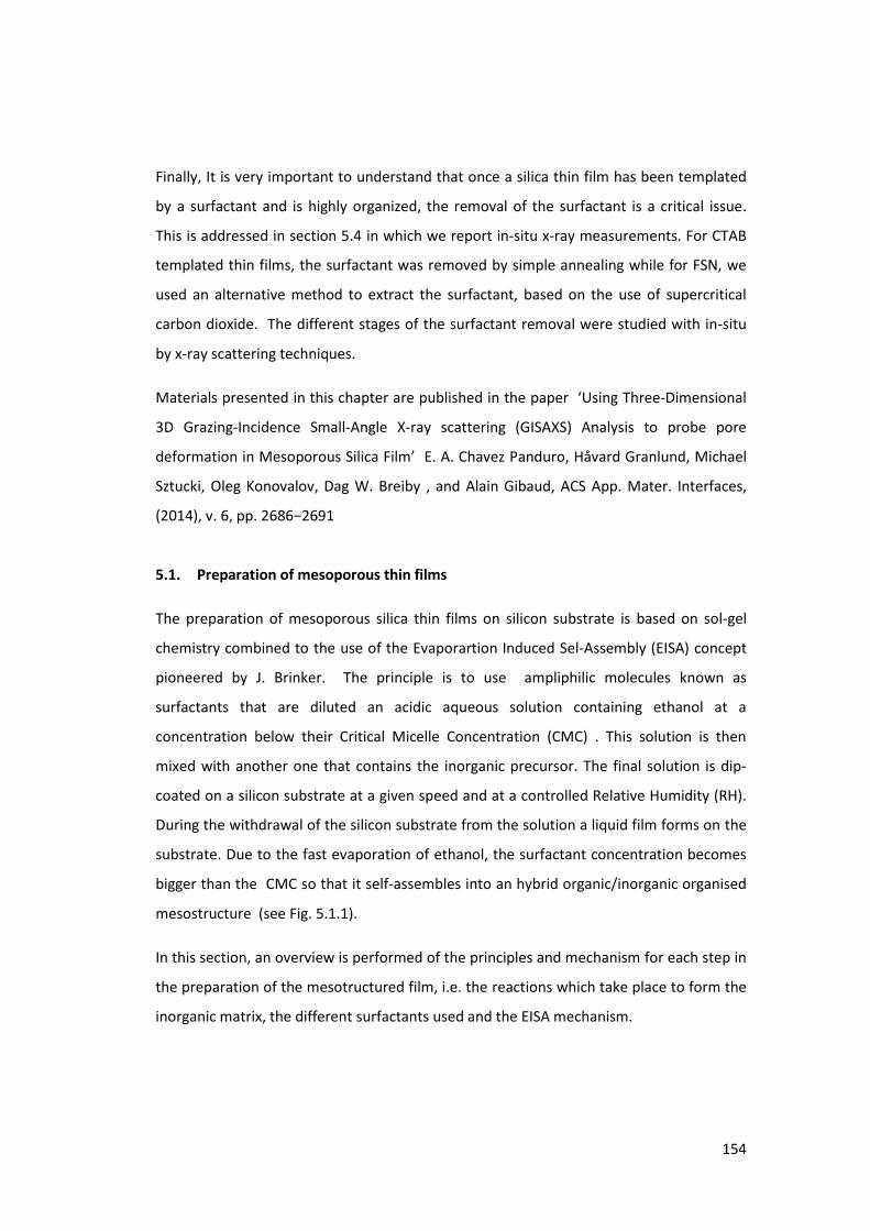
154

Finally, It is very important to understand that once a silica thin film has been templated

by a surfactant and is highly organized, the removal of the surfactant is a critical issue.

This is addressed in section 5.4 in which we report in-situ x-ray measurements. For CTAB

templated thin films, the surfactant was removed by simple annealing while for FSN, we

used an alternative method to extract the surfactant, based on the use of supercritical

carbon dioxide. The different stages of the surfactant removal were studied with in-situ

by x-ray scattering techniques.

Materials presented in this chapter are published in the pape Usi g Th ee-Dimensional

3D Grazing-Incidence Small-Angle X-ray scattering (GISAXS) Analysis to probe pore

defo atio i Mesopo ous “ili a Fil E. A. Cha ez Panduro, Håvard Granlund, Michael

Sztucki, Oleg Konovalov, Dag W. Breiby , and Alain Gibaud, ACS App. Mater. Interfaces,

, . , pp. −

5.1. Preparation of mesoporous thin films

The preparation of mesoporous silica thin films on silicon substrate is based on sol-gel

chemistry combined to the use of the Evaporartion Induced Sel-Assembly (EISA) concept

pioneered by J. Brinker. The principle is to use ampliphilic molecules known as

surfactants that are diluted an acidic aqueous solution containing ethanol at a

concentration below their Critical Micelle Concentration (CMC) . This solution is then

mixed with another one that contains the inorganic precursor. The final solution is dip-

coated on a silicon substrate at a given speed and at a controlled Relative Humidity (RH).

During the withdrawal of the silicon substrate from the solution a liquid film forms on the

substrate. Due to the fast evaporation of ethanol, the surfactant concentration becomes

bigger than the CMC so that it self-assembles into an hybrid organic/inorganic organised

mesostructure (see Fig. 5.1.1).

In this section, an overview is performed of the principles and mechanism for each step in

the preparation of the mesotructured film, i.e. the reactions which take place to form the

inorganic matrix, the different surfactants used and the EISA mechanism.

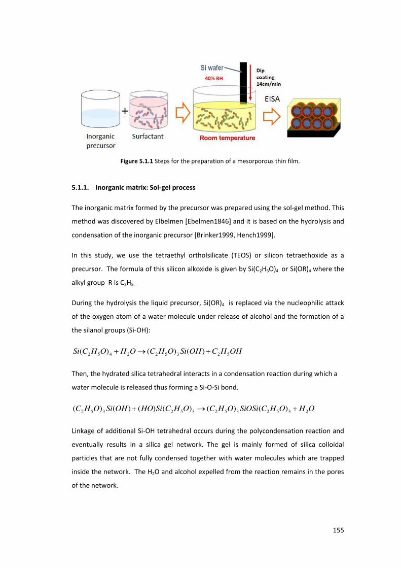
155

Figure 5.1.1 Steps for the preparation of a mesorporous thin film.

5.1.1. Inorganic matrix: Sol-gel process

The inorganic matrix formed by the precursor was prepared using the sol-gel method. This

method was discovered by Elbelmen [Ebelmen1846] and it is based on the hydrolysis and

condensation of the inorganic precursor [Brinker1999, Hench1999].

In this study, we use the tetraethyl ortholsilicate (TEOS) or silicon tetraethoxide as a

precursor. The formula of this silicon alkoxide is given by Si(C2H5O)4 or Si(OR)4 where the

alkyl group R is C2H5.

During the hydrolysis the liquid precursor, Si(OR)4 is replaced via the nucleophilic attack

of the oxygen atom of a water molecule under release of alcohol and the formation of a

the silanol groups (Si-OH):

OHHCOHSiOHCOHOHCSi 523522452 )()()(

Then, the hydrated silica tetrahedral interacts in a condensation reaction during which a

water molecule is released thus forming a Si-O-Si bond.

OHOHCSiOSiOHCOHCSiHOOHSiOHC 2352352352352 )()()()()()(

Linkage of additional Si-OH tetrahedral occurs during the polycondensation reaction and

eventually results in a silica gel network. The gel is mainly formed of silica colloidal

particles that are not fully condensed together with water molecules which are trapped

inside the network. The H2O and alcohol expelled from the reaction remains in the pores

of the network.

156

With time the colloidal particles and condensed silica species link together to become a

three-dimensional network. The physical characteristics of this gel network depend

greatly upon the size of particle and extent of cross-linking prior to gelation [Hench1990].

The existence of residual Si-OH groups allows further condensation reaction and causes

contraction of the gel. This leads to a contraction of the lattice and a release of solvent.

This phenomenon is called "syneresis". The gel is called xerogel when after a period of

aging is dried at low temperature (25-100°C). When the xerogel is then densified by heat

treatments, glasses or ceramics can be formed [Brinker1990].

Finally, it is important to remark that the rates of hydrolysis-condensation reactions can

be controlled by adjusting some of the following reaction conditions:

- precursor type,

- solvent type and pH,

- Concentrations of the various species present in solution.

A precise adjustment of these variables is a key to tuning the size, shape and surface

chemistry of the inorganic polymers therefore allowing a precise control the properties of

the final material [Brinker1990, Pierre1998].

5.1.2. Surfactants

The surfactants are amphiphilic polymers that form micelles at a specific concentration

known as the CMC. These micelles form supramolecular structures that can be cemented

by inorganic molecules. In the preparation of mesoporous materials it is necessary to use

these micelles, which can serve both as a model pattern as well as a support in the

formation of an inorganic matrix.

Depending on the type of surfactant, its concentration and temperature as well as other

variables such as the surfactant/water weight percentage and especially the surfactant/Si

molar ratio, the mesoporous material can adopt different structures as 3D hexagonal,

cubic, lamellar, etc.

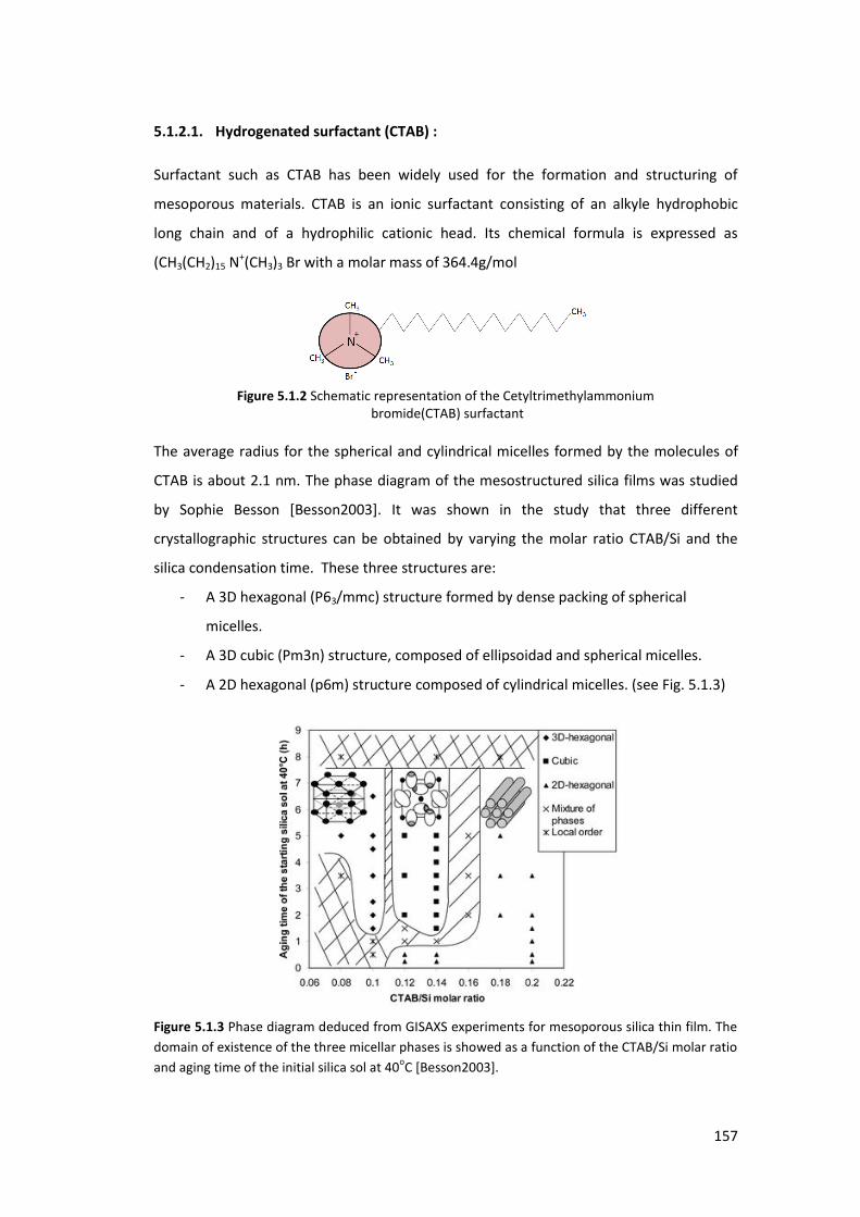
157

5.1.2.1. Hydrogenated surfactant (CTAB) :

Surfactant such as CTAB has been widely used for the formation and structuring of

mesoporous materials. CTAB is an ionic surfactant consisting of an alkyle hydrophobic

long chain and of a hydrophilic cationic head. Its chemical formula is expressed as

(CH3(CH2)15 N+(CH3)3 Br with a molar mass of 364.4g/mol

Figure 5.1.2 Schematic representation of the Cetyltrimethylammonium

bromide(CTAB) surfactant

The average radius for the spherical and cylindrical micelles formed by the molecules of

CTAB is about 2.1 nm. The phase diagram of the mesostructured silica films was studied

by Sophie Besson [Besson2003]. It was shown in the study that three different

crystallographic structures can be obtained by varying the molar ratio CTAB/Si and the

silica condensation time. These three structures are:

- A 3D hexagonal (P63/mmc) structure formed by dense packing of spherical

micelles.

- A 3D cubic (Pm3n) structure, composed of ellipsoidad and spherical micelles.

- A 2D hexagonal (p6m) structure composed of cylindrical micelles. (see Fig. 5.1.3)

Figure 5.1.3 Phase diagram deduced from GISAXS experiments for mesoporous silica thin film. The

domain of existence of the three micellar phases is showed as a function of the CTAB/Si molar ratio

and aging time of the initial silica sol at 40oC [Besson2003].

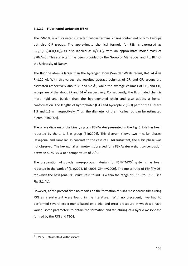
158

5.1.2.2. Fluorinated surfactant (FSN)

The FSN-100 is a fluorinated surfactant whose terminal chains contain not only C-H groups

but also C-F groups. The approximate chemical formula for FSN is expressed as

C8F17C2H4(OCH2CH2)9OH also labeled as R8F(EO)9 with an approximate molar mass of

870g/mol. This surfactant has been provided by the Group of Marie Joe and J.L. Blin of

the University of Nancy.

The fluorine atom is larger than the hydrogen atom (Van der Waals radius, R=1.74 Å vs

R=1.20 Å). With this values, the resulted average volumes of CF2 and CF3 groups are

estimated respectively about 38 and 92 Å3, while the average volumes of CH2 and CH3

groups are of the about 27 and 54 Å3 respectively. Consequently, the fluorinated chain is

more rigid and bulkier than the hydrogenated chain and also adopts a helical

conformation. The lengths of hydrophobic (C-F) and hydrophilic (C-H) part of the FSN are

1.5 and 1.6 nm respectively. Thus, the diameter of the micelles rod can be estimated

6.2nm [Blin2004].

The phase diagram of the binary system FSN/water presented in the Fig. 5.1.4a has been

reported by the J. L. Blin group [Blin2004]. This diagram shows two micellar phases

Hexagonal and Lamellar. In contrast to the case of CTAB surfactant, the cubic phase was

not observed. The hexagonal symmetry is observed for a FSN/water weight concentration

between 50 % -75 % at a temperature of 20oC.

The preparation of powder mesoporous materials for FSN/TMOS2 systems has been

reported in the work of [Blin2004, Blin2005, Zimmy2009]. The molar ratio of FSN/TMOS,

for which the hexagonal 2D structure is found, is within the range of 0.119 to 0.175 (see

Fig. 5.1.4b).

However, at the present time no reports on the formation of silica mesoporous films using

FSN as a surfactant were found in the literature. With no precedent, we had to

performed several experiments based on a trial and error procedure in which we have

varied some parameters to obtain the formation and structuring of a hybrid mesophase

formed by the FSN and TEOS.

2 TMOS : Tetramethyl orthosilicate

159

Figure 5.1.4 a) Phase diagram of the binary system FSN/water. b) Mesoporous materials SAXS

patte s s thesed ith diffe e t su fa ta t/“i ola atio ‘ .

It is worth noting that the substitution of hydrogenated atoms by fluorines ones enhances

the chemical and thermal stability of the surfactant. i.e. a C-F bond energy of 552kJmol-1

instead of 338kJmol-1 for the C-H bond [Kissa1994]. The presence of fluorine atoms also

strongly affects the properties of the surfactants and particularly its hydrophobicity.

The specific solvent-molecular interactions between low dielectric fluids, such as CO2, and

fluorocarbon surfactants can be exploited also for pore expansion of mesostructured silica

e ause the CO2-philic fluorinated tail is readily penetrated by CO2 at high pressure

[Ghosh2008]. The interaction can be expected to be further enhanced when partly

fluorinated surfactants are used, such as those described here, because local dipole

created by the CF2 to CH2 transition induces CO2 quadruple –surfactant interaction.

5.1.3. EISA mechanism

In the preparation of mesostructured films it is necessary that the reactions between the

inorganic matrix (sol-gel) and the formed micelles are properly achieved. In order to

favour this interaction a mechanism known as EISA (Evaporation-Induced Self-Assembly)

has been widely used since it was established in 1997 by Brinker [Brinker1997,

Brinker1999].

This mechanism consists in preparing a very diluted solution containing the precursor, the

surfactant in a volatile solvent in which the surfactant concentration is lower than the

CMC. Then, when the solution is deposited on the substrate via dip-coating or spin-

(a) (b)

160

coating, a very thin silica-surfactant layer will form on the substrate. The drying process

begins as soon as the substrate is withdrawn from the solution. As the film dries, the

evaporation of solvent concentrates the surfactant, silica and other non-volatile species.

The progressive drying increases the surfactant concentration and this drives the self-

assembly of silica-surfactant micelles, which further organize themselves into an

organized silica-surfactant mesostructure [Brinker1999, Grosso2004]. The Figure 5.1.5c

shows schematically the formation of these materials.

Figure 5.1.5 a) Dip-coater designed by A. Gibaud and built by G. Ripault, b) Stages of the dip

coating process b) Schematic diagram of mesoestructure thin film by dip coating. Step1: Initial

solution, where surfactant and silica are mixed homogenously. Step2: Evaporation proceeds and

micelles start to form. Step 3: Evaporation is complete. The film equilibrates with its environment

and the final structure depends on the humidity. Step4: Further inorganic condensation and

stabilisation

5.2. Preparation and Characterization of mesoporous thin films

This section is focused on the description of the methodology used to prepare these films

as well as on their characterization . For the preparation of the CTAB/silica film we briefly

summarize the procedure already reported by [Besson2003] and [Dourdain2006]. For the

preparation of FSN/silica film, several experiments were performed with the aim of

optimizing the methodology to obtain an ordered structure. For the characterization

process of these films, we have used mainly X-ray scattering techniques such as XRR and

GISAXS.

(a)

(b)

(c)

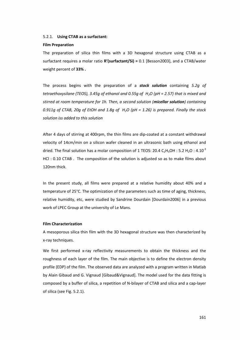
161

5.2.1. Using CTAB as a surfactant:

Film Preparation

The preparation of silica thin films with a 3D hexagonal structure using CTAB as a

surfactant requires a molar ratio ‘ surfacta t/Si = 0.1 [Besson2003], and a CTAB/water

weight percent of 33% .

The process begins with the preparation of a stock solution containing 5.2g of

tetraethoxysilane (TEOS), 3.45g of ethanol and 0.55g of H2O (pH = 2.57) that is mixed and

stirred at room temperature for 1h. Then, a second solution (micellar solution) containing

0.911g of CTAB, 20g of EtOH and 1.8g of H2O (pH = 1.26) is prepared. Finally the stock

solution iss added to this solution

After 4 days of stirring at 400rpm, the thin films are dip-coated at a constant withdrawal

velocity of 14cm/min on a silicon wafer cleaned in an ultrasonic bath using ethanol and

dried. The final solution has a molar composition of 1 TEOS: 20.4 C2H5OH : 5.2 H2O : 4.10-3

HCl : 0.10 CTAB . The composition of the solution is adjusted so as to make films about

120nm thick.

In the present study, all films were prepared at a relative humidity about 40% and a

temperature of 25°C. The optimization of the parameters such as time of aging, thickness,

relative humidity, etc, were studied by Sandrine Dourdain [Dourdain2006] in a previous

work of LPEC Group at the university of Le Mans.

Film Characterization

A mesoporous silica thin film with the 3D hexagonal structure was then characterized by

x-ray techniques.

We first performed x-ray reflectivity measurements to obtain the thickness and the

roughness of each layer of the film. The main objective is to define the electron density

profile (EDP) of the film. The observed data are analyzed with a program written in Matlab

by Alain Gibaud and G. Vignaud [Gibaud&Vignaud]. The model used for the data fitting is

composed by a buffer of silica, a repetition of N-bilayer of CTAB and silica and a cap-layer

of silica (see Fig. 5.2.1).

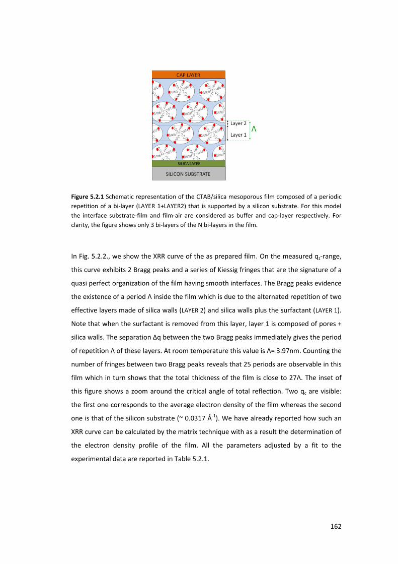
162

Figure 5.2.1 Schematic representation of the CTAB/silica mesoporous film composed of a periodic

repetition of a bi-layer (LAYER 1+LAYER2) that is supported by a silicon substrate. For this model

the interface substrate-film and film-air are considered as buffer and cap-layer respectively. For

clarity, the figure shows only 3 bi-layers of the N bi-layers in the film.

In Fig. 5.2.2., we show the XRR curve of the as prepared film. On the measured qz-range,

this curve exhibits 2 Bragg peaks and a series of Kiessig fringes that are the signature of a

quasi perfect organization of the film having smooth interfaces. The Bragg peaks evidence

the existen e of a pe iod Λ i side the film which is due to the alternated repetition of two

effective layers made of silica walls (LAYER 2) and silica walls plus the surfactant (LAYER 1).

Note that when the surfactant is removed from this layer, layer 1 is composed of pores +

sili a alls. The sepa atio Δ et ee the t o B agg peaks i ediatel gi es the pe iod

of epetitio Λ of these layers. At room te pe atu e this alue is Λ= . 7nm. Counting the

number of fringes between two Bragg peaks reveals that 25 periods are observable in this

fil hi h i tu sho s that the total thi k ess of the fil is lose to Λ. The inset of

this figure shows a zoom around the critical angle of total reflection. Two qc are visible:

the first one corresponds to the average electron density of the film whereas the second

one is that of the silicon substrate (~ 0.0317 Å-1). We have already reported how such an

XRR curve can be calculated by the matrix technique with as a result the determination of

the electron density profile of the film. All the parameters adjusted by a fit to the

experimental data are reported in Table 5.2.1.

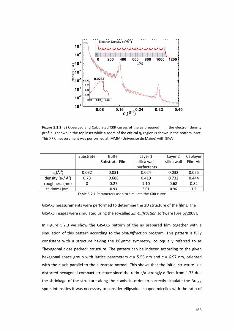
163

0.08 0.16 0.24 0.32 0.4010

-8

10-7

10-6

10-5

10-4

10-3

10-2

10-1

0 200 400 600 800 1000 1200

0.01 0.02 0.03

0.15

0.20

0.25

0.30

Si

Inte

nsity (

u.a

.)

qz(Å

-1)

z(Å)

Electron Density (e-/Å

-3)

0.0261

qz(Å

-1)

Figure 5.2.2 a) Observed and Calculated XRR curves of the as prepared film, the electron density

profile is shown in the top inset while a zoom of the critical qc region is shown in the bottom inset.

This XRR measurement was performed at IMMM (Université du Maine) with 8KeV.

Substrate Buffer Substrate-Film

Layer 1 silica wall

+surfactants

Layer 2 silica wall

Caplayer Film-Air

qc(Å-1) 0.032 0.031 0.024 0.032 0.025

density (e-/ Å3) 0.73 0.688 0.419 0.732 0.444 roughness (nm) 0 0.27 1.10 0.68 0.82

thickness (nm) - 0.93 3.01 0.96 1.5 Table 5.2.1 Parameters used to simulate the XRR curve

GISAXS measurements were performed to determine the 3D structure of the films. The

GISAXS images were simulated using the so-called SimDiffraction software [Breiby2008].

In Figure 5.2.3 we show the GISAXS pattern of the as prepared film together with a

simulation of this pattern according to the SimDiffraction program. This pattern is fully

consistent with a structure having the P63mmc symmetry, colloquially referred to as

he ago al lose pa ked structure. The pattern can be indexed according to the given

hexagonal space group with lattice parameters a = 5.56 nm and c = 6.97 nm, oriented

with the c axis parallel to the substrate normal. This shows that the initial structure is a

distorted hexagonal compact structure since the ratio c/a strongly differs from 1.73 due

the shrinkage of the structure along the c axis. In order to correctly simulate the Bragg

spots intensities it was necessary to consider ellipsoidal shaped micelles with the ratio of

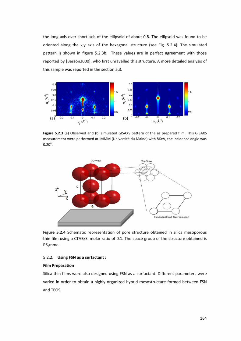
164

the long axis over short axis of the ellipsoid of about 0.8. The ellipsoid was found to be

oriented along the x,y axis of the hexagonal structure (see Fig. 5.2.4). The simulated

pattern is shown in figure 5.2.3b. These values are in perfect agreement with those

reported by [Besson2000], who first unravelled this structure. A more detailed analysis of

this sample was reported in the section 5.3.

Figure 5.2.3 (a) Observed and (b) simulated GISAXS pattern of the as prepared film. This GiSAXS

measurement were performed at IMMM (Université du Maine) with 8KeV, the incidence angle was

0.20o.

Figure 5.2.4 Schematic representation of pore structure obtained in silica mesoporous

thin film using a CTAB/Si molar ratio of 0.1. The space group of the structure obtained is

P63mmc.

5.2.2. Using FSN as a surfactant :

Film Preparation

Silica thin films were also designed using FSN as a surfactant. Different parameters were

varied in order to obtain a highly organized hybrid mesostructure formed between FSN

and TEOS.

qy (Å-1)

qz (

Å-1

)

-0.2 -0.1 0 0.1 0.20

0.05

0.1

0.15

0.2

0.25

0.3

0.5

1

1.5

(a) (b)

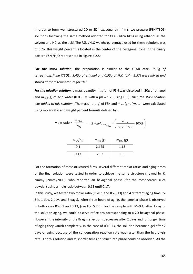
165

In order to form well-structured 2D or 3D hexagonal thin films, we prepare (FSN/TEOS)

solutions following the same method adopted for CTAB silica films using ethanol as the

solvent and HCl as the acid. The FSN /H2O weight percentage used for these solutions was

of 65%, this weight percent is located in the center of the hexagonal zone in the binary

pattern FSN /H2O represented in Figure 5.2.5a.

For the stock solution, the preparation is similar to the CTAB case. 5. g of

tetraethoxysilane (TEOS), 3.45g of ethanol and 0.55g of H2O (pH = 2.57) were mixed and

stirred at room temperature for h.

For the micellar solution, a mass quantity mFSN (g) of FSN was dissolved in 20g of ethanol

and mH20 (g) of acid water (0.055 M with a pH = 1.26 using HCl). Then the stock solution

was added to this solution. The mass mFSN (g) of FSN and mH20 (g) of water were calculated

using molar ratio and weight percent formula defined by:

Mole ratio = Si

FSN

n

n ,

%100%

H2O H2O mm

mweight

FSN

FSNFSN

nFSN/nSi mFSN (g) mH2O (g)

0.1 2.175 1.13

0.13 2.92 1.5

For the formation of mesostructured films, several different molar ratios and aging times

of the final solution were tested in order to achieve the same structure showed by K.

Zimmy [Zimmy2009], who reported an hexagonal phase (for the mesoporous silica

powder) using a mole ratio between 0.11 until 0.17.

In this stud , e tested t o ola atio ‘ = . a d ‘ = . a d diffe e t agi g ti e t=

3 h, 1 day, 2 days and 3 days). After three hours of aging, the lamellar phase is observed

i oth ases ‘ = . a d . , see Fig. . . . Fo the sa ple ith ‘ = . , after 1 day of

the solution aging, we could observe reflexions corresponding to a 2D hexagonal phase.

However, the intensity of the Bragg reflections decreases after 2 days and for longer time

of aging they vanish completely. In the ase of ‘ = . , the solution became a gel after 2

days of aging because of the condensation reaction rate was faster than the hydrolysis

rate. For this solution and at shorter times no structured phase could be observed. All the

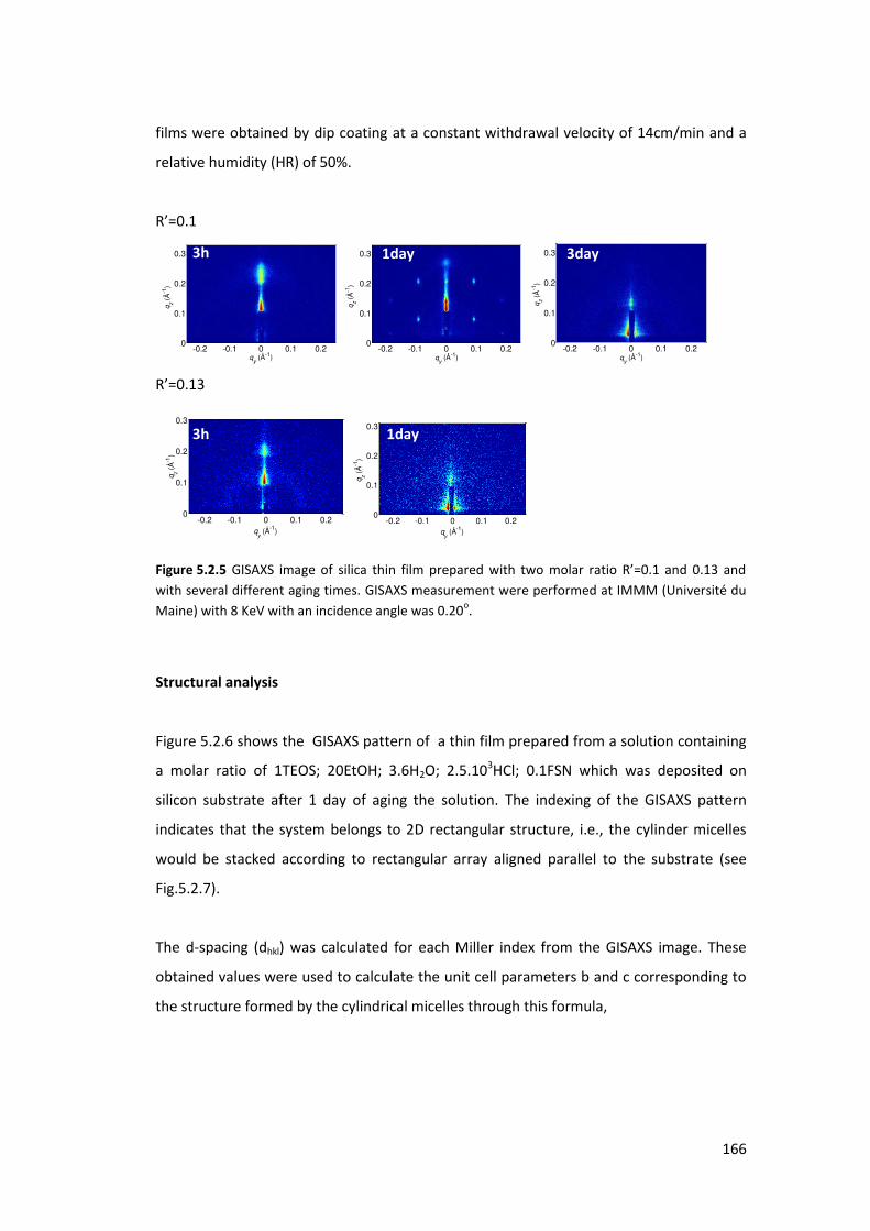
166

films were obtained by dip coating at a constant withdrawal velocity of 14cm/min and a

relative humidity (HR) of 50%.

‘ = .

‘ = .

Figure 5.2.5 GI“AX“ i age of sili a thi fil p epa ed ith t o ola atio ‘ = . a d . a d with several different aging times. GISAXS measurement were performed at IMMM (Université du

Maine) with 8 KeV with an incidence angle was 0.20o.

Structural analysis

Figure 5.2.6 shows the GISAXS pattern of a thin film prepared from a solution containing

a molar ratio of 1TEOS; 20EtOH; 3.6H2O; 2.5.103HCl; 0.1FSN which was deposited on

silicon substrate after 1 day of aging the solution. The indexing of the GISAXS pattern

indicates that the system belongs to 2D rectangular structure, i.e., the cylinder micelles

would be stacked according to rectangular array aligned parallel to the substrate (see

Fig.5.2.7).

The d-spacing (dhkl) was calculated for each Miller index from the GISAXS image. These

obtained values were used to calculate the unit cell parameters b and c corresponding to

the structure formed by the cylindrical micelles through this formula,

qy (Å-1)

qz (

Å-1

)

-0.2 -0.1 0 0.1 0.20

0.1

0.2

0.3

qy (Å-1)

qz (

Å-1

)-0.2 -0.1 0 0.1 0.2

0

0.1

0.2

0.3

qy (Å-1)

qz (

Å-1

)

-0.2 -0.1 0 0.1 0.20

0.1

0.2

0.3

qy (Å-1)

qz (

Å-1

)

-0.2 -0.1 0 0.1 0.20

0.1

0.2

0.3

qy (Å-1)

qz (

Å-1

)

-0.2 -0.1 0 0.1 0.20

0.1

0.2

0.3

3h 1day 3day

3h 1day

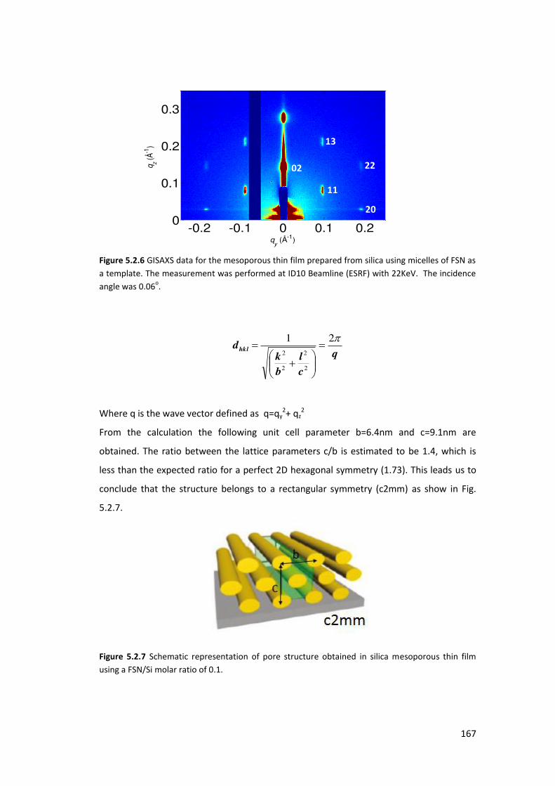
167

Figure 5.2.6 GISAXS data for the mesoporous thin film prepared from silica using micelles of FSN as

a template. The measurement was performed at ID10 Beamline (ESRF) with 22KeV. The incidence

angle was 0.06o.

q

c

l

b

kdhkl

21

2

2

2

2

Where q is the wave vector defined as q=qy2+ qz

2

From the calculation the following unit cell parameter b=6.4nm and c=9.1nm are

obtained. The ratio between the lattice parameters c/b is estimated to be 1.4, which is

less than the expected ratio for a perfect 2D hexagonal symmetry (1.73). This leads us to

conclude that the structure belongs to a rectangular symmetry (c2mm) as show in Fig.

5.2.7.

Figure 5.2.7 Schematic representation of pore structure obtained in silica mesoporous thin film

using a FSN/Si molar ratio of 0.1.

qy (Å-1)

qz (Å

-1)

-0.2 -0.1 0 0.1 0.20

0.1

0.2

0.3

11

13

02

20

22

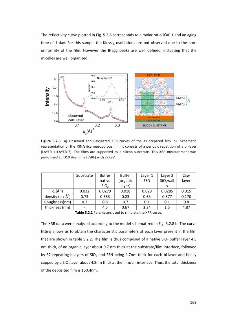
168

The reflectivity curve plotted in Fig. 5.2.8 o espo ds to a ola atio ‘ = . a d a agi g

time of 1 day. For this sample the Kiessig oscillations are not observed due to the non-

uniformity of the film. However the Bragg peaks are well defined, indicating that the

micelles are well organized.

0.1 0.2 0.31E-6

1E-5

1E-4

1E-3

0.01

0.1

0.13 0.140.0

0.2

0.4

0.6

0.8

Inte

nsity

qz(Å

-1)

N= q/q =32

observed

calculated

Inte

nsity

qz(Å)

-1

Figure 5.2.8 a) Observed and Calculated XRR curves of the as prepared film. b) Schematic

representation of the FSN/silica mesoporous film, it consists of a periodic repetition of a bi-layer

(LAYER 1+LAYER 2). The films are supported by a silicon substrate. This XRR measurement was

performed at ID10 Beamline (ESRF) with 22KeV.

Substrate Buffer native SiO2

Buffer (organic

layer)

Layer 1 FSN

Layer 2 SiO2wall

s

Cap- layer

qc(Å

-1) 0.032 0.0279 0.018 0.029 0.0285 0.015

density (e-/ Å3) 0.73 0.553 0.23 0.63 0.577 0.170 Roughness(nm) 0.3 0.8 0.7 0.1 0.1 0.8 thickness (nm) - 4.5 0.67 3.24 1.5 4.87

Table 5.2.2 Parameters used to simulate the XRR curve.

The XRR data were analyzed according to the model schematized in Fig. 5.2.8 b. The curve

fitting allows us to obtain the characteristic parameters of each layer present in the film

that are shown in table 5.2.2. The film is thus composed of a native SiO2 buffer layer 4.5

nm thick, of an organic layer about 0.7 nm thick at the substrate/film interface, followed

by 32 repeating bilayers of SiO2 and FSN being 4.7nm thick for each bi-layer and finally

capped by a SiO2 layer about 4.8nm thick at the film/air interface. Thus, the total thickness

of the deposited film is 160.4nm.

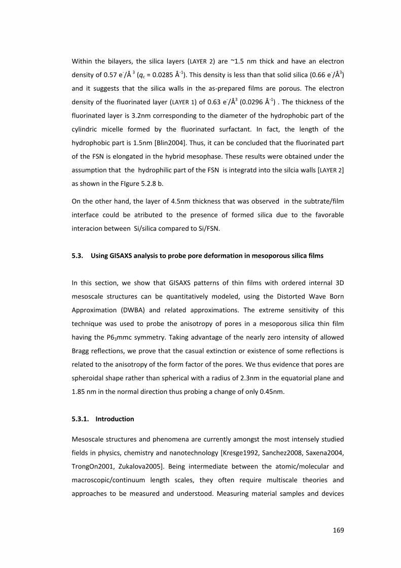
169

Within the bilayers, the silica layers (LAYER 2) are ~1.5 nm thick and have an electron

density of 0.57 e-/Å 3 (qc = 0.0285 Å-1). This density is less than that solid silica (0.66 e-/Å3)

and it suggests that the silica walls in the as-prepared films are porous. The electron

density of the fluorinated layer (LAYER 1) of 0.63 e-/Å3 (0.0296 Å-1) . The thickness of the

fluorinated layer is 3.2nm corresponding to the diameter of the hydrophobic part of the

cylindric micelle formed by the fluorinated surfactant. In fact, the length of the

hydrophobic part is 1.5nm [Blin2004]. Thus, it can be concluded that the fluorinated part

of the FSN is elongated in the hybrid mesophase. These results were obtained under the

assumption that the hydrophilic part of the FSN is integratd into the silcia walls [LAYER 2]

as shown in the FIgure 5.2.8 b.

On the other hand, the layer of 4.5nm thickness that was observed in the subtrate/film

interface could be atributed to the presence of formed silica due to the favorable

interacion between Si/silica compared to Si/FSN.

5.3. Using GISAXS analysis to probe pore deformation in mesoporous silica films

In this section, we show that GISAXS patterns of thin films with ordered internal 3D

mesoscale structures can be quantitatively modeled, using the Distorted Wave Born

Approximation (DWBA) and related approximations. The extreme sensitivity of this

technique was used to probe the anisotropy of pores in a mesoporous silica thin film

having the P63mmc symmetry. Taking advantage of the nearly zero intensity of allowed

Bragg reflections, we prove that the casual extinction or existence of some reflections is

related to the anisotropy of the form factor of the pores. We thus evidence that pores are

spheroidal shape rather than spherical with a radius of 2.3nm in the equatorial plane and

1.85 nm in the normal direction thus probing a change of only 0.45nm.

5.3.1. Introduction

Mesoscale structures and phenomena are currently amongst the most intensely studied

fields in physics, chemistry and nanotechnology [Kresge1992, Sanchez2008, Saxena2004,

TrongOn2001, Zukalova2005]. Being intermediate between the atomic/molecular and

macroscopic/continuum length scales, they often require multiscale theories and

approaches to be measured and understood. Measuring material samples and devices

170

with mesoscale structures is done using both local probes (STM, AFM) and scattering

methods like X-ray powder diffraction and transmission electron microscopy (TEM)

[Zhao1998]. Structural analysis of mesoscale materials processed to thin films is

increasingly carried out by the two surface-sensitive techniques of X-ray reflectivity (XRR)

and GISAXS [Dourdain2005,Gibaud2006], which have the advantage over TEM of not

necessitating sample sectioning that potentially alters the internal structures. In addition,

they are excellently suited for in situ studies, as the highly penetrating nature of X-ray

beams facilitates the use of bulky sample environments [Breivy2013]. XRR provides

quantitative information about the electron density profile in the direction normal to the

surface of the films, by modeling of specular reflectivity data [Dourdain2005, 2008,

Gibaud2003, 2006, Besson2003]. GISAXS, which is essentially SAXS applied to surfaces in

reflection geometry [Besson2000, Doshi2003, Smarsly2005, Grosso2004, Altamura2012,

Buljan2012, Pietra2012] , cf. Fig. 5.3.1, is complementary to XRR, providing information

both in the directions parallel and perpendicular to the thin-film surface, from the diffuse

scattering signal. As the incidence and exit angles involved are small, the usually negligible

effects of refraction and multiple scattering ought to be included for a faithful

quantitative modeling of the scattering data. This is difficult, and in many cases, GISAXS

users report only qualitative structural information. A much studied simplified case is that

of oriented nanoparticles [Renaud2003, Breiby2009] more or less randomly dispersed on

a 2D surface, for which the computer programs isGISAXS [Lazzari2002] or FitGISAXS

[Babonneau2010] are highly adequate. A few researchers [Doshi2003, Smarsly2005,

Grosso2004, Altamura2012, Smilgies2012, Senesi2013, Lee2005, Busch2006, Stein2007]

have tried to extract more quantitative information also from 3D structures in thin films,

however with limited general success because it is quite challenging to analyze the

intensity of Bragg reflections in GISAXS patterns of materials with highly organized porous

structures. It seems fair to state that whereas GISAXS is a relatively easy technique to

apply experimentally, the rather complicated data analysis has impeded GISAXS from

becoming a truly widespread technique.

In this work, we show that GISAXS patterns of thin films with ordered internal 3D

mesoscale structures can be quantitatively modeled, using the Distorted Wave Born

Approximation (DWBA) and related approximations. We go beyond what has previously

been achieved in this field by addressing how the anisotropy of the scattering objects can

be assessed from a complete fit of the data contained in the GISAXS patterns.

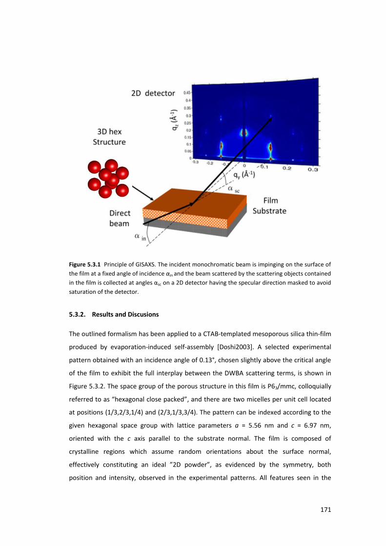
171

Figure 5.3.1 Principle of GISAXS. The incident monochromatic beam is impinging on the surface of

the film at a fixed angle of incidence αin and the beam scattered by the scattering objects contained

i the fil is olle ted at a gles αsc on a 2D detector having the specular direction masked to avoid

saturation of the detector.

5.3.2. Results and Discusions

The outlined formalism has been applied to a CTAB-templated mesoporous silica thin-film

produced by evaporation-induced self-assembly [Doshi2003]. A selected experimental

pattern obtained with an incidence angle of 0.13°, chosen slightly above the critical angle

of the film to exhibit the full interplay between the DWBA scattering terms, is shown in

Figure 5.3.2. The space group of the porous structure in this film is P63/mmc, colloquially

referred to as he ago al close packed , a d the e a e t o i elles pe u it ell lo ated

at positions (1/3,2/3,1/4) and (2/3,1/3,3/4). The pattern can be indexed according to the

given hexagonal space group with lattice parameters a = 5.56 nm and c = 6.97 nm,

oriented with the c axis parallel to the substrate normal. The film is composed of

crystalline regions which assume random orientations about the surface normal,

effe ti el o stituti g a ideal D po de , as e ide ed the s et , oth

position and intensity, observed in the experimental patterns. All features seen in the

172

scattering patterns are accounted for by the presented formalism, where in particular the

doubling of peaks along the qz direction can be explained by the application of the DWBA

formalism, see previous section.

Figure 5.3.2 Experimental GISAXS pattern measured on a mesoporous film in which the CTAB

surfactant was removed, showing the presence of Bragg reflections characteristic of the P63/mmc

structure. White arrows are indicating two specific reflections which are located essentially at the

wave vector transfer with the same modulus. While the 012 reflection is absent, the 110 reflection

is clearly observed although both of them are allowed by the space group.

Most importantly, the 012 reflection allowed by the space group and shown by an

arrow in Figure 5.3.3b does not exist, while the 110 reflection that is located at a similar

wave vector transfer q from the origin is clearly seen. This rather puzzling observation can

be explained by assuming that the pores are not spherical but rather ellipsoidal in shape,

as we shall explain in detail. If a minimum of the form factor function coincides with the

location of a Bragg peak, this peak, even if predicted by the space group symmetry, will

vanish, see Figure 2.5.8. The precision with which one can address the extinction of a

Bragg reflection is related to the fact that the micelles being formed by surfactants are

highly monodisperse so that their form factors exhibit sharp minima, as discussed by Tate

and Hillhouse [Tate2007]. Gratifyingly, we are able to conclusively confirm the slight out-

of-plane compression of the pores previously reported by ellipsometric measurements

[Boissiere2005], relying solely on the GISAXS signal, which opens the path for future in situ

studies of the creation and evolution of the porous networks.

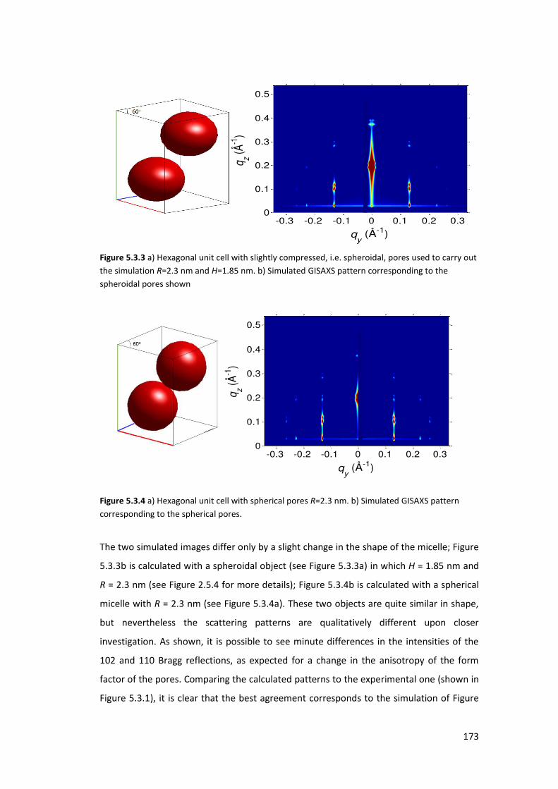
173

Figure 5.3.3 a) Hexagonal unit cell with slightly compressed, i.e. spheroidal, pores used to carry out

the simulation R=2.3 nm and H=1.85 nm. b) Simulated GISAXS pattern corresponding to the

spheroidal pores shown

Figure 5.3.4 a) Hexagonal unit cell with spherical pores R=2.3 nm. b) Simulated GISAXS pattern

corresponding to the spherical pores.

The two simulated images differ only by a slight change in the shape of the micelle; Figure

5.3.3b is calculated with a spheroidal object (see Figure 5.3.3a) in which H = 1.85 nm and

R = 2.3 nm (see Figure 2.5.4 for more details); Figure 5.3.4b is calculated with a spherical

micelle with R = 2.3 nm (see Figure 5.3.4a). These two objects are quite similar in shape,

but nevertheless the scattering patterns are qualitatively different upon closer

investigation. As shown, it is possible to see minute differences in the intensities of the

102 and 110 Bragg reflections, as expected for a change in the anisotropy of the form

factor of the pores. Comparing the calculated patterns to the experimental one (shown in

Figure 5.3.1), it is clear that the best agreement corresponds to the simulation of Figure

qy (Å-1)

qz (Å

-1)

-0.3 -0.2 -0.1 0 0.1 0.2 0.30

0.1

0.2

0.3

0.4

0.5

qy (Å-1)

qz (Å

-1)

-0.3 -0.2 -0.1 0 0.1 0.2 0.30

0.1

0.2

0.3

0.4

0.5

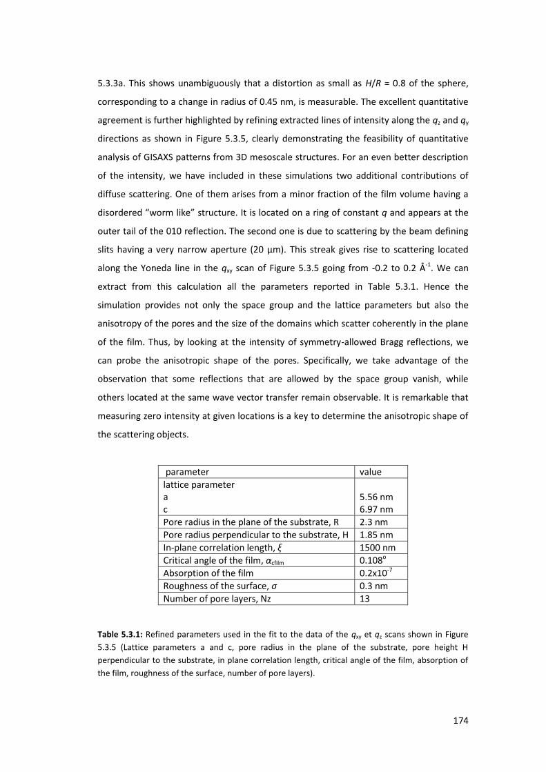
174

5.3.3a. This shows unambiguously that a distortion as small as H/R = 0.8 of the sphere,

corresponding to a change in radius of 0.45 nm, is measurable. The excellent quantitative

agreement is further highlighted by refining extracted lines of intensity along the qz and qy

directions as shown in Figure 5.3.5, clearly demonstrating the feasibility of quantitative

analysis of GISAXS patterns from 3D mesoscale structures. For an even better description

of the intensity, we have included in these simulations two additional contributions of

diffuse scattering. One of them arises from a minor fraction of the film volume having a

diso de ed o like st u tu e. It is lo ated o a i g of o sta t q and appears at the

outer tail of the 010 reflection. The second one is due to scattering by the beam defining

slits having a very narrow aperture (20 µm). This streak gives rise to scattering located

along the Yoneda line in the qxy scan of Figure 5.3.5 going from -0.2 to 0.2 Å-1. We can

extract from this calculation all the parameters reported in Table 5.3.1. Hence the

simulation provides not only the space group and the lattice parameters but also the

anisotropy of the pores and the size of the domains which scatter coherently in the plane

of the film. Thus, by looking at the intensity of symmetry-allowed Bragg reflections, we

can probe the anisotropic shape of the pores. Specifically, we take advantage of the

observation that some reflections that are allowed by the space group vanish, while

others located at the same wave vector transfer remain observable. It is remarkable that

measuring zero intensity at given locations is a key to determine the anisotropic shape of

the scattering objects.

parameter value lattice parameter a c

5.56 nm 6.97 nm

Pore radius in the plane of the substrate, R 2.3 nm Pore radius perpendicular to the substrate, H 1.85 nm In-plane correlation length, ξ 1500 nm Critical angle of the film, αcfilm 0.108o Absorption of the film 0.2x10-7 Roughness of the surface, σ 0.3 nm Number of pore layers, Nz 13

Table 5.3.1: Refined parameters used in the fit to the data of the qxy et qz scans shown in Figure

5.3.5 (Lattice parameters a and c, pore radius in the plane of the substrate, pore height H

perpendicular to the substrate, in plane correlation length, critical angle of the film, absorption of

the film, roughness of the surface, number of pore layers).

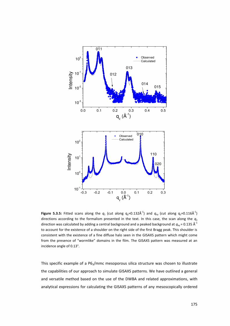
175

0.0 0.1 0.2 0.3 0.4 0.5

10-3

10-2

10-1

100 Observed Calculated

Inte

nsity

qz (Å-1)

011

012

013

014015

-0.3 -0.2 -0.1 0.0 0.1 0.2 0.310

-1

100

101

102

Observed

Calculated

Inte

nsity

qy (Å

-1)

010

110

020

Figure 5.3.5: Fitted scans along the qz (cut along qy=0.132Å-1) and qxy (cut along qz=0.116Å-1)

directions according to the formalism presented in the text. In this case, the scan along the qy

direction was calculated by adding a central background and a peaked background at qxy = 0.135 Å-1

to account for the existence of a shoulder on the right side of the first Bragg peak. This shoulder is

consistent with the existence of a fine diffuse halo seen in the GISAXS pattern which might come

from the prese e of o like do ai s i the fil . The GI“AX“ patte as easu ed at a incidence angle of 0.13°.

This specific example of a P63/mmc mesoporous silica structure was chosen to illustrate

the capabilities of our approach to simulate GISAXS patterns. We have outlined a general

and versatile method based on the use of the DWBA and related approximations, with

analytical expressions for calculating the GISAXS patterns of any mesoscopically ordered

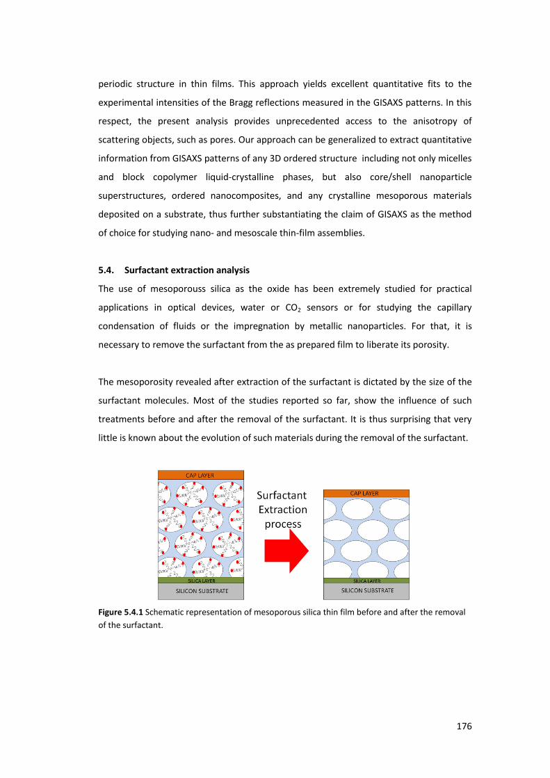
176

periodic structure in thin films. This approach yields excellent quantitative fits to the

experimental intensities of the Bragg reflections measured in the GISAXS patterns. In this

respect, the present analysis provides unprecedented access to the anisotropy of

scattering objects, such as pores. Our approach can be generalized to extract quantitative

information from GISAXS patterns of any 3D ordered structure including not only micelles

and block copolymer liquid-crystalline phases, but also core/shell nanoparticle

superstructures, ordered nanocomposites, and any crystalline mesoporous materials

deposited on a substrate, thus further substantiating the claim of GISAXS as the method

of choice for studying nano- and mesoscale thin-film assemblies.

5.4. Surfactant extraction analysis

The use of mesoporouss silica as the oxide has been extremely studied for practical

applications in optical devices, water or CO2 sensors or for studying the capillary

condensation of fluids or the impregnation by metallic nanoparticles. For that, it is

necessary to remove the surfactant from the as prepared film to liberate its porosity.

The mesoporosity revealed after extraction of the surfactant is dictated by the size of the

surfactant molecules. Most of the studies reported so far, show the influence of such

treatments before and after the removal of the surfactant. It is thus surprising that very

little is known about the evolution of such materials during the removal of the surfactant.

Figure 5.4.1 Schematic representation of mesoporous silica thin film before and after the removal

of the surfactant.

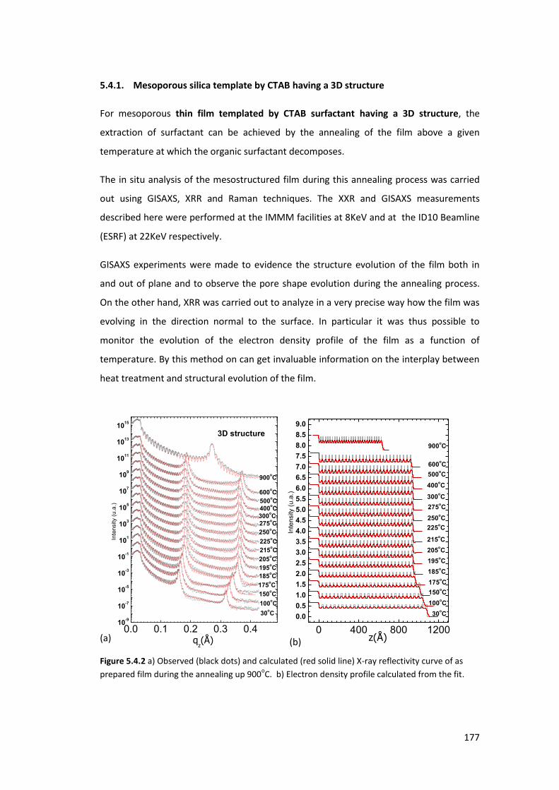
177

5.4.1. Mesoporous silica template by CTAB having a 3D structure

For mesoporous thin film templated by CTAB surfactant having a 3D structure, the

extraction of surfactant can be achieved by the annealing of the film above a given

temperature at which the organic surfactant decomposes.

The in situ analysis of the mesostructured film during this annealing process was carried

out using GISAXS, XRR and Raman techniques. The XXR and GISAXS measurements

described here were performed at the IMMM facilities at 8KeV and at the ID10 Beamline

(ESRF) at 22KeV respectively.

GISAXS experiments were made to evidence the structure evolution of the film both in

and out of plane and to observe the pore shape evolution during the annealing process.

On the other hand, XRR was carried out to analyze in a very precise way how the film was

evolving in the direction normal to the surface. In particular it was thus possible to

monitor the evolution of the electron density profile of the film as a function of

temperature. By this method on can get invaluable information on the interplay between

heat treatment and structural evolution of the film.

0.0 0.1 0.2 0.3 0.410

-9

10-7

10-5

10-3

10-1

101

103

105

107

109

1011

1013

1015

900oC

600oC

500oC

400oC

300oC

275oC

250oC

225oC

215oC

205oC

195oC

185oC

175oC

150oC

100oC

Inte

nsity (

u.a

.)

qz(Å)

30oC

3D structure

0 400 800 1200

0.0

0.5

1.0

1.5

2.0

2.5

3.0

3.5

4.0

4.5

5.0

5.5

6.0

6.5

7.0

7.5

8.0

8.5

9.0

Inte

nsity (

u.a

.)

z(Å)

900oC

600oC

500oC

400oC

300oC

275oC

250oC

225oC

215oC

205oC

195oC

185oC

175oC

150oC

100oC

30oC

Figure 5.4.2 a) Observed (black dots) and calculated (red solid line) X-ray reflectivity curve of as

prepared film during the annealing up 900oC. b) Electron density profile calculated from the fit.

(a) (b)

178

From XRR curves (Figure 5.4.2), it can be seen that the film structure is strongly affected

by the elevation of temperature. At temperatures below 185°C, the film thickness and the

periodic unit length shrink quite significantly as shown by the shift of the Bragg peaks

position towards higher qz values and by the decrease of qz spacing between the Kiessig

fringes while the qc of the film remains constant as the intensity of the Bragg peaks. This is

the evidence that the water molecules contained in the silica gel tend to evaporate

producing the contraction of the silica matrix. The surfactant is not affected by this

treatment since the qc of film remains unchanged as is the contrast of electron density

between the two layers. When the temperature is raised above 180°C, both the position

of the critical qc of the film and the intensity of the Bragg peaks are affected. This shows

that T=180°C is the onset of the removal of the surfactant. When the surfactant is

removed from the film, the contrast of electron density increases between the two layers

and so does the intensity of the Bragg peaks. In addition the electron density of LAYER 1

(i.e. silica walls + surfactant) decreases significantly and so does the critical qc of the film.

The full removal of the surfactant was obtained at a temperature of 250°C (time scale

between each measurements was 4h 20 min). Above this temperature the system is quite

stable up to 500°C. Above 500°C both the film thickness and the periodic unit length

shrink further however the periodic organization of the film along normal, one

dimensional crystal, remains. We were able to follow its behaviour up to 900°C. At this

temperature, GISAXS measurements were performed on the sample confirming that the

3D structure still remains.

Structural evolutions of the film was also monitored by GISAXS. This technique is

particularly useful to correlate the distortion of the micelle aspect ratio (H/R) (Fig. 5.4.5)

with the evolution of the electron density (Fig. 5.4.4) of the mesoporous film obtained by

XRR.

179

-0.3 -0.2 -0.1 0.0 0.1 0.2 0.3

100

101

Observed

Calculated

Inte

nsity

qz(Å

-1)

25oC

0.0 0.1 0.2 0.3

104

105

106

107

108

[013]

observed

calculated

Rela

tive Inte

nsity

qz(Å

-1)

310oC

250oC

210oC

190oC

180oC

170oC

100oC

25oC

[012]

Figure 5.4.3 a) GISAXS pattern corresponding to the mesoporous thin film during the annealing up

to 310oC. b) and c) Fitted scans along qxy (cut at qz=0.116Å-1) and qz (cut at qy=0.132Å-1 ) directions.

The GISAXS patterns were measured at an incidence angle of 0.13°.

From the GISAXS pattern, the change in the pore anisotropy during the annealing process

of the film can be understood by looking at the change in the intensity of the Bragg peaks

(012) and (013) (see Fig. 5.4.3a). In order to calculate the anisotropy a homemade

(a)

(c) (b)

180

program was used that take in account the four scattering terms as well as others

approximations to quantify the distortion of the scattering objects (see section 5.3 for

more details). From the qy direction, we could extract the pore radius in the plane of the

substrate which was found to be R= 22Å. We observe that this radius remains constant

during the process. On the other hand, in the qz direction a clear shift of Bragg peaks is

observed due to the shrinkage of the matrix without affecting the distortion of the micelle

aspect ratio before 180oC. After this temperature, the electron density (Fig. 5.4.4b) and

the micelle distortion (Fig. 5.4.5b) decrease simultaneously until a temperature of 250 oC

is reached. This can be interpreted as the evidence of the micelle disappearance.

200 400 600 800

24

28

32

36

40

(Å

)

IVIIIII

Temperature (°C)

I

200 400 600 800

0.24

0.28

0.32

0.36

0.40

0.44

IVIIIII

elec

tro

n d

ensi

ty (

e/Å

3 )

Temperature (°C)

I

Figure 5.4.4 E olutio of a the thi k ess Λ La e + la e a d the ele t o de sit of the mesoporous film as a function of the temperature. The Parameters were obtained from a fit to the

XRR data.

0 100 200 300

64

68

72

76

I II III

Latt

ice

par

amet

er c

(Å)

Temperature (oC)

0 100 200 300

0.8

0.9

1.0

IIIII

Po

re d

isto

rsio

n (

H/R

)

Temperature (oC)

I

Figure 5.4.5 Evolution of a) the lattice para eter c and b) pore distortion H/R as a function of

temperature. Parameters are obtained after fitting GISAXS data.

The CTAB extraction has been verified through a quasi in-situ analysis using the Raman

spectroscopy technique. For this analysis a small furnace specially adapted to carry out in-

situ measurements was used at the IMMM facilities. During the measurements we

observe a progressive increase of the background (luminescence) as function of

temperature (see Fig. 5.4.6b) that make difficult the in-situ observation of the evolution of

vibration peaks. This luminescence has been attributed to the CTAB degradation during

(a) (b)

(a) (b)

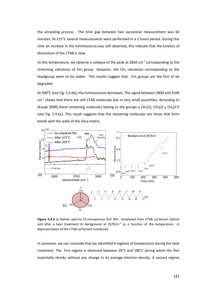
181

the annealing process. The time gap between two successive measurement was 60

minutes. At 215°C several measurements were performed in a 2 hours period. During this

time an increase in the luminescence was still observed, this indicate that the kinetics of

dissolution of the CTAB is slow.

At this temperature, we observe a collapse of the peak at 2850 cm-1 corresponding to the

stretching vibrations of CH2 group. However, the CH3 vibrations corresponding to the

headgroup seem to be stable. This results suggest that, CH2 groups are the first to be

degraded.

At 300oC (see Fig. 5.4.6a), the luminescence decreases. The signal between 2800 and 3100

cm-1 shows that there are still CTAB molecules but in very small quantities. According to

[Kusak 2009] these remaining molecules belong to the groups a CH3(1), CH2(2) y CH3(17)

(see Fig. 5.4.6c). This result suggests that the remaining molecules are those that form

bonds with the walls of the silica matrix.

6

9

12

15

2400 2700 3000

Ra

ma

n I

nte

nsity

As prepared film

After 215oC

After 300oC

2850

N2

CH2

x103

CH3

heagroup

CTAB bulk

wavenumber (cm-1)

0 100 200 300 400 500

0.0

1.7

3.4

5.1

215oC

150oC100

oC

Background at 2670cm-1

Ra

ma

n I

nte

nsity

Time (min)

x103

30oC

175oC

195oC

205oC

Figure 5.4.6 a) Raman spectra of mesoporous thin film templated from CTAB surfactant before

and after a heat treatment b) Background at 2670cm-1 as a function of the temperature c)

Representation of the CTAB surfactant numbered.

In summary, we can conclude that we identified 4 regimes of temperature during the heat

treatment. The first regime is observed between 20°C and 180°C during which the film

essentially shrinks without any change in its average electron density. A second regime

(a) (b)

(c)

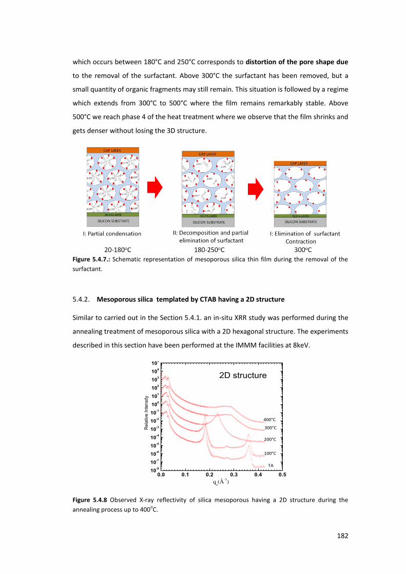
182

which occurs between 180°C and 250°C corresponds to distortion of the pore shape due

to the removal of the surfactant. Above 300°C the surfactant has been removed, but a

small quantity of organic fragments may still remain. This situation is followed by a regime

which extends from 300°C to 500°C where the film remains remarkably stable. Above

500°C we reach phase 4 of the heat treatment where we observe that the film shrinks and

gets denser without losing the 3D structure.

Figure 5.4.7.: Schematic representation of mesoporous silica thin film during the removal of the

surfactant.

5.4.2. Mesoporous silica templated by CTAB having a 2D structure

Similar to carried out in the Section 5.4.1. an in-situ XRR study was performed during the

annealing treatment of mesoporous silica with a 2D hexagonal structure. The experiments

described in this section have been performed at the IMMM facilities at 8keV.

0.0 0.1 0.2 0.3 0.4 0.510

-8

10-7

10-6

10-5

10-4

10-3

10-2

10-1

100

101

102

103

104

105

TA

100°C

200°C

400°C

300°C

Re

lativ

e In

ten

sity

qz(Å-1)

2D structure

Figure 5.4.8 Observed X-ray reflectivity of silica mesoporous having a 2D structure during the

annealing process up to 400oC.

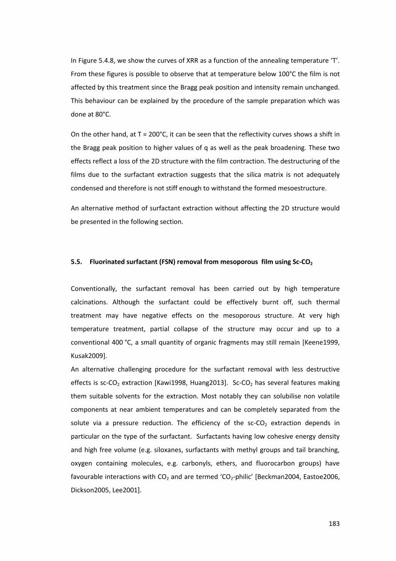
183

In Figure 5.4. , e sho the u es of X‘‘ as a fu tio of the a eali g te pe atu e T .

From these figures is possible to observe that at temperature below 100°C the film is not

affected by this treatment since the Bragg peak position and intensity remain unchanged.

This behaviour can be explained by the procedure of the sample preparation which was

done at 80°C.

On the other hand, at T = 200°C, it can be seen that the reflectivity curves shows a shift in

the Bragg peak position to higher values of q as well as the peak broadening. These two

effects reflect a loss of the 2D structure with the film contraction. The destructuring of the

films due to the surfactant extraction suggests that the silica matrix is not adequately

condensed and therefore is not stiff enough to withstand the formed mesoestructure.

An alternative method of surfactant extraction without affecting the 2D structure would

be presented in the following section.

5.5. Fluorinated surfactant (FSN) removal from mesoporous film using Sc-CO2

Conventionally, the surfactant removal has been carried out by high temperature

calcinations. Although the surfactant could be effectively burnt off, such thermal

treatment may have negative effects on the mesoporous structure. At very high

temperature treatment, partial collapse of the structure may occur and up to a

conventional 400 °C, a small quantity of organic fragments may still remain [Keene1999,

Kusak2009].

An alternative challenging procedure for the surfactant removal with less destructive

effects is sc-CO2 extraction [Kawi1998, Huang2013]. Sc-CO2 has several features making

them suitable solvents for the extraction. Most notably they can solubilise non volatile

components at near ambient temperatures and can be completely separated from the

solute via a pressure reduction. The efficiency of the sc-CO2 extraction depends in

particular on the type of the surfactant. Surfactants having low cohesive energy density

and high free volume (e.g. siloxanes, surfactants with methyl groups and tail branching,

oxygen containing molecules, e.g. carbonyls, ethers, and fluorocarbon groups) have

favourable interactions with CO2 and are termed CO2-phili [Beckman2004, Eastoe2006,

Dickson2005, Lee2001].

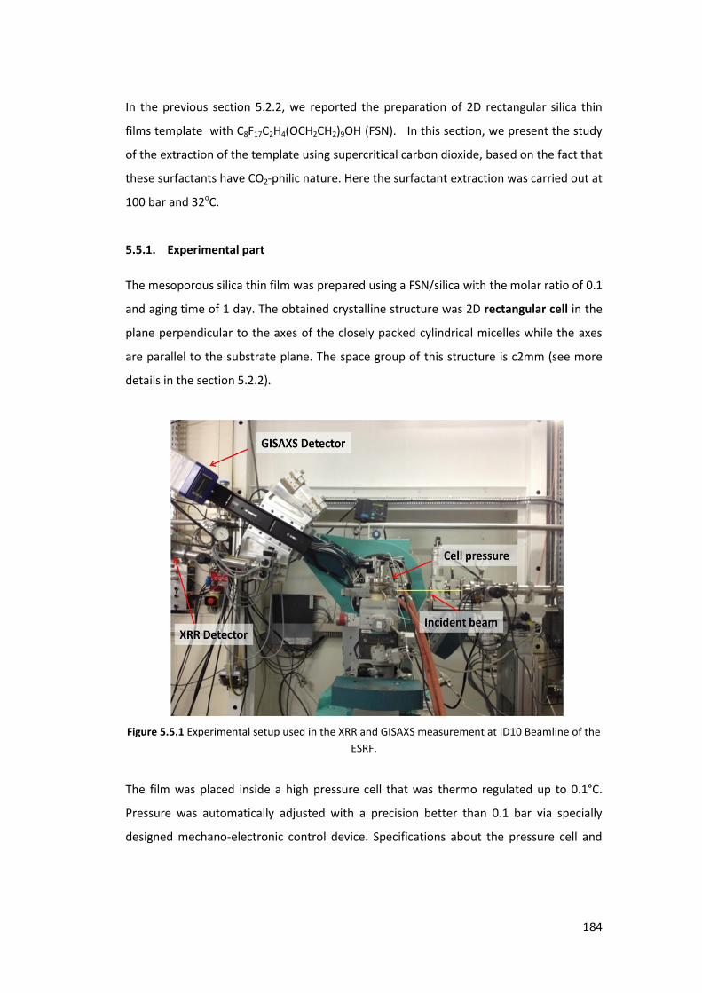
184

In the previous section 5.2.2, we reported the preparation of 2D rectangular silica thin

films template with C8F17C2H4(OCH2CH2)9OH (FSN). In this section, we present the study

of the extraction of the template using supercritical carbon dioxide, based on the fact that

these surfactants have CO2-philic nature. Here the surfactant extraction was carried out at

100 bar and 32oC.

5.5.1. Experimental part

The mesoporous silica thin film was prepared using a FSN/silica with the molar ratio of 0.1

and aging time of 1 day. The obtained crystalline structure was 2D rectangular cell in the

plane perpendicular to the axes of the closely packed cylindrical micelles while the axes

are parallel to the substrate plane. The space group of this structure is c2mm (see more

details in the section 5.2.2).

Figure 5.5.1 Experimental setup used in the XRR and GISAXS measurement at ID10 Beamline of the

ESRF.

The film was placed inside a high pressure cell that was thermo regulated up to 0.1°C.

Pressure was automatically adjusted with a precision better than 0.1 bar via specially

designed mechano-electronic control device. Specifications about the pressure cell and

185

the control device are given in bibliography [Mattenet2010]. All measurements made on

these films were carried out at a constant temperature of 32°C.

XRR experiments were performed at the ID10B beamline of the European Synchrotron

Radiation Facility (ESRF, Grenoble, France) with the monochromatic X-rays beam of 22

keV energy. The high energy X-rays are required to minimise the absorption of the beam

going through the diamond windows of the cell (1 mm) and 35 mm of CO2 in gas and

particularly liquid or sc- state. The time scale between each measurement was 30 min.

The depressurisation process usually took 1h.

5.5.2. Results and Discussion

The experimental results obtained during the pressurisation up to 100 bars are presented

in Fig. 5.5.2. The experiment was carried out on a fresh film which was not yet stabilized.

First, it is noted that XRR curves are not very affected by the elevation of pressure. At the

pressure below 50 bars, a small increase of the thickness (LAYER 1+ LAYER 2) is observed

which is manifested by the shift of the Bragg peak position towards lower qz values. This

result suggests that CO2 penetrates into the micelle causing a slight expansion of the

structure.

0.1 0.2 0.3 0.4

10-6

10-5

10-4

10-3

10-2

10-1

100

101

102

103

0 25 50 75 100175 20045

46

47

48

49

CO2 Pressure (bar)

(Å

)

00

2

4

6

Inte

nsit

y o

f B

rag

g p

eak

Inte

nsi

ty

qz(Å

-1)

100 bar

75 bar

50 bar

25 bar

5 bar

1 bar

1 bar after

Depressurisation

Figure 5.5.2 The evolution of in-situ XRR curves during pressurization of CO2 in the cell. Curves are

translated vertically for clarity. In the top inset, in blue line, the evolutions of the thickness of

(LAYER1+LAYER2) are shown. In the same picture, in red line, we show the evolution of the

intensity of Bragg peak.

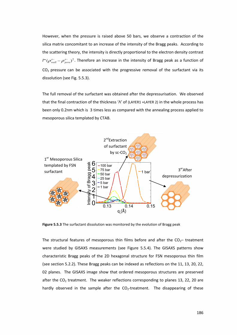
186

However, when the pressure is raised above 50 bars, we observe a contraction of the

silica matrix concomitant to an increase of the intensity of the Bragg peaks. According to

the scattering theory, the intensity is directly proportional to the electron density contrast

I~ 2)( e

pore

e

wall . Therefore an increase in the intensity of Bragg peak as a function of

CO2 pressure can be associated with the progressive removal of the surfactant via its

dissolution (see Fig. 5.5.3).

The full removal of the surfactant was obtained after the depressurisation. We observed

that the final contraction of the thi k ess Λ of (LAYER1 +LAYER 2) in the whole process has

been only 0.2nm which is 3 times less as compared with the annealing process applied to

mesoporous silica templated by CTAB.

Figure 5.5.3 The surfactant dissolution was monitored by the evolution of Bragg peak

The structural features of mesoporous thin films before and after the CO2– treatment

were studied by GISAXS measurements (see Figure 5.5.4). The GISAXS patterns show

characteristic Bragg peaks of the 2D hexagonal structure for FSN mesoporous thin film

(see section 5.2.2). These Bragg peaks can be indexed as reflections on the 11, 13, 20, 22,

02 planes. The GISAXS image show that ordered mesoporous structures are preserved

after the CO2 treatment. The weaker reflections corresponding to planes 13, 22, 20 are

hardly observed in the sample after the CO2-treatment. The disappearing of these

0.13 0.14 0.150123456

1 bar

Inte

nsity o

f B

ragg p

eak

qz(Å)

100 bar

75 bar

50 bar

25 bar

5 bar

1 bar

2ndExtraction

of surfactant

by sc-CO2

1er Mesoporous Silica

templated by FSN

surfactant 3erAfter

depressurization

187

reflections can be assigned to the aspect ratio a distortion of the pores due to the

shrinkage of the sample due to the surfactant removal by sc-CO2.

Figure 5.5.4 GISAXS image of FSN mesoporous thin film before and after the removal of the

surfactant. This GiSAXS measurement was performed at ID10 Beamline (ESRF) with 22KeV. The

incidence angle was 0.06o.

In conclusion, supercritical carbon dioxide extraction is effective extracting the fluorinated

template from the pores of as-prepared mesoporous thin film. The structure of the

mesopore is preserved after the sc-CO2 treatment with a thickness contraction of the

(LAYER1+LAYER2) of 0.2nm.

qy (Å-1)

qz (

Å-1

)

-0.2 -0.1 0 0.1 0.20

0.1

0.2

0.3

qy (Å-1)

qz (

Å-1

)

-0.2 -0.1 0 0.1 0.20

0.1

0.2

0.3

11

13 02

20

22

BEFORE AFTER

188

189

Bibliography

[Altamura2012] Altamura, D.; Holý, V.; Siliqi, D.; Chaitanya Lekshmi, I.; §, Nobile, C.; Maruccio, G.;

Davide Cozzoli, P.; Fan, L.; Gozzo, F.; Giannini, C., Cryst. Growth Des. (2012). , − .

[Babonneau2010] Babonneau, D. J., FitGISAXS: software package for modelling and analysis of

GISAXS data using IGOR Pro. J. Appl. Cryst. (2010) , − .

[Beckman2004] Beckman, E.J. Chem. Commun. (2004) 1885.

[Besson2000] Besson, S.; Gacoin, T.; Jacquiod, C. ; Ricolleau, C.; Babonneau, D,; Boilot, J. P., J.

Mater. Chem. (2000) 10, 1331–1336.

[Besson2003] Besson, S.; Gacoin, T.; Ricolleau, C.; Jacquiod, C. ; Boilot, J. P., J. Mater. Chem. (2003)

13,404.

[Blin2004] Blin, J.L.; Lesieur, P; Stébé, M.J., Langmuir (2004) 20, 491-498.

[Blin2005] Blin, J.L.; Lesieur, P; Stébé, M.J., Microporous and Mesoporous Mater. (2005) 87, 67-76.

[Boissiere2005] Boissière, C.; Grosso, D.; Lepoutre, S.; Nicole, L.; Bruneau, A.B.; Sanchez, C.,

Langmuir (2005) 21 12362.

[Breiby2008] Breiby, D. W.; Bunk, O.; Andreasen, J.; Lemke, H.; Nielsen, M. M. J. Appl. Cryst.

(2008), 41, 262–271.

[Breiby2009] Breiby, D. W.; Chin, P.; Andreasen, J.; Grimsrud, K. A.; Di, Z.; Janssen Rene, A.J.,

Langmuir (2009) 25, 10970-10974.

[Brinker1990] Brinker, C. J.; Hurd, A. J.; Frye, G. C.; Ward, K. J.; Ashley C. S., Journal of Non-

Crystalline Solids (1990) v.121, no.1-3, p.294-302.

[Brinker1997] Lu, Y.; Cangull, R.; Drewlen, C. A.; Anderson, M. T.; Brinker, C. J.; Gong, W.; Guo, Y.;

Soyez, H.; Dunn, B.; Huang M. H.; Zing, J.I., Nature (1997) 389-364.

[Brinker1999] Brinker, C. J.; Lu, Y.; Sellinger, A.; Fan, H., Advanced Materials (1999) 11, 7, p.579.

[Busch2006] Busch, P.; Rauscher, M.; Smilgies, D.; Posselt, D.; Papadakis, C. J. Appl. Crystallogr.

(2006) 39, 433-442.

[Dickson2005] Dickson, J. L.; Smith, P. G.; Dhanuka, V. V.; Srinivasan, V.; Stone, M. T.; Rossky,P. J.;

Behles, J. A.; Keiper, J. S.; Xu, B.; Johnson, C.; DeSimone, J. M.; Johnston, K.P., Ind. Eng. Chem. Res.

(2005) 44, 1370.

[Doshi2003] Doshi, D.A.; Gibaud, A. ; Goletto, V.; Ocko, B.; Brinker, J.J, Am. Chem. Soc. (2003), 125,

11646.

[Dourdain2005] Dourdain S.; Gibaud, A., Appl. Phys. Lett., (2005) 87, 223105.

[Dourdain2006] Dourdain, S., Caracterisation structurale, poreuse et mécanique de films minces de

silice mésoporeuse, PhD thesis, Université du Maine, 2006.

[Dourdain2008] Dourdain, S.; Britton, D. T.; Reichert, H.; Gibaud, A., Appl. Phys. Lett. (2008) 93,

183108.

190

[Eastoe2006] Eastoe, J.; Gold, S.; Steytler, D. C. Langmuir (2006) 22, 9832.

[Ebelmen1846] Ebelmen, J. J., Ann. Chem. Phys. (1846) 57.

[Ghosh2008] Ghosh, K.; Bashadi, S.; Lehmler, H. J.; Rankin, S. E.; Knutson, B. L. Microporous

Mesoporous Mater. (2008) 113, 106-113.

[Gibaud2003] Gibaud, A.; Baptiste, A.; Doshi, D. A.; Brinker, C. J.; Yang, L.; Ocko, B., Europhys. Lett.

(2003)63, 833–839.

[Gibaud2006] Gibaud, A.; Dourdain, S.; Vignaud G., Appl. Surf. Sci., (2006) 253, 1, 3.

[Gibaud&Vignaud] Vignaud, G.; Gibaud, A. Program REFLEX18, a matlab routine for the simulation

of specular x-ray reflectivity data with the matrix technique.

[Grosso2004] Grosso, D.; Cagnol, F.; Soler-Illia, G.J. de A. A.; C epaldi, E. L.; A e its h, H.; B u et-

Bruneau, A.; Bourgeois, A.; Sanchez, C., Adv. Funct. Mater. (2004)14, 309-322.

[Förster2005] Förster, S.; Timmann, A.; Konrad, M.; Schellbach, C.; Meyer, A.; Funari, S.S.;

Mulvaney, P.; Knott, R., J. Phys. Chem. B, (2005) 109, 1347-1360.

[Hench1990] Hench, L. L.; West, J. K., Chem. Rev. (1990) 90. 33-72 93.

[Huang2013] Huang, Z.; Li, J.; Li, H.; Miao, H.; Kawi, S.; Goh, A.H., Separation and Purification

Technology (2013) 118 120–126.

[Kawi1998] Kawi S.; Lai, M. W., Chem. Commun. (1998) 1407-1408.

[Keene1999] Keene, M.T.J.; Gougeon, R.D.M.; Denoyel, R.; Harris, R.K.; Rouquerol, J.; Llewellyn,

P.L.; J. Mater. Chem. (1999) 9 2843–2849.

[Kissa1994] Kissa, E., Fluorinated Surfactants Synthesis properties Applications; Ed.; Surfactant

Science Series 50; Dekker: New York, 1994.

[Kresge1992] Kresge, T.; Leonowicz, M.E.; Roth, W.J.; Vartuli, J.C.; Beck, J.S.; Nature(1992) 359,

710.

[Kusak2009] Goworek, J.; Kierys, A.; Gac, W.; Borówka, A.; Kusak, R., Journal of Thermal Analysis

and Calorimetry (2009) Vol. 96 2, 375–382.

[Lazzari2002] Lazzari, R., J Appl Cryst (2002)35, 406-421.

[Lee2001] Lee, C. T.; Johnston, K. P. Dai, H. J.; Cochran, H. D.; Melnichenko, Y. B.;Wignall, G. D. J.

Phys. Chem. B (2001) 105, 3540.

[Lee2005] Lee B.; Park I.; Yoon J.; Park S.; Kim J.; Kim K.; Chang T.; Ree M. Macromolecules

(2005) 38, 4311-4323.

[Mattenet2010] Mattenet, M.; Lhost, K.; Konovalov, O.; Fall, S.; Pattier, B., An X-Ray

ThermoPressure Cell For Carbon Dioxide AIP Conf. Proc., (2010)1234, 111.

[Pierre1998] Pierre, A. C., I t odu tio to “ol Gel P o essi g , e a edi ió , Klu er Publishers,

1998.

[Pietra2012] Pietra, F.; Rabouw, F. T.; Evers, W. H.; Byelov, D. V.; Petukhov, A. V.; Donegá, C. M.;

Vanmaekelbergh, D., Nano Letters (2012) 12, 5515–5523.

191

[Sanchez2008] Sanchez, C.; Boissière, C. ; Grosso, D. ; Laberty, C. ; Nicole, L., Chem. Mater. (2008)

20, 682–737.

[Smarsly2005] Smarsly, B.; Gibaud, A.; Ruland. W.; Sturmayr, D.; Brinker, C.J., Langmuir (2005) 21,

3858-3866.

[Saxena2004] Saxena, R.; Rodriguez, O.; Cho, W.; Gill, W.N.; Plawsky, J.L.; Baklanov, M.R.;

Mogilkinov, K.P., J. Non Crist. Sol. (2004) 349, 189.

[Senesi2013] Senesi, A.; Eichelsdoerfer, D.; Macfarlane, R.; Jones, M.; Auyeung, E.; Lee, B.;

Mirkin, C., Angew. Chem. Int. Ed. (2013) 52, 6624 –6628.

[Smilgies2012] Smilgies, D.; Heitsch, A.; Korgel, B. J. Phys. Chem. B (2012) , − .

[Stein2007] Stein, G.; Kramer, E.; Li, X.; Wang, J. Macromolecules (2007) 40, 2453-2460.

[Tate2007] Tate, M. P.; Hillhouse, H. W. J. Phys. Chem. C. (2007) , − .

[TrongOn2001] Trong On, D.; Desplantier Giscard, D.; Danumah, C.; Kaliaguine S., Applied Catalysis

A : General (2001) 222, 299-357.

[Zhao1998] Zhao, D.; Feng, J.; Huo, Q.; Melosh, N.; Fredrickson, G. H.; Chmelka, B. F.; Stucky, G.D.,

Science (1998) 279, 548-552.

[Zimmy2009] Zimny, K.; Blin, J.L.; Stébé, M.J., J. Phys. Chem.C (2009) 113, 11285-11293.

[Zukalova2005] Zukalova, M.; Zukal, A.; Kavan, L.; Nazeeruddin, M.K.; Liska, P.; Grätzel,M. Nano

Letters (2005) 5, 9, 1789.

192

193

GENERAL CONCLUSIONS AND PERSPECTIVES

This thesis work has been focused on exploring, by using x-ray techniques available at

synchrotron facilities, the structure of materials exposed to supercritical CO2 under

different pressures. The originality of this work consists in following the evolution of

morphology or the structure of materials during their exposure to this fluid.

The Chapter 3 is concerned to the study of the porosity of CaCO3 microparticles of vaterite

made by a conventional chemical route and by supercritical CO2. It it is shown that this

microspheres exhibit hierarchical porosity made of macropores and mesopores. The

quantitative determination of the pore size and of the pore smoothness was achieved by

implementing the Guinier Porod model recently proposed by Hammouda for two types of

pores. The radii of gyration of the two components and their fractal dimension were

obtained. It was found that macropores have fractal dimension close to 4 indicating

smooth surfaces whereas mesopores located inside the microspheres have smaller fractal

dimension which highlights a rough surface. In both cases radii of gyration are of the

order of 280 nm for the macropores and about 20 times smaller for the mesopores. The

porosity and the surface area was furthermore determined following the approach of for

powders by calculating a Porod invariant based on the effective thickness of the

pulverulent pellet. The specific surface and the mesoporosity are quite close to the results

extracted from N2 adsorption-desorption analysis. This analysis was recently

complemented by CDI experiments at the ID10A beam line of the ESRF. Using the data

acquired from these experiments we were able to reconstruct a 3D image of the complete

shape of these particles and to evidence their inner geometry by 3D tomography. These

types of particles are of great interest for their use as a host matrix for proteins. Thus for

future research, it would become fruitful to carry out a similar 3D image analysis on this

particles after protein encapsulations in order to know the location of these proteins in

the host matrix.

194

Chapter 4 is devoted to the study of ultra thin films of polystyrene under pressurized CO2

conditions. In a first stage, the analysis of AFM images revealed that PS films of 4nm

dewet the surface of HF treated silicon. This was quite surprising as this fact contradicts

theorical expectations. In a second part an in-situ XRR and GISAXS study was conducted

on the swellability as a function of pressure of Polystyrene materials either confined in

one (thin film) and two dimensions (islands). Our results were similar to those reported by

other groups concluding that thin films swell when they are exposed to CO2. However in

the case of PS islands, we observe a much larger swellability than for a homogeneous thin

film. This effect can be attributed to the larger free surface in the island compared with

that of thin films which allows for a greater absorption of CO2. In addition, it was shown

that PS islands (h<10 nm) supported on HF treated silicon do not spread in supercritical

CO2 environment. PS islands remain at a fixed position and grow only in the perpendicular

direction. For future research, it would interesting to study the stability of PS thin film

deposited on native Silicon under CO2 pressure in order to go further on the analysis of

the stability of thin film of Polystyrene. Additionally, the behaviour of such films exposed

to other pressurized gas would be quite instructive.

In Chapter 5, we focused on the analysis of mesoporous silica thin films. These thin films

have been successfully prepared using CTAB and FSN as a surfactant. The CTAB-surfactant

was successfully removed by calcination, a detailed study using XRR and GISAXS identified

various regimes of temperature during the heat treatment. The regime which occurs

between 180°C and 250°C corresponds to the removal of the surfactant accompanied

with a distortion of the pore shape. Above 300°C the surfactant was removed, but it was

found that a small quantity of organic fragments may still remain. After this treatment the

st u tu e does t sh i k up to °C. Fo F“N, a alte ati e ethod of su fa ta t

extraction without affecting the 2D structure have been presented where we show that

supercritical carbon dioxide extraction is effective to extract the fluorinated template

from the pores of as-prepared mesoporous thin film. The structure of the mesopore is

preserved after the sc-CO2 treatment. Finally, we have outlined a general and versatile

method based on the use of the DWBA and related approximations, with analytical

expressions for calculating the GISAXS patterns of any mesoscopically ordered periodic

structure in thin films. This approach yields excellent quantitative fits to the experimental

195

intensities of the Bragg reflections measured in the GISAXS patterns. In this respect, the

present analysis provides unprecedented access to the anisotropy of scattering objects,

such as pores. Our approach can be generalized to extract quantitative information from

GISAXS patterns of any 3D ordered structure including not only micelles and block

copolymer liquid-crystalline phases, but also core/shell nanoparticle superstructures,

ordered nanocomposites, and any crystalline mesoporous materials deposited on a

substrate, thus further substantiating the claim of GISAXS as the method of choice for

studying nano- and mesoscale thin-film assemblies.

196

197

APPENDICES

198

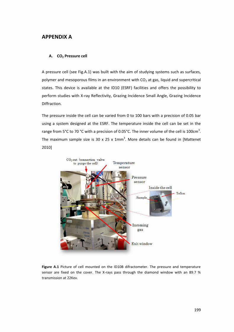
199

APPENDIX A

A. CO2 Pressure cell

A pressure cell (see Fig.A.1) was built with the aim of studying systems such as surfaces,

polymer and mesoporous films in an environment with CO2 at gas, liquid and supercritical

states. This device is available at the ID10 (ESRF) facilities and offers the possibility to

perform studies with X-ray Reflectivity, Grazing Incidence Small Angle, Grazing Incidence

Diffraction.

The pressure inside the cell can be varied from 0 to 100 bars with a precision of 0.05 bar

using a system designed at the ESRF. The temperature inside the cell can be set in the

range from 5°C to 70 °C with a precision of 0.05°C. The inner volume of the cell is 100cm3.

The maximum sample size is 30 x 25 x 1mm3. More details can be found in [Mattenet

2010]

Figure A.1 Picture of cell mounted on the ID10B difractometer. The pressure and temperature

sensor are fixed on the cover. The X-rays pass through the diamond window with an 89.7 %

transmission at 22Kev.

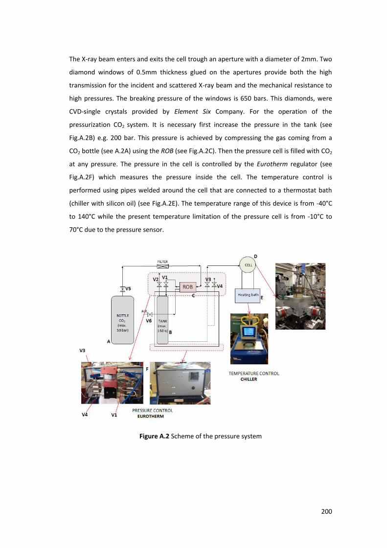
200

The X-ray beam enters and exits the cell trough an aperture with a diameter of 2mm. Two

diamond windows of 0.5mm thickness glued on the apertures provide both the high

transmission for the incident and scattered X-ray beam and the mechanical resistance to

high pressures. The breaking pressure of the windows is 650 bars. This diamonds, were

CVD-single crystals provided by Element Six Company. For the operation of the

pressurization CO2 system. It is necessary first increase the pressure in the tank (see

Fig.A.2B) e.g. 200 bar. This pressure is achieved by compressing the gas coming from a

CO2 bottle (see A.2A) using the ROB (see Fig.A.2C). Then the pressure cell is filled with CO2

at any pressure. The pressure in the cell is controlled by the Eurotherm regulator (see

Fig.A.2F) which measures the pressure inside the cell. The temperature control is

performed using pipes welded around the cell that are connected to a thermostat bath

(chiller with silicon oil) (see Fig.A.2E). The temperature range of this device is from -40°C

to 140°C while the present temperature limitation of the pressure cell is from -10°C to

70°C due to the pressure sensor.

Figure A.2 Scheme of the pressure system

201

A CO2 gas bottle V1 Tank CO2 inlet B Tank of compressed CO2 V2 Tank CO2 outlet C CO2 compressor V3 Cell CO2 inlet D Pressure Cell V4 Cell CO2 outlet E Heating bath V5 CO2 manometer and pressure regulator F Pressure control system V6 Air pressure regulator

Table A.1 General Description of each component

Bibliography

[Mattenet2010] Mattenet, M.; Lhost, K.; Konovalov, O.; Fall, S.; Pattier, B., An X-Ray

ThermoPressure Cell For Carbon Dioxide AIP Conf. Proc., (2010)1234, 111.

202

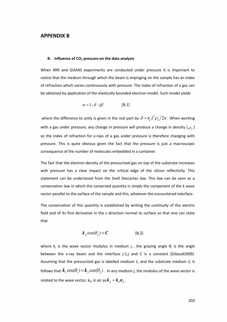
203

APPENDIX B

B. Influence of CO2 pressure on the data analysis

When XRR and GISAXS experiments are conducted under pressure it is important to

notice that the medium through which the beam is impinging on the sample has an index

of refraction which varies continuously with pressure. The index of refraction of a gas can

be obtained by application of the elastically bounded electron model. Such model yields

i--1n [B.1]

where the difference to unity is given in the real part by 22eer . When working

with a gas under pressure, any change in pressure will produce a change in density (e )

so the index of refraction for x-rays of a gas under pressure is therefore changing with

pressure. This is quite obvious given the fact that the pressure is just a macroscopic

consequence of the number of molecules embedded in a container.

The fact that the electron density of the pressurized gas on top of the substrate increases

with pressure has a clear impact on the critical edge of the silicon reflectivity. This

statement can be understood from the Snell Descartes law. This law can be seen as a

conservation law in which the conserved quantity is simply the component of the k wave

vector parallel to the surface of the sample and this, whatever the encountered interface.

The conservation of this quantity is established by writing the continuity of the electric

field and of its first derivative in the z direction normal to surface so that one can state

that

Ck jj )cos( [B.2]

where kj is the a e e to odulus i ediu j , the g azi g a gle θj is the angle

between the x-ray beam and the interface j-1,j and C is a constant [Gibaud2009].

Assuming that the pressurized gas is labelled medium 1, and the substrate medium 2, it

follows that )cos()cos( 2211 kk . In any medium j, the modulus of the wave vector is

related to the wave vector, k0, in air as jj nkk 0 .

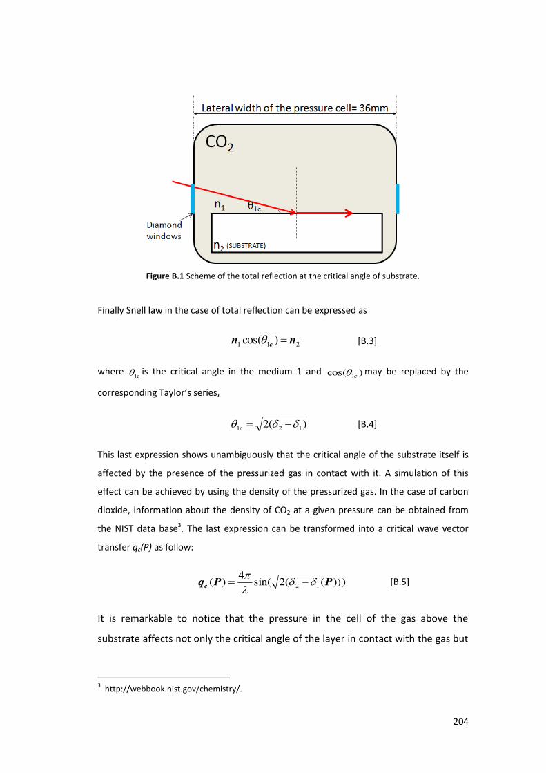
204

Figure B.1 Scheme of the total reflection at the critical angle of substrate.

Finally Snell law in the case of total reflection can be expressed as

211 )cos( nn c [B.3]

where c1 is the critical angle in the medium 1 and )cos( 1c may be replaced by the

o espo di g Ta lo s se ies,

)(2 121 c [B.4]

This last expression shows unambiguously that the critical angle of the substrate itself is

affected by the presence of the pressurized gas in contact with it. A simulation of this

effect can be achieved by using the density of the pressurized gas. In the case of carbon

dioxide, information about the density of CO2 at a given pressure can be obtained from

the NIST data base3. The last expression can be transformed into a critical wave vector

transfer qc(P) as follow:

)))((2sin(4

)( 12 PPqc

[B.5]

It is remarkable to notice that the pressure in the cell of the gas above the

substrate affects not only the critical angle of the layer in contact with the gas but

3 http://webbook.nist.gov/chemistry/.

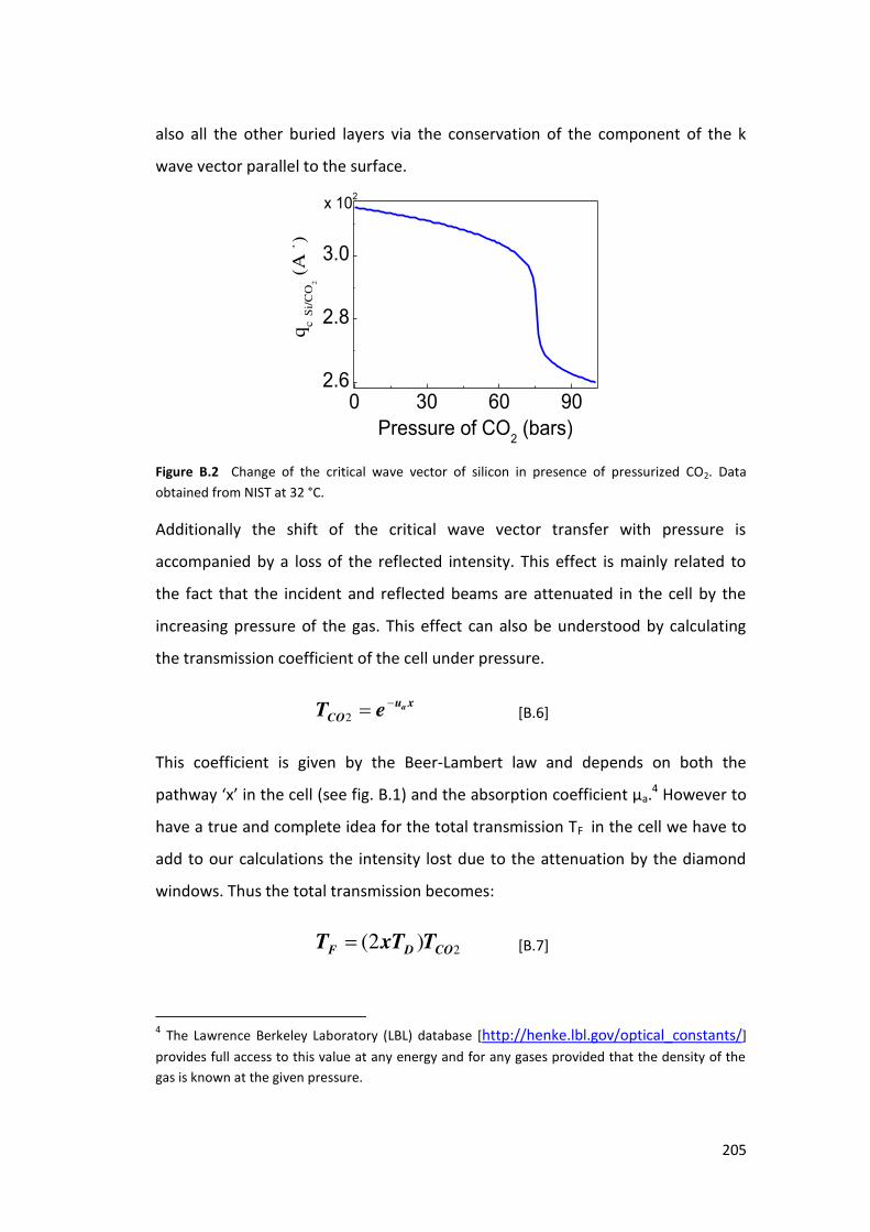
205

also all the other buried layers via the conservation of the component of the k

wave vector parallel to the surface.

0 30 60 902.6

2.8

3.0

q c Si/

CO

2 (Å

-1)

Pressure of CO2 (bars)

x 102

Figure B.2 Change of the critical wave vector of silicon in presence of pressurized CO2. Data

obtained from NIST at 32 °C.

Additionally the shift of the critical wave vector transfer with pressure is

accompanied by a loss of the reflected intensity. This effect is mainly related to

the fact that the incident and reflected beams are attenuated in the cell by the

increasing pressure of the gas. This effect can also be understood by calculating

the transmission coefficient of the cell under pressure.

xu

COaeT

2 [B.6]

This coefficient is given by the Beer-Lambert law and depends on both the

path a i the ell see fig. B.1) and the absorption coefficient µa.4 However to

have a true and complete idea for the total transmission TF in the cell we have to

add to our calculations the intensity lost due to the attenuation by the diamond

windows. Thus the total transmission becomes:

2)2( CODF TxTT [B.7]

4 The Lawrence Berkeley Laboratory (LBL) database [http://henke.lbl.gov/optical_constants/]

provides full access to this value at any energy and for any gases provided that the density of the

gas is known at the given pressure.

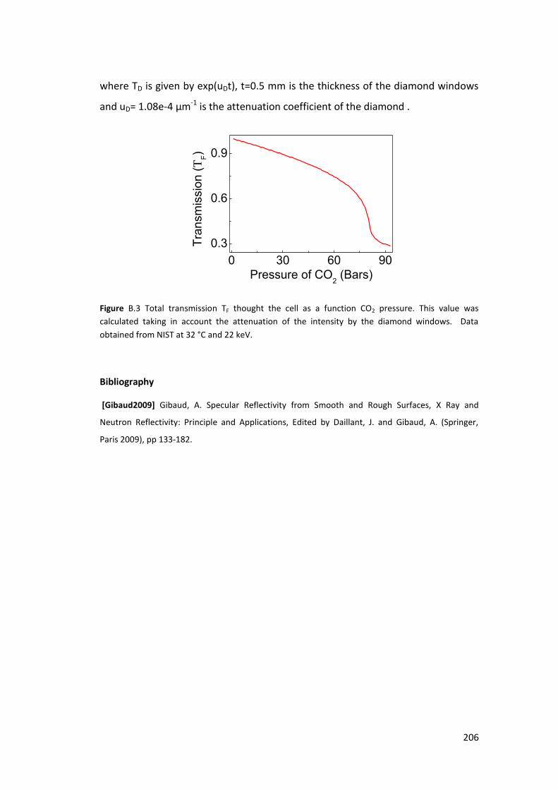
206

where TD is given by exp(uDt), t=0.5 mm is the thickness of the diamond windows

and uD= 1.08e-4 µm-1 is the attenuation coefficient of the diamond .

0 30 60 90

0.3

0.6

0.9

Tra

nsm

issio

n (

TF)

Pressure of CO2 (Bars)

Figure B.3 Total transmission TF thought the cell as a function CO2 pressure. This value was

calculated taking in account the attenuation of the intensity by the diamond windows. Data

obtained from NIST at 32 °C and 22 keV.

Bibliography

[Gibaud2009] Gibaud, A. Specular Reflectivity from Smooth and Rough Surfaces, X Ray and

Neutron Reflectivity: Principle and Applications, Edited by Daillant, J. and Gibaud, A. (Springer,

Paris 2009), pp 133-182.