Synchronous Machines 1.0 Introductionhome.eng.iastate.edu/~jdm/EE456/SynchMachines.pdf1 Synchronous Machines 1.0 Introduction One might easily argue that the synchronous generator

1

Synchronous Machines 1.0 Introduction One might easily argue that the synchronous generator is the most important component in the power system, since synchronous generators • Are the source of 99% of the MW in most

power systems; • Provide frequency regulation and load

following; • Are the main source of voltage control; • Are an important source of oscillation

damping. For that reason, we will spend the remainder of the course studying this component. EE 303 contains a chapter on synchronous generators (Module G1). Sections 2 and 3 of these notes will be basically a review of this module, except that we will more rigorously develop the smooth rotor model used there.

PDF created with pdfFactory trial version www.pdffactory.com

http://www.pdffactory.com

2

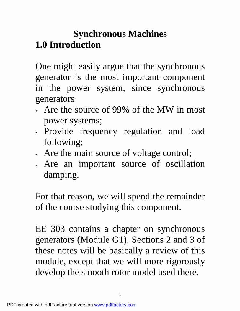
Sections 4 and 5 will extend your knowledge of synchronous generators to account for salient pole machines, 2.0 Synchronous Generator Construction The synchronous generator converts mechanical energy from the turbine into electrical energy. The turbine converts some kind of energy (steam, water, wind) into mechanical energy, as illustrated in Fig. 1 [1].

Fig. 1 [1]



3

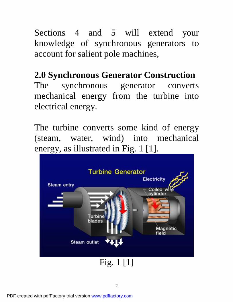
The synchronous generator has two parts: • Stator: carries 3 (3-phase) armature

windings, AC, physically displaced from each other by 120 degrees

• Rotor: carries field windings, connected to an external DC source via slip rings and brushes or to a revolving DC source via a special brushless configuration.

Fig. 2 shows a simplified diagram illustrating the slip-ring connection to the field winding.

Stator

Stator winding Slip

rings

Brushes

Rotor winding

+-

Fig. 2

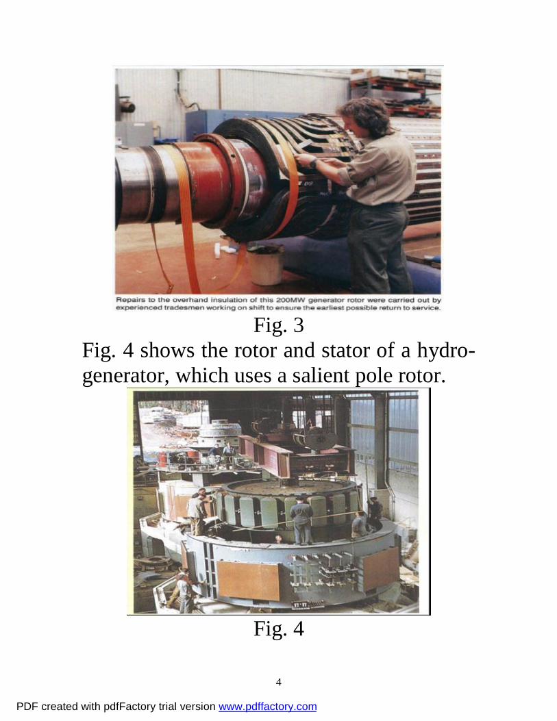
Fig. 3 shows the rotor from a 200 MW steam generator. This is a smooth rotor.



4

Fig. 3

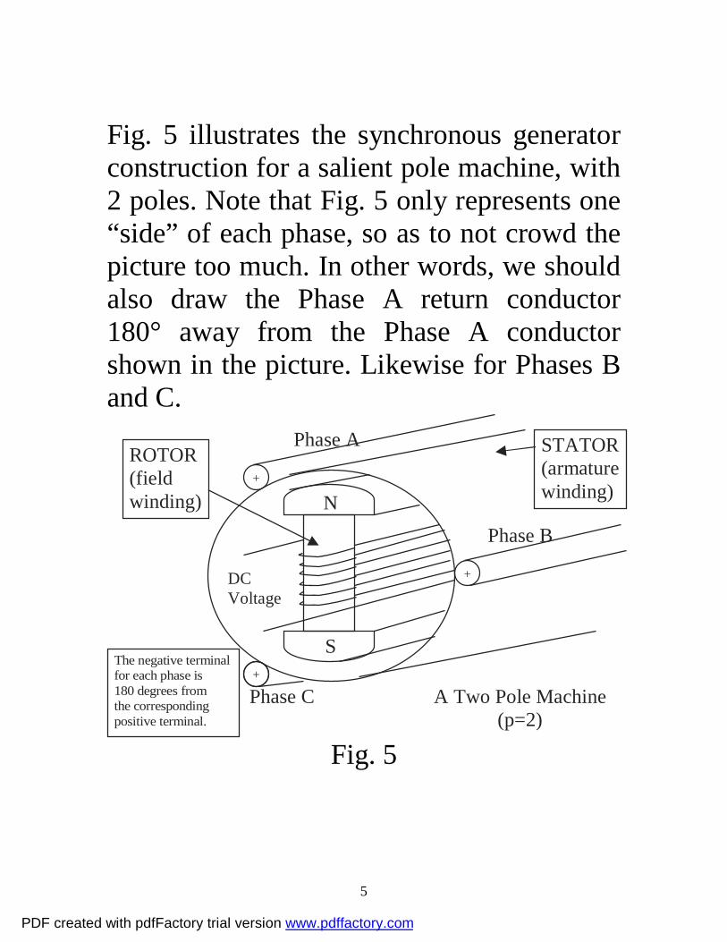
Fig. 4 shows the rotor and stator of a hydro-generator, which uses a salient pole rotor.

Fig. 4



5

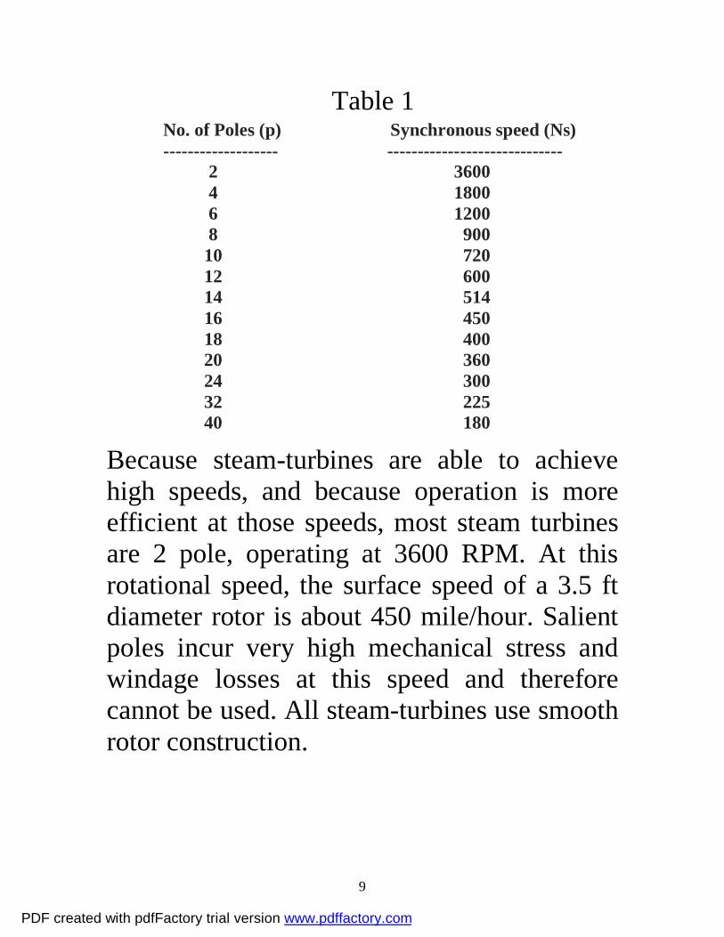
Fig. 5 illustrates the synchronous generator construction for a salient pole machine, with 2 poles. Note that Fig. 5 only represents one “side” of each phase, so as to not crowd the picture too much. In other words, we should also draw the Phase A return conductor 180° away from the Phase A conductor shown in the picture. Likewise for Phases B and C.

A Two Pole Machine (p=2)

Salient Pole Structure

N

S

+

+

DC Voltage

Phase A

Phase B

Phase C

STATOR (armature winding)

ROTOR (field winding)

The negative terminal for each phase is 180 degrees from the corresponding positive terminal.

+

Fig. 5



6

Fig. 6 shows just the rotor and stator (but without stator winding) for a salient pole machine with 4 poles.

A Four Pole Machine (p=4)

(Salient Pole Structure)

N

S

N

S

Fig. 6

The difference between smooth rotor construction and salient pole rotor construction is illustrated in Fig. 7. Note the air-gap in Fig. 7.

Air-gap

Fig. 7



7

The synchronous generator is so-named because it is only at synchronous speed that it functions properly. We will see why later. For now, we define synchronous speed as the speed for which the induced voltage in the armature (stator) windings is synchronized with (has same frequency as) the network voltage. Denote this as ωe. In North America,

ωe=2π(60)= 376.9911≈377rad/sec In Europe,

ωe=2π(50)= 314.1593≈314rad/sec On an airplane,

ωe=2π(400)= 2513.3≈2513rad/sec The mechanical speed of the rotor is related to the synchronous speed through:

( )em pωω

2= (1)

where both ωm and ωe are given in rad/sec. This may be easier to think of if we write

( )mep

ωω2

= (2)



8

Thus we see that, when p=2, we get one electric cycle for every one mechanical cycle. When p=4, we get two electrical cycles for every one mechanical cycle. If we consider that ωe must be constant from one machine to another, then machines with more poles must rotate more slowly than machines with less. It is common to express ωm in RPM, denoted by N; we may easily derive the conversion from analysis of units: Nm=(ωm rad/sec)*(1 rev/2π rad)*(60sec/min) = (30/π)ωm Substitution of ωm=(2/p) ωe=(2/p)2πf=4πf/p

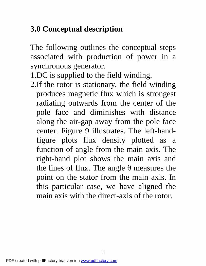
Nm= (30/π)(4πf/p)=120f/p (3) Using (3), we can see variation of Nm with p for f=60 Hz, in Table 1.



9

Table 1

No. of Poles (p) Synchronous speed (Ns) ------------------- ----------------------------- 2 3600 4 1800 6 1200 8 900 10 720 12 600 14 514 16 450 18 400 20 360 24 300 32 225 40 180

Because steam-turbines are able to achieve high speeds, and because operation is more efficient at those speeds, most steam turbines are 2 pole, operating at 3600 RPM. At this rotational speed, the surface speed of a 3.5 ft diameter rotor is about 450 mile/hour. Salient poles incur very high mechanical stress and windage losses at this speed and therefore cannot be used. All steam-turbines use smooth rotor construction.



10

Because hydro-turbines cannot achieve high speeds, they must use a higher number of poles, e.g., 24 and 32 pole hydro-machines are common. But because salient pole construction is less expensive, all hydro-machines use salient pole construction. Fig. 8 illustrates several different constructions for smooth and salient-pole rotors. The red arrows indicate the direction of the flux produced by the field windings.

• Synchronous generator

Rotor construction

Round Rotor Salient Pole

Two pole ωs = 3600 rpm

Four Poleωs = 1800 rpm

Eight Poleωs = 900 rpm

Fig. 8



11

3.0 Conceptual description The following outlines the conceptual steps associated with production of power in a synchronous generator. 1.DC is supplied to the field winding. 2.If the rotor is stationary, the field winding

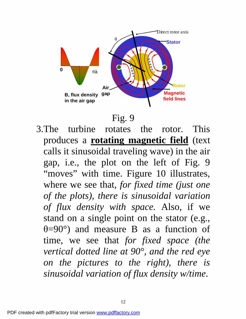
produces magnetic flux which is strongest radiating outwards from the center of the pole face and diminishes with distance along the air-gap away from the pole face center. Figure 9 illustrates. The left-hand-figure plots flux density plotted as a function of angle from the main axis. The right-hand plot shows the main axis and the lines of flux. The angle θ measures the point on the stator from the main axis. In this particular case, we have aligned the main axis with the direct-axis of the rotor.



12

Magneticfield lines

Stator

RotorAirgap

0

B, flux densityin the air gap

θ

θà

Direct rotor axis

Fig. 9

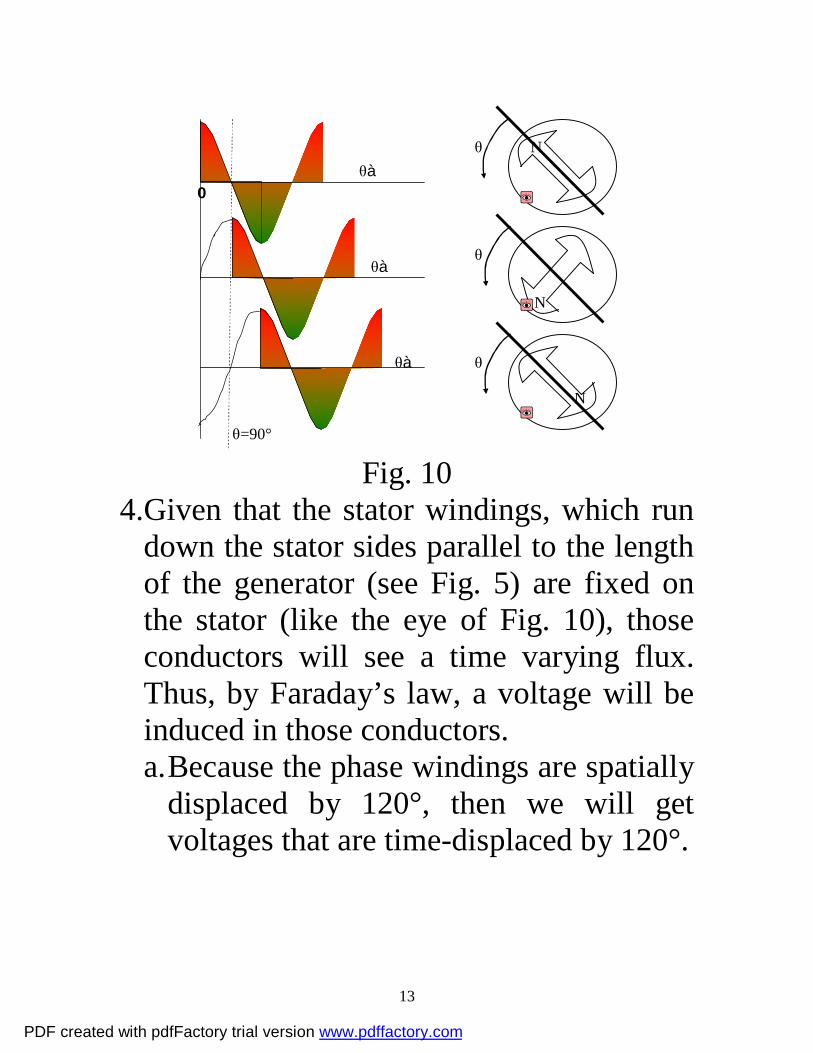
3.The turbine rotates the rotor. This produces a rotating magnetic field (text calls it sinusoidal traveling wave) in the air gap, i.e., the plot on the left of Fig. 9 “moves” with time. Figure 10 illustrates, where we see that, for fixed time (just one of the plots), there is sinusoidal variation of flux density with space. Also, if we stand on a single point on the stator (e.g., θ=90°) and measure B as a function of time, we see that for fixed space (the vertical dotted line at 90°, and the red eye on the pictures to the right), there is sinusoidal variation of flux density w/time.



13

0θà

N

N

N

θ

θ

θ

θà

θà

θ=90° Fig. 10

4.Given that the stator windings, which run down the stator sides parallel to the length of the generator (see Fig. 5) are fixed on the stator (like the eye of Fig. 10), those conductors will see a time varying flux. Thus, by Faraday’s law, a voltage will be induced in those conductors. a. Because the phase windings are spatially

displaced by 120°, then we will get voltages that are time-displaced by 120°.



14

b.If the generator terminals are open-circuited, then the amplitude of the voltages are proportional to

• Speed • Magnetic field strength

And our story ends here if generator terminals are open-circuited.

5.If, however, the phase (armature) windings are connected across a load, then current will flow in each one of them. Each one of these currents will in turn produce a magnetic field. So there will be 4 magnetic fields in the air gap. One from the rotating DC field winding, and one each from the three stationary AC phase windings.

6.The three magnetic fields from the armature windings will each produce flux densities, and the composition of these three flux densities result in a single rotating magnetic field in the air gap.



15

7.This rotating magnetic field from the armature will have the same speed as the rotating magnetic field from the rotor, i.e., these two rotating magnetic fields are in synchronism.

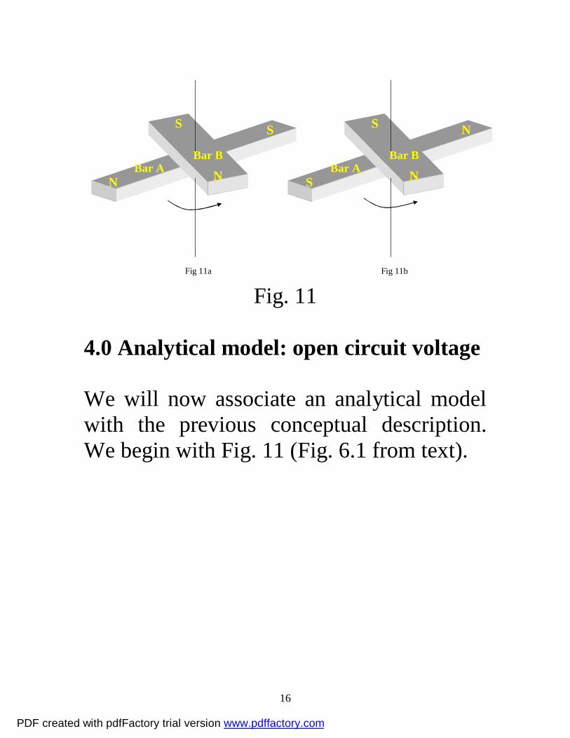
8.The two rotating magnetic fields, that from the rotor and the composite field from the armature, are “locked in,” and as long as they rotate in synchronism, a torque (Torque=P/ωm=Force×radius, where Force is tangential to the rotor surface), is developed. This torque is identical to that which would be developed if two magnetic bars were fixed on the same pivot [2, pg. 171] as shown in Fig 11. In the case of synchronous generator operation, we can think of bar A (the rotor field) as pushing bar B (the armature field), as in Fig. 11a. In the case of synchronous motor operation, we can think of bar B (the armature field) as pulling bar A (the rotor field), as in Fig. 11b.



16

N N

S S

Bar A Bar B

S N

S N

Bar A Bar B

Fig 11a Fig 11b

Fig. 11 4.0 Analytical model: open circuit voltage We will now associate an analytical model with the previous conceptual description. We begin with Fig. 11 (Fig. 6.1 from text).



17

Fig. 11

In this figure, note the following definitions: • θ: the absolute angle between a reference

axis (i.e., fixed point on stator) and the center line of the rotor north pole (direct rotor axis); it is the same as θ of Fig. 9 if, in Fig. 9, we assume that the direct rotor axis is aligned with the reference axis.

• α: the angle made between the reference axis and some point of interest along the air gap circumference.



18

Thus we see that, for any pair of angles θ and α, α-θ gives the angular difference between the centerline of the rotor north pole and the point of interest. We are using two angular measurements in this way in order to address • variation with time as the rotor moves; we

will do this using θ (which gives the rotational position of the centerline of the rotor north pole)

• variation with space for a given θ; we will do this using α (which gives the rotational position of any point on the stator with respect to θ)

We want to describe the flux density, B, in the air gap, due to field current iF only. Assume that maximum air gap flux density, which occurs at the pole center line (α=θ), is Bmax. Assume also that flux density B varies sinusoidally around the air gap (as illustrated in Figs. 9 and 10). Then, for a given θ,



19

)cos()( max θαα −= BB (4) Keep in mind that the flux density expressed by eq. (4) represents only the magnetic field from the winding on the rotor. But, you might say, this is a fictitious situation because the currents in the armature windings will also produce a magnetic field in the air gap, and so we cannot really talk about the magnetic field from the rotor winding alone. We may deal with this issue in an effective and forceful way: assume, for the moment, that the phase A, B, and C armature windings are open, i.e., not connected to the grid or to anything else. Then, currents through them must be zero, and if currents through them are zero, they cannot produce a magnetic field. So we assume that ia=ib=ic=0.



20

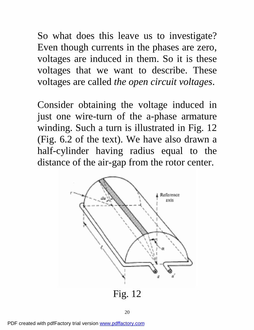
So what does this leave us to investigate? Even though currents in the phases are zero, voltages are induced in them. So it is these voltages that we want to describe. These voltages are called the open circuit voltages. Consider obtaining the voltage induced in just one wire-turn of the a-phase armature winding. Such a turn is illustrated in Fig. 12 (Fig. 6.2 of the text). We have also drawn a half-cylinder having radius equal to the distance of the air-gap from the rotor center.

Fig. 12



21

Note in Fig. 12 that the current direction in the coil is assumed to be from the X-terminal (on the right) to the dot-terminal (on the left). With this current direction, a positive flux direction is established using the right-hand-rule to be upwards. We denote a-phase flux linkages associated with such a directed flux to be λaa’. Our goal, which is to find the voltage induced in this coil of wire, eaa’, can be achieved using Faraday’s Law, which is:

dtd

e aaaa

''

λ−= (5)

So our job at this point is to express the flux linking the a-phase λaa, which comes entirely from the magnetic field produced by the rotor, as a function of time.



22

An aside: The minus sign of eq. (5) expresses Lenz’s Law [3, pp. 27-28], which states that the direction of the voltage in the coil is such that, assuming the coil is the source (as it is when operating as a generator), and the ends are shorted, it will produce current that will cause a flux opposing the original flux change that produced that voltage. Therefore • if flux linkage λaa’ is increasing (originally

positive, meaning upwards through the coil a-a’, and then becoming larger),

• then the current produced by the induced voltage needs to be set up to provide flux linkage in the downward direction of the coil,

• this means the current needs to flow from the terminal a to the terminal a’

• to make this happen across a shorted terminal, the coil would need to be positive at the a’ terminal and negative at the a terminal, as shown in Fig. 13.



23

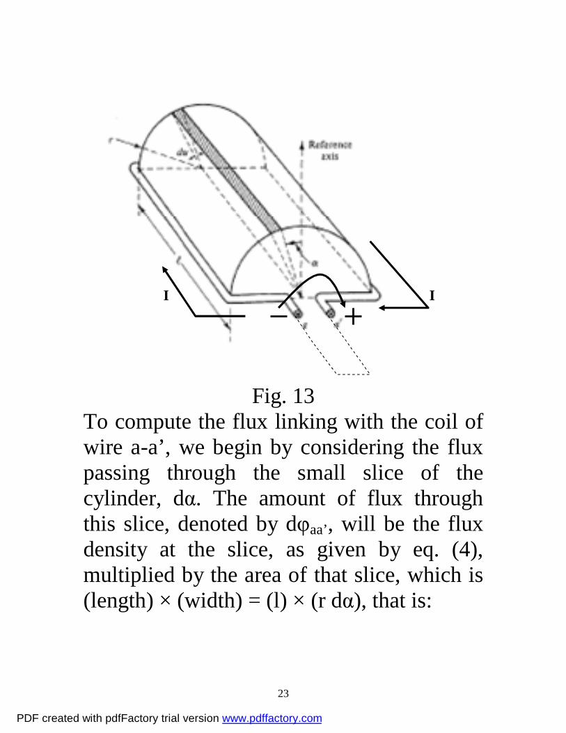
I I

Fig. 13

To compute the flux linking with the coil of wire a-a’, we begin by considering the flux passing through the small slice of the cylinder, dα. The amount of flux through this slice, denoted by dφaa’, will be the flux density at the slice, as given by eq. (4), multiplied by the area of that slice, which is (length) × (width) = (l) × (r dα), that is:



24

αθα

αθαφ

dlrBlrdBd aa

)cos()cos(

max

max'

−=

−= (6)

We can now integrate eq. (6) about the half-cylinder to obtain the flux passing through it (integrating about a full cylinder will give 0, since we would then pick up flux entering and exiting the cylinder).

( ) ( )( )θ

θθ

θπ

θπ

θα

αθαφ

θθ

π

π

π

π

cos2coscos

2sin

2sin

)sin(

)cos(

max

max

coscos

max

2/

2/max

2/

2/max'

lrBlrB

lrB

lrB

dlrBaa

=

−−=

−−−

−=

−=

−=

−

−

−∫

443442143421

(7)

Define φmax=2lrBmax, and we get θϕφ cosmax' =aa (8)

which is the same as eq. (6.2) in the text.



25

Equation (8) indicates that the flux passing through the coil of wire a-a’ depends only on θ. That is, • given the coil of wire is fixed on the

stator, and • given that we know the flux density

occurring in the air gap as a result of the rotor winding,

• we can determine how much of the flux is actually linking with the coil of wire by simply knowing the rotational position of the centerline of the rotor north pole (θ).

But eq. (8) gives us flux, and we need flux linkage. We can get that by just multiplying flux φaa’ by the number of coils of wire N. In the particular case at hand, N=1, but in general, N will be something much higher. Then we obtain:

θϕφλ cosmax'' NN aaaa == (9)



26

Now we need to understand clearly what θ is. It is the centerline of the rotor north pole, BUT, the rotor north pole is rotating! Let’s assume that when the rotor started rotating, it was at θ=θ0, and it is moving at a rotational speed of ω0, then

00 θωθ += t (10) Substitution of eq. (10) into eq. (9) yields:

( )00max' cos θωϕλ += tNaa (11) Now, from eq. (5), we have

( )( )00max'

' cos θωϕλ

+−

=−= tNdt

ddt

de aaaa (12)

We get a –sin from differentiating the cos, and thus we get two negatives, resulting in:

( )000max' sin θωωϕ += tNe aa (13) Define

0maxmax ωϕNE = (14) Then

( )00max' sin θω += tEeaa (15) We can also define the RMS value of eaa’ as



27

2max

'EEaa = (16)

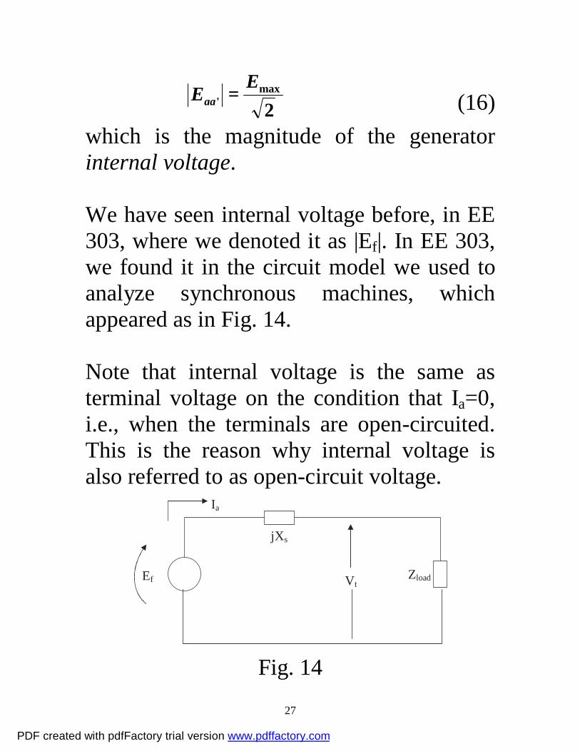
which is the magnitude of the generator internal voltage. We have seen internal voltage before, in EE 303, where we denoted it as |Ef|. In EE 303, we found it in the circuit model we used to analyze synchronous machines, which appeared as in Fig. 14. Note that internal voltage is the same as terminal voltage on the condition that Ia=0, i.e., when the terminals are open-circuited. This is the reason why internal voltage is also referred to as open-circuit voltage.

Ef

jXs

Vt

Ia

Zload

Fig. 14



28

We learned in EE 303 that internal voltage magnitude is proportional to the field current if. This makes sense here, since by eqs. (14) and (16), we see that

220maxmax

'ωϕNEEaa == (17)

and with N and ω0 being machine design parameters (and not parameters that can be adjusted once the machine is built), the only parameter affecting internal voltage is φmax, which is entirely controlled by the current in the field winding, if. One last point here: it is useful at times to have an understanding of the phase relationship between the internal voltage and the flux linkages that produced it. Recall eqs. (11) and (13):

( )00max' cos θωϕλ += tNaa (11) ( )000max' sin θωωϕ += tNe aa (13)

Using sin(x)=cos(x-π/2), we write (13) as: ( )2/cos 000max' πθωωϕ −+= tNeaa (18)



29

Comparing eqs. (11) and (18), we see that the internal voltage lags the flux linkages that produced it by π/2=90° (1/4 turn). This is illustrated by Fig. 15 (same as Fig. E6.1 of Example 6.1). In Fig. 15, the flux linkage phasor is in phase with the direct axis of the rotor.

Reference Axis θ0=π/4

Reference Axis

Flux Linkage Phasor Λaa’

Internal Voltage Phasor Eaa’

a-phase armature winding

Fig. 15 Therefore, the flux linkages phasor is represented by

00'

max' 2

θθφ jaa

jaa eeN

Λ==Λ (19) and then the internal voltage phasor will be



30

( ) ( )2/'

2/0max'

00

2πθπθωφ −− == j

aaj

aa eEeNE (20) Let’s drop the a’ subscript notation from Eaa’, just leaving Ea, so that:

( ) ( )2/2/0max 00

2πθπθωφ −− == j

aj

a eEeNE (21) Likewise, we will get similar expressions for the b- and c-phase internal voltages, according to:

( )3/22/0 ππθ −−= jab eEE (22)

( )3/22/0 ππθ +−= jac eEE (23)

5.0 Armature reaction: one phase winding Armature reaction refers to the influence on the magnetic field in the air gap when the phase windings a, b, and c on the stator are connected across a load.



31

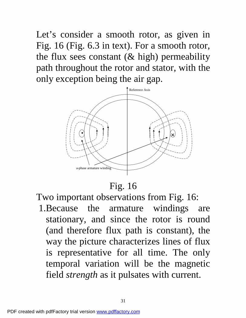
Let’s consider a smooth rotor, as given in Fig. 16 (Fig. 6.3 in text). For a smooth rotor, the flux sees constant (& high) permeability path throughout the rotor and stator, with the only exception being the air gap.

Reference Axis

● ×

a-phase armature winding

Fig. 16 Two important observations from Fig. 16: 1.Because the armature windings are

stationary, and since the rotor is round (and therefore flux path is constant), the way the picture characterizes lines of flux is representative for all time. The only temporal variation will be the magnetic field strength as it pulsates with current.



32

2.The lines of flux made by each side of the a-phase winding will combine in the rotor in such a way so that its maximum strength is along the reference axis, and it varies sinusoidally along the air-gap.

Let’s assume that the current in the a-phase winding is given by:

( )aaa ItIti ∠+= 0cos2)( ω (24) where |Ia| is the RMS current magnitude and

aI∠ is the angle made by the current phasor enabling proper phase relation with its corresponding voltage phasor, eq. (18),

( )2/cos)( 000max πθωωϕ −+= tNtea (18) where 2/0 πθ −=∠ aE . Then the air-gap flux density at the reference axis, where the flux density is maximum, is given by

)()(max, tKitB aa = (25)



33

We emphasize eq. (22) gives flux density at the reference axis only, a fixed point in the air gap corresponding to α=0°. Fig. 17 uses the orange to illustrate what eq. (25) is capturing. The sequence of the 4 pictures, numbered 1,2,3,4, correspond to the sequence-in-time that characterizes flux density seen at the α=0° fixed stator point.

● × ● ×

×

1 2

3 4

● × ●

α=0°

Fig. 17 Because flux minimizes travel in high-reluctance paths, all flux lines are directed radially outwards in the airgap.



34

Substitution of eq. (24) in eq. (25) results in: ( )aaa ItIKtB ∠+= 0max, cos2)( ω (26)

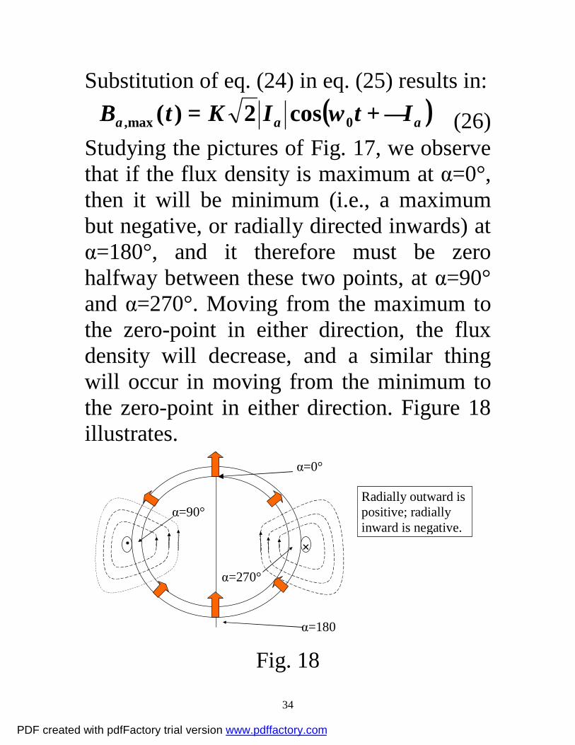
Studying the pictures of Fig. 17, we observe that if the flux density is maximum at α=0°, then it will be minimum (i.e., a maximum but negative, or radially directed inwards) at α=180°, and it therefore must be zero halfway between these two points, at α=90° and α=270°. Moving from the maximum to the zero-point in either direction, the flux density will decrease, and a similar thing will occur in moving from the minimum to the zero-point in either direction. Figure 18 illustrates.

● ×

α=0°

α=180°

α=90°

α=270°

Radially outward is positive; radially inward is negative.

Fig. 18



35

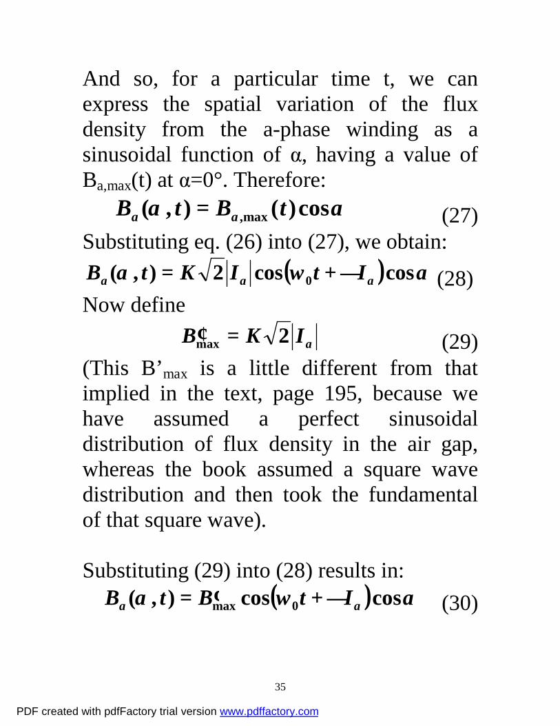
And so, for a particular time t, we can express the spatial variation of the flux density from the a-phase winding as a sinusoidal function of α, having a value of Ba,max(t) at α=0°. Therefore:

αα cos)(),( max, tBtB aa = (27) Substituting eq. (26) into (27), we obtain:

( ) αωα coscos2),( 0 aaa ItIKtB ∠+= (28) Now define

aIKB 2max =′ (29) (This B’max is a little different from that implied in the text, page 195, because we have assumed a perfect sinusoidal distribution of flux density in the air gap, whereas the book assumed a square wave distribution and then took the fundamental of that square wave). Substituting (29) into (28) results in:

( ) αωα coscos),( 0max aa ItBtB ∠+′= (30)



36

Question: Does eq. (30) characterize a rotating magnetic field? To answer this question, we need to recall precisely what we mean by a rotating magnetic field. Let’s re-examine the rotating magnetic field developed by the rotating rotor winding. We expressed this in eq. (4):

)cos()( max θαα −= BB (4) Inserting explicitly the dependence of θ on t:

))(cos(),( max tBtB θαα −= (31) where θ(t)=ω0t+θ0. So there are three attributes: 1.Constant amplitude 2.One sinusoid 3.Argument of sinusoid a function of space

and time Equation (30) has two sinusoids with one being a function of time (first one) and the other being a function of space (second one). And employing trig identities can not result in satisfying the above criteria.



37

Physically, a rotating magnetic field • maintains a constant amplitude waveform

that • continuously moves around the air gap. Equation (30), on the other hand, characterizes a field that • has a time-varying amplitude • which is stationary in the air gap. If you stand at a particular point on the air gap and observe only the field at that point, you will not be able to tell the difference between the two. However, if you cut the stator and spread out the air gap linearly, and observe the entire waveform of both fields, you will find: • the rotating magnetic field moves. • the other one pulsates.



38

A good way to think about this is to consider that in the case of the rotating magnetic field, the flux density is never 0 everywhere in the air gap.WS In contrast, every time the current in the a-phase winding goes to zero, the flux density of the eq. (30) pulsating field goes to zero everywhere in the air gap. Cool. 6.0 Armature reaction: all phase windings We can go through a similar thought process to obtain the flux density produced by the b- and c-phase armature windings. The result will be identical to eq. (30), except that • the time-dependent term will be phase-

shifted consistent with the phase-shifts of the current, and

• the space-dependent term will be phase-shifted consistent with the phase-shifts of the physical windings.



39

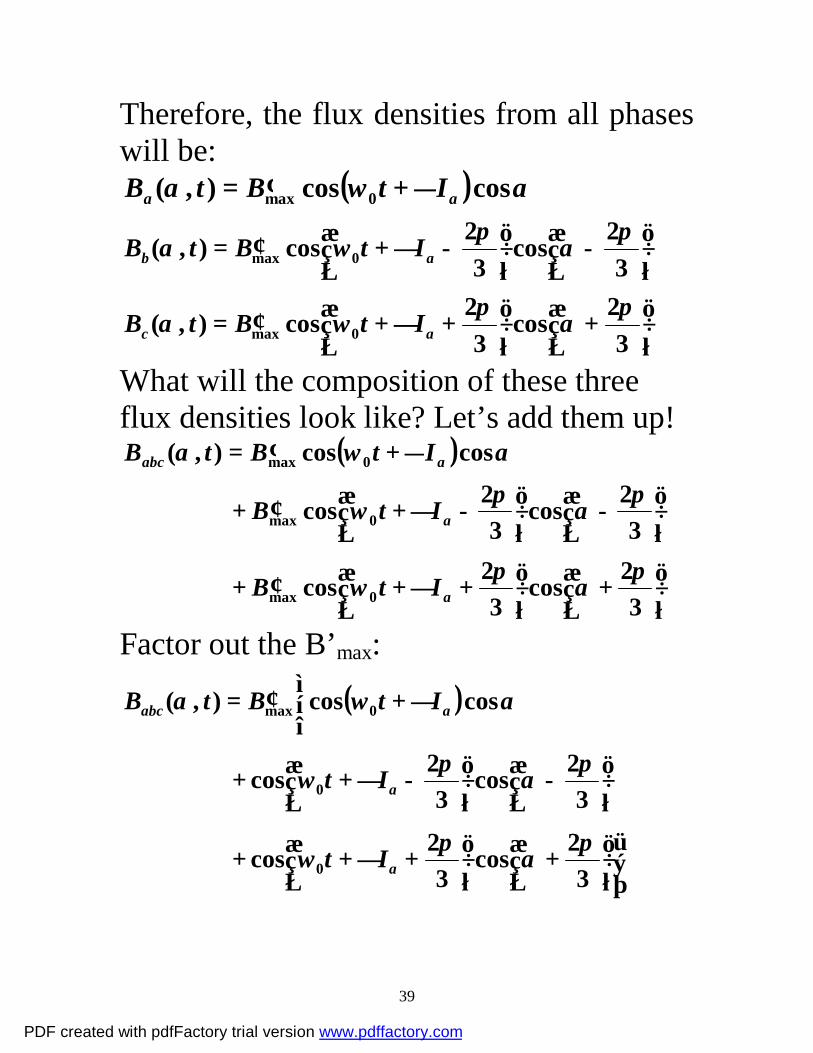
Therefore, the flux densities from all phases will be:

( ) αωα coscos),( 0max aa ItBtB ∠+′=

−

−∠+′=

32cos

32cos),( 0max

πα

πωα ab ItBtB

+

+∠+′=

32cos

32cos),( 0max

πα

πωα ac ItBtB

What will the composition of these three flux densities look like? Let’s add them up!

( )

+

+∠+′+

−

−∠+′+

∠+′=

32cos

32cos

32cos

32cos

coscos),(

0max

0max

0max

πα

πω

πα

πω

αωα

a

a

aabc

ItB

ItB

ItBtB

Factor out the B’max:

( )

+

+∠++

−

−∠++

∠+′=

32cos

32cos

32cos

32cos

coscos),(

0

0

0max

πα

πω

πα

πω

αωα

a

a

aabc

It

It

ItBtB



40

Now deploy the trig identity

[ ])cos()cos(21coscos bababa ++−=

to all three terms. ( ) ( )

+++∠++

−−+∠++

−+−∠++

+−−∠++

+∠++−∠+′

=

32

32cos

32

32cos

32

32cos

32

32cos

coscos2

),(

00

00

00max

πα

πω

πα

πω

πα

πω

πα

πω

αωαωα

aa

aa

aaabc

ItIt

ItIt

ItItBtB

Combine all of the terms with π. ( ) ( )

( )

( )

++∠++−∠++

−+∠++−∠++

+∠++−∠+′

=

34coscos

34coscos

coscos2

),(

00

00

00max

παωαω

παωαω

αωαωα

aa

aa

aaabc

ItIt

ItIt

ItItBtB

Now we notice a very interesting thing. The three cos terms on the right side of each row constitute a balanced set (equal-magnitude terms 120° out of phase). They therefore add to zero! So we have

( ){( )( )}αω

αω

αωα

−∠++

−∠++

−∠+′

=

a

a

aabc

ItIt

ItBtB

0

0

0max

coscos

cos2

),(



41

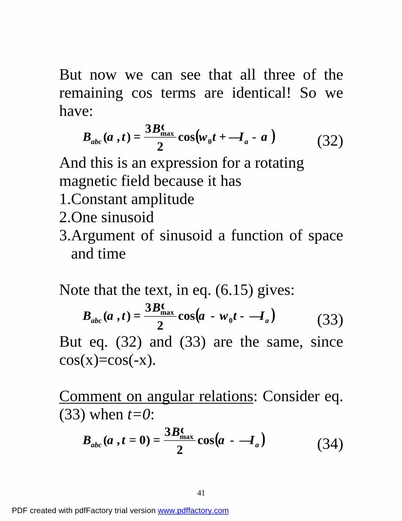
But now we can see that all three of the remaining cos terms are identical! So we have:

( )αωα −∠+′

= aabc ItBtB 0max cos

23),( (32)

And this is an expression for a rotating magnetic field because it has 1.Constant amplitude 2.One sinusoid 3.Argument of sinusoid a function of space

and time Note that the text, in eq. (6.15) gives:

( )aabc ItBtB ∠−−′

= 0max cos

23),( ωαα (33)

But eq. (32) and (33) are the same, since cos(x)=cos(-x). Comment on angular relations: Consider eq. (33) when t=0:

( )aabc IBtB ∠−′

== αα cos2

3)0,( max (34)



42

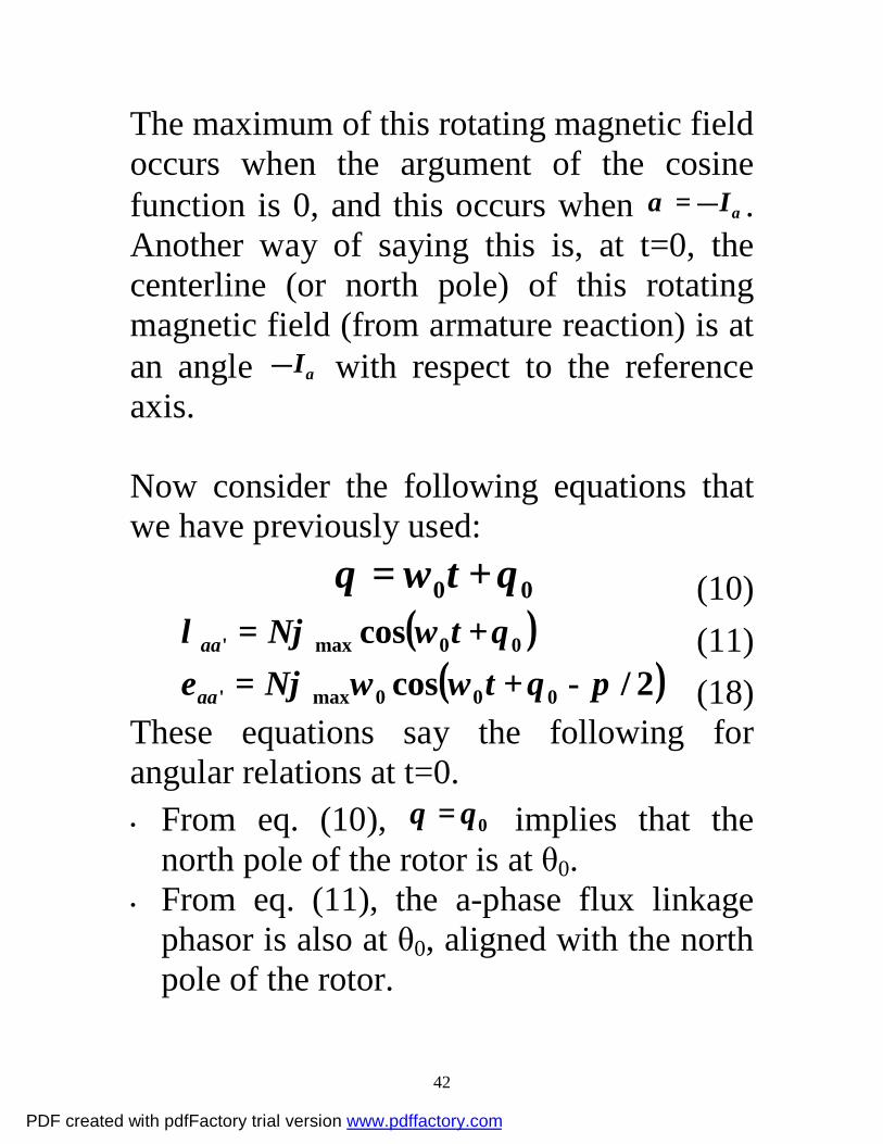
The maximum of this rotating magnetic field occurs when the argument of the cosine function is 0, and this occurs when aI∠=α . Another way of saying this is, at t=0, the centerline (or north pole) of this rotating magnetic field (from armature reaction) is at an angle aI∠ with respect to the reference axis. Now consider the following equations that we have previously used:

00 θωθ += t (10) ( )00max' cos θωϕλ += tNaa (11)

( )2/cos 000max' πθωωϕ −+= tNeaa (18) These equations say the following for angular relations at t=0. • From eq. (10), 0θθ = implies that the

north pole of the rotor is at θ0. • From eq. (11), the a-phase flux linkage

phasor is also at θ0, aligned with the north pole of the rotor.



43

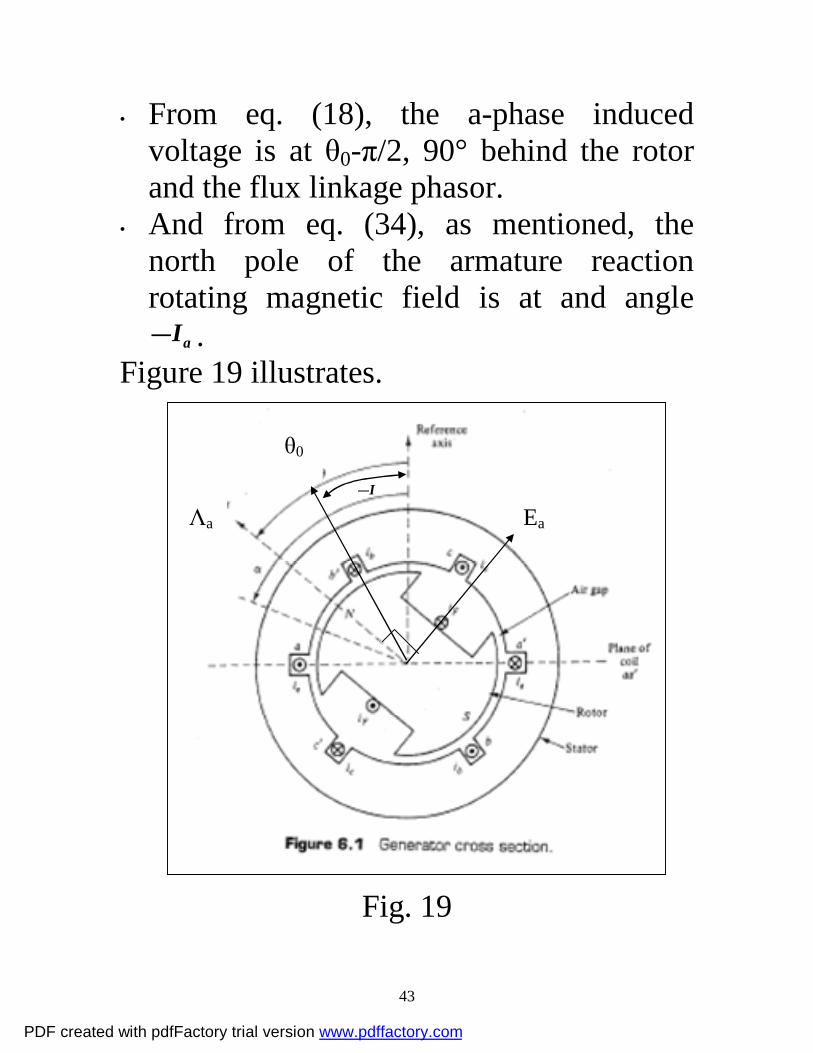
• From eq. (18), the a-phase induced voltage is at θ0-π/2, 90° behind the rotor and the flux linkage phasor.

• And from eq. (34), as mentioned, the north pole of the armature reaction rotating magnetic field is at and angle

aI∠ . Figure 19 illustrates.

θ0

I∠

Ea Λa

Fig. 19



44

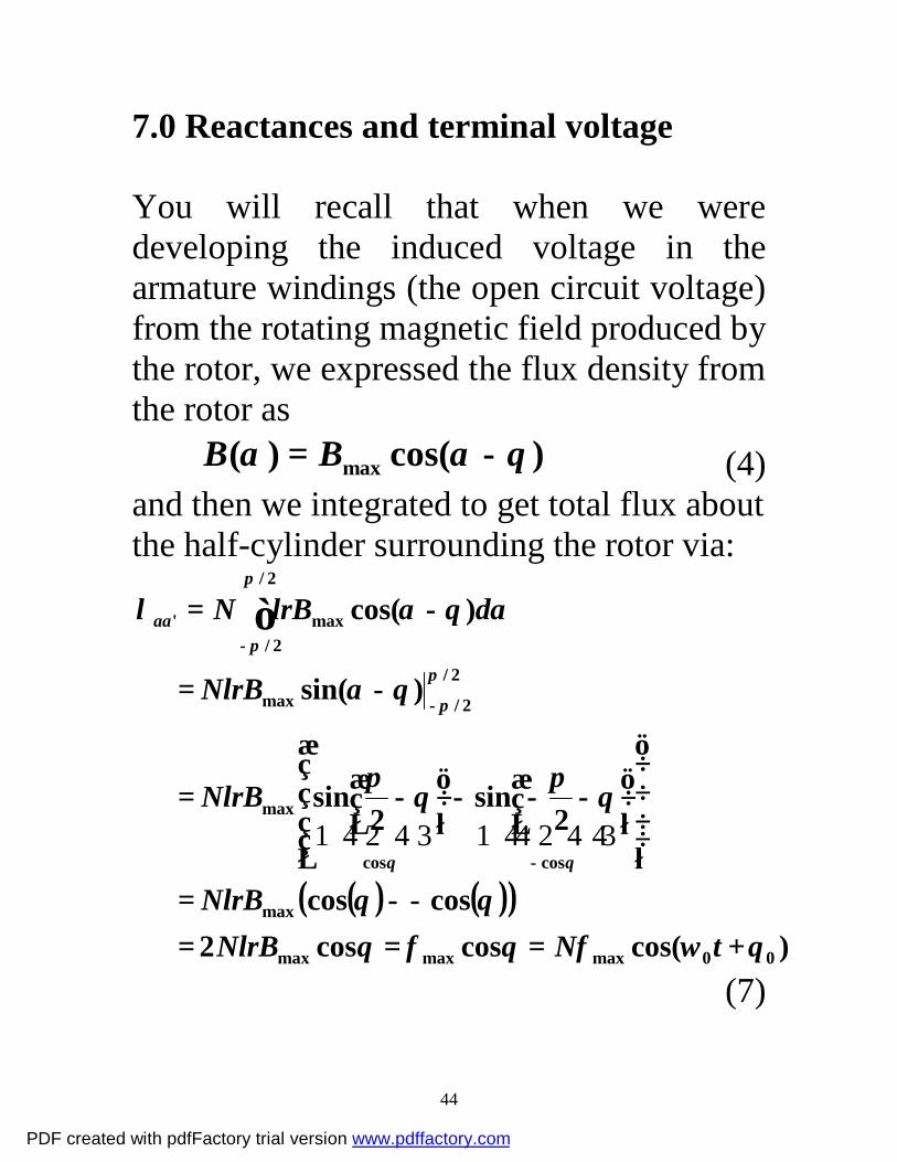
7.0 Reactances and terminal voltage You will recall that when we were developing the induced voltage in the armature windings (the open circuit voltage) from the rotating magnetic field produced by the rotor, we expressed the flux density from the rotor as

)cos()( max θαα −= BB (4) and then we integrated to get total flux about the half-cylinder surrounding the rotor via:

( ) ( )( ))cos(coscos2

coscos

2sin

2sin

)sin(

)cos(

00maxmaxmax

max

coscos

max

2/

2/max

2/

2/max'

θωφθφθ

θθ

θπ

θπ

θα

αθαλ

θθ

π

π

π

π

+===

−−=

−−−

−=

−=

−=

−

−

−∫

tNNlrBNlrB

NlrB

NlrB

dlrBNaa

443442143421

(7)



45

Finally, we used Faraday’s law to get

( )( )00max'

' cos θωϕλ

+−

=−= tNdt

ddt

de aaaa (12)

( )00max' sin θω += tEeaa (15)

The whole point of the above exercise was that the a-phase windings were experiencing flux linkages that varied with time, and this produced a voltage in which we were interested. Now the a-phase windings are seeing additional fields from armature reaction, and as we have shown, the composite of the fields from all three phases is a rotating magnetic field. Therefore the a-phase is experiencing flux linkages that vary with time (in addition to those from the rotor field) that are caused by the rotating magnetic field of armature reaction.



46

So let’s define λag as the total air-gap flux linkages seen by coil aa’. Then, as eq. (6.18) states in the text:

araaag λλλ += ' (35) where • λaa’ is the flux linkages from the rotating

magnetic field of the rotor • λar is the flux linkages from the rotating

magnetic field of armature reaction We want to obtain the voltage induced by the time variation in λag. This will be:

dtd

dtd

dtd

v araaagag

λλλ −+

−=

−= '

(36) But we have already obtained the first term in eq. (36); it was eaa’ as given by eq. (15). You will recall that we renamed this ea, and that we showed it had a phasor representation, from eq. (21), of

( )2/0 πθ −= jaa eEE (21)

So our job is only to obtain the second term in eq. (36).



47

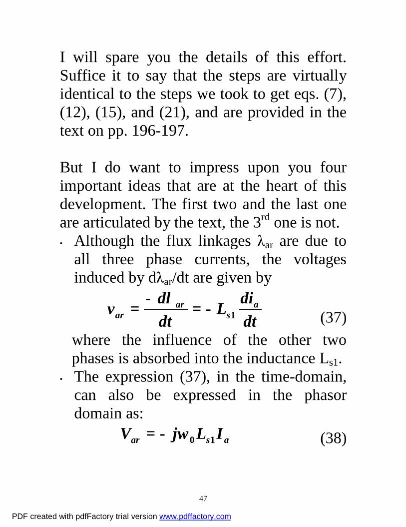
I will spare you the details of this effort. Suffice it to say that the steps are virtually identical to the steps we took to get eqs. (7), (12), (15), and (21), and are provided in the text on pp. 196-197. But I do want to impress upon you four important ideas that are at the heart of this development. The first two and the last one are articulated by the text, the 3rd one is not. • Although the flux linkages λar are due to

all three phase currents, the voltages induced by dλar/dt are given by

dtdiL

dtdv a

sar

ar 1−=−

=λ

(37) where the influence of the other two phases is absorbed into the inductance Ls1.

• The expression (37), in the time-domain, can also be expressed in the phasor domain as:

asar ILjV 10ω−= (38)



48

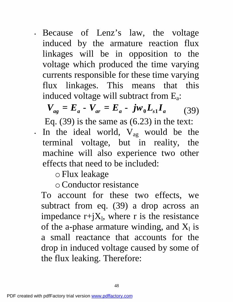
• Because of Lenz’s law, the voltage induced by the armature reaction flux linkages will be in opposition to the voltage which produced the time varying currents responsible for these time varying flux linkages. This means that this induced voltage will subtract from Ea:

asaaraag ILjEVEV 10ω−=−= (39) Eq. (39) is the same as (6.23) in the text:

• In the ideal world, Vag would be the terminal voltage, but in reality, the machine will also experience two other effects that need to be included:

o Flux leakage o Conductor resistance

To account for these two effects, we subtract from eq. (39) a drop across an impedance r+jXl, where r is the resistance of the a-phase armature winding, and Xl is a small reactance that accounts for the drop in induced voltage caused by some of the flux leaking. Therefore:



49

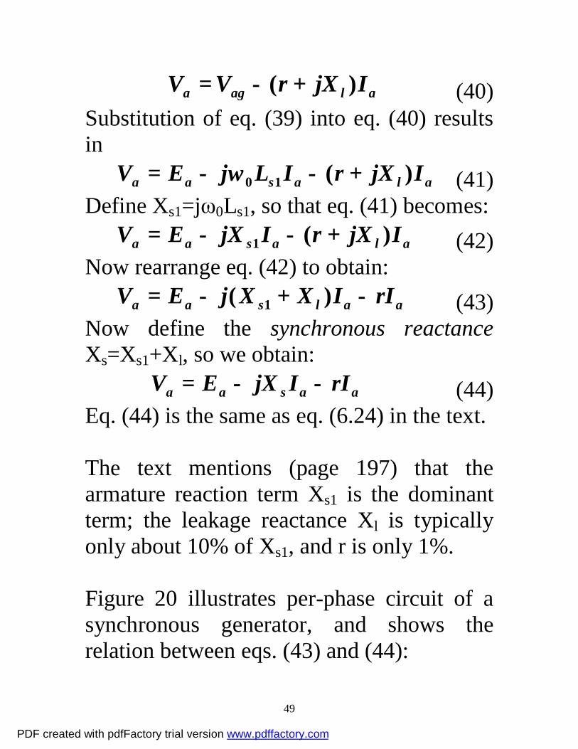
alaga IjXrVV )( +−= (40) Substitution of eq. (39) into eq. (40) results in

alasaa IjXrILjEV )(10 +−−= ω (41) Define Xs1=jω0Ls1, so that eq. (41) becomes:

alasaa IjXrIjXEV )(1 +−−= (42) Now rearrange eq. (42) to obtain:

aalsaa rIIXXjEV −+−= )( 1 (43) Now define the synchronous reactance Xs=Xs1+Xl, so we obtain:

aasaa rIIjXEV −−= (44) Eq. (44) is the same as eq. (6.24) in the text. The text mentions (page 197) that the armature reaction term Xs1 is the dominant term; the leakage reactance Xl is typically only about 10% of Xs1, and r is only 1%. Figure 20 illustrates per-phase circuit of a synchronous generator, and shows the relation between eqs. (43) and (44):



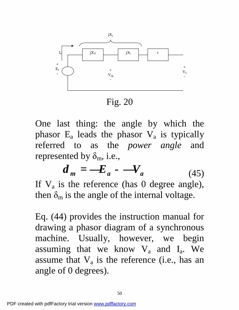
50

jXsl jXl r Ia

+ Va -

+ Ea -

+ Vag

-

jXs

Fig. 20

One last thing: the angle by which the phasor Ea leads the phasor Va is typically referred to as the power angle and represented by δm, i.e.,

aam VE ∠−∠=δ (45) If Va is the reference (has 0 degree angle), then δm is the angle of the internal voltage. Eq. (44) provides the instruction manual for drawing a phasor diagram of a synchronous machine. Usually, however, we begin assuming that we know Va and Ia. We assume that Va is the reference (i.e., has an angle of 0 degrees).



51

To obtain Ea from Va and Ia, we re-write eq. (44) like this:

aasaa rIIjXVE ++= (46) Now draw the Ea vector for the lagging condition (this means that Ia is lagging Va): Now draw the Ea vector for the leading condition (this means that Ia is leading Va):



52

What can you say about the relative magnitude of the field current in the two cases above? Lagging: Leading: What can you say about the strength of the magnetic field produced by the rotor winding, and the var supply, in the two cases above? Lagging: Leading: 8.0 Power for the smooth rotor case The per-phase equivalent circuit of Fig. 20 is simplified to that of Fig. 21:



53

jXs Ia

+ Va -

+ Ea -

Fig. 21

The complex power will be

**

−==

s

aaaaa jX

VEVIVS (47)

Assuming that Va is the reference, and with Ea=|Ea|(cosδm+jsinδm), we obtain:

*sincos

−+=

s

amamaa jX

VEjEVS

δδ(48)

Multiplying top and bottom by j we get:

*

*

sincos

sincos

+++−

=

−−−

=

s

amamaa

s

amamaa

XjVEEj

V

XjVEEj

VS

δδ

δδ



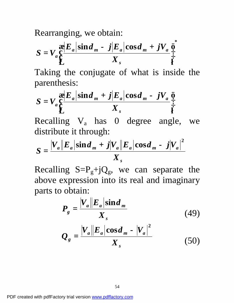
54

Rearranging, we obtain: *

cossin

+−=

s

amamaa X

jVEjEVS

δδ

Taking the conjugate of what is inside the parenthesis:

−+=

s

amamaa X

jVEjEVS

δδ cossin

Recalling Va has 0 degree angle, we distribute it through:

s

amaamaa

XVjEVjEV

S2cossin −+

=δδ

Recalling S=Pg+jQg, we can separate the above expression into its real and imaginary parts to obtain:

s

maag X

EVP

δsin= (49)

s

amaag X

VEVQ

2cos −=

δ (50)



55

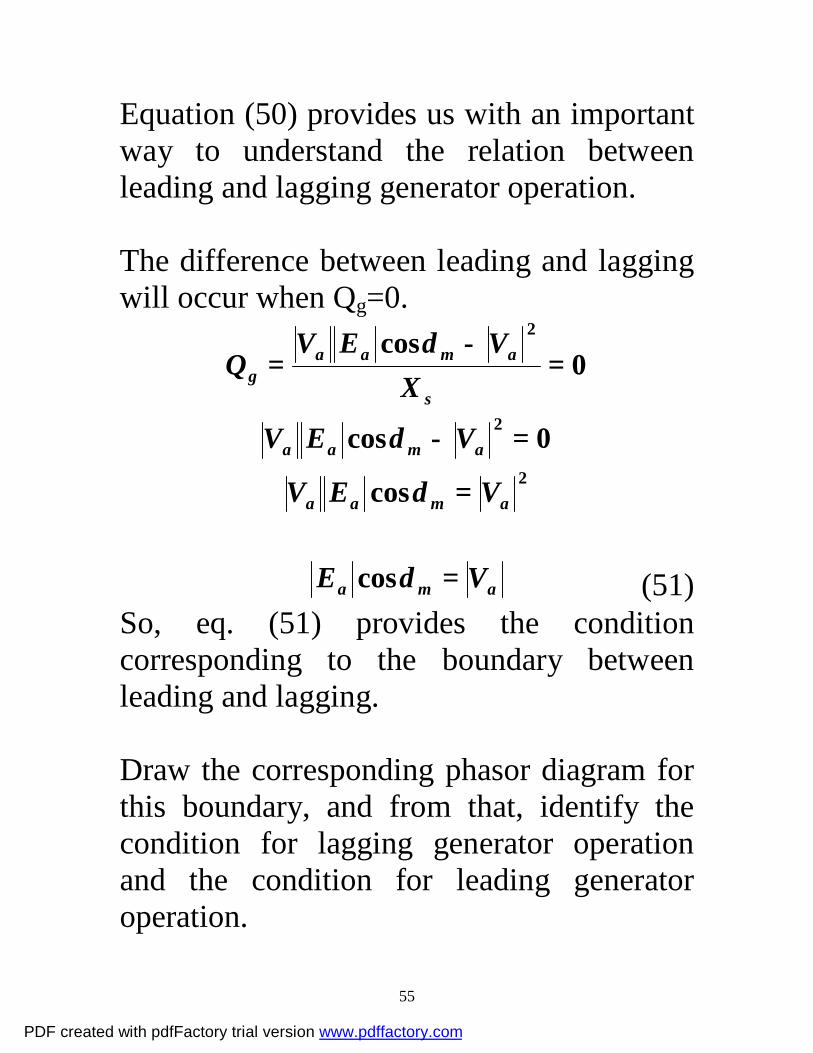
Equation (50) provides us with an important way to understand the relation between leading and lagging generator operation. The difference between leading and lagging will occur when Qg=0.

0cos 2

=−

=s

amaag X

VEVQ

δ

0cos 2=− amaa VEV δ 2cos amaa VEV =δ

ama VE =δcos (51)

So, eq. (51) provides the condition corresponding to the boundary between leading and lagging. Draw the corresponding phasor diagram for this boundary, and from that, identify the condition for lagging generator operation and the condition for leading generator operation.



56



57

9.0 Excitation control Moving between lagging and leading condition is performed via control of the generator field current, which produces the field flux fφ . Field current control can be done manually, but it is also done automatically via the excitation control system. The excitation control system is an automatic feedback control having the primary function of maintaining a predetermined terminal voltage by modifying the field current of the synchronous generator based on changes in the terminal voltage. Without excitation control, terminal voltage would fluctuate as a result of changes in Pg or external network conditions. The control is referred to as “negative feedback” because when terminal voltage increases, field current is decreased, and when terminal



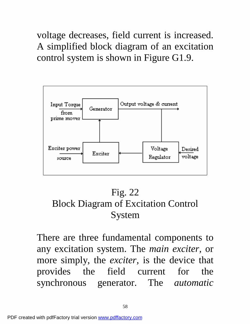
58

voltage decreases, field current is increased. A simplified block diagram of an excitation control system is shown in Figure G1.9.

Fig. 22 Block Diagram of Excitation Control

System

There are three fundamental components to any excitation system. The main exciter, or more simply, the exciter, is the device that provides the field current for the synchronous generator. The automatic



59

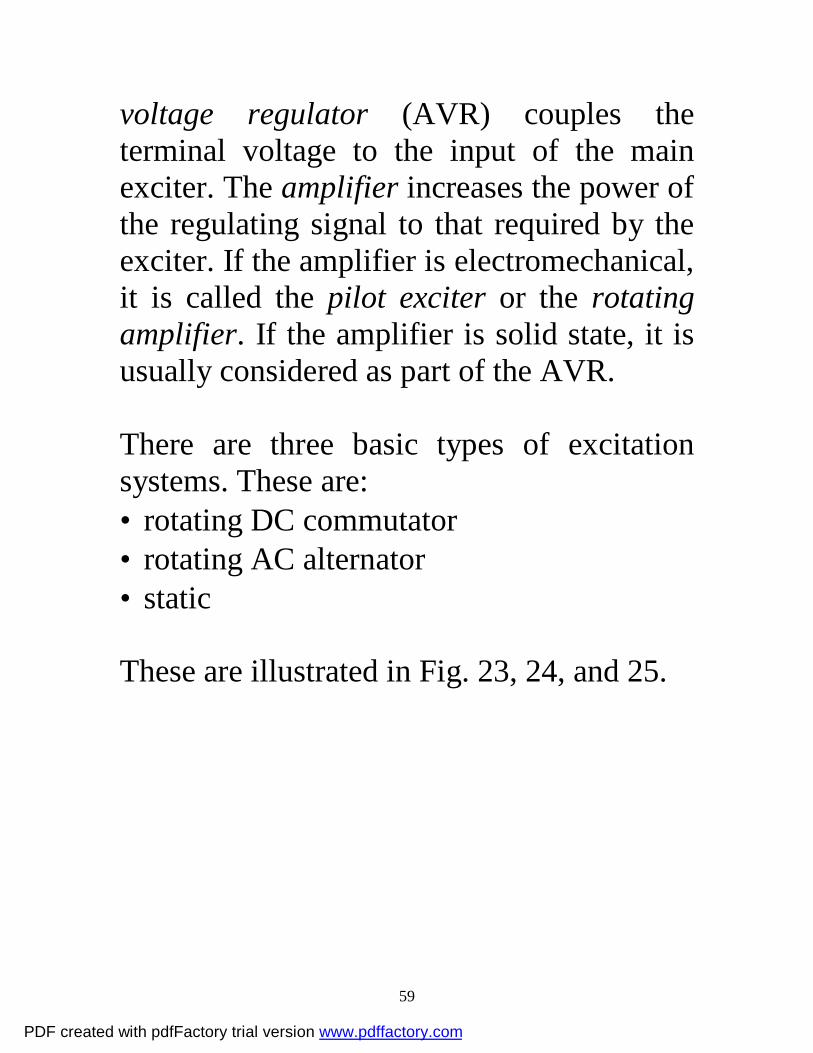
voltage regulator (AVR) couples the terminal voltage to the input of the main exciter. The amplifier increases the power of the regulating signal to that required by the exciter. If the amplifier is electromechanical, it is called the pilot exciter or the rotating amplifier. If the amplifier is solid state, it is usually considered as part of the AVR. There are three basic types of excitation systems. These are: • rotating DC commutator • rotating AC alternator • static These are illustrated in Fig. 23, 24, and 25.



60

Fig. 23 Rotating DC Commutator Type Excitation

System The DC commutator excitation system utilizes a DC generator mounted on the shaft of the synchronous generator to supply the field current. This type of system is no longer used in new facilities because it is slow in response, and because it requires high maintenance slip rings and brushes to couple the exciter output to the field windings.



61

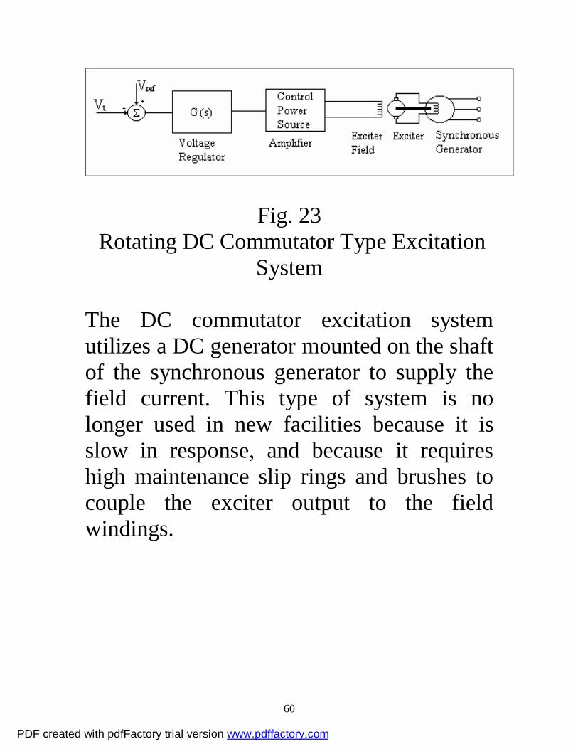
Fig. 24 Rotating AC Alternator Type Excitation

System The AC alternator excitation system uses an AC alternator with AC to DC rectification to supply the field winding of the synchronous generator. An important advantage over DC commutator systems is that AC alternator systems may be brushless, i.e., they do not use slip rings to couple the exciter to the rotor-mounted field winding. For example, the General Electric Althyrex uses an “inverted” alternator to supply the field voltage through a rectifier. The alternator is inverted in that, unlike the power generator, the field winding is on the stator and the



62

armature windings are on the rotor. Therefore the alternator field can be fed directly without the need for slip rings and brushes. Rectification to DC, required by the synchronous generator field, takes place by feeding the alternator three-phase output to a thyristor controlled bridge. The thyristor or silicon controlled rectifier (SCR) is similar to a diode, except that it remains “off” until a control signal is applied to the gate. The device will then conduct until current drops below a certain value or until the voltage across it reverses.

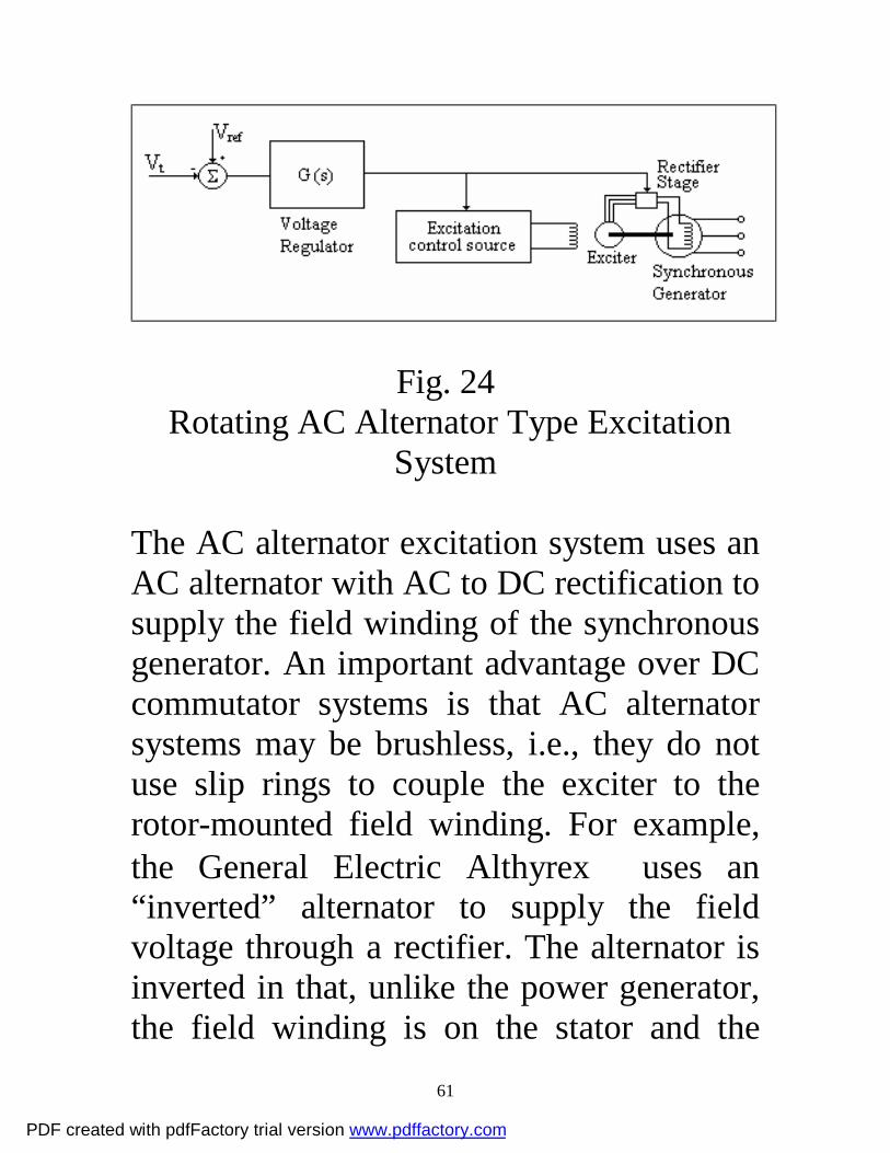
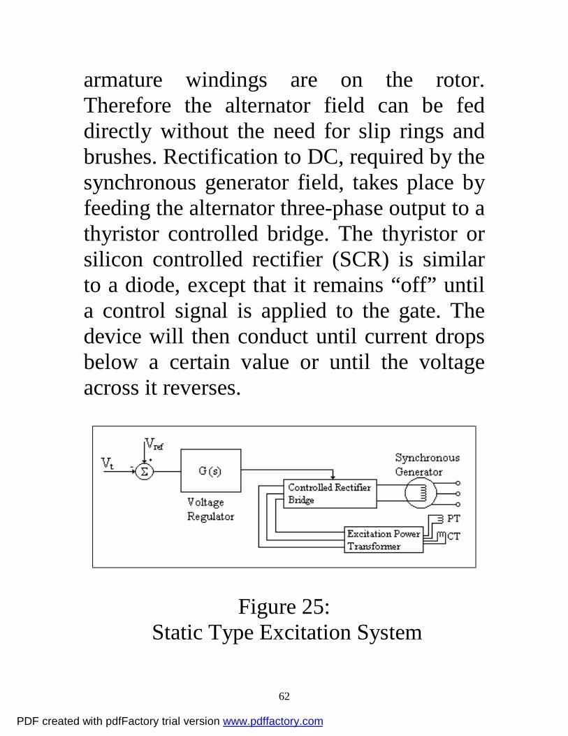
Figure 25: Static Type Excitation System



63

The third type of excitation system is called a static system because it is composed entirely of solid state circuitry, i.e., it contains no rotating device. The power source for this type of system is a potential and/or a current transformer supplied by the synchronous generator terminals. Three-phase power is fed to a rectifier, and the rectified DC output is applied to the synchronous generator field via slip rings and brushes. Static excitation systems are usually less expensive than AC alternator types, and the additional maintenance required by the slip rings and brushes is outweighed by the fact that static excitation systems have no rotating device. [1] http://geothermal.marin.org/GEOpresentation/ [2] A. Fitzgerald, C. Kingsley, and A. Kusko, “Electric Machinery, Processes, Devices, and Systems of Electromechanical Energy Conversion,” 3rd edition, 1971, McGraw Hill. [3] S. Chapman, “Electric Machinery Fundamentals,” 1985, McGraw-Hill.


http://geothermal.marin.org/GEOpresentation/


Synchronous Machines 1.0 Introductionhome.eng.iastate.edu/~jdm/EE456/SynchMachines.pdf1 Synchronous Machines 1.0 Introduction One might easily argue that the synchronous generator

Documents