Synchronization of weakly coupled oscillators: coupling ... [email protected] and [email protected] Received 13 July 2013, in final form 2 October 2013 Published 26 November 2013Published

This content has been downloaded from IOPscience. Please scroll down to see the full text.

Download details:

IP Address: 128.84.94.80

This content was downloaded on 06/12/2013 at 20:19

Please note that terms and conditions apply.

Synchronization of weakly coupled oscillators: coupling, delay and topology

View the table of contents for this issue, or go to the journal homepage for more

2013 J. Phys. A: Math. Theor. 46 505101

(http://iopscience.iop.org/1751-8121/46/50/505101)

Home Search Collections Journals About Contact us My IOPscience

IOP PUBLISHING JOURNAL OF PHYSICS A: MATHEMATICAL AND THEORETICAL

J. Phys. A: Math. Theor. 46 (2013) 505101 (24pp) doi:10.1088/1751-8113/46/50/505101

Synchronization of weakly coupled oscillators:coupling, delay and topology

Enrique Mallada and Ao Tang

School of ECE, Cornell University, Ithaca, NY 14853, USA

E-mail: [email protected] and [email protected]

Received 13 July 2013, in final form 2 October 2013Published 26 November 2013Online at stacks.iop.org/JPhysA/46/505101

AbstractThere are three key factors in a system of coupled oscillators that characterizethe interaction between them: coupling (how to affect), delay (when to affect)and topology (whom to affect). The existing work on each of these factors hasmainly focused on special cases. With new angles and tools, this paper makesprogress in relaxing some assumptions on these factors. There are three mainresults in this paper. Firstly, by using results from algebraic graph theory, asufficient condition is obtained that can be used to check equilibrium stability.This condition works for arbitrary topology, generalizing existing results andalso leading to a sufficient condition on the coupling function which guaranteesthat the system will reach synchronization. Secondly, it is known that identicaloscillators with sin() coupling functions are guaranteed to synchronize in phaseon a complete graph. Our results prove that in many cases certain structures suchas symmetry and concavity, rather than the exact shape of the coupling function,are the keys for global synchronization. Finally, the effect of heterogenousdelays is investigated. Using mean field theory, a system of delayed coupledoscillators is approximated by a non-delayed one whose coupling depends onthe delay distribution. This shows how the stability properties of the systemdepend on the delay distribution and allows us to predict its behavior. Inparticular, we show that for sin() coupling, heterogeneous delays are equivalentto homogeneous delays. Furthermore, we can use our novel sufficient instabilitycondition to show that heterogeneity, i.e. wider delay distribution, can helpreach in-phase synchronization.

PACS number: 05.45.Xt

(Some figures may appear in colour only in the online journal)

1751-8113/13/505101+24$33.00 © 2013 IOP Publishing Ltd Printed in the UK & the USA 1

J. Phys. A: Math. Theor. 46 (2013) 505101 E Mallada and A Tang

1. Introduction

Systems of coupled oscillators have been widely studied in different disciplines ranging frombiology [1–5] and chemistry [6, 7] to engineering [8, 9] and physics [10, 11]. The possiblebehavior of such systems can be complex. For example, the intrinsic symmetry of the networkcan produce multiple limit cycles or equilibria with relatively fixed phases (phase-lockedtrajectories) [12], which in many cases can be stable [13]. Also, the heterogeneity in thenatural oscillation frequency can lead to incoherence [14] or even chaos [15].

A particularly interesting question is whether the coupled oscillators will synchronize inphase in the long run [16–20]. Besides its clear theoretical value, it also has rich applicationsin practice.

In essence, there are three key factors in a system of coupled oscillators that characterizethe interaction between oscillators: coupling, delay and topology. For each of these, the existingwork has mainly focused on special cases as explained below. In this paper, further researchwill be discussed on each of the three factors.

• Topology (whom to affect, section 3.2). Current results either restrict to complete graph or aring topology for analytical tractability [19], study local stability of topology independentsolutions over time-varying graph [21–23], or introduce dynamic controllers to achievesynchronization for time-varying uniformly connected graphs [24, 25]. We develop agraph-based sufficient condition which can be used to check equilibrium instability forany fixed topology. It also leads to a family of coupling functions guaranteeing that thesystem will reach global phase consensus for arbitrary connected undirected graphs usingonly physically meaningful state variables.

• Coupling (how to affect, section 3.3). The classical Kuramoto model [14] assumes a sin()

coupling function. Our study suggests that certain symmetry and convexity structuressuffice to guarantee global synchronization. We show that most orbits that appear due tosymmetries on a complete graph are unstable provided that the coupling function is evenand concave on [0, π ] and its derivative is concave on [−π

2 , π2 ].

• Delay (when to affect, section 4). Existing work generally assumes zero delay amongoscillators or requires them to be bounded up to a constant fraction of the period [26].This is clearly unsatisfactory especially if the oscillating frequencies are high. We usemean field theory to study unbounded delays by constructing a non-delayed phase modelthat is equivalent to the original one in the large population limit. Using this noveltechnique, we then show that when the system has sin() coupling, heterogeneous delaysand homogeneous delays are equivalent. Finally, we use our novel graph-based instabilitycondition to illustrate how a slight increase in the heterogeneity of the delays can makecertain non-in-phase equilibria unstable and therefore promote in-phase synchronization.

This paper focuses on weakly coupled oscillators, which can be either pulse-coupled orphase-coupled. Although most of the results presented are for phase-coupled oscillators, theycan be readily extended for pulse-coupled oscillators (see, e.g., [27, 28]). It should be notedthat results in section 3 are independent of the strength of the coupling and therefore do notrequire inclusion of the weak coupling assumption. Preliminary versions of this work havebeen presented in [29, 30].

The paper is organized as follows. We describe pulse-coupled and phase-coupled oscillatormodels, as well as their common weak coupling approximation, in section 2. Using some factsfrom algebraic graph theory and potential dynamics in section 3.1, we present the negative cutinstability theorem in section 3.2.1 to check whether an equilibrium is unstable. This leads totheorem 1 in section 3.2.2 which identifies a class of coupling functions that guarantee that

2

J. Phys. A: Math. Theor. 46 (2013) 505101 E Mallada and A Tang

the system always synchronizes in phase. It is well known that the Kuramoto model producesglobal synchronization over a complete graph. In section 3.3, we demonstrate that a largeclass of coupling functions, in which the Kuramoto model is a special case, guarantee theinstability of most of the limit cycles in a complete graph network. Section 4 is devoted tothe discussion of the effect of delay. An equivalent non-delayed phase model is constructedwhose coupling function is the convolution of the original coupling function and the delaydistribution. Using this approach, we show that for the Kuramoto model (with homogeneousfrequencies), heterogeneous delays and homogeneous delays are equivalent (section 4.1).Finally, we show in section 4.2 that sometimes more heterogeneous delays among oscillatorscan help reach synchronization. Our conclusions are presented in section 5.

2. Coupled oscillators

We consider two different models of coupled oscillators analyzed in the literature. Thedifference between the models arises in the interactions between the oscillators, and theirdynamics can be quite different. However, when the interactions are weak (weak coupling),both systems behave similarly and share the same approximation. This allows us to study themunder a common framework.

Each oscillator is represented by a phase θi in the unit circle S1 which in the absence ofcoupling moves with constant speed θi = ω. Here, S1 represents the unit circle, or equivalentlythe interval [0, 2π ] with 0 and 2π identified (0 ≡ 2π ), and ω = 2π

T denotes the naturalfrequency of the oscillation.

2.1. Pulse-coupled oscillators

In this model the interaction between oscillators is performed by pulses. An oscillator j sendsout a pulse whenever it crosses zero (θ j = 0). When oscillator i receives a pulse, it will changeits position from θi to θi + εκi j(θi). The function κi j represents how other oscillator actionsaffect oscillator i and the scalar ε > 0 is a measure of the coupling strength. These jumpscan be modeled by a Dirac delta function δ satisfying δ(t) = 0 ∀t �= 0, δ(0) = +∞, and∫

δ(s)ds = 1. The coupled dynamics are represented by

θi(t) = ω + εω∑j∈Ni

κi j(θi(t))δ(θ j(t − ηi j)), (1)

where ηi j > 0 is the propagation delay between oscillators i and j (ηi j = η ji), and Ni isthe set of i’s neighbors. The factor of ω in the sum is needed to keep the size of the jumpwithin εκi j(θi). This is because θ j(t) behaves like ωt when crosses zero and therefore the jumpproduced by δ(θ j(t)) is of size

∫δ(θ j(t))dt = ω−1 [28].

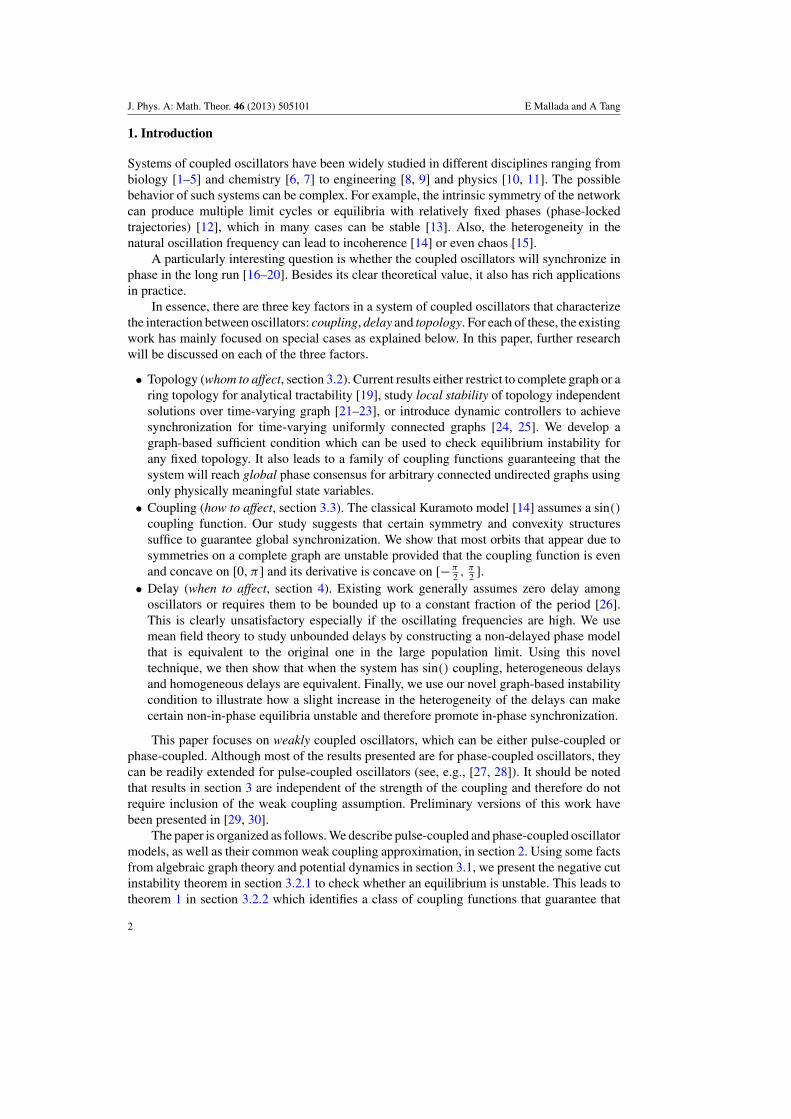
The coupling function κi j can be classified based on the qualitative effect it produces inthe absence of delay. After one period, if the net effect of the mutual jumps brings a pair ofoscillators closer, we call it attractive coupling. If the oscillators are brought further apart, itis considered to be repulsive coupling. The former can be achieved, for instance, if κi j(θ ) � 0for θ ∈ [0, π ) and κi j(θ ) � 0 for θ ∈ [π, 2π). See figure 1 for an illustration of an attractivecoupling κi j and its effect on the relative phases.

This pulse-like interaction between oscillators was first introduced by Peskin [2] in 1975as a model of the pacemaker cells of the heart, although the canonic form did not appear inthe literature until 1999 [28]. In general, when the number of oscillators is large, there areseveral different limit cycles besides the in-phase synchronization and many of them can bestable [13].

3

J. Phys. A: Math. Theor. 46 (2013) 505101 E Mallada and A Tang

Figure 1. Pulse-coupled oscillators with attractive coupling. The jumps of oscillators i and j areillustrated at the top. The bottom charts show the value of the coupling function at the instantswhen either j or i send a pulse. After one cycle, both oscillators end up closer (attractive coupling).

The question of whether this system can collectively achieve in-phase synchronizationwas answered for the complete graph case and zero delay by Mirollo and Strogatz in 1990[20]. They showed that if κi j(θ ) is strictly increasing on (0, 2π) with a discontinuity in 0(which resembles attractive coupling), then for almost every initial condition, the system cansynchronize in phase in the long run.

The two main assumptions of [20] are all to all communication and zero delay. Whetherin-phase synchronization can be achieved for arbitrary graphs has been an open problem forover twenty years. On the other hand, when delay among oscillators is introduced the analysisbecomes intractable. Even in the case of two oscillators, there is a large number of possibilitiesto be considered [31, 32].

2.2. Phase-coupled oscillators

In the model of phase-coupled oscillators, the interaction between neighboring oscillators iand j ∈ Ni is modeled by change of the oscillating speeds. Although the speed change cangenerally be a function of both phases (θi, θ j), we concentrate on the case where the speedchange is a function of the phase differences fi j(φ j(t −ηi j)−φi(t)). Thus, since the net speedchange of oscillator i amounts to the sum of the effects of its neighbors, the full dynamics isdescribed by

φi(t) = ω + ε∑j∈Ni

fi j(φ j(t − ηi j) − φi(t)). (2)

The function fi j is usually called coupling function, and as before ηi j represents delay and Ni

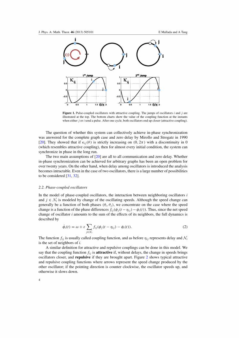
is the set of neighbors of i.A similar definition for attractive and repulsive couplings can be done in this model. We

say that the coupling function fi j is attractive if, without delays, the change in speeds bringsoscillators closer, and repulsive if they are brought apart. Figure 2 shows typical attractiveand repulsive coupling functions where arrows represent the speed change produced by theother oscillator; if the pointing direction is counter clockwise, the oscillator speeds up, andotherwise it slows down.

4

J. Phys. A: Math. Theor. 46 (2013) 505101 E Mallada and A Tang

Figure 2. Phase-coupled oscillators with attractive and repulsive coupling. The mutual influenceof oscillators i and j is illustrated at the top for both attractive (left) and repulsive (right) coupling.The bottom charts show the corresponding coupling functions.

When fi j = KN sin(), K > 0 (attractive coupling), this model is known as the classical

Kuramoto model [33]. Intensive research has been conducted on this model, but convergenceresults are usually limited to cases with all to all coupling (Ni = N \{i}, i.e., complete graphtopology) and no delay (ηi j = 0), see e.g. [19, 34], or to some regions of the state space [26].

2.3. Weak coupling approximation

We now concentrate in the regime in which the coupling strength of both models is weak, i.e.1 � ε > 0. For pulse-coupled oscillators, this implies that the effect of the jumps originatedby each neighbor can be approximated by their average [27]. For phase-coupled oscillators, itimplies that to the first order φi(t − ηi j) is well approximated by φi(t) − ωηi j.

The effect of these approximations allows us to completely capture the behavior of bothsystems using the following equation where we assume that every oscillator has the samenatural frequency ω and only keep track of the relative difference using

φi = ε∑j∈Ni

fi j(φ j − φi − ψi j). (3)

For pulse-coupled oscillators, the coupling function is given by

fi j(θ ) = ω

2πκi j(−θ ), (4)

and the phase lag ψi j = ωηi j represents the distance that oscillator i’s phase can travel alongthe unit circle during the delay time ηi j. Equation (4) also shows that the attractive/repulsivecoupling classifications of both models are in fact equivalent, since in order to produce thesame effect κi j and fi j should be mirrored, as illustrated in figures 1 and 2.

Equation (3) captures the relative change of the phases and therefore any solution to (3)can be immediately translated to either (1) or (2) by adding ωt. For example, if φ∗ is anequilibrium of (3), by adding ωt, we obtain a limit cycle in the previous models. Besidesthe delay interpretation for ψi j, (3) is also known as a system of coupled oscillators withfrustration, see e.g. [35].

From now on we will concentrate on (3) with the understanding that any convergenceresult derived will be immediately true for the original models in the weak coupling limit. We

5

J. Phys. A: Math. Theor. 46 (2013) 505101 E Mallada and A Tang

are interested in the attracting properties of phase-locked invariant orbits within T N , whichcan be represented by φ(t) = ω∗t1N + φ∗, where 1N = (1, . . . , 1)T ∈ T N , and φ∗ and ω∗ aresolutions to

ω∗ = ε∑j∈Ni

fi j(φ∗j − φ∗

i − ψi j), ∀i. (5)

Whenever the system reaches one of these orbits, we say that it is synchronized or phase-locked. Additionally, if all the elements of φ∗ are equal, we say that the system is synchronizedin-phase or that it is in-phase locked. It is easy to check that for a given equilibrium φ∗ of(3), any solution of the form φ∗ + λ1N , with λ ∈ R, is also an equilibrium that identifies thesame limit cycle. Therefore, two equilibria φ1,∗ and φ2,∗ will be considered to be equivalent,if both identifies the same orbit, or equivalently, if both belongs to the same connected set ofequilibria

Eφ∗ := {φ ∈ T N |φ = φ∗ + λ1N, λ ∈ R}. (6)

3. Effect of topology and coupling

In this section we concentrate on the class of coupling functions fi j that are symmetric ( fi j = f ji

∀i j), odd ( fi j(−θ ) = − fi j(θ )) and continuously differentiable. We also assume that there isno delay within the network, i.e. ψi j = 0 ∀i j. Thus, (3) is reduced to

φi = ε∑j∈Ni

fi j(φ j − φi). (7)

Remark 1. While the continuous differentiable assumption on fi j is technical, the symmetryand odd assumptions have an intuitive interpretation: When fi j is symmetric and odd, theeffect of the oscillator j in i ( fi j(φ j − φi)) is equal in magnitude and opposite in sign to theeffect of i in j ( f ji(φi − φ j)), i.e. fi j(φ j − φi) = f ji(φ j − φi) = − f ji(φi − φ j). In other words,there is a reciprocity in their mutual effect.

In the rest of this section we progressively show how with some extra conditions on fi j wecan guarantee in-phase synchronization for arbitrary undirected graphs. Since we know thatthe network can have many other phase-locked trajectories besides the in-phase one, our targetis an almost global stability result [36], meaning that the set of initial conditions that doesnot eventually lock in phase has zero measure. Later we show how most of the phase-lockedsolutions that appear on a complete graph are unstable under some general conditions on thestructure of the coupling function.

3.1. Preliminaries

We now introduce some prerequisites used in our later analysis.

3.1.1. Algebraic graph theory. We start by reviewing basic definitions and properties fromgraph theory [37, 38] that are used in the paper. Let G be the connectivity graph that describesthe coupling configuration. We use V (G) and E(G) to denote the set of vertices (i or j)and undirected edges (e) of G. An undirected graph G can be directed by giving a specificorientation σ to the elements in the set E(G). That is, for any given edge e ∈ E(G), wedesignate one of the vertices to be the head and the other one to be the tail giving Gσ .

Although in the following definitions we need to give graph G a given orientation σ ,the underlying connectivity graph of the system is assumed to be undirected. This is not a

6

J. Phys. A: Math. Theor. 46 (2013) 505101 E Mallada and A Tang

problem as the properties used in this paper are independent of a particular orientation σ andthey are therefore properties of the undirected graph G. Thus, to simplify notation we drop thesuperscript σ from Gσ with the understanding that G is now an induced directed graph withsome fixed—but arbitrarily chosen—orientation.

We use P = (V −,V +) to denote a partition of the vertex set V (G) such thatV (G) = V − ∪ V + and V − ∩ V + = ∅. The cut C(P) associated with P, or equivalentlyC(V −,V +), is defined as C(P) := {i j ∈ E(G)|i ∈ V −, j ∈ V +, or vice versa.}. Each partitioncan be associated with a vector column cP where cP(e) = 1 if e goes from V − to V +,cP(e) = −1 if e goes from V + to V − and cP(e) = 0 if e stays within either set.

There are several matrices associated with the oriented graph G that embed informationabout its topology. However, the most significant one for our present work is the orientedincidence matrix B ∈ R|V (G)|×|E(G)| where B(i, e) = 1 if i is the head of e, B(i, e) = −1 if i isthe tail of e and B(i, e) = 0 otherwise.

3.1.2. Potential dynamics. We now describe how our assumptions on fi j not only simplifythe dynamics considerably, but also allow us to use the graph theory properties introduced insection 3.1.1 to gain a deeper understanding of (3).

While fi j being continuously differentiable is standard in order to study local stabilityand sufficient to apply LaSalle’s invariance principle [39], the symmetry and odd assumptionshave a stronger effect on the dynamics.

For example, under these assumptions the system (7) can be compactly rewritten in avector form as

φ = −εBF(BT φ), (8)

where B is the adjacency matrix defined in section 3.1.1 and the map F : E (G) → E (G) is

F(y) = ( fi j(yi j))i j∈E(G).

This new representation has several properties. First, from the properties of B onecan easily show that (5) can only hold with ω∗ = 0 for arbitrary graphs [16] (sinceNω∗ = ω∗1T

N1N = −ε1TNBF(BT φ) = 0), which implies that every phase-locked solution

is an equilibrium of (7) and that every limit cycle of the original system (3) can be representedby some E∗

φ on (7).However, the most interesting consequence of (8) comes from interpreting F(y) as the

gradient of a potential function

W (y) =∑

i j∈E(G)

∫ yi j

0fi j(s) ds.

Then, by defining V (φ) = (W ◦ BT )(φ) = W (BT φ), (8) becomes a gradient descent law forV (φ), i.e.,

φ = −εBF(BT φ) = −εB∇W (BT φ) = −ε∇V (φ),

where in the last step above we used the property ∇(W ◦ BT )(φ) = B∇W (BT φ). This makesV (φ) a natural Lyapunov function candidate since

V (φ) = 〈∇V (φ), φ〉 = −ε|∇V (φ)|2 = −1

ε|φ|2 � 0. (9)

Furthermore, since the trajectories of (8) are constrained into the N-dimensional torusT N , which is compact, V (φ) satisfies the hypothesis of LaSalle’s invariance principle(theorem 4.4 [39]), i.e. there is a compact positively invariant set, T N and a functionV : T N → R that decreases along the trajectories φ(t). Therefore, for every initial condition,the trajectory converges to the largest invariant set M within {V ≡ 0} which is the equilibriaset E = {φ ∈ T N |φ ≡ 0} = ⋃

φ∗ Eφ∗ .

7

J. Phys. A: Math. Theor. 46 (2013) 505101 E Mallada and A Tang

Remark 2. The fact that symmetric and odd coupling induces potential dynamics is wellknown in the physics community [40]. However, it has also been rediscovered in the controlcommunity [17] for the specific case of sine coupling. Clearly, this does not suffice to showalmost global stability, since it is possible to have other stable phase-locked equilibrium setsbesides the in-phase one. However, if we can show that all the non-in-phase equilibria areunstable, then almost global stability follows. That is the focus of the next section.

3.2. Negative cut instability condition

We now present the main results of this section. Our technique can be viewed as a generalizationof [19]. By means of algebraic graph theory, we provide a better stability analysis of theequilibria under a more general framework. We further use the new stability results tocharacterize fi j that guarantees almost global stability.

3.2.1. Local stability analysis. In this section we develop the graph theory based tools tocharacterize the stability of each equilibrium. We will show that given an equilibrium φ∗ ofthe system (8), with connectivity graph G and fi j as described in this section, if there exists acut C(P) such that the sum∑

i j∈C(P)

f ′i j(φ

∗j − φ∗

i ) < 0, (10)

the equilibrium φ∗ is unstable.Consider first an equilibrium point φ∗. Then, the first order approximation of (8) around

φ∗ is

δφ = −εB

[∂

∂yF(BT φ∗)

]BT δφ,

where δφ := φ − φ∗ is the incremental phase variable, and ∂∂y F(BT φ∗) ∈ R|E(G)|×|E(G)|is the

Jacobian of F(y) evaluated at BT φ∗, i.e., ∂∂y F(BT φ∗) = diag({ f ′

i j(φ∗j − φ∗

i )}i j∈E(G)).

Now let A = −εB[ ∂∂y F(BT φ∗)]BT and consider the linear system δφ = Aδφ.Although it

is possible to numerically calculate the eigenvalues of A given φ∗ to study the stability, herewe use the special structure of A to provide a sufficient condition for instability that has nicegraph-theoretical interpretations.

Since A is symmetric, it is straight-forward to check that A has at least one positiveeigenvalue, i.e. φ∗ is unstable, if and only if xT Ax > 0. Now, given any partition P = (V −,V +),consider the associated vector cP, define xP such that xi = 1

2 if i ∈ V + and xi = − 12 if i ∈ V −.

Then it follows from the definition of B that cP = BT xP which implies that−1

εxT

PAxP = cTP

[∂

∂yF(BT φ∗)

]cP =

∑i j∈C(P)

f ′i j(φ

∗j − φ∗

i ).

Therefore, when condition (10) holds, A = −εBDBT has at least one eigenvalue whosereal part is positive.

Remark 3. Equation (10) provides a sufficient condition for instability; it is not clear whathappens when (10) does not hold. However, it gives a graph-theoretical interpretation that canbe used to provide stability results for general topologies. That is, if the minimum cut cost isnegative, the equilibrium is unstable.

Remark 4. Since the weights of the graph f ′i j(φ

∗j − φ∗

i ) are functions of the phase difference,(10) holds for any equilibria of the form φ∗ +λ1N . Thus, the result holds for the whole set Eφ∗

defined in (6).

8

J. Phys. A: Math. Theor. 46 (2013) 505101 E Mallada and A Tang

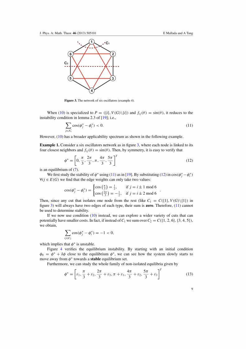
Figure 3. The network of six oscillators (example 4).

When (10) is specialized to P = ({i},V (G)\{i}) and fi j(θ ) = sin(θ ), it reduces to theinstability condition in lemma 2.3 of [19]; i.e.,∑

j∈Ni

cos(φ∗j − φ∗

i ) < 0. (11)

However, (10) has a broader applicability spectrum as shown in the following example.

Example 1. Consider a six oscillators network as in figure 3, where each node is linked to itsfour closest neighbors and fi j(θ ) = sin(θ ). Then, by symmetry, it is easy to verify that

φ∗ =[

0,π

3,

2π

3, π,

4π

3,

5π

3

]T

(12)

is an equilibrium of (7).We first study the stability of φ∗ using (11) as in [19]. By substituting (12) in cos(φ∗

j −φ∗i )

∀i j ∈ E(G) we find that the edge weights can only take two values:

cos(φ∗j − φ∗

i ) ={

cos(

π3

) = 12 , if j = i ± 1 mod 6

cos(

2π3

) = − 12 , if j = i ± 2 mod 6

.

Then, since any cut that isolates one node from the rest (like C1 = C({1},V (G)\{1}) infigure 3) will always have two edges of each type, their sum is zero. Therefore, (11) cannotbe used to determine stability.

If we now use condition (10) instead, we can explore a wider variety of cuts that canpotentially have smaller costs. In fact, if instead of C1 we sum over C2 = C({1, 2, 6}, {3, 4, 5}),we obtain, ∑

i j∈C2

cos(φ∗j − φ∗

i ) = −1 < 0,

which implies that φ∗ is unstable.Figure 4 verifies the equilibrium instability. By starting with an initial condition

φ0 = φ∗ + δφ close to the equilibrium φ∗, we can see how the system slowly starts tomove away from φ∗ towards a stable equilibrium set.

Furthermore, we can study the whole family of non-isolated equilibria given by

φ∗ =[ε1,

π

3+ ε2,

2π

3+ ε3, π + ε1,

4π

3+ ε2,

5π

3+ ε3

]T

(13)

9

J. Phys. A: Math. Theor. 46 (2013) 505101 E Mallada and A Tang

0 1 2 3 4 5 6 7 8 9 10−0.5

0

0.5

1

1.5

2 1 2 3 4 5 6

t

φi

π

Figure 4. Unstable equilibrium φ∗. Initial condition φ0 = φ∗+δp, where δp is a small perturbation.The small perturbation gets amplified showing that the equilibrium is unstable.

Figure 5. Minimum cut value C∗(λ1, λ2) showing that the equilibria (13) are unstable.

where ε1, ε2, ε3 ∈ R, which due to remark 4, we can reduce (13) to

φ∗ =[

0,π

3+ λ1,

2π

3+ λ2, π,

4π

3+ λ1,

5π

3+ λ2

]T

(14)

with λ1 = ε2 − ε1 and λ2 = ε3 − ε1.Instead of focusing on only one cut, here we compute the minimum cut value (10) over

the 31 possible cuts, i.e. C∗(λ1, λ2) := minP∑

i j∈C(P) f ′i j(φ j(λ1, λ2)

∗ − φ∗i (λ1, λ2)). Figure 5

shows the value of C∗(λ1, λ2) for λi ∈ [−π, π ]. Since C∗(λ1, λ2) is 2π -periodic on eachvariable and its value is negative for every λ1, λ2 ∈ [−π, π ], the family of equilibria (14) (andconsequently (13)) is unstable.

3.2.2. Almost global stability. Condition (10) also provides insight on which class of couplingfunctions can potentially give us almost global convergence to the in-phase equilibrium setE1N . If it is possible to find some fi j with f ′

i j(0) > 0, such that for any non-in-phase equilibriumφ∗, there is a cut C with

∑i j∈C f ′

i j(φ∗j − φ∗

i ) < 0, then the in-phase equilibrium set will bealmost globally stable [13]. The main difficulty is that for general fi j and arbitrary network G,it is not easy to locate every phase-locked equilibria and it is therefore not simple to know inwhat region of the domain of fi j the slope should be negative.

10

J. Phys. A: Math. Theor. 46 (2013) 505101 E Mallada and A Tang

We now concentrate on the one-parameter family of functions Fb, with b ∈ (0, π ), suchthat fi j ∈ Fb whenever fi j is symmetric, odd, continuously differentiable and

• f ′i j(θ; b) > 0,∀θ ∈ (0, b) ∪ (2π − b, 2π), and

• f ′i j(θ; b) < 0,∀θ ∈ (b, 2π − b).

See figure 2 for an illustration with b = π4 . Also note that this definition implies that if

fi j(θ; b) ∈ Fb, the coupling is attractive and fi j(θ; b) > 0 ∀θ ∈ (0, π ). This last property willbe used later. We also assume the graph G to be connected.

In order to obtain almost global stability we need b to be small. However, since theequilibria position is not known a priori, it is not clear how small b should be or if there is anyb > 0 such that all non-trivial equilibria are unstable. Therefore, we first need to estimate theregion of the state space that contains every non-trivial phase-locked solution.

Let I be a compact connected subset of S1 and let l(I) be its length, e.g., if I = S1 thenl(I) = 2π . For any S ⊂ V (G) and φ ∈ T N , define d(φ, S) as the length of the smallest intervalI such that φi ∈ I ∀i ∈ S, i.e.

d(φ, S) = l(I∗) = minI:φi∈I,∀i∈S

l(I).

Using this metric, together with the aid of theorem 2.6 of [16], we can identify two veryinsightful properties of the family Fb whenever the graph G is connected.

Lemma 1. If φ∗ is an equilibrium point of (8) with d(φ∗,V (G)) � π , then either φ∗ is anin-phase equilibrium, i.e. φ∗ = λ1N for λ ∈ R, or has a cut C with f ′

i j(φ∗j − φ∗

i ) < 0 ∀i j ∈ C.

Proof. Since d(φ∗,V (G)) � π , all the phases are contained in a half circle and for theoscillator with smallest phase i0, all the phase differences (φ∗

j − φ∗i0) ∈ [0, π ]. However,

since fi j(·; b) ∈ Fb implies fi j(θ; b) � 0 ∀θ ∈ [0, π ] with equality only for θ ∈ {0, π},φ∗

i0= ∑

j∈Ni0fi j(φ

∗j − φ∗

i0) = 0 can only hold if φ∗

j − φ∗i0

∈ {0, π} ∀ j ∈ Ni0 . Now letV − = {i ∈ V (G) : d(φ∗, {i, i0}) = 0} and V + = V (G)\V −. If V − = V (G), then φ∗ is anin-phase equilibrium. Otherwise, ∀i j ∈ C(V −,V +), f ′

i j(φ∗j − φ∗

i ) = f ′i j(π ) < 0. �

We are now ready to establish a bound on the value of b that guarantees the instability ofthe non-in-phase equilibria.

Lemma 2. Consider fi j(·; b) ∈ Fb ∀i j ∈ E(G) and arbitrary connected (undirected)graph G. Then, for any b � π

N−1 and non-in-phase equilibrium φ∗, there is a cut C withf ′i j(φ

∗j − φ∗

i ; b) < 0,∀i j ∈ C

Proof. Suppose there is a non-in-phase equilibrium φ∗ for which no such cut C exists. LetV −

0 = {i0} and V +0 = V (G)\{i0} be a partition of V (G) for some arbitrary node i0.

Since such C does not exist, there is some edge i0 j1 ∈ C(V −0 ,V +

0 ), with j1 ∈ V +0 , such

that f ′i0 j1

(φ∗j1

− φ∗i0; b) � 0. Move j1 from one side to the other of the partition by defining

V −1 := V −

0 ∪ { j1} and V +1 := V +

0 \{ j1}. Now since f ′i0 j1

(φ∗j1

− φ∗i0; b) � 0, then

d(φ∗,V −1 ) � b.

In other words, both phases should be within a distance smaller than b.Now repeat the argument k times. At the kth iteration, given V −

k−1, V +k−1, again we can find

some ik−1 ∈ V −k−1, jk ∈ V +

k−1 such that ik−1 jk ∈ C(V −k−1,V +

k−1) and f ′ik−1 jk

(φ∗jk

− φ∗ik−1

; b) � 0.Also, since at each step d(φ∗, {ik−1, jk}) � b,

d(φ∗,V −k ) � b + d(φ∗,V −

k−1).

Thus by solving the recursion we get: d(φ∗,V −k ) � kb.

11

J. Phys. A: Math. Theor. 46 (2013) 505101 E Mallada and A Tang

After N − 1 iterations we have V −N−1 = V (G) and d(φ∗,V (G)) � (N − 1)b. Therefore,

since b � πN−1 , we obtain

d(φ∗,V (G)) � (N − 1)π

N − 1= π.

Then, by lemma 1 φ∗ is either an in-phase equilibrium or there is a cut C with f ′i j(φ

∗j −φ∗

i ) < 0∀i j ∈ C. Either case gives a contradiction to assuming that φ∗ is a non-in-phase equilibriumand C does not exist. Therefore, for any non-in-phase φ∗ and b � π

N−1 , we can always find acut C with f ′

i j(φ∗j − φ∗

i ; b) < 0, ∀i j ∈ C. �

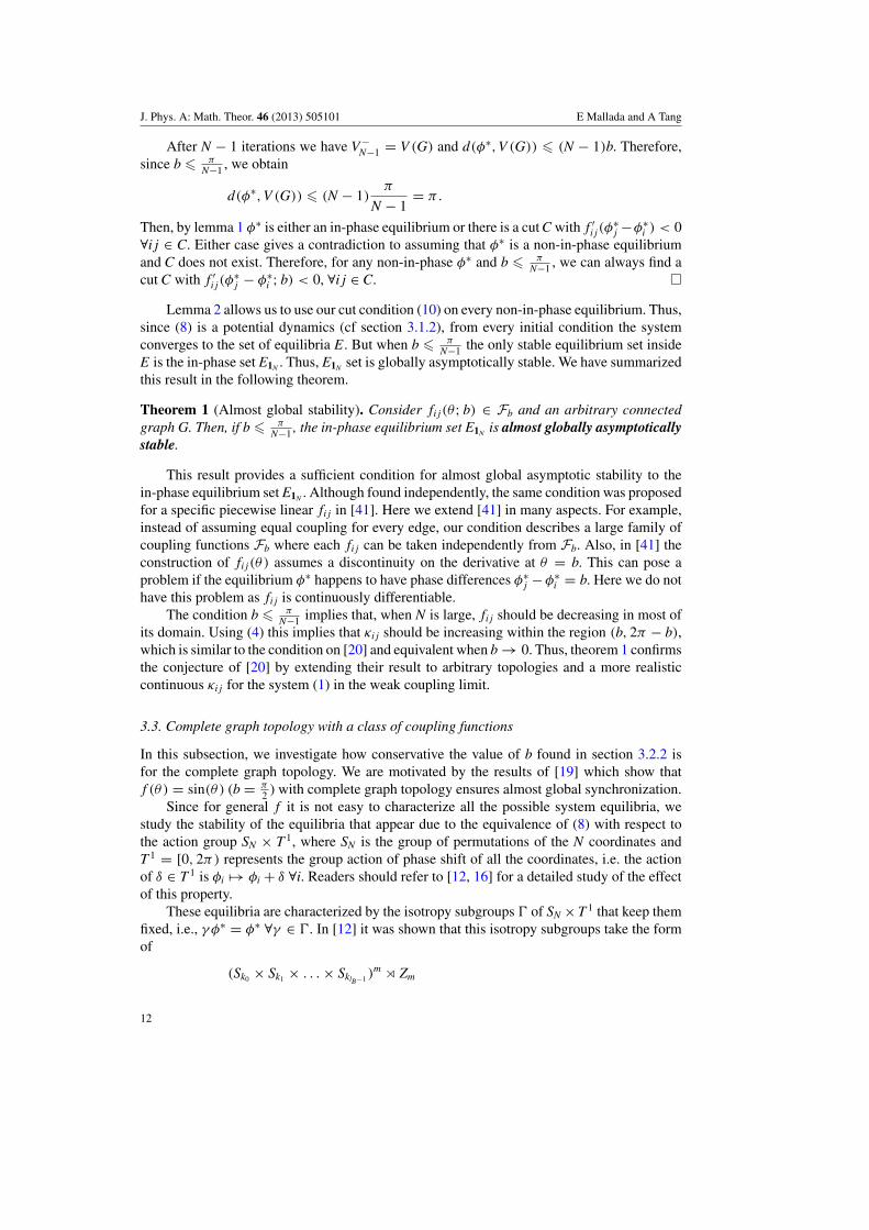
Lemma 2 allows us to use our cut condition (10) on every non-in-phase equilibrium. Thus,since (8) is a potential dynamics (cf section 3.1.2), from every initial condition the systemconverges to the set of equilibria E. But when b � π

N−1 the only stable equilibrium set insideE is the in-phase set E1N . Thus, E1N set is globally asymptotically stable. We have summarizedthis result in the following theorem.

Theorem 1 (Almost global stability). Consider fi j(θ; b) ∈ Fb and an arbitrary connectedgraph G. Then, if b � π

N−1 , the in-phase equilibrium set E1N is almost globally asymptoticallystable.

This result provides a sufficient condition for almost global asymptotic stability to thein-phase equilibrium set E1N . Although found independently, the same condition was proposedfor a specific piecewise linear fi j in [41]. Here we extend [41] in many aspects. For example,instead of assuming equal coupling for every edge, our condition describes a large family ofcoupling functions Fb where each fi j can be taken independently from Fb. Also, in [41] theconstruction of fi j(θ ) assumes a discontinuity on the derivative at θ = b. This can pose aproblem if the equilibrium φ∗ happens to have phase differences φ∗

j −φ∗i = b. Here we do not

have this problem as fi j is continuously differentiable.The condition b � π

N−1 implies that, when N is large, fi j should be decreasing in most ofits domain. Using (4) this implies that κi j should be increasing within the region (b, 2π − b),which is similar to the condition on [20] and equivalent when b → 0. Thus, theorem 1 confirmsthe conjecture of [20] by extending their result to arbitrary topologies and a more realisticcontinuous κi j for the system (1) in the weak coupling limit.

3.3. Complete graph topology with a class of coupling functions

In this subsection, we investigate how conservative the value of b found in section 3.2.2 isfor the complete graph topology. We are motivated by the results of [19] which show thatf (θ ) = sin(θ ) (b = π

2 ) with complete graph topology ensures almost global synchronization.Since for general f it is not easy to characterize all the possible system equilibria, we

study the stability of the equilibria that appear due to the equivalence of (8) with respect tothe action group SN × T 1, where SN is the group of permutations of the N coordinates andT 1 = [0, 2π) represents the group action of phase shift of all the coordinates, i.e. the actionof δ ∈ T 1 is φi �→ φi + δ ∀i. Readers should refer to [12, 16] for a detailed study of the effectof this property.

These equilibria are characterized by the isotropy subgroups � of SN × T 1 that keep themfixed, i.e., γφ∗ = φ∗ ∀γ ∈ �. In [12] it was shown that this isotropy subgroups take the formof

(Sk0 × Sk1 × . . . × SklB−1 )m

� Zm

12

J. Phys. A: Math. Theor. 46 (2013) 505101 E Mallada and A Tang

Figure 6. Equilibria with isotropy (Sk0 × Sk1 × Sk2 )4� Z4 (left) and (Sk )

8� Z8 (right).

where ki and m are positive integers such that (k0+k1+. . .+klB−1)m = N, S j is the permutationsubgroup of SN of j-many coordinates and Zm is the cyclic group with action φi �→ φi + 2π

m .The semi-product � represents the fact that Zm does not commute with the other subgroups.

In other words, each equilibria with isotropy (Sk0 ×Sk1 × . . .×SklB−1 )m

�Zm is conformedby lB shifted constellations Cl (l ∈ {0, 1, . . . lB − 1}) of m evenly distributed blocks, with kl

oscillators per block. We use δl to denote the phase shift between constellation C0 and Cl . Seefigure 6 for examples of these types of equilibria.

Here we will show that under mild assumptions on f and for b = π2 most of the equilibria

found with these characteristics are unstable. We first study all the equilibria with m even. Inthis case, there is a special property that can be exploited.

That is, when f ∈ F π2

such that f is even around π2 , we have

gm(δ) :=m−1∑j=0

f

(2π

mj + δ

)

=m/2−1∑

j=0

f

(2π

mj + δ

)+ f

(π + 2π

mj + δ

)

=m/2−1∑

j=0

f

(2π

mj + δ

)+ f

((3π

2+ 2π

mj + δ

)− π

2

)

=m/2−1∑

j=0

f

(2π

mj + δ

)+ f

(−

(2π

mj + δ

))

=m/2−1∑

j=0

f

(2π

mj + δ

)− f

(2π

mj + δ

)= 0 (15)

where the third step comes from f being even around π/2 and 2π -periodic, and the fourthfrom f being odd.

Having gm(δ) = 0 is the key to prove the instability of every equilibria with even m. Itessentially states that the aggregate effect of one constellation Cl on any oscillator j ∈ V (G)\Cl

is zero when m is even, and therefore any perturbation that maintains Cl has null effect on j.This is shown in the next proposition.

Theorem 2 (Instability for even m). Given an equilibrium φ∗ with isotropy (Sk1 × Sk2 × . . . ×SklB

)m� Zm and f ∈ F π

2even around π

2 . Then, if m is even, φ∗ is unstable.

Proof. We will show the instability of φ∗ by finding a cut of the network satisfying (10). LetV0 ⊂ V (G) be the set of nodes within one of the blocks of the constellation C0 and consider

13

J. Phys. A: Math. Theor. 46 (2013) 505101 E Mallada and A Tang

Figure 7. Cut of theorem 2, the red block represents one possible set V0.

the partition induced by V0 as shown in figure 7, i.e. P = (V0,V (G)\V0). Due to the structureof φ∗, (10) becomes

∑i j∈C(P)

f ′(φ∗j − φ∗

i ) = −k1 f ′(0) +lB∑

l=1

klg′m(δl ),

where g′m(δ) is the derivative of gm and δl is the phase shift between the C0 and Cl . Finally,

since by assumptions gm(δ) ≡ 0 ∀δ it follows that g′m(δ) ≡ 0 and∑

i j∈C(P)

f ′i j(φ

∗j − φ∗

i ) = −k1 f ′(0) < 0.

Therefore, by (10), φ∗ is unstable. �

The natural question that arises is whether similar results can be obtained for m odd. Themain difficulty in this case is that gm(δ) = 0 does not hold since we no longer evaluate f atpoints with phase difference equal to π such that they cancel each other. Therefore, an extramonotonicity condition needs to be added in order to partially answer this question. Theseconditions and their effects are summarized in the following claims.

Lemma 3 (Monotonicity). Given f ∈ F π2

such that f is strictly concave for θ ∈ [0, π ], then

f ′(θ ) − f ′(θ − φ) < 0, 0 � θ − φ < θ � π (16)

f ′(θ ) − f ′(θ + φ) < 0, −π � θ < θ + φ � 0. (17)

Proof. The proof is a direct consequence of the strict concavity of f . Since f (θ ) is strictlyconcave, then basic convex analysis shows that f ′(θ ) is strictly decreasing within [0, π ].Therefore, the inequality (16) follows directly from the fact that θ ∈ [0, π ],θ − φ ∈ [0, π ]and θ − φ < θ . To show (17) it suffices to notice that since f is odd ( f ∈ F π

2), f is strictly

convex in [π, 2π ]. The rest of the proof is analogous to (16). �

Lemma 4 ( f ′ Concavity). Given f ∈ F π2

such that f ′ is strictly concave for θ ∈ [−π2 , π

2 ].Then for all m � 4, f ′( π

m ) � 12 f ′(0).

Proof. Since f ′(θ ) is concave for θ ∈ [−π, π ] then it follows

f ′(π

m

)= f ′

(λm0 + (1 − λm)

π

2

)> λm f ′(0) + (1 − λm) f ′

(π

2

)> λm f ′(0)

14

J. Phys. A: Math. Theor. 46 (2013) 505101 E Mallada and A Tang

Figure 8. Cut used in theorem 3. The dots in red represent all the oscillators of some maximal setS with d(φ∗, S) < 4π

m .

where λm = m−2m . Thus, for m � 4, λm � 1

2 and

f ′(π

m

)>

1

2f ′(0)

as desired. �Now we show the instability of any equilibria with isotropy (Sk1 × Sk2 × . . .× SklB

)m� Zm

for m odd and greater or equal to 7.

Theorem 3 (Instability for m � 7 and odd). Suppose f ∈ F π2

with f concave in [0, π ] andf ′ concave in [−π

2 , π2 ], then for all m = 2k + 1 with k � 3 the equilibria φ∗ with isotropy

(Sk1 × Sk2 × . . . × SklB)m

� Zm are unstable.

Proof. As in theorem 2 we will use our cut condition to show the instability of φ∗. Thus, wedefine a partition P = (S,V (G)\S) of V (G) by taking S to be a maximal subset of V (G) suchthat d(φ, S) < 4π

m , see figure 8 for an illustration of P. Notice that any of these partitions willinclude all the oscillators of two consecutive blocks of every constellation.

Instead of evaluating the total sum of the weights in the cut, we will show that the sumof edge weights of the links connecting the nodes of one constellation in S with the nodesof a possibly different constellation in V (G)\S is negative. In other words, we will focus onshowing ∑

i j∈Kl1 l2

f ′(φ∗j − φ∗

i ) < 0 (18)

where Kl1l2 = {i j : i ∈ Cl1 ∩ S, j ∈ Cl2 ∩ V (G)\S}.Given any subset of integers J, we define

gJm(δ) = gm(δ) −

∑j∈J

f

(2π

mj + δ

).

Then, we can rewrite (18) as∑i j∈Kl1 l2

f ′(φ∗j − φ∗

i ) = (g{0,1}

m

)′(δl1l2 ) + (

g{−1,0}m

)′(δl1l2 )

= 2g′m(δl1l2 ) − f ′

(δl1l2 + 2π

m

)− 2 f ′(δl1l2 ) − f ′

(δl1l2 − 2π

m

)(19)

where δl1l2 ∈ [0, 2πm ] is the phase shift between the two constellations. Then, if we can show

that for all δ ∈ [0, 2πm ] (19) is less than zero, for any values of l1 and l2, (18) will be satisfied.

15

J. Phys. A: Math. Theor. 46 (2013) 505101 E Mallada and A Tang

Since f is odd and even around π2 , f ′ is even and odd around π

2 and g′m(δ) can be rewritten

as

g′m(δ) = f ′(δ) +

∑1�| j|�� k

2 �

{f ′

(δ + 2π

mj

)− f ′

(δ − sgn( j)

π

m+ 2π

mj

)}

−[

f ′(δ + π

mk)

+ f ′(δ − π

mk)]

1[k odd]

where 1[k odd] is the indicator function of the event [k odd], the sum is over all the integers jwith 1 � | j| � � k

2� and k = m−12 .

The last term only appears when k is odd and in fact it is easy to prove that it is alwaysnegative, as shown in the following calculation:

− f ′(δ + π

mk)

− f ′(δ − π

mk)

= − f ′(π

mk + δ

)− f ′

(π

mk − δ

)= − f ′

(π

2− π

2m+ δ

)− f ′

(π

2− π

2m− δ

)= f ′

(π

2− δ + π

2m

)− f ′

(π

2− δ − π

2m

)= f ′(θ ) − f ′(θ − φ) < 0

where in step one we used the fact of f ′ being even, in step two we used k = m−12 and in step

three we used f ′ being odd around π2 . The last step comes from substituting θ = π

2 − δ + π2m ,

φ = πm and applying lemma 3, since for m � 7 we have 0 � θ − φ < θ � π .

Then it remains to show that the terms of the form f ′(δ + 2πm j) − f ′(δ − sgn( j) π

m + 2πm j)

are negative for all j s.t. 1 � | j| � � k2�. This is indeed true when j is positive since for all

δ ∈ [0, 2πm ] we get

0 � δ − π

m+ 2π

mj < δ + 2π

mj � π, for 1 � j �

⌊k

2

⌋and thus we can apply again lemma 3.

When j is negative, there is one exception in which lemma 3 cannot be used since

−π � δ + 2π

mj < δ + 2π

mj + π

m� 0, ∀δ ∈

[0,

2π

m

]

only holds for −� k2� � j � −2. Thus, the term corresponding to j = −1 cannot be directly

eliminated.Therefore, by keeping only the terms of the sum with j = ±1, g′

m is strictly upper boundedfor all δ ∈ [0, 2π

m ] by

g′m(δ) < f ′(δ) + f ′

(δ − 2π

m

)− f ′

(δ − π

m

)+ f ′

(δ + 2π

m

)− f ′

(δ + π

m

). (20)

Now, substituting (20) in (19) we get∑i j∈Kl1 l2

f ′(φ∗j − φ∗

i ) < f ′(

δ − 2π

m

)− 2 f ′

(δ − π

m

)+ f ′

(δ + 2π

m

)− 2 f ′

(δ + π

m

)

� f ′(

δ − 2π

m

)− 2 f ′

(δ − π

m

)− f ′

(δ + π

m

)

� f ′(

δ − 2π

m

)− 2 f ′

(δ − π

m

)where in the last step we used the fact that for m � 6 and δ ∈ [0, 2π

m ], f ′(δ + πm ) � 0.

16

J. Phys. A: Math. Theor. 46 (2013) 505101 E Mallada and A Tang

Finally, since for δ ∈ [0, 2πm ] f ′(δ − 2π

m ) is strictly increasing and f ′(δ − πm ) achieves its

minimum for δ ∈ {0, 2πm }, then

f ′(

δ − 2π

m

)− 2 f ′

(δ − π

m

)� f ′(0) − 2 f ′

(π

m

)� 0

where the last inequality follows from lemma 4.Therefore, for all m odd greater or equal to 7 we obtain∑

i j∈Kl1 l2

f ′(φ∗j − φ∗

i ) < f ′(0) − 2 f ′(π

m

)� 0

and since this result is independent on the indices l1, l2, then

∑i j∈C(S,V (G)\S)

f ′(φ∗j − φ∗

i ) =lB∑

l1=1

lB∑l2=1

∑i j∈Kl1 l2

f ′(φ∗j − φ∗

i ) < 0

and thus φ∗ is unstable. �

4. Effect of delay

In this section, we study how delay can change the stability in a network of weakly coupledoscillators. Using mean field theory, we construct a non-delayed system with the samecontinuum limit. This allows us to use our instability cut condition as well as other toolsavailable in the literature to study the effect of heterogeneous delays on the system’s behavior.In particular, we show that for Kuramoto oscillators heterogeneous and homogeneous delaysare equivalent, and that large heterogeneous delays can help reach synchronization, which areboth a bit counterintuitive conclusions. Our analysis significantly generalizes previous relatedstudies for general coupling functions [28, 42, 43] and complements the study of Kuramotooscillators in [44, 45] by characterizing the parameters of the delay distribution that define thebehavior of the system when the frequencies are homogeneous.

Once delay is introduced in the system of coupled oscillators, the problem becomesfundamentally harder. For example, for pulse-coupled oscillators, the reception of a pulse nolonger gives accurate information about the relative phase difference �φi j = φ j − φi betweenthe two interacting oscillators. Before, at the exact moment when i received a pulse from j, φ j

was zero and the phase difference was estimated locally by i as �φi j = −φi. However, nowwhen i receives the pulse, the difference becomes �φi j = −φi − ψi j. Therefore, the delaypropagation acts as an error introduced in the phase difference measurement and unless someinformation is known about this error, it is impossible to predict the behavior. Moreover, aswe will see later, slight changes in the distribution can produce nonintuitive behaviors.

We will consider the case where the coupling between oscillators is all to all and identical(Ni = N \{i}, ∀i ∈ N and fi j = f ∀i, j). And assume the phase lags ψi j are randomly andindependently chosen from the same distribution with probability density g(ψ). By lettingN → +∞ and ε → 0 while keeping εN =: ε a constant, (3) becomes

v(φ, t) := ω + ε

∫ π

−π

∫ +∞

0f (σ − φ − ψ)g(ψ)ρ(σ, t) dψ dσ, (21)

where ρ(φ, t) is a time-variant normalized phase distribution that keeps track of the fractionof oscillators with phase φ at time t, and v(φ, t) is the velocity field that expresses the netforce that the whole population applies to a given oscillator with phase φ at time t. Since thenumber of oscillators is preserved at any time, the evolution of ρ(φ, t) is governed by thecontinuity equation

17

J. Phys. A: Math. Theor. 46 (2013) 505101 E Mallada and A Tang

0 0.5 1 1.5 2

0

0.2

0.4

0.6

0.8

1

0 0.5 1 1.5 2−1

−0.5

0

0.5

1

0 0.5 1 1.5 2−1

−0.5

0

0.5

1g

∗f f∗g

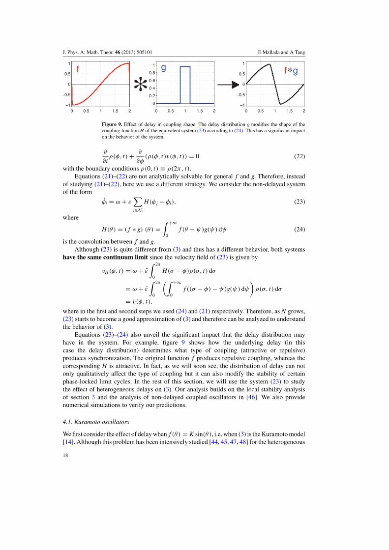
Figure 9. Effect of delay in coupling shape. The delay distribution g modifies the shape of thecoupling function H of the equivalent system (23) according to (24). This has a significant impacton the behavior of the system.

∂

∂tρ(φ, t) + ∂

∂φ(ρ(φ, t)v(φ, t)) = 0 (22)

with the boundary conditions ρ(0, t) ≡ ρ(2π, t).Equations (21)–(22) are not analytically solvable for general f and g. Therefore, instead

of studying (21)–(22), here we use a different strategy. We consider the non-delayed systemof the form

φi = ω + ε∑j∈Ni

H(φ j − φi), (23)

where

H(θ ) = ( f ∗ g) (θ ) =∫ +∞

0f (θ − ψ)g(ψ) dψ (24)

is the convolution between f and g.Although (23) is quite different from (3) and thus has a different behavior, both systems

have the same continuum limit since the velocity field of (23) is given by

vH (φ, t) = ω + ε

∫ 2π

0H(σ − φ)ρ(σ, t) dσ

= ω + ε

∫ 2π

0

(∫ +∞

0f ((σ − φ) − ψ)g(ψ) dψ

)ρ(σ, t) dσ

= v(φ, t),

where in the first and second steps we used (24) and (21) respectively. Therefore, as N grows,(23) starts to become a good approximation of (3) and therefore can be analyzed to understandthe behavior of (3).

Equations (23)–(24) also unveil the significant impact that the delay distribution mayhave in the system. For example, figure 9 shows how the underlying delay (in thiscase the delay distribution) determines what type of coupling (attractive or repulsive)produces synchronization. The original function f produces repulsive coupling, whereas thecorresponding H is attractive. In fact, as we will soon see, the distribution of delay can notonly qualitatively affect the type of coupling but it can also modify the stability of certainphase-locked limit cycles. In the rest of this section, we will use the system (23) to studythe effect of heterogeneous delays on (3). Our analysis builds on the local stability analysisof section 3 and the analysis of non-delayed coupled oscillators in [46]. We also providenumerical simulations to verify our predictions.

4.1. Kuramoto oscillators

We first consider the effect of delay when f (θ ) = K sin(θ ), i.e. when (3) is the Kuramoto model[14]. Although this problem has been intensively studied [44, 45, 47, 48] for the heterogeneous

18

J. Phys. A: Math. Theor. 46 (2013) 505101 E Mallada and A Tang

frequency case using a local stability analysis on (22), our approach unveils new significantimplications. We show that when the frequencies are homogeneous, the Kuramoto model withheterogenous delays can be reduced to the homogeneous delay case with possibly differentcoupling gain. This has been numerically observed in [44] but not theoretically proved.Moreover, we characterize the unique two parameters of the delay distribution that govern theglobal behavior of the system.

We begin by computing (24). When f (θ ) = K sin(θ ), H(θ ) can be easily calculated:

H(θ ) =∫ +∞

0K sin(θ − ψ)g(ψ) dψ

= K∫ +∞

0�[ei(θ−ψ)g(ψ)] dψ = K�

[eiθ

∫ +∞

0e−iψg(ψ) dψ

]= K�[eiθCe−iξ ] = KC sin(θ − ξ )

where � is the imaginary part of a complex number, i.e. �[a + ib] = b. The values of C > 0and ξ are calculated using the identity

Ceiξ =∫ +∞

0eiψg(ψ) dψ. (25)

This complex number, usually called the ‘order parameter’, provides a measure of how thephase lags are distributed within the unit circle. It can also be interpreted as the center of massof the lags ψi j’s when they are thought of as points (eiψi j ) within the unit circle S1. Thus, whenC ≈ 1, the ψi j’s are mostly concentrated around ξ . When C ≈ 0, the delay is distributed suchthat

∑i j eiψi j ≈ 0. Thus, the equivalent non-delayed system (23) becomes

φi = ω + εKC∑j∈Ni

sin(φ j − φi − ξ ). (26)

In other words, when N → +∞ and the natural frequencies are homogeneous, the Kuramotomodel with heterogeneous delays behaves as if the delays were homogenous, with ηi j = ξ

ω∀i j.Furthermore, we can see how the distribution of g(ψ) has a direct effect on the dynamics

through the parametersC and ξ defined in (25). For example, when the delays are heterogeneousenough such that C ≈ 0, the coupling term disappears and therefore makes synchronizationimpossible. A complete study of (26) under the context of superconducting Josephsonarrays was performed in [46]. There the authors characterized the condition for in-phasesynchronization in terms of K and Ceiξ . More precisely, when KCeiξ is on the right half ofthe plane (KC cos(ξ ) > 0), the system almost always synchronizes. However, when KCeiξ ison the left half of the plane (KC cos(ξ ) < 0), the system moves towards an incoherent statewhere all of the oscillators’ phases spread around the unit circle such that its order parameter,i.e. 1

N

∑Nl=1 eiφl ,becomes zero.

We now provide simulation results to illustrate how (26) becomes a good approximationof the original system when N is large enough. We simulate the original repulsive (K < 0)sine-coupled system with heterogeneous delays and its corresponding approximation (26). Twodifferent delay distributions, illustrated in figure 10, were selected such that their correspondingorder parameters lie in different half-planes.

The same simulation is repeated for N = 5, 10, 50. Figure 11 shows that when N is small,the phases’ order parameter of the original system (in red/blue) draws a trajectory which iscompletely different with respect to its approximation (in green). However, as N grows, inboth cases the trajectories become closer and closer. Since K < 0, the trajectory of the systemwith wider distribution (C cos ξ < 0) drives the order parameter towards the boundary of thecircle, i.e., heterogeneous delay leads to homogeneous phase.

19

J. Phys. A: Math. Theor. 46 (2013) 505101 E Mallada and A Tang

Figure 10. Delay distributions and their order parameter Ceiξ .

Figure 11. Repulsive sine coupling with heterogeneous delays: the evolution of the order parameterof the system (3) with K < 0 (repulsive) and delays drawn from the delay distribution of figure 10are shown. The colors match the colors of the corresponding distributions. The green trajectorycorresponds to the non-delayed approximation (26). As N grows the trajectories become closer.

4.2. Effect of heterogeneity

We now explain a more subtle effect that can be produced by heterogeneity. Consider the systemin (23) where H is odd and continuously differentiable. Then, from section 3, all the oscillatorseventually end up running at the same speed ω with fixed phase difference such that the sum∑

i∈NiH(φ j − φi) cancels ∀i. Moreover, we can apply (10) to assess the stability of these

orbits. Therefore, if we can find a cut C of the network such that∑

i j∈C H ′(φ∗j − φ∗

i ) < 0,thephase-locked solution will be unstable.

Although this condition is for non-delayed phase-coupled oscillators, the result of thissection allows us to translate it for systems with delay. Since H is the convolution of thecoupling function f and the delay distribution function g, we can obtain H ′(φ∗

j − φ∗i ) < 0,

even when f ′(φ∗j −φ∗

i ) > 0. This usually occurs when the convolution widens the region witha negative slope of H. See figure 9 for an illustration of this phenomenon.

20

J. Phys. A: Math. Theor. 46 (2013) 505101 E Mallada and A Tang

(a)

(c)

(b)

Figure 12. Pulse-coupled oscillators with delay: stable equilibrium; (a) repulsive coupling f anddelay distribution g; (b) corresponding non-delayed approximation H; (c) oscillators phase snapshotof the system for every time the oscillator number 1 (i = 1) fires.

(a)

(c)

(b)

Figure 13. Pulse-coupled oscillators with delay: unstable equilibrium; (a) repulsive coupling fand delay distribution g; (b) corresponding non-delayed approximation H; (c) oscillators phasesnapshot of the system for every time the oscillator number 1 (i = 1) fires.

Figures 12 and 13 show two simulation setups of 45 oscillators pulse-coupled all to all.The initial state is close to a phase-locked configuration formed by three equidistant clustersof 15 oscillators each. The shape of the coupling function f and the phase lags distribution g

21

J. Phys. A: Math. Theor. 46 (2013) 505101 E Mallada and A Tang

Figure 14. Pulse-coupled oscillators with delay: synchronization probability; each point representthe fraction of times the system with initial condition as in figures 12 and 13 synchronizes in phasefor given standard deviation σ and random chosen delays; the dashed line represents the critical σ

that makes the non-delayed approximation unstable.

are shown in part a; g is a uniform distribution with mean μ = π and variance σ 2. We used (4)to implement the corresponding pulse-coupled system (1). While f is maintained unchangedbetween both simulations, we change the variance, i.e. the heterogeneity, of the distributiong. Thus, the corresponding H = f ∗ g changes as it can be seen in part b; the blue, red andgreen dots correspond to the speed change induced in an oscillator within the blue clusterby oscillators of each cluster. Since all clusters have the same number of oscillators, the neteffect is zero. Part c shows the time evolution of oscillators’ phases relative to the phase of ablue cluster oscillator. Although the initial conditions are exactly the same, the wider delaydistribution on figure 13 produces negative slope on the red and green points of part b, whichdestabilizes the clusters and drives oscillators toward in-phase synchrony.

Finally, we simulate the same scenario as in figures 12 and 13 but now changing N andthe standard deviation, i.e. the delay distribution width. Figure 14 shows the computationof the synchronization probability versus standard deviation of the uniform distributions offigure. The dashed line denotes the minimum value that destabilizes the equivalent system.As N grows, the distribution shape becomes closer to a step, which is the expected shape in

22

J. Phys. A: Math. Theor. 46 (2013) 505101 E Mallada and A Tang

the limit. It is quite surprising that as soon as the equilibrium is within the region of H withnegative slope, the equilibrium becomes unstable as the theory predicts.

5. Conclusion

This paper analyzes the dynamics of identical weakly coupled oscillators while relaxingseveral classical assumptions on coupling, delay and topology. Our results provide globalsynchronization guarantees for a wide range of scenarios. There are many directions thatcan be taken to further this study. For example, for different topologies, to guarantee globalin-phase synchronization, how does the requirement on coupling functions change? Anotherspecific question is to complete the proof in section 3.3 for the cases when m = 1, 3, 5.Finally, it would be of great interest if we could apply results and techniques in this paper toa wide range of applications such as transient stability analysis of power networks and clocksynchronization of computer networks.

Acknowledgments

The authors thank Steven H Strogatz of Cornell for useful discussions.

References

[1] Winfree A T 1967 Biological rhythms and the behavior of populations of coupled oscillators J. Theor.Biol. 16 15–42

[2] Peskin C S 1975 Mathematical Aspects of Heart Physiology (New York: Courant Institute of MathematicalScience)

[3] Achermann P and Kunz H 1999 Modeling circadian rhythm generation in the suprachiasmatic nucleus withlocally coupled self-sustained oscillators: phase shifts and phase response curves J. Biol. Rhythms 14 460–8

[4] Garcia-Ojalvo J, Elowitz M B, Strogatz S H and Peskin C S 2004 Modeling a synthetic multicellular clock:repressilators coupled by quorum sensing Proc. Natl Acad. Sci. USA 101 10955–60

[5] Yamaguchi S, Isejima H, Matsuo T, Okura R, Yagita K, Kobayashi M and Okamura H 2003 Synchronizationof cellular clocks in the suprachiasmatic nucleus Science 32 1408–12

[6] Kiss I Z, Zhai Y and Hudson J L 2002 Emerging coherence in a population of chemical oscillatorsScience 296 1676–8

[7] York R A and Compton R C 1991 Quasi-optical power combining using mutually synchronized oscillator arraysIEEE Trans. Microw. Theory Tech. 39 1000–9

[8] Hong Y-W and Scaglione A 2005 A scalable synchronization protocol for large scale sensor networks and itsapplications IEEE J. Sel. Areas Commun. 23 1085–99

[9] Werner-Allen G, Tewari G, Patel A, Welsh M and Nagpal R 2005 Firefly-inspired sensor network synchronicitywith realistic radio effects SenSys: Proc. of the 3rd Int. Conf. on Embedded Networked Sensor Systems(New York: ACM) pp 142–53

[10] Marvel S A and Strogatz S H 2009 Invariant submanifold for series arrays of Josephson junctionsChaos 19 013132

[11] Bressloff P C and Coombes S 1999 Travelling waves in chains of pulse-coupled integrate-and-fire oscillatorswith distributed delays Physica D 130 232–54

[12] Ashwin P and Swift J W 1992 The dynamics of n weakly coupled identical oscillators J. Nonlinear Sci. 2 69–108[13] Ermentrout G B 1992 Stable periodic solutions to discrete and continuum arrays of weakly coupled nonlinear

oscillators SIAM J. Appl. Math. 52 1665–87[14] Kuramoto Y 1975 International Symposium on Mathematical Problems in Theoretical Physics (Lecture Notes

in Physics vol 39) ed H Arakai (New York: Springer) p 420[15] Popovych O V, Maistrenko Y L and Tass P A 2005 Phase chaos in coupled oscillators Phys. Rev. E 71 065201[16] Brown E, Holmes P and Moehlis J 2003 Globally coupled oscillator networks Perspectives and Problems in

Nonlinear Science: A Celebratory Volume in Honor of Larry Sirovich (New York: Springer) pp 183–215[17] Jadbabaie A, Motee N and Barahona M 2004 On the stability of the Kuramoto model of coupled nonlinear

oscillators Proc. American Control Conf. (Boston, 30 June) vol 5 pp 4296–301

23

J. Phys. A: Math. Theor. 46 (2013) 505101 E Mallada and A Tang

[18] Lucarelli D and Wang I-J 2004 Decentralized synchronization protocols with nearest neighbor communicationProc. 2nd Int. Conf. on Embedded Networked Sensor Systems pp 62–8

[19] Monzon P and Paganini F 2005 Global considerations on the Kuramoto model of sinusoidally coupled oscillatorsProc. 44th IEEE Conf. on Decision and Control, and European Control Conf. (Sevilla, Spain, December1985) pp 3923–8

[20] Mirollo R E and Strogatz S H 1990 Synchronization of pulse-coupled biological oscillators SIAM J. Appl.Math. 50 1645–62

[21] Moreau L 2004 Stability of continuous-time distributed consensus algorithms 43rd IEEE Conf. on Decision andControl vol 4 pp 3998–4003

[22] Ren W and Beard R W 2004 Consensus of information under dynamically changing interaction topologiesProc. 2004 American Control Conf. (30 June–2 July) vol 6 pp 4939–44

[23] Stan G-B and Sepulchre R 2003 Dissipativity characterization of a class of oscillators and networks of oscillatorsProc. 42nd IEEE Conf. on Decision and Control (December) vol 4 pp 4169–73

[24] Scardovi L, Sarlette A and Sepulchre R 2007 Synchronization and balancing on the n-torus Syst. ControlLett. 56 335–41

[25] Sepulchre R, Paley D A and Leonard N E 2008 Stabilization of planar collective motion with limitedcommunication IEEE Trans. Autom. Control 53 706–19

[26] Papachristodoulou A and Jadbabaie A 2006 Synchonization in oscillator networks with heterogeneous delays,switching topologies and nonlinear dynamics Proc. 45th IEEE Conf. on Decision and Control pp 4307–12

[27] Izhikevich E M 1998 Phase models with explicit time delays Phys. Rev. E 58 905–8[28] Izhikevich E M 1999 Weakly pulse-coupled oscillators, fm interactions, synchronization, and oscillatory

associative memory IEEE Trans. Neural Netw. 10 508–26[29] Mallada E and Tang A 2010 Synchronization of phase-coupled oscillators with arbitrary topology Proc.

American Control Conf. pp 1777–82[30] Mallada E and Tang A 2010 Weakly pulse-coupled oscillators: heterogeneous delays lead to homogeneous

phase Proc. 49th IEEE Conf. on Decision and Control pp 992–7[31] Ernst U, Pawelzik K and Geisel T 1995 Synchronization induced by temporal delays in pulse-coupled oscillators

Phys. Rev. Lett. 74 1570–3[32] Ernst U, Pawelzik K and Geisel T 1998 Delay-induced multistable synchronization of biological oscillators

Phys. Rev. E 57 2150–62[33] Kuramoto Y 1984 Chemical Oscillations, Waves, and Turbulence (Berlin: Springer)[34] Sepulchre R, Paley D A and Leonard N E 2007 Stabilization of planar collective motion: all-to-all

communication IEEE Trans. Autom. Control 52 811–24[35] Daido H 1992 Quasientrainment and slow relaxation in a population of oscillators with random and frustrated

interactions Phys. Rev. Lett. 68 1073–6[36] Rantzer A 2001 A dual to Lyapunov’s stability theorem Syst. Control Lett. 42 161–8[37] Bollobas B 1998 Modern Graph Theory (New York: Springer)[38] Godsil C and Royle G 2001 Algebraic Graph Theory (New York: Springer)[39] Khalil H K 1996 Nonlinear Systems 3rd edn (Englewood Cliffs, NJ: Prentice-Hall)[40] Hoppensteadt F C and Izhikevich E M 1997 Weakly Connected Neural Networks (New York: Springer)[41] Sarlette A 2009 Geometry and symmetries in coordination control PhD Thesis University of Liege, Belgium[42] van Vreeswijk C, Abbott L and Ermentrout G B 1994 When inhibition not excitation synchronizes neural firing

J. Comput. Neurosci. 1 313–21[43] Gerstner W 1996 Rapid phase locking in systems of pulse-coupled oscillators with delays Phys. Rev.

Lett. 76 1755–8[44] Aonishi T and Okada M 2002 Dynamically-coupled oscillators–cooperative behavior via dynamical interaction

arXiv:condmat/0207506[45] Lee W S, Ott E and Antonsen T M 2009 Large coupled oscillator systems with heterogeneous interaction delays

Phys. Rev. Lett. 103 044101[46] Watanabe S and Strogatz S H 1994 Constants of motion for superconducting Josephson arrays Physica

D 74 197–253[47] Sakaguchi H and Kuramoto Y 1986 A soluble active rotator model showing phase transitions via mutual

entertainment Prog. Theor. Phys. 76 576–81[48] Yeung M K S and Strogatz S H 1999 Time delay in the kuramoto model of coupled oscillators Phys. Rev.

Lett. 82 648

24