SYMMETRIC POLYNOMIALS: THE FUNDAMENTAL THEOREM …hatleyj/student_theses/kender.pdfWe will explore some key components of symmetric polynomials, including the elementary symmetric

SYMMETRIC POLYNOMIALS: THE FUNDAMENTAL

THEOREM AND UNIQUENESS

By

Nicholas Kender

∗ ∗ ∗ ∗ ∗ ∗ ∗ ∗ ∗

Submitted in partial fulfillment of the major requirements for

the Department of Mathematics

Union College

November 21st, 2019

ii

ABSTRACT

KENDER Symmetric Polynomials.

Department of Mathematics, November 21st, 2019.

ADVISOR: HATLEY, JEFFREY

We explore the Fundamental Theorem of Symmetric Polynomials (FTSP),

using a classical proof that is streamlined by rigorously proving lemmas and

a corollary prior to tackling the FTSP. This paper provides many examples of

the complex ideas in order to provide more clarity and a deeper understanding

of the FTSP. We also explore the historical uses of symmetric polynomials,

dating as far back as 1782 in Edward Waring’s Meditationes Algebraicæ and

as recently as 2005 with an application of the FTSP on multilevel converters

from Chiasson et al.

iii

ACKNOWLEDGEMENT

I first want to say thank you to my mother and father for bringing me into

this world and being such great role models growing up, and teaching me that

hard work does in fact pay off. To my sisters and brother for always being

there for me. For Papa, who showed me what a man is. But most importantly

I want to thank God for the gifts He has given me and for never giving up on

me.

Finally, thank you to Jeff Hatley, my advisor, for leading me through this

challenging process of writing a mathematics thesis. Yo Jeff, I did it!

iv

Contents

ABSTRACT ii

ACKNOWLEDGEMENT iii

1. History of Symmetric Polynomials 1

1.1. Metitationes Algebraicæ 1

1.2. Symmetric Polynomials and Harmonics 2

2. Symmetric Polynomials 4

2.1. Introduction to Symmetric Polynomials 4

2.2. Elementary Symmetric Polynomials 6

2.3. Lexicographic Order and Leading Terms 9

2.4. Leading Terms are the Best! 11

3. Fundamental Theorem of Symmetric Polynomials 18

3.1. FTSP:PSTF (Fundamental Theorem of Symmetric Polynomials:

Please Sit-down, Think-hard, and Focus) 18

3.2. A Symmetric Polynomial is Like a Snowflake 21

4. Cheeseburgers 24

References 26

1

1. History of Symmetric Polynomials

Here we provide a historical context for the study and application of sym-

metric polynomials. We just take a glimpse of the main ideas from previous

sources, but we use the historical context as our motivation to prove the Fun-

damental Theorem of Symmetric Polynomials.

The first time we see symmetric polynomials dates back to 1629, when Al-

bert Girard published his book New Inventions in Algebra, where he provided

a clear description on the elementary symmetric polynomials. Next in the

early 1700’s, Isaac Newton published his work on what are now known as the

Newton Identities ; we explore this concept in Example (2.8) below.

In this paper, we explore two very different uses of symmetric polynomials;

first, we see how Edward Waring defines the idea of the elementary symmetric

polynomials Meditationes Algebraicæ[1] and then we land in 2005 and see an

electrical engineering application of symmetric polynomials.

I hope your flux capacitor is pumping out 1.21 gigawatts, because we are

going on a voyage through time.

1.1. Metitationes Algebraicæ. In the first chapter of Edward Waring’s

1782 book Meditationes Algebraicæ, Waring utilizes what we will prove later

in this paper; the idea that a symmetric polynomial can be written in terms

of the elementary symmetric polynomials. While we see a formal definition of

these concepts in the pages below, first we will consider how Waring applied

symmetric polynomials in Meditationes Algebraicæ.

Suppose α, β, γ, δ, ε, etc. are the roots of a given equation

xn − pxn−1 + qxn−2 − rxn−3 + ... = 0,

2

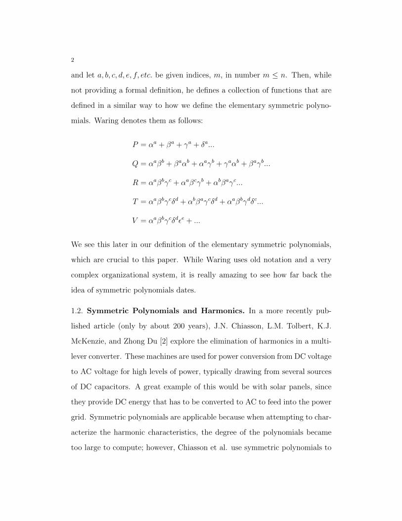
and let a, b, c, d, e, f, etc. be given indices, m, in number m ≤ n. Then, while

not providing a formal definition, he defines a collection of functions that are

defined in a similar way to how we define the elementary symmetric polyno-

mials. Waring denotes them as follows:

P = αa + βa + γa + δa...

Q = αaβb + βaαb + αaγb + γaαb + βaγb...

R = αaβbγc + αaβcγb + αbβaγc...

T = αaβbγcδd + αbβaγcδd + αaβbγdδc...

V = αaβbγcδdεe + ...

We see this later in our definition of the elementary symmetric polynomials,

which are crucial to this paper. While Waring uses old notation and a very

complex organizational system, it is really amazing to see how far back the

idea of symmetric polynomials dates.

1.2. Symmetric Polynomials and Harmonics. In a more recently pub-

lished article (only by about 200 years), J.N. Chiasson, L.M. Tolbert, K.J.

McKenzie, and Zhong Du [2] explore the elimination of harmonics in a multi-

lever converter. These machines are used for power conversion from DC voltage

to AC voltage for high levels of power, typically drawing from several sources

of DC capacitors. A great example of this would be with solar panels, since

they provide DC energy that has to be converted to AC to feed into the power

grid. Symmetric polynomials are applicable because when attempting to char-

acterize the harmonic characteristics, the degree of the polynomials became

too large to compute; however, Chiasson et al. use symmetric polynomials to

3

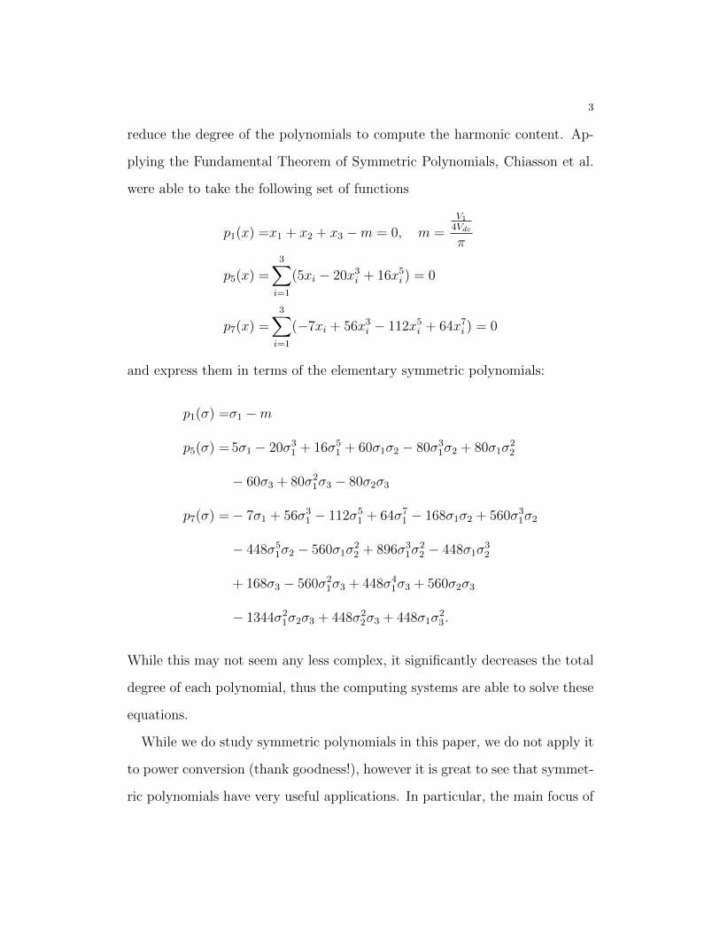
reduce the degree of the polynomials to compute the harmonic content. Ap-

plying the Fundamental Theorem of Symmetric Polynomials, Chiasson et al.

were able to take the following set of functions

p1(x) =x1 + x2 + x3 −m = 0, m =

V14Vdc

π

p5(x) =3∑i=1

(5xi − 20x3i + 16x5i ) = 0

p7(x) =3∑i=1

(−7xi + 56x3i − 112x5i + 64x7i ) = 0

and express them in terms of the elementary symmetric polynomials:

p1(σ) =σ1 −m

p5(σ) = 5σ1 − 20σ31 + 16σ5

1 + 60σ1σ2 − 80σ31σ2 + 80σ1σ

22

− 60σ3 + 80σ21σ3 − 80σ2σ3

p7(σ) =− 7σ1 + 56σ31 − 112σ5

1 + 64σ71 − 168σ1σ2 + 560σ3

1σ2

− 448σ51σ2 − 560σ1σ

22 + 896σ3

1σ22 − 448σ1σ

32

+ 168σ3 − 560σ21σ3 + 448σ4

1σ3 + 560σ2σ3

− 1344σ21σ2σ3 + 448σ2

2σ3 + 448σ1σ23.

While this may not seem any less complex, it significantly decreases the total

degree of each polynomial, thus the computing systems are able to solve these

equations.

While we do study symmetric polynomials in this paper, we do not apply it

to power conversion (thank goodness!), however it is great to see that symmet-

ric polynomials have very useful applications. In particular, the main focus of

4

this paper, the Fundamental Theorem of Symmetric Polynomials, is relevant

in electrical engineering and beyond!

2. Symmetric Polynomials

2.1. Introduction to Symmetric Polynomials. Symmetric polynomials

are exactly what the name suggests; put in layman’s terms, if any of the

variables in a polynomial are interchanged, then we get the same polynomial.

We will explore some key components of symmetric polynomials, including the

elementary symmetric polynomials, which have some very useful applications.

We start out by giving a formal definition of symmetric polynomials, and then

there are some examples to help fully understand the concept.

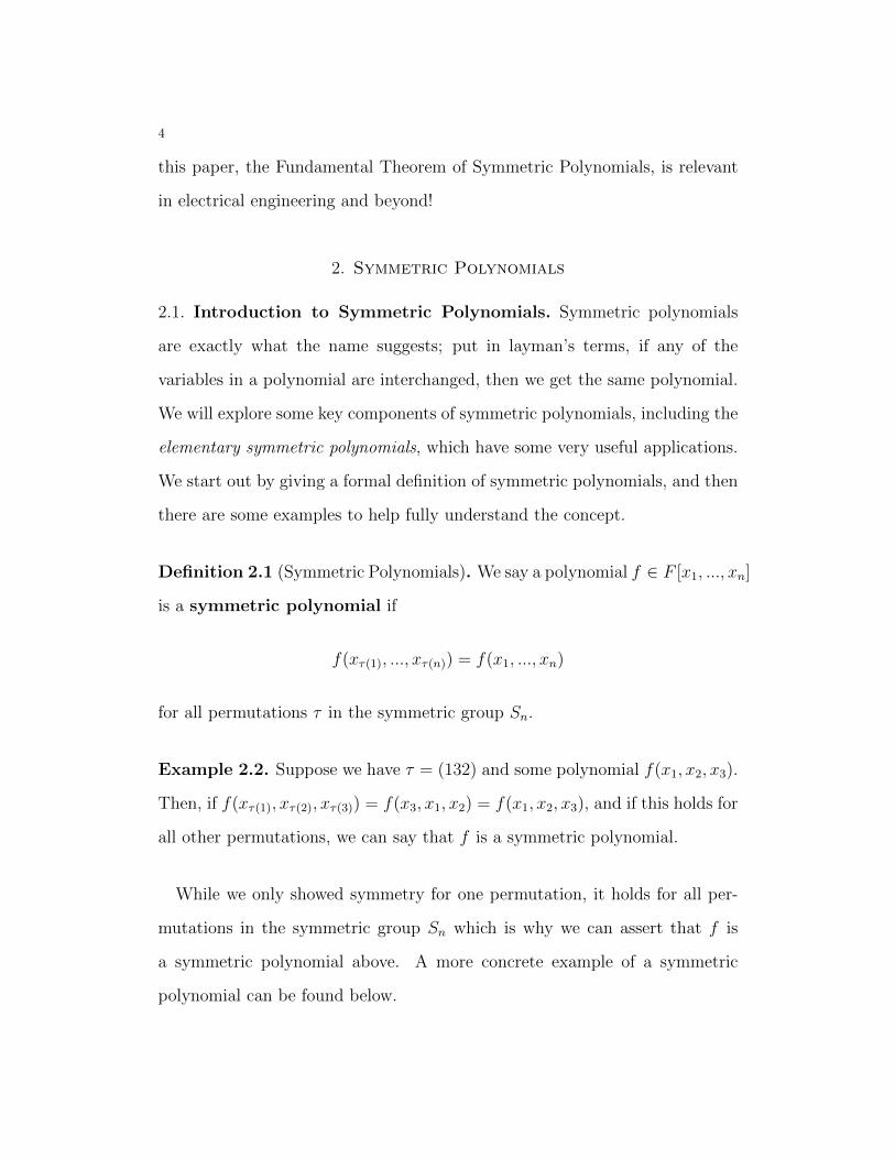
Definition 2.1 (Symmetric Polynomials). We say a polynomial f ∈ F [x1, ..., xn]

is a symmetric polynomial if

f(xτ(1), ..., xτ(n)) = f(x1, ..., xn)

for all permutations τ in the symmetric group Sn.

Example 2.2. Suppose we have τ = (132) and some polynomial f(x1, x2, x3).

Then, if f(xτ(1), xτ(2), xτ(3)) = f(x3, x1, x2) = f(x1, x2, x3), and if this holds for

all other permutations, we can say that f is a symmetric polynomial.

While we only showed symmetry for one permutation, it holds for all per-

mutations in the symmetric group Sn which is why we can assert that f is

a symmetric polynomial above. A more concrete example of a symmetric

polynomial can be found below.

5

Example 2.3. Suppose we have a polynomial f such that f = 2x1 · x2 · x3 +

2x1 · x3 + 2x1 · x2 + 2x2 · x3. Since we can interchange any of the xi, we say

that this is a symmetric polynomial.

To solidify our understanding of what a symmetric polynomial really is, we

will consider the following non-example.

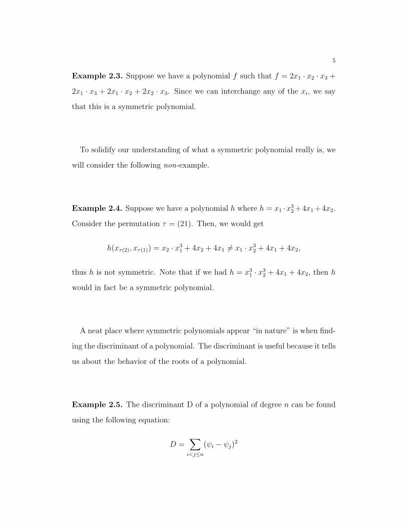
Example 2.4. Suppose we have a polynomial h where h = x1 ·x32 +4x1 +4x2.

Consider the permutation τ = (21). Then, we would get

h(xτ(2), xτ(1)) = x2 · x31 + 4x2 + 4x1 6= x1 · x32 + 4x1 + 4x2,

thus h is not symmetric. Note that if we had h = x31 · x32 + 4x1 + 4x2, then h

would in fact be a symmetric polynomial.

A neat place where symmetric polynomials appear “in nature” is when find-

ing the discriminant of a polynomial. The discriminant is useful because it tells

us about the behavior of the roots of a polynomial.

Example 2.5. The discriminant D of a polynomial of degree n can be found

using the following equation:

D =∑i<j≤n

(ψi − ψj)2

6

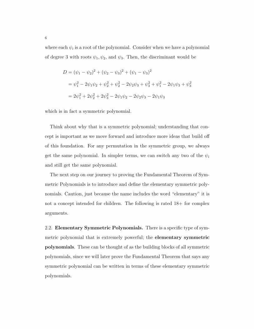
where each ψi is a root of the polynomial. Consider when we have a polynomial

of degree 3 with roots ψ1, ψ2, and ψ3. Then, the discriminant would be

D = (ψ1 − ψ2)2 + (ψ2 − ψ3)

2 + (ψ1 − ψ3)2

= ψ21 − 2ψ1ψ2 + ψ2

2 + ψ22 − 2ψ2ψ3 + ψ2

3 + ψ21 − 2ψ1ψ3 + ψ2

3

= 2ψ21 + 2ψ2

2 + 2ψ23 − 2ψ1ψ2 − 2ψ2ψ3 − 2ψ1ψ3

which is in fact a symmetric polynomial.

Think about why that is a symmetric polynomial; understanding that con-

cept is important as we move forward and introduce more ideas that build off

of this foundation. For any permutation in the symmetric group, we always

get the same polynomial. In simpler terms, we can switch any two of the ψi

and still get the same polynomial.

The next step on our journey to proving the Fundamental Theorem of Sym-

metric Polynomials is to introduce and define the elementary symmetric poly-

nomials. Caution, just because the name includes the word “elementary” it is

not a concept intended for children. The following is rated 18+ for complex

arguments.

2.2. Elementary Symmetric Polynomials. There is a specific type of sym-

metric polynomial that is extremely powerful; the elementary symmetric

polynomials. These can be thought of as the building blocks of all symmetric

polynomials, since we will later prove the Fundamental Theorem that says any

symmetric polynomial can be written in terms of these elementary symmetric

polynomials.

7

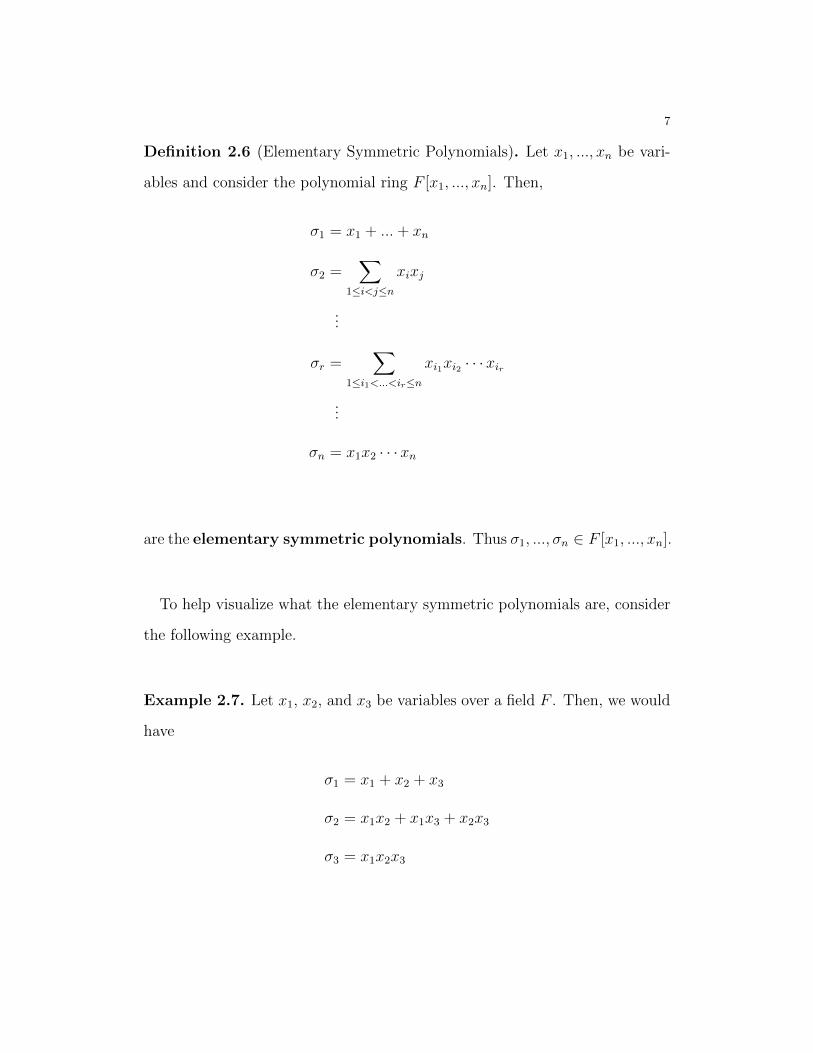
Definition 2.6 (Elementary Symmetric Polynomials). Let x1, ..., xn be vari-

ables and consider the polynomial ring F [x1, ..., xn]. Then,

σ1 = x1 + ...+ xn

σ2 =∑

1≤i<j≤n

xixj

...

σr =∑

1≤i1<...<ir≤n

xi1xi2 · · · xir

...

σn = x1x2 · · ·xn

are the elementary symmetric polynomials. Thus σ1, ..., σn ∈ F [x1, ..., xn].

To help visualize what the elementary symmetric polynomials are, consider

the following example.

Example 2.7. Let x1, x2, and x3 be variables over a field F . Then, we would

have

σ1 = x1 + x2 + x3

σ2 = x1x2 + x1x3 + x2x3

σ3 = x1x2x3

8

Due to the commutative property of addition and multiplication, we can per-

mute σ1 and σ3 in any way and still get the same outcome, thus they are

symmetric. It is less obvious that σ2 is symmetric, but rest assured, it is;

consider the permutation τ = (132). We would get

σ2 = x3x1 + x3x2 + x1x2,

which is equivalent to the original. A similar argument can be used for other

permutations to show that the above polynomials are in fact symmetric.

Now we are certain that the elementary symmetric polynomials are, well,

symmetric. Never trust a book by its cover, and never trust a math concept

by its name.

As promised, we will now explore a classical example that comes from Isaac

Newton’s book Arithmetica universalis, published in 1707. The Newton Iden-

tities show the relationship between power sums and elementary symmetric

polynomials, so we first must see what the power sums are.

Example 2.8 (Newton Identities). Albert Girard is credited with publishing

the first power sums in 1629, which he defined as

sr = xr1 + · · ·+ xrn

When r = 1 we get σ1, and when r > 1 we get the Newton identities :

sr = σ1sr−1 − σ2sr−2 + . . .+ (−1)r−1rσr if 1 < r ≤ n,

sr = σ1sr−1 − σ2sr−2 + . . .+ (−1)r−1σnsr−n if r > n.

9

This is a neat example to consider that symmetric polynomials have been

thought about since the 1600s. At this point, I am pretty much Isaac Newton’s

apprentice.

Now that we have a firm grasp of what a symmetric polynomial looks like

and what the elementary symmetric polynomials are, we look forward to the

Fundamental Theorem of Symmetric Polynomials (FTSP) which states that

any symmetric polynomial in F [x1, ..., xn] can be written in terms of σ1, ..., σn.

However, before we consider the FTSP, we must first state a few definitions,

prove a few lemmas, and dare we forget to introduce and prove a corollary!

2.3. Lexicographic Order and Leading Terms. The proof of the FTSP in-

volves an inductive process which requires that we order monomials xa11 · · ·xannin x1, ..., xn. We will use graded lexicographic order.

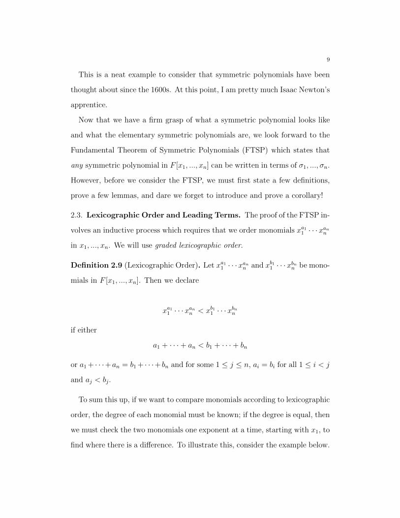
Definition 2.9 (Lexicographic Order). Let xa11 · · ·xann and xb11 · · ·xbnn be mono-

mials in F [x1, ..., xn]. Then we declare

xa11 · · ·xann < xb11 · · ·xbnn

if either

a1 + · · ·+ an < b1 + · · ·+ bn

or a1 + · · ·+an = b1 + · · ·+ bn and for some 1 ≤ j ≤ n, ai = bi for all 1 ≤ i < j

and aj < bj.

To sum this up, if we want to compare monomials according to lexicographic

order, the degree of each monomial must be known; if the degree is equal, then

we must check the two monomials one exponent at a time, starting with x1, to

find where there is a difference. To illustrate this, consider the example below.

10

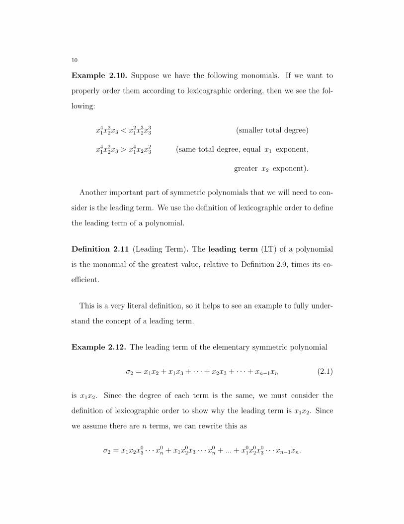
Example 2.10. Suppose we have the following monomials. If we want to

properly order them according to lexicographic ordering, then we see the fol-

lowing:

x41x22x3 < x21x

32x

33 (smaller total degree)

x41x22x3 > x41x2x

23 (same total degree, equal x1 exponent,

greater x2 exponent).

Another important part of symmetric polynomials that we will need to con-

sider is the leading term. We use the definition of lexicographic order to define

the leading term of a polynomial.

Definition 2.11 (Leading Term). The leading term (LT) of a polynomial

is the monomial of the greatest value, relative to Definition 2.9, times its co-

efficient.

This is a very literal definition, so it helps to see an example to fully under-

stand the concept of a leading term.

Example 2.12. The leading term of the elementary symmetric polynomial

σ2 = x1x2 + x1x3 + · · ·+ x2x3 + · · ·+ xn−1xn (2.1)

is x1x2. Since the degree of each term is the same, we must consider the

definition of lexicographic order to show why the leading term is x1x2. Since

we assume there are n terms, we can rewrite this as

σ2 = x1x2x03 · · ·x0n + x1x

02x3 · · · x0n + ...+ x01x

02x

03 · · ·xn−1xn.

11

Thus, when we apply lexicographic order to find the leading term, it becomes

clear that x1x2 is in fact the leading term; comparing the first two terms, since

the first term = x1x2 and the second term = x1x02x3, clearly x2 has a bigger

exponent value than x02, thus the first term is bigger than the second term. A

similar argument shows why x1x2 is bigger than any other term, thus x1x2 is

the leading term of σr.

We now have a good understanding on the make-up of symmetric polyno-

mials, so now we will begin to take a deeper dive into understanding them and

prove a few lemmas and a corollary to help us with the proof of the FTSP.

2.4. Leading Terms are the Best! We need the following lemmas and corol-

lary in order to provide a rigorous proof of the FTSP. They focus on the useful-

ness of the leading term of a symmetric polynomial as well as the combination

of multiple symmetric polynomials.

Lemma 2.13. Let f, g ∈ F [x1, ..., xn] be nonzero. Then, LT(fg) = LT(f)LT(g).

Proof. Let x = x1 · · ·xn be a monomial in F [x1, ..., xn] and let α = (a1, ..., an),

β = (b1, ..., bn), ρ = (r1, ..., rn), and δ = (d1, ..., dn) be exponent vectors where

every ai, bi, ri, and di are non-negative integers. Then, xα = xa11 · · ·xann ,

xβ = xb11 · · ·xbnn , xρ = xr11 · · ·xrnn , and xδ = xd11 · · ·xdnn . Suppose xα > xβ and

let xρ be any monomial. Consider xαxρ and xβxρ. We see that

xαxρ = xa11 xr11 · · · xann xrnn

= xa1+r1 · · ·xan+rn

= xα+ρ.

12

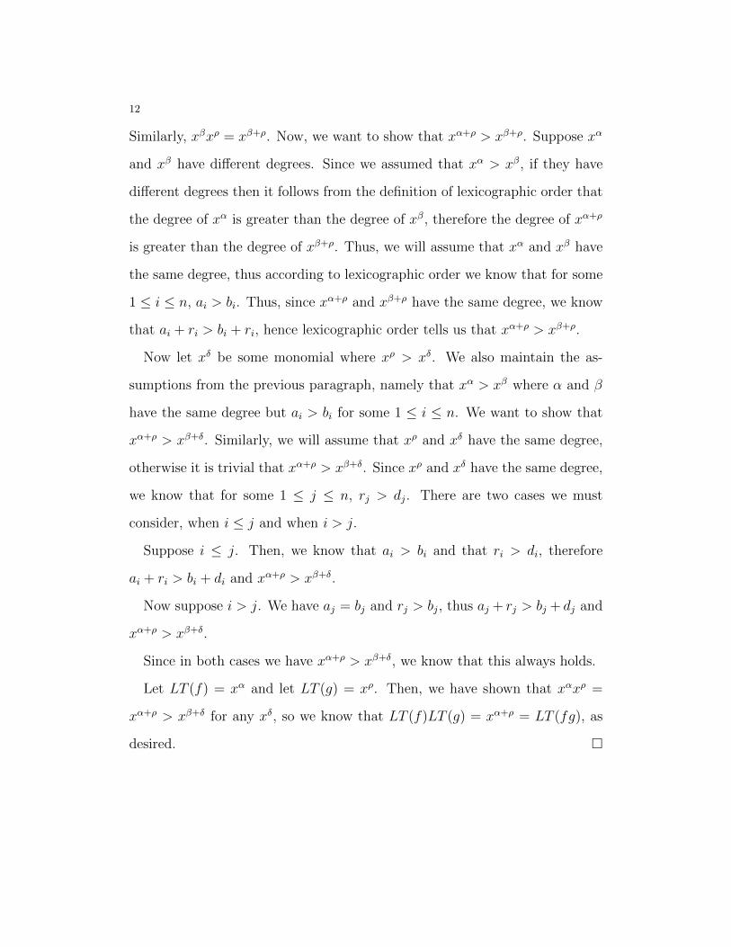
Similarly, xβxρ = xβ+ρ. Now, we want to show that xα+ρ > xβ+ρ. Suppose xα

and xβ have different degrees. Since we assumed that xα > xβ, if they have

different degrees then it follows from the definition of lexicographic order that

the degree of xα is greater than the degree of xβ, therefore the degree of xα+ρ

is greater than the degree of xβ+ρ. Thus, we will assume that xα and xβ have

the same degree, thus according to lexicographic order we know that for some

1 ≤ i ≤ n, ai > bi. Thus, since xα+ρ and xβ+ρ have the same degree, we know

that ai + ri > bi + ri, hence lexicographic order tells us that xα+ρ > xβ+ρ.

Now let xδ be some monomial where xρ > xδ. We also maintain the as-

sumptions from the previous paragraph, namely that xα > xβ where α and β

have the same degree but ai > bi for some 1 ≤ i ≤ n. We want to show that

xα+ρ > xβ+δ. Similarly, we will assume that xρ and xδ have the same degree,

otherwise it is trivial that xα+ρ > xβ+δ. Since xρ and xδ have the same degree,

we know that for some 1 ≤ j ≤ n, rj > dj. There are two cases we must

consider, when i ≤ j and when i > j.

Suppose i ≤ j. Then, we know that ai > bi and that ri > di, therefore

ai + ri > bi + di and xα+ρ > xβ+δ.

Now suppose i > j. We have aj = bj and rj > bj, thus aj + rj > bj + dj and

xα+ρ > xβ+δ.

Since in both cases we have xα+ρ > xβ+δ, we know that this always holds.

Let LT (f) = xα and let LT (g) = xρ. Then, we have shown that xαxρ =

xα+ρ > xβ+δ for any xδ, so we know that LT (f)LT (g) = xα+ρ = LT (fg), as

desired. �

13

Understanding what happens to the leading terms of two symmetric polyno-

mials when we multiply them together is a crucial part of proving the FTSP.

Thus, we will highlight an example to get a more concrete understanding.

Example 2.14. Suppose we have the following symmetric polynomials

f = x21x22 + x21 + x22

g = 7x1x2x3 + x1 + x2 + x3.

According to lexicographic order, we know that LT (f) = x21x22 and LT (g) =

7x1x2x3. We want to show that LT (f · g) = 7x31x32x3. We see that

f · g =7x31x32x3 + x31x

22 + x21x

32 + x21x

22x3 + 7x31x2x3+

x31 + x21x2 + x21x3 + 7x1x32x3 + x1x

22 + x32 + x22x3

The only monomial in f · g of degree 7 is 7x31x32x3 and every other term has a

lower degree, thus it is the leading term. So, LT (f) · LT (g) = LT (f · g), as

desired.

The leading term of a symmetric polynomial is very helpful information; so,

it makes sense to be curious what the leading term of the elementary symmetric

polynomials looks like. Well, fear not because the next lemma illustrates that

exactly.

Lemma 2.15. Suppose σr is some nonzero elementary symmetric polynomial.

Then, LT (σr) = x1x2 · · ·xr.

Proof. Consider σr = x1x2x3 · · ·xr+x1x3 · · · xrxr+1+x1x2 · · ·xrxr+1xr+2+...+

x1x2 · · ·xn. We know that each term has the same degree, so we must compare

14

the exponent values according to lexicographic order to determine which term

is the leading term. Similar to Example (2.12), we know that the first term is

greater than the second term because σr1 = x1x2x3 · · ·xr has degree 1 for x2

and σr2 = x1x3 · · ·xrxr+1 has degree 0 for x2. A similar argument shows why

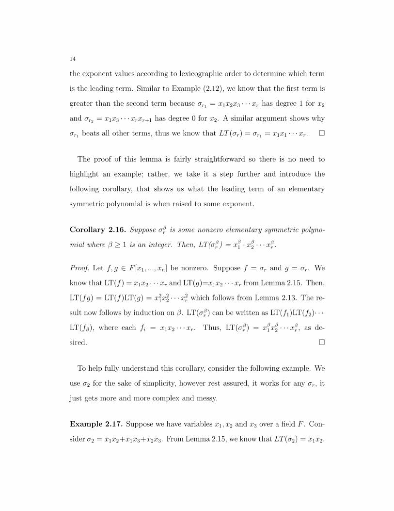
σr1 beats all other terms, thus we know that LT (σr) = σr1 = x1x1 · · ·xr. �

The proof of this lemma is fairly straightforward so there is no need to

highlight an example; rather, we take it a step further and introduce the

following corollary, that shows us what the leading term of an elementary

symmetric polynomial is when raised to some exponent.

Corollary 2.16. Suppose σβr is some nonzero elementary symmetric polyno-

mial where β ≥ 1 is an integer. Then, LT(σβr ) = xβ1 · xβ2 · · ·xβr .

Proof. Let f, g ∈ F [x1, ..., xn] be nonzero. Suppose f = σr and g = σr. We

know that LT(f) = x1x2 · · ·xr and LT(g)=x1x2 · · ·xr from Lemma 2.15. Then,

LT(fg) = LT(f)LT(g) = x21x22 · · · x2r which follows from Lemma 2.13. The re-

sult now follows by induction on β. LT(σβr ) can be written as LT(f1)LT(f2)· · ·

LT(fβ), where each fi = x1x2 · · ·xr. Thus, LT(σβr ) = xβ1xβ2 · · ·xβr , as de-

sired. �

To help fully understand this corollary, consider the following example. We

use σ2 for the sake of simplicity, however rest assured, it works for any σr, it

just gets more and more complex and messy.

Example 2.17. Suppose we have variables x1, x2 and x3 over a field F . Con-

sider σ2 = x1x2+x1x3+x2x3. From Lemma 2.15, we know that LT (σ2) = x1x2.

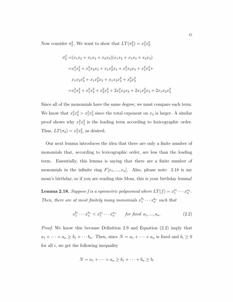
15

Now consider σ22. We want to show that LT (σ2

2) = x21x22.

σ22 =(x1x2 + x1x3 + x2x3)(x1x2 + x1x3 + x2x3)

=x21x22 + x21x2x3 + x1x

22x3 + x21x2x3 + x21x

23+

x1x2x23 + x1x

22x3 + x1x2x

23 + x22x

23

=x21x22 + x21x

23 + x22x

23 + 2x21x2x3 + 2x1x

22x3 + 2x1x2x

23

Since all of the monomials have the same degree, we must compare each term.

We know that x21x22 > x21x

23 since the total exponent on x2 is larger. A similar

proof shows why x21x22 is the leading term according to lexicographic order.

Thus, LT (σ2) = x21x22, as desired.

Our next lemma introduces the idea that there are only a finite number of

monomials that, according to lexicographic order, are less than the leading

term. Essentially, this lemma is saying that there are a finite number of

monomials in the infinite ring F [x1, ..., xn]. Also, please note: 2.18 is my

mom’s birthday, so if you are reading this Mom, this is your birthday lemma!

Lemma 2.18. Suppose f is a symmetric polynomial where LT (f) = xa11 · · ·xann .

Then, there are at most finitely many monomials xb11 · · ·xbnn such that

xb11 · · · xbnn < xa11 · · · xann for fixed a1, ..., an. (2.2)

Proof. We know this because Definition 2.9 and Equation (2.2) imply that

a1 + · · · + an ≥ b1 + · · · bn. Then, since N = a1 + · · · + an is fixed and bi ≥ 0

for all i, we get the following inequality

N = a1 + · · ·+ an ≥ b1 + · · ·+ bn ≥ bi

16

for all i. This tells us that there are only N+1 possibilities for each bi, implying

that (2.2) can hold for at most finitely many xb11 · · ·xbnn . �

Since this lemma is more fundamental, we will not be going through an

example of it; however, it still is an important thing to keep in mind once

we begin considering the FTSP. Our penultimate lemma deals with the lin-

ear combinations of two symmetric polynomials and states that if you add

them together, even if one is multiplied by a constant integer, the resulting

polynomial is also symmetric.

Lemma 2.19. Suppose f and g are symmetric polynomials and c is some

constant integer. Then, f + cg is also a symmetric polynomial.

Proof. Assume f and g are both symmetric. By definition, we know that

f(xτ ) = f(x) and g(xτ ) = g(x) where τ is some permutation of f . Let c ∈ Z

be some constant. We know that cg(x) = c[g(x)]. Then, we know that

(f + cg)(x) = f(x) + cg(x).

But, since both f and cg are symmetric, we also know that

(f + cg)(xτ ) = f(xτ ) + c[g(xτ )] = f(x) + c[g(x)] = (f + cg)(x),

so by definition this is symmetric. �

We see a nice example of this lemma in action below.

Example 2.20. Suppose f = x1 +x2 and g = x1x2 and c = 2. We can clearly

see that both f and g are symmetric; thus, Lemma 2.19 tells us that f + cg

17

must also be symmetric. We see that

f + cg = x1 + x2 + 2x1x2,

which is symmetric, as desired.

If you have made it this far, I am very thankful. It means a lot that you are

willing to read my work, and I promise that the end is near. Just one more

lemma and then we really get into the exciting parts, proving the Fundamental

Theorem of Symmetric Polynomials- that just sounds awesome, right?

Our last lemma that we need is helping us to understand what the leading

term of a symmetric polynomial actually looks like. This is powerful informa-

tion, so use it wisely.

Lemma 2.21. Let f ∈ F [x1, ..., xn] be symmetric with some nonzero leading

term cxa11 · · ·xann . Then, a1 ≥ a2 ≥ · · · ≥ an

Proof. By way of contradiction, suppose that ai < ai+1 for some 1 ≤ i ≤

n − 1. By definition of the leading term, we know that there does not exist

a monomial that has a greater degree than cxa11 · · · xann . Due to Definition

(2.9), we do not have to consider any monomial of lower degree since it would

automatically be disqualified. Thus, we only have to consider monomials of

the same degree as cxa11 · · ·xann . Since f is a symmetric polynomial, we can

permute it and maintain the same polynomial. So, we will switch xi and

xi+1. Then, we have a new monomial in f , namely cxa11 · · ·xaii+1x

ai+1

i · · ·xann .

Based on our assumption that ai < ai+1, by Definition (2.9) we see see that

cxa11 · · ·xaii+1x

ai+1

i · · · xann is a term of f that is greater than cxa11 · · ·xann . This is

because xi has an exponent value of ai in cxa11 · · · xaii · · ·xann and an exponent

18

value of ai+1 in cxa11 · · ·xaii+1x

ai+1

i · · ·xann , and since we assumed that ai+1 > ai,

by Definition (2.9), we know that cxa11 · · ·xaii+1x

ai+1

i · · · xann is a term that is

greater than cxa11 · · ·xann . Yet cxa11 · · ·xann is our leading term, therefore we

have a contradiction, thus ai+1 ≤ ai, as desired. �

Now that we have ventured through the hardware aisles of Home Depot,

we have the necessary tools to tackle the Fundamental Theorem of Symmetric

Polynomials.

3. Fundamental Theorem of Symmetric Polynomials

3.1. FTSP:PSTF (Fundamental Theorem of Symmetric Polynomials:

Please Sit-down, Think-hard, and Focus). Sorry, I could not pass up on

the opportunity for some beautiful symmetry in my section title. Back to

business.

We will be taking a similar approach to proving the FTSP as David Cox in

his book Galois Theory [3], however we have already done most of the leg work

for the proof. A more modern approach to this theorem would be to apply

Galois Theory, however it requires a deeper understanding of group theory and

field theory, which goes beyond the scope of this thesis. Plus, the proof using

Galois Theory is short, so what fun is that? We want a good head-scratcher,

and that is exactly what we are going to get.

Theorem 3.1 (Fundamental Theorem of Symmetric Polynomials). Any sym-

metric polynomial in F [x1, ..., xn] can be written as a polynomial in σ1, ..., σn

with coefficients in F .

19

Proof. Suppose f ∈ F [x1, ..., xn] is a symmetric polynomial where LT (f) =

cxa11 · · ·xann . By Lemma 2.21, we know that a1 ≤ · · · ≤ an.

Now consider

g = σa1−a21 σa2−a32 · · ·σan−1−ann−1 σann . (3.1)

Since we know that each ai ≥ ai+1, we know that this is a polynomial. Then,

by Lemma 2.18 and Corollary 2.16 we know that

LT (g) = xa1−a21 (x1x2)a2−a3(x1x2x3)

a3−a4 · · · (x1 · · ·xn−1)an−a−an(x1 · · ·xn)an

= xa1−a2+a2+a3+...+an1 xa2−a3+...+an2 · · ·xan−1−an+ann−1 xann (3.2)

= xa11 · · ·xann

Thus, we see that LT (cg) = LT (f), so we define f1 = f − cg as a polynomial

with strictly smaller leading term than f due to Definition (2.9), and we know

that f1 is symmetric due to Lemma (2.19).

By a similar method, we can show that there is a f2 = f1−c1g1 with a leading

term strictly smaller than f1. But, we can rewrite this as f2 = f − cg − c1g1.

By continuing this method, we get we get the following polynomials:

f, f1 = f − cg, f2 = f − cg − c1g1, f3 = f − cg − c1g1 − c2g2, ...,

By Lemma (2.18), we know that there is eventually some m such that fm = 0.

Since fm = 0, there is no leading term, therefore the process terminates and

we obtain

f = cg + c1g1 + · · ·+ cm−1gm−1. (3.3)

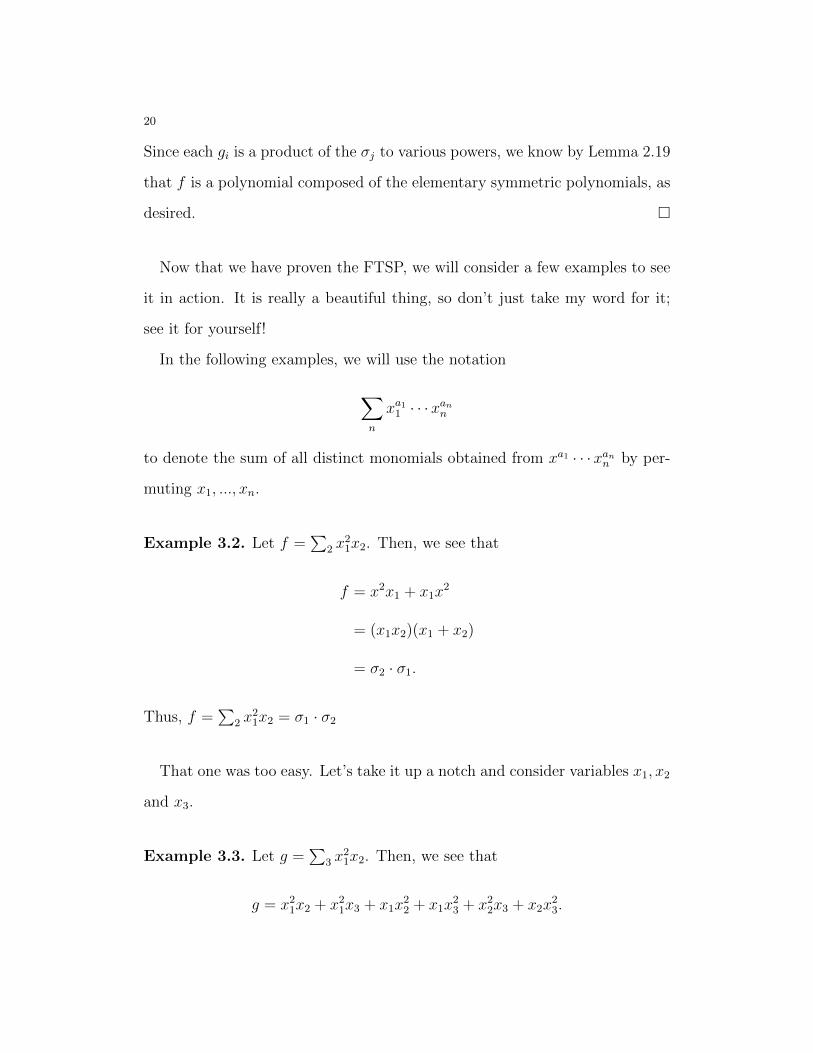
20

Since each gi is a product of the σj to various powers, we know by Lemma 2.19

that f is a polynomial composed of the elementary symmetric polynomials, as

desired. �

Now that we have proven the FTSP, we will consider a few examples to see

it in action. It is really a beautiful thing, so don’t just take my word for it;

see it for yourself!

In the following examples, we will use the notation

∑n

xa11 · · ·xann

to denote the sum of all distinct monomials obtained from xa1 · · ·xann by per-

muting x1, ..., xn.

Example 3.2. Let f =∑

2 x21x2. Then, we see that

f = x2x1 + x1x2

= (x1x2)(x1 + x2)

= σ2 · σ1.

Thus, f =∑

2 x21x2 = σ1 · σ2

That one was too easy. Let’s take it up a notch and consider variables x1, x2

and x3.

Example 3.3. Let g =∑

3 x21x2. Then, we see that

g = x21x2 + x21x3 + x1x22 + x1x

23 + x22x3 + x2x

23.

21

Now consider

(x1 + x2 + x3)(x1x2 + x1x3 + x2x3) = σ1 · σ2 =

= x21x2 + x2x3 + x1x2x3 + x1x22 + x1x2x3 + x22x3 + x1x2x3+

x1x23 + x2x

23

= x21x2 + x2x3 + x1x22 + x22x3 + x1x

23 + x2x

23 + 3x1x2x3

= g + 3x1x2x3

Since 3x1x2x3 = 3 · σ3, we see that g = σ1 · σ2 − 3σ3, thus we have found g in

terms of the elementary symmetric polynomials, as desired.

The final exciting theorem that we explore here takes the FTSP one step

further and says that there is only one way in which we can express a symmetric

polynomial in terms of the elementary symmetric polynomials.

3.2. A Symmetric Polynomial is Like a Snowflake. Indeed, while every

snowflake is unique in shape and pattern, each symmetric polynomial is unique

in that there is only one way to write it in terms of the elementary symmetric

polynomials. Since we know that every symmetric polynomial can be written

in terms of the elementary symmetric polynomials, we now want to assert that

this is unique.

Theorem 3.4. A given symmetric polynomial can be expressed as a polynomial

in the elementary symmetric polynomials in only one way.

Proof. We will use the polynomial ring F [u1, ..., un], where u1, ..., un are new

variables. We know the map sending ui to σi ∈ F [x1, ..., xn] defines a ring

22

homomorphism

φ : F [u1, ..., un]→ F [x1, ..., xn]

In other words, if h = h(u1, ..., un) is a polynomial in u1, ...un with co-

efficients in F , then φ(h) = h(σ1, ..., σn). The image of φ is the set of all

polynomials in the σi with coefficients in F . We denote this image by

Im(φ) = F [σ1, ..., σn] ⊂ F [x1, ..., xn].

Note that F [σ1, ..., σn] is a subring of F [x1, ..., xn]. In this notation, we can

write φ as a map

φ : F [u1, ..., un]→ F [σ1, ..., σn]. (3.4)

This map is onto by the definition of F [σ1, ..., σn], and uniqueness will be

proved by showing that φ is one-to-one. In order to show that φ is one-to-one,

we will show that its kernel is {0}.

Let’s assume h ∈ F [u1, . . . , un] is nonzero. To show uniqueness, we must

show that φ(h) = h(σ1, ..., σn) is not the zero polynomial in x1, ..., xn.

Suppose cub11 · · ·ubnn is a term of h. By applying φ to cub11 · · ·ubnn , we get

cσb11 · · ·σbnn . According to Lemma 2.13, we know that

LT (cσb11 · · ·σbnn ) = c · (LT (σb11 ) · LT (σb22 ) · · ·LT (σbnn ))

By Corollary 2.16 we see that

LT (cσb11 · · ·σbnn ) = cxb1+...+bn1 xb2+...+bn2 · · ·xbnn .

23

In order to complete the proof, we must show that

(b1, b2, ..., bn)→ (b1 + b2 + ...+ bn, b2 + ...+ bn, ..., bn)

is one-to-one. In order to show this, let’s set

(c1, c2, ..., cn) = (b1 + b2 + ...+ bn, b2 + ...+ bn, ..., bn)

and we will define a map ψ where

ψ(b1, b2, ..., bn) = (c1, c2, ..., cn).

By construction, we see that for all k ∈ {1, ..., n− 1},

ck = bk + ck+1

Assume (b1, ..., bn) 6= (0, ..., 0). Then, for some i ∈ {1, ..., n}, bi 6= 0. Let j be

the largest integer where bj 6= 0, so we know that for all t such that j < t ≤ n,

bt = 0. Then, cj+1 = 0 thus cj = bj + cj+1 = bj 6= 0. This proves that ψ is

one-to-one which means that the leading terms can’t all cancel. Hence, φ(h)

can’t be the zero polynomial and uniqueness follows. �

Now we know that each symmetric polynomial can only be written in terms

of the elementary symmetric polynomials in one unique way; this is a neat

idea, and one that is important to keep in mind the next time you find your-

self daydreaming about symmetric polynomials. Or maybe that would be a

daynightmare. Is that a thing? Anyway, let’s see an example of this theorem

to really hammer in this idea.

24

Example 3.5. Recall from Example (3.2) we had f =∑

2 x21x2. We found

that f = σ1 · σ2, but is there another way that we can write f in terms of

the elementary symmetric polynomials? According to Lemma 2.13, we know

that LT (σ1)LT (σ2) = LT (σ1 · σ2). So, we want to find out if there is another

way to write LT (σ1 · σ2) in terms of the elementary symmetric polynomials.

Consider

LT (σ1 · σ2) = x21x2.

The only combination of symmetric polynomials that would give us x21x2 as

the leading term is σ1 · σ2, thus it is unique which supports Theorem 3.4, as

desired.

4. Cheeseburgers

I told Jeff, my advisor, that I would do my best to find a way to incorporate

a section on cheeseburgers. So, buckle your seat belts, because we are getting

funky. Suppose you are making a burger with varying amounts of burger meat,

bun, lettuce, and tomatoes. Let’s let x1 =bottom bun, x2 =meat, x3 =cheese,

x4 =top bun. Now, the natural order for a cheeseburger would be bun, meat,

cheese, bun.

f1 = x1 + x2x3 + x4

We multiply x2 and x3 since the cheese really does stick to the meat. This

equation lacks symmetry, so we will have to get creative to resurrect that.

Naturally, the course of action we must take is to fuse each component together.

We will have burger meat fused with the bottom bun (x1x2), cheese fused with

the bottom bun (x1x3), the bottom bun and top bun fused together (x1x4),

burger meat fused with the top bun (x2x4), and cheese fused with the top bun

25

(x3x4). So, combining these together we get

f2 = x1x2 + x1x3 + x1x4 + x2x3 + x2x4 + x3x4

which is symmetric! Nice. However, the order of this cheeseburger is as follows:

fusions of bottom bun and meat, bottom bun and cheese, bottom bun and top

bun, meat and cheese, meat and top bun, and cheese and top bun. That is

going to be one thick burger. The things we do for our love of mathematics

and symmetric polynomials!

Anyway, if you have made it this far I really appreciate you reading this.

The code word is sea breeze- if you tell me this verbally, through email, or

through text, then I owe you a firm handshake and a thank you.

26

References

[1] E. Waring, Meditationes Algebraicalæ, English translation by D. Weeks, AMS, Rhode

Island, 1991.

[2] K.N. Chiasson, L.M. Tolbert, K.J. McKenzie, and Zhong Du, Elimination of

Harmonics in a Multilevel Converter Using the Theory of Symmetric Polynomials and

Resultants, IEEE Transactions on Control Systems Technology, Vol. 13, no. 2, 2005,

https://ieeexplore.ieee.org/abstract/document/1397757.

[3] D. Cox, Galois Theory, John Wiley and Sons, Inc., New Jersey, 2012.