Symbolic dynamics in the symmetric collinear four-body problem

QUALITATIVE THEORY OF DYNAMICAL SYSTEMS 5, 75–100 (2004)ARTICLE NO. 76

Symbolic Dynamics in the Symmetric Collinear

Four–Body Problem

Ernesto A. Lacomba and Mario Medina

Mathematics Department,UAM-I. P.O.Box 55-534, Mexico, D.F. 09340E-mail: [email protected], [email protected]

In this article we prove the existence of a countable number of ejection–collision orbits for the symmetric collinear four body problem with negativeenergy. These orbits come out from total collision, pass through a finite se-quence of binary and/or simultaneous binary collisions and finally end in totalcollision. The existence of this family of orbits relies on the existence of thehomothetic orbit joining the pair of hyperbolic equilibrium points lying on thetotal collision manifold and on the knowledge of the flow on the total collisionmanifold.

Key Words: Celestial mechanics, symbolic dynamics, total collision manifold,collisions.

1. INTRODUCTION

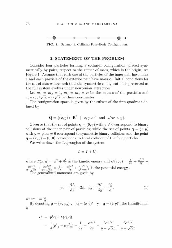
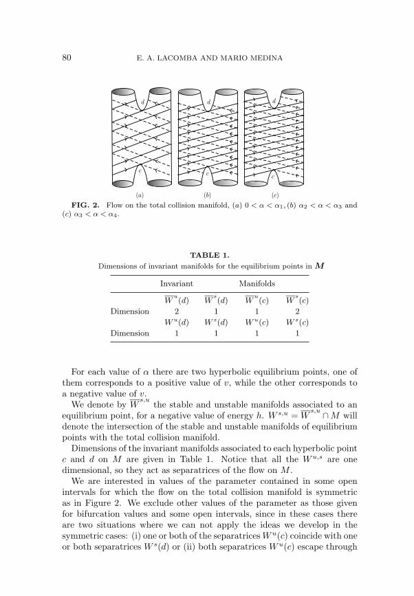
We study a two degrees of freedom problem in celestial mechanics, thecollinear symmetric four body problem, which depends on one positiveparameter given in terms of the masses of the particles. In [5], Lacombaand Simo introduced this problem and obtained valuable information aboutthe nature of the flow on the total collision manifold M , the flow variesaccording the value of the parameter and for values of the parameter insome open intervals the obtained flow on the total collision manifold turnedout to be very symmetric as we can see in Figure 2. The branches of theunstable manifold associated to the equilibrium point c restricted to Mact as separatrices and escape through different upper arms of M aftergiving the same number of turns around it. This feature and the existenceof the homothetic orbit are fundamental for proving the existence of thedesired family of orbits. For values of the parameter outside the consideredintervals the flow may not be symmetric and we can not use the developedmethods to assure the existence of the family of orbits.

75

76 E. A. LACOMBA AND MARIO MEDINA

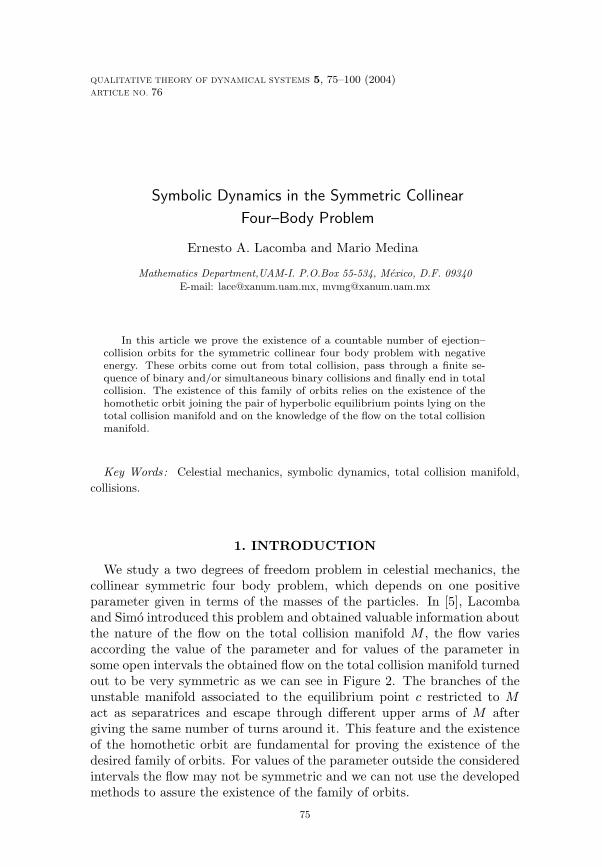
FIG. 1. Symmetric Collinear Four–Body Configuration.

2. STATEMENT OF THE PROBLEM

Consider four particles forming a collinear configuration, placed sym-metrically by pairs, respect to the center of mass, which is the origin, seeFigure 1. Assume that each one of the particles of the inner pair have mass1 and each particle of the exterior pair have mass α. Initial conditions forthe set of masses are such that the symmetric configuration is preserved asthe full system evolves under newtonian attraction.

Let m1 = m2 = 1, m3 = m4 = α be the masses of the particles andx,−x, y/

√α,−y/

√α be their coordinates.

The configuration space is given by the subset of the first quadrant de-fined by

Q = {(x, y) ∈ R2 | x, y > 0 and√

αx < y}.Observe that the set of points q = (0, y) with y 6= 0 correspond to binary

collisions of the inner pair of particles; while the set of points q = (x, y)with y =

√αx 6= 0 correspond to symmetric binary collisions and the point

q = (x, y) = (0, 0) corresponds to total collision of the four particles.We write down the Lagrangian of the system

L = T + U,

where T (x, y) = x2 + y2

α is the kinetic energy and U(x, y) = 12x + α5/2

2y +2α3/2

y−√αx+ 2α3/2

y+√

αx= 1

2x + α5/2

2y + 4α3/2yy2−αx2 is the potential energy .

The generalized momenta are given by

px =∂L

∂x= 2x, py =

∂L

∂y=

2y

α, (1)

where ˙= ddt .

By denoting p = (px py)t, q = (x y)t y q = (x y)t, the Hamiltonianis

H = ptq− L(q, q)

=14(p2

x + αp2y)− 1

2x− α5/2

2y− 2α3/2

y −√αx− 2α3/2

y +√

αx

SYMBOLIC DYNAMICS IN THE SYMMETRIC COLLINEAR 77

=14(p2

x + αp2y)− U(x, y),

and the equations of motion are

q =∂H

∂p, p = −∂H

∂q, (2)

which are written as

x = px

2 , px = − 12x2 + 8α5/2xy

(y2−αx2)2 ,

y = αpy

2 , py = −α5/2

2y2 − 4α3/2 y2+αx2

(y2−αx2)2 .(3)

Next, by using the blow-up technique introduced by McGehee [4], we candescribe the total collision manifold and the flow on this invariant mani-fold. Using this information of the flow on the total collision manifold it ispossible to give a description of the flow near the total collision manifold.

Let I = qtq be the moment of inertia. We define the blow-up of theorigin by the following change of coordinates,

r = I12 , s = r−1q

where r measures the size of the system and s is the configuration or shapeof the system. S = {q ∈ Q | r = 1} is a unit sphere in Q. Coordinates (r,q)represent a polar-like system of coordinates for the configuration space. Itis clear that sts = 1.

If u and v are the (rescaled) tangential and radial components of themomentum given by

u =√

rp− (pts)s, v =√

rpts

with the time reparametrization

dt

dτ= r

32 ,

the equations of motion become

r = rv,

v = utu +v2

2+ U(s),

s = u,

u = −12vu− (utu)s + Grad U(s),


and the energy relation H = h is rewritten as

12(utu + v2) = U(s) + rh.

As we have a two degree of freedom problem, we use canonical polarcoordinates to work with: θ is the usual angular coordinate and the com-ponent of the rescaled velocity in the angular direction, which we shalldenote by u, through the change

s = (cos θ sin θ)t, u = u(cos θ sin θ)t.

In coordinates (r, v, θ, u, τ), the equations of motion are expressed by

r′ = rv,

v′ = u2 +v2

2− U(θ), (4)

θ′ = u,

u′ = −12vu +

dU(θ)dθ

,

where ′ = ddτ . In the same way, the energy relation is transformed into

12(u2 + v2) = U(θ) + rh,

where U(θ) = 12 cos θ + α5/2

2 sin θ + 4α3/2 sin θsin2 θ−α cos2 θ

, θ ∈ (θα, π/2).Our equations still have singularities when the particles of the inner pair

collide or when we have symmetric simultaneous binary collisions, that is,when θ = π/2 or θ = θα, where tan θα =

√α.

In order to simultaneously regularize these singularities, consider thefunction W (θ) = U(θ) cos θ(sin θ −√α cos θ), a new variable

w =cos θ(sin θ −√α cos θ)

2√

W (θ)u,

with the time rescaling

dτ

ds=

cos θ(sin θ −√α cos θ)2√

W (θ).

The equations of motion and the energy relation become


dr

ds= rv

cos θ(sin θ −√α cos θ)2√

W (θ),

dv

ds=

√W (θ)2

{(2rh− 12v2)

cos θ(sin θ −√α cos θ)√W (θ)

+ 1},

dθ

ds= w,

dw

ds= (cos θ(sin θ −√α cos θ)− w2)

dWdθ

2W (θ)− vw cos θ(sin θ −√α cos θ)

2√

2W (θ)

+(cos(2θ) +

√α sin(2θ))

2{3 +

2rh− v2

W (θ)cos θ(sin θ −√α cos θ)}

and

w2 =cos2 θ(sin θ −√α cos θ)2

4W (θ)(2rh− v2) +

cos θ(sin θ −√α cos θ)2

,

respectively. Taking r = 0 in last equation, this can be rewritten as

w2 =cos θ(sin θ −√α cos θ)

2− v2 cos2 θ(sin θ −√α cos θ)2

4W (θ). (5)

In this way we have extended the vector field to the components deter-mined by binary and simultaneous binary collisions. We define the totalcollision manifold as the set

M = {(r, v, θ, w) | r = 0, equation (5) holds, and θα ≤ θ ≤ π/2}.

3. DESCRIPTION OF THE FLOW ON THE TOTALCOLLISION MANIFOLD

Next we give some features of the flow on the total collision manifoldobtained by using the blow up technique.

For a value of the parameter α, the equilibrium points are (r = 0, v =

±√

U(θα), θ = θα, w = 0), which lie on the total collision manifold M .All equilibrium points are hyperbolic. Also, the flow on the total collisionmanifold is almost gradient with respect to v. In Figure 2 we show the flowon the total collision manifold for different values of α as obtained in [5].


d

cc

c

d d

( )a ( )b ( )c

FIG. 2. Flow on the total collision manifold, (a) 0 < α < α1, (b) α2 < α < α3 and(c) α3 < α < α4.

TABLE 1.

Dimensions of invariant manifolds for the equilibrium points in M

Invariant Manifolds

Wu(d) W

s(d) W

u(c) W

s(c)

Dimension 2 1 1 2

W u(d) W s(d) W u(c) W s(c)

Dimension 1 1 1 1

For each value of α there are two hyperbolic equilibrium points, one ofthem corresponds to a positive value of v, while the other corresponds toa negative value of v.

We denote by Ws,u

the stable and unstable manifolds associated to anequilibrium point, for a negative value of energy h. W s,u = W

s,u ∩M willdenote the intersection of the stable and unstable manifolds of equilibriumpoints with the total collision manifold.

Dimensions of the invariant manifolds associated to each hyperbolic pointc and d on M are given in Table 1. Notice that all the Wu,s are onedimensional, so they act as separatrices of the flow on M .

We are interested in values of the parameter contained in some openintervals for which the flow on the total collision manifold is symmetricas in Figure 2. We exclude other values of the parameter as those givenfor bifurcation values and some open intervals, since in these cases thereare two situations where we can not apply the ideas we develop in thesymmetric cases: (i) one or both of the separatrices Wu(c) coincide with oneor both separatrices W s(d) or (ii) both separatrices Wu(c) escape through


the same upper arm of M . In [5] page 61, the authors obtained severalbifurcation values for α, (αk, αi < αi+1), and in consequence, intervalsdefined by these parameter values. The intervals we are interested in areintervals like (0, α1), (α2, α3) and (α3, α4). For values in these intervals thecorresponding flow is as given in Figure 2, rather symmetric.

4. EXISTENCE OF THE HOMOTHETIC ORBIT

For negative values of the energy h we shall prove the existence of ahomothetic orbit contained in W

s(c) ∩ W

u(d), located outside the total

collision manifold and joining the equilibrium points c and d. This ho-mothetic orbit will be of great importance in order to give the desireddescription of the family of orbits which come out from total collision, passthrough a sequence of binary collisions of the particles of the inner pairand/or simultaneous binary collisions, and finally end in total collision.

Recall that homothetic solutions are characterized by the fact that θ ≡θα, where U ′(θα) = 0. By using system (4) of equations, we can obtaina parametric representation of the homothetic orbit. When θ ≡ θα, thenu = 0 and, in consequence we have equations

dr

dτ= rv,

dv

dτ=

v2

2− U(θα),

so,

dv

2U(θα)− v2=

dτ

−2,

taking vα =√

2U(θα), we get

tanh−1(v

vα) = −τvα

2,

that is

v(τ) = −vα tanh(τvα/2).

Using the expression for v(τ), we obtain

r(τ) = − U(θα)h cosh2(τvα/2)

.

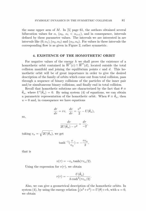
Also, we can give a geometrical description of the homothetic orbits. Insystem (4), by using the energy relation 1

2 (u2+v2) = U(θ)+rh, with u = 0,we obtain


r

v

h<0

h=0

h=0

FIG. 3. Homothetic orbits in the plane u = 0, θ = θα.

dr

dτ= rv,

dv

dτ= rh.

By solving this system of differential equations, we get

v2 = 2rh + m.

These solutions can be seen as restrictions of the energy relation to theplane u = 0, θ = θα; that is v2

2 = rh + U(θα), so we have m = 2U(θα).For each negative value of h, we have an orbit coming out from one of theequilibrium points and ending at the other equilibrium point, as seen inFigure 3.

Definition 1. We say that an orbit having c as ω-limit is an orbitwhich ends in total collision or a total collision orbit and an orbit havingd as α-limit is an ejection orbit or an orbit coming out from total collision.

In this way, all orbits contained in Wu(d) are ejection orbits and those

contained in Ws(c) are total collision orbits. Orbits contained in W

s(c) ∩

Wu(d) will be called ejection-collision orbits.

5. POINCARE-SECTION AND BASIC RESULTS

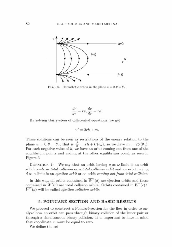
We proceed to construct a Poincare-section for the flow in order to an-alyze how an orbit can pass through binary collision of the inner pair orthrough a simultaneous binary collision. It is important to have in mindthat coordinate w must be equal to zero.

We define the set


ΓL

v

r

ΓR

r

v

l

l

FIG. 4. Section of binary and simultaneous binary collisions

Γ = {(r, v, θ, w) | r ≥ 0, θ = θα, π/2, w = 0},which is the union of two half-planes,

ΓL = {(r, v, θ, w) | r ≥ 0, θ = θα, w = 0},

and

ΓR = {(r, v, θ, w) | r ≥ 0, θ = π/2, w = 0},that are parametrized by coordinates (r, v) ∈ [0,∞)×R. See Figure 4.

Observe that lines l1 and l2 in Figure 4 correspond to lines r = 0 con-tained in the half-planes ΓL and ΓR, respectively.

Now, we obtain the first intersection in positive time of Wu(d) with Γ

following ideas contained in [2] and [3].

Proposition 2. The first intersection in positive time of Wu(d) and

Γ contains two arcs σR,L, contained in ΓR,L and with extremes on theboundaries of ΓR,L (lines l1 and l2 respectively).

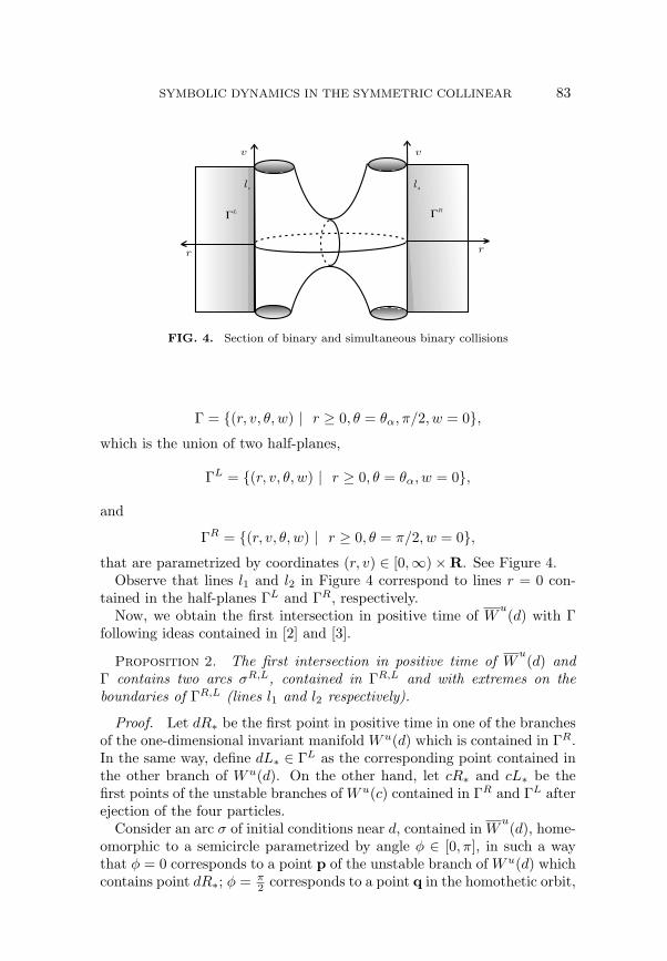
Proof. Let dR∗ be the first point in positive time in one of the branchesof the one-dimensional invariant manifold Wu(d) which is contained in ΓR.In the same way, define dL∗ ∈ ΓL as the corresponding point contained inthe other branch of Wu(d). On the other hand, let cR∗ and cL∗ be thefirst points of the unstable branches of Wu(c) contained in ΓR and ΓL afterejection of the four particles.

Consider an arc σ of initial conditions near d, contained in Wu(d), home-

omorphic to a semicircle parametrized by angle φ ∈ [0, π], in such a waythat φ = 0 corresponds to a point p of the unstable branch of Wu(d) whichcontains point dR∗; φ = π

2 corresponds to a point q in the homothetic orbit,


c

σR

dR*

cR*

q

pd

FIG. 5. First intersection in positive time of Wu(d) with ΓR.

and φ = π corresponds to a point t in the branch of the unstable branchof Wu(d) containing dL∗.

In order to find the first intersection point of Wu(d), in positive time,

with Γ, we follow the semicircle σ of initial conditions under the flow. First,we consider the segment of the semicircle parametrized by φ ∈ [0, π/2], so,point p goes, under the flow, to point dR∗ ∈ ΓR and points in this subarc,near p go to points in ΓR, near dR∗; on the other hand, points near q gonear c and, then, continuing near the unstable branch of c, pass close tocR∗. The subarc of σ, parametrized by [0, π/2], being a continuous arc, itsimage under the flow must be a continuous arc which we denote by σR, andis contained in ΓR. Its extremes are denoted by dR∗ and cR∗, as shown inFigure 5. In an analogous way, the image of the subarc parametrized by[π/2, π] is also a continuous arc σL, contained in ΓL, with extremes dL∗and cL∗ in line {r = 0} ∩ ΓL.

Let R∗d and L∗d be those points on the stable branches of W s(d), con-tained in ΓR and ΓL that go to d, but such that no other point in theirpositive time orbits are contained in ΓR or ΓL. In the same way we definepoints R∗c ∈ ΓR and L∗c ∈ ΓL as those points in W s(c), so that theirpositive time orbits do not intersect ΓR nor ΓL.

Proposition 3. The last intersection, in positive time of Ws(c) with Γ

is given by two arcs γR,L, contained in ΓR,L, whose extremes (of the arcs)given by R∗d, R∗c and L∗d, L∗c are contained on the boundary of ΓR,L

(lines l1 and l2, respectively).

Proof. Using the symmetry given by the reversibility of the originalHamiltonian system for the symmetric collinear four body problem and


γR

=R C*

σR

=ER*

R d*

cR*

dR*

R c*

γ1

R

γ2

R

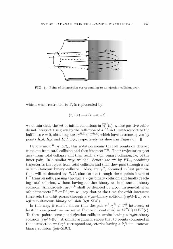
FIG. 6. Point of intersection corresponding to an ejection-collision orbit.

which, when restricted to Γ, is represented by

(r, v, t) −→ (r,−v,−t),

we obtain that, the set of initial conditions in Ws(c), whose positive orbits

do not intersect Γ is given by the reflection of σR,L in Γ, with respect to thehalf lines v = 0, obtaining arcs γR,L ⊂ ΓR,L, which have extremes given bypoints R∗d, R∗c and L∗d, L∗c, respectively, as shown in Figure 6.

Denote arc σR by ER∗, this notation means that all points on this arccome out from total collision and then intersect ΓR. Their trajectories ejectaway from total collapse and then reach a right binary collision, i.e. of theinner pair. In a similar way, we shall denote arc σL by EL∗, obtainingtrajectories that eject from total collision and then they pass through a leftor simultaneous binary collision. Also, arc γR, obtained in last proposi-tion, will be denoted by R∗C, since orbits through these points intersectΓR transversally, passing through a right binary collision and finally reach-ing total collision, without having another binary or simultaneous binarycollision. Analogously, arc γL shall be denoted by L∗C. In general, if anorbit intersects ΓR or ΓL, we will say that at the time the orbit intersectsthese sets the orbit passes through a right–binary collision (right–BC) or aleft–simultaneous binary collision (left–SBC).

In this way, it can be shown that the pair σR, γR ⊂ ΓR intersect, atleast in one point, as we see in Figure 6, contained in W

u(d) ∩ W

s(c).

To these points correspond ejection-collision orbits having a right binarycollision (right–BC). A similar argument shows that to points contained inthe intersection σL ∩ γL correspond trajectories having a left simultaneousbinary collision (left–SBC).


To each one of these ejection-collision orbits having a right–BC (left–SBC) we associate a sequence of symbols of the form ERC (ELC), whichmeans that these orbits eject from total collision, pass through a right–BC(left–SBC) and then go directly to total collision without having anotherbinary or simultaneous binary collision.

Next, we characterize the pullbacks of Ws(c)∩Γ under the Poincare map

P : Γ −→ Γ

also known as the first return map which is defined as follows. Let p a pointin Γ so that its positive orbit φ(t, p) intersects Γ transversally at time Tand φ(t, p), for t ∈ (0, T ), does not intersect Γ; for points in Γ near p theirtrajectories return to Γ in time close to T . The map associates to points xin Γ near p their points of first return to Γ. To be more precise, for x in Γclose to p

P (x) = φ(τ(x), x)

where τ(x) is the time of first return of the orbit through point x to Γ.The following results will be of fundamental importance for characteriz-

ing all orbits passing through binary or simultaneous binary collisions.

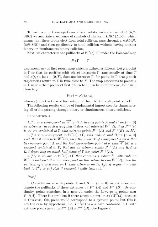
Proposition 4.

1.If σ is a subsegment in Ws(c) ∩ Γ, having points A and B on {r = 0}

as extremes, in such a way that it does not intersect Wu(d), then P−1(σ)

is an arc contained in Γ with extreme points P−1(A) and P−1(B) on M .2.If σ is a subsegment in W

s(c) ∩ Γ, with ends A and B on {r = 0}

such that it intersects Wu(d), then the pullback of subsegment σ on σ that

lies between point A and the first intersection point of σ with Wu(d) is a

segment contained in Γ, that has as extreme points P−1(A) and R∗d orL∗d depending on which half-plane of Γ lies point P−1(A).

3.If γ is an arc in Ws(c) ∩ Γ that contains a subarc γ, with ends on

Wu(d) and such that no other point on this subarc lies on W

u(d), then the

pullback of γ is a loop on Γ with extremes on (i) L∗d if segment γ pullsback to ΓR, or (ii) R∗d if segment γ pulls back to ΓL.

Proof.

1. Consider arc σ with points A and B on {r = 0} as extremes, anddenote the pullbacks of these extremes by P−1(A) and P−1(B). By con-tinuity, points contained in σ near A, under the flow, go to points nearP−1(A). There is a problem if there exists a point on σ ∩W

u(d), because

in this case, this point would correspond to a ejection point, but this isnot the case by hypothesis. So, P−1(σ) is a subarc contained in Γ withextreme points given by P−1(A) y P−1(B). See Figure 7.


*P A

1

( )

P B1

( )

P1

( )σ

FIG. 7. Pullback of an arc segment in Proposition 4, case 1.

r=0

R d*

γ~

~

Wu

( )d

P1

( γ )

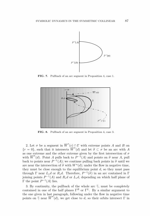
FIG. 8. Pullback of an arc segment in Proposition 4, case 3.

2. Let σ be a segment in Ws(c) ∩ Γ with extreme points A and B on

{r = 0}, such that it intersects Wu(d) and let σ ⊂ σ be an arc with A

as one extreme and the other extreme given by the first intersection of σwith W

u(d). Point A pulls back to P−1(A) and points on σ near A, pull

back to points near P−1(A); we continue pulling back points in σ until weare near the intersection of σ with Wu(d); under the flow in negative time,they must be close enough to the equilibrium point d, so they must passthrough Γ near L∗d or R∗d. Therefore, P−1(σ) in an arc contained in Γjoining points P−1(A) and R∗d or L∗d, depending on which half plane ofΓ the point P−1(A) lies.

3. By continuity, the pullback of the whole arc γ, must be completelycontained in one of the half planes ΓR or ΓL. By a similar argument tothe one given in last paragraph, following under the flow in negative timepoints on γ near W

u(d), we get close to d, so their orbits intersect Γ in


dR*

ER*

R d*

R c*

cR*

dL*

L d*

cL*

L c*

EL*

R1

R

R

R

R

R

R

R

R

R

γ1

Rγ

1

L

( )γ1

R

P2

( )γ1

R

P1

( )γ1

L

P2

( )γ1

L

P1

FIG. 9. Pullback of an arc segment in Corollary 5, case (2).

points near the stable branches of d contained in M ; that is, must passclose to R∗d or L∗d. But the pullback of γ is entirely contained in thesame half plane, so the pullback is a loop with extremes in R∗d or L∗d aswe can see in Figure 8.

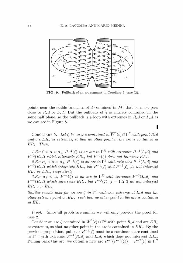
Corollary 5. Let ζ be an arc contained in Ws(c)∩ΓR with point R∗d

and arc ER∗ as extremes, so that no other point in the arc is contained inER∗. Then,

1.For 0 < α < α1, P−2(ζ) is an arc in ΓR with extremes P−1(L∗d) andP−2(R∗d) which intersects ER∗, but P−1(ζ) does not intersect EL∗.

2.For α2 < α < α3, P−3(ζ) is an arc in ΓL with extremes P−2(L∗d) andP−3(R∗d) which intersects EL∗, but P−1(ζ) and P−2(ζ) do not intersectEL∗ or ER∗, respectively.

3.For α3 < α, P−4(ζ) is an arc in ΓR with extremes P−3(L∗d) andP−4(R∗d) which intersects ER∗, but P−j(ζ), j = 1, 2, 3 do not intersectER∗ nor EL∗.

Similar results hold for an arc ζ in ΓL with one extreme at L∗d and theother extreme point on EL∗, such that no other point in the arc is containedin EL∗

Proof. Since all proofs are similar we will only provide the proof forcase 2.

Consider an arc ζ contained in Ws(c)∩ΓR with point R∗d and arc ER∗

as extremes, so that no other point in the arc is contained in ER∗. By theprevious proposition, pullback P−1(ζ) must be a continuous arc containedin ΓL, with extremes P−1(R∗d) and L∗d, which does not intersect EL∗.Pulling back this arc, we obtain a new arc P−1(P−1(ζ)) = P−2(ζ) in ΓR


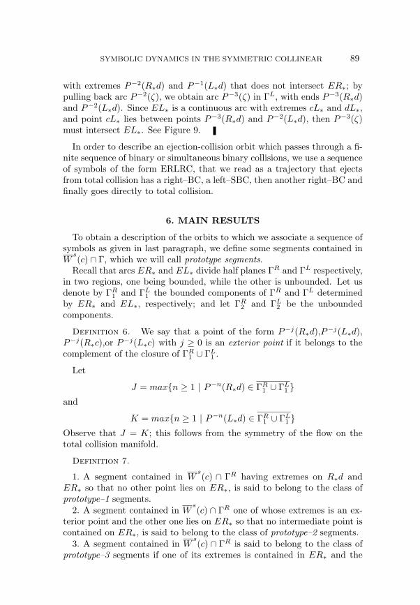
with extremes P−2(R∗d) and P−1(L∗d) that does not intersect ER∗; bypulling back arc P−2(ζ), we obtain arc P−3(ζ) in ΓL, with ends P−3(R∗d)and P−2(L∗d). Since EL∗ is a continuous arc with extremes cL∗ and dL∗,and point cL∗ lies between points P−3(R∗d) and P−2(L∗d), then P−3(ζ)must intersect EL∗. See Figure 9.

In order to describe an ejection-collision orbit which passes through a fi-nite sequence of binary or simultaneous binary collisions, we use a sequenceof symbols of the form ERLRC, that we read as a trajectory that ejectsfrom total collision has a right–BC, a left–SBC, then another right–BC andfinally goes directly to total collision.

6. MAIN RESULTS

To obtain a description of the orbits to which we associate a sequence ofsymbols as given in last paragraph, we define some segments contained inW

s(c) ∩ Γ, which we will call prototype segments.

Recall that arcs ER∗ and EL∗ divide half planes ΓR and ΓL respectively,in two regions, one being bounded, while the other is unbounded. Let usdenote by ΓR

1 and ΓL1 the bounded components of ΓR and ΓL determined

by ER∗ and EL∗, respectively; and let ΓR2 and ΓL

2 be the unboundedcomponents.

Definition 6. We say that a point of the form P−j(R∗d),P−j(L∗d),P−j(R∗c),or P−j(L∗c) with j ≥ 0 is an exterior point if it belongs to thecomplement of the closure of ΓR

1 ∪ ΓL1 .

Let

J = max{n ≥ 1 | P−n(R∗d) ∈ ΓR1 ∪ ΓL

1 }and

K = max{n ≥ 1 | P−n(L∗d) ∈ ΓR1 ∪ ΓL

1 }Observe that J = K; this follows from the symmetry of the flow on thetotal collision manifold.

Definition 7.

1. A segment contained in Ws(c) ∩ ΓR having extremes on R∗d and

ER∗ so that no other point lies on ER∗, is said to belong to the class ofprototype–1 segments.

2. A segment contained in Ws(c) ∩ ΓR one of whose extremes is an ex-

terior point and the other one lies on ER∗ so that no intermediate point iscontained on ER∗, is said to belong to the class of prototype–2 segments.

3. A segment contained in Ws(c) ∩ ΓR is said to belong to the class of

prototype–3 segments if one of its extremes is contained in ER∗ and the


other is given by P−J (R∗d) or P−J(L∗d), depending on which of them iscontained in the bounded component in ΓR determined by ER∗.

4. A segment in Ws(c) ∩ ΓL is called to belong to the the class of

prototype–4 segments if one of the extremes is L∗d and the other extremelies on EL∗, so that no other point of the segment is contained on EL∗.

5. A segment contained in Ws(c) ∩ ΓL so that one of its extremes is an

exterior point and the other extreme lies on EL∗ so that no other point ofthe segment is contained on EL∗, is said to belong to the class of prototype–5 segments.

6. A segment contained in Ws(c) ∩ ΓL is said to belong to the class of

prototype–6 segments if one of its extremes is contained in EL∗ and theother one is given by P−J (R∗d) or P−J(L∗d), depending on which of themis contained in the bounded component in ΓL determined by EL∗.

Remark 8. A segment belonging to the class of prototype-i segmentswill be said to belong to Prot(i) and will be denoted by Prot(i). SegmentsProt(2) and Prot(5) are contained in the unbounded components, whileall the others are contained in the bounded ones.

By using Proposition 3 and its Corollary 1 we obtain the existence of aninfinite number of segments contained in W

s(c) ∩ ΓR,L and belonging to

each one of the above defined six classes of prototype-i segments. Observethat segments belonging to the three first classes are subsets of ΓR andthose belonging to the other three classes are subsets of ΓL. All of thisreflects the geometric symmetries of the symmetric collinear four bodyproblem and the symmetry due to the reversibility of the problem.

Now, we show some examples of segments contained in Ws(c) and be-

longing to each one of the classes of prototype segments.

Example 9. For examples in classes Prot(i), i = 1, 2 we refer to Figures6 and 12. Segment γR

1 contained in γR, having one extreme at R∗d andthe other extreme on ER∗, so that no other point is contained in ER∗ is asegment in the class of prototype–1 segments. Segment γR

2 contained in γR,with one extreme at R∗c and the other extreme on ER∗ so that no otherpoint in γR

2 is contained in ER∗ is a segment in the class of prototype–2segments. In order to obtain an example of a prototype–3 segment considerP−(J+1)(γR

1 ); we know by Corollary 1 that this arc intersects ER∗, theexample we are looking for is defined by the subsegment of P−(J+1)(γR

1 )with one end given by P−J (R∗d) or P−J (L∗d) depending on which ofthese points lies on the bounded component determined by ER∗ while theother end is the first intersection of P−(J+1)(γR

1 ) with ER∗ and no otherpoint in the considered segment is contained in ER∗. For a graphicalrepresentation in case α2 < α < α3, see Figure 9, and replace segment ζby segment γR

1 already defined. Next, examples for Prot(i),i = 4, 5, 6 are


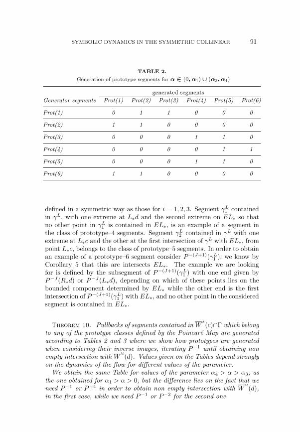
TABLE 2.

Generation of prototype segments for α ∈ (0, α1) ∪ (α3, α4)

generated segments

Generator segments Prot(1) Prot(2) Prot(3) Prot(4) Prot(5) Prot(6)

Prot(1) 0 1 1 0 0 0

Prot(2) 1 1 0 0 0 0

Prot(3) 0 0 0 1 1 0

Prot(4) 0 0 0 0 1 1

Prot(5) 0 0 0 1 1 0

Prot(6) 1 1 0 0 0 0

defined in a symmetric way as those for i = 1, 2, 3. Segment γL1 contained

in γL, with one extreme at L∗d and the second extreme on EL∗ so thatno other point in γL

1 is contained in EL∗, is an example of a segment inthe class of prototype–4 segments. Segment γL

2 contained in γL with oneextreme at L∗c and the other at the first intersection of γL with EL∗, frompoint L∗c, belongs to the class of prototype–5 segments. In order to obtainan example of a prototype–6 segment consider P−(J+1)(γL

1 ), we know byCorollary 5 that this arc intersects EL∗. The example we are lookingfor is defined by the subsegment of P−(J+1)(γL

1 ) with one end given byP−J(R∗d) or P−J (L∗d), depending on which of these points lies on thebounded component determined by EL∗ while the other end is the firstintersection of P−(J+1)(γL

1 ) with EL∗, and no other point in the consideredsegment is contained in EL∗.

Theorem 10. Pullbacks of segments contained in Ws(c)∩Γ which belong

to any of the prototype classes defined by the Poincare Map are generatedaccording to Tables 2 and 3 where we show how prototypes are generatedwhen considering their inverse images, iterating P−1 until obtaining nonempty intersection with W

u(d). Values given on the Tables depend strongly

on the dynamics of the flow for different values of the parameter.We obtain the same Table for values of the parameter α4 > α > α3, as

the one obtained for α1 > α > 0, but the difference lies on the fact that weneed P−1 or P−4 in order to obtain non empty intersection with W

u(d),

in the first case, while we need P−1 or P−2 for the second one.


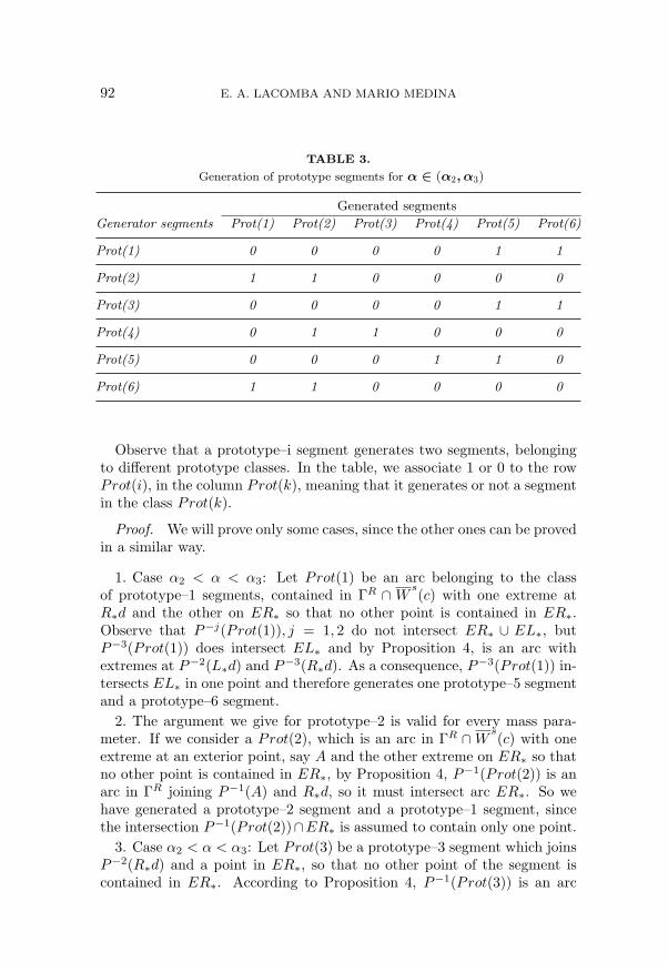
TABLE 3.

Generation of prototype segments for α ∈ (α2, α3)

Generated segments

Generator segments Prot(1) Prot(2) Prot(3) Prot(4) Prot(5) Prot(6)

Prot(1) 0 0 0 0 1 1

Prot(2) 1 1 0 0 0 0

Prot(3) 0 0 0 0 1 1

Prot(4) 0 1 1 0 0 0

Prot(5) 0 0 0 1 1 0

Prot(6) 1 1 0 0 0 0

Observe that a prototype–i segment generates two segments, belongingto different prototype classes. In the table, we associate 1 or 0 to the rowProt(i), in the column Prot(k), meaning that it generates or not a segmentin the class Prot(k).

Proof. We will prove only some cases, since the other ones can be provedin a similar way.

1. Case α2 < α < α3: Let Prot(1) be an arc belonging to the classof prototype–1 segments, contained in ΓR ∩ W

s(c) with one extreme at

R∗d and the other on ER∗ so that no other point is contained in ER∗.Observe that P−j(Prot(1)), j = 1, 2 do not intersect ER∗ ∪ EL∗, butP−3(Prot(1)) does intersect EL∗ and by Proposition 4, is an arc withextremes at P−2(L∗d) and P−3(R∗d). As a consequence, P−3(Prot(1)) in-tersects EL∗ in one point and therefore generates one prototype–5 segmentand a prototype–6 segment.

2. The argument we give for prototype–2 is valid for every mass para-meter. If we consider a Prot(2), which is an arc in ΓR ∩W

s(c) with one

extreme at an exterior point, say A and the other extreme on ER∗ so thatno other point is contained in ER∗, by Proposition 4, P−1(Prot(2)) is anarc in ΓR joining P−1(A) and R∗d, so it must intersect arc ER∗. So wehave generated a prototype–2 segment and a prototype–1 segment, sincethe intersection P−1(Prot(2))∩ER∗ is assumed to contain only one point.

3. Case α2 < α < α3: Let Prot(3) be a prototype–3 segment which joinsP−2(R∗d) and a point in ER∗, so that no other point of the segment iscontained in ER∗. According to Proposition 4, P−1(Prot(3)) is an arc


ER*

P Prot k--j

( ( ))

r=0

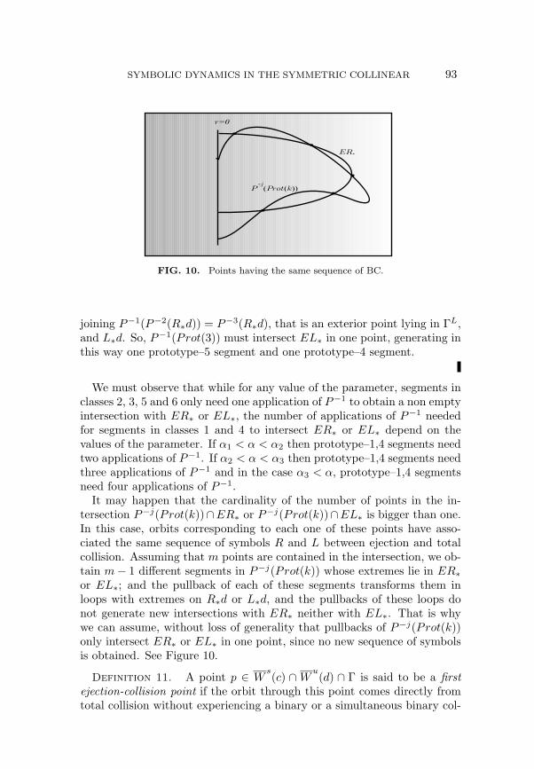
FIG. 10. Points having the same sequence of BC.

joining P−1(P−2(R∗d)) = P−3(R∗d), that is an exterior point lying in ΓL,and L∗d. So, P−1(Prot(3)) must intersect EL∗ in one point, generating inthis way one prototype–5 segment and one prototype–4 segment.

We must observe that while for any value of the parameter, segments inclasses 2, 3, 5 and 6 only need one application of P−1 to obtain a non emptyintersection with ER∗ or EL∗, the number of applications of P−1 neededfor segments in classes 1 and 4 to intersect ER∗ or EL∗ depend on thevalues of the parameter. If α1 < α < α2 then prototype–1,4 segments needtwo applications of P−1. If α2 < α < α3 then prototype–1,4 segments needthree applications of P−1 and in the case α3 < α, prototype–1,4 segmentsneed four applications of P−1.

It may happen that the cardinality of the number of points in the in-tersection P−j(Prot(k))∩ER∗ or P−j(Prot(k))∩EL∗ is bigger than one.In this case, orbits corresponding to each one of these points have asso-ciated the same sequence of symbols R and L between ejection and totalcollision. Assuming that m points are contained in the intersection, we ob-tain m− 1 different segments in P−j(Prot(k)) whose extremes lie in ER∗or EL∗; and the pullback of each of these segments transforms them inloops with extremes on R∗d or L∗d, and the pullbacks of these loops donot generate new intersections with ER∗ neither with EL∗. That is whywe can assume, without loss of generality that pullbacks of P−j(Prot(k))only intersect ER∗ or EL∗ in one point, since no new sequence of symbolsis obtained. See Figure 10.

Definition 11. A point p ∈ Ws(c) ∩ W

u(d) ∩ Γ is said to be a first

ejection-collision point if the orbit through this point comes directly fromtotal collision without experiencing a binary or a simultaneous binary col-


lision in between. In the same way, a point p ∈ Ws(c)∩W

u(d)∩Γ is called

a last ejection-collision point if the orbit through this point goes directlyto total collision without experiencing a binary or a simultaneous binarycollision in between.

Next, we show how to use Tables 2 and 3 given in Theorem 10 to generatea family of ejection–collision orbits that have a finite sequence of binary orsimultaneous binary collisions. In order to do this, we begin by analyzingthe pullbacks of prototype segments contained in γR and γL. We describenow families of ejection-collision orbits that show distinct dynamics.

The following result shows the existence of a family of ejection–collisionorbits having n–binary collisions or n–simultaneous binary collisions forn ≥ 1. It is clear that they are different from the homothetic orbit, whichis free from collisions.

Proposition 12. For any value of the parameter α, for each n ≥ 1,there exist a type ERnC orbit, and a type ELnC orbit.

Proof. We will prove the existence of the family of orbits having relatedsequences given by ERnC, since the existence of the other family is provedin a symmetric way.

We know that points contained in γR ∩ σR are first and last ejection–collision points, so their orbits have associated sequences of the form ERC.When considering subsegment γR

2 of γR, its pullback P−1(γR2 ) intersects

ER∗, and generates two segments, one of prototype–1, and one of prototype–2; through the point of intersection of P−1(γR

2 ) with ER∗ (remember weare assuming there is only one intersection point) passes an orbit with as-sociated sequence ERRC. According to Theorem 10, the new prototype–2segment, under P−1 intersects ER∗ and generates another prototype–1segment and a prototype–2 segment, and to the common point of thesetwo resulting segments corresponds an orbit with a sequence of the formERRRC. Continuing this process of iterating all prototype–2 segmentsobtained at each step, it is possible to construct the desired family of or-bits.

Proposition 13. For 0 < α < α1, there are ejection-collision orbitswhich perform a sequence of n (n ≥ 1) binary and/or simultaneous binarycollisions.

Proof. As we know, arcs γR and σR in ΓR, contained in Ws(c) and

Wu(d), respectively, intersect, generating two segments, one prototype–1

segment and one prototype–2 segment: γR1 and γR

2 , which are subsegmentsof γR and their common point, which is unique by assumption, is a first andlast ejection-collision point. By Theorem 10, by iterating these two proto-type segments under P−1, we obtain according to Table 2, four prototypesegments : say, one Prot(2) and one Prot(3) for γR

1 and, one Prot(1) and


Prot(2) for γR2 and two first and last ejection-collision points, given by the

common point of each one of the pairs of the given prototype segments, astwo ejection-collision orbits having three and two binary and simultaneousbinary collisions, respectively. This way, we can continue this process ofiteration of P−1 for each one of the obtained four prototype segments. Thisis possible due to Theorem 10. Each of the four segments need to be iter-ated, under P−1, once or twice in order to obtain a non empty intersectionwith ER∗ or EL∗.

So, we can assume that we have an orbit with associated sequence givenby EQ1Q2 . . . QnC, where Qi ∈ {R, L}; moreover, the last symbol Qn

before total collision was obtained through two prototype segments, sayProt(k) and Prot(j). Iterating one of these two prototype segments wecan obtain a new trajectory having one or two last new symbols Qn+1,or Qn+1Qn+2. This depends on whether we require one or two iterationsunder P−1 of the given prototype segments, in order to obtain a non emptyintersection with ER∗ or EL∗. Then we have obtained an orbit with asso-ciated sequence of symbols given by

EQ1Q2 . . . QnQn+1C or EQ1Q2 . . . QnQn+1Qn+2C.

Corollary 14. For 0 < α < α1, there are ejection-collision orbitsof the type ERLRC. By symmetry, orbits of the type are ELRLC areobtained .

Proof. Consider the segment γR1 contained in γR. By Theorem 10,

its pullback P−1(γR1 ), does not intersect ER∗ nor EL∗, but P−2(γR

1 ) doesintersect ER∗, obtaining a prototype–2 and a prototype–3 segment, and thecommon point is a first ejection-collision point. Iterating this point underP , we have that the first iteration is a point in ΓL and the second one isa point in ΓR, which is a last ejection-collision point. So, to these threepoints corresponds an orbit with associated sequence given by ERLRC.

Corollary 15. The following statements hold.

1.For α2 < α < α3, there are ejection-collision trajectories with ELRLRC as associated sequence, and by symmetry, trajectories with sequencesERLRLC are obtained.

2.For α3 < α, there are ejection-collision trajectories with associated se-quences ERLRLRC, and by symmetry, trajectories with sequences ELRLRLC are obtained.


Proof.

1. Consider segment γR1 ; contained in γR, according to Table 2, the

pullbacks P−1(γR1 ), and P−2(γR

1 ) do not intersect neither ER∗ nor EL∗,but P−3(γR

1 ) does intersect EL∗, obtaining a prototype–5 and a prototype–6 segment and a first ejection–collision point p. Iterating this first ejection–collision point under P we obtain that its first iteration give us a point inΓR; the second iteration of the point lies in ΓL and the third iteration givesus a last ejection–collision point contained in ΓR. So, we can associate asequence of the form ELRLRC to point p. The existence of the other orbitwith associated sequence ERLRLC is obtained by symmetry.

2. The proof of this part is completely similar to the above one.

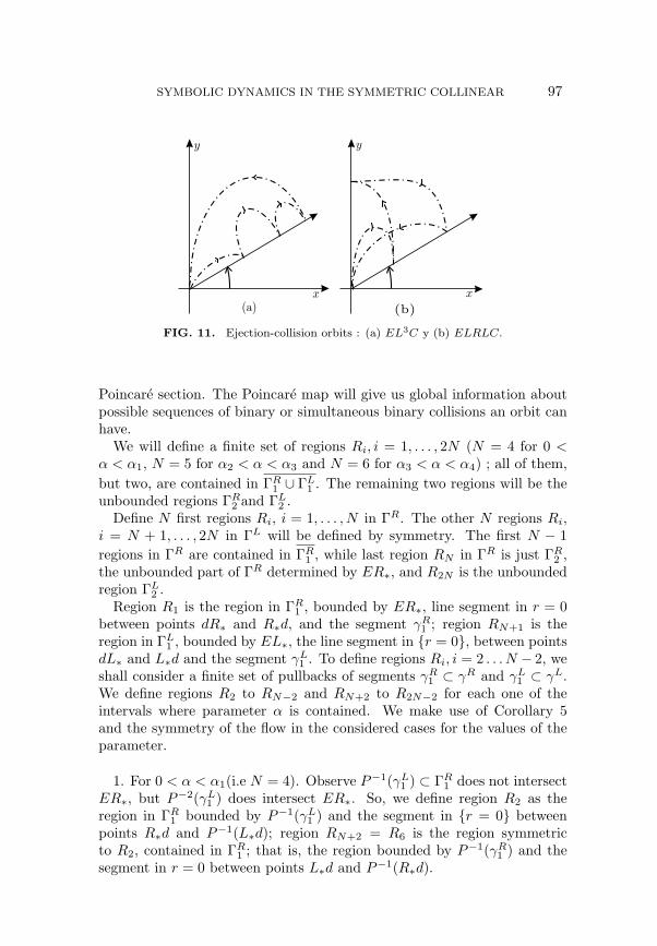
In order to end this section, we give an interpretation to sequences ofsymbols of the form EQ1Q2 . . . Qj . . . QmC, with Qj ∈ {R, L}, which areassociated to ejection-collision trajectories having a finite set of binary orsimultaneous binary collision in terms of the original coordinates x, y forthe symmetric collinear four body problem.

Recall that binary and simultaneous binary collisions correspond to x =0, y 6= 0 and y =

√αx 6= 0, respectively. Under the McGehee transfor-

mation these singularities correspond to values of θ given by θ = π/2 andθ = θα, respectively. So, when in McGehee coordinates θ = π/2, we have abinary collision of the inner pair of the collinear configuration, while havingθ = θα means that we have a simultaneous binary collision. Observe thatwe did not consider the case x = y = 0, because in this case total collisionoccurs.

Taking into account this information, and the fact that to symbol Lcorresponds a point in ΓL, then an orbit where a symbol Qj = L appearsin its associated sequence EQ1Q2 . . . Qj . . . QmC, performs a simultaneousbinary collision when crossing ΓL. In the case symbol Qj = R appears inthe sequence, then a binary collision of the inner pair occurs at the timethe orbit crosses ΓR.

In this way, sequences ERnC and ELnC obtained in Proposition 12 forany value of α, are associated to ejection-collision orbits that either havea sequence of n simultaneous binary collisions or a sequence of n binarycollisions of the inner pair, respectively. A similar interpretation of thesequences ERLRC and ELRLC obtained in Corollary 14, can be given,as we see in Figure 11.

Next, we give a description of orbits, not necessarily ejection-collisionorbits which pass through a sequence of binary or simultaneous binary col-lisions. In order to do this, we shall study iterations, under the inverse P−1

of the Poincare Map of regions, instead of segments, as done in [3] and [1].The regions are contained in Γ = ΓR ∪ ΓL, which has been our convenient


x

y y

x

(a) (b)

FIG. 11. Ejection-collision orbits : (a) EL3C y (b) ELRLC.

Poincare section. The Poincare map will give us global information aboutpossible sequences of binary or simultaneous binary collisions an orbit canhave.

We will define a finite set of regions Ri, i = 1, . . . , 2N (N = 4 for 0 <α < α1, N = 5 for α2 < α < α3 and N = 6 for α3 < α < α4) ; all of them,but two, are contained in ΓR

1 ∪ ΓL1 . The remaining two regions will be the

unbounded regions ΓR2 and ΓL

2 .Define N first regions Ri, i = 1, . . . , N in ΓR. The other N regions Ri,

i = N + 1, . . . , 2N in ΓL will be defined by symmetry. The first N − 1regions in ΓR are contained in ΓR

1 , while last region RN in ΓR is just ΓR2 ,

the unbounded part of ΓR determined by ER∗, and R2N is the unboundedregion ΓL

2 .Region R1 is the region in ΓR

1 , bounded by ER∗, line segment in r = 0between points dR∗ and R∗d, and the segment γR

1 ; region RN+1 is theregion in ΓL

1 , bounded by EL∗, the line segment in {r = 0}, between pointsdL∗ and L∗d and the segment γL

1 . To define regions Ri, i = 2 . . . N − 2, weshall consider a finite set of pullbacks of segments γR

1 ⊂ γR and γL1 ⊂ γL.

We define regions R2 to RN−2 and RN+2 to R2N−2 for each one of theintervals where parameter α is contained. We make use of Corollary 5and the symmetry of the flow in the considered cases for the values of theparameter.

1. For 0 < α < α1(i.e N = 4). Observe P−1(γL1 ) ⊂ ΓR

1 does not intersectER∗, but P−2(γL

1 ) does intersect ER∗. So, we define region R2 as theregion in ΓR

1 bounded by P−1(γL1 ) and the segment in {r = 0} between

points R∗d and P−1(L∗d); region RN+2 = R6 is the region symmetricto R2, contained in ΓR

1 ; that is, the region bounded by P−1(γR1 ) and the

segment in r = 0 between points L∗d and P−1(R∗d).


dR*

ER*

R d*

R c*

cR*

dL*

L d*

cL*

L c*

EL*

R1

R

R

R

R

R

R

R

R

R

γ1

Rγ

1

L

( )γ1

R

P2

( )γ1

R

P1

( )γ1

L

P2

( )γ1

L

P1

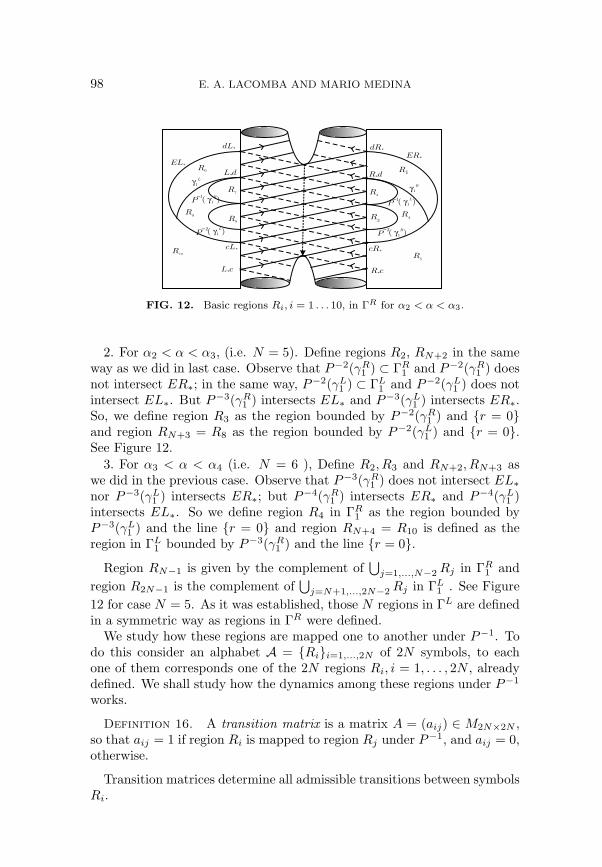
FIG. 12. Basic regions Ri, i = 1 . . . 10, in ΓR for α2 < α < α3.

2. For α2 < α < α3, (i.e. N = 5). Define regions R2, RN+2 in the sameway as we did in last case. Observe that P−2(γR

1 ) ⊂ ΓR1 and P−2(γR

1 ) doesnot intersect ER∗; in the same way, P−2(γL

1 ) ⊂ ΓL1 and P−2(γL

1 ) does notintersect EL∗. But P−3(γR

1 ) intersects EL∗ and P−3(γL1 ) intersects ER∗.

So, we define region R3 as the region bounded by P−2(γR1 ) and {r = 0}

and region RN+3 = R8 as the region bounded by P−2(γL1 ) and {r = 0}.

See Figure 12.3. For α3 < α < α4 (i.e. N = 6 ), Define R2, R3 and RN+2, RN+3 as

we did in the previous case. Observe that P−3(γR1 ) does not intersect EL∗

nor P−3(γL1 ) intersects ER∗; but P−4(γR

1 ) intersects ER∗ and P−4(γL1 )

intersects EL∗. So we define region R4 in ΓR1 as the region bounded by

P−3(γL1 ) and the line {r = 0} and region RN+4 = R10 is defined as the

region in ΓL1 bounded by P−3(γR

1 ) and the line {r = 0}.Region RN−1 is given by the complement of

⋃j=1,...,N−2 Rj in ΓR

1 andregion R2N−1 is the complement of

⋃j=N+1,...,2N−2 Rj in ΓL

1 . See Figure12 for case N = 5. As it was established, those N regions in ΓL are definedin a symmetric way as regions in ΓR were defined.

We study how these regions are mapped one to another under P−1. Todo this consider an alphabet A = {Ri}i=1,...,2N of 2N symbols, to eachone of them corresponds one of the 2N regions Ri, i = 1, . . . , 2N , alreadydefined. We shall study how the dynamics among these regions under P−1

works.

Definition 16. A transition matrix is a matrix A = (aij) ∈ M2N×2N ,so that aij = 1 if region Ri is mapped to region Rj under P−1, and aij = 0,otherwise.

Transition matrices determine all admissible transitions between symbolsRi.


Definition 17. The transition graph GA, associated to a transitionmatrix A is the directed graph with 2N different vertices, which by sim-plicity are denoted by i, i = 1, . . . , 2N and some directed arrows. We havea directed arrow from vertex i to vertex j if aij = 1; in case aij = 0, thereis no connection from vertex i to vertex j.

Our objective is to determine a transition matrix A, which describes thedynamics of the regions Ri, for a given range of values of the parameterand its associated transition graph. This permits to know the dynamics ofthe orbit beginning in a given region in terms of its sequence of binary andsimultaneous binary collisions. We will use all of the previously obtainedinformation

Theorem 18. Transition matrices for the symmetric collinear four bodyproblem are given by matrices of the form

A =(

C DD C

)∈ M2N×2N ,

where

C =

0 . . . 0 0 0...

. . . 0 0 00 0 0 0 00 0 0 0 01 0 . . . 0 1

, D =

0 1 0 . . . 0... 0

. . . 0 0... 0 0 1 10 0 0 1 10 . . . . . . 0 0

∈ MN×N

and N = 4 corresponds to 0 < α < α1, N = 5 corresponds to α2 < α < α3

and N = 6 corresponds to α3 < α < α4.

Proof. The pullback of region RN is obtained as follows. The argumentfor any of the three cases is the same. So we consider any of N = 4, 5, or6. All considered points lie in RN . The pullback of a point in RN nearcR∗ pass near R∗c and the pullback of a point in the region, close to ER∗,must be close to R∗d. Analogously, points close to dR∗, under P−1, go topoints near R∗d. So, P−1(RN ) intersects R1 and RN . Pullbacks for theothers regions are determined in a similar way.

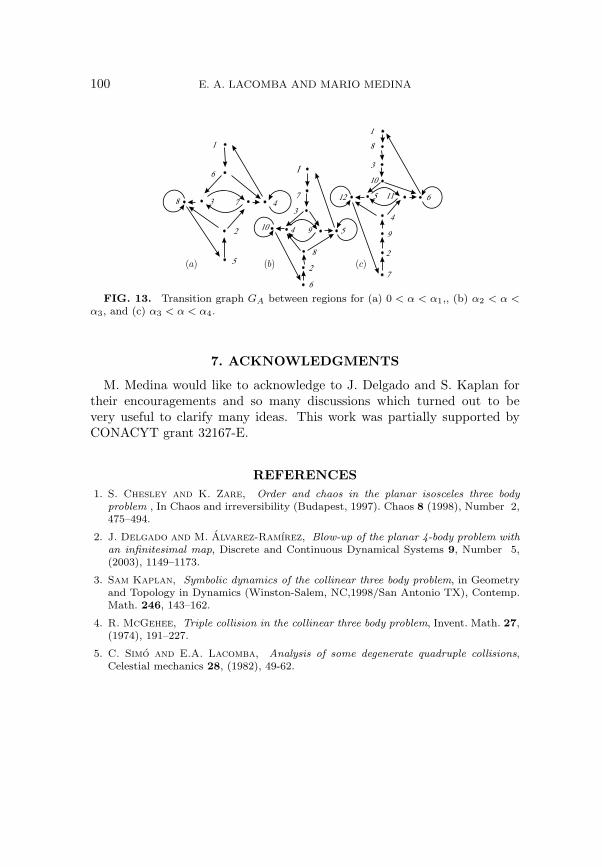
Corollary 19. Transition graphs between regions are given in Figure13.

The proof follows from Theorem 18 and is omitted.Observe that symmetries appearing in all transition matrices and their

associated transition graphs reflect the geometric symmetries of the colli-near configuration.


7

2

510

3

8

4 9

6

13

10

9

612

4

5 11

2

7

8

1

1

5

48

6

2

3 7

( )a ( )b ( )c

FIG. 13. Transition graph GA between regions for (a) 0 < α < α1,, (b) α2 < α <α3, and (c) α3 < α < α4.

7. ACKNOWLEDGMENTS

M. Medina would like to acknowledge to J. Delgado and S. Kaplan fortheir encouragements and so many discussions which turned out to bevery useful to clarify many ideas. This work was partially supported byCONACYT grant 32167-E.

REFERENCES1. S. Chesley and K. Zare, Order and chaos in the planar isosceles three body

problem , In Chaos and irreversibility (Budapest, 1997). Chaos 8 (1998), Number 2,475–494.

2. J. Delgado and M. Alvarez-Ramırez, Blow-up of the planar 4-body problem withan infinitesimal map, Discrete and Continuous Dynamical Systems 9, Number 5,(2003), 1149–1173.

3. Sam Kaplan, Symbolic dynamics of the collinear three body problem, in Geometryand Topology in Dynamics (Winston-Salem, NC,1998/San Antonio TX), Contemp.Math. 246, 143–162.

4. R. McGehee, Triple collision in the collinear three body problem, Invent. Math. 27,(1974), 191–227.

5. C. Simo and E.A. Lacomba, Analysis of some degenerate quadruple collisions,Celestial mechanics 28, (1982), 49-62.

Symbolic dynamics in the symmetric collinear four-body problem

Documents