Symbolic Computation of Recursion Operators for Nonlinear Differential-Difference Equations

SYMBOLIC COMPUTATION OF RECURSION OPERATORS FOR

NONLINEAR DIFFERENTIAL-DIFFERENCE EQUATIONS

Ünal Göktaş1*

and Willy Hereman2

1Department of Computer Engineering, Turgut Özal University

Keçiören, Ankara 06010, Turkey.

[email protected] 2Department of Mathematical and Computer Sciences, Colorado School of Mines

Golden, Colorado 80401-1887, U.S.A.

[email protected]

Abstract- An algorithm for the symbolic computation of recursion operators for sys-

tems of nonlinear differential-difference equations (DDEs) is presented. Recursion op-

erators allow one to generate an infinite sequence of generalized symmetries. The exis-

tence of a recursion operator therefore guarantees the complete integrability of the

DDE. The algorithm is based in part on the concept of dilation invariance and uses our

earlier algorithms for the symbolic computation of conservation laws and generalized

symmetries.

The algorithm has been applied to a number of well-known DDEs, including the Kac-

van Moerbeke (Volterra), Toda, and Ablowitz-Ladik lattices, for which recursion opera-

tors are shown. The algorithm has been implemented in Mathematica, a leading com-

puter algebra system. The package DDERecursionOperator.m is briefly discussed.

Keywords- Conservation Law, Generalized Symmetry, Recursion Operator, Nonlinear

Differential-Difference Equation

1. INTRODUCTION

A number of interesting problems can be modeled with nonlinear differential-

difference equations (DDEs) [1]-[3], including particle vibrations in lattices, currents in

electrical networks, and pulses in biological chains. Nonlinear DDEs also play a role in

queuing problems and discretizations in solid state and quantum physics, and arise in

the numerical solution of nonlinear PDEs.

The study of complete integrability of nonlinear DDEs largely parallels that of

nonlinear partial differential equations (PDEs) [4]-[7]. Indeed, as in the continuous case,

the existence of large numbers of generalized (higher-order) symmetries and conserved

densities is a good indicator for complete integrability. Albeit useful, such predictors do

not provide proof of complete integrability. Based on the first few densities and symme-

tries, quite often one can explicitly construct a recursion operator which maps higher-

order symmetries of the equation into new higher-order symmetries. The existence of a

recursion operator, which allows one to generate an infinite set of such symmetries step-

by-step, then confirms complete integrability.

There is a vast body of work on the complete integrability of DDEs. Consult,

e.g., [5, 8] for additional references. In this article we describe an algorithm to symboli-

cally compute recursion operators for DDEs. This algorithm builds on our related work

for PDEs and DDEs [9]-[11] and work by Oevel et al [12] and Zhang et al [13].

In contrast to the general symmetry approach in [5], our algorithms rely on spe-

cific assumptions. For example, we use the dilation invariance of DDEs in the construc-

tion of densities, higher-order symmetries, and recursion operators. At the cost of gene-

rality, our algorithms can be implemented in major computer algebra systems.

Our Mathematica package InvariantsSymmetries.m [14] computes densities

and generalized symmetries, and therefore aids in automated testing of complete inte-

grability of semi-discrete lattices. Our new Mathematica package DDERecursionOpe-

rator.m [15] automates the required computations for a recursion operator.

The paper is organized as follows. In Section 2, we present key definitions, ne-

cessary tools, and prototypical examples, namely the Kac-van Moerbeke (KvM) [16]

and Toda [17, 18] lattices. An algorithm for the computation of recursion operators is

outlined in Section 3. Usage of our package is demonstrated on an example in Section 4.

Section 5 covers two additional examples, namely the Ablowitz-Ladik (AL) [19] and

RelativisticToda (RT) [20] lattices. Concluding remarks about the scope and limitations

of the algorithm are given in Section 6.

2. KEY DEFINITIONS

2.1. Definition

A nonlinear DDE is an equation of the form

,,...),,(..., 11 nnnn uuuFu (1)

where nu and F are vector-valued functions with N components. The subscript n cor-

responds to the label of the discretized space variable; the dot denotes differentiation

with respect to the continuous time variable .t Throughout the paper, for simplicity we

denote the components of nu by ,...),,( nnn wvu and write ),( nuF although F typically

depends on nu and a finite number of its forward and backward shifts. We assume that

F is polynomial with constant coefficients. No restrictions are imposed on the shifts or

the degree of nonlinearity in .F

2.2. Example

The Kac-van Moerbeke (KvM) lattice [16], also known as the Volterra lattice,

,)( 11 nnnn uuuu (2)

arises in the study of Langmuir oscillations in plasmas, population dynamics, etc.

2.3. Example

One of the earliest and most famous examples of completely integrable DDEs is

the Toda lattice [17,18],

,)exp()exp( 11 nnnnn yyyyy (3)

where ny is the displacement from equilibrium of the nth particle with unit mass under

an exponential decaying interaction force between nearest neighbors. With the change

of variables, ),exp(, 1 nnnnn yyvyu due to Flaschka [21], lattice (3) can be writ-

ten in polynomial form [22]

.)(, 11 nnnnnnn uuvvvvu (4)

2.4. Definition

A DDE is said to be dilation invariant if it is invariant under a scaling (dilation)

symmetry.

2.5. Example

Lattice (2) is invariant under ),,(),( 1

nn utut where is an arbitrary

scaling parameter.

2.6. Example

Equation (4) is invariant under the scaling symmetry

,),,(),,( 21

nnnn vutvut (5)

where is an arbitrary scaling parameter.

2.7. Definition

We define the weight, ,w of a variable as the exponent in the scaling parameter

which multiplies the variable. As a result of this definition, t is always replaced by

t and .1)D()dtd( tww In view of (5), we have ,1)( nuw and 2)( nvw for the

Toda lattice.

Weights of dependent variables are nonnegative, integer or rational numbers,

and independent of .n For example, ),()()( 11 nnn uwuwuw etc.

2.8. Definition

The rank of a monomial is defined as the total weight of the monomial. An ex-

pression is uniform in rank if all of its terms have the same rank.

2.9. Example

In the first equation of (4), all the monomials have rank 2; in the second equation

all the monomials have rank 3. Conversely, requiring uniformity in rank for each equa-

tion in (4) allows one to compute the weights of the dependent variables (and thus the

scaling symmetry) with elementary linear algebra. Indeed,

),()(1)(),(1)( nnnnn vwuwvwvwuw (6)

yields

,2)(,1)( nn vwuw (7)

which is consistent with (5).

Dilation symmetries, which are Lie-point symmetries, are common to many lat-

tice equations. Polynomial DDEs that do not admit a dilation symmetry can be made

scaling invariant by extending the set of dependent variables with auxiliary parameters

with appropriate scales.

2.10. Definition

A scalar function )( nn u is a conserved density of (1) if there exists a scalar

function ),( nnJ u called the associated flux, such that [23]

0D nnt J (8)

is satisfied on the solutions of (1).

In (8), we used the (forward) difference operator,

,)ID( 1 nnnn JJJJ (9)

where D denotes the up-shift (forward or right-shift) operator, ,D 1 nn JJ and I is the

identity operator.

The operator takes the role of a spatial derivative on the shifted variables as

many DDEs arise from discretization of a PDE in 11 variables. Most, but not all, den-

sities are polynomial in .nu

2.11. Example

The first three density-flux pairs [11] for (2) are

,),ln( 1

)0()0(

nnnnn uuJu (10)

,, 1

)1()1(

nnnnn uuJu (11)

).(,2

111

)2(

1

2)2(

nnnnnnnnn uuuuJuuu (12)

2.12. Example

The first four density-flux pairs [22] for (4) are

,),ln( )0()0(

nnnn uJv (13)

,, 1

)1()1(

nnnn vJu (14)

,,2

11

)2(2)2(

nnnnnn vuJvu (15)

.),(3

1 2

111

)3(

1

3)3(

nnnnnnnnnn vvuuJvvuu (16)

The densities in (13)-(16) are uniform of ranks 0 through 3, respectively. The

corresponding fluxes are also uniform in rank with ranks 1 through 4, respectively. In

general, if in (8) Rn rank then ,1rank RJ n since .1)D( tw The various piec-

es in (8) are uniform in rank. Since (8) holds on solutions of (1), the conservation law

‘inherits’ the dilation symmetry of (1).

Consult [22] for our algorithm to compute polynomial conserved densities and

fluxes, where we use (4) to illustrate the steps. Non-polynomial densities (which are

rare) can be computed by hand or with the method given in [8].

2.13. Definition

A vector function )( nuG is called a generalized (higher-order) symmetry of (1)

if the infinitesimal transformation Guu nn leaves (1) invariant up to order .

Consequently, G must satisfy [23]

])[(D t GuFG n (17)

on solutions of (1). ])[( GuF n is the Fréchet derivative of F in the direction of .G

For the scalar case ),1( N the Fréchet derivative in the direction of G is com-

puted as

,D|)(])[( 0 Gu

FGuFGuF k

k kn

nn

(18)

which defines the Fréchet derivative operator

.D)( k

k kn

nu

FuF

(19)

For the vector case with two components nu and ,nv the Fréchet derivative op-

erator is

.

DD

DD

)(22

11

k

k

knk

k

kn

k

k

knk

k

knn

v

F

u

F

v

F

u

F

uF (20)

Applied to ,),( T

21 GGG where T is transpose, one gets

.2,1,DD])[( 21

iGv

FG

u

FF k

k kn

ik

k kn

i

ni Gu (21)

In (18) - (21), summation is over all positive and negative shifts (including the term

without shift, i.e., 0).k For 0,k times).(D...DDDk k Similarly, for 0k

the down-shift operator -1D is applied repeatedly. The generalization of (20) to N com-

ponents should be obvious.

2.14. Example

The first two symmetries [11] of (2) are

),( 11

)1(

nnn uuuG (22)

.)()( 121211

)2(

nnnnnnnnnn uuuuuuuuuuG (23)

These symmetries are uniform in rank (rank 2 and 3, respectively). Symmetries of ranks

0 and 1 are both zero.

2.15. Example

The first two non-trivial symmetries [24] of (4),

,)( 1

1)1(

nnn

nn

uuv

vvG (24)

,)(

)()(

11

22

1

111)2(

nnnnn

nnnnnn

vvuuv

uuvuuvG (25)

are uniform in rank. For example, 3rank )2(

1 G and .4rank )2(

2 G The symmetries of

lower ranks are trivial.

An algorithm to compute polynomial generalized symmetries is described in de-

tail in [24].

3. COMPUTATION OF RECURSION OPERATORS

3.1. Definition

A recursion operator connects symmetries

,)()( jsjGG (26)

where ...,,2,1j and s is the gap length. The symmetries are linked consecutively if

.1s This happens in most, but not all, cases. For N component systems, is an

NN x matrix operator.

The defining equation for [6, 23] is

,0)()()(,D t

nnn

tuFuFFuF (27)

where the bracket , denotes the commutator of operators and the composition of

operators. The operator )( nuF was defined in (20). F is the Fréchet derivative of

in the direction of .F For the scalar case, the operator is often of the form

),(D)I,,D,)ID(()( -11

nn uVuU (28)

and in that case

.)D()(D k

knkkn

k

k u

VFUV

u

UFF

(29)

For the vector case and the examples under consideration, the elements of the NN x

operator matrix are of the form ).(D)I,,D,)ID(()( -11

nijijnijij VU uu Thus,

for the two-component case [7]

.)D()D(

)(D)(D

2

k

1

k

21

kn

ij

k

ijij

kn

ij

k

ijij

ijij

kn

ijk

k

ijij

kn

ijk

k

ij

v

VFU

u

VFU

Vv

UFV

u

UFF

(30)

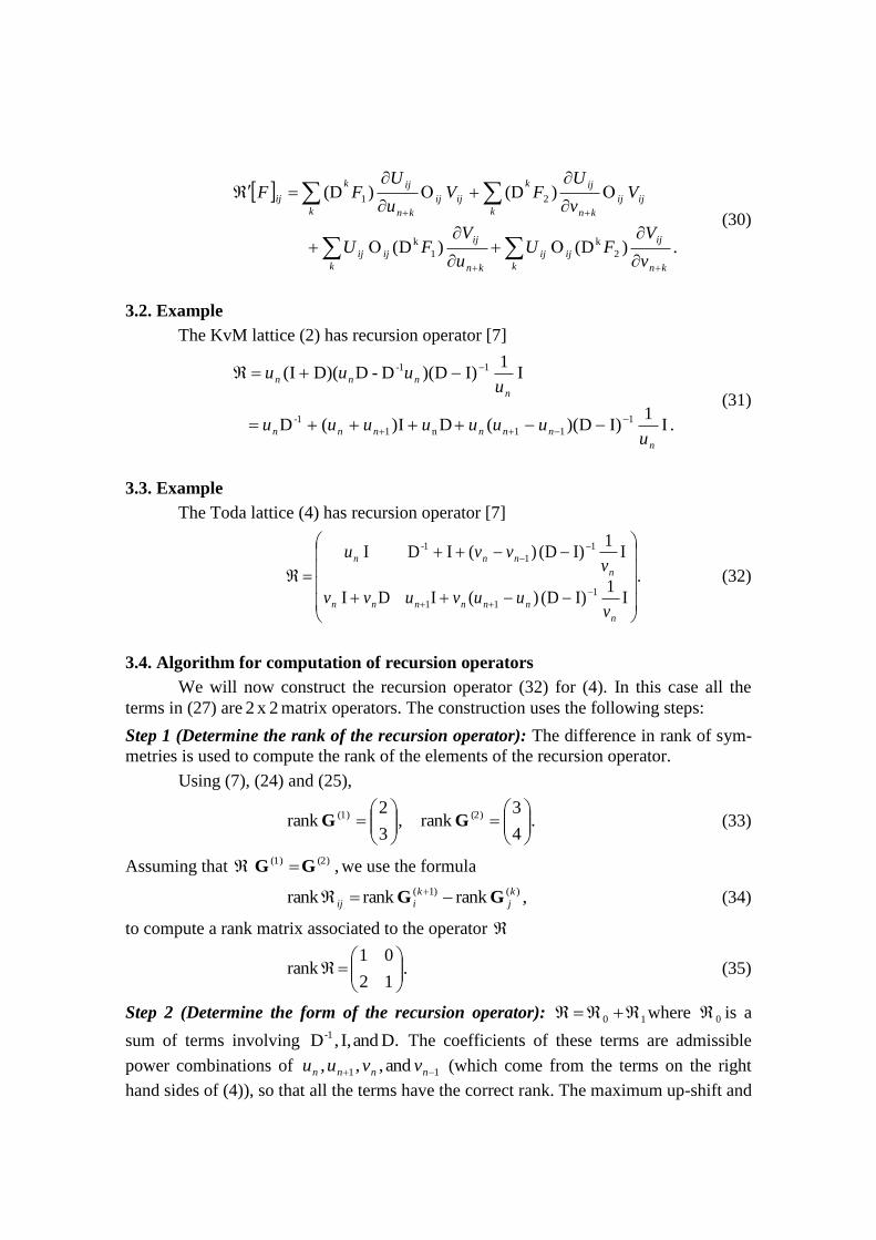
3.2. Example

The KvM lattice (2) has recursion operator [7]

. I1

)ID)((DI)(D

I1

)ID)(D-D)(DI(

1

11n1

1-

11-

n

nnnnnn

n

nnn

uuuuuuuu

uuuu

(31)

3.3. Example

The Toda lattice (4) has recursion operator [7]

.

I1

)ID()(IDI

I1

)ID()(IDI

1

11

1

1

1-

n

nnnnnn

n

nnn

vuuvuvv

vvvu

(32)

3.4. Algorithm for computation of recursion operators

We will now construct the recursion operator (32) for (4). In this case all the

terms in (27) are 2x2 matrix operators. The construction uses the following steps:

Step 1 (Determine the rank of the recursion operator): The difference in rank of sym-

metries is used to compute the rank of the elements of the recursion operator.

Using (7), (24) and (25),

.4

3rank,

3

2rank (2)(1)

GG (33)

Assuming that ,(2)(1) GG we use the formula

,rankrankrank )()1( k

j

k

iij GG (34)

to compute a rank matrix associated to the operator

.12

01rank

(35)

Step 2 (Determine the form of the recursion operator): 10 where 0 is a

sum of terms involving D.and,I,D-1 The coefficients of these terms are admissible

power combinations of 11 and,,, nnnn vvuu (which come from the terms on the right

hand sides of (4)), so that all the terms have the correct rank. The maximum up-shift and

down-shift operator that should be included can be determined by comparing two con-

secutive symmetries. Indeed, if the maximum up-shift in the first symmetry is ,pnu and

the maximum up-shift in the next symmetry is ,rpnu then the associated piece that

goes into 0 must have .D,...,D,D r2 The same line of reasoning determines the mini-

mum down-shift operator to be included. So, in our example

,)()(

)()(

220210

120110

0

(36)

with

,I)()( 121110 nn ucuc

,ID)( 4

-1

3120 cc

D,)(

I)()(

14113

2

112111

2

10

918

2

1716

2

5210

nnnnnn

nnnnnn

vcvcucuucuc

vcvcucuucuc

(37)

.I)()( 11615220 nn ucuc

As in the continuous case [10], 1 is a linear combination (with constant coeffi-

cients jkc~ of sums of all suitable products of symmetries and covariants (Fréchet deriva-

tives of conserved densities) sandwiching .)ID( 1 Hence,

,)ID(~ )(1)( k

n

j

j k

jkc G (38)

where denotes the matrix outer product, defined as

.)ID()ID(

)ID()ID()ID(

)(

2,

1)(

2

)(

1,

1)(

2

)(

2,

1)(

1

)(

1,

1)(

1)(

2,

)(

1,

1

)(

2

)(

1

k

n

jk

n

j

k

n

jk

n

j

k

n

k

nj

j

GG

GG

G

G

(39)

Only the pair ),( )0()1(

nG can be used, otherwise the ranks in (35) would be exceeded.

Using (13) and (21), we compute

.I1

0)0(

n

nv

(40)

Therefore, using (38) and renaming 10~c to ,17c

.

I1

)ID()(0

I1

)ID()(0

1

117

1

117

1

n

nnn

n

nn

vuuvc

vvvc

(41)

Adding (36) and (41), we obtain

.2221

1211

10

(42)

Step 3 (Determine the unknown coefficients): All the terms in (27) need to be com-

puted. Referring to [7] for details, the result is:

.1and,1

,0

1716149431

151312111087652

ccccccc

cccccccccc (43)

Substituting these constants into (42) finally gives

.

I1

)ID()(IDI

I1

)ID()(IDI

1

11

1

1

1-

n

nnnnnn

n

nnn

vuuvuvv

vvvu

(44)

One can readily verify that )2()1(GG with )1(

G in (24) and )2(G in (25).

4. THE MATHEMATICA PACKAGE

To use the code, first load the Mathematica package DDERecursionOpera-

tor.m using the command

];m".onOperatorDDERecursi["Get :=In[2]

Proceeding with the KvM lattice (2) as an example, call the function DDERe-

cursionOperator (which is part of the package) :

&}}} t])n, + u[1 t]u[n, + t]u[n, t]n, + (-u[-1 t}]{n, t],[#1/u[n, + t])n, + u[1 +

t](u[n, #1 + t]u[n, 1}] {n, ift[#1,DiscreteSh+ t]u[n, 1}]- {n, eShift[#1,{{{Discret =Out[3]

. 1}- Weight[u]-1,- {Weight[t]

is )(sequation theof symmetryDilation :dilation::Weight

] t}{n, {u},

0}, == t]))1, -u[n - t]1, +(u[n * t](u[n, - t] t],[{D[u[n, onOperatorDDERecursi :=In[3]

1-

n

Here .)ID( 1-1

n

The first part of the output (which we assign to R for later

use) is indeed the recursion operator given in (31).

First[%];R :=In[4]

Now using the first symmetry, generate the next symmetry by calling the func-

tion GenerateSymmetries (which is also part of the package):

t]}n,u[2 t]n,u[1 t]u[n,t]n,u[1 t]u[n,t]n,u[1 t]u[n,

t]u[n, t]n,u[-1-t]u[n, t]n,u[-1-t]u[n, t]n,u[-1 t]n,{-u[-2=Out[6]

1][[1]]try,firstsymme,mmetries[RGenerateSy: In[6]

t])};1,-u[n-t]1,(u[nt]{u[n,tryfirstsymme: In[5]

22

22

Evaluating the next five symmetries starting from the first one, can be done as

follows:

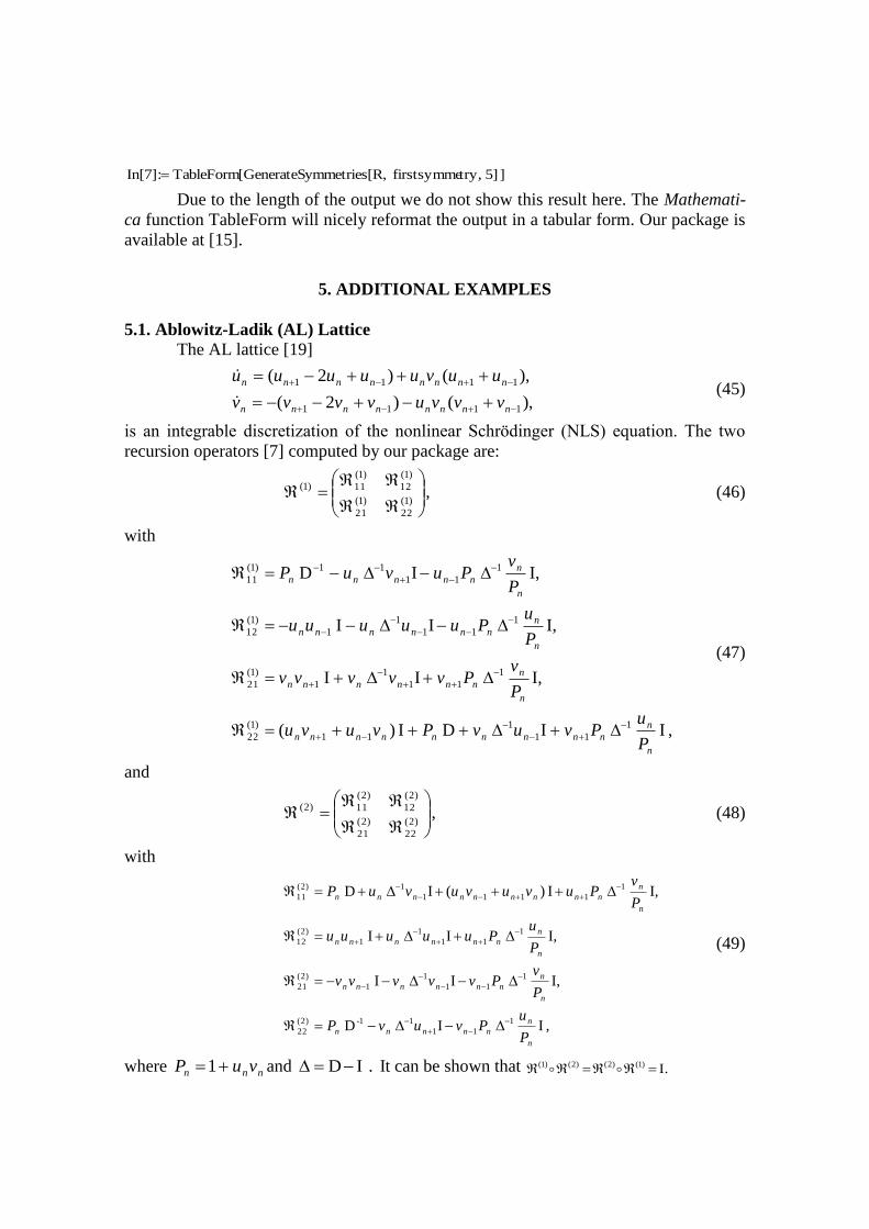
] 5] try,firstsymme ,mmetries[RGenerateSy[TableForm: In[7]

Due to the length of the output we do not show this result here. The Mathemati-

ca function TableForm will nicely reformat the output in a tabular form. Our package is

available at [15].

5. ADDITIONAL EXAMPLES

5.1. Ablowitz-Ladik (AL) Lattice

The AL lattice [19]

),()2(

),()2(

1111

1111

nnnnnnnn

nnnnnnnn

vvvuvvvv

uuvuuuuu

(45)

is an integrable discretization of the nonlinear Schrödinger (NLS) equation. The two

recursion operators [7] computed by our package are:

,)1(

22

)1(

21

)1(

12

)1(

11)1(

(46)

with

, IIDI)(

I,II

I,II

I,ID

1

11

1

11

)1(

22

1

11

1

1

)1(

21

1

11

1

1

)1(

12

1

11

11)1(

11

n

n

nnnnnnnnn

n

n

nnnnnn

n

n

nnnnnn

n

n

nnnnn

P

uPvuvPvuvu

P

vPvvvvv

P

uPuuuuu

P

vPuvuP

(47)

and

,)2(

22

)2(

21

)2(

12

)2(

11)2(

(48)

with

, IID

I,II

I,II

I,I)(ID

1

11

11-)2(

22

1

11

1

1

)2(

21

1

11

1

1

)2(

12

1

1111

1)2(

11

n

n

nnnnn

n

n

nnnnnn

n

n

nnnnnn

n

n

nnnnnnnnn

P

uPvuvP

P

vPvvvvv

P

uPuuuuu

P

vPuvuvuvuP

(49)

where nnn vuP 1 and . ID It can be shown that .I)1()2()2()1(

5.2. Relativistic Toda (RT) Lattice

The RT lattice [20] is given as

,)(),( 1111 nnnnnnnnnn vvuuuuuuvv (50)

and the recursion operator found by our package coincides with the one in [20]:

.

I1

)ID()(

I)(DD

ID

I1

)ID()(IDI

1

111

11

1-

1

1

1-

n

nnnnn

nnnnn

nn

n

nnnnn

n

uvvuuu

vuuuu

uu

uuuvvv

v

(51)

6. CONCLUDING REMARKS

The existence of a recursion operator is a corner stone in establishing the com-

plete integrability of nonlinear DDEs because the recursion operators allows one to

compute an infinite sequence of generalized symmetries.

Therefore, we presented an algorithm to compute recursion operators of nonli-

near DDEs with polynomial terms. The algorithm uses the scaling properties, conserva-

tion laws, and generalized symmetries of the DDE, but does not require the knowledge

of the bi-Hamiltonian operators. The algorithm has been implemented in Mathematica,

a leading computer algebra system. The package DDERecursionOperators.m uses In-

variantsSymmetries.m to compute the conservation laws and higher-order symmetries

of nonlinear DDEs.

The algorithm presented in this paper works for many nonlinear DDEs, includ-

ing the Kac-van Moerbeke (Volterra), modified Volterra, and Ablowitz-Ladik lattices,

as well as standard and relativistic Toda lattices. However, the algorithm does not allow

one to compute recursion operators for lattices due to Blaszak-Marciniak and Belov-

Chaltikian (see, e.g., [20] for references). An extension of the algorithm that would cov-

er these lattices is under investigation.

Acknowledgements- This material is based upon work supported by the National

Science Foundation (U.S.A.) under Grant No. CCF-0830783. J. A. Sanders, J.-P. Wang,

M. Hickman and B. Deconinck are gratefully acknowledged for valuable discussions.

7. REFERENCES

1. Y. B. Suris, (1999). Integrable discretizations for lattice systems: local equations of

motion and their Hamiltonian properties, Rev. Math. Phys., 11, 727-822.

2. Y. B. Suris, 2003. The Problem of Discretization: Hamiltonian Approach, Birkhäuser

Verlag, Basel, Switzerland.

3. G. Teschl, 2000. Jacobi Operators and Completely Integrable Nonlinear Lattices,

AMS Mathematical Surveys and Monographs, 72, AMS, Providence, RI.

4. M. J. Ablowitz and P. A. Clarkson, 1991. Solitons, Nonlinear Evolution Equations

and Inverse Scattering, London Math. Soc. Lecture Note Ser., 149, Cambridge Univ.

Press, Cambridge, U.K..

5. V. E. Adler, A. B. Shabat and R. I. Yamilov, (2000). Symmetry approach to the inte-

grability problem, Theor. And Math. Phys., 125, 1603-1661.

6. J. P. Wang, 1998. Symmetries and Conservation Laws of Evolution Equations, Ph.D.

Thesis, Thomas Stieltjes Institute for Mathematics, Amsterdam.

7. W. Hereman, J. A. Sanders, J. Sayers, and J. P. Wang, (2005). Symbolic computation

of polynomial conserved densities, generalized symmetries, and recursion operators for

nonlinear differential-difference equations, CRM Proceedings and Lecture Notes, 39,

133-148.

8. M. S. Hickman and W. A. Hereman, (2003). Computation of densities and fluxes of

nonlinear differential-difference equations, Proc. Roy. Soc. Lond. Ser. A, 459, 2705-

2729.

9. Ü. Göktaş and W. Hereman, (1997). Symbolic computation of conserved densities for

systems of nonlinear evolution equations, J. Symbolic Comput., 24, 591--621.

10. W. Hereman and Ü. Göktaş, 1999. Integrability Tests for Nonlinear Evolution Equa-

tions. Computer Algebra Systems: A Practical Guide, (M. Wester, ed.), Wiley, New

York, 211-232.

11. W. Hereman, Ü. Göktaş, M. D. Colagrosso and A. J. Miller, (1998). Algorithmic

integrability tests for nonlinear differential and lattice equations, Comput. Phys. Comm.,

115, 428-446.

12. W. Oevel, H. Zhang and B. Fuchssteiner, (1989). Mastersymmetries and multi-

Hamiltonian formulations for some integrable lattice systems, Progr. Theor. Phys., 81,

294-308.

13. H. Zhang, G. Tu, W. Oevel, and B. Fuchssteiner, (1991). Symmetries, conserved

quantities, and hierarchies for some lattice systems with soliton structure, J. Math.

Phys., 32, 1908-1918.

14. Ü. Göktaş and W. Hereman, 1997. Mathematica package InvariantsSymmetries.m

for the symbolic computation of conservation laws and generalized symmetries of non-

linear polynomial PDEs and differential-difference equations. Code is available at

http://library.wolfram.com/infocenter/MathSource/570.

15. Ü. Göktaş and W. Hereman, 2010. Mathematica package DDERecursionOperator.m

for the symbolic computation of recursion operators for nonlinear polynomial differen-

tial-difference equations. The Mathematica package is available at

http://inside.mines.edu/~whereman/software/DDERecursionOperator.

16. M. Kac and P. van Moerbeke, (1975). On an explicitly soluble system of nonlinear

differential equations related to certain Toda lattices, Adv. Math., 16, 160-169.

17. M. Toda, (1967). Vibration of a chain with nonlinear interaction, J. Phys. Soc. Ja-

pan, 22, 431-436.

18. M. Toda, 1993. Theory of Nonlinear Lattices, Berlin: Springer Verlag, 2nd

edition.

19. M. J. Ablowitz and J. F. Ladik, (1975). Nonlinear differential-difference equations,

J. Math. Phys., 16, 598-603.

20. R Sahadevan and S. Khousalya, (2003). Belov-Chaltikian and Blaszak-Marciniak

lattice equations: Recursion operators and factorization, J. Math. Phys., 44, 882-898.

21. H. Flaschka, (1974). The Toda lattice I. Existence of integrals, Phys. Rev. B, 9,

1924-1925.

22. Ü. Göktaş and W. Hereman, (1998). Computation of conserved densities for nonli-

near lattices, Physica D, 123, 425-436.

23. P. J. Olver, 1993. Applications of Lie Groups to Differential Equations, Grad. Texts

in Math., 107, New York: Springer Verlag.

24. Ü. Göktaş and W. Hereman, (1999). Algorithmic computation of higher-order sym-

metries for nonlinear evolution and lattice equations, Adv. Comput. Math., 11, 55-80.