Acta Appficandae Mathematicae 1, 43-77. 0167-8019/83/0011-043505.25. 43 Copyright 1983 D. Reidel Publishing Co. Symbolic Computations in Applied Differential Geometry P. K. H. GRAGERT, P. H. M. KERSTEN, and R. MARTINI Department of Applied Mathematics, Twente University of Technology, PO Box 217, 7500 AE Enschede, The Netherlands (Received: 4 November 1982) Abstract. The main aim of this paper is to contribute to the automatic calculations in differential geometry and its applications, with emphasis on the prolongation theory of Estabrook and Wahlquist, and the calculation of invariance groups of exterior differential systems. A large number of worked examples have been included in the text to demonstrate the concrete manipulations in practice. In the appendix, a list of programs discussed in the paper is added. AMS (MOS) subject classifications (1980). 35 Partial Differential Equations, 53 Differential Geometry, 68 Computer Science. Key words. Symbolic computations, differential geometry, prolongation theory, exterior differential calculus, exterior differential systems, partial differential equations, invariance groups O. Introduction The impact of the computer on mathematics and its related fields is well-known. For instance, we are all familiar with its applications to numerical analysis, which started some decades ago. Its utility has also been proved in discrete mathematics, number theory and algebra (finite groups). Perhaps, less well-known is the recent progress of the application of symbolic calculations in the more continuous parts of mathematics, such as mathematical analysis, differential equations, differential geometry and its applications in theoreti- cal physics. In this context, we mention some outstanding results: the Risch algorithm to calculate indefinite integrals [17] and the program package SHEEP for formula manipulation, primarily in General Relativity [6]. The main aim of this paper is to contribute to the automatic calculations in dif- ferential geometry and its applications, with emphasis on the prolongation theory of Estabrook and Wahlquist [4, 5], and the calculations of invariance groups of exterior differential systems [7, 10]. A second aim is to encourage the reader to use symbolic calculations in his own field of interest. In contrast to the strategy of most papers related to symbolic calculations, which only discuss the theory and give final results of computations, we shall present by worked examples the explicit manipulations which have to be carried out in order to get to the results. An obvious but nonnegligible circumstance is the fact that, due to

Symbolic Computation and Automated Reasoning in Differential Geometry
Jun 29, 2015
Welcome message from author
This document is posted to help you gain knowledge. Please leave a comment to let me know what you think about it! Share it to your friends and learn new things together.
Transcript

Acta Appficandae Mathematicae 1, 43-77. 0167-8019/83/0011-043505.25. 43 Copyright �9 1983 D. Reidel Publishing Co.
Symbolic Computations in Applied Differential Geometry
P. K. H. G R A G E R T , P. H. M. K E R S T E N , and R. M A R T I N I Department of Applied Mathematics, Twente University of Technology, PO Box 217, 7500 AE Enschede, The Netherlands
(Received: 4 November 1982)
Abstract. The main aim of this paper is to contribute to the automatic calculations in differential geometry and its applications, with emphasis on the prolongation theory of Estabrook and Wahlquist, and the calculation of invariance groups of exterior differential systems. A large number of worked examples have been included in the text to demonstrate the concrete manipulations in practice. In the appendix, a list of programs discussed in the paper is added.
AMS (MOS) subject classifications (1980). 35 Partial Differential Equations, 53 Differential Geometry, 68 Computer Science.
Key words. Symbolic computations, differential geometry, prolongation theory, exterior differential calculus, exterior differential systems, partial differential equations, invariance groups
O. Introduction
The impact of the computer on mathematics and its related fields is well-known. For instance, we are all familiar with its applications to numerical analysis, which started some decades ago. Its utility has also been proved in discrete mathematics, number theory and algebra (finite groups).
Perhaps, less well-known is the recent progress of the application of symbolic calculations in the more continuous parts of mathematics, such as mathematical analysis, differential equations, differential geometry and its applications in theoreti- cal physics. In this context, we mention some outstanding results: the Risch algorithm to calculate indefinite integrals [17] and the program package SHEEP for formula manipulation, primarily in General Relativity [6].
The main aim of this paper is to contribute to the automatic calculations in dif- ferential geometry and its applications, with emphasis on the prolongation theory of Estabrook and Wahlquist [4, 5], and the calculations of invariance groups of exterior differential systems [7, 10]. A second aim is to encourage the reader to use symbolic calculations in his own field of interest.
In contrast to the strategy of most papers related to symbolic calculations, which only discuss the theory and give final results of computations, we shall present by worked examples the explicit manipulations which have to be carried out in order to get to the results. An obvious but nonnegligible circumstance is the fact that, due to

44 P . K . H . GRAGERT ET AL.
the use of symbolic calculations, one may carry out easy, although 'long and tedious'
calculations with the computer, thus avoiding lots of elementary mistakes, such as wrong signs, missing brackets, omitted symbols, etc.
There are several systems designed for symbolic calculations, e.g., FORMAC, SAC, MACSYMA, REDUCE, and we have chosen the language REDUCE [3] as a basis for our developments. It may be implemented on any computer system support- ting LISP [14] and it is cheap and easily available and, consequently, widespread. Last, but not least, we are charmed by the interactive facilities of REDUCE.
PLAN OF THE ARTICLE
Essentially, the paper consists of three parts. First, in order to become more familiar with REDUCE, some typical symbolic calculations are given. The second part is concerned with the basic manipulations of vector fields and differential forms (exterior differential calculus). The third part describes the application to infinitesimal sym- metries of exterior differential systems. In the appendix, a list of REDUCE procedures of the described material is included.
Before discussing the three parts in more detail, we shall make some general remarks relevant for all worked examples in each section.
(1) In the examples, a terminal session with the computer is reproduced in printout form.
(2) Input lines always begin with a '*', which is the prompt character of REDUCE, indicating that the system is waiting for a command, while the command itself is written in small letters.
(3) Output from the system is printed in capital letters. (4) Results of commands terminated by a ';' are printed. (5) Results of commands terminated by a '$' are not printed. (6) On each separate input line text following a '~ ' is ignored by REDUCE, and
therefore used as a means of including comment. (7) In input, the parentheses of functions with a single argument are not required
and, therefore, often omitted. In Section 1, three examples illustrating the capabilities of REDUCE are presented:
(a) a procedure for finite Taylor series expansions, which is applied to concrete cases; (b) the integration package; and (c) matrix calculations related to the theory of Lie algebras.
In Section 2 an implementation of differential geometric objects and their operations are described. The concepts of exterior differential calculus are succes- sively expounded. Keywords are: representation of differential forms and vector fields, exterior product, exterior derivative, commutator of vector fields, inner product of vector fields and forms and Lie derivatives of forms.
Section 3 is concerned with the computation of infinitesimal symmetries of exterior differential systems, representing differential equations. Determination of these symmetries gives rise to overdetermined systems of partial differential equations.

SYMBOLIC COMPUTATIONS IN APPLIED DIFFERENTIAL GEOMETRY 45
These are derived by the machinery of the Section 2. In order to solve such systems,
frequently-occurring computations are automized. Further, some auxiliaries are developed. The procedure is illustrated by two examples. Finally, the complete algebra of the infinitesimal symmetries for the Lin-Reisner-Tsien equation is given.
1. Introduction to Symbolic Computations
By means of some examples, which are chosen such that they are still computable by hand, we shall give a sample of the interactive symbolic computations in REDUCE. All functions not explicitly described in this section are already available in the basic REDUCE system. We recommend that the reader without experience consult the R E D U C E Users' Manual [11]. Moreover, one has to be informed how to start a REDUCE session.
(A) TAYLOR SERIES
Our first example will be a P R O C E D U R E for finite Taylor series expansions. Here, two special system functions are used, one for differentiation and one for substitution.
d f( function ,variable)
This command differentiates 'function' with respect to 'variable'.
sub(x=pt, expression)
Every 'x' occurring in 'expression' is substituted by 'pt'.
Note: Only the simplest form of DF and SUB are introduced here. in order to illustrate the Taylor series expansions for various functions, we write
a P R O C E D U R E :
*procedure taylor(fn,x,pt,u);begln scalar fakt; * fakt :=I ; * return * sub(x=pt, fn)+ * for i:~l:n sum * sub(x=pt , fn : =d f (fn,x))* * (fakt : = fakt* (x-pt)/i) *end taylor; TAYLOR
The four parameters of the PROCEDURE TAYLOR have the following meaning: F N has to be a function, X represents the variable with respect to which the function F N is expanded about the point P T up to order N.
EXAMPLE 1.1. The Taylor series expansion T(X) of a rational function F(X) with two parameters a and b:
2X 2 + X + 1 F(X) = b X 2 + a X + 2
about 0 up to order three is constructed. Moreover, we give the rest R(X), i.e., R(X) = = F(X) - T(X) .
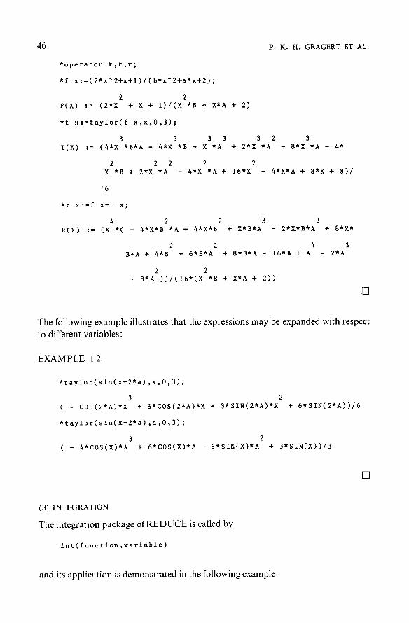
46 P. K. H. GRAGERT ET AL.
*operator f,t,r;
*f x:=(2*x'2+x+1)/(b*x^2+a*x+2);
2 2 F(X) := (2*X + X + I)/(X *B + X*A + 2)
*t x:=taylor(f x,x,0,3);
3 3 3 3 3 2 T(X) := (4*X *B*A - 4*X *B - X *A + 2*X *A
2 2 2 2 2 X *B + 2*X *A - 4*X *A + 16*X
16
*r x:=f x-t x;
4 2 2 3 R(X) := (X *( - 4*X*B *A + 4*X*B + X*B*A
2 2 B*A + 4*B - 6*B*A + 8*B*A - 16*B + A
2 2 + 8*A ))/(16*(X *B + X*A + 2))
3 - 8*X *A- 4*
- 4*X*A + 8*X + 8 ) /
2 - 2*X*B*A + 8*X*
4 3 - 2*A
[]
The following example illustrates that the expressions may be expanded with respect to different variables:
EXAMPLE 1.2,
*taylor(sin(x+2*a) ,x,0,3);
3 2 ( - COS(2*A)*X + 6*COS(2*A)*X - 3*SIN(2*A)*X + 6*SIN(2*A))/6
*taylor(s in(x+2*a) ,a,0,3);
3 2 ( - 4*COS(X)*A + 6*COS(X)*A- 6*SIN(X)*A + 3*SIN(X))/3
[]
(B) INTEGRATION
The integration package of REDUCE is called by
int( function ,variable)
and its application is demonstrated in the following example

SYMBOLIC COMPUTATIONS IN APPLIED DIFFERENTIAL GEOMETRY
EXAMPLE 1.3.
*h:=2ex*atan x/(l+x^2)A2; 4 2
H := (2*ATAN(X)*X)/(X + 2*X
H is now a function of x.
*hh:=int(h,x) ;
2 HH := (ATAN(X)*X - ATAN(X)
*h-df(hh,x);
0
*int(x*e^(x^2),x);
2 (x)
E /2
* I n t ( e ^ ( - x A 2 ) , x ) ;
+ 1)
2 2 2 (x) 2 (x) (x)
(E *INT((2*X )/E ,X) + X)/E
*on div;
2 + x)/(2*(x + I))
47
DIV is an output switch: each term gets its denominator. The last algebraic result is always stored under the name !*ANS.
[]
*!*ans; 2 2
(-x) 2 (x) E *X + INT((2*X )/E ,X)
(C) MATRIX C A L C U L A T I O N S
Matrix operations will be illustrated by calculations involving two different matrices.
EXAMPLE 1.4. The first matrix represents the adjoint matrix
ad(Ah + Bx + Cy)
of the Lie algebra M(2) with respect to the standard basis h, x, y, satisfying the com- mutator relations
[h,x]=ax, [h,y] = - 2 y , [x,y]=h.
Ah + Bx + Cy represents a 'general' element of ~1(2). For Convenience, the matrix
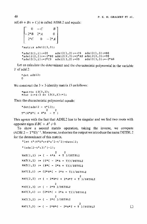
48 P. K. H. GRAGERT ET AL.
ad(Ah + Bx + Cy) is called ADSL2 and equals:
l_ 0 - C B 1 2*B 2*A 0
2"C 0 - 2*A
*matrlx ads12(3,3);
*adsl2(l,l):=0$ adsl2(l,2):=-C$ adsl2(l,3):=B$ *adsl2(2,1):=-2*B$ ads12(2,2):=2*A$ ads12(2,3):=05 *adsl2(3,1):=2*C$ ads12(3,2):=05 ads12(3,3):=-2*A$
Let us calculate the determinant and the characteristic polynomial in the variable T of adsl 2:
*det adsl2;
0
We construct the 3 x 3-identity matrix I3 as follows:
* m a t r i x i 3 ( 3 , 3 ) ; *for i:=1:3 do i3(i,i):=l;
Then the characteristic polynomial equals:
*det(adsl2 - t*13) ; 2 2
T* (4*B*C + 4*A - T )
This agrees with the fact that ADSL2 has to be singular and we find two roots with opposite signs if BC + A 2 # O.
To show a second matrix operation, taking the inverse, we compute (ADS1 2 - T*I3)- 1. Moreover, to shorten the output we introduce the name DETSL2 for the determinant of this matrix.
*let t*(4*b*c+4*a^2-t^2)=detsl2;
* (adsl2-t*13) ^(-I);
2 2 MAT(I,I) :- ( - 4*A + T )/DETSL2
MAT(I,2) := (C*( - 2*A - T))/DETSL2
MAT(I,3) :- (B*( - 2*A + T))/DETSL2
MAT(2,1) :- (2*B*( - 2*A - T))/DETSL2
2 MAT(2,2) := ( - 2*B*C + 2*A*T + T )/DETSL2
2 MAT(2,3) := ( - 2*B )/DETSL2
MAT(3,1) := (2"C*( - 2*A + T))/DETSL2
2 MAT(3,2) := ( - 2"C )/DETSL2
2 MAT(3,3) := ( - 2*B*C - 2*A*T + T )/DETSL2 []

SYMBOLIC COMPUTATIONS IN APPLIED DIFFERENTIAL GEOMETRY
Computations with matrix-polynomials are possible too and, comparable with the given examples.
49
of complication,
EXAMPLE 1.5. The second matrix represents the matrix of the Killing form of the Lie algebra with the following commutator table. Here the Lie product [x i, xj] is represented by LIE(i, j) and only nonzero commutators are printed.
This Lie algebra emerges in the determination of a 11-dimensional prolongation algebra of the Korteweg-de Vries equation [4, 8].
lie(l, 3) := x~5 lie(l, 4) := - x ^ 6 * M - x " 5 * L
lie(l, 5) := (x^4 + x ^ 3 * L - x ^ 2 ) / M
lie(l, 6) := - x^4 lie(2, 3) := - x^6 - x ^ 5 * M
lie(2, 4) := xA6*L lie(2, 5) := -- XA3*L + xA2
lie(2, 6) := (xA4*L + x ^ 3 * L ^2 -- x ^ 2 * L ) / M
lie(3, 4) := x^6 lie(3, 5) := - xA3 lie(3, 6) := (x^4 + x ^ 3 * L - x^2 - x * M ) / M
lie(4, 5) := x^2 + x * M
lie(4, 6) := - x A2*M + x*( -- M ^ 2 + L)
lie(8, 11):= - x^7
lie(9, 10) := x '7
The matrix C of the Killing form of the 6-dimensional sub-algebra spanned by x l , . . . , x 6 equals:
*matrix e(6,6);
After a declaration of a matrix, all elements are initialized to zero, therefore we have to give only the nonzero elements of C.
*c(l,l) : =2"m$ *c(2,2) :=2"m*I$ *c(1,3) :=c(3,1) :=-45 *c(4,4):=2*m*(-m^2+3*l)$ *c(5,6) :=c(6,5) :=-2"M5
We compute the determinant of C:
c(1,2):=C(2,1)-4"I$ c(2,3):=c(3,2):=2"m5 c(3,4):=c(4,3):=-2"m$ c(5,5):=45 c(6,6) := 2"(m^2 - 2"1)$
*det c;
2 6 4 2 2 3 64"M *(M - 12*M *L + 48"M *L - 64"L )
This result shows that this subalgebra is semisimple for almost all values of the para- meters L and M. []
50 P . K . H . GRAGERT ET AL.
2. Vector and Form Manipulations in REDUCE
Using the concepts of differential geometry in applied mathematics, we have to manipulate the vector fields and differential forms, which are 'living' on a differentiable manifold. All manipulations are essentially simple and straightforward, but doing computations by hand, in particular on high-dimensional spaces, the amount of labour grows rapidly and becomes rather tedious. Moreover, there is every chance that errors are introduced. For instance, a slip of the pen or a wrong sign is very likely. Manipulations with vector fields and forms are so systematic that they are very well suited for symbolic computations. In doing so only input, which is usually very short, has to be checked carefully.
In this section, almost all the computations are carried out with respect to a local coordinate system for an n-dimensional manifold M. So, in fact, we assume that M is a domain U of the Euclidean space R". All objects are assumed to be infinitely differentiable.
0-FORMS
The ring of all functions on U will be denoted by d~ 0-forms on U are identified with elements of d~
The algebraic mode of REDUCE already contains all tools to manipulate within the ring ~'~ In practice, the first problem to solve is to introduce local coordinates in a flexible way. The coordinates should be introduced such that indicial calculation is allowed and also such that a user may give them convenient names. This problem is solved by using the algebraic operator VNAT (natural variables), where VNAT(1), VNAT(2), . . . , VNAT(n) represents a coordinate system of U. The name of the ith coordinate may be changed into another, more suitable name by: VNAT(i) := 'name';
EXAMPLE 2.1. The coordinates ought to be x, y, z and ul , •2" This is introduced to REDUCE by:
*d!@dlf:=5$ *vnat l:=x$ vnat 2:=y$ vnat 3:=z$ *operator u; vnat 4:=u I; vnat 5:=u 2 5
VNAT(4) := U([)
Note: U(i) is used instead o f u i . []
Now let us define two functions f(1) and f(2), add and substract them, and let f(3) be the product o f f ( l ) and f(2).
EXAMPLE 2.2
*operator f; *f l:=for i:=1:5 sum i*vnat i;

SYMBOLIC COMPUTATIONS IN APPLIED DIFFERENTIAL GEOMETRY 51
F(1) := 4"O(i) + 5*U(2) + X + 2*Y + 3*Z
*f 2:=sin(vnat l+vnat 4)+3*(l+vnat(1)'2); 2
F(2) := SIN(U(1) + X) + 3*X + 3
An alternative way of input for f(2) is'
*f 2:=sln(x+u i)+3"(I+x'2)$
Any 'mixed form' of input is allowed too, and yields the same result.
*f l+f 2; 2
4*U(I) + 5*0(2) + SIN(U(1) + X) + 3*X + X + 2*Y + 3*Z + 3
*f l-f 2; 2
4"O(i) + 5*U(2) - SIN(U(1) + X) - 3*X + X + 2*Y + 3*Z - 3
*f 3:=f l*f 21
2 F(3) := 4*U(1)*SIN(U(1) + X) + 12*U(1)*X + 12"O(I) + 5*0(2)
2 *SIN(U(1) + X) + 15*0(2)*X + 15"O(2) + SIN(U(1) + X
3 )*X + 2*SIN(U(1) + X)*Y + 3*SIN(U(1) + X)*Z + 3*X
2 2 + 6*X *Y + 9*X *Z + 3*X + 6*Y + 9*Z
Here the construction off ( l ) shows the advantage of indicial calculations. []
Note: Observe that the examples show different ways of giving names.
I -FORMS
The set of 1-forms on the domain U is denoted by d~(U). Ifx 1 , x2, .. . , x is a coordi- nate system of U, then:
BF(1) = { dxl ,dx 2 . . . . . dx}
is a basis for the ~/~ ~r A general 1-form can be written in the form:
u = a ldx l + a 2dx 2 + . . . + a d x ,
where al, a 2 . . . . . a are elements of dO(u). In REDUCE, we represent the basis 1-forms by WEDGE(i), where WEDGE has
to be declared an algebraic operator.
EXAMPLE 2.2. Fixing the dimension of U to 3 and introducing coordinates X1, X2 and X3, a general 1-form in REDUCE can be constructed with, e.g., an

52 P. K. H. GRAGERT ET AL.
algebraic opera to r A as follows:
*u:=for i:=1:3 sum a(i,xl,x2,x3)*wedge i;
U := A(I,XI,X2,X3)*WEDGE(1) + A(2,XI,X2,X3)*WEDGE(2) + A(3,
Xl ,X2 , X3)*WEDGE(3)
A more concrete 1 - form is:
*v : =x2*wedge ( I )-wedge(3) ;
V := X2*WEDGE(1) - WEDGE(3) [ ]
MULTI-INDEX NOTATION
To int roduce differential forms of a higher order, a mult i - index nota t ion will be used.
Let
I = (i l i2.. , i,,)
be a list of m-ordered integers, a mult i- index of order m. Then dx I is an abbrevia t ion
of the following m-form:
dxl = dxil /x dxi: /x ... /x dxim
Let
I I (n ,m) = {(ili2..-im)11~< i I < i 2... < i m <~ n}
be the index set of all strictly-increasing ordered multi- indices of order m(~< n). This
no ta t ion is used in the following.
FORMS OF HIGHER ORDER
A basis for the zg~ of m-forms of d " ( U ) is
BF(m) = {dx I ]I e II(n, m) }
where the d imension of U equals n. An arb i t ra ry m-form u can be writ ten uniquely as:
u = ~ a I d x I. leIl(n,m)
As usual ~r = 0 for m > n, by definition.
In R E D U C E dx~ with I = (ili 2 ... i ) becomes:
W E D G E ( i l , i2, . . . , i,,).
E X A M P L E 2.3. Let the coordinate system of U be X(1), X(2), X(3), X(4) when X is

SYMBOLIC COMPUTATIONS IN APPLIED DIFFERENTIAL GEOMETRY
an algebraic operator, then two concrete forms are :
*fl :=x(1)*wedge(2,3)-x(3)~2*wedge(l,4); 2
F1 :ffi X(1)*WEDGE(2,3) - X(3) *WEDGE(I,4)
*f2 :ffi a(l,x(1))*wedge(l,2,4) + wedge(l,2,3);
F2 :ffi A(I,X(1))*WEDGE(I,2,4) + WEDGE(I,2,3)
F1 is a 2-form and F2 is a 3-form.
53
[]
THE W E D G E P R O D U C T OF FORMS
The s~'~ of all differential forms on U equals:
d ( v ) = ~ ~ | . . . @ ~"(v )
It becomes an algebra if the usual wedge product
A :d~(U)xd~(U)-,~r+~(U) (r,s >10)
is introduced. We recall that /x is bilinear and alternating. Therefore, it suffices to define /x on basis forms in BF(r) and BF(s). In order to implement this idea we have to decompose forms:
at dx t + a o I~O
into a t, dx I and a 0 for all occurring multi-indices I with a t ~ 0. Actually, such a differential form is written as
N
K(i)* W EDGE (arg(i)) + REST, i=0
where K(i) corresponds to an ai( 5 ~ 0), WEDGE(arg(i)) to some dx t and REST to a o. This decomposition is performed by the function OPCOEFF, which depends
on three parameters: O P C O E F F (EX, OP, AR), where EX is the expression that has to be decomposed with respect to the operator OP. EX also has to be linear with respect to OP, W E D G E in this case. The third parameter is used to retrieve the K(i) and W E D G E (arg (i)). REST will be the value of a global variable !@RESTOP- COEFF. The value of O P C O E F F is the number ( - 1) of terms K(. . . )*OP( ... ) in the expression EX. AR becomes a function of two parameters: AR(0, i) with value one of the dx I written as W E D G E ( - . . ) and AR (1, i) has the corresponding coefficient
K(i) as its value. Internally, the numerator of EX is checked for kernels with operator OP by an
auxiliary function GETFIRSTOP. If successful, the corresponding coefficient of

54 P . K . H . GRAGERT ET AL.
this kernel is determined and intermediate results are stored in a list. The rest is examined in the same way. A second auxiliary function M !@A2D makes a function from AR which operates on the list of intermediate results, acting as described above.
Summarizing, the expression EX can be reconstructed as follows:
!@restopcoeff + for i:=O:n sum ar(l,l)*ar(O,l)
Let us decompose f l , introduced in Example 2.3.
EXAMPLE 2.4.
*dl'-opeoeff(fl,wedge,cc);
D1 :-- 1
One way to show the effect of opcoeff:
*for i:=O:dl do write ce(O,f)," ",ce(l,i); 2
WEDGE(I,4) - X(3)
WEDGE(2,3) X(1)
A second way to show the effect of opcoeff:
�9 !@restopcoeff+for i:=0:dl sum cc(0,i)*cc(l,i); 2
X(1)*WEDGE(2,3) - X(3) *WEDGE(I,4)
*!*ans-fl;
0
This is again a check of the result. []
Now we can deal with the basic problem, how to compute
dx I/x dxj, (dx1~ BF(r), dx~ BF(s) )
because differential forms in our implementation in RED U CE are essentially re- presented by a list of strictly increasing integers, the multi-index. The algebraic operator W EDGE serves only as a carrier and a medium for input and output pur- poses. Indeed, the implementation allows any convenient different name for WEDGE.
It suffices to construct a P R O C E D U R E which merges two multi-indices into a new multi-index and which, at the same time, gives the sign of the resulting product or zero, if at least one integer occurs twice in the concatenated multi-index of I and J. Therefore, a function is written to check whether at least two elements in a list occur
twice. There exists a system function in REDUCE, which orders a list of integers in
decreasing order and another that reverses the order of a list. Finally, a system function is used, which establishes the permutation class of two
equally long lists of integers. All these ingredients are joined together in the procedure

SYMBOLIC COMPUTATIONS IN APPLIED DIFFERENTIAL GEOMETRY 55
MULFORM (FORM1, FORM2), which effectuates the wedge product on
d(U) x d(U), e.g., if
f l = ~ a t d x , + a o, f 2 = ~ b j d x ~ + b o
are two forms in ,~r then in order to computef l /x f 2 one has to convertf 1 and f 2 in our notation, as shown in the preceding examples, f l /x f 2 then becomes: mulform ( f 1, f2).
Note: Because the manipulation of lists of integers is very effective and 'cheap', this implementation is faster compared with other implementations [3] of the wedge product of differential forms.
EXAMPLE 2.5.
*fI:=x l*wedge(2,3)-x 3^2*wedge(l,4);
2 FI := E(1)*WEDGE(2,3) - X(3) *WEDGE(I,4)
*f2:=a(l,x 1)*wedge( I , 2,4)+wedge( I , 2,3) ;
F2 := A(I,X(1))*WEDGE(I,2,4) + WEDGE(I,2,3)
*mulform(fl,f2);
0
*mulform(fl,wedge 5) ;
2 - WEDGE(I,4,5)*X(3) + WEDGE(2,3,5)*X(1)
*mulform(f2,wedge 5) ;
WEDGE(I,2,3,5) + WEDGE(I,2,4,5)*A(I,X(1))
*mulform(wedge 5,f2) ;
(WEDGE(I,2,3,5) + WEDGE(I,2,4,5)*A(I,X(1)))
EXTERIOR D I F F E R E N T I A T I O N OF FORMS
Comparing exterior differentiation with the wedge product, there remains only one computational problem, the computation of total derivatives of 0-forms. Fortunately, this is very easy to achieve in our approach: For example, let G be an element ofd~ then dG is computed by:
dg :=for i:=l:d!@dlf sum df(f,vnat(i))*wedge(i)
We call the function of exterior differentiation EXDF according to the system function DF.

56
EXAMPLE 2.6.
*d!@dif:=4;
D@DIF := 4
*for i:=1:4 do vnat i:=x i;
*fl:=x l*wedge(2,4)-sin(x 3)*wedge 4+2"x 4 5 *exdf fl;
2*WEDGE(4) + WEDGE(I,2,4) - COS(X(3))*WEDGE(3,4)
P. K. H. GRAGERT ET AL.
[]
VECTOR FIELDS
The d~ of vector fields on U c R" is denoted by Y'(U).
, . . . , B V F = 0xl ~
is a basis with respect to the coordinate system x I , x2, . . . , x . In fact it is the dual basis of BF(1), i.e.
where 6i; is the Kronecker symbol. A vector field Von U may be written as
V = i~=lai~xi (aie~~
To implement the vector fields in REDUCE, we prefer to use the already-existing system functions. If we represent vector fields as polynomials, applying the linear isomorphism given by
then the components a i can be determined easily by the system function COEFF. Note ' There will be no confusion with this vector field notation, if we do not use
the letter D in function names.
EXAMPLE 2.7. Let n = 3 and xl , x2, x3 be a coordinate system of U. Then, for instance, the vector field
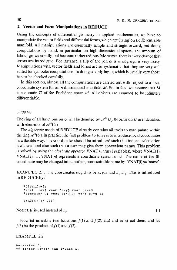
V = X I o x ~ X2 3 ~ + s i n (xlx2)-Ox 3 i 8x2
SYMBOLIC COMPUTATIONS IN APPLIED DIFFERENTIAL GEOMETRY
becomes in REDUCE:
57
*v :=xl*d-x2^ 3*dA2+s in(x l*x2)*d" 35
To determine the coefficients of V and printing them, you may type the following commands:
*array aa 3; dlm:=coeff(v,d,aa);
DIM := 3
*for i:=1:3 do write aa i:=aa i;
AA(1) := Xl 3
AA(2) := - X2 AA(3) := SIN(XI*X2)
[]
Note: Due to this approach, we can use the input and output facilities of REDUCE for vector fields. The ordinary operations with vector fields, addition and multi- plication with functions in d~ are therefore standard operations with poly- nomials in REDUCE.
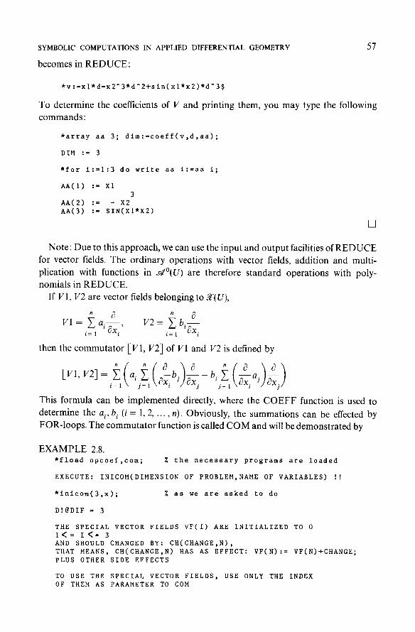
If V1, V2 are vector fields belonging to Y'(U),
V I = ~'~ e l i = ~"Y i ' V 2 = ~-'l b i c? x =
then the commutator [V1, V2] of V1 and V2 is defined by
:( [V1, V2] = a i b 2 - - b i aj i=1 j= j = l
This formula can be implemented directly, where the COEFF function is used to
determine the a i, bi ( i -- l, 2 . . . . . n). Obviously, the summations can be effected by FOR-loops. The commutator function is called COM and will be demonstrated by
EXAMPLE 2.8. *fload opcoef,com;
EXECUTE: IN
*inicom(3,x
D!@DIF = 3
THE SPECIAL I<= I<= 3 AND SHOULD CHANGED BY: CH(CHANGE,N), THAT MEANS, PLUS OTHER
TO USE THE OF THEM AS
ICOM(DIMENSlON OF PROBLEM,NAME OF VARIABLES)
); % as we are asked to do
% the necessary programs are loaded
!!
VECTOR FIELDS VF(1) ARE INITIALIZED TO 0
CH(CHANGE,N) HAS AS EFFECT: VF(N) := VF(N)+CHANGE; SIDE EFFECTS
SPECIAL VECTOR FIELDS, USE ONLY THE INDEX PARAMETER TO COM

58
THE LOCAL COORDINATES ARE XI,...,X3
INICOMEND
*vl:=x3*d$ v2:=xl*d^2-d^3$ ch(vl,l);
CHEND
Now two special vector fields are initialized.
*on test;
368 MS
P. K. H. GRAGERT ET AL.
ch(v2,2)$
By this switch, execution times are printed too, and differences in execution time can be observed.
*com(l,2);
2 D *X3 + D
30 MS
*com(vl,v2); % the same commutator again
2 D *X3 + D
47 MS
*com(l,xl*d-sin x2*d^2+x3*cos xl*d~3);
3 2 - D *X3 *SIN(XI) + D'X3*( - COS(X1) + i)
104 MS [ ]
I N N E R PRODUCT OF VECTOR FIELDS A N D FORMS
The inner product of vector fields and differential forms is a d~ mapping:
IP : a t (u ) x ~ m ( u ) --, d m- l (u )
where d - I(U) = 0 by definition.
It suffices to define the action of IP on basis elements BVF and BF(i), i.e., to define
I P ( • , dx , ) . \ a x ,
In our implementation in REDUCE this action can be described as follows:
0
SYMBOLIC COMPUTATIONS IN APPLIED DIFFERENTIAL GEOMETRY 59
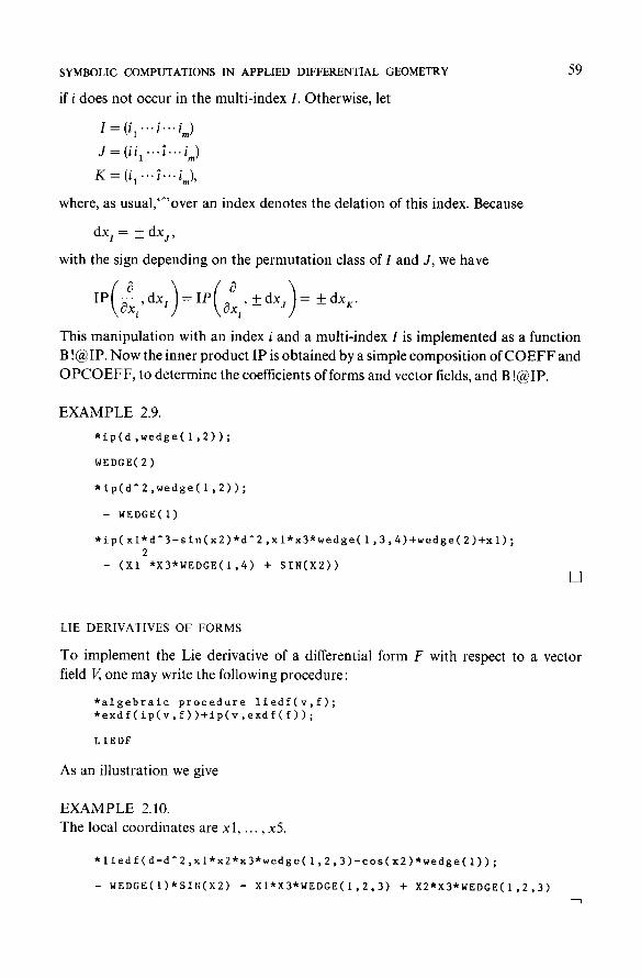
if i does not occur in the multi-index I. Otherwise, let
I = (i~ . . . i . . . im)
J -- (i i l . . . ~... i )
K = (i 1 " " 7 " " i r a ) ,
where, as usual, '~'over an index denotes the delation of this index. Because
dx i = _+ dx~,
with the sign depending on the permutation class of I and J, we have
This manipulation with an index i and a multi-index I is implemented as a function B !@IP. Now the inner product IP is obtained by a simple composit ion of C O E F F and
O P C O E F F , to determine the coefficients of forms and vector fields, and B !@IP.
EXAMPLE 2.9.
*ip(d,wedge(l~2));
WEDGE( 2 )
*ip(d ̂ 2,wedge(l,2));
- WEDGE(i)
*ip(xl*d^3-sin(x2)*d^2,xl*x3*wedge(l,3,4)+wedge(2)+xl) ; 2
(El *E3*WEDGE(I,4) + SIN(X2)) []
LIE DERIVATIVES OF FORMS
To implement the Lie derivative of a differential form F with respect to a vector field V, one may write the following procedure:
*algebraic procedure liedf(v,f); *exd f (ip(v, f))+ip(v,exdf (f)) ;
LIEDF
As an illustration we give
EXAMPLE 2.10. The local coordinates are xl , . . . , x5.
*liedf(d-d ̂ 2,xl*x2*x3*wedge(l,2,3)-cos(x2)*wedge(1));
- WEDGE(1)*SIN(X2) - XI*X3*WEDGE(I,2,3) + X2*X3*WEDGE(I,2,3)
60 P . K . H . GRAGERT ET AL.
Note: One may obtain a somewhat faster procedure, if the existing functions EXDF and IP are not used as above, but instead, a procedure for the Lie derivative
is constructed directly.
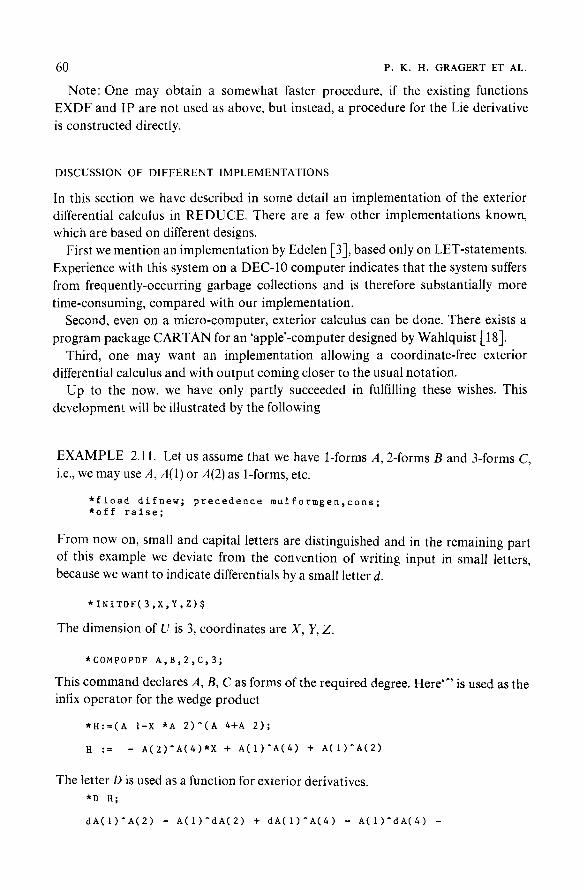
DISCUSSION OF DIFFERENT IMPLEMENTATIONS
In this section we have described in some detail an implementation of the exterior differential calculus in REDUCE. There are a few other implementations known, which are based on different designs.
First we mention an implementation by Edelen [3], based only on LET-statements.
Experience with this system on a DEC-10 computer indicates that the system suffers from frequently-occurring garbage collections and is therefore substantially more
time-consuming, compared with our implementation. Second, even on a micro-computer, exterior calculus can be done. There exists a
program package CARTAN for an 'apple'-computer designed by Wahlquist [18]. Third, one may want an implementation allowing a coordinate-free exterior
differential calculus and with output coming closer to the usual notation. Up to the now, we have only partly succeeded in fulfilling these wishes. This
development will be illustrated by the following
EXAMPLE 2.11. Let us assume that we have 1-forms A, 2-forms B and 3-forms C, i.e., we may use A, A(1) or A(2) as 1-forms, etc.
*fload difnew; precedence mulformgen,cons; *off raise;
From now on, small and capital letters are distinguished and in the remaining part of this example we deviate from the convention of writing input in small letters, because we want to indicate differentials by a small letter d.
INITDF( 3 ,X, u Z) $
The dimension of U is 3, coordinates are X, Y, Z.
* COMPOPDF A,B,2,C,3;
This command declares A, B, C as forms of the required degree. Here' ̂ ' is used as the infix operator for the wedge product
*H:=(A l-X *A 2)"(A 4+A 2);
H := - A(2)AA(4)*X + A(1)AA(4) + A(1)'A(2)
The letter D is used as a function for exterior derivatives. *D H;
dA(1)AA(2) A(1)^dA(2) + dA(1)^A(4) - A(1)^dA(4) -

SYMBOLIC COMPUTATIONS IN APPLIED DIFFERENTIAL GEOMETRY
dX*A(2)*A(4) - dA(2)~A(4)*X + A(2)*dA(4)*X
�9 H2 :=(B+Z~B I) ~(B+555*A) ;
H2 := B(1)^B*Z + 555*A^B(1)*Z + 555*A^B
�9 D H2;
555*dZ'A^B(1) + 555*dA'B(1)*Z - 555~A*dB(1)~Z + dZ'B(1)^B +
dB(1)^B*Z + dB^B(1)~Z + 555~dA~B + 555~dB^A []
Note: On account of its experimental state, the details of this package are not included in the Appendix. We hope to report on this in future work.
61
3. Infinitesimal Symmetries of Exterior Differential Systems.
As an application of the above-developed software, we treat infinitesimal symmetries of partial differential equations by means of differential geometric methods. Follow- ing Cartan, partial differential equations can be described geometrically by exterior differential systems [2, 7, 10].
We consider an exterior differential system I in a domain U of a n-dimensional manifold M, and suppose that I is generated by the finite set of forms
~(1), . . . , ct(m). (3.1)
By definition, infinitesimal symmetries are vector fields V such that
~ v I c I (3.2)
where Lf v denotes the Lie derivative by the vector field V[7, 10]. In physical literature, infinitesimal symmetries are also called isovectors.
Note: In the case that I is generated by k-forms fl(1), . . . , fl(r) and their exterior derivatives, it suffices to require (3.2) to hold for these k-forms fl(1) . . . . . fl(r) only, due to the fact that exterior derivative and Lie derivative commute
dS~ = ~ v d. (3.3)
The relation (3.2) is equivalent to
m
~ v ~ ( i ) - ~ y(i,j)/x ct(j)= 0 (3.4) j = l
with y(i,j) suitably-chosen differential forms.
If X(1) . . . . . X(n) are local coordinates in U and if we describe forms and fields locally in these coordinates
n
V = ~ v i c~ i= 1 ~X(i) (3.5)
~(i) = ~ A,,...ip(X)dX(il)/x ... A.dX(ip), i l . . . . . i p

62 P K. H. GRAGERT ET AL.
then (3.4) yields the conditions on V in order to be an infinitesimal symmetry This leads to an overdetermined system of partial differential equations for the functions
V i (i = 1 . . . . . n).
E X A M P L E 3.1. In this example we shall derive the first set of partial differential equations for the determination of the infinitesimal symmetries of Burgers' equation,
U r = Uxx + 2UU x.
The ideal I in R 4 = { (X(1), X(2), X(3), X(4))} -- {(X, T, U, Ux) ) is generated by
~(1) = - d T / x d U - U x d X / x d T
~(2) = - d T / x dU x - d X /x d U ~ 2 U U x d X /x d T
First we call the necessary programs and declare some algebraic operators.
*fload opcoef,diffor; operator x,v,alfa,aa,ver;
GIVE VALUES TO D!@DIF AND VNAT(1) I=3,...,DX@DIF (VNAT I=X, VNAT 2=T)
*in tools .red ,opl .red, Ip .red,bevat .red, lle. reds
IP EXECUTE: ARRAY A!@IP(MAXIMAL DIMENSION); LIEDF LE
*d!@dif:=4;
D@DIF := 4
*array a!@ip 4; for i:=1:4 do vnat i:=x i; *vec:=for i:=1:4 sum v(i,var)*d^i;
4 3 2 VEC := D *V(4,VAR) + D *V(3,VAR) + D *V(2,VAR) + D*V(I,VAR)
We introduce functions V(I, VAR), meaning functions dependent on the variables X(1) . . . . . X(4), generating the vector field VEC (V in (3.5))
*for all i,j let df(v(i,var),x j)=v(i,x j);
Due to the introduction of VAR in the functions V(I, VAR) (I = 1, 2, 3, 4) we are able to 'create' partial derivatives V(I,X(J)) by this LET-statement, although V(I, VAR) does not explicitly depend on X(1), . . . , X(4).
*alfa l:=-wedge(2,3)-x 4*wedge(l,2)$ *alfa 2:=-wedge(l,3)+2*x 3*x 4*wedge(l,2)-wedge(2,4)$ *la:=liedf(vec,alfa l)-aO*alfa l-al*alfa 2;
LA := WEDGE(3,4)*V(2,X(4)) + WEDGE(2,4)*(AI + V(I,X(4))*X(4) - V
(3,X(4))) + WEDGE(2,3)*(V(I,X(3))*X(4) V(3,X(3)) +

SYMBOLIC COMPUTATIONS IN APPLIED D~FERENTIALGOEMETRY
A0 - V(2,X(2))) - WEDGE(I,4)*X(4)*V(2,X(4)) +
WEDGE(I,3)*( - V(2,X(3))*X(4) + A! - V(2,X(1))) +
WEDGE(I,2)*( - V(I,X(1))*X(4) + V(3,X(1)) + AO*x(4)
2*AI*X(3)*X(4) - X(4)*V(2,X(2)) - V(4,VAR))
LA = 0 is just requirement (3.4) for ALFA(1).
Using O P C O E F F we calculate the coefficients WEDGE (3, 4) . . . . . which have to be zero, and print them.
*aant:=opcoeff(la,wedge,ce);
AANT := 5
*for I:~O:5 do write aa(l,i) :fficc(l,i);
63
AA(I,0) := V(2,X(4))
AA(I,I) :ffi - X(4)*V(2,X(4))
AA(I,2) :ffi A1 + V(I,X(4))*X(4) - V(3,X(4))
AA(I,3) := - V(2,X(3))*X(4) + A1 - V(2,X(1))
AA(I,4) :ffi - V(I,X(1))*X(4) + V(3,X(1)) + A0*X(4) - 2*AI*X(
3)*X(4) - X(4)*V(2,X(2)) - V(4,VAR)
AA(I,5) := V(I,X(3))*X(4) - V(3,X(3)) + A0 - V(2,X(2))
AA(1, J) are the coefficients of the basis-forms and we now eliminate A0, A1, by the use of OP L and retain theremainingequations.
*opl(aa(l,2),al)$ al:=al;
A1 :ffi - V(I,X(4))*X(4) + V(3,X(4))
*opl(aa(t,5),a0)$
*vet l:~aa(l,0)$ ver *ver 4:~aa(1,4)$ *for i:'-1:4 d o write
VER(1) :ffi V(2,X(4))
VER(2) :ffi - X(4)*V(2,X(4))
VER(3) :- - V(2,X(3))*X(4)
- V ( 2 , X ( 1 ) )
2 : f f i a a ( 1 , 1 ) $ v e r 3 : - a a ( 1 , 3 ) $
v e r l : f f i v e r i ;
- V ( 1 , X ( 4 ) ) * X ( 4 ) + V ( 3 , X ( 4 ) )
V E R ( 4 ) := - v ( l , x ( 1 ) ) * x ( 4 ) + v ( 3 , x ( 1 ) ) - v ( t , x ( 3 ) ) * x ( 4 )
2 V(3,X(3))*X(4) + 2*V(I,X(4))*X(3)*X(4)
- 2*V(3,X(4))*X(3)*X(4) - V(4,VAR)
2 +
[]
of the basis-forms,

64 P . K . H . GRAGERT ET AL.
The process of computing the whole system of partial differential equations for the functions V i (i = 1 . . . . . n) runs along similar lines, as in Example 3.1, and is done automatically by the procedure INFSYM(VOR, N1, N) in the appendix, where VOR is the name of the differential forms generating I (3.1), N1 is the number of differential forms, and N is the dimension of R'.
Once the system of partial differential equations has been derived, we have to solve it for the functions V(I, VAR). In general, it is not possible to solve them auto- matically; but it turns out that in the most interesting cases, e.g., nonlinear evolution equations such as Korteweg-de Vries and Burgers', and field equations such as Maxwell and Dirac equations, solutions are of polynomial type and, therefore, we are able to compute them semi-automatically [9, 12].
The process of automization of solving these overdetermined systems is still in progress, and we shall discuss two frequently occurring cases.
(A) Usually there are equations in this system of type
VER(J) := V(I, X(K))
for some I, K; from which we derive
V(I, VAR) is independent of X(K).
Procedure ONE( )searches for such equations and assigns zero to the function V(I, X(K)).
(B) In most cases, the system of partial differential equations is linear in V(I, X(J)), V(K, VAR) (we shall denote these by V(I, ,)) with coefficients which are polynomials in some of the variables X(1) . . . . . X(N).
If an equation contains only terms V(I, *) independent of X(I~), ..., X(Ir), (results, which can be obtained by procedure ONE( ) ) and if the coefficients are polynomials in X(I1 ) . . . . . X(Ir) , we consider this equation as a polynomial in X(I 1) . . . . . X(I) and split up this equation into a set of smaller equations, due to the fact that the coefficients of this polynomial have to be zero.
This analysis is carried out by SPLITI(K), which searches for a polynomial struc- ture in VER(K), or SPLITS(), which deals with the whole system.
SCHEM( ) is a procedure that creates lists !@A(L) of numbers representing partial derivatives which are zero. !@A(2) = (1, 4) means V(2, X(1)) = 0; V(2, X(4))= 0 FIG( ) prints a diagram of partial derivatives being zero.
EXAMPLE 3.2. First we load some necessary programs.
*fload opcoef; *in tools.red,opl.red,split.red$
TELl := 0
*in mlie$ EXECUTE : ARRAY !@A(DI@DIF)$
EXECUTE : ARRAY AI@FIG(D!@DIF)$

SYMBOLIC C O M P U T A T I O N S IN A P P L I E D DIFFERENTIAL GEOMETRY 6 5
We read a file which contains a system of five equations (TOTAAL = 4), while the number of variables is 7 (D !@DIF = 7); so V(I, VAR) is dependent on X(1), . . . , X(7).
*in tests
VER(0) := V(I,X(2)) + X(3)*V(I,X(4))
VER(1) := V(I,X(4))
VER(2) := V(I,X(2))*X(1) + 3*X(4)*V(I,X(3))
2 VER(3) := X(2) *V(I,X(7)) + X(3)*V(l,X(6))
VER(4) := X(4)*V(2,X(5)) + V(I,X(6))
TOTAAL := 4
D@DIF := 7
*array l@a d!@dif,a!@fig d!@dif;
These aretheini t ia t ionsrequired bythesystem:
*one()$
V(i,X(4))
0
V(I,X(2))
0
v(1,x(3))
o
2 V E R ( 3 ) := X ( 2 ) * V ( 1 , X ( 7 ) ) + X ( 3 ) * V ( 1 , X ( 6 ) )
VER(4) := X(4)*V(2,X(5)) + V(I,X(6))
ONE sets V(1, X(4)), V(1, X(2)), V(1, X(3)) equal to zero and prints the remaining set of nontrivial equations.
* f i g ( ) , VlJ I 2 3 4 5 6 7
1 * * * * * * * 2 0 * * * * * * 3 0 * * * * * * 4 0 * * * * * *
5 * * * * * * *
6 * * * * * * * 7 * * * * * * *
From FIG we see that V(1, X(2)) = V(1, X(3)) = V(1, X(4)) = 0.
* z e r o d e l e t e ( ' v e r ) $

66 P . K . H . GRAGERT ET AL.
This is a procedure that deletes trivial equations, i.e.,
VER(I) := 0
from the system.
*splits()$
O-TH EQUATION : YES!I(2 3 4) I-TH EQUATION : NO! !
TOTAAL : = 2
From the message of the procedure SPLITS we see that equation 0 (i.e., VER(3) above, because ZERODELETE has renumbered the equations) is a polynomial in X(2), X(3) and X(4). The coefficients of this polynomial, which have to be zero, generate a new and larger set of equations.
*for i:=0:totaal do write v e t i:=ver i;
VER(0) := X(4)*V(2,X(5)) + V(I,X(6))
VER(1) := V(I,X(6))
VER(2) := V(I,X(7))
VER(1),VER(2) are Just the coefficients of VER(3) above.
*one()$
v(i,x(6))
0
v(1,x(7))
0
V(2,X(5))
0
Now all equations are trivial, so there is no remaining set to be printed.
*fig()$
VIJ I 2 3 4 5 6 7
1 * * * * * * *
2 O * * * * * * 3 O * * * * * * 4 0 * * * * * *
5 * 0 * * * * * 6 0 * * * * * * 7 0 * * * * * * []
We applied this to the computation of the infinitesimal symmetries of the Lin- Reisner-Tsien equation (unsteady transonic gas motion)
UxUxx - 2ux, + u y = O.

SYMBOLIC COMPUTATIONS IN APPLIED DIFFERENTIAL GEOMETRY 67
The ideal I in R 12 -- {(x(1) .... ,x(12))} -- {(x, t, y, u, u x, u t, uy, u x, Uxt, u y, u . , u,y)} is generated by the 1-forms
ALFA(1):=WEDGE(4)-x(5) *WEDGE(1)-x(6) *WEDGE(2)-x(7) *WEDGE(3) ALFA(2):=WEDGE(5)-x(8) *WEDGE(1)-x(9) *WEDGE(2)-x(10) *WEDGE(3) ALFA(3) :=WEDGE(6)-x(9) *WEDGE(1)-x(II)*WEDGE(2)-x(12) *WEDGE(3) ALFA(4):=WEDGE(7)-x(IO)*NEDGE(1)-x(12)*WEDGE(2)-PSI(1)*WEDGE(3) PSI(1):= 2"X(9)+ X(5)*X(8)
and their exterior derivatives.
Due to (3.4) we shall omit EXDF(ALFA(I))(I: = 1:4). We calculated the following infinitesimal generators of the group of symmetries
V x = V(1, VAR) = xF'(t) + y2F"(t) + yG'(t) + H(t) + 2Ax.
V t = V(2, VAR) = 3V(t)
V" = V(3, VAR) = 2yV'(t) + Gtt) + A y (3.6)
V" = V(4, VAR) = - uF'(t) + x2F"(t) + 2xyZF ' '(t) +
+ 1/3y4F""(t) + 2xyG"(t) + 2/3 y3G"'(t) +
+ 2xH'(t) + 2y2H"(t) + ya( t ) + z(t) + 4Au
where F, G, H, a, z are arbitrary functions of t, A is constant, and denotes differentia- tion. For simplicity, we omit the functions V"x,.. . , which can be derived from (3.6) by prolongation. This result is in agreement with that of Anderson and Ibragimov [1, p. 73], apart from the generator arising from A.
4. Conclusions
In principal, anything which can be achieved by symbolic calculations can be achieved by hand and vice versa. By using the computer, however much valuable time can often be saved.
We invite the reader to do symbolic calculations in REDUCE himself and to experience with the material presented in this paper. We are aware that various improvements can be made, and so further suggestions will be most welcome.
If a reader is interested in the functions in the Appendix, it may be of help to get a
copy on magnetic tape. This can be arranged by sending a blank tape to one of the authors.
Appendix ~OPCOEF.R~D tO-FEB-alL SCALAR !0RESTOPeOEFFS LISP OPERATOR OPCOEFF$
LISP PROCEDURE GETFIRSTOP(FORM,L,OP); %C GETFIRSTOP.i; IF ATOM FORM THEN L %C ii;
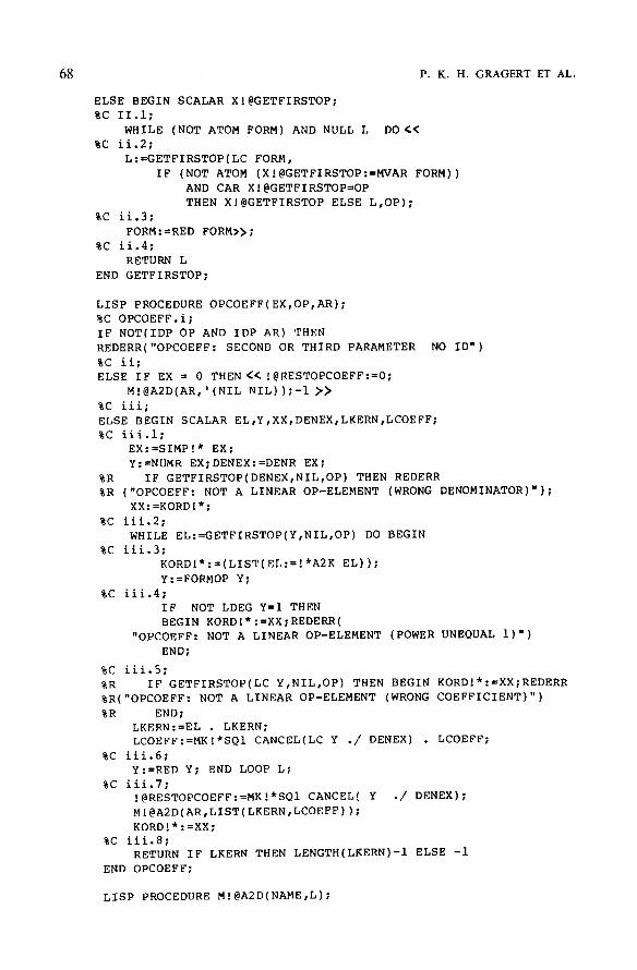
68 P. K. H. GRAGERT ET AL.
ELSE BEGIN SCALAR X!@GETFIRSTOP; %C II.l;
WHILE (NOT ATOM FORM) AND NULL L DO << %C ii.2;
L:=GETFIRSTOP(LC FORM, IF (NOT ATOM (XI@GETFIRSTOP:=MVAR FORM))
AND CAR X!@GETFIRSTOP=OP THEN Xl@GETFIRSTOP ELSE L,OP);
%C ii.3; FORM:=RED FORM,>;
%C ii.4; RETURN L
END GETFIRSTOP;
LISP PROCEDURE OPCOEFF(EX,OP,AR); %C OPCOEFF.i; IF NOT(IDP OP AND IDP AR) THEN REDERR("OPCOEFF: SECOND OR THIRD PARAMETER NO ID")
%C ii; ELSE IF EX = 0 THEN << !@RESTOPCOEFF:=0;
Mi@A2D(AR,'(NIL NIL));-1 >>
%C iii; ELSE BEGIN SCALAR EL,Y,XX,DENEX,LKERN,LCOEFF; %C ill.l;
EX:=SIMP!* EX; Y:=NUMR EX;DENEX:=DENR EX;
%R IF GETFIRSTOP(DENEX,NIL,OP) THEN REDERR %R ("OPCOEFF: NOT A LINEAR OP-ELEMENT (WRONG DENOMINATOR)W);
XX:=KORD!*; %C iii.2;
WHILE EL:=GETFIRSTOP(Y,NIL,OP) DO BEGIN %C iii.3;
KORDI*:=(LIST(EL:=!*A2K EL));
Y:=FORMOP Y; %C iii.4;
IF NOT LDEG Y=I THEN BEGIN KORD!*:=XX;REDERR(
"OPCOEFF: NOT A LINEAR OP-ELEMENT (POWER UNEQUAL i) w)
END;
%C iii.5; %R IF GETFIRSTOP(LC Y,NIL,OP) THEN BEGIN KORDI*:=XX;REDERR %R("OPCOEFF: NOT A LINEAR OP-ELEMENT (WRONG COEFFICIENT)")
%R END; LKERN:=EL . LKERN; LCOEFF:=MK!*SQI CANCEL(LC Y ./ DENEX) . LCOEFF;
%C iii.6; Y:=RED Y; END LOOP L;
%C iii.7; !@RESTOPCOEFF:=MK!*SQI CANCEL( Y ./ DENEX); MI@A2D(AR,LIST(LKERN,LCOEFF));
KORDI*:=XX; %C iii.8;
RETURN IF LKERN THEN LENGTH(LKERN)-I ELSE -i
END OPCOEFF;
LISP PROCEDURE MI@A2D(NAME,L);
SYMBOLIC COMPUTATIONS IN APPLIED DIFFERENTIAL GEOMETRY 69
%C [email protected]; BEGIN IF NULL GET(NAME,'I@OPELEMENT) THEN %C ii;
(<FLAG(LIST(NAME),'OPFN); PUTD(NAME,'EXPR,LIST('LAMBDA,'(I0 Ii), LIST('NTH, LIST('NTH,LIST('GET, MKQUOTE NAME, MKQUOTE '!@OPELEMENT), '(ADD1 I0)),'(ADDI If))) )>>;
%C iii; PUT(NAME,'!@OPELEMENT,L);
END MI@A2D; %DIFFOR.RED 6-APR-1981; SCALAR !@RESTOPCOEFF,D!@DIF,I@UIT; OPERATOR VNAT,UIT; LISP OPERATOR EXDF,MULFORM,NORMDIF$
%INITIALIZATIONS; WRITE( "GIVE VALUES TO DI@DIF AND VNAT(I) I=3,...,D!@DIF (VNAT I=X, VNAT 2= T)")$ FACTOR UIT$OFF ALLFAC$ VNAT(1)d:=X;VNAT(2):=T; LISP !@UIT:=WEDGE$
LISP PROCEDURE I@REPEATSONCE X; %C [email protected]; IF NULL X THEN NIL %C ii; ELSE IF CAR X MEMBER CDR X THEN T %C iii; ELSE !@REPEATSONCE CDR X;
LISP PROCEDURE MERGESTRICT(LA,LB); %C MERGESTRICT.i; BEGIN SCALAR LALB,RES; %C ii; RETURN IF !@REPEATSONCE (LALB:=APPEND(LA,LB)) THEN '(0) %C iii; ELSE IF PERMP(LALB,RES:=REVERSIP ORDN LALB) THEN 1 . RES %C iv; ELSE (-i) . RES END MERGESTRICT;
LISP PROCEDURE MULFORM(A,B); %C MULFORM.i; BEGIN INTEGER F,DI,D2;
SCALAR H3,AMULII,RES,AREST,BREST,ELA,ELB,LI; %C ii;
DI:=OPCOEFF(A,!@UIT,'I@AMUL);AREST:=I@RESTOPCOEFF; D2:=OPCOEFF(B,!@UIT,'!@BMUL);BREST:=I@RESTOPCOEFF;
%C iii; %C ill.l;
RES:=AEVAL LIST('PLUS, LIST('TIMES,AREST,B), LIST('TIMES,BREST,AEVAL LIST('DIFFERENCE,A,AREST)));
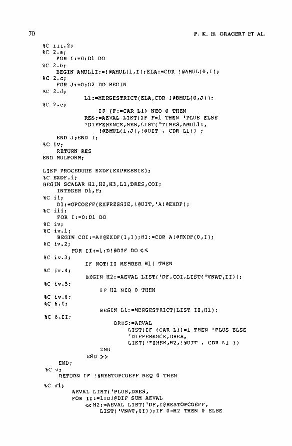
70 P. K. H. GRAGERT ET AL.
%C 111.2; %C 2.a;
FOR I:=0:DI DO %C 2.b;
BEGIN AMULII:=!@AMUL(I,I);ELA:=CDR !@AMUL(0,I); %C 2.c;
FOR J:=0:D2 DO BEGIN
%C 2.d; LI:=MERGESTRICT(ELA,CDR !@BMUL(0,J));
%C 2.e; IF (F:=CAR LI) NEQ 0 THEN
RES:=AEVAL LIST(IF F=I THEN 'PLUS ELSE 'DIFFERENCE,RES,LIST('TIMES,AMULII,
!@BMUL(I,J),!@UIT . CDR LI)) ; END J;END I;
%C iv; RETURN RES
END MULFORM;
LISP PROCEDURE EXDF(EXPRESSIE); %C EXDF.i; BEGIN SCALAR HI,H2,H3,LI,DRES,COI;
INTEGER DI,F;
%C ii; DI:=OPCOEFF(EXPRESSIE, !@UIT,'A!SEXDF);
%C iii; FOR I:=0:DI DO
%C iv; %C iv.l;
BEGIN COI:=A!@EXDF(I,I);HI:=CDR A!@EXDF(0,I); %C iv.2;
FOR II:=I:D!@DIF DO << %C iv.3;
IF NOT(II MEMBER HI) THEN %C iv.4;
%C iv.5;
%C iv.6; %C 6.I;
%C 6.II;
BEGIN H2:=AEVAL LIST('DF,COI,LIST('VNAT,II));
IF H2 NEQ 0 THEN
BEGIN LI:=MERGESTRICT(LIST II,HI);
DRES:=AEVAL LIST(IF (CAR LI)=I THEN 'PLUS ELSE 'DIFFERENCE,DRES, LIST('TIMES,H2,!@UIT . CDR L1 ))
END
END >> END;
%C v; RETURN IF !@RESTOPCOEFF NEQ 0 THEN
%C vi; AEVAL LIST( 'PLUS,DRES, FOR II:=I:D!@DIF SUM AEVAL
<<H2:=AEVAL LIST( 'DF,!@RESTOPCOEFF, LIST('VNAT,II) );IF 0=H2 THEN 0 ELSE

SYMBOLIC COMPUTATIONS IN APPLIED DIFFERENTIAL GEOMETRY
LIST('TIMES,H2,LIST(!@UIT,II))~>)
%C vii;
ELSE DRES END EXDF;
LISP OPERATOR NORMDIF; LISP PROCEDURE NORMDIF(X); %C NORMDIF.i; BEGIN INTEGER D;SCALAR L;
%C ii; D:=OPCOEFF(X,!@UIT,'OP!@NORMDIF);
%C iii; RETURN AEVAL LIST('PLUS,!@RESTOPCOEFF,
FOR I:=0:D SUM IF CAR(L:=MERGESTRICT(CDR OPI@NORMDIF(0,I),NIL)) = 0 THEN 0 ELSE LIST('TIMES,CAR L,OP!@NORMDIF(I,I), I@UIT . CDR L))
END NORMDIF; %COM.RED 7-JUL-81;
ARRAY AI@COM(I,I); SCALAR DI@DIF,D!@DIFPI,D!@DIFP2,I@VECVAR; OPERATOR VNAT,Di@COM,VF; LISP OPERATOR NIEUWCOEFF,FILVNAT$
WRITE("EXECUTE: INICOM(DIMENSION OF PROBLEM,", "NAME OF VARIABLES) 
72 P. K. H. GRAGERT ET AL.
D!@DIF:=N;DI@DIFPI:=N+I;DI@DIFP2:=N+2;
FILVNAT(N,NAME);ARRAY AI@COM(N+2,N); WRITE(
"THE LOCAL COORDINATES ARE ",VNAT(1),",...,",VNAT(N)); RETURN INICOMEND
END INICOM$
LISP PROCEDURE NIEUWCOEFF(A,XX,NAM,I)$ COEFF(A,XX,LIST(NAM,I,'TIMES))$
ALGEBRAIC PROCEDURE COM(I,J); %C COM.i; BEGIN INTEGER DI,DJ; %C ii;
IF NOT(NUMBERP I AND I 0 AND I =DI@DIF)
%C iii; THEN (<DI:=NIEUWCOEFF(I,!@VECVAR,A!@COM,D!@DIFPI);
I:=D!@DIFPI >>
%C iv; ELSE DI:=D!@COM(I);
%C v; IF NOT(NUMBERP J AND J)0 AND J<=D!@DIF)
%C vi; THEN'(DJ:=NIEUWCOEFF(J,I@VECVAR,AI@COM,D!@DIFP2);
J:=DI@DIFP2 ~
%C vii; ELSE DJ:=DI@COM(J);
%C viii; RETURN FOR II:=I:DI SUM IF A!@COM(I,II) NEQ 0 THEN FOR JJ:=I:DJ SUM IF A!@COM(J,JJ)NEQ 0 THEN (AI@COM(I,II)*I@VECVARAJJ*DF(A!@COM(J,JJ),VNAT(II)) - A!@COM(J,JJ)*!@VECVAR^II*DF(AI@COM(I,II),VNAT(JJ)))
ELSE 0 ELSE 0
END COM$
%IP.RED 25-MAR-81;
ARRAY AI@IP(0); SCALAR !@UIT,I@VECVAR$ LISP OPERATOR REDERR,BI@IP$ OPERATOR UIT$ LISP [@VECVAR:='D$ LISP I@UIT:='WEDGE$
LISP PROCEDURE B!@IP(IND,BUIT);
%C [email protected]; BEGIN SCALAR H,FAC; %C ii;
RETURN IF IND MEMBER (H:=CDR BUIT) THEN %C iii;
IF LENGTH H=I THEN 1 %C iv;
ELSE<(FAC:=I; WHILE (IND NEQ CAR H) DO<(FAC:=-FAC;H:=CDR H>);
%C v;- AEVAL LIST('TIMES,FAC,DELETE(IND,BUIT))>)
%C vi; ELSE 0
END B!@IP;

SYMBOLIC COMPUTATIONS IN APPLIED DIFFERENTIAL GEOMETRY
PROCEDURE IP(X,ALFA); %C IP.i; BEGIN SCALAR CO,IND;INTEGER DX,DA; %C ii;
DX:=COEFF(X, !@VECVAR,A!@IP); %C iii;
IF Ai@IP(0) NEQ 0 THEN REDERR("IP: NO GOOD VECTORFIELD GIVEN");
%C iv; DA:=OPCOEFF(
%R NORMDIF ALFA,!@UIT,UITi@IP);
%C v; RETURN FOR I:=I:DX SUM
%C vi; %C vi.l;
IF (CO:=AI@IP(I)) = 0 THEN 0
%C vi.2; ELSE << FOR J:=0:DA SUM
%C vi.3; (BZ@IP(I,UITI@IP(0,J))*CO*UIT!@IP(I,J) )7>
END IP;
CLEAR A!@IP; WRITE("EXECUTE: ARRAY Ai@IP(MAXIMAL DIMENSION);"); %OPL.RED 15-APR-81$ OFF ECHO$ ARRAY A!@OPL(1)$ LISP OPERATOR OPL,D!@MAX$
LISP PROCEDURE OPL(WAT,WAARNA)$ IF D!@MAX(WAT,WAARNA)=I THEN BEGIN COEFF(WAT,WAARNA,'A!@OPL)$
RETURN SETK(WAARNA,AEVAL LIST('MINUS ,LIST('QUOTIENT,GETEL LIST('A!@OPL,0), GETEL LIST('A!@OPL,I))))END
ELSE WRITE(WAARNA," NOT A KERNEL OR EXPRESSION NOT LINEAR WITH RESPECT TO ",WAARNA);
LISP PROCEDURE D!@MAX(EPR,VARI)$ MAXDEGREE(NUMR SIMP EPR,VARI)$
LISP PROCEDURE MAXDEGREE(FORM,VARI)$ IF DOMAINP FORM THEN 0 ELSE IF MVAR FORM = VARI THEN LDEG FORM ELSE MAX2(MAXDEGREE(LC FORM,VARI),MAXDEGREE(RED FORM,VARI))$ ON ECHO$
SCALAR TOTAAL,DI@DIF$ LISP OPERATOR CLEARKVALUE,LE; LISP PROCEDURE CLEARKVALUE(OP); <<REMPROP(OP,'KVALUE);0>>;
OPERATOR V,CO,B,LA,VER,OI@INF; PROCEDURE INFSYM(VOR,NI,N); BEGIN INTEGER M,MI, JJ,I,J,K;
ARRAY RA NI; FOR I:=I:NI DO B I:=NORMDIF(VOR I);
73

74
END;
P. K. H. GRAGERT ET AL.
M:=I;MI:=0; VEC:=(FOR I:=I:N SUM V(I,VAR)*DAI); FOR ALL X,II LET DF(V(II,VAR),X)=V(II,X); FOR JJ:=I:NI DO BEGIN AA:=!@BEVATOP(B(JJ),UIT);
RA(JJ):=LE AA; END; FOR I:=I:NI DO BEGIN
LA I:=LIEDF(VEC,B I)-(FOR J:=I:NI SUM MULFORM(GEFORM(J,RA I-RA J,N),B J));
AANT:=OPCOEFF(LA I,UIT,C); �9 OR K:=0:AANT DO bEGIN LII@INF:=OPCOEFF(C(I,K),CO,OI@INF);
S!@INF:=0; WHILE S!@INF LI!@INF+I DO IF (O!@INF(I,S!@INF)^2)=I THEN BEGIN OPL(C(I,K),OI@INF(0,SI@INF));
S!@INF:=LI!@INF+I; END ELSE S!@INF:=S!@INF+I;
END; FOR K:=0:AANT DO BEGIN L:=!@BEVATOP(C(I,K),CO);
IF L NEQ 0 THEN BEGIN WRITE "YOU ARE CREATING DENOMINATORS!!";
OPL(C(I,K),L) END
ELSE IF C(I,K) NEQ 0 THEN BEGIN VER M:=C(I,K); VER M:=VER M*D~ VER M; M:=M+I;
END; END; TOTAAL:=M-I;%ONETERMSOL(VER,TOTAAL); WRITE "THERE EXIST ",M-I-M1," EQUATIONS FOR THE ",I,"-TH MI:=M-I;CLEARKVALUE(CO);
END; VER 0:=0; FOR JJJ:=0:M-I DO WRITE VER JJJ:=VER JJJ; RETURN M-l;
PROCEDURE GEFORM(NR,J,N); IF J=0 THEN CO(NR,J) ELSE IF J=l THEN (FOR I:=I:N SUM CO(NR,J,I)*UIT I) ELSE IF J=2 THEN (FOR I:=I:N SUM (FOR K:=I+I:N SUM CO(NR,J,I,K)*UIT(I,K))) ELSE IF J=3 THEN (FOR I:=I:N SUM (FOR K:=I+I:N SUM (FOR L:=K+I:N SUM CO(NR,J,I,K,L)*UIT(I,K,L)))) ELSE 0
PROCEDURE PSP(N,M,K)$ FOR I:=M:K DO IF N I NEQ 0 THEN WRITE N I:=N IS
PROCEDURE ONETERMSOL(NAME,AANT)$ BEGIN M:=0$
FOR I:=0:AANT DO IF VER I NEQ 0 THEN IF OPCOEFF(VER I,V,I@CC)=0
AND I@RESTOPCOEFF=0 THEN BEGIN WRITE !@CC(0,0)$
M:=M+I$ !@B:=OPL(VER I,!@CC(0,0) WRITE !@B$
ENDS

SYMBOLIC COMPUTATIONS IN APPLIED DIFFERENTIAL GEOMETRY 75
IF M 0 THEN ONETERMSOL(NAME,AANT)$ ENDS
PROCEDURE ONE()$ BEGIN ONETERMSOL(VER,TOTAAL)$
PSP(VER,0,TOTAAL)$ ENDS PROCEDURE PS()$ PSP(VER,0,TOTAAL)$ PROCEDURE LPO(AANTI,AANT2)S BEGIN OPL(VER AANTI,V(AANT2,VAR))$
VER AANTI:=0$ ENDS
ARRAY I@A(0)$ LISP OPERATOR SCHEM,LX,LYSTX,TEST,TESTI$ LISP PROCEDURE LYSTX(L)$ BEGIN LX:=NIL$
WHILE L DO BEGIN LX:=LIST('X,CAR L).LX$ L:=CDR L
ENDS RETURN LX$
END LYSTX$
LISP PROCEDURE SCHEM()$ BEGIN FOR J:=I:DI@DIF DO !@A(J):=NIL$
FOR I:=I:D!@DIF DO FOR K:=I:DI@DIF DO IF REVAL LIST('V,I,LIST('X,K)) EQ 0 THEN !@A(K):=I.!@A(K)$
ENDS
ARRAY AI@FIG(0)$ LISP OPERATOR FIGS LISP PROCEDURE FIG()$ BEGIN SCALAR H$
H:=NIL$ SCHEM()$ FOR I:=DI@DIF STEP -i UNTIL 1 DO IF I i0 THEN H:='! .'l .I.H
ELSE H:='! .APPEND(EXPLODEC I,H)S H:='V.'I.'J.H$ SETEL('(A!@FIG 0),H)$ FOR J:=I:D!@DIF DO BEGIN H:=NIL$
FOR I:=D!@DIF STEP -i UNTIL 1 DO IF I MEMBER !@A(J) THEN H:='! .'! .'O.H
ELSE H:='! .'! '!*.HS IF J i0 THEN H:='! .'! .J.H
ELSE H:='! .APPEND(EXPLODEC J,H)$ SETEL(LIST('Ai@FIG,J),H)$
ENDS FOR J:=0:D!@DIF DO (<MAPCAR(GETEL LIST('AI@FIG,J),FUNCTION PRINC)$
TERPRI() >> END FIG $ WRITE "EXECUTE : ARRAY !@A(DI@DIF)$"S WRITE "EXECUTE : ARRAY AI@FIG(DI@DIF)$"$ ARRAY !@B 05
LISP OPERATOR SPLITS,SPLIT1;
LISP PROCEDURE SPLITS()$ BEGIN SCALAR RY,RYTJE,RES,TEL$
RY:=NIL$TEL:=0$

76
FOR II:=I:DI@DIF DO RY:=II.RY$ SCHEM()$ FOR JJ:=0:TOTAAL DO BEGIN RYTJE:=NIL$
P. K. H. G R A G E R T ET AL.
LB:=OPCOEFF(REVAL LIST('VER,JJ),'V,'!@CO)$ FOR EACH EL IN RY DO BEGIN RES:=NIL$
FOR KK:=0:LB DO IF CADR !@CO(0,KK) MEMBER !@A(EL) THEN NIL ELSE BEGIN KK:=LB+I$
RES:=T$ ENDS
IF RES THEN NIL ELSE RYTJE:=EL.RYTJE$
ENDS IF RYTJE=NIL THEN
BEGIN SETK(LIST('VER,TEL),REVAL LIST('VER,JJ))$ TEL:=TEL+I$ WRITE JJ,"-TH EQUATION : NO!!"$
END ELSE BEGIN MLIETAB(REVAL LIST('VER,JJ),LYSTX RYTJE)$
SETK(LIST('VER,JJ),0)$ WRITE JJ, "-TH EQUATION :",RYTJE$
ENDS ENDS FOR LL:=TEL:TEL+TELI-I DO SETK(LIST('VER,LL),REVAL LIST('PETER,LL-TEL+I))$ TOTAAL:=TEL+TELI-I$ CLEARKVALUE('PETER)$ TELI:=0$ WRITE "TOTAAL:=",TOTAAL$
END SPLITS $
LISP OPERATOR ZERODELETE; SCALAR LI@ZERODELETE; LISP PROCEDURE ZERODELETE NAME;BEGIN SCALAR LI,L2,TEL;
TEL:=0;LI@ZERODELETE:=NIL; FOR EACH XX IN GET(NAME,'KVALUE) DO IF REVAL(L2:=CADR XX)=0 THEN L!@ZERODELETE:=(CAR XX . '(0)) �9 LI@ZERODELETE ELSE LI:=(LIST(NAME,TEL:=TEL+I). LIST L2 ).LI; IF L1 THEN PUT(NAME,'KVALUE,REVERSIP LI) ELSE RETURN TEL
END;
LISP PROCEDURE SPLITI(JJ); BEGIN SCALAR RY,RYTJE,RES;
RY:=RYTJE:=NIL; FOR II:=I~DI@DIF DO RY:=II.RY; SCHEM(); LB:=OPCOEFF(REVAL LIST('VER,JJ),'V,'!@CO); FOR EACH EL IN RY DO BEGIN RES:=NIL;
FOR KK:=0:LB DO IF CADR !@CO(0,KK) MEMBER !@A(EL) THEN NIL ELSE BEGIN KK:=LB+I;
RES:=T; END;
IF RES THEN NIL ELSE RYTJE:=EL.RYTJE;
END;

SYMBOLIC COMPUTATIONS IN APPLIED DIFFERENTIAL GEOMETRY
IF RYTJE=NIL THEN BEGIN WRITE JJ,"-TH
RETURN 0 END
EQUATION : NOI!M;
ELSE BEGIN MLIETAB(REVAL LIST('VER,JJ),LYSTX RYTJE); SETK(LIST('VER,JJ),0); WRITE JJ,"-TH EQUATION :",RYTJE;
END; FOR LL:=TOTAAL+I:TOTAAL+TELI DO SETK(LIST( 'VER,LL),REVAL LIST( 'PETER,LL-TOTAAL); TOTAAL:=TOTAAL+TELI; CLEARKVALUE('PETER); TELl:=0; WRITE "TOTAAL:= ",TOTAAL;
END SPLITI;
77
References 1. Anderson, R. L. and Ibragimov, N. H. : Lie-Bi~cklund Transformations in Applications, SIAM Studies
in Applied Mathematics, Philadelphia, 1979. 2. Cartan, E. : Les systbmes difJ~rentiels et leurs applications g6om6triques, Hermann, Paris, 1945. 3. Edelen, D. G. B. : Isovector Methods for Equations of Balance, Sijthoffand Noordhoff, Alphen a/d Rijn,
The Netherlands, 1981. 4. Wahlquist, H. D. and Estabrook, F. B.: J. Math Phys. 16 (1975), 1-7. 5. Estabrook, F. B. and Wahlquist, H. D.: J. Math Phys. 17 (1976), 1293-1297. 6. Frick, I. : SHEEP's Users' Manual, University of Stockholm, 1977. 7. Estabrook, F. B. : 'Differential geometry as a tool for applied mathematicians, in R. Martini (ed.),
Geometric Approaches to DifJerential Equations (Lecture Notes in Mathematics, Vol. 810), Springer- Verlag, Heidelberg, New York, 1979.
8. Gragert, P. K. H. : 'Symbolic computations in prolongation theory', PhD thesis, Twente University of Technology, 1981.
9. Gragert, P. K. H. and Kersten, P. H. M.: 'Implementation of differential geometric objects and functions with an application to extended Maxwell equations', in J. Calmet (ed.), Proceedings Eurocam 1982 (Lecture Notes in Computer Science, Vol. 144), Springer-Verlag, Heidelberg, New York, 1982, pp. 181 187.
10. Harrison, B. K. and Estabrook, F. B.: J. Math. Phys. 12 (1971), 653-666. I 1. Hearn, A. C. : Reduce 2 Users" Manual, 2nd edition, University of Utah, 1973. 12. Kersten, P. H. M. : 'Infinitesimal symmetries and conserved currents for nonlinear Dirac equations',
to appear in J. Math. Phys. 13. Lewis, V. E. (ed.): MA CS YMA Users" Conference Proceedings, 1979, Washington D.C., MIT Labora-
tory of Computer Science, Cambridge, Mass., 1979. 14. McCarthy, J. et al. : LIPS 1.5 Programmers" Manual, MIT Press, Cambridge, Mass., 1962. 15. Molino, P. : 'Exterior differential systems and partial differential equations', Notes of invited lectures
at the University of Amsterdam, 1982. 16. REDUCE Newsletters, 1 (1978), 2 (1978), 3 (1978), 4 (1978), 5 (1979), 6 (1979), 7 (1979), Symbolic
Computation Group, University of Utah. 17. Risch, R. H.: Trans. Am. Math. Soc. 139 (1969), 167 189. 18. Wahlquist, H. D. : 'Exterior calculus on an Apple : the program "~CARTAN", preprint, 1981.
Related Documents