Symbolic AI for XAI: Evaluating LFIT Inductive Programming ...

Symbolic AI for XAI: Evaluating LFIT Inductive Programming

for Fair and Explainable Automatic Recruitment

Alfonso Ortega, Julian Fierrez, Aythami Morales, Zilong Wang

School of Engineering, Universidad Autonoma de Madrid

{alfonso.ortega,julian.fierrez,aythami.morales}@uam.es, [email protected]

Tony Ribeiro

Laboratoire des Sciences du Numerique de Nantes National Institute of Informatics Japan

tony [email protected]

Abstract

Machine learning methods are growing in relevance for

biometrics and personal information processing in domains

such as forensics, e-health, recruitment, and e-learning. In

these domains, white-box (human-readable) explanations of

systems built on machine learning methods can become cru-

cial. Inductive Logic Programming (ILP) is a subfield of

symbolic AI aimed to automatically learn declarative the-

ories about the process of data. Learning from Interpreta-

tion Transition (LFIT) is an ILP technique that can learn

a propositional logic theory equivalent to a given black-

box system (under certain conditions). The present work

takes a first step to a general methodology to incorporate

accurate declarative explanations to classic machine learn-

ing by checking the viability of LFIT in a specific AI ap-

plication scenario: fair recruitment based on an automatic

tool generated with machine learning methods for ranking

Curricula Vitae that incorporates soft biometric informa-

tion (gender and ethnicity). We show the expressiveness of

LFIT for this specific problem and propose a scheme that

can be applicable to other domains.

1. Introduction

Statistical and optimization-based machine learning al-

gorithms have achieved great success in various applica-

tions such as speech recognition [38], image classification

[8], machine translation [43], and so on. Among these ap-

proaches, deep neural networks have shown the most re-

markable success, especially in speech and image recog-

nition. Although deep learning methods usually have good

generalization ability on similarly distributed new data, they

have some weaknesses including the lack of explanations

and the poor understandability by humans of the whole

learning process. A deep review about this question can

be found in [2].

Another characteristic of these machine learning algo-

rithms is that they rely on data, and therefore reflect those

data. This could be an advantage in general, but in some

particular domains it could be an important drawback. Con-

sider, for example, automatic recruitment systems, or algo-

rithms to authorize financial products. In these domains,

ethic behavior is mandatory and biased data are unaccept-

able. Appropriate measures have to be taken for guaran-

teeing ethical AI behavior sometimes contradictory to the

possibly biased training data. These questions are receiving

increasing interest [1, 9, 25, 39, 40, 20].

On the other hand, logic programming is a declarative

programming paradigm with a high level of abstraction. It

is based on a formal model (first order logic) to represent

human knowledge. Inductive Logic Programming (ILP)

has been developed for inductively learning logic programs

from examples [22]. Roughly speaking, given a collection

of positive and negative examples and background knowl-

edge, ILP systems learn declarative (symbolic) programs

[24, 6], which could even be noise tolerant [7, 23], that en-

tail all of the positive examples but none of the negative

examples.

One of the ILP most promising approaches for us

is Learning From Interpretation Transition (LFIT) [30].

LFIT learns a logic representation (digital twin) of dy-

namical complex systems by observing their behavior as

a black box under some circumstances. The most general

of LFIT algorithms is GULA (General Usage LFIT Algo-

rithm). PRIDE is an approximation to GULA with poly-

nomial performance. GULA and PRIDE generate a propo-

sitional logic program equivalent to the system under con-

sideration. These approaches will be introduced in depth in

the following sections.

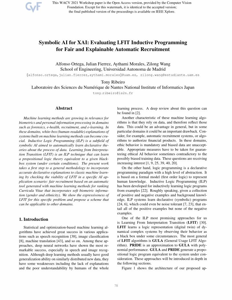
Figure 1 shows the architecture of our proposed ap-

78

Output classes (target) = {0,1}

Input features (variables)

Declarative explanation

(propositional logic fragment)

𝒱 = v1, v2, v3v1 binary, v2 and v3 ∈ ℕClassifier seen as black-box system (input/outputs)

Examples (two inputs 𝒱𝐴 and 𝒱𝐵)

𝒱𝐴 = v1 = 0v2 = 5v3 = 2 𝒱𝐵 = v1 = 1v2 = 3v3 = 0

Note that the explanation reveals that the output only depends on v1

1

Logical equivalent system

(White-box Digital Twin of

the Black-box Classifier)

LFIT (PRIDE)

2

target(0) :- v1 0 .target(1) :- v1 1 .

3

Figure 1: Architecture of the proposed approach for generating an explanation of a given black-box Classifier (1) using

PRIDE (2) with a toy example (3). Note that the resulting explanations generated by PRIDE are in propositional logic.

proach for generating white-box explanations using PRIDE

of a given black-box classifier.

The main contributions of this work are:

• We have proposed a method to provide declarative ex-

planations using PRIDE about the classification pro-

cess made by an algorithm automatically learnt by a

neural architecture in a typical machine learning sce-

nario. Our approach guarantees the logical equivalence

between the explanations and the algorithm with re-

spect to the data used to feed PRIDE. It does not de-

pend on any particular characteristic of the domain, so

it could be applied to any problem.

• We have checked the expressive power of these ex-

planations by experimenting in a multimodal machine

learning testbed around automatic recruitment includ-

ing different biases (by gender and ethnicity).

The rest of the paper is structured as follows: Sec. 2 sum-

marizes the related relevant literature. Sec. 3 describes our

methodology including LFIT, GULA, and PRIDE. Sec. 4

presents the experimental framework including the datasets

and experiments conducted. Sec. 5 presents our results. Fi-

nally Secs. 6, 7 and 8 respectively discuss our work and

describe our conclusions and further research lines.

2. Related Works: Inductive Programming for

XAI

Some meta-heuristics approaches (as genetic algorithms)

have been used to automatically generate programs. Ge-

netic programming (GP) was introduced by Koza [15] for

automatically generating LISP expressions for given tasks

expressed as pairs input/output. This is, in fact, a typical

machine learning scenario. GP was extended by the use of

formal grammars to allow to generate programs in any arbi-

trary language keeping not only syntactic correctness [27]

but also semantic properties [28]. Algorithms expressed

in any language are declarative versions of the concepts

learnt what makes evolutionary automatic programming al-

gorithms machine learners with good explainability.

Declarative programming paradigms (functional, logi-

cal) are as old as computer science and are implemented

in multiple ways, e.g.: LISP [13], Prolog [5], Datalog [11],

Haskell [41], and Answer Set Programs (ASP) [10].

Of particular interest for us within declarative paradigms

is logic programming, and in particular first order logic pro-

gramming, which is based on the Robinson’s resolution in-

ference rule that automates the reasoning process of de-

ducing new clauses from a first order theory [17]. Intro-

ducing examples and counter examples and combining this

scheme with the ability of extending the initial theory with

new clauses it is possible to automatically induce a new

theory that (logically) entails all of the positive examples

but none of the negative examples. The underlying theory

from which the new one emerges is considered background

knowledge. This is the hypothesis of Inductive Logic Pro-

gramming (ILP, [21, 6]) that has received a great research

effort in the last two decades. Recently, these approaches

have been extended to make them noise tolerant (in order

to overcome one of the main drawbacks of ILP vs statisti-

cal/numerical approaches when facing bad-labeled or noisy

examples [23]).

79

Other declarative paradigms are also compatible with

ILP, e.g., MagicHaskeller (that implements [14]) with the

functional programming language Haskell, and Inductive

Learning of Answer Set Programs (ILASP) [16].

It has been previously mentioned that ILP implies some

kind of search in spaces that can become huge. This search

can be eased by hybridising with other techniques, e.g., [26]

introduces GA-Progol that applies evolutive techniques.

Within ILP methods we have identified LFIT as spe-

cially relevant for explainable AI (XAI). In the next sec-

tion we will describe the fundamentals of LFIT and its

PRIDE implementation, which will be tested experimen-

tally for XAI in the experiments that will follow.

2.1. Learning From Interpretation Transition(LFIT)

Learning From Interpretation Transition (LFIT) [12] has

been proposed to automatically construct a model of the dy-

namics of a system from the observation of its state transi-

tions. Given some raw data, like time-series data of gene

expression, a discretization of those data in the form of state

transitions is assumed. From those state transitions, accord-

ing to the semantics of the system dynamics, several infer-

ence algorithms modeling the system as a logic program

have been proposed. The semantics of a system’s dynamics

can indeed differ with regard to the synchronism of its vari-

ables, the determinism of its evolution and the influence of

its history.

The LFIT framework proposes several modeling and

learning algorithms to tackle those different semantics. To

date, the following systems have been tackled: memory-

less deterministic systems [12], systems with memory [35],

probabilistic systems [19] and their multi-valued extensions

[36, 18]. The work [37] proposes a method that allows to

deal with continuous time series data, the abstraction itself

being learned by the algorithm.

In [31, 33], LFIT was extended to learn systems dynam-

ics independently of its update semantics. That extension

relies on a modeling of discrete memory-less multi-valued

systems as logic programs in which each rule represents that

a variable possibly takes some value at the next state, ex-

tending the formalism introduced in [12, 34]. The represen-

tation in [31, 33] is based on annotated logics [4, 3]. Here,

each variable corresponds to a domain of discrete values.

In a rule, a literal is an atom annotated with one of these

values. It allows to represent annotated atoms simply as

classical atoms and thus to remain at a propositional level.

This modeling allows to characterize optimal programs in-

dependently of the update semantics. It allows to model the

dynamics of a wide range of discrete systems including our

domain of interest in this paper. LFIT can be used to learn

an equivalent propositional logic program that provides ex-

planation for each given observation.

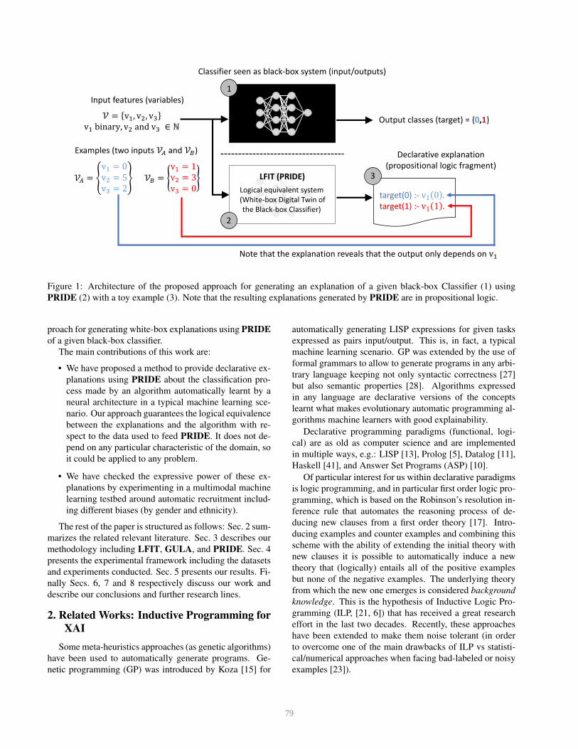
Figure 2: Experimental framework: PRIDE is fed with all

the data available (train + test) for increasing the accuracy

of the equivalence. In our experiments we consider the clas-

sifier (see [29] for details) as a black box to perform regres-

sion from input resume attributes (atts.) to output labels

(recruitment scores labelled by human resources experts).

LFIT gets a digital twin to the neural network providing

explainability (as human-readable white-box rules) to the

neural network classifier.

3. Methods

3.1. General Methodology

Figure 2 graphically describes our proposed approach

to generate explanations using LFIT of a given black-box

classifier. We can see there our purpose to get declarative

explanations in parallel (in a kind of white-blox digital twin)

to a given neural network classifier. In the present work, for

our experiments we have used the same neural network and

datasets described in [29] but excluding the face images as

it is explained in the following sections.

3.2. PRIDE Implementation of LFIT

GULA [31, 33] and PRIDE [32] are particular imple-

mentations of the LFIT framework [12]. In the present sec-

tion we introduce notation and describe the fundamentals of

both methods.

In the following, we denote by N := {0, 1, 2, ...} the set

of natural numbers, and for all k, n ∈ N, Jk;nK := {i ∈ N |k ≤ i ≤ n} is the set of natural numbers between k and nincluded. For any set S, the cardinal of S is denoted |S| and

the power set of S is denoted ℘(S).

80

Let V = {v1, . . . , vn} be a finite set of n ∈ N vari-

ables, Val the set in which variables take their values and

dom : V → ℘(Val) a function associating a domain to each

variable. The atoms of MVL (multi-valued logic) are of

the form vval where v ∈ V and val ∈ dom(v). The set of

such atoms is denoted byAVdom

= {vval ∈ V ×Val | val ∈dom(v)} for a given set of variables V and a given domain

function dom. In the following, we work on specific V and

dom that we omit to mention when the context makes no

ambiguity, thus simply writing A for AVdom

.

Example 1 For a system of 3 variables, the typical set

of variables is V = {a, b, c}. In general, Val =N so that domains are sets of natural integers, for in-

stance: dom(a) = {0, 1}, dom(b) = {0, 1, 2} and

dom(c) = {0, 1, 2, 3}. Thus, the set of all atoms is:

A = {a0, a1, b0, b1, b2, c0, c1, c2, c3}.

AMVL rule R is defined by:

R = vval00 ← vval11 ∧ · · · ∧ vvalmm (1)

where ∀i ∈ J0;mK, vvalii ∈ A are atoms in MVL so that

every variable is mentioned at most once in the right-hand

part: ∀j, k ∈ J1;mK, j 6= k ⇒ vj 6= vk. Intuitively, the rule

R has the following meaning: the variable v0 can take the

value val0 in the next dynamical step if for each i ∈ J1;mK,

variable vi has value vali in the current dynamical step.

The atom on the left-hand side of the arrow is called the

head of R and is denoted h(R) := vval00 . The notation

var(h(R)) := v0 denotes the variable that occurs in h(R).The conjunction on the right-hand side of the arrow is called

the body of R, written b(R) and can be assimilated to the

set {vval11 , . . . , vvalmm }; we thus use set operations such as

∈ and ∩ on it. The notation var(b(R)) := {v1, · · · , vm}denotes the set of variables that occurs in b(R). More gen-

erally, for all set of atoms X ⊆ A, we denote var(X) :={v ∈ V | ∃val ∈ dom(v), vval ∈ X} the set of variables

appearing in the atoms of X . A multi-valued logic program

(MVLP) is a set ofMVL rules.

Definition 1 introduces a domination relation between

rules that defines a partial anti-symmetric ordering. Rules

with the most general bodies dominate the other rules. In

practice, these are the rules we are interested in since they

cover the most general cases.

Definition 1 (Rule Domination) Let R1, R2 be twoMVLrules. The rule R1 dominates R2, written R2 ≤ R1 if

h(R1) = h(R2) and b(R1) ⊆ b(R2).

In [33], the set of variables is divided into two disjoint

subsets: T (for targets) and F (for features). It allows to

define dynamicMVLP which capture the dynamics of the

problem we tackle in this paper.

Definition 2 (DynamicMVLP) Let T ⊂ V and F ⊂ Vsuch that F = V \T . A DMVLP P is aMVLP such that

∀R ∈ P, var(h(R)) ∈ T and ∀vval ∈ b(R), v ∈ F .

The dynamical system we want to learn the rules of is

represented by a succession of states as formally given by

Definition 3. We also define the “compatibility” of a rule

with a state in Definition 4.

Definition 3 (Discrete state) A discrete state s on T (resp.

F) of a DMVLP is a function from T (resp. F) to N, i.e.

it associates an integer value to each variable in T (resp.

F). It can be equivalently represented by the set of atoms

{vs(v) | v ∈ T (resp. F)} and thus we can use classical set

operations on it. We write ST (resp. SF ) to denote the set

of all discrete states of T (resp. F), and a couple of states

(s, s′) ∈ SF × ST is called a transition.

Definition 4 (Rule-state matching) Let s ∈ SF . The

MVL rule R matches s, written R ⊓ s, if b(R) ⊆ s.

The notion of transition in LFIT correspond to a data

sample in the problem we tackle in this paper: a couple fea-

tures/targets. When a rule match a state it can be considered

as a possible explanation to the corresponding observation.

The final program we want to learn should both:

• match the observations in a complete (all observations

are explained) and correct (no spurious explanation)

way;

• represent only minimal necessary interactions (accord-

ing to Occam’s razor: no overly-complex bodies of

rules)

GULA [31, 33] and PRIDE [32] can produce such pro-

grams.

Formally, given a set of observations T , GULA [31, 33]

and PRIDE [32] will learn a set of rules P such that all

observations are explained: ∀(s, s′) ∈ T, ∀vval ∈ s′, ∃R ∈P,R ⊓ s, h(R) = vval. All rules of P are correct w.r.t.

T : ∀R ∈ P, ∀(s1, s2) ∈ T,R ⊓ s1 =⇒ ∃(s1, s3) ∈T, h(R) ∈ s3 (if T is deterministic, s2 = s3). All rules are

minimal w.r.t. F : ∀R ∈ P, ∀R′ ∈MVLP, R′ correct w.r.t.

T it holds that R ≤ R′ =⇒ R′ = R.

The possible explanations of an observation are the rules

that match the feature state of this observation. The body of

the rules gives minimal condition over feature variables to

obtain its conclusions over a target variable. Multiple rules

can match the same feature state, thus multiple explanations

can be possible. Rules can be weighted by the number of

observations they match to assert their level of confidence.

Output programs of GULA and PRIDE can also be used in

order to predict and explain from unseen feature states by

learning additional rules that encode when a target variable

value is not possible as shown in the experiments of [33].

81

4. Experimental Framework

4.1. Dataset

For testing the capability of PRIDE to generate explana-

tions in machine learning domains we have designed several

experiments using the FairCVdb dataset [29].

FairCVdb comprises 24,000 synthetic resume profiles.

Each resume includes 12 features (vi) related to the can-

didate merits, 2 demographic attributes (gender and three

ethnicity groups), and a face photograph. In our experi-

ments, we discarded the face image for simplicity (unstruc-

tured image data will be explored in future work). Each of

the profiles includes three target scores (T ) generated as a

linear combination of the 12 features:

T = β +

12∑

i=1

αi · vi, (2)

where αi is a weighting factor for each of the merits (see

[29] for details): i) unbiased score (β = 0); ii) gender-

biased scores (β = 0.2 for male and β = 0 for female

candidates); and iii) ethnicity-biased scores (β = 0.0, 0.15and 0.3 for candidates from ethnic groups 1, 2 and 3 respec-

tively). Thus we intentionally introduce bias in the candi-

date scores. From this point on we will simplify the name

of the attributes considering g for gender, e for ethnic group

and i1 to i12 for the rest of input attributes. In addition

to the bias previously introduced, some other random bias

was introduced relating some attributes and gender to sim-

ulate real social dynamics. The attributes concerned were

i3 and i7. Note that merits were generated without bias, as-

suming an ideal scenario where candidate competencies do

not depend on their gender of ethnic group. For the current

work we have used only discrete values for each attribute

discretizing one attribute (experience to take values from 0

to 5, the higher the better) and the scores (from 0 to 3) that

were real valued in [29].

4.2. Experimental Protocol: Towards DeclarativeExplanations

We have experimented with PRIDE on the FairCVdb

dataset described in the previous section.

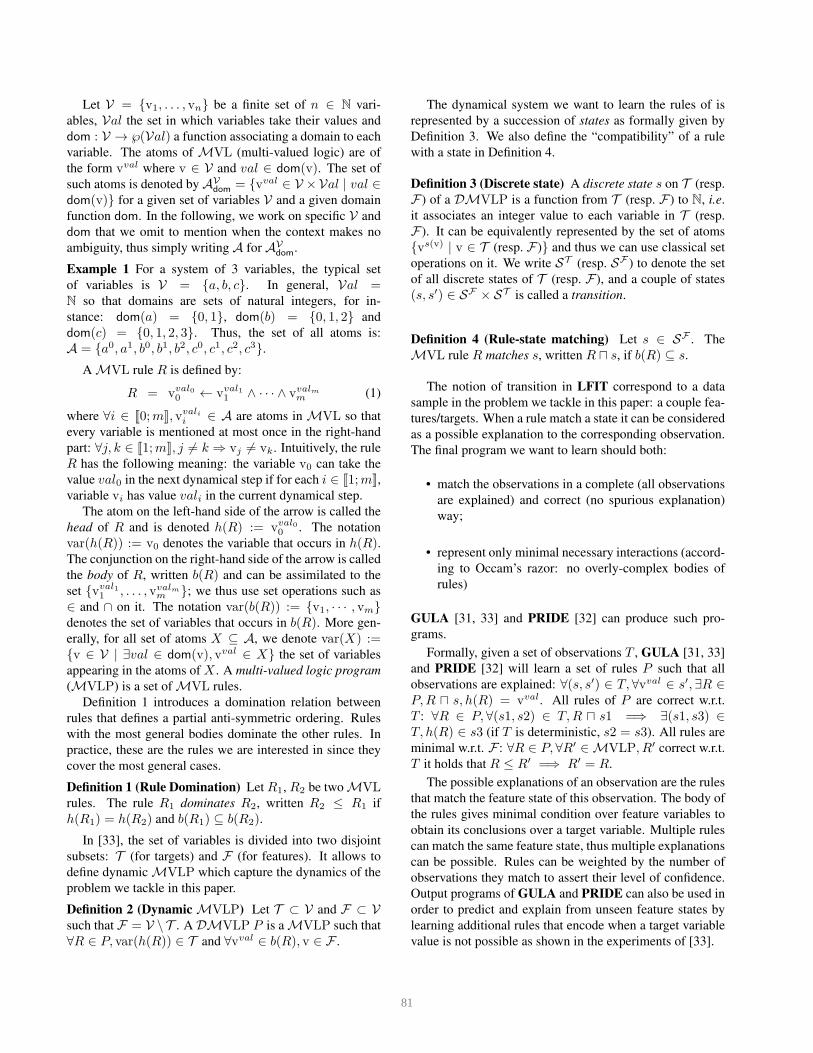
Figure 3 shows names and explains the scenarios consid-

ered in our experiments. In [29], researchers demonstrate

that an automatic recruitment algorithm based on multi-

modal machine learning reproduces existing biases in the

target functions even if demographic information was not

available as input (see [29] for details). Our purpose in the

experiments is to obtain a declarative explanation capable

of revealing those biases.

Figure 3: Structure of the experimental tests. There are 4

datasets for analysing gender (named g) and ethnicity (e)

bias separately. Apart from gender and ethnicity there are

12 other input attributes (named from i1 to i12). There is a

couple of (biased and unbiased) datasets for each one: gen-

der and ethnicity. We have studied the input attributes by

increasing complexity starting with i1 and i2 and adding

one at each time. So, for each couple we have considered

11 different scenarios (named from s1 to s11). This fig-

ure shows their structure (si is included in all sj for which

i < j).

5. Results

5.1. Example of Declarative Explanation

Listing 1 shows a fragment generated with the proposed

methods for scenario s1 for gender-biased scores. We have

chosen a fragment that fully explains how a CV is scored

with the value 3 for scenario 1. Scenario 1 takes into ac-

count the input attributes gender, education and experience.

The first clause (rule), for example, says that if the value of

a CV for the attribute gender is 1 (female), for education is 5

(the highest), and for experience is 3, then this CV receives

the highest score (3).

The resulting explanation is a propositional logic frag-

ment equivalent to the classifier for the data seen. It can

be also understood as a set of rules with the same behav-

ior. From the viewpoint of explainable AI, this resulting

fragment can be understood by an expert in the domain and

used to generate new knowledge about the scoring of CVs.

1

2 scores(3) :- gender(1),

3 education(5),

4 experience(3).

5 scores(3) :- education(4),

6 experience(3).

Listing 1: Fragment of explanation for scoring 3

5.2. Quantitative Results: Identifying Biases

Our quantitative results are divided in two parts. The first

part is based on the fact that, in the biased experiments, if

82

gender(0) appears more frequently than gender(1) in the

rules, then that would lead to higher scores for gender(0).In the second quantitative experimental part we will show

the influence of bias in the distribution of attributes.

5.2.1 Biased attributes in rules

We first define Partial Weight PW as follows. For any pro-

gram P and two atoms vvali

0

0 and vval

j1

1 , where vali0 ∈ val0

and vali1 ∈ val1, define S = ∀R ∈ P ∧ vvali

0

0 ∈ h(R) ∧

vval

j1

1 ∈ b(R). Then we have: PWvval

j1

1

(vval0

0

0 ) = |S|. A

more accurate PW could be defined, for example, setting

different weights for rules with different length. But for our

purpose, the frequency is enough. In our analysis, the num-

ber of examples for compared scenarios are consistent.

Depending on PW , we define Global Weight GW

as follows. For any program P and vval

j1

1 , we have:

GWvval

j1

1

=∑

vali0∈val0

PWvval

j1

1

(vvali

0

0 ) · vali0. The

GWvval

j1

1

is a weighted addition of all the values of the out-

put, and the weight, in our case, is the value of scores.

This analysis was performed only on scenario s11, com-

paring unbiased and gender- and ethnicity-biased scores.

We have observed a similar behavior of both parameters:

Partial and Global Weights. In unbiased scenarios the

distributions of the occurrences of each value could be

considered statistically the same (between gender(0) and

gender(1) and among ethnicity(0), ethnicity(1) and ethnic-

ity(2)). Nevertheless in biased datasets the occurrences of

gender(0) and ethnic(0) for higher scores is significantly

higher. The maximum difference even triplicates the oc-

currences of the other values.

For the Global Weights, for example, the maximum dif-

ferences in the number of occurrences, without and with

bias respectively, for higher scores expressed as % increases

from 48.8% to 78.1% for gender(0) while for gender(1)

decreases from 51.2% to 21.9%. In the case of ethnicity,

it increases from 33.4% to 65.9% for ethnic(0), but de-

creases from 33.7% to 19.4% for ethnic(1) and from 32.9%to 14.7% for ethnic(2).

5.2.2 Distribution of biased attributes

We now define freqp1(a) as the frequency of attribute a in

P1. The normalized percentage for input a is: NPp1(a) =

freqp1(a)/

∑x∈input freqp1

(x) and the percentage of the

absolute increment for each input from unbiased exper-

iments to its corresponding biased ones is defined as:

AIPp1,p2(a) = (freqp1

(a)− freqp2(a))/freqp2

(a).

In this approach we have taken into account all the sce-

narios (from s1 to s11) for both gender and ethnicity.

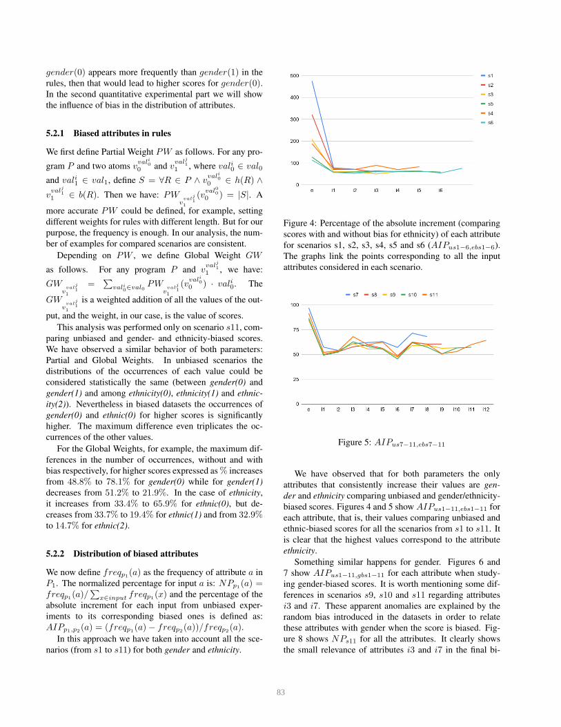
Figure 4: Percentage of the absolute increment (comparing

scores with and without bias for ethnicity) of each attribute

for scenarios s1, s2, s3, s4, s5 and s6 (AIPus1−6,ebs1−6).

The graphs link the points corresponding to all the input

attributes considered in each scenario.

Figure 5: AIPus7−11,ebs7−11

We have observed that for both parameters the only

attributes that consistently increase their values are gen-

der and ethnicity comparing unbiased and gender/ethnicity-

biased scores. Figures 4 and 5 show AIPus1−11,ebs1−11 for

each attribute, that is, their values comparing unbiased and

ethnic-biased scores for all the scenarios from s1 to s11. It

is clear that the highest values correspond to the attribute

ethnicity.

Something similar happens for gender. Figures 6 and

7 show AIPus1−11,gbs1−11 for each attribute when study-

ing gender-biased scores. It is worth mentioning some dif-

ferences in scenarios s9, s10 and s11 regarding attributes

i3 and i7. These apparent anomalies are explained by the

random bias introduced in the datasets in order to relate

these attributes with gender when the score is biased. Fig-

ure 8 shows NPs11 for all the attributes. It clearly shows

the small relevance of attributes i3 and i7 in the final bi-

83

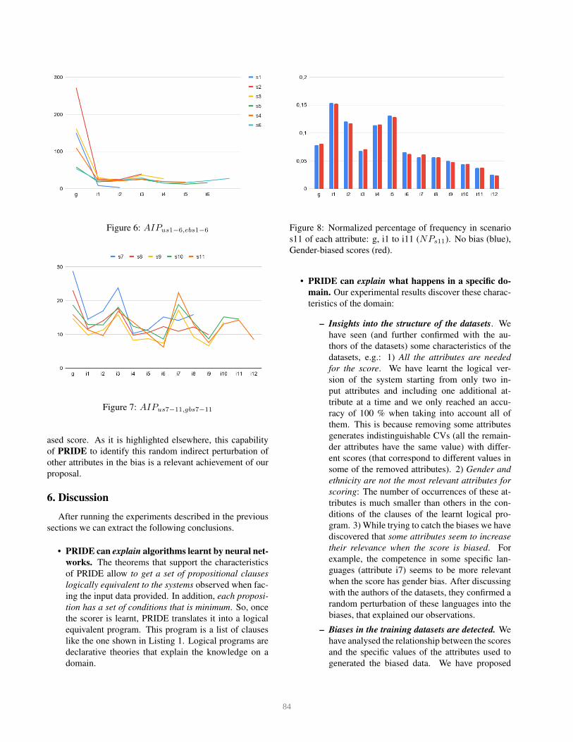
Figure 6: AIPus1−6,ebs1−6

Figure 7: AIPus7−11,gbs7−11

ased score. As it is highlighted elsewhere, this capability

of PRIDE to identify this random indirect perturbation of

other attributes in the bias is a relevant achievement of our

proposal.

6. Discussion

After running the experiments described in the previous

sections we can extract the following conclusions.

• PRIDE can explain algorithms learnt by neural net-

works. The theorems that support the characteristics

of PRIDE allow to get a set of propositional clauses

logically equivalent to the systems observed when fac-

ing the input data provided. In addition, each proposi-

tion has a set of conditions that is minimum. So, once

the scorer is learnt, PRIDE translates it into a logical

equivalent program. This program is a list of clauses

like the one shown in Listing 1. Logical programs are

declarative theories that explain the knowledge on a

domain.

Figure 8: Normalized percentage of frequency in scenario

s11 of each attribute: g, i1 to i11 (NPs11). No bias (blue),

Gender-biased scores (red).

• PRIDE can explain what happens in a specific do-

main. Our experimental results discover these charac-

teristics of the domain:

– Insights into the structure of the datasets. We

have seen (and further confirmed with the au-

thors of the datasets) some characteristics of the

datasets, e.g.: 1) All the attributes are needed

for the score. We have learnt the logical ver-

sion of the system starting from only two in-

put attributes and including one additional at-

tribute at a time and we only reached an accu-

racy of 100 % when taking into account all of

them. This is because removing some attributes

generates indistinguishable CVs (all the remain-

der attributes have the same value) with differ-

ent scores (that correspond to different values in

some of the removed attributes). 2) Gender and

ethnicity are not the most relevant attributes for

scoring: The number of occurrences of these at-

tributes is much smaller than others in the con-

ditions of the clauses of the learnt logical pro-

gram. 3) While trying to catch the biases we have

discovered that some attributes seem to increase

their relevance when the score is biased. For

example, the competence in some specific lan-

guages (attribute i7) seems to be more relevant

when the score has gender bias. After discussing

with the authors of the datasets, they confirmed a

random perturbation of these languages into the

biases, that explained our observations.

– Biases in the training datasets are detected. We

have analysed the relationship between the scores

and the specific values of the attributes used to

generated the biased data. We have proposed

84

a simple mathematical model based on the ef-

fective weights of the attributes that concludes

that higher values of the scores correspond to

the same specific values of gender (for gender

bias) and ethnic group (for ethnicity bias). On the

other hand, we have performed an exhaustive se-

ries of experiments to analyse the increase of the

presence of the gender and ethnicity in the condi-

tions of the clauses of the learnt logical program

(comparing the unbiased and biased versions).

Our overall conclusion is that LFIT, and in particular

PRIDE, is able to offer explanations to the algorithm learnt

in the domain under consideration. The resulting explana-

tion is, as well, expressive enough to catch training biases

in the models learnt with neural networks.

7. Conclusions

The main goal of this paper was to check if ILP (and

more specifically LFIT with PRIDE) could be useful to pro-

vide declarative explanations in machine learning by neural

networks.

The domain selected for our experiments in this first

entry to the topic is one in which the explanations of the

learned models’ outputs are specially relevant: automatic

recruitment algorithms. In this domain, ethic behavior is

needed, no spurious biases are allowed. For this purpose,

a pack of synthetically generated datasets has been used.

The datasets contain resumes (CVs) used in [29] for testing

the ability of deep learning approaches to reproduce and re-

move biases present in the training datasets. In the present

work, different input attributes (including the resume owner

merits, gender, and ethnicity) are used to score each CV

automatically using a neural network. Different setups are

considered to introduce artificial gender- and ethnicity-bias

in the learning process of the neural network. In [29] face

images were also used and the relationship between these

pictures and the biases was studied (it seems clear that from

the face you should be able to deduce the gender and ethnic

group of a person). Here we have removed images because

PRIDE is more efficient with pure discrete information.

Our main goal indicated above translates into these two

questions: Is PRIDE expressive enough to explain how the

program learnt by deep-learning approaches works? Does

PRIDE catch biases in the deep-learning processes? We

have given positive answer to both questions.

8. Further Research Lines

• Increasing understandability. Two possibilities

could be considered in the future: 1) to ad hoc post-

process the learnt program for translating it into a more

abstract form, or 2) to increase the expressive power of

the formal model that supports the learning engine us-

ing, for example, ILP based on first order logic.

• Adding predictive capability. PRIDE is actually

not aimed to predict but to explain (declaratively) by

means of a digital twin of the observed systems. Nev-

ertheless, it is not really complicated to extend PRIDE

functionality to predict. It should be necessary to

change the way in which the result is interpreted as

a logical program: mainly by adding mechanisms to

chose the most promising rule when more than one is

applicable.

Our plan is to test an extended-to-predict PRIDE ver-

sion to this same domain and compare the result with

the classifier generated by deep learning algorithms.

• Handling numerical inputs. [29] included as input

the images of the faces of the owners of the CVs. Al-

though some variants to PRIDE are able to cope with

numerical signals, the huge amount of information as-

sociated with images implies performance problems.

Images are a typical input format in real deep learn-

ing domains. We would like to add some automatic

pre-processing step for extracting discrete information

(such as semantic labels) from input images. We are

motivated by the success of systems with similar ap-

proaches but different structure like [42].

• Measuring the accuracy and performance of the ex-

planations. As far as the authors know there is no

standard procedure to evaluate and compare different

explainability approaches. We will incorporate in fu-

ture versions some formal metric.

9. Acknowledgements

This work has been supported by projects: PRIMA

(H2020-MSCA-ITN-2019-860315), TRESPASS-ETN

(H2020-MSCA-ITN-2019-860813), IDEA-FAST (IMI2-

2018-15-853981), BIBECA (RTI2018-101248-B-I00

MINECO/FEDER), RTI2018-095232-B-C22 MINECO,

and Accenture.

References

[1] A. Acien, A. Morales, R. Vera-Rodriguez, I. Bartolome, and

J. Fierrez. Measuring the gender and ethnicity bias in deep

models for face recognition. In Iberoamerican Congress

on Pattern Recognition (IBPRIA), pages 584–593. Springer,

2018.

[2] Alejandro Barredo Arrieta, Natalia Dıaz Rodrıguez,

Javier Del Ser, Adrien Bennetot, Siham Tabik, Alberto Bar-

bado, Salvador Garcıa, Sergio Gil-Lopez, Daniel Molina,

Richard Benjamins, Raja Chatila, and Francisco Herrera.

Explainable artificial intelligence (XAI): concepts, tax-

onomies, opportunities and challenges toward responsible

AI. Information Fusion, 58:82–115, 2020.

85

[3] H. A Blair and V.S. Subrahmanian. Paraconsistent founda-

tions for logic programming. Journal of Non-classical Logic,

5(2):45–73, 1988.

[4] H. A. Blair and V.S. Subrahmanian. Paraconsistent logic pro-

gramming. Theoretical Computer Science, 68(2):135 – 154,

1989.

[5] I. Bratko. Prolog Programming for Artificial Intelligence,

4th Edition. Addison-Wesley, 2012.

[6] A. Cropper and S. H. Muggleton. Learning efficient logic

programs. Machine Learning, 108(7):1063–1083, 2019.

[7] W. Z. Dai, S. H. Muggleton, and Z. H. Zhou. Logical vision:

Meta-interpretive learning for simple geometrical concepts.

2015.

[8] J. Deng, W. Dong, R. Socher, L.-J. Li, K. Li, and L. Fei-Fei.

ImageNet: A Large-Scale Hierarchical Image Database. In

CVPR, 2009.

[9] P. Drozdowski, C. Rathgeb, A. Dantcheva, N. Damer, and

C. Busch. Demographic bias in biometrics: A survey on an

emerging challenge. IEEE Transactions on Technology and

Society, 2020.

[10] M. Gebser, R. Kaminski, B. Kaufmann, and T. Schaub. An-

swer Set Solving in Practice. Synthesis Lectures on Artifi-

cial Intelligence and Machine Learning. Morgan & Claypool

Publishers, 2012.

[11] S. S. Huang, T. Jeffrey Green, and B. T. Loo. Datalog and

emerging applications: an interactive tutorial. In Timos K.

Sellis, Renee J. Miller, Anastasios Kementsietsidis, and Yan-

nis Velegrakis, editors, Proc. of the ACM SIGMOD Intl.

Conf. on Management of Data, pages 1213–1216, June 2011.

[12] K. Inoue, T. Ribeiro, and C. Sakama. Learning from inter-

pretation transition. Machine Learning, 94(1):51–79, 2014.

[13] Guy L. Steele Jr. Common LISP: The Language, 2nd Edition.

Digital Pr., 1990.

[14] S. Katayama. Systematic search for lambda expressions. In

M. C. J. D. van Eekelen, editor, Revised Selected Papers from

the Sixth Symposium on Trends in Functional Programming,

volume 6 of Trends in Functional Programming, pages 111–

126. Intellect, September 2005.

[15] J.R. Koza. Genetic Programming. MIT Press, 1992.

[16] M. Law. Inductive learning of answer set programs., 2018.

PhD. Imperial College London.

[17] J. W. Lloyd. Foundations of Logic Programming, 2nd Edi-

tion. Springer, 1987.

[18] D. Martınez, G. Alenya, C. Torras, T. Ribeiro, and K. Inoue.

Learning relational dynamics of stochastic domains for plan-

ning. In Proceedings of the 26th International Conference on

Automated Planning and Scheduling, 2016.

[19] D. Martınez Martınez, T. Ribeiro, K. Inoue, G. Alenya Ribas,

and C. Torras. Learning probabilistic action models from

interpretation transitions. In Proceedings of the Technical

Communications of the 31st International Conference on

Logic Programming (ICLP 2015), pages 1–14, 2015.

[20] Aythami Morales, Julian Fierrez, Ruben Vera-Rodriguez,

and Ruben Tolosana. Sensitivenets: Learning agnostic repre-

sentations with application to face recognition. IEEE Trans-

actions on Pattern Analysis and Machine Intelligence, 2021.

[21] S. Muggleton. Inductive logic programming. In S. Arikawa,

Sh. Goto, S. Ohsuga, and T. Yokomori, editors, Proc. First

Intl. Workshop on Algorithmic Learning Theory, pages 42–

62. Springer, October 1990.

[22] S. Muggleton. Inductive logic programming. New Genera-

tion Computing, 8(4):295–318, 1991.

[23] S. Muggleton, W.-Z. Dai, C. Sammut, A. Tamaddoni-

Nezhad, J. Wen, and Z.-H. Zhou. Meta-interpretive learning

from noisy images. Machine Learning, 107(7):1097–1118,

2018.

[24] S. H. Muggleton, D. Lin, N. Pahlavi, and A. Tamaddoni-

Nezhad. Meta-interpretive learning: application to grammat-

ical inference. Machine Learning, 94(1):25–49, 1994.

[25] S. Nagpal, M. Singh, R. Singh, M. Vatsa, and N.i K. Ratha.

Deep learning for face recognition: Pride or prejudiced?

CoRR, abs/1904.01219, 2019.

[26] A. T. Nezhad. Logic-based machine learning using a

bounded hypothesis space: the lattice structure, refinement

operators and a genetic algorithm approach, August 2013.

PhD, Imperial College London.

[27] M. O’Neill and R. Conor. Grammatical Evolution - Evolu-

tionary Automatic Programming in an Arbitrary Language,

volume 4 of Genetic programming. Kluwer, 2003.

[28] A. Ortega, M. de la Cruz, and M. Alfonseca. Christiansen

grammar evolution: Grammatical evolution with semantics.

IEEE Trans. Evol. Comput., 11(1):77–90, 2007.

[29] A. Pena, I. Serna, A. Morales, and J. Fierrez. Bias in mul-

timodal AI: testbed for fair automatic recruitment. In Proc.

IEEE/CVF Conf. on Computer Vision and Pattern Recogni-

tion (CVPR) Workshops, pages 129–137, June 2020.

[30] T. Ribeiro. Studies on learning dynamics of systems from

state transitions, 2015. PhD.

[31] T. Ribeiro, M. Folschette, M. Magnin, O. Roux, and K. In-

oue. Learning dynamics with synchronous, asynchronous

and general semantics. In International Conference on In-

ductive Logic Programming, pages 118–140. Springer, 2018.

[32] T. Ribeiro, M. Folschette, L. Trilling, N. Glade, K. Inoue, M.

Magnin, and O. Roux. Les enjeux de l’inference de modeles

dynamiques des systemes biologiques a partir de series tem-

porelles. In C. Lhoussaine and E. Remy, editors, Approches

symboliques de la modelisation et de l’analyse des systemes

biologiques. ISTE Editions, 2020. In edition.

[33] T. Ribeiro, M. Folschette, M.and Magnin, and K. Inoue.

Learning any semantics for dynamical systems represented

by logic programs. working paper or preprint, Sept. 2020.

[34] T. Ribeiro and K. Inoue. Learning prime implicant condi-

tions from interpretation transition. In Inductive Logic Pro-

gramming, pages 108–125. Springer, 2015.

[35] T. Ribeiro, M. Magnin, K. Inoue, and C. Sakama. Learning

delayed influences of biological systems. Frontiers in Bio-

engineering and Biotechnology, 2:81, 2015.

[36] T. Ribeiro, M. Magnin, K. Inoue, and C. Sakama. Learn-

ing multi-valued biological models with delayed influence

from time-series observations. In 2015 IEEE 14th Inter-

national Conference on Machine Learning and Applications

(ICMLA), pages 25–31, Dec 2015.

86

[37] T. Ribeiro, S. Tourret, M. Folschette, M. Magnin, D. Borzac-

chiello, F. Chinesta, O. Roux, and K. Inoue. Inductive learn-

ing from state transitions over continuous domains. In N.

Lachiche and C. Vrain, editors, Inductive Logic Program-

ming, pages 124–139. Springer, 2018.

[38] A. Senior, V. Vanhoucke, P. Nguyen, and T. Sainath. Deep

neural networks for acoustic modeling in speech recognition.

IEEE Signal Processing magazine, 2012.

[39] Ignacio Serna, Aythami Morales, Julian Fierrez, Manuel Ce-

brian, Nick Obradovich, and Iyad Rahwan. Algorithmic dis-

crimination: Formulation and exploration in deep learning-

based face biometrics. In AAAI Workshop on Artificial Intel-

ligence Safety (SafeAI), February 2020.

[40] Ignacio Serna, Alejandro Pena, Aythami Morales, and Julian

Fierrez. InsideBias: Measuring bias in deep networks and

application to face gender biometrics. In IAPR Intl. Conf. on

Pattern Recognition (ICPR), January 2021.

[41] S. J. Thompson. Haskell - The Craft of Functional Program-

ming, 3rd Edition. Addison-Wesley, 2011.

[42] D. Varghese and A. Tamaddoni-Nezhad. One-shot rule learn-

ing for challenging character recognition. In S. Moschoyian-

nis, P. Fodor, J. Vanthienen, D. Inclezan, Ni. Nikolov, F.

Martın-Recuerda, and I. Toma, editors, Proc. of the 14th Intl.

Rule Challenge, volume 2644 of CEUR Workshop Proceed-

ings, pages 10–27, June 2020.

[43] Y. Wu, M. Schuster, Z. Chen, Q. V. Le, M. Norouzi, W.

Macherey, and J Klingner. Google’s neural machine transla-

tion system: Bridging the gap between human and machine

translation. arXiv preprint arXiv:1609.08144, 2016.

87