Switching fuzzy tracking control for mobile robots under curvature constraints

Abstract—In this paper a switching fuzzy logic controller for mobile robots with a bounded curvature

constraint is presented. The controller tracks piece-wise linear paths which are an approximation of the

feasible smooth reference path. The controller is constructed through the use of a map which transforms the

problem to a simpler one; namely the tracking of straight lines. This allows the use of an existing fuzzy tracker

deployed in a previous work, and its simplification leading to a 70% rule reduction. Simulation results and a

comparison analysis with existing trackers are also presented along with some stability considerations on the

impulsive error dynamics which emerge.

Index Terms — Path Tracking, Non-Holonomic Mobile Robots, Strip-Wise Affine Map, Switching Control,

Fuzzy Logic, Impulsive Systems

I. INTRODUCTION

Path tracking is an essential part of the navigation process of every mobile robot that follows the

deliberative control paradigm. In this setting, the robot uses state and environment information in order to

plan ahead its movements. On the contrary, reactive control systems employ a tight coupling between

perception and motor action leading to more timely responses but lacking the predictive capabilities of the

former.

In a typical case, the path is provided by a path planner that calculates a feasible path between the start

and goal positions. The planner can take into account special restrictions such as the distance from

obstacles, kinematic and dynamic constraints of the robotic system, total travel length etc. The path is

then presented to the path tracker that performs the actual movement. The aim of the tracker is to navigate

the robot on the path, accounting for disturbances in the moving phase, e.g., wheel slippage, uneven

terrain, localization uncertainty etc. The study of path tracking has produced a vast amount of research

literature ranging from classical control approaches (Altafini, 1999; Kamga & Rachid, 1997; Kanayama

& Fahroo, 1997), to nonlinear control methodologies (Altafini, 2002; Egerstedt, Hu, & Stotsky, 1998;

Koh & Cho, 1994; Samson, 1995; Wit, Crane, & Armstrong, 2004) to intelligent control strategies

(Abdessemed, Benmahammed, & Monacelli, 2004; Antonelli, Chiaverini, & Fusco, 2007; Baltes & Otte,

1999; Cao & Hall, 1998; Deliparaschos, Moustris, & Tzafestas, 2007; El Hajjaji & Bentalba, 2003; Lee,

Lam, Leung, & Tam, 2003; Liu & Lewis, 1994; Maalouf, Saad, & Saliah, 2006; Moustris & Tzafestas,

2005; Rodríguez-Castaño, G Heredia, & A Ollero, 2000; Sanchez, A. Ollero, & G. Heredia, 1997; Xinxin

Yang, Kezhong He, Muhe Guo, & Bo Zhang, 1998). Of course, boundaries often blend since various

approaches are used simultaneously.

Fuzzy logic path trackers have been used by several researchers (Abdessemed et al., 2004; Antonelli et

al., 2007; Baltes & Otte, 1999; Cao & Hall, 1998; Deliparaschos et al., 2007; El Hajjaji & Bentalba, 2003;

Jiangzhou, Sekhavat, & Laugier, 1999; Lee et al., 2003; Liu & Lewis, 1994; Moustris & Tzafestas, 2005;

A. Ollero, Garcia-Cerezo, Martinez, & Mandow, 1997; Raimondi & Ciancimino, 2008; Rodríguez-

Castaño et al., 2000; Sanchez et al., 1997) since fuzzy logic provides a more intuitive way of analyzing

and formulating the control actions, which bypasses most of the mathematical load needed to tackle such

a highly nonlinear control problem. Furthermore, the fuzzy controller, that can be less complex in its

implementation, is inherently robust to noise and parameter uncertainties.

phone: +30-210-7721527, e-mails: [email protected], [email protected]

Switching Fuzzy Tracking Control for Mobile Robots under

Curvature Constraints

George P. Moustris, Spyros. G. Tzafestas Electrical and Computer Engineering, National Technical University of Athens,

Intelligent Automation Systems Research Group, Zographou Campus, Athens, GR 157 73

In most tracking controllers the general strategy is to actually track a point on the reference path. With

respect to that point error signals can be defined and the problem can be reformulated as a stabilization

problem of the error dynamics. Specifically, let ( ) n

rx t be the reference path, ( ) nx t be the robot’s

state vector and ( ) ke t be the error vector. Furthermore, if : n n nS is a selection function,

and : n n kd , (0,0) 0d is an appropriate distance function one can write,

( ) ( ( ), ( )) , p p

r r r rx t S x t x t x x (1)

and,

( ( ), ( ))p

re d x t x t (2)

The error dynamics can then be defined by,

( , , )e h e u t (3)

where mu is the control input and h is a function derived from Eq.(2) and the system function. The

selection function incorporates the mechanism for selecting the tracking point ( )p

rx t on the reference

path. For example, the function S can express the minimum Euclidean distance of the robot to the

reference path, in which case the tracking point is the closest point of the path to the robot. It is noted that

the selection function need not be differentiable or even continuous.

In the above formulation of the tracking problem, the goal is to find a control law of the form

( , )u u e t which assures that the origin of Eq.(3) is locally (or globally) uniformly asymptotically stable.

Although asymptotic or even exponential stability is generally desired, in many practical implementations

this cannot be achieved. This situation arises when the reference path is not an actual feasible trajectory of

the mobile robot. In practice, many researchers consider piece-wise linear reference paths that present

derivative discontinuities at the vertex points. Such paths are easier to handle computationally and are less

complex in control implementations. They can be defined by a collection of points and can approximate

an actual solution. Essentially, these paths are derived from the sampling of a smooth reference path and

express its polygonal approximation. Clearly, for mobile robots that include bounding constraints on their

curvature (such as the Dubins car or the car-like robot) these paths are not actual solutions of the system

equations but rather describe piece-wise solutions. Consequently, the error dynamics presents impulsive

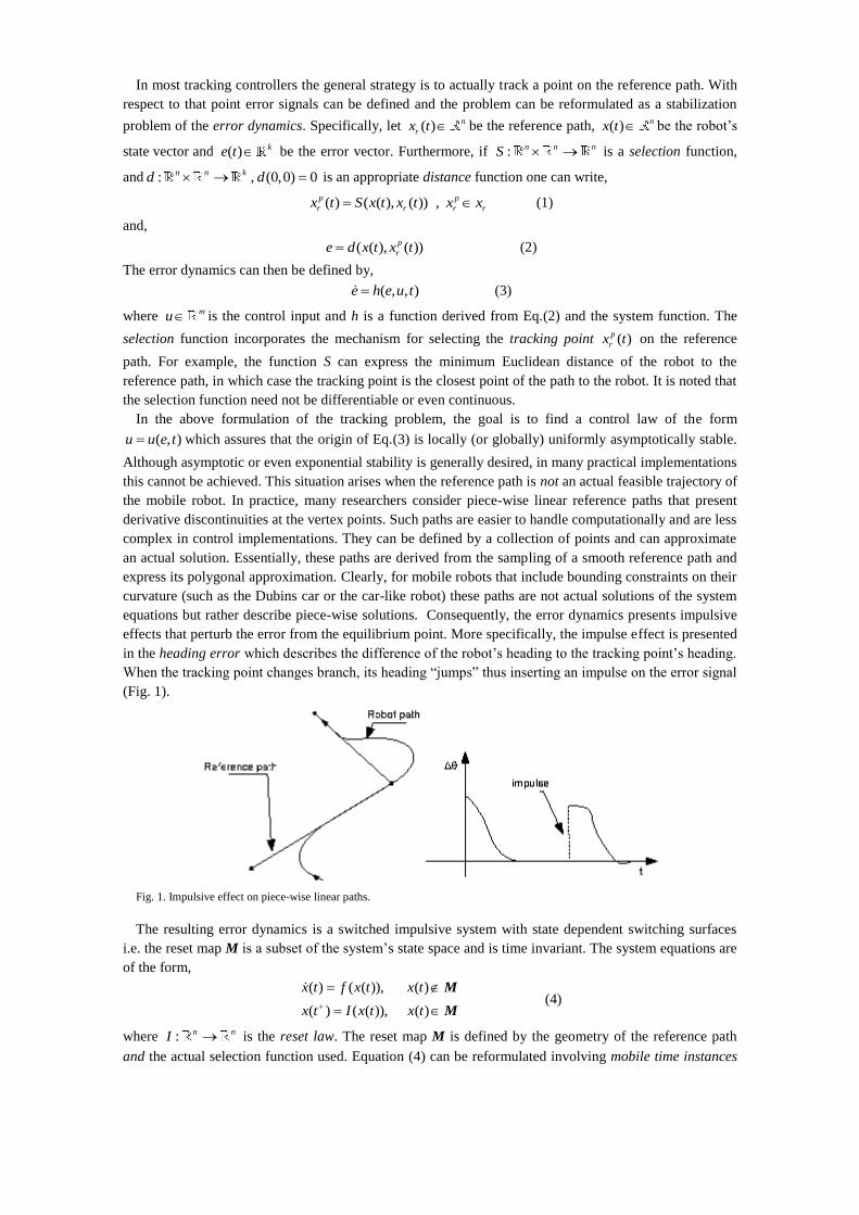
effects that perturb the error from the equilibrium point. More specifically, the impulse effect is presented

in the heading error which describes the difference of the robot’s heading to the tracking point’s heading.

When the tracking point changes branch, its heading “jumps” thus inserting an impulse on the error signal

(Fig. 1).

Fig. 1. Impulsive effect on piece-wise linear paths.

The resulting error dynamics is a switched impulsive system with state dependent switching surfaces

i.e. the reset map M is a subset of the system’s state space and is time invariant. The system equations are

of the form,

( ) ( ( )), ( )

( ) ( ( )), ( )

M

M

x t f x t x t

x t I x t x t (4)

where : n nI is the reset law. The reset map M is defined by the geometry of the reference path

and the actual selection function used. Equation (4) can be reformulated involving mobile time instances

of impulsive jumps. If the system hits the switching surfaces at the time instances i , the discrete set

1 2 1 2{ , .. : ...}E denotes the instances the jumps occur, and Eq. (4) becomes,

( ) ( ( )),

( ) ( ( )), k

x t f x t t E

x t I x t t E

(5)

Notice that the time instances depend on the actual motion of the system i.e. the set E is not

predetermined.

Another repercussion of the introduction of impulsive effects in the tracking control is that, with respect

to the Dubins Car model, the zero set of the error dynamics is not an equilibrium point. An insight of this

behavior can be grasped by inspection of Fig.1. If the system is allowed to perfectly track each edge, thus

driving the error solution to zero, when the robot changes branch the impulse will perturb the heading

error. Thus the origin in not an actual invariant set of the system and consequently cannot be an

equilibrium point (see Shen & Jing, 2006 for some basic definitions on impulsive systems).

Quantitatively this can be deduced from the fact, as will be shown later, that (0) 0f but (0) 0kI .

This paper has a twofold purpose. The first is to present a switching fuzzy tracking controller for the

Dubins Car, tracking polygonal paths. The controller is a Takagi-Sugeno zero-order type FLC with

triangular membership functions and an overlap of two. The tracking control of such paths is rather

important since many tracking applications resort in practice to such path formulations, although the

effect of the polygonization is often overlooked since the error is kept small. The second purpose

however, is the presentation of the actual methodology used that resulted to this controller. Note the word

“resulted”, since the controller has not been designed ab initio but rather is a simplification of an existing

fuzzy tracker which the authors have used in previous experiments (Deliparaschos et al., 2007). The

prime methodology used is the application of the strip-wise affine map.

The Strip-Wise Affine Map is a piece-wise linear homeomorphism that maps a planar polygonal path in

the so-called physical domain (the actual plane where the robot moves) to a straight line in the canonical

domain. In order to impose bijectivity, the path must be a strictly monotone polygonal chain. This

mapping enables the reduction of path tracking to straight line tracking, something that simplifies the

design of tracking controllers for mobile robots. Furthermore, the transformation also preserves the

system equations, meaning that it maps a car-like robot in the physical domain, to a car-like robot in the

canonical domain. This enables one to use existing tracking controllers for path tracking, albeit simplified

ones in order to track straight lines.

The simplification consists of reducing the fuzzy path tracker to a straight line tracking controller, i.e.

tailoring it to tracking only straight lines, in contrast to arbitrary polygonal paths. This is made feasible

due to the very nature of the strip-wise affine map since by design it “straightens” polygonal chains

(piece-wise linear paths).

II. PRELIMINARY CONCEPTS

The model used in this paper for the kinematic analysis and application is the Dubins Car model

described by Eq.(6), which is a widely used model for the control and analysis of mobile robot kinematics

and behaviour.

cos 0

: sin 0

0

x v

y v

v

(6)

Here x, y denote the coordinates of the midpoint of the rear axle, θ the heading of the robot, κ the

steering curvature and v is the robot’s speed. The speed v is considered constant and the robot is

controlled by the curvature κ, which also obeys a bounding constraint of the form,

max (7)

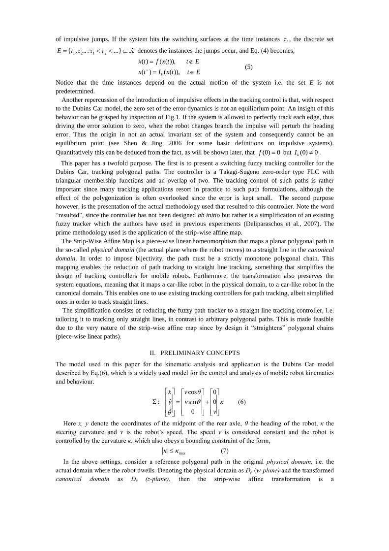
In the above settings, consider a reference polygonal path in the original physical domain, i.e. the

actual domain where the robot dwells. Denoting the physical domain as Dp (w-plane) and the transformed

canonical domain as Dc (z-plane), then the strip-wise affine transformation is a

homeomorphism : c pD D that sends the real line of the canonical domain to the reference polygonal

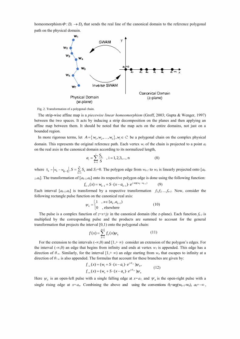
path on the physical domain.

Fig. 2. Transformation of a polygonal chain.

The strip-wise affine map is a piecewise linear homeomorphism (Groff, 2003; Gupta & Wenger, 1997)

between the two spaces. It acts by inducing a strip decomposition on the planes and then applying an

affine map between them. It should be noted that the map acts on the entire domains, not just on a

bounded region.

In more rigorous terms, let 1 2, , , ,n iA w w w w be a polygonal chain on the complex physical

domain. This represents the original reference path. Each vertex wi of the chain is projected to a point ai

on the real axis in the canonical domain according to its normalized length,

1

, i 1,2,3,..., ni

k

i

k

Sa

S

(8)

where 1

,1

n

k k kk

S w wk

S S

and S1=0. The polygon edge from wk-1 to wk is linearly projected onto [ak-

1,ak]. The transformation of [ak-1,ak] onto its respective polygon edge is done using the following function:

1arg( )

1 1 1( ) ( ) k kj w w

k k kf x w S x a e

(9)

Each interval [ak-1,ak] is transformed by a respective transformation f1,f2,…,fn-1. Now, consider the

following rectangle pulse function on the canonical real axis:

11 , [ , )

0 , elsewhere

k k

k

x a a

(10)

The pulse is a complex function of z=x+jy in the canonical domain (the z-plane). Each function fk-1 is

multiplied by the corresponding pulse and the products are summed to account for the general

transformation that projects the interval [0,1) onto the polygonal chain: 1

1

( ) ( )n

k k

k

f x f x

(11)

For the extension to the intervals (-∞,0) and [1,+ ∞) consider an extension of the polygon’s edges. For

the interval (-∞,0) an edge that begins from infinity and ends at vertex w1 is appended. This edge has a

direction of θ-∞. Similarly, for the interval [1,+ ∞) an edge starting from wn that escapes to infinity at a

direction of θ+∞ is also appended. The formulas that account for these branches are given by:

1 1 0( ) ( ( ) ) ,

( ) ( ( ) )

j

j

n n n

f x w S x a e

f x w S x a e

(12)

Here 0 is an open-left pulse with a single falling edge at x=a1, and n is the open-right pulse with a

single rising edge at x=an. Combining the above and using the conventions θk=arg(wk+1-wk), a0= ,

an+1= , 0w the point at infinity corresponding to a0, 1nw

the point at infinity corresponding to an+1,

θ0=arg(w1-w0)= , θ0=arg(wn+1-wn)= , the extended transformation takes the following form:

0

( ) ( ( ) )k

nj

k k k

k

f x w S x a e

(13)

where the functions ,f f correspond to k=0 and k=n respectively. In order to extend this transformation

to the entire complex plane, let z=x+jy be a complex variable in the canonical domain and consider the

following mapping:

( ) ( )sjΦ z y S e f x

(14)

where θs is the shifting angle in [-π/2,π/2]. The complex variable w=u+jv in the physical domain is

identified with the transformation Φ(z),i.e. w=u+jv= Φ(z). This transformation is the direct strip-wise

affine map and produces a linear displacement of the polygon along the direction θs. Each edge of the

polygon produces an affine transformation that applies only in the “strip” that the edge sweeps as it is

being translated. Thus, the transformation Φ(z) can be described as a “strip-wise affine” transformation.

The invertibility of the transformation depends firstly on the geometry of the chain and secondly on the

shifting angle. It can be shown (Moustris & Tzafestas, 2008) that necessary and sufficient conditions for

the mapping to be invertible are that the chain must be a strictly monotone polygonal chain (Preparata &

Supowit, 1981) and that the shifting angle must not coincide with the angle of any of the polyline edges

i.e. the chain must not be shifted along one of its edges.

The inverse strip-wise affine map can be expressed in matrix form by treating Φ(z) as

an 2 to 2 mapping since it cannot be solved analytically with respect to z. The inverse mapping

equations are:

1/

/

kx u C S a

y v C S

(15)

where 0( sin cos / sin( ))

n R I

k k k k s k kkC w w

and A-1 is inverse system matrix, i.e.

1

0

0 0

sin cos

sin(sin cos

/ )

s s n

n ns k k

kk k k k

k k

S

(16)

Besides Eq.(15) one also needs to know the activated pulse since the rectangle pulses are functions of

the variable x, and thus Eq.(15) does not provide a complete solution to the inversion problem. If this

information is provided, the sums in Eq.(15) degenerate and the equation provides the inverse system.

The activated pulse can be calculated algorithmically by doing a point-in-strip test. Consider an axis

orthogonal to the direction θs such that the projection of w1 corresponds to 0. Furthermore consider the

projections of each wi onto that axis, denoted by bi, as well as the projection of the current mapping point,

denoted by bc. The projections of wi apparently partition the axis into consecutive line segments [bi bi+1]

which are into one-to-one correspondence with the edges of the polygonal chain. Then, in order to find

the current pulse one needs to find the segment into which the point bc resides. This can be performed

optimally by a binary search algorithm in O(log n).

III. CONTROL-THEORETIC ANALYSIS

In this section the effect of the map to the system equations of the Dubins Car (Eq.(6)) will be analyzed.

Since the transformation acts on the variables x and y it is clear that the system equations are also

affected. Denoting all the state variables in the physical and canonical domains with a subscript of “p”

and “c” respectively, then the u-v plane (physical domain) is mapped to the x-y plane (canonical domain), i.e.

the state vector [ , , ]T

p p px y x is transformed to [ , , ]T

c c px y x . The homeomorphism Φ defines an

equivalence relation between the two states. Notice that the state θp remains unaffected. By introducing a

new extended homeomorphism Ψ that also maps the heading angle θp, one can send the canonical state-

space to the physical state-space, i.e. ( )x x . This mapping acts on all state variables and the new

system state is [ , , ]T

c c cx y x . This map is defined by,

1 0

0

cos Re( ( ))

sin Im( ( ))( )

sin sin tantan ( )

cos cos tan

c s c

pc s c

np

s c

p n

s c

y S f x

x y S f xy x

(17)

and the new system equations are,

3 3 1

cos 0

: sin 0

0

c cc

c c c p

cc

vx

y v

S J v

(18)

Here J denotes the Jacobian of ( )c cΦ z x jy and 0

1 sin 2 cos( )n

c s

. Notice that the

input p is not affected by the transformation. However, the input of the physical system is also

transformed under since it is the curvature in the physical domain. Thus by including the

transformation of the input and extending the homeomorphism Ψ to ( , ) , where

3 3( , )p c cx S J is the input map that sends the controls from the canonical input space to the

controls in the physical input space, one gets the new extended system ,

cos 0

: sin 0

0

c c c

c c c c

cc

x v

y v

v

(19)

The systems and are said to be feedback-equivalent (Gardner & Shadwick, 1990, 1987). The input

transformation is actually a feedback transformation of that feeds the states x back to the input. Of

course, Eq.(19) expresses the Dubins Car in the canonical domain, thus the map preserves the system

equations. However, if one solves Eq.(17) for θc it can be shown that the heading in the canonical space is

not a continuous function of θp. This is due to the presence of the pulse functionsk .

When the state passes from one pulse to another, the canonical heading jumps impulsively. The

physical heading however is continuous. In the canonical domain the switching surfaces are vertical lines

that pass through the points ai, with one line corresponding to each a. Using standard nomenclature, the

canonical heading just before the jump is denoted by θc and infinitesimally after, by c . When the jump

occurs, the physical heading is the same, thus by Eq.(17) one gets,

1

1

1 1

1

sin sin tan sin sin tan...

cos cos tan cos cos tan

sin( ) tan sin( )tan ( ( ))

sin( )

s c s c

s c s c

c s

c k

s

I t

x

(20)

Eq.(20) describes the reset law of the canonical model. Since the goal of path tracking in the canonical

domain is to track a straight line (the real axis), the error signals are actually the lateral distance from the

real axis, i.e. the coordinate yc , and the heading θc. However Eq.(20) shows that,

1 1

1

sin( )(0) tan

sin( )k

s

I

(21)

thus the impulse at the origin of the error dynamics in not null and perturbs the system away from zero

during the resets. Observe also that the reset amplitude depends on the algebraic value of the state.

Suppose now that one provides a stabilizing feedback law for the continuous dynamics of the error

system (which consists of the subsystem of the two last states of Eq.(19)) that renders the origin

asymptotically stable. Since the input is bounded and controls the derivative of θc, the rate of change of

the heading error is finite. Thus, if the system is at the origin, the input cannot cancel out the impulses at

the reset times; at least, not without affecting the lateral error as well, i.e. the state yc.. In plain terms, there

is no feedback law that can asymptotically stabilize the impulsive system at the origin because no law can

stabilize the continuous dynamics and zero out the impulses at the same time. This is rather expected

since the reference path is not an actual feasible path of the system.

Now, let refp be a reference path in the physical domain (i.e., a strictly monotone polygonal chain on

the w-plane) and let ( , , )c cx I tu be a straight line tracking controller for , where Ic denotes the line

segment { 0 / [0,1]}c cy x of the z-plane, i.e. the reference path in the canonical domain. This controller

is transformed to a path tracking controller up for under Eq.(22), i.e.:

1 1 1( ) )

( )

( ( ) ( )

( , , ) ( , , , )

( , , , )

p ref c

c ref

p t I t

p t

u x u x x

u x x (22)

However, since the system is the Dubins Car in the canonical domain, the straight line tracking

controller ( , , )c x I tu for is actually a straight line tracker for the Dubins Car, and in order to build a

path tracker for the Dubins Car, one has but to build a straight line tracker and use Eq.(22) to promote it

to a path tracker for strictly monotone polygonal chains. Furthermore, one could also use existing path

trackers for the Dubins Car to track the straight line in the canonical domain. In this case, these

controllers can be simplified since in general, straight line tracking is simpler than path tracking.

IV. FUZZY CONTROL

In this application the use and simplification of a fuzzy path tracker developed by the authors, which

has been deployed in previous experiments (Deliparaschos et al., 2007; Moustris, Deliparaschos, &

Tzafestas, 2009; Moustris & Tzafestas, 2005, 2008), is demonstrated. The FL tracker is based on Moustris

& Tzafestas, (2005), along with the modifications presented in Deliparaschos et al., (2007). Specifically

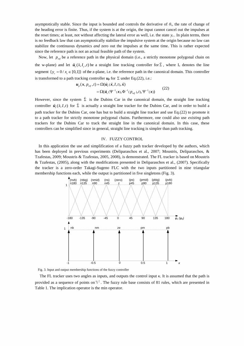
the tracker is a zero-order Takagi-Sugeno FLC with the two inputs partitioned in nine triangular

membership functions each, while the output is partitioned in five singletons (Fig. 3).

φ1 (φ2)

-180 -135 -90 -45 0 45 90 135 180

1n180 n135 n90 n45 z p45 p90 p135 p180(nvb) (nbig) (nmid) (ns) (zero) (ps) (pmid) (pbig) (pvb)

κ

-1 -0.5 0 0.5 1

1 nb nm ze pm pb

Fig. 3. Input and output membership functions of the fuzzy controller

The FL tracker uses two angles as inputs, and outputs the control input κ. It is assumed that the path is

provided as a sequence of points on 2 . The fuzzy rule base consists of 81 rules, which are presented in

Table 1. The implication operator is the min operator.

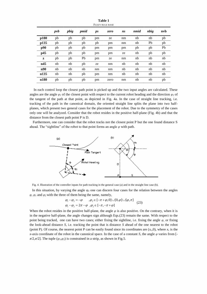
Table 1

FUZZY RULE BASE

pvb pbig pmid ps zero ns nmid nbig nvb

p180 pb pb pb pm ze nm nb nb pb

p135 pb pb pb pb pm nm nb Pb pb

p90 pb pb pb pm pm pm pb pb Pb

p45 pb pb pb pm pm ze nb pb pb

z pb pb Pb pm ze nm nb nb nb

n45 nb nb pb ze nm nb nb nb nb

n90 nb nb nb nm nm nb nb nb nb

n135 nb nb pb pm nm nb nb nb nb

n180 pb pb pb pm zero nm nb nb pb

In each control loop the closest path point is picked up and the two input angles are calculated. These

angles are the angle φ1 of the closest point with respect to the current robot heading and the direction φ2 of

the tangent of the path at that point, as depicted in Fig. 4a. In the case of straight line tracking, i.e.

tracking of the path in the canonical domain, the oriented straight line splits the plane into two half-

planes, which present two general cases for the placement of the robot. Due to the symmetry of the cases

only one will be analyzed. Consider that the robot resides in the positive half-plane (Fig. 4b) and that the

distance from the closest path point P is D.

Furthermore, one can consider that the robot tracks not the closest point P but the one found distance S

ahead. The “sightline” of the robot to that point forms an angle φ with path.

Fig. 4. Illustration of the controller inputs for path tracking in the general case (a) and in the straight line case (b).

In this situation, by varying the angle φ2 one can discern four cases for the relation between the angles

φ, φ1 and φ2 with the three of them being the same, namely,

1 2 2

1 2 2

, [ ,0] [0, ] [ , ]

2 , [ , ]

(23)

When the robot resides in the positive half-plane, the angle φ is also positive. On the contrary, when it is

in the negative half-plane, the angle changes sign although Eqs.(23) remain the same. With respect to the

point being tracked, one can have two cases; either fixing the sightline, i.e. fixing the angle φ, or fixing

the look-ahead distance S, i.e. tracking the point that is distance S ahead of the one nearest to the robot

(point P). Of course, the nearest point P can be easily found since its coordinates are (xc,0), where xc is the

x-axis coordinate of the robot in the canonical space. In the case of a constant S, the angle φ varies from [-

π/2,π/2]. The tuple (φ1,φ2) is constrained in a strip, as shown in Fig.5.

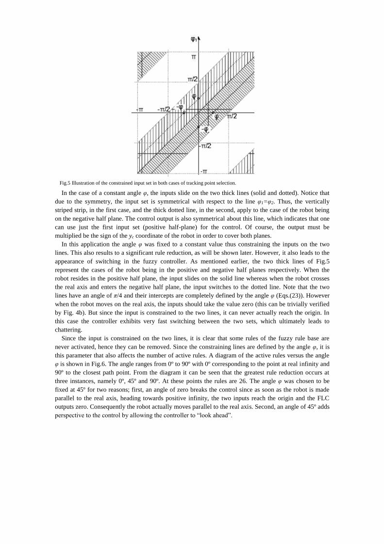
Fig.5 Illustration of the constrained input set in both cases of tracking point selection.

In the case of a constant angle φ, the inputs slide on the two thick lines (solid and dotted). Notice that

due to the symmetry, the input set is symmetrical with respect to the line φ1=φ2. Thus, the vertically

striped strip, in the first case, and the thick dotted line, in the second, apply to the case of the robot being

on the negative half plane. The control output is also symmetrical about this line, which indicates that one

can use just the first input set (positive half-plane) for the control. Of course, the output must be

multiplied be the sign of the yc coordinate of the robot in order to cover both planes.

In this application the angle φ was fixed to a constant value thus constraining the inputs on the two

lines. This also results to a significant rule reduction, as will be shown later. However, it also leads to the

appearance of switching in the fuzzy controller. As mentioned earlier, the two thick lines of Fig.5

represent the cases of the robot being in the positive and negative half planes respectively. When the

robot resides in the positive half plane, the input slides on the solid line whereas when the robot crosses

the real axis and enters the negative half plane, the input switches to the dotted line. Note that the two

lines have an angle of π/4 and their intercepts are completely defined by the angle φ (Eqs.(23)). However

when the robot moves on the real axis, the inputs should take the value zero (this can be trivially verified

by Fig. 4b). But since the input is constrained to the two lines, it can never actually reach the origin. In

this case the controller exhibits very fast switching between the two sets, which ultimately leads to

chattering.

Since the input is constrained on the two lines, it is clear that some rules of the fuzzy rule base are

never activated, hence they can be removed. Since the constraining lines are defined by the angle φ, it is

this parameter that also affects the number of active rules. A diagram of the active rules versus the angle

φ is shown in Fig.6. The angle ranges from 0º to 90º with 0º corresponding to the point at real infinity and

90º to the closest path point. From the diagram it can be seen that the greatest rule reduction occurs at

three instances, namely 0º, 45º and 90º. At these points the rules are 26. The angle φ was chosen to be

fixed at 45º for two reasons; first, an angle of zero breaks the control since as soon as the robot is made

parallel to the real axis, heading towards positive infinity, the two inputs reach the origin and the FLC

outputs zero. Consequently the robot actually moves parallel to the real axis. Second, an angle of 45º adds

perspective to the control by allowing the controller to “look ahead”.

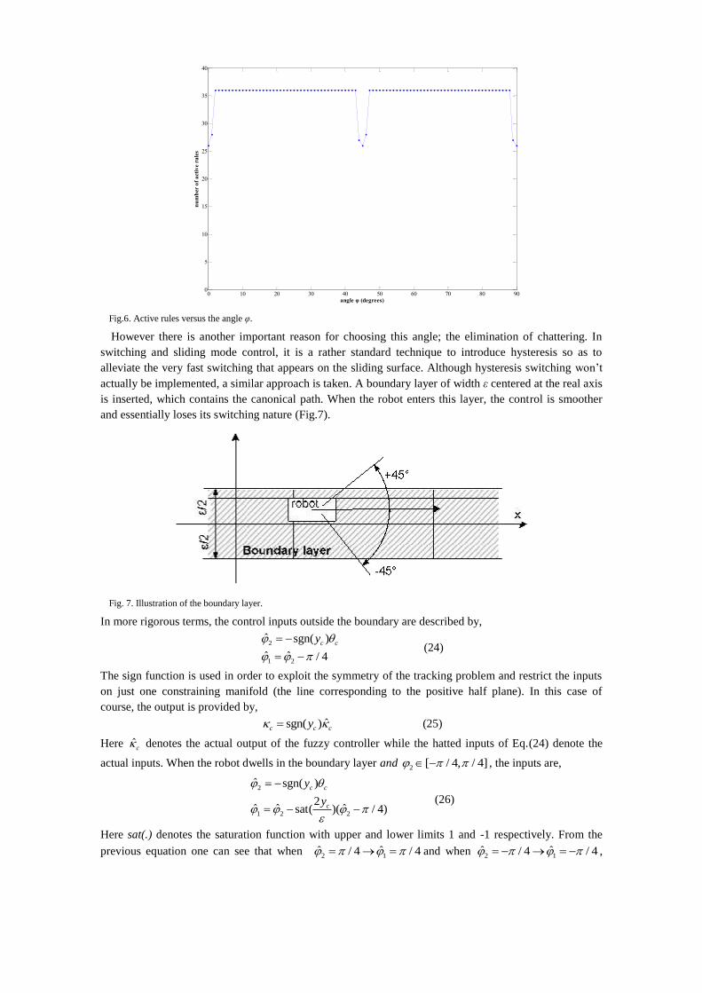
0 10 20 30 40 50 60 70 80 900

5

10

15

20

25

30

35

40

angle φ (degrees)

nu

mb

er o

f a

ctiv

e ru

les

Fig.6. Active rules versus the angle φ.

However there is another important reason for choosing this angle; the elimination of chattering. In

switching and sliding mode control, it is a rather standard technique to introduce hysteresis so as to

alleviate the very fast switching that appears on the sliding surface. Although hysteresis switching won’t

actually be implemented, a similar approach is taken. A boundary layer of width ε centered at the real axis

is inserted, which contains the canonical path. When the robot enters this layer, the control is smoother

and essentially loses its switching nature (Fig.7).

Fig. 7. Illustration of the boundary layer.

In more rigorous terms, the control inputs outside the boundary are described by,

2

1 2

ˆ sgn( )

ˆ ˆ / 4

c cy

(24)

The sign function is used in order to exploit the symmetry of the tracking problem and restrict the inputs

on just one constraining manifold (the line corresponding to the positive half plane). In this case of

course, the output is provided by,

ˆsgn( )c c cy (25)

Here ˆc denotes the actual output of the fuzzy controller while the hatted inputs of Eq.(24) denote the

actual inputs. When the robot dwells in the boundary layer and 2 [ / 4, / 4] , the inputs are,

2

1 2 2

ˆ sgn( )

2ˆ ˆ ˆsat( )( / 4)

c c

c

y

y

(26)

Here sat(.) denotes the saturation function with upper and lower limits 1 and -1 respectively. From the

previous equation one can see that when 2 1ˆ ˆ/ 4 / 4 and when 2 1

ˆ ˆ/ 4 / 4 ,

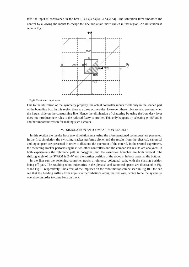
thus the input is constrained in the box [ / 4, / 4] [ / 4, / 4] . The saturation term smoothes the

control by allowing the inputs to escape the line and attain more values in that region. An illustration is

seen in Fig.8.

Fig.8. Constrained input space.

Due to the utilization of the symmetry property, the actual controller inputs dwell only in the shaded part

of the bounding box. In this region there are three active rules. However, these rules are also present when

the inputs slide on the constraining line. Hence the elimination of chattering by using the boundary layer

does not introduce new rules to the reduced fuzzy controller. This only happens by selecting φ=45º and is

another important reason for making such a choice.

V. SIMULATION AND COMPARISON RESULTS

In this section the results from two simulation runs using the aforementioned techniques are presented.

In the first simulation the switching tracker performs alone, and the results from the physical, canonical

and input space are presented in order to illustrate the operation of the control. In the second experiment,

the switching tracker performs against two other controllers and the comparison results are analyzed. In

both experiments the reference path is polygonal and the extension branches are both vertical. The

shifting angle of the SWAM is θs=0º and the starting position of the robot is, in both cases, at the bottom.

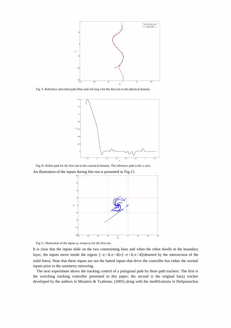
In the first run the switching controller tracks a reference polygonal path, with the starting position

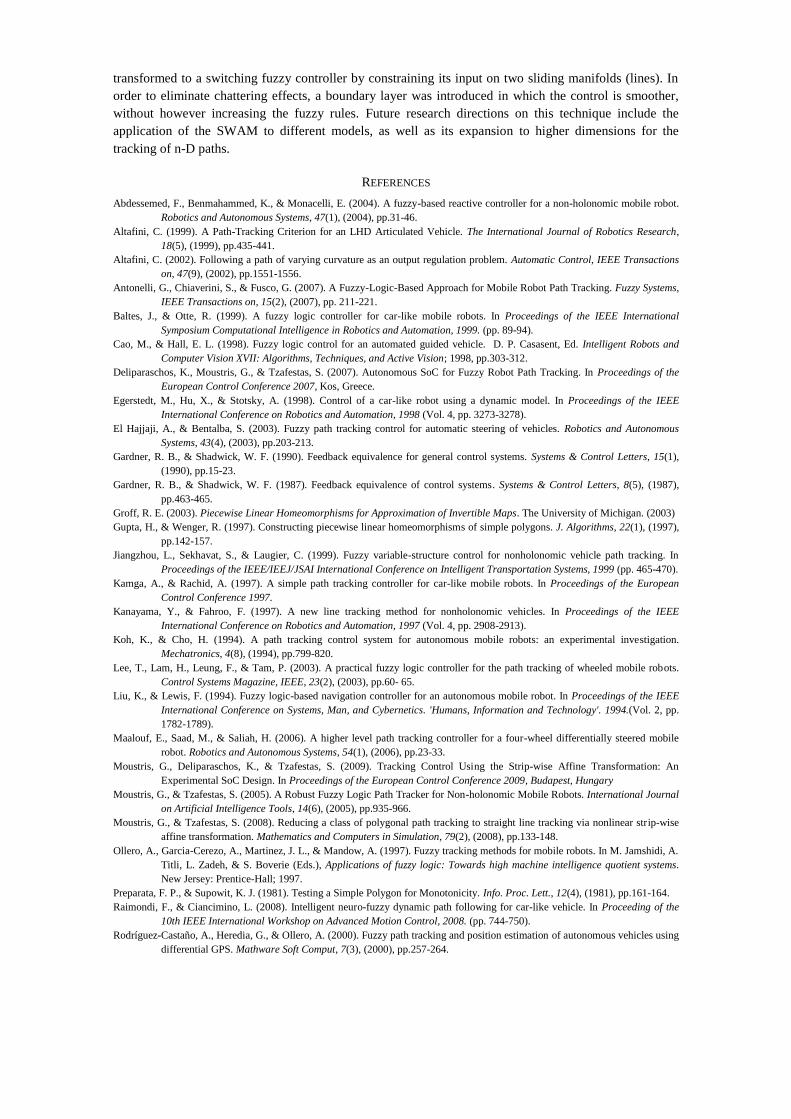
being off-path. The resulting robot trajectories in the physical and canonical spaces are illustrated in Fig.

9 and Fig.10 respectively. The effect of the impulses on the robot motion can be seen in Fig.10. One can

see that the heading suffers from impulsive perturbations along the real axis, which force the system to

overshoot in order to come back on track.

-150 -100 -50 0 50 100

-150

-100

-50

0

50

xp

yp

Reference path

Robot path

Fig. 9. Reference and robot path (blue and red resp.) for the first run in the physical domain.

-0.2 0 0.2 0.4 0.6 0.8 1 1.2

0

0.02

0.04

0.06

0.08

0.1

0.12

0.14

xc

yc

Fig.10. Robot path for the first run in the canonical domain. The reference path is the x-axis.

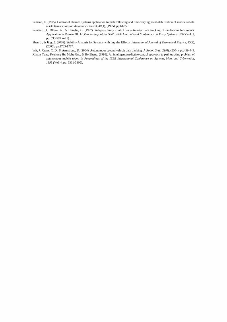
An illustration of the inputs during this run is presented in Fig.11.

-180 -135 -90 -45 0 45 90 135 180-180

-135

-90

-45

0

45

90

135

180

φ2

φ1

Fig.11. Illustration of the inputs φ2 versus φ1 for the first run.

It is clear that the inputs slide on the two constraining lines and when the robot dwells in the boundary

layer, the inputs move inside the region [ / 4, / 4] [ / 4, / 4] (denoted by the intersection of the

solid lines). Note that these inputs are not the hatted inputs that drive the controller but rather the normal

inputs prior to the symmetry mirroring.

The next experiment shows the tracking control of a polygonal path by three path trackers. The first is

the switching tracking controller presented in this paper; the second is the original fuzzy tracker

developed by the authors in Moustris & Tzafestas, (2005) along with the modifications in Deliparaschos

et al.,(2007) and the last is a tracking controller presented in Kamga & Rachid, (1997). In all three cases

the reference path and the starting position is, of course, the same. Fig. 12 shows the results of the three

path trackers in the physical domain.

-60 -40 -20 0 20 40 60 80 100-150

-100

-50

0

50

100

Reference path

Switching tracker

Moustris&Tzafestas 2005

Kamga&Rachid

Fig. 12. Physical paths for the three path trackers.

An analysis of the resulting paths for the three controllers is presented in Table 2.

Table 2

COMPARISON RESULTS FOR THE THREE TRACKING CONTROLLERS

Switching

Tracker

Moustris&Tzafestas

2005 Kamga&Rachid

mean 15.7268 18.0667 17.7592

rms 31.292 32.3431 33.5429

From the analysis it is evident that the switching controller outperforms both trackers. Specifically, the

mean of the distance of the robot path to the reference path is noticeably lower, meaning that the

switching tracker finds the reference path more quickly as well as that it maintains the robot closer to

the reference throughout the tracking control. Second, one can also see that the root-mean-square (rms)

value of the path distance is again lower for the switching tracker. This translates to a smaller variation

of the path distance i.e. the switching controller tracks the path more accurately. Emphasis must be

made on the comparison between the original fuzzy controller and the switching fuzzy controller, since

the later is derived from the former. The results in Table 2 show that the switching tracker performs

significantly better than its predecessor and, combined with the fact that it features 70% fewer rules than

the original fuzzy tracker, it is clear that it presents a vast improvement.

VI. CONCLUSIONS

In this paper the application of the strip-wise affine map to the path tracking problem for wheeled mobile

robots, and especially the Dubins Car, has been presented. This application leads to the “construction” of

a simplified form of a fuzzy controller that has been used in a previous work. The simplification results to

a significantly reduced rule base going from 81 rules to 26 (70% reduction). Furthermore, the controller is

transformed to a switching fuzzy controller by constraining its input on two sliding manifolds (lines). In

order to eliminate chattering effects, a boundary layer was introduced in which the control is smoother,

without however increasing the fuzzy rules. Future research directions on this technique include the

application of the SWAM to different models, as well as its expansion to higher dimensions for the

tracking of n-D paths.

REFERENCES

Abdessemed, F., Benmahammed, K., & Monacelli, E. (2004). A fuzzy-based reactive controller for a non-holonomic mobile robot.

Robotics and Autonomous Systems, 47(1), (2004), pp.31-46.

Altafini, C. (1999). A Path-Tracking Criterion for an LHD Articulated Vehicle. The International Journal of Robotics Research,

18(5), (1999), pp.435-441.

Altafini, C. (2002). Following a path of varying curvature as an output regulation problem. Automatic Control, IEEE Transactions

on, 47(9), (2002), pp.1551-1556.

Antonelli, G., Chiaverini, S., & Fusco, G. (2007). A Fuzzy-Logic-Based Approach for Mobile Robot Path Tracking. Fuzzy Systems,

IEEE Transactions on, 15(2), (2007), pp. 211-221.

Baltes, J., & Otte, R. (1999). A fuzzy logic controller for car-like mobile robots. In Proceedings of the IEEE International

Symposium Computational Intelligence in Robotics and Automation, 1999. (pp. 89-94).

Cao, M., & Hall, E. L. (1998). Fuzzy logic control for an automated guided vehicle. D. P. Casasent, Ed. Intelligent Robots and

Computer Vision XVII: Algorithms, Techniques, and Active Vision; 1998, pp.303-312.

Deliparaschos, K., Moustris, G., & Tzafestas, S. (2007). Autonomous SoC for Fuzzy Robot Path Tracking. In Proceedings of the

European Control Conference 2007, Kos, Greece.

Egerstedt, M., Hu, X., & Stotsky, A. (1998). Control of a car-like robot using a dynamic model. In Proceedings of the IEEE

International Conference on Robotics and Automation, 1998 (Vol. 4, pp. 3273-3278).

El Hajjaji, A., & Bentalba, S. (2003). Fuzzy path tracking control for automatic steering of vehicles. Robotics and Autonomous

Systems, 43(4), (2003), pp.203-213.

Gardner, R. B., & Shadwick, W. F. (1990). Feedback equivalence for general control systems. Systems & Control Letters, 15(1),

(1990), pp.15-23.

Gardner, R. B., & Shadwick, W. F. (1987). Feedback equivalence of control systems. Systems & Control Letters, 8(5), (1987),

pp.463-465.

Groff, R. E. (2003). Piecewise Linear Homeomorphisms for Approximation of Invertible Maps. The University of Michigan. (2003)

Gupta, H., & Wenger, R. (1997). Constructing piecewise linear homeomorphisms of simple polygons. J. Algorithms, 22(1), (1997),

pp.142-157.

Jiangzhou, L., Sekhavat, S., & Laugier, C. (1999). Fuzzy variable-structure control for nonholonomic vehicle path tracking. In

Proceedings of the IEEE/IEEJ/JSAI International Conference on Intelligent Transportation Systems, 1999 (pp. 465-470).

Kamga, A., & Rachid, A. (1997). A simple path tracking controller for car-like mobile robots. In Proceedings of the European

Control Conference 1997.

Kanayama, Y., & Fahroo, F. (1997). A new line tracking method for nonholonomic vehicles. In Proceedings of the IEEE

International Conference on Robotics and Automation, 1997 (Vol. 4, pp. 2908-2913).

Koh, K., & Cho, H. (1994). A path tracking control system for autonomous mobile robots: an experimental investigation.

Mechatronics, 4(8), (1994), pp.799-820.

Lee, T., Lam, H., Leung, F., & Tam, P. (2003). A practical fuzzy logic controller for the path tracking of wheeled mobile robots.

Control Systems Magazine, IEEE, 23(2), (2003), pp.60- 65.

Liu, K., & Lewis, F. (1994). Fuzzy logic-based navigation controller for an autonomous mobile robot. In Proceedings of the IEEE

International Conference on Systems, Man, and Cybernetics. 'Humans, Information and Technology'. 1994.(Vol. 2, pp.

1782-1789).

Maalouf, E., Saad, M., & Saliah, H. (2006). A higher level path tracking controller for a four-wheel differentially steered mobile

robot. Robotics and Autonomous Systems, 54(1), (2006), pp.23-33.

Moustris, G., Deliparaschos, K., & Tzafestas, S. (2009). Tracking Control Using the Strip-wise Affine Transformation: An

Experimental SoC Design. In Proceedings of the European Control Conference 2009, Budapest, Hungary

Moustris, G., & Tzafestas, S. (2005). A Robust Fuzzy Logic Path Tracker for Non-holonomic Mobile Robots. International Journal

on Artificial Intelligence Tools, 14(6), (2005), pp.935-966.

Moustris, G., & Tzafestas, S. (2008). Reducing a class of polygonal path tracking to straight line tracking via nonlinear strip-wise

affine transformation. Mathematics and Computers in Simulation, 79(2), (2008), pp.133-148.

Ollero, A., Garcia-Cerezo, A., Martinez, J. L., & Mandow, A. (1997). Fuzzy tracking methods for mobile robots. In M. Jamshidi, A.

Titli, L. Zadeh, & S. Boverie (Eds.), Applications of fuzzy logic: Towards high machine intelligence quotient systems.

New Jersey: Prentice-Hall; 1997.

Preparata, F. P., & Supowit, K. J. (1981). Testing a Simple Polygon for Monotonicity. Info. Proc. Lett., 12(4), (1981), pp.161-164.

Raimondi, F., & Ciancimino, L. (2008). Intelligent neuro-fuzzy dynamic path following for car-like vehicle. In Proceeding of the

10th IEEE International Workshop on Advanced Motion Control, 2008. (pp. 744-750).

Rodríguez-Castaño, A., Heredia, G., & Ollero, A. (2000). Fuzzy path tracking and position estimation of autonomous vehicles using

differential GPS. Mathware Soft Comput, 7(3), (2000), pp.257-264.

Samson, C. (1995). Control of chained systems application to path following and time-varying point-stabilization of mobile robots.

IEEE Transactions on Automatic Control, 40(1), (1995), pp.64-77.

Sanchez, O., Ollero, A., & Heredia, G. (1997). Adaptive fuzzy control for automatic path tracking of outdoor mobile robots.

Application to Romeo 3R. In. Proceedings of the Sixth IEEE International Conference on Fuzzy Systems, 1997 (Vol. 1,

pp. 593-599 vol.1).

Shen, J., & Jing, Z. (2006). Stability Analysis for Systems with Impulse Effects. International Journal of Theoretical Physics, 45(9),

(2006), pp.1703-1717.

Wit, J., Crane, C. D., & Armstrong, D. (2004). Autonomous ground vehicle path tracking. J. Robot. Syst., 21(8), (2004), pp.439-449.

Xinxin Yang, Kezhong He, Muhe Guo, & Bo Zhang. (1998). An intelligent predictive control approach to path tracking problem of

autonomous mobile robot. In Proceedings of the IEEE International Conference on Systems, Man, and Cybernetics,

1998 (Vol. 4, pp. 3301-3306).