Switch of Sensitivity Dynamics Revealed with DyGloSA Toolbox for Dynamical Global Sensitivity Analysis as an Early Warning for System's Critical Transition

Switch of Sensitivity Dynamics Revealed with DyGloSAToolbox for Dynamical Global Sensitivity Analysis as anEarly Warning for System’s Critical TransitionTatiana Baumuratova1,2*, Simona Dobre3, Thierry Bastogne4,5,6, Thomas Sauter1

1 Systems Biology Group, Life Sciences Research Unit, University of Luxembourg, Luxembourg, Luxembourg, 2 Institute of Mathematical Problems of Biology, Russian

Academy of Sciences, Pushchino, Moscow Region, Russia, 3 ISL, French-German Research Institute of Saint-Louis, Saint-Louis, France, 4 Universite de Lorraine, CRAN, UMR

7039, Vandœuvre-les-Nancy, France, 5 CNRS, CRAN, UMR 7039, Vandœuvre-les-Nancy, France, 6 INRIA, BIGS, Vandœuvre-les-Nancy, France

Abstract

Systems with bifurcations may experience abrupt irreversible and often unwanted shifts in their performance, called criticaltransitions. For many systems like climate, economy, ecosystems it is highly desirable to identify indicators serving as earlywarnings of such regime shifts. Several statistical measures were recently proposed as early warnings of critical transitionsincluding increased variance, autocorrelation and skewness of experimental or model-generated data. The lack ofautomatized tool for model-based prediction of critical transitions led to designing DyGloSA – a MATLAB toolbox fordynamical global parameter sensitivity analysis (GPSA) of ordinary differential equations models. We suggest that the switchin dynamics of parameter sensitivities revealed by our toolbox is an early warning that a system is approaching a criticaltransition. We illustrate the efficiency of our toolbox by analyzing several models with bifurcations and predicting the timeperiods when systems can still avoid going to a critical transition by manipulating certain parameter values, which is notdetectable with the existing SA techniques. DyGloSA is based on the SBToolbox2 and contains functions, which computedynamically the global sensitivity indices of the system by applying four main GPSA methods: eFAST, Sobol’s ANOVA, PRCCand WALS. It includes parallelized versions of the functions enabling significant reduction of the computational time (up to12 times). DyGloSA is freely available as a set of MATLAB scripts at http://bio.uni.lu/systems_biology/software/dyglosa. Itrequires installation of MATLAB (versions R2008b or later) and the Systems Biology Toolbox2 available at www.sbtoolbox2.org. DyGloSA can be run on Windows and Linux systems, -32 and -64 bits.

Citation: Baumuratova T, Dobre S, Bastogne T, Sauter T (2013) Switch of Sensitivity Dynamics Revealed with DyGloSA Toolbox for Dynamical Global SensitivityAnalysis as an Early Warning for System’s Critical Transition. PLoS ONE 8(12): e82973. doi:10.1371/journal.pone.0082973

Editor: Gennady Cymbalyuk, Georgia State University, United States of America

Received February 4, 2013; Accepted November 4, 2013; Published December 18, 2013

Copyright: � 2013 Baumuratova et al. This is an open-access article distributed under the terms of the Creative Commons Attribution License, which permitsunrestricted use, distribution, and reproduction in any medium, provided the original author and source are credited.

Funding: The work was supported by the University of Luxembourg. The funders had no role in study design, data collection and analysis, decision to publish, orpreparation of the manuscript.

Competing Interests: The authors have declared that no competing interests exist.

* E-mail: [email protected]

Introduction

Recently the topic of system’s critical transitions, or so-called

tipping points, where a complex system performs a steep

irreversible shift from one state to another, is getting an increasing

attention [1–12]. Many systems in different domains of science are

known to experience such abrupt shifts, like those in economics

and global finance [13,14], sociology [15], ecology and climate

research [1,6,16], human physiology and medicine [17–19].

Recent theory suggests that critical transitions occur when a

system passes its stability threshold [2,9,11]. While approaching

the tipping point the system very slowly recovers from perturba-

tions [2] and this effect is known in dynamical systems theory as

‘critical slowing down’ (CSD) [20,21].

There were a number of studies targeting quantification of CSD

and early prediction of the tipping points. Due to a limited

capacities of modeling systems like climate or large ecosystems,

model-based approaches for predicting the tipping points in such

systems were considered dispensable [22] and the priority was

given to data-driven approaches for quantifying the CSD by

analyzing both model-generated and experimental time series

data. Among possible measures of indication of system’s irrevers-

ible change, there were proposed degenerate fingerprinting

[21,23], changes in spectral properties [24], increased autocorre-

lation [21,22,25] and variance [3,19,25]. These are attempts to

find an alternative to a natural test for system’s CSD which would

be the study of how a system recovers from small experimental

perturbations [22]. Although successful efforts were made recently

to find experimentally early warnings of CSD using this approach

[4], for some systems it might be irrelevant because of the difficulty

to perform such experiments or when analyzing events happened

in the past. In this context, model-based prediction of CSDs

becomes more attractive. Examples of such predictions are shown

in [10,21,22,26]. However when favoring model-based methods of

CSD prediction one should consider the non-linearity of the

system structure and uncertainty of its parameter values which

might seriously affect the resulting predictions.

In this paper we demonstrate the use of a widely known

technique, parameter sensitivity analysis (PSA), to give early

warnings of critical transitions of systems with bifurcations. PSA

apportions the uncertainty in the model output to different sources

of uncertainty in the model parameters which are characterized by

large variation intervals. Local and global PSA methods are

PLOS ONE | www.plosone.org 1 December 2013 | Volume 8 | Issue 12 | e82973

distinguished, where local ones study the effect of a single

parameter variation (in the close vicinity to its nominal value) on

the variation of a model output and global PSA shows how the

overall variability of the model output can be associated with the

variations of model parameters (considering the whole parameter

state space (PSS)).

The MATLAB toolbox DyGloSA presented here allows the

computation of dynamical global sensitivity indices (DGSIs) of

ordinary differential equations (ODE) models and proposes that

the switches in DGSIs behavior are early warnings of system’s

critical transitions. So far the usage of PSA methods for model-

based predictions of CSD was very limited [21], in our opinion,

because there were no automatized tool for performing dynamical

global PSA. Various MATLAB toolboxes, like SBtoolbox2 [27]

and SensSB [28], provide either the output of a single value of

global sensitivity indices (GSIs) calculated for the given time

interval [29–32], or dynamical, but local sensitivity indices (LSIs).

However, neither dynamical LSIs nor snapshots of GSIs are

capable to identify that a system approaches the critical transition:

first ones provide a linear analysis of sensitivity dynamics and may

be inappropriate for complex non-linear systems; the second ones

provide only the state of sensitivity pattern at the end of the time

interval and are not informative in terms of revealing the dynamics

of sensitivity changes. Nevertheless, global dynamics is the

underlying feature of all biological processes at all levels, and

GSIs of biological models are also dynamically changing.

Although some studies concerned the evaluation of GSIs over

time [33–35], the lack of a convenient tool for computing

dynamical GSIs reasoned developing of the DyGloSA toolbox. We

suggest that the switch in dynamics of parameter sensitivities

revealed by our toolbox provides the early warning that a system is

approaching its critical transition. We demonstrate the efficiency

of our toolbox by analyzing several models with multiple stability

and predicting the time periods when systems can still avoid going

to a critical transition by manipulating with certain parameter

values.

Results and Discussion

Overview of the design and implementation of DyGloSAtoolbox

DyGloSA is a MATLAB toolbox allowing the computation of

dynamical GSIs of ODE models employing four GPSA methods

[33]: two variance-based methods, namely Sobol’s analysis of

variance (ANOVA) [36,37] and extended Fourrier amplitude

sensitivity test (eFAST) [38]; partial rank correlation coefficients

(PRCC) [39] and weighted average of local sensitivities (WALS)

[40]. It is based on the respective functions for GPSA implemented

in SB Toolbox2. For each of these GPSA methods DyGloSA

includes a corresponding function for the computation of GSIs for

parameters of the studied ODE model at each time step of the

given time interval. Therefore the main input for DyGloSA

functions is the ODE model given in SBML format. We briefly

describe some additional inputs below, and the full description of

the functions is included in the downloadable archive along with

the toolbox and some examples. Outputs of the dynamical GPSA

functions include the 3-D table of SIs of size (number of

parameters)-by-(number of model states)-by-(time instances). In

the downloadable archive we provide a sample program of how

the SIs can be visualized and further in the Results section we

explain how to analyze the obtained sensitivity profiles to examine

the model behavior and find optimal times of adapting the

system’s performance in a desirable manner.

Parallelized computationAs biological models are usually stiff and large, and accurate

estimation of the numerical solutions require large number of

sampling points of the PSS, the computation of SIs can be time

consuming (from several hours to several days, depending on the

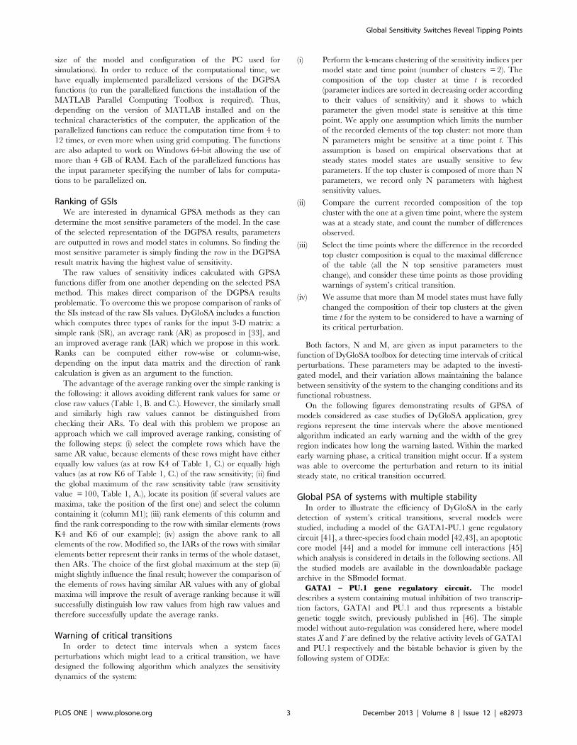
Table 1. Different ranking of the sample table of sensitivity indices.

A. Sensitivity values (raw) B. Simple ranks (SR)

M1 M2 M3 M4 M1 M2 M3 M4

K1 100 45 99 10 K1 4 2 3 1

K2 100 55 20 30 K2 4 3 1 2

K3 98 34 45 100 K3 3 1 2 4

K4 85 85 79 82 K4 3 4 1 2

K5 50 30 20 47 K5 4 2 1 3

K6 0 0 0 0 K6 1 2 3 4

C. Average ranks (AR) D. Improved average ranks (IAR)

M1 M2 M3 M4 M1 M2 M3 M4

K1 3.5 2 3.5 1 K1 3.5 2 3.5 1

K2 3.5 3 1.5 2 K2 3.5 3 1.5 2

K3 3.5 1.5 1.5 3.5 K3 3.5 1.5 1.5 3.5

K4 2.5 2.5 2.5 2.5 K4 3 3 3 3

K5 3 2.5 1.5 3 K5 3 2.5 1.5 3

K6 2.5 2.5 2.5 2.5 K6 1 1 1 1

Model states are located in columns (M1 to M4), parameters are located in rows (K1 to K6). A. Sample raw values of SIs; B. simple ranks (SR) of A - direct indication ofsensitive parameters (rows) is not feasible; C. average ranks (AR) of A – parameters K4 and K6 seem to have similar sensitivity, however K4 is highly sensitive (accordingto raw values from A), and K6 is not sensitive at all; D. improved average ranks (IAR) of A – here the K4 is shown to be sensitive, and K6 is insensitive.doi:10.1371/journal.pone.0082973.t001

Global Sensitivity Switches Reveal Tipping Points


size of the model and configuration of the PC used for

simulations). In order to reduce of the computational time, we

have equally implemented parallelized versions of the DGPSA

functions (to run the parallelized functions the installation of the

MATLAB Parallel Computing Toolbox is required). Thus,

depending on the version of MATLAB installed and on the

technical characteristics of the computer, the application of the

parallelized functions can reduce the computation time from 4 to

12 times, or even more when using grid computing. The functions

are also adapted to work on Windows 64-bit allowing the use of

more than 4 GB of RAM. Each of the parallelized functions has

the input parameter specifying the number of labs for computa-

tions to be parallelized on.

Ranking of GSIsWe are interested in dynamical GPSA methods as they can

determine the most sensitive parameters of the model. In the case

of the selected representation of the DGPSA results, parameters

are outputted in rows and model states in columns. So finding the

most sensitive parameter is simply finding the row in the DGPSA

result matrix having the highest value of sensitivity.

The raw values of sensitivity indices calculated with GPSA

functions differ from one another depending on the selected PSA

method. This makes direct comparison of the DGPSA results

problematic. To overcome this we propose comparison of ranks of

the SIs instead of the raw SIs values. DyGloSA includes a function

which computes three types of ranks for the input 3-D matrix: a

simple rank (SR), an average rank (AR) as proposed in [33], and

an improved average rank (IAR) which we propose in this work.

Ranks can be computed either row-wise or column-wise,

depending on the input data matrix and the direction of rank

calculation is given as an argument to the function.

The advantage of the average ranking over the simple ranking is

the following: it allows avoiding different rank values for same or

close raw values (Table 1, B. and C.). However, the similarly small

and similarly high raw values cannot be distinguished from

checking their ARs. To deal with this problem we propose an

approach which we call improved average ranking, consisting of

the following steps: (i) select the complete rows which have the

same AR value, because elements of these rows might have either

equally low values (as at row K4 of Table 1, C.) or equally high

values (as at row K6 of Table 1, C.) of the raw sensitivity; (ii) find

the global maximum of the raw sensitivity table (raw sensitivity

value = 100, Table 1, A.), locate its position (if several values are

maxima, take the position of the first one) and select the column

containing it (column M1); (iii) rank elements of this column and

find the rank corresponding to the row with similar elements (rows

K4 and K6 of our example); (iv) assign the above rank to all

elements of the row. Modified so, the IARs of the rows with similar

elements better represent their ranks in terms of the whole dataset,

then ARs. The choice of the first global maximum at the step (ii)

might slightly influence the final result; however the comparison of

the elements of rows having similar AR values with any of global

maxima will improve the result of average ranking because it will

successfully distinguish low raw values from high raw values and

therefore successfully update the average ranks.

Warning of critical transitionsIn order to detect time intervals when a system faces

perturbations which might lead to a critical transition, we have

designed the following algorithm which analyzes the sensitivity

dynamics of the system:

(i) Perform the k-means clustering of the sensitivity indices per

model state and time point (number of clusters = 2). The

composition of the top cluster at time t is recorded

(parameter indices are sorted in decreasing order according

to their values of sensitivity) and it shows to which

parameter the given model state is sensitive at this time

point. We apply one assumption which limits the number

of the recorded elements of the top cluster: not more than

N parameters might be sensitive at a time point t. This

assumption is based on empirical observations that at

steady states model states are usually sensitive to few

parameters. If the top cluster is composed of more than N

parameters, we record only N parameters with highest

sensitivity values.

(ii) Compare the current recorded composition of the top

cluster with the one at a given time point, where the system

was at a steady state, and count the number of differences

observed.

(iii) Select the time points where the difference in the recorded

top cluster composition is equal to the maximal difference

of the table (all the N top sensitive parameters must

change), and consider these time points as those providing

warnings of system’s critical transition.

(iv) We assume that more than M model states must have fully

changed the composition of their top clusters at the given

time t for the system to be considered to have a warning of

its critical perturbation.

Both factors, N and M, are given as input parameters to the

function of DyGloSA toolbox for detecting time intervals of critical

perturbations. These parameters may be adapted to the investi-

gated model, and their variation allows maintaining the balance

between sensitivity of the system to the changing conditions and its

functional robustness.

On the following figures demonstrating results of GPSA of

models considered as case studies of DyGloSA application, grey

regions represent the time intervals where the above mentioned

algorithm indicated an early warning and the width of the grey

region indicates how long the warning lasted. Within the marked

early warning phase, a critical transition might occur. If a system

was able to overcome the perturbation and return to its initial

steady state, no critical transition occurred.

Global PSA of systems with multiple stabilityIn order to illustrate the efficiency of DyGloSA in the early

detection of system’s critical transitions, several models were

studied, including a model of the GATA1-PU.1 gene regulatory

circuit [41], a three-species food chain model [42,43], an apoptotic

core model [44] and a model for immune cell interactions [45]

which analysis is considered in details in the following sections. All

the studied models are available in the downloadable package

archive in the SBmodel format.

GATA1 – PU.1 gene regulatory circuit. The model

describes a system containing mutual inhibition of two transcrip-

tion factors, GATA1 and PU.1 and thus represents a bistable

genetic toggle switch, previously published in [46]. The simple

model without auto-regulation was considered here, where model

states X and Y are defined by the relative activity levels of GATA1

and PU.1 respectively and the bistable behavior is given by the

following system of ODEs:



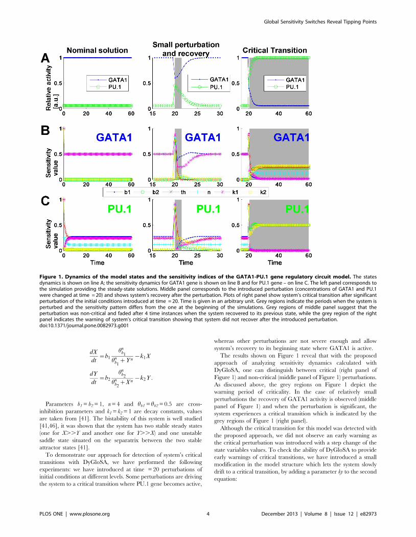
dX

dt~b1

hnb1

hnb1

zY n{k1X

dY

dt~b2

hnb2

hnb2

zX n{k2Y :

Parameters b1 = b2 = 1, n = 4 and hb1 = hb2 = 0.5 are cross-

inhibition parameters and k1 = k2 = 1 are decay constants, values

are taken from [41]. The bistability of this system is well studied

[41,46], it was shown that the system has two stable steady states

(one for X..Y and another one for Y..X) and one unstable

saddle state situated on the separatrix between the two stable

attractor states [41].

To demonstrate our approach for detection of system’s critical

transitions with DyGloSA, we have performed the following

experiments: we have introduced at time = 20 perturbations of

initial conditions at different levels. Some perturbations are driving

the system to a critical transition where PU.1 gene becomes active,

whereas other perturbations are not severe enough and allow

system’s recovery to its beginning state where GATA1 is active.

The results shown on Figure 1 reveal that with the proposed

approach of analyzing sensitivity dynamics calculated with

DyGloSA, one can distinguish between critical (right panel of

Figure 1) and non-critical (middle panel of Figure 1) perturbations.

As discussed above, the grey regions on Figure 1 depict the

warning period of criticality. In the case of relatively small

perturbations the recovery of GATA1 activity is observed (middle

panel of Figure 1) and when the perturbation is significant, the

system experiences a critical transition which is indicated by the

grey regions of Figure 1 (right panel).

Although the critical transition for this model was detected with

the proposed approach, we did not observe an early warning as

the critical perturbation was introduced with a step change of the

state variables values. To check the ability of DyGloSA to provide

early warnings of critical transitions, we have introduced a small

modification in the model structure which lets the system slowly

drift to a critical transition, by adding a parameter ky to the second

equation:

Figure 1. Dynamics of the model states and the sensitivity indices of the GATA1-PU.1 gene regulatory circuit model. The statesdynamics is shown on line A; the sensitivity dynamics for GATA1 gene is shown on line B and for PU.1 gene – on line C. The left panel corresponds tothe simulation providing the steady-state solutions. Middle panel corresponds to the introduced perturbation (concentrations of GATA1 and PU.1were changed at time = 20) and shows system’s recovery after the perturbation. Plots of right panel show system’s critical transition after significantperturbation of the initial conditions introduced at time = 20. Time is given in an arbitrary unit. Grey regions indicate the periods when the system isperturbed and the sensitivity pattern differs from the one at the beginning of the simulations. Grey regions of middle panel suggest that theperturbation was non-critical and faded after 4 time instances when the system recovered to its previous state, while the grey region of the rightpanel indicates the warning of system’s critical transition showing that system did not recover after the introduced perturbation.doi:10.1371/journal.pone.0082973.g001



dX

dt~b1

hnb1

hnb1

zY n{k1X

dY

dt~b2

hnb2

hnb2

zX n{k2Yzky

The addition of the parameter has no influence on the system’s

bistability pattern when its value is low (up to ,0.15), and it causes

the inactivation of the first steady state (X..Y) when ky is higher

than ,0.2. The modified system was perturbed by increasing at

time = 20 the parameter ky to non-critical or to critical values

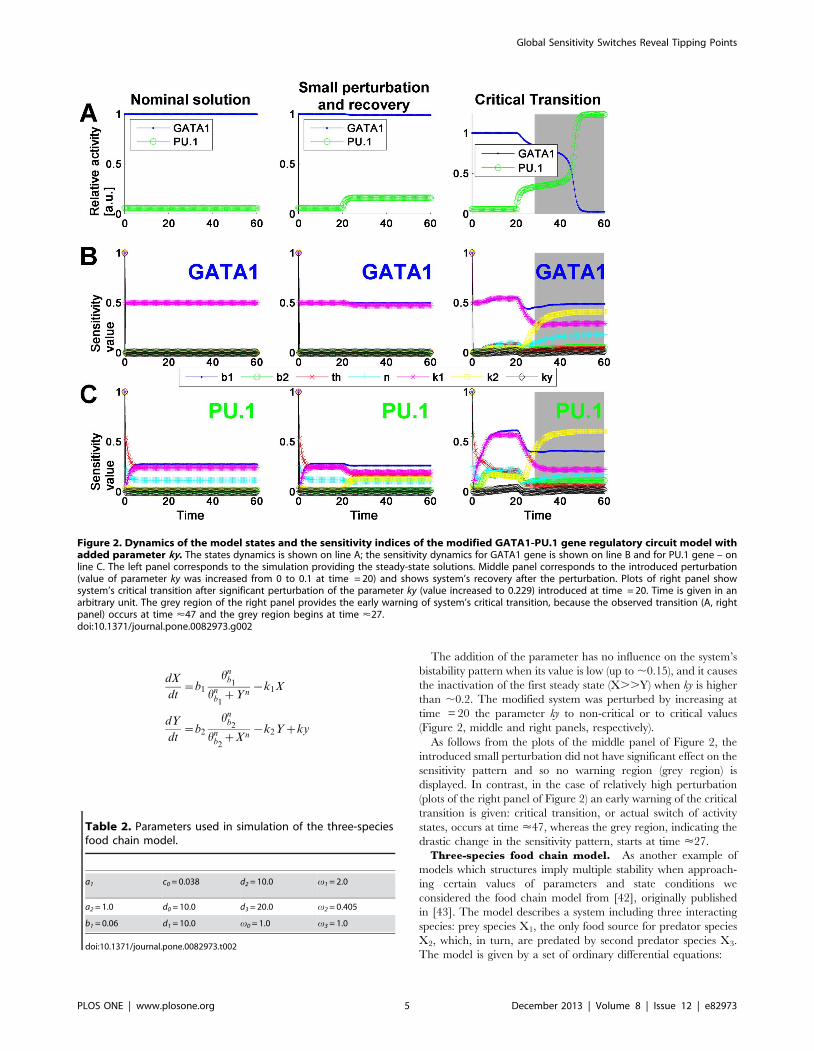
(Figure 2, middle and right panels, respectively).

As follows from the plots of the middle panel of Figure 2, the

introduced small perturbation did not have significant effect on the

sensitivity pattern and so no warning region (grey region) is

displayed. In contrast, in the case of relatively high perturbation

(plots of the right panel of Figure 2) an early warning of the critical

transition is given: critical transition, or actual switch of activity

states, occurs at time <47, whereas the grey region, indicating the

drastic change in the sensitivity pattern, starts at time <27.

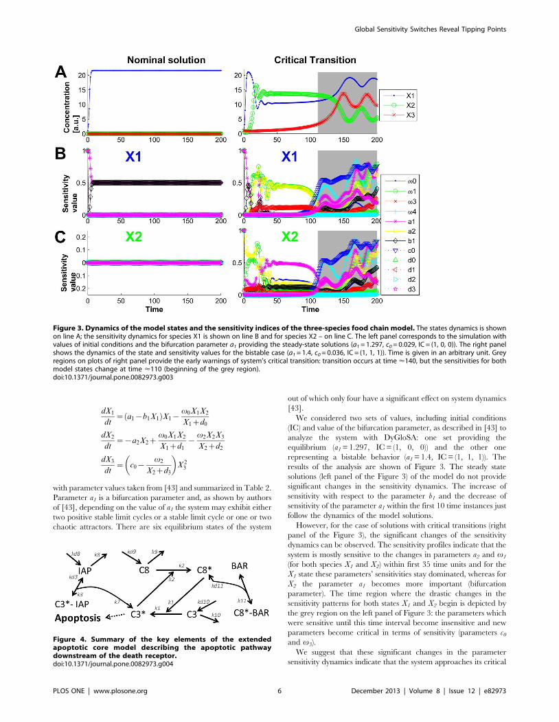
Three-species food chain model. As another example of

models which structures imply multiple stability when approach-

ing certain values of parameters and state conditions we

considered the food chain model from [42], originally published

in [43]. The model describes a system including three interacting

species: prey species X1, the only food source for predator species

X2, which, in turn, are predated by second predator species X3.

The model is given by a set of ordinary differential equations:

Figure 2. Dynamics of the model states and the sensitivity indices of the modified GATA1-PU.1 gene regulatory circuit model withadded parameter ky. The states dynamics is shown on line A; the sensitivity dynamics for GATA1 gene is shown on line B and for PU.1 gene – online C. The left panel corresponds to the simulation providing the steady-state solutions. Middle panel corresponds to the introduced perturbation(value of parameter ky was increased from 0 to 0.1 at time = 20) and shows system’s recovery after the perturbation. Plots of right panel showsystem’s critical transition after significant perturbation of the parameter ky (value increased to 0.229) introduced at time = 20. Time is given in anarbitrary unit. The grey region of the right panel provides the early warning of system’s critical transition, because the observed transition (A, rightpanel) occurs at time <47 and the grey region begins at time <27.doi:10.1371/journal.pone.0082973.g002

Table 2. Parameters used in simulation of the three-speciesfood chain model.

a1 c0 = 0.038 d2 = 10.0 v1 = 2.0

a2 = 1.0 d0 = 10.0 d3 = 20.0 v2 = 0.405

b1 = 0.06 d1 = 10.0 v0 = 1.0 v3 = 1.0

doi:10.1371/journal.pone.0082973.t002



dX1

dt~ a1{b1X1ð ÞX1{

v0X1X2

X1zd0

dX2

dt~{a2X2z

v0X1X2

X1zd1{

v2X2X3

X2zd2

dX3

dt~ c0{

v2

X2zd3

� �X 2

3

with parameter values taken from [43] and summarized in Table 2.

Parameter a1 is a bifurcation parameter and, as shown by authors

of [43], depending on the value of a1 the system may exhibit either

two positive stable limit cycles or a stable limit cycle or one or two

chaotic attractors. There are six equilibrium states of the system

out of which only four have a significant effect on system dynamics

[43].

We considered two sets of values, including initial conditions

(IC) and value of the bifurcation parameter, as described in [43] to

analyze the system with DyGloSA: one set providing the

equilibrium (a1 = 1.297, IC = (1, 0, 0)) and the other one

representing a bistable behavior (a1 = 1.4, IC = (1, 1, 1)). The

results of the analysis are shown of Figure 3. The steady state

solutions (left panel of the Figure 3) of the model do not provide

significant changes in the sensitivity dynamics. The increase of

sensitivity with respect to the parameter b1 and the decrease of

sensitivity of the parameter a1 within the first 10 time instances just

follow the dynamics of the model solutions.

However, for the case of solutions with critical transitions (right

panel of the Figure 3), the significant changes of the sensitivity

dynamics can be observed. The sensitivity profiles indicate that the

system is mostly sensitive to the changes in parameters a2 and v1

(for both species X1 and X2) within first 35 time units and for the

X1 state these parameters’ sensitivities stay dominated, whereas for

X2 the parameter a1 becomes more important (bifurcation

parameter). The time region where the drastic changes in the

sensitivity patterns for both states X1 and X2 begin is depicted by

the grey region on the left panel of Figure 3: the parameters which

were sensitive until this time interval become insensitive and new

parameters become critical in terms of sensitivity (parameters c0

and v3).

We suggest that these significant changes in the parameter

sensitivity dynamics indicate that the system approaches its critical

Figure 3. Dynamics of the model states and the sensitivity indices of the three-species food chain model. The states dynamics is shownon line A; the sensitivity dynamics for species X1 is shown on line B and for species X2 – on line C. The left panel corresponds to the simulation withvalues of initial conditions and the bifurcation parameter a1 providing the steady-state solutions (a1 = 1.297, c0 = 0.029, IC = (1, 0, 0)). The right panelshows the dynamics of the state and sensitivity values for the bistable case (a1 = 1.4, c0 = 0.036, IC = (1, 1, 1)). Time is given in an arbitrary unit. Greyregions on plots of right panel provide the early warnings of system’s critical transition: transition occurs at time <140, but the sensitivities for bothmodel states change at time <110 (beginning of the grey region).doi:10.1371/journal.pone.0082973.g003

Figure 4. Summary of the key elements of the extendedapoptotic core model describing the apoptotic pathwaydownstream of the death receptor.doi:10.1371/journal.pone.0082973.g004



transition. Indeed, the system has its tipping point approximately

at time = 140, however the dynamics of parameter sensitivities

change earlier (around time = 110) providing the early warning of

the system’s critical transition.

Apoptotic core model. We have also analyzed with

DyGloSA the extended apoptotic core model from [44]

(Figure 4). It describes the activation cascade of a family of

aspartate-directed cysteine proteases, caspases, via stimulation of a

death receptor. The full activation of caspases is an important step

of the apoptosis because it leads to the destruction of cell

membranes by cleaving their important regulatory and structural

proteins [47]. It was shown [44], that the system becomes fully

activated and two stable steady states (life and death) exist when

the input signal exceeds a threshold of 75 molecules per cell, and

the activation time depends on the input (initial concentration of

C8*). Below this threshold only one stable steady state exists (life

state) and no regime switch occurs (left panel of Figure 5, A).

Consequently, for these initial conditions no change in sensitivity

dynamics is observed (left panel of Figure 5, B and C).

We have also considered the case of C8*(0) = 1000 which leads

to the full activation time of 1000 minutes (right panel of Figure 5,

A). Analysis with DyGloSA revealed a drastic change of sensitivity

dynamics of the model parameters at a time interval (700, 800)

minutes (grey regions on the right panel of Figure 5, B and C).

Early- and late-sensitive parameters detection of the

apoptotic core model. Our analysis shows that the parameters

which were sensitive before this time point, k9 and kd9 are

becoming non-sensitive and other parameters become sensitive for

the time interval of approximately [700, 950] minutes.

We suggest that the observed switch in parameter sensitivity

dynamics can be considered as an early warning of the system’s

critical transition. Indeed, additional model simulations show that

the 20% variation of the early-sensitive parameters (k9 and kd9)

during the first 600 minutes does prevent the system to go to

apoptosis (Figure 6). However, after the critical time point of 600

minutes, to enable system’s recovery and return to the stable life

state, the variation for these parameters must be about 100% of

the nominal value. Similarly, for late-sensitive parameters, the

relatively small variations (15–40%) of their nominal values enable

system’s recovery to a stable life state within appropriate times

(between 700 min and 900 min) and on later times the much

higher variations are needed to prevent apoptosis (400%–600%

depending on the parameter) and for some parameters none

variation of their values can prevent apoptotic state at all.

Figure 5. Dynamics of the model states and the sensitivity indices of the apoptotic core model. The states dynamics is shown on line A;the sensitivity dynamics for Caspase8 is shown on line B and for active Caspase3 – on line C. Left panel corresponds to the simulation providing thesteady-state solutions (initial concentration of Caspase8 active = 10 molecules). Right panel shows the dynamics of the state and sensitivity values forthe case of switching between live and death states of cells at time = 1000 (initial concentration of Caspase8 active = 1000 molecules). Grey regionsindicate the detected with DyGloSA early warning for the critical transition (the region begins at time <750).doi:10.1371/journal.pone.0082973.g005



Immune cell interactions model. In the last case study

presented here we analyzed the model in which interactions

between immune cell population and the interaction-dependent

properties of the immune system in homeostasis were investigated

[45]. The interdependence of two cytokine populations, X and Y,

mutually influenced via activatory and inhibitory cytokine

productions, is described by the following system of ODEs:

dX

dt~a1

X

1zXð Þ: 1zYð Þ{a2X

1zXð Þ: 1z X1zX

zd 11zX

� �{

D: X{ckð Þ{MPX

kMPzX

dY

dt~a3

X :Y

1zXð Þ: 1zYð Þ{a4Y

1zYð Þ: 1z Y1zY

zd 11zY

� �{

D: Y{ckð Þ{MPY

kMPzY

The model exhibits multi stable behavior with the model

dynamics and steady states highly depending on the parameter

values summarized in Table 3 [45]. There may be either a stable

steady state solution representing the homeostatic concentrations

of cytokines X and Y (H1), or multiple levels of homeostasis with

two stable steady states representing stable low and high cytokines

concentrations (H1 and H3) and one unstable state (H2), or the

homeostatic stability is lost and limit cycles may appear leading to

the possible oscillations in cytokines concentrations [45].

Figure 6. Time dependence of parameter variations necessary to prevent apoptotic state of the system. Left figure represents analysisof the parameters which values should be increased to prevent apoptosis and right figure shows parameters with necessary decrease in value. Avalue of variation equal to 0.5 for the left figure and to 1.1 for the right figure indicates that none variation of the certain parameter can preventapoptosis, i.e. that the parameter has no effect on the system’s behavior. Large perturbation values indicate that the system is losing its sensitivity toa certain parameter.doi:10.1371/journal.pone.0082973.g006

Table 3. Parameter values used in the immune cellinteractions model.

a1 = 0.251 (SH) a2 = 0.34 (SH) a3 = 0.12 (SH) a4 = 0.03 (SH) ck = 0.25 (SH)

a1 = 0.236 (TS) a2 = 0.3 (TS) a3 = 0.07 (TS) a4 = 0.03 (TS) ck = 0.05 (TS)

a1 = 0.2295(Osc)

a2 = 0.29 (Osc) a3 = 0.12 (Osc) a4 = 0.057 (Osc) ck = 0.05 (Osc)

d = 0.5 D = 0.005 MP = 0.024 kMP = 0.6

Depending on the parameter values for a1, a2, a3, a4 and ck the model behavioris: SH - Stable Homeostasis, TS – Trigger Switch and Osc – Oscillations.doi:10.1371/journal.pone.0082973.t003



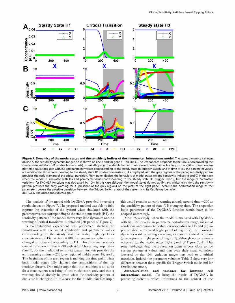
The analysis of the model with DyGloSA provided interesting

results shown on Figure 7. The proposed method was able to fully

capture the dynamics of the system: when simulated with the

parameter values corresponding to the stable homeostasis (H1), the

sensitivity pattern of the model shows very little dynamics and no

warning of critical transitions is obtained (left panel of Figure 7).

A computational experiment was performed: starting the

simulations with the initial conditions and parameter values

corresponding to the steady state of stably high cytokines

concentrations (H3), at time = 180 the parameter values were

changed to those corresponding to H1. This provoked system’s

critical transition at time <290 with state Y becoming larger than

state X, but the method of sensitivity pattern analysis provides the

early warning at time <250 (grey region of middle panel, Figure 7).

The beginning of the grey region is marking the time point when

both model states fully changed the compositions of the top

sensitive clusters. One might argue that this condition is too strict

for a small system consisting of two model states only and that a

warning should already be given when the sensitivity pattern of

one state is changing. In this case for the middle panel example

this would result in an early warning already around time <200 as

the sensitivity pattern of state X is changing then. The respective

input parameter of the DyGloSA function would have to be

adapted accordingly.

Most interestingly, when the model is analyzed with DyGloSA

with (i) 10% increase in parameter perturbation range, (ii) initial

conditions and parameter values corresponding to H3 and (iii) no

perturbation introduced (right panel of Figure 7), the sensitivity

dynamics is still providing a warning for system’s critical transition

(grey regions on right panel of Figure 7), although no transition is

observed for the model states (right panel of Figure 7, A). This

result indicates that the bifurcation point is very close to the

current parameter values and that even their small variations

(covered by the 10% variation range) may lead to a critical

transition. Indeed, the parameter values at Table 3 show very low

difference between those specific for Trigger Switch mode and for

Oscillations mode.

Autocorrelation and variance for immune cell

interactions model. To bring the results of DyGloSA in

predicting system’s critical transitions to the context of the

Figure 7. Dynamics of the model states and the sensitivity indices of the immune cell interactions model. The states dynamics is shownon line A; the sensitivity dynamics for gene X is shown on line B and for gene Y – on line C. The left panel corresponds to the simulation providing thesteady-state solutions H1 (stable homeostasis). In middle panel the simulation with introduced perturbation leading to the critical transition areplotted (simulations start with ICs and parameter values corresponding to the steady state H3 (trigger switch) and at time = 180 the parameter valuesare modified to those corresponding to the steady state H1 (stable homeostasis)). As displayed with the grey regions of the panel, sensitivity patternprovides the early warning of the critical transition. Right panel depicts the behaviors of model states (A) and sensitivity indices (B and C) in the casewhen the model is simulated with ICs and parameter values corresponding to the steady state H3 (trigger switch), but the range of parametervariations for DyGloSA functions was decreased by 10%. In this case although the model states do not exhibit any critical transition, the sensitivitypattern provides the early warning for it (presence of the grey regions on the plots of the right panel) because the perturbation range of theparameters covers the possible transition between the Trigger Switch state of the system and its Oscillatory behavior.doi:10.1371/journal.pone.0082973.g007



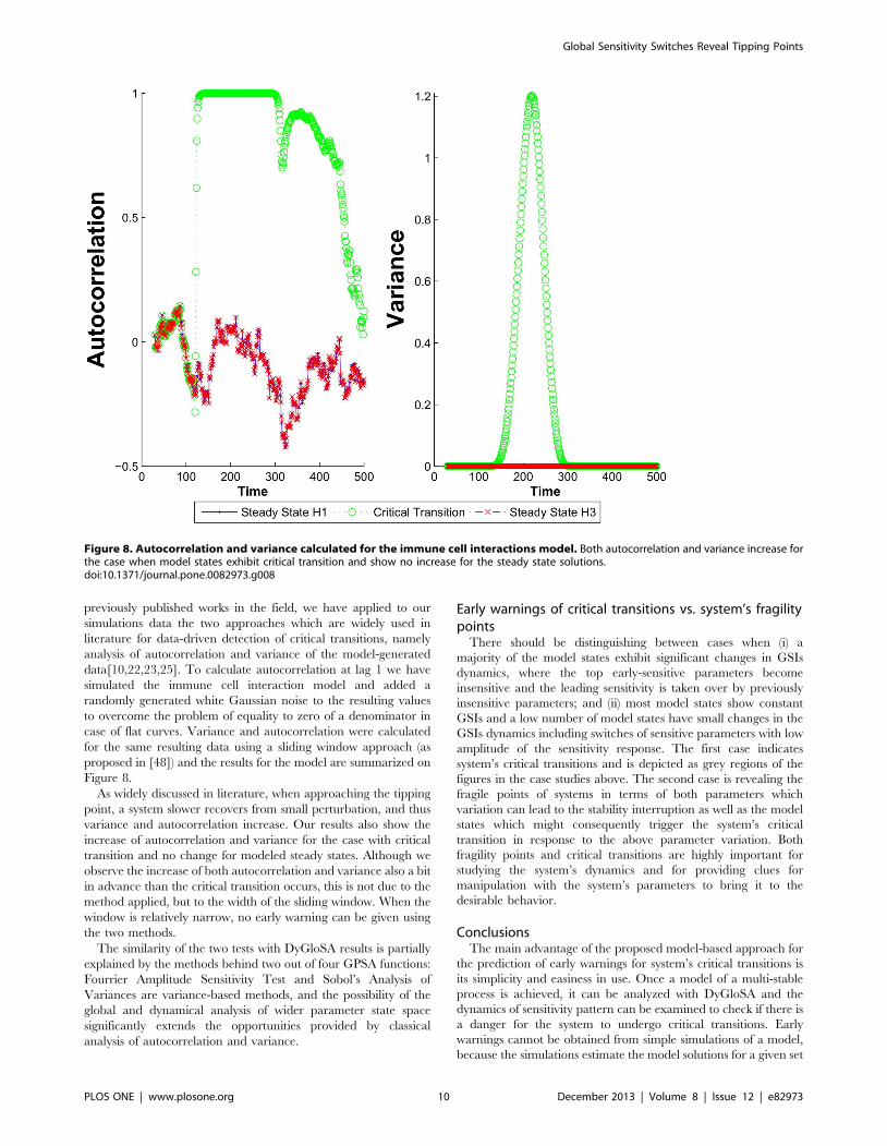
previously published works in the field, we have applied to our

simulations data the two approaches which are widely used in

literature for data-driven detection of critical transitions, namely

analysis of autocorrelation and variance of the model-generated

data[10,22,23,25]. To calculate autocorrelation at lag 1 we have

simulated the immune cell interaction model and added a

randomly generated white Gaussian noise to the resulting values

to overcome the problem of equality to zero of a denominator in

case of flat curves. Variance and autocorrelation were calculated

for the same resulting data using a sliding window approach (as

proposed in [48]) and the results for the model are summarized on

Figure 8.

As widely discussed in literature, when approaching the tipping

point, a system slower recovers from small perturbation, and thus

variance and autocorrelation increase. Our results also show the

increase of autocorrelation and variance for the case with critical

transition and no change for modeled steady states. Although we

observe the increase of both autocorrelation and variance also a bit

in advance than the critical transition occurs, this is not due to the

method applied, but to the width of the sliding window. When the

window is relatively narrow, no early warning can be given using

the two methods.

The similarity of the two tests with DyGloSA results is partially

explained by the methods behind two out of four GPSA functions:

Fourrier Amplitude Sensitivity Test and Sobol’s Analysis of

Variances are variance-based methods, and the possibility of the

global and dynamical analysis of wider parameter state space

significantly extends the opportunities provided by classical

analysis of autocorrelation and variance.

Early warnings of critical transitions vs. system’s fragilitypoints

There should be distinguishing between cases when (i) a

majority of the model states exhibit significant changes in GSIs

dynamics, where the top early-sensitive parameters become

insensitive and the leading sensitivity is taken over by previously

insensitive parameters; and (ii) most model states show constant

GSIs and a low number of model states have small changes in the

GSIs dynamics including switches of sensitive parameters with low

amplitude of the sensitivity response. The first case indicates

system’s critical transitions and is depicted as grey regions of the

figures in the case studies above. The second case is revealing the

fragile points of systems in terms of both parameters which

variation can lead to the stability interruption as well as the model

states which might consequently trigger the system’s critical

transition in response to the above parameter variation. Both

fragility points and critical transitions are highly important for

studying the system’s dynamics and for providing clues for

manipulation with the system’s parameters to bring it to the

desirable behavior.

ConclusionsThe main advantage of the proposed model-based approach for

the prediction of early warnings for system’s critical transitions is

its simplicity and easiness in use. Once a model of a multi-stable

process is achieved, it can be analyzed with DyGloSA and the

dynamics of sensitivity pattern can be examined to check if there is

a danger for the system to undergo critical transitions. Early

warnings cannot be obtained from simple simulations of a model,

because the simulations estimate the model solutions for a given set

Figure 8. Autocorrelation and variance calculated for the immune cell interactions model. Both autocorrelation and variance increase forthe case when model states exhibit critical transition and show no increase for the steady state solutions.doi:10.1371/journal.pone.0082973.g008



of nominal parameter values, either taken from literature, or

obtained experimentally. Based on that, the critical transition can

be revealed with simulations only when the nominal parameter set

has already passed the no-return threshold and the system can’t be

pushed back to its desirable state. In contrast, using dynamical

GPSA, we can predict whether or not a system is in danger of

critical transitions because GPSA methods involve a certain

variation of nominal parameter values. In DyGloSA this variation

is flexible and user-defined, and can be specific to each of the

parameters to ensure that all the relevant biological knowledge is

respected during the analysis.

Availability and Future Directions

DyGloSA is freely available for download at http://bio.uni.lu/

systems_biology/software/dyglosa as a .zip archive which includes

the toolbox functions together with the complete description,

examples and installation guidelines. DyGloSA requires the

installation of MATLAB (versions R2008b or later) and the

Systems Biology Toolbox2 and SBPD available at www.

sbtoolbox2.org. To use the parallelized functions, MATLAB

Parallel Computing Toolbox has to be installed. DyGloSA can be

run on Windows and Linux systems, both -32 and -64 bits.

Since the computation of sensitivity indices is seriously affected

by the PSS sampling method, this fact can define the directions of

DyGloSA development. We plan to implement other sampling

methods, like quasi Monte Carlo sampling, which could improve

the estimation of sensitivity indices for ANOVA and WALS

methods.

Acknowledgments

The authors thank Dr. A. Baumuratov (LCSB, University of Luxembourg)

for the opportunity to perform the simulations on the image processing and

data analysis workstation Intel Xeon E5645 (24 cores, 98 Gb RAM) and

Dr. N. Valeyev (University of Exeter) for the provided comments on the

immune cells interaction model.

Author Contributions

Conceived and designed the experiments: T. Baumuratova TS. Performed

the experiments: T. Baumuratova. Analyzed the data: T. Baumuratova

TS. Contributed reagents/materials/analysis tools: TS T. Bastogne. Wrote

the paper: T. Baumuratova. Developed the software: T. Baumuratova SD.

Read and corrected the manuscript: T. Baumuratova TS T. Bastogne SD.

References

1. Lenton TM, Held H, Kriegler E, Hall JW, Lucht W, et al. (2008) Tipping

elements in the Earth’s climate system. Proceedings of the National Academy ofSciences of the United States of America 105: 1786–1793.

2. Scheffer M, Bascompte J, Brock WA, Brovkin V, Carpenter SR, et al. (2009)

Early-warning signals for critical transitions. Nature 461: 53–59.

3. Scheffer M (2010) Foreseeing tipping points. Nature 467: 411–412.

4. Drake JM, Griffen BD (2010) Early warning signals of extinction in deteriorating

environments. Nature 467: 456–459.

5. Veraart AJ, Faassen EJ, Dakos V, van Nes EH, Lurling M, et al. (2012)

Recovery rates reflect distance to a tipping point in a living system. Nature 481:357–359.

6. Carpenter SR, Cole JJ, Pace ML, Batt R, Brock WA, et al. (2011) Earlywarnings of regime shifts: a whole-ecosystem experiment. Science (New York,

NY) 332: 1079–1082.

7. Hirota M, Holmgren M, Van Nes EH, Scheffer M (2011) Global resilience of

tropical forest and savanna to critical transitions. Science (New York, NY) 334:232–235.

8. Carpenter SR, Brock WA (2011) Early warnings of unknown nonlinear shifts: a

nonparametric approach Reports. Ecology 92: 2196–2201.

9. Lade SJ, Gross T (2012) Early warning signals for critical transitions: a

generalized modeling approach. PLoS computational biology 8: e1002360.

10. Lenton TM, Livina VN, Dakos V, van Nes EH, Scheffer M (2012) Early

warning of climate tipping points from critical slowing down: comparingmethods to improve robustness. Philosophical transactions Series A, Mathemat-

ical, physical, and engineering sciences 370: 1185–1204.

11. Chen L, Liu R, Liu Z-P, Li M, Aihara K (2012) Detecting early-warning signals

for sudden deterioration of complex diseases by dynamical network biomarkers.Scientific Reports 2: 342.

12. Boettiger C, Hastings A (2012) Quantifying limits to detection of early warnings

for critical transitions. Journal of the Royal Society, Interface/the Royal Society.

13. Kambhu J, Weidman S, Krishnan N (2007) New Directions for Understanding

Systemic Risk.

14. May RM, Levin SA, Sugihara G (2008) NEWS & VIEWS Ecology for bankers.

451: 893–895.

15. Brock WA (2004) Tipping Points, Abrupt Opinion Changes, and PunctuatedPolicy Change by.

16. Scheffer M, Carpenter S, Foley JA, Folke C, Walker B (2001) Catastrophic shiftsin ecosystems. Nature 413: 591–596.

17. Venegas J, Winkler T, Musch G (2005) Self-organized patchiness in asthma as a

prelude to catastrophic shifts. Nature 434.

18. Litt B, Esteller R, Echauz J, D’Alessandro M, Shor R, et al. (2001) Epileptic

seizures may begin hours in advance of clinical onset: a report of five patients.Neuron 30: 51–64.

19. McSharry PE, Smith LA, Tarassenko L (2003) Prediction of epileptic seizures:are nonlinear methods relevant? Nature medicine 9: 241–2; author reply 242.

20. Wissel C (1984) A universal law of the characteristic return time near thresholds.

Oecologia 65: 101–107.

21. Held H, Kleinen T (2004) Detection of climate system bifurcations by

degenerate fingerprinting. Geophysical Research Letters 31: 1–4.

22. Dakos V, Scheffer M, van Nes EH, Brovkin V, Petoukhov V, et al. (2008)

Slowing down as an early warning signal for abrupt climate change. Proceedings

of the National Academy of Sciences of the United States of America 105:

14308–14312.

23. Livina VN, Lenton TM (2007) A modified method for detecting incipient

bifurcations in a dynamical system. Geophysical Research Letters 34: 1–5.

24. Kleinen T, Held H, Petschel-Held G (2003) The potential role of spectral

properties in detecting thresholds in the Earth system: application to the

thermohaline circulation. Ocean Dynamics 53: 53–63.

25. Ditlevsen PD, Johnsen SJ (2010) Tipping points: Early warning and wishful

thinking. Geophysical Research Letters 37: 1–10.

26. Biggs R, Carpenter SR, Brock WA (2009) Turning back from the brink:

detecting an impending regime shift in time to avert it. Proceedings of the

National Academy of Sciences of the United States of America 106: 826–831.

27. Schmidt H, Jirstrand M (2006) Systems Biology Toolbox for MATLAB: a

computational platform for research in systems biology. Bioinformatics (Oxford,

England) 22: 514–515.

28. Rodriguez-Fernandez M, Banga JR (2010) SensSB: a software toolbox for the

development and sensitivity analysis of systems biology models. Bioinformatics

(Oxford, England) 26: 1675–1676.

29. Lebedeva G, Sorokin A, Faratian D, Mullen P, Goltsov A, et al. (2012) Model-

based global sensitivity analysis as applied to identification of anti-cancer drug

targets and biomarkers of drug resistance in the ErbB2/3 network. European

journal of pharmaceutical sciences: official journal of the European Federation

for Pharmaceutical Sciences 46: 244–258.

30. Maeda S, Omata M (2008) Inflammation and cancer: role of nuclear factor-

kappaB activation. Cancer science 99: 836–842.

31. Fomekong-Nanfack Y, Postma M, Kaandorp JA (2009) Inferring Drosophila

Gap Gene Regulatory Network: a Parameter Sensitivity and Perturbation

Analysis. BMC Systems Biology 3: 94.

32. Shin SY, Choo SM, Woo SH, Cho KH (2008) Cardiac Systems Biology and

Parameter Sensitivity Analysis: Intracellular Ca 2+ Regulatory Mechanisms in

Mouse Ventricular Myocytes: 25–45. doi:10.1007/10.

33. Zheng Y, Rundell A (2006) Comparative study of parameter sensitivity analyses

of the TCR-activated Erk-MAPK signalling pathway. Systems Biology, IEE

Proceedings, 153(4):201–211, 2006. doi:10.1049/ip-syb.

34. Kontoravdi C, Asprey SP, Pistikopoulos EN, Mantalaris A (2005) Application of

global sensitivity analysis to determine goals for design of experiments: an

example study on antibody-producing cell cultures. Biotechnology progress 21:

1128–1135.

35. Dobre S, Bastogne T, Profeta C, Barberi-heyob M, Richard A (2012) Limits of

variance-based sensitivity analysis for non- identifiability testing in high

dimensional dynamic models. Automatica, 48(11):2740–2749, 2012.

36. Sobol’ IM (2001) Global sensitivity indices for non-linear mathematical models

and their Monte Carlo estimates. Mathematics and Computers in Simulation 55:

271–280.

37. Saltelli A, Ratto M, Andres T, Campolongo F, Cariboni J, et al. (2008) Global

Sensitivity Analysis. The Primer.

38. Saltelli A, Tarantola S, Chan P-S (1999) A Quantitative Model-independent

Method for Global Sensitivity Analysis of Model Output. Technometrics 41: 39–

56.



39. Blower SM, Dowlatabadi H (1994) Sensitivity and Uncertainty Analysis of

Complex Models of Disease Transmission: an HIV Model, as an Example.International Statistical Review 62: 229–243.

40. Bentele M, Lavrik I, Ulrich M, Stosser S, Heermann DW, et al. (2004)

Mathematical modeling reveals threshold mechanism in CD95-inducedapoptosis. The Journal of cell biology 166: 839–851.

41. Huang S, Guo Y-P, May G, Enver T (2007) Bifurcation dynamics in lineage-commitment in bipotent progenitor cells. Developmental biology 305: 695–713.

42. van Voorn G A K, Kooi BW, Boer MP (2010) Ecological consequences of global

bifurcations in some food chain models. Mathematical biosciences 226: 120–133.

43. Letellier C, Aziz-Alaoui MA (2002) Analysis of the dynamics of a realisticecological model. Chaos, Solitons & Fractals 13: 95–107.

44. Eissing T, Conzelmann H, Gilles ED, Allgower F, Bullinger E, et al. (2004)

Bistability analyses of a caspase activation model for receptor-induced apoptosis.The Journal of biological chemistry 279: 36892–36897.

45. Valeyev NV, Hundhausen C, Umezawa Y, Kotov NV, Williams G, et al. (2010)

A systems model for immune cell interactions unravels the mechanism ofinflammation in human skin. PLoS computational biology 6: e1001024.

46. Gardner TS, Cantor CR, Collins JJ (2000) Construction of a genetic toggleswitch in Escherichia coli. Nature 403: 339–342.

47. Savill J, Fadok V (2000) Corpse clearance defines the meaning of cell death.

Nature 407: 784–788.48. Dakos V, Carpenter SR, Brock WA, Ellison AM, Guttal V, et al. (2012) Methods

for detecting early warnings of critical transitions in time series illustrated usingsimulated ecological data. PloS ONE 7: e41010.



Switch of Sensitivity Dynamics Revealed with DyGloSA Toolbox for Dynamical Global Sensitivity Analysis as an Early Warning for System's Critical Transition

Documents