SWEPT FREQUENCY ACOUSTIC TIME DOMAIN REFLECTION MEASUREMENTS OF LGT by SCOTT K. FREDERICK B.A. Physics, Cornell University, 1991 A thesis submitted in partial fulfillment of the requirements for the degree of Master of Science in Electrical Engineering In the department of Electrical and Computer Engineering In the College of Engineering At the University of Central Florida Orlando, Florida Fall Term 1999 Advisor: Donald C. Malocha

Welcome message from author
This document is posted to help you gain knowledge. Please leave a comment to let me know what you think about it! Share it to your friends and learn new things together.
Transcript

SWEPT FREQUENCY ACOUSTIC TIMEDOMAIN REFLECTION
MEASUREMENTS OF LGT
by
SCOTT K. FREDERICKB.A. Physics, Cornell University, 1991
A thesis submitted in partial fulfillment of therequirements for the degree of
Master of Science in Electrical EngineeringIn the department of Electrical and Computer Engineering
In the College of EngineeringAt the University of Central Florida
Orlando, Florida
Fall Term1999
Advisor: Donald C. Malocha

ii
ABSTRACT
An inverse Fourier transform of frequency domain S11 reflection measurements
obtained from precisely cut cube shaped piezoelectric materials produces highly accurate
time domain reflection data with the aid of mathematics and processing. A completely
automated system has been developed to produce time domain reflection measurements
over a temperature range of almost 200°C. The target of the process is the analysis and
extraction of elastic constants of new man made piezoelectric materials such as langasite
(LGS) and langatite (LGT), with the proof of concept based on the analysis of quartz, a
piezoelectric material with well-known physical constants, and the mathematical
simulation of the measurement system.

iii
ACKNOWLEDGMENTS
This research project was partially supported under a contract from the U.S.
Army, Fort Monmouth, NJ, Contract #N66001-97-C-8634. Much thanks to Dr. John Vig
for funding this contract and my research. My advisor, Dr. Don Malocha also earned
much thanks and respect through his work effort and dedication to this project. Mitch
Chou, graduate student, and colleague, helped with data processing and researching
material properties. This project is also indebted to the services of Tom Athos for
acquiring data. Finally, I need to thank my mother and Dr. John Gentile for forking out
the bucks and allowing me to maintain the semi-professional lifestyle that I had become
accustomed to after getting my first degree in 1991.

iv
TABLE OF CONTENTS
LIST OF TABLES . . . . . . . . . . . . . . . . . . . . . . . . . . . . . . . . . . . . . . . . . . . . vi
LIST OF FIGURES . . . . . . . . . . . . . . . . . . . . . . . . . . . . . . . . . . . . . . . . . . . vii
CHAPTER 1 – INTRODUCTION . . . . . . . . . . . . . . . . . . . . . . . . . . . . . . . . . 1
CHAPTER 2 – PHYSICAL AND MATHEMATICAL CONCEPTS . . . . . . . . . . 3
Physical Concepts . . . . . . . . . . . . . . . . . . . . . . . . . . . . . . . . . . . . . . . 3
Mathematical Concepts . . . . . . . . . . . . . . . . . . . . . . . . . . . . . . . . . . . . 4
CHAPTER 3 – EXPERIMENT MEASURING DEVICES . . . . . . . . . . . . . . . . . 7
Transducer . . . . . . . . . . . . . . . . . . . . . . . . . . . . . . . . . . . . . . . . . . . . 7
Transducer Mounting . . . . . . . . . . . . . . . . . . . . . . . . . . . . . . . . . . . . . 7
Measurement Apparatus . . . . . . . . . . . . . . . . . . . . . . . . . . . . . . . . . . . 10
Measurement Tools . . . . . . . . . . . . . . . . . . . . . . . . . . . . . . . . . . . . . . 11
CHAPTER 4 – MATHEMATICAL MODEL . . . . . . . . . . . . . . . . . . . . . . . . . . 14
Acoustical and Electrical Parameters . . . . . . . . . . . . . . . . . . . . . . . . . . . 14
Transducer Only . . . . . . . . . . . . . . . . . . . . . . . . . . . . . . . . . . . . . . . . 16
Transducer / Cube System . . . . . . . . . . . . . . . . . . . . . . . . . . . . . . . . . . 19
Frequency Smoothing . . . . . . . . . . . . . . . . . . . . . . . . . . . . . . . . . . . . . 23
Inverse Fourier Transform . . . . . . . . . . . . . . . . . . . . . . . . . . . . . . . . . . 24

v
CHAPTER 5 – EXPERIMENTAL DATA . . . . . . . . . . . . . . . . . . . . . . . . . . . . 27
Transducer Only . . . . . . . . . . . . . . . . . . . . . . . . . . . . . . . . . . . . . . . . 27
Transducer / Cube . . . . . . . . . . . . . . . . . . . . . . . . . . . . . . . . . . . . . . . 29
CHAPTER 6 - ANALYSIS AND RESULTS . . . . . . . . . . . . . . . . . . . . . . . . . . . 40
Transducer Only . . . . . . . . . . . . . . . . . . . . . . . . . . . . . . . . . . . . . . . . 40
Quartz . . . . . . . . . . . . . . . . . . . . . . . . . . . . . . . . . . . . . . . . . . . . . . . 42
LGT . . . . . . . . . . . . . . . . . . . . . . . . . . . . . . . . . . . . . . . . . . . . . . . . . 47
More Simulation Results . . . . . . . . . . . . . . . . . . . . . . . . . . . . . . . . . . . 52
CHAPTER 7 – CONCLUSION . . . . . . . . . . . . . . . . . . . . . . . . . . . . . . . . . . . 56
APPENDICES . . . . . . . . . . . . . . . . . . . . . . . . . . . . . . . . . . . . . . . . . . . . . . . 58
Appendix A - LabWindows Programs . . . . . . . . . . . . . . . . . . . . . . . . . . 58
Appendix B - Mathcad Simulation of LGT cube with transducer . . . . . . . . 71
REFERENCES . . . . . . . . . . . . . . . . . . . . . . . . . . . . . . . . . . . . . . . . . . . . . . 91

vi
LIST OF TABLES
1. Measurement errors . . . . . . . . . . . . . . . . . . . . . . . . . . . . . . . . . . . . . . 4
2. Zero padding accuracies . . . . . . . . . . . . . . . . . . . . . . . . . . . . . . . . . . . 5
3. Fundamental material properties at room temperature . . . . . . . . . . . . . . . . 22
4. Fundamental material properties at room temperature . . . . . . . . . . . . . . . . 23
5. Zero Padding and first reflected pulse start times . . . . . . . . . . . . . . . . . . . 53

vii
LIST OF FIGURES
1. Picture of transducer mounting compressional device . . . . . . . . . . . . . . . 9
2. Picture of copper housing used to hold cube during measurement process . . 11
3. Picture of complete data taking setup . . . . . . . . . . . . . . . . . . . . . . . . . . 12
4. Electrical representation of piezoelectric material . . . . . . . . . . . . . . . . . . 15
5. Simulated longitudinal transducer S11 response . . . . . . . . . . . . . . . . . . . . 19
6. Simulated S11 response of a longitudinal transducer bonded to a one cm LGTcube . . . . . . . . . . . . . . . . . . . . . . . . . . . . . . . . . . . . . . . . . . . . . . . . . 21
7. Simulated total input impedance of a longitudinal transducer bonded to a onecm LGT cube . . . . . . . . . . . . . . . . . . . . . . . . . . . . . . . . . . . . . . . . . . . 21
8. Simulated S11 response of a longitudinal transducer bonded to a one cm LGTcube with a smoothed curve superimposed (dotted line) . . . . . . . . . . . . . . 24
9. Simulated (transformed) time domain response of a longitudinal transducerbonded to a one cm LGT cube with a smoothed curve superimposed . . . . . 26
10. Measured S11 response of a lithium niobate longitudinal transducer . . . . . . 28
11. Measured S11 response of a lithium niobate shear mode transducer . . . . . . 28
12. Measured S11 response of a lithium niobate longitudinal mode transducerbonded to the X-face of a quartz cube . . . . . . . . . . . . . . . . . . . . . . . . . . 29
13. Measured total Zin of a lithium niobate longitudinal mode transducer bondedto the X-face of a quartz cube . . . . . . . . . . . . . . . . . . . . . . . . . . . . . . . . 30
14. Measured (transformed) time domain response of a lithium niobatelongitudinal mode transducer bonded to the X-face of a quartz cube . . . . . 31

viii
15. Measured (transformed) time domain response of a lithium niobatelongitudinal mode transducer bonded to the X-face of a quartz cube . . . . . 32
16. Measured S11 response of a lithium niobate longitudinal mode transducerbonded to the X-face of an LGT cube . . . . . . . . . . . . . . . . . . . . . . . . . . 33
17. Measured total Zin of a lithium niobate longitudinal mode transducerbonded to the X-face of an LGT cube . . . . . . . . . . . . . . . . . . . . . . . . . . 33
18. Measured (transformed) time domain response of a lithium niobatelongitudinal mode transducer bonded to the X-face of an LGT cube . . . . . . 34
19. Measured (transformed) time domain response of a lithium niobatelongitudinal mode transducer bonded to the X-face of an LGT cube . . . . . . 35
20. Measured S11 response of a lithium niobate shear mode transducerbonded to the X-face of a quartz cube . . . . . . . . . . . . . . . . . . . . . . . . . . 36
21. Measured (transformed) time domain response of a lithium niobate shearmode transducer bonded to the X-face of a quartz cube . . . . . . . . . . . . . . 37
22. Measured S11 response of a lithium niobate shear mode transducer bondedto the X-face of an LGT cube . . . . . . . . . . . . . . . . . . . . . . . . . . . . . . . . 38
23. Measured (transformed) time domain response of a lithium niobate shearmode transducer bonded to the X-face of an LGT cube . . . . . . . . . . . . . . 38
24. Measured (transformed) time domain response of a lithium niobatelongitudinal transducer mounted to the X-face of a quartz cube, detail offirst reflection . . . . . . . . . . . . . . . . . . . . . . . . . . . . . . . . . . . . . . . . . . 43
25. Simulated time domain response of a lithium niobate longitudinal transducermounted to the X-face of a quartz cube, detail of first reflection . . . . . . . . 43
26. Measured (transformed) time domain response of a lithium niobatelongitudinal transducer mounted to the X-face of a quartz cube, detail ofsecond reflection . . . . . . . . . . . . . . . . . . . . . . . . . . . . . . . . . . . . . . . . 44
27. Simulated time domain response of a lithium niobate longitudinal transducermounted to the X-face of a quartz cube, detail of second reflection . . . . . . 44
28. Measured (transformed) time domain response of a lithium niobatelongitudinal transducer mounted to the X-face of a quartz cube, detailof third reflection . . . . . . . . . . . . . . . . . . . . . . . . . . . . . . . . . . . . . . . . 45

ix
29. Simulated time domain response of a lithium niobate longitudinal transducermounted to the X-face of a quartz cube, detail of third reflection . . . . . . . . 45
30. Measured (transformed) time domain response of a lithium niobatelongitudinal transducer mounted to the X-face of an LGT cube, detail offirst reflection . . . . . . . . . . . . . . . . . . . . . . . . . . . . . . . . . . . . . . . . . . 48
31. Simulated time domain response of a lithium niobate longitudinal transducermounted to the X-face of an LGT cube, detail of first reflection . . . . . . . . 48
32. Measured (transformed) time domain response of a lithium niobatelongitudinal transducer mounted to the X-face of an LGT cube, detailof second reflection . . . . . . . . . . . . . . . . . . . . . . . . . . . . . . . . . . . . . . 49
33. Simulated time domain response of a lithium niobate longitudinal transducermounted to the X-face of an LGT cube, detail of second reflection . . . . . . 49
34. Measured (transformed) time domain response of a lithium niobatelongitudinal transducer mounted to the X-face of an LGT cube, detailof third reflection . . . . . . . . . . . . . . . . . . . . . . . . . . . . . . . . . . . . . . . . 50
35. Simulated time domain response of a lithium niobate longitudinal transducermounted to the X-face of an LGT cube, detail of third reflection . . . . . . . . 50

1
CHAPTER 1
INTRODUCTION
Traditionally, velocity measurements in solids have been made using time-based
pulse-echo techniques [1,2,3,4,5]. These techniques used a short, wide-band pulse, or a
gated RF CW signal, to excite a transducer and create an acoustic wave in a solid. The
reflected waves are then measured and recorded in real time. These measurement
methods have limitations due to the required time-base accuracy and have typically been
accomplished by labor intensive manual measurements. Calibration of time delay of the
experimental setup is often difficult and needs great care. Dynamic range and signal to
noise is limited due to the finite input pulse length.
Currently, new technology offers a potentially better method of analyzing time
domain reflection data by acquiring data in the frequency domain and using Fourier
transform and other more advanced signal processing techniques to obtain the time
domain data. Hewlett Packard network analyzers allow for the easy extraction of S-
parameter data using radio frequencies. Measuring S11, the reflected energy in the
frequency domain, of a piezoelectric transducer mounted to a cube of test material allows
for highly accurate acoustical information to be obtained on the material. The network
analyzer allows for calibration to the point of the measurement pins, so the measured data

2
is a representation of the transducer/cube system only, and not additional circuit
parameters introduced by measurement electronics or connection wires.
It will be shown how measured velocities are only limited in accuracy by the
accuracy with which the dimensions of our cubes of test material can be obtained, and by
the interpretations of time domain pulse shapes and phase changes.
This thesis is a proof of the validity of the approach to time domain echo analysis
by using swept frequency measurements and then signal processing to obtain time
domain data. A mathematical model will be used. Experimental data on the well-known
properties of quartz will be presented and compared to industry standard data. Time
domain data from experiment and simulation will be presented and analyzed.
New piezoelectric materials offer increased Q and higher coupling coefficients
over quartz, and are currently a popular research topic with the surface acoustic wave and
bulk acoustic wave communities. The simulation presented is a tool to assist in the
characterization of these new materials.

3
CHAPTER 2
PHYSICAL AND MATHEMATICAL CONCEPTS
Physical Concepts
Complete characterization of a piezoelectric material requires the extraction of the
elastic constants, piezoelectric constants, and the dielectric constants. These constants
are functions of temperature and piezoelectric crystal orientation. Acoustic velocity
measurements over the X, Y, Z, and a 45° axis allow for extraction of 6 elastic constants,
c11, c13, c14, c44, c33, c66, . These constants can then be used to derive the remaining two
elastic constants [6].
Acoustic velocities are necessary to extract elastic constants. The equations
relating elastic constants to the acoustic velocity of a piezoelectric material, are given in
Auld [6]. Acoustic velocities are obtained from the material by measuring the time it
takes for an acoustic wave to traverse a known distance.
It will be shown how measured velocities are only limited in accuracy by the
accuracy with which the dimensions of our cubes of test material can be obtained, and by
the interpretations of time domain pulse shapes and phase changes. This measurement
technique is efficient and accurate over any frequency range of interest, and can be fully
automated using computer control and network analyzers.

4
Reflection time is determined by analyzing pulses in the time domain. Table 1
shows possible inaccuracies due to physical measurements of the 1 cm cubes used in the
experiment, as well as velocity errors that could result from quantization.
Measurement Errors
MeasurementError
Total CubeRound TripDistance
Round TripTime
MeasuredMeasuredVelocity Velocity Error % Error
0 um 2.0000 cm 4.0000 us 5000.0 m/sec 0.0 m/sec 0.000 %
50 um 2.0100 cm 4.0000 us 5025.0 m/sec 25.0 m/sec 0.500 %
10 um 2.0020 cm 4.0000 us 5005.0 m/sec 5.0 m/sec 0.100 %
5 um 2.0010 cm 4.0000 us 5002.5 m/sec 2.5 m/sec 0.050 %
1 um 2.0002 cm 4.0000 us 5000.5 m/sec 0.5 m/sec 0.010 %
2.7 ns 2.0000 cm 4.0027 us 4996.6 m/sec 3.4 m/sec 0.068 %
1.36 ns 2.0000 cm 4.0014 us 4998.3 m/sec 1.7 m/sec 0.034 %
Table 1: Possible inaccuracies in velocity results from physical measurement limitations.
Mathematical Concepts
Frequency data produced by a piezoelectric transducer mounted to a piezoelectric
cube has finite bandwidth. A finite bandwidth implies that there is no frequency
information of interest out of band. This fact allows for the padding of 0dB data points to

5
an S11 frequency data file for the purpose of increasing time domain resolution after a
Fourier transform is executed. Time resolution is limited by Equation 1 when performing
an inverse Fourier Transform.
It is easy to see that resolutions on the order of nanoseconds can be obtained by creating a
signal bandwidth on the order of hundreds of megahertz. Table 2 shows specific
examples of time domain accuracy obtainable in the experiment.
Zero Padding Accuracies
# of Points Bandwidth TimeResolution
1/BW
EquivalentVelocity
Resolution
EquivalentLength
Resolution
% Error
1601 18 MHz 55.5 ns 34 m/sec 277.5 um 0.680 %
2^15 368.63 MHz 2.71 ns 1.7 m/sec 13.6 um 0.034 %
2^16 737.27 MHz 1.36 ns 0.8 m/sec 6.8 um 0.016 %
2^17 1.475 GHz 0.68 ns 0.4 m/sec 3.4 um 0.008 %
2^18 2.95 GHz 0.34 ns 0.2 m/sec 1.7 um 0.004 %
2^19 5.9 GHz 0.17 ns 0.1 m/sec 0.85 um 0.002 %
Table 2: Examples of time domain accuracy obtained by padding zeros in frequency
domain.
bandwidtht
1=∆ )1(

6
For a transducer/cube combination, the S11 frequency data contains information
from the acoustical and electrical properties of the devices. By smoothing the S11
frequency, it is possible to remove the electrical effects of the devices under test and
leave only the acoustic effects. The smoothed curve averages the existing S11 frequency
data and the result is a frequency response that approximates a transducer attached to a
cube of infinite size (no acoustic reflection). Both data files are inverse Fourier
transformed to the time domain, and the smoothed transformed function is then
subtracted from the now transformed S11 data file in time to produce a time domain plot
of the acoustic only frequency response. This resultant time domain data is less noisy
and easier to analyze, as will be shown later.

7
CHAPTER 3
EXPERIMENTAL MEASURING DEVICES
Transducer
The transducers used for this experiment were manufactured by Valpey Fisher.
These transducers were 5 millimeter diameter coax style chrome gold plated Lithium
Niobate overtone polished piezoelectric transducers. The center portion of the transducer
measured 3.3 millimeters.
Both shear and longitudinal mode transducers were used. 36° Y-cut Lithium
Niobate was used for the longitudinal mode data, and 41° X-cut Lithium Niobate was
used for the transverse mode data.
Transducer Mounting
Transducer mounting was a very difficult and important issue in this research
project. Finding a very thin bonding material that would survive a 200°C temperature
range took many weeks of testing, and in the end only partial success was achieved.

8
Photoresist, a readily available liquid used in microelectronics manufacture, was
the first bonding candidate, and ultimately the best. The heat-hardening (curing)
properties of this material, susceptibility to solvents, and the ability to spin the material
down to a sub-micron thickness made it an exceptionally attractive possibility.
Other materials were tried in addition to photoresist. Common Krazy Glue was
tried, but fractured the cube internally during the heating/hardening process, most likely
due to the different thermal expansion properties of the transducer and cube. Good room
temperature results could be obtained with Krazy Glue, if the initial heating/hardening
process was eliminated.
Automotive gasket sealer was also used in several experiments. The gasket sealer
worked well as a couplant, but fell short in two respects. The coupling generally failed
below a minus 30°C, and the consistency of the material was such that it could not be
spun down to sub-micron thickness.
Various other epoxies were tried but did not perform as well as photoresist. Four
different types of photoresist were experimented with. HNR-120 works over the largest
temperature range and was our bonding material of choice. Transducers are easily
removed in a heated bath of xylene after several hours of soaking.
Transducers were mounted by first cleaning both the cube surface and the
transducer with acetone and methanol. A special fixture was made to hold the cube as it
was placed in a spinner. Two drops of photoresist were place on the cube which was then
spun at 6000 rpm for 30 seconds. A mounting plate was then placed on top of the cube.
This plate has a hole just slightly larger than the transducer, and allows for transducer
centering on the cube.

9
After removing the plate, the transducer/cube combination is placed in a spring
loaded compressional device, displayed in Figure 1. Pressure is applied to the transducer
with this apparatus, and the entire device was placed in an oven for 30 minutes or more at
150°C. After the baking process, the transducer mounting is complete.
Figure 1: Picture of transducer mounting compressional device.

10
Measurement Apparatus
A fixture with high thermal conductivity and thermal mass was designed and
manufactured to hold the transducer/cube during measurement over temperature. This
fixture was constructed from a solid copper cylinder. Two piece construction allowed for
the insertion of transducer/cube material into a cube-shaped chamber. Holes were drilled
to hold Omega 25W cartridge heaters. Another hole was drilled to facilitate the addition
of a semi-rigid piece of coax with pogo pins mounted on one end and a female SMA
connector on the other, to make contact with the transducer. A final wire for the T-style
thermocouple was inserted to complete the setup, as shown in Figure 2.
The thermal housing was inserted into a heat tolerant foam, which was then
placed on top of a liquid nitrogen dewar with a small amount of liquid nitrogen in the
bottom. After cooling the housing by direct submersion into liquid nitrogen, the above
setup was then used to gradually heat the housing and transducer/cube over temperature.

11
Figure 2: Picture of copper housing used to hold cube during measurement process.
Measurement Tools
Measurement hardware consisted of a Hewlett Packard 8753B network analyzer,
Yokogawa UP-550-01 temperature controller with T-style thermocouple, and a 400MHz
desktop personal computer with a Windows 95 operating system. Figure 3 shows the
complete data taking setup. The computer used a National Instruments GPIB-AT card to
interface the GPIB bus of the network analyzer. The Yokogawa controller interfaced the
computer via a serial port.

12
Figure 3: Picture of complete data taking setup.
Measurement software consisted of National Instruments LabWindows/CVI
version 5.0, and Yokogawa’s own programming software for the UP series controllers.
National Instruments furnishes a template for controlling the network analyzer on their
website, but this code required substantial modification to take calibrated data across the
bus, take automated measurements over a temperature range, and concurrently monitor
the temperature output of the Yokogawa controller on the serial port of the PC. The code
is included in Appendix A.

13
The Yokogawa controller used its own processing abilities to ramp temperature at
5°C increments with a five minute ramp time and a three minute soak time, starting at
minus 50°C and ending at positive 150°C. The Yokogawa programming software
provides a graphical interface for setting the control parameters and temperature profiles
in the controller. The LabWindows program was only used to monitor temperature
output from the Yokogawa and then take data when the temperature of the
cube/transducer had been stable over several minutes. Stability was determined by
recording temperature history in the LabWindows program. Temperature was measured
every 30 seconds. If each of the last 5 temperature measurements were within 0.5°C of
their average, a data run was taken on the cube/transducer and the temperature was
recorded.

14
CHAPTER 4
MATHEMATICAL MODEL
Acoustical and Electrical Parameters
A transmission line model will be developed to provide a performance simulation.
The Mason model is a commonly used T-style transmission line model that produces
highly accurate simulations [9,10,11,12]. The system modeled here has four parts:
transducer, bond, cube, and parallel load resistor. The transducer is a 3 port device with
one electrical port and two acoustic ports. The bond and cube both have two acoustic
ports, and the load resistor is a single acoustic port device [9,11,12]. The electrical
analogue to our mostly acoustic system is made valid by the assumption that one
electrical ohm equals one acoustical ohm.
This equation is used to calculate the characteristic impedance of the transducer, bond,
and cube in terms of electrical ohms [9,11,12]. Once the characteristic impedance of
each part is known, the impedance is used to create an impedance matrix using a lossy T-
format model as shown in Figure 4. The bond and cube are modeled with a similar
sec11
kgohm = )2(

15
diagram that omits the transformer (no electrical port). Impedance matrices are then
converted into S parameter matrices. S parameter matrices are converted into
transmission matrices, and then cascaded. The resultant single transmission matrix is
converted back to an S parameter matrix and S11 is easily extracted and graphed.
Figure 4: Electrical representation of piezoelectric material.
Input impedance and time domain data are then obtained from the S11 plot.
Appendix B shows a sample simulation for an LGT cube material with a longitudinal
transducer. The details of the appendix will be discussed in the rest of this chapter.

16
Transducer Only
The characteristic impedance of the transducer is obtained by the following
formula in units of kilograms per second [6,11]:
where AT is the transducer surface area, ρT is the density of the transducer material, and vT
is the acoustic velocity of the transducer material. Note that this formula produces only a
real impedance. For a non-ideal case, a loss term is required. The imaginary impedance
term for the transducer is given by [11]:
where ηT is a loss term in units of Newton-seconds per square meter, and f is the
frequency at which the impedance will be measured. For the model, the loss term was
not changed with frequency, and the center frequency of the transducer was used (10
MHz). A loss term on the order of 0.5 generally produces good imaginary impedance
values in the simulation. Some references list this loss term at 0.005 or less [11]. To
obtain the total characteristic impedance of the transducer material, the imaginary and
real terms are simply added together.
Once the characteristic impedance is known, it is used in a 3x3 Z matrix [9,11],
shown in Equation 5, which represents the model shown previously in Figure 4. Note
that force, F, is in units of newtons and can be obtained by multiplying stress by area; it is
TTT vAZ ⋅⋅= ρ0
TTT AfjZ ⋅⋅⋅⋅= ρηπ20
)3(
)4(

17
the acoustic equivalent to volts. Here, area is determined in the plane perpendicular to
the acoustic wave propagation, and represents the active area of the transducer. The
velocity, v, is the acoustic equivalent of current. This matrix is reduced algebraically to a
two port matrix by making the force on the open air end of the transducer equal to zero
[9]. It is very important to make sure the electrical port (V3) becomes port 1 so that later
matrix manipulation will be successful. This requires only algebraic matrix
manipulation.
The other values in the matrix are C0, the static capacitance, and h, a factor that
relates n, the number of turns in the transformer model, to C0. The transformer models
the coupling of the electrical signal into the piezoelectric material. Equations 6 and 7
show how C0 and n are derived [9].
T
Ts
l
AC
⋅=
ε0
0Chn ⋅=
)5(
⋅
⋅⋅
⋅⋅
⋅−=
3
2
1
0
00
00
3
2
1
1
)cot()csc(
)csc()cot(
I
v
v
C
hh
hlZlZ
hlZlZ
j
V
F
F
ωωω
ωββ
ωββ
)6(
)7(

18
In Equation 6, εs is the material permittivity, or dielectric constant in Farads per
meter, AT is the transducer surface area, and lT is height of the piezoelectric disk
transducer, ideally a half wavelength of the resonant frequency. In Equation 7, h is also a
representation for the piezoelectric constant, eT, divided by the dielectric constant, εs.
If the piezoelectric constant is not known, it can also be derived using Equation 8
[11].
This term is given in units of coulombs per meter squared, where k is the dimensionless
coupling coefficient, easily obtained for most commonly used piezoelectric material cuts,
and cT is the transducer stiffness constant. The stiffness constant can be approximated by
known terms as shown in Equation 9, and the units are given in pascals [11].
Using the equations in this section, Appendix B shows how the 2x2 Z matrix is
represented for the transducer model. The appendix also shows how the free air
transducer S11 response is obtained by setting the remaining acoustic port force term
equal to zero. Throughout Appendix B, most impedances are normalized to 50 ohms. A
typical free air transducer response for a simulated longitudinal transducer is shown in
Figure 5.
sTT cke ε⋅⋅= 2
TTT vc ρ⋅= 2 )9(
)8(

19
Figure 5: Simulated longitudinal transducer S11 response prior to mounting on cube.
Transducer / Cube System
Imaginary and real impedances are obtained for the bond and cube as they were
for the transducer, substituting the appropriate terms as they relate to the bond or the cube
material. The material properties of the bond material are not readily known, and the
simulation is used to help predict these properties. The material properties of the cube
are easily measured from our experiment and other physical analysis. It should be noted
that modifying the material properties of the bond in the simulation had little effect in the

20
frequency domain simulation, and even less in the time domain transform. It is assumed
that the density of the bond is low and the velocity is slow with respect to the transducer
and cube materials, yielding a low characteristic impedance. The load resistor, attached
in parallel to the free end of the cube, allows for adjustments to the effective reflection
due to non-idealities such as diffraction scattering and power flow angle effects. In the
ideal case, this resistor would be zero. Small resistance values, with respect to the
normalizing impedance, are used in practice to yield an effective acoustic reflection.
Once all of the 2x2 scattering matrices are obtained from the Z matrices, each
scattering matrix is converted to a transmission matrix. These transmission matrices are
cascaded algebraically into a single transmission matrix which is then converted back to a
scattering matrix that represents the entire system being simulated. Figure 6 shows the
S11 output of the simulation for a longitudinal lithium niobate transducer mounted to a
cube face of LGT perpendicular to the X axis. Figure 7 shows the total input impedance
of the same system, easily obtained from Equation 10.
)10()(1
)(1)(
11
110 fS
fSfZ
−+
=

21
Figure 6: Simulated S11 response of a longitudinal transducer bonded to a one cm LGT
cube.
Figure 7: Simulated total input impedance of a longitudinal transducer bonded to a one
cm LGT cube.

22
The most important material parameters used to generate the simulated figures in
this chapter are shown in Tables 3 and 4. These tables also show material parameters that
can be used to generate simulations of other materials and velocity modes.
Fundamental Material Properties
Material Property Longitudinal ModeLithium Niobate
Transducer
Shear Mode (fast)Lithium Niobate
Transducer
Bond
Velocity 7315.0 m/sec 4525.0 m/sec 2900.0 m/sec
Density 4644.0 kg/m3 4644.0 kg/m3 2400.0 kg/m3
Radius 0.165 cm 0.165 cm 0.160 cm
Loss term 0.9000 N*s/m2 0.9000 N*s/m2 4.000 N*s/m2
Impedance 290 + 4j ohms 180 + 4j ohms 57 + 6j ohms
k 0.33 0.33 N/A
Dielectric Const. 32.0 32.0 N/A
Table 3: Fundamental material properties at room temperature

23
Fundamental Material Properties
Material Property X cut QuartzLongitudinal
X cut Quartz Shear(fast)
X cut LGT Shear(fast)
Velocity 5749.0 m/sec 5103.0 m/sec 3144.0 m/sec
Density 5154.0 kg/m3 5154.0 kg/m3 6150.4 kg/m3
Radius 0.115 cm 0.115 cm 0.115 cm
Loss term 0.4 N*s/m2 0.4 N*s/m2 0.7 N*s/m2
Impedance 93 +1j ohms 83 + 1j ohms 80 + 2j ohms
Table 4: Fundamental material properties at room temperature
Frequency Smoothing
Referring to Figure 6, the large ripples are due to the acoustic echo reflections. If
the cube were infinite in dimension, there would be no ripple (acoustic reflection) and
there would be a smooth S11 profile corresponding to the transducer’s electrical
bandwidth when bonded to the cube. This electrical reflection can be approximated by
smoothing the measured data. This was accomplished by convolving, in the frequency
domain, the measured data with a Hamming window. The resulting smoothed curve is a
good approximation to the S11 that would be obtained with a cube of infinite length (no

24
reflection), leaving only the electrical S11 (see Figure 8). This smoothed curve is then
subtracted from the original raw data to yield the pure acoustic frequency response curve.
Figure 8: Simulated S11 response of a longitudinal transducer bonded to a one cm LGT
cube (solid line) with a smoothed curve superimposed (dotted line).
Inverse Fourier Transform
Figure 9 shows the Inverse Fourier Transform of the previous frequency domain
S11 signal after padding with zeros out to the frequency where 215 frequency points are
obtained. Three methods of padding were tested. Padding with 0dB and 0 phase down in
frequency to near 0 hertz and up in frequency until desired number of points was
obtained, padding with 0dB and 0 phase while smoothing points near the actual measured
data, and padding with the last point measured in the frequency domain when padding to

25
higher frequencies, and padding with the first point measured when padding down to near
0 Hz. In addition, these three methods were experimented with while padding the
measured data only with higher frequencies (no padding between 0 Hz and 1 MHz). All
of these methods are about the same, with variations of pulse start times being a
maximum of 20 nanoseconds, or less than 8 ∆t’s. It is somewhat intuitive to realize that
padding with a slightly non-zero phase term can cause a slight shift in the time domain.
The best results, or most noise-free time domain, are obtained when padding with
the last data point in the data set to the highest frequency of interest and padding with the
first data point down in frequency to near zero hertz. These points are always VERY
close to 0dB, so the term 0 dB padding is still used throughout this paper. This method
was also chosen for analysis here since it was the current method used for data analysis
on most of our existing data. Furthermore, when discussing pulse start times, this paper
is always referring to the smoothed time response, where the electrical effects have been
removed. Again, Table 1, in Chapter 2, shows the resolutions in time that can be
obtained by padding with various numbers of frequency points. Padding is required to
obtain the 0.1% velocity accuracy desired from this project.

26
Figure 9: Simulated (transformed) time domain response of a longitudinal transducer
bonded to a one cm LGT cube (solid line) with a smoothed curve superimposed (dotted
line).
The pulse separations seen in Figure 9 during the later reflections were first
observed in experiment. The first acoustic reflected pulse has a sharp, clean transition
from the noise floor. Subsequent pulses begin to show the internal constructive and
destructive interference produced in the cube-bond-transducer system, indicated by the
multiple zeros within a pulse. The simulation showed that this separation is due to the
cube/transducer interface. Pulses reflect off the cube as well as the back of the
transducer. Note that the electrical response occurs at time of zero and the reflected
pulses occur at regular intervals in time.

27
CHAPTER 5
EXPERIMENTAL DATA
Transducer Only
As mentioned previously, S11 is the parameter measured from the network
analyzer for a transducer or a transducer/cube system under test. Figure 10 shows the S11
data from a longitudinal transducer, and Figure 11 shows the S11 data from a shear
transducer. It was already known that these transducers are not pure or single mode, and
the minor peaks show evidence of the multiple modes. The magnitude of the subordinate
modes is not sufficient to affect the time domain response of the primary mode response
when the transducer is mounted to the cube being tested.

28
Figure 10: Measured S11 response of a lithium niobate longitudinal transducer prior to
mounting to a cube.
Figure 11: Measured S11 response of a lithium niobate shear mode transducer prior to
mounting to a cube.

29
Transducer / Cube
Data of various transducer/cube systems will now be presented. Analysis in the
next chapter will concentrate on longitudinal transducers mounted to LGT and quartz, but
shear mode data is presented here as well for visual reference. All of the data in this
chapter was obtained at room temperature (about 23 degrees C), and a transducer
mounted to the X-face (face perpendicular to the X-axis) was used. All cubes were 1 cm
square within a few microns.
Figure 12: Measured S11 response of a lithium niobate longitudinal mode transducer
(solid line) bonded to the X-face of a quartz cube. The smoothed curve (dotted line) is
obtained using a Hamming function to smooth the measured S11 data.

30
Figure 12 is a representative graph of an S11 frequency data plot of an X-axis
longitudinal data file obtained from a quartz cube. The dotted line in this graph is the
smoothed frequency response. Figure 13 is the total input impedance of the same
cube/transducer system shown in Figure 12 this graph is used as an additional step to
verify results of the simulations.
Figure 13: Measured total Zin of a lithium niobate longitudinal mode transducer bonded
to the X-face of a quartz cube.
Figure 14 shows the IFFT time domain information for the S11 frequency data in
Figure 12. The dotted curve is the plot that results from removing the smoothed data
which approximates the removal of the electrical effects of the cube/transducer
combination. This file was produced by padding zero dB points in the frequency domain
until 215 points were obtained, using the method described in Chapter 4. Figure 15 shows
a close up of the first pulse (first reflection) in the time domain. Again, the dotted curve

31
is the curve without the electrical effects. In this example, there is less than 10
nanoseconds difference in the start time of the smoothed curve and the non-smoothed
(raw data) curve. This represents a velocity difference on the order of 15 meters per
second for our one centimeter cube of quartz.
Figure 14: Measured (transformed) time domain response of a lithium niobate
longitudinal mode transducer bonded to the X-face of a quartz cube (solid line), and the
smoothed curve response (dotted line).

32
Figure 15: Measured (transformed) time domain response of a lithium niobate
longitudinal mode transducer bonded to the X-face of a quartz cube (solid line), and the
smoothed curve response (dotted line).
The velocity obtained from the start point shown in Figure 15 is 5800 meters per
second, which is faster than expected for the room temperature X-cut longitudinal
velocity in quartz of 5750 meters per second, shown in James [1].
Figure 16 is a representative graph of an S11 frequency data plot of an X-axis
longitudinal data file for LGT. The dotted line in this graph is the smoothed frequency
response. Figure 17 is the total input impedance of the cube/transducer system for the
data shown in Figure 16.

33
Figure 16: Measured S11 response of a lithium niobate longitudinal mode transducer
bonded to the X-face of an LGT cube (solid line), and the smoothed curve response
(dotted line).
Figure 17: Measured total Zin of a lithium niobate longitudinal mode transducer bonded
to the X-face of an LGT cube.

34
Figure 18 shows the IFFT time domain information for the S11 frequency data in
Figure 16. Again, the dotted curve in the time domain is the plot that results from
removing the electrical effects. This file was produced by padding zero dB points in the
frequency domain until 215 points were obtained as described in chapter 4. Figure 19
shows a close up of the first pulse (first reflection) in the time domain. Again, the dotted
curve is the curve without the electrical effects. The start time here is chosen when the
smoothed curve has clearly begun to move out of the noise floor. The start time chosen
in Figure 19 corresponds to a velocity of 5602 meters per second.
Figure 18: Measured (transformed) time domain response of a lithium niobate
longitudinal mode transducer bonded to the X-face of an LGT cube (solid line), and the
smoothed curve response (dotted line).

35
Figure 19: Measured (transformed) time domain response of a lithium niobate
longitudinal mode transducer bonded to the X-face of an LGT cube (solid line) with
smoothed response (dotted line).
Figure 20 and Figure 21 show the S11 data and IFFT of a shear mode transducer
quartz cube combination (X-axis), respectively. Again, the dotted plots are the smoothed
functions. Shear mode data usually has a larger dip in the smoothed curve, indicating
stronger electrical coupling into the cube material. Figure 21 shows evidence of multiple
shear modes generated by the shear wave of the transducer. It was difficult to obtain
some slow shear data in cases where fast and slow shear modes were similar in velocity.
The simulation part of the experiment allows for a better approximation of some of the
overlapping modes with its ability to only simulate a single mode response. It was also
shown in the experiment that the orientation of the flat of the shear mode transducer
would allow for the maximizing or minimizing of various shear modes depending on the
mounting angle with respect to the axis of the cube not being measured. When
measuring the X-axis, the orientation is given with respect to the Y and Z axis.

36
Figure 20: Measured S11 response of a lithium niobate shear mode transducer bonded to
the X-face of a quartz cube (solid line), and the smoothed response (dotted line).

37
Figure 21: Measured (transformed) time domain response of a lithium niobate shear
mode transducer bonded to the X-face of a quartz cube (solid line) including smoothed
response (dotted line).
Figure 22 shows the S11 plot of a shear mode transducer bonded to the X-axis face
of an LGT cube. The frequency ripples are closer together here, showing evidence of the
slow shear mode velocity of X-cut LGT. Figure 23 shows the IFFT of the data in Figure
22, and the very slow shear mode velocity, on the order of 2400 meters per second.
Evidence of subordinate longitudinal and fast shear data is noticeable in this figure as
well.

38
Figure 22: Measured S11 response of a lithium niobate shear mode transducer bonded to
the X-face of an LGT cube (solid line) and the smoothed response (dotted line).
Figure 23: Measured (transformed) time domain response of a lithium niobate shear
mode transducer bonded to the X-face of an LGT cube (solid line) and the smoothed
response (dotted line).

39
The amount of data taken during this project was overwhelming. All of it can not
be presented here. Processing and analysis is identical for the other axis of measurement.
It is very possible that the resolution of the time domain data exceeds our ability to pick
proper starting points. When selecting starting points in the time domain of a
transformed frequency domain signal padded with 215 points, it often seems that a point
+/- 2 ∆t’s on either side of the point would be an equally acceptable choice. This could
produce an interpretation error on the order of +/- 3 meters per second of our measured
acoustic velocities. Averaging multiple samples is a possible way to help reduce
interpretation error.

40
CHAPTER 6
ANALYSIS AND RESULTS
This chapter will analyze the similarities and differences of the measured data
with respect to simulated data. Mathematical processing and data interpretation will also
be discussed further.
Transducer Only
The transducer model was the most difficult part of this project, and served as a
benchmark for model correctness, as the S11 plots of free-air transducer are easy to obtain
and use for comparison. One of the difficulties in this comparison is the actual definition
and physical interpretation of a single port S11 measurement. Physically speaking, this is
simply the S11 measurement obtained by attaching two electrodes to a free air transducer.
Mathematically speaking, it is the S11 obtained only after reducing the 3x3 scattering
matrix of the transducer to a single (electrical) port by making the force applied to both
acoustical ports zero. It is not the S11 matrix item from the 2x2 or 3x3 S matrix of the
transducer model. Furthermore, the simulation allowed for a highly
accurate estimation of the loss term required by the transducer. Increasing the loss term
increased the bandwidth of transmitted energy into the transducer.

41
Knowing the other material parameters of our specific cuts of lithium niobate
transducers to good accuracy, the loss term was adjusted to give a waveshape that
matched measured transducer data. This model does not account for subordinate modes
present in the actual transducers, most notably in the shear mode transducer. This feature
will prove to be useful when predicting slow shear modes that can be lost in fast shear
modes of a time domain signal when the velocities are only a few hundred meters per
second different.
Comparing Figures 5 and 10, it can be seen that the modeled transducer S11
response in Figure 5 is similar in magnitude and bandwidth to the actual S11 response
measured in Figure 10. It should be noted that magnitude is closely associated with k
and C0 and can vary by a few dB between different transducers. In simulation and in
experiment, this magnitude difference did not affect the start times of pulses in the time
domain.

42
Quartz
Quartz was chosen as a standard for simulation and for verifying the accuracy of
the experimental data taking process. The physical properties of quartz are easily found
from many publications, although many times this involves extracting properties from
given elastic constants by manipulating formulas found in Auld [6].
Figures 24 and 25, show a close up of the first reflected pulse from an actual
transformed S11 data set taken from the X-axis of a quartz cube mounted with a
longitudinal transducer, and the same simulated data, respectively. This is the same data
set shown in chapter 5. Figures 26 and 27 show the same comparison for the second
reflected pulse, and Figures 28 and 29 show the same time domain close ups for the third
reflected pulse. Again, these time domain plots were obtained from frequency plots
padded with zeros to obtain 215 data points in the frequency domain, and a time resolution
of 2.7 nanoseconds. The markers shown in the figures are the chosen start times, when
the smoothed response curve has clearly left the local noise floor.

43
Figure 24: Measured (transformed) time domain response of a lithium niobate
longitudinal transducer mounted to the X-face of a quartz cube, detail of first reflection
(solid line), and the smoothed response (dotted line).
Figure 25: Simulated time domain response of a lithium niobate longitudinal transducer
mounted to the X-face of a quartz cube, detail of first reflection (solid line), and the
smoothed response (dotted line).

44
Figure 26: Measured (transformed) time domain response of a lithium niobate
longitudinal transducer mounted to the X-face of a quartz cube, detail of second
reflection (solid line), and the smoothed response (dotted line).
Figure 27: Simulated time domain response of a lithium niobate longitudinal transducer
mounted to the X-face of a quartz cube, detail of second reflection (solid line), and the
smoothed response (dotted line).

45
Figure 28: Measured (transformed) time domain response of a lithium niobate
longitudinal transducer mounted to the X-face of a quartz cube, detail of third reflection
(solid line), and the smoothed response (dotted line).
Figure 29: Simulated time domain response of a lithium niobate longitudinal transducer
mounted to the X-face of a quartz cube, detail of third reflection (solid line), and the
smoothed response (dotted line).

46
Analysis of the previous six figures yields a velocity of 5800 m/s for the first
pulse, both measured and simulated; a velocity of 5739 m/s for the measured second
pulse and 5768 m/s for the simulated second pulse; a velocity of 5743 m/s for the
measured third pulse and 5758 for the simulated third pulse. The expected velocity, and
the velocity used in the simulation sheet to develop the physical constants outlined in
chapter 4 is 5750 m/s [1], which is virtually identical to velocities derived from elastic
constants presented in Brice [7] and Salt [8].
A complete analysis of the time domain signal, and the frequency padding method
used to obtain it would be necessary to explain what appears to be a 1% deviation in our
results for the velocity obtained from the first reflected pulse. This analysis is beyond the
scope of this research, and does not seem to be explainable from the basic equations of
the Fourier transforms. Fortunately, this analysis is not required to produce highly
accurate velocities of piezoelectric materials under test if our deviation is consistent.

47
LGT
The same comparison shown for quartz will now be shown for LGT. Figures 30
and 31, show a close up of the first reflected pulse from an actual transformed S11 data set
taken from the X-axis of a quartz cube mounted with a longitudinal transducer, and the
same simulated data, respectively. This is the same data set used in chapter 5. Figures
32 and 33 show the same comparison for the second reflected pulse, and Figures 34 and
35 show the same time domain close ups for the third reflected pulse.

48
Figure 30: Measured (transformed) time domain response of a lithium niobate
longitudinal transducer mounted to the X-face of an LGT cube, detail of first reflection
(solid line), and the smoothed response (dotted line).
Figure 31: Simulated time domain response of a lithium niobate longitudinal transducer
mounted to the X-face of an LGT cube, detail of first reflection (solid line), and the
smoothed response (dotted line).

49
Figure 32: Measured (transformed) time domain response of a lithium niobate
longitudinal transducer mounted to the X-face of an LGT cube, detail of second reflection
(solid line), and the smoothed response (dotted line).
Figure 33: Simulated time domain response of a lithium niobate longitudinal transducer
mounted to the X-face of an LGT cube, detail of second reflection (solid line), and the
smoothed response (dotted line).
50
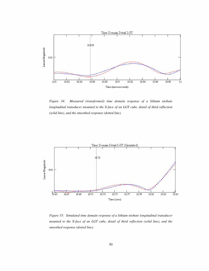
Figure 34: Measured (transformed) time domain response of a lithium niobate
longitudinal transducer mounted to the X-face of an LGT cube, detail of third reflection
(solid line), and the smoothed response (dotted line).
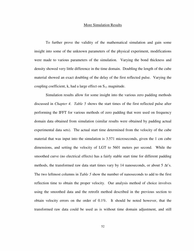
Figure 35: Simulated time domain response of a lithium niobate longitudinal transducer
mounted to the X-face of an LGT cube, detail of third reflection (solid line), and the
smoothed response (dotted line).

51
Analysis of the previous six figures yields a velocity of 5602 m/s for the first
measured pulse, and 5647 m/s for the simulated first pulse; a velocity of 5579 m/s for the
measured second pulse and 5618 m/s for the simulated second pulse; a velocity of 5526
m/s for the measured third pulse and 5597 for the simulated third pulse. The expected
velocity, and the velocity used in the simulation sheet to develop the physical constants
outlined in chapter 4 is 5601 m/s, obtained from our measured (transformed) data on
LGT.
The results are as expected from the information we learned from the quartz
simulation. The data produced by the simulation produces fast velocities with respect to
the velocity used to determine physical constants of the material. If the expected velocity
is reduced to 5558 m/s in the simulation, simulated and measured data become the same
for the first two pulses, and very similar for the third reflected pulse. It could therefore
be assumed that the room temperature longitudinal bulk wave velocity for X-cut LGT is
5558 m/s, which agrees favorably to the 5565 m/s presented in Pisarevsky [13]. This
type of backward analysis and simulation needs to be performed just once for each axis
and mode to find the number of meters per second to subtract from the measured velocity
in question as it is computed from the first reflected pulse.
52
More Simulation Results
To further prove the validity of the mathematical simulation and gain some
insight into some of the unknown parameters of the physical experiment, modifications
were made to various parameters of the simulation. Varying the bond thickness and
density showed very little difference in the time domain. Doubling the length of the cube
material showed an exact doubling of the delay of the first reflected pulse. Varying the
coupling coefficient, k, had a large effect on S11 magnitude.
Simulation results allow for some insight into the various zero padding methods
discussed in Chapter 4. Table 5 shows the start times of the first reflected pulse after
performing the IFFT for various methods of zero padding that were used on frequency
domain data obtained from simulation (similar results were obtained by padding actual
experimental data sets). The actual start time determined from the velocity of the cube
material that was input into the simulation is 3.571 microseconds, given the 1 cm cube
dimensions, and setting the velocity of LGT to 5601 meters per second. While the
smoothed curve (no electrical effects) has a fairly stable start time for different padding
methods, the transformed raw data start times vary by 14 nanoseconds, or about 5 ∆t’s.
The two leftmost columns in Table 5 show the number of nanoseconds to add to the first
reflection time to obtain the proper velocity. Our analysis method of choice involves
using the smoothed data and the retrofit method described in the previous section to
obtain velocity errors on the order of 0.1%. It should be noted however, that the
transformed raw data could be used as is without time domain adjustment, and still

53
produce errors of less than 0.6%. This table is not absolute, and varies by material and
propagation mode.
Table 5: Zero padding and first reflected pulse start times.
First Reflected Pulse Start Times
Padding method
Last frequency point up to desired bandwidth
3.542 usec 3.562 usec 29.0 nsec 9.0 nsec
Zero dB and zero phase up to desired bandwidth
3.542 usec 3.551 usec 29.0 nsec 20.0 nsec
First frequency point down to near zero hertz and last frequency point up to desired bandwidth
3.542 usec 3.548 usec 29.0 nsec 23.0 nsec
Zero dB and zero phase down to near zero hertz
and up to desired bandwidth
3.539 usec 3.551 usec 32.0 nsec 20.0 nsec
down to near zero hertz and up to desired
bandwidth3.542 usec 3.561 usec 29.0 nsec 10.0 nsec
Zero dB and zero phase up to desired bandwidth with gradual transition to
zero dB
3.539 usec 3.551 usec 32.0 nsec 20.0 nsec
Zero dB and zero phase down to near zero hertz
and up to desired bandwidth with gradual transitions to zero dB
3.539 usec 3.551 usec 32.0 nsec 20.0 nsec
Smoothed IFFT Time Response
Curve
Raw Data IFFT Time Response
Curve
Adjustment Required for
Smoothed Curve
Adjustment Required for
Raw Data Curve

54
In addition to simply choosing a start time from the first reflected pulse, it is
possible to subtract the time of the first reflected pulse from the time of the second
reflected pulse to obtain a round trip travel time in the cube. This can be done for
subsequent pulses as well. It is very important to realize that the start of a subsequent
pulse is not necessarily the start of the pulse with the highest magnitude in a “cluster.” It
is generally the start of one of the smaller magnitude pulses that precedes the pulse with
the highest magnitude. Velocities calculated in this manner were within measurement
error of velocities calculated just using the first reflected pulse with respect to zero time.
Time between pulse peaks was also measured, but this method would be expected
to produce skewed results, as it has now been shown that the major peaks of a pulse
involve reflections off the back of the transducer (introduces a time delay). Somewhat of
an improvement over this method is to use the derivative of the time domain to obtain a
peak at a point of maximum slope. This method produces good results for a single
temperature measurement, but is somewhat difficult to automate over temperature. The
analysis program must be given a window in which to look for a peak in the derivative
graph, but the window can be small when dealing with the subordinate pulses that are
close together. As the time domain shifts with temperature, our maximum point can
move outside of the window, making automation over temperature difficult or
impossible.
Although not shown in this report, a set of time domain data over temperature can
be entered into a Matlab program, written primarily by Mitch Chou and Dr. Malocha, to
display a 3-D plot of magnitude vs. time and temperature. These plots show the final
product of this preliminary work, (easily transformed to elastic constants from equations

55
in Auld [6]), and give the experimenter a feeling for how the velocity of the material
under test changes over temperature. It also shows the deterioration of the
transducer/cube bond at high temperatures.

56
CHAPTER 7
CONCLUSION
This research has shown the implementation of a measurement system that was
developed to obtain acoustic velocities of new piezoelectric materials. The validity of
this system was shown using measurements of quartz, a piezoelectric material whose
properties are well known. The validity of the system was also shown using a
mathematical simulation. Basic material properties of the test cubes, transducers, and
bonding material were used as a basis for deriving the impedances used in transmission
line theory, the model used for simulation. A small parallel load resistor was attached to
the end of the cube in the simulation to account for some second and third order effects.
Frequency padding in the time domain was used to increase time domain accuracy
beyond our ability to resolve individual quantization points at the start of a pulse in the
time domain. The results of simulations and measured data sets show the slight time
shifts that can results from padding with even a very small magnitude and phase
component. These shifts in time were consistent and repeatable, and a method of
compensating for time shifts was discussed.
The measurement and simulation process was used on langatite (LGT), a new
piezoelectric material, and results at room temperature of X-axis longitudinal mode
velocity were presented and discussed. Experimental results with quartz verify that the

57
measurement process presented is valid for velocity measurements on any axis of a cubed
material for both shear and longitudinal mode velocities.

58
APPENDIX A
LABWINDOWS CODE

59
The majority of this program was obtained from National Instruments web site. It
is included here to show the additions required to automate the data taking process over
temperature and obtain calibrated data across the bus of the HP network analyzer. The
variable dtype is used to select calibrated data readings from the HP. This change is
made in the user interface (code not shown here). This variable was added to some of
the functions in the code, and the integer for calibrated data was not an option in the
original user interface. Major modifications were made to “configMeasurement,” and
“SaveData,” while “DataRun” and “GetTemp” were created to perform the automation
and temperature retrieval, respectively. Several global variables were also added. Note
that other basic code segments are required to interface the HP network analyzer, and
these segments are included in the basic package downloaded from National Instruments.

60
// modified on 02/22/99 to handle long filenames for datafiles in datarun routine. //
#include <ansi_c.h>#include <utility.h>#include <analysis.h>#include <formatio.h>#include <stdlib.h>#include <userint.h>#include "hp8753x.h"#include "hp8753xu.h"#include "ykut.h" /*for Yokogawa */#include "rs232.h" /*for Yokogawa */
// Before running the UIR you should make sure that the Stack Size is at least 150K// The Stack Size is set in the Project's Options -> Run Options Menu/*= Global Variable Definitions =============================================*/short uirCode;long panelHandle[10];unsigned long instrHandle;double realData[1601], imagData[1601], gFreq[1601];ViStatus uirErr;
int timerstart = 0;double temprecord[2000], templimit;int count, count2, setflag;const char standardstr[20];
/*=================== Utility Function Declarations =========================*/long abortApplication (void);
float GetTemp(void); /*added by skf 11/98 */
/*= Message Arrays ==========================================================*/static char *initCtrlsHelpStr[] = "\nThis control selects the address of the device thatis to be\n" "initialized.\n\n" "Valid Range: Address 0 to 31\n\n" "Default Value: Address 16",
"\nThis control specifies if an ID Query is sent tothe\n" "instrument during the initialization procedure.\n\n" "Valid Range:\n" "VI_OFF (0) - Skip Query\n" "VI_ON (1) - Do Query (Default Value)",
"\nThis control specifies if the instrument is to bereset to its\n" "power-on settings during the initializationprocedure.\n\n" "Valid Range:\n" "VI_OFF (0) - Don't Reset\n" "VI_ON (1) - Reset Device (Default Value)";
static char *configCtrlsHelpStr[] = "This control selects the instrument's examplefunctionality. The\n" "items from the top to the bottom providedinstrument's reset,\n" "configuration of desired parameters and resultmeasurement.\n\n" "Valid Range:\n" "0 - Reset Instrument\n" "1 - Reconfigure Instrument (Default Value)\n" "2 - Measure Only",
"This control selects the desired channel.\n\n" "Valid Range:\n" "VI_OFF (0) - Channel 1 (Default Value)\n" "VI_ON (1) - Channel 2",

61
"This control selects the stimulus mode.\n\n" "Valid Range:\n" "VI_OFF (0) - Continual\n" "VI_ON (1) - Single (Default Value)\n\n" "Notes:\n\n" "(1) Continual:\n" "Select continual sweep.\n\n" "(2) Single:\n" "Execute a single group of sweeps, then hold.",
"This control selects number of measured points forboth channels.\n\n" "Valid Range:\n" "3\n" "11\n" "26\n" "51\n" "101\n" "201 (Default Value)\n" "401\n" "801\n" "1601",
"Desired S-parameter (S11, S21, S12, S22).\n\n" "Valid Range:\n" "0 - S11 (Default Value)\n" "1 - S21\n" "2 - S12\n" "3 - S22",
"This control sets the entry frequency stimulus startvalue.\n\n" "Valid Range: 0.3 to 500000.0\n\n" "Default Value: 100.0 MHz",
"This control sets the entry frequency stimulus stopvalue.\n\n" "Valid Range: 0.3 to 500000.0\n\n" "Default Value: 200.0 MHz",
"I added this control.";
static char backgroundPnlHelpStr[] = "This example presents how to use this instrumentdriver\n" "which supports HP 8753x Network Analyzer.\n\n" "Before running the UIR you should make sure that the\n" "Stack Size is at least 150K!\n" "The Stack Size is set in the Project's Options Menu --> Run Options SubMenu";
static char initPnlHelpStr[] = "This panel performs the following initializationactions:\n\n" "- Opens a session to the Default Resource Managerresource and a\n" "session to the specified device using the interfaceand address\n" "specified in the Resource_Name control.\n\n" "- Performs an identification query on theInstrument.\n\n" "- Resets the instrument to a known state.\n\n" "- Sends initialization commands to the instrumentthat set any\n" "necessary programmatic variables such as Headers Off,Short\n" "Command form, and Data Transfer Binary to the statenecessary\n" "for the operation of the instrument driver.\n\n" "- Returns an Instrument Handle which is used todifferentiate\n" "between different sessions of this instrumentdriver.\n\n" "- Each time this function is invoked a Unique Sessionis opened.\n"

62
"It is possible to have more than one session open forthe same\n" "resource.";
static char configPnlHelpStr[] = "This panel configures the instrument.";
static char measPnlHelpStr[] = "\nThis panel displays the measured values.\n" "Configuration of the instrument is not\n" "possible with this panel. Press the\n" "\"Configure\" button to return to\n" "the configuration panel.";
/*= Main Function ===========================================================*/
void main () // Load panels. panelHandle[BCKGRND] = LoadPanel (panelHandle[BCKGRND], "hp8753xs.uir", BCKGRND); panelHandle[MEAS] = LoadPanel (panelHandle[BCKGRND], "hp8753xs.uir", MEAS); panelHandle[CONFIG] = LoadPanel (panelHandle[BCKGRND], "hp8753xs.uir", CONFIG); panelHandle[INIT] = LoadPanel (panelHandle[BCKGRND], "hp8753xs.uir", INIT); // Display panels. DisplayPanel (panelHandle[BCKGRND]); DisplayPanel (panelHandle[INIT]); SetActiveCtrl (panelHandle[CONFIG], CONFIG_CONTINUE); SetActiveCtrl (panelHandle[MEAS], MEAS_MEASUREMENT);
uirCode = RunUserInterface ();
/*===========================================================================*//* Function: Initialize Instrument *//* Purpose: This is a callback function of the Continue button on the *//* Initialize panel. It initializes the instrument and switches to *//* the panel Configure. *//*===========================================================================*/int CVICALLBACK initInstrument (int panel, int control, int event, void *callbackData, int eventData1, int eventData2)
ViChar instrDescr[256], errorMessage[256], errBuffer[256]; ViInt16 response, addr, rst, id;
switch (event) case EVENT_COMMIT: SetWaitCursor(0); GetCtrlVal (panelHandle[INIT], INIT_ADDRESS, &addr); GetCtrlVal (panelHandle[INIT], INIT_ID, &id); GetCtrlVal (panelHandle[INIT], INIT_RST, &rst); Fmt (instrDescr, "GPIB::%d[b2]", addr); SetWaitCursor(1); if ((uirErr = hp8753x_init (instrDescr, id, rst, &instrHandle)) < 0 ) hp8753x_errorMessage (VI_NULL, uirErr, errorMessage); Fmt (errBuffer, "%s<Initialization Error:\n\n%s\n\nCheck your " "connections and make sure you have the right GPIB address.", errorMessage); MessagePopup ("ERROR!", errBuffer); SetWaitCursor(0); return(0); SetWaitCursor(0); HidePanel (panelHandle[INIT]); DisplayPanel (panelHandle[CONFIG]); break; case EVENT_RIGHT_CLICK: MessagePopup ("Help","This button causes the instrument to be initialized."); break; return 0;
/*===========================================================================*//* Function: Configure Measurement *//* Purpose: This is a callback function of the Continue button on the */

63
/* Configure panel (configure & measure). *//*===========================================================================*/int CVICALLBACK configMeasurement (int panel, int control, int event, void *callbackData, int eventData1, int eventData2) char errMsg[256]; int datatype = 0; int action, channel, stimulus, display, sparam, points =1601; double startFrq, stopFrq;
switch (event) case EVENT_COMMIT: SetWaitCursor(0); HidePanel (panelHandle[CONFIG]); DisplayPanel (panelHandle[MEAS]); GetCtrlVal (panelHandle[CONFIG], CONFIG_SIGTYPE, &datatype); GetCtrlVal (panelHandle[CONFIG], CONFIG_ACTION, &action); GetCtrlVal (panelHandle[CONFIG], CONFIG_CHANNEL, &channel); GetCtrlVal (panelHandle[CONFIG], CONFIG_STIMULUS, &stimulus); GetCtrlVal (panelHandle[CONFIG], CONFIG_SPARAM, &sparam); GetCtrlVal (panelHandle[CONFIG], CONFIG_START, &startFrq); GetCtrlVal (panelHandle[CONFIG], CONFIG_STOP, &stopFrq); SetCtrlVal (panelHandle[MEAS], MEAS_LF, startFrq); SetCtrlVal (panelHandle[MEAS], MEAS_HF, stopFrq); GetCtrlVal (panelHandle[CONFIG], CONFIG_POINTS, &points); DeleteGraphPlot (panelHandle[MEAS], MEAS_GRAPH, -1, VAL_IMMEDIATE_DRAW); SetCtrlAttribute (panelHandle[MEAS], MEAS_GRAPH, ATTR_XAXIS_OFFSET, startFrq); SetCtrlAttribute (panelHandle[MEAS], MEAS_GRAPH, ATTR_XAXIS_GAIN, (stopFrq-startFrq)/points); SetWaitCursor(1);
if ((uirErr = hp8753x_appExample (instrHandle, action, sparam, points,startFrq*1000000.0, stopFrq*1000000.0, channel, realData, imagData, stimulus, datatype)) <0) if (uirErr >= 0xBFFF0000) abortApplication (); else SetWaitCursor(0); hp8753x_errorMessage (VI_NULL, uirErr, errMsg); MessagePopup ("Error", errMsg); return 0; PlotY (panelHandle[MEAS], MEAS_GRAPH, realData, points, VAL_DOUBLE,VAL_THIN_LINE, VAL_NO_POINT, VAL_SOLID, 1, VAL_BLUE); SetWaitCursor(0); break; case EVENT_RIGHT_CLICK: MessagePopup ("Help","This button will configure the instrument to take ameasurement."); break; return 0;
/*===========================================================================*//* Function: Take Measurement *//* Purpose: This is a callback function of the button Measure on the *//* panel Measure. It returns a measurement value without *//* reconfiguring of the instrument. *//*===========================================================================*/int CVICALLBACK takeMeasurement(int panel, int control, int event, void *callbackData, int eventData1, int eventData2) long error, sparam, points = 1601; short dataStatus; int dtype; double primaryValue, secondaryValue; char errMsg[256], rdBuf[256];
switch (event) case EVENT_COMMIT: SetWaitCursor(1);

64
GetCtrlVal (panelHandle[CONFIG], CONFIG_SPARAM, &sparam);GetCtrlVal (panelHandle[CONFIG], CONFIG_SIGTYPE, &dtype);
if ((uirErr = hp8753x_appExample (instrHandle, 2, sparam, points, 1.0e+8, 2.0e+8, VI_OFF, realData, imagData, VI_OFF, dtype)) < 0) if (uirErr >= 0xBFFF0000) abortApplication (); else SetWaitCursor(0); hp8753x_errorMessage (VI_NULL, uirErr, errMsg); MessagePopup ("Error", errMsg); return 0; DeleteGraphPlot (panelHandle[MEAS], MEAS_GRAPH, -1, VAL_IMMEDIATE_DRAW); GetCtrlVal (panelHandle[CONFIG], CONFIG_POINTS, &points); PlotY (panelHandle[MEAS], MEAS_GRAPH, realData, points, VAL_DOUBLE,VAL_THIN_LINE, VAL_NO_POINT, VAL_SOLID, 1, VAL_BLUE); SetWaitCursor(0); break; case EVENT_RIGHT_CLICK: MessagePopup ("Help","This button will return the new meaurement value."); break; return 0;
/*===========================================================================*//* Function: Cancel *//* Purpose: Called by the init panel this function pops up a confirmation *//* dialog box and then quits the user interface, if desired. *//*===========================================================================*/int CVICALLBACK Cancel (int panel, int control, int event, void *callbackData, int eventData1, int eventData2) SetWaitCursor(0); switch (event) case EVENT_COMMIT: if ((ConfirmPopup ("Exit Application", "Are you sure you want to quit this application?")) == 1) QuitUserInterface (uirCode); break; case EVENT_RIGHT_CLICK: MessagePopup ("Control Help", "Closes the application."); break; return 0;
/*===========================================================================*//* Function: Control Help *//* Purpose: This is a callback function of all controls that configure the *//* instrument. On the right mouse-click on the control a help *//* window describing its purpose is displayed. *//*===========================================================================*/int CVICALLBACK controlHelp (int panel, int control, int event, void *callbackData, int eventData1, int eventData2) SetWaitCursor(0); if (event == EVENT_RIGHT_CLICK) if (panel == panelHandle[INIT]) MessagePopup ("Help", initCtrlsHelpStr[control-4]); if (panel == panelHandle[CONFIG]) MessagePopup ("Help", configCtrlsHelpStr[control-2]); return 0;
/*===========================================================================*//* Function: Launch Configure Panel *//* Purpose: This is a callback function of the button Configure on the *//* panel Measure. It returns back to the Configuration panel to be *//* able to change configuration without having to re-run this */

65
/* program. *//*===========================================================================*/int CVICALLBACK launchConfig (int panel, int control, int event, void *callbackData, int eventData1, int eventData2) SetWaitCursor(0); switch (event) case EVENT_COMMIT: HidePanel (panelHandle[MEAS]); DisplayPanel (panelHandle[CONFIG]); break; case EVENT_RIGHT_CLICK: MessagePopup ("Help","This button will recall the configuration panel."); break; return 0;
/*===========================================================================*//* Function: Panel Help *//* Purpose: This is a callback function of the menu bar. It displays a help *//* window describing panel being used. *//*===========================================================================*/void CVICALLBACK panelHelp (int menuBar, int menuItem, void *callbackData, int panel) SetWaitCursor(0); if (panel == panelHandle[BCKGRND]) MessagePopup ("Help", backgroundPnlHelpStr); if (panel == panelHandle[INIT]) MessagePopup ("Help", initPnlHelpStr); if (panel == panelHandle[CONFIG]) MessagePopup ("Help", configPnlHelpStr); if (panel == panelHandle[MEAS]) MessagePopup ("Help", measPnlHelpStr); return;
/*===========================================================================*//* Function: SaveData *//* Purpose: This is a callback function of the button Save on the *//* panel Measure. It pops-up a panel that will prompt for *//* a file name to save data to. *//*===========================================================================*/int CVICALLBACK SaveData (int panel, int control, int event,
void *callbackData, int eventData1, int eventData2)
static double datapoints[1602]; static char pathname[MAX_PATHNAME_LEN], dirname[MAX_PATHNAME_LEN]; int status, num, i, points; double startFrq, stopFrq; static FILE *file_handle;
switch (event)case EVENT_COMMIT:
GetProjectDir (dirname); status = FileSelectPopup (dirname, "datafile.dat", "Datafiles (*.dat)", "DataFile Storage", VAL_SAVE_BUTTON, 0, 1, 1, 1, pathname);
if (status != VAL_NO_FILE_SELECTED) GetCtrlVal (panelHandle[CONFIG], CONFIG_POINTS, &points); GetCtrlVal (panelHandle[CONFIG], CONFIG_START, &startFrq); GetCtrlVal (panelHandle[CONFIG], CONFIG_STOP, &stopFrq); file_handle = fopen (pathname, "w+"); for(i=0; i<points; i++)
gFreq[i] = startFrq + (stopFrq-startFrq)*i/(points-1); num = fprintf (file_handle, "%f, %f, %f\n", gFreq[i], realData[i],imagData[i]);

66
fclose (file_handle);
break;case EVENT_RIGHT_CLICK:
MessagePopup ("Save Button Help", "This button saves the waveform to a data file");
break;
return 0;
/*===========================================================================*//* Function: DataRun *//* Purpose: This is a callback function of the button DataRun on the *//* panel Measure. All temperature values are built in for now. *//* This part of the program automates the data "measure" and"save"*//* buttons on the user interface. Data is aquired and saved
*//* according to an algorithm that keeps track of the last 5measured/* temperatures. The program terminates on a specifictemperature *//* that is entered in the code of the program and a record ofall *//* the measured temperatures is recorded. Temperaturemeasuring *//* intervals are set in the user interface panel (30 seconds),but *//* can be easily changed. Yokogawa temperature controllerruns a *//* temperature ramp on its own. This revision is from 11/98by SKF*//*===========================================================================*/int CVICALLBACK DataRun (int panel, int control, int event,
void *callbackData, int eventData1, int eventData2)
const double deltat = .5; /* reduce as temp profiles arestudied */
const double templimit = 150.0; static double datapoints[1602]; static char pathname[MAX_PATHNAME_LEN], dirname[MAX_PATHNAME_LEN]; const char newfile[100], test1[100]; int status, num, i, points;
double startFrq, stopFrq, degrees, avgtemp; static FILE *file_handle; long error, sparam; short dataStatus; int dtype; double primaryValue, secondaryValue; char errMsg[256], rdBuf[256],tempstr[5], pol[2];
switch (event)case EVENT_COMMIT:
timerstart = 1; /*global variable initially assignedto zero */
ResumeTimerCallbacks();count = 0; /*count keeps track of
the number of times data is recorded and saved */count2 = 0; /*count2 keeps track
of the number of times temperature is measured */setflag = 0;degrees = 19.0;
printf("enter the default string to use in each file name.\n");printf("use the format: XXX_YYY_ZZZ_A_B where X is measurement
type (S11),\n");printf("Y is the material type (QTZ for quartz), \n");printf("Z is the material identifier (012 for example), \n");printf("A is the axis of measurement, and B is the type of wave (L
ongitudinal or S hear).\n");

67
scanf("%s", standardstr);SetStdioWindowVisibility(0);
case EVENT_TIMER_TICK:
setflag = 0;/*measure and display temp */degrees = GetTemp();SetCtrlVal (panelHandle[MEAS], MEAS_CSLIDE, degrees);
/*process degrees here - set flag if degrees is same for last 5temperature readings*/
/* this is the algorithm for taking and saving a datarun. Usetemplimit +1 to guarantee */
/* a data run at templimit */if ( (degrees < (templimit+.5)) && (timerstart != 0) )
temprecord[count2] = degrees;if (count2 >= 4) /* you have atleast 5
temperature measurements */avgtemp = (temprecord[count2]+temprecord[count2-
1]+temprecord[count2-2]+temprecord[count2-
3]+temprecord[count2-4])/5;/*printf("avg %f",avgtemp); */if ((fabs(avgtemp-temprecord[count2])<=deltat) &&
/* last five temperature readings are */ (fabs(avgtemp-temprecord[count2-
1])<=deltat) && /* within deltat of each other then set flag*/ (fabs(avgtemp-temprecord[count2-
2])<=deltat) && (fabs(avgtemp-temprecord[count2-
3])<=deltat) && (fabs(avgtemp-temprecord[count2-
4])<=deltat)) setflag = 1;
count2 = count2+1;if (setflag) /*you want to measure and
save data*/count = count+1;/*measure data and display*/GetCtrlVal (panelHandle[CONFIG], CONFIG_SPARAM,
&sparam);GetCtrlVal (panelHandle[CONFIG], CONFIG_SIGTYPE,
&dtype);GetCtrlVal (panelHandle[CONFIG], CONFIG_POINTS,
&points);SetWaitCursor(1);
if ((uirErr = hp8753x_appExample (instrHandle, 2, sparam, points,/* if there is an error getting data*/
1.0e+8, 2.0e+8, VI_OFF, realData, imagData, VI_OFF, dtype)) < 0) if (uirErr >= 0xBFFF0000) abortApplication (); else SetWaitCursor(0); hp8753x_errorMessage (VI_NULL, uirErr, errMsg); MessagePopup ("Error", errMsg); return 0; /* end if there is an error*/ DeleteGraphPlot (panelHandle[MEAS], MEAS_GRAPH, -1, VAL_IMMEDIATE_DRAW); GetCtrlVal (panelHandle[CONFIG], CONFIG_POINTS, &points); PlotY (panelHandle[MEAS], MEAS_GRAPH, realData, points, VAL_DOUBLE,VAL_THIN_LINE, VAL_NO_POINT, VAL_SOLID, 1, VAL_BLUE); SetWaitCursor(0);

68
/*create file name - pathname from above*/if (count <= 9) Fmt (newfile,
"d:\\dataruns\\%s_%f[p0w3]_00%d.dat", standardstr, degrees ,count);else if ((count > 9)&&(count < 100)) Fmt (newfile,
"d:\\dataruns\\%s_%f[p0w3]_00%d.dat", standardstr, degrees ,count);else Fmt (newfile,
"d:\\dataruns\\%s_%f[p0w3]_00%d.dat", standardstr, degrees ,count);/*save data to file in path above */
GetCtrlVal (panelHandle[CONFIG], CONFIG_START, &startFrq); GetCtrlVal (panelHandle[CONFIG], CONFIG_STOP, &stopFrq); file_handle = fopen (newfile, "w+"); gFreq[0] = startFrq; num = fprintf (file_handle, "%f, %f, %f, %f\n", gFreq[0], realData[0],imagData[0], degrees); for(i=1; i<points; i++)
gFreq[i] = startFrq + (stopFrq-startFrq)*i/(points-1); num = fprintf (file_handle, "%f, %f, %f\n", gFreq[i], realData[i],imagData[i]);
fclose (file_handle); setflag = 0;
/* end if(setflag) */ /* end if less than temp limit */if ( (degrees >= (templimit+.5)) && (timerstart != 0) )
/*save temperature record - you are done*/SuspendTimerCallbacks();timerstart = 0;
Fmt(newfile,"d:\\dataruns\\%stemprec.dat",standardstr);
file_handle = fopen (newfile, "w+"); for(i=0; i<count2; i++) num = fprintf (file_handle, "%f\n", temprecord[i]);
fclose (file_handle);
break; /* EVENT_TIMER_TICK */case EVENT_RIGHT_CLICK:
MessagePopup ("RunData Button Help", "This button runs a program snd temperature dependent algorithm formultiple data runs.");
break; /* end switch (event) */
return 0; /* end CVI callback DataRun */
/*===========================================================================*//* Function: Launch Close Panel *//* Purpose: This is a callback function of the button Close on the *//* panel Measure. It pops-up a panel that will close the *//* instrument. *//*===========================================================================*/int CVICALLBACK launchClose (int panel, int control, int event, void *callbackData, int eventData1, int eventData2) ViChar errorMessage[256], errBuffer[256]; ViInt16 response;
SetWaitCursor(0); switch (event) case EVENT_COMMIT: if ((ConfirmPopup ("Exit Application", "Are you sure you want to quit " "this application?")) == 1) if ((uirErr = hp8753x_close (instrHandle)) < 0) hp8753x_errorMessage(VI_NULL, uirErr, errorMessage); Fmt (errBuffer, "%s<Application failed to close the " "instrument.\n\n%s\n\nExiting Application.", errorMessage); MessagePopup("ERROR!", errBuffer);

69
QuitUserInterface (uirCode); exit (-1); break; case EVENT_RIGHT_CLICK: MessagePopup ("Help","This button will pop-up a panel to close theinstrument."); break; return 0;
/*****************************************************************************/long abortApplication (void) ViChar errorMessage[256], errBuffer[256]; ViInt16 response;
SetWaitCursor (0); hp8753x_errorMessage(VI_NULL, uirErr, errorMessage); Fmt (errBuffer,"%s<The following error caused the application to fail:\n\n%s\n\n" "Attempting to Close Instrument Driver and Exit Application", errorMessage); MessagePopup("ERROR!, Application Failed", errBuffer);
if ((uirErr = hp8753x_close (instrHandle)) < 0) hp8753x_errorMessage(VI_NULL, uirErr, errorMessage); Fmt (errBuffer, "%s<Application failed to close the Instrument Driver.\n\n" "%s\n\nExiting Application.", errorMessage); MessagePopup("ERROR!",errBuffer); else MessagePopup("Application Aborted","Instrument Driver Closed, ExitingApplication.");
QuitUserInterface (uirCode); exit (-1);
return 0;
/*===========================================================================*//* Function: GetTemp *//* Purpose: This is a function used by the callback function of the button *//* DataRun on the panel Measure. It simlpy queries theYokogawa *//* UP550-01 controller for temperature data in degrees celsiuswith*//* two decimal places. Controller must be configured todisplay *//* two decimal places.
*//*===========================================================================*/
float GetTemp(void)
char *hex;const short int STX=0x02, ETX=0x03, CR=0x0D;char *output, *input, *test;int in_len_data = 12, yut_dev_addr = 1,x;static unsigned char yut_out_buffer[256];static char yut_in_buffer[256];unsigned int z;int calc;float mtemp;
Cls(); OpenComConfig(2,"COM2", 9600,2,8,1,256,256); SetCTSMode (2,0); SetXMode(2,0);
/* Fmt (yut_out_buffer, "%c01010INF6%c%c",STX,ETX,CR); IFNEEDED TO VERIFY OPERATION*/ yut_err=0; output=yut_out_buffer;

70
input=yut_in_buffer; FlushOutQ(2); FlushInQ(2);
Fmt (yut_out_buffer, "%c01010WRDD0003,01%c%c", STX, ETX, CR); output=yut_out_buffer; x=ComWrt(2,output, 19);
x=ComRdTerm (2, input, 40, 13); input=yut_in_buffer + 7; /* printf("%s\n",yut_in_buffer); */ Scan (input, "%s>%x4", &calc); /*put 4 bytes of string (hex values) into decimal*/ if (calc > 32768) /* if temp has gone below 0 degreesC */ calc = calc - 65536; mtemp=(calc/100.0); /*change this to 10 if using onedecimal place on controller */ /*printf("The temperature is: %6.2f degrees Celcius.\n", mtemp); */
yut_err=0; yut_close(); return(mtemp); /*return temperature in degrees celsius with 2 decimal places */
/*= End =====================================================================*/

71
APPENDIX B
MATHCAD SIMULATION

72
Transducer - cube matrix model
This file finally has a mathematically correct model for the transducer. Some parameters can still be tweaked a bit, but everything is in the right order of magnitude. The assumption made, and supported by the references is that the acoustic port on the open end of the transducer is a zero in the matrix math, allowing the reduction of the 3x3 matrix to a 2x2. The assumption also made it that one acoustic ohm (kg/s) is equal to one electrical ohm. This version derives the material impedences from the material parameters. Note that the electrical port on the transducer is port 1. This revision furnishes smoothed data and pads frequency points down to near zero. Final version.Padding with first point down to zero and last point up to desired fmax.
Constants:
c 2.99 108. m
s. j 1 dB 1 um 10
6m. f 0 10 MHz. ns 10
9s.
ε 0 8.854 1012. farad
m. uH 10
6H. Z 0 50 ohm. us 10
6s.
Variables:
k .33 Coupling coefficient used for transformer modelling of electrical port on transducer
A k value of .3 will produce an acceptable Zin graph, but k of .4 or so is what is expected.
f start 1 MHz. f stop 19.0000000 MHz. w f( ) 2 π. f.
BW f stop f start ∆fBW
1600f f start f start ∆f, f stop..
∆f =Frequency and material dependent variables:
vlinbL 7315m
sec. vlinbFS 4525
m
sec.
from Mauricio 36 degree Y cut from Mauricio 41 degree X cut
v bond 2900m
sec. estimated by comparing simulation to measured data
material velocities below for LGT Velocities for LGT obtained from our results at room temperature; slow shear velocities are difficult to resolve.
vmxFS 3144m
sec. vmyFS 2844
m
sec. vmzFS 2895
m
sec. vm45FS 3095
m
sec.
vmxSS 3140m
sec. vmySS 2608
m
sec. vm45SS 3090
m
sec.
vmxL 5601m
sec. vmyL 5610
m
sec. vmzL 6587
m
sec. vm45L 6169
m
sec.

73
Set transducer and cube velocities below:
v tran vlinbL v cube vmxL
Use material properties to find impedance of transducer:
radius of active transducer electrode
r tran .00165 m. ρ tran 4644kg
m3
.Mitch - Paper 1994 freq control
use this radius to calculatecapacitance of transducer (physical radius of active portion)
r cap .00172 m.
A tran π r tran2. η tran .9 N.
s
m2
.use .7 increase to get wider BW
Zim01a j w f 0 η tran. ρ tran
. A tran..
Z 01a A tran ρ tran. v tran
. Zim01a
Z 01 Z 01a ohm. s
kg. Z 01a 290.552 4.383i
kg
s=
Use material properties to find impedance of bond:
radius of active transducer electrode
r bond .00160 m. ρ bond 2400kg
m3
. η bond 4 N.s
m2
.
A bond π r bond2.
Zim02a j w f 0 η bond. ρ bond
. A bond..
Z 02a A bond ρ bond. v bond
. Zim02aA bond 8.042 10
6. m2=
Z 02 Z 02a ohm. s
kg.
Z 02 55.976 6.246i Ω=
Use material properties to find impedance of cube:
effective radius after reflection
r cube .00115 m. ρ cube 6150.4kg
m3
. our measurements of LGT
η cube .41 N.s
m2
. .5 works hereA cube π r cube
2.

74
Zim03a j w f 0 η cube. ρ cube
. A cube..
Z 03a A cube ρ cube. v cube
. Zim03a A cube 4.155 106. m
2=
Z 03a 143.125 1.654ikg
s=
Z 03 Z 03a ohm. s
kg.
Z 04 8 ohm j 0. ohm. load resistor for cube
Wavelength and length variables:
λ 1 f( )v tran
fwavelength of bulk wave in transducer LiNbO 3
λ 1 f 0 0.029 in=
λ 2 f( )v bond
fwavelength of bulk wave in bonding material
λ 3 f( )v cube
fwavelength of bulk wave in cube material - change above for mode of propagation
l 1
λ 1 f 0
2propagation length in transducer-changes for shear or longitudinal
l 1 0.014 in=
l 1 .013 in. force to 13 mils from physical measurement
l 2 .5 um. propagation length in bonding material
l 3 1.0 cm. propagation length in cube
Formulas:
β 1 f( )2 π.
λ 1 f( )β 2 f( )
2 π.
λ 2 f( )β 3 f( )
2 π.
λ 3 f( )

75
Use transducer material properties to derive transformer turns ratio for electrical model:
ε s 32 ε 0. lithium niobate dielectric constant Mitch - paper in 1994 IEEE 32
c esc v tran2 ρ tran
.c esc 2.485 10
11. Pa=
e calc k2
c esc. ε s
. lithium niobate piezoelectric constant
e calc 2.769coul
m2
=
A t π r cap2. active area of transducer
C 0
ε s A t.
l 1static capacitance of transducer
C 0 7.975 1012. F=
he calc
ε s8pF from our measured data
nturns h C 0.
nturns 0.078s A.
m=
Now to get impedances of materials:
n nturns
Z 0T 50m kg.
s2
A.. convert acoustic ohms to electrical ohms
n 0.078s A.
m=
C 0 7.975 1012. farad=
Z 01a 290.552 4.383ikg
s=
Z 0T 50s A.
mohm=

76
Use "t" style (Mason) model for transducer with transformer on bottom of center resistor:
Z A1 f( ) j Z 01. tan
β 1 f( ) l 1.
2. Z B1 f( ) j Z 01
. csc β 1 f( ) l 1..
Z1 11 f( ) j
n( )
w f( ) C 0.
2. 1
Z 01a cot β 1 f( ) l 1..
. j1
w f( ) C 0.
.
z1 11 f( )Z1 11 f( )
Z 0Z1 12 f( ) j
h
w f( ). j
h
w f( ).
csc β 1 f( ) l 1.
cot β 1 f( ) l 1.
. m
s A..
z1 12 f( )Z1 12 f( )
Z 0Z1 21 f( ) Z1 12 f( )
z1 21 f( )Z1 21 f( )
Z 0Z1 22 f( ) j Z 01
. cot β 1 f( ) l 1.. j Z 01
.csc β 1 f( ) l 1
. 2
cot β 1 f( ) l 1.
.
z1 22 f( )Z1 22 f( )
Z 0
Graph and results below show low transducer impedance at center frequency
0 1 .107 2 .1070
2 .104
4 .104 Graph of Normalized z11
Frequency
Lin
ear
Mag
nitu
de
z1 11 f( )
f
Z1 11 9.99 MHz.( ) 0.401 2.024i 103. Ω=
Z1 12 9.99 MHz.( ) 319.096i ohm=
Z1 22 9.99 MHz.( ) 1.395 92.493i Ω=
z1 11 9.99 MHz.( ) 8.011 103. 40.486i=
z1 12 f 0 6.373i=
z1 21 f 0 6.373i=
z1 22 f 0 0.028 1.832i=

77
Calculate the reflection coefficient for transducer only, by making acoustic port2 equal to zero
Z tonly f( ) Z1 11 f( )Z1 21 f( ) Z1 12 f( ).
Z1 22 f( ) f 0 1 107. Hz=
Re Z tonly f 0 16.323 Ω=Z tonly f 0 16.323 913.699i Ω=
z tonly f( )Z tonly f( )
Z 0Z1 11 f 0 0.396 2.022i 10
3. Ω=
Z1 12 f 0 318.63i Ω=
S tonly11 f( )z tonly f( ) 1
1 z tonly f( )Z1 21 f 0 318.63i Ω=
Z1 22 f 0 1.382 91.586i Ω=S 11g f( ) 20 log S tonly11 f( ).
2 4 6 8 10 12 14 16 1812
10
8
6
4
2
0
2S11 of Simulated Unmounted Transducer
Frequency
S11
QIm Z tonly 9.46 MHz.( )
Re Z tonly 9.46 MHz.( )
Q 109.122=

78
Impedance for bond, using t-style model:
Z A2 f( ) j Z 02. tan
β 2 f( ) l 2.
2. Z B2 f( ) j Z 02
. csc β 2 f( ) l 2..
Z2 11 f( ) Z A2 f( ) Z B2 f( ) z2 11 f( )
Z2 11 f( )
Z 0Z2 12 f( ) Z B2 f( )
Z2 21 f( ) Z2 12 f( )z2 12 f( )
Z2 12 f( )
Z 0Z2 22 f( ) Z2 11 f( )
z2 21 f( )Z2 21 f( )
Z 0z2 11 10 MHz.( ) 11.531 103.338i=
z2 22 f( )Z2 22 f( )
Z 0 z2 12 10 MHz.( ) 11.532 103.344i=
Impedance for cube, using t-style model:
Z A3 f( ) j Z 03. tan
β 3 f( ) l 3.
2. Z B3 f( ) j Z 03
. csc β 3 f( ) l 3..
Z3 11 f( ) Z A3 f( ) Z B3 f( )z3 11 f( )
Z3 11 f( )
Z 0Z3 12 f( ) Z B3 f( )
Z3 21 f( ) Z3 12 f( ) z3 12 f( )Z3 12 f( )
Z 0Z3 22 f( ) Z3 11 f( )
z3 21 f( )Z3 21 f( )
Z 0
z3 22 f( )Z3 22 f( )
Z 0

79
change Z matrices to S matrices
∆ 1 f( ) z1 11 f( ) 1 z1 22 f( ) 1. z1 12 f( ) z1 21 f( ).
∆ 2 f( ) z2 11 f( ) 1 z2 22 f( ) 1. z2 12 f( ) z2 21 f( ).
∆ 3 f( ) z3 11 f( ) 1 z3 22 f( ) 1. z3 12 f( ) z3 21 f( ).
∆ 1 10 MHz.( ) 32.444 43.374i=
S1 11 f( )z1 11 f( ) 1 z1 22 f( ) 1. z1 12 f( ) z1 21 f( ).
∆ 1 f( )
S1 12 f( )2 z1 12 f( ).
∆ 1 f( )
S1 21 f( )2 z1 21 f( ).
∆ 1 f( )
S1 22 f( )z1 11 f( ) 1 z1 22 f( ) 1. z1 12 f( ) z1 21 f( ).
∆ 1 f( )
S1 11 2.0 f 0. 0.995 0.099i=
this should be very close to 1
S2 11 f( )z2 11 f( ) 1 z2 22 f( ) 1. z2 12 f( ) z2 21 f( ).
∆ 2 f( )
S2 12 f( )2 z2 12 f( ).
∆ 2 f( )
S2 21 f( )2 z2 21 f( ).
∆ 2 f( )
S2 22 f( )z2 11 f( ) 1 z2 22 f( ) 1. z2 12 f( ) z2 21 f( ).
∆ 2 f( )

80
S3 11 f( )z3 11 f( ) 1 z3 22 f( ) 1. z3 12 f( ) z3 21 f( ).
∆ 3 f( )
S3 12 f( )2 z3 12 f( ).
∆ 3 f( )
S3 21 f( )2 z3 21 f( ).
∆ 3 f( )
S3 22 f( )z3 11 f( ) 1 z3 22 f( ) 1. z3 12 f( ) z3 21 f( ).
∆ 3 f( )
parallel load resistor:
This models a parallel resistor attached to the end of our t-line model.
Z R
Z 04 Z 0.
Z 04 Z 0S4 11 f( )
Z R Z 0
Z R Z 0
S4 12 f( )2 Z R
.
Z 0 Z R
S4 21 f( ) S4 12 f( )
S4 22 f( ) S4 11 f( )
S1 11 10 MHz.( ) 0.969 0.071i=
S1 12 11 MHz( ) 0.193 0.15i=
S1 21 10 MHz( ) 0.188 0.141i=
S1 22 11 MHz( ) 0.265 0.93i=
Now convert to transmission (T) matrix:

81
M1 f( )
1
S1 21 f( )
S1 11 f( )
S1 21 f( )
S1 22 f( )
S1 21 f( )
S1 12 f( )S1 11 f( ) S1 22 f( ).
S1 21 f( )
M1 10 MHz.( )3.403 2.546i
3.116 2.707i
2.943 2.701i
3.23 2.549i=
M2 f( )
1
S2 21 f( )
S2 11 f( )
S2 21 f( )
S2 22 f( )
S2 21 f( )
S2 12 f( )S2 11 f( ) S2 22 f( ).
S2 21 f( )
M2 1 MHz.( )1 1.084i 10
3.
1.21 104. 1.285i 10
4.
1.21 104. 1.285i 10
4.
1 1.084i 103.
=
M3 f( )
1
S3 21 f( )
S3 11 f( )
S3 21 f( )
S3 22 f( )
S3 21 f( )
S3 12 f( )S3 11 f( ) S3 22 f( ).
S3 21 f( )
M4 f( )
1
S4 21 f( )
S4 11 f( )
S4 21 f( )
S4 22 f( )
S4 21 f( )
S4 12 f( )S4 11 f( ) S4 22 f( ).
S4 21 f( )
M cascade f( ) M1 f( ) M2 f( ). M3 f( ). M4 f( ).
M cascade 10 MHz.( )4.099 64.089i
0.209 64.151i
3.306 46.411i
0.489 46.461i=
M cascade 1 MHz.( )0 1,
135.912 1.714i 103.=
T 11 f( ) M cascade f( )0 0,
T 12 f( ) M cascade f( )0 1,
T 21 f( ) M cascade f( )1 0,
T 22 f( ) M cascade f( )1 1,

82
T 11 11 MHz.( ) 0.611 62.249i=
T 12 11 MHz.( ) 0.063 45.096i=
T 21 10 MHz.( ) 0.209 64.151i=
T 22 11 MHz.( ) 1.913 45i=
Now convert from T matrix to S matrix parameters
S 11 f( )T 21 f( )
T 11 f( )S 12 f( ) T 22 f( )
T 21 f( ) T 12 f( ).
T 11 f( )
S 21 f( )1
T 11 f( )S 22 f( )
T 12 f( )
T 11 f( )
S 11 10 MHz.( ) 0.997 0.061i= S 12 10 MHz.( ) 9.939 104. 0.016i=
S 21 10 MHz.( ) 9.939 104. 0.016i= S 22 10 MHz.( ) 0.725 5.252i 10
3.=l 2 0.5 um=
f f start f start ∆f, f stop..
Z 01 290.552 4.383i Ω=C 0 7.975 10
12. F=
Z 02 55.976 6.246i Ω=Z 0 50 Ω=
Z 03 143.125 1.654i Ω=h 9.773 10
9. kg m.
s3
A.=
Z 04 8 Ω=n 0.078
s A.
m=
transformer ratio
Graph of S11 for entire system

83
This graph takes two minutes to generatewith 1600 pts.S11graph f( ) 20 log S 11 f( ).
2 4 6 8 10 12 14 16 184
3
2
1
0
1Simulated S11 LGT Longitudinal X-axis
Frequency (MHz)
dB
Put S11 data into an array format that mathcad will use. Simulates data taken from network analyzer
numpoints 1601
i 0 numpoints 1..
freqi f start i ∆f. freq0 1 106. Hz=
1600 ∆f.( ) 1.8 107. Hz=
cplxsigi S 11 freqi
freali Re cplxsigi fimagi Im cplxsigi
Ampi cplxsigi Phi atanfimagi
freali
fi Ampi exp j Phi..
limit max freq( )
Look at total input impedance:f1001 0.975 0.012i=
Z TiZ 0
1 fi
1 fi
.mmm 1000 1001, 1040..

84
1 4.6 8.2 11.8 15.4 190
2400
4800
7200
9600
1.2.104 Total Input Impedance of System
Frequency (MHz)
Ohm
s
Now pad data with "zeros" so that fpoints are obtained. Pad down to near 0Hz and up to where fpoints are obtained.
fpoints 32768 endsm 70
LBW f start 0 Hz. LptsLBW
∆f ILpts trunc Lpts( )
∆f 1.125 104. Hz=
ILpts 88=
numpoints 1.601 103.=
k 0 1, ILpts 1..nfreqk f start ∆f ILpts k( ).
kk ILpts ILpts 1, numpoints ILpts 1..nfreqkk f start kk ILpts( ) ∆f.
kkk numpoints ILpts numpoints ILpts 1, fpoints 1..
nfreqkkk f stop ∆f kkk numpoints ILpts 1( )( ).
lkk ILpts endsm ILpts endsm 1( ), ILpts 1..
hkk numpoints ILpts numpoints ILpts 1, numpoints ILpts endsm 1( )..

85
Ampv S 11 f stop Phv atanIm S 11 f stop
Re S 11 f stop
kksm ILpts endsm ILpts endsm 1( ), numpoints ILpts endsm 1( )..
Ampu S 11 f start Phu atanIm S 11 f start
Re S 11 f start
cplxsigkk
S 11 nfreqkk
cplxsiglkk
S 11 nfreqILpts
cplxsighkk
S 11 nfreqnumpoints ILpts 1
frealkksm
Re cplxsigkksm
fimagkksm
Im cplxsigkksm
Ampk
Ampu Ampkk
cplxsigkk
Ampkkk
Ampv
Phkkk
PhvPh
kPhu Ph
kkatan
fimagkk
frealkk
fkkk
Ampv exp j Phv.( ).fk
Ampu exp j Phu.( ). fkk
Ampkk
exp j Phkk
..
f32767
0.996 0.093i=
f32767
1=
f0
1 5.707i 10 3.=
n 0 fpoints 1..
Now Smooth the data which, in effect, removes the cube reflections
nsmooth 171
sAmpk
AmpusAmp
kkkAmpv
sPhk
PhusPh
kkkPhv
sfk
Ampu exp j Phu.( ).sf
kkkAmpv exp j Phv.( ).
sResk
20 log Ampu( ).sRes
kkk20 log Ampv( ).

86
sreal medsmooth freal nsmooth,( ) simag medsmooth fimag nsmooth,( )
sAmpkksm srealkksm2
simagkksm2
sPhkksm atansimagkksm
srealkksm
sfkksm sAmpkksm exp j sPhkksm.. sReskksm 20 log sAmpkksm
.
flkk sAmplkk exp j sPhlkk.. fhkk sAmphkk exp j sPhhkk
..
t icfft f( )
Substract the smooth function from the measured response yielding only the acoustic reflections :
Netfkkk NetAmpnumpoints ILpts 1 exp j NetPhnumpoints ILpts 1..NetAmpNetAmp
Netfkkk 1025
Netfk NetAmpILpts exp j NetPhILpts..NetAmpNetAmp
Netfk 1025 difference here is actually set to near zero. NetAmp is not used in this
simulation.
Netrealkksm frealkksm srealkksm Netimagkksm fimagkksm simagkksm
Netrealkksm if Netrealkksm 0 1025, Netrealkksm,
NetAmpkksm Netrealkksm2
Netimagkksm2
NetPhkksm atanNetimagkksm
Netrealkksm
Netfkksm NetAmpkksm exp j NetPhkksm..
NetResn 20 log Netfn.
Smooth frequency response :
st icfft sf( )difreal Re t( ) Re st( ) difimag Im t( ) Im st( )
magdifn difrealn2
difimagn2
Pn atanIm tn
Re tnsPn atan
Im stn
Re stn
difPn Pn sPn divPn
Pn sPn
sPn

87
1 4.6 8.2 11.8 15.4 193
2.2
1.4
0.6
0.2
1S11 of total System with Smoothed Data
Frequency (MHz)
dB
In the graph above, the dotted line is the smoothed data, and the solid line is the simulateS11 data.
These are the values used after S11 data is padded with "zeros."
max nfreq( ) 3.686 108. Hz= min nfreq( ) 1 10
4. Hz=

88
Re-calculate the sampling rate dt. dt = (max(freq) - min(freq)) / # of total points-1
BW max nfreq( ) min nfreq( )( ) dfBW
fpoints 1dt
1
BWtn tn
BW 3.686 108. Hz=
Calculate the time range for determining the exact travel time.
timen n( ) dt. tmax fpoints 1( ) dt. tmax 8.889 105. s=
dt 2.713 ns= df 1.125 104. Hz=
0 2.88 5.76 8.64 11.52 14.4 17.28 20.16 23.04 25.92 28.80
0.02
0.04
0.06
Time domain X-cut LGT Simulated
Time (usec)
Lin
ear
Mag
nitu
de
3.45 3.47 3.49 3.51 3.53 3.55 3.57 3.59 3.61 3.63 3.650
0.01
Time Domain Detail LGT (Simulated)
Time (usec)
Lin
ear
Mag
nitu
de
3.5713.545
tt1 3.545

89
7.1 7.12 7.14 7.16 7.18 7.2 7.22 7.24 7.26 7.28 7.30
0.01
Time Domain Detail LGT (Simulated)
Time (usec)
Lin
ear
Mag
nitu
de7.124
tt2 7.124
10.65 10.67 10.69 10.71 10.73 10.75 10.77 10.79 10.81 10.83 10.850
0.01
Time Domain Detail LGT (Simulated)
Time (usec)
Lin
ear
Mag
nitu
de
10.722
tt3 10.722

90
velocity2 cm.
3.571 us. l 2 5 10 7. m=velocity 5.601 103. m
s=
Reflection times using input velocity: Measured reflection times and resultant velocities:
velocity2 cm.
3.571 us. vactual2 cm.
tt1 us.velocity 5.601 103. m
s=
vactual 5.642 103. m
s=
velocity4 cm.
7.142 us.vactual
4 cm.
tt2 us.velocity 5.601 103. m
s=
vactual 5.615 103. m
s=
velocity6 cm.
10.713 us.vactual
6 cm.
tt3 us.velocity 5.601 103. m
s=
vactual 5.596 103. m
s=

91
REFERENCES
[1] B. J. James, Thesis, “Determination of the Elastic and Dielectric Properties of
Quartz,” Royal Holloway and Bedford New College, London Univ., Spring 1987.
[2] B.J. James, “A New Measurement of the Basic Elastic and Dielectric Constants of
Quartz,” 42nd Annual Frequency Control Symposium, pp. 146-154.
[3] G. L. Petersen, B. Chick, W. Junker, “Error Correction Methods in Gated
Amplifier Absolute Velocity Measurements and Comparison with the Pulse-
Echo-Overlap Technique,” IEEE Ultrasonics Symp. Proc. 1975.
[4] W. Soluch, “Measurements of Elastic and Piezoelectric Constants of Li2B4O7
Crystal,” 11th European Frequency and Time Forum, Neuchatel, Mar. 1997, pp.
382-385.
[5] M.A. Breazeale, J.H. Cantrell Jr., J.S. Heyman, “Ultrasonic Wave Velocity and
Attenuation Measurements,” Methods of Experimental Physics, vol. 19, Academic
Press, Inc., 1981, pp. 67-135.

92
[6] B. A. Auld, Acoustic Fields and Waves in Solids,” Second edition. Malbar, FL:
Robert E. Krieger Publishing Company, 1990.
[7] J. C. Brice, “Crystals for Quartz Resonators,” Reviews of Modern Physics, vol.
57, no. 1, pp.105-146, Jan. 1985.
[8] D. Salt, Hy-Q Handbook of Quartz Crystal Devices. Berkshire, England: Van
Nostrand Reinhold Co. Ltd., 1987.
[9] S. Datta, Surface Acoustic Wave Devices. Englewood Cliffs, NJ: Prentice-Hall,
1986.
[10] G. Gonzalez, Microwave Transistor Amplifiers Analysis and Design, Second
Edition. Upper Saddle River, NJ: Prentice Hall, 1997.
[11] V. M. Ristic, Principles of Acoustic Devices. New York, NY: John Wiley and
Sons, Inc., 1983.
[12] A. Ballato, “Bulk and Surface Acoustic Wave Excitation and Network
Representation,” Proc. of the 28th Annual Frequency Control Symp., 1974, pp.
270-279.

93
[13] Y. V. Pisarevsky, P.A. Senyushenkow, B.V. Mill, N. A. Moiseeva, “Elastic,
Piezoelectric, Dielectric Properties of La3Ga5.5Ta0.5O14 Single Crystals,” Proc.
1998 IEEE International Frequency Control Symp., 1998, pp. 742-747.
Related Documents